THE SYMBOLIC TREATMENT OF DIFFERENTIAL GEOMETRY* · 2018-11-16 · THE SYMBOLIC TREATMENT OF DIFFERENTIAL GEOMETRY* BY ARTHUR WHIPPLE SMITH In this paper certain theorems of differential

THE SYMBOLIC TREATMENT OF DIFFERENTIAL GEOMETRY*

BY

ARTHUR WHIPPLE SMITH

In this paper certain theorems of differential geometry have been discussed

and proved by means of a notation similar to that used in the theory of invari-

ants. The notation was first used by Dr. H. Maschke in a paper entitled

A New Method of Determining the Differential Parameters and Invariants

of Quadratic Differential Quantics,\ and later, in a second paper, A Symbolic

Treatment of the Theory of Invariants of Quadratic Differential Quantics

of n Variables. J The use of this notation permits the proving of theorems

without any assumptions as to the character of the parameter lines by which the

surface is represented and has the advantage of showing all invariant expres-

sions in a form which is at once recognizable as invariant. No attempt has been

made to outline general methods for the use of the symbols. Familiarity with the

two papers of Dr. Maschke will be an aid in the acquiring of the small amount

of general method used in this paper.

In this paper the notation is first defined and certain identities are given

which are easily derived from the notations. The symbolic representation of

surface curves and the radius of curvature leads to the derivation of the equa-

tion of the lines of curvature and Euler's formula. Conjugate and asymptotic

lines are defined and their equations obtained. Geodesies are defined from the

symbolic form for geodesic curvature and geodesic torsion is computed by means

of a symbolic form for the direction cosines of the binormal.

The application of the symbols to the determination of a surface from the

coefficients of the first and second fundamental forms is complete with no restric-

tions as to the functions chosen. The cubic form whose vanishing denotes a

contact of the third order with the osculating circle is derived symbolically, as

is also the quadratic form d2r~l¡ds2. The development of this form intro-

duces symbols for magnitudes of order higher than two, and these symbols are

used for obtaining a symbolic equation for the lines of curvature at an umbilic.

A very brief treatment of the characteristic function and its equation serves

* Presented to the Society February 25, 1905. Received for publication January 15, 1905.

fTransactions of the American Mathematical Society, vol. 1 (1900), p. 197.

In the sequel this is referred to as Maschke I.

Jlbid., vol. 4 (1903), p. 415.

33Trans. Am. Math. Soc. 3

License or copyright restrictions may apply to redistribution; see https://www.ams.org/journal-terms-of-use

34 A. w. smith : the SYMBOLIC TREATMENT [January

to show their extreme simplicity of form under the symbolic notation. The

application of symbols to the equations of the rectilinear congruence is shown to

require but a slight modification of the notation already used.

§ 1. Fundamental identities.

This method of treatment depends primarily upon the symbolic representation

of all binary quadratic differential forms as perfect squares. For this purpose

we introduce symbols as follows. Assume

2aa du, duk = (f du2 + f du2 )\

The symbol f has actual meaning only in certain combinations, the simplest

being ffk = aik = aw. The reciprocal of V/a11 a^ — a22 is denoted by ß. The

notation { UV) stands for Ux V2 — U2V^ where the subscripts 1 and 2 repre-

sent differentiation with respect to ux and?«2 respectively. The product ß { UV}

is denoted by ( UV). The following theorem is fundamental : *

If U and V are invariants of a quadratic form, then is also ( UV) invariant.

The following rules are the basis for all symbolic computations :

1) In every symbolic expression of an invariant equivalent symbols may be

interchanged without changing the actual value of the invariant.

2) If the symbolic expression of an invariant is changed only in sign by the

interchange of two equivalent symbols, then the invariant is zero.

The more general of the formulas used are here collected for reference. The

proof of those which are based directly on definitions is omitted. Those for-

mulas which are marked * are true also for the symbol { }. The quantities

a, 6, c, • • ■, £7, V, IF are any functions of ux and u2. The symbols f, </>, ijr,

etc., refer to the form Edu\ + 2Fdux du2 + Gdu\ ; ß is then the reciprocal of

VEG—F2. The symbols F, 4>, ¥, etc., refer to the form

Ddu\ + 2D' duxdu2 + D"du\.

In other words f.fk = 2»^, FiFk= — 2X.¡ct,f a sign 2 here and elsewhere

in this paper denoting summation cyclically with respect to cc, y, z.

(1)» (a6)=-(6a)4

(2)* (a,6c) = 6(ac) + c(a6),

(3)* 6(a6) = J(a62),

(4)* (a6)(cd) -(- (ac)(db) + (ad)(bc) = 0,

* Maschke I, p. 199.

t Bianchi-Lukat, Differentialgeometrie (1899), § 46. In the sequel this reference is given asBianchi.


1906] OF DIFFERENTIAL GEOMETRY 35

(5)* (a,(6c)) + (6,(ca)) + (c,(a6)) = 0,

(6)* ßWÛV^-ßWÛV^ßU^WV^-ßU^WV^ WÜT= UWV;

the last equation defines the symbol WUV;

(7) (a6)A = (aA6) + (a6A) + {a6}^,

(8) W=2,

(9) (f<1>)(fU)(<t>V) = i(f<p)2(UV) = {UV),

(10) (f<p)(f,(<f>W))=0,

(11) {fU)(<?V)l(fU){<pV)-(fV)(<pU)-\ =( UV)2?

the three formulas (9)-(ll) hold also for any set of equivalent symbols, with

the condition that there be also on the left such a factor that a relation similar

to (8) shall exist ;

(12) /«*«(/*) = o, /3/A W = - ßAhif*) -ii

(13) X = (yz), etc., where X, Y, Z are the direction cosines of the normal to

the surface,

(14) *,,= FtFhX- (f<p)(<f>x)fik, etc.,

(15) Xi = (fF){xf)Fi,eUi.,

(16) Fi4>i(F<S>) = 0, ßFl®2(F<S>)=-ßF2l(F<l>)=:%(F<S>)2,

(17)* Z(xU)(xV) = (fU)(fV),

(18) {f^){4>W)\_ßU2(fV)- ßUx{f2V)] = ßW2{UVy) - ßW,(UV2)

-(fcp)(<pW){ u, (fv)) + (ßü){ wvy,

this formula, which also holds for the { } signs if the last term and the factors

ß be omitted, can also be written

-(/4>)(<pW)ÜVf" WÜV-{f<P){<?W){U,{fV))+{ßU){WV},

(19) Z(xW){(xV), U) = -(fW){U,{fV)),

(20)« l.X((xV), U) = (FU)(FV),

(21) (wwk) = - (f<p) \_wwf+(wß){fw }]<j>k,

where wk is defined by duy = ßw2 ds, du2 == — ßwx ds,

(22) {ftp ) ( <p W ) ( F, (fF ) ) = 0, identically in Wk.

•Maschke I, p. 201.


36 A. W. SMITH : THE SYMBOLIC TREATMENT [January

Proofs of formulas.

The following suggestions will aid in the proving of formulas. In general a

parenthesis symbol is to be changed first to the symbol ß { }. This should be

now expanded so as to bring out the coefficients of those factors which have

only the single differentiation, [e. g., formula (19)]. These coefficients will be

of one of two kinds. If they involve no second differentiation of the x, X,

etc., then formulas (1)-(13), (16), (17) are usually sufficient. If such second

differentiations do occur, the use of (7), (14) and (15) will reduce the case to

one of the first kind.

(9) By rule (1),

WifVK + V) = - (fip)(<pU)(fV)

= i(f<p)l(fU)(<t>V)-(fV)(<pU)]

= Hf<f>Y(UV)by(á)

= {UV)by(8).

(13), (14), (15). These results in Christoffel symbols as given by Bianchi *

aredy dz dy ô z

XVEG - F2 = =f =-5T sf , etc.,dWj ou2 ou2 cu1

d2x f 1 2 1 dx Í 1 2 1 Sas _, ^öu-6u-r\ 1 }jH¿+{ 2 k+^'ete"

ôX FD'-GDdx FD - ED' dx-du~[ - EG-F2 dlT, + EG-F2 du~2' etc-

From the definition of the Christoffel symbols follow

These notations lead to formulas (13)—(15) at once.

(18). Commence this proof by expanding (f<f>)(<l>W) ( U, (fV) ) :

Z(xW)((xV),U) = (ßU)-L{xW){xV}

+ ß2U2Z(xW){xV}l-ß2UlZ(xU){xV}i

By (17), ï{xW){xV)={fW){fV}.

By (7), 2.(xW){xV}i=Z(xW){xiV} +2(xW){xVl}.

•Bianchi, ??46-47.t Bianchi, 124.



By (14),

*{xW) {x{V} = Fi { FV} -ZX(xW) - (fcf>) {fV} Z(xW)(<px).

Since "S.Xx. = 0 (from 13), this reduces by the aid of (17) to

-(f<p){1rW)(<p+){fiV},

or, by change of notation, to ( ftp ) ( f W ) ( ̂ ¡r<p ) {yjr{ V } . The term UfV is

replaced by fUV by (6). To the coefficient of (fW) in the whole expression

apply (18), usingyin place of IF and yfr in in place ofy. To this result apply

(9).§ 2. Curves on a surface.

If U(uxu2) = 0 is a curve on the surface given by the equations

x = x(ux, u2), y = y(ux,u2), z = a(«,, u2), then its differential equation is

Uxdux -f U2du2= 0 and along this curve dux/ds and du2/ds may be replaced

by ßp U2 and — ßp Ux respectively, where p is a factor of proportionality. The

direction cosines of the tangent to any curve are dx/ds, dy/ds, dz/ds or, as

they may be written, xxdux/ds + x2du2/ds, etc., and in these new notations the

direction cosines of U= const, will be p(xU),p(yU), p(zU). Since the

sum of the squares of these cosines is unity the value of p is easily found to be

the reciprocal of V(fU)2 = V\U.*

Consider now two curves U= const, and V = const., the factors of propor-

tionality being p and q respectively. Let at be the angle between them. Then

cos <o = pqE(xU)(xV), whence is obtained cos a) = pq ( fU) (fV). From

this follows sin2» = 1 — p2q2(fU)(fV)(<pU)(4>V). Consider now as one

factor p2q2(fU)(<pV) and to the other factor apply formula (4). The result

is sin a>=pq(UV). The angle a> is defined with the condition 0 = £o<7r.

Thus sin co is positive (or 0) and p and q have the same or different signs

according as ( UV) is positive or negative. The differential invariant V(Í7F)

has been found to be (fU)(fV), hence the theorem:

If U and V are to be orthogonal curves, it is necessary and sufficient that

V(t7F) = 0.If U and V are the parameter lines, then this condition reduces to

fxf2 = F = 0. As a further consequence, if V be the integral of the orthog-

onal trajectories of U, then their differential equation is (fU)(fV) = 0 and

from this it follows that F. = m(fU)f and by forming the expression (<pV)2

the factor m is found to be p/q.

* Maschke, I, p. 200 ; Bianchi, ? 23 :

Ail/=/52</£/}*= (/t7)2, V(ÜV)=zßHtV){tV\*=(1U){fV),

ui,U=ßlf,ß{fU}\ = (f, (fU)).



Along any curve IF= const, define wx and w2 by the relations dux = ßw2

and du2 = — ßwx. Then on this curve ds2 = (fw)2. It is desirable to have

a similar expression for the corresponding arc da on the Gaussian sphere. By

definition da2 = 2d"X2 = 'Z(Xw)2. By formulas (15) and (17) this becomes

da2 = ( fF ) ( r/>i> ) ( c/n/r ) ( ff ) ( Fw ) ( ®w ). To this apply formula (9) and let

/', <f>', etc., be symbols of o'er. Thus da2 = (fF)(f&)(Fw)(&w) = (fw)2

and from this identity followsy^ = (fF)F..

Let £7 and F form an isothermal system and also be taken as the parameter

lines, then from the definition of the system must ¿Sx U= A, Fand V ( UV)=0.*

The second of these conditions may be written V. = in(fU)fi and the first is

(f U)2 = (fV)2. This is equivalent to p = ± q and therefore m = ± 1.

Consider now

\y= (/) (fV)) = ±(/> (/*)(*eo)-±(/*) (/. {<pu))±(*U){f (/<*>)).

The first term is zero by formula (10). The second term is seen to be zero

by use of rule (1) and formulas (4), (3), and (8). Thus it is necessary that

A2F= 0. Suppose now that U satisfies A2U=0 and define V by the condi-

tion Fj= (fU)f.. This may be done, for A2U= 0 is the condition that Vt

be an exact differential. Forming A2F from this definition of V{ it follows

as above that A2F= 0. Form now ((pV)^, = (fU)(4>f)<p¡ and consider the

coefficients of Ux and U2 for the cases i = 1, 2. It is seen that Ui=— (fV)f

and from these relations between U and V follow, by rule 2,

V(£TF)- (fU)(fV) = (fU)(f<p)(<t>U) = 0and

^V=(fV)2 = (f<p)(fjr)(<f>U)(yr'U) = (fU)2 = AxU.

The function V¡= (fU)f¡ is called the conjugate solution to U. Hence

the theorem :

In order that U and V form an isothermal system it is a sufficient condi-

tion that A2U= 0 and Vbe the solution conjugate to U.

§ 3. Lines of curvature.

The radius of curvature of curves on a surface may be found as follows.

From the Frenet formulas cos 0/p = ZXd cos a/ds, where p is the radius of

curvature of the curve considered, a, ß, y, are the direction angles of its tan-

gent, and 6 is the angle between the positive direction of the principal normal

and the normal to the surface. Consider in this way the curve <7"= const.

Then cos a=p(xU), etc. Therefore

U^-^/SJ^CT), U)-p(PU)ÏX(xU).

•Bianchi, ? 36.License or copyright restrictions may apply to redistribution; see https://www.ams.org/journal-terms-of-use

1906] OF DIFFEBENTIAL GEOMETRY 39

By (13) the coefficients of Ux and U2 in the expression 1.X(xU) are of the form

2 (yz)Xj which is identically zero. From formula (20), IX((xU), U) = (FUf.

Whence it follows that cos 6/p = p2(FU)2. The curvature of a normal sec-

tion having the same direction as U is found by letting 6 = 0 or tt. If R be

the radius of curvature in that case, and if its sign be so chosen that R is posi-

tive when the center of curvature is on the positive side of the tangential plane,

then 1/R = — p2(FU)2 and p = — R cos 0. This is Meusnier's theorem.*

Lines of curvature are defined as those curves along which the radius of cur-

vature is a maximum or a minimum when considered as dependent on the direc-

tion in which the curve passes through a point. For any one value of 6 con-

sider all the curves which pass through any one point. Then, at this point,

from the relation p = — R cos 6, p is a maximum or a minimum according as

R is a maximum or a minimum. It remains then to find those curves along

which R is a maximum or minimum. The parameter of the normal section is

duxjdu2. Put w = U2J Ux, then (using p for R),

(jvy l/>-/,)2p~ (FU)2~ (Fxw-F2)2'

Therefore

dp _ 2(Flw-F2)2(fxw-f2)fx-2(fxw-f2)2(Fxw-F2)Fxdw (Fxw-F2y

By removing w and simplying the numerator the condition for a maximum or

a minimum becomes (fF)(fU)( FU) = 0 and this is the differential equa-

tion of the lines of curvature. This equation may also be written in the form

U{= h(fF)(FU)f and h may be determined as a function of U by form-

mg (<t>U)2.

Let U be a line of curvature and V be orthogonal to U. Then

U. = n(fV)f{. If this be substituted in the equation for U the equation

(fF)(f<p)(Fyjr)(<pV)(ylrV) = 0 is obtained. This reduces to

(fF)(fV)(FV) = 0,

whence it appears that the lines of curvature form an orthogonal system.

It has been found that X¡ = (fF)(xf)Fr Let now U be a line of curva-

ture so that ( fF)(fU)(FU) = 0. Then

(<pU)2(XU)^(fF)(xf)(FU)(<pU)2.

Apply (4) to (fF)(<f>U) and then (9) to (xf)(<pU)(f<p). These reductions

give (XU) = —p2(FU)2(xU). But since along U the expressions (XU)

and (xU) are proportional to ¿ATand dx respectively, the following theorem is

proved :

•Bianchi, §53.


40 A. W. SMITH : THE SYMBOLIC treatment [January

Along a line of curvature the ratio dx : dX equals the radius of curvature.

§4. Conjugate lines.*

We define as conjugate lines those whose directions satisfy the equation

tan 8X tan 62 = — rx/r2, where 6X and 02 are the angles which the two curves

make with the line of curvature V, and rx and r2 are the values of p along U

and V respectively. Let IF and T be conjugate curves. From the expressions

previously found for sine and cosine a form for the tangent function may be

derived, and from this the differential equation satisfied by IF and Tis

(WV)(TV)_-(fU)2(FV)2

{fT)(fV)(<pW)(4>V)- (fVy(FU)2'

To the expressions (fU)(FV) and (fV)(FU) apply formula (4) and note

that (fU)(fV)= 0. If the equation be now cleared of fractions, the ex-

pression (fF)(fU)(FV)((pW)(<pV)(yfrT)(^V) appears. Apply (4) to

(fU)(<pV),(WV)(FU), and (TV)(fF), remembering that U and Fare

lines of curvature. If now the right member be reduced by means of

(9), the resulting equation of the conjugate lines is (FW)(FT) = 0. From

this it follows that if U and F be conjugate lines, then U( — k(FV)Fi, and if

this value of U. be substituted in (fF)(fU)(FU) = 0, it is seen that F is

a line of curvature. It follows then that the lines of curvature are conjugate.

Also if two curves are conjugate and orthogonal they are lines of curvature-

For, in U{ = k(FV)Fi put Vi=n(fU)f and then form (UU) which is

identically zero. The result is (fF)(fU)(FU) = 0. Thus the conditions

of conjugacy and orthogonality might be taken as the definition of lines of

curvature.

Asymptotic lines are defined as those along which the two conjugate direc-

tions coincide. Their equation is then (FU)2 = 0. -)-

§5. Principal radii. %

The quadratic for the principal radii may be set up as follows:

(FV)2(fU)2 + (FU)2(fV)2Kri-^r2>- (FUf(^V)2

Apply (4) to ( FV)(fU) and to ( FU) (fV), using at the same time the condi-

tions of orthogonality and conjugacy. The numerator becomes then ( UV)2(fF)2.

To the denominator apply (4) and (9). The result is \(UV)2(F®)2. Also

rxr2 — (fUy(<pV)2/(FUy(^> V)2 and by a similar process this is reduced to

2¡(F&)2. The desired quadratic is then

* Bianchi, \\ 54, 56.

+ Bianchi, I 57.

J Bianchi, \ 52.License or copyright restrictions may apply to redistribution; see https://www.ams.org/journal-terms-of-use


(FQyr2 + 2(fF)2r +2 = 0.

Let the total curvature \¡rxr2 be denoted by K and the mean curvature

1/r, + 1/r, by - H, then it follows that 2K= (F<P)2 and H= (fFf, whilethe equation becomes Kr2 + Hr +1 = 0.

Euler's formula. * Let IF= const, be any curve, U, V the lines of curva-

ture, and 8 the angle which IF makes with F(0 = f?<7r). Then

\ = -p2(FU)2 and l = -q2(FV)2.' 1 72

By the condition of orthogonality U may be eliminated from the expression for

rx, the result being

1 (fF)(<pF)(fV)(<pV) .(„v,rmMF,

Also

sin2 8 = a2 ̂? cos2 8 - a2 (lF)(+W)(fVX*V)sin o — q . ,jy y , cos a — q . „^ . 2

Form now in symbols the expression — [cos2#/r2 + sin2 #/r,], reducing it to

a fractional form. In the numerator apply formula (4) to the expressions

(WV)(<pF) and (FV)(fW) and collect the coefficients of (fV)(FW)

and (WV)(FV). By an interchange of t/* and <j>, the first of these becomes

-\_(<t>W)(FV)+( IFF) (<pF)] (fV) (V), which is to be reduced again

by means of (4). The complete term involving (WV)(FV) contains the fac-

tor (fF)(fV)(FV) and is therefore zero. This result in its simplified form

is Euler's formula, viz :

1 cos2 8 sin2 8-=-f--.r r2 rx

In the process of finding the sum — (rx + r2) only the condition of conjugacy

needs to be used. Hence the theorem :

The sum of the radii of curvature of two conjugate normal sections is con-

stant and is — HjK.

If a similar process be applied to the sum of the curvatures of two orthogonal

normal sections, then follows the theorem :

The sum of the curvatures of two orthogonal normal sections is constant

and is — H.

§ 6. Geodesic curvature.|

At any point of a curve C on a surface consider the projection of C on the

tangent plane. The ordinary curvature of this new curve is called the geodesic

* Bianchi, ? 54.

t Bianchi, I 75.



curvature of the curve C. Its computation is as follows. Let U and F be

any two orthogonal curves and let it be required to find the geodesic curvature

of U. Let \jp and 1/p. be the ordinary and the geodesic curvatures respec-

tively. Let 8 be the angle between the principal normal to U and the princi-

pal normal to the curve on the tangent plane. Then 1/p = cos 8¡p.* From

the Frenet formulas we have cos ¡-¡p = d cos a/ds etc., where £, 77, fand a, ß,y

are the direction angles of the principal normal and the tangent respectively.

Along U we have cos a=p(xU), etc., and therefore

COS r*—ff = v{p(xU), U) = p2{(xU), U)+p(pU)(xU).

Since the principal normal to a curve lies in its osculating plane, that of the

projected curve is then the tangent to the curve V. Its direction cosines are

therefore q(xV), etc. Whence it follows that

1-=p2qZ((xU), U)(xV)+pq(pU)Z(xU)(xV).

Since U and F are orthogonal, 1(xU)(xV) = (fU)(fV) = 0 and

Vt= m(fU)f, whence l/pg = p2qm(\U)'L(xx){(xU), U). If in for-mula (19) x is substituted for IF and i/for Fit follows that

2(*X)((*C0, U) = (f<p)(<p1r)(1rX){U,(fU)) = (xf){U,(fU)).

The relation mq = p gives as a final result

l = -p3(f<p)(<pU){U,(fU))."9

The invariant character of this expression is evident from its form.

Geodesic lines are now defined as those curves along which the geodesic cur-

vature is zero. The symbolic form of the equation of the geodesies is then

(f<f>)(<pU){U,(fU))=0.

§ 7. The orthogonal trajectories of geodesics.

Let U be such a curve that its orthogonal trajectories may be given by

V;=p(fU)fr The usual form is Vi = m(fU)f. and since mq=p, it

must be that in this case q = 1, i. e., A, F= 1. The necessary condition that

U. be an exact differential is (/, p(fU)) = 0 or p(f, (fU))+(fp)(fU)=0.Divide the members of this equation by p3, and write the expression p~3(fp)

as — }¡(f, 1/p2)- Replace p~2 by (<f>U)2 and apply (4) to the expression

(<?U)(f, (fU)). The resulting equation is (ftp)(<pU)(U, (fU)) = 0.Hence the theorem :

• Meusnier's theorem, § 3.


1906] OF differential geometry 43

If the orthogonal trajectories of a curve are given by Vi = p(fU)fi then

the curve is a geodesic and AJ F= 1.

If a be the constant of integration in V, then

3A,F d( fV) ( dV\â—H/v)^ = HfV)(f,^) = o.

Therefore V(F, dV/da) = 0 and the curves dV/oa = const, are the orthogo-

nal trajectories of the curves F = const.

From this follows the theorem :

The integral equation of the geodesies in terms of their orthogonal trajec-

tories V is d Vf da = 0.

§ 8. The cosines of the binormal.

The direction cosines of the binormal of a curve are proportional to the dif-

ferences (y'z" — z'y"), etc., where the accents denote differentiation with respect

to s. Along any curve IF let

dux = ßw2ds = ßt W2ds and du2 = — ßwx ds = — ßt Wx ds,

these relations being the definitions of wi and t2 = (fW)2.

Then y = (yw), y" = ((yw), w) and therefore

y'z" — z'y" = (yw) ((zw), w) — (aw) ((yw), w)

= ßw2[(yw)(zxw) — (zw)(yxw)~\ — ßwx [(yw)(z2w) - (zw)(y2w)]

+ ßwi l(yw)(zwi) — (zw)(yî)'\ — ßwi [(y«>)(2M>2) — (zw)(yw2y\.

Apply (4) to the third and fourth terms obtaining ßw2(yz)(wwx). and

— ßwx (yz)( ww2 ) respectively. From the identity ( y w ) ( zi w ) = ß2 {y w} {zi w}

compute the differences (yw)(z¡w) — (zw)(y.w). These contain terms

y.zik — z yik which, by the elimination of zik, yik, become

FiFk[yjZ-z.r]-(f<p)[yJ(^)-zJ(<t>y)-]fik.

If Z and Y be expressed in terms of œ, y, z then

yJZ-z.Y=-(fx)fj. Also yj(<pz) ~ zj(<py) = (yz)<pJ.

From these results follows

*,** - v« = - FiFAf*)f, - (/^)(y)^/«-Consequently

(yw)(ziw) - (zw)(y{w) = - (fx)(fw)(Fw)F. - (f<p)(<pw)(f.w)(yz).


44 a. w. smith : the symbolic treatment [January

If this be substituted in the original equation, the result is

y'z"—z'y"= (yz)[ßw2(wwx)—ßwx(ww2)—( f<p) (<pw) { ßw3( fxw)—ßwx( f2w)}]

-(fx)(fw)(Fw)2.

In formula (18) put U= V= W=w and apply it to the coefficient of (yz). If

t?(f<p)(<pW)(W, (/IF)) be denoted by G and if the notation IF,, be used

instead of w{, the desired proportion takes the form

cos X : cos n : cos v= G (yz) - ? (fx ) (fW) ( F Wf : G(zx) - ?(fy) (fW) (F W )2

:G(xy)-f(fz)(fW)(FWy.

From this are easily derived expressions for the cosines of the principal normal

of a geodesic. For if f, 17, f ba the direction angles, then

cos £ = cos u cos y — cos v cos ß, etc.

Along a geodesic G is zero and therefore

cos \ : cos m : cos v = (fx) (fW) : (fy)(fW) : (fz)(frV).

Also coa a: cos ß : cosy = (xW) : (yW) : (zW) and by substitution in the

above identity it follows that

cos I : cos r) : cos f= (yz) : (ax) : (xy).

But since 2(xy )2 = 1,

cos £ = =h X, cos n = ± Y, cos f = ± Z.

For an asymptotic line (iÎF)2 = 0 and therefore as above

cos A = ± X, cos p. =s ± Y, cos i/ = ±Z,

From these considerations follows the theorem :

The surface normal along a geodesic line coincides with the principal nor-

mal and along an asymptotic line with the binormal.

§9. Geodesic torsion.

The Frenet expression for torsion is 1/ T= — 2 cos Xd cos £/ds.* Let U be

a geodesic line. Then along U, cos £ = ± X, etc., cos A = ^pp(fx)(fU).

The factor of proportionality is found to be p by evaluating the expression

2 [(fjc)(fU)Y. Its sign is — or + according as cos £ is ± X, as is seen

from cos a = cos r¡ cos v — cos feos p.. Also from (15),

^*=±p(XU) = ±V(fF)(xf)(FU).

* Bianchi, § 84.



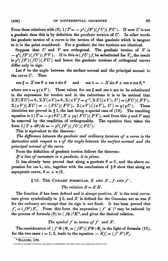
From these relations with (9), \¡T= - p2(fF)(fU)(FU). If now ¿7 is not

a geodesic then this is by definition the geodesic torsion of U. In other words

the geodesic torsion of a curve is the torsion of that geodesic which is tangent

to it in the point considered. For a geodesic the two torsions are identical.

Suppose that U and V are orthogonal. The geodesic torsion of V is

- q2(/F)(fV)(FV). If in this m(fU)f. be substituted for V{, the result

is p2(fF)(fU)(FU) and hence the geodesic torsions of orthogonal curves

differ only in sign.

Let 8 be the angle between the surface normal and the principal normal to

the curve U. Then

cos £ = A" cos 8 + cos a sin 8 and cos X = — A" sin 8 + cos a cos 8, *

where cos a = q(xV). These values for cos £ and cos A are to be substituted

in the expression for torsion and in the reductions it is to be noticed that

•ZX(XU) = 0,-ZX(xV)=0,-Z(xV)2 = q-2,-ZX((xV),U)=(FU)(FV),

•L(xV)(XU)=-(FU)(FV), 2(xF)((xF), U) = q(qU). Theseidentities are proved in § 1, the last being a special case of (19). The resulting

equation is 1/T= — p (8U)X+ pq(FU)(FV), and from this a and F may

be removed by the condition of orthogonality. The equation then takes the

form 1/T+ d8/ds=-p2(fF)(fU)(FU}.This is equivalent to the theorem :

The difference between the geodesic and ordinary torsions of a curve is the

derivative with respect to s of the angle between the surface normal and the

principal normal of the curve.

From the definition of geodesic torsion follows the theorem :

If a line of curvature is a geodesic, it is plane.

It has already been proved that along a geodesic 0 = 0, and the above ex-

pression for cos X, etc., together with the conclusions of § 8 show that along an

asymptotic curve, 8 = + ir/2.

§10. The Codazzi formulas, ß and /3',/and/'.

The relation ß = ß'K.

The function ß has been defined and is always positive, K is the total curva-

ture given symbolically in § 5, and ß' is defined for the Gaussian arc as was ß

for the ordinary arc except that its sign is not fixed. It has been proved that

f\ = (fF)Fi. From this form the expression {f <f>' }2 may be reduced by

the process of formula (9) to {ff> }2K2, and gives the desired relation.

The symbol f in terms of f and F.

The consideration of (/'<$)<!>. = (fF)(F®)<t>.'m the light of formula (16),

for the two cases i = 1, 2, leads to the equation — Kf = (f F) Fr

•Bianchi, §85.License or copyright restrictions may apply to redistribution; see https://www.ams.org/journal-terms-of-use


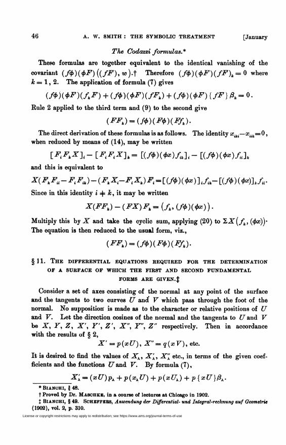
The Codazziformulas*

These formulas are together equivalent to the identical vanishing of the

covariant (f<f>)(<pF) ((fF), w).f Therefore (ßp)(<pF)(fF)k= 0 where

k = 1, 2. The application of formula (7) gives

(f<P)(<pF)(fkF) + (f<P)(<PF)(fFk) + (f<p)(<PF){fF}ßk=0.

Rule 2 applied to the third term and (9) to the second give

(FFk) = (f<p)(F<p)(Ffk).

The direct derivation of these formulas is as follows. The identity xM—xiik= 0,

when reduced by means of (14), may be written

i^F.Xl- IF^X]^ [(«#)(*)/.]<■- [(/*)(**)/„]»

and this is equivalent to

x(jFt^-^<Ji)-(JF;^-^xj^l-[(^)(^)]l/a-[(>»)(*B)],/..

Since in this identity i 4= k, it may be written

X(FFk)-(FX)Fk={fk,(f4>)(<?x)).

Multiply this by X and take the cyclic sum, applying (20) to 2AT(/4, (<px))-

The equation is then reduced to the usual form, viz.,

{FFk) = (f<P)(F<p)(Ffk).

§11. The differential equations required for the determination

of a surface of which the first and second fundamental

forms are given. $

Consider a set of axes consisting of the normal at any point of the surface

and the tangents to two curves U and! V which pass through the foot of the

normal. No supposition is made as to the character or relative positions of U

and F. Let the direction cosines of the normal and the tangents to Í7and F

be A', Y, Z, X', Y', Z', X", Y", Z" respectively. Then in accordance

with the results of § 2,

X' =p(xU), X"=q(xV), etc.

It is desired to find the values of Xk, X'K, X"K etc., in terms of the given coef-

ficients and the functions U and F. By formula (7),

_X'K = (xU)p,+p(xKU) + p(xUK) + p{xU}ßK.

• Bianchi, \ 48.

f Proved by Dr. Maschke, in a course of lectures at Chicago in 1902.

% BIANCHI, § 49. Scheffehs, Anwendung der Differential- und Inlegral-rechnung auf Geometrie

(1902), vol. 2, p. 310.



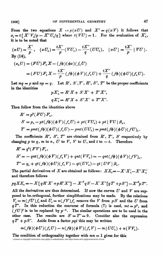
From the two equations X --p(xU) and X" = q(xV) it follows that

xi = t[X' V./p — X"UJq] where t(VU) = 1. For the evaluation of X'k,

it is to be noted that

X' tX' tX" tX'(xU) = ^, (xUk) = --(VUk)---(UUk), {xU}=--{VU}.

By (14),

(xkU) = (FU)FkX- (f<f>)(<px)(AU)

tX' tX"= (FU)FkX---(f<P)(<pV)(fkU) + -q-(f<p)(<t>U)(fkU).

Let mq= p and np = q. Let R', S', T', R", S", T" be the proper coefficients

in the identities

PX'k = RX+ S'X' + TX",

qX"k = R"X+ S"X' + T"X".

Then follow from the identities above

R' =p2(FU)Fk,

S,=p„-pt(f<p)(<?V)(fKU)+pt(VUK)+pt{VU}ßK,

T'=pmt(f<p)(<f>U)(fkU)-pmt(UUk)=pmt(f<p)(<pU)(fU)k.

The coefficients R", S", T" are obtained from R', T', 8' respectively by

changingp to q, m to n, U to V, V to U, and t to — t. Therefore

R"=q2(FV)Fk,

S"=-qnt(f<?)(<pV)(fkV) + qnt(VVK)=-qnt(f<p)(<pV)(fV)K,

T"=qk + qt(f<p)(<pU)(AV)-qt(UVK)-qt{UV}ßk.

The partial derivatives of A" are obtained as follows : XXk=— X'X'k—X"X'K'

and therefore follows

pqXXk =- X[qR'X'+pR"X"] - X'2qS'-X'X"[qT'+pS"] -X"2pT".

All the derivatives are thus determined. If now the curves U and F are sup-

posed to be. orthogonal, further simplifications may be made. By the relations

V. = m(fU)fi and Ui = n(fV)fi remove the F from pS' and the U fromq T". In this reduction the converse of formula (7) is used, mt=p2, and

(fU)2 is to be replaced by p~2. The similar operations are to be used in the

other case. The results are S' = T" = 0. Consider also the expression

qT' -\- pS". Aside from a factor pqt this may be written

m(f^)(<?U)(fhU)-n(f<t>)(<pV)(fKV)-m(UUK) + n(VVk).

The condition of orthogonality together with mn = 1 gives for thisLicense or copyright restrictions may apply to redistribution; see https://www.ams.org/journal-terms-of-use


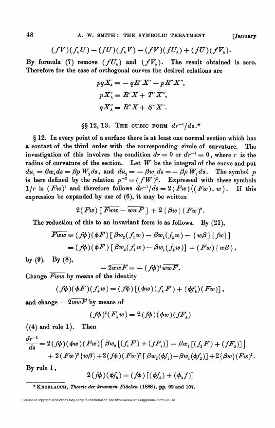
(fV)(fkU) - (fU)(fkV) - (fV)(fUk) + (fU)(fVk).

By formula (7) remove (fUk) and (fVk). The result obtained is zero.

Therefore for the case of orthogonal curves the desired relations are

pqXk = - qR'X' -pR"X",

I>X'k = R'X+ TX",

qX'k = R"X+ S"X'.

§§ 12, 13. The cubic form dr~l/ds*

§ 12. In every point of a surface there is at least one normal section which has

a contact of the third order with the corresponding circle of curvature. The

investigation of this involves the condition dr = 0 or dr~l = 0, where r is the

radius of curvature of the section. Let IF be the integral of the curve and put

dux = ßw.2ds = ßp W2ds, and du2 = — ßwxds =— ßpWxds. The symbol p

is here defined by the relation p~2 = ( fW)2: Expressed with these symbols

1/r is (Fw)2 and therefore follows dr~l¡ds = 2(Fw)((Fw), w). If this

expression be expanded by use of (6), it may be written

2(Fw)[F^w~-wwF] +2{ßw}(Fw)2.

The reduction of this to an invariant form is as follows. By (21),

Ï^W = (f<p)(4>F) [ßw2(fw) - ßwx(f2w) - {wß } {fw}]

= (f<t>)(4>F)[ßw2(fxw)~ ßwx(f2w)] +(Fw){wß},

by (9). By (8), _ _

— 2wwF= — (fpfwwF.Change Fww by means of the identity

(f<p)(<t>F)(fkw) = (ßp) l(<pw)(fkF) + (<ffk)(Fw)] ,

and change — 2wwF by means of

(f<p)2(Fkw) = 2(f<p)(<pW)(fFk)

((4) and rule l). Then

-¿ = 2(f<p)(<pw)(Fw)[ßw2[(fxF) + (fF,)] - ßwx[(f2F) + (fF2)]]

+ 2(Fw)2 {wß}+2(f<p)(Fic)2 ¡ ßw2(<pf1)-ßwx(<f>f2)]+2{ßw}(Fwf.

By rule 1,

Hf*)(¥*) - (/</>) [(#») + (**/)]•KNOBLAUCH, Theorie der krummen Flächen (1888), pp. 92 and 107.



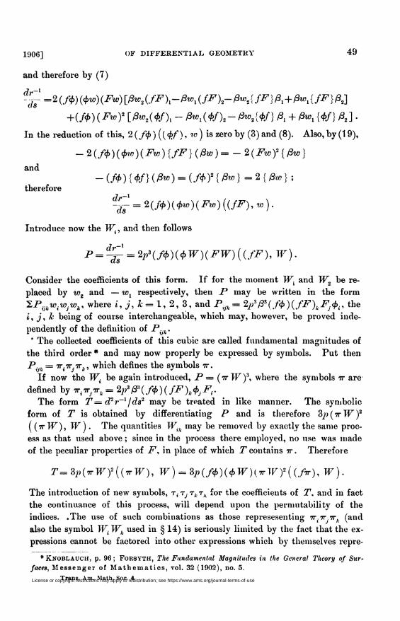
and therefore by (7)

dC=2(f<?)($w)(Fw)[^ßzc2(fF)x-ßwx(fF)2-ßw2{fF}ßx + ßwx{fF}ß2-\

+ (/cp)(Fio)2 [ßw2(4>f\ - ßwx(<pf)2-ßxo2{<pf} /3, + ßwx {<pf} ß2] .

In the reduction of this, 2(f<p)((<f>f), w) is zero by (3) and (8). Also,by(19),

- 2(f4>)(<pw)(Fw) {fF} (ßw)= - 2(Fw)2 {ßw}

and-(#){#} (ßw) = (ff)2 {ßw} =2 {ßw};

thereforefir-1

-dV = 2(f<f>)(4>w)(Ft0){(fF),w).

Introduce now the W¿, and then follows

d<r~l

P = -ji = 2p*(f<P)(<PW)(FW){(fF),W).

Consider the coefficients of this form. If for the moment IFj and IF2 be re-

placed by Wj and — wx respectively, then P may be written in the form

2P,ytwt.w/wt, where i, j, k = 1, 2, 3, and P..,= 2p>ß3(f<p)(fF)kFJ<j>i, thei, j, k being of course interchangeable, which may, however, be proved inde-

pendently of the definition of Pik-

' The collected coefficients of this cubic are called fundamental magnitudes of

the third order * and may now properly be expressed by symbols. Put then

Prk= 7r.ir.ir!., which defines the symbols it.

If now the Wi be again introduced, P = (ir IF)3, where the symbols it are

defined by ir,ir.7Tt = 2p3ß\f<f>)(fF)k<p.Ft. _The form T==d2r~1/ds2 may be treated in like manner. The symbolic

form of T is obtained by differentiating P and is therefore 3^;(irW)2

( ( 7T IF ), IF ). The quantities Wik may be removed by exactly the same proc-

ess as that used above ; since in the process there employed, no use was made

of the peculiar properties of F, in place of which T contains ir. Therefore

T=Sp(irW)2((irW), W) = Zp(f<p)(<pW)(irW)2{(fir), IF).

The introduction of new symbols, t¡ t} ta. tk for the coefficients of T, and in fact

the continuance of this process, will depend upon the permutability of the

indices. .The use of such combinations as those represesenting ir.ir.ir^ (and

also the symbol Wi 1F;. used in § 14) is seriously limited by the fact that the ex-

pressions cannot be factored into other expressions which by themselves repre-

* Knoblauch, p. 96 ; Forsyth, The Fundamental Magnitudes in the General Theory of Sur-

faces, Messenger of Mathematics, vol. 32 (1902), no. 5.

Trans. Am. Matb. Soc. 4License or copyright restrictions may apply to redistribution; see https://www.ams.org/journal-terms-of-use

■50 A. W. SMITH : THE SYMBOLIC TREATMENT [January

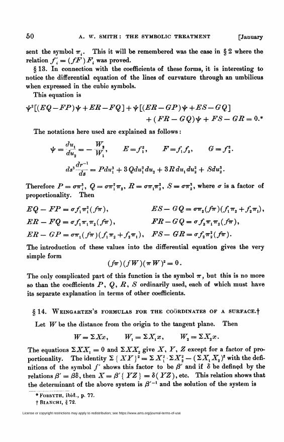
sent the symbol iri. This it will be remembered was the case in § 2 where the

relation f\ = (fF)Fi was proved.

§ 13. In connection with the coefficients of these forms, it is interesting to

notice the differential equation of the lines of curvature through an umbilicus

when expressed in the cubic symbols.

This equation is

■f2[(EQ-FP)ylr+ER-FQ~\ + f[(ER-GP)ylr+ES-GQ]

+ (FR - GQ)ty + FS - GR = 0.*

The notations here used are explained as follows :

ï-wr-ws e-k> *-//.■ G=^dr~l

ds3 -*- = Pdu\ + 2>Qdu\du2 + SRduxdu22 + 8du\.

Therefore P = air3, Q = crrr2xir2, R = crirxir22, S = o-7r2, where a is a factor of

proportionality. Then

EQ-FP = afxir2x(fir), ES- GQ = air2(fir)(fxir2 +f2irx),

ER-FQ = afxirxir2(fir), FR-GQ= a f2irxir2(fir),

ER- GP = airx(fir)(fxir2+f27rx), FS- GR = af2ir\(fir).

The introduction of these values into the differential equation gives the very

simple form

(frr)(/W)(irW)2=0.

The only complicated part of this function is the symbol ir, but this is no more

so than the coefficients P, Q, R, S ordinarily used, each of which must have

its separate explanation in terms of other coefficients.

§ 14. WeINGARTEN'S FORMULAS FOR THE COORDINATES OF A SURFACE.f

Let IF be the distance from the origin to the tangent plane. Then

IF= 2A"x, IF, = 2A>, IF2 = 2A>.

The equations SJJ, = 0 and 2AAT2 give X, Y, Z except for a factor of pro-

portionality. The identity 2 { XY}2 = 2 X2X ■ 2X2 - ( SJ, X2 f with the defi-

nitions of the symbol /' shows this factor to be ß' and if B be defined by the

relations ß' = ßS, then X = ß' { YZ} = 8 ( YZ), etc. This relation shows that

the determinant of the above system is y9'~l and the solution of the system is

•Forsyth, ibid., p. 77.

t Biakchi, \ 72.



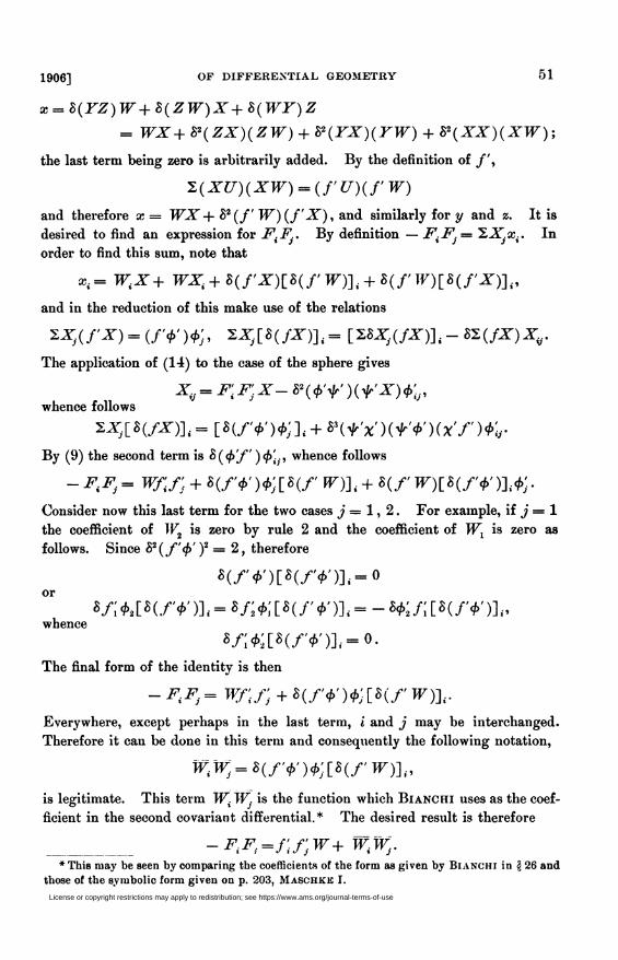
x = 8(YZ)W+8(ZW)X+8(WY)Z

= WX + 82(ZX)(ZW) + o2(rX)(FlF) + 82(XX)(XW) ;

the last term being zero is arbitrarily added. By the definition of /',

Z(XU)(XW) = (f'U)(f'W)

and therefore x = IFA"+ 82(f W)(f X), and similarly for y and z. It is

desired to find an expression for F(F.. By definition — FiF.= 2ATxr In

order to find this sum, note that

xi=IFiX+ WXi+8(f'X)[8(f'W)]i + 8(f'W)\_8(fX)]i,

and in the reduction of this make use of the relations

ZX(f'X) = (f'cp' )</>:, SZ[i(/J)]i= [2SXy(/X)]i-S2(/X)Xr

The application of (14) to the case of the sphere gives

x.. = f: f. x- 82(<p'V)(yx)$\},whence follows

2A;.[S(/x)]<=[8(/>')<P;]j + 83(tV)(^>')(x'/')^-

By (9) the second term is 8(<j>'f )<£¿., whence follows

-FF= Wf'J[ + 8(f'cp')<P'j[8(f'rV)]i + 8(f'W)[8(f'<P')-]i<P'..

Consider now this last term for the two cases ^'=1,2. For example, if j = 1

the coefficient of Wt is zero by rule 2 and the coefficient of IF, is zero as

follows. Since 82(f'<p')2 = 2, therefore

«(/>')[«(/'*')],- »or

SAUHf'tl^ * f WIH f'<?')]<=-WJliHf4>')lnwhence

8/;^[S(/>')], = o.

The final form of the identity is then

-FF= Wf'if'j + 8(f'^)^\_8(f'W)-]i.

Everywhere, except perhaps in the last term, i and j may be interchanged.

Therefore it can be done in this term and consequently the following notation,

WiWJ = 8(f'<P')(p'J[8(f'W)]i,

is legitimate. This term IF; IF^. is the function which Bianchi uses as the coef-

ficient in the second covariant differential.* The desired result is therefore

_ -FiFl=fif'.W+ WtWj.•This may be seen by comparing the coefficients of the form as given by Bianchi in \ 26 and

those of the symbolic form given on p. 203, Maschke I.


52 A. w. smith : the symbolic treatment [January

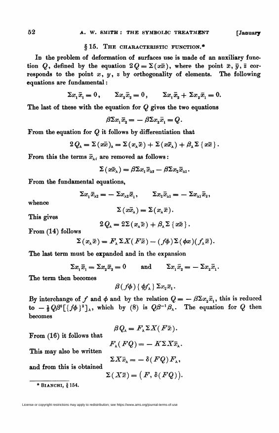
§ 15. The characteristic function.*

In the problem of deformation of surfaces use is made of an auxiliary func-

tion Q, defined by the equation 2Q = 2(xx), where the point x, y, z cor-

responds to the point x, y, z by orthogonality of elements. The following

equations are fundamental :

2x1x1 = 0, 2x2x2 = 0, 2x1x2 + 2x2x\ = 0.

The last of these with the equation for Q gives the two equations

j82x,x3 = — ß'Zx2xx = Q.

From the equation for Q it follows by differentiation that

2ÇA = 2(xx)A = 2(xAx) + 2(xxA)+/3A2{xx}.

From this the terms xki are removed as follows :

2 ( xxA ) = ß2xx xkî — /32x2 xA1.

From the fundamental equations,

2.X, XA2 = — 2,XX2X[, 2,X2XA1 = — 2xA1X2,

whence

2(xxA) = 2(xAx).

This gives2ÇA = 22(xAx) + /3A2{xx}.

From (14) follows

2(xAx) = FkZX(Fx) - (/</>)2(<¿>x)(/Ax).

The last term must be expanded and in the expansion

2xtx, = 2x2x2 = 0 and 2xtx2 = — 2x2X!.

The term then becomes

By interchange of f and <f> and by the relation Q = — ß1x2xx, this is reduced

to -hQß2[{f<l>}2~\^ which by (8) is Qß~lßk. The equation for Q then

becomes

ßQk = Fk^X(Fx).From (16) it follows that

Fk(FQ)=-KÏXxk.This may also be written

ZXxk=-8(FQ)Fk,and from this is obtained

_ Z(Xx)=(F,8(FQ)).

* Bianchi, \ 154.



The left member is evaluated by removing X{ by (15) and the summations by

the fundamental equations. The result is

(F,8(FQ)) = -(fF)2Q.

It is now desirable to express this relation without the Use of the expressions

FtF.k and by means of the symbols /' instead of /. The change is made as

follows :

(F, 8(FQ)) = 8(F, (FQ))+(FQ)(F8),

(F, (FQ)) = -FFQ +^QF+(FQ) {Fß},

and by (6) FQF= QFF.

The expression QFF is simplified by the Codazzi formulas, viz.,

(FFk)=-(f<p)(F<p)(Ffk).

The terms containing 8Fk(FQ.) are changed as follows:

8Fk(FQs) = \83(f'4>')2(FQj)Fk by (8)

= 83(f'<p')(f'F)(<p'Q.)Fk

by means of (4) applied to (f'<p')(FQj) and then rule 1.

The symbols y and (p occur in the terms (f<f>)(F<f>)(Ffk) introduced by the

Codazzi formulas. They may be removed by the relations f. = — 8(f'&)<&.,

<p.= -S^"^)^. These lead to the relations (f<f>) = 8(f'<p') by rule 1 and (16),

(F<p) = -8(<pl'V)(FV),znd(Ffk)=-[8(f'®)]k(F)-8(f')(Fk).

As a result of these changes there is introduced a term

-83(f'<p')(<p'V)(FV)[-ßQ2[8(f'<S>)]x(F)

+ ßQlHf'*MF*)~ßQtt(f'*)(F*l) + ßQl(f'*)(F*t)\.

To the expressions (<p"V )(F<P) and (<p"V)(F&k) which occur in this term

apply (4) and use the relation 8(F"^)2 = 2. These reductions lead to

{F,8(FQ)) = 83(f'<P')(f'F)[ßFx(<p'Q2)-ßF2(<p'Qx)]

+ 8(FQ){Fß}-82(f<p')(<p'^)[-ßQ2[8(f'^)-]x+ßQx[8(f'^)]2\

V(A<t>')(A®)l- 0Q*H+'*i) + 0&«<*'*,)] + (FQ)(F8).

If 8(FQ){ Fß} and (FQ){Fß} be multiplied by \82(f'<p')2, they can be

written (by (4) and rule l) in the forms 83(f'<p')(f'F)(<f>'Q){Fß} and

^(.f'<p')(AF)(<p'Q)(F8) respectively.In the third and fourth terms <í> is to be replaced by F, and in the third f

and <p' interchanged. If now for [8(<p'F)']k one substitutes



M<t>'F) + 8(cf>'kF) + 8((p'Fk) + 8{<p'F}ßk

and groups the terms according to (7), the result is the desired relation. In this

final reduction the coefficients of (Q8) and (Qß) are zero. Therefore

8(F,8(FQ))=83(f'<t>')(f'F){F,(<p'Q)).

The expression (fF)2 when transformed by the elimination of / becomes

8(f'F)2 and the characteristic equation is accordingly

83(f'cp')(f'F)(F,8(4,'Q)) = -82(f'FyQ.

Into this equation the symbols Q¡Q. are easily introduced. By definition

Q.Q.= — à(f'4>')f'i[^('A'Q)1 ■ an(l *ne equation may therefore be written

(FQ)2 = -(f'F)2Q.

It has been proved that if IF be the distance from the origin to the tangent

plane, — FiFj z=f'if'jW+ WfW,. If now the symbols F be removed by this

relation, the characteristic equation becomes

(f'Q)2W-r(f'W)2Q = (f'<p')2WQ-(WQy.

It is to be noted that the functions IF and Q enter into this equation symmet-

rically and from this follows the theorem : *

If S0 denote the envelope of the planes 2Ax = IF and if Q be the charac-

teristic function for an infinitely small deformation of the surface S, then

is W the characteristic function for an infinitely small deformation of the

surface Sg.§ 16. Rectilinear congruences.

The analytical definition of rectilinear congruences is as follows : The entire

system of rays is cut by a surface S and that point (or one of them if there are

more than one) in which the ray cuts the surface is taken as the origin of each

ray. The surface S is defined analytically by a curvilinear system of coordi-

nates («j, u2) and any ray is determined from its origin x, y, a and its direc-

tion cosines X, Y, Z, all expressed as functions of ux and u2. The spherical

image of any ray is the point X, Y, Z on the sphere. Only in special cases

are the rays perpendicular to S.

The forms der2 = 2á*AT2 and "EdxdX are fundamental. The first of these is

the Gaussian arc form, but since the first fundamental form is not here consid-

ered, the accents on the symbols for da2 and on ß' will be omitted. Whenever

these are introduced again, every ( ) must be replaced by 8 ( ). The symbols

used are AAj— 2ATiATand FiF = 2ATx.. It is to be noticed that the symbols

Fi and F. are not interchangeable in the general case and that it takes a product

of the two for the actual meaning.

•Bianchi, §155.



Let now cos A, cos/*, cosí; be the direction cosines and dl the length of the

common perpendicular from (uxu2) to the consecutive ray (ux + c?m,, u2 + du2).

The direction cosines of the two rays are X, Y, Z and A + dX, Y-\- dY,

Z+dZ. Then 2X cos A = 0 and 2 ( X + dX ) cos A = 0 and therefore

cos A : cos ¿i : cos i> = (YdZ - ZdY) : (ZdX- XdZ) : (XdY - YdX).

From the equations 1XXi = 0 follows X= ( YZ). Let IF be a curve on S,

and p be defined as before. Then from the notations in use

YdZ-ZdY = (fX)\fxdux +f2du2] =P(fX)(fW).

Therefore cos A : cos u : cos v = (,/A")(/IF) : (fY)(fW) : (fZ)(fW) and

the solution of this is cos A = p2(fX)(fW), etc.

The length of the line between the two rays is

dl = 2 cos Xdx = P3(fF)(fW)(FW).

If now r be the distance along a ray from its origin to its intersection with dl,

then it may be proved that

r=-^¿=-P2(FW)(FW).*

§ 17. Principal curves.

Introduce now conditions which in form of expression are similar to those

imposed for lines of curvature. Let U and F be curves which satisfy the

equations (fU)(fV) = 0 and (FU)(FV) + (FU)(FV) = 0. These ave

the principal curves. Let rx and r2 be the values of r for rays whose origins

are on these curves. Then rx=-p2(FU)( FU ) and rt = - q2 ( F V ) ( FV ).

The first of the conditions on U and F may be written V. = m ( fU )f. and by

substitution of this it follows that

r2=-p2(fF)(<pF)(fU)(<pU).

Consider now three rays, one the original ray at the intersection of U and F,

the two others near to this, one on U and one on W, a curve copunctual with

£7 and V. From the original ray to each of the others there is one line which

is perpendicular to both. Let m be the angle between these twp lines. Then

by the formulas proved above (the subscripts referring to the curves)

cos . = 2 cos A.cos K=PÎAW)(*U)ï(fX)(4>X) =p(fW)(fU_)}/(fwy V(fwy

by (17) and (9). From this follows, as in § 2,

P2(fW)(<t>w)(fU)(4>u) p2(uwy-jjWj- ~(fwT'

•Bianchi, §137.


56 A. W. smith: the symbolic treatment [January

Form now the expression — (r, cos2 a> + r2 sin2 a>) as a function of U and IF.

Except for the difference in notations and the conditional equations, this prob-

lem is that of Euler's formula and may be proved by exactly the same method

as was employed in the former problem (§ 5). The result is Hamilton's equa-

tion, r = »• cos2 <o + r2 sin2 eo, where r has the value pertaining to the curve IF.

The maximum and minimum properties of r, and r2 may be proved. Suppose

r2 > i",. Then from Hamilton's equation

r — rx = ( r2 — r, ) sin2 a>,

r — r2 = ( rx — r2 ) cos2 a>

and therefore rl<r<r2. The intersection Lx of the ray (ux, u2) and the

common perpendicular between this ray and the consecutive ray on U is called

a limit point. A similar point, L2, exists for the curve V. The angle between

these two perpendiculars is obtained from the formula for cos &> if IF is replaced

by F. The numerator in that case has the factor (fU)(fV). Therefore the

lines are orthogonal.

In the exceptional case where the coefficients of the two forms are propor-

tional, the notations give F. = kf , F. — Tcf, and therefore r = r, = r2= — kk.

Any curve IF(m,, wj = 0 on S determines a system of rays which form a

ruled surface. Principal surfaces will be those determined in this manner by

the principal curves U and F. The differential equation of the principal sur-

faces is found from the conditions on U and F and is

(A) [_(FW)(fF) + (FW)(fF)-](fW) = Q.

§ 18. The quadratic in r.

Owing to the differences in notation the derivation of this equation cannot be

referred back to the work on the similar problem in the cuse of the radii of

curvature.

Consider first —(»', + r2). This may be reduced by'repeated applications of

(4) to p2 q2(fF)(fF) ( VU)1. But since for U and F sin2 U). Aside from the factor p2q2 this is

(FV)(4>U)[(F4>)(VU) + (FU)($V)]or

(FV)(4>U)[(F<Ï>)( VU) + (FU)'(<t>V)].

From the addition of these two expressions together with the second condition

on ¿/and F follows

2rxr2=p2q2(F®)(FV)(U)(VU)+p2q2(F)(FV)(i>U)(VU).


1906] OF differential geometry 57

The pairs of symbols F, F and 4>, í> may always be interchanged and therefore

2p2q2(F®)(FV)(®U)(VU) = p2q2(F®)(F<&)(VU)2=(F<î>)(F<$).

By (4),

p2q2(F<S>)(FV)($U)(VU)=(F<l>)(F4>)-P2q2(F®XFU)(ö>V)(VU).

From these results may be written

4rxr2 = (F)(F<§) + 2(F$)(F<Í>) - 2p2q2(F<t>)(FU)($V)(VU).

In every term, except perhaps the last, F and F, 4> and <ï> may be simultane-

ously interchanged, and therefore also in the last. Thus

- 2^2q2( F<S> ) ( FU) ( $ F)( VU) = - 2p2 q1 ( F$ ) ( FU) ( <ï> F) ( VU)

= -2p2q*(<PF)($U)(FV)(VU)-(F$)(F<ï>)

by the process of (9). The substitution of this result reduces the relation to

4r, r, = ( F4> ) ( F Ö> ) + ( Fi )( F& )

and the desired equation is

(B) 4r2 + á(fF)(fF)r+(F<í>)(F$) + (F$)(F<l>) = 0.

§ 19. Developable surfaces.

Developable surfaces are defined as those for which the consecutive rays

intersect. If IF defines a curve such that the corresponding system of rays

form a developable surface, then must IF satisfy the differential equation

dl = 0, that is, IF must satisfy

(O) (fF)(fW)(FW) = 0.

There are then through each point of S two developable surfaces, real or imagi-

nary. Consider now two curves IF and T which are defined by the relations

(JW)(fT) = 0and (FW)(FT) = 0 [or (FW)(FT) = 0]. These twoconditions are distinct from those for principal curves, the second condition in

this case requiring more than the corresponding condition for principal curves.

From the first of these conditions follows IF; = n(fT)f. or Ti = m(fW)fi.

The substitution of either of these relations into the second condition shows that

the surfaces defined by these curves are developable surfaces.

Let the ray through a point P meet the cuspidal edges of these surfaces in

the points Px and P2, which are called foci of the system. Let also px and p2

be the distances PPX and PP2 respectively. If by f, t¡, % are denoted the

coordinates of the cuspidal edge, then f = x + pX, etc., and since the ray is

tangent to the cuspidal edge at the focus, it follows that dx + pdX = XX,



where A is a factor of proportionality. This last relation may be written

(x W) +p( XW)=XX and therefore for j =1, 2. 2 X (x W) +pZX.(XW) = 0.

This equation expressed in symbols is (FW)Fj + p(fW)fj= 0. Let the

value px go with W and p2 with T. These give rise to the following system of

equations :

1) Fx(FW) + PlA(fW) = 0, 3) <t>x(<S>T) + p2<px(<pT) = 0,

2) F2(FW) + PlA(fW) = 0, 4) $>2(<bT) + p2<p2(<pT) = Q.

From the multiplication of 1) by 4) and 2) by 3) follow

Fx<P2(FW)(ÏT) = Pxp2fx<p2(fW)(<f>T),

F2ix(FW)(ÎT) = pxp2f2<px(fW)(<pT).

The subtraction of these two equations and the interchange of equivalent

symbols gives

2pxp2 = (F4>)(F$).

Now multiply equation 1) by (<j>T)<p2 and 2) by (tpT)cpx, subtract them, and

then do the same for 3) and 4). With proper changes of notation this gives

the two equations :

(F<p)(<pT)(FW) + Px(f<p)(<t>T)(fW) = 0,

(F<p)(<pW)(FT)- p2(f<p)(<pT)(fW) = Q.

From these equations is obtained px + p2 = — (fF)(fF), and therefore the

desired quadratic is

(D) 2p2 + 2(fF)(fF)p + (F)(Fà) = 0.

It is at once evident that rx + r2 = px + p2.

The point midway between the foci, and so midway between the principal

points also, is called the mid-point and its locus is the mid-surface.

The four equations (.4), (B), (C), (D) are here given with the complete nota-

tion. In the next section the full form is needed.

(A) o* {(FWyj'F) + (FW)(f'F)-] (/' IF) = 0,

(B) ir2 + W(f'F)(fF)r + 82(F)(FÔ>) + 8*(FÏ>)(F<Î>) = 0,

(C) 83(f'F)(f'W)(FW) = 0,

(D) 2p2 + 282(f'F)(f'F)p + 82(F<S>)(FÖ>) = 0.



§ 20. The coincidence of the focal surfaces.*

It may be shown that if the two focal surfaces coincide the cuspidal edges

unite into a system of asymptotic lines. Assume this to be the case and choose

for S the combined focal surfaces. Since now the ordinary surface elements

enter into the work, the symbols / and /' are to be distinguished. Let U be the

system of asymptotic lines, F their orthogonal trajectories. Then (FU)2 = 0.

Furthermore let X', Y', Z' be the direction cosines of the tangent to the curve

U; X", Y", Z" of the tangent to F; and X, Y, Z of the normal to S. Then

from § 11,

X'k = RkX+TkX"where

X'=p(xU), X" = q(xV),etc.,

Rk = p(FU)Fk, Tk = mt(f<p)(<pU)(fU)k.

These equations involve only the orthogonality of U and V. According to the

hypothesis X', Y', Z' are the direction cosines of the rays. Expressions are

next to be found for the rectilinear congruence symbols. In this computation

it is to be noted that Rk and Tk have actual meaning and are not symbols in

the technical sense.

From the" relations 2X2 = 2X'2 = 2X"2 = 1, 2X"A" = 2Ax. = 0,

2X"x). = 22(x V)Xj = q( fV)fj it follows that

/:/> = 2x:x; = i?<^+rir>, FiFj = ^x\xj = q(fV)TifJ.

The next step is the investigation of the quadratic for r, viz :

4r2 + 482(f'F)(fF)r + 82(F<P)(FÏ) + 82(FÏ)(Fi) = 0.

Consider now the coefficient of r, which may be written

*82pqmt(fF)(fV)(FU)(W)( + U){(<pU),R).

(In the reduction to this form remove FiF. first, tbenf^f'j.)

Since (fF)(yTrU) = (^F)(fU) + (FU)(f^), the above expression is

zero on account of the conditions (fU)(fV) = 0 and (FU)2 = 0.

The expression (F$>)(F<P) + (F® ) (F® ) = 0 may be written

q2(fV)(<t>V)[(TT)(f<p) + (T<p)(fT)-].

The first term is zero and the second is — a2[(/F)(/77)]2, which, by the re-

moval of T and the usual reduction of the number of symbols, becomes

-vlq2[(fV){(fU),v)}2.Consider now ß2ß'~2= (RT)2, which is easily derived from the notations.

In the expression for (RT) apply (4) to (<pU)(F, (fU)). This reduces

* Bianchi, \ 142.


60 A. W. SMITH : THE SYMBOLIC TREATMENT OF GEOMETRY

(RT) to pmt(f<p)(<pF)(FU) ( U, (fU) ), and if this expression be squared

and (4) be applied to (FU)(x&), the result is

(RT)2=p2m2t2(f<p)(^)(<pF)(Fi)(xU)(iU){U,(fU)){U,(Û)).

Apply the method of (9) to (F$>)(cf>F)(U), and in the result put

m(f<p)(<pU) = (fV) and m(^x)(XU) = (^V).

This gives as a final result ß2ß'~2= -p*t2(fV)(U, (fU))K. If these

results are now substituted in the quadratic for r, and reductions made by use

of the relations mq=p, mt = p2, and ß8 — ß', it follows that 4p2 = — ÜT.

Whence the theorem :

If the two focal surfaces coincide, then 4Í*2 = — K, or in other words, the

distance between the principal points is \¡V — X.

Hamilton, N. Y.

Documents

THE SYMBOLIC TREATMENT OF DIFFERENTIAL GEOMETRY* · 2018-11-16 · THE SYMBOLIC TREATMENT OF DIFFERENTIAL GEOMETRY* BY ARTHUR WHIPPLE SMITH In this paper certain theorems of differential