Embed Size (px)
Citation preview

The Swedish Housing Market An empirical analysis of the real price development on the Swedish housing
market.
NILS LANDBERG
Master of Science Thesis
Stockholm, Sweden 2016
The Swedish Housing Market
An empirical analysis of the price development on the
Swedish housing market.
Nils Landberg
Master of Science Thesis INDEK 2015:48
KTH Industrial Engineering and Management
SE-100 44 STOCKHOLM

3
Abstract
This thesis discusses the real price development on the Swedish housing market and
the effects by qualitative variables. The housing market shows signs of being
overpriced and this paper investigates if these qualitative values significantly effect the
real price development.
Valueguard Corporation has supplied Price development data. Focus magazine has
supplied data regarding a large dataset for Swedish municipalizes which measures
which state of quality of living prevailing in the investigated area.
Empirical results show that qualitative variables and increased population have a
positive effect on the real price development. Increased cost of interest rates has a
significant negative effect on the price development. Increased amortizing rates and
interest rates are assumed to slow down an unsustainable price development.
Key-words: The Swedish housing market, Price bubble, Significance level, Causal
relationship, Estimation
Master of Science Thesis INDEK 2015:48
The Swedish Housing Market
An Empirical analysis of the price development on the
Swedish housing market.
Nils Landberg
Approved
19/2-2016
Examiner
Kristina Nyström
Supervisor
Stefan Fölster

4
Acknowledgements
I would like to thank my supervisor Stefan Fölster for helping me structure this Master
thesis and supplying me with my contact at Valueguard Corporation, Lars-Eric
Eriksson, CEO. Furthermore I would like to thank Mr. Eriksson for supplying me with
the data set of the price development in Sweden, making this paper possible. I would
also like to thank MSc. Viktor Sundvall for increasing my knowledge in VBA-
programming. Finally I would like to thank my friends and family for creating the
perfect conditions for writing this Master thesis.

5
Table of Contents 1. INTRODUCTION .......................................................................................................................................... 6
1.1 Background ....................................................................................................................................... 6 1.2 Aims of the thesis ............................................................................................................................ 6 1.3 Price development on the housing market ........................................................................... 7 1.4 Economic Sustainability .............................................................................................................. 9
2. THEORY ..................................................................................................................................................... 10 2.1 Previous research and contribution for the future ......................................................... 10 2.2 Price bubbles on the housing market ................................................................................... 14 2.3 The housing market ...................................................................................................................... 15 2.4 The Market Supply ....................................................................................................................... 16 2.5 The Housing market in United Kingdom ............................................................................ 17 2.6 Why and when prices would fall ............................................................................................. 17 2.7 The interest rate ............................................................................................................................ 18 2.8 The lending ratio ........................................................................................................................... 18 2.9 Why a price increase is a problem ........................................................................................ 19 2.10 The mortgage market .................................................................................................................. 20
3. DATA AND VARIABLES ......................................................................................................................... 22 4. METHOD.................................................................................................................................................... 26
4.1 Limitations for the model .......................................................................................................... 26 4.2 Division ............................................................................................................................................. 27 4.3 Models ............................................................................................................................................... 27 4.5 Empirical expectations ............................................................................................................... 29
5. RESULTS ................................................................................................................................................... 31 5.1 The Hausman test ......................................................................................................................... 31 5.2 The Xtabond2 model .................................................................................................................... 31
6. ANALYSIS ................................................................................................................................................. 32 6.1 The Arello-Bond model .............................................................................................................. 32
7. DISCUSSION ............................................................................................................................................. 33 7.1 Why suppliers doesn’t produce more housing .................................................................. 34 7.2 Fokus ranking................................................................................................................................. 34
8. CONCLUSION AND SUGGESTIONS ...................................................................................................... 35 8.1 Future research ...................................................................................................................................... 36
9. REFERENCE .............................................................................................................................................. 37 10. APPENDIX 1 ........................................................................................................................................... 41
10.1 The “quality of living” variable ranking system.................................................................... 41 11. APPENDIX 2 ........................................................................................................................................... 43
6
1. Introduction This chapter introduces the incentives with this paper, discussing the price development
on the Swedish housing market and gives an insight for which problems will be
discussed. The paper starts of by discussing the housing market in Sweden, explaining
the problematic with a developing real price market.
1.1 Background
The real price development on the Swedish market continues to increase, which grows
interest in how the market works and which parameters, makes the prices change.
Previous research concludes that an open housing market should be affected by cost of
interest and supply. As the Swedish population has been centralizing towards larger
cities, increasing the demand for housing in these parts. Then the opposite should
rationally apply for the municipals, which people are moving from. The population
growth is therefore an interesting parameter to include in the model. These effects
however doesn’t seem to revile the entire story which yielding interest in how
qualitative variables as quality of living are reflected in the price development and if
they are significant (Figure 1, Birch Sorensen, 2013).
1.2 Aims of the thesis
The increased cost of housing prices in the United States and the correlated effects on
the American populations’ quality of living is analyzed by Roxanne Ezzet-Lofstrom in
2004. Ezzet-Lofstrom concludes that there is a correlation between increasing housing
prices and the inhabitants’ quality of living. The initial theory of Roxanne Ezzet-
Lofstrom was that increased housing prices should have a negative effect on the quality
of living as the increased cost reduces the bundle of goods from a monthly income. The
results in her paper however were contradictory to this theory as they indicated that the
quality of living instead seemed to have a positive effect on the housing price market.
This thesis aims at investigating if this effect is applicable on the Swedish housing
market and if so, how it affects the housing price development. (Ezzet-Lofstrom, 2004).
The thesis aims at concluding how qualitative values as the quality of living affects the
pricing development for housing over time. Defining the effects of these qualitative
variables will yield an insight in how the future development on the housing market
will change.
Deriving a model with respect to qualitative parameters into a quantitative model of the
housing market will also help on predicting where to expect higher returns on capital
investments on the housing market. This will also enable mortgage institutes to revalue
their risk calculations of their return on investment with respect to the aspect of quality
of living for a given area.
The empirics incorporate the results of an annual extensive semi-qualitative ranking
system concluded by the Fokus time script. This variable combines variables that are
hard to define quantitatively in a ranking system. For example “how well people like
their municipal” is included in this ranking. It is believed that the social environment is
important when purchasing housing and these values should then reflect in to the price
development. This thesis also aims on describing the complexity of the market and
strategies for how a price development can be controlled and how price changes may
differ depending on the municipal size.

7
The empirical results will be compared to economic theories and later on it will be
discussed if there is a market failure and how economic policies can adjust for this for
the future.
The main idea behind this paper is to understand if qualitative parameters yield
significant effects on the real price variations around in Sweden to be able to make
forecasts for the future price development and to analyze which social aspects that are
reflected in the price. This paper discusses how the Swedish housing market is affected
by a semi-qualitative variable for a municipality’s wellbeing through the Xtabond2-
model (Shiller, 2007).
The empirical analyses are made to analyze and minimize the risk on the real estate
market and to try and explain the variation for the real price development in Sweden.
1.3 Price development on the housing market
This thesis aims at describing how qualitative parameters affect the price development
for housing in Sweden. The central bank of Sweden concludes that the large increase
in housing prices can be derived into fundamental aspects as people continuously move
into the larger cities. This implies that the price increase should be centralized towards
the largest municipalities in Sweden (Flam, 2014).
The housing market consists of products that may not need to follow the basic
economical concepts. There is supply advancement on the market as housing is a
necessary requirement for people having a place to live, which is a basic necessity for
the society to hold. As the population is continuously growing, the demand for houses
and apartments may be somewhat unsaturated in some districts. This could yield an
inefficient price market with price surpluses exceeding the efficient price equilibrium
level (Birch Sorensen, 2013).
My expectations is that there is a centralized monopolistic competition on the housing
market as there tend to be more people attracted to live in the larger cities and this could
reflect on the price development. This initial belief is based on that larger cities tend
to offer greater job possibilities and has a higher population growth yielding increased
high demand and hence higher prices (Birch Sorensen, 2013).
A common belief of the housing market in Sweden is that prices will always increase,
which yields support from Figure 1. This reality is not able to continue, which will be
discussed later in this paper. (Andersson, 2014)
8
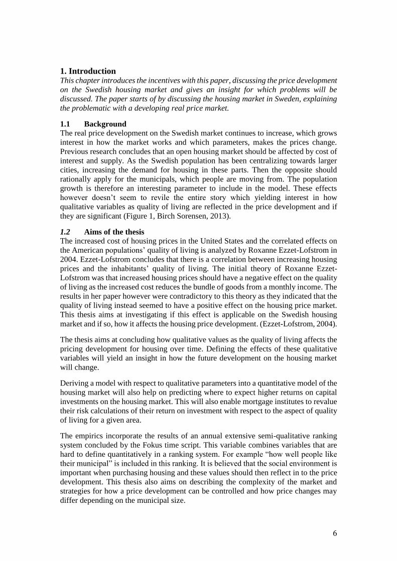
Figure 1: The average price index development between 2005-2013 in Sweden (Valueguard, 2014)
To analyze the price index development in Sweden, the Swedish municipalities are
evenly divided into 4 groups1. The groups are based on the population from 2005 where
the largest municipals are in group 4 and the smallest municipalities are in group 1.
From analyzing Figure 2, one can see that the largest municipals have had the lowest
relative price index growth rate. The results generate a question of which other
parameters that effects the price development.
Looking at Figure 1, you are able to see the relative price index development between
the years 2005-2013. This shows of an average price increase of 200% during the past
decade around in Sweden (Andersson, 2014).
Average Price Increase
Time
Figure 2 the price development of the Swedish municipals divided into 4 population size groups. (Valueguard,
2014)
1 The groups are divided by population sizes at year 2005 into Group 1: Populations larger than 60000, group 2 populations
between 30-60 000, group 3 populations between 22- 30 000, group 4 populations smaller than 22 000 inebriants
Percent
Percent
Month-Year

9
1.4 Economic Sustainability
A continuous real price development on the UK housing market is an unsustainable
economic development if the real income development per capita doesn’t follow.
House prices have increased rapidly during the last decade. As real house prices go
up, people increase their amount of mortgages and people become more exposed of
interest rate fluctuations (Bank of England, 2004).
The Swedish population is continuously spending larger parts of their real income on
housing. This continuous change in allocating private resources is not economic
sustainable as people need to spend their income on other goods. The effects and
implications of this is discussed in this paper (SCB, 2011).
10
2. Theory This chapter defines the problem of the current price development. Discussing the
phenomena of price bubbles, the mortgage market and the macroeconomic aspects of
a sudden fall on the real estate market.
2.1 Previous research and contribution for the future
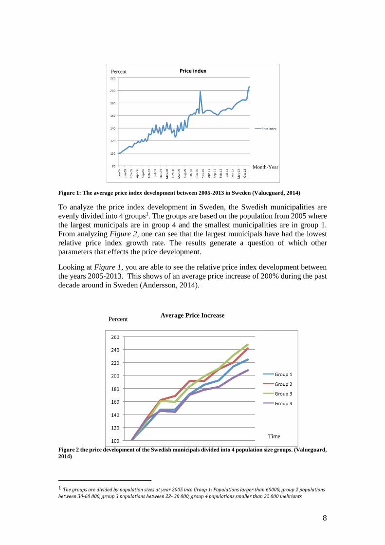
The housing prices in Sweden are currently at a historically high real price level.
Sprensen published a report on this matter for the Swedish institute of finance in 2013.
Sorenson’s report aims at describing the current situation on the Swedish housing
market to conclude if the market is overvalued. Figure 3 describes the average real
price development for housing prices between 1952-2012. Prices have tended to
fluctuate around a long-term equilibrium level between 1952-2000 but since then, real
prices have increase rapidly. Sorensen’s report also concludes that the price-level
increase has been especially strong in the centralized larger cities in Sweden (Sorensen,
2013).
The housing real price increase trend is a phenomenon that doesn’t only apply to
Sweden but has been found in several other OECD countries concludes Sorensen.
Shiller discusses the markets real price increase in USA and if there is a long-term trend
in an increased price level or if the market is building up a price-bubble (Shiller, 2007).
Shiller finds that there has been a long-term equilibrium level and believes that the
relationship should be constant over time.
Real housing prices in Sweden, index value at 100%, year 1952
Figure 3 Real house price developments in Sweden 1952-2012 (SCB, 2014)
Percent
Year
11
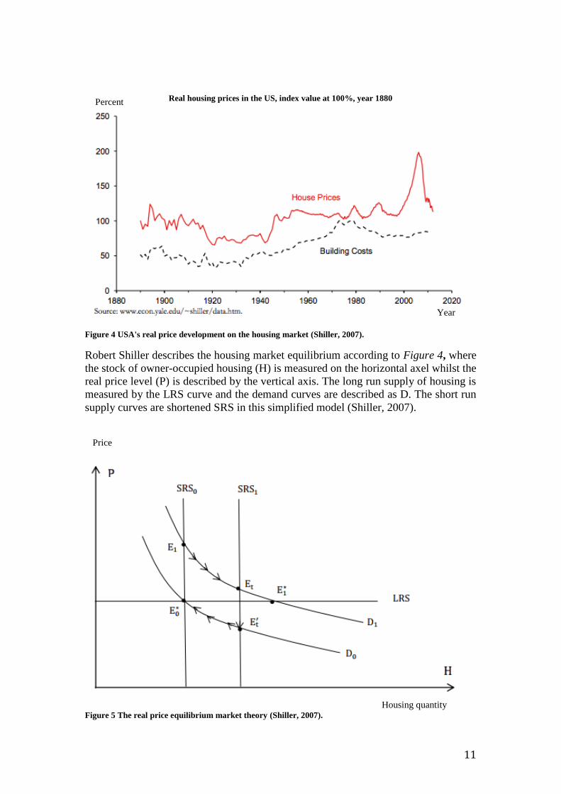
Real housing prices in the US, index value at 100%, year 1880
Figure 4 USA's real price development on the housing market (Shiller, 2007).
Robert Shiller describes the housing market equilibrium according to Figure 4, where
the stock of owner-occupied housing (H) is measured on the horizontal axel whilst the
real price level (P) is described by the vertical axis. The long run supply of housing is
measured by the LRS curve and the demand curves are described as D. The short run
supply curves are shortened SRS in this simplified model (Shiller, 2007).
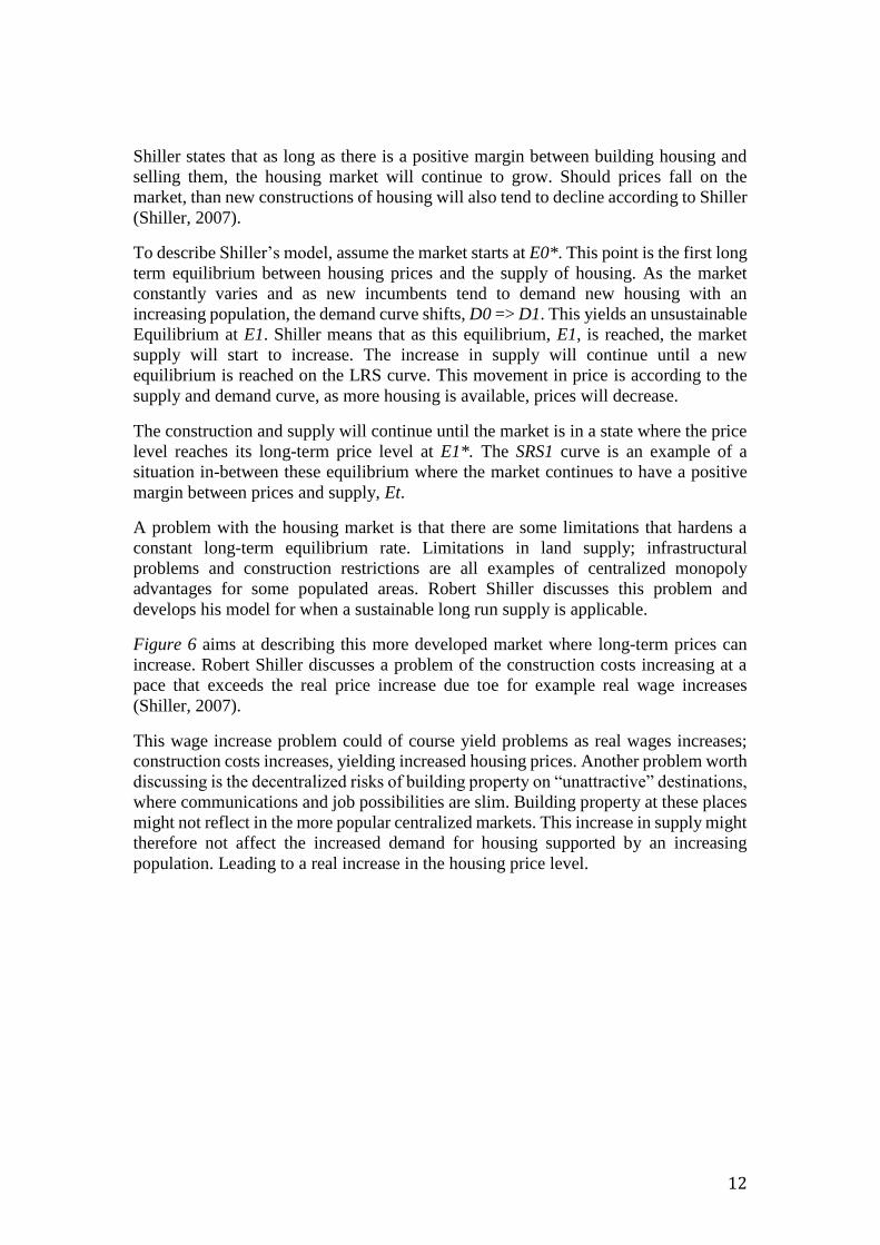
Figure 5 The real price equilibrium market theory (Shiller, 2007).
Year
Percent
Price
Housing quantity
12
Shiller states that as long as there is a positive margin between building housing and
selling them, the housing market will continue to grow. Should prices fall on the
market, than new constructions of housing will also tend to decline according to Shiller
(Shiller, 2007).
To describe Shiller’s model, assume the market starts at E0*. This point is the first long
term equilibrium between housing prices and the supply of housing. As the market
constantly varies and as new incumbents tend to demand new housing with an
increasing population, the demand curve shifts, D0 => D1. This yields an unsustainable
Equilibrium at E1. Shiller means that as this equilibrium, E1, is reached, the market
supply will start to increase. The increase in supply will continue until a new
equilibrium is reached on the LRS curve. This movement in price is according to the
supply and demand curve, as more housing is available, prices will decrease.
The construction and supply will continue until the market is in a state where the price
level reaches its long-term price level at E1*. The SRS1 curve is an example of a
situation in-between these equilibrium where the market continues to have a positive
margin between prices and supply, Et.
A problem with the housing market is that there are some limitations that hardens a
constant long-term equilibrium rate. Limitations in land supply; infrastructural
problems and construction restrictions are all examples of centralized monopoly
advantages for some populated areas. Robert Shiller discusses this problem and
develops his model for when a sustainable long run supply is applicable.
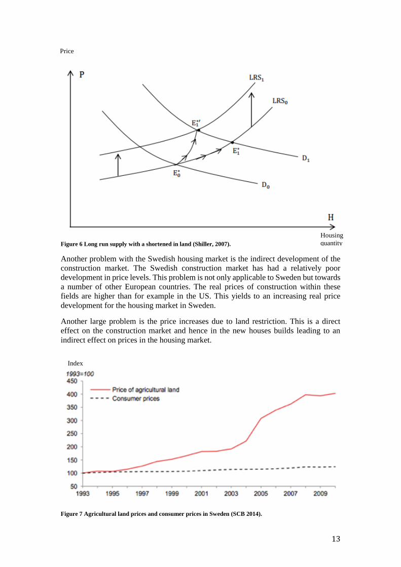
Figure 6 aims at describing this more developed market where long-term prices can
increase. Robert Shiller discusses a problem of the construction costs increasing at a
pace that exceeds the real price increase due toe for example real wage increases
(Shiller, 2007).
This wage increase problem could of course yield problems as real wages increases;
construction costs increases, yielding increased housing prices. Another problem worth
discussing is the decentralized risks of building property on “unattractive” destinations,
where communications and job possibilities are slim. Building property at these places
might not reflect in the more popular centralized markets. This increase in supply might
therefore not affect the increased demand for housing supported by an increasing
population. Leading to a real increase in the housing price level.
13
Figure 6 Long run supply with a shortened in land (Shiller, 2007).
Another problem with the Swedish housing market is the indirect development of the
construction market. The Swedish construction market has had a relatively poor
development in price levels. This problem is not only applicable to Sweden but towards
a number of other European countries. The real prices of construction within these
fields are higher than for example in the US. This yields to an increasing real price
development for the housing market in Sweden.
Another large problem is the price increases due to land restriction. This is a direct
effect on the construction market and hence in the new houses builds leading to an
indirect effect on prices in the housing market.
Figure 7 Agricultural land prices and consumer prices in Sweden (SCB 2014).
Housing
quantity
Index
Price
14
2.2 Price bubbles on the housing market
The housing prices are widely discussed in the media and people are discussing if there
is a price bubble for the housing market that is on the tip of the breaking point. A value
crash for the housing market in Sweden under this era of recovering from a deep
financial crisis could yield tremendous negative effects on the economic society, both
in Sweden but perhaps also have a spreading affect around Scandinavia and maybe
even the Baltic’s and around in Europe (Andersson, 2014).
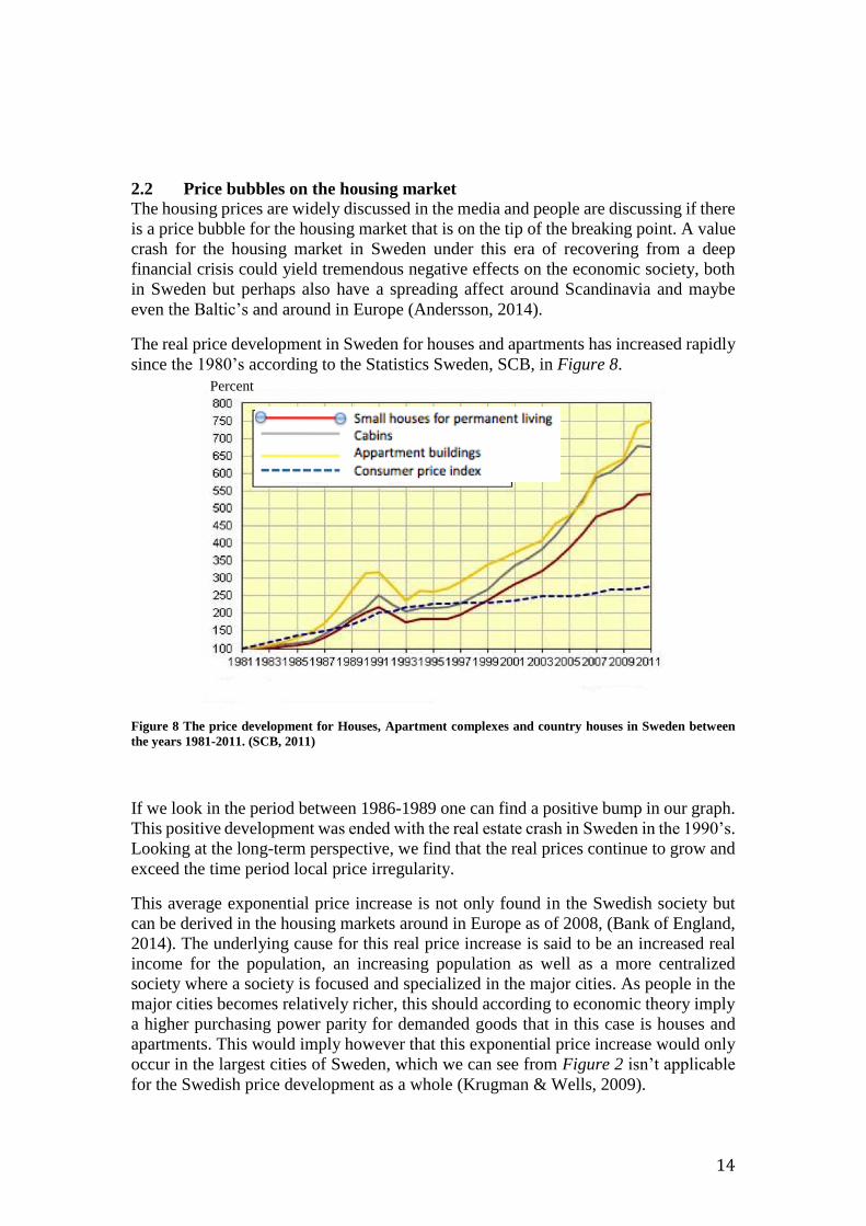
The real price development in Sweden for houses and apartments has increased rapidly
since the 1980’s according to the Statistics Sweden, SCB, in Figure 8.
Figure 8 The price development for Houses, Apartment complexes and country houses in Sweden between
the years 1981-2011. (SCB, 2011)
If we look in the period between 1986-1989 one can find a positive bump in our graph.
This positive development was ended with the real estate crash in Sweden in the 1990’s.
Looking at the long-term perspective, we find that the real prices continue to grow and
exceed the time period local price irregularity.
This average exponential price increase is not only found in the Swedish society but
can be derived in the housing markets around in Europe as of 2008, (Bank of England,
2014). The underlying cause for this real price increase is said to be an increased real
income for the population, an increasing population as well as a more centralized
society where a society is focused and specialized in the major cities. As people in the
major cities becomes relatively richer, this should according to economic theory imply
a higher purchasing power parity for demanded goods that in this case is houses and
apartments. This would imply however that this exponential price increase would only
occur in the largest cities of Sweden, which we can see from Figure 2 isn’t applicable
for the Swedish price development as a whole (Krugman & Wells, 2009).
Percent
15
2.3 The housing market
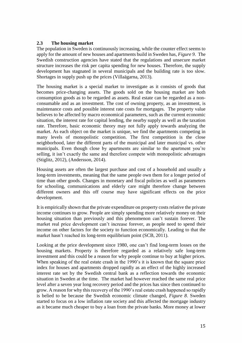
The population in Sweden is continuously increasing, while the counter effect seems to
apply for the amount of new houses and apartments build in Sweden has, Figure 9. The
Swedish construction agencies have stated that the regulations and unsecure market
structure increases the risk per capita spending for new houses. Therefore, the supply
development has stagnated in several municipals and the building rate is too slow.
Shortages in supply push up the prices (Villaägarna, 2013).
The housing market is a special market to investigate as it consists of goods that
becomes price-changing assets. The goods sold on the housing market are both
consumption goods as to be regarded as assets. Real estate can be regarded as a non-
consumable and as an investment. The cost of owning property, as an investment, is
maintenance costs and possible interest rate costs for mortgages. The property value
believes to be affected by macro economical parameters, such as the current economic
situation, the interest rate for capital lending, the nearby supply as well as the taxation
rate. Therefore, basic economic theory may not fully apply towards analyzing the
market. As each object on the market is unique, we find the apartments competing in
many levels of monopolistic competition. The first competition is the close
neighborhood, later the different parts of the municipal and later municipal vs. other
municipals. Even though close by apartments are similar to the apartment you’re
selling, it isn’t exactly the same and therefore compete with monopolistic advantages
(Stiglitz, 2012), (Andersson, 2014).
Housing assets are often the largest purchase and cost of a household and usually a
long-term investments, meaning that the same people own them for a longer period of
time than other goods. Changes in monetary and fiscal policies as well as parameters
for schooling, communications and elderly care might therefore change between
different owners and this off course may have significant effects on the price
development.
It is empirically shown that the private expenditure on property costs relative the private
income continues to grow. People are simply spending more relatively money on their
housing situation than previously and this phenomenon can’t sustain forever. The
market real price development can’t increase forever, as people need to spend their
income on other factors for the society to function economically. Leading to that the
market hasn’t reached its long-term equilibrium point (SCB, 2011).
Looking at the price development since 1980, one can’t find long-term losses on the
housing markets. Property is therefore regarded as a relatively safe long-term
investment and this could be a reason for why people continue to buy at higher prices.
When speaking of the real estate crash in the 1990’s it is known that the square price
index for houses and apartments dropped rapidly as an effect of the highly increased
interest rate set by the Swedish central bank as a reflection towards the economic
situation in Sweden at the time. The market had however reached the same real price
level after a seven year long recovery period and the prices has since then continued to
grow. A reason for why this recovery of the 1990’s real estate crash happened so rapidly
is belied to be because the Swedish economic climate changed, Figure 8. Sweden
started to focus on a low inflation rate society and this affected the mortgage industry
as it became much cheaper to buy a loan from the private banks. More money at lower
16
prices yields an increased purchasing power tending to increase the price level for
goods. (Stiglitz, 1990)
The Swedish institution Boverket concludes in their report that the increased demand
for property has occurred in Sweden during the past decade. The paper reports a
declining relative relationship between the amount of new properties and the real
population growth. Boverket also states in their conclusion that there is an asymmetry
problem for the housing built and the demanded property, yielding that the price
development for the new property doesn’t entirely affect the current demanded. This is
an effect of a local monopolistic competition market (Boverket, 2012).
2.4 The Market Supply
The Supply is of course an interesting parameter when analyzing the price development
on a supply and demand market. The housing market is somewhat special, as it needs
to have a continuously growing supply due to a positive population growth. To hold a
constant price equilibrium level, the supply increase need to fulfil the demand increase
and this relationship hasn’t been consistent. The low increasing supply for property in
the centralized cities is also believed to have significant effects on the rapid price
increase recovery (Privata Affärer, 2014). This development seems to be low compared
the population growth as people tend to move to apartments at younger ages and tend
to live alone in longer periods of their lives. This phenomenon of a not enough supply
for housing can be seen all across the municipals of Sweden (Bjurenvall, 2012).
Figure 9 The amount of new houses and apartments build in Sweden between 1960-2010, (SCB, 2012)
One do have to include the million housing project performed in 1965-1975. But there
should be a positive trend as there is a percentage increasing population growth each
Year
Apartments
Apartment
buildings
Houses
17
year. This should yield a relatively constant increasing relationship during the past 3
decades instead of the fluctuation variation as in Figure 9. (SCB, 2012)
2.5 The Housing market in United Kingdom
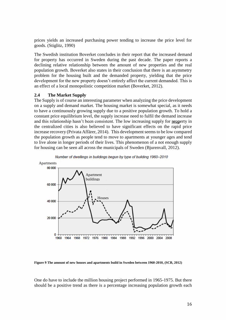
Comparing the Swedish housing market with the market in the United Kingdom, one
can see a pattern that may be applicable in both countries. In the United Kingdom,
house prices increased by over 200 % during the decade prior the financial recession in
2008. During this period, the debt ratio per capita increased by 370% percent (Bank of
England, 2014).
After the financial crisis, the housing prices in the UK dropped. This chain effected
banks to act more carefully and the amount of money lent out dropped by more than 50
percent, resulting in stricter loan regulations making it harder to purchase mortgages.
Economic theory concludes that as people aren’t able to lend as much as before, they
are not able to pay as much as before, yielding the invisible hand to move the price
index for the housing market in UK proportionally equal to the drop in the lending per
capita (Smith, 1759 & Bank of England, 2014).
Even though average prices dropped by 11 percent, this did not reflect on the massive
lending drop of 50 %.
Figure 10 The variation in population, Housing Stock, Housing prices and Lending Secured on Dwellings
during 1997-2010 in United Kingdom (Bank of England, 2014)
The missing proportion of the comparison between the drop in prices and the drop in
the lending ration could possibly be explained by other parameters. This thesis will try
to find which variables that also effects house prices and if there is a similar explanation
in Sweden as in the United Kingdom.
2.6 Why and when prices would fall
As previously mentioned, there are discussions about the existence or non-existence of
a Swedish real estate price bubble (Flam, 2014). This term is used to explain the
situation where prices increase rapidly based on beliefs and expectations instead of
rationality and an increased real value. This price increase can’t continue forever,
leading to a burst and a massive drop on the market (Stiglitz, 1990).
As stated previously in this paper, there was a massive price drop on the Swedish
housing market in the 1990s. The effects of this drop where massive in the short run,
18
but the real prices have continued to grow since. This could imply that the 1990’s price
burst wasn’t really a burst for the entire bubble but basically a small puncture of a
continuously growing bubble as it during the 90’s period and in that economic climate
grew too fast. This however doesn’t need to imply that it was the end of the built-up
real estate bubble. As the capital-lending ratio is the highest ever in Sweden, there
might be reason to believe that we might have a bubble steadily growing. To analyze if
the prices are growing in proportionally towards the expected economic changes in the
society, it would be interesting to do an empirical research on this subject. (Lind, 2008)
Basic economic theory states a relationship between price and demand, which is a key
conclusion for many developed theories. If increased interest rates should make it more
expensive to purchase housing, or if the value should decrease according to for example
an increased supply, than these parameters should be significant to the price
development on the Swedish housing market according to the price and demand theory.
This variable does not however have to yield significant effects, as other factors may
be more important on the Swedish housing market than basic economic theory. This
should in that case imply that our investigated market doesn’t’ follow an economical
effective pattern. (Smith, 1759) (Englund, 2011)
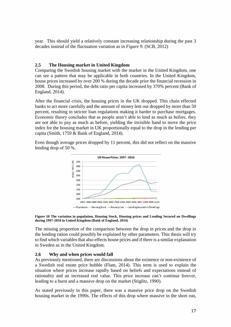
2.7 The interest rate
The central bank uses the interest rate to adjust for macro-economic effects in order to
control and maintain a stable inflation rate. As the economy is affected by recessions
and booms in cycles, the central bank varies the interest rate to keep a consumption
level and price development stable. As the central bank changes their interest rate,
private banks tend to follow, Figure 11. As interest rates fluctuate, Adam Smith’s
economic theory of the invisible hand concludes that since the price of mortgages
varieties over time, the amount of mortgages purchased should fluctuate accordingly.
As mortgages become lower, the price development should decrease. (Smith, 1759)
(Riksbanken, 2014)
Year
Figure 11: The Swedish Central Banks interest rate variation during 2006-2013. (Riksbanken, 2014)
2.8 The lending ratio
Figure 4 describes per capital lending ratio for Scandinavia and Germany during the
21st century’s beginning. However the per capita lending has not followed the same
Apartments
Percentage points
19
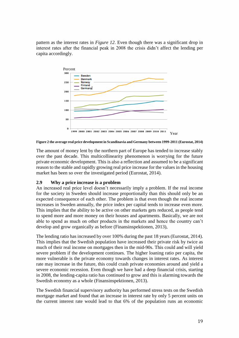
pattern as the interest rates in Figure 12. Even though there was a significant drop in
interest rates after the financial peak in 2008 the crisis didn’t affect the lending per
capita accordingly.
Year
Figure 2 the average real price development in Scandinavia and Germany between 1999-2011 (Eurostat, 2014)
The amount of money lent by the northern part of Europe has tended to increase stably
over the past decade. This multicollinearity phenomenon is worrying for the future
private economic development. This is also a reflection and assumed to be a significant
reason to the stable and rapidly growing real price increase for the values in the housing
market has been so over the investigated period (Eurostat, 2014).
2.9 Why a price increase is a problem
An increased real price level doesn’t necessarily imply a problem. If the real income
for the society in Sweden should increase proportionally than this should only be an
expected consequence of each other. The problem is that even though the real income
increases in Sweden annually, the price index per capital tends to increase even more.
This implies that the ability to be active on other markets gets reduced, as people tend
to spend more and more money on their houses and apartments. Basically, we are not
able to spend as much on other products in the markets and hence the country can’t
develop and grow organically as before (Finansinspektionen, 2013),
The lending ratio has increased by over 100% during the past 18 years (Eurostat, 2014).
This implies that the Swedish population have increased their private risk by twice as
much of their real income on mortgages then in the mid-90s. This could and will yield
severe problem if the development continues. The higher loaning ratio per capita, the
more vulnerable is the private economy towards changes in interest rates. As interest
rate may increase in the future, this could crash private economies around and yield a
severe economic recession. Even though we have had a deep financial crisis, starting
in 2008, the lending-capita ratio has continued to grow and this is alarming towards the
Swedish economy as a whole (Finansinspektionen, 2013).
The Swedish financial supervisory authority has performed stress tests on the Swedish
mortgage market and found that an increase in interest rate by only 5 percent units on
the current interest rate would lead to that 6% of the population runs an economic
Percent
20
deficit. More than 65% of the Swedish population is currently in a state where they are
living in houses that have been bought by 90% loaned money. These numbers are value
adjusted and as property tends to increase in value, the population tend to increase their
loaning from private banks (Finansinspektionen, 2013).
The Swedish financial authority is currently producing an extensive market value
review and the prospect is that they will conclude that the Swedish housing market
value is overvalued by up to 20%. Two important parameters that have affected this
overvalue and which are analyzed are the mortgage-value ratio as well as the lending-
income ratio per households. A reason for which the impact of the real estate crash in
the 1990’s was so severe was due to the high lending-income ratio of 31%. This ratio
has now increased to 46% of the total income. This increased vulnerability comes from
mortgage institutions being able to lend out money at low unfixed interest rates. Should
a crash occur, then these mortgage rates would increase and possibly yield greater
macro-economic effects than the real estate crash in Sweden, 1990
(Finansinspektionen, 2013).
A reason for the housing market getting overpriced may come from speculation and
expectations that prices will always continue to grow. “The great fool theory” explains
the concept of how buyers are ready to pay higher prices for assets than of consumable
goods (Fox, 2001). Even though the buyer knows that the value of the property is lower
right now than what he’s paying, it might not be lower than when he’s selling the asset
in the future. Therefore the market builds up a spiral of increasing values based on that
the markets’ buyers expect the real prices to continue to grow. This concept of “the
greater fool theory” as a phenomenon could actually partly be true on this market, as
the market may not have found the long run real price equilibrium level. There has
been a real price development as shown in Figure 5, since the 1980’s and there may lay
some truth in this expectation. In the end however, the market will sometime get
saturated and real prices won’t continue to grow. If people have purchased housing at
higher prices than this equilibrium price, then as a result of a stagnated market, they
have made a loss. (Segerborg & Ahlgren, 2010)
2.10 The mortgage market
Approximately two thirds of the Swedish population live in houses and apartments
where the mortgage ratio lies higher than 85% of the value for the property
(Finansinspektionen, 2013). The mortgage markets is therefore a significant parameter
for the real price development on the housing market as it defines how much money
that a household can purchase property for. The mortgage market is somewhat
regulated in Sweden and the cost per mortgage may vary depending on income and the
location of the property among others.
To be able to buy a mortgage one needs to set up some ground rules. The Swedish
institution of finance has decided that the mortgage receiver needs to come up with a
cash contribution of 15% of the total mortgage value. The mortgage institution offers
different time periods to fix the interest rates and you also need to sign an amortization
plan for how long you aim to have the money loaned. (Finansinspektionen, 2013)
The housing market is mainly based on loaned money. The interest rates and
amortization requirements are therefore crucial variables that would affect the price
development. These secularities makes the market even more complex and therefore

21
more interesting to investigate to see how different values affect the prices and in the
end how one should think when investing in real estate.
The amount of cash contribution towards mortgages is discussed by the Swedish central
bank. If you increase the capital per lending ratio than that effects the price development
on the market as people have harder times to come up with increased capital. This
regulation can be used in order to cool of a heated housing market (Sveriges Riksbank,
2014).
22
3. Data and variables This part described the variables used to analyze the price development on the Swedish
housing market.
3.1 Price index
Price index is the dependent variable for the thesis. The variable is a measure of the
price development on the Swedish housing market. Valueguard Corporation has
supplied this paper with index values for the price development for all properties sold
each month/3-month/6month in each municipal between the years 2005-2013. The
supplied data also incorporates a dummy-variable for apartments or houses as well as
an average square meter variable. The index value starts with the index base number of
100 for each municipality. The value incorporates the average price index for all
apartments/houses that our sold for each municipal during the observed years. To
perform an annual index we have used a moving average number for each year. The
index value increases in percentage units. This variable is named index in our
regressions (Valueguard, 2014).
3.2 Square meter price
Valueguard Corporation gathered the inflation adjusted average square price for all
housing sold in each municipal at our starting year 2005. The variable is used to adjust
for price changes depending on the size of an apartment. Price and demand correlation
implies a decreasing willingness to pay for larger quantities (in this analyze, more
square meters). This variable is included to adjust the price development depending on
size. The index variable is multiplied by the average square meter price for Sweden
during the observed years. This yields the real price development for housing in each
respective municipality. The variable is transformed, as a percentage price increase
doesn’t reveal the real price change.
For investors in houses and apartments, the percentage increase is the most interesting
variable but to analyze the effects of other parameters and the real price development
as a whole, this variable need to be incorporated. Some municipals starts with lower
starting prices than others, the square meter price is significant to find the real price
development. The variable is named sqmp in our regressions (Valueguard, 2014).
3.3 Population
The central bank of Sweden concludes that a reason for increasing housing prices is
increased population (Flam, 2014). The population development is assumed to have
significant impact on the housing prices. As the market increases, the demand for a
fixed good tends to increase, yielding higher prices. In this case, population is defined
in tens of thousands. The variable is supplied by SCB, the central agency for statistics
in Sweden. The variable is named pop1 in our regressions (SCB population, 2014).
3.4 New houses
The price and demand correlation concludes that with larger available quantities, prices
tend to go down. In this empirical analyze, the quantity is housing which make the
supply of new houses a relevant variable to include in the model. New houses are a
variable used in this model to incorporate the increased supply for apartments and
houses within the model. An increase in houses is regarded as an increase in quantity

23
and is therefore regarded as having a negative effect on the housing price development.
(Schiller, 2007)
The variable is defined as finished houses for sale. This variable had not been
calculated for 2013, which meant that we generated the value for 2013, by a moving
average. The value is supplied by SCB. The New houses variable is named nhouse in
hour regressions (SCB new houses, 2014).
3.5 New companies
The amount of new companies is assumed to have a significant effect on the price value
index as Jane Black shows these affects in 1996. As new companies emerge, this often
yields new employment opportunities, which increases the demand for housing,
resulting in an price increase for this municipal (Black, 1996).
The Swedish institution samples the amount of new companies created for corporations.
The variable is defined in amounts of companies started. The variable is named ncomp
in our regressions (Bolagsverket, 2014).
3.5 Foreign background
The amount of people coming from a foreign background is assumed to have a
significant effect on the price index variable as shown by Albert Saiz in 2007. Saiz
shows a positive correlation between an increases of immigrants ante the development
in housing prices in the US (Saiz, 2007).
The foreign background is later used as an instrument for the population growth
variable. This variable could partly explains the population gross in a municipally and
is therefore used as an instrument variable for population grows. The variable is
supplied by SCB and defined in per cent units, which was multiplied by the population
variable and transformed into real amount of people. The variable is named fback1 in
our regressions. (SCB population, 2014)
3.6 Foreign born
The same assumptions are drawn as for the variable foreign background (Saiz, 2007).
The differences are that in the foreign background variable, one could be included when
being born in Sweden by parents born in another country. This variable could partly
explains the population gross in a municipally and is therefore used as an instrument
variable for population grows. The foreign born variable captures only the population
born outside of Sweden. The values are supplied by SCB and measured in per cent units
and transformed into amount of people by multiplying by the population variable. The
variable is named fborn1 in our regressions. (SCB population, 2014)
3.7 Unemployment rate
The unemployment rate for a certain municipality is assumed to yield negative effects
on the average price index as when your unemployed you tend to have a low income
yielding a low purchase of power (Black, 1996).
This variable is defined as people registries as unemployed by the institution for
unemployment. The variable is defined by the amount of people unemployed. The
variable is named u in our regressions. (Arbetsförmedlingen, 2014)

24
3.8 Amount of break-ins
The amount of break-ins variable is used as a measurement for how safe a certain
municipal is. Robert T. Greenbaum derives that there is a negative correlation between
crimes and the housing price development which could imply significant negative
effects on the price index value. Greenbaum shows that the effects of crimes are larger
depending on the average wealth-level within a district (Greenbaum, 2006).
The amount of break-ins is defined by its natural value and supplied by the Swedish
national council for crime prevention, BRÅ. The variable is named burg in our
regressions. (BRÅ, 2014)
3.9 Total amount of crimes
The total amount of crimes variable is incorporated in the model by the same reasoning
as the break-in variable. It is assumed to be a variable that incorporates the safety-level
of a municipal and an increase in crimes tends to decrease the development rate for
housing (Greenbaum, 2006).
The variable is defined by its natural number and supplied by the national council for
crime prevention, BRÅ. The variable is named crimes in our regression. (BRÅ, 2014)
3.10 Amount of jobs available
The amount of jobs available variable is included in the model as people might move
between municipals if there is a possibility of getting a job in that municipal. The
increase in job availability could increase the population leading to an increased
demand and a higher price index (Black, 1996).
The variable is given by its natural number and supplied by the institution of
unemployment. The variable is named jobs in our regressions. (Arbetsförmedlingen,
2014)
3.11 The interest rate
The central banks interest rate is assumed to effect the price index variable negatively
as an increased interest rates leads to that private banks increase their interest rate and
the price for mortgages more expensive leading to an assumed decrease in the price
index variable. The effects of the interest rate has however varied over time, showing a
positive relation between increased rates and housing prices prior to 1970’s in the US.
The correlation between increased interest rates and housing prices has been negative.
The prior positive correlation is assumed to occur due to external factors (Harris, 1989).
The variable is supplied by the central bank of Sweden and is defined in percent units.
The variable is named repo in our regressions. (Ekonomifakta, 2014)
3.12 Average Income-level
The average disposable income level for the municipality is included as an increase in
income yields a higher purchasing power and this is assumed to increase the price index
variable. Increased average mortgage payments can also be captured by disposable
income level. The relationship between income level and housing prices is positive,
implying that an increased level of income for a district will yield an average increase
in house prices for this district (Brown, 1980)

25
This variable of income is inflation-adjusted and supplied by the institution for statistics
in Sweden, SCB. The variable is named income in the regressions. (SCB Income, 2014)
3.13 GDP
The GDP level incorporates in what stage of the market a country currently is and this
might affect the development of the price index variable. Increases in the GDP-level
per country will yields an increased aggregate demand of houses and housing price has
a positive shocks (Iacoviello, 2005).
This GDP-value is index adjusted with the starting value of 100 at year 2005 and
supplied by the central bank of Sweden. The variable is named bnp in our regressions.
(Sveriges Riksbank, 2014)
3.14 Fokus ranking
To try and incorporate as many external factors as possible this paper includes a ranking
parameter that has been set by the Focus time script. The Fokus ranking variable is an
instrument variable based on the Swedish time script Fokus ranking of the best
municipals to live in based on 30 parameters. The parameters for which Focus bases
their ranking systems are shown in Appendix 1. The municipals with the most suitable
value receive ranking 1 and the least suitable receives ranking number 290. (Fokus,
2014)
The variable captures values for education quality, elderly care, and the business
environment. The variable includes qualitative values of in what extent the population
like their municipal and so on. These values are difficult to capture individually and has
therefore been used by Fokus through market surveys and compiled into this ranking
system. The Fokus magazine releases this information annually to decide which are the
best municipals to live in Sweden and this paper attempts to explain the effects of their
results on the real price development. Each incorporated variable is shortly defined in
Appendix 1 (Fokus, 2014).
26
4. Method This chapter of methods incorporates the empirical structure prior to the analysis. The
data set and variables are described as well as our different empirical estimation
models. The chapter also incorporates the limitations and divisions used in the
empirical models. The author also discloses his initial beliefs and expectation for the
estimation.
The empirical dataset used is a dynamic panel dataset. The panel dataset enables the
author to view the development over time. Having the dataset dynamic makes the
development adjust towards differences in for example real income levels for each
municipality. To analyze this data, the author has chosen the Xtabond2-model.
The simplest form of an empirical panel regression to find a significant relationship
between prices and parameters on a panel data set is to estimate a standard generalized
least square straight-line estimation. The more complex and the more variables
affecting the model, the more complex becomes the empirical models. (Trivedi, 2010)
There are requirements that need to be fulfilled in order for the models to be acceptable.
Homoscedasticity is a Gauss-Markov requirement, meaning that the error terms need
to have an expected value of 0 and a constant variance. To be able to analyze our
econometric models and deal with a possible hetroscedacity, the robust command is
included for the estimations in STATA. The error terms need to follow a normal
distribution, which is controlled for by analyzing the Jarque-Berra test in Table 7.
Endogeneity is a problem for most estimation models as parameters may affect an
explanatory variable in some ways without affecting the investigated variable directly.
To deal with some endogeneity, we analyze the Hausman test and later develop our
estimations by including instrumented variables.
4.1 Limitations for the model
Missing values for 62 municipalities’ yields that there are 228 municipals consisting of
houses and apartments in Sweden in our panel dataset. The reason for which not all 290
municipalities are included is due to incomplete data for price development through the
investigated period. We start of by adjusting the included municipalities as observations
in a panel study for 9 years, 2005-2013.
Since the dataset is under a short period of time, this might have some effect on the
creditability for our results. During the investigated period there has been a financial
crisis, which possibly have affected many of the macro economic variables in other
ways than normally. The dataset basically starts of by reaching the top of a state of the
market peek and has had a declining correlation since. This negative effect could impact
on the estimations.
Multicollinearity is a problem that we are dealing with constantly in estimating
econometric models. Having the amount of jobs and unemployed in the same models
may affect each other within the model. The same argument can be derived for the
foreign people and foreign background variables (Table 2, Model II).
We conclude that an estimated regressor is significant at a 5% significance level.

27
4.2 Division
As Flam described in the article from 2014, a share of why housing increases could be
that people are moving in to larger cities (Flam, 3014). To analyze if this conclusion by
the Swedish central bank is relevant, or if there are any differences between municipally
sizes, the dataset is divided into 3 groups. The observations are divided into three
different groups’ small, medium and large municipals. Small municipals are defined as
smastad and include municipals with a starting population of less than 20 thousand
inhabitants, yielding 123 municipalities. Large municipals are the 22 municipalities
having a population greater than 70 thousand and called “storstad”. Medium sized
municipals are the 83 in-between referred to as “medelstad” in our results.
4.3 Models
4.3.1 Xtabond2-model
There are different methods for analyzing the relationship between the real price
increase affects by the “quality of living” variable. Since this dataset includes a large
sample of observations during a relatively short period of time. This paper uses the
Arello-Bond Xtabond2-model.
The Xtabond2-model is a developed model based on a difference and systemized
generalized method of moment’s model, GMM. The model is developed to yield
regressions and estimations on dynamic panel estimators based on cross sectional time
series data. (Roodman, 2009)
The model is able to fit two closely related dynamic panel-data model. The first is the
Arello-Bond model from 1991. The difference from the Arello-Bond model is that the
Xtabond2-model uses a two-step standard error correction, which will be described
later on. The Arello-bond model is sometimes referred to as the difference GMM model
while this second, augmented version is refer to as the system GMM-model.
The model estimators are designed for a dynamic small time period dataset with a large
population size that may or may not contain fixed effects. This model separate from
these fixed effects, idiosyncratic errors that are heteroscedastic and correlated within
but not across observed individuals.
Equation 1
The independent variable in the model, xit, is a vector of strictly exogenous covariates
that are ones dependent on neither of the current nor by past error terms. The wit
variable is a vector of predetermined covariates, all of which may include a lagging
effect on our dependent variable Yit. Endogenous variables and covariates are all of
which somewhat correlated with the part error term vi. Vi is a term that captures the
individual effects and how these are potentially correlated with previous and current
error terms.
The model uses a first-differentiation to remove the captured vi and hence eliminate
potential sources of omitted variable bias in out estimations. Differencing the variables
that are predetermined but doesn’t need to be strictly exogenous makes them
endogenous in the model.

28
The model is a combined development of the Holtz-Eakin, Rosen and New model from
1988 as well as the Arello-Bond model from 1991. These GMM-model estimators state
that instruments in the differenced variables are not strictly exogenous as of their
abilities to capture lagged effects. This differs from strictly exogenous instruments were
they’re assumed to be strictly uncorrelated with no past or current errors.
The original Arello-Bond model contained a problem with lagged levels of poor
instruments when applying the first-differentiation. If the variables acted according to
a random walk, meaning that they were impossible to forecast. The original equations
can be added as instrumented lagged levels within the model to increase the models
efficiency. In the Xtabond2-model, variables are instrumented with a suitable amount
of lagged periods that is best applicable for the model. To be able to perform these
transformations, one has to assume that the differences between municipals in this case
are uncorrelated unobserved fixed effects. The xtabond2 model implements both first
difference estimators as well as orthogonal estimations.
Another development in the Xtabond2 version is the introduction of the Mata version
that includes orthogonal deviation transformations instead of taking the first difference
as before. The difference is that the orthogonal deviation transformation subtracts the
previous average of an observation instead of subtracting the first difference. This
smoothens out forecasts and also removes the fixed effects within the model. As lagged
observed variables don’t enter the transformed model, they continue to stay orthogonal
to the transformed error terms, implying that there shouldn’t be any serial correlation
for the instruments.
Taking the orthogonal transformation instead of first differentiating doesn’t affect the
amount of reduced time periods for the model. For instrumented variables, w, wi(t-1),
are transformed as observations at time period t for individual i. In the Xtabond2, we
apply this for two time lags.
Generalized method-of-moment, GMM estimations need balanced panel sets to
perform a two time lag generally generate numerically identical coefficient estimations
meaning that the instrument set are kept fixed. The orthogonal deviation structure
however, able you to keep a larger sample size including missing values. The reason
for this is the orthogonal transformation, which generates the average change from the
previous observation for your missing value. This makes the model able to work with
larger incomplete data sets while the previous first differentiation models had to drop
these observations.
The xtabond2 model is also an instrumented regression model, making it possible to
include correlated parameters effects on variables that are believed to yield significant
effects on our dependent variable.
The Arello-Bond estimation model deals with time-invariant county characteristics,
fixed effects. These effects could be correlated to the explanatory variables in our
model. The fixed effects are reflected in the error terms for the estimation and are due
to unobserved parameters that affect our dependent variable. (Roodman, 2009)

29
4.3.2 Correlation
In econometric models there is nearly always a problem of endogeneity, meaning that
explanatory variables are affecting each other within an estimated model. To remove
this unwanted effect one can use one of these variables as an instrument when building
an econometric model. To see which variables are correlated with each other, one
performs a correlation matrix in STATA (Baltagi, 2008).
The Pearson’s product-moment correlation coefficient is used for each observation to
calculate the casual relationship within our model.
The correlation value lies between -1 and 1 where the extreme values imply highly
correlation and as the value moves towards 0 implies uncorrelated variables.
The correlation matrix is used in the model to see how variables develop according to
other variables. If there is a high correlation between variables, than they act similar to
each other.
4.3.3 Fixed and random effect
In a panel regression dataset when sampling observations under a specific time period
there usually is a staring difference between the observations. These differences are
used in terms of random or fixed effects. The term is used to describe differences in our
intercept and development between individuals, municipals in our case. (Baltagi, 2008)
The fixed effect concept states that the differences between observations is caught by
the intercept and is constant over time. Taking the first difference of such a model
deletes the problem of fixed effects.
A random effect model states that the differences between municipalities in our case
are random over time. The random effect concept tells us that there is some unobserved
difference between municipals that affects the observations differently.
To find which model is best suitable to estimate Durbin, Wu and Hausman developed
the Hausman test. The Hausman test is a chi2-test that of two estimated models error
terms. The Hausman test can test for endogeneity and also if there if a random or fixed
effect model is more suitable when estimating our regressor’s for a panel data set. When
testing for random or fixed effect models, the null hypothesis is that there is a random
effect within the model. (Greene, 2008)
4.5 Empirical expectations
My expectations of the empirical estimations are that the price variable will be
negatively affected by an increased interest rate. Interest rates yield more expensive
mortgages and, hence a reduced property budget yielding decreased prices.
The population growth affects the demand function, as more people desire a fixed
supply of housing yielding increased prices. Immigration from people from other
countries or people with a foreign background can however yield negative effects on
the price development. The reasoning behind this expectation is that people coming
fleeing from other countries has a lower average income reflecting in a multi collinear
effect of having a negative effect.
30
Increased lagged income should reflect positively on the price development as people
basically afford to spend more on housing. The amount of jobs and companies started
should yield an attraction from unemployed, yielding an increased demand and higher
prices. An estimation parameter for unemployed however is believed to effect the price
development negatively.
The amount of burglaries and crimes in a society is expected to yield negative effects
on the prices, as people want to leave in safe places where you don’t get robbed, at least
I do.
Lagged GDP levels should also reflect positively as an increased GDP level tends to
increase the standard of living and the real income, yielding increased price levels.
Systematically lagging the dependent variable is something that the author believes will
have a positive sign to explain the phenomena of the exponential price development.
The parameter estimation for the perceived “quality of living” variable will probably
gender a negative sign. Having a good quality of living in a municipally yields a low
value for the Fokus variable.

31
5. Results
This chapter captures the empirical results from the estimated models. The regression
results referred to in text form and showed in Appendix 2.
5.1 The Hausman test
Table 1, Model I&II are results from two generalized least square regressions with
adjustments for random respectively fixed effects. Table 2, Model I is the results of a
Hausman test that concludes that the observations seem to include a fixed effect
difference.
5.2 The Xtabond2 model
The results from the Arello-Bond Xtabond2 models are shown in Tables 5, 6.
From the results in Table 5. Model III we read that the population growth and the Fokus
ranking variable are the only significant variables that effect the index variation. Both
affect the dependent variable negatively.
The population growth and the focus ranking variables have significant effects on the
square meter price development.

32
6. Analysis This chapter analyze the results from chapter 4, interpreting the results and comparing
them against economic theories. The author also includes some personal opinions from
the results.
6.1 The Arello-Bond model
The reduced Arello-Bond Xtabond2 model, Table 6, Model I shows that there are a
negative correlation between the Fokus Ranking variable and the real house price
development. The model also yields a significant positive relationship between
population growth and the previous price development on the market. After eliminating
insignificant parameters to the Xtabond2-model, the derived model can be shown as
Equation 2.
Equation 2
We are analyzing a short time period of observations with a significant fixed effect
within our sample. This sets up the right conditions for applying the orthogonal
deviating Xtabond2 model. The results from this Xtabond2 model yields that the Fokus
ranking has a significant effect on the price development for the municipals in Sweden.
Having a well-respected education, quality elderly care and a healthy environment in
the municipals yields low values for the Fokus ranking. Increased Fokus ranking values
significantly inhibits the price index to grow, Table 6, Model I. The population growth
and interest rate also effect the index development negatively Table 5, Model II & Table
6, Model I.
Table 6, Model I also shows that the population growth increases the price per square
meter, which seems reasonable as the demand increases and the estimated parameter
for the “quality of living” variable is negative which is consistent towards economic
theory.
33
7. Discussion The real price increase of property leads to that the population in Sweden are less able
to purchase other goods than in a stable market. Looking at the development for housing
prices over the past years, one can easily see that it has been growing exponentially.
This has led to a psychological effect property is always a good investment. And it truly
seems to be, even the deep crash in the real estate market in Sweden during the 1990s
only took 7 years to recover from, and to be in the same real price level as. In fact,
prices have grown by 250% since the recovery in 1997. This implies that there is no
really short-term reason for why the real estate markets price development should
stagnate. It should therefore be regarded as an attractive but ineffective economic
market for investments. Even though adjustments in variables as interest rate, the GDP-
level income level and unemployment level might push down prices significantly, this
doesn’t reflect the price changes in the market.
The main belief that, the price development was centralized towards the largest
municipalities showed to be completely inaccurate. Instead, the advice for investment
possibilities towards real estate agents and mortgage institutions would be to invest in
municipals as Mjölby, Motala and Hudiksvall where the return on equity has increased
by nearly 500% during the past 8 years. (Valueguard, 2014)
For the Swedish society the increased lending ratio and the increase income spent on
housing is both a short and long term threat. History tells us that even though the real
values for housing continues to increase, there have been a couple of speed bumps on
the way. As the debt ratio has increased even more than the development prior the 1990s
real estate crisis, this is truly worrying. As I discussed previously in this paper, 1990s
crash wasn’t really a case of a bubble bursting but merely a ventilation release for a
bubble growing too fast.
The empirical evidence gathered by the statistical institution agency in Sweden clearly
shows us that the price and lending increase has sprung up to the 1990s rate and past.
Off course other parameters than the price development and lending similarity affected
that there was a crash in the 1990s, Figure 8. The central banks unconsidered move of
a shock increased interest rate was a major factor and something that the Swedish
monetary agencies have learned from, probably. There is however other similarities as
both situations came of another economic crisis.
The economic problem for Sweden is not only if there is a bubble about to burst or not,
the problem is that the Swedish population are lending more money than they are able
to pay back based on a phenomenon that real housing prices will continue to grow. This
statement can’t occur. Even though the Swedish population has had a real income
increase for many years, the lending and property prices are growing faster leading the
proportions of how much capital spent on housing to shift. There must come a breakage
point where the market is stagnating as people can’t spend all of their money on
housing, other factors are clearly significant as well. Therefore, weather the stagnation
will come in 1 year, 5 years or 50 years doesn’t matter. When the stagnation occurs, the
Swedish society will have a debt ratio that can’t be paid back to the private banks. This
could lead to a domino effect where the Swedish society collapses. However, my
personal belief is that reality doesn’t need to be as dark as I just formulated. There are
adjustments that can be made that could stabilize this market.
34
Amortization requirements. This adjustment is currently in the making by the large
private banks in Sweden. The amortizing rate has increased to 57% percent of the
mortgage population. This is an increase of 47% since 2011 and this increase is a
necessary requirement to stabilize this price development (Finansinspektionen, 2013).
However, the average amortizing ratio is still on 148 years. Implying that customers
are basically able to borrow money without having a realistic way of paying them back.
This phenomenon has occurred based on that the property value always will continue
to grow. Increasing and shortening the length of a mortgage able people to afford lower
loans as their monthly income takes a harder hit by the amortization requirement. This
could cool down the economic climate on the market without having a market failure.
The problem is that market doesn’t only move according to economic adjustment, it
moves also according to expectations. If the population of Sweden believes that the
monthly costs for housing will increase, than the market value will decrease then we
have only pushed the crash forward. I believe that a crash is inevitable, as the income-
lending ratio can’t continue. It could therefore be smart to push the hit towards us no
before the lending ratio increases even further. This would stop the price development
and the market could stagnate.
A problem with increasing the amortization requirements is that people could seek
mortgages from other countries, leading to that the Swedish monetary capital gets
pushed overseas. It could also mean that the property would only be bought by people
having old money or by foreign money. This doesn’t necessarily mean a bad thing.
7.1 Why suppliers doesn’t produce more housing
The amount of new houses and apartments didn’t yield significant effects in our
regression but we still believe that the parameter is important. The supply and demand
relationship is a cornerstone in economic theory and it would be highly surprisingly if
the supply didn’t affect the demand. The problem is probably that the variation in newly
produced property doesn’t vary enough within municipals. A reason for this is a highly
regulated market that makes it difficult for the construction companies to fulfil the
demand. If this market should be more open and deregulated then perhaps more
apartments could be built. Look at Stockholm city for example, we find highly priced
apartments and a high demand. This should attract construction companies to exploit
the city. However, regulations are such that the capital city design shouldn’t be changed
as much. Construction companies are not able to build higher houses that could contain
more apartments due to these regulations. This increases the risk for construction
companies, as people are demanding apartments in the central part of town and not
outside where they are able to build them. Should the market deregulate this than we
would probably see significant effects on the amount of houses produced. (Villaägarna,
2013), (Boverket, 2012)
7.2 Fokus ranking
The focus ranking parameter has shown significant effects on the price development in
straight-line GLS, Instrumented GMM, and autoregressive regression estimation. This
effect states that soft society values have important effects on the housing market.
People incorporate qualitative parameter into their valuation and this effects the price
development.

35
8. Conclusion and suggestions Empirical results show that the Swedish society in general is spending more and more
of their net income on housing costs. Historical so-called real estate crashes have led to
short time price drops but the market continues to recover and keep growing in real
prices.
Systematically including lagged parameters for the dependent variable result in a
significant positive estimation regressor. This estimator includes some of the
phenomena of prices tending to increase, as they’ve always tended to increase.
Including the instrumented Fokus ranking variable shows significant parameters, which
incorporates some of the complexity on the market. The real estate market can’t be
analyzed as a simple goods market since there are many alternative costs effecting why
the prices tend to increase. Purchasing real estate in a trending, upwards moving
municipal on the Fokus ranking will increase the value of the property in the future,
making the purchase an investment asset. The Fokus and the lagging dependent
variable capture some of the unknown effects of such as quality of living and future
prospects. Having the significant effect of a positive effect by the lagged changes
explains some of the psychological effects on the price and index variation. The
Swedish financial supervisory authority states that this psychological change might
have made the housing market to become overvalued by up to 20%.
A GLS estimation of the differences between municipal sizes concludes that smaller
municipals are affected by amount of people with a foreign background, new
companies entering the municipal, and interest rate changes. Increasing the local
foreign background population or interest rate decreases the real housing prices whilst
a company entering yields a positive effect on the price level. Prices in medium and
large municipals are significantly affected by the interest rates negatively and GDP
level positively. Their empirical significance concluded that investors in real estate
should Fokus their investments within the low 25-50% population municipals in order
to generate the highest percentage increase of their real estate investments.
The Arello-Bond Xtabond2 model removes the fixed and endogenous problems reduce
the model to being significantly affected by the Fokus ranking system, interest rates
and the population growth. This model is believed to be the most suitable model to
analyze the Swedish housing market as it mixes the advantages shown by the other
three estimations. This yields that to effect the price development, the government
should temper with the population growth, the “quality of living” variable and the
interest rate. The Fokus ranking system and the population growth is very complex to
deal with but the interest rate however is directly set by the central government. Setting
a higher interest rate today could reduce the lending development and cool of the market
in the short run.
The real price increase development enables to private consumption to spend relatively
less of their income on other consumption goods. If this phenomenon would continue,
the real consumption level would have to decline. This would affect the Swedish GDP
development and is therefore a problem that has to be dealt with by the Swedish
government. Increasing the costs for mortgages would generate a price drop or
stabilization, as people aren’t able to borrow as much money. This would reduce the
market risk for future interest rate changes cooling down an exponentially price
36
growing market. The mortgage cost structure should then slowly be moved towards a
bit lower interest rates at higher amortizing rates, keeping the cost for mortgages higher
than the current whilst stagnating the price development.
The real price development on the market will stagnate sometime in the future as real
prices can’t reach total real income. If the society are lending money for overvalued
estates, than a stagnation will yield into a deep recession as nearly 2 thirds of the market
population would have assets that are lower than their lend money.
Neither of the empirical result concludes that the supply of new housing property
effects the price development, which is quite contradictory towards the price and
demand theory. The reason for this unexpected insignificance believes to be the
constant variation for the variable. Here lies the actual problem according to me. If
there would be an unsaturated supply for housing, than prices wouldn’t continue to
increase as much. The government should therefore deregulate this market so that
construction companies can fulfil the market demand.
The results of the derived model shows that increased quality of living within a
municipality compared to other municipalities in Sweden yields an increased price
development compared to these municipalities. This implies that you can find a
possibility of investing in municipalities that are increasing in ranking of the quality of
living by Fokus magazine to increase the expected rate of return of your investment in
the housing market.
8.1 Future research
Investigating the social and economic effects of the million housing programs effects
on the Swedish society would be an interesting subject. We see rapports of increased
segregation in our society. As more immigrants and refugees seem to move into these
project districts, it would be interesting to see how the increased segregation in Sweden
has been effected.
Investigation if there is any causal correlation between the foreign backgrounds
parameters’ effects on the price development compared to the increasing support of
xenophobic political party “Sverigedemokraterna” would be interesting to investigate.
37
9. Reference Andersson 2014, Klas Andersson, “Störst drag på villapriserna”, SvD Näringsliv.
http://www.svd.se/naringsliv/pengar/storst-drag-pa-villapriserna_8991076.svd, 2014-
06-02
Angser & Åkerwall, 2011, Angser, Emma & Åkerwall, Hanna, “Bostadsbubblan,
Köparnas förväntningar vid bostadsköp”, KTH, 2011
Arbetsförmedlingen, 2014, Tidigare statistik, http://www.arbetsformedlingen.se/Om-
oss/Statistik-prognoser/Tidigare-statistik.html, 2014-06-02
Bank of England, 2014, Statistical Database and Nationwide House Price Survey,
“WHY ARE HOUSE PRICES SO HIGH?”
http://www.positivemoney.org/issues/house-prices/, 2014-06-02
Bank of England, 2004, “Asset pricing and the housing market”, Olaf Weeken, Bank’s
Monetary instruments and Market division.
Baltagi, 2008, Baltagi, Badi H., Econometrics, p. 221-234, Syracuse University,
Central for Policy Research, USA, 2008
Birch Sorensen, Peter, “The Swedish housing market: Trends and risks”, University of
Copenhagen, Rapport till Finanspolitiska rådet 2013/5, 2013.
Bjurenvall, 2012, Bjurenvall Thomas, “Bostadsbyggandet lågt under lång tid”,
http://www.scb.se/sv_/Hitta-statistik/Artiklar/Bostadsbyggandet-lagt-under-lang-tid/,
2014-06-02.
Black, Jane, de Meza, David & jeffreys, David, 1996, The Economic Journal, “House
Prices, The Supply of Colleteral and the Enterprice Economy”, Vol 106, No 434, pp.
60-75.
Bolagsverket, 2014, Statistik om företag och föreningar,
http://www.bolagsverket.se/om/oss/etjanster/statistik/statistik-1.3538, 2014-06-02.
Boverket, 2012, “Bostadsmarknaden 2011-2012, Vad händer på bostadsmarknaden,
Med slutsatser från bostadsmarknadsenkäten 2011”,
http://www.boverket.se/Global/Webbokhandel/Dokument/2011/BME-2011-2012.pdf,
2014-06-02
Brown, 1980, James & Li, Mingche M., “Micro-Neighborhood Externalities and
Hedonic Housing Prices”, Land Economics, Vol. 56, No. 2, 1980, University of
Wisconsin.
Bruss, 1986, Bruss, Robert J, “Greater FoolThery Can Lead To Expensive Home
Investment”, Chicago Tribune.
BRÅ 2014, Brottsförebyggande rådet, http://statistik.bra.se/solwebb/action/index,
2014-06-02

38
Ekonomifakta, 2014, “Reporäntan”,
http://www.ekonomifakta.se/sv/Fakta/Ekonomi/Finansiell-
utveckling/Styrrantan/?from1554=2005&to1554=2014, 2014-06-02
Englund, 2011, Englund, Peter, Sveriges Riksbank, “ Swedish house prices in an
international perspective”,
http://www.riksbank.se/Upload/Rapporter/2011/RUTH/RUTH_chapter1.pdf, 2014-
06-02
Eurostat, 2014, Statistiska Centralbyrån, SCB, “Hushållens skulder på hög nivå”,
http://www.scb.se/sv_/Hitta-statistik/Artiklar/Hushallens-skulder-pa-en-hog-niva/,
2014-06-02
Ezzet-Lofstom, Roxanne, 2004, University of Texas at Dallas, “Valuation of
Metropolitan Quality of Life in Wages and Rents”,
http://www.huduser.gov/portal/periodicals/cityscpe/vol7num1/ch2.pdf, 2016-01-05
Finansinspektionen, 2013, “Den svenska bolånemarknaden 2013”,
http://www.fi.se/upload/43_Utredningar/20_Rapporter/2013/bolan_2013_2.pdf,
2014-06-02.
Flam, Harry, “Finns det en prisbubbla på bostadsmarknaden”.
http://ekonomistas.se/2014/01/14/finns-det-en-prisbubbla-pa-bostadsmarknaden/,
2014-01-14
Fokus, 2014, “HÄR ÄR DET BÄST ATT BO”, http://www.fokus.se/fokus-rankar/, 2014-
06-02
Folkesson & Petterson, 2011, Folkesson, Jakob & Pettersson, Viktor, “Är ett kraftigt
prisfall på bostadsmarknaden I Stockholmsregionen rimligt I framtiden, KTH, 2011
Fox, Justin, 2001, “When Bubbles Burst Tulips. Dot-coms. Hey, manias happen. But
most don't lead to economic disaster”,
http://archive.fortune.com/magazines/fortune/fortune_archive/2001/06/11/304604/ind
ex.htm, 2016-01-09
Greenbaum, Robert T, 2006, Tita, George E. & Petras, Tricia L., ”Crime and
Residential Choice: A Neighborhood Level Analysis of the Impact on Housing
Prices”, Journal of Quantitative Criminology, 2006.
Greene, 2008, William, Econometric Analysis, Pearson, 6th edition, 2008.
Harris, 1989, Jack C., “The Effect of Real Rates of Interest on Housing Prices”,
Journal of Real Estate Finance and Economics, “: 47-60, 1989.
Iacoviello, 2005, Matteo, “Housing Prices, Borrowing Constraints, and Monetary
Policy in the Business Cycle”, The American Economic Review, Vol. 95, No.3, pp. 739-
764, 2005.
Krugman & Wells, 2009, Krugman, Paul & Ells, Robin, Princeton University,
Microeconomics, Second Edition, 2009m p. 8, Worth Publishers, 2009.

39
Keynes, 1936, Keynes, John, “The General Theory of Employment, Interest and
Money, p. 313-331, Palgrave Macmillan, 1936.
Lind, H., 2008, “Price Bubbles on the Housing Market: Concept, theory and indicators,
Publication n. 58, The Royal Institute of Technology, Stockholm, 2008.
Nationalencyklopedin, 2014, “miljonprogrammet”,
http://www.ne.se/miljonprogrammet, 2014-06-02
Pearl, 200, Pearl, Judea, “Causality: Models, Reasoning, and Inference”, Cambridge
University Press, 2000.
Porter, 2000, Porter, Michael E., “Location, Competition, and Economic
Development: Local Clusters in a Global Economy”, Harvard Business school,
Economic Development Quarterly, vol. 14, no.1, p. 15-34, feb. 2000
Privata Affärer, 2014, Riksbanken tror på högre bostadspriser, Riksbanken,
http://www.privataaffarer.se/bostad/rb-bopriser-vantas-fortsatta-stiga-under-
prognosperiod-ppu--630460, 2014-06-02
Riksbanken, 2014, http://www.scb.se/sv_/Hitta-statistik/Artiklar/Hushallens-skulder-
pa-en-hog-niva/, 2014-06-02
Roodman, 2009, Roodman, David, “How to do xtabond2: An introduction to difference
and system GMM in Stata, Central for Global Development, Washington, DC, USA,
2009.
Roth & Oke, 1989, Roth, M & Oke, T.R. “Satelite-derived urban heat islands from three
coastal cities and the utilization of such data in urban climatology, University of British
Colombia, Vancuver, Canada, Vol 10, 1989.
Saiz, Albert, 2007, “Immigration and the Housing Rents in American cities”, Federal
Reserve Bank of Philadelphia.
SCB, 2011, Statistiska Centralbyrån, Positiv fastighetsprisutveckling,
http://ninalundstrom.wordpress.com/2013/09/27/positiv-fastighetsprisutveckling-pa-
hyresratter/, 2014-06-02
SCB, 2012, Statistiska Centralbyrån, “Bostadsbyggandet lågt under lång tid”,
http://www.scb.se/sv_/Hitta-statistik/Artiklar/Bostadsbyggandet-lagt-under-lang-tid/,
2014-06-02
SCB income, 2014, Statistiska Centralbyrån, http://www.scb.se/sv_/Hitta-
statistik/Statistik-efter-amne/Hushallens-ekonomi/Inkomster-och-
inkomstfordelning/Inkomster-och-skatter/Aktuell-
pong/302201/Inkomster/LanKommun/303220/, 2014-06-02
SCB new houses, 2014, Statistiska Centralbyrån, http://www.scb.se/sv_/Hitta-
statistik/Statistik-efter-amne/Boende-byggande-och-bebyggelse/Bostadsbyggande-
och-ombyggnad/Nybyggnad-av-bostader/#c_undefined, 2016-02-02

40
SCB Population, 2014, Statistiska Centralbyrån, http://www.scb.se/sv_/Hitta-
statistik/Statistik-efter-amne/Befolkning/Befolkningens-
sammansattning/Befolkningsstatistik/25788/25795/, 2014-06-02
Segerborg & Ahlgren, 2010, Gustaf Segerborg & Max Ahlgren, Landic property
Group, Stockholm, 2010.
Shiller, Robert J., 2007 “Understanding Recent Trends in House Prices and Home
Ownership”, Yale University, http://www.nber.org/papers/w13553.pdf, 2015-01-24
Smith, 1759, Adam, “The theory of moral sentiments”
Sorensen, 2013, Sorensen, Peter B. “The Swedish Housing market: Trends and risks”,
University of Copenhagen, Finanspolitiska rådet
Stiglitz, 1990, Stiglitz, Joseph, “Symposium on Bubbles. The Journal of Economic
Perspectives. 2, 1990, Vol.4, 2, s. 13.
Stiglitz, 2012, Stiglitz Joseph E., “The price of inequality”, 414 pp. W. W. Norton &
Company.
Sveriges Riksbank, 2014, “Aktuell prognos för reporänta, inflation och BNP”,
http://www.riksbank.se/sv/Penningpolitik/Prognoser-och-rantebeslut/Aktuell-
prognos-for-reporanta-inflation-och-BNP/, 2014-06-02
Sveriges Riksbank, 2014,” Riksbanken angriper ränteavdragen”,
http://www.svd.se/naringsliv/riksbanken-angriper-ranteavdragen_8948176.svd, 2014-
06-02
Trivedi, 2010, Cameron, A.A., Trivedi, P.K. Mikroeconometrics Using Sata, revised
Edition, Stata Press
Valueguard 2014, Valueguard AB supplied data of the price index development of all
houses during the investigated period.
Villaägarna, 2013, “Varför byggs det så få bostäder”, http://www.villaagarna.se/Tips-
artiklar/Hus-hem/Bostadskris---varfor-byggs-det-sa-fa-bostader/, 2014-06-02

41
10. Appendix 1
10.1 The “quality of living” variable ranking system
Amount of youth that has reached the knowledge goals in school. The
measurement regards the schools students, including foreign born, parents
education level in this variable. The higher relative amount that’s reached the
goals, the lower number on the ranking. (Skolverket)
Amount of teacher per students, increased amount yields a lower number on the
ranking. (Skolverket)
Amount of sport clubs, increased amount yields a lower number on the ranking.
(Riksidrottsförbundet)
Psychological health among youths, increased health yields a lower ranking.
(Folkhälsoinstitutet)
How well the population like their current municipal, has a positive effect when
evaluation the municipal. (Fokus)
Average age. (SCB, Statistiska Centralbyrån)
Youth unemployment, increased unemployment yields a higher ranking
number. (Arbetsförmedlingen, månadsstatistik)
Bullying, increased rate of bulling yields a higher Fokus ranking.
(Folkhälsoinstitutet)
Usage of Alcohol and Tobacco, increased amount reflects as high number in the
Fokus ranking. (Folkhälsoinstitutet)
Elderly Care, cost for elderly care for people over 65 effects the Fokus ranking
system positively. (SCB, Statististiska Centralbyrån)
Availability on the elderly care, increased availability has a positive affect on
the ranking variable. (Socialstyrelsen)
Quality in the elderly care, increased quality yields a lower number on the Fokus
ranking. (Socialstyrelsen)
Personal per elderly in the elderly care has a positive affect on the ranking.
(Socialstyrelsen)
Average life expectancy, supplied by SCB and has a positive effect on the
ranking. (SCB, Statistiska Centralbyrån)
Pension level, increased pension levels yield a positive affect on the parameter.
(SCB, Statistiska Centralbyrån)
Amount of people affording to purchase a house, increased rate affects the
Fokus Ranking. (Villaägarnas Riksförbund)
Parental leave for fathers, increased value has a positive effect on the evaluation
by Fokus. (TCO, pappaindex)
Personal per child in the kinder garden, increased rate yields a lower ranking.
(Skolverket)
Mount of people with an absence of leave from jobs due to sickness and poor
health. This variable has a negative affect when ranking the municipals.
(Folkhälsoinstitutet)
Income differences between men and women have a negative effect on the
ranking parameter. (SCB, Statistiska Centralbyrån)
Unemployment, increased unemployment rate increases the ranking variable
number. (Arbetsförmedlingen)

42
Change in unemployment, a positive change has a positive effect on the ranking
system. (Arbetsförmedlingen)
Education level, increased level has a positive effect on the ranking system.
(Skolverket)
Amount of work related accidents, increases the number of the “quality of
living” variable. (Folkhälsoinstitutet)
Business Environment, A healthy environment has a positive effect on the
ranking evaluation. (Svenskt Näringsliv)
Amount of people commuting, increases the Fokus ranking value if high. (SCB,
Statistiska Centralbyrån)
People moving in and out from the municipal. An increased “moving in” ratio
has a positive effect on the valuation of the municipal. (Statistiska Centralbyrån,
SCB)
Amount of increased population by newly born, effects the variable
negatively.(Statistiska Centralbyrån, SCB)
Taxation value for houses, increased previous value has a positive effect when
valuating the municipal. (Statistiska Centralbyrån, SCB)
Environmental protected area has a positive effect when valuating the
municipal. (Metria Lantmäteriet)
Amount of crimes committed, increased value decreases the evaluation of the
municipal. (brottsförebyggande rådet, BRÅ)
Places aloud to serve alcohol, has a positive effect affect on the evaluation of
the municipal. (Folkhälsoinstitutet)
Amount of suicides, has a negative effect on the ranking system.
(Folkhälsoinstituet)
Alcohol related deaths, has a negative effect on the evaluation of the municipal.
(Folkhälsoinstitutet)
People active in political turnout, has a positive effect on the ranking system by
Fokus. (Statistiska Centralbyrån, SCB)
Taxation rate, increased taxation yields a lower evaluation by Fokus.
(Statistiska Centralbyrån)
Immigration rate has a positive affect on the evaluation. (Migrationsverket)
People supported by social services, has a negative effect on the Fokus
evaluation.
Solidity, How wealthy the municipal is has a positive effect when ranking the
municipals quality. (Statistiska Centralbyrån)
Health level, a good health rate has a positive effect on the evaluation.
Economic assistance for developing countries per municipal capita, this has a
positive affect when evaluating the municipal. (Socialstyrelsen)
Amount of Divorces, increased amount yields a higher Fokus ranking number.
(SCB, Statistiska Centralbyrån)
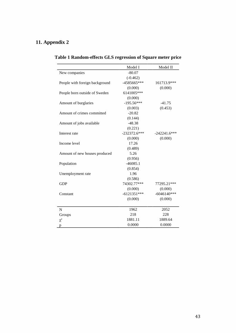
43
11. Appendix 2
Table 1 Random-effects GLS regression of Square meter price
Model I Model II
New companies -80.07
(-0.462)
People with foreign background -4585665*** 161713.9***
(0.000) (0.000)
People born outside of Sweden 6141005***
(0.000)
Amount of burglaries -195.56*** -41.75
(0.003) (0.453)
Amount of crimes committed -20.82
(0.144)
Amount of jobs available -48.38
(0.221)
Interest rate -232372.6*** -242241.6***
(0.000) (0.000)
Income level 17.26
(0.489)
Amount of new houses produced 5.26
(0.956)
Population -46085.1
(0.854)
Unemployment rate 1.96
(0.586)
GDP 74302.77*** 77295.21***
(0.000) (0.000)
Constant -6121351*** -6046140***
(0.000) (0.000)
N 1962 2052
Groups 218 228
χ² 1881.11 1889.64
p 0.0000 0.0000
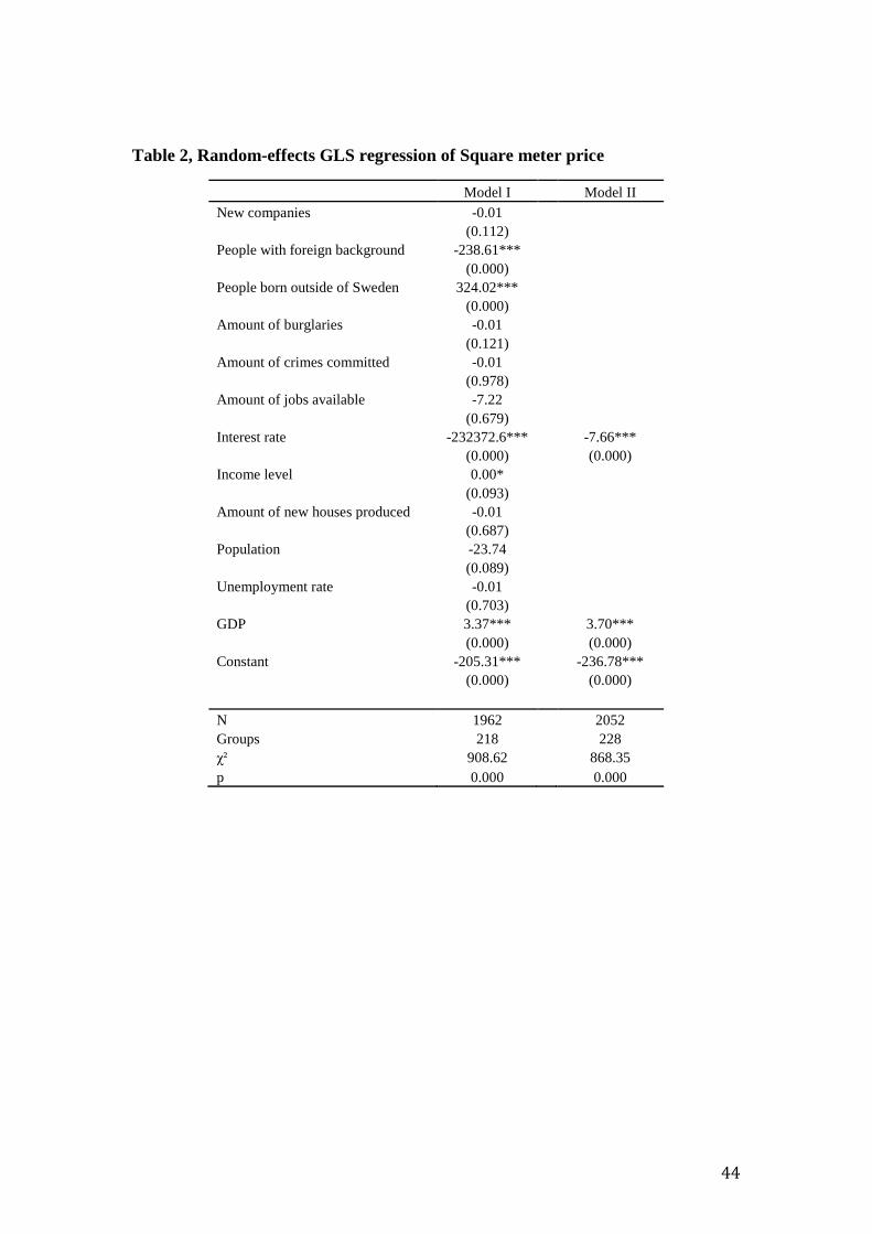
44
Table 2, Random-effects GLS regression of Square meter price
Model I Model II
New companies -0.01
(0.112)
People with foreign background -238.61***
(0.000)
People born outside of Sweden 324.02***
(0.000)
Amount of burglaries -0.01
(0.121)
Amount of crimes committed -0.01
(0.978)
Amount of jobs available -7.22
(0.679)
Interest rate -232372.6*** -7.66***
(0.000) (0.000)
Income level 0.00*
(0.093)
Amount of new houses produced -0.01
(0.687)
Population -23.74
(0.089)
Unemployment rate -0.01
(0.703)
GDP 3.37*** 3.70***
(0.000) (0.000)
Constant -205.31*** -236.78***
(0.000) (0.000)
N 1962 2052
Groups 218 228
χ² 908.62 868.35
p 0.000 0.000
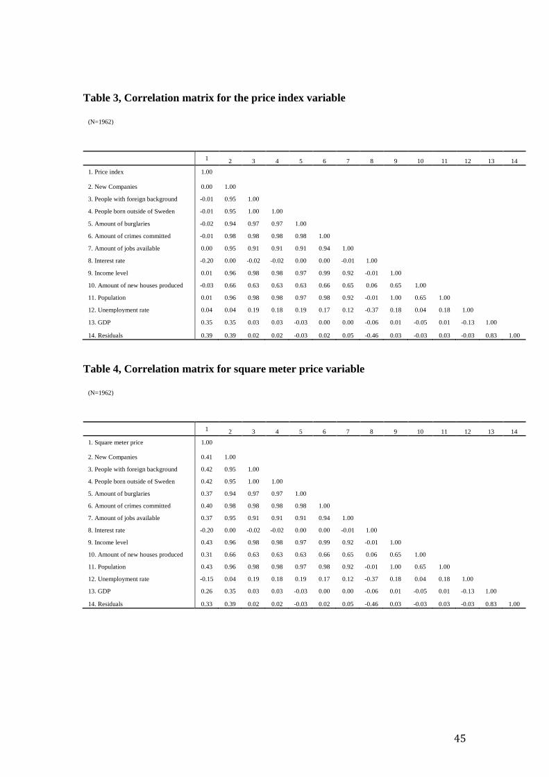
45
Table 3, Correlation matrix for the price index variable
(N=1962)
1 2 3 4 5 6 7 8 9 10 11 12 13 14
1. Price index 1.00
2. New Companies 0.00 1.00
3. People with foreign background -0.01 0.95 1.00
4. People born outside of Sweden -0.01 0.95 1.00 1.00
5. Amount of burglaries -0.02 0.94 0.97 0.97 1.00
6. Amount of crimes committed -0.01 0.98 0.98 0.98 0.98 1.00
7. Amount of jobs available 0.00 0.95 0.91 0.91 0.91 0.94 1.00
8. Interest rate -0.20 0.00 -0.02 -0.02 0.00 0.00 -0.01 1.00
9. Income level 0.01 0.96 0.98 0.98 0.97 0.99 0.92 -0.01 1.00
10. Amount of new houses produced -0.03 0.66 0.63 0.63 0.63 0.66 0.65 0.06 0.65 1.00
11. Population 0.01 0.96 0.98 0.98 0.97 0.98 0.92 -0.01 1.00 0.65 1.00
12. Unemployment rate 0.04 0.04 0.19 0.18 0.19 0.17 0.12 -0.37 0.18 0.04 0.18 1.00
13. GDP 0.35 0.35 0.03 0.03 -0.03 0.00 0.00 -0.06 0.01 -0.05 0.01 -0.13 1.00
14. Residuals 0.39 0.39 0.02 0.02 -0.03 0.02 0.05 -0.46 0.03 -0.03 0.03 -0.03 0.83 1.00
Table 4, Correlation matrix for square meter price variable
(N=1962)
1 2 3 4 5 6 7 8 9 10 11 12 13 14
1. Square meter price 1.00
2. New Companies 0.41 1.00
3. People with foreign background 0.42 0.95 1.00
4. People born outside of Sweden 0.42 0.95 1.00 1.00
5. Amount of burglaries 0.37 0.94 0.97 0.97 1.00
6. Amount of crimes committed 0.40 0.98 0.98 0.98 0.98 1.00
7. Amount of jobs available 0.37 0.95 0.91 0.91 0.91 0.94 1.00
8. Interest rate -0.20 0.00 -0.02 -0.02 0.00 0.00 -0.01 1.00
9. Income level 0.43 0.96 0.98 0.98 0.97 0.99 0.92 -0.01 1.00
10. Amount of new houses produced 0.31 0.66 0.63 0.63 0.63 0.66 0.65 0.06 0.65 1.00
11. Population 0.43 0.96 0.98 0.98 0.97 0.98 0.92 -0.01 1.00 0.65 1.00
12. Unemployment rate -0.15 0.04 0.19 0.18 0.19 0.17 0.12 -0.37 0.18 0.04 0.18 1.00
13. GDP 0.26 0.35 0.03 0.03 -0.03 0.00 0.00 -0.06 0.01 -0.05 0.01 -0.13 1.00
14. Residuals 0.33 0.39 0.02 0.02 -0.03 0.02 0.05 -0.46 0.03 -0.03 0.03 -0.03 0.83 1.00
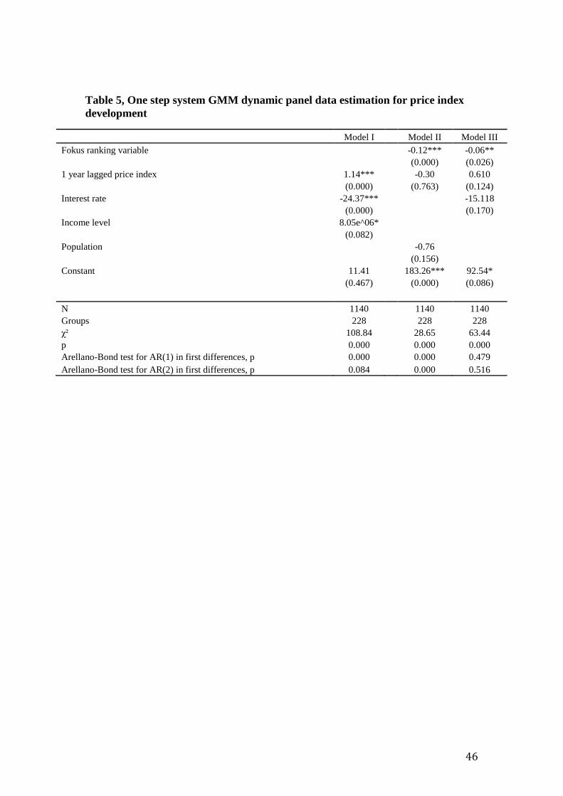
46
Table 5, One step system GMM dynamic panel data estimation for price index
development
Model I Model II Model III
Fokus ranking variable -0.12*** -0.06**
(0.000) (0.026)
1 year lagged price index 1.14*** -0.30 0.610
(0.000) (0.763) (0.124)
Interest rate -24.37*** -15.118
(0.000) (0.170)
Income level 8.05e^06*
(0.082)
Population -0.76
(0.156)
Constant 11.41 183.26*** 92.54*
(0.467) (0.000) (0.086)
N 1140 1140 1140
Groups 228 228 228
χ² 108.84 28.65 63.44
p 0.000 0.000 0.000
Arellano-Bond test for AR(1) in first differences, p 0.000 0.000 0.479
Arellano-Bond test for AR(2) in first differences, p 0.084 0.000 0.516
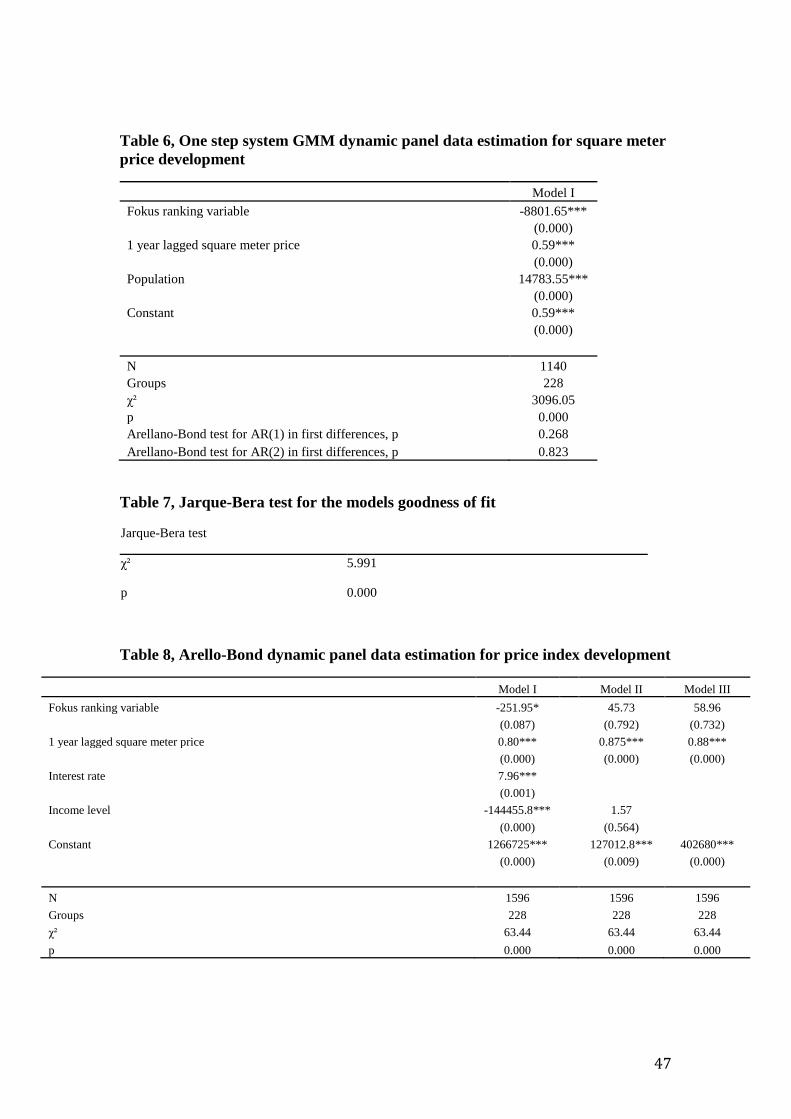
47
Table 6, One step system GMM dynamic panel data estimation for square meter
price development
Model I
Fokus ranking variable -8801.65***
(0.000)
1 year lagged square meter price 0.59***
(0.000)
Population 14783.55***
(0.000)
Constant 0.59***
(0.000)
N 1140
Groups 228
χ² 3096.05
p 0.000
Arellano-Bond test for AR(1) in first differences, p 0.268
Arellano-Bond test for AR(2) in first differences, p 0.823
Table 7, Jarque-Bera test for the models goodness of fit
Jarque-Bera test
χ² 5.991
p 0.000
Table 8, Arello-Bond dynamic panel data estimation for price index development
Model I Model II Model III
Fokus ranking variable -251.95* 45.73 58.96
(0.087) (0.792) (0.732)
1 year lagged square meter price 0.80*** 0.875*** 0.88***
(0.000) (0.000) (0.000)
Interest rate 7.96***
(0.001)
Income level -144455.8*** 1.57
(0.000) (0.564)
Constant 1266725*** 127012.8*** 402680***
(0.000) (0.009) (0.000)
N 1596 1596 1596
Groups 228 228 228
χ² 63.44 63.44 63.44
p 0.000 0.000 0.000