The Sustainable Debts of Philip II: A Reconstruction of Spain’s Fiscal Position, 1560-1598*

Mauricio Drelichman The University of British Columbia

and CIFAR

Hans-Joachim Voth ICREA/Universitat Pompeu Fabra

and CEPR

Abstract: The defaults of Philip II have attained mythical status as the origin of sovereign debt crises. The king failed to honor his debts four times during his reign. In this paper, we reassess the fiscal position of Habsburg Spain. New archival evidence allows us to derive comprehensive estimates of debt and revenue. These show that primary surpluses were sufficient to make the king’s debt sustainable for most of his reign. Spain’s debt burden was manageable up to the 1580s, and its fiscal position only deteriorated for good after the defeat of the “Invincible Armada.” We also estimate fiscal policy reaction functions, and show that Spain under the Habsburgs was at least as “responsible” as the US in the 20th century or as Britain in the 18th century. Our results suggest that the outcome of uncertain events such as wars may have more influence on a history of default than strict adherence to fiscal rules. JEL Classification Codes: H62, H63, F34, N24, N44

* For helpful comments, we thank Brian A’Hearn, Daron Acemoglu, Fernando Broner, Albert Carreras, Xavier Debrun, Marc Flandreau, Caroline Fohlin, Regina Grafe, Viktoria Hnatkovska, Alberto Martin, Paolo Mauro, David Mitch, Kris Mitchener, Joel Mokyr, Lyndon Moore, Roger Myerson, Kevin O’Rourke, Sevket Pamuk, Richard Portes, Angela Redish, Nathan Sussman, Alan M. Taylor, Francois Velde, Jaume Ventura, Marc Weidenmier, and Eugene White. Seminar audiences at American University, Harvard, Sciences Po, Hebrew University, UBC, UPF, UC Irvine, HEI Geneva, NYU-Stern, and Rutgers, as well as the EHA meetings in Austin, the CREI / CEPR Conference on “Crises – Past, Policy, and Theory”, CIFAR, NBER, CEPR –ESSIM, the BETA Workshop, and the Utrecht Workshop on Financial History offered advice and constructive criticism. Diego Pereira and Germán Pupato provided outstanding research assistance. Financial support from the Spanish Education Ministery, CREI, SSHRCC, UBC Hampton Fund, and TARGET/INE is gratefully acknowledged.

2

I. INTRODUCTION

Spain under the Habsburgs ruled an empire on which the sun never set. Her

financial troubles appear to have stretched every bit as far. Habsburg Spain was the first

“serial defaulter” in history (Reinhart, Rogoff, and Savastano 2003). Philip II failed to

honor his debts four times, in 1557, 1560, 1575 and 1596. Fernand Braudel (1966)

famously argued that only the indulgence of irrational bankers allowed Spain to incur

towering debts at a time when her fiscal position was deteriorating. When The Economist

writes about the origins of debt crises and the dangers of fiscal profligacy, it refers to

sixteenth century Spain.1 Fighting a series of expensive wars in a bid for European

hegemony, Spain’s public finances were heavily strained. Eventually, Spain went on to

hold the record for the total number of state bankruptcies. She failed to meet her

obligations 13 times between 1500 and 1900.2 There is also a widespread belief that

‘imperial overstretch’ led to Spain’s poor economic performance after 1600 (Kennedy

1987).3

Contrary to the received wisdom, we show that Philip II’s debts were

sustainable for most of his reign. The fiscal position did not deteriorate decisively until

the defeat of the ‘Invincible Armada’ in the late 1580s. Far from being undermined by

reckless spending and weak fiscal institutions, Spain’s finances suffered from

unexpected, large, negative shocks to her military position. Philip’s first three

bankruptcies were caused by temporary liquidity shocks, not structural revenue shortfalls.

1 “The dark side of debt”, The Economist, 21.9.2006. 2 Reinhart, Rogoff and Savastano (2003). 3 Spain’s poor long run economic performance has been most recently documented by Alvarez Nogal and Prados de la Escosura (2008).

3

Overall, Habsburg Spain’s fiscal discipline was similar to that of other hegemonic

powers, such as eighteenth-century Britain or twentieth-century America.

We provide the first comprehensive account of Philip II’s finances. Our yearly

estimates of fiscal variables, stretching from 1566 to 1596, are the earliest constructed for

a sovereign state in history. We start with a new data series on the Crown’s short-term

debts compiled from the Archive of Simancas. When combined with other existing data,

this series serves as the linchpin with which we reconstruct Philip II’s overall financial

position. We derive yearly estimates of revenues, debt service, primary surplus, budget

deficit, short-term borrowing and the stock of long-term debt. We also present new

estimates of the cost of financing for the Crown in several periods.

We use our estimates of Philip’s fiscal position to evaluate debt sustainability,

exploring the evolution of debt relative to GDP. Next, we estimate fiscal policy functions

in the style of Bohn (1998), and compare the results for Spain with those for 18th century

Britain and 20th century US. In combination, our findings suggest that earlier assessments

of Philip’s finances have been too pessimistic. We show that Habsburg Spain passes

several tests of fiscal sustainability, and actually conducted a more fiscally responsible

policy than the UK under Pitt. During the first three decades of Philip’s reign, Spanish

fiscal policy was even more ‘virtuous’ than that of the US between Woodrow Wilson and

Bill Clinton.

How could Philip II default so often and yet keep borrowing so much? Braudel

(1966) emphasized the role of gullible bankers. Conklin (1998) interpreted the

availability of funds in the style of the classic paper by Bulow and Rogoff (1989),

arguing that the ability of bankers to impose sanctions on the king was key. Genoese

4

lenders could stop the transfer of funds from Spain to the battlefields in the Netherlands,

forcing the king to settle his debts or risk the mutiny of unpaid armies. We do not

question that the ability to punish may have facilitated borrowing at certain critical

junctures. Rather, we argue that it was the overall health of Habsburg Spain’s fiscal

position and the responsiveness of the Crown’s taxing and spending behavior to rising

debt levels that made the continued flow of funds possible.

Our attempt to shed new light on the history of fiscal policy is related to a wider

research effort in recent years to expand our knowledge of early modern European state

finances. Reinhart, Rogoff and Savastano (2003) carefully reconstruct the long-run

history of debt and defaults since 1500. Bonney’s European State Finance Database

(Bonney 1995-2007) and the associated papers (Bonney 1999) represent a major effort to

compile a comprehensive overview of existing data sources. Other important

contributions in the same spirit include Hoffman and Norberg (1994), and W. M. Ormrod

et al. (1999). In combination, they offer insights into the “sinews of power” of almost

every nascent European national state. Spain, as one of the major players in the European

scene throughout most of modern history, has also attracted her share of scholarly

attention.4

We proceed as follows. In section II, we present our summary of Philip II’s

fiscal position, as it emerges from our new archival data. The sustainability of the debt

path is assessed in section III, using the traditional analytical tools such as the primary

surplus required to stabilize debt. Next, we estimate fiscal policy functions in the style of 4 For the sixteenth century, the classic works are Ruiz Martín (1965; 1968), Ulloa (1977), and Artola (1982). More recently Thompson (1994), Gelabert (1999), Marcos Martín (2000), Tortella and Comín (2001), Yun Casalilla (2002; 2004), and Alvarez Nogal and Prados de la Escosura (2008), have contributed much to our understanding of Spanish economic and fiscal history.

5

Bohn (1998), and offer some comparisons across time and space. The concluding section

discusses our main findings and puts them in context.

II. DATA

While her numerous defaults are widely cited in the literature on sovereign debt

crises, we know remarkably little about Spain’s overall fiscal position in the sixteenth

century. Existing evidence on tax revenues, expenditure, and debt is fragmentary. This is

a consequence of the decentralized nature and rudimentary information collection of

early modern states. Philip II himself – like most early modern rulers – did not have

access to consolidated figures of revenue, expenditure, or debt. Any attempt at estimating

them requires the painstaking assembly of disaggregated data sources and the careful use

of assumptions regarding the nature of missing data.

We first construct new revenue estimates by aggregating data from published

sources, and compare them with existing benchmark estimates. We then review the

characteristics of Spanish debt instruments, and introduce our new series of short-term

debt, constructed entirely from archival sources. Combined with existing estimates on

long-term bonds, we obtain yearly estimates of outstanding debt and the budget deficit.

Next, we use data on debt service costs to derive measures of revenue growth and

primary surplus for four different sub-periods. Finally, we feed these results into a simple

fiscal accounting framework to obtain yearly estimates of the fiscal position of Spain

between 1566 and 1596.5

5 Technically speaking, all our estimates use data on the kingdom of Castile. While Philip II ruled over many territories, it was Castile that financed his military enterprises and overseas empire. Philip also had

6

Revenues

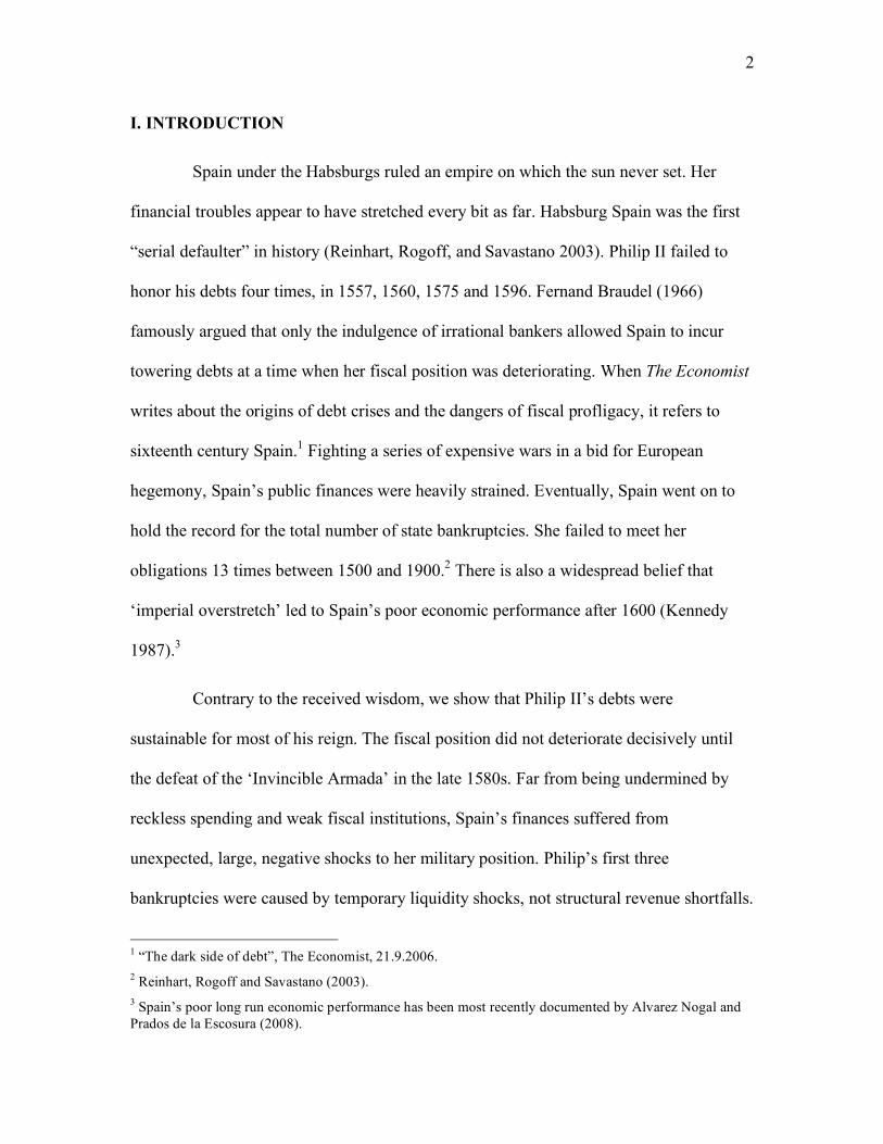
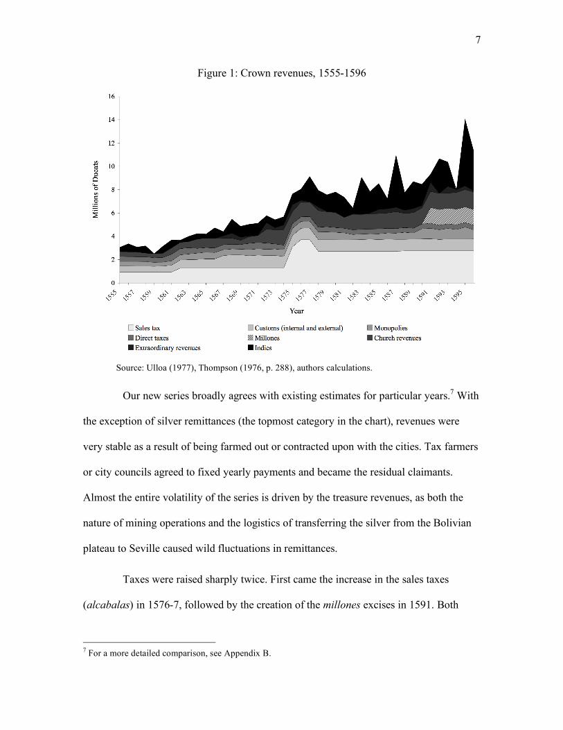
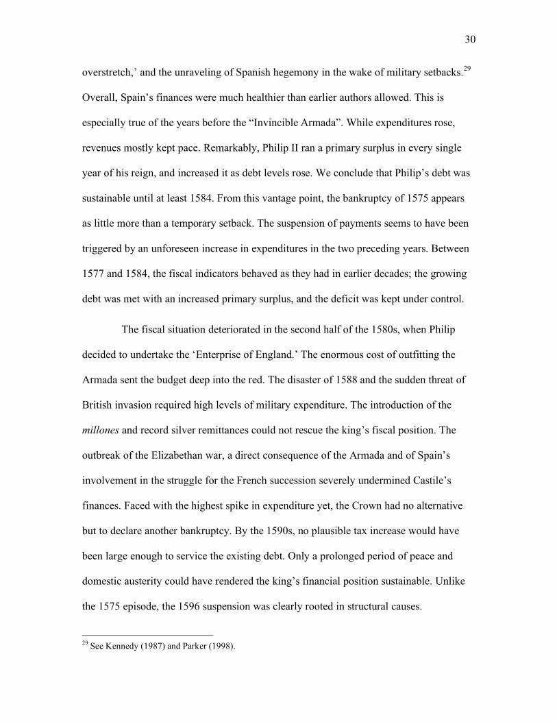
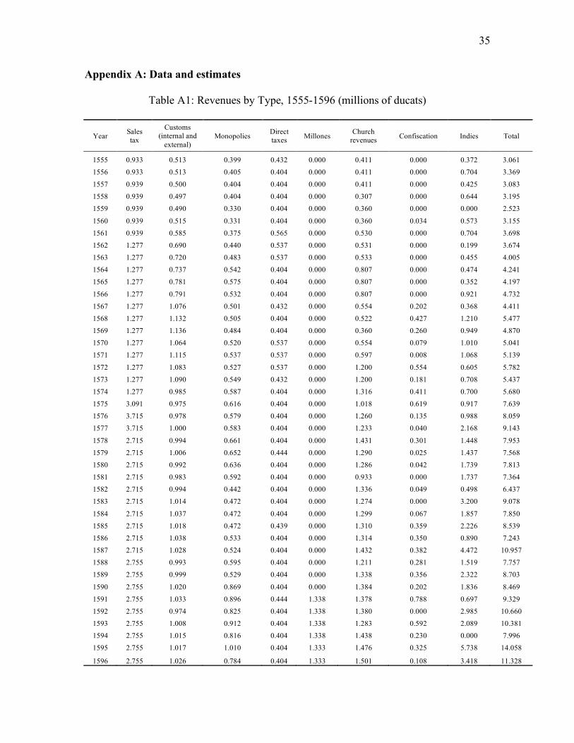
Figure 1 shows the evolution of Crown revenues by type between 1555 and

1596. While fragmentary data for individual tax streams are reported by Ulloa (1977) and

Thompson (1976), this is to our knowledge the first time that the different series have

been aggregated to produce a comprehensive annual series of fiscal income for this

period. For many revenue streams, data are incomplete. We impute missing observations

by assuming that, in years for which there is no information, revenues were equal to the

lower of the two closest years for which data was available. We have also incorporated

information on the frequency with which different taxes were collected when available.6

Table A1 in the appendix reports the data used in Figure 1.

much wider discretion over the use of Castilian revenues than over the resources of his other possessions (Drelichman and Voth 2008). For the remainder of the paper, we will use Castile and Spain interchangeably. 6 This procedure and Ulloa’s methodology bias the series downwards, yielding a lower bound of actual revenue. Since most of the revenue streams do not change for long periods, the actual impact of missing data turns out to be limited. Data for Indies revenue, the most volatile series, are available for every year throughout the period

7

Figure 1: Crown revenues, 1555-1596

Source: Ulloa (1977), Thompson (1976, p. 288), authors calculations.

Our new series broadly agrees with existing estimates for particular years.7 With

the exception of silver remittances (the topmost category in the chart), revenues were

very stable as a result of being farmed out or contracted upon with the cities. Tax farmers

or city councils agreed to fixed yearly payments and became the residual claimants.

Almost the entire volatility of the series is driven by the treasure revenues, as both the

nature of mining operations and the logistics of transferring the silver from the Bolivian

plateau to Seville caused wild fluctuations in remittances.

Taxes were raised sharply twice. First came the increase in the sales taxes

(alcabalas) in 1576-7, followed by the creation of the millones excises in 1591. Both

7 For a more detailed comparison, see Appendix B.

8

were introduced in the face of dire financial and military emergencies. The jump in sales

taxes followed the default of 1575 and the rapidly deteriorating situation in the

Netherlands. The hefty increase, front-loaded in the first two years, allowed Philip to

negotiate a settlement with his bankers, restart borrowing on a large scale, and resume

payments to his armies.8 The millones, a variety of new excises administered by the

cities, were introduced in response to the disaster of the Armada in 1588. They were

supposed to provide a one-time boost in revenue, spread over six years, to rebuild the

fleet and defuse the British threat. Nonetheless, they were renewed time and again and

became a permanent feature of Crown revenue. In both cases the king had to negotiate

with the Cortes, an assembly composed by representatives of the urban elites. In 1590 he

actually had to agree to a number of conditions imposed by the cities in order to obtain

their consent.9

Debt

The Spanish Crown borrowed using two main instruments: asientos and juros

(short and long-term loans, respectively). Since our reconstruction of the Spanish fiscal

position in the second half of the sixteenth century hinges on the relationship between

these instruments, we describe them in more detail.

8 For an account of the king’s negotiations with the Cortes of 1576 that led to the increase in the alcabalas see Jago (1985). 9 The Cortes nonetheless failed to transform their temporary bargaining strength into permanent political gains. For a thorough discussion of the effect of silver revenues on the interaction between king and Cortes see Drelichman and Voth (2008).

9

Characteristics and chronology

Asientos were short-term loans contracted with individual bankers or companies.

Their term typically ranged from six months to three years. When the contracts called for

disbursements abroad, usually to pay and supply warring armies and fleets, the stipulated

exchange rate was normally used to increase the effective interest rate while

circumventing usury laws. During Philip’s reign, asientos usually included a license to

export bullion from Castile, as well as clauses protecting the bankers against variations in

the metallic content of the currency.

Juros were long-term bonds secured against a particular revenue stream, such as

the sales taxes of the city of Seville. Juros were normally perpetual, although lifetime

bonds were not uncommon. While interest on juros could only be collected by the person

in whose name they had been issued, a secondary market of sorts in them existed. The

Crown was all too willing to grant licenses to transfer them in exchange for fees, loans or

other favors. Since their annual or semi-annual interest payments were directly disbursed

by the treasurer or tax farmer in control of the revenue stream that guaranteed the bond,

the value of a juro was directly related to the liquidity and reliability of that particular

revenue stream.10

While Charles V assiduously serviced his loans with German bankers, Philip did

not go to the same lengths. Barely a year after ascending to the throne, he defaulted on

outstanding asientos. His first debt rescheduling unfolded in two stages in 1557 and

1560. The settlement, which included handing over control of several Crown monopolies

10 The market for juros remains a fertile area for research. A good overview is provided by Toboso Sánchez (1987).

10

to the Fugger bank, was not fully negotiated until 1566. In that year lending resumed in

earnest. 1566 also marked the resumption of large military commitments abroad. The

Dutch Revolt flared up, and Spain began to build up the Mediterranean fleet that would

defeat the Ottomans at Lepanto in 1571. The Genoese asientos that financed these and

other expenses differed from those previously extended by German bankers. Many were

collateralized through juros. In the first few years after 1566 the bankers held onto these

juros (called de resguardo, or safeguards) until the asiento was repaid. Soon, however,

many asientos allowed the bankers to sell the collateral on the secondary market, even

when the asiento guaranteed by it was in good standing.11 When an inventory of the

outstanding asientos and juros was taken prior to the negotiations to settle the suspension

of payments of 1575, it was found that about two thirds of outstanding short-term loans

were collateralized by juros.12

The crisis of 1575 is possibly the single most studied episode in sixteenth

century Spanish financial history.13 The Dutch Revolt and the Mediterranean campaign

had put severe strain on the royal finances. These were compounded by the cost of the

gigantic palace-monastery at El Escorial. When Philip asked for a threefold increase in

the sales taxes that were the mainstay of fiscal revenue, the Cortes, in the first show of

force in half a century, refused to oblige.14 While the king eventually managed to obtain a

large increase in revenues, it came too late to avoid a suspension of payments on

11 For a description of the interplay of asientos and juros see Ruíz Martín (1965). 12 This number emerges from our calculations based on the full text of the final settlement with the bankers. Asiento y Medio General de la Hacienda. Archivo General de Simancas; Consejo y Juntas de Hacienda; Libro 42. See Appendix B for a detailed analysis. 13 For a meticulous description of the suspension and ensuing settlement see Lovett (1980; 1982). 14 Jago (1985).

11

asientos, as well as on collateral juros still held by the bankers. The total outstanding

amount was roughly 15 million ducats, or two years’ worth of revenue. Five and a half

million ducats had been collateralized through standard juros, while 4.3 million were

backed by juros guaranteed by the Casa de Contratación that had failed to perform as

expected and were already trading at a heavy discount.15

Two years of negotiations with the bankers produced a comprehensive

settlement, known as a medio general, which converted all the outstanding short-term

loans to low interest perpetuities. Appendix C details the restructuring based on the

original text of the settlement. On average, the king repaid 62 cents on the dollar. The

bankers also agreed to immediately provide a new loan of five million ducats. Fresh

lending started quickly, in 1578.

Lending proceeded briskly in the last quarter of the century. Philip’s fourth

suspension of payments, in 1596, was mild when compared to the 1575 default. The

medio general of 1597 rescheduled 7.04 million ducats, about two thirds of yearly

revenue. Two thirds of outstanding debt was converted to 5% juros, and the rest was

repaid in full through a juros swap. On average the king repaid 81 cents on the dollar.16

A new series of asientos

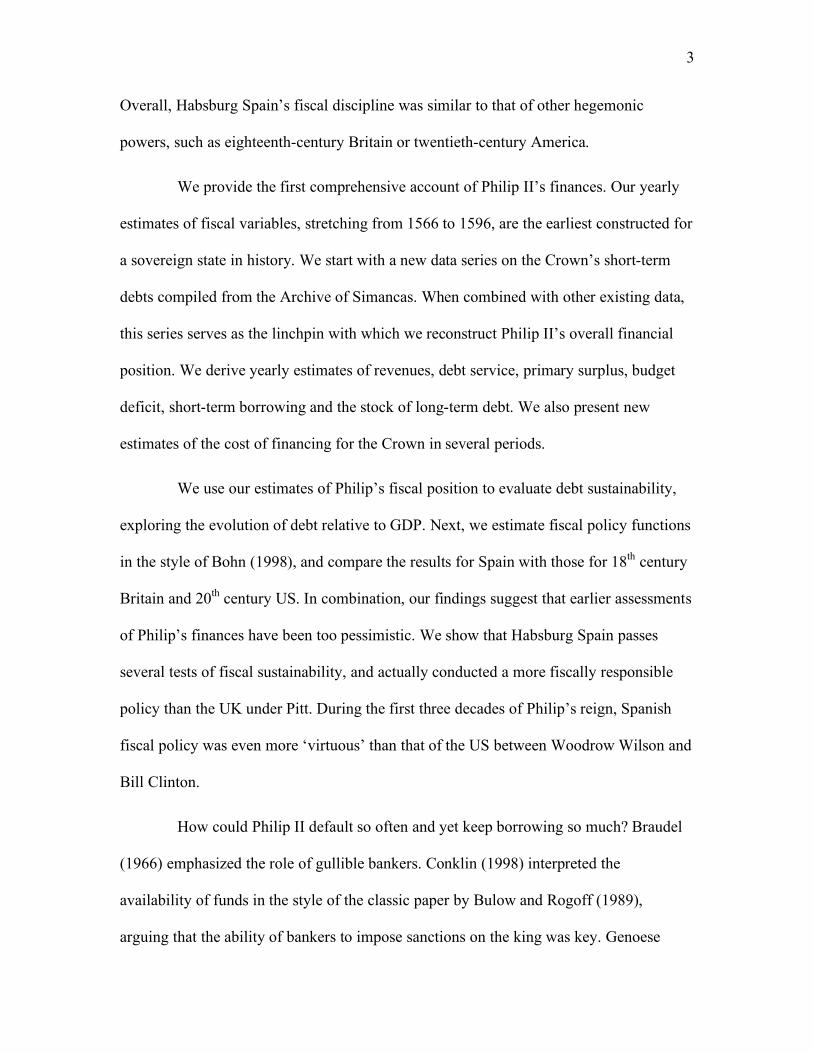
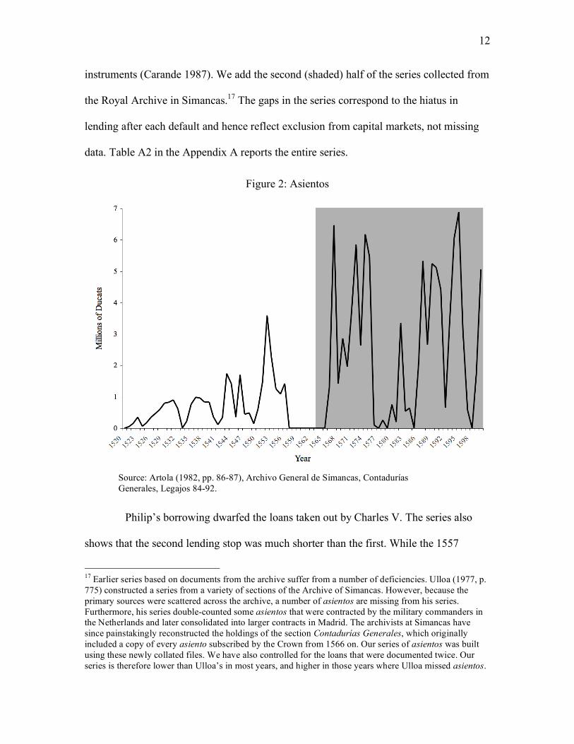
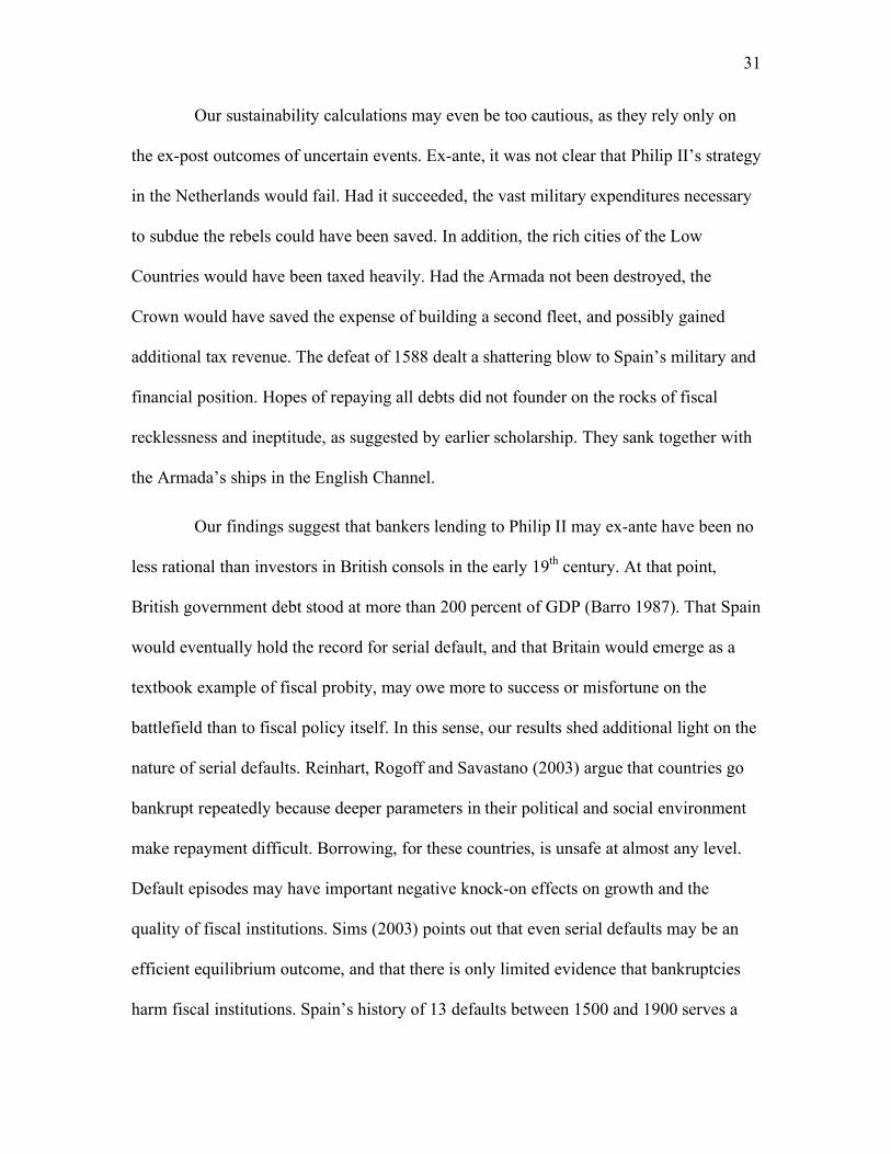
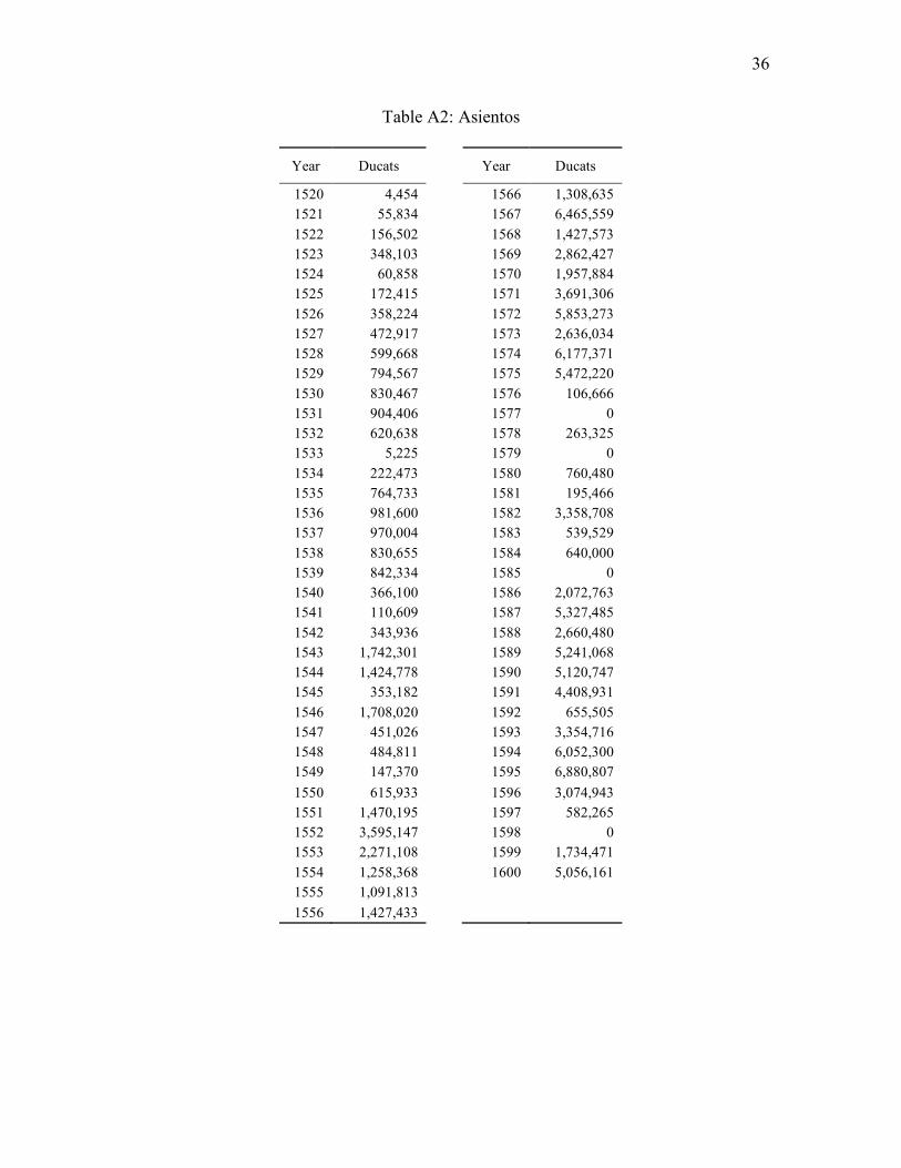
Figure 2 shows the value of new asientos contracted by the Crown between

1520 and 1600. The data for 1520-1555 comes from Ramón Carande’s three-volume

Carlos V y sus banqueros, which pioneered the study of sixteenth century Castilian debt

15 Juros guaranteed by the House of Trade, perhaps the most spectacular case of financial mismanagement during Philip’s reign, were thoroughly studied by Ruíz Martín (1965). 16 For details, see Appendix C.

12

instruments (Carande 1987). We add the second (shaded) half of the series collected from

the Royal Archive in Simancas.17 The gaps in the series correspond to the hiatus in

lending after each default and hence reflect exclusion from capital markets, not missing

data. Table A2 in the Appendix A reports the entire series.

Figure 2: Asientos

Source: Artola (1982, pp. 86-87), Archivo General de Simancas, Contadurías Generales, Legajos 84-92.

Philip’s borrowing dwarfed the loans taken out by Charles V. The series also

shows that the second lending stop was much shorter than the first. While the 1557

17 Earlier series based on documents from the archive suffer from a number of deficiencies. Ulloa (1977, p. 775) constructed a series from a variety of sections of the Archive of Simancas. However, because the primary sources were scattered across the archive, a number of asientos are missing from his series. Furthermore, his series double-counted some asientos that were contracted by the military commanders in the Netherlands and later consolidated into larger contracts in Madrid. The archivists at Simancas have since painstakingly reconstructed the holdings of the section Contadurías Generales, which originally included a copy of every asiento subscribed by the Crown from 1566 on. Our series of asientos was built using these newly collated files. We have also controlled for the loans that were documented twice. Our series is therefore lower than Ulloa’s in most years, and higher in those years where Ulloa missed asientos.

13

default resulted in nine years of exclusion from capital markets, most of the debt

suspended in 1575 was rescheduled through the medio general by late 1577.

The amounts borrowed through asientos during Philip’s reign also show very

large year-to-year variations relative to trend. Asientos were convenient as a short-term

borrowing device; they allowed the Crown to obtain money quickly and transfer it to

virtually any point in its European dominions. They were also expensive. It was not

uncommon for the cost of an asiento to climb into the double digits, with some possibly

yielding more than 20% per annum.18 As soon as it could, the Crown sought to convert

the outstanding amount into juros, which could be placed at interest rates around 7%. The

interest rates paid by Philip II are not dissimilar to those prevalent for contracts with the

same maturities elsewhere in Europe (Homer and Sylla 2005, p. 119). The series of

asientos can be interpreted as reflecting the flow of new borrowing; to estimate

outstanding debt, one needs to look at juros.19

18 Establishing the cost of borrowing is no trivial matter, as it involves estimates of the value of export licenses, hidden interest rate charges for transfer services, and the like. We are currently engaged in a large-scale project that will produce detailed estimates of the cost of each asiento. The following are examples of this coding endeavor: in an asiento underwritten by Niccoló and Vincenzo Cattaneo on December 5 1567 for a disbursement of 75,000 ducats, the king agreed to repayments in cash and juros, as well as juro swaps, that represented a total cost of financing of 40.77%. In another asiento underwritten by Juan Curiel de la Torre on December 15 1567 for a total of 200,000 ecús to be delivered in Anvers, the king agreed to exchange and interest charges and to the concession of lifetime juros that amounted to a total cost of financing of 29.44%. (Archivo General de Simancas, Contadurías Generales, Legajo 84). While in many cases the cost of financing was much lower, juros could be normally placed at around 7% and their capital was never due, representing a much more attractive option if revenues to guarantee them could be found. 19 The borrowing system shares some similarities with the Navy and Army bills used in 18th century Britain, which were used for (expensive) short-term borrowing, and were later consolidated into long-term consols (Dickson 1967).

14

Constructing estimates of outstanding debt

Because there are no reliable expenditure data, obtaining estimates of total

outstanding debt is crucial for reconstruction Spain’s fiscal position. We begin by

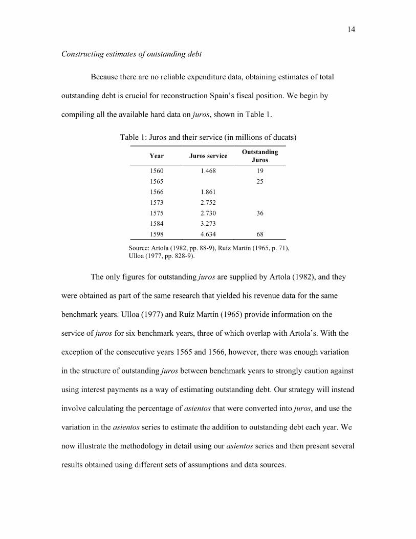
compiling all the available hard data on juros, shown in Table 1.

Table 1: Juros and their service (in millions of ducats)

Year Juros service Outstanding Juros

1560 1.468 19 1565 25 1566 1.861 1573 2.752 1575 2.730 36 1584 3.273 1598 4.634 68

Source: Artola (1982, pp. 88-9), Ruíz Martín (1965, p. 71), Ulloa (1977, pp. 828-9).

The only figures for outstanding juros are supplied by Artola (1982), and they

were obtained as part of the same research that yielded his revenue data for the same

benchmark years. Ulloa (1977) and Ruíz Martín (1965) provide information on the

service of juros for six benchmark years, three of which overlap with Artola’s. With the

exception of the consecutive years 1565 and 1566, however, there was enough variation

in the structure of outstanding juros between benchmark years to strongly caution against

using interest payments as a way of estimating outstanding debt. Our strategy will instead

involve calculating the percentage of asientos that were converted into juros, and use the

variation in the asientos series to estimate the addition to outstanding debt each year. We

now illustrate the methodology in detail using our asientos series and then present several

results obtained using different sets of assumptions and data sources.

15

We begin with the period 1565 – 1575. Artola’s data tells us that in 1575, just

before Philip’s third bankruptcy, the royal auditors found 36 million ducats in

outstanding juros. These included the juros de resguardo that collateralized a fraction of

the outstanding asientos. From the text of the settlement implemented through the medio

general we also know that in 1575 there were 4,644,139 ducats of outstanding asientos

that were not collateralized by juros.20 The total outstanding debt in 1575 was therefore

40.6 million ducats.

The next step is to calculate what percentage of asientos were repaid on average,

and what fraction were converted into juros. We know that in 1565 there were few or no

outstanding asientos, as short-term lending had not yet resumed. From our series, we also

know that between 1565 and 1575, the Crown borrowed a total of 37.852 million ducats

through asientos. Finally, by taking the difference in the stock of outstanding juros

between 1575 and 1565, we know that 11 million ducats worth of asientos were

converted into juros, while the rest were repaid. This implies that, on average, 29.06% of

asientos were converted into juros in this period. We estimate the outstanding debt each

year by adding 29.06% of the asientos underwritten the previous year to the existing

stock of juros. Our assumption is therefore that in each year the conversion ratio equaled

the average for the entire period. This reduces the volatility in the true path of debt;

however, it will not introduce persistent deviations from the true value of outstanding

debt, as the series must always converge to the benchmark year observations.

20 Asiento y Medio General de la Hacienda. Archivo General de Simancas; Consejo y Juntas de Hacienda; Libro 42.

16

To calculate the path of debt between 1575 and 1598 we employ the same

methodology, taking care to account for the effects of the 1575 and 1596 defaults. The

path of debt also depends on how one calculates the write-off imposed on bankers in each

default. We employ two different strategies. The first (face value) approach consists in

valuing debt conversions at face value, much like it would have appeared in official

books; the second (market value) approach estimates the reduction in the market value of

debt imposed through reductions in the annuity rate, that is, the opportunity cost incurred

by the bankers. Since the defaults always implied a swap of debt instruments of equal

face value (but often with different maturities and annuity rates), the face value approach

implies that, at least on paper, there were no haircuts.21 Under the market value approach

outstanding debt was reduced by 5.5 million ducats in the 1575 default and by 1.4 million

ducats in the 1596 bankruptcy. Appendix C discusses the settlements in detail and shows

how we obtain the value of the write-offs necessary to calculate the path of debt using the

market value approach to defaults.

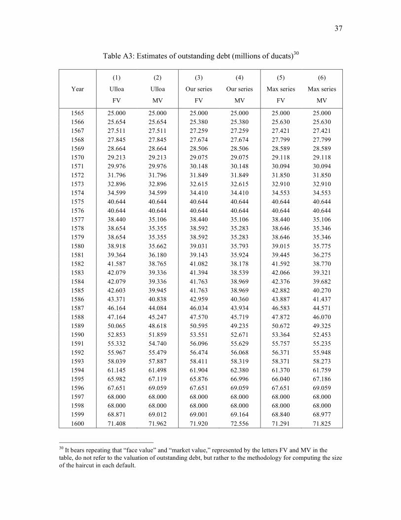
In order to assess the effects of our assumptions and data, we combine the face

value and market value approaches with three different series of asientos. The first series

is our own, the second is Ulloa’s, and the third is constructed by taking the maximum

value between our series and Ulloa’s for each year. This yields six different estimates for

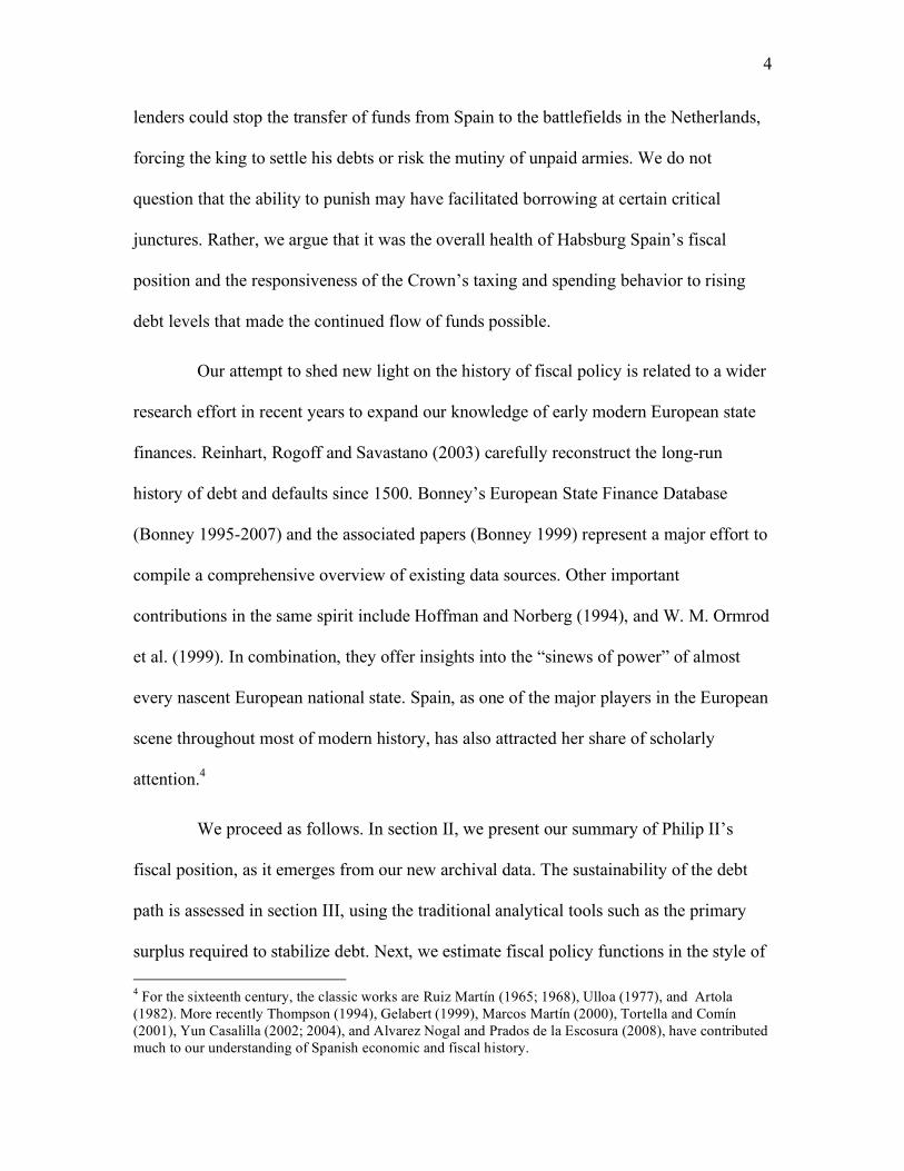
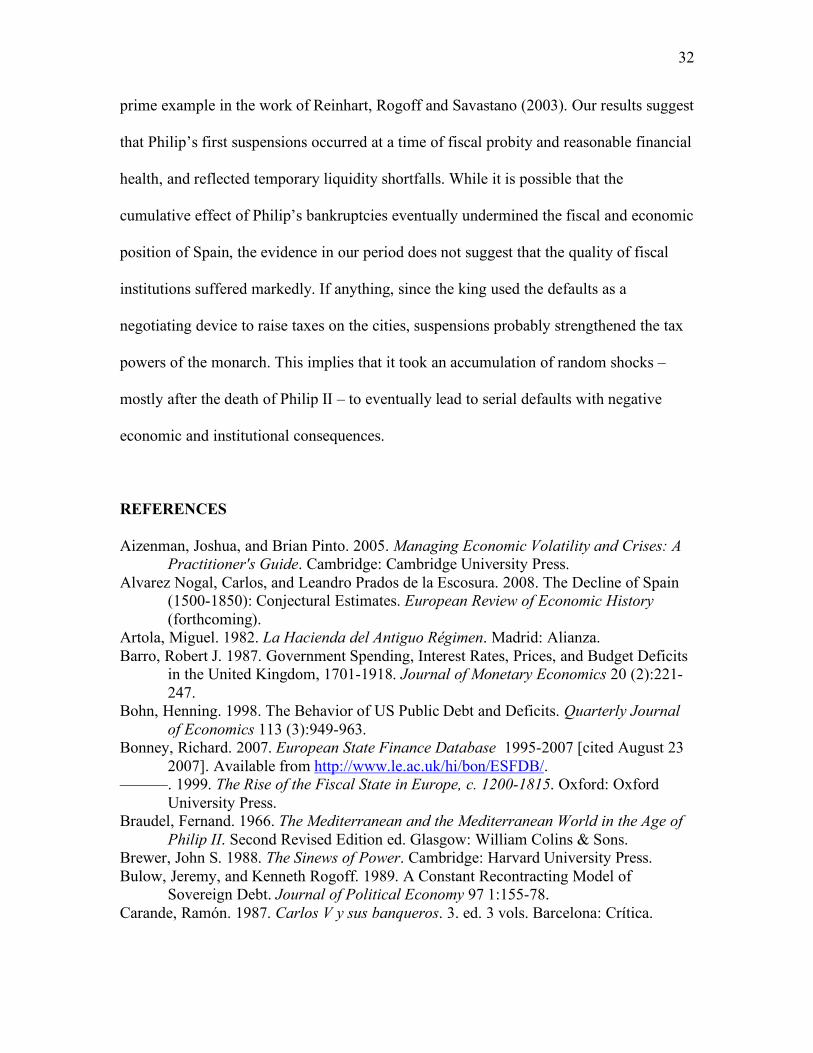
the path of debt, which we report in Table A3 in appendix A. Figure 3 shows the

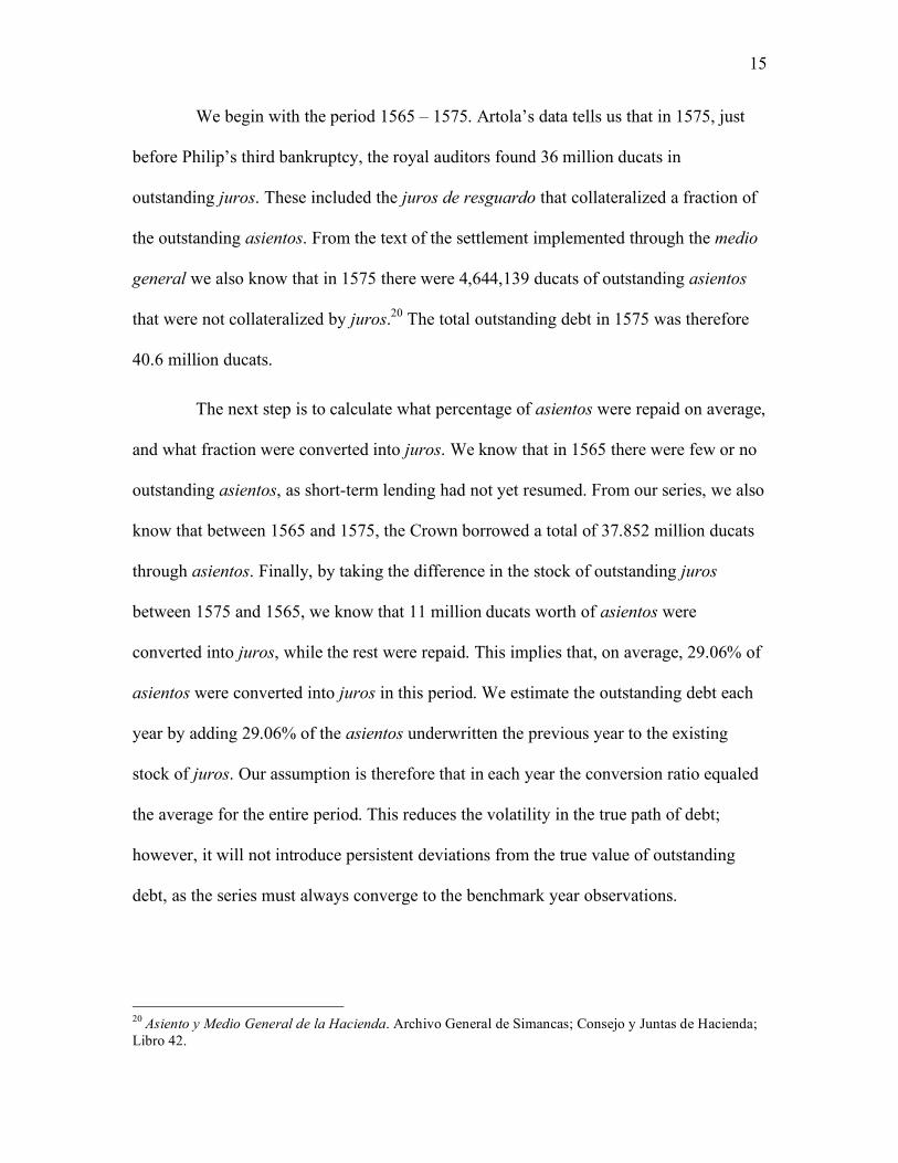
estimates that yield the highest and lowest paths of debt; the dotted line is obtained using

21 This difficulty is common to many historical estimations of the debt burden (Barro 1987). While the face value approach might appear a less convincing way of estimating debt, it has two ready uses. The first one is to provide an upper bound for the true value of debt. More importantly for our purposes, it also provides a debt path that does not reflect the haircut imposed on bankers. This will be crucial in our estimation of fiscal response functions, where interpreting a haircut as a sign of fiscal responsibility would bias the results in our favor.

17

the maximum asientos series and the face value approach to defaults; the solid line is

derived from our own series of asientos and the market value approach.

Figure 3: Upper and lower bound estimates of outstanding debt (millions of ducats)

Source: see the text.

The paths differ in the 1577 – 1591 period. At its 1585 maximum, the difference

is almost 4 million ducats, or 10% of outstanding debt.

Budget deficit

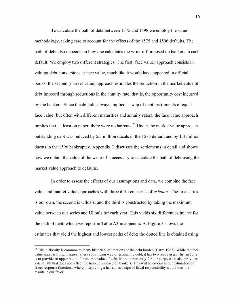
Our estimates of outstanding debt allow us to calculate a series for the budget

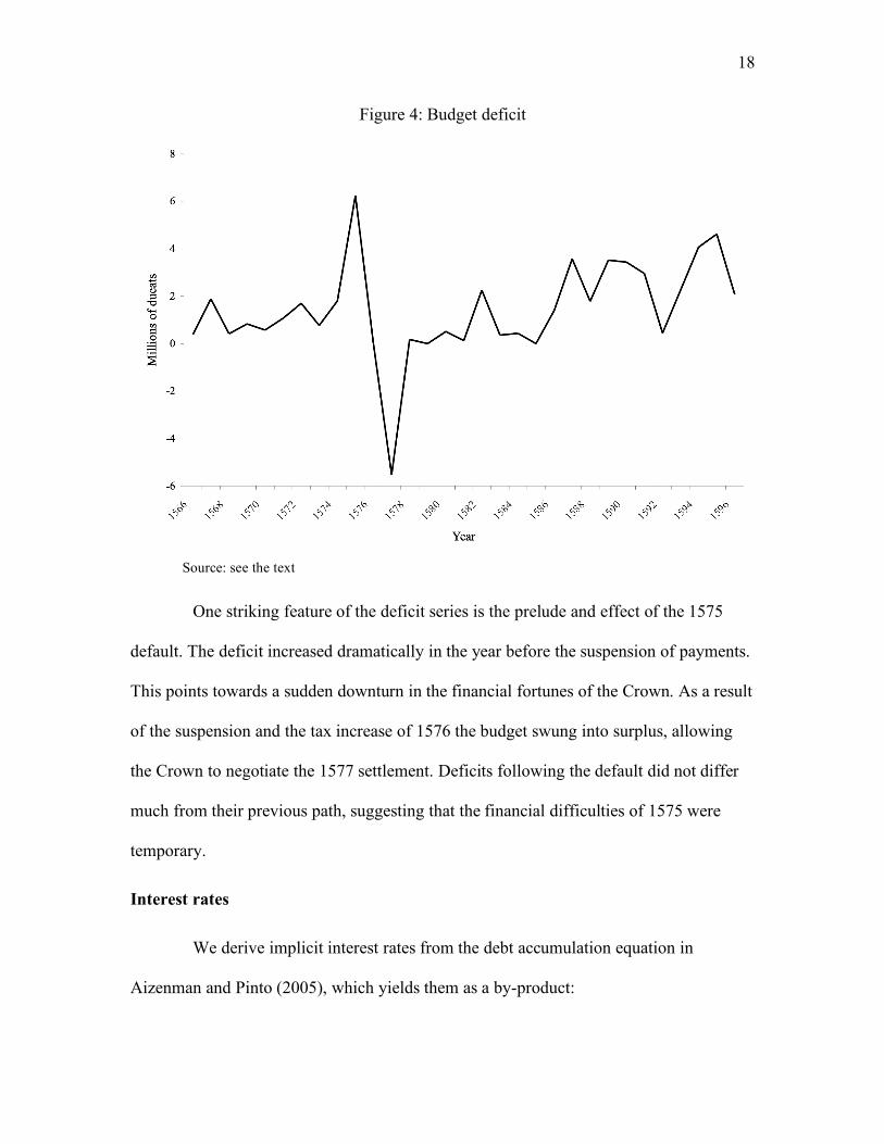
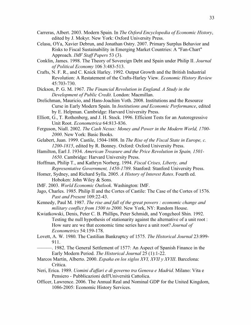
deficit, which by definition is the increase in the stock of debt. Figure 4 shows the deficit

series based on the debt path calculated using our own data and the market value

approach to defaults.

18

Figure 4: Budget deficit

Source: see the text

One striking feature of the deficit series is the prelude and effect of the 1575

default. The deficit increased dramatically in the year before the suspension of payments.

This points towards a sudden downturn in the financial fortunes of the Crown. As a result

of the suspension and the tax increase of 1576 the budget swung into surplus, allowing

the Crown to negotiate the 1577 settlement. Deficits following the default did not differ

much from their previous path, suggesting that the financial difficulties of 1575 were

temporary.

Interest rates

We derive implicit interest rates from the debt accumulation equation in

Aizenman and Pinto (2005), which yields them as a by-product:

19

!

"dt = #pst +(rt # gt )

(1+ gt )dt#1 (1)

where Δd is the change in the debt to GDP ratio, ps is the primary surplus as a percentage

of GDP, r is the (nominal) rate of interest, and g is the growth rate of GDP.

Estimates of 16th century Spanish GDP differ enormously. We interpolate Albert

Carreras’ (2003) estimates for Castile, the fiscal unit of interest.22 We will focus on four

periods: 1560-65, 1565-75, 1577-84 and 1584-96. This will allow us to use only hard

data for debt service (the six benchmark observations reported in Table 1) as well as to

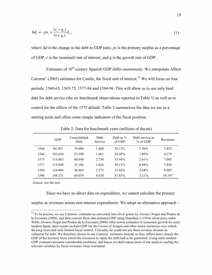
control for the effects of the 1575 default. Table 2 summarizes the data we use as a

starting point and offers some simple indicators of the fiscal position.

Table 2: Data for benchmark years (millions of ducats)

GDP Consolidated

Debt Debt

Service Debt as %

of GDP Debt service as

% of GDP Revenues

1560 94.307 19.000 1.468 20.15% 1.56% 3.035 1566 103.624 25.380 1.861 24.49% 1.80% 4.379 1575 113.083 40.644 2.730 35.94% 2.41% 7.093 1577 115.049 35.106 1.024 30.51% 0.89% 7.850 1584 124.006 38.969 3.273 31.43% 2.64% 8.005 1596 144.331 69.059 4.634 47.85% 3.21% 10.197

Source: see the text.

Since we have no direct data on expenditure, we cannot calculate the primary

surplus as revenues minus non-interest expenditures. We adopt an alternative approach –

22 To be precise, we use Carreras’ estimates as converted into silver grams by Alvarez Nogal and Prados de la Escosura (2008), and then convert them into nominal GDP using Hamilton’s (1934) silver price index. While Alvarez Nogal and Prados de la Escosura (2008) offer newer estimates of economic growth for early modern Spain, their results include GDP for the Crown of Aragon and other minor territories over which the king exercised only limited fiscal control. Crucially, he could not use these revenue streams as collateral for debt. We therefore choose to use Carreras’ estimates instead, as they reflect more closely the GDP of the territory from which the resources to repay the debt had to be generated. Using early modern GDP estimates presents considerable problems, and hence we shall repeat parts of our analysis scaling the relevant variables by fiscal revenues when warranted.

20

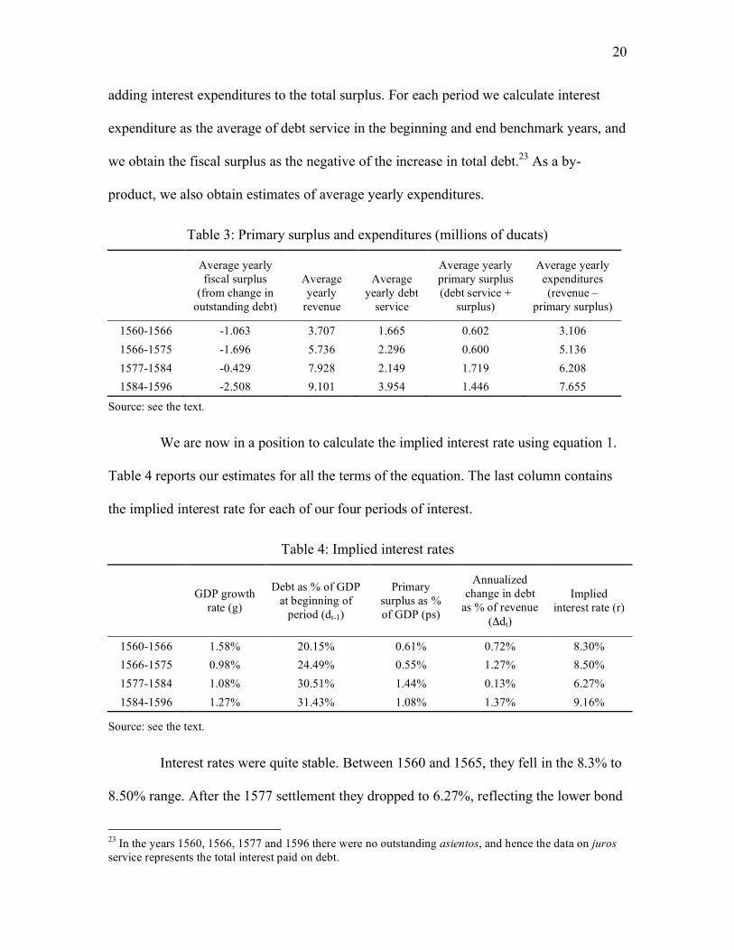
adding interest expenditures to the total surplus. For each period we calculate interest

expenditure as the average of debt service in the beginning and end benchmark years, and

we obtain the fiscal surplus as the negative of the increase in total debt.23 As a by-

product, we also obtain estimates of average yearly expenditures.

Table 3: Primary surplus and expenditures (millions of ducats)

Average yearly fiscal surplus

(from change in outstanding debt)

Average yearly

revenue

Average yearly debt

service

Average yearly primary surplus (debt service +

surplus)

Average yearly expenditures (revenue –

primary surplus)

1560-1566 -1.063 3.707 1.665 0.602 3.106 1566-1575 -1.696 5.736 2.296 0.600 5.136 1577-1584 -0.429 7.928 2.149 1.719 6.208 1584-1596 -2.508 9.101 3.954 1.446 7.655

Source: see the text.

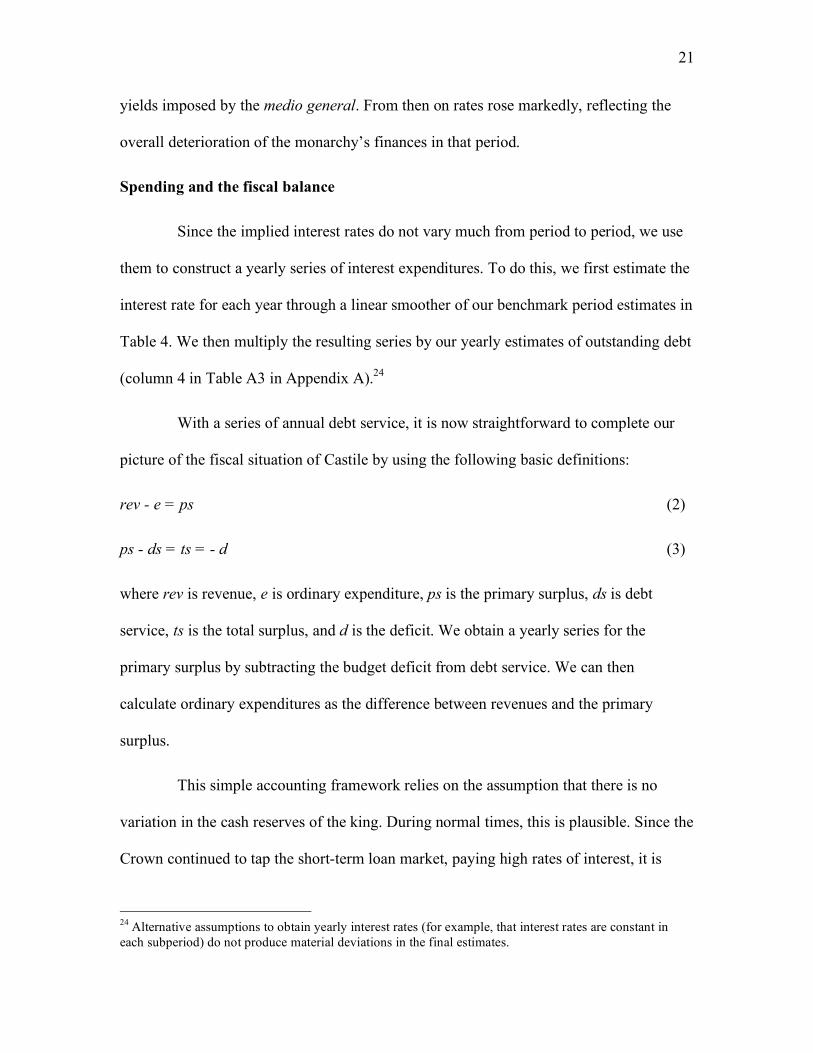
We are now in a position to calculate the implied interest rate using equation 1.

Table 4 reports our estimates for all the terms of the equation. The last column contains

the implied interest rate for each of our four periods of interest.

Table 4: Implied interest rates

GDP growth rate (g)

Debt as % of GDP at beginning of

period (dt-1)

Primary surplus as % of GDP (ps)

Annualized change in debt

as % of revenue (Δdt)

Implied interest rate (r)

1560-1566 1.58% 20.15% 0.61% 0.72% 8.30% 1566-1575 0.98% 24.49% 0.55% 1.27% 8.50% 1577-1584 1.08% 30.51% 1.44% 0.13% 6.27% 1584-1596 1.27% 31.43% 1.08% 1.37% 9.16%

Source: see the text.

Interest rates were quite stable. Between 1560 and 1565, they fell in the 8.3% to

8.50% range. After the 1577 settlement they dropped to 6.27%, reflecting the lower bond

23 In the years 1560, 1566, 1577 and 1596 there were no outstanding asientos, and hence the data on juros service represents the total interest paid on debt.

21

yields imposed by the medio general. From then on rates rose markedly, reflecting the

overall deterioration of the monarchy’s finances in that period.

Spending and the fiscal balance

Since the implied interest rates do not vary much from period to period, we use

them to construct a yearly series of interest expenditures. To do this, we first estimate the

interest rate for each year through a linear smoother of our benchmark period estimates in

Table 4. We then multiply the resulting series by our yearly estimates of outstanding debt

(column 4 in Table A3 in Appendix A).24

With a series of annual debt service, it is now straightforward to complete our

picture of the fiscal situation of Castile by using the following basic definitions:

rev - e = ps (2)

ps - ds = ts = - d (3)

where rev is revenue, e is ordinary expenditure, ps is the primary surplus, ds is debt

service, ts is the total surplus, and d is the deficit. We obtain a yearly series for the

primary surplus by subtracting the budget deficit from debt service. We can then

calculate ordinary expenditures as the difference between revenues and the primary

surplus.

This simple accounting framework relies on the assumption that there is no

variation in the cash reserves of the king. During normal times, this is plausible. Since the

Crown continued to tap the short-term loan market, paying high rates of interest, it is

24 Alternative assumptions to obtain yearly interest rates (for example, that interest rates are constant in each subperiod) do not produce material deviations in the final estimates.

22

unlikely that it maintained or increased its cash reserves. During a default, however, the

king must have held cash reserves (which we do not observe) to meet his expenditure

needs, as borrowing was not available. The logic of our accounting exercise lumps any

increase in cash reserves together with expenditure. We thus overestimate expenditure

during the year of the default, when the king is building up his cash reserves. Conversely,

since we do not observe expenditure financed by running down cash reserves, we also

underestimate outlays in the year of the settlement. This problem affects the values for

the years 1575, 1576 and 1577. Since we have the correct value for the sum of these three

years, we imputed 1/3 of the total to each of them. We then adjusted the primary surplus

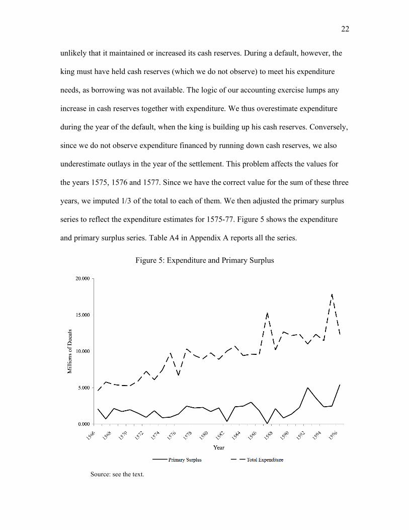
series to reflect the expenditure estimates for 1575-77. Figure 5 shows the expenditure

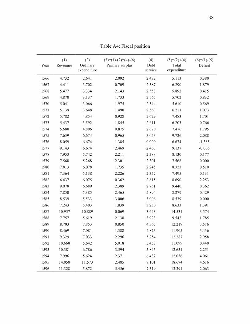
and primary surplus series. Table A4 in Appendix A reports all the series.

Figure 5: Expenditure and Primary Surplus

Source: see the text.

23

From Figure 5 it is immediately apparent that Philip II managed to run a primary

surplus in every year of his reign for which we have data. The king never borrowed to

cover interest. It is also evident that, despite large fluctuations mostly related to silver

revenues, the average primary surplus increased throughout the period as the Crown

strove to deal with the increasing interest payments. The expenditure series displays the

battle scars of Spanish financial and military policy. It is easy to distinguish the stop of

interest payments in 1576, the enormous expenses to outfit the Armada in 1588, and the

outbreak of the last phase of the Elizabethan war, which Spain fought against France and

England between 1595 and 1598.

III. SUSTAINABILITY

Traditional sustainability analysis

What is a sustainable level of debt? According to one approach, for spending

and borrowing to be sustainable, the long-run level of the debt to GDP ratio has to be

stable (IMF 2003). An explosion of debt can be avoided if a government effectively does

not borrow to pay interest, and reserves a substantial portion of its regular income for

debt servicing. In other words, debt sustainability requires that the primary surplus be

high enough to render equation 1 at least equal to zero, implying ps ≥ ps*. Table 5

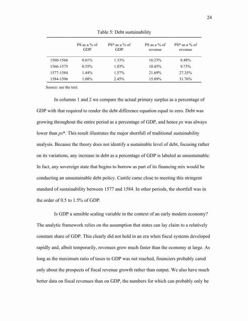
summarizes the traditional debt sustainability analysis for sixteenth century Castile.

24

Table 5: Debt sustainability

PS as a % of GDP

PS* as a % of GDP

PS as a % of revenue

PS* as a % of revenue

1560-1566 0.61% 1.33% 16.23% 8.48% 1566-1575 0.55% 1.83% 10.45% 9.73% 1577-1584 1.44% 1.57% 21.69% 27.35% 1584-1596 1.08% 2.45% 15.89% 31.76%

Source: see the text.

In columns 1 and 2 we compare the actual primary surplus as a percentage of

GDP with that required to render the debt difference equation equal to zero. Debt was

growing throughout the entire period as a percentage of GDP, and hence ps was always

lower than ps*. This result illustrates the major shortfall of traditional sustainability

analysis. Because the theory does not identify a sustainable level of debt, focusing rather

on its variations, any increase in debt as a percentage of GDP is labeled as unsustainable.

In fact, any sovereign state that begins to borrow as part of its financing mix would be

conducting an unsustainable debt policy. Castile came close to meeting this stringent

standard of sustainability between 1577 and 1584. In other periods, the shortfall was in

the order of 0.5 to 1.5% of GDP.

Is GDP a sensible scaling variable in the context of an early modern economy?

The analytic framework relies on the assumption that states can lay claim to a relatively

constant share of GDP. This clearly did not hold in an era when fiscal systems developed

rapidly and, albeit temporarily, revenues grew much faster than the economy at large. As

long as the maximum ratio of taxes to GDP was not reached, financiers probably cared

only about the prospects of fiscal revenue growth rather than output. We also have much

better data on fiscal revenues than on GDP, the numbers for which can probably only be

25

trusted up to an order of magnitude. We therefore conduct a modified analysis replacing

GDP with revenues as the scaling variable. The results are reported in columns 3 and 4 of

Table 5. By this measure, debt was clearly sustainable in the period 1560-1575. While the

years 1577-1584 exhibit a shortfall, the gap could have been closed with just a 1% yearly

revenue increase.

After 1585, the fiscal position deteriorated markedly. Fresh efforts to subdue the

Dutch rebels, as well as the Armada, strained the Crown’s finances. Both approaches

show large shortfalls in the primary surplus required to keep debt under control. Using

the revenue-based calculations, the Crown would have needed additional yearly income

growth of 320,000 ducats, fully 4% of revenue, to keep the debt stable. Meeting the

sustainability requirement would have implied collecting an additional 3,520,000 ducats

per year by the end of the period, a feat that does not seem possible. However, had

expenditure been curtailed – as a result of military victory, or more limited campaigns – it

is still possible to imagine a scenario in which Philip could have repaid his debts.25

Fiscal policy reaction functions

The traditional approach to debt sustainability suffers from a number of

limitations. The sustainable level of debt is not determined. Results can therefore be

overly pessimistic or optimistic, depending on the particular economy at hand (Celasu,

Debrun, and Ostry 2007). One alternative is to test for unit roots in the debt to GDP ratio.

If the debt/GDP series is stationary, one-off shocks are eventually reversed. If a series is

non-stationary, shocks last forever – neither spending nor taxes adjust to undo the rise in

25 Arguably, Britain paying down her debts after 1815 required a similarly improbable change in political conditions.

26

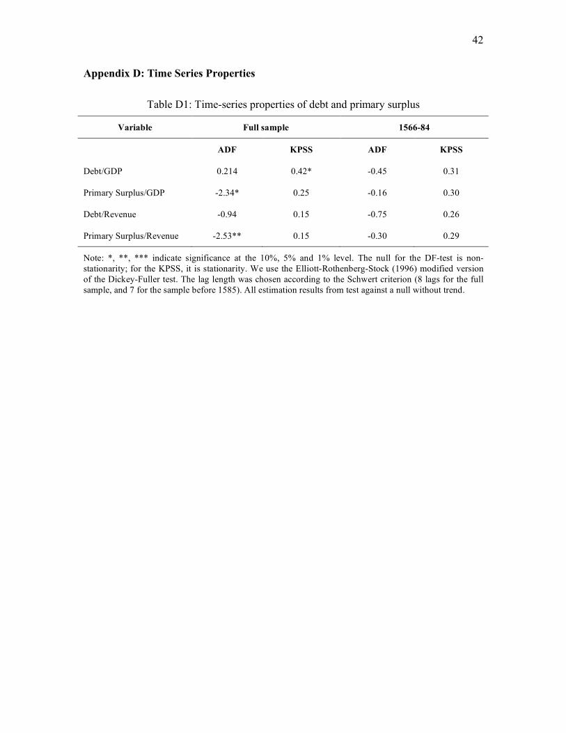
the debt ratio. We perform non-stationarity tests in Appendix D, using both the

Kwiatkowski-Phillips-Schmidt-Shin (1992) test and the Elliott-Rothenberg-Stock (1996)

version of the Augmented Dickey-Fuller test. We find that, in line with our earlier

discussion, the debt/GDP ratio for the whole period appears non-stationary. For the

period up to 1585, we cannot reject the null of either stationarity or of non-stationarity. If

we use the debt to revenue ratio instead, we cannot reject either stationarity or non-

stationarity in the full sample.

The literature on sovereign debt has concluded that non-stationarity tests are a

poor way of examining sustainability, not least because the power of these tests tends to

be low.26 Because of these shortcomings, Bohn (1998) develops an alternative method for

determining sustainability. He estimates fiscal policy functions of the type

ttt dCps !" +•+= (4)

where C is a constant, and ρ indicates the strength of the fiscal reaction to accumulating

debts. Sustainability requires that the primary surplus responds positively to an increase

in debt levels in a linear or more than linear fashion. Our new series for annual primary

surpluses and debt stocks allow us to estimate (4). In contrast to Bohn, we do not attempt

to adjust for temporary expenditure shocks. This is because our sample period is

relatively short, and because Philip II was at war every single year of his reign with the

exception of one. Not adjusting for temporary expenditures shocks biases the coefficient

on debt downwards (Bohn 1998).

Bohn’s period of interest for the US does not include bankruptcies. The haircut

imposed on lenders after a default causes debt to fall, and Bohn’s methodology would 26 Bohn (1998).

27

incorrectly interpret this as a sign of fiscal virtue. To avoid this, in the regressions we use

the debt and primary surplus estimates obtained with the face value approach to

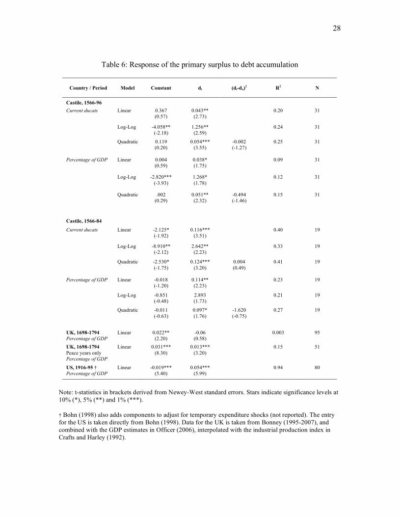
defaults.27 Because of the data concerns surrounding GDP estimates and possible

structural breaks in the series, we estimate three different models (linear, log-log and

quadratic) in four variants each. First, to establish a benchmark, we do not scale the

variables by GDP. We estimate each equation for both the entire sample and, heeding our

findings in the previous exercise, we repeat the analysis for the sub-period 1566-1584.

We then redo the estimations using the data scaled by GDP estimates. Finally, we

estimate linear models using UK data between 1698 and 1794 (both full sample and

peace years only), and we reproduce the estimates for the US from Bohn (1998). All

results are reported in Table 6.

27 See section II above for a discussion of the face value approach to the estimation of debt during defaults.

28

Table 6: Response of the primary surplus to debt accumulation

Country / Period Model Constant dt (dt-da)2 R2 N

Castile, 1566-96

Current ducats Linear 0.367 (0.57)

0.043** (2.73)

0.20 31

Log-Log -4.058** (-2.18)

1.256** (2.59)

0.24 31

Quadratic

0.119 (0.20)

0.054*** (3.55)

-0.002 (-1.27)

0.25 31

Percentage of GDP Linear 0.004 (0.59)

0.038* (1.75)

0.09 31

Log-Log -2.820*** (-3.93)

1.268* (1.78)

0.12 31

Quadratic .002 (0.29)

0.051** (2.32)

-0.494 (-1.46)

0.15 31

Castile, 1566-84

Current ducats Linear -2.125* (-1.92)

0.116*** (3.51)

0.40 19

Log-Log -8.910** (-2.12)

2.642** (2.23)

0.33 19

Quadratic

-2.530* (-1.75)

0.124*** (3.20)

0.004 (0.49)

0.41 19

Percentage of GDP Linear -0.018 (-1.20)

0.114** (2.23)

0.23 19

Log-Log -0.851 (-0.48)

2.893 (1.73)

0.21 19

Quadratic -0.011 (-0.63)

0.097* (1.76)

-1.620 (-0.75)

0.27 19

UK, 1698-1794 Percentage of GDP

Linear 0.022** (2.20)

-0.06 (0.58)

0.003 95

UK, 1698-1794 Peace years only Percentage of GDP

Linear 0.031*** (8.30)

0.013*** (3.20)

0.15 51

US, 1916-95 † Percentage of GDP

Linear -0.019*** (5.40)

0.054*** (5.99)

0.94 80

Note: t-statistics in brackets derived from Newey-West standard errors. Stars indicate significance levels at 10% (*), 5% (**) and 1% (***). † Bohn (1998) also adds components to adjust for temporary expenditure shocks (not reported). The entry for the US is taken directly from Bohn (1998). Data for the UK is taken from Bonney (1995-2007), and combined with the GDP estimates in Officer (2006), interpolated with the industrial production index in Crafts and Harley (1992).

29

In all specifications, we find a strong response of the primary surplus to higher

debt stocks, and the parameters are robust to scaling. In the models covering the entire

period, the coefficient on debt hovers between 0.038 and 0.054, compared with a US

coefficient of 0.054. If the only the sub-period between 1566 and 1584 is considered, the

response almost doubles in strength. This suggests that Habsburg Spain, despite the

strains of constant warfare, reacted with at least as large an increase in her primary

surplus to the accumulation of debt than the US did in the 20th century. There is also no

evidence that fiscal responses slowed down at higher debt levels. In the quadratic

specifications, we only find insignificant coefficients on d2.28 Remarkably, Habsburg

Spain appears to show a much stronger reaction to rising deficits than the UK during the

18th century. Since Great Britain is widely seen as a model of fiscal rectitude in the early

modern era (Brewer 1988; Ferguson 2002), we conclude that the Spanish bankruptcies

did not result from underlying structural weaknesses in fiscal responses.

IV. DISCUSSION AND CONCLUSION

By combining a new series of short-term loans with existing data and a simple

accounting framework, we construct the first comprehensive annual accounts of Spain’s

fiscal position between 1566 and 1596. These series are the earliest of their kind for any

state in history. During this period, the Spanish empire was at the height of its power. The

period also saw the forging of Philip II’s ‘grand strategy,’ the onset of ‘imperial

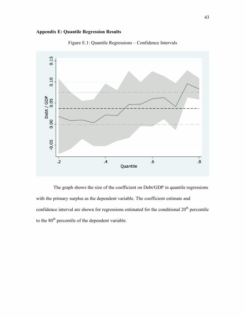
28 In appendix E, we present the results of quantile regressions. These show that the the primary surplus reacted more strongly to more debt at higher levels, offering support for the results from the quadratic specification.

30

overstretch,’ and the unraveling of Spanish hegemony in the wake of military setbacks.29

Overall, Spain’s finances were much healthier than earlier authors allowed. This is

especially true of the years before the “Invincible Armada”. While expenditures rose,

revenues mostly kept pace. Remarkably, Philip II ran a primary surplus in every single

year of his reign, and increased it as debt levels rose. We conclude that Philip’s debt was

sustainable until at least 1584. From this vantage point, the bankruptcy of 1575 appears

as little more than a temporary setback. The suspension of payments seems to have been

triggered by an unforeseen increase in expenditures in the two preceding years. Between

1577 and 1584, the fiscal indicators behaved as they had in earlier decades; the growing

debt was met with an increased primary surplus, and the deficit was kept under control.

The fiscal situation deteriorated in the second half of the 1580s, when Philip

decided to undertake the ‘Enterprise of England.’ The enormous cost of outfitting the

Armada sent the budget deep into the red. The disaster of 1588 and the sudden threat of

British invasion required high levels of military expenditure. The introduction of the

millones and record silver remittances could not rescue the king’s fiscal position. The

outbreak of the Elizabethan war, a direct consequence of the Armada and of Spain’s

involvement in the struggle for the French succession severely undermined Castile’s

finances. Faced with the highest spike in expenditure yet, the Crown had no alternative

but to declare another bankruptcy. By the 1590s, no plausible tax increase would have

been large enough to service the existing debt. Only a prolonged period of peace and

domestic austerity could have rendered the king’s financial position sustainable. Unlike

the 1575 episode, the 1596 suspension was clearly rooted in structural causes.

29 See Kennedy (1987) and Parker (1998).

31

Our sustainability calculations may even be too cautious, as they rely only on

the ex-post outcomes of uncertain events. Ex-ante, it was not clear that Philip II’s strategy

in the Netherlands would fail. Had it succeeded, the vast military expenditures necessary

to subdue the rebels could have been saved. In addition, the rich cities of the Low

Countries would have been taxed heavily. Had the Armada not been destroyed, the

Crown would have saved the expense of building a second fleet, and possibly gained

additional tax revenue. The defeat of 1588 dealt a shattering blow to Spain’s military and

financial position. Hopes of repaying all debts did not founder on the rocks of fiscal

recklessness and ineptitude, as suggested by earlier scholarship. They sank together with

the Armada’s ships in the English Channel.

Our findings suggest that bankers lending to Philip II may ex-ante have been no

less rational than investors in British consols in the early 19th century. At that point,

British government debt stood at more than 200 percent of GDP (Barro 1987). That Spain

would eventually hold the record for serial default, and that Britain would emerge as a

textbook example of fiscal probity, may owe more to success or misfortune on the

battlefield than to fiscal policy itself. In this sense, our results shed additional light on the

nature of serial defaults. Reinhart, Rogoff and Savastano (2003) argue that countries go

bankrupt repeatedly because deeper parameters in their political and social environment

make repayment difficult. Borrowing, for these countries, is unsafe at almost any level.

Default episodes may have important negative knock-on effects on growth and the

quality of fiscal institutions. Sims (2003) points out that even serial defaults may be an

efficient equilibrium outcome, and that there is only limited evidence that bankruptcies

harm fiscal institutions. Spain’s history of 13 defaults between 1500 and 1900 serves a

32

prime example in the work of Reinhart, Rogoff and Savastano (2003). Our results suggest

that Philip’s first suspensions occurred at a time of fiscal probity and reasonable financial

health, and reflected temporary liquidity shortfalls. While it is possible that the

cumulative effect of Philip’s bankruptcies eventually undermined the fiscal and economic

position of Spain, the evidence in our period does not suggest that the quality of fiscal

institutions suffered markedly. If anything, since the king used the defaults as a

negotiating device to raise taxes on the cities, suspensions probably strengthened the tax

powers of the monarch. This implies that it took an accumulation of random shocks –

mostly after the death of Philip II – to eventually lead to serial defaults with negative

economic and institutional consequences.

REFERENCES

Aizenman, Joshua, and Brian Pinto. 2005. Managing Economic Volatility and Crises: A Practitioner's Guide. Cambridge: Cambridge University Press.

Alvarez Nogal, Carlos, and Leandro Prados de la Escosura. 2008. The Decline of Spain (1500-1850): Conjectural Estimates. European Review of Economic History (forthcoming).

Artola, Miguel. 1982. La Hacienda del Antiguo Régimen. Madrid: Alianza. Barro, Robert J. 1987. Government Spending, Interest Rates, Prices, and Budget Deficits

in the United Kingdom, 1701-1918. Journal of Monetary Economics 20 (2):221-247.

Bohn, Henning. 1998. The Behavior of US Public Debt and Deficits. Quarterly Journal of Economics 113 (3):949-963.

Bonney, Richard. 2007. European State Finance Database 1995-2007 [cited August 23 2007]. Available from http://www.le.ac.uk/hi/bon/ESFDB/.

———. 1999. The Rise of the Fiscal State in Europe, c. 1200-1815. Oxford: Oxford University Press.

Braudel, Fernand. 1966. The Mediterranean and the Mediterranean World in the Age of Philip II. Second Revised Edition ed. Glasgow: William Colins & Sons.

Brewer, John S. 1988. The Sinews of Power. Cambridge: Harvard University Press. Bulow, Jeremy, and Kenneth Rogoff. 1989. A Constant Recontracting Model of

Sovereign Debt. Journal of Political Economy 97 1:155-78. Carande, Ramón. 1987. Carlos V y sus banqueros. 3. ed. 3 vols. Barcelona: Crítica.

33

Carreras, Albert. 2003. Modern Spain. In The Oxford Encyclopedia of Economic History, edited by J. Mokyr. New York: Oxford University Press.

Celasu, OYa, Xavier Debrun, and Jonathan Ostry. 2007. Primary Surplus Behavior and Risks to Fiscal Sustainability in Emerging Market Countries: A "Fan-Chart" Approach. IMF Staff Papers 53 (3).

Conklin, James. 1998. The Theory of Sovereign Debt and Spain under Philip II. Journal of Political Economy 106 3:483-513.

Crafts, N. F. R., and C. Knick Harley. 1992. Output Growth and the British Industrial Revolution: A Restatement of the Crafts-Harley View. Economic History Review 45:703-730.

Dickson, P. G. M. 1967. The Financial Revolution in England. A Study in the Development of Public Credit. London: Macmillan.

Drelichman, Mauricio, and Hans-Joachim Voth. 2008. Institutions and the Resource Curse in Early Modern Spain. In Institutions and Economic Performance, edited by E. Helpman. Cambridge: Harvard University Press.

Elliott, G., T. Rothenberg, and J. H. Stock. 1996. Efficient Tests for an Autoregressive Unit Root. Econometrica 64:813-836.

Ferguson, Niall. 2002. The Cash Nexus: Money and Power in the Modern World, 1700-2000. New York: Basic Books.

Gelabert, Juan. 1999. Castile, 1504-1808. In The Rise of the Fiscal State in Europe, c. 1200-1815, edited by R. Bonney. Oxford: Oxford University Press.

Hamilton, Earl J. 1934. American Treasure and the Price Revolution in Spain, 1501-1650. Cambridge: Harvard University Press.

Hoffman, Philip T., and Kathryn Norberg. 1994. Fiscal Crises, Liberty, and Representative Government, 1450-1789. Stanford: Stanford University Press.

Homer, Sydney, and Richard Sylla. 2005. A History of Interest Rates. Fourth ed. Hoboken: John Wiley & Sons.

IMF. 2003. World Economic Outlook. Washington: IMF. Jago, Charles. 1985. Philip II and the Cortes of Castile: The Case of the Cortes of 1576.

Past and Present 109:22-43. Kennedy, Paul M. 1987. The rise and fall of the great powers : economic change and

military conflict from 1500 to 2000. New York, NY: Random House. Kwiatkowski, Denis, Peter C. B. Phillips, Peter Schmidt, and Yongcheol Shin. 1992.

Testing the null hypothesis of stationarity against the alternative of a unit root : How sure are we that economic time series have a unit root? Journal of Econometrics 54:159-178.

Lovett, A. W. 1980. The Castilian Bankruptcy of 1575. The Historical Journal 23:899-911.

———. 1982. The General Settlement of 1577: An Aspect of Spanish Finance in the Early Modern Period. The Historical Journal 25 (1):1-22.

Marcos Martín, Alberto. 2000. España en los siglos XVI, XVII y XVIII. Barcelona: Crítica.

Neri, Erica. 1989. Uomini d'affari e di governo tra Genova e Madrid. Milano: Vita e Pensiero - Pubblicazioni dell'Università Cattolica.

Officer, Lawrence. 2006. The Annual Real and Nominal GDP for the United Kingdom, 1086-2005: Economic History Services.

34

Ormrod, W. M., Richard Bonney, and Margaret Bonney. 1999. Crises, Revolutions, and Self-Sustained Growth. Essays in European Fiscal History. Stamford: SHAUN TYAS.

Parker, Geoffrey. 1998. The Grand Strategy of Philip II. New Haven and London: Yale University Press.

Reinhart, Carmen M., Kenneth S. Rogoff, and Miguel A. Savastano. 2003. Debt Intolerance. Brookings Papers on Economic Activity 2003 (1):1-74.

Ruiz Martín, Felip. 1965. Un expediente financiero entre 1560 y 1575. La hacienda de Felipe II y la Casa de Contratación de Sevilla. Moneda y Crédito 92:3-58.

Ruiz Martín, Felipe. 1968. Las finanzas españolas durante el reinado de Felipe II. Cuadernos de Historia, Anexos de la Revista Hispania 2:181-203.

Sims, Chris. 2003. Comments on 'Debt Intolerance". Brookings Papers on Economic Activity 2003v (1):63-74.

Thompson, I. A. A. 1976. War and Government in Habsburg Spain. London: The Athlone Press - University of London.

———. 1994. Castile: Polity, Fiscality, and Fiscal Crisis. In Fiscal Crises, Liberty, and Representative Government, 1450-1789, edited by P. T. Hoffman and K. Norberg. Stanford: Stanford University Press.

Toboso Sánchez, Pilar. 1987. La deuda pública castellana durante el Antiguo Régimen (juros) y su liquidación en el siglo XIX. Madrid: Instituto de Estudios Fiscales.

Tortella, Gabriel, and Francisco Comín. 2001. Fiscal and monetary institutions in Spain (1600-1900). In Transferring Wealth and Power from the Old World to the New. Monetary and Fiscal Institutions in the 17th through the 19th Centuries., edited by M. D. Bordo and R. Cortés Conde. Cambridge: Cambridge University Press.

Ulloa, Modesto. 1977. La hacienda real de Castilla en el reinado de Felipe II. [2. ed. Madrid: Fundación Universitaria Española, Seminario Cisneros.

Yun Casalilla, Bartolomé. 2002. El Siglo de la Hegemonía Castellana (1450-1590). In Historia Económica de España, Siglos X-XX, edited by F. Comín, M. Hernández and E. Llopis. Barcelona: Crítica.

———. 2004. Marte contra Minerva. El precio del imperio español, c. 1450-1600. Barcelona: Crítica.

35

Appendix A: Data and estimates

Table A1: Revenues by Type, 1555-1596 (millions of ducats)

Year Sales tax

Customs (internal and

external) Monopolies Direct

taxes Millones Church revenues Confiscation Indies Total

1555 0.933 0.513 0.399 0.432 0.000 0.411 0.000 0.372 3.061 1556 0.933 0.513 0.405 0.404 0.000 0.411 0.000 0.704 3.369 1557 0.939 0.500 0.404 0.404 0.000 0.411 0.000 0.425 3.083 1558 0.939 0.497 0.404 0.404 0.000 0.307 0.000 0.644 3.195 1559 0.939 0.490 0.330 0.404 0.000 0.360 0.000 0.000 2.523

1560 0.939 0.515 0.331 0.404 0.000 0.360 0.034 0.573 3.155 1561 0.939 0.585 0.375 0.565 0.000 0.530 0.000 0.704 3.698 1562 1.277 0.690 0.440 0.537 0.000 0.531 0.000 0.199 3.674 1563 1.277 0.720 0.483 0.537 0.000 0.533 0.000 0.455 4.005 1564 1.277 0.737 0.542 0.404 0.000 0.807 0.000 0.474 4.241 1565 1.277 0.781 0.575 0.404 0.000 0.807 0.000 0.352 4.197

1566 1.277 0.791 0.532 0.404 0.000 0.807 0.000 0.921 4.732 1567 1.277 1.076 0.501 0.432 0.000 0.554 0.202 0.368 4.411 1568 1.277 1.132 0.505 0.404 0.000 0.522 0.427 1.210 5.477 1569 1.277 1.136 0.484 0.404 0.000 0.360 0.260 0.949 4.870 1570 1.277 1.064 0.520 0.537 0.000 0.554 0.079 1.010 5.041 1571 1.277 1.115 0.537 0.537 0.000 0.597 0.008 1.068 5.139

1572 1.277 1.083 0.527 0.537 0.000 1.200 0.554 0.605 5.782 1573 1.277 1.090 0.549 0.432 0.000 1.200 0.181 0.708 5.437 1574 1.277 0.985 0.587 0.404 0.000 1.316 0.411 0.700 5.680 1575 3.091 0.975 0.616 0.404 0.000 1.018 0.619 0.917 7.639 1576 3.715 0.978 0.579 0.404 0.000 1.260 0.135 0.988 8.059 1577 3.715 1.000 0.583 0.404 0.000 1.233 0.040 2.168 9.143

1578 2.715 0.994 0.661 0.404 0.000 1.431 0.301 1.448 7.953 1579 2.715 1.006 0.652 0.444 0.000 1.290 0.025 1.437 7.568 1580 2.715 0.992 0.636 0.404 0.000 1.286 0.042 1.739 7.813 1581 2.715 0.983 0.592 0.404 0.000 0.933 0.000 1.737 7.364 1582 2.715 0.994 0.442 0.404 0.000 1.336 0.049 0.498 6.437 1583 2.715 1.014 0.472 0.404 0.000 1.274 0.000 3.200 9.078

1584 2.715 1.037 0.472 0.404 0.000 1.299 0.067 1.857 7.850 1585 2.715 1.018 0.472 0.439 0.000 1.310 0.359 2.226 8.539 1586 2.715 1.038 0.533 0.404 0.000 1.314 0.350 0.890 7.243 1587 2.715 1.028 0.524 0.404 0.000 1.432 0.382 4.472 10.957 1588 2.755 0.993 0.595 0.404 0.000 1.211 0.281 1.519 7.757 1589 2.755 0.999 0.529 0.404 0.000 1.338 0.356 2.322 8.703

1590 2.755 1.020 0.869 0.404 0.000 1.384 0.202 1.836 8.469 1591 2.755 1.033 0.896 0.444 1.338 1.378 0.788 0.697 9.329 1592 2.755 0.974 0.825 0.404 1.338 1.380 0.000 2.985 10.660 1593 2.755 1.008 0.912 0.404 1.338 1.283 0.592 2.089 10.381 1594 2.755 1.015 0.816 0.404 1.338 1.438 0.230 0.000 7.996 1595 2.755 1.017 1.010 0.404 1.333 1.476 0.325 5.738 14.058

1596 2.755 1.026 0.784 0.404 1.333 1.501 0.108 3.418 11.328

36

Table A2: Asientos

Year Ducats Year Ducats

1520 4,454 1566 1,308,635 1521 55,834 1567 6,465,559 1522 156,502 1568 1,427,573 1523 348,103 1569 2,862,427 1524 60,858 1570 1,957,884 1525 172,415 1571 3,691,306 1526 358,224 1572 5,853,273 1527 472,917 1573 2,636,034 1528 599,668 1574 6,177,371 1529 794,567 1575 5,472,220 1530 830,467 1576 106,666 1531 904,406 1577 0 1532 620,638 1578 263,325 1533 5,225 1579 0 1534 222,473 1580 760,480 1535 764,733 1581 195,466 1536 981,600 1582 3,358,708 1537 970,004 1583 539,529 1538 830,655 1584 640,000 1539 842,334 1585 0 1540 366,100 1586 2,072,763 1541 110,609 1587 5,327,485 1542 343,936 1588 2,660,480 1543 1,742,301 1589 5,241,068 1544 1,424,778 1590 5,120,747 1545 353,182 1591 4,408,931 1546 1,708,020 1592 655,505 1547 451,026 1593 3,354,716 1548 484,811 1594 6,052,300 1549 147,370 1595 6,880,807 1550 615,933 1596 3,074,943 1551 1,470,195 1597 582,265 1552 3,595,147 1598 0 1553 2,271,108 1599 1,734,471 1554 1,258,368 1600 5,056,161 1555 1,091,813 1556 1,427,433

37

Table A3: Estimates of outstanding debt (millions of ducats)30

Year

(1)

Ulloa

FV

(2)

Ulloa

MV

(3)

Our series

FV

(4)

Our series

MV

(5)

Max series

FV

(6)

Max series

MV

1565 25.000 25.000 25.000 25.000 25.000 25.000 1566 25.654 25.654 25.380 25.380 25.630 25.630 1567 27.511 27.511 27.259 27.259 27.421 27.421 1568 27.845 27.845 27.674 27.674 27.799 27.799 1569 28.664 28.664 28.506 28.506 28.589 28.589 1570 29.213 29.213 29.075 29.075 29.118 29.118 1571 29.976 29.976 30.148 30.148 30.094 30.094 1572 31.796 31.796 31.849 31.849 31.850 31.850 1573 32.896 32.896 32.615 32.615 32.910 32.910 1574 34.599 34.599 34.410 34.410 34.553 34.553 1575 40.644 40.644 40.644 40.644 40.644 40.644 1576 40.644 40.644 40.644 40.644 40.644 40.644 1577 38.440 35.106 38.440 35.106 38.440 35.106 1578 38.654 35.355 38.592 35.283 38.646 35.346 1579 38.654 35.355 38.592 35.283 38.646 35.346 1580 38.918 35.662 39.031 35.793 39.015 35.775 1581 39.364 36.180 39.143 35.924 39.445 36.275 1582 41.587 38.765 41.082 38.178 41.592 38.770 1583 42.079 39.336 41.394 38.539 42.066 39.321 1584 42.079 39.336 41.763 38.969 42.376 39.682 1585 42.603 39.945 41.763 38.969 42.882 40.270 1586 43.371 40.838 42.959 40.360 43.887 41.437 1587 46.164 44.084 46.034 43.934 46.583 44.571 1588 47.164 45.247 47.570 45.719 47.872 46.070 1589 50.065 48.618 50.595 49.235 50.672 49.325 1590 52.853 51.859 53.551 52.671 53.364 52.453 1591 55.332 54.740 56.096 55.629 55.757 55.235 1592 55.967 55.479 56.474 56.068 56.371 55.948 1593 58.039 57.887 58.411 58.319 58.371 58.273 1594 61.145 61.498 61.904 62.380 61.370 61.759 1595 65.982 67.119 65.876 66.996 66.040 67.186 1596 67.651 69.059 67.651 69.059 67.651 69.059 1597 68.000 68.000 68.000 68.000 68.000 68.000 1598 68.000 68.000 68.000 68.000 68.000 68.000 1599 68.871 69.012 69.001 69.164 68.840 68.977 1600 71.408 71.962 71.920 72.556 71.291 71.825

30 It bears repeating that “face value” and “market value,” represented by the letters FV and MV in the table, do not refer to the valuation of outstanding debt, but rather to the methodology for computing the size of the haircut in each default.

38

Table A4: Fiscal position

Year

(1) Revenues

(2) Ordinary

expenditure

(3)=(1)-(2)=(4)-(6) Primary surplus

(4) Debt

service

(5)=(2)+(4) Total

expenditure

(6)=(1)-(5) Deficit

1566 4.732 2.641 2.092 2.472 5.113 0.380 1567 4.411 3.702 0.709 2.587 6.290 1.879 1568 5.477 3.334 2.143 2.558 5.892 0.415 1569 4.870 3.137 1.733 2.565 5.702 0.832 1570 5.041 3.066 1.975 2.544 5.610 0.569 1571 5.139 3.648 1.490 2.563 6.211 1.073 1572 5.782 4.854 0.928 2.629 7.483 1.701 1573 5.437 3.592 1.845 2.611 6.203 0.766 1574 5.680 4.806 0.875 2.670 7.476 1.795 1575 7.639 6.674 0.965 3.053 9.726 2.088 1576 8.059 6.674 1.385 0.000 6.674 -1.385 1577 9.143 6.674 2.469 2.463 9.137 -0.006 1578 7.953 5.742 2.211 2.388 8.130 0.177 1579 7.568 5.268 2.301 2.301 7.568 0.000 1580 7.813 6.078 1.735 2.245 8.323 0.510 1581 7.364 5.138 2.226 2.357 7.495 0.131 1582 6.437 6.075 0.362 2.615 8.690 2.253 1583 9.078 6.689 2.389 2.751 9.440 0.362 1584 7.850 5.385 2.465 2.894 8.279 0.429 1585 8.539 5.533 3.006 3.006 8.539 0.000 1586 7.243 5.403 1.839 3.230 8.633 1.391 1587 10.957 10.889 0.069 3.643 14.531 3.574 1588 7.757 5.619 2.138 3.923 9.542 1.785 1589 8.703 7.853 0.850 4.367 12.219 3.516 1590 8.469 7.081 1.388 4.823 11.905 3.436 1591 9.329 7.033 2.296 5.254 12.287 2.958 1592 10.660 5.642 5.018 5.458 11.099 0.440 1593 10.381 6.786 3.594 5.845 12.631 2.251 1594 7.996 5.624 2.371 6.432 12.056 4.061 1595 14.058 11.573 2.485 7.101 18.674 4.616 1596 11.328 5.872 5.456 7.519 13.391 2.063

39

Appendix B: Comparing the new revenue series with existing estimates

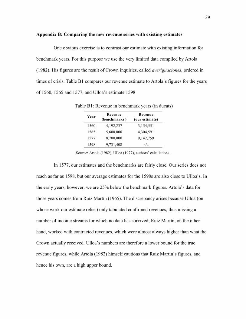
One obvious exercise is to contrast our estimate with existing information for

benchmark years. For this purpose we use the very limited data compiled by Artola

(1982). His figures are the result of Crown inquiries, called averiguaciones, ordered in

times of crisis. Table B1 compares our revenue estimate to Artola’s figures for the years

of 1560, 1565 and 1577, and Ulloa’s estimate 1598

Table B1: Revenue in benchmark years (in ducats)

Year Revenue (benchmarks )

Revenue (our estimate)

1560 4,192,237 3,154,551 1565 5,600,000 4,304,591 1577 8,700,000 9,142,759 1598 9,731,408 n/a

Source: Artola (1982), Ulloa (1977), authors’ calculations.

In 1577, our estimates and the benchmarks are fairly close. Our series does not

reach as far as 1598, but our average estimates for the 1590s are also close to Ulloa’s. In

the early years, however, we are 25% below the benchmark figures. Artola’s data for

those years comes from Ruíz Martín (1965). The discrepancy arises because Ulloa (on

whose work our estimate relies) only tabulated confirmed revenues, thus missing a

number of income streams for which no data has survived; Ruíz Martín, on the other

hand, worked with contracted revenues, which were almost always higher than what the

Crown actually received. Ulloa’s numbers are therefore a lower bound for the true

revenue figures, while Artola (1982) himself cautions that Ruiz Martín’s figures, and

hence his own, are a high upper bound.

40

Appendix C: the Medios Generales of 1577 and 1597

The medio general of 1577 settled the suspension of payments of September 1,

1575. This account is taken directly from the original document subscribed by the king

and the bankers, preserved in the Archive of Simancas. Its location is Asiento y Medio

General de la Hacienda. Archivo General de Simancas; Consejo y Juntas de Hacienda;

Libro 42.

The king recognized outstanding obligations for 15,184,464 ducats, divided

14,600,446 ducats of outstanding principal as of September 1, 1575, and 584,018 ducats

in interest accrued between September 1 and December 1, 1575. It is not clear why this

interest was added; in any event, the first provision of the settlement was to write it off.

We work from the outstanding capital at the time of the suspension, 14.6 million ducats.

Of the total outstanding asientos, 5,580,313 ducats were collateralized by

perpetual juros with a yield of 7.14% guaranteed by ordinary revenues. The holders of

these juros were allowed to keep them, but their annuity rate was reduced to 5%.

Assuming 7.14% represented the market interest rate a banker could obtain, the reduction

in the annuity rate amounts to a write-off of 1,672,531 ducats.

A further 4,375,994 ducats worth of asientos were collateralized by perpetual

juros with a yield of 5% guaranteed by the revenues of the Casa de la Contratación. The

Casa had been a poster boy of inefficient administration and these juros were often not

serviced; in the secondary market they traded at around 50% of their face value. The

Crown recognized 55% of juros de contratación at face value by converting them to 5%

perpetuities guaranteed by ordinary revenues. The remainder 45%, 1,969,197 ducats’

worth, were considered uncollateralized debt.

41

Uncollateralized debt, which amounted to 6,613,336 ducats including the juros

de contratación, suffered the harshest treatment. Two thirds of it was converted into

perpetuities of the same face value yielding 3.3%. The remainder third was converted

into tax farms on small towns (vasallos) with a nominal yield of 2.3%. The write-off on

this portion of the debt relative to a 7.14% market rate amounts to 3,865,498 ducats.

In total, the 1575 medio general rescheduled a total of 14,600,446 ducats of short term

debt, on which it imposed a haircut of 5,538,029 ducats, or 37.93% of the loans in

default.

The 1596 bankruptcy, which we describe following Ulloa (1977, p. 823) and

Erica Neri (1989, p. 109), was mild in comparison. The 1597 settlement rescheduled a

total 7,048,000 ducats. Two thirds, or 4,698,667 ducats’ worth, were converted into 5%

perpetual juros. Using the same market rate assumption as for the 1575 settlement, this

would imply a haircut of 1,408,284 ducats. The remaining third was guaranteed by 12.5%

lifetime juros in possession of the bankers; these lifetime bonds had been issued in 1580,

and hence were halfway through their accounting life expectancy of 33 years. The

settlement stipulated that they were to be swapped by 7.14% perpetual juros; the bankers

would be given enough perpetual juros so as not to alter the present value of the

principal. In short, this portion of the outstanding debt suffered no write off; the king

lengthened the repayment schedule at the cost of increasing the face value of the bonds.

The total write-off of the 1597 settlement was therefore 1,408,284 ducats, or 19.98% of

the amount defaulted upon.

42

Appendix D: Time Series Properties

Table D1: Time-series properties of debt and primary surplus

Variable Full sample 1566-84

ADF KPSS ADF KPSS

Debt/GDP 0.214 0.42* -0.45 0.31

Primary Surplus/GDP -2.34* 0.25 -0.16 0.30

Debt/Revenue -0.94 0.15 -0.75 0.26

Primary Surplus/Revenue -2.53** 0.15 -0.30 0.29

Note: *, **, *** indicate significance at the 10%, 5% and 1% level. The null for the DF-test is non-stationarity; for the KPSS, it is stationarity. We use the Elliott-Rothenberg-Stock (1996) modified version of the Dickey-Fuller test. The lag length was chosen according to the Schwert criterion (8 lags for the full sample, and 7 for the sample before 1585). All estimation results from test against a null without trend.

43

Appendix E: Quantile Regression Results

Figure E.1: Quantile Regressions – Confidence Intervals

The graph shows the size of the coefficient on Debt/GDP in quantile regressions

with the primary surplus as the dependent variable. The coefficient estimate and

confidence interval are shown for regressions estimated for the conditional 20th percentile

to the 80th percentile of the dependent variable.