Embed Size (px)
Citation preview

SAS/STAT® 13.1 User’s GuideThe SURVEYFREQProcedure

This document is an individual chapter from SAS/STAT® 13.1 User’s Guide.
The correct bibliographic citation for the complete manual is as follows: SAS Institute Inc. 2013. SAS/STAT® 13.1 User’s Guide.Cary, NC: SAS Institute Inc.
Copyright © 2013, SAS Institute Inc., Cary, NC, USA
All rights reserved. Produced in the United States of America.
For a hard-copy book: No part of this publication may be reproduced, stored in a retrieval system, or transmitted, in any form or byany means, electronic, mechanical, photocopying, or otherwise, without the prior written permission of the publisher, SAS InstituteInc.
For a web download or e-book: Your use of this publication shall be governed by the terms established by the vendor at the timeyou acquire this publication.
The scanning, uploading, and distribution of this book via the Internet or any other means without the permission of the publisher isillegal and punishable by law. Please purchase only authorized electronic editions and do not participate in or encourage electronicpiracy of copyrighted materials. Your support of others’ rights is appreciated.
U.S. Government License Rights; Restricted Rights: The Software and its documentation is commercial computer softwaredeveloped at private expense and is provided with RESTRICTED RIGHTS to the United States Government. Use, duplication ordisclosure of the Software by the United States Government is subject to the license terms of this Agreement pursuant to, asapplicable, FAR 12.212, DFAR 227.7202-1(a), DFAR 227.7202-3(a) and DFAR 227.7202-4 and, to the extent required under U.S.federal law, the minimum restricted rights as set out in FAR 52.227-19 (DEC 2007). If FAR 52.227-19 is applicable, this provisionserves as notice under clause (c) thereof and no other notice is required to be affixed to the Software or documentation. TheGovernment’s rights in Software and documentation shall be only those set forth in this Agreement.
SAS Institute Inc., SAS Campus Drive, Cary, North Carolina 27513-2414.
December 2013
SAS provides a complete selection of books and electronic products to help customers use SAS® software to its fullest potential. Formore information about our offerings, visit support.sas.com/bookstore or call 1-800-727-3228.
SAS® and all other SAS Institute Inc. product or service names are registered trademarks or trademarks of SAS Institute Inc. in theUSA and other countries. ® indicates USA registration.
Other brand and product names are trademarks of their respective companies.

SAS and all other SAS Institute Inc. product or service names are registered trademarks or trademarks of SAS Institute Inc. in the USA and other countries. ® indicates USA registration. Other brand and product names are trademarks of their respective companies. © 2013 SAS Institute Inc. All rights reserved. S107969US.0613
Discover all that you need on your journey to knowledge and empowerment.
support.sas.com/bookstorefor additional books and resources.
Gain Greater Insight into Your SAS® Software with SAS Books.


Chapter 94
The SURVEYFREQ Procedure
ContentsOverview: SURVEYFREQ Procedure . . . . . . . . . . . . . . . . . . . . . . . . . . . . . 7990Getting Started: SURVEYFREQ Procedure . . . . . . . . . . . . . . . . . . . . . . . . . . 7990Syntax: SURVEYFREQ Procedure . . . . . . . . . . . . . . . . . . . . . . . . . . . . . . 7999
PROC SURVEYFREQ Statement . . . . . . . . . . . . . . . . . . . . . . . . . . . . 8000BY Statement . . . . . . . . . . . . . . . . . . . . . . . . . . . . . . . . . . . . . . 8007CLUSTER Statement . . . . . . . . . . . . . . . . . . . . . . . . . . . . . . . . . . 8008REPWEIGHTS Statement . . . . . . . . . . . . . . . . . . . . . . . . . . . . . . . . 8008STRATA Statement . . . . . . . . . . . . . . . . . . . . . . . . . . . . . . . . . . . 8010TABLES Statement . . . . . . . . . . . . . . . . . . . . . . . . . . . . . . . . . . . 8010WEIGHT Statement . . . . . . . . . . . . . . . . . . . . . . . . . . . . . . . . . . . 8030
Details: SURVEYFREQ Procedure . . . . . . . . . . . . . . . . . . . . . . . . . . . . . . 8031Specifying the Sample Design . . . . . . . . . . . . . . . . . . . . . . . . . . . . . . 8031Domain Analysis . . . . . . . . . . . . . . . . . . . . . . . . . . . . . . . . . . . . . 8033Missing Values . . . . . . . . . . . . . . . . . . . . . . . . . . . . . . . . . . . . . . 8033Statistical Computations . . . . . . . . . . . . . . . . . . . . . . . . . . . . . . . . . 8036
Variance Estimation . . . . . . . . . . . . . . . . . . . . . . . . . . . . . . . 8036Definitions and Notation . . . . . . . . . . . . . . . . . . . . . . . . . . . . 8037Totals . . . . . . . . . . . . . . . . . . . . . . . . . . . . . . . . . . . . . . 8038Covariance of Totals . . . . . . . . . . . . . . . . . . . . . . . . . . . . . . 8040Proportions . . . . . . . . . . . . . . . . . . . . . . . . . . . . . . . . . . . 8040Row and Column Proportions . . . . . . . . . . . . . . . . . . . . . . . . . 8042Balanced Repeated Replication (BRR) . . . . . . . . . . . . . . . . . . . . . 8043The Jackknife Method . . . . . . . . . . . . . . . . . . . . . . . . . . . . . 8046Confidence Limits for Totals . . . . . . . . . . . . . . . . . . . . . . . . . . 8048Confidence Limits for Proportions . . . . . . . . . . . . . . . . . . . . . . . 8048Degrees of Freedom . . . . . . . . . . . . . . . . . . . . . . . . . . . . . . 8051Coefficient of Variation . . . . . . . . . . . . . . . . . . . . . . . . . . . . . 8052Design Effect . . . . . . . . . . . . . . . . . . . . . . . . . . . . . . . . . . 8052Expected Weighted Frequency . . . . . . . . . . . . . . . . . . . . . . . . . 8053Risks and Risk Difference . . . . . . . . . . . . . . . . . . . . . . . . . . . 8054Odds Ratio and Relative Risks . . . . . . . . . . . . . . . . . . . . . . . . . 8055Kappa Coefficients . . . . . . . . . . . . . . . . . . . . . . . . . . . . . . . 8057Rao-Scott Chi-Square Test . . . . . . . . . . . . . . . . . . . . . . . . . . . 8060Rao-Scott Likelihood Ratio Chi-Square Test . . . . . . . . . . . . . . . . . . 8065Wald Chi-Square Test . . . . . . . . . . . . . . . . . . . . . . . . . . . . . . 8067Wald Log-Linear Chi-Square Test . . . . . . . . . . . . . . . . . . . . . . . 8068

7990 F Chapter 94: The SURVEYFREQ Procedure
Output Data Sets . . . . . . . . . . . . . . . . . . . . . . . . . . . . . . . . . . . . . 8069Displayed Output . . . . . . . . . . . . . . . . . . . . . . . . . . . . . . . . . . . . . 8070ODS Table Names . . . . . . . . . . . . . . . . . . . . . . . . . . . . . . . . . . . . 8077ODS Graphics . . . . . . . . . . . . . . . . . . . . . . . . . . . . . . . . . . . . . . 8078
Examples: SURVEYFREQ Procedure . . . . . . . . . . . . . . . . . . . . . . . . . . . . . 8078Example 94.1: Two-Way Tables . . . . . . . . . . . . . . . . . . . . . . . . . . . . . 8078Example 94.2: Multiway Tables (Domain Analysis) . . . . . . . . . . . . . . . . . . 8082Example 94.3: Output Data Sets . . . . . . . . . . . . . . . . . . . . . . . . . . . . 8084
References . . . . . . . . . . . . . . . . . . . . . . . . . . . . . . . . . . . . . . . . . . . 8085
Overview: SURVEYFREQ ProcedureThe SURVEYFREQ procedure produces one-way to n-way frequency and crosstabulation tables from samplesurvey data. These tables include estimates of population totals, population proportions, and their standarderrors. Confidence limits, coefficients of variation, and design effects are also available. The procedureprovides a variety of options to customize the table display.
For one-way frequency tables, PROC SURVEYFREQ provides Rao-Scott chi-square goodness-of-fit tests,which are adjusted for the sample design. You can test a null hypothesis of equal proportions for a one-wayfrequency table, or you can input custom nu5ll hypothesis proportions for the test. For two-way tables,PROC SURVEYFREQ provides design-adjusted tests of independence, or no association, between the rowand column variables. These tests include the Rao-Scott chi-square test, the Rao-Scott likelihood ratio test,the Wald chi-square test, and the Wald log-linear chi-square test. For 2 � 2 tables, PROC SURVEYFREQcomputes estimates and confidence limits for risks (row proportions), the risk difference, the odds ratio, andrelative risks.
PROC SURVEYFREQ computes variance estimates based on the sample design used to obtain the surveydata. The design can be a complex multistage survey design with stratification, clustering, and unequalweighting. PROC SURVEYFREQ provides a choice of variance estimation methods, which include Taylorseries linearization, balanced repeated replication (BRR), and the jackknife.
PROC SURVEYFREQ uses ODS Graphics to create graphs as part of its output. For general informationabout ODS Graphics, see Chapter 21, “Statistical Graphics Using ODS.” For specific information about thestatistical graphics available with the SURVEYFREQ procedure, see the PLOTS= option in the TABLESstatement and the section “ODS Graphics” on page 8078.
Getting Started: SURVEYFREQ ProcedureThe following example shows how you can use PROC SURVEYFREQ to analyze sample survey data. Theexample uses data from a customer satisfaction survey for a student information system (SIS), which is asoftware product that provides modules for student registration, class scheduling, attendance, grade reporting,and other functions.

Getting Started: SURVEYFREQ Procedure F 7991
The software company conducted a survey of school personnel who use the SIS. A probability sample of SISusers was selected from the study population, which included SIS users at middle schools and high schoolsin the three-state area of Georgia, South Carolina, and North Carolina. The sample design for this surveywas a two-stage stratified design. A first-stage sample of schools was selected from the list of schools in thethree-state area that use the SIS. The list of schools (the first-stage sampling frame) was stratified by stateand by customer status (whether the school was a new user of the system or a renewal user). Within thefirst-stage strata, schools were selected with probability proportional to size and with replacement, wherethe size measure was school enrollment. From each sample school, five staff members were randomlyselected to complete the SIS satisfaction questionnaire. These staff members included three teachers and twoadministrators or guidance department members.
The SAS data set SIS_Survey contains the survey results, as well as the sample design information needed toanalyze the data. This data set includes an observation for each school staff member responding to the survey.The variable Response contains the staff member’s response about overall satisfaction with the system.
The variable State contains the school’s state, and the variable NewUser contains the school’s customerstatus (‘New Customer’ or ‘Renewal Customer’). These two variables determine the first-stage strata fromwhich schools were selected. The variable School contains the school identification code and identifies thefirst-stage sampling units (clusters). The variable SamplingWeight contains the overall sampling weight foreach respondent. Overall sampling weights were computed from the selection probabilities at each stage ofsampling and were adjusted for nonresponse.
Other variables in the data set SIS_Survey include SchoolType and Department. The variable SchoolTypeidentifies the school as a high school or a middle school. The variable Department identifies the staff memberas a teacher, or an administrator or guidance department member.
The following PROC SURVEYFREQ statements request a one-way frequency table for the variableResponse:
title 'Student Information System Survey';proc surveyfreq data=SIS_Survey;
tables Response;strata State NewUser;cluster School;weight SamplingWeight;
run;
The PROC SURVEYFREQ statement invokes the procedure and identifies the input data set to be analyzed.The TABLES statement requests a one-way frequency table for the variable Response. The table requestsyntax for PROC SURVEYFREQ is very similar to the table request syntax for PROC FREQ. This exampleshows a request for a single one-way table, but you can also request two-way tables and multiway tables.As in PROC FREQ, you can request more than one table in the same TABLES statement, and you can usemultiple TABLES statements in the same invocation of the procedure.
The STRATA, CLUSTER, and WEIGHT statements provide sample design information for the procedure,so that the analysis is done according to the sample design used for the survey, and the estimates apply tothe study population. The STRATA statement names the variables State and NewUser, which identify thefirst-stage strata. Note that the design for this example also includes stratification at the second stage ofselection (by type of school personnel), but you specify only the first-stage strata for PROC SURVEYFREQ.The CLUSTER statement names the variable School, which identifies the clusters (primary sampling units).The WEIGHT statement names the sampling weight variable.

7992 F Chapter 94: The SURVEYFREQ Procedure
Figure 94.1 and Figure 94.2 display the output produced by PROC SURVEYFREQ, which includes the “DataSummary” table and the one-way table, “Table of Response.” The “Data Summary” table is produced bydefault unless you specify the NOSUMMARY option. This table shows there are 6 strata, 370 clusters orschools, and 1850 observations (respondents) in the SIS_Survey data set. The sum of the sampling weightsis approximately 39,000, which estimates the total number of school personnel in the study area that use theSIS.
Figure 94.1 SIS_Survey Data Summary
Student Information System Survey
The SURVEYFREQ Procedure
Data Summary
Number of Strata 6Number of Clusters 370Number of Observations 1850Sum of Weights 38899.6482
Figure 94.2 displays the one-way table of Response, which provides estimates of the population total(weighted frequency) and the population percentage for each category (level) of the variable Response. Theresponse level ‘Very Unsatisfied’ has a frequency of 304, which means that 304 sample respondents fallinto this category. It is estimated that 17.17% of all school personnel in the study population fall into thiscategory, and the standard error of this estimate is 1.29%. Note that the estimates apply to the population ofall SIS users in the study area, as opposed to describing only the sample of 1850 respondents. The estimateof the total number of school personnel that are ‘Very Unsatisfied’ is 6,678, with a standard deviation of 502.The standard errors computed by PROC SURVEYFREQ are based on the multistage stratified design of thesurvey. This differs from some of the traditional analysis procedures, which assume the design is simplerandom sampling from an infinite population.
Figure 94.2 One-Way Table of Response
Table of Response
Weighted Std Dev of Std Err ofResponse Frequency Frequency Wgt Freq Percent Percent------------------------------------------------------------------------------Very Unsatisfied 304 6678 501.61039 17.1676 1.2872Unsatisfied 326 6907 495.94101 17.7564 1.2712Neutral 581 12291 617.20147 31.5965 1.5795Satisfied 455 9309 572.27868 23.9311 1.4761Very Satisfied 184 3714 370.66577 9.5483 0.9523
Total 1850 38900 129.85268 100.000------------------------------------------------------------------------------

Getting Started: SURVEYFREQ Procedure F 7993
The following PROC SURVEYFREQ statements request confidence limits for the percentages, a chi-squaregoodness-of-fit test, and a weighted frequency plot for the one-way table of Response. The ODS GRAPHICSON statement enables ODS Graphics.
title 'Student Information System Survey';ods graphics on;proc surveyfreq data=SIS_Survey nosummary;
tables Response / clwt nopct chisqplots=WtFreqPlot;
strata State NewUser;cluster School;weight SamplingWeight;
run;ods graphics off;
The NOSUMMARY option in the PROC SURVEYFREQ statement suppresses the “Data Summary” table.In the TABLES statement, the CLWT option requests confidence limits for the weighted frequencies (totals).The NOPCT option suppresses display of the weighted frequencies and their standard deviations. The CHISQoption requests a Rao-Scott chi-square goodness-of-fit test, and the PLOTS= option requests a weightedfrequency plot. ODS Graphics must be enabled before producing plots.
Figure 94.3 shows the one-way table of Response, which includes confidence limits for the weightedfrequencies. The 95% confidence limits for the total number of users that are ‘Very Unsatisfied’ are 5692 and7665. To change the ˛ level of the confidence limits, which equals 5% by default, you can use the ALPHA=option. Like the other estimates and standard errors produced by PROC SURVEYFREQ, these confidencelimit computations take into account the complex survey design and apply to the entire study population.
Figure 94.3 Confidence Limits for Response Totals
Student Information System Survey
The SURVEYFREQ Procedure
Table of Response
Weighted Std Dev of 95% Confidence LimitsResponse Frequency Frequency Wgt Freq for Wgt Freq-----------------------------------------------------------------------------Very Unsatisfied 304 6678 501.61039 5692 7665Unsatisfied 326 6907 495.94101 5932 7882Neutral 581 12291 617.20147 11077 13505Satisfied 455 9309 572.27868 8184 10435Very Satisfied 184 3714 370.66577 2985 4443
Total 1850 38900 129.85268 38644 39155-----------------------------------------------------------------------------

7994 F Chapter 94: The SURVEYFREQ Procedure
Figure 94.4 displays the weighted frequency plot of Response. The plot displays weighted frequencies(totals) together with their confidence limits in the form of a vertical bar chart. You can use the PLOTS=option to request a dot plot instead of a bar chart or to plot percentages instead of weighted frequencies.
Figure 94.4 Bar Chart of Response Totals
Figure 94.5 shows the chi-square goodness-of-fit results for the table of Response. The null hypothesis for thistest is equal proportions for the levels of the one-way table. (To test a null hypothesis of specified proportionsinstead of equal proportions, you can use the TESTP= option to specify null hypothesis proportions.)
The chi-square test provided by the CHISQ option is the Rao-Scott design-adjusted chi-square test, whichtakes the sample design into account and provides inferences for the study population. To produce theRao-Scott chi-square statistic, PROC SURVEYFREQ first computes the usual Pearson chi-square statisticbased on the weighted frequencies, and then adjusts this value with a design correction. An F approximationis also provided. For the table of Response, the F value is 30.0972 with a p-value of <0.0001, which indicatesrejection of the null hypothesis of equal proportions for all response levels.

Getting Started: SURVEYFREQ Procedure F 7995
Figure 94.5 Chi-Square Goodness-of-Fit Test for Response
Rao-Scott Chi-Square Test
Pearson Chi-Square 251.8105Design Correction 2.0916
Rao-Scott Chi-Square 120.3889DF 4Pr > ChiSq <.0001
F Value 30.0972Num DF 4Den DF 1456Pr > F <.0001
Sample Size = 1850
Continuing to analyze the SIS_Survey data, the following PROC SURVEYFREQ statements request atwo-way table of SchoolType by Response:
title 'Student Information System Survey';ods graphics on;proc surveyfreq data=SIS_Survey nosummary;
tables SchoolType * Response /plots=wtfreqplot(type=dot scale=percent groupby=row);
strata State NewUser;cluster School;weight SamplingWeight;
run;ods graphics off;
The STRATA, CLUSTER, and WEIGHT statements do not change from the one-way table analysis, becausethe sample design and the input data set are the same. These SURVEYFREQ statements request a differenttable but specify the same sample design information.
The ODS GRAPHICS ON statement enables ODS Graphics. The PLOTS= option in the TABLES statementrequests a plot of SchoolType by Response, and the TYPE=DOT plot-option specifies a dot plot instead ofthe default bar chart. The SCALE=PERCENT plot-option requests a plot of percentages instead of totals.The GROUPBY=ROW plot-option groups the graph cells by the row variable (SchoolType).
Figure 94.6 shows the two-way table produced for SchoolType by Response. The first variable named in thetwo-way table request, SchoolType, is referred to as the row variable, and the second variable, Response, isreferred to as the column variable. Two-way tables display all column variable levels for each row variablelevel. This two-way table lists all levels of the column variable Response for each level of the row variableSchoolType, ‘Middle School’ and ‘High School’. Also SchoolType = ‘Total’ shows the distribution ofResponse overall for both types of schools. And Response = ‘Total’ provides totals over all levels ofresponse, for each type of school and overall. To suppress these totals, you can specify the NOTOTAL option.

7996 F Chapter 94: The SURVEYFREQ Procedure
Figure 94.6 Two-Way Table of SchoolType by Response
Student Information System Survey
The SURVEYFREQ Procedure
Table of SchoolType by Response
Weighted Std Dev of Std Err ofSchoolType Response Frequency Frequency Wgt Freq Percent Percent----------------------------------------------------------------------------------------------------Middle School Very Unsatisfied 116 2496 351.43834 6.4155 0.9030
Unsatisfied 109 2389 321.97957 6.1427 0.8283Neutral 234 4856 504.20553 12.4847 1.2953Satisfied 197 4064 443.71188 10.4467 1.1417Very Satisfied 94 1952 302.17144 5.0193 0.7758
Total 750 15758 1000 40.5089 2.5691----------------------------------------------------------------------------------------------------High School Very Unsatisfied 188 4183 431.30589 10.7521 1.1076
Unsatisfied 217 4518 446.31768 11.6137 1.1439Neutral 347 7434 574.17175 19.1119 1.4726Satisfied 258 5245 498.03221 13.4845 1.2823Very Satisfied 90 1762 255.67158 4.5290 0.6579
Total 1100 23142 1003 59.4911 2.5691----------------------------------------------------------------------------------------------------Total Very Unsatisfied 304 6678 501.61039 17.1676 1.2872
Unsatisfied 326 6907 495.94101 17.7564 1.2712Neutral 581 12291 617.20147 31.5965 1.5795Satisfied 455 9309 572.27868 23.9311 1.4761Very Satisfied 184 3714 370.66577 9.5483 0.9523
Total 1850 38900 129.85268 100.000----------------------------------------------------------------------------------------------------
Figure 94.7 displays the weighted frequency dot plot that PROC SURVEYFREQ produces for the tableof SchoolType and Response. The GROUPBY=ROW plot-option groups the graph cells by the rowvariable (SchoolType). If you do not specify GROUPBY=ROW, the procedure groups the graph cells bythe column variable by default. You can plot percentages instead of weighted frequencies by specifying theSCALE=PERCENT plot-option. You can use other plot-options to change the orientation of the plot or torequest a different two-way layout.

Getting Started: SURVEYFREQ Procedure F 7997
Figure 94.7 Dot Plot of Percentages for SchoolType by Response
By default, without any other TABLES statement options, a two-way table displays the frequency, theweighted frequency and its standard deviation, and the percentage and its standard error for each table cell(combination of row and column variable levels). But there are several options available to customize yourtable display by adding more information or by suppressing some of the default information.
The following PROC SURVEYFREQ statements request a two-way table of SchoolType by Response thatdisplays row percentages, and also request a chi-square test of association between the two variables:
title 'Student Information System Survey';proc surveyfreq data=SIS_Survey nosummary;
tables SchoolType * Response / row nowt chisq;strata State NewUser;cluster School;weight SamplingWeight;
run;
The ROW option in the TABLES statement requests row percentages, which give the distribution of Responsewithin each level of the row variable SchoolType. The NOWT option suppresses display of the weightedfrequencies and their standard deviations. The CHISQ option requests a Rao-Scott chi-square test ofassociation between SchoolType and Response.

7998 F Chapter 94: The SURVEYFREQ Procedure
Figure 94.8 displays the two-way table of SchoolType by Response. For middle schools, it is estimated that25.79% of school personnel are satisfied with the student information system and 12.39% are very satisfied.For high schools, these estimates are 22.67% and 7.61%, respectively.
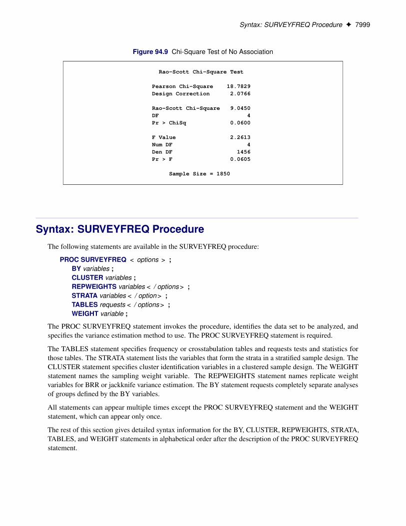
Figure 94.9 displays the chi-square test results. The Rao-Scott chi-square statistic equals 9.04, and thecorresponding F value is 2.26 with a p-value of 0.0605. This indicates an association between school type(middle school or high school) and satisfaction with the student information system at the 10% significancelevel.
Figure 94.8 Two-Way Table with Row Percentages
Student Information System Survey
The SURVEYFREQ Procedure
Table of SchoolType by Response
Std Err of Row Std Err ofSchoolType Response Frequency Percent Percent Percent Row Percent--------------------------------------------------------------------------------------------------Middle School Very Unsatisfied 116 6.4155 0.9030 15.8373 1.9920
Unsatisfied 109 6.1427 0.8283 15.1638 1.8140Neutral 234 12.4847 1.2953 30.8196 2.5173Satisfied 197 10.4467 1.1417 25.7886 2.2947Very Satisfied 94 5.0193 0.7758 12.3907 1.7449
Total 750 40.5089 2.5691 100.000--------------------------------------------------------------------------------------------------High School Very Unsatisfied 188 10.7521 1.1076 18.0735 1.6881
Unsatisfied 217 11.6137 1.1439 19.5218 1.7280Neutral 347 19.1119 1.4726 32.1255 2.0490Satisfied 258 13.4845 1.2823 22.6663 1.9240Very Satisfied 90 4.5290 0.6579 7.6128 1.0557
Total 1100 59.4911 2.5691 100.000--------------------------------------------------------------------------------------------------Total Very Unsatisfied 304 17.1676 1.2872
Unsatisfied 326 17.7564 1.2712Neutral 581 31.5965 1.5795Satisfied 455 23.9311 1.4761Very Satisfied 184 9.5483 0.9523
Total 1850 100.000--------------------------------------------------------------------------------------------------
Syntax: SURVEYFREQ Procedure F 7999
Figure 94.9 Chi-Square Test of No Association
Rao-Scott Chi-Square Test
Pearson Chi-Square 18.7829Design Correction 2.0766
Rao-Scott Chi-Square 9.0450DF 4Pr > ChiSq 0.0600
F Value 2.2613Num DF 4Den DF 1456Pr > F 0.0605
Sample Size = 1850
Syntax: SURVEYFREQ ProcedureThe following statements are available in the SURVEYFREQ procedure:
PROC SURVEYFREQ < options > ;BY variables ;CLUSTER variables ;REPWEIGHTS variables < / options > ;STRATA variables < / option > ;TABLES requests < / options > ;WEIGHT variable ;
The PROC SURVEYFREQ statement invokes the procedure, identifies the data set to be analyzed, andspecifies the variance estimation method to use. The PROC SURVEYFREQ statement is required.
The TABLES statement specifies frequency or crosstabulation tables and requests tests and statistics forthose tables. The STRATA statement lists the variables that form the strata in a stratified sample design. TheCLUSTER statement specifies cluster identification variables in a clustered sample design. The WEIGHTstatement names the sampling weight variable. The REPWEIGHTS statement names replicate weightvariables for BRR or jackknife variance estimation. The BY statement requests completely separate analysesof groups defined by the BY variables.
All statements can appear multiple times except the PROC SURVEYFREQ statement and the WEIGHTstatement, which can appear only once.
The rest of this section gives detailed syntax information for the BY, CLUSTER, REPWEIGHTS, STRATA,TABLES, and WEIGHT statements in alphabetical order after the description of the PROC SURVEYFREQstatement.

8000 F Chapter 94: The SURVEYFREQ Procedure
PROC SURVEYFREQ StatementPROC SURVEYFREQ < options > ;
The PROC SURVEYFREQ statement invokes the SURVEYFREQ procedure. It also identifies the data set tobe analyzed, specifies the variance estimation method to use, and provides sample design information. TheDATA= option names the input data set to be analyzed. The VARMETHOD= option specifies the varianceestimation method, which is the Taylor series method by default. For Taylor series variance estimation,you can include a finite population correction factor in the analysis by providing either the sampling rate orpopulation total with the RATE= or TOTAL= option. If your design is stratified with different sampling ratesor totals for different strata, you can input these stratum rates or totals in a SAS data set that contains thestratification variables.
Table 94.1 summarizes the options available in the PROC SURVEYFREQ statement.
Table 94.1 PROC SURVEYFREQ Statement Options
Option Description
DATA= Names the input SAS data setMISSING Treats missing values as a valid levelNOMCAR Treats missing values as not missing completely at randomNOSUMMARY Suppresses the display of the “Data Summary” tableORDER= Specifies the order of variable levelsPAGE Displays only one table per pageRATE= Specifies the first-stage sampling rateTOTAL= Specifies the total number of primary sampling unitsVARHEADER= Specifies the variable identification to displayVARMETHOD= Specifies the variance estimation method
You can specify the following options in the PROC SURVEYFREQ statement:
DATA=SAS-data-setnames the SAS-data-set to be analyzed by PROC SURVEYFREQ. If you omit the DATA= option, theprocedure uses the most recently created SAS data set.
MISSINGtreats missing values as a valid (nonmissing) category for all categorical variables, which includeTABLES, STRATA, and CLUSTER variables.
By default, if you do not specify the MISSING option, an observation is excluded from the analysis ifit has a missing value for any STRATA or CLUSTER variable. Additionally, PROC SURVEYFREQexcludes an observation from a frequency or crosstabulation table if that observation has a missingvalue for any of the variables in the table request, unless you specify the MISSING option. For moreinformation, see the section “Missing Values” on page 8033.

PROC SURVEYFREQ Statement F 8001
NOMCARincludes observations with missing values of TABLES variables in the variance computation as notmissing completely at random (NOMCAR) for Taylor series variance estimation. When you specify theNOMCAR option, PROC SURVEYFREQ computes variance estimates by analyzing the nonmissingvalues as a domain (subpopulation), where the entire population includes both nonmissing and missingdomains. For more information, see the section “Missing Values” on page 8033.
By default, PROC SURVEYFREQ completely excludes an observation from a frequency or crosstab-ulation table (and the corresponding variance computations) if that observation has a missing valuefor any of the variables in the table request, unless you specify the MISSING option. The NOMCARoption has no effect when you specify the MISSING option, which treats missing values as a validnonmissing level.
The NOMCAR option applies only to Taylor series variance estimation. The replication methods,which you request with the VARMETHOD=BRR and VARMETHOD=JACKKNIFE options, do notuse the NOMCAR option.
NOSUMMARYsuppresses the display of the “Data Summary” table, which PROC SURVEYFREQ produces by default.For information about this table, see the section “Data Summary Table” on page 8070.
ORDER=DATA | FORMATTED | FREQ | INTERNALspecifies the order of the variable levels in the frequency and crosstabulation tables, which you requestin the TABLES statement. The ORDER= option also controls the order of the STRATA variable levelsin the “Stratum Information” table.
The ORDER= option can take the following values:
ORDER= Levels Ordered By
DATA Order of appearance in the input data set
FORMATTED External formatted value, except for numeric variables withno explicit format, which are sorted by their unformatted(internal) value
FREQ Descending frequency count; levels with the most observa-tions come first in the order
INTERNAL Unformatted value
By default, ORDER=INTERNAL. The FORMATTED and INTERNAL orders are machine-dependent.The frequency count used by ORDER=FREQ is the nonweighted frequency (sample size), rather thanthe weighted frequency.
For more information about sort order, see the chapter on the SORT procedure in the Base SASProcedures Guide and the discussion of BY-group processing in SAS Language Reference: Concepts.
PAGEdisplays only one table per page. Otherwise, PROC SURVEYFREQ displays multiple tables per pageas space permits.

8002 F Chapter 94: The SURVEYFREQ Procedure
RATE=value
RATE=SAS-data-set
R=value
R=SAS-data-setspecifies the sampling rate, which PROC SURVEYFREQ uses to compute a finite population correctionfor Taylor series variance estimation. You can provide a single sampling rate value, or you can providestratum sampling rates by specifying a SAS-data-set .
If your sample design has multiple stages, you should specify the first-stage sampling rate, which isthe ratio of the number of primary sampling units (PSUs) in the sample to the total number of PSUs inthe population.
For a nonstratified sample design, or for a stratified sample design that uses the same sampling rate inall strata, you should specify a single sampling rate value. If your design is stratified and uses differentsampling rates in different strata, you should name a SAS-data-set that contains the stratificationvariables and the stratum sampling rates. You should provide the stratum sampling rates in the dataset variable named _RATE_. For more information, see the section “Population Totals and SamplingRates” on page 8032.
The sampling rate values must be nonnegative numbers. You can specify sampling rates as numbersbetween 0 and 1. Or you can specify sampling rates in percentage form as numbers between 1 and100, which PROC SURVEYFREQ converts to proportions. The procedure treats the value 1 as 100%instead of 1%.
If you do not specify the RATE= or the TOTAL= option, the Taylor series variance estimation does notinclude a finite population correction. You cannot specify both the RATE= and the TOTAL= option inthe same PROC SURVEYFREQ statement.
PROC SURVEYSELECT does not use the RATE= or the TOTAL= option for BRR or jack-knife variance estimation (which you can request by specifying the VARMETHOD=BRR orVARMETHOD=JACKKNIFE option, respectively).
TOTAL=value
TOTAL=SAS-data-set
N=value
N=SAS-data-setspecifies the total number of primary sampling units (PSUs), which PROC SURVEYFREQ uses tocompute a finite population correction for Taylor series variance estimation. You can provide a singletotal value, or you can provide stratum totals by specifying a SAS-data-set . The totals must be positivenumbers.
If your sample design has multiple stages, you should specify the total number of primary samplingunits (PSUs).
For a nonstratified sample design, you should specify a single total value, which refers to the totalnumber of PSUs in the population. For a stratified sample design that has the same population totalin each stratum, you can specify a single total value, which refers to the total number of PSUs ineach stratum. If your design is stratified and has different totals in different strata, you should namea SAS-data-set that contains the stratification variables and the stratum totals. You should providethe stratum totals in the data set variable named _TOTAL_. For more information, see the section“Population Totals and Sampling Rates” on page 8032.

PROC SURVEYFREQ Statement F 8003
If you do not specify the RATE= or the TOTAL= option, the Taylor series variance estimation does notinclude a finite population correction. You cannot specify both the RATE= and the TOTAL= option inthe same PROC SURVEYFREQ statement.
PROC SURVEYSELECT does not use the RATE= or the TOTAL= option for BRR or jack-knife variance estimation (which you can request by specifying the VARMETHOD=BRR orVARMETHOD=JACKKNIFE option, respectively).
VARHEADER=LABEL | NAME | NAMELABELspecifies the variable identification to use in the displayed output. By default VARHEADER=NAME,which displays variable names in the output. The VARHEADER= option affects the headers ofthe variable level columns in one-way frequency tables, crosstabulation tables, and the “StratumInformation” table. The VARHEADER= option also controls variable identification in the tableheaders.
The VARHEADER= option can take the following values:
VARHEADER= Variable Identification Displayed
LABEL Variable labelNAME Variable nameNAMELABEL Variable name and label, as Name (Label)
VARMETHOD=BRR < (method-options) >
VARMETHOD=JACKKNIFE | JK < (method-options) >
VARMETHOD=TAYLORspecifies the variance estimation method. VARMETHOD=TAYLOR requests the Taylor series method,which is the default if you do not specify the VARMETHOD= option or the REPWEIGHTS statement.VARMETHOD=BRR requests variance estimation by balanced repeated replication (BRR), andVARMETHOD=JACKKNIFE requests variance estimation by the delete-1 jackknife method.
For VARMETHOD=BRR and VARMETHOD=JACKKNIFE, you can specify method-options inparentheses after the variance method name. Table 94.2 summarizes the available method-options.
Table 94.2 Variance Estimation Options
VARMETHOD= Variance Estimation Method Method Options
BRR Balanced repeated replication DFADJFAY < =value >HADAMARD=SAS-data-setOUTWEIGHTS=SAS-data-setPRINTHREPS=number
JACKKNIFE | JK Jackknife DFADJOUTJKCOEFS=SAS-data-setOUTWEIGHTS=SAS-data-set
TAYLOR Taylor series linearization None

8004 F Chapter 94: The SURVEYFREQ Procedure
Method-options must be enclosed in parentheses after the variance method name. For example:
varmethod=BRR(reps=60 outweights=myReplicateWeights)
You can specify the following values for the VARMETHOD= option:
BRR < (method-options) >requests variance estimation by balanced repeated replication (BRR). The BRR method requiresa stratified sample design that has two primary sampling units (PSUs) in each stratum. If youspecify this option, you must also specify a STRATA statement unless you use a REPWEIGHTSstatement to provide replicate weights. For more information, see the section “Balanced RepeatedReplication (BRR)” on page 8043.
You can specify the following method-options:
DFADJcomputes the degrees of freedom as the number of nonmissing strata for the individual tablerequest. If you specify this option, PROC SURVEYFREQ does not count any empty stratathat occur when observations that have missing values of the TABLES variables are removedfrom the analysis of the table. By default, PROC SURVEYFREQ computes the degrees offreedom by counting the number of nonmissing strata for all valid observations in the inputdata set.
For more information, see the section “Degrees of Freedom” on page 8051. For informationabout valid observations, see the section “Data Summary Table” on page 8070.
This method-option has no effect when you specify the MISSING option, which treatsmissing values as a valid nonmissing level.
This method-option is not used when you specify the degrees of freedom in the DF= option inthe TABLES statement or when you specify a REPWEIGHTS statement to provide replicateweights. When you specify a REPWEIGHTS statement, the degrees of freedom are thenumber of REPWEIGHTS variables (replicates) unless you specify the DF= option in theREPWEIGHTS or the TABLES statement.
FAY < =value >requests Fay’s method, which is a modification of the BRR method. For more information,see the section “Fay’s BRR Method” on page 8044.
You can specify the value of the Fay coefficient, which is used in converting the originalsampling weights to replicate weights. The Fay coefficient must be a nonnegative numberless than 1. By default, the Fay coefficient is 0.5.
HADAMARD=SAS-data-setH=SAS-data-set
names a SAS-data-set that contains the Hadamard matrix for BRR replicate construction.If you do not specify this method-option, PROC SURVEYFREQ generates an appropriateHadamard matrix for replicate construction. For more information, see the sections “Bal-anced Repeated Replication (BRR)” on page 8043 and “Hadamard Matrix” on page 8045.
If a Hadamard matrix of a particular dimension exists, it is not necessarily unique. Therefore,if you want to use a specific Hadamard matrix, you must provide the matrix as a SAS-data-setin this method-option.

PROC SURVEYFREQ Statement F 8005
In the HADAMARD= input data set, each variable corresponds to a column and eachobservation corresponds to a row of the Hadamard matrix. You can use any variable namesin the HADAMARD= data set. All values in the data set must equal either 1 or –1. You mustensure that the matrix you provide is indeed a Hadamard matrix—that is, A0A D RI, whereA is the Hadamard matrix of dimension R and I is an identity matrix. PROC SURVEYFREQdoes not check the validity of the Hadamard matrix that you provide.
The HADAMARD= input data set must contain at least H variables, where H denotes thenumber of first-stage strata in your design. If the data set contains more than H variables,PROC SURVEYFREQ uses only the first H variables. Similarly, the HADAMARD= inputdata set must contain at least H observations.
If you do not specify the REPS= method-option, the number of replicates is assumed to be thenumber of observations in the HADAMARD= input data set. If you specify the number ofreplicates—for example, REPS=nreps—the first nreps observations in the HADAMARD=data set are used to construct the replicates.
You can specify the PRINTH method-option to display the Hadamard matrix that PROCSURVEYFREQ uses to construct replicates for BRR.
OUTWEIGHTS=SAS-data-setnames a SAS-data-set to store the replicate weights that PROC SURVEYFREQ createsfor BRR variance estimation. For information about replicate weights, see the section“Balanced Repeated Replication (BRR)” on page 8043. For information about the contentsof the OUTWEIGHTS= data set, see the section “Replicate Weight Output Data Set” onpage 8069.
The OUTWEIGHTS= method-option is not available when you provide replicate weights ina REPWEIGHTS statement.
PRINTHdisplays the Hadamard matrix that PROC SURVEYFREQ uses to construct replicates forBRR variance estimation. When you provide the Hadamard matrix in the HADAMARD=method-option, PROC SURVEYFREQ displays only the rows and columns that are actuallyused to construct replicates. For more information, see the sections “Balanced RepeatedReplication (BRR)” on page 8043 and “Hadamard Matrix” on page 8045.
The PRINTH method-option is not available when you provide replicate weights in aREPWEIGHTS statement because the procedure does not use a Hadamard matrix in thiscase.
REPS=numberspecifies the number of replicates for BRR variance estimation. The value of number mustbe an integer greater than 1.
If you do not use the HADAMARD= method-option to provide a Hadamard matrix, thenumber of replicates should be greater than the number of strata and should be a multipleof 4. For more information, see the section “Balanced Repeated Replication (BRR)” onpage 8043. If PROC SURVEYFREQ cannot construct a Hadamard matrix for the REPS=value that you specify, the value is increased until a Hadamard matrix of that dimension canbe constructed. Therefore, the actual number of replicates that PROC SURVEYFREQ usesmight be larger than number .

8006 F Chapter 94: The SURVEYFREQ Procedure
If you use the HADAMARD= method-option to provide a Hadamard matrix, the value ofnumber must not be less than the number of rows in the Hadamard matrix. If you provide aHadamard matrix and do not specify the REPS= method-option, the number of replicatesequals the number of rows in the Hadamard matrix.
If you do not specify the REPS= or the HADAMARD= method-option and do not use aREPWEIGHTS statement, the number of replicates equals the smallest multiple of 4 that isgreater than the number of strata.
If you use a REPWEIGHTS statement to provide replicate weights, PROC SURVEYFREQdoes not use the REPS= method-option; the number of replicates equals the number ofREPWEIGHTS variables.
JACKKNIFE < (method-options) >
JK < (method-options) >requests variance estimation by the delete-1 jackknife method. For more information, see thesection “The Jackknife Method” on page 8046. If you use a REPWEIGHTS statement to providereplicate weights, VARMETHOD=JACKKNIFE is the default variance estimation method.
The delete-1 jackknife method requires at least two primary sampling units (PSUs) in eachstratum for stratified designs unless you use a REPWEIGHTS statement to provide replicateweights.
You can specify the following method-options:
DFADJcomputes the degrees of freedom by using the number of nonmissing strata and clusters forthe individual table request. If you specify this method-option, PROC SURVEYFREQ doesnot count any empty strata or clusters that occur when observations that have missing valuesof the TABLES variables are removed from the analysis of the table. By default, PROCSURVEYFREQ computes the degrees of freedom by counting the number of nonmissingstrata and clusters for all valid observations in the input data set. The degrees of freedom forVARMETHOD=JACKKNIFE equal the number of clusters minus the number of strata.
For more information, see the section “Degrees of Freedom” on page 8051. For informationabout valid observations, see the section “Data Summary Table” on page 8070.
This method-option has no effect when you specify the MISSING option, which treatsmissing values as a valid nonmissing level.
This method-option is not used when you specify the degrees of freedom in the DF= option inthe TABLES statement or when you specify a REPWEIGHTS statement to provide replicateweights. When you specify a REPWEIGHTS statement, the degrees of freedom are thenumber of REPWEIGHTS variables (replicates) unless you specify the DF= option in theREPWEIGHTS or the TABLES statement.
OUTJKCOEFS=SAS-data-setnames a SAS-data-set to store the jackknife coefficients. For information about jackknifecoefficients, see the section “The Jackknife Method” on page 8046. For information aboutthe contents of the OUTJKCOEFS= data set, see the section “Jackknife Coefficient OutputData Set” on page 8070.

BY Statement F 8007
OUTWEIGHTS=SAS-data-setnames a SAS-data-set to store the replicate weights that PROC SURVEYFREQ creates forjackknife variance estimation. For information about replicate weights, see the section “TheJackknife Method” on page 8046. For information about the contents of the OUTWEIGHTS=data set, see the section “Replicate Weight Output Data Set” on page 8069.
This method-option is not available when you use a REPWEIGHTS statement to providereplicate weights.
TAYLORrequests Taylor series variance estimation. This is the default method if you do not specify theVARMETHOD= option or a REPWEIGHTS statement. For more information, see the section“Taylor Series Variance Estimation” on page 8036.
BY StatementBY variables ;
You can specify a BY statement with PROC SURVEYFREQ to obtain separate analyses of observations ingroups that are defined by the BY variables. When a BY statement appears, the procedure expects the inputdata set to be sorted in order of the BY variables. If you specify more than one BY statement, only the lastone specified is used.
If your input data set is not sorted in ascending order, use one of the following alternatives:
• Sort the data by using the SORT procedure with a similar BY statement.
• Specify the NOTSORTED or DESCENDING option in the BY statement for the SURVEYFREQprocedure. The NOTSORTED option does not mean that the data are unsorted but rather that thedata are arranged in groups (according to values of the BY variables) and that these groups are notnecessarily in alphabetical or increasing numeric order.
• Create an index on the BY variables by using the DATASETS procedure (in Base SAS software).
Using a BY statement provides completely separate analyses of the BY groups. It does not provide astatistically valid domain (subpopulation) analysis, where the total number of units in the subpopulation isnot known with certainty. You should include the domain variable(s) in your TABLES request to obtaindomain analysis. For more information, see the section “Domain Analysis” on page 8033.
For more information about BY-group processing, see the discussion in SAS Language Reference: Concepts.For more information about the DATASETS procedure, see the discussion in the Base SAS Procedures Guide.

8008 F Chapter 94: The SURVEYFREQ Procedure
CLUSTER StatementCLUSTER variables ;
The CLUSTER statement names variables that identify the first-stage clusters in a clustered sample design.First-stage clusters are also known as primary sampling units (PSUs). The combinations of categories ofCLUSTER variables define the clusters in the sample. If there is a STRATA statement, clusters are nestedwithin strata.
If your sample design has clustering at multiple stages, you should specify only the first-stage clusters(PSUs) in the CLUSTER statement. See the section “Specifying the Sample Design” on page 8031 for moreinformation.
If you provide replicate weights for BRR or jackknife variance estimation with the REPWEIGHTS statement,you do not need to specify a CLUSTER statement.
The CLUSTER variables are one or more variables in the DATA= input data set. These variables can beeither character or numeric, but the procedure treats them as categorical variables. The formatted valuesof the CLUSTER variables determine the CLUSTER variable levels. Thus, you can use formats to groupvalues into levels. See the discussion of the FORMAT procedure in the Base SAS Procedures Guide and thediscussions of the FORMAT statement and SAS formats in SAS Formats and Informats: Reference.
An observation is excluded from the analysis if it has a missing value for any CLUSTER variable unless youspecify the MISSING option in the PROC SURVEYFREQ statement. See the section “Missing Values” onpage 8033 for more information.
You can use multiple CLUSTER statements to specify CLUSTER variables. The procedure uses variablesfrom all CLUSTER statements to create clusters.
REPWEIGHTS StatementREPWEIGHTS variables < / options > ;
The REPWEIGHTS statement names variables that provide replicate weights for BRR or jackknife varianceestimation, which you can request by specifying the VARMETHOD=BRR or VARMETHOD=JACKKNIFEoption in the PROC SURVEYFREQ statement. If you do not provide replicate weights for these methods byusing a REPWEIGHTS statement, then PROC SURVEYFREQ constructs replicate weights for the analysis.See the sections “Balanced Repeated Replication (BRR)” on page 8043 and “The Jackknife Method” onpage 8046 for information about replicate weights.
Each REPWEIGHTS variable should contain the weights for a single replicate, and the number of replicatesequals the number of REPWEIGHTS variables. The REPWEIGHTS variables must be numeric, and thevariable values must be nonnegative numbers.
If you provide replicate weights with a REPWEIGHTS statement, you do not need to specify a CLUSTER orSTRATA statement. If you use a REPWEIGHTS statement and do not specify the VARMETHOD= option inthe PROC SURVEYFREQ statement, the procedure uses VARMETHOD=JACKKNIFE by default.

REPWEIGHTS Statement F 8009
If you specify a REPWEIGHTS statement but do not include a WEIGHT statement, PROC SURVEYFREQuses the average of each observation’s replicate weights as the observation’s weight.
You can specify the following options in the REPWEIGHTS statement after a slash (/):
DF=dfspecifies the degrees of freedom for the analysis. The value of df must be a positive number. Bydefault, the degrees of freedom equal the number of REPWEIGHTS variables. For more information,see the section “Degrees of Freedom” on page 8051.
PROC SURVEYFREQ uses the value df to obtain the t-percentile for confidence limits for proportions,totals, and other statistics. For more information, see the section “Confidence Limits for Proportions”on page 8048. PROC SURVEYFREQ also uses df to compute the denominator degrees of freedom forthe F statistics in the Rao-Scott and Wald chi-square tests. For more information, see the sections “Rao-Scott Chi-Square Test” on page 8060, “Rao-Scott Likelihood Ratio Chi-Square Test” on page 8065,“Wald Chi-Square Test” on page 8067, and “Wald Log-Linear Chi-Square Test” on page 8068.
JKCOEFS=value
JKCOEFS=(values)
JKCOEFS=SAS-data-setspecifies the jackknife coefficients for jackknife variance estimation (which you can request byspecifying VARMETHOD=JACKKNIFE). You can provide a single jackknife coefficient value touse for all replicates, or you can provide a value for each replicate by specifying a list of values or aSAS-data-set . The jackknife coefficient values must be nonnegative numbers. For more information,see the section “The Jackknife Method” on page 8046.
You can provide jackknife coefficients by specifying one of the following forms:
valuespecifies a single jackknife coefficient value to use for all replicates. The coefficient value mustbe a nonnegative number.
(values)specifies a list of jackknife coefficient values, where each value corresponds to a single replicatethat is identified by a REPWEIGHTS variable. You can separate the values with blanks orcommas. The coefficient values must be nonnegative numbers. The number of coefficient valuesshould equal the number of replicate weight variables that you specify in the REPWEIGHTSstatement.
You should list the jackknife coefficient values in the same order in which you list the correspond-ing replicate weight variables in the REPWEIGHTS statement.
SAS-data-setnames a SAS-data-set that contains the jackknife coefficients. You should provide the jackknifecoefficients in the data set variable named JKCoefficient. Each coefficient value must be anonnegative number. Each observation in this data set should correspond to a replicate that isidentified by a REPWEIGHTS variable. The number of observations in this data set must not beless than the number of REPWEIGHTS variables.

8010 F Chapter 94: The SURVEYFREQ Procedure
STRATA StatementSTRATA variables < / option > ;
The STRATA statement names variables that identify the first-stage strata in a stratified sample design. Thecombinations of levels of STRATA variables define the strata in the sample, where strata are nonoverlappingsubgroups that were sampled independently.
If your sample design has stratification at multiple stages, you should specify only the first-stage strata in theSTRATA statement. See the section “Specifying the Sample Design” on page 8031 for more information.
If you use a REPWEIGHTS statement to provide replicate weights for BRR or jackknife variance estimation,you do not need to specify a STRATA statement.
The STRATA variables are one or more variables in the DATA= input data set. These variables can be eithercharacter or numeric, but the procedure treats them as categorical variables. The formatted values of theSTRATA variables determine the STRATA variable levels. Thus, you can use formats to group values intolevels. See the discussion of the FORMAT procedure in the Base SAS Procedures Guide and the discussionsof the FORMAT statement and SAS formats in SAS Formats and Informats: Reference.
PROC SURVEYFREQ excludes an observation from the analysis if it has a missing value for any STRATAvariable unless you specify the MISSING option in the PROC SURVEYFREQ statement. For more informa-tion, see the section “Missing Values” on page 8033.
You can use multiple STRATA statements to specify STRATA variables. The procedure uses variables fromall STRATA statements to define strata.
You can specify the following option in the STRATA statement after a slash (/):
LISTdisplays the “Stratum Information” table, which lists all strata together with the corresponding valuesof the STRATA variables. This table provides the number of observations and the number of clustersin each stratum, as well as the sampling fraction if you specify the RATE= or TOTAL= option in thePROC SURVEYFREQ statement. See the section “Stratum Information Table” on page 8071 for moreinformation.
TABLES StatementTABLES requests < / options > ;
The TABLES statement requests one-way to n-way frequency and crosstabulation tables and statistics forthese tables.
If you omit the TABLES statement, PROC SURVEYFREQ generates one-way frequency tables for allDATA= data set variables that are not listed in the other statements.
The following argument is required in the TABLES statement:
requestsspecify the frequency and crosstabulation tables to produce. A request is composed of one variablename or several variable names separated by asterisks. To request a one-way frequency table, use asingle variable. To request a two-way crosstabulation table, use an asterisk between two variables. Torequest a multiway table (an n-way table, where n > 2), separate the desired variables with asterisks.The unique values of these variables form the rows, columns, and layers of the table.

TABLES Statement F 8011
For two-way tables to multiway tables, the values of the last variable form the crosstabulation tablecolumns, while the values of the next-to-last variable form the rows. Each level (or combination oflevels) of the other variables forms one layer. PROC SURVEYFREQ produces a separate crosstabula-tion table for each layer. For example, a specification of A*B*C*D in a TABLES statement produces ktables, where k is the number of different combinations of levels for A and B. Each table lists the levelsfor D (columns) within each level of C (rows).
You can use multiple TABLES statements in a single PROC SURVEYFREQ step. You can also specifyany number of table requests in a single TABLES statement. To specify multiple table requests quickly,use a grouping syntax by placing parentheses around several variables and joining other variables orvariable combinations. Table 94.3 shows some examples of grouping syntax.
Table 94.3 Grouping Syntax
TABLES Request Equivalent to
A*(B C) A*B A*C(A B)*(C D) A*C B*C A*D B*D(A B C)*D A*D B*D C*DA – – C A B C(A – – C)*D A*D B*D C*D
The TABLES statement variables are one or more variables from the DATA= input data set. These vari-ables can be either character or numeric, but the procedure treats them as categorical variables. PROCSURVEYFREQ uses the formatted values of the TABLES variable to determine the categorical variablelevels. So if you assign a format to a variable with a FORMAT statement, PROC SURVEYFREQformats the values before dividing observations into the levels of a frequency or crosstabulation table.See the discussion of the FORMAT procedure in the Base SAS Procedures Guide and the discussionsof the FORMAT statement and SAS formats in SAS Formats and Informats: Reference.
By default, the frequency or crosstabulation table lists the values of both character and numericvariables in ascending order based on internal (unformatted) variable values. You can change the orderof the values in the table by specifying the ORDER= option in the PROC SURVEYFREQ statement.To list the values in ascending order by formatted value, use ORDER=FORMATTED.
Without Options
If you request a frequency or crosstabulation table without specifying options, PROC SURVEYFREQproduces the following for each table level or cell:
• frequency (sample size)
• weighted frequency, which estimates the population total
• standard deviation of the weighted frequency
• percentage, which estimates the population proportion
• standard error of the percentage
The table displays weighted frequencies if your analysis includes a WEIGHT statement, or if you specifythe WTFREQ option in the TABLES statement. The table also displays the number of observations withmissing values. See the sections “One-Way Frequency Tables” on page 8072 and “Crosstabulation Tables”on page 8073 for more information.

8012 F Chapter 94: The SURVEYFREQ Procedure
Options
Table 94.4 summarizes the options available in the TABLES statement. Descriptions of the options followthe table in alphabetical order.
Table 94.4 TABLES Statement Options
Option Description
Control Statistical AnalysisAGREE Requests kappa coefficientsALPHA= Sets level for confidence limitsCHISQ Requests Rao-Scott chi-square testDF= Specifies degrees of freedomKAPPA Requests simple kappa coefficientLRCHISQ Requests Rao-Scott likelihood ratio testOR Requests odds ratio and relative risksRISK Requests risks and risk differenceTESTP= Specifies null proportions for one-way chi-square testWCHISQ Requests Wald chi-square testWLLCHISQ Requests Wald log-linear chi-square testWTKAPPA Requests weighted kappa coefficient
Request Additional Table InformationCELLCHI2 Displays cell contributions to the Pearson chi-squareCL Displays confidence limits for percentages and
specifies confidence limit type for percentagesCLWT Displays confidence limits for weighted frequenciesCOLUMN Displays column percentages and standard errorsCV Displays coefficients of variation for percentagesCVWT Displays coefficients of variation for weighted frequenciesDEFF Displays design effects for percentagesDEVIATION Displays deviations of weighted frequenciesEXPECTED Displays expected weighted frequenciesPEARSONRES Displays Pearson residualsROW Displays row percentages and standard errorsVAR Displays variances of percentagesVARWT Displays variances of weighted frequenciesWTFREQ Displays totals and standard errors
when there is no WEIGHT statement
Control Displayed OutputNOCELLPERCENT Suppresses display of overall percentagesNOFREQ Suppresses display of frequency countsNOPERCENT Suppresses display of all percentagesNOPRINT Suppresses display of tables but displays statistical testsNOSPARSE Suppresses display of zero rows and columnsNOSTD Suppresses display of standard errors for all estimatesNOTOTAL Suppresses display of row and column totalsNOWT Suppresses display of weighted frequencies
Produce Statistical GraphicsPLOTS= Requests plots from ODS Graphics

TABLES Statement F 8013
You can specify the following options in a TABLES statement:
AGREE < (options) >requests the simple and weighted kappa coefficients with their standard errors and confidence limits.Kappa coefficients can be computed for square two-way tables, where the number of rows equals thenumber of columns. For 2�2 tables, the weighted kappa coefficient equals the simple kappa coefficient,and PROC SURVEYFREQ displays only the simple kappa coefficient. For more information, see thesection “Kappa Coefficients” on page 8057.
Kappa coefficients are available when you specify variance estimation by the jackknife method(VARMETHOD=JACKKNIFE) or by balanced repeated replication (VARMETHOD=BRR); kappacoefficients are not available with the Taylor series method (VARMETHOD=TAYLOR).
The weighted kappa coefficient is computed by using agreement weights that reflect the relativeagreement between pairs of variable levels. Agreement weights are not the same as sampling weights,which you provide by specifying the WEIGHT statement. PROC SURVEYFREQ uses samplingweights to compute both the simple and weighted kappa coefficients. For more information, see thesection “Weighted Kappa Coefficient” on page 8058.
To compute confidence limits for the kappa coefficient, PROC SURVEYFREQ determines the confi-dence coefficient from the ALPHA= option, which by default equals 0.05 and produces 95% confidencelimits.
You can request the simple kappa coefficient or the weighted kappa coefficient separately by specifyingthe KAPPA or WTKAPPA option, respectively.
You can specify the following options:
PRINTKWTSdisplays the agreement weights that PROC SURVEYFREQ uses to compute the weighted kappacoefficient. Agreement weights reflect the relative agreement between pairs of variable levels. Bydefault, PROC SURVEYFREQ uses the Cicchetti-Allison form of agreement weights. If youspecify the WT=FC option, the procedure uses the Fleiss-Cohen form of agreement weights. Formore information, see the section “Weighted Kappa Coefficient” on page 8058.
WT=FCrequests Fleiss-Cohen agreement weights for the weighted kappa computation. By default,PROC SURVEYFREQ uses Cicchetti-Allison agreement weights to compute the weighted kappacoefficient. Agreement weights reflect the relative agreement between pairs of variable levels.For more information, see the section “Weighted Kappa Coefficient” on page 8058.
ALPHA=˛sets the level for confidence limits. The value of ˛ must be between 0 and 1, and the default is 0.05. Aconfidence level of ˛ produces 100.1 � ˛/% confidence limits. The default of ALPHA=0.05 produces95% confidence limits.
You request confidence limits for percentages with the CL option, and you request confidence limitsfor weighted frequencies with the CLWT option. See the sections “Confidence Limits for Proportions”on page 8048 and “Confidence Limits for Totals” on page 8048 for more information.
The ALPHA= option also applies to confidence limits for the risks and risk difference, which yourequest with the RISK option, and to confidence limits for the odds ratio and relative risks, which yourequest with the OR option. See the sections “Risks and Risk Difference” on page 8054 and “OddsRatio and Relative Risks” on page 8055 for details.

8014 F Chapter 94: The SURVEYFREQ Procedure
CELLCHI2displays each table cell’s contribution to the Pearson chi-square statistic in the crosstabulation table.The cell chi-square is computed as .weighted frequency � expected/2 = expected, where weightedfrequency is the weighted frequency of the table cell and expected is the expected weighted frequency,which is computed under the null hypothesis that the row and column variables are independent. Youcan display the expected weighted frequencies by specifying the EXPECTED option, and you candisplay the deviations (weighted frequency – expected) by specifying the DEVIATION option. Formore information, see the sections “Expected Weighted Frequency” on page 8053 and “Rao-ScottChi-Square Test” on page 8060. This option has no effect for one-way tables.
CHISQ < (options) >requests the Rao-Scott chi-square test. This is a design-adjusted test that is computed by applyinga design correction to the weighted Pearson chi-square statistic. By default, PROC SURVEYFREQprovides a first-order Rao-Scott chi-square test. If you specify CHISQ(SECONDORDER), the proce-dure provides a second-order (Satterthwaite) Rao-Scott chi-square test. See the section “Rao-ScottChi-Square Test” on page 8060 for details.
For one-way tables, the CHISQ option produces a design-based goodness-of-fit test. By default,this is a goodness-of-fit test for equal proportions. If you specify the null hypothesis proportions inthe TESTP= option, the CHISQ option produces a chi-square goodness-of-fit test for the specifiedproportions.
By default for one-way tables, and for first-order tests for two-way tables, the design correction iscomputed from proportion estimates. If you specify CHISQ(MODIFIED), the design correction iscomputed from null hypothesis proportions. For second-order tests for two-way tables, the designcorrection is always computed from null hypothesis proportions.
You can specify the following options:
FIRSTORDERrequests a first-order Rao-Scott chi-square test. This is the default for the CHISQ option; if youdo not specify CHISQ(SECONDORDER), the procedure provides a first-order Rao-Scott test.
MODIFIEDuses the null hypothesis proportions to compute the Rao-Scott design correction. By default (ifyou do not specify CHISQ(MODIFIED)), the procedure uses proportion estimates to computethe design correction for all first-order tests and for second-order tests for one-way tables. Forsecond-order tests for two-way tables, the procedure always uses null hypothesis proportions tocompute the design correction.
SECONDORDERrequests a second-order (Satterthwaite) Rao-Scott chi-square test. See the section “Rao-ScottChi-Square Test” on page 8060 for details.
CL < (options) >requests confidence limits for the percentages (proportions) in the crosstabulation table. By default,PROC SURVEYFREQ computes standard Wald (“linear”) confidence limits for proportions by usingthe variance estimates that are based on the sample design. See the section “Confidence Limits forProportions” on page 8048 for more information. The procedure determines the confidence coefficientfrom the ALPHA= option, which by default equals 0.05 and produces 95% confidence limits.

TABLES Statement F 8015
You can specify options in parentheses after the CL option to control the confidence limit computations.You can use the TYPE= option to request an alternative confidence limit type. In addition to Waldconfidence limits, the following types of design-based confidence limits are available for proportions:modified Clopper-Pearson (exact), modified Wilson (score), and logit confidence limits.
If you specify the PSMALL option, PROC SURVEYFREQ uses the alternative confidence limittype for extreme (small or large) proportion estimates and uses Wald confidence limits for all otherproportion estimates. If you do not specify the PSMALL option, PROC SURVEYFREQ computes thespecified confidence limit type for all proportion values.
You can specify the following options:
ADJUST=NO | YEScontrols the degrees-of-freedom adjustment to the effective sample size for the modified Clopper-Pearson and Wilson confidence limits. By default, ADJUST=YES. If you specify ADJUST=NO,the confidence limit computations do not apply the degrees-of-freedom adjustment to the effectivesample size. See the section “Modified Confidence Limits” on page 8049 for details.
The ADJUST= option is available for TYPE=CLOPPERPEARSON and TYPE=WILSON confi-dence limits.
PSMALL < =p >uses the alternative confidence limit type that you specify with the TYPE= option for extreme(small or large) proportion values.
The PSMALL value p defines the range of extreme proportion values, where those proportionsless than or equal to p or greater than or equal to (1 – p) are considered to be extreme, and thoseproportions between p and (1 – p) are not extreme. If you do not specify a PSMALL value p,PROC SURVEYFREQ uses p = 0.25 by default. For p D 0:25, the procedure computes Waldconfidence limits for proportions between 0.25 and 0.75 and computes the alternative confidencelimit type for proportions less than or equal to 0.25 or greater than or equal to 0.75.
The PSMALL value p must be a nonnegative number. You can specify p as a proportion between0 and 0.5. Or you can specify p in percentage form as a number between 1 and 50, and PROCSURVEYFREQ converts that number to a proportion. The procedure treats the value 1 as thepercentage form 1%.
The PSMALL option is available for TYPE=CLOPPERPEARSON, TYPE=LOGIT, andTYPE=WILSON confidence limits. See the section “Confidence Limits for Proportions” onpage 8048 for details.
TRUNCATE=NO | YEScontrols the truncation of the effective sample size for the modified Clopper-Pearson and Wilsonconfidence limits. By default, TRUNCATE=YES truncates the effective sample size if it is largerthan the original sample size. If you specify TRUNCATE=NO, the effective sample size is nottruncated. See the section “Modified Confidence Limits” on page 8049 for details.
The TRUNCATE= option is available for TYPE=CLOPPERPEARSON and TYPE=WILSONconfidence limits.

8016 F Chapter 94: The SURVEYFREQ Procedure
TYPE=typespecifies the type of confidence limits to compute for proportions. If you do not specify theTYPE= option, PROC SURVEYFREQ computes Wald confidence limits (TYPE=WALD) bydefault.
If you specify the CL(PSMALL) option, the procedure uses the specified confidence limit type forextreme proportions (outside the PSMALL range) and uses Wald confidence limits for proportionsthat are not outside the range. If you do not specify the CL(PSMALL) option, the procedure usesthe specified confidence limit type for all proportions.
You can specify one of the following confidence limit types:
CLOPPERPEARSON
CPrequests modified Clopper-Pearson (exact) confidence limits for proportions. See the section“Modified Clopper-Pearson Confidence Limits” on page 8050 for details.
LOGITrequests logit confidence limits for proportions. See the section “Logit Confidence Limits”on page 8050 for details.
WALDrequests standard Wald (“linear”) confidence limits for proportions. This is the defaultconfidence limit type if you do not specify the TYPE= option. See the section “WaldConfidence Limits” on page 8049 for details.
WILSON
SCORErequests modified Wilson (score) confidence limits for proportions. See the section “ModifiedWilson Confidence Limits” on page 8050 for details.
CLWTrequests confidence limits for the weighted frequencies (totals) in the crosstabulation table. PROCSURVEYFREQ determines the confidence coefficient from the ALPHA= option, which by defaultequals 0.05 and produces 95% confidence limits. See the section “Confidence Limits for Totals” onpage 8048 for more information.
COLUMN < (option) >displays the column percentage (estimated proportion of the column total) for each cell in a two-waytable. The COLUMN option also provides the standard errors of the column percentages. See thesection “Row and Column Proportions” on page 8042 for more information. This option has no effectfor one-way tables.
You can specify the following option:
DEFFdisplays the design effect for each column percentage in the crosstabulation table. See the section“Design Effect” on page 8052 for more information.

TABLES Statement F 8017
CVdisplays the coefficient of variation for each percentage (proportion) estimate in the crosstabulationtable. See the section “Coefficient of Variation” on page 8052 for more information.
CVWTdisplays the coefficient of variation for each weighted frequency (estimated total), in the crosstabulationtable. See the section “Coefficient of Variation” on page 8052 for more information.
DEFFdisplays the design effect for each overall percentage (proportion) estimate in the crosstabulation table.See the section “Design Effect” on page 8052 for more information.
To request design effects for row or column percentages, specify the DEFF option in parentheses afterthe ROW or COLUMN option.
DEVIATIONdisplays the deviations of the weighted frequencies from the expected weighted frequencies (weightedfrequency – expected) in the crosstabulation table. The expected weighted frequencies are computedunder the null hypothesis that the row and column variables are independent. You can display theexpected values by specifying the EXPECTED option. For more information, see the section “ExpectedWeighted Frequency” on page 8053. This option has no effect for one-way tables.
DF=dfspecifies the degrees of freedom for the analysis. The value of df must be a nonnegative number. Bydefault, PROC SURVEYFREQ computes the degrees of freedom as described in the section “Degreesof Freedom” on page 8051.
PROC SURVEYFREQ uses the value df to obtain the t-percentile for confidence limits for proportions,totals, and other statistics. For more information, see the section “Confidence Limits for Proportions”on page 8048. PROC SURVEYFREQ also uses df to compute the denominator degrees of freedom forthe F statistics in the Rao-Scott and Wald chi-square tests. For more information, see the sections “Rao-Scott Chi-Square Test” on page 8060, “Rao-Scott Likelihood Ratio Chi-Square Test” on page 8065,“Wald Chi-Square Test” on page 8067, and “Wald Log-Linear Chi-Square Test” on page 8068.
EXPECTEDdisplays the expected weighted frequencies for the cells in the crosstabulation table. The expectedweighted frequencies are computed under the null hypothesis that the row and column variables areindependent. See the section “Expected Weighted Frequency” on page 8053 for more information.This option has no effect for one-way tables.
KAPPArequests the simple kappa coefficient with its standard error and confidence limits. The kappa coefficientcan be computed for square two-way tables, where the number of rows equals the number of columns.For more information, see the section “Simple Kappa Coefficient” on page 8057.
The kappa coefficient is available when you specify variance estimation by the jackknife method(VARMETHOD=JACKKNIFE) or by balanced repeated replication (VARMETHOD=BRR); the kappacoefficient is not available with the Taylor series method (VARMETHOD=TAYLOR).
To compute confidence limits for the kappa coefficient, PROC SURVEYFREQ determines the confi-dence coefficient from the ALPHA= option, which by default equals 0.05 and produces 95% confidencelimits.

8018 F Chapter 94: The SURVEYFREQ Procedure
LRCHISQ < (options) >requests the Rao-Scott likelihood ratio chi-square test. This is a design-adjusted test that is com-puted by applying a design correction to the weighted likelihood ratio chi-square statistic. By de-fault, PROC SURVEYFREQ provides a first-order Rao-Scott likelihood ratio test. If you specifyLRCHISQ(SECONDORDER), the procedure provides a second-order (Satterthwaite) Rao-Scott like-lihood ratio test. See the section “Rao-Scott Likelihood Ratio Chi-Square Test” on page 8065 fordetails.
For one-way tables, the LRCHISQ option produces a design-based likelihood ratio goodness-of-fit test.By default, the null hypothesis is equal proportions. If you specify null hypothesis proportions in theTESTP= option, the LRCHISQ option produces a design-based likelihood ratio test for the specifiedproportions.
By default for one-way tables, and for first-order tests for two-way tables, the design correction iscomputed from proportion estimates. If you specify LRCHISQ(MODIFIED), the design correctionis computed from null hypothesis proportions. For second-order tests for two-way tables, the designcorrection is always computed from null hypothesis proportions.
You can specify the following options:
FIRSTORDERrequests a first-order Rao-Scott likelihood ratio test. This is the default for the LRCHISQoption; if you do not specify LRCHISQ(SECONDORDER), the procedure provides a first-orderRao-Scott test.
MODIFIEDuses the null hypothesis proportions to compute the Rao-Scott design correction. By default (ifyou do not specify LRCHISQ(MODIFIED)), the procedure uses proportion estimates to computethe design correction for all first-order tests and for second-order tests for one-way tables. Forsecond-order tests for two-way tables, the procedure always uses null hypothesis proportions tocompute the design correction.
SECONDORDERrequests a second-order (Satterthwaite) Rao-Scott likelihood ratio test. See the section “Rao-ScottLikelihood Ratio Chi-Square Test” on page 8065 for details.
NOCELLPERCENTsuppresses the display of overall cell percentages in the crosstabulation table, as well as the standarderrors of the percentages. The NOCELLPERCENT option does not suppress the display of row orcolumn percentages, which you request with the ROW or COLUMN option.
NOFREQsuppresses the display of cell frequencies in the crosstabulation table. The NOFREQ option alsosuppresses the display of row, column, and overall table frequencies.
NOPERCENTsuppresses the display of all percentages in the crosstabulation table. The NOPERCENT option alsosuppresses the display of standard errors of the percentages. Use the NOCELLPERCENT option tosuppress display of overall cell percentages but allow display of row or column percentages.

TABLES Statement F 8019
NOPRINTsuppresses the display of frequency and crosstabulation tables but displays all requested statisticaltests. This option disables the Output Delivery System (ODS) for the suppressed tables. For moreinformation, see Chapter 20, “Using the Output Delivery System.”
NOSPARSEsuppresses the display of variable levels with zero frequency in two-way tables. By default, theprocedure displays all levels of the column variable within each level of the row variable, including anycolumn variable levels with zero frequency for that row. For multiway tables, the procedure displaysall levels of the row variable for each layer of the table by default, including any row variable levelswith zero frequency for the layer.
NOSTDsuppresses the display of all standard errors in the crosstabulation table.
NOTOTALsuppresses the display of row totals, column totals, and overall totals in the crosstabulation table.
NOWTsuppresses the display of weighted frequencies in the crosstabulation table. The NOWT option alsosuppresses the display of standard errors of the weighted frequencies.
OR
RELRISKrequests estimates of the odds ratio, the column 1 relative risk, and the column 2 relative risk for 2 � 2tables. The OR option also provides confidence limits for these statistics. See the section “Odds Ratioand Relative Risks” on page 8055 for details.
To compute confidence limits for the odds ratio and relative risks, PROC SURVEYFREQ determinesthe confidence coefficient from the ALPHA= option, which by default equals 0.05 and produces 95%confidence limits.
PEARSONRESdisplays each crosstabulation table cell’s Pearson residual, which is the square root of the ta-ble cell’s contribution to the Pearson chi-square statistic. The Pearson residual is computed as.weighted frequency � expected/ =
pexpected, where weighted frequency is the weighted frequency
of the table cell and expected is the expected weighted frequency, which is computed under the nullhypothesis that the row and column variables are independent. You can display the expected values,the deviations, and the cell chi-squares by specifying the EXPECTED, DEVIATION, and CELLCHI2options, respectively. For more information, see the sections “Expected Weighted Frequency” onpage 8053 and “Rao-Scott Chi-Square Test” on page 8060. This option has no effect for one-waytables.

8020 F Chapter 94: The SURVEYFREQ Procedure
PLOTS < (global-plot-options) > < =plot-request < (plot-options) > >
PLOTS < (global-plot-options) >
< =(plot-request < (plot-options) > < . . . plot-request < (plot-options) > > ) >controls the plots that are produced through ODS Graphics. Plot-requests identify the plots, andplot-options control the appearance and content of the plots. You can specify plot-options in parenthesesafter a plot-request . A global-plot-option applies to all plots for which it is available unless it is alteredby a specific plot-option. You can specify global-plot-options in parentheses after the PLOTS option.
When you specify only one plot-request , you can omit the parentheses around the plot-request . Forexample:
plots=allplots=wtfreqplotplots=(wtfreqplot oddsratioplot)plots(only)=(riskdiffplot relriskplot)
ODS Graphics must be enabled before plots can be requested. For example:
ods graphics on;proc surveyfreq;
tables treatment*response / chisq plots=wtfreqplot;weight wt;
run;ods graphics off;
For more information about enabling and disabling ODS Graphics, see the section “Enabling andDisabling ODS Graphics” on page 606 in Chapter 21, “Statistical Graphics Using ODS.”
If ODS Graphics is enabled but you do not specify the PLOTS= option, PROC SURVEYFREQproduces all plots that are associated with the analyses that you request, with the exception of weightedfrequency plots and mosaic plots. To produce a weighted frequency plot or mosaic plot when ODSGraphics is enabled, you must specify the WTFREQPLOT or MOSAICPLOT plot-request, or youmust specify the PLOTS=ALL option. PROC SURVEYFREQ produces the remaining plots (listed inTable 94.5) by default when you request the corresponding TABLES statement options.
You can suppress default plots and request specific plots by using the PLOTS(ONLY)= option;PLOTS(ONLY)=(plot-requests) produces only the plots that are specified as plot-requests. You cansuppress all plots by specifying the PLOTS=NONE option.
See Figure 94.4 and Figure 94.7 for examples of plots that PROC SURVEYFREQ produces. Forgeneral information about ODS Graphics, see Chapter 21, “Statistical Graphics Using ODS.”

TABLES Statement F 8021
Plot Requests
Table 94.5 lists the available plot-requests together with their required TABLES statement options.Descriptions of the plot-requests follow the table in alphabetical order.
Table 94.5 Plot Requests
Plot Request Description Required TABLES Statement Option
ALL All plots NoneKAPPAPLOT Kappa plot AGREE or KAPPA (h � r � r table)MOSAICPLOT Mosaic plot Crosstabulation table requestNONE No plots NoneODDSRATIOPLOT Odds ratio plot OR (h � 2 � 2 table)RELRISKPLOT Relative risk plot OR (h � 2 � 2 table)RISKDIFFPLOT Risk difference plot RISK, RISK1, or RISK2 (h � 2 � 2 table)WTFREQPLOT Weighted frequency plot Frequency or crosstabulation table requestWTKAPPAPLOT Weighted kappa plot AGREE or WTKAPPA (h � r � r table, r > 2)
The following plot-requests are available with the PLOTS= option:
ALLrequests all plots that are associated with the specified analyses. If you specify the PLOTS=ALLoption, PROC SURVEYFREQ also produces the weighted frequency and mosaic plots that areassociated with the tables that you request. (PROC SURVEYFREQ does not produce weightedfrequency and mosaic plots by default when ODS Graphics is enabled.)
KAPPAPLOT < (plot-options) >requests a plot of kappa coefficients with confidence limits. Kappa plots are available for multiwaysquare tables and display the simple kappa coefficient (with confidence limits) for each two-waytable layer. To produce a kappa plot, you must specify the KAPPA or AGREE option in theTABLES statement to compute kappa coefficients.
Table 94.6 lists the plot-options that are available for kappa plots. For descriptions of theplot-options, see the subsection “Plot Options.”
Table 94.6 Plot Options for KAPPAPLOT and WTKAPPAPLOT
Plot Option Description Values
CLDISPLAY= Error bar type SERIF�, SERIFARROW,LINE, LINEARROW, or BAR
NPANELPOS= Statistics per graphic Number (All�)ORDER= Order of two-way levels ASCENDING or DESCENDINGRANGE= Range to display Values or CLIPSTATS Statistic values None�Default

8022 F Chapter 94: The SURVEYFREQ Procedure
MOSAICPLOT < (plot-options) >requests a mosaic plot. Mosaic plots are available for crosstabulation tables. For multiway tables,PROC SURVEYFREQ provides a mosaic plot for each two-way table layer.
To produce a mosaic plot, you must specify the MOSAICPLOT plot-request in the PLOTS=option, or you must specify the PLOTS=ALL option. PROC SURVEYFREQ does not producemosaic plots by default when ODS Graphics is enabled.
Mosaic plots display tiles that correspond to the crosstabulation table cells. The areas of the tilesare proportional to the weighted frequencies of the table cells. The column variable is displayedon the X axis, and the tile widths are proportional to the relative weighted frequencies of thecolumn variable levels. The row variable is displayed on the Y axis, and the tile heights areproportional to the relative weighted frequencies of the row levels within column levels. SeeFriendly (2000) for more information.
By default, the colors of the tiles correspond to the row variable levels. If you specify theCOLORSTAT plot-option, the tiles are colored according to the values of the Pearson residuals.
You can specify the following plot-options:
COLORSTAT < =PEARSONRES >colors the mosaic plot tiles according to the values of the Pearson residuals. A table cell’sPearson residual is the square root of its contribution to the Pearson chi-square statistic.The Pearson residual is computed as .weighted frequency � expected/ =
pexpected, where
weighted frequency is the weighted frequency of the table cell and expected is the expectedweighted frequency. You can specify the PEARSONRES option to display the Pearsonresiduals in the crosstabulation table.
SQUAREproduces a square mosaic plot, where the height of the Y axis equals the width of the X axis.In a square mosaic plot, the scale of the relative weighted frequencies is the same on bothaxes. By default, PROC SURVEYFREQ produces a rectangular mosaic plot.
NONEsuppresses all plots.
ODDSRATIOPLOT < (plot-options) >requests a plot of odds ratios with confidence limits. Odds ratio plots are available for multiway2 � 2 tables and display the odds ratio (with confidence limits) for each 2 � 2 table layer. Toproduce an odds ratio plot, you must specify the OR option in the TABLES statement for amultiway 2 � 2 table.
Table 94.7 lists the plot-options that are available for odds ratio plots. For descriptions of theplot-options, see the subsection “Plot Options.”

TABLES Statement F 8023
Table 94.7 Plot Options for ODDSRATIOPLOT, RELRISKPLOT, and RISKDIFFPLOT
Plot Option Description Values
CLDISPLAY= Error bar type SERIF�, SERIFARROW,LINE, LINEARROW, or BAR
COLUMN=�� Risk column 1� or 2LOGBASE=��� Axis scale 2, E, or 10NPANELPOS= Statistics per graphic Number (All�)ORDER= Order of two-way levels ASCENDING or DESCENDINGRANGE= Range to display Values or CLIPSTATS Statistic values None�Default��Available for RELRISKPLOT and RISKDIFFPLOT���Available for ODDSRATIOPLOT and RELRISKPLOT
RELRISKPLOT < (plot-options) >requests a plot of relative risks with confidence limits. Relative risk plots are available formultiway 2 � 2 tables and display the relative risk (with confidence limits) for each 2 � 2 tablelayer. To produce a relative risk plot, you must specify the OR option in the TABLES statementfor a multiway 2 � 2 table.
Table 94.7 lists the plot-options that are available for relative risk plots. For descriptions of theplot-options, see the subsection “Plot Options.”
RISKDIFFPLOT < (plot-options) >requests a plot of risk differences with confidence limits. Risk difference plots are available formultiway 2� 2 tables and display the risk difference (with confidence limits) for each 2� 2 tablelayer. To produce a risk difference plot, you must specify the RISK, RISK1, or RISK2 option inthe TABLES statement for a multiway 2 � 2 table.
Table 94.7 lists the plot-options that are available for risk difference plots. For descriptions of theplot-options, see the subsection “Plot Options.”
WTFREQPLOT < (plot-options) >requests a weighted frequency plot. Weighted frequency plots are available for frequency andcrosstabulation tables. For multiway tables, PROC SURVEYFREQ provides a two-way weightedfrequency plot for each two-way table layer.
To produce a weighted frequency plot, you must specify the WTFREQPLOT plot-request in thePLOTS= option, or you must specify the PLOTS=ALL option. PROC SURVEYFREQ does notproduce weighted frequency plots by default when ODS Graphics is enabled.
By default, PROC SURVEYFREQ displays weighted frequency plots as bar charts. You canspecify the TYPE=DOTPLOT plot-option to display frequency plots as dot plots. You canplot weighted percentages instead of frequencies by specifying the SCALE=PERCENT plot-option. There are four frequency plot layouts available, which you can request by specifying theTWOWAY= plot-option. For more information, see the subsection “Plot Options.”
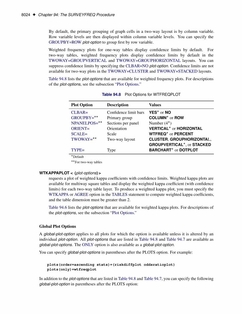
8024 F Chapter 94: The SURVEYFREQ Procedure
By default, the primary grouping of graph cells in a two-way layout is by column variable.Row variable levels are then displayed within column variable levels. You can specify theGROUPBY=ROW plot-option to group first by row variable.
Weighted frequency plots for one-way tables display confidence limits by default. Fortwo-way tables, weighted frequency plots display confidence limits by default in theTWOWAY=GROUPVERTICAL and TWOWAY=GROUPHORIZONTAL layouts. You cansuppress confidence limits by specifying the CLBAR=NO plot-option. Confidence limits are notavailable for two-way plots in the TWOWAY=CLUSTER and TWOWAY=STACKED layouts.
Table 94.8 lists the plot-options that are available for weighted frequency plots. For descriptionsof the plot-options, see the subsection “Plot Options.”
Table 94.8 Plot Options for WTFREQPLOT
Plot Option Description Values
CLBAR= Confidence limit bars YES� or NOGROUPBY=�� Primary group COLUMN� or ROWNPANELPOS=�� Sections per panel Number (4�)ORIENT= Orientation VERTICAL� or HORIZONTALSCALE= Scale WTFREQ� or PERCENTTWOWAY=�� Two-way layout CLUSTER, GROUPHORIZONTAL,
GROUPVERTICAL�, or STACKEDTYPE= Type BARCHART� or DOTPLOT�Default��For two-way tables
WTKAPPAPLOT < (plot-options) >requests a plot of weighted kappa coefficients with confidence limits. Weighted kappa plots areavailable for multiway square tables and display the weighted kappa coefficient (with confidencelimits) for each two-way table layer. To produce a weighted kappa plot, you must specify theWTKAPPA or AGREE option in the TABLES statement to compute weighted kappa coefficients,and the table dimension must be greater than 2.
Table 94.6 lists the plot-options that are available for weighted kappa plots. For descriptions ofthe plot-options, see the subsection “Plot Options.”
Global Plot Options
A global-plot-option applies to all plots for which the option is available unless it is altered by anindividual plot-option. All plot-options that are listed in Table 94.8 and Table 94.7 are available asglobal-plot-options. The ONLY option is also available as a global-plot-option.
You can specify global-plot-options in parentheses after the PLOTS option. For example:
plots(order=ascending stats)=(riskdiffplot oddsratioplot)plots(only)=wtfreqplot
In addition to the plot-options that are listed in Table 94.8 and Table 94.7, you can specify the followingglobal-plot-option in parentheses after the PLOTS option:

TABLES Statement F 8025
ONLYsuppresses the default plots and requests only the plots that are specified as plot-requests.
Plot Options
You can specify the following plot-options in parentheses after a plot-request .
CLBAR=NO | YEScontrols the confidence limit error bars in weighted frequency plots (WTFREQPLOT). By default,CLBAR=YES, which displays confidence limits error bars; CLBAR=NO suppresses confidencelimit error bars.
This plot-option applies to all weighted frequency plots except those two-way plots that aredisplayed in the TWOWAY=CLUSTER or TWOWAY=STACKED layout. Confidence limit errorbars are not available in the TWOWAY=CLUSTER and TWOWAY=STACKED layouts.
CLDISPLAY=SERIF | SERIFARROW | LINE | LINEARROW | BAR < width >controls the appearance of the confidence limit error bars. This plot-option is available for thefollowing plots: KAPPAPLOT, ODDSRATIOPLOT, RELRISKPLOT, RISKDIFFPLOT, andWTKAPPAPLOT.
The default is CLDISPLAY=SERIF, which displays the confidence limits as lines with serifs.CLDISPLAY=LINE displays the confidence limits as plain lines without serifs. The CLDIS-PLAY=SERIFARROW and CLDISPLAY=LINEARROW plot-options display arrowheads onany error bars that are clipped by the RANGE= plot-option; if an entire error bar is cut from theplot, the plot displays an arrowhead that points toward the statistic.
CLDISPLAY=BAR displays the confidence limits as bars. By default, the width of the barsequals the size of the marker for the estimate. You can control the width of the bars and thesize of the marker by specifying the value of width as a percentage of the distance between bars,0 < width � 1. The bar might disappear when the value of width is very small.
COLUMN=1 | 2specifies the 2�2 table column to use to compute the risk (proportion). This plot-option is availablefor the relative risk plot (RELRISKPLOT) and the risk difference plot (RISKDIFFPLOT). Ifyou specify COLUMN=1, the plot displays the column 1 relative risks or the column 1 riskdifferences. Similarly, if you specify COLUMN=2, the plot displays the column 2 relative risksor risk differences.
For relative risk plots, the default is COLUMN=1. For risk difference plots, the default ifCOLUMN=1 if you request computation of both column 1 and column 2 risk differenceswith the RISK option. If you request computation of only column 1 (or only column 2) riskdifferences with the RISK1 (or RISK2) option, by default the risk difference plot displays theserisk differences.
GROUPBY=COLUMN | ROWspecifies the primary grouping for two-way weighted frequency plots, which you can request byspecifying the WTFREQPLOT plot-request .
The default is GROUPBY=COLUMN, which groups graph cells first by column variable anddisplays row variable levels within column variable levels. You can specify GROUPBY=ROW to

8026 F Chapter 94: The SURVEYFREQ Procedure
group first by row variable. In two-way and multiway table requests, the column variable is thelast variable specified and forms the columns of the crosstabulation table. The row variable is thenext-to-last variable specified and forms the rows of the table.
By default for a bar chart that is displayed in the TWOWAY=STACKED layout, bars correspondto the column variable levels and row levels are displayed (stacked) within each column bar.By default for a bar chart that is displayed in the TWOWAY=CLUSTER layout, bars are firstgrouped by column variable levels, and row levels are displayed as adjacent bars within eachcolumn-level group. You can reverse the default row and column variable groupings by specifyingGROUPBY=ROW.
LOGBASE=2 | E | 10applies to the odds ratio plot (ODDSRATIOPLOT) and the relative risk plot (RELRISKPLOT).This plot-option displays the odds ratio or relative risk axis on the log scale that you specify.
NPANELPOS=ndivides the plot into multiple panels that display at most jnj statistics or sections.
If n is positive, the number of statistics or sections per panel is balanced; if n is negative, thenumber of statistics per panel is not balanced. For example, suppose you want to display 21 oddsratios. NPANELPOS=20 displays two panels, the first with 11 odds ratios and the second with10 odds ratios; NPANELPOS=–20 displays 20 odds ratios in the first panel but only 1 in thesecond panel. This plot-option is available for all plots except mosaic plots and one-way weightedfrequency plots.
For two-way weighted frequency plots (WTFREQPLOT), NPANELPOS=n requests that pan-els display at most jnj sections, where sections correspond to row or column variable lev-els, depending on the type of plot and the grouping. By default, n=4 and each panelincludes at most four sections. This plot-option applies to two-way plots that are dis-played in the TWOWAY=GROUPVERTICAL or TWOWAY=GROUPHORIZONTAL lay-out. The NPANELPOS= plot-option does not apply to the TWOWAY=CLUSTER andTWOWAY=STACKED layouts, which are always displayed in a single panel.
For plots that display statistics with confidence limits, NPANELPOS=n requests that panelsdisplay at most jnj statistics. By default, n=0 and all statistics are displayed in a single panel. Thisplot-option applies to the following plots: KAPPAPLOT, ODDSRATIOPLOT, RELRISKPLOT,RISKDIFFPLOT, and WTKAPPAPLOT.
ORDER=ASCENDING | DESCENDINGdisplays the two-way table (layer) statistics in order of the statistic value. If you specify OR-DER=ASCENDING or ORDER=DESCENDING, the plot displays the statistics in ascending ordescending order, respectively. By default, the order of the statistics in the plot matches the orderthat the two-way table layers appear in the multiway table.
This plot-option is available for the following plots: KAPPAPLOT, ODDSRATIOPLOT, REL-RISKPLOT, RISKDIFFPLOT, and WTKAPPAPLOT.
ORIENT=HORIZONTAL | VERTICALcontrols the orientation of weighted frequency plots (WTFREQPLOT). This plot-option placesthe variable levels on the Y axis and the weighted frequencies or percentages on the X axis.ORIENT=VERTICAL places the variable levels on the X axis. The default orientation is

TABLES Statement F 8027
ORIENT=VERTICAL for bar charts (TYPE=BARCHART) and ORIENT=HORIZONTAL fordot plots (TYPE=DOTPLOT).
RANGE=(< min > < , max > )| CLIPspecifies the range of values to display. If you specify RANGE=CLIP, the confidence limitsare clipped and the display range is determined by the minimum and maximum values of theestimates. By default, the display range includes all confidence limits.
This plot-option is available for the following plots: KAPPAPLOT, ODDSRATIOPLOT, REL-RISKPLOT, RISKDIFFPLOT, and WTKAPPAPLOT.
SCALE=WTFREQ | PERCENTspecifies the scale of the frequencies in weighted frequency plots (WTFREQPLOT).SCALE=WTFREQ displays weighted frequencies (totals), and SCALE=PERCENT displayspercentages. The default scale is SCALE=WTFREQ.
STATSdisplays the values of the statistics and their confidence limits on the right side of the plot. If youdo not specify this plot-option, the statistic values are not displayed.
This plot-option is available for the following plots: KAPPAPLOT, ODDSRATIOPLOT, REL-RISKPLOT, RISKDIFFPLOT, and WTKAPPAPLOT.
TWOWAY=CLUSTER | GROUPHORIZONTAL | GROUPVERTICAL | STACKEDspecifies the layout for two-way weighted frequency plots (WTFREQPLOT).
All TWOWAY= layouts are available for bar charts (TYPE=BARCHART). All TWOWAY=layouts except TWOWAY=CLUSTER are available for dot plots (TYPE=DOTPLOT). Confidencelimits (CLBAR=) can be displayed in the GROUPVERTICAL and GROUPHORIZONTALlayouts. Confidence limits are not available in the STACKED and CLUSTER layouts. TheORIENT= and GROUPBY= plot-options are available for all TWOWAY= layouts.
The default two-way layout is TWOWAY=GROUPVERTICAL, which produces a groupedplot that has a vertical common baseline. By default for bar charts (TYPE=BARCHART,ORIENT=VERTICAL), the X axis displays column variable levels, and the Y axis displaysweighted frequencies. The plot includes a vertical (Y-axis) block for each row variable level. Therelative positions of the graph cells in this plot layout are the same as the relative positions of thetable cells in the crosstabulation table. You can reverse the default row and column grouping byspecifying the GROUPBY=ROW plot-option.
The TWOWAY=GROUPHORIZONTAL layout produces a grouped plot that has a horizontalcommon baseline. By default (GROUPBY=COLUMN), the plot displays a block on the X axisfor each column variable level. Within each column-level block, the plot displays row variablelevels.
The TWOWAY=STACKED layout produces stacked displays of weighted frequencies. By default(GROUPBY=COLUMN) in a stacked bar chart, the bars correspond to column variable levels,and row levels are stacked within each column level. By default in a stacked dot plot, the dottedlines correspond to column levels, and cell weighted frequencies are plotted as data dots on thecorresponding column line. The dot color identifies the row level.
The TWOWAY=CLUSTER layout, which is available only for bar charts, displays groups ofadjacent bars. By default, the primary grouping is by column variable level, and row levels aredisplayed within each column level.

8028 F Chapter 94: The SURVEYFREQ Procedure
You can reverse the default row and column grouping in any layout by specifying theGROUPBY=ROW plot-option. The default is GROUPBY=COLUMN, which groups first bycolumn variable.
TYPE=BARCHART | DOTPLOTspecifies the type (form) of the weighted frequency plots (WTFREQPLOT). TYPE=BARCHARTproduces a bar chart and TYPE=DOTPLOT produces a dot plot. The default type isTYPE=BARCHART.
RISK
RISKDIFFrequests risk statistics for 2 � 2 tables. The RISK option also provides standard errors and confidencelimits for these statistics. Risk statistics include the row 1 risk (proportion), row 2 risk, overall risk,and risk difference. See the section “Risks and Risk Difference” on page 8054 for details.
The RISK option provides both column 1 and column 2 risks. To request only column 1 or column 2risks, use the RISK1 or RISK2 option.
To compute confidence limits for the risks and risk difference, PROC SURVEYFREQ determines theconfidence coefficient from the ALPHA= option, which by default equals 0.05 and produces 95%confidence limits.
RISK1
RISKDIFF1requests column 1 risk statistics for 2 � 2 tables, together with their standard errors and confidencelimits. Risk statistics include the row 1 risk (proportion), row 2 risk, overall risk, and risk difference.See the section “Risks and Risk Difference” on page 8054 for details.
To compute confidence limits for the risks and risk difference, PROC SURVEYFREQ determines theconfidence coefficient from the ALPHA= option, which by default equals 0.05 and produces 95%confidence limits.
RISK2
RISKDIFF2requests column 2 risk statistics for 2 � 2 tables, together with their standard errors and confidencelimits. Risk statistics include the row 1 risk (proportion), row 2 risk, overall risk, and risk difference.See the section “Risks and Risk Difference” on page 8054 for details.
To compute confidence limits for the risks and risk difference, PROC SURVEYFREQ determines theconfidence coefficient from the ALPHA= option, which by default equals 0.05 and produces 95%confidence limits.
ROW < (option) >displays the row percentage (estimated proportion of the row total) for each cell in a two-way table.The ROW option also provides the standard errors of the row percentages. See the section “Row andColumn Proportions” on page 8042 for more information. This option has no effect for one-way tables.
You can specify the following option:
DEFFdisplays the design effect for each row percentage in the crosstabulation table. See the section“Design Effect” on page 8052 for more information.

TABLES Statement F 8029
TESTP=(values)specifies null hypothesis proportions (test percentages) for chi-square tests for one-way tables(goodness-of-fit tests). You can separate values with blanks or commas. Specify values in probabilityform as numbers between 0 and 1, where the proportions sum to 1. Or specify values in percentageform as numbers between 0 and 100, where the percentages sum to 100. PROC SURVEYFREQ treatsthe value 1 as the percentage form 1%. The number of TESTP= values must equal the number ofvariable levels in the one-way table. List these values in the same order in which the correspondingvariable levels appear in the output.
When you specify the TESTP= option, PROC SURVEYFREQ displays the specified test percentagesin the one-way frequency table. The TESTP= option has no effect for two-way tables.
PROC SURVEYFREQ uses the TESTP= values for the one-way Rao-Scott chi-square test (CHISQ)and for the one-way Rao-Scott likelihood ratio chi-square test (LRCHISQ). See the sections “Rao-ScottChi-Square Test” on page 8060 and “Rao-Scott Likelihood Ratio Chi-Square Test” on page 8065 fordetails.
VARdisplays the variance estimate for each percentage in the crosstabulation table. See the section“Proportions” on page 8040 for details. By default, PROC SURVEYFREQ displays the standard errorsof the percentages.
VARWTdisplays the variance estimate for each weighted frequency, or estimated total, in the crosstabulationtable. See the section “Totals” on page 8038 for details. By default, PROC SURVEYFREQ displaysthe standard deviations of the weighted frequencies.
WCHISQrequests the Wald chi-square test for two-way tables. See the section “Wald Chi-Square Test” onpage 8067 for details.
WLLCHISQrequests the Wald log-linear chi-square test for two-way tables. See the section “Wald Log-LinearChi-Square Test” on page 8068 for details.
WTFREQdisplays totals (weighted frequencies) and their standard errors when you do not specify a WEIGHTor REPWEIGHTS statement. PROC SURVEYFREQ displays the weighted frequencies by defaultwhen you include a WEIGHT or REPWEIGHTS statement. Without a WEIGHT or REPWEIGHTSstatement, PROC SURVEYFREQ assigns all observations a weight of one.
WTKAPPA < (options) >requests the weighted kappa coefficient with its standard error and confidence limits. Weighted kappacoefficients can be computed for square two-way tables, where the number of rows equals the numberof columns. For 2 � 2 tables, the weighted kappa coefficient equals the simple kappa coefficient, andPROC SURVEYFREQ displays only the simple kappa coefficient. For more information, see thesection “Weighted Kappa Coefficient” on page 8058.
Weighted kappa coefficients are available when you specify variance estimation by the jackknife method(VARMETHOD=JACKKNIFE) or by balanced repeated replication (VARMETHOD=BRR); weightedkappa coefficients are not available with the Taylor series method (VARMETHOD=TAYLOR).

8030 F Chapter 94: The SURVEYFREQ Procedure
The weighted kappa coefficient is computed by using agreement weights that reflect the relativeagreement between pairs of variable levels. Agreement weights are not the same as sampling weights,which you provide by specifying the WEIGHT statement. PROC SURVEYFREQ uses the samplingweights to compute both the simple kappa and weighted kappa coefficients. For more information, seethe section “Weighted Kappa Coefficient” on page 8058.
To compute confidence limits for the weighted kappa coefficient, PROC SURVEYFREQ determinesthe confidence coefficient from the ALPHA= option, which by default equals 0.05 and produces 95%confidence limits.
You can specify the following options:
PRINTKWTSdisplays the agreement weights that PROC SURVEYFREQ uses to compute the weighted kappacoefficient. Agreement weights reflect the relative agreement between pairs of variable levels. Bydefault, PROC SURVEYFREQ computes these weights by using the Cicchetti-Allison form. Ifyou specify the WT=FC option, the procedure uses the Fleiss-Cohen form of agreement weights.For more information, see the section “Weighted Kappa Coefficient” on page 8058.
WT=FCrequests Fleiss-Cohen agreement weights for the weighted kappa computation. By default,PROC SURVEYFREQ uses Cicchetti-Allison agreement weights to compute the weighted kappacoefficient. Agreement weights reflect the relative agreement between pairs of variable levels.For more information, see the section “Weighted Kappa Coefficient” on page 8058.
WEIGHT StatementWEIGHT variable ;
The WEIGHT statement names the variable that contains the sampling weights. This variable must be numeric,and the sampling weights must be positive numbers. If an observation has a weight that is nonpositive ormissing, then the procedure omits that observation from the analysis. See the section “Missing Values” onpage 8033 for more information. If you specify more than one WEIGHT statement, the procedure uses onlythe first WEIGHT statement and ignores the rest.
If you do not specify a WEIGHT statement but provide replicate weights with a REPWEIGHTS statement,PROC SURVEYFREQ uses the average of each observation’s replicate weights as the observation’s weight.
If you do not specify a WEIGHT statement or a REPWEIGHTS statement, PROC SURVEYFREQ assignsall observations a weight of one.

Details: SURVEYFREQ Procedure F 8031
Details: SURVEYFREQ Procedure
Specifying the Sample DesignPROC SURVEYFREQ produces tables and statistics that are based on the sample design used to obtain thesurvey data. PROC SURVEYFREQ can be used for single-stage or multistage designs, with or without strati-fication, and with or without unequal weighting. To analyze your survey data with PROC SURVEYFREQ,you need to provide sample design information for the procedure. This information can include design strata,clusters, and sampling weights. You can provide sample design information with the STRATA, CLUSTER,and WEIGHT statements, and with the RATE= or TOTAL= option in the PROC SURVEYFREQ statement.
If you provide replicate weights for BRR or jackknife variance estimation, you do not need to specify aSTRATA or CLUSTER statement. Otherwise, you should specify STRATA and CLUSTER statementswhenever your design includes stratification and clustering.
When there are clusters (PSUs) in the sample design, the procedure estimates variance by using the PSUs,as described in the section “Statistical Computations” on page 8036. For a multistage sample design, thevariance estimation depends only on the first stage of the sample design. Therefore, the required inputincludes only first-stage cluster (PSU) and first-stage stratum identification. You do not need to input designinformation about any additional stages of sampling.
Stratification
If your sample design is stratified at the first stage of sampling, use the STRATA statement to name thevariables that form the strata. The combinations of categories of STRATA variables define the strata in thesample, where strata are nonoverlapping subgroups that were sampled independently. If your sample designhas stratification at multiple stages, you should identify only the first-stage strata in the STRATA statement.
If you use a REPWEIGHTS statement to provide replicate weights for BRR or jackknife variance estimation,you do not need to specify a STRATA statement. Otherwise, you should specify a STRATA statementwhenever your design includes stratification. If you do not specify a STRATA statement or a REPWEIGHTSstatement, then PROC SURVEYFREQ assumes there is no stratification at the first stage.
Clustering
If your sample design selects clusters at the first stage of sampling, use the CLUSTER statement to namethe variables that identify the first-stage clusters, which are also called primary sampling units (PSUs). Thecombinations of categories of CLUSTER variables define the clusters in the sample. If there is a STRATAstatement, clusters are nested within strata. If your sample design has clustering at multiple stages, you shouldspecify only the first-stage clusters (PSUs) in the CLUSTER statement. PROC SURVEYFREQ assumes thateach cluster that is defined by the CLUSTER statement variables represents a PSU in the sample, and thateach observation belongs to one PSU.
If you use a REPWEIGHTS statement to provide replicate weights for BRR or jackknife variance estimation,you do not need to specify a CLUSTER statement. Otherwise, you should specify a CLUSTER statementwhenever your design includes clustering at the first stage of sampling. If you do not specify a CLUSTERstatement, then PROC SURVEYFREQ treats each observation as a PSU.

8032 F Chapter 94: The SURVEYFREQ Procedure
Weighting
If your sample design includes unequal weighting, use the WEIGHT statement to name the variable thatcontains the sampling weights. Sampling weights must be positive numbers. If an observation has a weightthat is nonpositive or missing, then the procedure omits that observation from the analysis. See the section“Missing Values” on page 8033 for more information.
If you do not specify a WEIGHT statement but include a REPWEIGHTS statement, PROC SURVEYFREQuses the average of each observation’s replicate weights as the observation’s weight. If you do not specify aWEIGHT statement or a REPWEIGHTS statement, PROC SURVEYFREQ assigns all observations a weightof one.
Population Totals and Sampling Rates
To include a finite population correction (fpc) in Taylor series variance estimation, you can input either thesampling rate or the population total by using the RATE= or TOTAL= option in the PROC SURVEYFREQstatement. (You cannot specify both of these options in the same PROC SURVEYFREQ statement.) TheRATE= and TOTAL= options apply only to Taylor series variance estimation. The procedure does not use afinite population correction for BRR or jackknife variance estimation.
If you do not specify the RATE= or TOTAL= option, Taylor series variance estimation does not include afinite population correction. For fairly small sampling fractions, it is appropriate to ignore this correction.See Cochran (1977) and Kish (1965) for more information.
If your design has multiple stages of selection and you are specifying the RATE= option, you should inputthe first-stage sampling rate, which is the ratio of the number of PSUs in the sample to the total number ofPSUs in the study population. If you are specifying the TOTAL= option for a multistage design, you shouldinput the total number of PSUs in the study population.
For a nonstratified sample design, or for a stratified sample design with the same sampling rate or the samepopulation total in all strata, you can use the RATE=value or TOTAL=value option. If your sample design isstratified with different sampling rates or population totals in different strata, use the RATE=SAS-data-set orTOTAL=SAS-data-set option to name a SAS data set that contains the stratum sampling rates or totals. Thisdata set is called a secondary data set, as opposed to the primary data set that you specify with the DATA=option.
The secondary data set must contain all the stratification variables listed in the STRATA statement andall the variables in the BY statement. Furthermore, the BY groups must appear in the same order asin the primary data set. If there are formats that are associated with the STRATA variables and the BYvariables, then the formats must be consistent in the primary and the secondary data sets. If you specify theTOTAL=SAS-data-set option, the secondary data set must have a variable named _TOTAL_ that contains thestratum population totals. If you specify the RATE=SAS-data-set option, the secondary data set must have avariable named _RATE_ that contains the stratum sampling rates. If the secondary data set contains morethan one observation for any one stratum, the procedure uses the first value of _TOTAL_ or _RATE_ for thatstratum and ignores the rest.
The value in the RATE= option or the values of _RATE_ in the secondary data set must be nonnegativenumbers. You can specify value as a number between 0 and 1. Or you can specify value in percentageform as a number between 1 and 100, and PROC SURVEYFREQ converts that number to a proportion. Theprocedure treats the value 1 as 100% instead of 1%.

Domain Analysis F 8033
If you specify the TOTAL=value option, value must not be less than the sample size. If you provide stratumpopulation totals in a secondary data set, these values must not be less than the corresponding stratum samplesizes.
Domain AnalysisPROC SURVEYFREQ provides domain analysis through its multiway table capability. Domain analysisrefers to the computation of statistics for domains (subpopulations), in addition to the computation of statisticsfor the entire study population. Formation of subpopulations can be unrelated to the sample design, and sothe domain sample sizes can actually be random variables. Domain analysis takes this variability into accountby using the entire sample in estimating the variance of domain estimates. Domain analysis is also known assubgroup analysis, subpopulation analysis, and subdomain analysis. For more information about domainanalysis, see Lohr (2010); Cochran (1977); Fuller et al. (1989).
To request domain analysis with PROC SURVEYFREQ, you should include the domain variable(s) in yourTABLES statement request. For example, specifying DOMAIN * A * B in a TABLES statement producesseparate two-way tables of A by B for each level of DOMAIN. If your domains are formed by more than onevariable, you can specify DomainVariable_1 * DomainVariable_2 * A * B, for example, to obtain two-waytables of A by B for each domain formed by the different combinations of levels for DomainVariable_1 andDomainVariable_2. See Example 94.2 for an example of domain analysis.
If you specify DOMAIN * A in a TABLES statement, the values of the variable DOMAIN form the table rows.The two-way table lists levels of the variable A within each level of the row variable DOMAIN. Specify theROW option in the TABLES statement to obtain the row percentages and their standard errors. This providesthe one-way distribution of A for each domain (level of the variable DOMAIN).
Including the domain variables in a TABLES statement request provides a different analysis from thatobtained by using a BY statement, which provides completely separate analyses of the BY groups. TheBY statement can also be used to analyze the data set by subgroups, but it is critical to note that this doesnot produce a valid domain analysis. The BY statement is appropriate only when the number of units ineach subgroup is known with certainty. For example, the BY statement can be used to obtain stratum levelestimates when you have fixed sample sizes for the strata. When the subgroup sample size is a randomvariable, include the domain variables in your TABLES statement request.
Missing Values
WEIGHT Variable
If an observation has a missing value or a nonpositive value for the WEIGHT variable, then PROCSURVEYFREQ excludes that observation from the analysis.
REPWEIGHTS Variables
If you provide replicate weights with a REPWEIGHTS statement for BRR or jackknife variance estimation,all REPWEIGHTS variable values must be nonmissing. Similarly, if you provide jackknife coefficients withthe JKCOEFS= option in the REPWEIGHTS statement, all values of the JKCoefficient variable must benonmissing. The procedure does not perform the analysis when any replicate weight or jackknife coefficientvalue is missing.

8034 F Chapter 94: The SURVEYFREQ Procedure
STRATA and CLUSTER Variables
An observation is excluded from the analysis if it has a missing value for any STRATA or CLUSTER variable,unless you specify the MISSING option in the PROC SURVEYFREQ statement. If you specify the MISSINGoption, the procedure treats missing values as a valid (nonmissing) category for all categorical variables,which include STRATA variables, CLUSTER variables, and TABLES variables.
TABLES Variables
By default, PROC SURVEYFREQ excludes an observation from a crosstabulation table (and all associatedanalyses) if the observation has a missing value for any of the variables in the TABLES request, unless youspecify the MISSING or NOMCAR option in the PROC SURVEYFREQ statement. When the procedureexcludes observations with missing values from a table, it displays the total frequency of missing observationsbelow the table.
If you specify the MISSING option, the procedure treats missing values as a valid (nonmissing) level foreach TABLES variable. These levels are displayed in the crosstabulation table and included in computationsof totals, percentages, and all other table statistics.
If you specify the NOMCAR option in the PROC SURVEYFREQ statement for Taylor series varianceestimation, the procedure includes observations with missing values of TABLES variables in the variancecomputations. The NOMCAR option does not display missing levels in the crosstabulation table or computepercentages and totals for missing levels.
The NOMCAR Option
The NOMCAR option in the PROC SURVEYFREQ statement includes observations with missing values ofTABLES variables in the variance computations as not missing completely at random (NOMCAR) for Taylorseries variance estimation. By default, observations are completely excluded from the analysis if they havemissing values for any of the variables in the current TABLES request. This default treatment is based on theassumption that the values are missing completely at random (MCAR), and assumes that the analysis resultsshould not be substantially different between the missing and nonmissing groups. See the section “AnalysisConsiderations” on page 8036 for more information.
When you specify the NOMCAR option, PROC SURVEYFREQ computes variance estimates by analyzingthe nonmissing values as a domain (subpopulation), where the entire population includes both nonmissingand missing domains.
The NOMCAR option has no effect when you specify the MISSING option, which treats missing values as avalid nonmissing level. The NOMCAR option does not affect the inclusion of observations with missingvalues of the WEIGHT, CLUSTER, or STRATA variables. Observations with missing values of the WEIGHTvariable are always excluded from the analysis. Observations with missing values of the CLUSTER orSTRATA variables are excluded unless you specify the MISSING option.
The NOMCAR option applies only to Taylor series variance estimation VARMETHOD=TAYLOR. Thereplication methods, which you request with the VARMETHOD=BRR and VARMETHOD=JACKKNIFEoptions, do not use the NOMCAR option.

Missing Values F 8035
Degrees of Freedom
PROC SURVEYFREQ computes the degrees of freedom to obtain the t-percentile for confidence limits forproportions, totals, and other statistics. The procedure also uses the degrees of freedom for the F statisticsin the Rao-Scott and Wald chi-square tests. The degrees of freedom computation depends on the sampledesign and the variance estimation method. For more information, see the section “Degrees of Freedom” onpage 8051. Missing values can affect the degrees of freedom computation.
Taylor Series Variance EstimationThe degrees of freedom can depend on the number of clusters, the number of strata, and the number ofobservations. For Taylor series variance estimation, these numbers are based on the observations included inthe analysis of the individual table. These numbers do not count observations that are excluded from the tabledue to missing values. If all values in a stratum are excluded from the analysis of a table as missing values,then that stratum is called an empty stratum. Empty strata are not counted in the total number of strata for thetable. Similarly, empty clusters and missing observations are not included in the total counts of clusters andobservations that are used to compute the degrees of freedom for the analysis.
If you specify the MISSING option, missing values are treated as valid nonmissing levels and are included incomputing degrees of freedom. If you specify the NOMCAR option for Taylor series variance estimation,observations with missing values of the TABLES variables are included in computing degrees of freedom.
Replicate-Based Variance EstimationFor BRR or jackknife variance estimation, by default PROC SURVEYFREQ computes the degrees offreedom by using all valid observations in the input data set. A valid observation is an observation that has apositive value of the WEIGHT variable and nonmissing values of the STRATA and CLUSTER variablesunless you specify the MISSING option. See the section “Data Summary Table” on page 8070 for detailsabout valid observations.
If you specify the DFADJ method-option for VARMETHOD=BRR or VARMETHOD=JACKKNIFE, theprocedure computes the degrees of freedom based on the nonmissing observations included in the individualtable request. This excludes any empty strata or clusters that occur when observations with missing values ofthe TABLES variables are removed from the analysis for that table.
Table Summary Output Data Set
For each table request, PROC SURVEYFREQ produces a nondisplayed ODS table, “Table Summary,” whichcontains the number of (nonmissing) observations, strata, and clusters that are included in the analysis ofthe individual table. If there are missing observations, empty strata, or empty clusters excluded from theanalysis, the “Table Summary” data set also contains this information. If you request any confidence limits orchi-square tests for the table, which require degrees of freedom, the “Table Summary” data set provides thedegrees of freedom.
Due to missing values, the number of observations used for an individual table analysis can differ from thenumber of valid observations in the input data set, which is reported in the “Data Summary” table. Similarly,a difference can also occur for the number of clusters or strata. See Example 94.3 for more information aboutthe “Table Summary” output data set.
If you specify the NOMCAR option for Taylor series variance estimation, the “Table Summary” data setreflects all observations used for variance estimation, which includes those observations with missing valuesof the TABLES variables.

8036 F Chapter 94: The SURVEYFREQ Procedure
Analysis Considerations
If you have missing values in your survey data for any reason (such as nonresponse), this can compromise thequality of your survey results. An observation without missing values is called a complete respondent, and anobservation with missing values is called an incomplete respondent. If the complete respondents are differentfrom the incomplete respondents with regard to a survey effect or outcome, then survey estimates will bebiased and will not accurately represent the survey population. There are a variety of techniques in sampledesign and survey operations that can reduce nonresponse. After data collection is complete, you can useimputation to replace missing values with acceptable values, and you can use sampling weight adjustments tocompensate for nonresponse. You should complete this data preparation and adjustment before you analyzeyour data with PROC SURVEYFREQ. For more details, see Cochran (1977); Kalton and Kasprzyk (1986);Brick and Kalton (1996).
Statistical Computations
Variance Estimation
PROC SURVEYFREQ provides a choice of variance estimation methods for complex survey data. In additionto the Taylor series linearization method, the procedures offer two replication-based (resampling) methods—balanced repeated replication (BRR) and the delete-1 jackknife. These variance estimation methods usuallygive similar, satisfactory results (Lohr 2010; Särndal, Swensson, and Wretman 1992; Wolter 1985). Thechoice of a variance estimation method can depend on the sample design used, the sample design informationavailable, the parameters to be estimated, and computational issues. See Lohr (2010) for more details.
Taylor Series Variance EstimationThe Taylor series linearization method can be used to estimate standard errors of proportions and otherstatistics for crosstabulation tables. For sample survey data, the proportion estimator is a ratio estimatorformed from estimators of totals. For example, to estimate the proportion in a crosstabulation table cell, theprocedure uses the ratio of the estimator of the cell total frequency to the estimator of the overall populationtotal, where these totals are linear statistics computed from the survey data. The Taylor series expansionmethod obtains a first-order linear approximation for the ratio estimator and then uses the variance estimatefor this approximation to estimate the variance of the estimate itself (Woodruff 1971; Fuller 1975). Formore information about Taylor series variance estimation for sample survey data, see Lohr (2010); Särndal,Swensson, and Wretman (1992); Lee, Forthofer, and Lorimor (1989); Wolter (1985).
When there are clusters (PSUs) in the sample design, the Taylor series method estimates variance from thevariance among PSUs. When the design is stratified, the procedure combines stratum variance estimatesto compute the overall variance estimate. For a multistage sample design, the variance estimation dependsonly on the first stage of the sample design. So the required input includes only first-stage cluster (PSU) andfirst-stage stratum identification. You do not need to input design information about any additional stages ofsampling. This variance estimation method assumes that the first-stage sampling fraction is small, or thefirst-stage sample is drawn with replacement, as it often is in practice.
See the sections “Proportions” on page 8040, “Row and Column Proportions” on page 8042, “Risks and RiskDifference” on page 8054, and “Odds Ratio and Relative Risks” on page 8055 for details and formulas forTaylor series variance estimates.

Statistical Computations F 8037
Replication-Based Variance EstimationReplication-based methods for variance estimation draw multiple replicates (subsamples) from the fullsample by following a specific resampling scheme. Commonly used resampling schemes include balancedrepeated replication (BRR) and the jackknife. PROC SURVEYFREQ estimates the parameter of interest(a proportion, total, odds ratio, or other statistic) from each replicate, and then uses the variability amongreplicate estimates to estimate the overall variance of the parameter estimate. See Wolter (1985) and Lohr(2010) for more information.
The BRR variance estimation method requires a stratified sample design with two PSUs in each stratum.Each replicate is obtained by deleting one PSU per stratum according to the corresponding Hadamard matrixand adjusting the original weights of the remaining PSUs. The adjusted weights are called replicate weights.PROC SURVEYFREQ also provides Fay’s method, which is a modification of the BRR method. See thesection “Balanced Repeated Replication (BRR)” on page 8043 for details.
The jackknife method deletes one PSU at a time from the full sample to create replicates, and modifies theoriginal weights to obtain replicate weights. The total number of replicates equals the number of PSUs. Ifthe sample design is stratified, each stratum must contain at least two PSUs, and the jackknife is appliedseparately within each stratum. See the section “The Jackknife Method” on page 8046 for details.
Instead of having PROC SURVEYFREQ generate replicate weights for the analysis, you can input your ownreplicate weights with a REPWEIGHTS statement. This can be useful if you need to do multiple analyseswith the same set of replicate weights, or if you have access to replicate weights instead of design information.See the section “Replicate Weight Output Data Set” on page 8069 for more information.
Definitions and Notation
For a stratified clustered sample design, define the following:
h D 1; 2; : : : ;H is the stratum number,with a total of H strata
i D 1; 2; : : : ; nh is the cluster number within stratum h,with a total of nh sample clusters in stratum h
j D 1; 2; : : : ; mhi is the unit number within cluster i of stratum h,with a total of mhi sample units from cluster i of stratum h
n DPHhD1
Pnh
iD1 mhi is the total number of observations in the sample
fh D first-stage sampling rate for stratum h
Whij D sampling weight of unit j in cluster i of stratum h
The sampling rate fh, which is used in Taylor series variance estimation, is the fraction of first-stage units(PSUs) selected for the sample. You can specify the stratum sampling rates with the RATE= option. Or ifyou specify population totals with the TOTAL= option, PROC SURVEYFREQ computes fh as the ratio ofstratum sample size to the stratum total, in terms of PSUs. See the section “Population Totals and SamplingRates” on page 8032 for details. If you do not specify the RATE= option or the TOTAL= option, then theprocedure assumes that the stratum sampling rates fh are negligible and does not use a finite populationcorrection when computing variances.
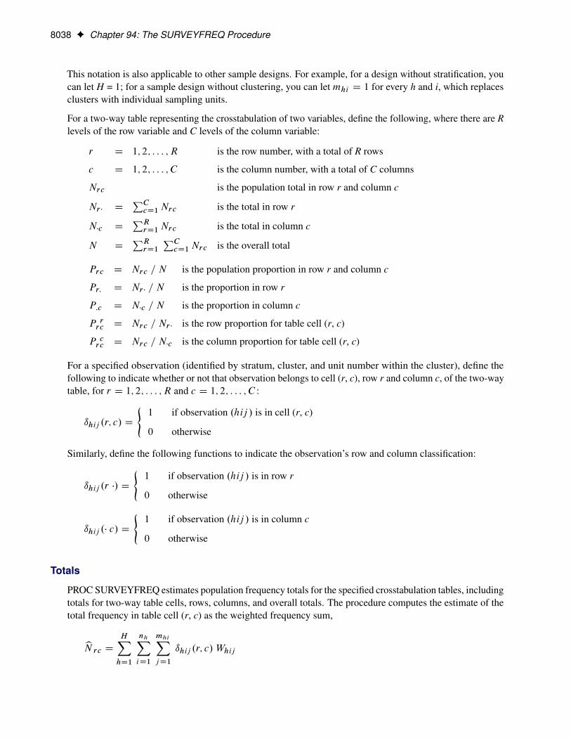
8038 F Chapter 94: The SURVEYFREQ Procedure
This notation is also applicable to other sample designs. For example, for a design without stratification, youcan let H = 1; for a sample design without clustering, you can let mhi D 1 for every h and i, which replacesclusters with individual sampling units.
For a two-way table representing the crosstabulation of two variables, define the following, where there are Rlevels of the row variable and C levels of the column variable:
r D 1; 2; : : : ; R is the row number, with a total of R rows
c D 1; 2; : : : ; C is the column number, with a total of C columns
Nrc is the population total in row r and column c
Nr � DPCcD1Nrc is the total in row r
N�c DPRrD1Nrc is the total in column c
N DPRrD1
PCcD1Nrc is the overall total
Prc D Nrc = N is the population proportion in row r and column c
Pr: D Nr � = N is the proportion in row r
P:c D N�c = N is the proportion in column c
P rrc D Nrc = Nr � is the row proportion for table cell (r, c)
P crc D Nrc = N�c is the column proportion for table cell (r, c)
For a specified observation (identified by stratum, cluster, and unit number within the cluster), define thefollowing to indicate whether or not that observation belongs to cell (r, c), row r and column c, of the two-waytable, for r D 1; 2; : : : ; R and c D 1; 2; : : : ; C :
ıhij .r; c/ D
(1 if observation .hij / is in cell (r, c)
0 otherwise
Similarly, define the following functions to indicate the observation’s row and column classification:
ıhij .r �/ D
(1 if observation .hij / is in row r
0 otherwise
ıhij .� c/ D
(1 if observation .hij / is in column c
0 otherwise
Totals
PROC SURVEYFREQ estimates population frequency totals for the specified crosstabulation tables, includingtotals for two-way table cells, rows, columns, and overall totals. The procedure computes the estimate of thetotal frequency in table cell (r, c) as the weighted frequency sum,
bN rc D
HXhD1
nhXiD1
mhiXjD1
ıhij .r; c/ Whij

Statistical Computations F 8039
Similarly, PROC SURVEYFREQ computes estimates of row totals, column totals, and overall totals as
bN r � D
HXhD1
nhXiD1
mhiXjD1
ıhij .r �/ Whij
bN �c D HXhD1
nhXiD1
mhiXjD1
ıhij .� c/ Whij
bN D
HXhD1
nhXiD1
mhiXjD1
Whij
PROC SURVEYFREQ estimates the variances of totals by using the variance estimation method that yourequest. If you request BRR variance estimation (by specifying the VARMETHOD=BRR option in the PROCSURVEYFREQ statement), the procedure estimates the variances as described in the section “BalancedRepeated Replication (BRR)” on page 8043. If you request jackknife variance estimation (by specifying theVARMETHOD=JACKKNIFE option), the procedure estimates the variances as described in the section “TheJackknife Method” on page 8046.
If you do not specify the VARMETHOD= option or a REPWEIGHTS statement, the default varianceestimation method is Taylor series, which you can also request with the VARMETHOD=TAYLOR option.Since totals are linear statistics, their variances can be estimated directly, without the approximation that isused for proportions and other nonlinear statistics. PROC SURVEYFREQ estimates the variance of the totalfrequency in table cell (r, c) as
bVar.bN rc/ D
HXhD1
bVarh.bN rc/
where if nh > 1,
bVarh.bN rc/ Dnh.1 � fh/
nh � 1
nhXiD1
.n hirc � Nnhrc/
2
n hirc D
mhiXjD1
ıhij .r; c/ Whij
Nn hrc D
nhXiD1
n hirc
!= nh
and if nh D 1,
bVarh.bN rc/ D
�missing if nh0 D 1 for h0 D 1; 2; : : : ;H0 if nh0 > 1 for some 1 � h0 � H
The standard deviation of the total is computed as
Std.bN rc/ D
qbVar.bN rc/
The variances and standard deviations are computed in a similar manner for row totals, column totals, andoverall table totals.

8040 F Chapter 94: The SURVEYFREQ Procedure
Covariance of Totals
The covariance matrix of the table cell totals bN rc is an rc � rc matrix bV.bN/, which contains the pairwisetable cell covariances bCov.bN rc ; bN ab/, for r D 1; � � � ; R; c D 1; � � � ; C ; a D 1; � � � ; R; and b D 1; � � � ; C .
PROC SURVEYFREQ estimates the covariances by using the variance estimation method that you request.If you request BRR variance estimation (by specifying the VARMETHOD=BRR option in the PROCSURVEYFREQ statement), the procedure estimates the covariances by the method described in the section“Balanced Repeated Replication (BRR)” on page 8043. If you request jackknife variance estimation (byspecifying the VARMETHOD=JACKKNIFE option), the procedure uses the method described in the section“The Jackknife Method” on page 8046.
Otherwise (by default, or if you request the Taylor series method), PROC SURVEYFREQ estimates thecovariance between total frequency estimates for table cells (r, c) and (a, b) as
bCov.bN rc ; bN ab/ D
HXhD1
nh.1 � fh/
nh � 1
nhXiD1
.n hirc � Nnhrc/ .n
hiab � Nn
hab/
!
Proportions
PROC SURVEYFREQ computes the estimate of the proportion in table cell (r, c) as the ratio of the estimatedtotal for the table cell to the estimated overall total,
bP rc D bN rc = bND
0@ HXhD1
nhXiD1
mhiXjD1
ıhij .r; c/ Whij
1A =
0@ HXhD1
nhXiD1
mhiXjD1
Whij
1AIf you request BRR variance estimation (by specifying the VARMETHOD=BRR option in the PROCSURVEYFREQ statement), the procedure estimates the variances of proportion estimates as described in thesection “Balanced Repeated Replication (BRR)” on page 8043. If you request jackknife variance estimation(by specifying the VARMETHOD=JACKKNIFE option), the procedure estimates the variances as describedin the section “The Jackknife Method” on page 8046.
If you do not specify the VARMETHOD= option or a REPWEIGHTS statement, the default varianceestimation method is Taylor series, which you can also request with the VARMETHOD=TAYLOR option.By using Taylor series linearization, the variance of a proportion estimate can be expressed as
bVar.bP rc/ D HXhD1
bVarh.bP rc/

Statistical Computations F 8041
where if nh > 1,
bVarh.bP rc/ D nh.1 � fh/
nh � 1
nhXiD1
.e hirc � Nehrc/
2
e hirc D
0@mhiXjD1
.ıhij .r; c/ � bP rc/ Whij1A = bN
Ne hrc D
nhXiD1
e hirc
!= nh
and if nh D 1,
bVarh.bP rc/ D � missing if nh0 D 1 for h0 D 1; 2; : : : ;H0 if nh0 > 1 for some 1 � h0 � H
The standard error of the proportion is computed as
StdErr.bP rc/ DqbVar.bP rc/Similarly, the estimate of the proportion in row r isbP r � D bN r � = bNAnd its variance estimate is
bVar.bP r �/ D HXhD1
bVarh.bP r �/where if nh > 1,
bVarh.bP r �/ D nh.1 � fh/
nh � 1
nhXiD1
.e hir � � Nehr � /
2
ehir � D
0@mhiXjD1
.ıhij .r �/ � bP r �/ Whij1A = bN
Nehr � D
nhXiD1
e hir �
!= nh
and if nh D 1,
bVarh.bP r �/ D � missing if nh0 D 1 for h0 D 1; 2; : : : ;H0 if nh0 > 1 for some 1 � h0 � H
The standard error of the proportion in row r is computed as
StdErr.bP r �/ DqbVar.bP r �/Computations for the proportion in column c are done in the same way.

8042 F Chapter 94: The SURVEYFREQ Procedure
Row and Column Proportions
PROC SURVEYFREQ computes the estimate of the row proportion for table cell (r, c) as the ratio of theestimated total for the table cell to the estimated total for row r,
bP rrc D
bN rc = bN r �
D
0@ HXhD1
nhXiD1
mhiXjD1
ıhij .r; c/ Whij
1A =
0@ HXhD1
nhXiD1
mhiXjD1
ıhij .r �/ Whij
1ASimilarly, PROC SURVEYFREQ estimates the column proportion for table cell (r, c) as the ratio of theestimated total for the table cell to the estimated total for column c,
bP crc D
bN rc = bN �cD
0@ HXhD1
nhXiD1
mhiXjD1
ıhij .r; c/ Whij
1A =
0@ HXhD1
nhXiD1
mhiXjD1
ıhij .� c/ Whij
1AIf you request BRR variance estimation (VARMETHOD=BRR), PROC SURVEYFREQ estimates thevariances of the row and column proportions as described in the section “Balanced Repeated Replication(BRR)” on page 8043. If you request jackknife variance estimation (VARMETHOD=JACKKNIFE), theprocedure estimates the variances as described in the section “The Jackknife Method” on page 8046.
If you do not specify the VARMETHOD= option or a REPWEIGHTS statement, the default varianceestimation method is Taylor series (VARMETHOD=TAYLOR). By using Taylor series linearization, thevariance of the row proportion estimate can be expressed as
bVar.bP rrc/ D
HXhD1
bVarh.bP rc/where if nh > 1,
bVarh.bP rrc/ D
nh.1 � fh/
nh � 1
nhXiD1
.g hirc � Nghrc/
2
g hirc D
0@mhiXjD1
.ıhij .r; c/ � bP rrc ıhij .r �// Whij
1A = bN r �
Ng hrc D
nhXiD1
g hirc
!= nh
and if nh D 1,
bVarh.bP rrc/ D
�missing if nh0 D 1 for h0 D 1; 2; : : : ;H0 if nh0 > 1 for some 1 � h0 � H

Statistical Computations F 8043
The standard error of the row proportion is computed as
StdErr.bP rrc/ D
qbVar.bP r
rc/
The Taylor series variance estimate for the column proportion is computed as described previously for therow proportion, but with
g hirc D
0@mhiXjD1
.ıhij .r; c/ � bP crc ıhij .� c// Whij
1A = bN �cBalanced Repeated Replication (BRR)
If you specify the VARMETHOD=BRR option, then PROC SURVEYFREQ uses balanced repeated repli-cation (BRR) for variance estimation. The BRR variance estimation method requires a stratified sampledesign with two PSUs in each stratum. You can provide replicate weights for BRR variance estimation byusing a REPWEIGHTS statement, or the procedure can construct replicate weights for the analysis. PROCSURVEYFREQ estimates the parameter of interest (a proportion, total, odds ratio, or other statistic) fromeach replicate, and then uses the variability among replicate estimates to estimate the overall variance of theparameter estimate. See Wolter (1985) and Lohr (2010) for more information about BRR variance estimation.
If you do not provide replicate weights with a REPWEIGHTS statement, PROC SURVEYFREQ constructsreplicates based on the stratified design with two PSUs in each stratum. This section describes replicateconstruction by the traditional BRR method. If you specify the FAY method-option for VARMETHOD=BRR,the procedure uses Fay’s modified BRR method, which is described in the section “Fay’s BRR Method” onpage 8044.
With the traditional BRR method, each replicate is obtained by deleting one PSU per stratum according tothe corresponding Hadamard matrix of dimension R, where R is the number of replicates. The number ofreplicates equals the smallest multiple of 4 that is greater than the number of strata H. Alternatively, you canspecify the number of replicates with the REPS= method-option. If a Hadamard matrix cannot be constructedfor the REPS= value that you specify, the value is increased until a Hadamard matrix of that dimension canbe constructed. Therefore, it is possible for the actual number of replicates used to be larger than the REPS=value that you specify.
You can provide a Hadamard matrix for BRR replicate construction by using the HADAMARD= method-option. Otherwise, PROC SURVEYFREQ generates an appropriate Hadamard matrix. See the section“Hadamard Matrix” on page 8045 for more information. You can display the Hadamard matrix by specifyingthe PRINTH method-option.
PROC SURVEYFREQ constructs replicates by using the first H columns of the R �R Hadamard matrix,where H denotes the number of strata. The rth replicate (r D 1; 2; : : : ; R) is drawn from the full sampleaccording to the rth row of the Hadamard matrix as follows:
• If element (r, h) of the Hadamard matrix equals 1, then the first PSU of stratum h is included in the rthreplicate, and the second PSU of stratum h is excluded.
• If element (r, h) of the Hadamard matrix equals –1, then the second PSU of stratum h is included inthe rth replicate, and the first PSU of stratum h is excluded.

8044 F Chapter 94: The SURVEYFREQ Procedure
For the PSUs included in replicate r, the original weights are doubled to form the replicate r weights. For thePSUs not included in replicate r, the replicate r weights equal zero. You can use the OUTWEIGHTS=SAS-data-set method-option to store the replicate weights in a SAS data set. See the section “Replicate WeightOutput Data Set” on page 8069 for details about the contents of the OUTWEIGHTS= data set. You canprovide these replicate weights to the procedure for subsequent analyses by using a REPWEIGHTS statement.
Let � denote the population parameter to be estimated—for example, a proportion, total, odds ratio, or otherstatistic. Let O� denote the estimate of � from the full sample, and let O�r denote the estimate from the rth BRRreplicate, which is computed by using the replicate weights. The BRR variance estimate for O� is computed as
bV . O�/ D 1
R
RXrD1
�O�r � O�
�2where R is the total number of replicates.
If a parameter cannot be estimated from some replicate(s), then the variance estimate is computed by usingthose replicates from which the parameter can be estimated. For example, suppose the parameter is a columnproportion—the proportion of column j for table cell (i, j). If a replicate r contains no observations in columnj, then the column j proportion is not estimable from replicate r. In this case, the BRR variance estimate iscomputed as
bV . O�/ D 1
R0
R0XrD1
�O�r � O�
�2where the summation is over the replicates where the parameter � is estimable, and R0 is the number of thosereplicates.
Fay’s BRR MethodIf you specify the FAY method-option for VARMETHOD=BRR, then PROC SURVEYFREQ uses Fay’sBRR method, which is a modification of the traditional BRR variance estimation method. As for traditionalBRR, Fay’s method requires a stratified sample design with two PSUs in each stratum. You can providereplicate weights by using a REPWEIGHTS statement, or the procedure can construct replicate weights forthe analysis. PROC SURVEYFREQ estimates the parameter of interest (a proportion, total, odds ratio, orother statistic) from each replicate, and then uses the variability among replicate estimates to estimate theoverall variance of the parameter estimate.
If you do not provide replicate weights with a REPWEIGHTS statement, PROC SURVEYFREQ constructsreplicates based on the stratified design with two PSUs in each stratum. As for traditional BRR, the numberof replicates R equals the smallest multiple of 4 that is greater than the number of strata H, or you can specifythe number of replicates with the REPS= method-option. You can provide a Hadamard matrix for replicateconstruction by using the HADAMARD= method-option, or PROC SURVEYFREQ generates an appropriateHadamard matrix.
The traditional BRR method constructs half-sample replicates by deleting one PSU per stratum according tothe Hadamard matrix and doubling the original weights to form replicate weights. Fay’s BRR method adjuststhe original weights by a coefficient �, where 0 � � < 1. You can specify the value of � with the FAY=method-option. If you do not specify the value of �, PROC SURVEYFREQ uses � D 0:5 by default. SeeJudkins (1990) and Rao and Shao (1999) for information about the value of the Fay coefficient. When � D 0,Fay’s method becomes the traditional BRR method. For more information, see Dippo, Fay, and Morganstein(1984); Fay (1989); Judkins (1990).

Statistical Computations F 8045
PROC SURVEYFREQ constructs Fay BRR replicates by using the first H columns of the R �R Hadamardmatrix, where H denotes the number of strata. The rth replicate (r D 1; 2; : : : ; R) is drawn from the fullsample according to the rth row of the Hadamard matrix as follows:
• If element (r, h) of the Hadamard matrix equals 1, the sampling weight of the first PSU in stratum h ismultiplied by �, and the sampling weight of the second PSU is multiplied by .2 � �/ to form the rthreplicate weights.
• If element (r, h) of the Hadamard matrix equals –1, then the sampling weight of the second PSU instratum h is multiplied by �, and the sampling weight of the first PSU is multiplied by .2 � �/ to formthe rth replicate weights.
You can use the OUTWEIGHTS= method-option to store the replicate weights in a SAS data set. See the sec-tion “Replicate Weight Output Data Set” on page 8069 for details about the contents of the OUTWEIGHTS=data set. You can provide these replicate weights to the procedure for subsequent analyses by using aREPWEIGHTS statement.
Let � denote the population parameter to be estimated—for example, a proportion, total, odds ratio, or otherstatistic. Let O� denote the estimate of � from the full sample, and let O�r denote the estimate from the rthBRR replicate, which is computed by using the replicate weights. The Fay BRR variance estimate for O� iscomputed as
bV . O�/ D 1
R.1 � �/2
RXrD1
�O�r � O�
�2where R is the total number of replicates and � is the Fay coefficient.
If you request Fay’s BRR method and also include a REPWEIGHTS statement, PROC SURVEYFREQ usesthe replicate weights that you provide and includes the Fay coefficient � in the denominator of the varianceestimate in the preceding expression.
If a parameter cannot be estimated from some replicate(s), then the variance estimate is computed by usingthose replicates from which the parameter can be estimated. For example, suppose the parameter is a columnproportion—the proportion of column j for table cell (i, j). If a replicate r contains no observations in columnj, then the column j proportion is not estimable from replicate r. In this case, the BRR variance estimate iscomputed as
bV . O�/ D 1
R0.1 � �/2
R0XrD1
�O�r � O�
�2where the summation is over the replicates where the parameter � is estimable, and R0 is the number of thosereplicates.
Hadamard MatrixPROC SURVEYFREQ uses a Hadamard matrix to construct replicates for BRR variance estimation. Youcan provide a Hadamard matrix for replicate construction by using the HADAMARD= method-option forVARMETHOD=BRR. Otherwise, PROC SURVEYFREQ generates an appropriate Hadamard matrix. Youcan display the Hadamard matrix by specifying the PRINTH method-option.

8046 F Chapter 94: The SURVEYFREQ Procedure
A Hadamard matrix A of dimension R is a square matrix that has all elements equal to 1 or –1. A Hadamardmatrix must satisfy the requirement that A0A D RI, where I is an identity matrix. The dimension of aHadamard matrix must equal 1, 2, or a multiple of 4.
For example, the following matrix is a Hadamard matrix of dimension k = 8:
1 1 1 1 1 1 1 1
1 �1 1 �1 1 �1 1 �1
1 1 �1 �1 1 1 �1 �1
1 �1 �1 1 1 �1 �1 1
1 1 1 1 �1 �1 �1 �1
1 �1 1 �1 �1 1 �1 1
1 1 �1 �1 �1 �1 1 1
1 �1 �1 1 �1 1 1 �1
For BRR replicate construction, the dimension of the Hadamard matrix must be at least H, where H denotesthe number of first-stage strata in your design. If a Hadamard matrix of a given dimension exists, it is notnecessarily unique. Therefore, if you want to use a specific Hadamard matrix, you must provide the matrix asa SAS data set in the HADAMARD=SAS-data-set method-option. You must ensure that the matrix that youprovide is actually a Hadamard matrix; PROC SURVEYFREQ does not check the validity of your Hadamardmatrix.
See the section “Balanced Repeated Replication (BRR)” on page 8043 and “Fay’s BRR Method” on page 8044for details about how the Hadamard matrix is used to construct replicates for BRR variance estimation.
The Jackknife Method
If you specify the VARMETHOD=JACKKNIFE option, PROC SURVEYFREQ uses the delete-1 jackknifemethod for variance estimation. The jackknife method can be used for stratified sample designs and fordesigns with no stratification. If your design is stratified, the jackknife method requires at least two PSUs ineach stratum. You can provide replicate weights for jackknife variance estimation by using a REPWEIGHTSstatement, or the procedure can construct replicate weights for the analysis. PROC SURVEYFREQ estimatesthe parameter of interest (a proportion, total, odds ratio, or other statistic) from each replicate, and then usesthe variability among replicate estimates to estimate the overall variance of the parameter estimate. SeeWolter (1985) and Lohr (2010) for more information about jackknife variance estimation.
If you do not provide replicate weights with a REPWEIGHTS statement, PROC SURVEYFREQ constructsthe replicates. The number of replicates R equals the number of PSUs, and the procedure deletes one PSUfrom the full sample to form each replicate. The sampling weights are modified by the jackknife coefficientfor the replicate to create the replicate weights.
If your design is not stratified (no STRATA statement), the jackknife coefficient has the same value for eachreplicate r. The jackknife coefficient equals
˛r D .R � 1/=R for r D 1; 2; : : : ; R
where R is the total number of replicates (or total number of PSUs). For the PSUs included in a replicate, thereplicate weights are computed by dividing the original sampling weights by the jackknife coefficient. Forthe deleted PSU, which is not included in the replicate, the replicate weights equal zero. The replicate weightfor the jth member of the ith PSU can be expressed as follows when the design is not stratified:
W rij D
(Wij =˛r if PSU i is included in replicate r
0 otherwise

Statistical Computations F 8047
where Wij is the original sampling weight of unit .ij /, r is the replicate number, and ˛r is the jackknifecoefficient.
If your design is stratified, the jackknife method requires at least two PSUs in each stratum. Let stratum h 0rbe the stratum from which a PSU is deleted to form the rth replicate. Stratum h 0r is called the donor stratum.The jackknife coefficients are defined as
˛r D .nh 0r� 1/=nh 0
rfor r D 1; 2; : : : ; R
where nh 0r
is the total number of PSUs in the donor stratum for replicate r. For all strata other than thedonor stratum, the replicate r weights equal the original sampling weights. For PSUs included from thedonor stratum, the replicate weights are computed by dividing the original sampling weights by the jackknifecoefficient. For the deleted PSU, which is not included in the replicate, the replicate weights equal zero. Thereplicate weight for the jth member of the ith PSU in stratum h can be expressed as
W rhij D
8̂̂<̂:̂Whij if h ¤ h 0r
Whij =˛r if h D h 0r and PSU .hi/ is included in replicate r
0 if h D h 0r and PSU .hi/ is not included in replicate r
You can use the OUTWEIGHTS= method-option to store the replicate weights in a SAS data set. You canalso use the OUTJKCOEFS= method-option to store the jackknife coefficients in a SAS data set. See thesections “Jackknife Coefficient Output Data Set” on page 8070 and “Replicate Weight Output Data Set”on page 8069 for details about the contents of these output data sets. You can provide replicate weightsand jackknife coefficients to the procedure for subsequent analyses by using a REPWEIGHTS statement.If you provide replicate weights but do not provide jackknife coefficients, PROC SURVEYFREQ uses˛r D .R � 1/=R as the jackknife coefficient for all replicates.
Let � denote the population parameter to be estimated—for example, a proportion, total, odds ratio, orother statistic. Let O� denote the estimate of � from the full sample, and let O�r be the estimate from the rthjackknife replicate, which is computed by using the replicate weights. The jackknife variance estimate for O�is computed as
bV . O�/ D RXrD1
˛r
�O�r � O�
�2where R is the total number of replicates and ˛r is the jackknife coefficient for replicate r.
If a parameter cannot be estimated from some replicate(s), then the variance estimate is computed by usingthose replicates from which the parameter can be estimated. For example, suppose the parameter is a columnproportion—the proportion of column j for table cell (i, j). If a replicate r contains no observations in columnj, then the column j proportion is not estimable from replicate r. In this case, the jackknife variance estimateis computed as
bV . O�/ D R
R0
R0XrD1
˛r
�O�r � O�
�2where the summation is over the replicates where the parameter � is estimable, and R0 is the number of thosereplicates.

8048 F Chapter 94: The SURVEYFREQ Procedure
Confidence Limits for Totals
If you specify the CLWT option in the TABLES statement, PROC SURVEYFREQ computes confidencelimits for the weighted frequencies (totals) in the crosstabulation tables.
For the total in table cell (r, c), the confidence limits are computed as
bN rc ˙
�tdf ;˛=2 � StdErr.bN rc/
�where bN rc is the estimate of the total frequency in table cell (r, c), StdErr. ONrc/ is the standard error of theestimate, and tdf ;˛=2 is the 100.1 � ˛=2/ percentile of the t distribution with df degrees of freedom. (Formore information, see the section “Degrees of Freedom” on page 8051.) The confidence level ˛ is determinedby the value of the ALPHA= option, which by default equals 0.05 and produces 95% confidence limits.
The confidence limits for row totals, column totals, and the overall total are computed similarly to theconfidence limits for table cell totals.
For each table request, PROC SURVEYFREQ produces a nondisplayed ODS table, “Table Summary,” whichcontains the number of observations, strata, and clusters that are included in the analysis of the requestedtable. When you request confidence limits, the “Table Summary” data set also contains the degrees offreedom df and the value of tdf ;˛=2 that is used to compute the confidence limits. See Example 94.3 for moreinformation about this output data set.
Confidence Limits for Proportions
If you specify the CL option in the TABLES statement, PROC SURVEYFREQ computes confidence limitsfor the proportions in the frequency and crosstabulation tables.
By default, PROC SURVEYFREQ computes Wald (“linear”) confidence limits if you do not specify analternative confidence limit type with the CL(TYPE=) option. In addition to Wald confidence limits, thefollowing types of design-based confidence limits are available for proportions: modified Clopper-Pearson(exact), modified Wilson (score), and logit confidence limits.
PROC SURVEYFREQ also provides the CL(PSMALL) option, which uses the alternative confidence limittype for extreme (small or large) proportions and uses the Wald confidence limits for all other proportions(not extreme). For the default PSMALL= value of 0.25, the procedure computes Wald confidence limits forproportions between 0.25 and 0.75 and computes the alternative confidence limit type for proportions that areoutside of this range. See Curtin et al. (2006).
For details about confidence limits for proportions based on complex survey data, including comparisons oftheir performance, see Korn and Graubard (1999, 1998); Curtin et al. (2006); Sukasih and Jang (2005). Also,in addition to the other references cited in the following sections, for information about binomial confidencelimits see Brown, Cai, and DasGupta (2001); Agresti and Coull (1998).
For each table request, PROC SURVEYFREQ produces a nondisplayed ODS table, “Table Summary,” whichcontains the number of observations, strata, and clusters that are included in the analysis of the requestedtable. When you request confidence limits, the “Table Summary” data set also contains the degrees offreedom df and the value of tdf ;˛=2 that is used to compute the confidence limits. See Example 94.3 for moreinformation about this output data set.

Statistical Computations F 8049
Wald Confidence LimitsPROC SURVEYFREQ computes standard Wald (“linear”) confidence limits for proportions by default.These confidence limits use the variance estimates that are based on the sample design. For the proportion intable cell (r, c), the Wald confidence limits are computed as
bP rc ˙ �tdf ;˛=2 � StdErr.bP rc/�where bP rc is the estimate of the proportion in table cell (r, c), StdErr.bP rc/ is the standard error of theestimate, and tdf ;˛=2 is the 100.1 � ˛=2/ percentile of the t distribution with df degrees of freedom. (Formore information, see the section “Degrees of Freedom” on page 8051.) The confidence level ˛ is determinedby the value of the ALPHA= option, which by default equals 0.05 and produces 95% confidence limits.
The confidence limits for row proportions and column proportions are computed similarly to the confidencelimits for table cell proportions.
Modified Confidence LimitsPROC SURVEYFREQ uses the modification described in Korn and Graubard (1998) to compute design-based Clopper-Pearson (exact) and Wilson (score) confidence limits. This modification substitutes thedegrees-of-freedom adjusted effective sample size for the original sample size in the confidence limitcomputations.
The effective sample size ne is computed as
ne D n = Deff
where n is the original sample size (unweighted frequency) that corresponds to the total domain of theproportion estimate, and Deff is the design effect.
If the proportion is computed for a table cell of a two-way table, then the domain is the two-way table, andthe sample size n is the frequency of the two-way table. If the proportion is a row proportion, which is basedon a two-way table row, then the domain is the row, and the sample size n is the frequency of the row.
The design effect for an estimate is the ratio of the actual variance (estimated based on the sample design)to the variance of a simple random sample with the same number of observations. See the section “DesignEffect” on page 8052 for details about how PROC SURVEYFREQ computes the design effect.
If you do not specify the CL(ADJUST=NO) option, the procedure applies a degrees-of-freedom adjustmentto the effective sample size to compute the modified sample size. If you specify CL(ADJUST=NO), theprocedure does not apply the adjustment and uses the effective sample size ne in the confidence limitcomputations.
The modified sample size n�e is computed by applying a degrees-of-freedom adjustment to the effectivesample size ne as
n�e D ne
�t.n�1 /;˛=2
tdf ;˛=2
�2where df is the degrees of freedom and tdf ;˛=2 is the 100.1 � ˛=2/ percentile of the t distribution with dfdegrees of freedom. The degrees of freedom computation depends on the sample design and the varianceestimation method. For more information, see the section “Degrees of Freedom” on page 8051. Theconfidence level ˛ is determined by the value of the ALPHA= option, which by default equals 0.05 andproduces 95% confidence limits.

8050 F Chapter 94: The SURVEYFREQ Procedure
The design effect is usually greater than 1 for complex survey designs, and in that case the effective samplesize is less than the actual sample size. If the adjusted effective sample size n�e is greater than the actualsample size n, then the procedure truncates the value of n�e to n, as recommended by Korn and Graubard(1998). If you specify the CL(TRUNCATE=NO) option, the procedure does not truncate the value of n�e .
Modified Clopper-Pearson Confidence Limits Clopper-Pearson (exact) confidence limits for the bino-mial proportion are constructed by inverting the equal-tailed test based on the binomial distribution. Thismethod is attributed to Clopper and Pearson (1934). See Leemis and Trivedi (1996) for a derivation of the Fdistribution expression for the confidence limits.
PROC SURVEYFREQ computes modified Clopper-Pearson confidence limits according to the approach ofKorn and Graubard (1998). The degrees-of-freedom adjusted effective sample size n�e is substituted for thesample size in the Clopper-Pearson computation, and the adjusted effective sample size times the proportionestimate n�e Op is substituted for the number of positive responses. (Or if you specify the CL(ADJUST=NO)option, the procedure uses the unadjusted effective sample size ne instead of n�e .)
The modified Clopper-Pearson confidence limits for a proportion (PL and PU ) are computed as
PL D
�1C
n�e � Opn�e C 1
Opn�e F. ˛=2; 2 Opn�e ; 2.n
�e � Opn
�e C 1/ /
��1
PU D
�1C
n�e � Opn�e
. Opn�e C 1/ F. 1 � ˛=2; 2. Opn�e C 1/; 2.n
�e � Opn
�e / /
��1where F.˛=2; b; c/ is the ˛=2 percentile of the F distribution with b and c degrees of freedom, n�e is theadjusted effective sample size, and Op is the proportion estimate.
Modified Wilson Confidence Limits Wilson confidence limits for the binomial proportion are also knownas score confidence limits and are attributed to Wilson (1927). The confidence limits are based on invertingthe normal test that uses the null proportion in the variance (the score test). See Newcombe (1998) and Kornand Graubard (1999) for details.
PROC SURVEYFREQ computes modified Wilson confidence limits by substituting the degrees-of-freedomadjusted effective sample size n�e for the original sample size in the standard Wilson computation. (Or if youspecify the CL(ADJUST=NO) option, the procedure substitutes the unadjusted effective sample size ne.)
The modified Wilson confidence limits for a proportion are computed as
�Op C .�/2=2n�e
�˙
��
q�Op.1 � Op/C .�/2
�=4n�e =
�1C .�/2=n�e
��where n�e is the adjusted effective sample size and Op is the estimate of the proportion. With the degrees-of-freedom adjusted effective sample size n�e , the computation uses � D z˛=2. With the unadjusted effectivesample size, which you request with the ADJUST=NO option, the computation uses � D tdf ;˛=2. See Curtinet al. (2006) for details.
Logit Confidence LimitsIf you specify the CL(TYPE=LOGIT) option, PROC SURVEYFREQ computes logit confidence limits forproportions. See Agresti (2013) and Korn and Graubard (1998) for more information.

Statistical Computations F 8051
Logit confidence limits for proportions are based on the logit transformation Y D log. Op=.1 � Op//. The logitconfidence limits PL and PU are computed as
PL D exp.YL/ = . 1C exp.YL/ /
PU D exp.YU / = . 1C exp.YU / /
where
. YL; YU / D log. Op=.1 � Op// ˙�tdf ;˛=2 � StdErr. Op/ = . Op.1 � Op//
�where Op is the estimate of the proportion, StdErr. Op/ is the standard error of the estimate, and tdf ;˛=2 is the100.1 � ˛=2/ percentile of the t distribution with df degrees of freedom. (For more information, see thesection “Degrees of Freedom” on page 8051.) The confidence level ˛ is determined by the value of theALPHA= option, which by default equals 0.05 and produces 95% confidence limits.
Degrees of Freedom
PROC SURVEYFREQ uses the degrees of freedom of the variance estimator to obtain the t-percentile forconfidence limits for proportions, totals, and other statistics. The procedure also uses the degrees of freedomin computing the F statistics for the Rao-Scott and Wald chi-square tests.
PROC SURVEYFREQ computes the degrees of freedom based on the variance estimation method and thesample design. Alternatively, you can use the DF= option in the TABLES statement to specify the degrees offreedom.
For Taylor series variance estimation, PROC SURVEYFREQ calculates the degrees of freedom (df ) asthe number of clusters minus the number of strata. If there are no clusters, then df equals the number ofobservations minus the number of strata. If the design is not stratified, then df equals the number of clustersminus one. These numbers are based on the observations included in the analysis of the individual tablerequest. These numbers do not count observations that are excluded from the table due to missing values. Seethe section “Missing Values” on page 8033 for details. If you specify the MISSING option, missing valuesare treated as valid nonmissing levels and are included in computing degrees of freedom. If you specify theNOMCAR option for Taylor series variance estimation, observations with missing values of the TABLESvariables are included in computing degrees of freedom.
If you use a REPWEIGHTS statement to provide replicate weights, the degrees of freedom equal the numberof replicates, which is the number of REPWEIGHTS variables that you provide. Alternatively, you can usethe DF= option in the REPWEIGHTS or the TABLES statement to specify the degrees of freedom.
For BRR variance estimation (when you do not use a REPWEIGHTS statement), PROC SURVEYFREQcalculates the degrees of freedom as the number of strata. PROC SURVEYFREQ bases the number of strata onall valid observations in the data set, unless you specify the DFADJ method-option for VARMETHOD=BRR.When you specify the DFADJ option, the procedure computes the degrees of freedom as the number ofnonmissing strata for the individual table request. This excludes any empty strata that occur when observationswith missing values of the TABLES variables are removed from the analysis for that table.
For jackknife variance estimation (when you do not use a REPWEIGHTS statement), PROC SURVEYFREQcalculates the degrees of freedom as the number of clusters minus the number of strata. If there are noclusters, then df equals the number of observations minus the number of strata. If the design is not stratified,then df equals the number of clusters minus one. For jackknife variance estimation, PROC SURVEYFREQ

8052 F Chapter 94: The SURVEYFREQ Procedure
bases the number of strata and clusters on all valid observations in the data set, unless you specify the DFADJmethod-option for VARMETHOD=JACKKNIFE. When you specify the DFADJ option, the procedurecomputes the degrees of freedom from the number of nonmissing strata and clusters for the individual tablerequest. This excludes any empty strata or clusters that occur when observations with missing values of theTABLES variables are removed from the analysis for that table.
For each table request, PROC SURVEYFREQ produces a nondisplayed ODS table, “Table Summary,” whichcontains the number of (nonmissing) observations, strata, and clusters that are included in the analysis ofthe table. If there are missing observations, empty strata, or empty clusters excluded from the analysis, the“Table Summary” data set also contains this information. If you request confidence limits or chi-square tests,which depend on the degrees of freedom of the variance estimator, the “Table Summary” data set providesthe degrees of freedom df. See Example 94.3 for more information about this output data set.
Coefficient of Variation
If you specify the CV option in the TABLES statement, PROC SURVEYFREQ computes the coefficients ofvariation for the proportion estimates in the frequency and crosstabulation tables. The coefficient of variationis the ratio of the standard error to the estimate.
For the proportion in table cell (r, c), the coefficient of variation is computed as
CV.bP rc/ D StdErr.bP rc/ = bP rcwhere bP rc is the estimate of the proportion in table cell (r, c), and StdErr.bP rc/ is the standard error of theestimate. The coefficients of variation for row proportions and column proportions are computed similarly.
If you specify the CVWT option in the TABLES statement, PROC SURVEYFREQ computes the coefficientsof variation for the weighted frequencies (estimated totals) in the crosstabulation tables. For the total in tablecell (r, c), the coefficient of variation is computed as
CV.bN rc/ D StdErr.bN rc/ = bN rc
where bN rc is the estimate of the total in table cell (r, c), and StdErr.bN rc/ is the standard error of theestimate. The coefficients of variation for row totals, column totals, and the overall total are computedsimilarly.
Design Effect
If you specify the DEFF option in the TABLES statement, PROC SURVEYFREQ computes design effects forthe overall proportion estimates in the frequency and crosstabulation tables. If you specify the ROW(DEFF) orCOLUMN(DEFF) option, the procedure provides design effects for the row or column proportion estimates,respectively. The design effect for an estimate is the ratio of the actual variance (estimated based on thesample design) to the variance of a simple random sample with the same number of observations. See Lohr(2010) and Kish (1965) for details.
For Taylor series variance estimation, PROC SURVEYFREQ computes the design effect for the proportionin table cell (r, c) as
Deff.bP rc/ D bVar.bP rc/ = bVarsrs.bP rc/D bVar.bP rc/ = �.1 � f / bP rc .1 � bP rc/ = .n � 1/�

Statistical Computations F 8053
where bP rc is the estimate of the proportion in table cell (r, c), bVar.bP rc/ is the variance of the estimate, f isthe overall sampling fraction, and n is the sample size (unweighted frequency) for the two-way table.
For Taylor series variance estimation, PROC SURVEYFREQ determines the value of f, the overall samplingfraction, based on the RATE= or TOTAL= option. If you do not specify either of these options, PROCSURVEYFREQ assumes the value of f is negligible and does not use a finite population correction in theanalysis, as described in the section “Population Totals and Sampling Rates” on page 8032. If you specifyRATE=value, PROC SURVEYFREQ uses this value as the overall sampling fraction f. If you specifyTOTAL=value, PROC SURVEYFREQ computes f as the ratio of the number of PSUs in the sample to thespecified total.
If you specify stratum sampling rates with the RATE=SAS-data-set option, then PROC SURVEYFREQcomputes stratum totals based on these stratum sampling rates and the number of sample PSUs in each stratum.The procedure sums the stratum totals to form the overall total, and computes f as the ratio of the number ofsample PSUs to the overall total. Alternatively, if you specify stratum totals with the TOTAL=SAS-data-setoption, then PROC SURVEYFREQ sums these totals to compute the overall total. The overall samplingfraction f is then computed as the ratio of the number of sample PSUs to the overall total.
For BRR and jackknife variance estimation, PROC SURVEYFREQ computes the design effect for theproportion in table cell (r, c) as
Deff.bP rc/ D bVar.bP rc/ = bVarsrs.bP rc/D bVar.bP rc/ = �bP rc .1 � bP rc/ = .n � 1/�
where bP rc is the estimate of the proportion in table cell (r, c), bVar.bP rc/ is the variance of the estimate, andn is the sample size (unweighted frequency) for the two-way table. This computation does not include theoverall sampling fraction.
The procedure computes design effects similarly for proportions in one-way frequency tables, and also forrow and column proportions in two-way tables. In these design effect computations, the value of n is thesample size (unweighted frequency) that corresponds to the total domain of the proportion estimate. For tablecell proportions of a two-way table, the domain is the two-way table and the sample size n is the frequency ofthe two-way table. For row proportions, which are based on a two-way table row, the domain is the row andthe sample size n is the frequency of the row.
Expected Weighted Frequency
If you specify the EXPECTED option in the TABLES statement, PROC SURVEYFREQ computes expectedweighted frequencies for the table cells in two-way tables. The expected weighted frequencies are computedunder the null hypothesis that the row and column variables are independent. The expected weightedfrequency for table cell (r, c) equals
Erc D bN r �bN �c = bN
where bN r � is the estimated total for row r, bN �c is the estimated total for column c, and bN is the estimatedoverall total. Equivalently, the expected weighted frequency can be expressed as
Erc D bP r � bP �c bNThese expected values are used in the design-based chi-square tests of independence, as described in thesections “Rao-Scott Chi-Square Test” on page 8060 and “Wald Chi-Square Test” on page 8067.

8054 F Chapter 94: The SURVEYFREQ Procedure
Risks and Risk Difference
The RISK option provides estimates of risks (binomial proportions) and risk differences for 2 � 2 tables,together with their standard errors and confidence limits. Risk statistics include the row 1 risk, row 2 risk,overall risk, and risk difference. If you specify the RISK option, PROC SURVEYFREQ provides bothcolumn 1 and column 2 risks. You can request only column 1 (or only column 2) risks by specifying theRISK1 (or RISK2) option.
The column 1 risk for row 1 is the row 1 proportion for table cell (1,1). The column 1 risk estimate iscomputed as the ratio of the estimated total for table cell (1,1) to the estimated total for row 1,
bP .1/11 D
bN 11 = bN 1�
where the total estimates are computed as described in the section “Totals” on page 8038. The column 1 riskfor row 2 is the row 2 proportion for table cell (2,1), which is estimated as
bP .2/21 D
bN 21 = bN 2�
The overall column 1 risk is the overall proportion in column 1, and its estimate is computed as
bP �1 D bN �1 = bNThe column 2 risk estimates are computed similarly.
The row 1 and row 2 risks are the same as the row proportions for a 2 � 2 table, and their variances arecomputed as described in the section “Row and Column Proportions” on page 8042. The overall risk is theoverall proportion in the column, and its variance computation is described in the section “Proportions” onpage 8040. Confidence limits for the column 1 risk for row 1 are computed as
bP .1/11 ˙
�tdf ;˛=2 � StdErr.bP .1/
11 /�
where StdErr.bP .1/11 / is the standard error of the risk estimate and tdf ;˛=2 is the 100.1 � ˛=2/ percentile of
the t distribution with df degrees of freedom. (For more information, see the section “Degrees of Freedom”on page 8051.) The value of the confidence coefficient ˛ is determined by the ALPHA= option, which bydefault equals 0.05 and produces 95% confidence limits. Confidence limits for the other risks are computedsimilarly.
The risk difference is defined as the row 1 risk minus the row 2 risk. The estimate of the column 1 riskdifference bRD1 is computed as
bRD1 D bP .1/11 �
bP .2/21
D
�bN 11 = bN 1�
��
�bN 21 = bN 2�
�The column 2 risk difference is computed similarly.
PROC SURVEYFREQ estimates the variance of the risk difference by using the variance estimation methodthat you request. If you request BRR variance estimation (VARMETHOD=BRR), the procedure estimatesthe variance as described in the section “Balanced Repeated Replication (BRR)” on page 8043. If yourequest jackknife variance estimation (VARMETHOD=JACKKNIFE), the procedure estimates the varianceas described in the section “The Jackknife Method” on page 8046.

Statistical Computations F 8055
If you do not specify the VARMETHOD= option or a REPWEIGHTS statement, the default varianceestimation method is Taylor series (VARMETHOD=TAYLOR). By using Taylor series linearization, thevariance estimate for the column 1 risk difference bVar.bRD1/ can be expressed as
bVar.bRD1/ D bD bV.bX/ bD0where bV.bX/ is the covariance matrix of bX,
bX D � bN 11; bN 1�; bN 21; bN 2�
�and bD is an array that contains the partial derivatives of the risk difference with respect to the elements of bX,
bD D � 1=bN 1�; �bN 11=bN 21� ; �1=
bN 2�; �bN 21=bN 22�
�See Wolter (1985, pp. 239–242) for details. The variance estimate for the column 2 risk difference iscomputed similarly.
The standard error of the column 1 risk difference is
StdErr.bRD1/ D
qbVar.bRD1/
Confidence limits for the column 1 risk difference are computed as
bRD1 ˙
�tdf ;˛=2 � StdErr.bRD1/
�where tdf ;˛=2 is the 100.1 � ˛=2/ percentile of the t distribution with df degrees of freedom. (For moreinformation, see the section “Degrees of Freedom” on page 8051.) The value of the confidence coefficient ˛is determined by the ALPHA= option, which by default equals 0.05 and produces 95% confidence limits.Confidence limits for the column 2 risk difference are computed in the same way.
Odds Ratio and Relative Risks
The OR option provides estimates of the odds ratio, the column 1 relative risk, and the column 2 relative riskfor 2 � 2 tables, together with their confidence limits.
Odds RatioFor a 2 � 2 table, the odds of a positive (column 1) response in row 1 is N11=N12. Similarly, the odds of apositive response in row 2 is N21=N22. The odds ratio is formed as the ratio of the row 1 odds to the row 2odds. The estimate of the odds ratio is computed as
bOR DbN 11 = bN 12bN 21 = bN 22
DbN 11
bN 22bN 12bN 21
The value of the odds ratio can be any nonnegative number. When the row and column variables areindependent, the true value of the odds ratio equals 1. An odds ratio greater than 1 indicates that the odds ofa positive response are higher in row 1 than in row 2. An odds ratio less than 1 indicates that the odds ofpositive response are higher in row 2. The strength of association increases with the deviation from 1. Fordetails, see Stokes, Davis, and Koch (2000); Agresti (2007).

8056 F Chapter 94: The SURVEYFREQ Procedure
PROC SURVEYFREQ constructs confidence limits for the odds ratio by using the log transform. The100.1 � ˛/% confidence limits for the odds ratio are computed as�bOR � exp.�tdf ;˛=2
pv/; bOR � exp.tdf ;˛=2
pv/�
where
v DbVar.lnbOR/ DbVar.bOR/ =bOR 2
is the estimate of the variance of the log odds ratio and tdf ;˛=2 is the 100.1 � ˛=2/ percentile of the tdistribution with df degrees of freedom. (For more information, see the section “Degrees of Freedom” onpage 8051.) The value of the confidence coefficient ˛ is determined by the ALPHA= option, which by defaultequals 0.05 and produces 95% confidence limits.
If you request BRR variance estimation (VARMETHOD=BRR), PROC SURVEYFREQ estimates thevariance of the odds ratio as described in the section “Balanced Repeated Replication (BRR)” on page 8043.If you request jackknife variance estimation (VARMETHOD=JACKKNIFE), the procedure estimates thevariance as described in the section “The Jackknife Method” on page 8046.
If you do not specify the VARMETHOD= option or a REPWEIGHTS statement, the default varianceestimation method is Taylor series (VARMETHOD=TAYLOR). By using Taylor series linearization, thevariance estimate for the odds ratio can be expressed as
bVar.bOR/ D bD bV.bN/ bD0where bV.bN/ is the covariance matrix of the estimates of the cell totals bN,
bN D � bN 11; bN 12; bN 21; bN 22
�and bD is an array that contains the partial derivatives of the odds ratio with respect to the elements of bN. Thesection “Covariance of Totals” on page 8040 describes the computation of bV.bN/. The array bD is computed as
bD D � bN 22=.bN 12bN 21/; �bN 11
bN 22=.bN 21bN 212/; �
bN 11bN 22=.bN 12
bN 221/;
bN 11=.bN 12bN 21/
�See Wolter (1985, pp. 239–242) for more information.
Relative RisksFor a 2� 2 table, the column 1 relative risk is the ratio of the column 1 risks for row 1 to row 2. As describedin the section “Risks and Risk Difference” on page 8054, the column 1 risk for row 1 is the proportion of row1 observations classified in column 1, and the column 1 risk for row 2 is the proportion of row 2 observationsclassified in column 1. The estimate of the column 1 relative risk is computed as
bRR1 DbN 11 = bN 1�bN 21 = bN 2�
Similarly, the estimate of the column 2 relative risk is computed as
bRR2 DbN 12 = bN 1�bN 22 = bN 2�

Statistical Computations F 8057
A relative risk greater than 1 indicates that the probability of positive response is greater in row 1 than in row2. Similarly, a relative risk less than 1 indicates that the probability of positive response is less in row 1 thanin row 2. The strength of association increases with the deviation from 1. For more information, see Stokes,Davis, and Koch (2000); Agresti (2007).
PROC SURVEYFREQ constructs confidence limits for the relative risk by using the log transform, whichis similar to the odds ratio computations described previously. The 100.1 � ˛/% confidence limits for thecolumn 1 relative risk are computed as�bRR1 � exp.�tdf ;˛=2
pv/; bRR1 � exp.tdf ;˛=2
pv/�
where
v DbVar.lnbRR1/ DbVar.bRR1/ =bRR 21
is the estimate of the variance of the log column 1 relative risk and tdf ;˛=2 is the 100.1 � ˛=2/ percentile ofthe t distribution with df degrees of freedom. (For more information, see the section “Degrees of Freedom”on page 8051.) The value of the confidence coefficient ˛ is determined by the ALPHA= option, which bydefault equals 0.05 and produces 95% confidence limits.
If you request BRR variance estimation (VARMETHOD=BRR), PROC SURVEYFREQ estimates thevariance of the column 1 relative risk as described in the section “Balanced Repeated Replication (BRR)”on page 8043. If you request jackknife variance estimation (VARMETHOD=JACKKNIFE), the procedureestimates the variance as described in the section “The Jackknife Method” on page 8046.
If you do not specify the VARMETHOD= option or a REPWEIGHTS statement, the default varianceestimation method is Taylor series (VARMETHOD=TAYLOR). By using Taylor series linearization, thevariance estimate for the column 1 relative risk can be expressed as
bVar.bRR1/ D bD bV.bX/ bD0where bV.bX/ is the covariance matrix of bX,
bX D � bN 11; bN 1�; bN 21; bN 2�
�and bD is an array that contains the partial derivatives of the column 1 relative risk with respect to the elementsof bX,
bD D � bN 2�=.bN 21bN 1�/; �bN 11
bN 2�=.bN 21bN 21�/; �
bN 11bN 2�=.bN 1�
bN 221/;
bN 11=.bN 21bN 1�/
�See Wolter (1985, pp. 239–242) for more information.
Confidence limits for the column 2 relative risk are computed similarly.
Kappa Coefficients
Simple Kappa CoefficientThe KAPPA option provides an estimate of the simple kappa coefficient, its standard error, and the confidencelimits. This option is available with replication-based variance estimation methods (which you can request byspecifying the VARMETHOD=JACKKNIFE or VARMETHOD=BRR option).
The simple kappa coefficient (Cohen 1960) is a measure of interrater agreement, where the row and columnvariables of the two-way table are viewed as two independent ratings. When there is perfect agreement

8058 F Chapter 94: The SURVEYFREQ Procedure
between the two ratings, the kappa coefficient equals +1. When the observed agreement exceeds chanceagreement, the value of kappa is positive, and its magnitude reflects the strength of agreement. The minimumvalue of kappa is between –1 and 0, depending on the marginal proportions. For more information aboutkappa coefficients, see Fleiss, Levin, and Paik (2003).
PROC SURVEYFREQ computes the simple kappa coefficient as
O� D .Po � Pe/ = .1 � Pe/
where
Po DXi
bP i iPe D
Xi
�bP i �bP �i�where bP i i is the estimate of the proportion in table cell (i, i), bP i � is the estimate of the proportion in row i,and bP �i is the estimate of the proportion in column i. For information about how PROC SURVEYFREQcomputes the proportion estimates, see the section “Proportions” on page 8040.
If you request jackknife variance estimation (by specifying the VARMETHOD=JACKKNIFE option), PROCSURVEYFREQ estimates the variance of the simple kappa coefficient as described in the section “The Jack-knife Method” on page 8046. If you request BRR variance estimation (by specifying the VARMETHOD=BRRoption in the PROC SURVEYFREQ statement), the procedure estimates the variance as described in thesection “Balanced Repeated Replication (BRR)” on page 8043.
PROC SURVEYFREQ computes confidence limits for the simple kappa coefficient as
O� ˙�tdf ;˛=2 � StdErr. O�/
�where StdErr. O�/ is the standard error of the kappa coefficient and tdf ;˛=2 is the 100.1 � ˛=2/ percentile ofthe t distribution with df degrees of freedom. (For more information, see the section “Degrees of Freedom”on page 8051.) The value of the confidence coefficient ˛ is determined by the ALPHA= option, which bydefault equals 0.05 and produces 95% confidence limits.
Weighted Kappa CoefficientThe weighted kappa coefficient is a generalization of the simple kappa coefficient that uses agreementweights to quantify the relative difference between categories (levels). By default, PROC SURVEYFREQuses Cicchetti-Allison agreement weights to compute the weighted kappa coefficient; if you specify theWTKAPPA(WT=FC) option, the procedure uses Fleiss-Cohen agreement weights. For information abouthow the agreement weights are computed, see the section “Kappa Agreement Weights” on page 8059. Formore information about weighted kappa coefficients, see Fleiss, Cohen, and Everitt (1969) and Fleiss, Levin,and Paik (2003).
For 2 � 2 tables, the weighted kappa coefficient equals the simple kappa coefficient; PROC SURVEYFREQdisplays the weighted kappa coefficient only for tables larger than 2 � 2.
PROC SURVEYFREQ computes the weighted kappa coefficient as
O�w D�Po.w/ � Pe.w/
�=�1 � Pe.w/
�

Statistical Computations F 8059
where
Po.w/ DXi
Xj
�wijbP ij�
Pe.w/ DXi
Xj
�wijbP i �bP �j�
where wij is the agreement weight for table cell (i, j), bP ij is the estimate of the proportion in table cell(i, j), bP i � is the estimate of the proportion in row i, and bP �i is the estimate of the proportion in columni. For information about how PROC SURVEYFREQ computes the proportion estimates, see the section“Proportions” on page 8040.
If you request jackknife variance estimation (by specifying the VARMETHOD=JACKKNIFE option),PROC SURVEYFREQ estimates the variance of the weighted kappa coefficient as described in the sec-tion “The Jackknife Method” on page 8046. If you request BRR variance estimation (by specifying theVARMETHOD=BRR option in the PROC SURVEYFREQ statement), the procedure estimates the varianceas described in the section “Balanced Repeated Replication (BRR)” on page 8043.
PROC SURVEYFREQ computes confidence limits for the weighted kappa coefficient as
O�w ˙�tdf ;˛=2 � StdErr. O�w/
�where StdErr. O�w/ is the standard error of the weighted kappa coefficient and tdf ;˛=2 is the 100.1 � ˛=2/percentile of the t distribution with df degrees of freedom. (For more information, see the section “Degreesof Freedom” on page 8051.) The value of the confidence coefficient ˛ is determined by the ALPHA= option,which by default equals 0.05 and produces 95% confidence limits.
Kappa Agreement Weights PROC SURVEYFREQ computes the weighted kappa coefficient by usingthe Cicchetti-Allison form (by default) or the Fleiss-Cohen form of agreement weights. These weights arebased on the scores of the column variable in the two-way table request. If the column variable is numeric,the column scores are the numeric values of the column levels. If the column variable is a character variable,the column scores are the column numbers, where the columns are numbered in the order in which theyappear in the crosstabulation table.
PROC SURVEYFREQ computes Cicchetti-Allison agreement weights as
wij D 1 ��jCi � Cj j = .Cc � C1/
�where Ci is the score for column i and c is the number of columns (categories). For more information, seeCicchetti and Allison (1971).
PROC SURVEYFREQ computes Fleiss-Cohen agreement weights as
wij D 1 ��.Ci � Cj / = .Cc � C1/
�2For more information, see Fleiss and Cohen (1973).
The agreement weights wij are constructed so that wi i D 1 for all i, and wij D wj i . For i 6D j , theagreement weights must be nonnegative and less than 1, which is always true for character variables (wherethe scores are the column numbers). For numeric variables, you should assign numeric variable levels (scores)so that all agreement weights are nonnegative and less than 1.

8060 F Chapter 94: The SURVEYFREQ Procedure
You can assign numeric values to the variable levels in a way that reflects their degree of similarity. Forexample, suppose the column variable is numeric and has four levels, which you order according to similarity.If you assign the values 0, 2, 4, and 10 to the column variable levels, the Cicchetti-Allison agreement weightstake the following values: w12 = 0.8, w13 = 0.6, w14 = 0.0, w23 = 0.8, w24 = 0.2, and w34 = 0.4. For thisexample, the Fleiss-Cohen agreement weights are as follows: w12 = 0.96, w13 = 0.84, w14 = 0.00, w23 =0.96, w24 = 0.36, and w34 = 0.64.
To display the kappa agreement weights, you can specify the WTKAPPA(PRINTKWTS) option.
Rao-Scott Chi-Square Test
The Rao-Scott chi-square test is a design-adjusted version of the Pearson chi-square test, which involvesdifferences between observed and expected frequencies. For information about design-adjusted chi-squaretests, see Lohr (2010, Section 10.3.2), Rao and Scott (1981, 1984, 1987); Thomas, Singh, and Roberts (1996).
PROC SURVEYFREQ provides a first-order Rao-Scott chi-square test by default. If you specify theCHISQ(SECONDORDER) option, PROC SURVEYFREQ provides a second-order (Satterthwaite) Rao-Scott chi-square test. The first-order design correction depends only on the design effects of the table cellproportion estimates and, for two-way tables, the design effects of the marginal proportion estimates. Thesecond-order design correction requires computation of the full covariance matrix of the proportion estimates.The second-order test requires more computational resources than the first-order test, but it can providesome performance advantages (for Type I error and power), particularly when the design effects are variable(Thomas and Rao 1987; Rao and Thomas 1989).
One-Way TablesFor one-way tables, the CHISQ option provides a Rao-Scott (design-based) goodness-of-fit test for one-waytables. By default, this is a test for the null hypothesis of equal proportions. If you specify null hypothesisproportions in the TESTP= option, the goodness-of-fit test uses the specified proportions.
First-Order Test The first-order Rao-Scott chi-square statistic for the goodness-of-fit test is computed as
QRS1 D QP = D
where QP is the Pearson chi-square based on the estimated totals and D is the first-order design correctiondescribed in the section “First-Order Design Correction” on page 8061. See Rao and Scott (1979, 1981, 1984)for details.
For a one-way table with C levels, the Pearson chi-square is computed as
QP D .n=bN/ Xc
.bN c �Ec/2 = Ec
where n is the sample size, bN is the estimated overall total, bN c is the estimated total for level c, and Ec is theexpected total for level c under the null hypothesis. For the null hypothesis of equal proportions, the expectedtotal for each level is
Ec D bN = C
For specified null proportions, the expected total for level c equals
Ec D bN � P 0c

Statistical Computations F 8061
where P 0c is the null proportion that you specify for level c.
Under the null hypothesis, the first-order Rao-Scott chi-square QRS1 approximately follows a chi-squaredistribution with (C – 1) degrees of freedom. A better approximation can be obtained by the F statistic,
F1 D QRS1 = .C � 1/
which has an F distribution with .C � 1/ and �.C � 1/ degrees of freedom under the null hypothesis(Thomas and Rao 1984, 1987). The value of � is the degrees of freedom for the variance estimator. Thedegrees of freedom computation depends on the sample design and the variance estimation method. For moreinformation, see the section “Degrees of Freedom” on page 8051.
First-Order Design Correction By default for one-way tables, the first-order design correction is com-puted from the proportion estimates as
D DXc
.1 � bP c/ Deff.bP c/ = .C � 1/where
Deff.bP c/ D bVar.bP c/ = Varsrs.bP c/D bVar.bP c/ = �.1 � f / bP c .1 � bP c/ = .n � 1/�
as described in the section “Design Effect” on page 8052. bP c is the proportion estimate for level c, bVar.bP c/is the variance of the estimate, f is the overall sampling fraction, and n is the number of observations in thesample. The factor (1 – f ) is included only for Taylor series variance estimation (VARMETHOD=TAYLOR)when you specify the RATE= or TOTAL= option. See the section “Design Effect” on page 8052 for details.
If you specify the CHISQ(MODIFIED) or LRCHISQ(MODIFIED) option, the design correction is computedby using null hypothesis proportions instead of proportion estimates. By default, null hypothesis proportionsare equal proportions for all levels of the one-way table. Alternatively, you can specify null proportion valuesin the TESTP= option. The modified design correction D0 is computed from null hypothesis proportions as
D0 DXc
.1 � P 0c / Deff0.bP c/ = .C � 1/
where
Deff0.bP c/ D bVar.bP c/ = Varsrs.P 0c /
D bVar.bP c/ = �.1 � f /P 0c .1 � P 0
c / = .n � 1/�
The null hypothesis proportion P 0c equals 1=C for equal proportions (the default), or P 0
c equals the nullproportion that you specify for level c if you use the TESTP= option.
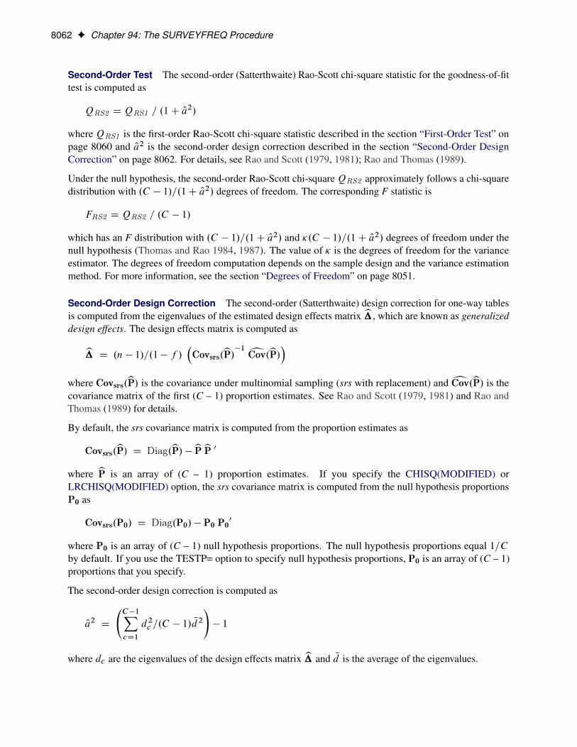
8062 F Chapter 94: The SURVEYFREQ Procedure
Second-Order Test The second-order (Satterthwaite) Rao-Scott chi-square statistic for the goodness-of-fittest is computed as
QRS2 D QRS1 = .1C Oa2/
where QRS1 is the first-order Rao-Scott chi-square statistic described in the section “First-Order Test” onpage 8060 and Oa2 is the second-order design correction described in the section “Second-Order DesignCorrection” on page 8062. For details, see Rao and Scott (1979, 1981); Rao and Thomas (1989).
Under the null hypothesis, the second-order Rao-Scott chi-square QRS2 approximately follows a chi-squaredistribution with .C � 1/=.1C Oa2/ degrees of freedom. The corresponding F statistic is
FRS2 D QRS2 = .C � 1/
which has an F distribution with .C � 1/=.1C Oa2/ and �.C � 1/=.1C Oa2/ degrees of freedom under thenull hypothesis (Thomas and Rao 1984, 1987). The value of � is the degrees of freedom for the varianceestimator. The degrees of freedom computation depends on the sample design and the variance estimationmethod. For more information, see the section “Degrees of Freedom” on page 8051.
Second-Order Design Correction The second-order (Satterthwaite) design correction for one-way tablesis computed from the eigenvalues of the estimated design effects matrix b�, which are known as generalizeddesign effects. The design effects matrix is computed as
b� D .n � 1/=.1 � f /�Covsrs.bP/�1 bCov.bP/�
where Covsrs.bP/ is the covariance under multinomial sampling (srs with replacement) and bCov.bP/ is thecovariance matrix of the first (C – 1) proportion estimates. See Rao and Scott (1979, 1981) and Rao andThomas (1989) for details.
By default, the srs covariance matrix is computed from the proportion estimates as
Covsrs.bP/ D Diag.bP/ �bPbP 0where bP is an array of (C – 1) proportion estimates. If you specify the CHISQ(MODIFIED) orLRCHISQ(MODIFIED) option, the srs covariance matrix is computed from the null hypothesis proportionsP0 as
Covsrs.P0/ D Diag.P0/ � P0 P00
where P0 is an array of (C – 1) null hypothesis proportions. The null hypothesis proportions equal 1=Cby default. If you use the TESTP= option to specify null hypothesis proportions, P0 is an array of (C – 1)proportions that you specify.
The second-order design correction is computed as
Oa2 D
C�1XcD1
d2c =.C � 1/Nd2
!� 1
where dc are the eigenvalues of the design effects matrix b� and Nd is the average of the eigenvalues.

Statistical Computations F 8063
Two-Way TablesFor two-way tables, the CHISQ option provides a Rao-Scott (design-based) test of association betweenthe row and column variables. PROC SURVEYFREQ provides a first-order Rao-Scott chi-square test bydefault. If you specify the CHISQ(SECONDORDER) option, PROC SURVEYFREQ provides a second-order(Satterthwaite) Rao-Scott chi-square test.
First-Order Test The first-order Rao-Scott chi-square statistic is computed as
QRS1 D QP = D
where QP is the Pearson chi-square based on the estimated totals and D is the design correction described inthe section “First-Order Design Correction” on page 8063. See Rao and Scott (1979, 1984, 1987) for details.
For a two-way tables with R rows and C columns, the Pearson chi-square is computed as
QP D .n=bN/ Xr
Xc
.bN rc �Erc/2 = Erc
where n is the sample size, bN is the estimated overall total, bN rc is the estimated total for table cell (r, c), andErc is the expected total for table cell (r,c) under the null hypothesis of no association,
Erc D bN r �bN �c = bN
Under the null hypothesis of no association, the first-order Rao-Scott chi-squareQRS1 approximately followsa chi-square distribution with (R – 1)(C – 1) degrees of freedom. A better approximation can be obtained bythe F statistic,
F1 D QRS1 = .R � 1/.C � 1/
which has an F distribution with .R � 1/.C � 1/ and �.R � 1/.C � 1/ degrees of freedom under the nullhypothesis (Thomas and Rao 1984, 1987). The value of � is the degrees of freedom for the variance estimator.The degrees of freedom computation depends on the sample design and the variance estimation method. Formore information, see the section “Degrees of Freedom” on page 8051.
First-Order Design Correction By default for a first-order test, PROC SURVEYFREQ computes the de-sign correction from proportion estimates. If you specify the CHISQ(MODIFIED) or LRCHISQ(MODIFIED)option for a first-order test, the procedure computes the design correction from null hypothesis proportions.
Second-order tests, which you request by specifying the CHISQ(SECONDORDER) orLRCHISQ(SECONDORDER) option, are computed by applying both first-order and second-order de-sign corrections to the weighted chi-square statistic. For second-order tests for two-way tables, PROCSURVEYFREQ always uses null hypothesis proportions to compute both the first-order and second-orderdesign corrections.
The first-order design correction D that is based on proportion estimates is computed as
D D� P
r
Pc.1 �
bP rc/ Deff.bP rc/ �Pr.1 �bP r �/ Deff.bP r �/
�Pc.1 �
bP �c/ Deff.bP �c/� = .R � 1/.C � 1/

8064 F Chapter 94: The SURVEYFREQ Procedure
where
Deff.bP rc/ D bVar.bP rc/ = Varsrs.bP rc/D Var.bP rc/ = �.1 � f / bP rc .1 � bP rc/ = .n � 1/�
as described in the section “Design Effect” on page 8052. bP rc is the estimate of the proportion in tablecell (r, c), bVar.bP rc/ is the variance of the estimate, f is the overall sampling fraction, and n is the numberof observations in the sample. The factor (1 – f ) is included only for Taylor series variance estimation(VARMETHOD=TAYLOR) when you specify the RATE= or TOTAL= option. See the section “DesignEffect” on page 8052 for details.
The design effects for the estimate of the proportion in row r and the estimate of the proportion in column c(Deff.bP r �/ and Deff.bP �c/, respectively) are computed in the same way.
If you specify the CHISQ(MODIFIED) or LRCHISQ(MODIFIED) option for a first-order Rao-Scott test, or if you request a second-order test for a two-way table (CHISQ(SECONDORDER) orLRCHISQ(SECONDORDER)), the procedure computes the design correction from the null hypothesis cellproportions instead of the estimated cell proportions. For two-way tables, the null hypothesis cell proportionsare computed as the products of the corresponding row and column proportion estimates. The modifieddesign correction D0 (based on null hypothesis proportions) is computed as
D0 D� P
r
Pc.1 � P
0rc/ Deff0.bP rc/ �Pr.1 �
bP r �/ Deff.bP r �/�Pc.1 �
bP �c/ Deff.bP �c/� = .R � 1/.C � 1/where
P 0rc D
bP r � � bP �cand
Deff0.bP rc/ D bVar.bP rc/ = Varsrs.P 0rc/
D bVar.bP rc/ = �.1 � f / P 0rc .1 � P
0rc/ = .n � 1/
�Second-Order Test The second-order (Satterthwaite) Rao-Scott chi-square statistic for two-way tables iscomputed as
QRS2 D QRS1 = .1C Oa2/
where QRS1 is the first-order Rao-Scott chi-square statistic described in the section “First-Order Test” onpage 8063 and Oa2 is the second-order design correction described in the section “Second-Order DesignCorrection” on page 8065. See Rao and Scott (1979, 1981) and Rao and Thomas (1989) for details.
Under the null hypothesis, the second-order Rao-Scott chi-square QRS2 approximately follows a chi-squaredistribution with .R � 1/.C � 1/=.1C Oa2/ degrees of freedom. The corresponding F statistic is
FRS2 D QRS2 .1C Oa2/ = .R � 1/.C � 1/
which has an F distribution with .R�1/.C �1/=.1C Oa2/ and �.R�1/.C �1/=.1C Oa2/ degrees of freedomunder the null hypothesis (Thomas and Rao 1984, 1987). The value of � is the degrees of freedom for thevariance estimator. The degrees of freedom computation depends on the sample design and the varianceestimation method. For more information, see the section “Degrees of Freedom” on page 8051.

Statistical Computations F 8065
Second-Order Design Correction The second-order (Satterthwaite) design correction for two-way tablesis computed from the eigenvalues of the estimated design effects matrix b�, which are known as generalizeddesign effects. The design effects matrix is defined as
b� D .n � 1/=.1 � f /�Covsrs.bP/�1 H bCov.bP/ H 0
�where bCov.bP/ is the covariance matrix of the R � C proportion estimates and Covsrs.bP/ is the covarianceunder multinomial sampling (srs with replacement). See Rao and Scott (1979, 1981) and Rao and Thomas(1989) for details.
The second-order design correction is computed from the design effects matrix b� as
Oa2 D
KXiD1
d2c =KNd2
!� 1
where K = (R – 1)(C – 1), dc are the eigenvalues of b�, and Nd is the average eigenvalue.
The srs covariance matrix is computed as
Covsrs.bP/ D bPr ˝bPc
wherebPr is an .R�1/� .R�1/ matrix that is constructed from the array of (R – 1) row proportion estimatesbpr as
bPr D Diag.bpr/ �bprbp 0rSimilarly,bPc is a .C � 1/ � .C � 1/ matrix that is constructed from the array of (C – 1) column proportionestimatesbpc as
bPc D Diag.bpc/ �bpcbp 0cThe .R � 1/.C � 1/ � .R � 1/.C � 1/ matrix H is computed as
H D Jr ˝ Jc � .bpr l 0r /˝ Jc � Jr ˝ .bpr l 0r /
where Jr D .I.R�1/j0/, Jc D .I.C�1/j0/, lr is an .R � 1/ array of ones, and lc is an .C � 1/ array of ones.See Rao and Scott (1979, p. 61) for details.
Rao-Scott Likelihood Ratio Chi-Square Test
The Rao-Scott likelihood ratio chi-square test is a design-adjusted version of the likelihood ratio test, whichinvolves ratios of observed and expected frequencies. For details about design-adjusted chi-square tests, seeLohr (2010, Section 10.3.2), Rao and Scott (1981, 1984, 1987); Thomas, Singh, and Roberts (1996).
PROC SURVEYFREQ provides a first-order Rao-Scott likelihood ratio test by default. If you specifythe LRCHISQ(SECONDORDER) option, PROC SURVEYFREQ provides a second-order (Satterthwaite)likelihood ratio chi-square test.
The procedure computes the Rao-Scott likelihood ratio test by applying design adjustments to the weightedlikelihood ratio statistic that is based on estimated totals. This computation is identical to the Rao-Scottchi-square test computation except that it uses the likelihood ratio statistic G2 in place of the Pearsonchi-square statistic QP . See the section “Rao-Scott Chi-Square Test” on page 8060 for details.

8066 F Chapter 94: The SURVEYFREQ Procedure
One-Way TablesFor one-way tables, the LRCHISQ option provides a Rao-Scott (design-based) goodness-of-fit test forone-way tables. By default, this is a test for the null hypothesis of equal proportions. If you specify nullhypothesis proportions in the TESTP= option, the goodness-of-fit test uses the specified proportions.
The Rao-Scott likelihood ratio test uses the likelihood ratio statistic that is based on the estimated totals,
G2 D 2 . n = bN /Xc
bN c ln�bN c = Ec
�where n is the sample size, bN is the estimated overall total, bN c is the estimated total for level c, and Ec is theexpected total for level c under the null hypothesis. For the null hypothesis of equal proportions, the expectedtotal for each level equals
Ec D bN = C
For specified null proportions, the expected total for level c equals
Ec D bN � P 0c
where P 0c is the null proportion that you specify for level c.
The computation of the Rao-Scott likelihood ratio test for one-way tables uses G2 in place of QP in theRao-Scott chi-square test computation and is otherwise identical to the chi-square test computation. See thesections “First-Order Test” on page 8060 and “Second-Order Test” on page 8062 for details.
If you specify the LRCHISQ(MODIFIED) option, PROC SURVEYFREQ computes the design correctionsby using null hypothesis proportions instead of proportion estimates. By default, null hypothesis proportionsare equal proportions for all levels of the one-way table. Alternatively, you can specify null proportion valuesin the TESTP= option.
Two-Way TablesFor two-way tables, the LRCHISQ option provides a Rao-Scott (design-based) test of association betweenthe row and column variables.
The Rao-Scott likelihood ratio test uses the likelihood ratio statistic that is based on the estimated totals,
G2 D 2 .n=bN/ Xr
Xc
bN rc ln�bN rc = Erc
�where n is the sample size, bN is the estimated overall total, bN rc is the estimated total for table cell (r, c), andErc is the expected total for cell (r, c) under the null hypothesis of no association. The expected total for cell(r, c) equals
Erc D bN r �bN �c = bN
The computation of the Rao-Scott likelihood ratio test for two-way tables uses G2 in place of QP in theRao-Scott chi-square test computation and is otherwise identical to the chi-square test computation. See thesections “First-Order Test” on page 8063 and “Second-Order Test” on page 8064 for details.
By default for a first-order test, PROC SURVEYFREQ computes the design correction from proportionestimates. If you specify the LRCHISQ(MODIFIED) option for a first-order test, the procedure computes thedesign correction from null hypothesis proportions.
Statistical Computations F 8067
Second-order tests, which you request by specifying the LRCHISQ(SECONDORDER) option, are computedby applying both first-order and second-order design corrections to the weighted likelihood ratio statistic. Forsecond-order tests for two-way tables, PROC SURVEYFREQ always uses null hypothesis proportions tocompute both the first-order and second-order design corrections.
Wald Chi-Square Test
PROC SURVEYFREQ provides two Wald chi-square tests for independence of the row and column variablesin a two-way table: a Wald chi-square test based on the difference between observed and expected weightedcell frequencies, and a Wald log-linear chi-square test based on the log odds ratios. These statistics test forindependence of the row and column variables in two-way tables, taking into account the complex surveydesign. For information about Wald statistics and their applications to categorical data analysis, see Bedrick(1983); Koch, Freeman, and Freeman (1975); Wald (1943).
For these two tests, PROC SURVEYFREQ computes the generalized Wald chi-square statistic, the corre-sponding Wald F statistic, and also an adjusted Wald F statistic for tables larger than 2 � 2. Under the nullhypothesis of independence, the Wald chi-square statistic approximately follows a chi-square distributionwith (R – 1)(C – 1) degrees of freedom for large samples. However, it has been shown that this test canperform poorly in terms of actual significance level and power, especially for tables with a large number ofcells or for samples with a relatively small number of clusters. See Thomas and Rao (1984, 1985) and Lohr(2010) for more information. See Felligi (1980) and Hidiroglou, Fuller, and Hickman (1980) for informationabout the adjusted Wald F statistic. Thomas and Rao (1984) found that the adjusted Wald F statistic providesa more stable test than the chi-square statistic, although its power can be low when the number of sampleclusters is not large. See also Korn and Graubard (1990) and Thomas, Singh, and Roberts (1996).
If you specify the WCHISQ option in the TABLES statement, PROC SURVEYFREQ computes a Waldtest for independence in the two-way table based on the differences between the observed (weighted) cellfrequencies and the expected frequencies.
Under the null hypothesis of independence of the row and column variables, the expected cell frequencies arecomputed as
Erc D bN r �bN �c = bN
where bN r � is the estimated total for row r, bN �c is the estimated total for column c, and bN is the estimatedoverall total, as described in the section “Expected Weighted Frequency” on page 8053. The null hypothesisthat the population weighted frequencies equal the expected frequencies can be expressed as
H0WYrc D Nrc � Erc D 0
for all r D 1; : : : .R � 1/ and c D 1; : : : .C � 1/. This null hypothesis can be stated equivalently in termsof cell proportions, with the expected cell proportions computed as the products of the marginal row andcolumn proportions.
The generalized Wald chi-square statistic QW is computed as
QW D bY0 .H bV.bN/ H0/�1 bYwhere bY is an array of (R – 1)(C – 1) differences between the observed and expected weighted frequencies.bN rc �Erc/, and .H bV.bN/ H0/ estimates the variance of bY.bV.bN/ is the covariance matrix of the estimates bN rc , and its computation is described in the section “Covari-ance of Totals” on page 8040.

8068 F Chapter 94: The SURVEYFREQ Procedure
H is an (R – 1)(C – 1) by RC matrix that contains the partial derivatives of the elements of bY with respect tothe elements of bN. The elements of H are computed as follows, where a denotes a row different from row r,and b denotes a column different from column c:
@bY rc=@bN rc D 1 ��bN r � C bN �c � bN �c bN r � = bN� = bN
@bY rc=@bN ac D �
�bN r � � bN r �bN �c = bN� = bN
@bY rc=@bN rb D �
�bN �c � bN r �bN �c = bN� = bN
@bY rc=@bY ab D bN r �bN �c = bN 2
Under the null hypothesis of independence, the statistic QW approximately follows a chi-square distributionwith (R – 1)(C – 1) degrees of freedom for large samples.
PROC SURVEYFREQ computes the Wald F statistic as
FW D QW = .R � 1/.C � 1/
Under the null hypothesis of independence, FW approximately follows an F distribution with (R – 1)(C– 1) numerator degrees of freedom. The denominator degrees of freedom are the degrees of freedom forthe variance estimator and depend on the sample design and the variance estimation method. For moreinformation, see the section “Degrees of Freedom” on page 8051. Alternatively, you can use the DF= optionin the TABLES statement to specify the denominator degrees of freedom.
For tables larger than 2 � 2, PROC SURVEYFREQ also computes the adjusted Wald F statistic as
FAdj_W D QW .s � k C 1/ = .ks/
where k = (R – 1)(C – 1), and s is the degrees of freedom. (For more information, see the section “Degrees ofFreedom” on page 8051.) Alternatively, you can use the DF= option in the TABLES statement to specify thevalue of s. For 2 � 2 tables, k = (R – 1 )(C – 1) = 1, and therefore the adjusted Wald F statistic equals the(unadjusted) Wald F statistic and has the same numerator and denominator degrees of freedom.
Under the null hypothesis, FAdj_W approximately follows an F distribution with k numerator degrees offreedom and (s – k + 1) denominator degrees of freedom.
Wald Log-Linear Chi-Square Test
If you specify the WLLCHISQ option in the TABLES statement, PROC SURVEYFREQ computes a Waldtest for independence based on the log odds ratios. See the section “Wald Chi-Square Test” on page 8067 formore information about Wald tests.
For a two-way table of R rows and C columns, the Wald log-linear test is based on the (R – 1)(C – 1)-dimensional array of elements bY rc ,bY rc D log bN rc � log bN rC � log bNRc C log bNRC
where bN rc is the estimated total for table cell (r, c). The null hypothesis of independence between the rowand column variables can be expressed as H0WYrc D 0 for all r D 1; : : : .R � 1/ and c D 1; : : : .C � 1/.This null hypothesis can be stated equivalently in terms of cell proportions.

Output Data Sets F 8069
The generalized Wald log-linear chi-square statistic is computed as
QL D bY0 bV.bY/�1 bYwhere bY is the (R – 1)(C – 1)-dimensional array of the bY rc , and bV.bY/ estimates the variance of bY,
bV.bY/ D A D�1 bV .bN/ D�1 A0
where bV.bN/ is the covariance matrix of the estimates bN rc , which is computed as described in the section“Covariance of Totals” on page 8040. D is a diagonal matrix with the estimated totals bN rc on the diagonal,and A is the .R � 1/.C � 1/ by RC �RC linear contrast matrix.
Under the null hypothesis of independence, the statistic QL approximately follows a chi-square distributionwith (R – 1)(C – 1) degrees of freedom for large samples.
PROC SURVEYFREQ computes the Wald log-linear F statistic as
FL D QL = .R � 1/.C � 1/
Under the null hypothesis of independence, FL approximately follows an F distribution with (R – 1)(C – 1)numerator degrees of freedom. PROC SURVEYFREQ computes the denominator degrees of freedom asdescribed in the section “Degrees of Freedom” on page 8051. Alternatively, you can use the DF= option inthe TABLES statement to specify the denominator degrees of freedom.
For tables larger than 2 � 2, PROC SURVEYFREQ also computes the adjusted Wald log-linear F statistic as
FAdj_L D QL .s � k C 1/ = .ks/
where k = (R – 1)(C – 1), and s is the denominator degrees of freedom, which is computed as described inthe section “Degrees of Freedom” on page 8051. Alternatively, you can use the DF= option in the TABLESstatement to specify the value of s. For 2� 2 tables, k = (R – 1)(C – 1) = 1, and therefore the adjusted Wald Fstatistic equals the (unadjusted) Wald F statistic and has the same numerator and denominator degrees offreedom.
Under the null hypothesis, FAdj_L approximately follows an F distribution with k numerator degrees offreedom and (s – k + 1) denominator degrees of freedom.
Output Data SetsYou can use the Output Delivery System to create a SAS data set from any piece of PROC SURVEYFREQoutput. See the section “ODS Table Names” on page 8077 and Example 94.3 for more information.
PROC SURVEYFREQ also provides an output data set that stores the replicate weights for BRR or jackknifevariance estimation and an output data set that stores the jackknife coefficients for jackknife varianceestimation.
Replicate Weight Output Data Set
If you specify the OUTWEIGHTS= method-option for VARMETHOD=BRR or VARMETHOD=JACKKNIFE,PROC SURVEYFREQ stores the replicate weights in an output data set. The OUTWEIGHTS= outputdata set contains all observations from the DATA= input data set that are valid (used in the analysis). A

8070 F Chapter 94: The SURVEYFREQ Procedure
valid observation must have a positive value of the WEIGHT variable. A valid observations must also havenonmissing values of the STRATA and CLUSTER variables unless you specify the MISSING option in thePROC SURVEYFREQ statement. See the section “Data Summary Table” on page 8070 for details aboutvalid observations.
The OUTWEIGHTS= data set contains the following variables:
• all variables in the DATA= input data set
• RepWt_1, RepWt_2, : : :, RepWt_n, which are the replicate weight variables, where n is the totalnumber of replicates in the analysis
Each replicate weight variable contains the replicate weights for the corresponding replicate. Replicateweights equal zero for those observations not included in the replicate.
After the procedure creates and stores replicate weights for a particular input data set and survey design, youcan use them again in subsequent analyses, either in PROC SURVEYFREQ or in another survey procedure.You use a REPWEIGHTS statement to provide replicate weights to the procedure.
Jackknife Coefficient Output Data Set
If you specify the OUTJKCOEFS= method-option for VARMETHOD=JACKKNIFE, PROC SURVEYFREQstores the jackknife coefficients in an output data set. The OUTJKCOEFS= output data set contains oneobservation for each replicate. The OUTJKCOEFS= data set contains the following variables:
• Replicate, which is the replicate number for the jackknife coefficient
• JKCoefficient, which is the jackknife coefficient
• DonorStratum, which is the stratum of the PSU that was deleted to construct the replicate, if youspecify a STRATA statement
After the procedure creates jackknife coefficients for a particular input data set and survey design, you canuse the OUTJKCOEFS= method-option to store these coefficients and then use them again in subsequentanalyses, either in PROC SURVEYFREQ or in another survey procedure. You use the JKCOEFS= option inthe REPWEIGHTS statement to provide jackknife coefficients for the procedure.
Displayed Output
Data Summary Table
The “Data Summary” table provides information about the input data set and the sample design. PROC SUR-VEYFREQ displays this table unless you specify the NOSUMMARY option in the PROC SURVEYFREQstatement.
The “Data Summary” table displays the total number of valid observations. To be considered valid, anobservation must have a nonmissing, positive sampling weight value if you specify a WEIGHT statement.If you do not specify the MISSING option, a valid observation must also have nonmissing values forall STRATA and CLUSTER variables. The number of valid observations can differ from the number of

Displayed Output F 8071
nonmissing observations for an individual table request, which the procedure displays in the frequency orcrosstabulation tables. See the section “Missing Values” on page 8033 for more information.
PROC SURVEYFREQ displays the following information in the “Data Summary” table:
• Number of Strata, if you specify a STRATA statement
• Number of Clusters, if you specify a CLUSTER statement
• Number of Observations, which is the total number of valid observations
• Sum of Weights, which is the sum over all valid observations, if you specify a WEIGHT or REP-WEIGHTS statement
Stratum Information Table
If you specify the LIST option in the STRATA statement, PROC SURVEYFREQ displays a “StratumInformation” table. This table provides the following information for each stratum:
• Stratum Index, which is a sequential stratum identification number
• STRATA variables, which list the levels of STRATA variables for the stratum
• Number of Observations, which is the number of valid observations in the stratum
• Population Total for the stratum, if you specify the TOTAL= option
• Sampling Rate for the stratum, if you specify the TOTAL= or RATE= option. If you specify theTOTAL= option, the sampling rate is based on the number of valid observations in the stratum.
• Number of Clusters, which is the number of clusters in the stratum, if you specify a CLUSTERstatement
Variance Estimation Table
If you specify the VARMETHOD=BRR, VARMETHOD=JACKKNIFE, or NOMCAR option in the PROCSURVEYFREQ statement, the procedure displays a “Variance Estimation” table. If you do not specify anyof these options, the procedure creates a “Variance Estimation” table but does not display it. You can storethis nondisplayed table in an output data set by using the Output Delivery System (ODS). See the section“ODS Table Names” on page 8077 for more information.
The “Variance Estimation” table provides the following information:
• Method, which is the variance estimation method—Taylor Series, Balanced Repeated Replication, orJackknife
• Replicate Weights input data set name, if you use a REPWEIGHTS statement to provide replicateweights
• Number of Replicates, if you specify VARMETHOD=BRR or VARMETHOD=JACKKNIFE

8072 F Chapter 94: The SURVEYFREQ Procedure
• Hadamard Data Set name, if you specify the HADAMARD= method-option for VARMETHOD=BRR
• Fay Coefficient, if you specify the FAY method-option for VARMETHOD=BRR
• Missing Levels Included (MISSING), if you specify the MISSING option
• Missing Levels Included (NOMCAR), if you specify the NOMCAR option
Hadamard Matrix
If you specify the PRINTH method-option for VARMETHOD=BRR, PROC SURVEYFREQ displays theHadamard matrix that it uses to construct replicates for BRR variance estimation. If you provide a Hadamardmatrix by specifying the HADAMARD= method-option for VARMETHOD=BRR but the procedure doesnot use the entire matrix, the procedure displays only the rows and columns that are actually used to constructreplicates.
One-Way Frequency Tables
PROC SURVEYFREQ displays one-way frequency tables for all one-way table requests in the TABLESstatements, unless you specify the NOPRINT option in the TABLES statement. A one-way table shows thesample frequency distribution of a single variable, and provides estimates for its population distribution interms of totals and proportions.
If you request a one-way table without specifying options, PROC SURVEYFREQ displays the followinginformation for each level of the variable:
• Frequency count, which is the number of sample observations in the level
• Weighted Frequency, which estimates the population total for the level
• Standard Deviation of Weighted Frequency
• Percent, which estimates the population proportion for the level
• Standard Error of Percent
The one-way table displays weighted frequencies if your analysis includes a WEIGHT or REPWEIGHTSstatement, or if you specify the WTFREQ option in the TABLES statement.
The one-way table also displays the Frequency Missing, which is the number of observations with missingvalues.
You can suppress the frequency counts by specifying the NOFREQ option in the TABLES statement. Also,the NOWT option suppresses the weighted frequencies and their standard deviations. The NOPERCENToption suppresses the percentages and their standard errors. The NOSTD option suppresses the standarderrors of the percentages and the standard deviations of the weighted frequencies. The NOTOTAL optionsuppresses the total row of the one-way table.
PROC SURVEYFREQ optionally displays the following information in a one-way table:
• Variance of Weighted Frequency, if you specify the VARWT option
• Confidence Limits for Weighted Frequency, if you specify the CLWT option
Displayed Output F 8073
• Coefficient of Variation for Weighted Frequency, if you specify the CVWT option
• Test Percent, if you specify the TESTP= option
• Variance of Percent, if you specify the VAR option
• Confidence Limits for Percent, if you specify the CL option
• Coefficient of Variation for Percent, if you specify the CV option
• Design Effect for Percent, if you specify the DEFF option
Crosstabulation Tables
PROC SURVEYFREQ displays all table requests in the TABLES statements, unless you specify theNOPRINT option in the TABLES statement. For two-way to multiway crosstabulation tables, the values ofthe last variable in the table request form the table columns. The values of the next-to-last variable form therows. Each level (or combination of levels) of the other variables forms one layer. PROC SURVEYFREQproduces a separate two-way crosstabulation table for each layer of a multiway table.
For each layer, the crosstabulation table displays the row and column variable names and values (levels).Each two-way table lists levels of the column variable within each level of the row variable.
By default, the procedure displays all levels of the column variable within each level of the row variables,including any column variable levels with zero frequency for that row. For multiway tables, the proceduredisplays all levels of the row variable for each layer of the table by default, including any row levels with zerofrequency for that layer. You can suppress the display of zero frequency levels by specifying the NOSPARSEoption.
If you request a crosstabulation table without specifying options, the table displays the following informationfor each combination of variable levels (table cell):
• Frequency, which is the number of sample observations in the table cell
• Weighted Frequency, which estimates the population total for the table cell
• Standard Deviation of Weighted Frequency
• Percent, which estimates the population proportion for the table cell
• Standard Error of Percent
The two-way table displays weighted frequencies if your analysis includes a WEIGHT or REPWEIGHTSstatement, or if you specify the WTFREQ option in the TABLES statement.
The two-way table also displays the Frequency Missing, which is the number of observations with missingvalues.
You can suppress the frequency counts by specifying the NOFREQ option in the TABLES statement. Also,the NOWT option suppresses the weighted frequencies and their standard deviations. The NOPERCENToption suppresses all percentages and their standard errors. The NOCELLPERCENT option suppressesoverall cell percentages and their standard errors, but displays any other percentages (and standard errors)that you request, such as row or column percentages. The NOSTD option suppresses the standard errors of

8074 F Chapter 94: The SURVEYFREQ Procedure
the percentages and the standard deviations of the weighted frequencies. The NOTOTAL option suppressesthe row totals and column totals, as well as the overall total.
PROC SURVEYFREQ optionally displays the following information in a two-way table:
• Expected Weighted Frequency, if you specify the EXPECTED option
• Deviation from Expected Weighted Frequency, if you specify the DEVIATION option
• Pearson Residual, if you specify the PEARSONRES option
• Cell Chi-Square, if you specify the CELLCHI2 option
• Variance of Weighted Frequency, if you specify the VARWT option
• Confidence Limits for Weighted Frequency, if you specify the CLWT option
• Coefficient of Variation for Weighted Frequency, if you specify the CVWT option
• Variance of Percent, if you specify the VAR option
• Confidence Limits for Percent, if you specify the CL option
• Coefficient of Variation for Percent, if you specify the CV option
• Design Effect for Percent, if you specify the DEFF option
• Row Percent, which estimates the population proportion of the row total, if you specify the ROWoption
• Standard Error of Row Percent, if you specify the ROW option
• Variance of Row Percent, if you specify the VAR option and the ROW option
• Confidence Limits for Row Percent, if you specify the CL option and the ROW option
• Coefficient of Variation for Row Percent, if you specify the CV option and the ROW option
• Design Effect for Row Percent, if you specify the ROW(DEFF) option
• Column Percent, which estimates the population proportion of the column total, if you specify theCOLUMN option
• Standard Error of Column Percent, if you specify the COLUMN option
• Variance of Column Percent, if you specify the VAR option and the COLUMN option
• Confidence Limits for Column Percent, if you specify the CL option and the COLUMN option
• Coefficient of Variation for Column Percent, if you specify the CV option and the COLUMN option
• Design Effects for Column Percent, if you specify the COLUMN(DEFF) option

Displayed Output F 8075
Statistical Tests
If you specify the CHISQ option for the Rao-Scott chi-square test or the LRCHISQ option for the Rao-Scottlikelihood ratio chi-square test, PROC SURVEYFREQ displays the following information:
• Pearson Chi-Square, if you specify the CHISQ option
• Likelihood Ratio Chi-Square, if you specify the LRCHISQ option
• Design Correction
• Rao-Scott Chi-Square, by default or if you specify the FIRSTORDER option
• First-Order Chi-Square, if you specify the SECONDORDER option
• Second-Order Chi-Square, if you specify the SECONDORDER option
• DF, which is the degrees of freedom for the chi-square test
• Pr > ChiSq, which is the p-value for the chi-square test
• F Value
• Num DF, which is the numerator degrees of freedom for F
• Den DF, which is the denominator degrees of freedom for F
• Pr > F, which is the p-value for the F test
If you specify the WCHISQ option for the Wald chi-square test or the WLLCHISQ option for the Waldlog-linear chi-square test, PROC SURVEYFREQ displays the following information:
• Wald Chi-Square, if you specify the WCHISQ option
• Wald Log-Linear Chi-Square, if you specify the WLLCHISQ option
• F Value
• Num DF, which is the numerator degrees of freedom for F
• Den DF, which is the denominator degrees of freedom for F
• Pr > F, which is the p-value for the F test
• Adjusted F Value, for tables larger than 2 � 2
• Num DF, which is the numerator degrees of freedom for Adjusted F
• Den DF, which is the denominator degrees of freedom for Adjusted F
• Pr > Adj F, which is the p-value for the Adjusted F test

8076 F Chapter 94: The SURVEYFREQ Procedure
Risks and Risk Difference
If you specify the RISK option in the TABLES statement for a 2 � 2 table, PROC SURVEYFREQ displays“Column 1 Risk Estimates” and “Column 2 Risk Estimates” tables. You can display only column 1 or column2 risks by specifying the RISK1 or RISK2 option, respectively.
The “Risk Estimates” table displays the following information for Row 1, Row 2, Total, and Difference:
• Row, which identifies the risk as Row 1, Row 2, Total, or Difference
• Risk estimate
• Standard Error
• Confidence Limits
In the “Column 1 Risk Estimates” table, the row 1 risk is the column 1 percentage of row 1. The row 2 risk isthe column 1 percentage of row 2, and the total risk is the column 1 percentage of the entire table. The riskdifference is the row 1 risk minus the row 2 risk. In the “Column 2 Risk Estimates” table, these computationsare based on column 2.
Odds Ratio and Relative Risks
If you specify the OR option in the TABLES statement for a 2 � 2 table, PROC SURVEYFREQ displays the“Odds Ratio” table. This table includes the following information:
• Statistic, which identifies the statistic as the Odds Ratio, the Column 1 Relative Risk, or the Column 2Relative Risk
• Estimate
• Confidence Limits
Kappa Statistics
If you specify the AGREE, KAPPA, or WTKAPPA option in the TABLES statement for a square table,PROC SURVEYFREQ displays the “Kappa Statistics” table. This table includes the following information:
• Statistic, which identifies the statistic as the Simple Kappa Coefficient or the Weighted Kappa Coeffi-cient
• Estimate
• Standard Error
• Confidence Limits

ODS Table Names F 8077
Kappa Weights
If you specify the AGREE(PRINTKWTS) or WTKAPPA(PRINTKWTS) option for a square table whosedimension is greater than 2, PROC SURVEYFREQ displays the “Kappa Weights” table. This table providesthe matrix of kappa agreement weights that the procedure uses to compute the weighted kappa coefficient.The matrix contains an agreement weight for each pair of column variable levels.
ODS Table NamesPROC SURVEYFREQ assigns a name to each table that it creates. You can use these names to refer totables when you use the Output Delivery System (ODS) to select tables and create output data sets. Formore information about ODS, see Chapter 20, “Using the Output Delivery System.” See Example 94.3 forexamples of storing PROC SURVEYFREQ tables as output data sets.
Table 94.9 lists the ODS table names together with their descriptions and the options required to produce thetables.
Table 94.9 ODS Tables Produced by PROC SURVEYFREQ
ODS Table Name Description Statement Option
ChiSq Chi-square test TABLES CHISQChiSq1 Modified chi-square test TABLES CHISQ(MODIFIED)CrossTabs Crosstabulation table TABLES n-way table request, n > 1HadamardMatrix Hadamard matrix PROC VARMETHOD=BRR(PRINTH)Kappa Kappa coefficients TABLES AGREE, KAPPA, or
WTKAPPA (r � r table)KappaWeights Kappa agreement weights TABLES WTKAPPA(PRINTKWTS)
(r � r table, r > 2)LRChiSq Likelihood ratio test TABLES LRCHISQLRChiSq1 Modified likelihood ratio test TABLES LRCHISQ(MODIFIED)OddsRatio Odds ratio and relative risks TABLES OR (2 � 2 table)OneWay One-way frequency table PROC No TABLES statement
or TABLES One-way table requestRisk1 Column 1 risk estimates TABLES RISK or RISK1 (2 � 2 table)Risk2 Column 2 risk estimates TABLES RISK or RISK2 (2 � 2 table)StrataInfo Stratum information STRATA LISTSummary Data summary PROC DefaultTableSummary Table summary (not displayed) TABLES DefaultVarianceEstimation Variance estimation PROC VARMETHOD=BRR,
VARMETHOD=JACKKNIFE,or NOMCAR
WChiSq Wald chi-square test TABLES WCHISQ (two-way table)WLLChiSq Wald log-linear chi-square test TABLES WLLCHISQ (two-way table)

8078 F Chapter 94: The SURVEYFREQ Procedure
ODS GraphicsStatistical procedures use ODS Graphics to create graphs as part of their output. ODS Graphics is describedin detail in Chapter 21, “Statistical Graphics Using ODS.”
Before you create graphs, ODS Graphics must be enabled (for example, by specifying the ODS GRAPH-ICS ON statement). For more information about enabling and disabling ODS Graphics, see the section“Enabling and Disabling ODS Graphics” on page 606 in Chapter 21, “Statistical Graphics Using ODS.”
The overall appearance of graphs is controlled by ODS styles. Styles and other aspects of using ODSGraphics are discussed in the section “A Primer on ODS Statistical Graphics” on page 605 in Chapter 21,“Statistical Graphics Using ODS.”
When ODS Graphics is enabled, you can request specific plots with the PLOTS= option in the TABLESstatement. To produce a weighted frequency plot or mosaic plot, you must specify the WTFREQPLOT orMOSAICPLOT plot-request in the PLOTS= option, or you must specify the PLOTS=ALL option. By default,PROC SURVEYFREQ produces all other plots that are associated with the analyses that you request in theTABLES statement. You can suppress default plots and request specific plots by using the PLOTS(ONLY)=option. See the description of the PLOTS= option for more information.
PROC SURVEYFREQ assigns a name to each graph that it creates with ODS Graphics. You can use thesenames to refer to the graphs. Table 94.10 lists the names of the graphs that PROC SURVEYFREQ generatestogether with their descriptions, their PLOTS= options (plot-requests), and the TABLES statement optionsthat are required to produce the graphs.
Table 94.10 ODS Graphs Produced by PROC SURVEYFREQ
ODS Graph Name Description PLOTS= Option TABLES Statement Option
KappaPlot Kappa plot KAPPAPLOT AGREE or KAPPA(h � r � r table)
MosaicPlot Mosaic plot MOSAICPLOT Two-way or multiway table requestORPlot Odds ratio plot ODDSRATIOPLOT OR (h � 2 � 2 table)RelRiskPlot Relative risk plot RELRISKPLOT OR (h � 2 � 2 table)RiskDiffPlot Risk difference plot RISKDIFFPLOT RISK (h � 2 � 2 table)WtFreqPlot Weighted frequency plot WTFREQPLOT Any table requestWtKappaPlot Weighted kappa plot WTKAPPAPLOT AGREE or WTKAPPA
(h � r � r table, r > 2)
Examples: SURVEYFREQ Procedure
Example 94.1: Two-Way TablesThis example uses the SIS_Survey data set from the section “Getting Started: SURVEYFREQ Procedure” onpage 7990. The data set contains results from a customer satisfaction survey for a student information system(SIS).

Example 94.1: Two-Way Tables F 8079
The following PROC SURVEYFREQ statements request a two-way table for Department by Response andcustomize the crosstabulation table display:
title 'Student Information System Survey';proc surveyfreq data=SIS_Survey;
tables Department * Response / cv deff nowt nostd nototal;strata State NewUser / list;cluster School;weight SamplingWeight;
run;
The TABLES statement requests a two-way table of Department by Response. The CV option requestscoefficients of variation for the percentage estimates. The DEFF option requests design effects for thepercentage estimates. The NOWT option suppresses display of the weighted frequencies, and the NOSTDoption suppresses display of standard errors for the estimates. The NOTOTAL option suppresses the rowtotals, column totals, and overall totals.
The STRATA, CLUSTER, and WEIGHT statements provide sample design information for the procedure, sothat the analysis is done according to the sample design used for the survey. The STRATA statement namesthe variables State and NewUser, which identify the first-stage strata. The LIST option in the STRATAstatement requests a “Stratum Information” table. The CLUSTER statement names the variable School,which identifies the clusters (primary sampling units). The WEIGHT statement names the sampling weightvariable.
Output 94.1.1 displays the “Data Summary” and “Stratum Information” tables produced by PROCSURVEYFREQ. The “Stratum Information” table lists the six strata in the survey and shows the num-ber of observations and the number of clusters (schools) in each stratum.
Output 94.1.1 Data Summary and Stratum Information
Student Information System Survey
The SURVEYFREQ Procedure
Data Summary
Number of Strata 6Number of Clusters 370Number of Observations 1850Sum of Weights 38899.6482
Stratum Information
Stratum Number of Number ofIndex State NewUser Obs Clusters
--------------------------------------------------------------1 GA Renewal Customer 315 632 GA New Customer 355 713 NC Renewal Customer 280 564 NC New Customer 420 845 SC Renewal Customer 210 426 SC New Customer 270 54
--------------------------------------------------------------

8080 F Chapter 94: The SURVEYFREQ Procedure
Output 94.1.2 displays the two-way table of Department by Response. According to the TABLES statementoptions that are specified, this two-way table includes coefficients of variation and design effects for thepercentage estimates, and it does not show the weighted frequencies or the standard errors of the estimates. Italso does not show the row, column, and overall totals.
Output 94.1.2 Two-Way Table of Department by Response
Table of Department by Response
CV for DesignDepartment Response Frequency Percent Percent Effect-------------------------------------------------------------------------------Faculty Very Unsatisfied 209 13.4987 0.0865 2.1586
Unsatisfied 203 13.0710 0.0868 2.0962Neutral 346 22.4127 0.0629 2.1157Satisfied 254 16.2006 0.0806 2.3232Very Satisfied 98 6.2467 0.1362 2.2842
-------------------------------------------------------------------------------Admin/Guidance Very Unsatisfied 95 3.6690 0.1277 1.1477
Unsatisfied 123 4.6854 0.1060 1.0211Neutral 235 9.1838 0.0700 0.9166Satisfied 201 7.7305 0.0756 0.8848Very Satisfied 86 3.3016 0.1252 0.9892
-------------------------------------------------------------------------------
The following PROC SURVEYFREQ statements request a two-way table of Department by Response thatincludes row percentages, and also a Wald chi-square test of association between the two table variables:
title 'Student Information System Survey';proc surveyfreq data=SIS_Survey nosummary;
tables Department * Response / row nowt wchisq;strata State NewUser;cluster School;weight SamplingWeight;
run;
Output 94.1.3 displays the two-way table. The row percentages show the distribution of Response for Depart-ment = ‘Faculty’ and for Department = ‘Admin/Guidance’. This is equivalent to a domain (subpopulation)analysis of Response, where the domains are Department = ‘Faculty’ and Department = ‘Admin/Guidance’.
Output 94.1.4 displays the Wald chi-square test of association between Department and Response. TheWald chi-square is 11.44, and the corresponding adjusted F value is 2.84 with a p-value of 0.0243. Thisindicates a significant association between department (faculty or admin/guidance) and satisfaction with thestudent information system.
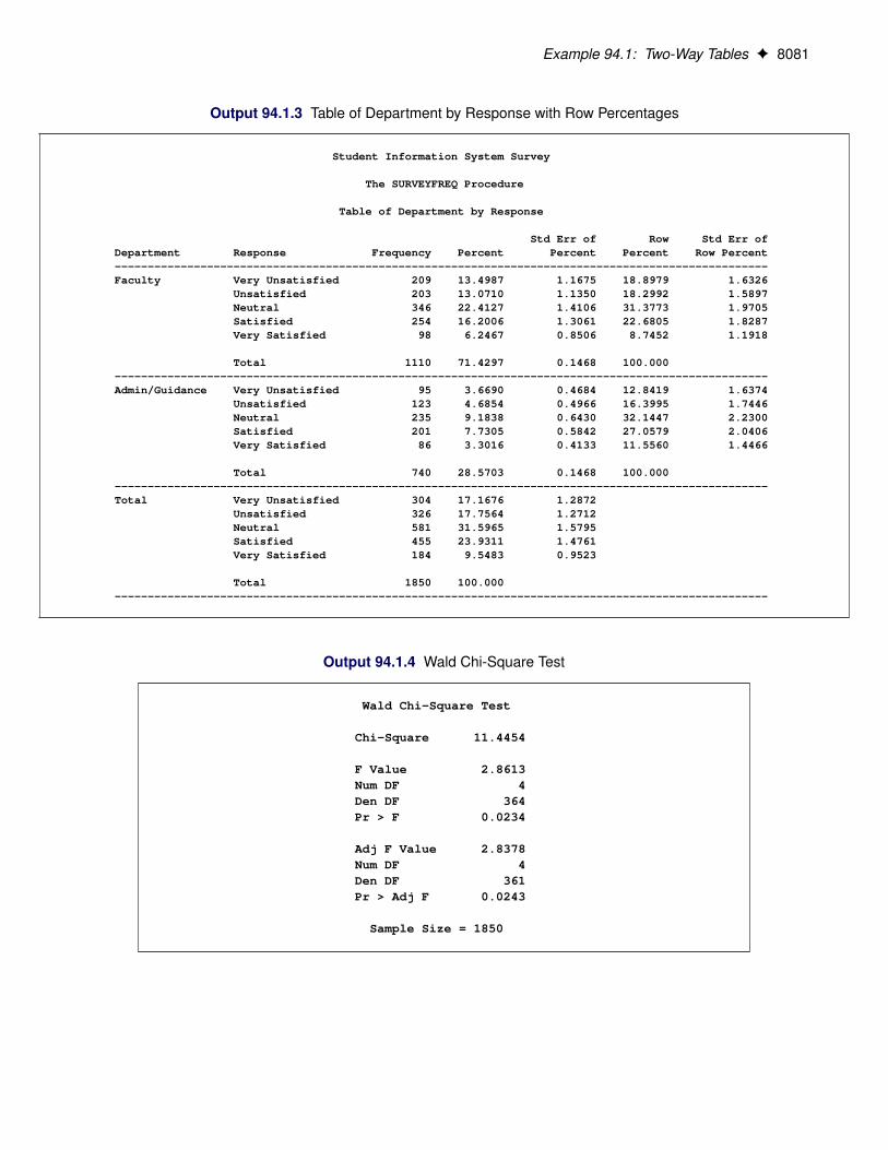
Example 94.1: Two-Way Tables F 8081
Output 94.1.3 Table of Department by Response with Row Percentages
Student Information System Survey
The SURVEYFREQ Procedure
Table of Department by Response
Std Err of Row Std Err ofDepartment Response Frequency Percent Percent Percent Row Percent---------------------------------------------------------------------------------------------------Faculty Very Unsatisfied 209 13.4987 1.1675 18.8979 1.6326
Unsatisfied 203 13.0710 1.1350 18.2992 1.5897Neutral 346 22.4127 1.4106 31.3773 1.9705Satisfied 254 16.2006 1.3061 22.6805 1.8287Very Satisfied 98 6.2467 0.8506 8.7452 1.1918
Total 1110 71.4297 0.1468 100.000---------------------------------------------------------------------------------------------------Admin/Guidance Very Unsatisfied 95 3.6690 0.4684 12.8419 1.6374
Unsatisfied 123 4.6854 0.4966 16.3995 1.7446Neutral 235 9.1838 0.6430 32.1447 2.2300Satisfied 201 7.7305 0.5842 27.0579 2.0406Very Satisfied 86 3.3016 0.4133 11.5560 1.4466
Total 740 28.5703 0.1468 100.000---------------------------------------------------------------------------------------------------Total Very Unsatisfied 304 17.1676 1.2872
Unsatisfied 326 17.7564 1.2712Neutral 581 31.5965 1.5795Satisfied 455 23.9311 1.4761Very Satisfied 184 9.5483 0.9523
Total 1850 100.000---------------------------------------------------------------------------------------------------
Output 94.1.4 Wald Chi-Square Test
Wald Chi-Square Test
Chi-Square 11.4454
F Value 2.8613Num DF 4Den DF 364Pr > F 0.0234
Adj F Value 2.8378Num DF 4Den DF 361Pr > Adj F 0.0243
Sample Size = 1850

8082 F Chapter 94: The SURVEYFREQ Procedure
Example 94.2: Multiway Tables (Domain Analysis)Continuing to use the SIS_Survey data set from the section “Getting Started: SURVEYFREQ Procedure”on page 7990, this example shows how to produce multiway tables. The following PROC SURVEYFREQstatements request a table of Department by SchoolType by Response for the student information systemsurvey:
title 'Student Information System Survey';proc surveyfreq data=SIS_Survey;
tables Department * SchoolType * ResponseSchoolType * Response;
strata State NewUser;cluster School;weight SamplingWeight;
run;
The TABLES statement requests a multiway table with SchoolType as the row variable, Response as thecolumn variable, and Department as the layer variable. This request produces a separate two-way table ofSchoolType by Response for each level of the variable Department. The TABLES statement also requests atwo-way table of SchoolType by Response, which totals the multiway table over both levels of Department.As in the previous examples, the STRATA, CLUSTER, and WEIGHT statements provide sample designinformation, so that the analysis will be done according to the design used for this survey.
Output 94.2.1 displays the multiway table produced by PROC SURVEYFREQ, which includes a tableof SchoolType by Response for Department = ‘Faculty’ and for Department = ‘Admin/Guidance’. Thisis equivalent to a domain (subpopulation) analysis of SchoolType by Response, where the domains areDepartment = ‘Faculty’ and Department = ‘Admin/Guidance’.

Example 94.2: Multiway Tables (Domain Analysis) F 8083
Output 94.2.1 Multiway Table of Department by SchoolType by Response
Student Information System Survey
The SURVEYFREQ Procedure
Table of SchoolType by ResponseControlling for Department=Faculty
Weighted Std Dev of Std Err ofSchoolType Response Frequency Frequency Wgt Freq Percent Percent----------------------------------------------------------------------------------------------------Middle School Very Unsatisfied 74 1846 301.22637 6.6443 1.0838
Unsatisfied 78 1929 283.11476 6.9428 1.0201Neutral 130 3289 407.80855 11.8369 1.4652Satisfied 113 2795 368.85087 10.0597 1.3288Very Satisfied 55 1378 261.63311 4.9578 0.9411
Total 450 11237 714.97120 40.4415 2.5713----------------------------------------------------------------------------------------------------High School Very Unsatisfied 135 3405 389.42313 12.2536 1.3987
Unsatisfied 125 3155 384.56734 11.3563 1.3809Neutral 216 5429 489.37826 19.5404 1.7564Satisfied 141 3507 417.54773 12.6208 1.5040Very Satisfied 43 1052 221.59367 3.7874 0.7984
Total 660 16549 719.61536 59.5585 2.5713----------------------------------------------------------------------------------------------------Total Very Unsatisfied 209 5251 454.82598 18.8979 1.6326
Unsatisfied 203 5085 442.39032 18.2992 1.5897Neutral 346 8718 550.81735 31.3773 1.9705Satisfied 254 6302 507.01711 22.6805 1.8287Very Satisfied 98 2430 330.97602 8.7452 1.1918
Total 1110 27786 119.25529 100.000----------------------------------------------------------------------------------------------------
Table of SchoolType by ResponseControlling for Department=Admin/Guidance
Weighted Std Dev of Std Err ofSchoolType Response Frequency Frequency Wgt Freq Percent Percent----------------------------------------------------------------------------------------------------Middle School Very Unsatisfied 42 649.43427 133.06194 5.8435 1.1947
Unsatisfied 31 460.35557 100.80158 4.1422 0.9076Neutral 104 1568 186.99946 14.1042 1.6804Satisfied 84 1269 165.71127 11.4142 1.4896Very Satisfied 39 574.93878 110.37243 5.1732 0.9942
Total 300 4521 287.86832 40.6774 2.5801----------------------------------------------------------------------------------------------------High School Very Unsatisfied 53 777.77725 136.41869 6.9983 1.2285
Unsatisfied 92 1362 175.40862 12.2573 1.5806Neutral 131 2005 212.34804 18.0404 1.8990Satisfied 117 1739 190.07798 15.6437 1.7118Very Satisfied 47 709.37033 126.54394 6.3828 1.1371
Total 440 6593 288.92483 59.3226 2.5801----------------------------------------------------------------------------------------------------Total Very Unsatisfied 95 1427 182.28132 12.8419 1.6374
Unsatisfied 123 1823 193.43045 16.3995 1.7446Neutral 235 3572 250.22739 32.1447 2.2300Satisfied 201 3007 226.82311 27.0579 2.0406Very Satisfied 86 1284 160.83434 11.5560 1.4466
Total 740 11114 60.78850 100.000----------------------------------------------------------------------------------------------------

8084 F Chapter 94: The SURVEYFREQ Procedure
Example 94.3: Output Data SetsPROC SURVEYFREQ uses the Output Delivery System (ODS) to create output data sets. This is a departurefrom older SAS procedures that provide OUTPUT statements for similar functionality. By using ODS, youcan create a SAS data set from any piece of PROC SURVEYFREQ output. For more information about ODS,see Chapter 20, “Using the Output Delivery System.”
When selecting tables for ODS output data sets, you refer to tables by their ODS table names. Each tablecreated by PROC SURVEYFREQ is assigned a name. See the section “ODS Table Names” on page 8077 fora list of the table names provided by PROC SURVEYFREQ.
To save the one-way table of Response from Figure 94.3 in an output data set, use an ODS OUTPUTstatement as follows:
proc surveyfreq data=SIS_Survey;tables Response / cl nowt;ods output OneWay=ResponseTable;strata State NewUser;cluster School;weight SamplingWeight;
run;
Output 94.3.1 displays the output data set ResponseTable, which contains the one-way table of Response.This data set has six observations, and each of these observations corresponds to a row of the one-way table.The first five observations correspond to the five levels of Response, as they are ordered in the one-way tabledisplay, and the last observation corresponds to the overall total, which is the last row of the one-way table.The data set ResponseTable includes a variable corresponding to each column of the one-way table. Forexample, the variable Percent contains the percentage estimates, and the variables LowerCL and UpperCLcontain the lower and upper confidence limits for the percentage estimates.
Output 94.3.1 ResponseTable Output Data Set
Obs Table Response Frequency Percent StdErr LowerCL UpperCL
1 Table Response Very Unsatisfied 304 17.1676 1.2872 14.6364 19.69892 Table Response Unsatisfied 326 17.7564 1.2712 15.2566 20.25623 Table Response Neutral 581 31.5965 1.5795 28.4904 34.70264 Table Response Satisfied 455 23.9311 1.4761 21.0285 26.83385 Table Response Very Satisfied 184 9.5483 0.9523 7.6756 11.42106 Table Response . 1850 100.000 _ _ _
PROC SURVEYFREQ also creates a table summary that is not displayed. Some of the information in thistable is similar to that contained in the “Data Summary” table, but the table summary describes the data thatare used to analyze the specified table, while the data summary describes the entire input data set. Due tomissing values, for example, the number of observations (or strata or clusters) used to analyze a particulartable can differ from the number of observations (or strata or clusters) reported for the input data set in the“Data Summary” table. See the section “Missing Values” on page 8033 for more details. If you requestconfidence limits, the “Table Summary” table also contains the degrees of freedom and the t-value used tocompute the confidence limits.

References F 8085
The following statements store the nondisplayed “Table Summary” table in the output data setResponseSummary:
proc surveyfreq data=SIS_Survey;tables Response / cl nowt;ods output TableSummary=ResponseSummary;strata State NewUser;cluster School;weight SamplingWeight;
run;
Output 94.3.2 displays the output data set ResponseSummary.
Output 94.3.2 ResponseSummary Output Data Set
Number Number DegreesNumber of of of of t
Obs Table Observations Strata Clusters Freedom Percentile
1 Table Response 1850 6 370 364 1.966503
References
Agresti, A. (2007), An Introduction to Categorical Data Analysis, 2nd Edition, New York: John Wiley &Sons.
Agresti, A. (2013), Categorical Data Analysis, 3rd Edition, Hoboken, NJ: John Wiley & Sons.
Agresti, A. and Coull, B. A. (1998), “Approximate Is Better Than ‘Exact’ for Interval Estimation of BinomialProportions,” American Statistician, 52, 119–126.
Bedrick, E. J. (1983), “Adjusted Chi-Squared Tests for Cross-Classified Tables of Survey Data,” Biometrika,70, 591–596.
Brick, J. M. and Kalton, G. (1996), “Handling Missing Data in Survey Research,” Statistical Methods inMedical Research, 5, 215–238.
Brown, L. D., Cai, T. T., and DasGupta, A. (2001), “Interval Estimation for a Binomial Proportion,” StatisticalScience, 16, 101–133.
Cicchetti, D. V. and Allison, T. (1971), “A New Procedure for Assessing Reliability of Scoring EEG SleepRecordings,” American Journal of EEG Technology, 11, 101–109.
Clopper, C. J. and Pearson, E. S. (1934), “The Use of Confidence or Fiducial Limits Illustrated in the Case ofthe Binomial,” Biometrika, 26, 404–413.
Cochran, W. G. (1977), Sampling Techniques, 3rd Edition, New York: John Wiley & Sons.
Cohen, J. (1960), “A Coefficient of Agreement for Nominal Scales,” Educational and Psychological Mea-surement, 20, 37–46.
8086 F Chapter 94: The SURVEYFREQ Procedure
Curtin, L. R., Kruszon-Moran, D., Carroll, M., and Li, X. (2006), “Estimation and Analytic Issues for RareEvents in NHANES,” in Proceedings of the Survey Research Methods Section, 2893–2903, Alexandria,VA: American Statistical Association.
Dippo, C. S., Fay, R. E., and Morganstein, D. H. (1984), “Computing Variances from Complex Samples withReplicate Weights,” in Proceedings of the Survey Research Methods Section, 489–494, Alexandria, VA:American Statistical Association.
Fay, R. E. (1989), “Theory and Application of Replicate Weighting for Variance Calculations,” in Proceedingsof the Survey Research Methods Section, 212–217, Alexandria, VA: American Statistical Association.
Felligi, I. P. (1980), “Approximate Tests of Independence and Goodness of Fit Based on Stratified MultistageSamples,” Journal of the American Statistical Association, 75, 261–268.
Fienberg, S. E. (1980), The Analysis of Cross-Classified Categorical Data, 2nd Edition, Cambridge, MA:MIT Press.
Fleiss, J. L. (1981), Statistical Methods for Rates and Proportions, 2nd Edition, New York: John Wiley &Sons.
Fleiss, J. L. and Cohen, J. (1973), “The Equivalence of Weighted Kappa and the Intraclass CorrelationCoefficient as Measures of Reliability,” Educational and Psychological Measurement, 33, 613–619.
Fleiss, J. L., Cohen, J., and Everitt, B. S. (1969), “Large-Sample Standard Errors of Kappa and WeightedKappa,” Psychological Bulletin, 72, 323–327.
Fleiss, J. L., Levin, B., and Paik, M. C. (2003), Statistical Methods for Rates and Proportions, 3rd Edition,Hoboken, NJ: John Wiley & Sons.
Friendly, M. (2000), Visualizing Categorical Data, Cary, NC: SAS Institute Inc.
Fuller, W. A. (1975), “Regression Analysis for Sample Survey,” Sankhy Na, Series C, 37, 117–132.
Fuller, W. A., Kennedy, W. J., Schnell, D., Sullivan, G., and Park, H. J. (1989), PC CARP, Ames: Iowa StateUniversity Statistical Laboratory.
Hansen, M. H., Hurwitz, W. N., and Madow, W. G. (1953), Sample Survey Methods and Theory, volume 1and 2, New York: John Wiley & Sons.
Hidiroglou, M. A., Fuller, W. A., and Hickman, R. D. (1980), SUPER CARP, Ames: Iowa State UniversityStatistical Laboratory.
Judkins, D. R. (1990), “Fay’s Method for Variance Estimation,” Journal of Official Statistics, 6, 223–239.
Kalton, G. (1983), Introduction to Survey Sampling, Sage University Paper Series on Quantitative Applica-tions in the Social Sciences, 07-035, Beverly Hills, CA: Sage Publications.
Kalton, G. and Kasprzyk, D. (1986), “The Treatment of Missing Survey Data,” Survey Methodology, 12,1–16.
Kish, L. (1965), Survey Sampling, New York: John Wiley & Sons.
Koch, G. G., Freeman, D. H., and Freeman, J. L. (1975), “Strategies in the Multivariate Analysis of Datafrom Complex Surveys,” International Statistical Review, 43, 59–78.

References F 8087
Koch, G. G., Landis, J. R., Freeman, J. L., Freeman, D. H., and Lehnen, R. G. (1977), “A General Methodologyfor the Analysis of Experiments with Repeated Measurement of Categorical Data,” Biometrics, 33, 133–158.
Korn, E. L. and Graubard, B. I. (1990), “Simultaneous Testing with Complex Survey Data: Use of Bonferronit-Statistics,” American Statistician, 44, 270–276.
Korn, E. L. and Graubard, B. I. (1998), “Confidence Intervals for Proportions with Small Expected Numberof Positive Counts Estimated from Survey Data,” Survey Methodology, 24, 193–201.
Korn, E. L. and Graubard, B. I. (1999), Analysis of Health Surveys, New York: John Wiley & Sons.
Lee, E. S., Forthofer, R. N., and Lorimor, R. J. (1989), Analyzing Complex Survey Data, Sage University PaperSeries on Quantitative Applications in the Social Sciences, 07-071, Beverly Hills, CA: Sage Publications.
Leemis, L. M. and Trivedi, K. S. (1996), “A Comparison of Approximate Interval Estimators for the BernoulliParameter,” American Statistician, 50, 63–68.
Levy, P. S. and Lemeshow, S. (1999), Sampling of Populations: Methods and Applications, 3rd Edition, NewYork: John Wiley & Sons.
Lohr, S. L. (2010), Sampling: Design and Analysis, 2nd Edition, Boston: Brooks/Cole.
Nathan, G. (1975), “Tests for Independence in Contingency Tables from Stratified Samples,” Sankhy Na, SeriesC, 37, 77–87.
Newcombe, R. G. (1998), “Two-Sided Confidence Intervals for the Single Proportion: Comparison of SevenMethods,” Statistics in Medicine, 17, 857–872.
Rao, J. N. K. and Scott, A. J. (1979), “Chi-Squared Tests for Analysis of Categorical Data from ComplexSurveys,” in Proceedings of the Survey Research Methods Section, 58–66, Washington, DC: AmericanStatistical Association.
Rao, J. N. K. and Scott, A. J. (1981), “The Analysis of Categorical Data from Complex Surveys: Chi-SquaredTests for Goodness of Fit and Independence in Two-Way Tables,” Journal of the American StatisticalAssociation, 76, 221–230.
Rao, J. N. K. and Scott, A. J. (1984), “On Chi-Squared Tests for Multiway Contingency Tables with CellProperties Estimated from Survey Data,” Annals of Statistics, 12, 46–60.
Rao, J. N. K. and Scott, A. J. (1987), “On Simple Adjustments to Chi-Square Tests with Survey Data,” Annalsof Statistics, 15, 385–397.
Rao, J. N. K. and Shao, J. (1996), “On Balanced Half-Sample Variance Estimation in Stratified RandomSampling,” Journal of the American Statistical Association, 91, 343–348.
Rao, J. N. K. and Shao, J. (1999), “Modified Balanced Repeated Replication for Complex Survey Data,”Biometrika, 86, 403–415.
Rao, J. N. K. and Thomas, D. R. (1989), “Chi-Squared Tests for Contingency Tables,” in C. J. Skinner,D. Holt, and T. M. F. Smith, eds., Analysis of Complex Surveys, 89–114, New York: John Wiley & Sons.
Särndal, C. E., Swensson, B., and Wretman, J. (1992), Model Assisted Survey Sampling, New York: Springer-Verlag.

8088 F Chapter 94: The SURVEYFREQ Procedure
Satterthwaite, F. E. (1946), “An Approximate Distribution of Estimates of Variance Components,” BiometricsBulletin, 2, 110–114.
Stokes, M. E., Davis, C. S., and Koch, G. G. (2000), Categorical Data Analysis Using the SAS System, 2ndEdition, Cary, NC: SAS Institute Inc.
Sukasih, A. and Jang, D. (2005), “An Application of Confidence Interval Methods for Small Proportions inthe Health Care Survey of DoD Beneficiaries,” in Proceedings of the Survey Research Methods Section,3608–3612, Alexandria, VA: American Statistical Association.
Thomas, D. R. and Rao, J. N. K. (1984), “A Monte Carlo Study of Exact Levels of Goodness-of-Fit Statisticsunder Cluster Sampling,” in Proceedings of the Survey Research Methods Section, 207–211, Alexandria,VA: American Statistical Association.
Thomas, D. R. and Rao, J. N. K. (1985), “On the Power of Some Goodness-of-Fit Tests under ClusterSampling,” in Proceedings of the Survey Research Methods Section, 291–296, Alexandria, VA: AmericanStatistical Association.
Thomas, D. R. and Rao, J. N. K. (1987), “Small-Sample Comparisons of Level and Power for SimpleGoodness-of-Fit Statistics under Cluster Sampling,” Journal of the American Statistical Association, 82,630–636.
Thomas, D. R., Singh, A. C., and Roberts, G. R. (1996), “Tests of Independence on Two-Way Tables underCluster Sampling: An Evaluation,” International Statistical Review, 64, 295–311.
Wald, A. (1943), “Tests of Statistical Hypotheses Concerning Several Parameters When the Number ofObservations Is Large,” Transactions of the American Mathematical Society, 54, 426–482.
Wilson, E. B. (1927), “Probable Inference, the Law of Succession, and Statistical Inference,” Journal of theAmerican Statistical Association, 22, 209–212.
Wolter, K. M. (1985), Introduction to Variance Estimation, New York: Springer-Verlag.
Woodruff, R. S. (1971), “A Simple Method for Approximating the Variance of a Complicated Estimate,”Journal of the American Statistical Association, 66, 411–414.

Subject Index
agreement weightskappa coefficient (SURVEYFREQ), 8059
alpha levelSURVEYFREQ procedure, 8013
balanced repeated replicationvariance estimation (SURVEYFREQ), 8043
BRR variance estimationSURVEYFREQ procedure, 8043
chi-square testsRao-Scott (SURVEYFREQ), 8060Wald (SURVEYFREQ), 8067Wald log-linear (SURVEYFREQ), 8068
Cicchetti-Allison weightskappa coefficient (SURVEYFREQ), 8059
Clopper-Pearson confidence limitsproportions (SURVEYFREQ), 8050
clusteringSURVEYFREQ procedure, 8008, 8031
clustersSURVEYFREQ procedure, 8008, 8031
coefficients of variationSURVEYFREQ procedure, 8052
confidence limits for proportionsClopper-Pearson (SURVEYFREQ), 8050logit (SURVEYFREQ), 8050SURVEYFREQ procedure, 8048Wald (SURVEYFREQ), 8049Wilson (SURVEYFREQ), 8050
confidence limits for totalsSURVEYFREQ procedure, 8048
contingency tablesSURVEYFREQ procedure, 8010
covarianceSURVEYFREQ procedure, 8040
crosstabulation tablesSURVEYFREQ procedure, 8010, 8073
degrees of freedomSURVEYFREQ procedure, 8051
design effectsSURVEYFREQ procedure, 8052
design-adjusted chi-square testsSURVEYFREQ procedure, 8060
domain analysisSURVEYFREQ procedure, 8033, 8082
Fay’s BRR method
variance estimation (SURVEYFREQ), 8044finite population correction
SURVEYFREQ procedure, 8002Fleiss-Cohen weights
kappa coefficient (SURVEYFREQ), 8059frequency tables
SURVEYFREQ procedure, 8010
Hadamard matrixBRR variance estimation (SURVEYFREQ), 8045
jackknife coefficientsSURVEYFREQ procedure, 8046
jackknife variance estimationSURVEYFREQ procedure, 8046
likelihood ratio chi-square testsRao-Scott (SURVEYFREQ), 8065
logit confidence limitsproportions (SURVEYFREQ), 8050
missing valuesSURVEYFREQ procedure, 8033
multiway tablesSURVEYFREQ procedure, 8010, 8073
odds ratiosSURVEYFREQ procedure, 8055
ODS graph namesSURVEYFREQ procedure, 8078
primary sampling units (PSUs)SURVEYFREQ procedure, 8008
Rao-Scott chi -square testssecond-order (SURVEYFREQ), 8060
Rao-Scott chi-square testsSURVEYFREQ procedure, 8060
Rao-Scott likelihood ratio testssecond-order (SURVEYFREQ), 8065SURVEYFREQ procedure, 8065
relative risksSURVEYFREQ procedure, 8056
replicate weightsSURVEYFREQ procedure, 8008
replication-based variance estimationSURVEYFREQ procedure, 8037
risk differencesSURVEYFREQ procedure, 8054

risksSURVEYFREQ procedure, 8054
sample designSURVEYFREQ procedure, 8031
sampling ratesSURVEYFREQ procedure, 8002, 8032
sampling weightsSURVEYFREQ procedure, 8030, 8032
simple kappa coefficientSURVEYFREQ procedure, 8057
strataSURVEYFREQ procedure, 8010, 8031
stratificationSURVEYFREQ procedure, 8010, 8031
subdomain analysis, see domain analysissubgroup analysis, see domain analysissubpopulation analysis, see domain analysissurvey data analysis
SURVEYFREQ procedure, 7990survey sampling
data analysis (SURVEYFREQ), 7990SURVEYFREQ procedure, 7990
alpha level, 8013BRR variance estimation, 8043clustering, 8008, 8031coefficients of variation, 8052column proportions, 8042confidence limits for proportions, 8048confidence limits for proportions
(Clopper-Pearson), 8050confidence limits for proportions (logit), 8050confidence limits for proportions (Wald), 8049confidence limits for proportions (Wilson), 8050confidence limits for totals, 8048covariance, 8040crosstabulation tables, 8010, 8073degrees of freedom, 8051design effects, 8052design-adjusted chi-square tests, 8060displayed output, 8070domain analysis, 8033, 8082expected frequencies, 8053Fay’s BRR variance estimation, 8044finite population correction, 8002frequency tables, 8010Hadamard matrix (BRR variance estimation),
8045introductory example, 7990jackknife coefficients, 8046jackknife variance estimation, 8046missing values, 8033multiway tables, 8073odds ratios, 8055
ODS graph names, 8078ODS table names, 8077one-way frequency tables, 8072ordering of levels, 8001output data sets, 8069, 8084population totals, 8002, 8032primary sampling units (PSUs), 8008proportions, 8040Rao-Scott chi-square tests, 8060Rao-Scott likelihood ratio tests, 8065relative risks, 8056replicate weights, 8008risk differences, 8054risks, 8054row proportions, 8042sample design, 8031sampling rates, 8002, 8032sampling weights, 8030, 8032simple kappa coefficient, 8057stratification, 8010, 8031Taylor series variance estimation, 8036totals, 8038variance estimation, 8036Wald chi-square tests, 8067Wald log-linear chi-square tests, 8068weighted kappa coefficient, 8058weighting, 8030, 8032
tablescontingency (SURVEYFREQ), 8010crosstabulation (SURVEYFREQ), 8010, 8073multiway (SURVEYFREQ), 8010one-way frequency (SURVEYFREQ), 8010, 8072
Taylor series variance estimationSURVEYFREQ procedure, 8036
variance estimationBRR (SURVEYFREQ), 8043jackknife (SURVEYFREQ), 8046SURVEYFREQ procedure, 8036Taylor series (SURVEYFREQ), 8036
Wald chi-square testsSURVEYFREQ procedure, 8067
Wald confidence limitsproportions (SURVEYFREQ), 8049
Wald log-linear chi-square testsSURVEYFREQ procedure, 8068
weighted kappa coefficientSURVEYFREQ procedure, 8058
weightingSURVEYFREQ procedure, 8030, 8032
Wilson confidence limitsproportions (SURVEYFREQ), 8050

Syntax Index
ADJUST= option (CL)TABLES statement (SURVEYFREQ), 8015
AGREE optionTABLES statement (SURVEYFREQ), 8013
ALPHA= optionTABLES statement (SURVEYFREQ), 8013
BY statementSURVEYFREQ procedure, 8007
CHISQ optionTABLES statement (SURVEYFREQ), 8014
CL optionTABLES statement (SURVEYFREQ), 8014
CLUSTER statementSURVEYFREQ procedure, 8008
CLWT optionTABLES statement (SURVEYFREQ), 8016
COLUMN optionTABLES statement (SURVEYFREQ), 8016
CV optionTABLES statement (SURVEYFREQ), 8017
CVWT optionTABLES statement (SURVEYFREQ), 8017
DATA= optionPROC SURVEYFREQ statement, 8000
DEFF optionTABLES statement (SURVEYFREQ), 8017
DEFF option (COLUMN)TABLES statement (SURVEYFREQ), 8016
DEFF option (ROW)TABLES statement (SURVEYFREQ), 8028
DEVIATION optionTABLES statement (SURVEYFREQ), 8017
DF= optionREPWEIGHTS statement (SURVEYFREQ),
8009TABLES statement (SURVEYFREQ), 8017
DFADJ optionVARMETHOD=BRR (PROC SURVEYFREQ
statement), 8004VARMETHOD=JACKKNIFE (PROC
SURVEYFREQ statement), 8006
EXPECTED optionTABLES statement (SURVEYFREQ), 8017
FAY= option
VARMETHOD=BRR (PROC SURVEYFREQstatement), 8004
HADAMARD= optionVARMETHOD=BRR (PROC SURVEYFREQ
statement), 8004
JKCOEFS= optionREPWEIGHTS statement (SURVEYFREQ),
8009
LIST optionSTRATA statement (SURVEYFREQ), 8010
LRCHISQ optionTABLES statement (SURVEYFREQ), 8018
MISSING optionPROC SURVEYFREQ statement, 8000
MODIFIED option (CHISQ)TABLES statement (SURVEYFREQ), 8014
MODIFIED option (LRCHISQ)TABLES statement (SURVEYFREQ), 8018
NOCELLPERCENT optionTABLES statement (SURVEYFREQ), 8018
NOFREQ optionTABLES statement (SURVEYFREQ), 8018
NOMCAR optionPROC SURVEYFREQ statement, 8001
NOPERCENT optionTABLES statement (SURVEYFREQ), 8018
NOPRINT optionTABLES statement (SURVEYFREQ), 8019
NOSPARSE optionTABLES statement (SURVEYFREQ), 8019
NOSTD optionTABLES statement (SURVEYFREQ), 8019
NOSUMMARY optionPROC SURVEYFREQ statement, 8001
NOTOTAL optionTABLES statement (SURVEYFREQ), 8019
NOWT optionTABLES statement (SURVEYFREQ), 8019
OR optionTABLES statement (SURVEYFREQ), 8019
ORDER= optionPROC SURVEYFREQ statement, 8001
OUTJKCOEFS= option

VARMETHOD=JACKKNIFE (PROCSURVEYFREQ statement), 8006
OUTWEIGHTS= optionVARMETHOD=BRR (PROC SURVEYFREQ
statement), 8005VARMETHOD=JACKKNIFE (PROC
SURVEYFREQ statement), 8007
PAGE optionPROC SURVEYFREQ statement, 8001
PLOTS= optionTABLES statement (SURVEYFREQ), 8020
PLOTS=ALL optionTABLES statement (SURVEYFREQ), 8021
PLOTS=MOSAICPLOT optionTABLES statement (SURVEYFREQ), 8022
PLOTS=NONE optionTABLES statement (SURVEYFREQ), 8022
PLOTS=ODDSRATIOPLOT optionTABLES statement (SURVEYFREQ), 8022
PLOTS=RELRISKPLOT optionTABLES statement (SURVEYFREQ), 8023
PLOTS=RISKDIFFPLOT optionTABLES statement (SURVEYFREQ), 8023
PLOTS=WTFREQPLOT optionTABLES statement (SURVEYFREQ), 8023
PRINTH optionVARMETHOD=BRR (PROC SURVEYFREQ
statement), 8005PRINTKWTS option
TABLES statement (SURVEYFREQ), 8013, 8030PROC SURVEYFREQ statement, 8000, see
SURVEYFREQ procedurePSMALL option (CL)
TABLES statement (SURVEYFREQ), 8015
RATE= optionPROC SURVEYFREQ statement, 8002
RELRISK optionTABLES statement (SURVEYFREQ), 8019
REPS= optionVARMETHOD=BRR (PROC SURVEYFREQ
statement), 8005REPWEIGHTS statement
SURVEYFREQ procedure, 8008RISK option
TABLES statement (SURVEYFREQ), 8028RISKDIFF option
TABLES statement (SURVEYFREQ), 8028ROW option
TABLES statement (SURVEYFREQ), 8028
SECONDORDER option (CHISQ)TABLES statement (SURVEYFREQ), 8014
SECONDORDER option (LRCHISQ)
TABLES statement (SURVEYFREQ), 8018STRATA statement
SURVEYFREQ procedure, 8010SURVEYFREQ procedure
syntax, 7999SURVEYFREQ procedure, BY statement, 8007SURVEYFREQ procedure, CLUSTER statement,
8008SURVEYFREQ procedure, PROC SURVEYFREQ
statement, 8000DATA= option, 8000DFADJ option (VARMETHOD=BRR), 8004DFADJ option (VARMETHOD=JACKKNIFE),
8006FAY= option (VARMETHOD=BRR), 8004HADAMARD= option (VARMETHOD=BRR),
8004MISSING option, 8000NOMCAR option, 8001NOSUMMARY option, 8001ORDER= option, 8001OUTJKCOEFS= option
(VARMETHOD=JACKKNIFE), 8006OUTWEIGHTS= option (VARMETHOD=BRR),
8005OUTWEIGHTS= option
(VARMETHOD=JACKKNIFE), 8007PAGE option, 8001PRINTH option (VARMETHOD=BRR), 8005RATE= option, 8002REPS= option (VARMETHOD=BRR), 8005TOTAL= option, 8002VARHEADER= option, 8003VARMETHOD= option, 8003VARMETHOD=BRR option, 8004VARMETHOD=JACKKNIFE option, 8006VARMETHOD=TAYLOR option, 8007
SURVEYFREQ procedure, REPWEIGHTS statement,8008
DF= option, 8009JKCOEFS= option, 8009
SURVEYFREQ procedure, STRATA statement, 8010LIST option, 8010
SURVEYFREQ procedure, TABLES statement, 8010ADJUST= option (CL), 8015AGREE option, 8013ALPHA= option, 8013CHISQ option, 8014CL option, 8014CLWT option, 8016COLUMN option, 8016CV option, 8017CVWT option, 8017DEFF option, 8017

DEFF option (COLUMN), 8016DEFF option (ROW), 8028DEVIATION option, 8017DF= option, 8017EXPECTED option, 8017LRCHISQ option, 8018MODIFIED option (CHISQ), 8014MODIFIED option (LRCHISQ), 8018NOCELLPERCENT option, 8018NOFREQ option, 8018NOPERCENT option, 8018NOPRINT option, 8019NOSPARSE option, 8019NOSTD option, 8019NOTOTAL option, 8019NOWT option, 8019OR option, 8019PLOTS= option, 8020PLOTS=ALL option, 8021PLOTS=MOSAICPLOT option, 8022PLOTS=NONE option, 8022PLOTS=ODDSRATIOPLOT option, 8022PLOTS=RELRISKPLOT option, 8023PLOTS=RISKDIFF option, 8023PLOTS=WTFREQPLOT option, 8023PRINTKWTS option, 8013, 8030PSMALL option (CL), 8015RELRISK option, 8019RISK option, 8028RISKDIFF option, 8028ROW option, 8028SECONDORDER option (CHISQ), 8014SECONDORDER option (LRCHISQ), 8018TESTP= option, 8029TRUNCATE= option (CL), 8015TYPE= option (CL), 8016TYPE=CLOPPERPEARSON option (CL), 8016TYPE=LOGIT option (CL), 8016TYPE=WALD option (CL), 8016TYPE=WILSON option (CL), 8016VAR option, 8029VARWT option, 8029WCHISQ option, 8029WLLCHISQ option, 8029WTFREQ option, 8029WTKAPPA option, 8029
SURVEYFREQ procedure, WEIGHT statement, 8030
TABLES statementSURVEYFREQ procedure, 8010
TESTP= optionTABLES statement (SURVEYFREQ), 8029
TOTAL= optionPROC SURVEYFREQ statement, 8002
TRUNCATE= option (CL)TABLES statement (SURVEYFREQ), 8015
TYPE= option (CL)TABLES statement (SURVEYFREQ), 8016
TYPE=CLOPPERPEARSON option (CL)TABLES statement (SURVEYFREQ), 8016
TYPE=LOGIT option (CL)TABLES statement (SURVEYFREQ), 8016
TYPE=WALD option (CL)TABLES statement (SURVEYFREQ), 8016
TYPE=WILSON option (CL)TABLES statement (SURVEYFREQ), 8016
VAR optionTABLES statement (SURVEYFREQ), 8029
VARHEADER= optionPROC SURVEYFREQ statement, 8003
VARMETHOD= optionPROC SURVEYFREQ statement, 8003
VARMETHOD=BRR optionPROC SURVEYFREQ statement, 8004
VARMETHOD=JACKKNIFE optionPROC SURVEYFREQ statement, 8006
VARMETHOD=TAYLOR optionPROC SURVEYFREQ statement, 8007
VARWT optionTABLES statement (SURVEYFREQ), 8029
WCHISQ optionTABLES statement (SURVEYFREQ), 8029
WEIGHT statementSURVEYFREQ procedure, 8030
WLLCHISQ optionTABLES statement (SURVEYFREQ), 8029
WTFREQ optionTABLES statement (SURVEYFREQ), 8029
WTKAPPA optionTABLES statement (SURVEYFREQ), 8029


![Proc] Proc] Data Modell / Model Kategorie / Category ...€¦ · Proc] Proc] Data Modell / Model Kategorie / Category Energieeffizienzklasse Energieverbrauch (kWh / h / annum) Energy](https://img.pdfslide.us/doc/110x75/5ead02c5c9995c41470efc29/proc-proc-data-modell-model-kategorie-category-proc-proc-data-modell.jpg)