The Supply Side of the MarketThe Supply Side of the Marketinin

Three Parts:Three Parts:I. An Introduction to Supply andI. An Introduction to Supply and

Producer Surplus Producer SurplusII. The Production FunctionII. The Production Function

III. Cost FunctionsIII. Cost Functions

Econ Dept, UMR

Presents

Part II: The ProductionPart II: The ProductionFunctionFunction

StarringStarring

uu SupplySupplyvvProductionProductionvvCostCost

uu Producer SurplusProducer Surplus

FeaturingFeaturing

uuThe Law of Diminishing Marginal ProductThe Law of Diminishing Marginal ProductuuThe MP/P RuleThe MP/P RuleuuEconomic Cost vs. Accounting CostEconomic Cost vs. Accounting CostuuEconomic Profit vs. Accounting ProfitEconomic Profit vs. Accounting ProfituuThe Unimportance of Sunk CostThe Unimportance of Sunk Cost

Behind the Supply CurveBehind the Supply Curveuu Necessary compensation for effort isNecessary compensation for effort is

based on costbased on costuu And, Cost is based on the productionAnd, Cost is based on the production

function and input pricesfunction and input pricesvv The production function relates inputs toThe production function relates inputs to

output and is governed by technologyoutput and is governed by technologyvv The input mix required for any outputThe input mix required for any output

times the input prices gives output costtimes the input prices gives output costvv What we want is obtained efficiently onlyWhat we want is obtained efficiently only

if it is produced at minimum output costif it is produced at minimum output cost

Production - Cost - SupplyProduction - Cost - Supplyuu Supply, Cost, and the Production Function areSupply, Cost, and the Production Function are

interdependentinterdependentuu We assume input prices are fixedWe assume input prices are fixeduu As is TechnologyAs is Technologyuu Production technology relates inputs to outputsProduction technology relates inputs to outputsuu The optimal method of production, for a profit-The optimal method of production, for a profit-

maximizing firm, is the one that minimizes costsmaximizing firm, is the one that minimizes costsuu Two periods are important for decision makingTwo periods are important for decision making

vv The Short RunThe Short Runvv The Long RunThe Long Run

Short Run vs. Long RunShort Run vs. Long Run

uu The short run is a period of timeThe short run is a period of timesuch that there is a fixed factor ofsuch that there is a fixed factor ofproduction or constraint-it is theproduction or constraint-it is theperiod we are inperiod we are in

uu The long run is a period of timeThe long run is a period of timesuch that there are no fixed factorssuch that there are no fixed factorsof production or constraint-it is theof production or constraint-it is theperiod we are planningperiod we are planning

uu Total ProductTotal Productuu Average ProductAverage Productuu Marginal ProductMarginal Product

Now we will look at theNow we will look at theproduction process and threeproduction process and threeways to measure productivityways to measure productivityof inputsof inputs

Then we will see how the productionrelationships link to costs

Total Product (TP)Total Product (TP)uu A mathematical or numericalA mathematical or numerical

expression of a relationshipexpression of a relationshipbetween inputs and outputs:between inputs and outputs:vv q = f(K,L) is the function relating theq = f(K,L) is the function relating the

production of q to just two inputs: capital,production of q to just two inputs: capital,K; and labor, LK; and labor, L

uu Graphically shows units of totalGraphically shows units of totalproduct as a function of units of aproduct as a function of units of avariable input with other inputsvariable input with other inputsfixedfixed

Average Product (AP)Average Product (AP)

uu The average amount of outputThe average amount of outputproduced by each unit of aproduced by each unit of avariable factor of production, orvariable factor of production, orinputinput

uu Output per unit of an input, e.g.,Output per unit of an input, e.g.,APAPL L = q/L is the average= q/L is the averageproduct of laborproduct of labor

Marginal Product (MP)Marginal Product (MP)uu The additional output that can beThe additional output that can be

produced by adding one more unitproduced by adding one more unitof a specific input, ceteris paribusof a specific input, ceteris paribus

uu If Labor is the variable input:If Labor is the variable input:vvMPMPLL = = ÎÎq/q/ÎÎL (over a range)L (over a range)

(where (where ÎÎ refers to change in) refers to change in)

vvMPMPL L = dq/dL (using calculus, = dq/dL (using calculus,the 1st derivative of thethe 1st derivative of theproduction function wrt L)production function wrt L)

Calculus?--Don’t WorryCalculus?--Don’t Worry

uu Often to show the mathematicalOften to show the mathematicalrelationships, we will use formulasrelationships, we will use formulasderived from calculus, e.g., Calculus 8derived from calculus, e.g., Calculus 8

uu Calculus is Calculus is notnot a prerequisite so any a prerequisite so anyformulas will be providedformulas will be provided

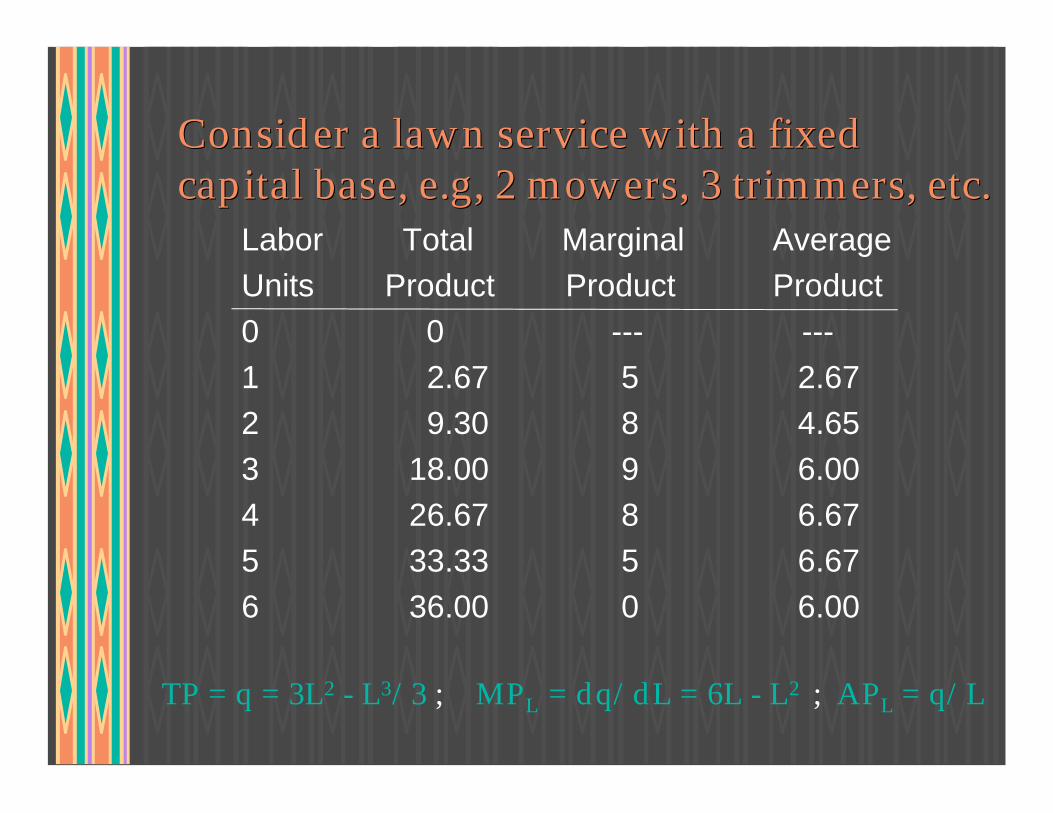
Consider a lawn service with a fixedConsider a lawn service with a fixedcapital base, e.g, 2 mowers, 3 trimmers, etc.capital base, e.g, 2 mowers, 3 trimmers, etc.

Labor Total Marginal AverageUnits Product Product Product0 0 --- ---1 2.67 5 2.672 9.30 8 4.653 18.00 9 6.004 26.67 8 6.675 33.33 5 6.676 36.00 0 6.00

MPL = dq/dL = 6L - L2 ; APL = q/LTP = q = 3L2 - L3/3 ;

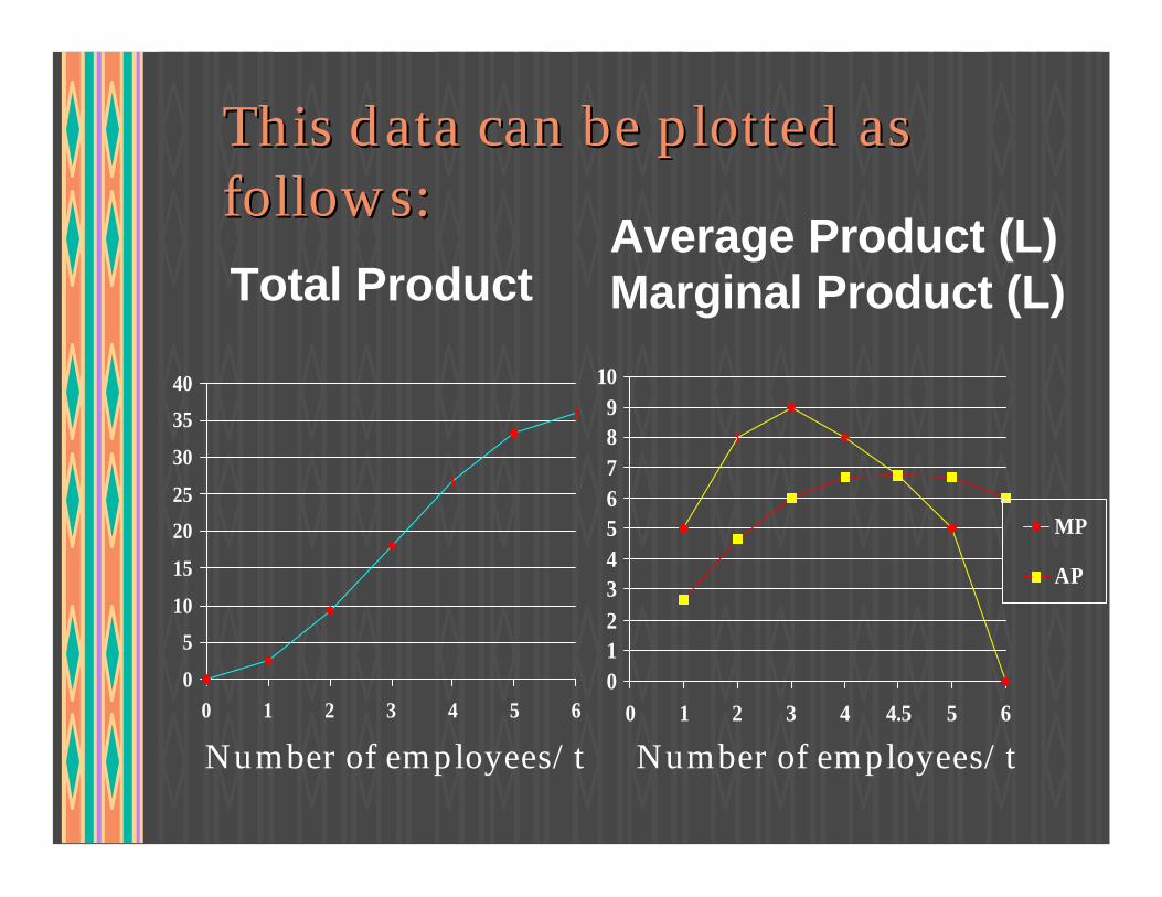
This data can be plotted asThis data can be plotted asfollows:follows:

0

5

10

15

20

25

30

35

40

0 1 2 3 4 5 6

Total Product

0123456789

10

0 1 2 3 4 4.5 5 6

MP

AP

Average Product (L)Marginal Product (L)

Number of employees/t Number of employees/t

The Law of DiminishingThe Law of DiminishingReturnsReturns

uu After a certain point, whenAfter a certain point, whenadditional units of a variable inputadditional units of a variable inputare added to fixed inputs, theare added to fixed inputs, themarginal product of the variablemarginal product of the variableinput declinesinput declines

uu At this point, output startsAt this point, output startsincreasing at a decreasing rateincreasing at a decreasing rate

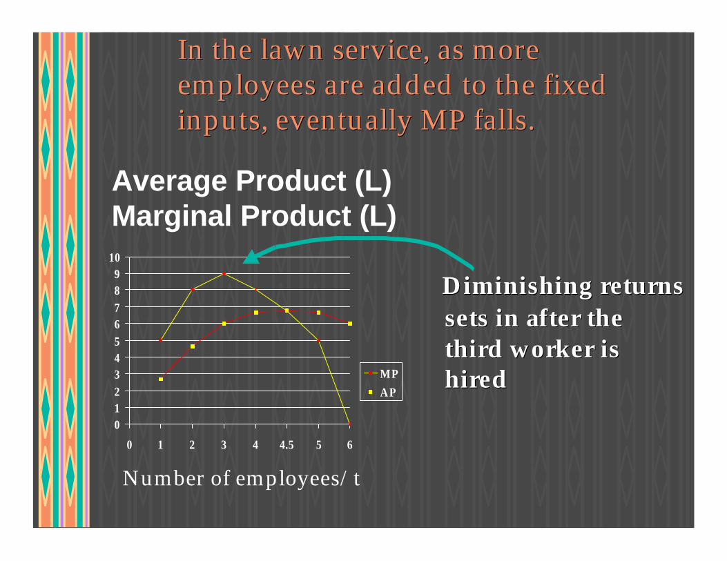
In the lawn service, as moreIn the lawn service, as moreemployees are added to the fixedemployees are added to the fixedinputs, eventually MP falls.inputs, eventually MP falls.

Diminishing returnsDiminishing returnssets in after thesets in after thethird worker isthird worker ishiredhired

0123456789

10

0 1 2 3 4 4.5 5 6

MP

AP

Number of employees/t

Average Product (L)Marginal Product (L)

Adding More Inputs to theAdding More Inputs to theVariable Input Makes the VariableVariable Input Makes the VariableInput More ProductiveInput More Productive

uu More, or better tools makes Labor moreMore, or better tools makes Labor moreproductiveproductive

uu An increase in capital stock increases:An increase in capital stock increases:vv the total product of laborthe total product of laborvv the average product of laborthe average product of laborvv the marginal product of laborthe marginal product of labor

Returning to our lawn service, supposeReturning to our lawn service, supposethe owners can invest in four mowersthe owners can invest in four mowersrather than tworather than two

Units of Two Mowers Four MowersUnits of Two Mowers Four MowersLabor TP MP TP MPLabor TP MP TP MP 0 0 --- 0 --- 0 0 --- 0 --- 1 2.67 5 3.67 7 1 2.67 5 3.67 7 2 9.30 8 13.33 12 2 9.30 8 13.33 12 3 18.00 9 27.00 15 3 18.00 9 27.00 15 4 26.67 8 42.67 16 4 26.67 8 42.67 16 5 33.33 5 58.33 15 5 33.33 5 58.33 15 6 36.00 0 72.00 12 6 36.00 0 72.00 12

With 4 mowers, q = 4L2 - L3/3 ; MPL = 8L - L2

Review: The ProductionReview: The ProductionFunctionFunctionuu Simplifying Assumptions we useSimplifying Assumptions we use

vv Short Run, therefore at least one input isShort Run, therefore at least one input isfixedfixed

vv Output, q, depends on only two inputsOutput, q, depends on only two inputsuu Labor, L, the variable inputLabor, L, the variable inputuu Capital, K, the fixed inputCapital, K, the fixed input

uu As the variable input is added to the fixedAs the variable input is added to the fixedinput, q increases first at an increasing rate, butinput, q increases first at an increasing rate, butultimately at a decreasing rate due to the law ofultimately at a decreasing rate due to the law ofdiminishing marginal returnsdiminishing marginal returns

uu More of the fixed inputs make the variableMore of the fixed inputs make the variableinputs more productiveinputs more productive

L1

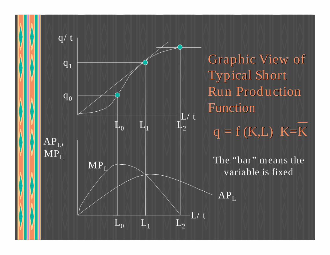
Graphic View ofGraphic View ofTypical ShortTypical ShortRun ProductionRun ProductionFunctionFunction

q = f (K,L) K=Kq = f (K,L) K=KL2L0

q0

q1

q/t

APL

APL,MPL

MPL

L/t

L/tL0 L1 L2

The “bar” means thevariable is fixed

L1

First, notice theFirst, notice thetotal producttotal productcurve. Output ascurve. Output asa function ofa function oflabor depends onlabor depends ona given fixeda given fixedcapital input.capital input.With more K,With more K,labor is morelabor is moreproductiveproductive

L2L0

q0

q1

q/t

L/t

More capital makes labormore productive

q with K = K1

q with K = K2 > K1

L1

Second, find MPSecond, find MPby taking theby taking theslope of TPslope of TP

L2L0

q0

q1

q/t

MPL

MPL

L/t

L/tL0 L1 L2

A

BC

At “A” , the inflectionpoint, the slope ismaximized; The law ofdiminishing returns setin

at “B”, the slope alsoequals the averageproduct;

at “C”, the slope is zero

L1

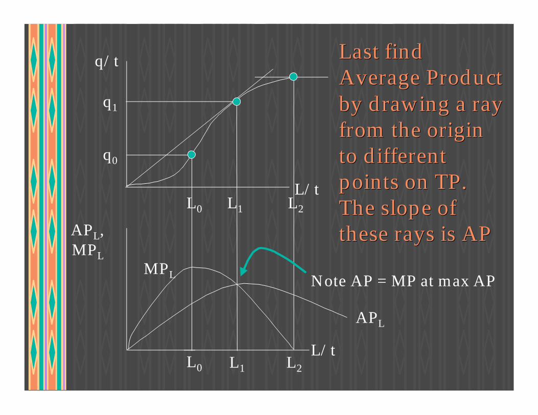
Last findLast findAverage ProductAverage Productby drawing a rayby drawing a rayfrom the originfrom the originto differentto differentpoints on TP.points on TP.The slope ofThe slope ofthese rays is APthese rays is AP

L2L0

q0

q1

q/t

APL

APL,MPL

MPL

L/t

L/tL0 L1 L2

Note AP = MP at max AP

L1

EverythingEverythingTogether: TypicalTogether: TypicalShort RunShort RunProductionProductionFunctionFunction

q = f (K,L) K=Kq = f (K,L) K=KL2L0

q0

q1

q/t

APL

APL,MPL

MPL

L/t

L/tL0 L1 L2

The “bar” means thevariable is fixed

The Equal MP/P RuleThe Equal MP/P Ruleuu A necessary condition for minimizing cost ofA necessary condition for minimizing cost of

any given level of an activity is to mix theany given level of an activity is to mix thevariable inputs such that their Marginalvariable inputs such that their MarginalProduct/Price ratios (MPProduct/Price ratios (MPii/P/Pii) are equal) are equal

uu MPMP11/P/P11 = MP = MP22/P/P22 = . . . = MP = . . . = MPnn/P/Pnn for all n for all nvariable inputsvariable inputs

uu If MPIf MP11/P/P11 > MP > MP22/P/P22 you are getting more you are getting morevalue per dollar from input 1 than from inputvalue per dollar from input 1 than from input2 and to produce the same level of output at2 and to produce the same level of output atlower cost you should hire more 1 and less 2lower cost you should hire more 1 and less 2

uu As you hire more of input 1, MPAs you hire more of input 1, MP11 falls, and as falls, and asyou hire less of input 2, MPyou hire less of input 2, MP22 increases increases

From the Short Run to theFrom the Short Run to theLong RunLong Runuu In the short run at least one input isIn the short run at least one input is

fixedfixeduu In the long run all inputs may beIn the long run all inputs may be

changedchangeduu An important property of theAn important property of the

production function is its “Internalproduction function is its “InternalReturns to Scale”Returns to Scale”

Types of Internal Returns to ScaleTypes of Internal Returns to Scale

uu Economies of ScaleEconomies of Scale: a proportional: a proportionalchange in change in allall inputs leads to a larger inputs leads to a largerproportional change in outputproportional change in output

uu Constant Returns to ScaleConstant Returns to Scale: a: aproportional change in proportional change in allall inputs leads inputs leadsto an equal proportional change into an equal proportional change inoutputoutput

uu Diseconomies of ScaleDiseconomies of Scale: a proportional: a proportionalchange in change in allall inputs leads to a smaller inputs leads to a smallerproportional change in outputproportional change in output

Returns to ScaleReturns to Scaleuu Changing all inputs in the same proportion isChanging all inputs in the same proportion is

a “scale” change, e.g., increase all by 10%,a “scale” change, e.g., increase all by 10%,decrease all by 5%decrease all by 5%

uu Increasing Returns to Scale: %Increasing Returns to Scale: %ÎÎq>%q>%ÎÎRRuu Constant Returns to Scale: % Constant Returns to Scale: % ÎÎq=%q=%ÎÎRRuu Decreasing Returns to Scale: %Decreasing Returns to Scale: %ÎÎq<%q<%ÎÎRR

(where R is all resources)(where R is all resources)uu As we will see, cost curves in the long run areAs we will see, cost curves in the long run are

based on the underlying productionbased on the underlying productiontechnology, i.e., returns to scaletechnology, i.e., returns to scale

Returns to Scale, examplesReturns to Scale, examples

uu IRTS: doubling all inputs leads to anIRTS: doubling all inputs leads to anincrease of 125% in qincrease of 125% in q

uu DRTS: an increase in all inputs by 5%DRTS: an increase in all inputs by 5%leads to a 3% increase in qleads to a 3% increase in q

uu CRTS: a decrease in all inputs by 10%CRTS: a decrease in all inputs by 10%lead to a 10% fall in qlead to a 10% fall in q

uu If all inputs are decreased by 5% andIf all inputs are decreased by 5% andoutput falls by 7%, %output falls by 7%, %ÎÎq>%q>%ÎÎR, thereforeR, thereforeIRTSIRTS

What if all inputs change butWhat if all inputs change butnot in the same proportion?not in the same proportion?

uu If the %If the %ÎÎq>%q>%ÎÎCosts we use the termCosts we use the termEconomies of ScaleEconomies of Scale

uu If the %If the %ÎÎq<%q<%ÎÎCosts we use the termCosts we use the termDiseconomies of ScaleDiseconomies of Scale

uu IRTS implies Economies of Scale butIRTS implies Economies of Scale butEconomies of scale do not imply IRTSEconomies of scale do not imply IRTS

uu The same is true for the relationshipThe same is true for the relationshipbetween Diseconomies of Scale and DRTSbetween Diseconomies of Scale and DRTS

Economies of ScaleEconomies of Scale

uu Reasons for economies of scaleReasons for economies of scaleuu Greater specialization of resourcesGreater specialization of resources

vv Divide work get benefits of specialization (lower costs).Divide work get benefits of specialization (lower costs).This was the point emphasized by Adam SmithThis was the point emphasized by Adam Smith

vv Efficient Utilization of specialized technologies may notEfficient Utilization of specialized technologies may notbe possible at small scale, e.g., Airline hubs, irrigationbe possible at small scale, e.g., Airline hubs, irrigationsystemssystems

vv Arithmetic relationships, e.g.,Arithmetic relationships, e.g.,uu the circumference of a pipe, which approximatesthe circumference of a pipe, which approximates

cost equals pi*2*radius, but the carrying capacitycost equals pi*2*radius, but the carrying capacitydepends on the area which equals pi*radius squareddepends on the area which equals pi*radius squared

Diseconomies of ScaleDiseconomies of Scaleuu Reasons for diseconomies of scaleReasons for diseconomies of scaleuu Coordination and control problems as firmCoordination and control problems as firm

gets large--The Principal/Agent Problemgets large--The Principal/Agent Problemvv The Principal is the person in charge and theThe Principal is the person in charge and the

Agent is the person charged with carrying outAgent is the person charged with carrying outthe wishes of the Principalthe wishes of the Principal

vv Two conditions need to be present for the P/ATwo conditions need to be present for the P/Aproblem to existproblem to exist

uu Agents and Principals must have differentAgents and Principals must have differentobjectivesobjectives

uu It must be costly for the Principal to monitor andIt must be costly for the Principal to monitor andenforceenforce

Now, let’s link production toNow, let’s link production tocostscosts

uu Each production relationship has a costEach production relationship has a costcounterpartcounterpartvv TP:variable inputTP:variable input -- Variable Cost-- Variable Costvv AP:variable input AP:variable input -- Average Variable Cost-- Average Variable Costvv MP:variable input MP:variable input -- Marginal Cost-- Marginal Costvv Fixed inputsFixed inputs -- Fixed (or Sunk) Cost-- Fixed (or Sunk) Costvv MP/P rule MP/P rule -- Equal MC rule-- Equal MC rule

uu The production function and the MP/P ruleThe production function and the MP/P ruletells us the minimum cost of producing anytells us the minimum cost of producing anylevel of output, q: Cost = input price *inputslevel of output, q: Cost = input price *inputsrequiredrequired

The End The End

Go Ahead to Part III, on Costs