The Sum of All FEARS Investor Sentiment and Asset Priceszda/FEARS.pdf · The Sum of All FEARS Investor Sentiment and Asset Prices ... Rady School of Management, ... (FEARS) index

[11:32 28/10/2014 RFS-hhu072.tex] Page: 1 1–34

The Sum of All FEARS Investor Sentimentand Asset Prices

Zhi DaMendoza College of Business, University of Notre Dame

Joseph EngelbergRady School of Management, University of California at San Diego

Pengjie GaoMendoza College of Business, University of Notre Dame

We use daily Internet search volume from millions of households to reveal market-levelsentiment. By aggregating the volume of queries related to household concerns (e.g.,“recession,” “unemployment,” and “bankruptcy”), we construct a Financial and EconomicAttitudes Revealed by Search (FEARS) index as a new measure of investor sentiment.Between 2004 and 2011, we find FEARS (i) predict short-term return reversals, (ii) predicttemporary increases in volatility, and (iii) predict mutual fund flows out of equity funds andinto bond funds. Taken together, the results are broadly consistent with theories of investorsentiment. (JEL G10)

John Maynard Keynes (1936) argued that markets can fluctuate wildly underthe influence of investors’ “animal spirits,” which move prices in a wayunrelated to fundamentals. Fifty years later, De Long, Shleifer, Summers, andWaldmann (1990; DSSW hereafter) formalized the role of investor sentimentin financial markets. DSSW demonstrate that if uninformed noise traders basetheir trading decisions on sentiment and risk-averse arbitrageurs encounterlimits to arbitrage, sentiment changes will lead to more noise trading, greatermispricing, and excess volatility. Although the survival of noise traders in thelong run remains open for debate (e.g., Kogan, Ross, Wang and Westerfield2006, 2009), there is a growing consensus that noise traders can induce large

We thank Nick Barberis, Shane Corwin, Jennifer Conrad, David Hirshleifer (the editor), Bob Jennings, ShimonKogan, Ralph Koijen, Owen Lamont, Paul Schultz, Andrei Shleifer, Paul Tetlock, Dick Thaler, Jeff Wurgler, YuYuan, two anonymous referees and seminar participants at University of Notre Dame, State of Indiana AnnualConference, the 2010 NBER Behavioral Economics meeting and the WFA 2010 meeting for helpful commentsand discussions. We are grateful to Conrad Gann at TrimTabs, Inc. for his assistance with the daily mutual funddata used in this study, Shane Corwin for providing us with the intraday data for realized volatility calculationduring the recent years, and Pavel Savor for sharing with us macro announcement dates. Jianfeng Zhu providedvaluable research assistance. We are responsible for remaining errors. Send correspondence to Joseph Engelberg,Finance Department, UCSD Rady School of Management, 9500 Gilman Drive #0553, La Jolla, CA 92093-0553;telephone: 858-822-7912. E-mail: [email protected].

© The Author 2014. Published by Oxford University Press on behalf of The Society for Financial Studies.All rights reserved. For Permissions, please e-mail: [email protected]:10.1093/rfs/hhu072

RFS Advance Access published November 13, 2014 at U

niversity of Notre D

ame on N

ovember 18, 2014

http://rfs.oxfordjournals.org/D

ownloaded from

http://rfs.oxfordjournals.org/

[11:32 28/10/2014 RFS-hhu072.tex] Page: 2 1–34

The Review of Financial Studies / v 0 n 0 2014

price movements and excess volatility in the short run.1 As Baker and Wurgler(2007) put it in their survey article: “Now, the question is no longer, as it wasa few decades ago, whether investor sentiment affects stock prices, but ratherhow to measure investor sentiment and quantify its effects.”

In this paper we propose a possible answer: investor sentiment can be directlymeasured through the Internet search behavior of households. We aggregatethe volume of Internet search queries such as “recession,” “bankruptcy,” and“unemployment” from millions of U.S. households to construct a Financial andEconomic Attitudes Revealed by Search (FEARS) index. We then quantify theeffects of FEARS on asset prices, volatility, and fund flows. We find that FEARSpredict return reversals: although increases in FEARS correspond with lowmarket-level returns today, they predict high returns (reversal) over the next fewdays. Moreover, increases in FEARS coincide with only temporary increases inmarket volatility and predict mutual fund flow out of equity funds and into bondfunds. Such trading patterns and price reversals can also come from liquidityshocks, as modeled in Campbell, Grossman and Wang (1993; CGW hereafter).In this case, high-frequency investor sentiment, as measured by FEARS, turnsout to be a powerful trigger of liquidity shocks that affect prices.

The appeal of our search-based sentiment measure is more transparentwhen compared with alternatives. Traditionally, empiricists have taken twoapproaches to measuring investor sentiment. Under the first approach,empiricists proxy for investor sentiment with market-based measures suchas trading volume, closed-end fund discount, initial public offering (IPO)first-day returns, IPO volume, option implied volatilities (VIX), or mutualfund flows (see Baker and Wurgler (2007) for a comprehensive survey ofthe literature). Although market-based measures have the advantage of beingreadily available at a relatively high frequency, they have the disadvantage ofbeing the equilibrium outcome of many economic forces other than investorsentiment. Qiu and Welch (2006) put it succinctly: “How does one test a theorythat is about inputs → outputs with an output measure?”

Under the second approach, empiricists use survey-based indices such as theUniversity of Michigan Consumer Sentiment Index, the UBS/GALLUP Indexfor Investor Optimism, or investment newsletters (Brown and Cliff (2005),Lemmon and Portniaguina (2006), and Qiu and Welch (2006)). Comparedwith survey-based measures of investor sentiment, the search-based sentimentmeasure we propose has several advantages. First, search-based sentimentmeasures are available at a high frequency.2 Survey measures are often available

1 A particularly interesting thread of this literature examines sentiment following non-economic events such assports (Edmans, Garcia, and Norli 2007), aviation disasters (Kaplanski and Levy 2010), weather conditions(Hirshleifer and Shumway 2003), and seasonal affective disorder (SAD; Kamstra, Kramer, and Levi 2003), andshows these sentiment-changing events cause changes in asset prices.

2 To date, high-frequency analysis of investor sentiment is found only in laboratory settings. For example,Bloomfield, O’Hara, and Saar (2009) use laboratory experiments to investigate the impact of uninformed traderson underlying asset prices.

2

at University of N

otre Dam

e on Novem

ber 18, 2014http://rfs.oxfordjournals.org/

Dow

nloaded from


[11:32 28/10/2014 RFS-hhu072.tex] Page: 3 1–34

The Sum of All FEARS Investor Sentiment and Asset Prices

monthly or quarterly. In fact, we find that our daily FEARS index can predictmonthly survey results of consumer confidence and investor sentiment. Second,search-based measures reveal attitudes rather than inquire about them.Althoughmany people answer survey questions for altruistic reasons, there is often littleincentive to answer survey questions carefully or truthfully, especially whenquestions are sensitive (Singer 2002). Search volume has the potential to revealmore personal information where non-response rates in surveys are particularlyhigh or the incentive for truth-telling is low. For example, eliciting the likelihoodof job loss via survey may be a sensitive topic for a respondent. On the otherhand, aggregate search volume for terms like “find a job,” “job search,” or“unemployment” reveals concern about job loss. Finally, some economistshave been skeptical about answers in survey data that are not “cross-verif(ied)with data on actual (not self-reported) behavior observed by objective externalmeasurement” (Lamont, quoted in Vissing-Jorgensen 2003). Search behavioris an example of such objective, external verification.

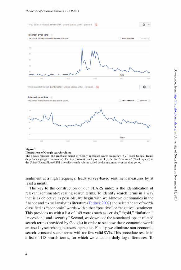
Google, the largest search engine in the world, makes public theSearch Volume Index (SVI) of search terms via its product Google Trends(http://www.google.com/trends/).3 When a user inputs a search term intoGoogle Trends, the application returns the search volume history for that termscaled by the time-series maximum (a scalar). As an example, Figure 1 plotsthe SVI for the terms “recession” and “bankruptcy,” respectively. The plotsconform with intuition. For example, the SVI for “recession” began rising inthe middle of 2007 and then increased dramatically beginning in 2008. Allof this was well before the National Bureau of Economic Research (NBER)announced in December 2008 that the United States had been in a recessionsince December of 2007. The SVI for “bankruptcy” peaks once during 2005and once again during 2009 before falling off. According to the AmericanBankruptcy Institute, actual bankruptcies in the United States follow a similarpattern with peaks in 2005 and 2009/2010.4

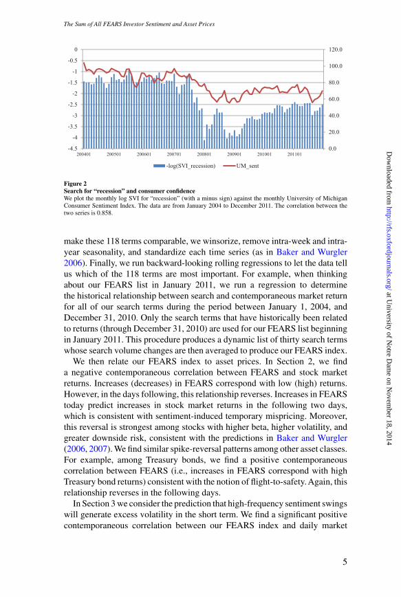
At the monthly frequency, SVI correlates well with alternative measuresof market sentiment. For example, Figure 2 plots the monthly log SVI for“recession” (with a minus sign because higher SVI on “recession” signalspessimism) against the monthly University of Michigan Consumer SentimentIndex (MCSI), which asks households about their economic outlook. Duringour sample period from January 2004 to December 2011, the two time seriesare highly correlated with a correlation coefficient of 0.858. When we use thelog change in “recession” SVI this month to predict next month’s log changein the MCSI, we find that an increase in SVI predicts a decrease in the MCSI(t-value = 2.56). This predictive result suggests that SVI, revealing household

3 By February 2009, Google accounted for 72.11% of all search queries performed in the United States, accordingto Hitwise, which specializes in tracking Internet traffic.

4 See http://www.abiworld.org/AM/AMTemplate.cfm?Section=Home&CONTENTID=65139&TEMPLATE=/CM/ContentDisplay.cfm.

3

at University of N

otre Dam

e on Novem


Dow

nloaded from


[11:32 28/10/2014 RFS-hhu072.tex] Page: 4 1–34


Figure 1Illustrations of Google search volumeThe figures represent the graphical output of weekly aggregate search frequency (SVI) from Google Trends(http://www.google.com/trends/). The top (bottom) panel plots weekly SVI for “recession” (“bankruptcy”) inthe United States. Plotted SVI is weekly search volume scaled by the maximum over the time period.

sentiment at a high frequency, leads survey-based sentiment measures by atleast a month.

The key to the construction of our FEARS index is the identification ofrelevant sentiment-revealing search terms. To identify search terms in a waythat is as objective as possible, we begin with well-known dictionaries in thefinance and textual analytics literature (Tetlock 2007) and select the set of wordsclassified as “economic” words with either “positive” or “negative” sentiment.This provides us with a list of 149 words such as “crisis,” “gold,” “inflation,”“recession,” and “security.” Second, we download the associated top ten relatedsearch terms (provided by Google) in order to see how these economic wordsare used by search engine users in practice. Finally, we eliminate non-economicsearch terms and search terms with too few valid SVIs. This procedure results ina list of 118 search terms, for which we calculate daily log differences. To

4

at University of N

otre Dam

e on Novem


Dow

nloaded from


[11:32 28/10/2014 RFS-hhu072.tex] Page: 5 1–34


0.0

20.0

40.0

60.0

80.0

100.0

120.0

-4.5

-4

-3.5

-3

-2.5

-2

-1.5

-1

-0.5

0

200401 200501 200601 200701 200801 200901 201001 201101

-log(SVI_recession) UM_sent

Figure 2Search for “recession” and consumer confidenceWe plot the monthly log SVI for “recession” (with a minus sign) against the monthly University of MichiganConsumer Sentiment Index. The data are from January 2004 to December 2011. The correlation between thetwo series is 0.858.

make these 118 terms comparable, we winsorize, remove intra-week and intra-year seasonality, and standardize each time series (as in Baker and Wurgler2006). Finally, we run backward-looking rolling regressions to let the data tellus which of the 118 terms are most important. For example, when thinkingabout our FEARS list in January 2011, we run a regression to determinethe historical relationship between search and contemporaneous market returnfor all of our search terms during the period between January 1, 2004, andDecember 31, 2010. Only the search terms that have historically been relatedto returns (through December 31, 2010) are used for our FEARS list beginningin January 2011. This procedure produces a dynamic list of thirty search termswhose search volume changes are then averaged to produce our FEARS index.

We then relate our FEARS index to asset prices. In Section 2, we finda negative contemporaneous correlation between FEARS and stock marketreturns. Increases (decreases) in FEARS correspond with low (high) returns.However, in the days following, this relationship reverses. Increases in FEARStoday predict increases in stock market returns in the following two days,which is consistent with sentiment-induced temporary mispricing. Moreover,this reversal is strongest among stocks with higher beta, higher volatility, andgreater downside risk, consistent with the predictions in Baker and Wurgler(2006, 2007). We find similar spike-reversal patterns among other asset classes.For example, among Treasury bonds, we find a positive contemporaneouscorrelation between FEARS (i.e., increases in FEARS correspond with highTreasury bond returns) consistent with the notion of flight-to-safety. Again, thisrelationship reverses in the following days.

In Section 3 we consider the prediction that high-frequency sentiment swingswill generate excess volatility in the short term. We find a significant positivecontemporaneous correlation between our FEARS index and daily market

5

at University of N

otre Dam

e on Novem


Dow

nloaded from


[11:32 28/10/2014 RFS-hhu072.tex] Page: 6 1–34


volatility measured as either realized volatility on the S&P 500 exchange tradedfund (ETF) return or the Chicago Board of Exchange (CBOE) market volatilityindex (VIX). As volatility displays seasonal patterns and is well known tobe persistent and long-lived (Engel and Patton 2001; Andersen, Bollerslev,Diebold and Ebens 2001; Andersen, Bollerslev, Diebold, and Labys 2003),we account for this long-range dependence through the fractional integratedautoregressive moving average (ARFIMA) model, ARFIMA(1,d,1). Inaddition, parallel to our earlier analysis, we also examine the daily returnson a tradable volatility-based asset, the CBOE VIX futures contract. When werelate our FEARS index to these daily VIX futures returns, we first confirmthe strong contemporaneous correlation between our FEARS index and VIXfutures returns. As before, we find that our FEARS index predicts a reversal inVIX futures returns during the next two trading days.

As a more direct test of the “noise trading” hypothesis, we examine dailymutual fund flows in Section 4. Because individual investors hold about 90%of total mutual fund assets and they are more likely to be “noise” traders, dailyflows to mutual fund groups likely aggregate “noise” trading at the asset classlevel.5 We examine two groups of mutual funds that specialize in equity andintermediate Treasury bonds. We document strong persistence in fund flowsand again use the ARFIMA model to extract daily innovations to these fundflows. Our results suggest significant outflow from the equity market one dayafter an increase in FEARS. We also observe a significant inflow to bond fundsone day after a significant withdrawal from equity funds. Taken together, theevidence indicates a “flight to safety,” with investors shifting their investmentsfrom equities to bonds after a spike in FEARS.

1. Data and Methodology

Although the data for this study come from a variety of sources, we begin bydiscussing the construction of our FEARS index, which is the main variable inour analysis.

1.1 Construction of FEARS indexOur objective is to build a list of search terms that reveal sentimenttoward economic conditions. We follow the recent text analytics literaturein finance, which uses the Harvard IV-4 Dictionary and the Lasswell ValueDictionary (Tetlock 2007; Tetlock, Saar-Tsechansky, and Macskassy 2008).These dictionaries place words into various categories such as “positive,”“negative,” “weak,” “strong,” and so on. Because we are interested in householdsentiment toward the economy, we select the set of words that are “economic”

5 Source: 2007 Investment Company Fact Book by the Investment Company Institute.

6

at University of N

otre Dam

e on Novem


Dow

nloaded from


[11:32 28/10/2014 RFS-hhu072.tex] Page: 7 1–34


words that also have either “positive” or “negative” sentiment.6 This resultsin 149 words such as “bankruptcy,” “crisis,” “gold,” “inflation,” “recession,”“valuable,” and “security.”

We call this list the “primitive” word list. Our next task is to understand howthese words might be searched in Google by households. To do this, we inputeach primitive word into Google Trends, which, among other things, returnsten “top searches” related to each primitive word.7 For example, a search for“deficit” results in the related searches “budget deficit,” “attention deficit,”“attention deficit disorder,” “trade deficit,” and “federal deficit” because thisis how the term “deficit” is commonly searched in Google. Our 149 primitivewords generate 1,490 related terms, which become 1,245 terms after removingduplicates.

Next we remove terms with insufficient data. Of our 1,245 terms, only622 have at least 1,000 observations of daily data.8 Finally, we removeterms that are not clearly related to economics or finance. For example, asearch for “depression” results in the related searches “the depression,” “greatdepression,” “the great depression,” “depression symptoms,” “postpartumdepression,” “depression signs,” etc. We keep the first three terms (which relateto an economic depression) and remove the last three terms (which relate tothe mental disorder of depression). This leaves us with 118 search terms.

We download the SVI for each of these 118 terms over our sample period ofJanuary 2004 to December 2011 from Google Trends. Google Trends allowsusers to restrict SVI results to specific countries (e.g., search volume for“recession” from British households). Because most of the dependent variablesof interest in this paper are related to U.S. indices, we restrict the SVI resultsto the United States. Thus, the measures we construct represent the sentimentof American households. W define the daily change in search term j as:

�SV Ij,t =ln(SV Ij,t

)−ln(SV Ij,t−1). (1)

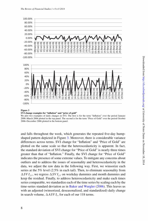
Figure 3 plots the daily log changes for two terms, “Inflation” and “Priceof Gold,” during two different quarters in 2006. The figures demonstrateseveral important features of the search data. The first is seasonality: SVIchange rises during the beginning of the week (e.g., Monday and Tuesday)

6 Specifically, from http://www.wjh.harvard.edu/˜inquirer/spreadsheet_guide.htm we take all economic words(those with tags “Econ@” or “ECON”) which also have a positive or negative sentiment tag (those with tags“Ngtv,” “Negativ,” “Positiv,” or “Pstv”).

7 According to Google, “Top searches refers to search terms with the most significant level of interest. These termsare related to the term you’ve entered. . . . Our system determines relativity by examining searches that havebeen conducted by a large group of users preceding the search term you’ve entered, as well as after.”

8 To increase the response speed, Google currently calculates SVI from a random subset of the actual historicalsearch data. This is why SVIs on the same search term might be slightly different when they are downloaded atdifferent points in time. We believe that the impact of such sampling error is small for our study and should biasagainst finding significant results. As in Da, Gao, and Engelberg (2011), when we download the SVIs severaltimes and compute their correlation, we find that the correlations are usually above 97%.

7

at University of N

otre Dam

e on Novem


Dow

nloaded from


[11:32 28/10/2014 RFS-hhu072.tex] Page: 8 1–34


-100.00%-80.00%-60.00%-40.00%-20.00%0.00%20.00%40.00%60.00%80.00%100.00%

04-Ja

n-06

07-Ja

n-06

10-Ja

n-06

13-Ja

n-06

16-Ja

n-06

19-Ja

n-06

22-Ja

n-06

25-Ja

n-06

28-Ja

n-06

31-Ja

n-06

03-Feb

-06

06-Feb

-06

09-Feb

-06

12-Feb

-06

15-Feb

-06

18-Feb

-06

21-Feb

-06

24-Feb

-06

27-Feb

-06

02-M

ar-06

05-M

ar-06

08-M

ar-06

11-M

ar-06

14-M

ar-06

17-M

ar-06

20-M

ar-06

23-M

ar-06

26-M

ar-06

29-M

ar-06

-100%-80%-60%-40%-20%0%20%40%60%80%100%

03-Oct-06

06-Oct-06

09-Oct-06

12-Oct-06

15-Oct-06

18-Oct-06

21-Oct-06

24-Oct-06

27-Oct-06

30-Oct-06

02-Nov-06

05-Nov-06

08-Nov-06

11-Nov-06

14-Nov-06

17-Nov-06

20-Nov-06

23-Nov-06

26-Nov-06

29-Nov-06

02-Dec-06

05-Dec-06

08-Dec-06

11-Dec-06

14-Dec-06

17-Dec-06

20-Dec-06

23-Dec-06

26-Dec-06

29-Dec-06

Figure 3SVI change examples for “inflation” and “price of gold”We plot two examples of daily changes in SVI. The first is for the term “Inflation” over the period January2006–March 2006 plotted in the top panel. The second is for the term “Price of Gold” over the period October2006–December 2006 plotted in the bottom panel.

and falls throughout the week, which generates the repeated five-day hump-shaped pattern depicted in Figure 3. Moreover, there is considerable variancedifferences across terms. SVI change for “Inflation” and “Price of Gold” areplotted on the same scale so that the heteroscedasticity is apparent. In fact,the standard deviation of SVI change for “Price of Gold” is nearly three timesgreater than that of “Inflation.” Finally, the SVI change for “Price of Gold”indicates the presence of some extreme values. To mitigate any concerns aboutoutliers and to address the issues of seasonality and heteroscedasticity in thedata, we adjust the raw data in the following way. First, we winsorize eachseries at the 5% level (2.5% in each tail). Then, to eliminate seasonality from�SV Ij,t , we regress �SV Ij,t on weekday dummies and month dummies andkeep the residual. Finally, to address heteroscedasticity and make each timesseries comparable, we standardize each of the time series by scaling each by thetime-series standard deviation as in Baker and Wurgler (2006). This leaves uswith an adjusted (winsorized, deseasonalized, and standardized) daily changein search volume, �ASV It , for each of our 118 terms.

8

at University of N

otre Dam

e on Novem


Dow

nloaded from


[11:32 28/10/2014 RFS-hhu072.tex] Page: 9 1–34


Our final step is to let the data identify search terms that are most important forreturns. To do this we run expanding backward rolling regressions of �ASV I

on market returns every six months (every June and December) to determinethe historical relationship between search and contemporaneous market returnfor all 118 of our search terms. When we do this it becomes clear that, givena search term that has a strong relationship with the market, the relationship isalmost always negative. This is despite the fact that we began with economicwords of both positive and negative sentiment when selecting words from theHarvard and Lasswell dictionaries. For example, when we use all 118 termsin the full sample (January 2004–December 2011) we find zero terms with at-statistic on �ASV I above 2.5 but fourteen terms with a t-statistic below−2.5. These terms include “recession,” “great depression,” “gold price,” and“crisis.” As in Tetlock (2007) it appears that negative terms in English languageare most useful for identifying sentiment. For this reason, we use only the termsthat have the largest negative t-statistic on �ASV I to form our FEARS index.Formally, we define FEARS on day t as:

FEARSt =30∑i=1

Ri(�ASV It ) (2)

where Ri(�ASV It ) is the �ASV It for the search term that had a t-statisticrank of i from the period January 2004 through the most recent six-monthperiod, where ranks run from smallest (i =1) to largest (i =118). For example,at the end of June 2009, we run a regression of �ASV I on contemporaneousmarket return during the period January 1, 2004–June 30, 2009, for each of our118 search terms. Then we rank the t-statistic on �ASV I from this regressionfrom most negative (i =1) to most positive (i =118). We select the thirty mostnegative terms and use these terms to form our FEARS index for the periodfrom July 1, 2009, to December 31, 2009. FEARS on day t during this period issimply the average �ASV I of these thirty terms on day t . Given our relativelyshort sample period, we choose an expanding rolling window to maximize thestatistical power of the selection. We choose a cutoff of thrity as it is oftenconsidered to be the minimum number of observations needed to diversifyaway idiosyncratic noise. Robustness to alternative cutoff choices (e.g., toptwenty-five or top thirty-five) is shown in Table 5. Finally, due to the need foran initial window of at least six months, our FEARS index starts in July 2004.

There are several advantages to this historical, regression-based approach forselecting terms. First, using historical regressions to identify the most relevantterms is an objective way to “let the data speak for itself.” Kogan et al. (2009)also take a similar regression approach to identify relevant words in firm 10-Ksand argue this approach not only helps the researcher identify terms that werenot ex ante obvious but also is an objective way to select terms. This is also truein our case. For example, the word “gold” is considered an economic word ofpositive sentiment by the Harvard dictionary, and yet we find a strong negative

9

at University of N

otre Dam

e on Novem


Dow

nloaded from


[11:32 28/10/2014 RFS-hhu072.tex] Page: 10 1–34


Table 1FEARS terms from the full sample

Search Term T-Statistic

1 GOLD PRICES −6.042 RECESSION −5.603 GOLD PRICE −4.814 DEPRESSION −4.565 GREAT DEPRESSION −4.156 GOLD −3.987 ECONOMY −3.528 PRICE OF GOLD −3.239 THE DEPRESSION −3.2010 CRISIS −2.9311 FRUGAL −2.8712 GDP −2.8513 CHARITY −2.6314 BANKRUPTCY −2.5015 UNEMPLOYMENT −2.4616 INFLATION RATE −2.3217 BANKRUPT −2.2818 THE GREAT DEPRESSION −2.1719 CAR DONATE −2.1120 CAPITALIZATION −2.1021 EXPENSE −1.9722 DONATION −1.8923 SAVINGS −1.8224 SOCIAL SECURITY CARD −1.7125 THE CRISIS −1.6526 DEFAULT −1.6327 BENEFITS −1.5628 UNEMPLOYED −1.5529 POVERTY −1.5230 SOCIAL SECURITY OFFICE −1.51

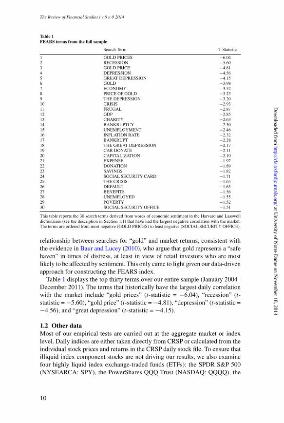
This table reports the 30 search terms derived from words of economic sentiment in the Harvard and Lasswelldictionaries (see the description in Section 1.1) that have had the largest negative correlation with the market.The terms are ordered from most negative (GOLD PRICES) to least negative (SOCIAL SECURITY OFFICE).

relationship between searches for “gold” and market returns, consistent withthe evidence in Baur and Lucey (2010), who argue that gold represents a “safehaven” in times of distress, at least in view of retail investors who are mostlikely to be affected by sentiment. This only came to light given our data-drivenapproach for constructing the FEARS index.

Table 1 displays the top thirty terms over our entire sample (January 2004–December 2011). The terms that historically have the largest daily correlationwith the market include “gold prices” (t-statistic = −6.04), “recession” (t-statistic = −5.60), “gold price” (t-statistic = −4.81), “depression” (t-statistic =−4.56), and “great depression” (t-statistic = −4.15).

1.2 Other dataMost of our empirical tests are carried out at the aggregate market or indexlevel. Daily indices are either taken directly from CRSP or calculated from theindividual stock prices and returns in the CRSP daily stock file. To ensure thatilliquid index component stocks are not driving our results, we also examinefour highly liquid index exchange-traded funds (ETFs): the SPDR S&P 500(NYSEARCA: SPY), the PowerShares QQQ Trust (NASDAQ: QQQQ), the

10

at University of N

otre Dam

e on Novem


Dow

nloaded from


[11:32 28/10/2014 RFS-hhu072.tex] Page: 11 1–34


Russell 1000 Index ETF (NYSEARCA: IWB), and the Russell 2000 Index ETF(NYSEARCA: IWM). We also obtain intraday data on SPY from TAQ in orderto estimate realized market volatility. Finally, we obtain Treasury portfolioreturns from the CRSP ten-year constant maturity Treasury file.

The Chicago Board Options Exchange (CBOE) daily market volatility index(VIX), which measures the implied volatility of options on the S&P 100 stockindex, is well known as an “investor fear gauge” by practitioners. For example,Whaley (2001) discusses the spikes in the VIX series since its 1986 inception,which captures the crash of October 1987 and the 1998 Long Term CapitalManagement crisis. Baker and Wurgler (2007) consider it to be an alternativemarket sentiment measure. We include the VIX index as a control variable inmost specifications. Later we use our FEARS index to predict VIX, as well asreturns from VIX futures traded on the CBOE.

We obtain a high-frequency measure of concurrent macroeconomicconditions from the Federal Reserve Bank of Philadelphia.9 Using a dynamicfactor model to extract the latent state of macroeconomic activity from alarge number of macroeconomic variables, Aruoba, Diebold, and Scotti (2009)construct a daily measure of macroeconomic activities (the “ADS” index).According to the Federal Reserve Bank of Philadelphia, construction of theADSindex includes a battery of seasonally adjusted macroeconomic variables ofmixed frequencies: weekly initial jobless claims; monthly payroll employment,industrial production, personal income less transfer payments, manufacturingand trade sales; and quarterly real gross domestic product (GDP). The changein the ADS index reflects innovations driven by macroeconomic conditions.An increase in the ADS index indicates progressively better-than-averageconditions, while a decrease in the ADS index indicates progressively worse-than-average conditions. We also obtain the dates of important macroeconomicannouncements about consumer price index (CPI), producer price index (PPI),unemployment rates, or interest rates, as in Savor and Wilson (2013), for oursample period.

To capture uncertainty related to economic policies, we adopt a news-basedmeasure of economic policy uncertainty (EPU) recently developed by Baker,Bloom, and Davis (2013).10 This measure is constructed by counting thenumber of U.S. newspaper articles achieved by the NewsBank Access WorldNews database with at least one term from each of the following three categoriesof terms: (i) “economic” or “economy”; (ii) “uncertain” or “uncertainty”; and(iii) “legislation,” “deficit,” “regulation,” “congress,” “Federal Reserve,” or“White House.” Baker, Bloom, and Davis (2013) provide evidence that thenews-based measure of EPU seems to capture perceived economic policyuncertainty.

9 The data are available at http://www.philadelphiafed.org/research-and-data/real-time-center/business-conditions-index.

10 The data are available at http://www.policyuncertainty.com/us_daily.html.

11

at University of N

otre Dam

e on Novem


Dow

nloaded from


[11:32 28/10/2014 RFS-hhu072.tex] Page: 12 1–34


In a robustness table we also use a measure of news-based sentiment. Ournews-based sentiment measure is the fraction of negative words in the WallStreet Journal “Abreast of the Market” column as in Tetlock (2007). To identifynegative words, we follow Tetlock (2007) and use the dictionaries from theGeneral Inquirer program. Loughran and McDonald (2011) argue that somenegative words in these dictionaries do not have a truly negative meaning inthe context of financial markets. For example, words like “tax,” “cost,” “vice,”and “liability” simply describe company operations. Instead, they develop analternative negative word list that better reflects the tone of financial text. Weobtain qualitatively similar results when using either word list.

Our daily mutual fund flow data are obtained from TrimTabs, Inc. Adescription of TrimTabs data can be found in Edelen and Warner (2002) andGreene and Hodges (2002). TrimTabs collects daily flow information for about1,000 distinct mutual funds that represent approximately 20% of the universeof U.S.-based mutual funds according to Greene and Hodges (2002). TrimTabsaggregates the daily flows for groups of mutual funds categorized using fundobjectives from Morningstar. For our study, we focus on the daily flow of twogroups of mutual funds. The first group (Equity) specializes in equity. Thesecond group (MTB) specializes in “intermediate Treasury bonds.” For eachgroup, we compute the daily flow as the ratio between dollar flow (inflow minusoutflow) and fund total net assets (TNA). The data we received from TrimTabscovers the five-year period from July 2004 to October 2009.

2. FEARS and Asset Returns

We first examine the relationship between FEARS and returns across variousasset classes. We then examine how this relationship varies among the cross-section of stocks when we consider limits to arbitrage.

2.1 FEARS and average returnsOne salient feature of sentiment theories is the heterogeneity of investors. Insentiment models, there is typically one class of investors who suffer from abias, such as extrapolative expectations about future cash flows. These biaseslead investors to make demands for assets that are not reflected by fundamentalsand, in the presence of limits to arbitrage, push prices away from fundamentalvalues. Thus, a central prediction of theories of investor sentiment is reversal.For example, when sentiment is high, prices are temporarily high but laterbecome low.

We look for evidence of return reversals by running the followingregressions:

returni,t+k =β0 +β1FEARSt +∑m

γmControlmi,t +ui,t+k. (3)

In regression (3), returni,t+k denotes asset i ’s return on day t +k . We alsoconsider two-day cumulative returns, returni,[t+1,t+2], to gain a perspective

12

at University of N

otre Dam

e on Novem


Dow

nloaded from


[11:32 28/10/2014 RFS-hhu072.tex] Page: 13 1–34


on the cumulative effects of return reversals. Control variables (Controlmi,t )include lagged asset-class returns (up to five lags), changes in a news-basedmeasure of economic policy uncertainty (EPU ), the CBOE volatility index(V IX), and changes in the Aruoba-Diebold-Scotti (ADS) business conditionsindex.11 We calculate bootstrapped standard errors, and our statistical inferenceis conservative.12

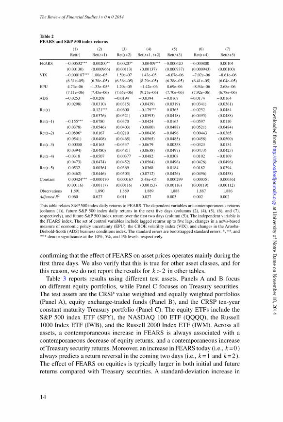
In Table 2, we examine the Standard and Poor’s 500 index. When k =0 ,the negative and significant coefficient on FEARSt suggests a negativecontemporaneous relationship between FEARS and a broad equity index. Daysin which there were sharp declines in the equity indices there were also sharpincreases in search for terms like “recession,” “gold price,” “depression,”and so on. For example, the first column of Table 2 shows that a standard-deviation increase in FEARS corresponds with a contemporaneous declineof 19 basis points for the daily S&P 500 index, after controlling for laggedreturns, contemporaneous V IX, EPU , and ADS.13 This result is perhapsunsurprising. Recall that the search terms that compose the FEARS index wereselected based on their historical correlation with the market. Table 2 suggeststhat they continue to be correlated out of sample.

Much of the day 0 effect, however, is temporary. In the ensuing days,the positive and significant coefficient on FEARS suggests that increases inFEARS predict higher returns. As evident in columns 2 to 4, these reversals aresignificant on both the first and the second days (k =1 and 2).14 Specifically, astandard-deviation increase in FEARS predicts an increase of 7.1 basis pointsin the S&P 500 at k =1 (significant at the 5% level), and an increase of 7.3basis points at k =2 (significant at the 10% level). The cumulative impact of astandard-deviation increase in FEARS predicts a cumulative increase of 14.4basis points in the S&P 500 over days 1 and 2 (significant at the 1% level). Inother words, the initial impact of FEARS on the S&P 500 index on day 0 isalmost completely reversed after two days. In Table 2, we also consider longerhorizons, ranging from k =3 to k =5 , but none of the coefficients on FEARSare statistically significant and point estimates are economically negligible,

11 We also find that replacing the VIX index with an increasingly popular alternative sentiment index, the CreditSuisse Fear Barometer (CSFB), has little effect on the results.

12 For all the empirical results reported in the paper, we have also computed standard errors that are robust toheteroscedasticity and autocorrelations. These unreported standard errors imply even higher t-values in general,and thus only strengthen our conclusions.

13 A one-standard-deviation change in the FEARS index corresponds to 0.3549. Recall that while each individualsearch term has been standardized so that its standard deviation is one by construction, the average across searchterms will not have a standard deviation of one given correlation among search terms.

14 Note that search volume and returns are measured over different intervals. Daily search volume is measured overthe interval 00:00–24:00 PST, while returns are measured over the interval 13:00 PST–13:00 PST. Therefore, thereturn on day t+1 overlaps with some search volume on day t. If FEARS measured after hours on day t spilledinto day t+1 return, we would expect a negative coefficient in column 2. We do not find one, which suggests thatthe effect from this mismatch in measurement of intervals is small. Moreover, FEARS on day t predict returnson day t+2 where there is no overlap of measurement intervals.

13

at University of N

otre Dam

e on Novem


Dow

nloaded from


[11:32 28/10/2014 RFS-hhu072.tex] Page: 14 1–34


Table 2FEARS and S&P 500 index returns

(1) (2) (3) (4) (5) (6) (7)Ret(t) Ret(t+1) Ret(t+2) Ret[t+1, t+2] Ret(t+3) Ret(t+4) Ret(t+5)

FEARS −0.00532∗∗∗ 0.00200∗∗ 0.00207∗ 0.00409∗∗∗ −0.000620 −0.000800 0.00104(0.00130) (0.000966) (0.00113) (0.00137) (0.000937) (0.000943) (0.00100)

VIX −0.000187∗∗∗ 1.80e–05 1.50e–07 1.43e–05 –6.07e–06 –7.02e–06 –8.61e–06(6.31e–05) (6.38e–05) (6.36e–05) (8.29e–05) (6.28e–05) (6.41e–05) (6.04e–05)

EPU 4.73e–06 –1.33e–05* 1.20e–05 –1.42e–06 8.69e–06 –8.94e–06 2.68e–06(7.11e–06) (7.45e–06) (7.65e–06) (9.27e–06) (7.70e–06) (7.92e–06) (6.78e–06)

ADS −0.0253 −0.0208 −0.0194 −0.0394 −0.0168 −0.0174 −0.0164(0.0298) (0.0310) (0.0315) (0.0439) (0.0319) (0.0341) (0.0361)

Ret(t) −0.121∗∗∗ −0.0600 −0.179∗∗∗ 0.0365 −0.0252 −0.0484(0.0376) (0.0521) (0.0595) (0.0418) (0.0495) (0.0488)

Ret(t–1) −0.155∗∗∗ −0.0780 0.0370 −0.0424 −0.0165 −0.0597 0.0110(0.0378) (0.0546) (0.0403) (0.0600) (0.0488) (0.0521) (0.0484)

Ret(t–2) −0.0896∗ 0.0167 −0.0210 −0.00436 −0.0496 0.00443 −0.0365(0.0541) (0.0408) (0.0465) (0.0565) (0.0485) (0.0458) (0.0500)

Ret(t–3) 0.00358 −0.0163 −0.0537 −0.0679 0.00338 −0.0323 0.0134(0.0394) (0.0480) (0.0481) (0.0638) (0.0497) (0.0473) (0.0425)

Ret(t–4) −0.0318 −0.0507 0.00377 −0.0482 −0.0308 0.0102 −0.0109(0.0473) (0.0474) (0.0452) (0.0564) (0.0496) (0.0426) (0.0496)

Ret(t–5) −0.0532 −0.00361 −0.0369 −0.0368 0.0184 −0.0182 0.0394(0.0462) (0.0446) (0.0503) (0.0712) (0.0426) (0.0496) (0.0458)

Constant 0.00424∗∗∗ −0.000170 0.000167 5.48e–05 0.000299 0.000351 0.000361(0.00116) (0.00117) (0.00116) (0.00153) (0.00116) (0.00119) (0.00112)

Observations 1,891 1,890 1,889 1,889 1,888 1,887 1,886Adjusted R2 0.060 0.027 0.011 0.027 0.003 0.002 0.002

This table relates S&P 500 index daily returns to FEARS. The dependent variables are contemporaneous returns(column (1)), future S&P 500 index daily returns in the next five days (columns (2), (4), (5), (6), and (7),respectively), and future S&P 500 index return over the first two days (column (5)). The independent variable isthe FEARS index. The set of control variables include lagged returns up to five lags, changes in a news-basedmeasure of economic policy uncertainty (EPU), the CBOE volatility index (VIX), and changes in the Aruoba-Diebold-Scotti (ADS) business conditions index. The standard errors are bootstrapped standard errors. *, **, and*** denote significance at the 10%, 5%, and 1% levels, respectively.

confirming that the effect of FEARS on asset prices operates mainly during thefirst three days. We also verify that this is true for other asset classes, and forthis reason, we do not report the results for k>2 in other tables.

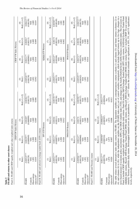
Table 3 reports results using different test assets. Panels A and B focuson different equity portfolios, while Panel C focuses on Treasury securities.The test assets are the CRSP value weighted and equally weighted portfolios(Panel A), equity exchange-traded funds (Panel B), and the CRSP ten-yearconstant maturity Treasury portfolio (Panel C). The equity ETFs include theS&P 500 index ETF (SPY), the NASDAQ 100 ETF (QQQQ), the Russell1000 Index ETF (IWB), and the Russell 2000 Index ETF (IWM). Across allassets, a contemporaneous increase in FEARS is always associated with acontemporaneous decrease of equity returns, and a contemporaneous increaseof Treasury security returns. Moreover, an increase in FEARS today (i.e., k =0)always predicts a return reversal in the coming two days (i.e., k =1 and k =2).The effect of FEARS on equities is typically larger in both initial and futurereturns compared with Treasury securities. A standard-deviation increase in

14

at University of N

otre Dam

e on Novem


Dow

nloaded from


[11:32 28/10/2014 RFS-hhu072.tex] Page: 15 1–34


FEARS corresponds with a contemporaneous decrease of 18 to 19 basis pointsamong equities at k =0 (significant at the 1% level), and a reversal of 14 to 15basis points during the next two days (k =1 and 2, significant at the 1%–5%level). In contrast, a standard-deviation increase in FEARS corresponds witha contemporaneous increase of 4 basis points for Treasury securities at k =0(significant at the 1% level), and a complete reversal over the next two days(significant at the 1% level). Also, because the portfolios include more smallstocks in Panel B (from the S&P 500 index, to the Russell 1000 Index, and thento the Russell 2000 Index) we observe a stronger reversal effect associated withour FEARS index.

Of course, such a short-term reversal can also be caused by a liquidity shockas in Campbell, Grossman and Wang (1993; GSW hereafter). As Baker andStein (2004) point out, as sentiment and liquidity are intertwined, the differencebetween a sentiment-based story as in DSSW and a liquidity-based story as inGSW boils down how we view liquidity shocks and noise traders. Tetlock(2007) even goes so far as to say that “the difference between DSSW andCGW is philosophical rather than economic.” Our results remain interestingeven under the liquidity interpretation, as they suggest high-frequency investorsentiment, as measured by our FEARS, can be a powerful trigger of a liquidityshock.

Overall, Tables 2 and 3 illustrate that our FEARS index is strongly associatedwith contemporaneous returns and predicts future short-term return reversals.

2.2 FEARS and limits to arbitrageAs highlighted in Baker and Wurgler (2006, 2007), there are several additionalchannels that can exacerbate the effect of sentiment investors on asset prices.Perhaps the most important channel is limits to arbitrage (Pontiff 1996, Shleiferand Vishny 1997). Arbitrage capital moves slowly to take advantage of theirrational beliefs of sentiment investors. Motivated by limits to arbitrage, weconsider several additional testing assets in order to explore the effect ofsentiment on asset prices.

The first set of testing assets is the return spread from beta-sorted portfoliosobtained from CRSP. CRSP computes a Scholes-Williams (1977) beta forcommon stocks traded on NYSE and AMEX using daily returns within a yearand then forms decile portfolios. We take these beta-sorted decile portfolios,and compute the return spread between high beta stocks and low beta stocks.

According to Baker, Bradley, and Wurgler (2011), high-beta portfolios areprone to the speculative trading of sentiment investors. Moreover, high-betastocks may be unattractive to arbitrageurs who face institutional constraintssuch as benchmarking. Because these two forces work in the same directionfor high-beta stocks, it is natural to conjecture that investor sentiment mayhave a larger impact among high-beta stocks than among low-beta stocks.Thus, the return spreads between high-beta and low-beta stock portfolios shouldbe negatively correlated with a contemporaneous increase in FEARS, while

15

at University of N

otre Dam

e on Novem


Dow

nloaded from


[11:32 28/10/2014 RFS-hhu072.tex] Page: 16 1–34

The Review of Financial Studies / v 0 n 0 2014Ta

ble

3F

EA

RS

and

retu

rns

toot

her

asse

tcl

asse

s

Pane

lA:F

EA

RS

and

CR

SPeq

ually

wei

ghte

dan

dva

lue-

wei

ghte

din

dex

retu

rns

CR

SPE

WIn

dex

Ret

urns

CR

SPV

WIn

dex

Ret

urns

(1)

(2)

(3)

(4)

(5)

(6)

(7)

(8)

Ret

(t)

Ret

(t+

1)R

et(t

+2)

Ret

[t+

1,t+

2]R

et(t

)R

et(t

+1)

Ret

(t+

2)R

et[t

+1,

t+2]

FEA

RS

–0.0

0519

***

0.00

195*

*0.

0018

5*0.

0038

1***

–0.0

0526

***

0.00

211*

*0.

0020

1*0.

0041

3***

(0.0

0128

)(0

.000

949)

(0.0

0099

9)(0

.001

33)

(0.0

0130

)(0

.000

981)

(0.0

0113

)(0

.001

39)

Con

trol

sY

ES

YE

SY

ES

YE

SY

ES

YE

SY

ES

YE

SO

bser

vatio

ns1,

891

1,89

01,

889

1,88

91,

891

1,89

01,

889

1,88

9A

djus

ted

R2

0.03

50.

005

0.00

50.

006

0.05

20.

018

0.00

90.

019

Pane

lB:F

EA

RS

and

sele

cted

exch

ange

trad

edfu

nds

(ET

Fs)

retu

rns

SPY

ET

FR

etur

nsQ

QQ

QE

TF

Ret

urns

(1)

(2)

(3)

(4)

(5)

(6)

(7)

(8)

Ret

(t)

Ret

(t+

1)R

et(t

+2)

Ret

[t+

1,t+

2]R

et(t

)R

et(t

+1)

Ret

(t+

2)R

et[t

+1,

t+2]

FEA

RS

–0.0

0527

***

0.00

213*

*0.

0016

40.

0037

8***

–0.0

0457

***

0.00

214*

*0.

0017

30.

0038

5***

(0.0

0136

)(0

.000

971)

(0.0

0111

)(0

.001

36)

(0.0

0133

)(0

.001

06)

(0.0

0116

)(0

.001

49)

Con

trol

sY

ES

YE

SY

ES

YE

SY

ES

YE

SY

ES

YE

SO

bser

vatio

ns1,

891

1,89

01,

889

1,88

91,

885

1,88

31,

882

1,88

1A

djus

ted

R2

0.05

80.

026

0.01

20.

026

0.03

00.

009

0.00

20.

008

IWB

ET

FR

etur

nsIW

ME

TF

Ret

urns

(1)

(2)

(3)

(4)

(5)

(6)

(7)

(8)

Ret

(t)

Ret

(t+

1)R

et(t

+2)

Ret

[t+

1,t+

2]R

et(t

)R

et(t

+1)

Ret

(t+

2)R

et[t

+1,

t+2]

FEA

RS

–0.0

0506

***

0.00

214*

*0.

0017

40.

0039

0***

–0.0

0529

***

0.00

272*

*0.

0019

60.

0047

2***

(0.0

0128

)(0

.000

960)

(0.0

0111

)(0

.001

37)

(0.0

0162

)(0

.001

24)

(0.0

0145

)(0

.001

78)

Con

trol

sY

ES

YE

SY

ES

YE

SY

ES

YE

SY

ES

YE

SO

bser

vatio

ns1,

891

1,89

01,

889

1,88

91,

891

1,89

01,

889

1,88

9A

djus

ted

R2

0.05

20.

019

0.00

90.

019

0.04

10.

014

0.00

50.

015

Pane

lC:F

EA

RS

and

Tre

asur

yre

turn

s

(1)

(2)

(3)

(4)

Ret

(t)

Ret

(t+

1)R

et(t

+2)

Ret

[t+

1,t+

2]

FEA

RS

0.00

112*

**–0

.000

540*

–0.0

0062

4**

–0.0

0117

***

(0.0

0037

8)(0

.000

324)

(0.0

0030

7)(0

.000

426)

Con

stan

tY

esY

esY

esY

esO

bser

vatio

ns1,

876

1,87

51,

874

1,87

4A

djus

ted

R2

0.02

00.

007

0.00

80.

013

Thi

sta

ble

rela

tes

seve

ral

alte

rnat

ive

inde

xda

ilyre

turn

sto

FEA

RS.

The

depe

nden

tva

riab

les

are

cont

empo

rane

ous

retu

rns

(col

umn

(1)

and

colu

mn

(5))

and

futu

rere

turn

s(c

olum

ns(2

)to

(4),

and

colu

mns

(6)

to(8

)),

whi

leth

ein

depe

nden

tva

riab

les

are

the

FEA

RS

inde

xan

da

set

ofco

ntro

lva

riab

les

(unr

epor

ted)

,w

hich

incl

ude

lagg

edre

turn

sup

tofiv

ela

gs,

chan

ges

ina

new

s-ba

sed

mea

sure

ofec

onom

icpo

licy

unce

rtai

nty

(EPU

),th

eC

BO

Evo

latil

ityin

dex

(VIX

),an

dch

ange

sin

the

Aru

oba-

Die

bold

-Sco

tti(A

DS)

busi

ness

cond

ition

sin

dex.

The

test

asse

tsin

Pane

lAin

clud

eC

RSP

equa

llyw

eigh

ted

and

valu

e-w

eigh

ted

port

folio

daily

retu

rns.

Pane

lB

incl

udes

S&P

Exc

hang

eT

rade

dFu

nd(S

PY)

daily

retu

rns,

NA

SD

AQ

Exc

hang

eT

rade

dFu

nd(Q

QQ

Q)

daily

retu

rns,

Rus

sell

1000

Exc

hang

eT

rade

dFu

nd(I

WB

)da

ilyre

turn

s,an

dR

usse

ll20

00E

xcha

nge

Tra

ded

Fund

(IW

M)

daily

retu

rns.

Pane

lC

incl

udes

CR

SP10

-yea

rco

nsta

ntm

atur

ityT

reas

ury

port

folio

daily

retu

rns.

Boo

tstr

appe

dst

anda

rder

rors

are

inpa

rent

hese

s.*,

**,a

nd**

*de

note

the

coef

ficie

ntes

timat

esar

esi

gnifi

cant

at10

%,5

%,a

nd1%

sign

ifica

nce

leve

ls,r

espe

ctiv

ely.

16

at University of N

otre Dam

e on Novem


Dow

nloaded from


[11:32 28/10/2014 RFS-hhu072.tex] Page: 17 1–34


future return spreads should be positively correlated with current increases inFEARS. Motivated byWurgler and Zhuravskaya (2002), we also use total returnvolatility as a proxy for limits to arbitrage and examine the aforementionedreversal pattern for a portfolio of stocks with high volatility versus a portfolioof stocks with low volatility. The volatility-sorted portfolios are also obtainedfrom CRSP. Using daily stock returns within a calendar year, CRSP computesthe total return volatility of common stocks traded on NYSE and AMEX, andcreates decile portfolios based on total return volatility.

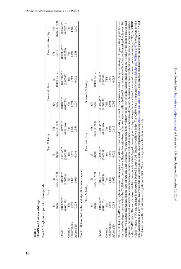
Panel A from Table 4 confirms the hypothesis. As shown in Panel A, columns1 and 2, sentiment has a more negative contemporaneous relationship withhigh-beta stocks. For example, a one-standard-deviation increase in FEARSis associated with a 22-basis-points decrease in the return spread between thehigh-beta and low-beta stock portfolio (statistically significant at the 1% level).Again, FEARS also predicts future return reversal effects. By k =2 , the effectis almost completely reversed. Likewise in columns 3 and 4, we find FEARSto have stronger impact on high-volatility stocks than low-volatility stocks onday t , while the impact is almost completely reversed by the end of the secondday (k =2).

Certain assets are also prone to “downside” risk. As Ang, Chen, and Xing(2006) observe, “downside” risk is not well captured by conventional beta fromthe capital asset pricing model (CAPM). If downside risk is particularly largewhen investor sentiment is high, we anticipate that a portfolio of stocks withhigh downside risk should underperform a portfolio of stocks with relativelylow downside risk because downside risk limits arbitrageurs from correctingmispricing. Following Ang, Chen, and Xing (2006), we consider two measuresof “downside risk.” The first measure is “downside beta,” which was firstintroduced by Bawa and Lindenberg (1977). Specifically, at the end of eachmonth, we estimate the “downside beta” (i.e., β−

i ) for individual stocks asfollows,

β−i =

cov(ri,rm|rm <μm)

var (rm|rm <μm), (4)

using the past year of daily returns.The second measure of downside risk is “downside sigma” (i.e., σ−

i ), whichis defined as follows:

σ−i =

√var (ri |rm <μm), (5)

and it is also estimated using the past year of daily returns on a monthly basis.Analogous to the beta-sorted or the total return volatility-sorted portfolios

constructed by CRSP, we create decile portfolios on the basis of the stock-levelestimates of “downside beta” or “downside sigma” for individual stocks. Wetrack daily portfolio returns over the next month, and rebalance the portfolio atthe end of the next month. The return spreads between the returns of the high“downside beta” and low “downside beta” stock portfolios are the test assets incolumns 5 and 6 of PanelA. Similarly, columns 7 and 8 relate FEARS and return

17

at University of N

otre Dam

e on Novem


Dow

nloaded from


[11:32 28/10/2014 RFS-hhu072.tex] Page: 18 1–34


Tabl

e4

FE

AR

San

dlim

its

toar

bitr

age

Pane

lA:S

ingl

e-so

rted

port

folio

retu

rnsp

read

s

Bet

aTo

talV

olat

ility

Dow

nsid

eB

eta

Dow

nsid

eV

olat

ility

(1)

(2)

(3)

(4)

(5)

(6)

(7)

(8)

Ret

(t)

Ret

[t+

1,t+

2]R

et(t

)R

et[t

+1,

t+2]

Ret

(t)

Ret

[t+

1,t+

2]R

et(t

)R

et[t

+1,

t+2]

FEA

RS

–0.0

0620

***

0.00

641*

**–0

.003

6***

0.00

397*

**–0

.010

6***

0.00

716*

**–0

.009

04**

*0.

0062

3**

(0.0

0199

)(0

.002

26)

(0.0

0131

)(0

.001

46)

(0.0

0233

)(0

.002

43)

(0.0

0228

)(0

.002

51)

Con

trol

sY

esY

esY

esY

esY

esY

esY

esY

esO

bser

vatio

ns1,

891

1,88

91,

891

1,88

91,

891

1,88

91,

891

1,88

9A

djus

ted

R2

0.02

30.

010

0.04

60.

059

0.03

90.

012

0.03

80.

017

Pane

lB:B

eta-

neut

rald

oubl

e-so

rted

port

folio

retu

rnsp

read

s

Tota

lVol

atili

tyD

owns

ide

Bet

aD

owns

ide

Vol

atili

ty

(1)

(2)

(3)

(4)

(5)

(6)

Ret

(t)

Ret

[t+

1,t+

2]R

et(t

)R

et[t

+1,

t+2]

Ret

(t)

Ret

[t+

1,t+

2]

FEA

RS

–0.0

0414

***

0.00

320*

**–0

.006

14**

*0.

0047

4***

–0.0

0374

***

0.00

234*

*(0

.001

03)

(0.0

0119

)(0

.001

51)

(0.0

0148

)(0

.000

837)

(0.0

0102

)C

ontr

ols

Yes

Yes

Yes

Yes

YE

SY

ES

Obs

erva

tions

1,89

11,

891

1,89

11,

891

1,89

11,

891

Adj

uste

dR

20.

088

0.05

50.

052

0.01

30.

092

0.06

5

Thi

sta

ble

links

FEA

RS

toda

ilyhi

gh-m

inus

-low

retu

rnsp

read

son

port

folio

sco

nstr

ucte

dby

sort

ing

onst

ock

char

acte

rist

ics

rela

ted

tolim

itsto

arbi

trag

e.In

pane

l,th

ese

port

folio

sar

eco

nstr

ucte

dby

sing

leso

rts

onei

ther

the

CA

PMbe

ta,t

heto

talv

olat

ility

,the

dow

nsid

ebe

ta,o

rth

edo

wns

ide

vola

tility

.In

Pane

lB,w

ere

mov

eth

eef

fect

from

the

beta

usin

gdo

uble

sort

s.Fo

rex

ampl

e,w

eco

nduc

tind

epen

dent

doub

leso

rts

onbe

taan

dto

talv

olat

ility

.We

then

com

pute

high

-vol

atili

ty-m

inus

-low

-vol

atili

tyre

turn

spre

ads

usin

gon

lyst

ocks

with

sim

ilar

beta

s.In

each

regr

essi

on,t

hede

pend

ent

vari

able

sar

eco

ntem

pora

neou

sre

turn

s(c

olum

nw

ithod

dnu

mbe

rs)

and

next

-tw

o-da

yre

turn

s(c

olum

nsw

ithev

ennu

mbe

rs)

whi

leth

em

ain

inde

pend

ent

vari

able

isth

eFE

AR

Sin

dex.

The

set

ofco

ntro

lva

riab

les

(unr

epor

ted)

incl

ude

lagg

edre

turn

sup

tofiv

ela

gs,

chan

ges

ina

new

-bas

edm

easu

reof

econ

omic

polic

yun

cert

aint

y(E

PU),

the

CB

OE

vola

tility

inde

x(V

IX),

and

chan

ges

inth

eA

ruob

a-D

iebo

ld-S

cotti

(AD

S)bu

sine

ssco

nditi

ons

inde

x.T

heC

APM

beta

isco

mpu

ted

follo

win

gSc

hole

san

dW

illia

ms

(197

7)to

acco

untf

orth

eno

n-sy

nchr

onic

ityin

daily

retu

rns.

Dow

nsid

ebe

taan

ddo

wns

ide

vola

tility

are

com

pute

dfo

llow

ing

Ang

,Che

n,an

dX

ing

(200

6).B

oots

trap

ped

stan

dard

erro

rsar

ein

pare

nthe

ses.

*,**

and

***

deno

teth

eco

effic

ient

estim

ates

are

sign

ifica

ntat

10%

,5%

and

1%si

gnifi

canc

ele

vels

,res

pect

ivel

y.

18

at University of N

otre Dam

e on Novem


Dow

nloaded from


[11:32 28/10/2014 RFS-hhu072.tex] Page: 19 1–34


spreads between the high “downside sigma” and low “downside sigma” stockportfolios. The effect of sentiment on these return spreads is large. For instance,a one-standard-deviation increase in FEARS is associated with a decrease of37 basis points in the return spreads between the high downside beta and lowdownside beta stock portfolio (statistically significant at the 1% level). Again,FEARS also predicts future return reversals. By k =2 , the reversal of the returnspreads associated with FEARS is about 25 basis points. Thus, sentiment hasa stronger effect on high downside beta stocks than low downside beta stockson day t , while the impact almost completely reverses back by the end of thesecond day (k =2) after event day t , or k =0 . Similar results are obtained usingthe high-minus-low-downside-volatility portfolio return spreads.

We have shown earlier that FEARS predict a reversal in market return.Because stocks that are difficult to arbitrage tend to have higher betas, it isperhaps not surprising that FEARS predicts a stronger reversal among thesestocks. In other words, the cross-sectional results in Panel A of Table 4 couldbe driven by a mechanical “beta effect.” To examine whether “beta effect” isdriving the results shown in Panel A, we construct a series of double-sortedportfolios to account for potential differences in betas across testing assets.Specifically, at the end of each month, we first compute the Scholes-Williams(1977) beta for each stock, using the past twelve-month daily returns. To ensurethat our sample is comparable to various decile-sorted portfolios constructedby CRSP and further alleviate liquidity concerns, we restrict our sample tostocks from NYSE and AMEX. We sort these stocks into quintile portfolios.Within each quintile portfolio, we further sort stocks into another set of quintileportfolios based on total volatility, downside beta, or downside volatility (asestimated before). From each beta-sorted quintile portfolio, we compute thereturn spreads between the high and low total volatility, downside beta, ordownside volatility portfolios, and take the average across the beta-sortedquintiles. These double-sorted portfolios generate return spreads with varyingdegrees of limits to arbitrage, but are beta-neutral.

Panel B of Table 4 reports our results. After removing the “beta effect,”FEARS still significantly predicts reversals on the three beta-neutral returnspreads due to differences in total volatility (columns 1 and 2), downside beta(columns 3 and 4), or downside volatility (columns 5 and 6), although themagnitudes of the reversals are in general smaller than those reported in PanelA. For example, a one-standard-deviation increase in FEARS is associatedwith a 22-basis-points decrease in the return spreads between the high andlow downside-beta stock portfolio (statistically significant at the 1% level). Byk =2 , the reversal of the return spreads associated with FEARS is about 17 basispoints (statistically significant at the 1% level)—or about 77.3% (=17/22) ofreversal of initial return spreads.

Overall, this evidence provides additional support for the sentiment modelof Baker and Wurgler (2006, 2007), which highlights the interaction betweenspeculative trading and limits to arbitrage. It also provides cross-sectional

19

at University of N

otre Dam

e on Novem


Dow

nloaded from


[11:32 28/10/2014 RFS-hhu072.tex] Page: 20 1–34


evidence for sentiment-induced mispricing. Among the set of stocks for whichsentiment is most likely to operate, we find the strongest evidence of temporarydeviation from fundamentals.

2.3 Robustness checksConstruction of our FEARS index required several choices, and in this sectionwe examine the robustness of our results to those choices and the inclusion ofadditional control variables.

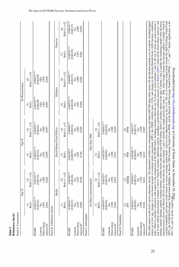
For example, we use the thirty search terms whose �ASV I s are mostnegatively correlated with the market return in our backward rolling window.Averaging FEARS across many search terms allows us to capture their commonvariation and, at the same time, alleviate idiosyncratic noise. In Panel A ofTable 5, we construct alternative FEARS indices by averaging the top twenty-five search terms and top thirty-five search terms. Comparing the results inTable 5, Panel A, with those in Table 2, we find that the alternative FEARSindices produce very similar results. Moreover, to alleviate the effect fromextreme outliers in the construction of the FEARS index, we also winsorizedthe series for each search term at the 5% level (2.5% in each tail). A potentialconcern about applying winsorization in the context of predictive regressionsis that it could introduce a forward-looking bias. To address this concern, thefinal columns of Panel A report the results of using FEARS indices constructedwithout winsorization. The results are again very similar to those in Panel A ofTable 2, if not slightly stronger.

In the main test specifications, we have been using a news-based measureof economic policy uncertainty (EPU ), the CBOE volatility index (V IX),and Aruoba-Diebold-Scotti (ADS) business conditions index as our controlsfor economic uncertainty, investor sentiment, and macroeconomic conditions.There are also news-based investor sentiment measures. For example, Tetlock(2007) proposes a news-based sentiment measure using the fraction of negativewords in the Wall Street Journal “Abreast of the Market” column. The news-based investor sentiment measure is available to us through 2010, and this iswhy we do not include it in our benchmark regressions. Nevertheless, the firsttwo columns of Table 5, Panel B, shows that in this shorter sample our resultsare robustness to the inclusion of it as an additional control.

Another potential concern regarding our results is that FEARS could simplyproxy for extreme market returns, which are more likely to revert in the future.Although we have included the market return and additional lags as controlvariables in our regressions, one may still be concerned that the FEARS indexsimply captures a nonlinear effect from large market returns. To address thisconcern, we include decile dummies for the market return in our regressions incolumns 3 and 4 of Panel B. Little changes after the inclusion of these deciledummies.

The next two columns consider the effect of holidays on search and returns.Because search patterns may systematically change around holidays and there

20

at University of N

otre Dam

e on Novem


Dow

nloaded from


[11:32 28/10/2014 RFS-hhu072.tex] Page: 21 1–34

The Sum of All FEARS Investor Sentiment and Asset PricesTa

ble

5R

obus

tnes

sch

ecks

Pane

lA:C

onst

ruct

ion

Top

25To

p35

No

Win

sori

zatio

n

(1)

(2)

(3)

(4)

(5)

(6)

Ret

(t)

Ret

[t+

1,t+

2]R

et(t

)R

et[t

+1,

t+2]

Ret

(t)

Ret

[t+

1,t+

2]

FEA

RS

–0.0

0513

***

0.00

374*

**–0

.005

23**

*0.

0042

8***

–0.0

0578

***

0.00

437*

**(0

.001

24)

(0.0

0132

)(0

.001

33)

(0.0

0141

)(0

.001

46)

(0.0

0149

)C

ontr

ols

Yes

Yes

Yes

Yes

YE

SY

ES

Obs

erva

tions

1,89

11,

889

1,89

11,

889

1,86

11,

859

Adj

uste

dR

20.

061

0.02

60.

059

0.02

70.

067

0.02

8

Pane

lB:A

dditi

onal

cont

rols

Med

iaD

ecile

Ret

urn

Fixe

dE

ffec

tsH

olid

ays

Tur

nove

r

(1)

(2)

(3)

(4)

(5)

(6)

(7)

(8)

Ret

(t)

Ret

[t+

1,t+

2]R

et(t

)R

et[t

+1,

t+2]

Ret

(t)

Ret

[t+

1,t+

2]R

et(t

)R

et[t

+1,

t+2]

FEA

RS

–0.0

0564

***

0.00

448*

**–0

.001

90**

0.00

400*

**–0

.005

33**

*0.

0040

9***

–0.0

0525

***

0.00

419*

**(0

.001

33)

(0.0

0148

)(0

.000

797)

(0.0

0134

)(0

.001

30)

(0.0

0137

)(0

.001

29)

(0.0

0137

)C

ontr

ols

Yes

Yes

Yes

Yes

Yes

Yes

Yes

Yes

Obs

erva

tions

1,63

91,

639

1,89

11,

889

1,89

11,

889

1,89

11,

889

Adj

uste

dR

20.

068

0.03

40.

794

0.02

90.

060

0.02

60.

061

0.02

9

Pane

lC:S

ubsa

mpl

es

No

Mac

roA

nnou

ncem

ents

Aft

erJu

ne20

06

(1)

(2)

(3)

(4)

Ret

(t)

Ret

[t+

1,t+

2]R

et(t

)R

et[t

+1,

t+2]

FEA

RS

–0.0

0539

***

0.00

325*

*–0

.007

59**

*0.

0056

3***

(0.0

0144

)(0

.001

39)

(0.0

0202

)(0

.001

92)

Con

trol

sY

esY

esY

esY

esO

bser

vatio

ns1,

586

1,58

41,

408

1,40

6A

djus

ted

R2

0.05

80.

032

0.07

30.

029

Pane

lD:T

rada

bilit

y

(1)

(2)

(3)

(4)

SPY

QQ

QQ

IWB

IWM

FEA

RS

0.00

262*

**0.

0026

5**

0.00

268*

**0.

0027

3**

(0.0

0101

)(0

.001

15)

(0.0

0101

)(0

.001

33)

Con

trol

sY

esY

esY

esY

esO

bser

vatio

ns1,

508

1,50

21,

508

1,50

8A

djus

ted

R2

0.01

60.

011

0.01

30.

007

Thi

sta

ble

repo

rts

resu

ltsfr

omva

riou

sro

bust

ness

chec

ks.T

hede

pend

entv

aria

bles

are

cont

empo

rane

ous

and

futu

reS&

P50

0in

dex

daily

retu

rns

All

spec

ifica

tion

incl

ude

ase

tof

cont

rols

,inc

ludi

ngla

gged

retu

rns

upto

five

lags

,cha

nges

ina

new

-bas

edm

easu

reof

econ

omic

polic

yun

cert

aint

y(E

PU),

the

CB

OE

vola

tility

inde

x(V

IX),

and

chan

ges

inth

eA

ruob

a-D

iebo

ld-S

cotti

(AD

S)bu

sine

ssco

nditi

ons

inde

x.Pa

nelA

cons

ider

sro

bust

ness

with

resp

ect

toth

eco

nstr

uctio

nof

the

FEA

RS

inde

x,in

clud

ing

estim

ates

whe

nth

eto

p25

term

sar

eus

ed(c

olum

ns1

and

2),t

heto

p35

term

sar

eus

ed(c

olum

ns3

and

4)an

dw

ithou

tw

inso

riza

tion

(col

umns

5an

d6)

.Pa

nel

Bco

nsid

ers

addi

tiona

lco

ntro

ls,

incl

udin

ga

med

ia-b

ased

sent

imen

tm

easu

reas

inTe

tlock

(200

7),

retu

rnde

cile

fixed

effe

cts,

turn

over

,an

dho

liday

cont

rols

.Hol

iday

cont

rols

cons

titut

edu

mm

yva

riab

les

befo

rean

daf

ter

each

NY

SEho

liday

.Pan

elC

cons

ider

ssu

bset

sof

the

data

.Col

umns

1an

d2

cons

ider

the

rem

aini

ngsa

mpl

ew

hen

allm

acro

anno

unce

men

ts(S

avor

and

Wils

on(2

012)

)ha

vebe

enth

row

nou

t,an

dco

lum

ns3

and

4co

nsid

erth

esa

mpl

epe

riod

afte

rJu

ne1,

2006

,w

hen

Goo

gle

Tre

nds

data

beca

me

publ

icly

avai

labl

e.Pa

nel

Dco

nsid

ers

trad

abili

tyan

dre

port

sre

sults

base

don

vari

ous

exch

ange

trad

edfu

nds’

open

-to-

clos

ead

just

ed-r

etur

nson

day

(t+

2).T

hese

tof

exch

ange

trad

edfu

nds

incl

ude

the

S&P

Exc

hang

eT

rade

dFu

nd(S

PY),

the

NA

SDA

QE

xcha

nge

Tra

ded

Fund

(QQ

QQ

),th

eR

usse

ll10

00E

xcha

nge

Tra

ded

Fund

(IW

B),

and

the

Rus

sell

2000

Exc

hang

eT

rade

dFu

nd(I

WM

).*,

**,a

nd**

*de

note

sign

ifica

nce

atth

e10

%,5

%,a

nd1%

leve

ls,r

espe

ctiv

ely.

21

at University of N

otre Dam

e on Novem


Dow

nloaded from


[11:32 28/10/2014 RFS-hhu072.tex] Page: 22 1–34


is some evidence of holiday-related return phenomenon (see Ariel 1990, forexample), columns 5 and 6 of Panel B remove holiday effects by includingadditional dummy variables for the trading day before and the trading day afterpublic holidays in our sample. Little changes after the inclusion of holidaycontrols.

Although we interpret the spike-reversal pattern herein as evidence ofsentiment, such a pattern is potentially consistent with a liquidity shockfollowing an economic event. The economic event could trigger spikes inboth search volume and liquidity trades, pushing prices temporarily away fromfundamentals ( 1993). This would also generate the predictable spike-reversalpattern we find. We address this alternative in a few ways. First, we includethe turnover of the S&P 500 index as a control variable in columns 7 and 8of Panel B.15 Controlling for liquidity in this way does little to change theresults. Second, we obtain macro announcement dates as in Savor and Wilson(2013) and remove all observations with macro announcements. The idea isthat although periodical macro announcements may affect investor sentiment,they may also induce portfolio rebalancing and generate liquidity shocks. InTable 5, Panel C, we find the same spike-reversal pattern among observationswithout macro announcements. Third, recall that we find larger effects amonghard-to-arbitrage stocks in Section 2.2. A liquidity hypothesis is unlikely togenerate the same cross-sectional pattern in stocks.

Finally, we have been using the FEARS index on day t to “predict” assetreturns on days t +1 and t +2 as we try to understand the economic impactof investor sentiment on contemporaneous and future prices. Because Googlereleases its SVI data with a one-day delay, these predictive regressions cannot berun in real time. For example, the SVI for a search term on Wednesday, January23, will typically be released sometime during the evening of Thursday, January24. Moreover, Google only made this data publicly available in June 2006.

Panels C and D demonstrate the robustness of our reversal results whenthe predictive regressions are implemented when data are available. The finalcolumns of Panel C consider the subset of observations beginning in June 2006when search data were available and finds little change in the main result.Panel D considers the predictability of day t +2 open-to-close returns with dayt search volume. Continuing with the earlier example, it means that we useour FEARS index on Wednesday, January 23 (observable by the evening ofThursday, January 24) to predict the open-to-close returns on Friday, January25. In other words, the predictive variables are strictly observable before theasset return can be computed. Because open prices are needed for this analysis,we focus our attention on ETFs. The results in Panel D confirm the strong andsignificant reversals across all four ETFs. The regression coefficients are onlyslightly smaller compared with those in Table 3, Panel B, reflecting the fact

15 In untabulated results we also find that controlling for signed turnover — that is, the interaction of turnover onday t with the return on day t, does not change the reversal results on days t+1 and t+2.

22

at University of N

otre Dam

e on Novem


Dow

nloaded from


[11:32 28/10/2014 RFS-hhu072.tex] Page: 23 1–34


that we are using open-to-close returns rather than the standard close-to-closereturns.

3. FEARS and Volatility

A long strand of literature starting from Black (1986) suggests that investorsentiment and the resulting noise trading can affect both the level and thevolatility of asset prices. If uninformed noise traders base their trading decisionson sentiment, then extreme sentiment changes will temporarily lead to morenoise trading, greater mispricing, and excessive volatility. To our knowledge, noprior work has examined the relation between sentiment measures and market-level volatility at a high frequency.16 In this section we examine the relationshipbetween FEARS and various stock market return volatility measures. Theresults are reported in Table 6.

We start by examining two direct measures of stock market volatility. The firstmeasure is realized volatility (RV), developed byAndersen, Bollerslev, Dieboldand Ebens (2001) and Andersen, Bollerslev, Diebold, and Labys (2003). Weimplement the realized volatility estimation procedure by closely followingAndersen, Bollerslev, Diebold and Ebens (2001). Since intraday transactiondata are needed to calculate daily realized volatilities, we focus our attentionon the SPDR S&P 500 ETF (NYSEARCA: SPY) as a close proxy for the stockmarket index. The SPYETF is extremely liquid. For instance, the bid-ask spreadis almost always one cent, the minimum tick size. Similar to Antweiler andFrank (2004), we choose fifteen-minute periods when we sample the intradayreturns. rt,d denotes the intraday return for SPY during the d -th period on dayt . SPY’s (annualized) realized volatility on day t is given by

rυt =250N∑

d=1

r2t,d . (6)

We then compute daily log realized volatility, rv , and remove potentialseasonal effects by regressing it on day-of-the-week and month-of-the-year dummies. We focus on the residuals, or the seasonal-adjusted logRV time series (adj_rv). Because volatility is persistent and long-lived(Engel and Patton (2001); Andersen, Bollerslev, Diebold and Ebens 2001;Andersen, Bollerslev, Diebold, and Labys 2003), we also model the long-rangedependence through the fractional integrated autoregressive moving averagemodel, ARFIMA(1,d,1) :

(1−L)d(

adj_rvt −β1FEARSt −∑m

βmControlmi,t

)=(1−L)εt (7)

16 Using Yahoo! message board activities as a proxy for noise trading, Antweiler and Frank (2004) and Koski,Rice, and Tarhouni (2008) confirm the positive relation between noise trading and future volatility at the dailyfrequency for a small set of individual stocks.

23

at University of N

otre Dam

e on Novem


Dow

nloaded from


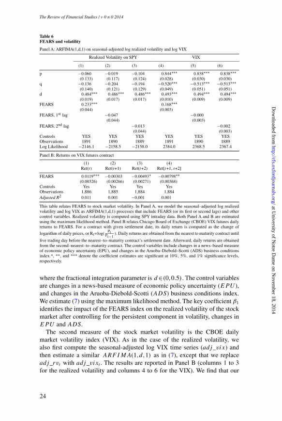
[11:32 28/10/2014 RFS-hhu072.tex] Page: 24 1–34


Table 6FEARS and volatility

Panel A: ARFIMA(1,d,1) on seasonal-adjusted log realized volatility and log VIX

Realized Volatility on SPY VIX

(1) (2) (3) (4) (5) (6)

p −0.060 −0.019 −0.104 0.844∗∗∗ 0.838∗∗∗ 0.838∗∗∗(0.133) (0.117) (0.124) (0.028) (0.030) (0.030)

q −0.136 −0.204 −0.194 −0.520∗∗∗ −0.513∗∗∗ −0.513∗∗∗(0.140) (0.121) (0.129) (0.049) (0.051) (0.051)

d 0.484∗∗∗ 0.486∗∗∗ 0.486∗∗∗ 0.493∗∗∗ 0.494∗∗∗ 0.494∗∗∗(0.019) (0.017) (0.017) (0.010) (0.009) (0.009)

FEARS 0.233∗∗∗ 0.168∗∗∗(0.044) (0.003)

FEARS, 1st lag −0.047 −0.000(0.044) (0.003)

FEARS, 2nd lag −0.013 −0.002(0.044) (0.003)

Controls YES YES YES YES YES YESObservations 1891 1890 1889 1891 1890 1889Log Likelihood −2146.1 −2158.5 −2158.0 2384.0 2368.5 2367.4

Panel B: Returns on VIX futures contract

(1) (2) (3) (4)Ret(t) Ret(t+1) Ret(t+2) Ret[t+1, t+2]

FEARS 0.0119∗∗∗ −0.00303 −0.00493∗ −0.00798∗∗(0.00326) (0.00266) (0.00271) (0.00368)

Controls Yes Yes Yes YesObservations 1,886 1,885 1,884 1,884Adjusted R2 0.011 0.001 −0.001 0.001

This table relates FEARS to stock market volatility. In Panel A, we model the seasonal–adjusted log realizedvolatility and log VIX as ARFIMA(1,d,1) processes that include FEARS (or its first or second lags) and othercontrol variables. Realized volatility is computed using SPY intraday data. Both Panel A and B are estimatedusing the maximum likelihood method. Panel B relates Chicago Board of Exchange (CBOE) VIX futures dailyreturns to FEARS. For a contract with given settlement date, its daily return is computed as the change of

logarithm of daily prices, or Rt= log( PtPt−1

). Daily returns are obtained from the nearest to maturity contract until

five trading day before the nearest–to–maturity contract’s settlement date. Afterward, daily returns are obtainedfrom the second–nearest–to–maturity contract. The control variables include changes in a news–based measureof economic policy uncertainty (EPU), and changes in the Aruoba–Diebold–Scotti (ADS) business conditionsindex.*, **, and *** denote the coefficient estimates are significant at 10%, 5%, and 1% significance levels,respectively.

where the fractional integration parameter is d ∈ (0,0.5) . The control variablesare changes in a news-based measure of economic policy uncertainty (EPU ),and changes in the Aruoba-Diebold-Scotti (ADS) business conditions index.We estimate (7) using the maximum likelihood method. The key coefficient β1

identifies the impact of the FEARS index on the realized volatility of the stockmarket after controlling for the persistent component in volatility, changes inEPU and ADS.

The second measure of the stock market volatility is the CBOE dailymarket volatility index (VIX). As in the case of the realized volatility, wealso first compute the seasonal-adjusted log VIX time series (adj_vix) andthen estimate a similar ARFIMA(1,d,1) as in (7), except that we replaceadj_rvt with adj_vixt . The results are reported in Panel B (columns 1 to 3for the realized volatility and columns 4 to 6 for the VIX). We find that our

24

at University of N

otre Dam

e on Novem


Dow

nloaded from


[11:32 28/10/2014 RFS-hhu072.tex] Page: 25 1–34


FEARS index is positively and significantly related to the market volatilitymeasures only contemporaneously (see columns 1 and 4). Controlling for thepersistent component in volatility, neither realized volatility nor VIX loadssignificantly on lagged FEARS index. These results again suggest that ourFEARS index has only a transitory impact on the level of stock marketvolatility.

Second, parallel to our analysis in the previous sections, we also examinedaily returns to a tradable asset based on volatility, the CBOE VIX futurescontract. Working with the return series has the benefit of circumventingpotential econometric issues associated with the VIX and RV time series andproviding a clear interpretation of asset returns. For a contract with a givensettlement date, its daily return is computed as the change of log daily prices.17

We then use our FEARS index to predict these daily VIX futures returns usingthe same regression specifications in Equation (3). The results are reported inPanel C.

Panel C confirms the strong contemporaneous correlation between FEARSand volatility. For example, a one standard deviation increase in FEARScorresponds with a contemporaneous 42-basis-points increase in VIX futuresreturn. In the next two trading days, we again find a reversal pattern. Bythe end of the second trading day, we observe a total reversal of 28 basispoints.

Thus far analyzing both the levels and changes in stock market volatility, ourresults paint a consistent picture: an increase in our FEARS index coincideswith an increase in market volatility that is temporary. To the extent that aspike in our FEARS index coincides with more noise trading, our evidenceprovides further support for the DSSW model, where noise trading leads toexcessive volatility temporarily. The DSSW model also predicts a positiverelation between the volatility of sentiment and the volatility of the assetprice (see equation 11 in DSSW). The intuition is simple: if sentimentcontributes to a temporary price deviation from fundamental value, then themore volatile sentiment is, the higher the excessive price volatility shouldbe. While our focus is on the level of investor sentiment as measured by ourFEARS index, we also try to analyze the joint volatility dynamics between ourFEARS index and market returns. Specifically, we model daily stock marketexcess return and our FEARS index jointly using a multivariate GARCHwith dynamic conditional correlation (see Engle (2000)). Unreported resultsconfirm a significant positive correlation of 7.17% (p-value of 0.002) betweenthe conditional variance of the stock market return and that of the FEARSindex.

17 Daily returns are calculated using the contract closest to maturity except when this contract is less than five daysaway. When the closest to maturity contract is less than five days away, daily returns are calculated from thesecond closest to maturity contract.

25

at University of N

otre Dam

e on Novem


Dow

nloaded from


[11:32 28/10/2014 RFS-hhu072.tex] Page: 26 1–34


4. FEARS and Fund Flows

Noise traders affect asset prices via trading. To directly examine the sentimenteffects of noise traders, we examine daily mutual fund flows in our last setof tests. Because individual investors hold about 90% of total mutual fundassets, and they are more likely to be sentiment traders, daily flows to mutualfund groups likely aggregate noise trading at the asset-class level (Brown,Goetzmann, Hiraki, Shiraishi, and Watanabe 2002 2002). Daily mutual fundflow data are obtained from TrimTabs for two groups of mutual funds thatspecialize in equity (Equity) and intermediate treasury bonds (MTB).

Bollerslev and Jubinski (1999) and Fleming and Kirby (2006) provideevidence that an individual stock’s daily trading volume series exhibits long-runtemporary dependencies, which can be modeled using a fractionally integratedprocess. Similar to observations made on the volume of individual stocks, wealso find very strong persistence and long-memory components in daily fundflows. For this reason, we first demean each of the daily fund flow series, andapply the ARFIMA(p,d,q) models to extract daily fund flow innovations.Our diagnostics indicate that the ARFMA(1,d,1) model fits the underlyingdaily fund flows well. The integration parameter values are in the neighborhoodof 0.40 and p-value less than 0.1%. In addition, the moving average (MA) aswell as the autoregressive (AR) terms are all statistically significant at the 1%level or better.

There is one data issue worth pointing out. TrimTabs mutual fund flow iscalculated using both publicly observable net asset value (NAV) and privatelyreported total asset value (NTA). Despite the obvious accuracy of NAV, theNTA information might be reported with a delay of one day for some funds.Both Edelen and Warner (2002) as well as Greene and Hodges (2002) documentthis issue, and analyze it in detail. Because of this potential one-day reportingdelay, we note that TrimTabs flow in day t +1 may actually contain flow in dayt (see also Yuan (2008)). We run regressions of contemporaneous fund flowsand fund flows one to four days ahead. In particular, we run the followingregression:

f lowi,t+k =β0 +β1FEARSt +∑m

γmControlmi,t +ui,t+k (8)

where fund class i includes bond and equity funds. Controlvariables(Controlmi,t ) include as usual V IX, �EPU , �ADS, and fivelags of market returns. The results of these regressions are reported in Table 7.

We find that our FEARS index has significant incremental predictive powerfor future daily fund flow innovations of both equity and bond funds. In theequity flow regressions, the coefficient on FEARS is negative on each day weconsider (t =0,1,2,3, and 4) and is statistically significant for days t +1 (p-value< 10%), t +2 (p-value < 5%) and t +3 (p-value < 10%). The results suggest thatinvestors start to withdraw from equity mutual funds the day during the spikein FEARS (recall that the outflow on t +1 may actually contain outflow in day t

26

at University of N

otre Dam

e on Novem


Dow

nloaded from


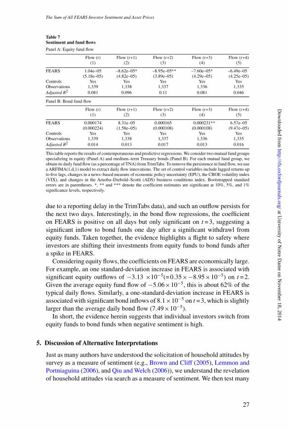
[11:32 28/10/2014 RFS-hhu072.tex] Page: 27 1–34


Table 7Sentiment and fund flows

Panel A: Equity fund flow

Flow (t) Flow (t+1) Flow (t+2) Flow (t+3) Flow (t+4)(1) (2) (3) (4) (5)

FEARS 1.04e–05 –8.62e–05* –8.95e–05** –7.60e–05* –6.49e–05(5.18e–05) (4.82e–05) (3.89e–05) (4.29e–05) (4.25e–05)

Controls Yes Yes Yes Yes YesObservations 1,339 1,338 1,337 1,336 1,335Adjusted R2 0.081 0.096 0.11 0.081 0.046

Panel B: Bond fund flow

Flow (t) Flow (t+1) Flow (t+2) Flow (t+3) Flow (t+4)(1) (2) (3) (4) (5)

FEARS 0.000174 8.31e–05 0.000165 0.000231** 6.57e–05(0.000224) (1.58e–05) (0.000108) (0.000108) (9.47e–05)

Controls Yes Yes Yes Yes YesObservations 1,339 1,338 1,337 1,336 1,335Adjusted R2 0.014 0.013 0.017 0.013 0.016

This table reports the results of contemporaneous and predictive regressions. We consider two mutual fund groupsspecializing in equity (Panel A) and medium–term Treasury bonds (Panel B). For each mutual fund group, weobtain its daily fund flow (as a percentage of TNA) from TrimTabs. To remove the persistence in fund flow, we usea ARFIMA(1,d,1) model to extract daily flow innovations. The set of control variables include lagged returns upto five lags, changes in a news–based measure of economic policy uncertainty (EPU), the CBOE volatility index(VIX), and changes in the Aruoba–Diebold–Scotti (ADS) business conditions index. Bootstrapped standarderrors are in parentheses. *, ** and *** denote the coefficient estimates are significant at 10%, 5%, and 1%significance levels, respectively.

due to a reporting delay in the TrimTabs data), and such an outflow persists forthe next two days. Interestingly, in the bond flow regressions, the coefficienton FEARS is positive on all days but only significant on t =3, suggesting asignificant inflow to bond funds one day after a significant withdrawl fromequity funds. Taken together, the evidence highlights a flight to safety whereinvestors are shifting their investments from equity funds to bond funds aftera spike in FEARS.

Considering equity flows, the coefficients on FEARS are economically large.For example, an one standard-deviation increase in FEARS is associated withsignificant equity outflows of −3.13 ×10−5(=0.35×−8.95×10−5) on t =2.Given the average equity fund flow of −5.06×10−5, this is about 62% of thetypical daily flows. Similarly, a one-standard-deviation increase in FEARS isassociated with significant bond inflows of 8.1×10−5 on t =3, which is slightlylarger than the average daily bond flow (7.49×10−5).

In short, the evidence herein suggests that individual investors switch fromequity funds to bond funds when negative sentiment is high.

5. Discussion of Alternative Interpretations

Just as many authors have understood the solicitation of household attitudes bysurvey as a measure of sentiment (e.g., Brown and Cliff (2005), Lemmon andPortniaguina (2006), and Qiu and Welch (2006)), we understand the revelationof household attitudes via search as a measure of sentiment. We then test many

27

at University of N

otre Dam

e on Novem


Dow

nloaded from


[11:32 28/10/2014 RFS-hhu072.tex] Page: 28 1–34


of the predictions of sentiment models such as DSSW. So far we have foundevidence that the attitudes of households as revealed by their search behaviorhave predictability for short-term returns, short-term market volatility and bothequity and bond mutual fund flows.

5.1 Endogenous searchSome readers may be concerned that search is endogenous to macroeconomicevents. For example, there must be some macro events that coordinate thelarge spikes in search we observe in Figure 1. This does not disqualify searchas a measure of sentiment. In fact, we should expect investor sentiment tobe endogenous to macroeconomic events.18 News arrives daily - some of itwill affect investor sentiment and some of it will not. To the extent that dailyreturns, the policy uncertainty index and the business conditions index measurenews arrival, we have explicitly controlled for news events in each of ourspecifications. Therefore, we can think of our FEARS index as describing theamount of sentiment generated by an event.

Other readers will be concerned about reverse causality in some of ourprediction models if events are anticipated. We cannot conclude that sentimenttoday causes return tomorrow in the same way we cannot conclude that someonewho buys an umbrella today in preparation for rain tomorrow causes the raintomorrow. However, the predictability for returns (Section 2) likely mitigatessuch concerns. The fact that we find high FEARS today are correlated withlow returns today but predict high returns tomorrow makes reverse causalityunlikely. It is implausible that investors, anticipating a high return tomorrow,would search for terms like “recession” and “inflation” today. Return reversalfollowing a spike in the FEARS index is more consistent with sentiment models,which predict temporary deviation from fundamentals.

5.2 Search as a measure of sentimentBeyond endogeneity concerns, there are also other interpretations of ourmeasure and its subsequent predictability for asset volatility. For instance, it ispossible that search for terms like “recession” or “great depression” proxy fortime-varying risk aversion. In Campbell and Cochrane (1999), a low surplusconsumption ratio will jointly cause risk aversion and volatility to increase. InKyle and Xiong (2001), when convergence traders have reduced capital as aresult of losses, their risk aversion will increase (due to wealth effects) whileasset volatility increases as they liquidate their positions. Both models generatea correlation between risk aversion and volatility in the time series.

18 Qui and Welch (2006), p. 32, discuss this issue as well. They argue: “The theories are about sentiment, not aboutsentiment orthogonal to macroeconomic conditions. In what theory would we expect sentiment not to be relatedto unemployment, GDP, portfolio returns, wealth changes, etc.? (Answer: None!) Sentiment does not drop likemanna from heaven.”

28

at University of N

otre Dam

e on Novem


Dow

nloaded from


[11:32 28/10/2014 RFS-hhu072.tex] Page: 29 1–34


While this is a possible interpretation of our evidence, there are two importantcaveats. First, neither model generates a predictable reversal in prices, whichis what we find in Section 2. Second, there is little evidence that risk aversionchanges rapidly (see Brunnermeier and Nagel 2008). Therefore, it seemsunlikely that the large daily variation we observe in search volume representstime-varying risk aversion.

Alternatively, FEARS may be proxying for time-varying parameteruncertainty. Uncertainty about the parameters of models governing thedynamics of asset returns can be positively related to future asset volatility(see Veronesi 1999, among others). While the VIX index is commonly viewedas an indicator of aggregate uncertainty, we do not find any evidence that VIXis related to return reversal: FEARS remains a strong predictor of future VIXeven after controlling for current VIX. Moreover, our policy uncertainty controlvariable (EPU ) further alleviates this concern.

Finally, some readers may worry that search for FEARS is a neutral activitythat does not reflect underlying pessimism or optimism. The argument is thathouseholds may search for terms like “inflation” or “recession” not becausethey are concerned about inflation or a recession but rather because they wishto gather information about inflation or recession. This claim is not supportedby the evidence. First, even a cursory look at many of the FEARS components(such as “recession” or “bankruptcy”) suggests they increase in bad times(Table 2). For example, (negative) search volume for the term “recession” hasan 85.8% correlation with the University of Michigan’s Consumer SentimentIndex, suggesting most of the time households search for “recession” whenthey are worried about a recession. Second, recall from Section 2 that we finda contemporaneous, negative relationship between FEARS and equity returns.The days in which equity returns are low are the same days in which householdssearch for terms in our FEARS index.

6. Conclusion

By aggregating queries like “recession,” “bankruptcy,” and “depression,” weconstruct a Financial and Economic Attitudes Revealed by Search (FEARS)index. We show that the FEARS index predicts aggregate market returns. Inparticular, the FEARS index is correlated with low returns today but predictshigh returns tomorrow, a reversal pattern that is consistent with sentiment-induced temporary mispricing. Moreover, this effect is strongest among stocksthat are favored by sentiment investors and are difficult to arbitrage. In addition,our FEARS index is strongly related to the transitory component of dailyvolatility, and it is also correlated with VIX futures returns. Finally, usingdaily aggregate mutual fund flows, we also provide direct evidence for “noise”trading. Increases in the FEARS index trigger daily mutual fund flows out ofequity funds and into bond funds. The evidence is broadly consistent with the“noise trading” hypothesis of De Long et al. (1990).

29

at University of N

otre Dam

e on Novem


Dow

nloaded from


[11:32 28/10/2014 RFS-hhu072.tex] Page: 30 1–34


More generally, this paper follows a new strand of the sentiment literature thatproposes novel, high-frequency measures that do not rely on market outcomeslike return and volume. Tetlock (2007) suggests that a journalist’s tone asmeasured by the frequency of negative words in a Wall Street Journal columncaptures sentiment and also shows that this tone has predictability for returns.Tetlock (2007) argues that the results have two reasonable interpretations: themedia reports investor sentiment before it is fully incorporated into marketprices, or the media directly influences investors’ attitudes toward stocks.Although we also find predictability for returns, our results have only onereasonable interpretation because aggregate search volume does not require ajournalist or other intermediary.As such this paper underscores the usefulness ofsearch data in financial applications. Search data has the potential to objectivelyand directly reveal to empiricists the underlying beliefs of an entire populationof households. Given that many financial models link beliefs to equilibriumoutcomes (such as returns or volume), search behavior has the potential toprovide sharper tests of economic models. The tests herein constitute onepossible application of search data. We leave the many other applications forfuture research.

References

Andersen, T., T. Bollerslev, F. X. Diebold and H. Ebens. (2001). The distribution of realized stock return volatility.Journal of Financial Economics 61:43–76.

Andersen, T., T. Bollerslev, F. X. Diebold, and P. Labys. (2003). Modeling and forecasting realized volatility.Econometrica 71:579–625.

Ang, A., J. Chen, and Y. Xing. (2006). Downside risk. Review of Financial Studies 19:1191–239.

Antweiler, W., and M. Z. Frank. (2004). Is all that talk just noise? The information content of Internet stockmessage boards. Journal of Finance 59:1259–94.

Ariel, R. A. (1990). High stock returns before holidays: Existence and evidence on possible causes. Journal ofFinance 45:1611–26.

Aruoba, S. B., F. X. Diebold, and C. Scotti. (2009). Real-time measurement of business conditions. Journal ofBusiness & Economic Statistics 27:417–27.

Baker, S. R., N. Bloom, and S. J. Davis. (2013). Measuring economic policy uncertainty. Working Paper, StanfordUniversity.

Baker, M., B. Bradley, and J. Wurgler. (2011). Benchmarks as limits to arbitrage: Understanding the low volatilityanomaly. Financial Analysts Journal 67: 40–54.

Baker, M., and J. Stein. (2004). Market liquidity as a sentiment indicator. Journal of Financial Markets7:271–99.

Baker, M., and J. Wurgler. (2006). Investor sentiment and the cross-section of stock returns. Journal of Finance61:1645–80.

———. (2007). Investor sentiment in the stock market. Journal of Economic Perspectives 21:129–51.

Baur, D. G., and B. M. Lucey. (2010). Is gold a hedge or a safe haven? An analysis of stocks, bonds, and gold.Financial Review 45:217–29.

30

at University of N

otre Dam

e on Novem


Dow

nloaded from


[11:32 28/10/2014 RFS-hhu072.tex] Page: 31 1–34


Bawa, V. S. and E. B. Lindenberg. (1977). Capital market equilibrium in a mean-lower partial moment framework.Journal of Financial Economics 5:189–200.

Black, F. (1986). Noise. Journal of Finance 41:529–43.

Bloomfield, R., M. O’Hara, and G. Saar. (2009). How noise trading affects markets: an experimental analysis.Review of Financial Studies 22:2275–302.

Bollerslev, T., and D. Jubinski. (1999). Equity trading volume and volatility: Latent information arrivals andcommon long-run dependencies. Journal of Business and Economic Statistics 17:9–21.

Brown, G., and M. Cliff. (2005). Investor sentiment and asset valuation. Journal of Business 78(2):405–40.

Brown, S. J., W. N. Goetzmann, William N., T. Hiraki, N. Shiraishi, and M. Watanabe. (2002). Investor sentimentin Japanese and U.S. daily mutual fund flows. Yale ICF Working Paper No. 02-09.

Brunnermeier, M., and S. Nagel. (2008). Do wealth fluctuations generate time-varying risk aversion? Micro-evidence on individuals’ asset allocation. American Economic Review 98(3):713-36.

Campbell, J., and J. Cochrane, (1999). By force of habit: A consumption-based explanation of aggregate stockmarket behavior. Journal of Political Economy 107 (2):205–51.

Campbell, J., S. Grossman and J. Wang. (1993). Trading volume and serial correlation in stock returns. QuarterlyJournal of Economics 108(4):905–39.

Da, Z., P. Gao, and J. Engelberg. (2011). In search of attention. Journal of Finance 66:1461–99.

De Long, J. B., A. Shleifer, L. H. Summers, and R. J. Waldmann. (1990). Noise trader risk in financial markets.Journal of Political Economy 98:703–38.

Edelen, R., and J. Warner. (2002). Aggregate price effects of institutional trading: a study of mutual fund flowsand market returns. Journal of Financial Economics 59:195–221.

Edmans, A., D. Garcia, and O. Norli. (2007). Sports sentiment and stock returns. Journal of Finance62(4):1967–98.

Engel, R. F., and A. J. Patton. (2001). What good is a volatility model? Quantitative Finance 1:237–45.

Fleming, J., and C. Kirby. (2006). Long memory in volatility and trading volume. Working Paper.Rice University.

Greene, J. T., and C. W. Hodges. (2002). The dilution impact of daily fund flows on open-end mutual funds.Journal of Financial Economics 65:131–58.

Hellwig, Martin F. (1980). On the Aggregation of Information in Competitive Markets, Journal of EconomicTheory 22, 477–98.

Hirsheifer, D., and T. Shumway. (2003). Good day sunshine: Stock returns and the weather. Journal of Finance58:1009–1032.

Kamstra, M. J., L. A. Kramer, and M. D. Levi. (2003). Winter blues: A SAD stock market cycle. AmericanEconomic Review 93:324–43.

Kaplanski, G., and H. Levy. (2010). Sentiment and stock prices: The case of aviation disaster. Journal of FinancialEconomics 95:174–201.

Keynes, J. M. (1936). The general theory of employment, interest and money. London: Macmillan.

Kogan, L., S. A. Ross, J. Wang, and M. M. Westerfield. (2006). The price impact and survival of irrational traders.Journal of Finance 61(1):195–229.

Kogan, S., D. Levin, B. Routledge, J. Sagi and N. Smith. (2009). Predicting risk from financial reports withregression. Proceedings of the North American Association for Computational Linguistics Human LanguageTechnologies Conference.

Kogan, L., S. A. Ross, J. Wang, and M. M. Westerfield. (2009). Market selection. Working Paper, MIT.

31

at University of N

otre Dam

e on Novem


Dow

nloaded from


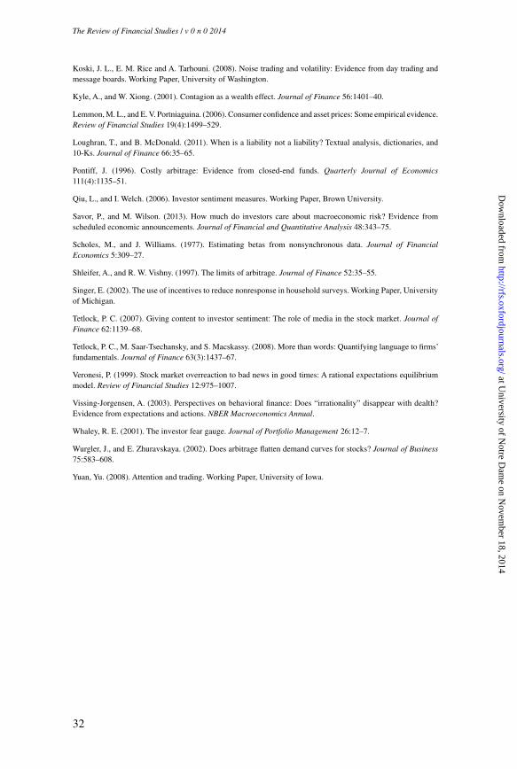
[11:32 28/10/2014 RFS-hhu072.tex] Page: 32 1–34


Koski, J. L., E. M. Rice and A. Tarhouni. (2008). Noise trading and volatility: Evidence from day trading andmessage boards. Working Paper, University of Washington.

Kyle, A., and W. Xiong. (2001). Contagion as a wealth effect. Journal of Finance 56:1401–40.

Lemmon, M. L., and E. V. Portniaguina. (2006). Consumer confidence and asset prices: Some empirical evidence.Review of Financial Studies 19(4):1499–529.

Loughran, T., and B. McDonald. (2011). When is a liability not a liability? Textual analysis, dictionaries, and10-Ks. Journal of Finance 66:35–65.

Pontiff, J. (1996). Costly arbitrage: Evidence from closed-end funds. Quarterly Journal of Economics111(4):1135–51.

Qiu, L., and I. Welch. (2006). Investor sentiment measures. Working Paper, Brown University.

Savor, P., and M. Wilson. (2013). How much do investors care about macroeconomic risk? Evidence fromscheduled economic announcements. Journal of Financial and Quantitative Analysis 48:343–75.

Scholes, M., and J. Williams. (1977). Estimating betas from nonsynchronous data. Journal of FinancialEconomics 5:309–27.

Shleifer, A., and R. W. Vishny. (1997). The limits of arbitrage. Journal of Finance 52:35–55.

Singer, E. (2002). The use of incentives to reduce nonresponse in household surveys. Working Paper, Universityof Michigan.

Tetlock, P. C. (2007). Giving content to investor sentiment: The role of media in the stock market. Journal ofFinance 62:1139–68.

Tetlock, P. C., M. Saar-Tsechansky, and S. Macskassy. (2008). More than words: Quantifying language to firms’fundamentals. Journal of Finance 63(3):1437–67.

Veronesi, P. (1999). Stock market overreaction to bad news in good times: A rational expectations equilibriummodel. Review of Financial Studies 12:975–1007.

Vissing-Jorgensen, A. (2003). Perspectives on behavioral finance: Does “irrationality” disappear with dealth?Evidence from expectations and actions. NBER Macroeconomics Annual.

Whaley, R. E. (2001). The investor fear gauge. Journal of Portfolio Management 26:12–7.

Wurgler, J., and E. Zhuravskaya. (2002). Does arbitrage flatten demand curves for stocks? Journal of Business75:583–608.

Yuan, Yu. (2008). Attention and trading. Working Paper, University of Iowa.

32

at University of N

otre Dam

e on Novem


Dow

nloaded from


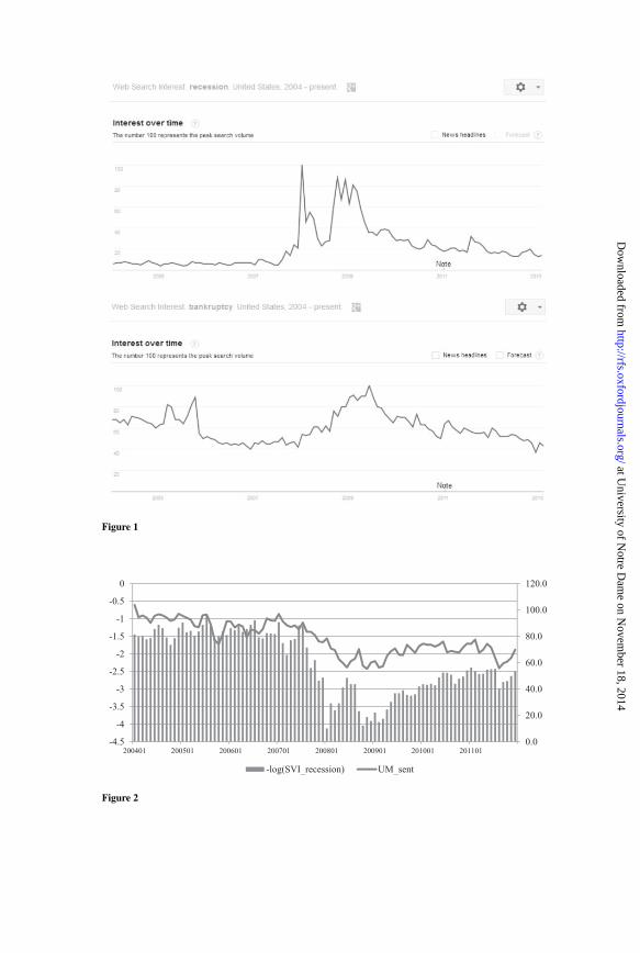
[11:32 28/10/2014 RFS-hhu072.tex] Page: 33 1–34

Figure 1

0.0

20.0

40.0

60.0

80.0

100.0

120.0

-4.5

-4

-3.5

-3

-2.5

-2

-1.5

-1

-0.5

0

200401 200501 200601 200701 200801 200901 201001 201101

-log(SVI_recession) UM_sent

Figure 2

at University of N

otre Dam

e on Novem


Dow

nloaded from


Documents

The Sum of All FEARS Investor Sentiment and Asset Priceszda/FEARS.pdf · The Sum of All FEARS Investor Sentiment and Asset Prices ... Rady School of Management, ... (FEARS) index