The subselect R package - Cran

The subselect R package

Jorge Cadima, Jorge Orestes Cerdeira, Pedro Duarte Silva, Manuel Minhoto

January 29, 2018

Version 0.12

Abstract

The subselect package addresses the issue of variable selection in different statistical contexts,among which exploratory data analyses; univariate or multivariate linear models; generalized linearmodels; principal components analysis; linear discriminant analysis, canonical correlation analysis.Selecting variable subsets requires the definition of a numerical criterion which measures the qualityof any given variable subset as a surrogate for the full set of variables. The current version ofthe subselect package provides eight different criteria. For each available criterion, the packageprovides a function that computes the criterion value of any given subset. More significantly, thepackage provides efficient search functions that seek the best subsets of any given size, for a specifiedcriterion.

Contents

1 Introduction 21.1 The variable selection problem . . . . . . . . . . . . . . . . . . . . . . . . . . . . . . . 21.2 Measuring the quality of a subset . . . . . . . . . . . . . . . . . . . . . . . . . . . . . . 21.3 Selecting the best subsets . . . . . . . . . . . . . . . . . . . . . . . . . . . . . . . . . . 21.4 Installing and loading subselect . . . . . . . . . . . . . . . . . . . . . . . . . . . . . . 3

2 Criteria for variable selection 32.1 Criteria for exploratory data analyses and PCA . . . . . . . . . . . . . . . . . . . . . . 3

2.1.1 The RM coefficient . . . . . . . . . . . . . . . . . . . . . . . . . . . . . . . . . . 42.1.2 The GCD coefficient . . . . . . . . . . . . . . . . . . . . . . . . . . . . . . . . . 62.1.3 The RV coefficient . . . . . . . . . . . . . . . . . . . . . . . . . . . . . . . . . . 7

2.2 Criteria for a Multivariate Linear model context . . . . . . . . . . . . . . . . . . . . . 82.2.1 Four criteria . . . . . . . . . . . . . . . . . . . . . . . . . . . . . . . . . . . . . 92.2.2 Creating the SSCP matrices . . . . . . . . . . . . . . . . . . . . . . . . . . . . . 102.2.3 The ccr2

1 (ccr12) coefficient and Roy’s first root statistic . . . . . . . . . . . . . 142.2.4 The τ2 (tau2) coefficient and Wilk’s Lambda . . . . . . . . . . . . . . . . . . . 152.2.5 The ξ2 (xi2) coefficient and the Bartlett-Pillai statistic . . . . . . . . . . . . . . 152.2.6 The ζ2 (zeta2) coefficient and the Lawley-Hotelling statistic . . . . . . . . . . . 16

2.3 Criterion for generalized linear models . . . . . . . . . . . . . . . . . . . . . . . . . . . 162.3.1 A helper function for the GLM context . . . . . . . . . . . . . . . . . . . . . . 172.3.2 Function wald.coef and the Wald coefficient . . . . . . . . . . . . . . . . . . . 18

1

3 Search algorithms 183.1 Common input arguments . . . . . . . . . . . . . . . . . . . . . . . . . . . . . . . . . . 193.2 Common output objects . . . . . . . . . . . . . . . . . . . . . . . . . . . . . . . . . . . 193.3 The eleaps function: an efficient complete search . . . . . . . . . . . . . . . . . . . . . 203.4 The anneal function: a simulated annealing algorithm . . . . . . . . . . . . . . . . . . 253.5 The genetic function: a genetic algorithm . . . . . . . . . . . . . . . . . . . . . . . . . 283.6 The improve function: a restricted improvement algorithm . . . . . . . . . . . . . . . 31

1 Introduction

1.1 The variable selection problem

Selecting a subset of variables which can be used as a surrogate for a full set of variables, withoutmajor loss of quality, is a problem that arises in numerous contexts.

Multiple linear regression has been the classical statistical setting for variable selection and thegreedy algorithms of backward elimination, forward selection and stepwise selection have long beenused to choose a subset of linear predictors. However, their limitations are well known and moreefficient search algorithms have also been devised, such as Furnival and Wilson’s Leaps and BoundsAlgorithm (reference [6]).

The subselect package addresses the issue of variable selection in different statistical contexts,among which:

• exploratory data analyses;

• univariate or multivariate linear models;

• generalized linear models;

• principal components analysis;

• linear discriminant analysis;

• canonical correlation analysis.

1.2 Measuring the quality of a subset

Selecting variable subsets requires the definition of a numerical criterion which measures the qualityof any given variable subset. In a univariate multiple linear regression, for example, possible measuresof the quality of a subset of predictors are the coefficient of determination R2, the F statistic in agoodness-of-fit test, its corresponding p-value or Akaike’s Information Criterion (AIC), to give a fewexamples.

The subselect package assumes that all potential variable subsets can be ranked according to awell-defined numerical criterion that is relevant for the problem at hand, and that the ultimate goalis to select the best subsets for any given cardinality, i.e., the subsets of any given size which have thehighest criterion values, for a given criterion.

The criteria currently available in the package will be further discussed in Section 2. For eachavailable criterion, the package provides a function that computes the criterion value of any givensubset. More importantly, the package provides efficient functions to search for the best subsets ofany given size.

1.3 Selecting the best subsets

Identifying the best variable subsets of a given cardinality is – for many criteria – a computation-ally intensive problem with datasets of even moderate size, as is well known in the standard linearregression context.

The subselect package has a function (eleaps) implementing Duarte Silva’s adaptations (refer-ences [4] and [5]) of Furnival and Wilson’s Leaps and Bounds Algorithm [6] for variable selection,

2

using the criteria considered in this package. This function is very fast for datasets with up to ap-proximately p = 30 variables and is guaranteed to identify the m best subsets of any size k from 1 top, with m in the range from 1 to

(pk

). It is the recommended function for variable selection

with small or moderately-sized data sets and is discussed in subsection 3.3.For larger data sets (roughly p > 35) the eleaps function is no longer computationally feasible

and alternative search heuristics are needed. The subselect package provides three functions withdifferent search algorithms:

anneal a simulated annealing-type search algorithm;

genetic a genetic algorithm; and

improve a modified local improvement algorithm.

These algorithms are described in reference [1] and are discussed in Section 3. They perform betterthan the greedy-type algorithms, such as the standard stepwise selection algorithms widely used inlinear regression.

All four search functions invoke code written in either C++ (eleaps) or Fortran (anneal, geneticand improve), to speed up computation times. The search functions are further discussed in Section3.

1.4 Installing and loading subselect

The subselect package is on CRAN (cran.r-project.org) and can be installed like any other CRANpackage, namely using R’s install.packages facility:

> install.packages(``subselect'')

This vignette assumes that the subselect package has already been installed in the user’s system.Once installed, subselect must be loaded into an R session:

> library(subselect)

A preliminary view of the available functions and of their purpose can, as usual, be obtained via:

> library(help=subselect)

2 Criteria for variable selection

Currently, the package accepts eight different criteria measuring the quality of any given variablesubset. These criteria can be (simplistically) classified into three groups: (i) criteria that are usefulin an exploratory analysis or principal component analysis of a data set; (ii) criteria that are model-based and are relevant in contexts that can be framed as a multivariate linear model (multivariatelinear regressions, MANOVAs, linear discriminant analysis, canonical correlation analysis, etc.); and(iii) criteria that are useful for variable selection in the context of a generalized linear model.

2.1 Criteria for exploratory data analyses and PCA

The three criteria relevant for exploratory data analyses have been previously suggested in the liter-ature (see references [2] and [1] for a fuller discussion). They can all be framed as matrix correlations[16] involving an n × p data matrix (where p is the number of variables and n the number of obser-vations on those variables) and projections of its columns on some subspace of Rn. In the subselect

package, these three criteria are called:

RM The square of this matrix correlation is the proportion of total variance (inertia) that is preservedif the p variables are orthogonally projected onto the subspace spanned by a given k-variablesubset. Choosing the k-variable subset that maximizes this criterion is therefore akin to whatis done in a Principal Component Analysis, with the difference that the optimal k-dimensionalsubspace is chosen only from among the

(pk

)subspaces spanned by k of the p variables. This is

3

the second of McCabe’s four criteria for what he terms principal variables [13]. See Subsection2.1.1 for more details.

GCD Yanai’s Generalized Coefficient of Determination [16] is a measure of the closeness of twosubspaces that is closely related to the gap metric [7]. More precisely, it is the average of thesquared canonical correlations between two sets of variables spanning each of the subspaces [16].In this context, these subspaces are the subspace spanned by g Principal Components of the full,p-variable, data set; and the subspace spanned by a k-variable subset of those p variables. Bydefault the PCs considered are the first g PCs, and the number of variables and PCs consideredis the same (k = g), but other options can be specified by the user. Maximizing the GCDcorresponds to chosing the k variables that span a subspace that is as close as possible to theprincipal subspace spanned by the g principal components that were specified. See Subsection2.1.2 for more details.

RV Escoufier’s RV-criterion [18] measures the similarity of the n-point configurations defined by then rows of two (comparable) data matrices, allowing for translations of the origin, rigid rotationsand global changes of scale. In this case, the two matrices that are compared are the originaldata matrix X and the matrix PkX which results from projecting the p columns of X ontoa k-dimensional subspace spanned by k of the p original variables. Maximizing this criterion,among all k-variable subsets, corresponds to choosing the k variables that span the subspacewhich best reproduces the original n-point configuration, allowing for translations of the origin,rigid rotations and global changes of scale. See Subsection 2.1.3 for more details.

The package functions that compute the values of these indices (described below) all have thefollowing two input arguments:

mat denotes the covariance or correlation matrix of the full data set;

indices is the vector, matrix or 3-d array of integers giving sets of integers identifying the variablesin the subsets of interest.

The function for the GCD coefficient has an additional argument, described in subsection 2.1.2.

2.1.1 The RM coefficient

Motivation and definition

It is well-known that the first k principal components of an n × p data set are the k linearcombinations of the p original variables which span the subspace that maximizes the proportion oftotal variance retained, if the data are orthogonally projected onto that subspace. A similar problem,but considering only the subspaces that are spanned by k-variable subsets of the p original variables,can be formulated [2] as follows: determine the k-variable subset which maximizes the square of theRM coefficient,

RM = corr(X,PkX) =

√tr(XtPkX)

tr(XtX)=

√√√√√√√p∑

i=1

λi(rm)2i

p∑j=1

λj

=

√tr([S2](K)S

−1K )

tr(S), (1)

with corr denoting the matrix correlation; tr the matrix trace; and where

• X is the full (column-centered or possibly standardized) data matrix;

• Pk is the matrix of orthogonal projections on the subspace spanned by a given k-variable subset;

• S = 1nXtX is the p× p covariance (or correlation) matrix of the full data set;

• K denotes the index set of the k variables in the variable subset;

• SK is the k× k principal submatrix of matrix S which results from retaining the rows/columnswhose indices belong to K;

4

• [S2](K) is the k×k principal submatrix of S2 obtained by retaining the rows/columns associatedwith set K.

• λi stands for the i-th largest eigenvalue of the covariance (or correlation) matrix defined by X;

• rm stands for the multiple correlation between the i-th principal component of the full data setand the k-variable subset.

The values of the RM coefficient will lie in the interval [0, 1], with larger values indicating a higherproportion of explained variance. Note that it is not relevant whether sample (co)variances (withdenominator n−1), or even the sums of squares and products matrices, are used instead of matrix Sas defined above: RM is insensitive to multiplication of S by a constant.

The rm.coef function

The subselect package provides the function rm.coef which computes the RM coefficient, given apositive definite matrix (function argument mat, corresponding to S in the final expression of equation(1)) and a vector with k indices (function argument indices, corresponding to K in (1)):

> rm.coef(mat,indices)

The rm.coef function uses the final expression in equation (1). In the standard setting, matrix Sis a covariance or correlation matrix for the full data set, but it may be any positive definite matrix,such as a matrix of non-central second moments.

Examples

As an example of the use of the rm.coef function, let us compute the value of the RM coefficientfor the two petal measurements in Fisher’s iris data (variables 3 and 4, respectively, Petal.Lengthand Petal.Width; see help(iris) in a standard R session for more information on this data set).This can be obtained as follows, using rm.coef ’s only two arguments:

> rm.coef(mat=var(iris[,-5]),indices=c(3,4))

[1] 0.9655367

>

The square of this value,

> rm.coef(var(iris[,-5]),c(3,4))^2

[1] 0.9322611

>

gives the proportion of total variability that is preserved if the four morphometric variables wereorthogonally projected onto the subspace spanned by the petal measurements. It is quite often thecase that this value is not very much smaller than the proportion of total variability that is accountedfor by the same number of principal components [2].

If more than one subset of a given cardinality is desired, the indices argument should be givenas a matrix whose rows provide the indices of the variables in each subset. For example, the RMcoefficients for the three-variable subsets of the iris data, given by variables 1, 2, 3 and 1, 2, 4 arerequested by the command:

> rm.coef(var(iris[,-5]), indices=matrix(nrow=2,ncol=3,byrow=TRUE,c(1,2,3,1,2,4)))

[1] 0.9960440 0.9890406

5

The argument indices can also be a three-dimensional array, if subsets of different cardinalitiesare desired. In this case, the third dimension of indices is associated with different cardinalities. Thisoption is especially useful when applying the rm.coef function to the output of the search algorithms(see Section 3), if more than one cardinality has been requested.

An example for the less frequent case, where the request is built from scratch, is now given. Itcomputes the value of RM for two 1-variable subsets and two 3-variable subsets:

> subsets <- array(data=c(3,2,0,0,0,0,1,1,2,2,3,4), dim=c(2,3,2))

> colnames(subsets) <- paste("V",1:3,sep="")

> rownames(subsets) <- paste("Solution",1:2)

> dimnames(subsets)[[3]]<-paste("Size",c(1,3))

> subsets

, , Size 1

V1 V2 V3

Solution 1 3 0 0

Solution 2 2 0 0

, , Size 3

V1 V2 V3

Solution 1 1 2 3

Solution 2 1 2 4

> rm.coef(var(iris[,-5]),indices=subsets)

Size 1 Size 3

Solution 1 0.9595974 0.9960440

Solution 2 0.4309721 0.9890406

The output places the values for each cardinality in a different column. Notice how the missingvariable indices for the lower cardinalities are given as zeroes,

2.1.2 The GCD coefficient


In the standard setting for the subselect package, given a p-variable data set and a subset of g ofits principal components, the GCD criterion is a measure of similarity between the principal subspacespanned by the g specified principal components and the subspace spanned by a given k-variablesubset of the original variables [2].

The GCD is the matrix correlation between the matrix Pk of orthogonal projections on thesubspace spanned by a given k-variable subset and the matrix Pg of orthogonal projections on thesubspace spanned by the g given principal components of the full data set [2]:

GCD = corr(Pk,Pg) =tr(Pk ·Pg)√

k · g=

1√kg

∑i∈G

(rm)2i = tr([SG](K)S

−1K )/

√gk, (2)

where

• K, S, SK and (rm)i are all defined as above (subsection 2.1.1);

• G denotes the index set of the g principal components in the PC subset;

• SG is the p × p matrix of rank g that results from retaining only the g terms in the spectraldecomposition of S that are associated with the PC indices in the set G;

• [SG](K) is the k×k principal submatrix of SG that results from retaining only the rows/columnswhose indices are in K.

6

The values of the GCD coefficient are in the interval [0, 1], with larger values indicating greatersimilarity between the subspaces.

The gcd.coef function

The gcd.coef function computes the GCD coefficient for a given positive definite matrix (functionargument mat, corresponding to matrix S in the final expression of equation (2)), a given vector of kvariable indices (function argument indices, corresponding to K in (2)), and a given vector of g PCindices (function argument pcindices, corresponding to G in (2)):

> gcd.coef(mat,indices,pcindices)

If the pcindices argument is not specified, by default it is set to the first k PCs, where k is thesize of the variable subset defined by argument indices.

The value of the GCD is computed using the final expression in equation (2). Matrix S (the inputargument mat) is usually the covariance or correlation matrix for the full p-variable data set, butthere may be other contexts where the final expression in (2) makes sense.

Examples

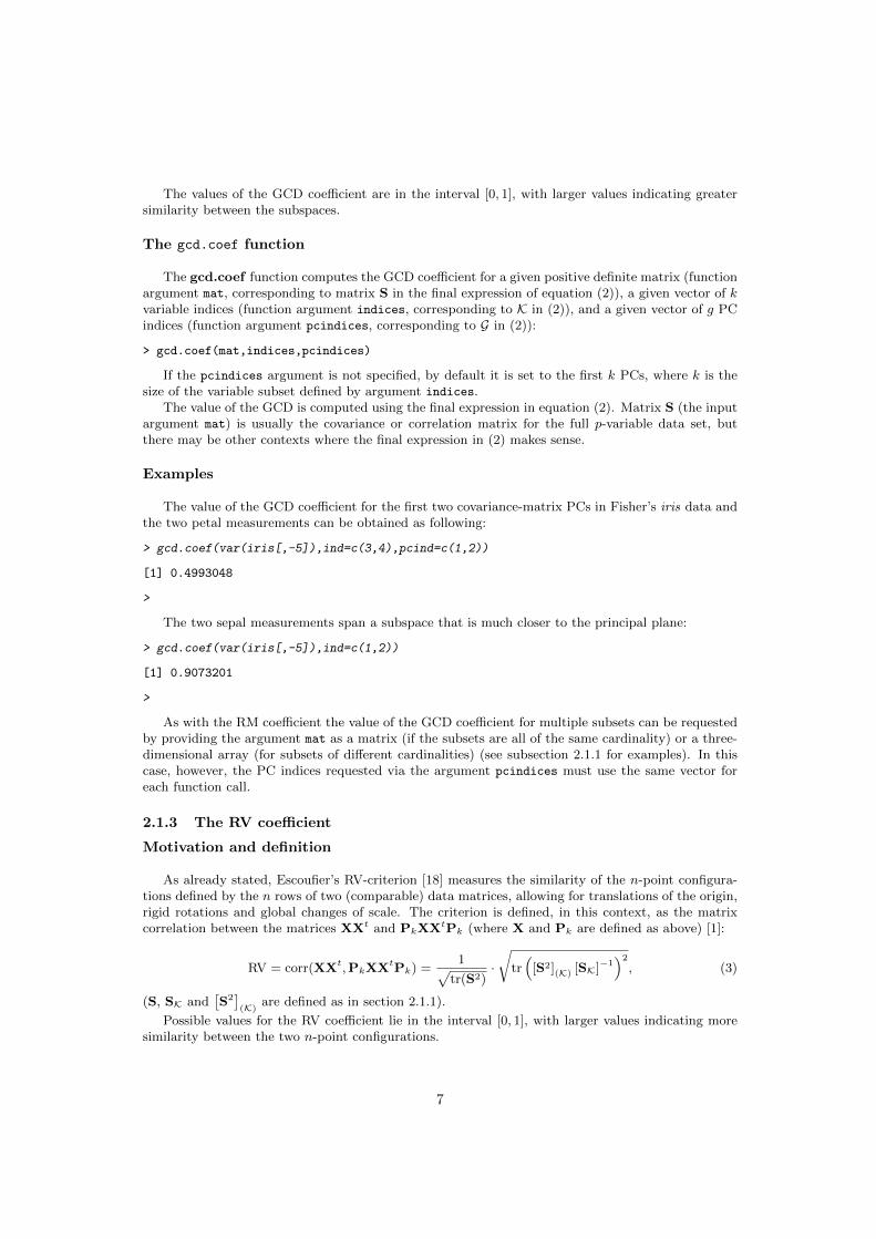
The value of the GCD coefficient for the first two covariance-matrix PCs in Fisher’s iris data andthe two petal measurements can be obtained as following:

> gcd.coef(var(iris[,-5]),ind=c(3,4),pcind=c(1,2))

[1] 0.4993048

>

The two sepal measurements span a subspace that is much closer to the principal plane:

> gcd.coef(var(iris[,-5]),ind=c(1,2))

[1] 0.9073201

>

As with the RM coefficient the value of the GCD coefficient for multiple subsets can be requestedby providing the argument mat as a matrix (if the subsets are all of the same cardinality) or a three-dimensional array (for subsets of different cardinalities) (see subsection 2.1.1 for examples). In thiscase, however, the PC indices requested via the argument pcindices must use the same vector foreach function call.

2.1.3 The RV coefficient


As already stated, Escoufier’s RV-criterion [18] measures the similarity of the n-point configura-tions defined by the n rows of two (comparable) data matrices, allowing for translations of the origin,rigid rotations and global changes of scale. The criterion is defined, in this context, as the matrixcorrelation between the matrices XXt and PkXXtPk (where X and Pk are defined as above) [1]:

RV = corr(XXt,PkXXtPk) =1√

tr(S2)·√

tr(

[S2](K) [SK]−1)2

, (3)

(S, SK and[S2](K)

are defined as in section 2.1.1).

Possible values for the RV coefficient lie in the interval [0, 1], with larger values indicating moresimilarity between the two n-point configurations.

7

The rv.coef function

The value of the RV coefficient, for a given positive definite matrix (function argument mat,corresponding to matrix S in the final expression of equation (3)) and a given vector of k variableindices (function argument indices, corresponding to K in equation (3)), can be computed using therv.coef function:

> rv.coef(mat,indices)

Examples

The farm data set (included in this package), has n = 99 individuals, observed in each of p = 62variables. The RV coefficient reveals that the 99−point configuration of the standardized data in R62

is fairly similar to the configuration that results from the orthogonal projection of those 99 points onthe subspace spanned by variables number 2, 37, 57 and 59:

> data(farm)

> rv.coef(cor(farm),ind=c(2,37,57,59))

[1] 0.8304743

For two different variable subsets of size 4, the argument indices is given as a matrix, whose rowsindicate the variable indices for each subset. For example, the RV-coefficients of the four-variablesubsets 2, 12, 56, 59 and 2, 3, 11, 59, are requested by the command:

> rv.coef(cor(farm), indices=matrix(nrow=2,ncol=4,byrow=TRUE,c(2,12,56,59,2,3,11,59)))

[1] 0.8315621 0.8295819

>

2.2 Criteria for a Multivariate Linear model context

Different statistical methods arise within the general framework of a multivariate linear model [9]:

X = AΨΨΨ + U,

where X is an n×p data matrix of original variables, A is a known (n×q) design matrix, ΨΨΨ is a (q×p)matrix of unknown parameters and U is a (n × p) matrix of error vectors. Particular cases in thissetting include, among others, [Multivariate] Analysis of Variance ([M]ANOVA), Linear DiscriminantAnalyis (LDA) and Canonical Correlation Analysis (CCA). Here we will be particularly concernedwith contexts where a selection of subsets of X is warranted, the classical cases being LDA and CCA.

In these statistical methods, variable subsets are often assessed according to their contribution tothe violation of an additional reference hypothesis, H0 : CΨΨΨ = 0, where C is a known coefficientmatrix of rank r [9].

For example, in LDA X is a matrix of n observations, divided by q groups, on p attributes; Ais a matrix of group indicators; and ΨΨΨ is a matrix of group-specific population means. In this case,the rows of C specify q− 1 contrasts, stating the equality of population means across groups. Hence,r = min(p, q − 1), and any index of the extent of H0 violations can be interpreted as a measure ofgroup separation.

In Canonical Correlation Analysis, A = [1n Y] where 1n is a vector of ones, the columns of Xand Y are n observations on two different sets of variables, the reference hypothesis, H0 : C ΨΨΨ =[0 Iq]

[ΨΨΨt

0 ΨΨΨtY

]t= 0, states that the two sets are uncorrelated, and r = min (rank(X), rank(Y)).

Indicators for the violation of H0 are measures of linear association between the X and Y variablesets. We note that in this context only the variables associated with the X group are selected, whilethe Y group of variables remains fixed.

When Y = y consists of a single (response) variable this problem becomes the traditional variableselection problem in Linear Regression, usually modelled as y = [1n X] [β0 βββX ]t +εεε. While subselect

8

can also be used with reasonable results in multivariate regression models Y = [1n X] [β0β0β0 βββX ]t + εεε,with Y having more than one column, the symmetric association indices considered in subselect

were not designed to measure the quality of Y predictions. In multivariate prediction problems other(non-symmetric) measures such as those discussed in Rencher [17] and McQuarrie and Tsai [14] maybe more relevant. In univariate regression all these measures are monotone functions of the traditionalcoefficient of determination, which is also the index considered by subselect.

It is well known that, under classical Gaussian assumptions, test statistics for H0 are given byseveral increasing functions of the r positive eigenvalues of a product matrix T−1H, with T and Hthe total and effect matrices of Sum of Squares and Cross Product (SSCP) deviations associated withH0, such that

T = H + E,

where matrix E is the matrix of residual SSCP. The former SSCP matrices are given by T = Xt(Ip−Pω)X and H = Xt(PΩ −Pω)X, where Ip is an identity matrix, PΩ = A(AtA)−At and

Pω = A(AtA)−At −A(AtA)−Ct[C(AtA)−Ct]−C(AtA)−At,

are projection matrices on the spaces spanned by the columns of A (space Ω) and by the linearcombinations of these columns that satisfy the reference hypothesis (space ω). In these formulas Mt

denotes the transpose of matrix M, and M− a generalized inverse. Furthermore, whether or notthe classical assumptions hold, the same eigenvalues can be used to define descriptive indices thatmeasure an ”effect” characterized by the violation of H0.

2.2.1 Four criteria

In the subselect package four effect-size indices, which are monotone functions of the traditionaltest statistics, are used as comparison criteria. These indices are called:

Ccr12 The ccr21 index is a function of the traditional Roy first root test statistic [19], λ1, for the

violation of the linear hypothesis of the form H0 : CΨΨΨ = 0. Maximizing this criterion isequivalent to maximizing Roy’s first root (see Subsection 2.2.3 for more details).

Tau2 The τ2 index is a function of the traditional Wilks’ Lambda statistic [20]. Maximizing thiscriterion is equivalent to minimizing Wilks’ Lambda (see Subsection 2.2.4).

Xi2 The ξ2 coefficient is a function of the Bartlett-Pillai trace test statistic [15] Maximizing thiscriterion is equivalent to maximizing the Bartlett-Pillai statistic (see Subsection 2.2.5).

Zeta2 The index ζ2 is a function of the traditional Lawley-Hotelling trace test statistic [12] [8]. Max-imizing this criterion is equivalent to maximizing the Lawley-Hotelling statistic (see Subsection2.2.6).

Cramer and Nicewander [3] introduced these indices in the context of CCA, and Huberty [9]discusses their use in the context of LDA and MANOVA. In all four cases, the indices are definedso that their values lie between 0 and 1, and the larger the index value, the better the variable subsetas a surrogate for the full data set. In the specific case of a multiple linear regression (with asingle response variable), all four indices are equal to the standard coefficient of determination, R2.However, in multivariate problems with r > 1 the indices differ because they place different emphasison canonical directions associated with the effect under study. In particular, ccr2

1 only considers thefirst canonical direction, ξ2 weights all r directions in a balanced way, and τ2, ζ2 are intermediateindices that emphasize the main directions (see reference [4] for further details).

The four package functions that compute the values of these indices are called *.coef, where theasterisk denotes the above criterion name. These functions have six input arguments:

mat denotes the Total SSCP matrix T;

H denotes the effects SSCP matrix of relevance for the particular case at hand (see subsection 2.2.2for more details);

r denotes the rank of the H matrix (except in degenerate cases - see the help files for each *.coef

function);

9

indices is the vector, matrix or 3-d array of integers that identify the variables in the subsets ofinterest;

tolval and tolsym are parameters used to check for ill-conditioning of the matrix mat, and thesymmetry of matrices mat and H (see the help files for more details).

2.2.2 Creating the SSCP matrices

The relevant Sum of Squares and Cross-Products Effect matrix H is specific to each context in whichmodel-based variable selection arises. Computing these matrices can sometimes be time-consumingand the direct application of the formulas described in the previous subsection can lead to largerounding errors. The subselect package provides helper functions which, for standard contexts, cre-ate both the SSCP Effects matrix H and the SSCP Total matrix T, using sound numerical proceduresbased on singular value decompositions, as well as computing the presumed rank r of H.

The output from these functions can be used as input for both the functions that compute themodel-based criteria of quality for a given variable subset (discussed in the subsections below) andfor the search functions that seek the best subsets of variables for a given data set (see Section 3).

For the multivariate linear model context, subselect provides three such helper functions. Forall three functions, the output is a list of four objects:

mat is the relevant Total SSCP matrix T divided by n − 1 (where n is the number of rows in thedata matrix);

H is the relevant Effect SSCP matrix divided by n− 1;

r is the rank of matrix H;

call is the function call which generated the output.

The fact that mat and T are not defined as the standard SSCP matrices, but rather divided byn− 1 is of no consequence, since multiplying T and H by a common scalar does not affect the criteriavalues.

The three helper functions currently available for the multivariate linear model context are thefollowing:

The lmHmat function for linear regression and CCA

The function lmHmat creates the necessary SSCP matrices for a linear regression or canonicalcorrelation analysis context. In a (possibly multivariate response) linear regression context, it isassumed that the response variables are fixed and a subset of the predictor variables is being assessed.In a canonical correlation analysis context, it is assumed that one of the two groups of variables isfixed, and it is a subset of the second group of variables that is being assessed (variable selection inboth groups will currently have to be done via a 2-step approach). This function takes by default thefollowing arguments:

x is a matrix containing the full set of predictor variables, in the regression context, or the group ofvariables in which a variable subset is to be chosen in the CCA context.

y is a matrix or vector containing the set of fixed response variables, in the regression context, orthe set of fixed variables in the CCA context.

There is an S3 method for arguments x and y of class data.frame, as well as methods for classesformula and lm, that replace the input arguments by:

formula a standard linear model formula y ∼ x1 + x2 + ... defining the model relation betweenresponse and predictor variables (in the regression context) or fixed and assessed variables inthe CCA context.

data a data frame from which variables specified in formula are preferentially to be taken.

or

fitdlmmodel an object of class lm, as produced by R’s lm function.

10

In this context, the output object mat is the covariance matrix Tx of the x variables; object H is thecovariance matrix Hx|y of the projections of the x variables on the space spanned by the y variables;and r is the expected rank of the H matrix which, under the assumption of linear independence,equals the minimum between the number of variables in the x and y sets (the true rank of H can bedifferent if the linear independence condition fails). See the lmHmat help file for more information.

Example. An example of the use of the helper function lmHmat involves the iris data set. Thegoal is to study the (univariate response) multiple linear regression of variable Sepal.Length

(the first variable in the iris data frame) on the three remaining predictors.

> lmHmat(x=iris[,2:4], y=iris[,1])

$mat

Sepal.Width Petal.Length Petal.Width

Sepal.Width 0.1899794 -0.3296564 -0.1216394

Petal.Length -0.3296564 3.1162779 1.2956094

Petal.Width -0.1216394 1.2956094 0.5810063

$H

Sepal.Width Petal.Length Petal.Width

Sepal.Width 0.00262602 -0.07886075 -0.03194931

Petal.Length -0.07886075 2.36822983 0.95945448

Petal.Width -0.03194931 0.95945448 0.38870928

$r

[1] 1

$call

lmHmat.data.frame(x = iris[, 2:4], y = iris[, 1])

The ldaHmat function for linear discriminant analysis

This function takes by default the following arguments:

x is a matrix containing the discriminating variables, from which a subset is being considered.

grouping is a factor specifying the class to which each observation belongs.

There are S3 methods for

• class data.frame input argument x;

• input object of class formula.

With these methods, the input arguments for ldaHmat can be given as:

formula a formula of the form grouping ∼ x1+x2+... where the x variables denote the discriminatingvariables.


In this context, the output objects mat and H are the standard total (T) and between-group(H) SSCP matrices of Fisher’s linear discriminant analysis; and output object r is the rank of thebetween-group matrix H, which equals the minimum between the number of discriminators and thenumber of groups minus one (although the true rank of H can be different, if the discriminators arelinearly dependent).

11

Examples A simple example of the use of function ldaHmat again involves the iris data set. Weseek to discriminate the three iris species, using the four morphometric variables as discriminators.

> ldaHmat(x=iris[,1:4], grouping=iris$Species)

$mat

Sepal.Length Sepal.Width Petal.Length Petal.Width

Sepal.Length 102.168333 -6.322667 189.8730 76.92433

Sepal.Width -6.322667 28.306933 -49.1188 -18.12427

Petal.Length 189.873000 -49.118800 464.3254 193.04580

Petal.Width 76.924333 -18.124267 193.0458 86.56993

$H


Sepal.Length 63.21213 -19.95267 165.2484 71.27933

Sepal.Width -19.95267 11.34493 -57.2396 -22.93267

Petal.Length 165.24840 -57.23960 437.1028 186.77400

Petal.Width 71.27933 -22.93267 186.7740 80.41333

$r

[1] 2

$call

ldaHmat.data.frame(x = iris[, 1:4], grouping = iris$Species)

In the same example, the function could have been invoked as:

> attach(iris)

> ldaHmat(Species ~ Sepal.Length + Sepal.Width + Petal.Length + Petal.Width)

$mat


Sepal.Length 102.168333 -6.322667 189.8730 76.92433

Sepal.Width -6.322667 28.306933 -49.1188 -18.12427

Petal.Length 189.873000 -49.118800 464.3254 193.04580

Petal.Width 76.924333 -18.124267 193.0458 86.56993

$H


Sepal.Length 63.21213 -19.95267 165.2484 71.27933

Sepal.Width -19.95267 11.34493 -57.2396 -22.93267

Petal.Length 165.24840 -57.23960 437.1028 186.77400

Petal.Width 71.27933 -22.93267 186.7740 80.41333

$r

[1] 2

$call

ldaHmat.formula(formula = Species ~ Sepal.Length + Sepal.Width +

Petal.Length + Petal.Width)

> detach(iris)

The glhHmat function for a general linear hypthesis context

The function glhHmat creates the appropriate SSCP matrices for any problem that can bedescribed as an instance of the general multivariate linear model X = AΨΨΨ +U, with a reference

12

hypothesis H0 : CΨΨΨ = 0, where ΨΨΨ is a matrix of unknown parameters and C is a known rank-rcoefficient matrix. By default, this function takes the following arguments:

x is a matrix containing the response variables.

A is a design matrix specifying a linear model in which X is the response.

C is a matrix or vector containing the coefficients of the reference hypothesis.

There is an S3 method for input of class data.frame in which x and A are defined as data frames.A further method accepts input of class formula, with input arguments:

formula a formula of the form X ∼ A1+A2+ ...+Ap where the terms of the right hand side specifythe relevant columns of the design matrix.

C a matrix or vector containing the coefficients of the reference hypothesis.


In this context, the T and H matrix have the generic form given at the beginning of this subsectionand r is the rank of H, which equals the rank of C (the true rank of H can be different from r if theX variables are linearly dependent).

Example. The following example creates the Total and Effects SSCP matrices, T and H, for ananalysis of the data set crabs in the MASS package. This data set records physical measurementson 200 specimens of Leptograpsus variegatus crabs observed on the shores of Western Australia. Thecrabs are classified by two factors, both with two levels each: sex and sp (crab species, as definedby its colour: blue or orange). The measurement variables include the carapace length (CL), thecarapace width (CW), the size of the frontal lobe (FL) and the rear width (RW). We assume that thereis an interest in comparing the subsets of these variables measured in their original and logarithmicscales. In particular, we assume that it is wished to create the T and H matrices associated withan analysis of the effect of the sp factor after controlling for sex. Only the formula, C and data

arguments are explicitly given in this function call.

> library(MASS)

> data(crabs)

> lFL <- log(crabs$FL) ; lRW <- log(crabs$RW); lCL <- log(crabs$CL); lCW <- log(crabs$CW)

> C <- matrix(0.,nrow=2,ncol=4)

> C[1,3] = C[2,4] = 1.

> C

[,1] [,2] [,3] [,4]

[1,] 0 0 1 0

[2,] 0 0 0 1

> Hmat5 <- glhHmat(cbind(FL,RW,CL,CW,lFL,lRW,lCL,lCW) ~ sp*sex,C=C,data=crabs)

> Hmat5

$mat

FL RW CL CW lFL lRW lCL

FL 1964.8964 1375.92420 4221.6722 4765.1928 131.977728 113.906076 138.315643

RW 1375.9242 1186.41150 2922.6779 3354.5236 93.560559 96.961292 97.428477

CL 4221.6722 2922.67790 9246.8527 10401.3878 285.023931 243.479136 303.358489

CW 4765.1928 3354.52360 10401.3878 11755.2667 322.144623 279.160241 341.776779

lFL 131.9777 93.56056 285.0239 322.1446 9.088336 7.905989 9.556135

lRW 113.9061 96.96129 243.4791 279.1602 7.905989 8.094783 8.273439

lCL 138.3156 97.42848 303.3585 341.7768 9.556135 8.273439 10.183194

lCW 137.6258 98.38041 300.6960 340.1509 9.503886 8.338091 10.097091

lCW

FL 137.625801

RW 98.380414

13

CL 300.696018

CW 340.150874

lFL 9.503886

lRW 8.338091

lCL 10.097091

lCW 10.050426

$H

FL RW CL CW lFL lRW

FL 85.205200 45.784800 176.247600 209.231400 5.7967443 3.45859277

RW 45.784800 170.046900 18.769500 74.965800 3.0238356 12.80782993

CL 176.247600 18.769500 404.216100 452.356800 12.0381364 1.43745463

CW 209.231400 74.965800 452.356800 523.442500 14.2580360 5.67260253

lFL 5.796744 3.023836 12.038136 14.258036 0.3944254 0.22844463

lRW 3.458593 12.807830 1.437455 5.672603 0.2284446 0.96467943

lCL 5.865986 1.190274 13.158093 14.909948 0.4003070 0.09041999

lCW 6.004088 2.653921 12.718332 14.891177 0.4088329 0.20062548

lCL lCW

FL 5.86598627 6.0040883

RW 1.19027431 2.6539211

CL 13.15809339 12.7183319

CW 14.90994753 14.8911765

lFL 0.40030704 0.4088329

lRW 0.09041999 0.2006255

lCL 0.43030750 0.4210740

lCW 0.42107404 0.4253378

$r

[1] 2

$call

glhHmat.formula(formula = cbind(FL, RW, CL, CW, lFL, lRW, lCL,

lCW) ~ sp * sex, C = C, data = crabs)

2.2.3 The ccr21 (ccr12) coefficient and Roy’s first root statistic


The ccr21 coefficient is an increasing function of Roy’s first root test statistic for the reference

hypothesis in the standard multivariate linear model. Roy’s first root is the largest eigenvalue ofHE−1, where H is the Effect matrix and E is the Error (residual) matrix. The index ccr2

1 is relatedto Roy’s first root λ1 by:

ccr21 =

λ1

1 + λ1.

The ccr12.coef function

The subselect package provides the function ccr12.coef which computes the ccr21 coefficient,

given the variance or total SSCP matrix for the full data set, mat, the effects SSCP matrix H, theexpected rank of the H matrix, r, and a vector indices with the indices of the variable subset that isbeing considered. These arguments may be defined with the helper functions described in Subsection2.2.2. A standard function call looks like:

> ccr12.coef(mat, H, r, indices)

For further arguments and options, see the function help page.

14

Example

The following example in the use of function ccr12.coef in the context of a (univariate response)Multiple Linear Regression uses the Cars93 data set from the MASS library. Variable 5 (average price)is regressed on 13 other variables. The goal is to compare subsets of these 13 variables according totheir ability to predict car prices. The helper function lmHmat creates the relevant input to test thevalue of the ccr2

1 criterion for the subset of the fourth, fifth, tenth and eleventh predictors.

> library(MASS)

> data(Cars93)

> CarsHmat <- lmHmat(x=Cars93[c(7:8,12:15,17:22,25)],y=Cars93[5])

> ccr12.coef(mat=CarsHmat$mat, H=CarsHmat$H, r=CarsHmat$r, indices=c(4,5,10,11))

[1] 0.7143794

2.2.4 The τ2 (tau2) coefficient and Wilk’s Lambda


The Tau squared index τ2 is a decreasing function of the standard Wilk’s Lambda statistic forthe multivariate linear model and its reference hypothesis. The Wilk’s lambda statistic (Λ) is givenby:

Λ =det(E)

det(T),

where E is the Error (residual) SSCP matrix and T is the Total SSCP matrix. The index τ2 is relatedto the Wilk’s Lambda statistic by:

τ2 = 1− Λ1/r,

where r is the rank of the Effect SSCP matrix H.

The tau2.coef function

Function tau2.coef is similar to its counterpart ccr12.coef described in the previous Subsection.A standard function call looks like:

> tau2.coef(mat, H, r, indices)

Example

A very simple example of the use of the τ2 criterion with the Linear Discriminant Analysis examplefor the iris data set, using all four morphometric variables to discriminate the three species. Thesubset consisting of variables 1 and 3 is then considered as a surrogate for all four variables.

> irisHmat <- ldaHmat(iris[1:4],iris$Species)

> tau2.coef(irisHmat$mat,H=irisHmat$H,r=irisHmat$r,c(1,3))

[1] 0.8003044

2.2.5 The ξ2 (xi2) coefficient and the Bartlett-Pillai statistic


The Xi squared index is an increasing function of the traditional Bartllet-Pillai trace test statistic.The Bartlett-Pillai trace P is given by: P = tr(HT−1) where H is the Effects SSCP matrix and Tis the Total SSCP matrix. The Xi squared index ξ2 is related to the Bartllet-Pillai trace by:

ξ2 =P

r,

where r is the rank of H.

15

The xi2.coef function

Function xi2.coef is similar to the previous criterion functions described in this Section. Astandard function call looks like:

> xi2.coef(mat, H, r, indices)

Example

The same example considered in Subsection 2.2.4, only this time using the ξ2 index of τ2.


> xi2.coef(irisHmat$mat,H=irisHmat$H,r=irisHmat$r,c(1,3))

[1] 0.4942503

2.2.6 The ζ2 (zeta2) coefficient and the Lawley-Hotelling statistic


The Zeta squared index ζ2 is an increasing function of the traditional Lawley-Hotelling trace teststatistic. The Lawley-Hotelling trace is given by V = tr(HE−1) where H is the Effect SSCP matrixand E is the Error SSCP matrix. The index ζ2 is related to the Lawley-Hotelling trace by:

ζ2 =V

V + r,

where r is the rank of H.

The zeta2.coef function

Again, function zeta2.coef has arguments similar to those of the other related functions in thisSection. A standard function call looks like:

> zeta2.coef(mat, H, r, indices)

Example

Again, the same example as in the previous two subsections:


> zeta2.coef(irisHmat$mat,H=irisHmat$H,r=irisHmat$r,c(1,3))

[1] 0.9211501

2.3 Criterion for generalized linear models


Variable selection in the context of generalized linear models is typically based on the minimiza-tion of statistics that test the significance of the excluded variables. In particular, the likelihood ratio,Wald and Rao statistics, or some monotone function of those statistics, are often proposed as com-parison criteria for variable subsets of the same dimensionality. All these statistics are asympoticallyequivalent and, given suitable assumptions, can be converted into information criteria, such as theAIC, which also compare subsets of different dimensionalities (see references [10] and [11] for furtherdetails).

Among these criteria, Wald’s statistic has some computational advantages because it can alwaysbe derived from the same maximum likelihood and Fisher information estimates (concerning the full

16

model). In particular, let Wall be the value of the Wald statistic testing the significance of the fullcovariate vector, b and F be the coefficient and Fisher information estimates, and H be an auxiliaryrank-one matrix given by H = FbbtF. It follows that the value of Wald’s statistic for the excludedvariables (Wexc) in a given subset is given by Wexc = Wall− tr(F−1

indicesHindices), where Findices andHindices are the portions of the F and H matrices associated with the selected variables.

The subselect package provides a function wald.coef that computes the value of Wald’s statis-tic, testing the significance of the excluded variables, in the context of variable subset selection ingeneralized linear models (see Subsection 2.3.2 for more details).

2.3.1 A helper function for the GLM context

As with the multivariate linear model context, creating the Fisher Information matrix and the auxil-iary matrix H described above may be time-consuming. The subselect package provides the helperfunction glmHmat which accepts a glm object (fitdglmmodel) to retrieve an estimate of Fisher’sInformation. (F) matrix together with an auxiliary rank-one positive-definite matrix (H), such thatthe positive eigenvalue of F−1H equals the value of Wald’s statistic for testing the global significanceof the fitted model. These matrices may be used as input to the function that computes the Waldcriterion, as well as to the variable selection search routines described in Section 3.

As an example of the use of this helper function, in the context of binary response logistic regressionmodels, consider the last 100 observations of the iris data set (retaining only observations for theversicolor and virginica species). Assume that the goal is to judge subsets of the four morphometricvariables (petal and sepal lengths and widths), in models with the binary response variable givenby an indicator variable of the two remaining species. The helper function glmHmat will producethe Fisher Information matrix (output object mat), the auxiliary H function (output object H), thefunction call, and set the rank of output object H to 1, as follows:

> iris2sp <- iris[iris$Species != "setosa",]

> modelfit <- glm(Species ~ Sepal.Length + Sepal.Width + Petal.Length +

+ Petal.Width, data=iris2sp, family=binomial)

> Hmat <- glmHmat(modelfit)

> Hmat

$mat


Sepal.Length 0.28340358 0.03263437 0.09552821 -0.01779067

Sepal.Width 0.03263437 0.13941541 0.01086596 0.04759284

Petal.Length 0.09552821 0.01086596 0.08847655 -0.01853044

Petal.Width -0.01779067 0.04759284 -0.01853044 0.03258730

attr(,"FisherI")

[1] TRUE

$H


Sepal.Length 0.11643732 0.013349227 -0.063924853 -0.050181400

Sepal.Width 0.01334923 0.001530453 -0.007328813 -0.005753163

Petal.Length -0.06392485 -0.007328813 0.035095164 0.027549918

Petal.Width -0.05018140 -0.005753163 0.027549918 0.021626854

$r

[1] 1

$call

glmHmat.glm(fitdglmmodel = modelfit)

17

2.3.2 Function wald.coef and the Wald coefficient

The function wald.coef computes the value (Wexc) of the Wald statistic, as described above. Thefunction takes as input arguments:

mat An estimate of Fisher’s information matrix F for the full model variable-coefficient estimates;

H A matrix product of the form H = FbbtF where b is a vector of variable-coefficient estimates;

indices a numerical vector, matrix or 3-d array of integers giving the indices of the variables in thesubset. If a matrix is specified, each row is taken to represent a different k -variable subset. If a3-d array is given, it is assumed that the third dimension corresponds to different cardinalities.

tolval and tolsym are parameters used in checks for ill-conditioning and positive-definiteness ofthe Fisher Information and the auxiliary (H) matrices (see the wald.coef help file for furtherdetails).

The values of arguments mat and H can be created using the glmHmat helper function, describedin subsection 2.3.1.

Example

An example of variable selection in the context of binary response regression models can be givenusing the same crabs data set from the MASS package that was already discussed in subsection 2.2.2.The logarithms and original physical measurements of the Leptograpsus variegatus crabs consideredin the MASS crabs data set are used to fit a logistic model where each crab’s sex forms the responsevariable. The quality of the variable subset made up by the first, sixth and seventh predictor variablesis measured via the Wald coefficent.

> library(MASS)

> lFL <- log(crabs$FL)

> lRW <- log(crabs$RW)

> lCL <- log(crabs$CL)

> lCW <- log(crabs$CW)

> logrfit <- glm(sex ~ FL + RW + CL + CW + lFL + lRW + lCL + lCW,data=crabs,family=binomial)

> lHmat <- glmHmat(logrfit)

> wald.coef(lHmat$mat,lHmat$H,indices=c(1,6,7),tolsym=1E-06)

[1] 2.286739

It should be stressed that, contrary to the criteria considered in the previous problems, Wexc isnot bounded above by 1 and Wexc is a decreasing function of subset quality.

3 Search algorithms

Given any data set for which the variable selection problem is relevant and a criterion that measureshow well any given variable subset approximates the full data set, the problem of finding the bestk-variable subsets for that criterion arises naturally. Such problems are computationally intensivefor the criteria considered in this package. A complete search, among all k-variable subsets is a taskwhich quickly becomes unfeasible even for moderately-sized data sets unless k is very small, or verylarge, when compared with p.

It may happen that a criterion has special properties which render enumeration methods possi-ble for some moderate-sized data sets. Furnival and Wilson’s [6] Leaps and bounds algorithm didthis in the context of subset selection in Linear Regression, and package co-author Duarte Silva (seereferences [4] and [5]) has discussed the application of this algorithm to various methods of Multivari-ate Statistics. The package function eleaps implements these algorithms for the criteria discussedabove, using C++ code (see Section 3.3). This function is very fast for small or moderately sizeddatasets (with roughly p < 30 variables). For larger data sets (roughly p > 35 variables) it becomescomputationally unfeasible and alternative search heuristics become necessary.

18

Traditional heuristics for the variable selection problem in the context of linear regression, suchas the backward elimination, forward selection or stepwise selection algorithms belong to a generalclass of algorithms called greedy. Their limitations are well-known. The search algorithms consideredin this package do not fall in this category. They are of three types: a simulated annealing algorithm(implemented by the anneal function and discussed in section 3.4); a genetic algorithm (functiongenetic, discussed in section 3.5) and a modified local search algorithm (function improve, discussedin section 3.6). These algorithms were discussed in [1]. The three corresponding package functionsuse Fortran code for computational efficiency.

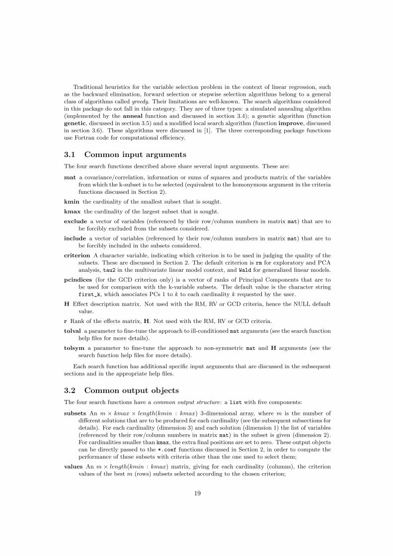
3.1 Common input arguments

The four search functions described above share several input arguments. These are:

mat a covariance/correlation, information or sums of squares and products matrix of the variablesfrom which the k-subset is to be selected (equivalent to the homonymous argument in the criteriafunctions discussed in Section 2).

kmin the cardinality of the smallest subset that is sought.

kmax the cardinality of the largest subset that is sought.

exclude a vector of variables (referenced by their row/column numbers in matrix mat) that are tobe forcibly excluded from the subsets considered.

include a vector of variables (referenced by their row/column numbers in matrix mat) that are tobe forcibly included in the subsets considered.

criterion A character variable, indicating which criterion is to be used in judging the quality of thesubsets. These are discussed in Section 2. The default criterion is rm for exploratory and PCAanalysis, tau2 in the multivariate linear model context, and Wald for generalized linear models.

pcindices (for the GCD criterion only) is a vector of ranks of Principal Components that are tobe used for comparison with the k-variable subsets. The default value is the character stringfirst_k, which associates PCs 1 to k to each cardinality k requested by the user.

H Effect description matrix. Not used with the RM, RV or GCD criteria, hence the NULL defaultvalue.

r Rank of the effects matrix, H. Not used with the RM, RV or GCD criteria.

tolval a parameter to fine-tune the approach to ill-conditioned mat arguments (see the search functionhelp files for more details).

tolsym a parameter to fine-tune the approach to non-symmetric mat and H arguments (see thesearch function help files for more details).

Each search function has additional specific input arguments that are discussed in the subsequentsections and in the appropriate help files.

3.2 Common output objects

The four search functions have a common output structure: a list with five components:

subsets An m × kmax × length(kmin : kmax) 3-dimensional array, where m is the number ofdifferent solutions that are to be produced for each cardinality (see the subsequent subsections fordetails). For each cardinality (dimension 3) and each solution (dimension 1) the list of variables(referenced by their row/column numbers in matrix mat) in the subset is given (dimension 2).For cardinalities smaller than kmax, the extra final positions are set to zero. These output objectscan be directly passed to the *.coef functions discussed in Section 2, in order to compute theperformance of these subsets with criteria other than the one used to select them;

values An m × length(kmin : kmax) matrix, giving for each cardinality (columns), the criterionvalues of the best m (rows) subsets selected according to the chosen criterion;

19

bestvalues A length(kmin : kmax) vector giving the overall best values of the criterion for eachcardinality;

bestsets A length(kmin : kmax) × kmax matrix, giving, for each cardinality (rows), the variables(referenced by their row/column numbers in matrix mat) in the best k-variable subset (can alsobe fed to the *.coef functions).

call The function call which generated the output.

3.3 The eleaps function: an efficient complete search

For each cardinality k (with k ranging from kmin to kmax), eleaps (”Extended Leaps and Bounds”)performs a branch and bound search for the best nsol-variable subsets (nsol being a user-specifiedfunction argument), according to a specified criterion. The function eleaps implements Duarte Silva’sadaptation for various multivariate analysis contexts (references [4] and [5]) of Furnival and Wilson’sLeaps and Bounds Algorithm (reference [6]) for variable selection in Regression Analysis. If the searchis not completed within a user defined time limit (input argument timelimit), eleaps exits with awarning message, returning the best (but not necessarly optimal) solutions found in the partial searchperformed.

In order to improve computation times, the bulk of computations are carried out by C++ routines.Further details about the Algorithm can be found in references [4] and [5] and in the comments tothe C++ code (in the package’s src directory). A discussion of the criteria considered can be foundin Section 2 above. The function checks for ill-conditioning of the input matrix (see the eleaps helpfile for details).

Examples

For illustration of use, we now consider five examples.

Example 1 deals with a small data set provided in the standard distributions of R. The swiss dataset is a 6-variable data set with Swiss fertility and socioeconomic indicators (1888). Subsets ofvariables of all cardinalities are sought, since the eleaps function sets, by default, kmin to 1and kmax to one less than the number of columns in the input argument mat. The function callrequests the best three subsets of each cardinality, using the RM criterion (subsection 2.1.1).

> data(swiss)

> eleaps(cor(swiss),nsol=3, criterion="RM")

$subsets

, , Card.1

Var.1 Var.2 Var.3 Var.4 Var.5

Solution 1 3 0 0 0 0



, , Card.2





, , Card.3



20



, , Card.4





, , Card.5





$values

card.1 card.2 card.3 card.4 card.5

Solution 1 0.6729689 0.8016409 0.9043760 0.9510757 0.9804629

Solution 2 0.6286185 0.7982296 0.8791856 0.9506434 0.9776338

Solution 3 0.6286130 0.7945390 0.8777509 0.9395708 0.9752551

$bestvalues

Card.1 Card.2 Card.3 Card.4 Card.5

0.6729689 0.8016409 0.9043760 0.9510757 0.9804629

$bestsets


Card.1 3 0 0 0 0

Card.2 3 6 0 0 0

Card.3 4 5 6 0 0

Card.4 2 4 5 6 0

Card.5 1 2 3 5 6

$call

eleaps(mat = cor(swiss), nsol = 3, criterion = "RM")

In this example, it is not necessary to explicitly specify the criterion RM, since it is the defaultcriterion for any function call which does not explicitly set the r input argument (except in aGLM context - see Section 2.3).

Example 2 illustrates the use of the include and exclude arguments that are common to all thesearch functions provided by the package subselect. Here, we request only 2- and 3- dimensionalsubsets that exclude variable number 6 and include variable number 1. For each cardinality, threesolutions are requested (argument nsol). The criterion requested is the GCD (see subsection2.1.2) and the subspace used to gauge our solutions is the principal subspace spanned by thefirst three principal components of the full data set (argument pcindices). Our solutions will bethe 2- and 3-variable subsets that span subspaces that are closest to this 3-d principal subspace.

> data(swiss)

> swiss.gcd <- eleaps(cor(swiss),kmin=2,kmax=3,exclude=6,include=1,nsol=3,criterion="gcd",pcindices=1:3)

> swiss.gcd

$subsets

, , Card.2

21

Var.1 Var.2 Var.3

Solution 1 1 5 0

Solution 2 1 4 0

Solution 3 1 2 0

, , Card.3

Var.1 Var.2 Var.3

Solution 1 1 4 5

Solution 2 1 2 5

Solution 3 1 3 5

$values

card.2 card.3

Solution 1 0.7124687 0.7930632

Solution 2 0.6281922 0.7920334

Solution 3 0.5934854 0.7381808

$bestvalues

Card.2 Card.3

0.7124687 0.7930632

$bestsets

Var.1 Var.2 Var.3

Card.2 1 5 0

Card.3 1 4 5

$call

eleaps(mat = cor(swiss), kmin = 2, kmax = 3, nsol = 3, exclude = 6,

include = 1, criterion = "gcd", pcindices = 1:3)

The output of this function call can be used as input for a function call requesting the values ofthe chosen solutions under a different criterion. For example, the values of the RM coefficientfor the above solutions are given by:

> rm.coef(mat=cor(swiss), indices=swiss.gcd$subsets)

Card.2 Card.3

Solution 1 0.7476013 0.8686515

Solution 2 0.7585398 0.8791856

Solution 3 0.7945390 0.8554279

Example 3 involves a Linear Discriminant Analysis example with a very small data set, whichhas already been discussed in subsection 2.2.4. We consider the Iris data and three groups,defined by species (setosa, versicolor and virginica). The goal is to select the 2- and 3-variablesubsets that are optimal for the linear discrimination (as measured by the ccr12 criterion, i.e.,by Roy’s first root statistic).


> eleaps(irisHmat$mat,kmin=2,kmax=3,H=irisHmat$H,r=irisHmat$r,crit="ccr12")

$subsets

, , Card.2

Var.1 Var.2 Var.3

Solution 1 1 3 0

22

, , Card.3

Var.1 Var.2 Var.3

Solution 1 2 3 4

$values

card.2 card.3

Solution 1 0.9589055 0.9678971

$bestvalues

Card.2 Card.3

0.9589055 0.9678971

$bestsets

Var.1 Var.2 Var.3

Card.2 1 3 0

Card.3 2 3 4

$call

eleaps(mat = irisHmat$mat, kmin = 2, kmax = 3, criterion = "ccr12",

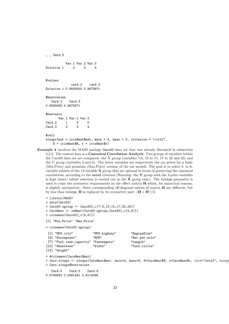
H = irisHmat$H, r = irisHmat$r)

Example 4 involves the MASS package Cars93 data set that was already discussed in subsection2.2.3. The context here is a Canonical Correlation Analysis. Two groups of variables withinthe Cars93 data set are compared: the X group (variables 7,8, 12 to 15, 17 to 22 and 25) andthe Y group (variables 4 and 6). The latter variables are respectively the car prices for a basic(Min.Price) and premium (Max.Price) version, of the car models. The goal is to select 4- to 6-variable subsets of the 13-variable X group that are optimal in terms of preserving the canonicalcorrelations, according to the zeta2 criterion (Warning: the Y group with the 2-price variablesis kept intact; subset selection is carried out in the X group only). The tolsym parameter isused to relax the symmetry requirements on the effect matrix H which, for numerical reasons,is slightly asymmetric. Since corresponding off-diagonal entries of matrix H are different, butby less than tolsym, H is replaced by its symmetric part: (H + Ht)/2.

> library(MASS)

> data(Cars93)

> Cars93.xgroup <- Cars93[,c(7:8,12:15,17:22,25)]

> CarsHmat <- lmHmat(Cars93.xgroup,Cars93[,c(4,6)])

> colnames(Cars93[,c(4,6)])

[1] "Min.Price" "Max.Price"

> colnames(Cars93.xgroup)

[1] "MPG.city" "MPG.highway" "EngineSize"

[4] "Horsepower" "RPM" "Rev.per.mile"

[7] "Fuel.tank.capacity" "Passengers" "Length"

[10] "Wheelbase" "Width" "Turn.circle"

[13] "Weight"

> #colnames(CarsHmat$mat)

> Cars.eleaps <- eleaps(CarsHmat$mat, kmin=4, kmax=6, H=CarsHmat$H, r=CarsHmat$r, crit="zeta2", tolsym=1e-9)

> Cars.eleaps$bestvalues

Card.4 Card.5 Card.6

0.5792692 0.5981441 0.6116096

23

> Cars.eleaps$bestsets

Var.1 Var.2 Var.3 Var.4 Var.5 Var.6

Card.4 4 5 10 11 0 0

Card.5 4 5 9 10 11 0

Card.6 4 5 9 10 11 12

Example 5. A final example involves the use of the eleaps function for variable selection in thecontext of a generalized linear model, more precisely, of a logistic regression model. Weconsider the last 100 observations of the iris data set (versicolor and virginica species) and seekthe best variable subsets for the model with the indicator variable for the other two species asthe binary response variable.


> logrfit <- glm(Species ~ Sepal.Length + Sepal.Width + Petal.Length + Petal.Width,iris2sp,family=binomial)

> Hmat <- glmHmat(logrfit)

> eleaps(Hmat$mat, H=Hmat$H, r=Hmat$r, criterion="Wald", nsol=3)

$subsets

, , Card.1

Var.1 Var.2 Var.3

Solution 1 4 0 0

Solution 2 1 0 0

Solution 3 3 0 0

, , Card.2

Var.1 Var.2 Var.3

Solution 1 1 3 0

Solution 2 3 4 0

Solution 3 2 4 0

, , Card.3

Var.1 Var.2 Var.3

Solution 1 2 3 4

Solution 2 1 3 4

Solution 3 1 2 3

$values

card.1 card.2 card.3

Solution 1 4.894554 3.522885 1.060121

Solution 2 5.147360 3.952538 2.224335

Solution 3 5.161553 3.972410 3.522879

$bestvalues


4.894554 3.522885 1.060121

$bestsets

Var.1 Var.2 Var.3

Card.1 4 0 0

Card.2 1 3 0

Card.3 2 3 4

24

$call

eleaps(mat = Hmat$mat, nsol = 3, criterion = "Wald", H = Hmat$H,

r = Hmat$r)

It should be stressed that, unlike other criteria in the subselect package, the Wald criterion isnot bounded above by 1 and is a decreasing function of subset quality, so that the 3-variablesubsets do, in fact, perform better than their smaller-sized counterparts.

3.4 The anneal function: a simulated annealing algorithm

Given a full data set, the anneal function uses a Simulated Annealing algorithm to seek a k-variablesubset which is optimal, as a surrogate for the full set, with respect to a given criterion. The algorithmis described in detail in [1].

In brief, for each of the solutions requested by the user (via the nsol function argument), an initialk-variable subset (for k ranging from kmin to kmax) of a full set of p variables is randomly selected andpassed on to a Simulated Annealing algorithm. The algorithm then selects a random subset in theneighbourhood of the current subset (neighbourhood of a subset S being defined as the family of allk-variable subsets which differ from S by a single variable), and decides whether to replace the currentsubset according to the Simulated Annealing rule, i.e., either (i) always, if the alternative subset’s

criterion value is larger; or (ii) with probability expac−cc

t if the alternative subset’s criterion value(ac) is smaller than that of the current solution (cc), where t (the temperature parameter) decreasesthroughout the iterations of the algorithm. For each cardinality k, the stopping criterion for thealgorithm is the number of iterations, which is controlled by the user (function argument niter).Also controlled by the user are the initial temperature (argument temp), the rate of geometric coolingof the temperature (argument cooling) and the frequency with which the temperature is cooled, asmeasured by argument coolfreq, the number of iterations after which the temperature is multipliedby 1-cooling.

Optionally, the best k-variable subset produced by the simulated annealing algorithm may beused as input in a restricted local search algorithm, for possible further improvement (this option iscontrolled by the logical argument improvement which, by default, is TRUE). The user may force vari-ables to be included and/or excluded from the k-variable subsets (arguments include and exclude),and may specify initial solutions (argument initialsol).

Computational effortFor each cardinality k, the total number of calls to the procedure which computes the criterion valuesis nsol×niter+1. These calls are the dominant computational effort in each iteration of the algorithm.In order to improve computation times, the bulk of computations is carried out by a Fortran routine.Further details about the Simulated Annealing algorithm can be found in reference [1] and in thecomments to the Fortran code (in the src subdirectory for this package).

The force argumentFor datasets with a very large number of variables (currently p > 400), it is necessary to set theforce argument to TRUE for the function to run, but this may cause a session crash if there is notenough memory available. The function checks for ill-conditioning of the input matrix (see details inthe anneal help file).

Reproducible solutionsThe anneal algorithm is a random algorithm, so that solutions are, in general, different each time thealgorithm is run. For reproducible solutions, the logical argument setseed should be set to TRUEduring a session and left as TRUE in subsequent function calls where it is wished to reproduce theresults.

Uniqueness of solutionsThe requested nsol solutions are not necessarily different solutions. The nsol solutions are computed

25

separately, so that (unlike what happens with the eleaps function), the same variable subset mayappear more than once among the nsol solutions.

ExamplesFour examples of usage of the anneal function are now given.

Example 1 is a very simple example, with a small data set with very few iterations of the algorithm,using the RM criterion (although for a data set of this size it is best to use the eleaps completesearch, described in section 3.3).

> data(swiss)

> anneal(cor(swiss),kmin=2,kmax=3,nsol=4,niter=10,criterion="RM")

$subsets

, , Card.2

Var.1 Var.2 Var.3

Solution 1 3 6 0

Solution 2 3 6 0

Solution 3 4 5 0

Solution 4 4 5 0

, , Card.3

Var.1 Var.2 Var.3

Solution 1 1 2 5

Solution 2 3 5 6

Solution 3 4 5 6

Solution 4 4 5 6

$values

card.2 card.3

Solution 1 0.8016409 0.8791856

Solution 2 0.8016409 0.8769672

Solution 3 0.7982296 0.9043760

Solution 4 0.7982296 0.9043760

$bestvalues

Card.2 Card.3

0.8016409 0.9043760

$bestsets

Var.1 Var.2 Var.3

Card.2 3 6 0

Card.3 4 5 6

$call

anneal(mat = cor(swiss), kmin = 2, kmax = 3, nsol = 4, niter = 10,

criterion = "RM")

Example 2 uses the 62-variable farm data set, included in this package (see help(farm) for details).

> data(farm)

> anneal(cor(farm), kmin=6, nsol=5, criterion="rv")

$subsets

, , Card.6

26


Solution 1 10 11 14 40 44 45

Solution 2 2 11 14 40 45 59

Solution 3 2 15 37 45 56 59

Solution 4 2 11 14 40 45 59

Solution 5 2 11 14 40 45 59

$values

card.6

Solution 1 0.8648286





$bestvalues

Card.6

0.865388

$bestsets


Card.6 2 11 14 40 45 59

$call

anneal(mat = cor(farm), kmin = 6, nsol = 5, criterion = "rv")

Since the kmax argument was not specified, the anneal function by default assigns it the samevalue as kmin. Notice that there may be repeated subsets among the 5 solutions produced bythe function call.

Example 3 involves subset selection in the context of a (univariate) Multiple Linear Regres-sion. The data set cystfibr, included in the ISwR package, contains lung function data forcystic fibrosis patients (7-23 years old). The data consists of 25 observations on 10 variables.The objective is to predict the variable pemax (maximum expiratory pressure) from relevant pa-tient characteristics. A best subset of linear predictors is sought, using the tau2 criterion which,in the case of a univariate linear regression, is just the standard Coefficient of Determination,R2.

> library(ISwR)

> cystfibrHmat <- lmHmat(pemax ~ age+sex+height+weight+bmp+fev1+rv+frc+tlc, data=cystfibr)

> colnames(cystfibrHmat$mat)

[1] "age" "sex" "height" "weight" "bmp" "fev1" "rv" "frc"

[9] "tlc"

> cystfibr.tau2 <- anneal(cystfibrHmat$mat, kmin=4, kmax=6, H=cystfibrHmat$H, r=cystfibrHmat$r, crit="tau2")

> cystfibr.tau2$bestvalues


0.6141043 0.6214494 0.6266394

> cystfibr.tau2$bestsets


Card.4 4 5 6 7 0 0

Card.5 4 5 6 7 9 0

Card.6 1 3 4 5 6 7

27

The algorithm underlying the anneal function is a random algorithm, whose solutions are notnecessarily reproducible. It may happen that the solutions for different cardinalities are notnested. This illustrates that the algorithm can produce different results from the standardgreedy algorithms, such as forward selection or backward elimination.

That the value of the τ2 coefficient in the context of a univariate linear regression is the coefficientof determination can be confirmed via R’s standard lm function:

> summary(lm(pemax ~ weight+bmp+fev1+rv, data=cystfibr))$r.squared

[1] 0.6141043

The other three multivariate linear hypothesis criteria discussed in Section 2.2 also give thevalue of R2 in a univariate multiple regression, as is illustrated by the following command,which requests the value of the ξ2 criterion for the above solutions.

> xi2.coef(mat=cystfibrHmat$mat, indices=cystfibr.tau2$bestsets, H=cystfibrHmat$H, r=cystfibrHmat$r)


0.6141043 0.6214494 0.6266394

Example 4 considers variable selection in the context of a logistic regression model. We considerthe last 100 observations of the iris data set (that is, the observations for the versicolor andvirginica species) and seek the best 1- to 3-variable subsets for the logistic regression that usesthe four morphometric variables to model the probability of each of these two species.

> data(iris)


> logrfit <- glm(Species ~ Sepal.Length + Sepal.Width + Petal.Length + Petal.Width,iris2sp,family=binomial)

> Hmat <- glmHmat(logrfit)

> iris2p.Wald <- anneal(Hmat$mat,1,3,H=Hmat$H,r=1,nsol=5,criterion="Wald")

> iris2p.Wald$bestsets

Var.1 Var.2 Var.3

Card.1 4 0 0

Card.2 1 3 0

Card.3 2 3 4

> iris2p.Wald$bestvalues


4.894554 3.522885 1.060121

3.5 The genetic function: a genetic algorithm

Given a full data set, a Genetic Algorithm algorithm seeks a k-variable subset which is optimal, as asurrogate for the full set, with respect to a given criterion. The algorithm is described in detail in [1].

In brief, for each cardinality k (with k ranging from the function arguments kmin to kmax), aninitial population of k-variable subsets is randomly selected from a full set of p variables. The size ofthis initial population is specified by the function argument popsize (popsize=100 by default). Ineach iteration, popsize/2 couples are formed from among the population and each couple generatesa child (a new k-variable subset) which inherits properties of its parents (specifically, it inherits allvariables common to both parents and a random selection of variables in the symmetric differenceof its parents’ genetic makeup). Each offspring may optionally undergo a mutation in the form ofa local improvement algorithm (see subsection 3.6), with a user-specified probability. Whether ornot mutations occur is controlled by the logical variable mutate (which is FALSE by default), andthe respective probability is given by the argument mutprob. The parents and offspring are rankedaccording to their criterion value, and the best popsize of these k-subsets will make up the nextgeneration, which is used as the current population in the subsequent iteration.

The stopping rule for the algorithm is the number of generations, which is specified by the functionargument nger.

28

Optionally, the best k -variable subset produced by the Genetic Algorithm may be passed as inputto a restricted local improvement algorithm, for possible further improvement (see subsection 3.6).

The user may force variables to be included and/or excluded from the k -subsets (function argu-ments include and exclude), and may specify an initial population (function argument initialpop).

The function checks for ill-conditioning of the input matrix (see the genetic help file for details).

Genetic diversityFor this algorithm to run, it needs genetic diversity in the population (i.e., a large number of differentvariables in the variable subsets that are being considered). This means that the function will not runon data sets with a small number of variables, p. In an attempt to ensure this genetic diversity, thefunction has an optional argument maxclone, which is an integer variable specifying the maximumnumber of identical replicates (clones) of individuals (variable subsets) that is acceptable in thepopulation. However, even maxclone=0 does not guarantee that there are no repetitions: only theoffspring of couples are tested for clones. If any such clones are rejected, they are replaced by ak-variable subset chosen at random, without any further clone tests.

Computational effortFor each cardinality k, the total number of calls to the procedure which computes the criterion valuesis popsize + nger × popsize/2. These calls are the dominant computational effort in each iterationof the algorithm. In order to improve computation times, the bulk of computations are carried outby a Fortran routine. Further details about the Genetic Algorithm can be found in [1] and in thecomments to the Fortran code (in the src subdirectory for this package).

The force argumentFor datasets with a very large number of variables (currently p > 400), it is necessary to set the force

argument to TRUE for the function to run, but this may cause a session crash if there is not enoughmemory available.

Reproducible solutionsThe genetic algorithm is a random algorithm, so that solutions are, in general, different each timethe algorithm is run. For reproducible solutions, the logical argument setseed should be set to TRUEduring a session and left as TRUE in subsequent function calls where it is wished to reproduce theresults.

Uniqueness of solutionsThe requested nsol solutions are not necessarily different solutions. The nsol solutions are computedseparately, so that (unlike what happens with the eleaps function), the same variable subset mayappear more than once among the nsol solutions.

ExamplesTwo examples of use of the genetic function are now given:

Example 1. Consider the 62-variable Portuguese farm dataset, already discussed in subsection 2.1.3(page 7). We seek a 10-variable subset which spans a subspace as close as possible to the first10-d principal subspace, so that criterion GCD (subsection 2.1.2) is relevant. By default, in thegenetic function (as in the anneal and improve function, but unlike the eleaps function), thedefault value of kmax is set equal to the value of kmin, and so does not need to be specified inthis case.

> farm.gcd <- genetic(cor(farm), kmin=10, crit="gcd")

> farm.gcd$bestsets

Var.1 Var.2 Var.3 Var.4 Var.5 Var.6 Var.7 Var.8 Var.9 Var.10

Card.10 14 28 30 31 38 39 40 44 46 60

> farm.gcd$bestvalues

29

Card.10

0.7941187

Since the argument popsize was not specified, the default population size (100) was used. Asstated above, not all 100 solutions are necessarily different. To select only the different solutionsR’s function unique may be used:

> unique(farm.gcd$subsets)

, , Card.10

Var.1 Var.2 Var.3 Var.4 Var.5 Var.6 Var.7 Var.8 Var.9 Var.10

Solution 1 11 14 29 30 31 38 39 40 44 59

Solution 7 14 29 30 31 38 39 40 44 45 59

Solution 13 11 29 30 31 37 38 39 40 44 59

Solution 19 14 29 30 38 39 40 44 45 48 59

Solution 25 11 14 29 31 38 39 40 44 47 59

Solution 31 14 29 30 31 38 39 40 44 57 59

Solution 37 14 29 31 38 39 40 44 45 47 59

Solution 43 11 29 31 37 38 39 40 44 47 59

Solution 49 14 29 38 39 40 44 45 47 48 59

Solution 55 29 30 31 37 38 39 40 44 45 59

Solution 61 14 29 31 38 39 40 44 47 57 59

Solution 67 29 30 31 37 38 39 40 44 57 59

Solution 73 14 29 30 38 39 40 44 48 57 59

Solution 79 14 25 29 30 31 38 39 40 44 45

Solution 85 29 30 37 38 39 40 44 45 48 59

Solution 91 11 14 29 30 38 39 40 44 48 59

Solution 97 29 31 37 38 39 40 44 45 47 59

Solution 103 11 14 25 29 30 31 38 39 40 44

Solution 109 14 25 29 30 38 39 40 44 45 48

Solution 115 11 29 30 37 38 39 40 44 48 59

Solution 121 29 31 37 38 39 40 44 47 57 59

If more than just a few different solutions are desired, it may be possible to increase the diversityof solutions by using the maxclone argument. The following example compares the number ofdifferent solutions obtained using the default value of maxclone=5 and a user-specified valuemaxclone=0. Since the subsets output object is a 3-d array, unique also produces a 3-d object,whose first dimension gives the number of different solutions.

> dim(unique(genetic(cor(farm), kmin=10, crit="gcd")$subsets))

[1] 22 10 1

> dim(unique(genetic(cor(farm), kmin=10, maxclone=0, crit="gcd")$subsets))

[1] 124 10 1

Example 2. We consider subset selection in the context of a Canonical Correlation Analysis.The data set in this example is the same as in Example 1 above. Two groups of variables withinthe farm data set are compared: the X group (all variables except the first four) and the Ygroup (variables 1 to 4). The goal is to select 4- to 6-variable subsets of the 58-variable Xgroup that are optimal in terms of preserving the canonical correlations, according to the zeta2

criterion. (Warning: the 4-variable Y group is kept intact; subset selection is carried out in theX group only). As can be seen from the results, even a four-variable X subgroup essentiallyreproduces the canonical correlations with the Y group of variables

> data(farm)

> farm.xgroup <- farm[,-c(1,2,3,4)]

> farmHmat <- lmHmat(farm.xgroup,farm[,1:4])

> colnames(farmHmat$mat)

30

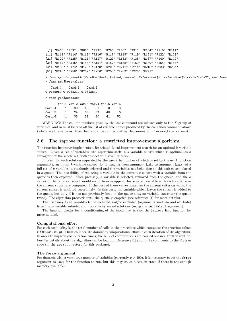
[1] "R46" "R59" "R65" "R72" "R79" "R86" "R91" "R104" "R110" "R111"

[11] "R113" "R114" "R115" "R116" "R117" "R118" "R119" "R121" "R122" "R123"

[21] "R124" "R125" "R126" "R127" "R129" "R132" "R135" "R137" "R140" "R142"

[31] "R144" "R145" "R146" "R151" "R152" "R158" "R159" "R160" "R164" "R166"

[41] "R168" "R174" "R176" "R178" "R209" "R211" "R214" "R215" "R233" "R237"

[51] "R245" "R250" "R252" "R256" "R258" "R263" "R270" "R271"

> farm.gen <- genetic(farmHmat$mat, kmin=4, kmax=6, H=farmHmat$H, r=farmHmat$r,crit="zeta2", maxclone=0, popsize=150)

> farm.gen$bestvalues


0.9165989 0.9262310 0.9342642

> farm.gen$bestsets


Card.4 1 39 40 51 0 0

Card.5 1 24 33 39 40 0

Card.6 1 33 39 40 41 52

WARNING: The column numbers given by the last command are relative only to the X group ofvariables, and so must be read off the list of variable names produced by the colnames command above(which are the same as those that would be printed out by the command colnames(farm.xgroup)).

3.6 The improve function: a restricted improvement algorithm

The function improve implements a Restricted Local Improvement search for an optimal k-variablesubset. Given a set of variables, the algorithm seeks a k-variable subset which is optimal, as asurrogate for the whole set, with respect to a given criterion.

In brief, for each solution requested by the user (the number of which is set by the nsol functionargument), an initial k-variable subset (for k ranging from argument kmin to argument kmax) of afull set of p variables is randomly selected and the variables not belonging to this subset are placedin a queue. The possibility of replacing a variable in the current k-subset with a variable from thequeue is then explored. More precisely, a variable is selected, removed from the queue, and the kvalues of the criterion which would result from swapping this selected variable with each variable inthe current subset are computed. If the best of these values improves the current criterion value, thecurrent subset is updated accordingly. In this case, the variable which leaves the subset is added tothe queue, but only if it has not previously been in the queue (i.e., no variable can enter the queuetwice). The algorithm proceeds until the queue is emptied (see reference [1] for more details).

The user may force variables to be included and/or excluded (arguments include and exclude)from the k-variable subsets, and may specify initial solutions (using the initialsol argument).

The function checks for ill-conditioning of the input matrix (see the improve help function formore details).

Computational effortFor each cardinality k, the total number of calls to the procedure which computes the criterion valuesis O(nsol×k×p). These calls are the dominant computational effort in each iteration of the algorithm.In order to improve computation times, the bulk of computations are carried out in a Fortran routine.Further details about the algorithm can be found in Reference [1] and in the comments to the Fortrancode (in the src subdirectory for this package).

The force argumentFor datasets with a very large number of variables (currently p > 400), it is necessary to set the force

argument to TRUE for the function to run, but this may cause a session crash if there is not enoughmemory available.

31

Reproducible solutionsAs with the anneal and genetic algorithm, so too the improve algorithm is a random algorithm.Solutions are, in general, different each time the algorithm is run. For reproducible solutions, thelogical argument setseed should be set to TRUE during a session and left as TRUE in subsequentfunction calls where it is wished to reproduce the results.

Uniqueness of solutionsThe requested nsol solutions are not necessarily different solutions. The nsol solutions are computedseparately, so that (unlike what happens with the eleaps function), the same variable subset mayappear more than once among the nsol solutions.

ExamplesTwo examples of use of the improve function are now given:

Example 1. A very simple example, using the standardized swiss data set from R’s general distri-bution (see help(swiss) for more information on this data set, which was also used in the firstexample of Section 3.3). The purpose is to determine the best 2-variable set, so that orthogo-nally projecting the 47-point (standardized) configuration on the subspace spanned by those twovariables would provide a configuration as similar as possible (allowing for rigid rotations, trans-lation of the origin and global changes of scale) to the original 47-point configuration definedby all six (standardized) variables in the data set. Two different requests are made, the firstwithout any restrictions, while the second forces the inclusion of variable 1, and the exclusionof variable 6, from the selected subsets.

> swiss.imp1 <- improve(mat=cor(swiss),kmin=2,kmax=3,nsol=4,criterion="GCD")

> swiss.imp2 <- improve(cor(swiss),2,3,nsol=4,criterion="GCD",include=c(1),exclude=6)

> swiss.imp1$bestvalues

Card.2 Card.3

0.8487026 0.9253720

> swiss.imp1$bestsets

Var.1 Var.2 Var.3

Card.2 3 6 0

Card.3 4 5 6

> swiss.imp2$bestvalues

Card.2 Card.3

0.7092591 0.7930632

> swiss.imp2$bestsets

Var.1 Var.2 Var.3

Card.2 1 2 0

Card.3 1 4 5

Example 2. A second very simple example in a Linear Discriminant Analysis setting. Here weconsider the same situation as in the example for the discussion of the ldaHmat fundtion, insubsection 2.2.2. The goal is to select the 2- and 3-variable subsets that are optimal for thelinear discrimination of the three iris species in Fisher’s iris data (as measured by the ccr12

criterion).

> data(iris)


> improve(irisHmat$mat,kmin=2,kmax=3,H=irisHmat$H,r=irisHmat$r,crit="ccr12")

$subsets

, , Card.2

32

Var.1 Var.2 Var.3

Solution 1 1 3 0

, , Card.3

Var.1 Var.2 Var.3

Solution 1 2 3 4

$values

card.2 card.3

Solution 1 0.9589055 0.9678971

$bestvalues

Card.2 Card.3

0.9589055 0.9678971

$bestsets

Var.1 Var.2 Var.3

Card.2 1 3 0

Card.3 2 3 4

$call

improve(mat = irisHmat$mat, kmin = 2, kmax = 3, criterion = "ccr12",

H = irisHmat$H, r = irisHmat$r)

Example 3 is a more involved example, for a MANOVA context. It follows up on the exampleused when introducing the glhHmat function, in subsection 2.2.2. More precisely, in this dataset 200 crabs are classified by two factors, sex and sp, with two levels each. There are alsomeasurement variables, in both their original and logarithmic scales. The goal is to detect thevariables that are prominent in an analysis of the effect of the sp factor after controlling for sex.the initial commands in this example were already discussed in subsection 2.2.2.

> library(MASS)

> data(crabs)

> lFL <- log(crabs$FL) ; lRW <- log(crabs$RW); lCL <- log(crabs$CL); lCW <- log(crabs$CW)

> C <- matrix(0.,nrow=2,ncol=4)

> C[1,3] = C[2,4] = 1.

> C

[,1] [,2] [,3] [,4]

[1,] 0 0 1 0

[2,] 0 0 0 1

> Hmat5 <- glhHmat(cbind(FL,RW,CL,CW,lFL,lRW,lCL,lCW) ~ sp*sex,C=C,data=crabs)

> improve(mat=Hmat5$mat, kmin=4, nsol=3, H=Hmat5$H, r=Hmat5$r, crit="xi2",tolsym=1e-06)

$subsets

, , Card.4

Var.1 Var.2 Var.3 Var.4

Solution 1 1 2 3 4

Solution 2 2 3 6 8

Solution 3 2 3 6 8

$values

33

card.4




$bestvalues

Card.4

0.484664

$bestsets

Var.1 Var.2 Var.3 Var.4

Card.4 2 3 6 8

$call

improve(mat = Hmat5$mat, kmin = 4, nsol = 3, criterion = "xi2",

H = Hmat5$H, r = Hmat5$r, tolsym = 1e-06)

References

[1] J. Cadima, J.Orestes Cerdeira, and M. Minhoto. Computational aspects of algorithms for variableselection in the context of principal components. Computational Statistics and Data Analysis,47:225–236, 2004.

[2] J. Cadima and I.T. Jolliffe. Variable selection and the interpretation of principal subspaces.Journal of Agricultural, Biological and Environmental Statistics, 6:62–79, 2001.

[3] E.M. Cramer and Nicewander W.A. Some symmetric invariant measures of multivariate associ-ation. Psychometrika, 44:43–54, 1979.

[4] A.P. Duarte Silva. Efficient variable screening for multivariate analysis. Journal of MultivariateAnalysis, 76:35–62, 2001.

[5] A.P. Duarte Silva. Discarding variables in a principal component analysis: algorithms for all-subsets comparisons. Computational Statistics, 17:251–271, 2002.

[6] G.M. Furnival and R.W. Wilson. Regressions by leaps and bounds. Technometrics, 16:499–511,1974.

[7] G. Golub and C. Van Loan. Matrix Computations. Baltimore: John Hopkins University Press,1996.

[8] H. Hotelling. A generalised t-test and measure of multivariate dispersion. In Proceedings SecondBerkeley Symp. Math. Stat. Prob., volume 1, pages 23–41, 1951.

[9] C.J. Huberty. Applied Discriminant Analysis. Wiley, New York NY, 1994.

[10] J. Lawless and K. Singhal. Efficient screening of nonnormal regression models. Biometrics,34:318–327, 1978.

[11] J. Lawless and K. Singhal. Ismod: An all-subsets regression program for generalized modelsi. statistical and computational background. Computer Methods and Programs in Biomedicine,24:117–124, 1987.

[12] D.N. Lawley. A generalisation of fisher’s z-test. Biometrika, 30:180–187, 1938.

[13] G.P. McCabe. Principal variables. Technometrics, 26:137–144, 1984.

[14] A.D. McQuarrie and C.L. Tsai. Regression and Time Series Model Selection. World Scientific,Singapure, 1998.

[15] K.C.S. Pillai. Some new test criteria in multivariate analysis. The Annals of MathematicalStatistics, 26:117–121, 1955.

34

[16] J.O. Ramsay, J. ten Berge, and G.P.H. Styan. Matrix correlation. Psychometrika, 49:403–423,1984.

[17] A.C. Rencher. Methods of Multivariate Analysis. Wiley, New York NY, 1995.

[18] P. Robert and Y. Escoufier. A unifying tool for linear multivariate statistical methods: therv-coefficient. Applied Statistics, 25(3):257–265, 1976.

[19] S.N. Roy. p-statistics, or some generalizations in analysis of variance appropriate to multivariateproblems. Sankhya, 4:381–396, 1939.

[20] S.S. Wilks. Certain generalizations of the analysis of variance. Biometrika, 39:471–494, 1932.

35

Documents

The subselect R package - Cran