THE STUDY OFCHLORIDE ION MIGRATIONIN REINFORCED CONCRETE

UNDER CATHODICPROTECTION

Final Report

SPR 357

Oregon Department of Transportation

THE STUDY OFCHLORIDE ION MIGRATIONIN REINFORCED CONCRETE

UNDER CATHODICPROTECTION

Final Report

SPR 357

by

Nadejda V. Orlova and John C. WestallDepartment of ChemistryOregon State UniversityCorvallis, Oregon 97331

and

Manu Rehani and Milo D. KoretskyDepartment of Chemical Engineering

Oregon State UniversityCorvallis, Oregon 97331

Prepared for

Oregon Department of TransportationSalem, Oregon 97310

September 1999

1. Report No. FHWA-OR-RD-00-03

2. Government Accession No. 3. Recipient’s Catalog No.

4. Title and Subtitle

The Study of Chloride Ion Migration in Reinforced Concrete under Cathodic Protection

5. Report Date

September 1999

6. Performing Organization Code

7. Author(s)

Nadejda V. Orlova, John C. Westall, Manu Rehani and Milo D. Koretsky

8. Performing Organization Report No.

9. Performing Organization Name and Address

Oregon Department of Transportation Research Group 200 Hawthorne SE, Suite B-240 Salem, Oregon 97301-5192

10. Work Unit No. (TRAIS)

11. Contract or Grant No.

SPR 357

12. Sponsoring Agency Name and Address

Oregon Department of Transportation Federal Highway Administration Research Group and Washington, D.C. 20590 200 Hawthorne SE, Suite B-240 Salem, Oregon 97301-5192

13. Type of Report and Period Covered

14. Sponsoring Agency Code

15. Supplementary Notes

16. Abstract

The migration of chloride ions in concrete with steel reinforcement was investigated. Mortar blocks (15 cm x 15 cm x 17 cm) of various composition (water to cement ratio, chloride ion content) were cast with an iron mesh cathode imbedded along one face and a thermally sprayed zinc anode applied to the opposite face. Current densities of 0.033 and 0.066 A / m2 were applied to the blocks over a period of one year at constant temperature and humidity. The zinc face was covered with a pond of saturated calcium hydroxide to prevent polarization of the zinc-concrete interface. Over the course of polarization, potential vs. time curves were recorded and samples of mortar were extracted for determination of chloride concentration.

An ion chromatography method was developed for the analysis of small samples of mortar for chloride. The method allowed for the measurement of chloride concentration in mortar samples with a long term overall relative standard deviation of 3.2% in the concentration range 1-15 mg/L in the water extract of the mortar. Under the conditions of the study, no significant migration of chloride ions could be detected over the one-year test. This result was consistent with that which would be expected with a simple transport model of the system. Random fluctuations that were observed in the chloride concentration profiles were attributed to the inhomogeneous pore structure of the mortar on the scale of the sample size and the associated inhomogeneity in the chloride distribution. Future studies of these phenomena should be designed with larger blocks and larger samples of mortar for chloride analyses; (ii) an automatic misting device to obviate the need for the calcium hydroxide solution; and (iii) higher current densities, longer periods of polarization, or both.

17. Key Words

ion migration, cathodic protection, zinc anode, reinforced concrete

18. Distribution Statement

Copies available from NTIS

19. Security Classification (of this report)

unclassified

20. Security Classification (of this page)

unclassified

21. No. of Pages 95

22. Price

Technical Report Form DOT F 1700.7 (8-72) Reproduction of completed page authorized

i

SI*

(MO

DE

RN

ME

TR

IC)

CO

NV

ER

SIO

N F

AC

TO

RS

AP

PR

OX

IMA

TE

CO

NV

ER

SIO

NS

TO

SI

UN

ITS

AP

PR

OX

IMA

TE

CO

NV

ER

SIO

NS

FR

OM

SI

UN

ITS

Sym

bol

Whe

n Y

ou K

now

M

ulti

ply

By

To

Find

Sy

mbo

l Sy

mbo

l W

hen

You

Kno

w

Mul

tipl

y B

y T

o Fi

nd

Sym

bol

LE

NG

TH

L

EN

GT

H

in

inch

es

25.4

m

illim

eter

s m

m m

m

mil

lim

eter

s 0.

039

inch

es

in

ft

feet

0.

305

met

ers

m

m

met

ers

3.28

fe

et

ft

yd

yard

s 0.

914

met

ers

m

m

met

ers

1.09

ya

rds

yd

mi

mile

s 1.

61

kilo

met

ers

km k

m

kilo

met

ers

0.62

1 m

iles

mi

AR

EA

A

RE

A

in2

squa

re in

ches

64

5.2

mil

lim

eter

s sq

uare

d m

m2

mm

2 m

illim

eter

s sq

uare

d 0.

0016

sq

uare

inch

es

in2

ft2

squa

re f

eet

0.09

3 m

eter

s sq

uare

d m

2 m

2 m

eter

s sq

uare

d 10

.764

sq

uare

fee

t ft

2

yd2

squa

re y

ards

0.

836

met

ers

squa

red

m2

ha

hect

ares

2.

47

acre

s ac

ac

acre

s 0.

405

hect

ares

ha

km

2 ki

lom

eter

s sq

uare

d 0.

386

squa

re m

iles

mi2

mi2

squa

re m

iles

2.59

ki

lom

eter

s sq

uare

d km

2 V

OL

UM

E

VO

LU

ME

mL

m

illi

lite

rs

0.03

4 fl

uid

ounc

es

fl o

z

fl o

z fl

uid

ounc

es

29.5

7 m

illili

ters

m

L L

lit

ers

0.26

4 ga

llon

s ga

l

gal

gall

ons

3.78

5 lit

ers

L

m3

met

ers

cube

d 35

.315

cu

bic

feet

ft

3

ft3

cubi

c fe

et

0.02

8 m

eter

s cu

bed

m3

m3

met

ers

cube

d 1.

308

cubi

c ya

rds

yd3

yd3

cubi

c ya

rds

0.76

5 m

eter

s cu

bed

m3

MA

SS

NO

TE

: Vol

umes

gre

ater

than

100

0 L

sha

ll b

e sh

own

in m

3 . g

gram

s 0.

035

ounc

es

oz

MA

SS k

g ki

logr

ams

2.20

5 po

unds

lb

oz

ounc

es

28.3

5 gr

ams

g M

g m

egag

ram

s 1.

102

shor

t ton

s (2

000

lb)

T

lb

poun

ds

0.45

4 ki

logr

ams

kg

TE

MP

ER

AT

UR

E (

exac

t)

T

shor

t ton

s (2

000

lb)

0.90

7 m

egag

ram

s M

g °C

C

elsi

us te

mpe

ratu

re

1.8

+ 32

Fa

hren

heit

°F

TE

MP

ER

AT

UR

E (

exac

t)

°F

Fahr

enhe

it

tem

pera

ture

5(

F-32

)/9

Cel

sius

tem

pera

ture

°C

* SI

is th

e sy

mbo

l for

the

Inte

rnat

iona

l Sys

tem

of

Mea

sure

men

t (4

-7-9

4 jb

p)

ii

ACKNOWLEDGEMENTS

This report is taken from the thesis of Nadejda V. Orlova for the degree of Master of Science in Chemistry presented on June 12, 1998. The authors gratefully acknowledge H. Martin Laylor and Galen McGill of the Oregon Department of Transportation for their assistance in many aspects of this work.

DISCLAIMER

This document is disseminated under the sponsorship of the Oregon Department of Transportation and the United States Department of Transportation in the interest of information exchange. The State of Oregon and the United States Government assume no liability of its contents or use thereof.

The contents of this report reflect the views of the authors, who are responsible for the facts and accuracy of the data presented herein. The contents do not necessarily reflect the official policies of the Oregon Department of Transportation or the United States Department of Transportation.

The State of Oregon and the United States Government do not endorse products of manufacturers. Trademarks or manufacturers’ names appear herein only because they are considered essential to the object of this document.

This report does not constitute a standard, specification, or regulation.

iii

THE STUDY OF CHLORIDE ION MIGRATIONIN REINFORCED CONCRETE UNDER CATHODIC PROTECTION

TABLE OF CONTENTS

1.0 INTRODUCTION................................................................................................................. 1

2.0 THEORETICAL BACKGROUND..................................................................................... 32.1. CORROSION OF IRON ..................................................................................................... 3

2.1.1. Mechanism of iron corrosion ...................................................................................... 32.1.2. Role of chloride ions in iron corrosion ....................................................................... 52.1.3. Cathodic protection ..................................................................................................... 5

2.2. CEMENTITIOUS MATERIALS........................................................................................ 62.2.1. Classification and preparation..................................................................................... 62.2.2. Influence of fabrication factors on concrete properties ............................................... 7

2.3. MODEL OF CHLORIDE MIGRATION IN CEMENTITIOUS MATERIALS................. 8

3.0 ELECTROCHEMICAL EXPERIMENTS....................................................................... 133.1. PREPARATION OF TEST BLOCKS .............................................................................. 133.2. CATHODIC PROTECTION PILOT TESTS.................................................................... 15

3.2.1. Types of cathodic protection ..................................................................................... 163.2.2. Potentiostatic Experiment ......................................................................................... 163.2.3. Galvanostatic Experiment ......................................................................................... 17

3.3. LONG - TERM MIGRATION EXPERIMENT ............................................................... 203.3.1. Power Supply and Data Logger................................................................................. 213.3.2. Layout of Experiment................................................................................................ 223.3.3. Analysis of Potential Profiles .................................................................................... 23

4.0 CHLORIDE ANALYSIS BY POTENTIOMETRIC METHODS ................................. 294.1. REVIEW OF METHODS FOR DETERMINATION OF CHLORIDE IN CONCRETE 294.2. SOME ASPECTS OF CHLORIDE DIGESTION ............................................................ 304.3. POTENTIOMETRIC TITRATION .................................................................................. 304.4. POTENTIOMETRY BY STANDARD ADDITIONS...................................................... 32

4.4.1. Instrumentation and Materials................................................................................... 334.4.2. Sample Handling and Processing.............................................................................. 334.4.3. Analysis Procedure.................................................................................................... 344.4.4. Calibration Curves..................................................................................................... 354.4.5. Accuracy and Reproducibility of Analysis................................................................ 36

4.5. CONCLUSIONS............................................................................................................... 38

5.0 CHLORIDE ANALYSIS BY ION CHROMATOGRAPHY .......................................... 395.1. METHOD CHARACTERIZATION AND DEVELOPMENT ........................................ 39

5.1.1. Ion-Exchange Equilibria............................................................................................ 395.1.2. Configuration of Ion-Exchange with Suppression .................................................... 405.1.3. Instrumentation and Materials................................................................................... 415.1.4. Sample Preparation and Analysis Procedure............................................................. 42

v

5.1.5. Optimization of Method of Calibration..................................................................... 445.1.6. Reproducibility of Analysis....................................................................................... 485.1.7. Accuracy of Analysis and Optimization of Sample Preparation Procedure.............. 545.1.8. Conclusions ............................................................................................................... 58

5.2. CHLORIDE ANALYSIS OF MORTAR BLOCK SAMPLES......................................... 585.2.1. Sampling of Control and Test Blocks ....................................................................... 595.2.2. Chloride Profiles in Control Blocks .......................................................................... 595.2.3. Chloride Profiles in Test Blocks ............................................................................... 625.2.4. Discussion ................................................................................................................. 73

6.0 SUMMARY.......................................................................................................................... 79

7.0 BIBLIOGRAPHY ............................................................................................................... 81

vi

⋅⋅⋅⋅⋅⋅

LIST OF FIGURES

Figure 2.1 Schematic representation of a) free corrosion; b) cathodic protection. ............................................... 4 Figure 2.2: Effective chloride depletion zone as predicted by the plug-flow model and a smooth

approximation thereof..................................................................................................................................... 10

Figure 3.1: Current decay in time at applied potential -1 V. ................................................................................ 17Figure 3.2: Potential change in time at applied current density 0.033 A/m2. Bold line -block 4A (wrapped;

heat sink applied); thin line - block 4B (subjected to a periodical water spraying)................................... 18Figure 3.3: Determination of the voltage drop across the block. .......................................................................... 19Figure 3.4: Potential drop across mortar block at Esteel = -1 V vs silver / silver chloride electrode. .................. 20Figure 3.5: Schematic diagram of power supply. ................................................................................................... 21Figure 3.6: Layout of long-term migration experiment. One block out of eight is shown. ................................ 23Figure 3.7: Voltage profile for block 1A at iap = 0.066 A/m2.................................................................................. 24Figure3.8: Voltage profile for block 1B at iap = 0.033 A/m2................................................................................... 24Figure 3.9: Voltage profiles for blocks 2A, 3A and 4C at iap = 0.066 A /m2. ........................................................ 25Figure 3.10: Voltage profiles for blocks 2B, 3B and 4D at iap = 0.033 A/m2......................................................... 25Figure 3.11: Comparison of potential profiles of blocks 2A and 2B. ................................................................... 26Figure 3.12: Comparison of potential profiles of blocks 3A and 3B. .................................................................... 26Figure 3.13: Comparison of potential profiles of blocks 4C and 4D..................................................................... 27

Figure 4.1: Potentiometric titration of Cl- with Ag+. Theoretical curves. ........................................................... 32Figure 4.2: Calibration curves for digestion blank. Diamond symbols represent calibration data collected

before sample measurements; triangles represent data obtained after sample measurements were done(difference in time 10 hours). Regression lines are given by: solid line (before sample measurements:E(mV)before = -56.65⋅log [Chloride Concentration (M)] - 18.06; dashed line (after sample measurements:E(mV)after = -55.15⋅log [Chloride Concentration (M)] -13.33. Time interval between calibrations 6 hours............................................................................................................................................................................ 35

Figure 5.1: Ethylvinylbenzene / divinylbenzene polymeric core synthesis reaction. ........................................... 40Figure 5.2: IC with suppression block diagram. .................................................................................................... 41Figure 5.3: Typical chromatograms: a) standard solution in water matrix, chloride concentration 5 mg/L,

retention time 2.56 min; b) mortar block sample, nominal chloride concentration 4.24 mg/L, retentiontime 2.53 min. ................................................................................................................................................... 43

Figure 5.4: Comparison of typical calibration curves in water and mortar extract matrices obtained with peakheight measurements. Standards with water matrix: slope = 23722, intercept = 4459. Standards withmortar extract matrix: slope = 31141, intercept = 4619. .............................................................................. 45

Figure 5.5: Comparison of typical calibration curves in water and mortar extract matrices obtained with peakarea measurements. Standards with water matrix (unfilled squares): slope = 299399, intercept = -50074.Standards with mortar extract matrix (filled square): slope = 294447, intercept = -58233. ..................... 46

Figure 5.6: Residual plots of linear fit of calibration data..................................................................................... 47Figure 5.7: Residual plots of quadratic fit of calibration data. ............................................................................. 47Figure 5.8: IC control chart for chloride content in block 7. Average chloride = 1.26 mg/g, standard deviation

0.03 mg/g, number of measurements = 17. .................................................................................................... 54Figure 5.9: Accuracy of chloride analysis. Error bars represent the lower and the upper limits of the

confidence interval at 95 % confidence level. ............................................................................................... 55Figure 5.10: Schematic representation of four sample preparation routes.......................................................... 56Figure 5.11: Results of investigation of possible loss or gain of chloride during sample preparation. Error

bars represent the lower and the upper limits of the confidence interval at 95 % confidence level. ....... 57Figure 5.12: Comparison of two sample preparation procedures: with filtration (regular procedure) vs.

without filtration. Error bars represent the lower and the upper limit of confidence interval atconfidence level 95 %. ..................................................................................................................................... 58

Figure 5.13: Sampling of control blocks and blocks used in migration experiment. ........................................... 59

vii

⋅⋅⋅ ⋅⋅⋅

Figure 5.14: Control block 2D chloride profile along the line in parallel with steel mesh (distance from mesh 70 mm). Nominal chloride concentration 0.78 mg/g. ................................................................................... 61

Figure 5.15: Control block 2D chloride profile along the line perpendicular to steel mesh (distance from the edge 70 mm). Nominal chloride concentration 0.78 mg/g. .......................................................................... 61

Figure 5.16: Control block 4E chloride profile along the line in parallel with steel mesh (distance from mesh 70 mm). Nominal chloride concentration 1.95 mg/g. ................................................................................... 62

Figure 5.17: Average chloride concentration in control blocks in two directions with respect to steel mesh: left columns - parallel, middle columns - perpendicular direction. Right columns show the nominal chloride concentration. Error bars represent standard deviations from the average chloride content. ............... 62

Figure 5.18: Control block 4E chloride profile along the line perpendicular to steel mesh (distance from edge 80 mm). Nominal chloride concentration 1.95 mg/g. ................................................................................... 63

Figure 5.19: Chloride profile in block 1A (applied current density 0.066 A/m2, nominal chloride concentration 0.39 mg/g, w/c 0.5). Y – distance of profile line from the edge of the block. .............................................. 65

Figure 5.20: Chloride profile in block 1B (applied current density 0.033 A/m2, nominal chloride concentration 0.39 mg/g, w/c 0.5). Y – distance of profile line from the edge of the block. Error bars represent standard deviations for multiple digestions................................................................................................... 66

Figure 5.21: Chloride profile in block 2A (applied current density 0.066 A/m2, nominal chloride concentration 0.78 mg/g, w/c 0.5). Y – distance of profile line from the edge of the block. .............................................. 67

Figure 5.22: Chloride profile in block 2B (applied current density 0.033 A/m2, nominal chloride concentration 0.78 mg/g, w/c 0.5). Y – distance of profile line from the edge of the block. Error bars represent standard deviations for multiple injections. .................................................................................................. 68

Figure 5.23: Chloride profile in block 3A (applied current density 0.066 A/m2, nominal chloride concentration 0.81 mg/g, w/c 0.35). Y – distance of profile line from the edge of the block. Error bars represent standard deviations for multiple digestions................................................................................................... 69

Figure 5.24: Chloride profile in block 3B (applied current density 0.033 A/m2, nominal chloride concentration 0.81 mg/g, w/c 0.35). Y – distance of profile line from the edge of the block Error bars represent: for point Y = 100 mm, X = 40 (before polarization) standard deviations for multiple injections; for point Y = 89 mm, X = 40 mm (11 months of polarization) standard deviations for multiple digestions................ 70

Figure 5.25: Chloride profile in block 4C (applied current density 0.066 A/m2, nominal chloride concentration 1.95 mg/g, w/c 0.5). Y – distance of profile line from the edge of the block. Error bars represent standard deviations for multiple digestions .................................................................................................. 71

Figure 5.26: Chloride profile in block 4D (applied current density 0.033 A/m2, nominal chloride concentration 1.95 mg/g, w/c 0.5). Y – distance of profile line from the edge of the block. Error bars represent standard deviations for multiple digestions, except one point at Y = 100 mm, X = 80 mm (before polarization) for which standard deviation for multiple injections is shown. ............................................ 72

Figure 5.27: Comparison of initial chloride profiles in control blocks and test blocks. First left columns show chloride concentration for control blocks along the line in parallel with steel mesh, second left columns -along the line perpendicular to mesh. Error bars represent confidence interval at confidence level 95 %....................................................................................................................................................................... 73

Figure 5.28: Distribution of pores in control block 4E: a) cutting of the cylinder; b) pictures of two sides of cut cylinder. Block dimensions: 15⋅15⋅15 cm, diameter of cylinder is 5 cm. .............................................. 77

viii

LIST OF TABLES

Table 2.1: Values of the "chloride depletion length" predicted from equations (2.0.12) and (2.0.14), withactual values of current, time, and chloride concentration from these experiments and estimated valuesof transference number. Value of chloride concentration converted to mg/g to mol/m3 with a concretedensity of 2300 kg/m3....................................................................................................................................... 10

Table 3.1: Composition of mortar blocks. Values specific for block 7 are denoted with * if different from thosefor the rest for the blocks. ............................................................................................................................... 15

Table 4.1: Summary of average calibration slopes. Two calibration curves were obtained during eachanalysis: before sample measurements and after sample measurements................................................... 36

Table 4.2: Results of potentiometric chloride analyses in mortar samples. ....................................................... 37

Table 5.1: IC instrumental settings.......................................................................................................................... 42Table 5.2: Regression coefficients and their standard errors................................................................................ 48Table 5.3: Reproducibility of multiple injections. .................................................................................................. 49Table 5.4: Reproducibility of multiple digestions of mortar block samples......................................................... 51Table 5.5: Reproducibility of multiple digestions of block 7 samples. .................................................................. 53Table 5.6: Regression coefficients of quadratic fit of calibration data used for analyses of control blocks...... 60Table 5.7: Average chloride concentrations and relative standard deviations in control blocks....................... 63

Table 5.8: Regression coefficients of quadratic fit of calibration data used for analyses of test blocks. ......... 6474

Table 5.9: Visual examination of blocks 1A, 1B, 2A and 2B. ................................................................................ 75

ix

x

1.0 INTRODUCTION

Concrete and steel are commonly used together in reinforced concrete structures. This combination of materials exhibits desirable engineering properties, the most important of which is strength. However, corrosion of the steel reinforcement is a serious problem for structures exposed to a chemically aggressive environment. Chloride ions from deicing salts and marine aerosols are among the most damaging agents. The ingression of chloride ions into concrete structures such as bridges, garages, and decks results in severe corrosion of steel if the chloride concentration at the steel-concrete interface reaches a critical value. The uniqueness of chloride ion is that it destroys the passivating film normally found on the surface of steel (see discussion in Section 2.1) and causes a significant acceleration of corrosion. In regions in which deicing salts are used to keep roads clear of snow and ice, concrete structures have been deteriorating at alarming rates due to chloride induced corrosion. Structures in a marine environment are also a problem (1). The latest report of the National Bridge Inventory indicated that 44 % of 575,413 bridges in USA exhibit significant structure deterioration due to corrosion processes (2). The estimated annual cost of bridge deck repairs was two hundred million dollars in 1975 (4).

One of the most commonly used techniques to protect reinforced concrete from corrosion is cathodic protection. In cathodic protection, a negative potential is applied to the steel that is to be protected, while a positive potential is applied to another electrode, which is affixed to the outside of the concrete structure. Then the oxidation in the system occurs at the other electrode, and the steel is protected from corrosion (see discussion in Section 2.1).

Application of the electric field to the system induces other processes. One of the most important is ionic migration: the electric field forces free ions (e.g., hydroxide ion, chloride ion, sulfate ion, sodium ion, potassium ion, and calcium ion) present in the concrete to move. The direction of migration depends on the charge of the ions. Negatively charged chloride ions tend to migrate from the steel to the positive electrode. Thus, migration of chloride ions under cathodic protection could decrease the concentration of these damaging ions in the area around the reinforcing steel, further inhibiting the corrosion of steel.

The importance of these problems led to this study. We investigated the evolution of the chloride ion distribution in cementitious materials subjected to cathodic protection as a function of the applied electric field, composition of material, and time of polarization. This information should aid in developing recommendations for the protection of coastal bridges and other steel reinforced concrete structures.

Several steps were taken in pursuit of this goal. We cast and cured a number of reinforced cementitious blocks with different water to cement ratios and initial chloride content, and then applied an electric field, forcing migration of chloride ion from the steel electrode. To determine the distribution of chloride as a function of distance from the iron electrode and the polarization

1

time, the blocks were sampled and analyzed for chloride. In general, several techniques are available to analyze concrete for chloride. However, most of them require a large amount of sample, which was not acceptable for this project (see Chapter 4.0 for more information). Thus, another goal of this project was the development of method of chloride analysis for very small samples of cementitious material.

In the following chapters we will provide background information relevant to this work, describe the electrochemical polarization of the cementitious blocks with imbedded steel, present results of the development of an analytical method for the chloride analysis of small samples of concrete, and summarize the outcome of our study.

2

2.0 THEORETICAL BACKGROUND

In this chapter, first we consider different aspects of the corrosion of iron and the role of chloride ions. Next, we give some information about cementitious materials. Finally, we discuss migration of chloride ions in these materials.

2.1 CORROSION OF IRON

2.1.1 Mechanism of iron corrosion

Corrosion can be defined as the destruction of a material due to reaction with its environment. The corrosion of steel in concrete proceeds by means of an electrochemical mechanism. In the presence of oxygen, which enters concrete from the atmosphere, corrosion process takes place as shown in Figure 2.1. Metallic iron goes into solution by oxidation:

−

Fe0 → Fe2+ + 2 e (2-1)

and the electrons produced by the oxidation of iron are consumed quantitatively by the reduction of oxygen and water:

−

O2 + 2H2O + 4 e → 4OH − (2-2)

−

2 H O + 2 e → H2 + 2 OH − (2-3)2

Hydroxide ions react with ferrous ions to form ferrous hydroxide, which is converted by further oxidation to red (ferric) rust. These processes can be described by the following reactions:

Fe2+ + 2 OH − → Fe (OH )2 (2-4)

4 Fe (OH)2 + O2 → 2 Fe2 O3 ⋅ H O + 2 H O (2-5)2 2

The rust occupies a volume much greater than the steel it replaces and causes a static pressure buildup at the interface, which cracks the concrete.

3

e -e -

O2

Iron Zinc

OH -

Fe

Fe 2+

Zn

Zn2+

Na +, Ca2+

OH­, Cl­

b)

O2

OH-

Fe

Fe 2+

O2

a)

Iron

e

Figure 2.1 Schematic representation of a) free corrosion; b) cathodic protection.

However, due to the high alkalinity of concrete (pH about 12.5), a protective layer consisting primarily of γ - Fe2O3 normally forms on the surface of the steel and provides corrosion resistance (3). As a result the rate of iron oxidation when the protective film is intact is very small, on the order of 3·10-6 inch/year (for mortar with water to cement ratio 0.42 (w/w) (4)).

4

2.1.2 Role of chloride ions in iron corrosion

Chloride ion actively destroys the protective film (5). If the protective oxide film is destroyed, the corrosion rate greatly increases. In general, chloride exists in three forms in cementitious materials. Chloride can be chemically bound, being incorporated in the products of hydration of cement. Chloride ions react with 3CaOÙAl2O3 to form calcium chloroaluminate, 3CaO⋅Al2O3⋅CaCl2⋅10H2O. A similar reaction with 4CaOÙAl2O3ÙFe2O3 results in calcium chloroferrite, 3CaO⋅Fe2O3⋅CaCl2⋅10H2O (5). Chloride can also be physically bound, that is, adsorbed on the surface of the gel pores. Chloride can also be in the pore solution. The percentage of bound and free chloride greatly depends on the mortar composition and conditions of curing. Only free chloride can migrate.

The peculiar action of chloride ion is not completely understood. Some believe that, when the chloride ion concentration becomes large enough, ferrous chloride, or a ferrous chloride complex, is formed on the steel surface, replacing the protective oxide film (6). In the absence of the protective film, iron tends to turn into its thermodynamically more stable state, oxide or hydroxide, through a corrosion process. If the concentration of sodium chloride in cement is 1 % (w/w), then a typical corrosion rate may be 5.2·10-4 inch/year (for a cementitious material with a water to cement ratio of 0.42 (w/w) (7)). However, it is difficult to establish a universal corrosion threshold because in a specific concrete, the threshold depends on several factors, including the pH value of concrete, the water content, the proportion of water-soluble chloride, and the temperature. A practical value of chloride threshold level for corrosion initiation, which is based on practical experience with structures in a temperate climate, is 0.25 % by weight of cement or 1.4 pounds per cubic yard (0.8 kg/m3) for typical mixes of normal weight concrete (density 2300 kg/m3) (8).

2.1.3 Cathodic protection

There are several methods of protecting steel from corrosion, including corrosion inhibitors (sodium benzoate, ethyl aniline etc.), coatings on the steel or concrete, and cathodic protection (9). The latter technique has been proven to be the most effective in environments with high chloride concentrations. Protection is achieved by supplying electrons to the metal to be protected as shown in Figure 2.1.

If the negative terminal of the external power supply is connected to iron and the positive terminal is connected to another metal (e.g., zinc, which has been thermally sprayed on the external face of concrete structure), the electrons produced at the zinc electrode flow through the external circuit and support reduction of oxygen at the iron, and no significant amount of iron is oxidized. The cathodic protection circuit is completed by diffusion of ions through the concrete (e.g. OH-, Cl-, SO4

2-, Na+, Ca2+, etc). The charge introduced through OH- ions at the iron electrode is exactly compensated by the charge introduced by Zn2+ ions at the zinc electrode, resulting in a net transfer of negative charge from the iron electrode through the concrete to the zinc electrode, or a net transfer of positive charge from the zinc electrode through the concrete to iron electrode. Further information about cathodic protection is given in the next chapter (Section 3.2.1).

5

2.2 CEMENTITIOUS MATERIALS

2.2.1 Classification and preparation

There is a large variety of cementitious materials. Principle classes are cement, mortar and concrete. In general, cement can be described as a material with adhesive and cohesive properties which make it capable of bonding mineral fragments into a compact whole (10). The principal constituents of cement are compounds of lime and clay.

About 90% of all cement used in USA is Portland cement, which was patented in 1894 (11). The name "Portland cement" was given due to the color and quality of the hardened cement, which resembles Portland stone - a limestone quarried in Dorset, England (12). The process of manufacturing of this cement consists essentially of grinding limestone, CaCO3, and clay, Al2(SiO3)3, mixing them in certain proportions, and burning at a temperature of about 1450 0C. In the course of heating, the material sinters and partially fuses into balls known as clinker. Then the clinker is cooled and ground to a fine powder. Some gypsum, CaSO4�2H2O, is added, and the resulting product is commercial Portland cement. The main compounds of this cement are tricalcium silicate, 3CaO⋅SiO2, dicalcium silicate, 2CaO⋅SiO2, tricalcium aluminate, 3CaO⋅Al2O3, and tetracalcium aluminoferrite, 4CaO⋅Al2O3⋅Fe2O3. In addition to the main compounds, substances such as MgO, TiO2, K2O and NaO can also be found in Portland cement. The actual proportions of the various compounds in cement vary considerably from cement to cement. A typical composition of cement (13) is given in Appendix.

Concrete is defined as a composite material that consists of a binding medium (cement paste) with embedded particles of aggregate, i.e. naturally occurring granular materials such as gravel, crushed stones and sand. The main effect of adding aggregate to cement paste is to reduce the amounts of voids and cement per unit volume. As a result, the stiffness of the material is greater. Sometimes sand is the only aggregate used in fabrication of concrete; in this case the material is referred to as mortar.

Cement which sets and hardens by means of chemical interaction with water is termed hydraulic cement. Portland cement (used in our experiments) is a typical example of such a cement. When it is mixed with water, the process of cement hydration begins. There is a series of chemical reactions involved in this process. These reactions are very complicated and depend on number of factors such as water to cement ratio, cement to aggregate ratio (if aggregate was introduced in the system), temperature, fineness of cement particles, presence of impurities, etc.

As hydration products develop on the anhydrous cement particles, further hydration becomes limited by diffusion. A typical cement with water to cement ratio of 0.4 (w/w) becomes about 40 % hydrated within about one day, 70 % within about one month, and 80 % after about 6 months (14). Years are required for the hydration to be completed.

Hydration reactions result in the formation of so called cement paste. Its actual phase composition and structure is difficult to determine due to the complicated nature of the reactions. It is believed that the main products of hydration reactions are calcium silicate hydrates and

6

tricalcium aluminate hydrate. These hydrates form an amorphous system, the so called calcium silicate hydrate gel (CSH gel), that also contains crystalline calcium hydroxide, water-filled capillary pores and interstitial voids called gel pores. Concentrations of some species in pore water of cement paste in mmol/kgwater in paste are: 964 for OH-; 947 for K+; 483 for Na+; 0.687 for Ca2+ (14).

2.2.2 Influence of fabrication factors on concrete properties

The composition of concrete and the curing conditions determine the properties of the material such as pore structure, strength, and degree of bleeding and shrinkage.

Pore structure is one of the important properties of hardened cementitious material. It has a great influence on ion migration in this medium. In principal, three different types of pores can be distinguished in hydrated cement pastes: gel pores, capillary pores and entrapped air voids. The nominal diameter of gel pores is about 3 nm, capillary pores are one order of magnitude larger, about 100 nm, and the size of entrained air voids varies between 1 - 10 6 nm (15). Gel pores occupy up to about 28 % of the total volume of gel (16). Due to the small size of the gel pores and the great affinity of water molecules to the gel pores, movement of water in gel pores contributes little to the total permeability. That is why water held by the surface forces of the gel particles is called adsorbed water. Permeable porosity in cementitious materials is determined by capillary pores. Water held in capillaries is called evaporable water. The porosity of hardened cement pastes depends on initial water to cement ratio, degree of compaction and degree of hydration. For example, for water to cement ratio less than 0.38, the bulk volume of gel might be sufficient to fill capillary pores, resulting in effective blockage of the capillaries (16).

Shrinkage is the volume change that occurs during and after setting of concrete. Shrinkage of cementitious materials depends on numerous factors and has been studied by empirical methods (6, 17). For example, shrinkage of mortar under certain condition is quite small, about 0.010 % (6), and can be neglected. Bleeding refers to the collection of water on the top of freshly set concrete. This water is called bleed water. The tendency to bleed depends largely on the water to cement ratio. The higher the water to cement ratio the more bleed water accumulates on top of the concrete. Other important factors are structural state and pH of the material. Bleeding decreases with increase in the fineness of cement and its alkalinity. For example, it was shown (18) that the presence of an adequate proportion of very fine aggregate particles (smaller than 150 µm) significantly reduces bleeding. The strength of hardened cementitious materials is directly related to the water to cement ratio. For example, the strength of fully compacted concrete prepared with low water to cement ratio is higher than the strength of the same concrete prepared with higher water to cement ratio.

7

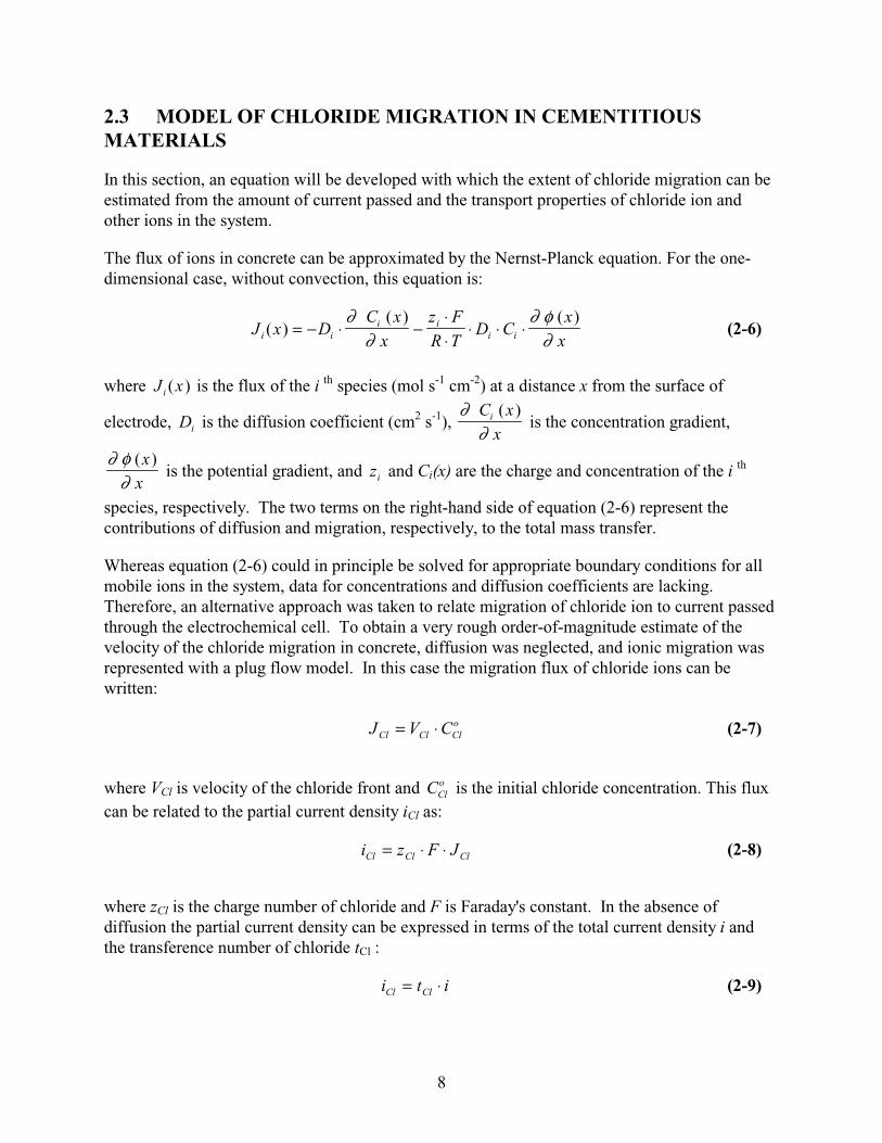
2.3 MODEL OF CHLORIDE MIGRATION IN CEMENTITIOUS MATERIALS

In this section, an equation will be developed with which the extent of chloride migration can be estimated from the amount of current passed and the transport properties of chloride ion and other ions in the system.

The flux of ions in concrete can be approximated by the Nernst-Planck equation. For the one-dimensional case, without convection, this equation is:

i ( ) = − Di ⋅ ∂ i

x

( ) −

z F ⋅ D Ci ⋅

∂ φ ( x) (2-6)J x

∂ C x i ⋅ i ⋅ R T ∂ x⋅

where J xi ( ) is the flux of the i th species (mol s-1 cm-2) at a distance x from the surface of ∂ C x

is the diffusion coefficient (cm2 s-1), ∂

i

x ( )

is the concentration gradient,electrode, Di

x∂ φ ( ) is the potential gradient, and zi and Ci(x) are the charge and concentration of the i th

∂ x

species, respectively. The two terms on the right-hand side of equation (2-6) represent the contributions of diffusion and migration, respectively, to the total mass transfer.

Whereas equation (2-6) could in principle be solved for appropriate boundary conditions for all mobile ions in the system, data for concentrations and diffusion coefficients are lacking. Therefore, an alternative approach was taken to relate migration of chloride ion to current passed through the electrochemical cell. To obtain a very rough order-of-magnitude estimate of the velocity of the chloride migration in concrete, diffusion was neglected, and ionic migration was represented with a plug flow model. In this case the migration flux of chloride ions can be written:

oJCl = VCl ⋅ CCl (2-7)

owhere VCl is velocity of the chloride front and CCl

can be related to the partial current density iCl as: is the initial chloride concentration. This flux

iCl = zCl ⋅ F ⋅ JCl (2-8)

where zCl is the charge number of chloride and F is Faraday's constant. In the absence of diffusion the partial current density can be expressed in terms of the total current density i and the transference number of chloride tCl :

iCl = tCl ⋅ i (2-9)

8

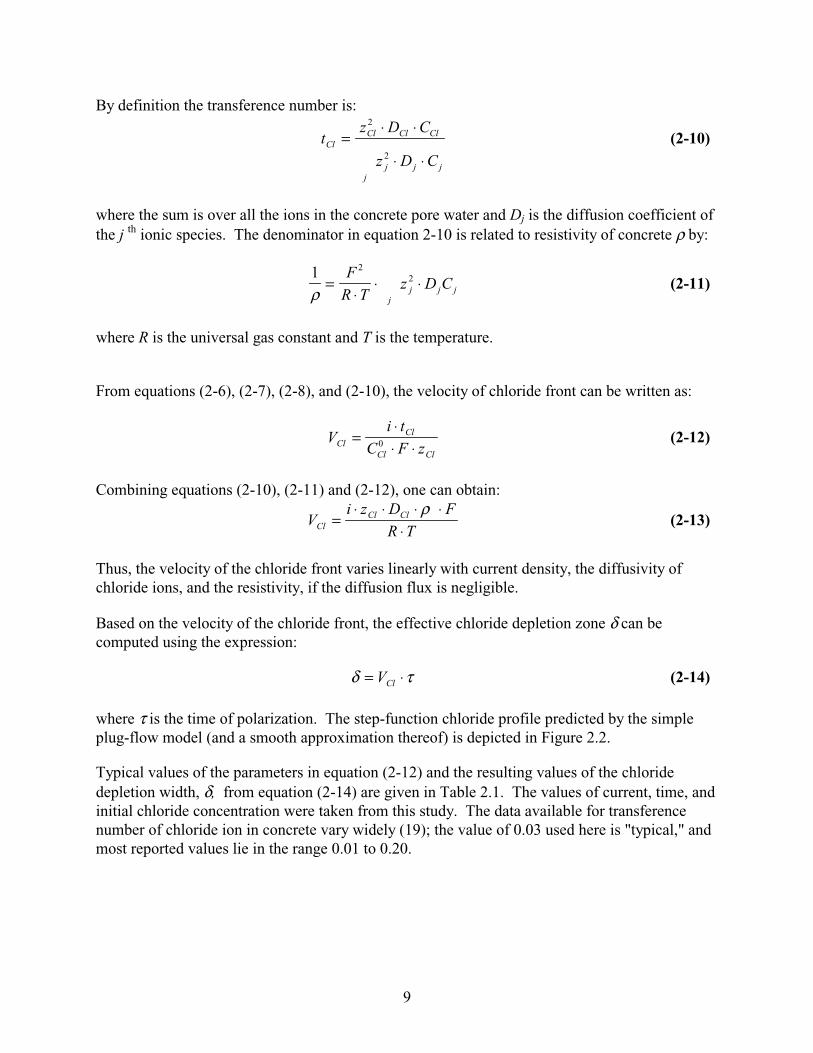
By definition the transference number is: 2zCl ⋅ DCl ⋅ CCltCl = (2-10)

2z D ⋅ Cj ⋅ j j j

where the sum is over all the ions in the concrete pore water and Dj is the diffusion coefficient of the j th ionic species. The denominator in equation 2-10 is related to resistivity of concrete ρ by:

1 F 2 2

ρ R T jj ⋅ j j (2-11)= ⋅ z D C

⋅

where R is the universal gas constant and T is the temperature.

From equations (2-6), (2-7), (2-8), and (2-10), the velocity of chloride front can be written as:

i t⋅ VCl = 0

Cl (2-12)FCCl ⋅ ⋅ zCl

Combining equations (2-10), (2-11) and (2-12), one can obtain: i zCl ⋅ DCl ⋅ ρ ⋅ F⋅

VCl = R ⋅ T

(2-13)

Thus, the velocity of the chloride front varies linearly with current density, the diffusivity of chloride ions, and the resistivity, if the diffusion flux is negligible.

Based on the velocity of the chloride front, the effective chloride depletion zone δ can be computed using the expression:

δ = VCl ⋅τ (2-14)

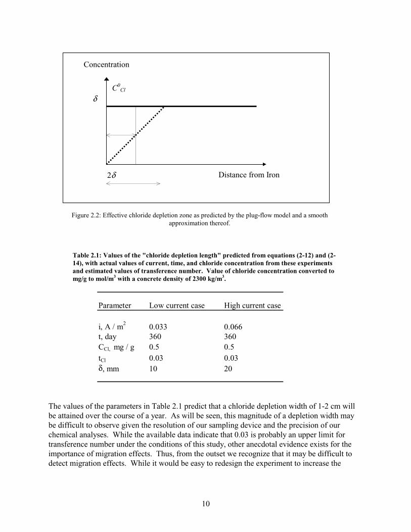
where τ is the time of polarization. The step-function chloride profile predicted by the simple plug-flow model (and a smooth approximation thereof) is depicted in Figure 2.2.

Typical values of the parameters in equation (2-12) and the resulting values of the chloride depletion width, δ, from equation (2-14) are given in Table 2.1. The values of current, time, and initial chloride concentration were taken from this study. The data available for transference number of chloride ion in concrete vary widely (19); the value of 0.03 used here is "typical," and most reported values lie in the range 0.01 to 0.20.

9

Concentration

Distance from Iron

δ

2δ

C0 Cl

Figure 2.2: Effective chloride depletion zone as predicted by the plug-flow model and a smooth approximation thereof.

Table 2.1: Values of the "chloride depletion length" predicted from equations (2-12) and (2-14), with actual values of current, time, and chloride concentration from these experiments and estimated values of transference number. Value of chloride concentration converted to mg/g to mol/m3 with a concrete density of 2300 kg/m3.

Parameter Low current case High current case

i, A / m 0.033 0.066 t, day 360 360 CCl, mg / g 0.5 0.5 tCl 0.03 0.03 δ, mm 10 20

2

The values of the parameters in Table 2.1 predict that a chloride depletion width of 1-2 cm will be attained over the course of a year. As will be seen, this magnitude of a depletion width may be difficult to observe given the resolution of our sampling device and the precision of our chemical analyses. While the available data indicate that 0.03 is probably an upper limit for transference number under the conditions of this study, other anecdotal evidence exists for the importance of migration effects. Thus, from the outset we recognize that it may be difficult to detect migration effects. While it would be easy to redesign the experiment to increase the

10

chances of observing a migration effect, the goal of the study is to test whether migration effects can be observed under these conditions.

Thus, the conclusions of this modeling exercise are: (i) the value for the transport number of Cl­

in concrete is a major source of uncertainty; (ii) in general it may be difficult to observe Cl­

migration by bulk analysis of concrete at current densities relevant for conventional or "accelerated" cathodic protection (2 - 100 mA/m2) within the time frame of a year (however, there is still considerable uncertainty in the values used for transport number -- use of alternative values for transport numbers could lead to other conclusions); and (iii) additional methods to monitor effects of migration (e.g., corrosion potential, corrosion current) or chloride concentration (e.g., electron microprobe) are indicated.

To determine experimentally the "effective chloride depletion zone" the reinforced concrete (mortar) system was polarized for one year. The experimental approach included preparation of the test blocks with known initial chloride concentration, application of long-term cathodic polarization, and determination of chloride concentration as a function of distance from the iron plate several times during the course of polarization.

11

3.0 ELECTROCHEMICAL EXPERIMENTS

This chapter is devoted to the electrochemical part of the project. First, we describe preparation of the test blocks, the objects of our study, then we continue with the preliminary electrochemical tests that were necessary for the subsequent long-term migration experiment.

3.1 PREPARATION OF TEST BLOCKS

Mortar was chosen as the material for the test blocks, since this type of concrete suits the purposes of the project better than other kinds of cementitious materials described earlier (see Section 2.2). Indeed, mortar has low shrinkage and possesses greater homogeneity, because only sand is used as an aggregate in its fabrication. From the greater homogeneity we benefit in the reduction of noise in the measured chloride profiles and easier mechanical sampling (drilling) of the blocks. In addition, a higher uniformity in the electrical field, ion migration, and diffusion are achieved if a fine aggregate is utilized. Finally, the bleeding effect is readily controlled when sand is the aggregate.

Bleeding was a concern in this project for the following reason. As a part of block fabrication, a known quantity of sodium chloride was introduced into the cement mixture to be cured. Bleed water will extract sodium chloride from the cement mixture and transport it to the top surface, causing an undesirable disturbance of initial chloride profile in the blocks. The way to avoid this problem is to use low water to cement ratio (see Section 2.2.2). Usage of low water to cement ratio has an additional advantage: higher strength of material, with the goal to have test blocks that are not subject to crumbling under the shock of the hammer drill used for sampling. The actual values of the water to cement ratios that we used were 0.35 and 0.5 (w/w).

Now let us consider two possible ways to introduce the chloride into the test blocks. One of them is natural diffusion of chloride ions into cement paste through the block surfaces; the other one is addition of chloride solution into the cement paste as the blocks are cast.

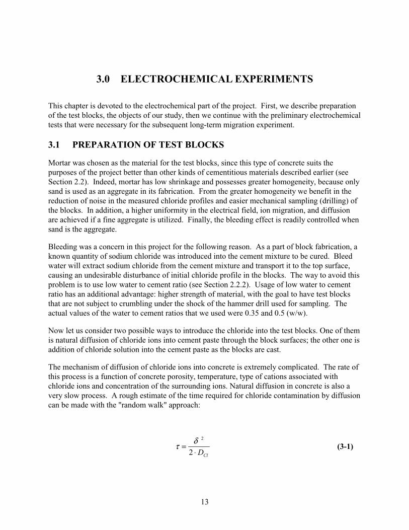
The mechanism of diffusion of chloride ions into concrete is extremely complicated. The rate of this process is a function of concrete porosity, temperature, type of cations associated with chloride ions and concentration of the surrounding ions. Natural diffusion in concrete is also a very slow process. A rough estimate of the time required for chloride contamination by diffusion can be made with the "random walk" approach:

2δτ = 2 ⋅ DCl

(3-1)

13

where δ is the average distance ions moved from the surface due to diffusion and DCl is the chloride diffusion coefficient, 2 Ù10-7 cm2/s (20). For the test blocks with dimensions 15 x 15 x 17 cm, the time required for chloride ions to penetrated "from wall to wall" is several years! Therefore introduction of chloride ions was accomplished by addition of sodium chloride to the cement-sand mixture during fabrication of blocks.

The steel mesh cathode, simulating the rebar, was embedded in the mortar blocks in the course of their fabrication. Zinc was chosen as the anode material because of its good adhesion to concrete and low cost. Two methods can be used to spray zinc onto the concrete surface: flame-spray or arc-spray. The latter method was used based on the availability of the equipment. Before metallization, the concrete surface was sandblasted to enhance the adhesion of zinc.

Portland cement was used for preparation of the mortar, since it is a typical component in actual reinforced concrete structures in Oregon. The mortar recipe was taken from standards (21) and the preparation procedure complies with standards of Oregon Department of Transportation (ODOT). Mortar blocks (15.2×15.2×17.8 cm) with embedded steel mesh were prepared in the ODOT facility. The characteristics of the blocks are summarized in Table 3.1.

Blocks 4A and 4B were polarized in several pilot tests (Section 3.2), preceding the long-term migration experiment (Section 3.3), in which blocks 1A, 1B, 2A, 2B, 3A, 3B, 4C and 4D were used. No polarization was applied to blocks 1D, 2D, 3D, 4E; hereafter these blocks are referred to as control blocks. Two other blocks, block 7 and the mortar blank block, were cast several months later according to the same standards, but no electrodes were introduced. These two blocks were used in determination of the reproducibility and accuracy of chloride analysis.

14

Table 3.1: Composition of mortar blocks. Values specific for block 7 are denoted with * if different from those for the rest for the blocks.

Identification of blocks 1A, 1B, 1D 2A, 2B, 2D

Nominal chloride concentration in: mg / g 0.39 0.78

lb / yd3 1.47 2.92 Water to cement ratio (w/w) 0.50 0.50

Cement (kg) 11.15 11.15 Water (L) 5.57 5.57 Sand (kg) 28.13 28.13

Mass of (C+W+S) mixture (kg) 44.85 44.85

Mass of mixture accounting for 4.5 % loss (kg) 42.83 42.83

Mass of NaCl added to the mixture (g) 27.80 55.35

Identification of blocks 3A, 3B, 3D 4A, 4B, 4C, 4D, 4E, 7*

Nominal chloride concentration in: mg / g 0.81 1.95 (1.45)*

lb / yd3 2.92 7.27 Water to cement ratio (w/w) 0.35 0.50

Cement (kg) 11.15 13.93 Water (L) 3.90 6.97 Sand (kg) 28.13 35.17

Mass of (C+W+S) mixture (kg) 43.18 56.07 Mass of mixture accounting for 4.5 % loss (kg) 41.24 53.54 Mass of NaCl added to the mixture (g) 55.35 172.9 (128.6)*

3.2 CATHODIC PROTECTION PILOT TESTS

The migration of ionic species in a porous solid under a small electric field is a slow process. Therefore, to investigate chloride ion migration in mortar, long-term polarization of mortar blocks is necessary. However, as shown by Cramer and coworkers (22), a very high driving voltage is required to maintain constant current in the course of such experiments. They concluded that this change in voltage was a result of electrochemical reactions occurring at the zinc-concrete interface when it was polarized. It was shown that changes in effective resistance at the anode/concrete interface were induced by the formation of oxidation products such as zinc oxide, zinc hydroxide, zinc sulfate and zinc chloride. The conductivity of the system is also affected by the amount of water present in the pore structure of the cementitious material. Investigation of reinforced concrete structures set under potentiostatic cathodic protection

15

conducted by Oregon and California Departments of Transportation showed that the currents through these systems were higher during the wet winter season and lower during the dry summer time (23). Therefore, before the long-term migration experiment, a series of preliminary tests were conducted to investigate these issues (24, 23).

3.2.1 Types of Cathodic Protection

Cathodic protection in concrete systems can be applied either potentiostatically (controlled-potential) or galvanostatically (controlled-current) in both two- and three-electrode configurations.

Under potentiostatic control, the potential of the steel cathode is to be maintained constant. In a two-electrode system, a known voltage is applied across the steel cathode and the zinc anode. The zinc anode both completes the circuit, allowing charge to flow through the system, and serves as a de facto reference for measurement of cathode potential. However, the zinc-concrete interface is subject to polarization, often resulting in an unknown and variable voltage drop at that interface. In a three-electrode system, the potential of the steel cathode is maintained constant relative to an additional reference electrode, which is placed close to the steel cathode. The reference electrode does not pass the current and therefore its potential is stable under polarization.

Under galvanostatic control, the current flowing between the steel mesh and the sprayed zinc electrode is fixed. In this mode the precise control of the applied current can be accomplished with a two-electrode configuration. However, if it is desired to measure the potential of the steel cathode as a function of time, and the anode is polarizable, a three-electrode arrangement is used.

To provide reliable cathodic protection, the current through the system should be sufficiently high to stop corrosion. On the other hand, exceedingly high current would cause significant disturbance of the protected system (e.g., evolution of hydrogen). Therefore, part of the design of the cathodic protection system is the selection of the appropriate current density for galvanostatic protection or the appropriate potential of steel for potentiostatic protection. ODOT, based on years of practical experience, has found that values of 0.0022 A/m2 are suitable for protection of coastal concrete structures in Oregon (24). In the case of potentiostatic mode of protection the optimum applied voltage is about 3 V (25).

3.2.2 Potentiostatic Experiment

First a pilot test was performed in the two-electrode potentiostatic mode. Two mortar blocks of the same composition, blocks 4A and 4B (see Table 3.1), were placed in a chamber with temperature 25 0C and relative humidity about 85 %. To prevent the loss of moisture from the zinc side of block 4A, this side of the block was covered with saran wrap and a cast iron heat sink was placed on top of it. The heat sink helped to dissipate heat developed during polarization. Such a measure was supposed to prevent moisture loss and increase in the resistance at the zinc-concrete interface. The second block, block 4B, was left unwrapped for comparison. An EG & G Princeton Applied Research Potentiostat / Galvanostat Model 273A and Model 173 were used in a two-electrode potentiostat mode to apply -1 V (Fe vs. Zn) to each

16

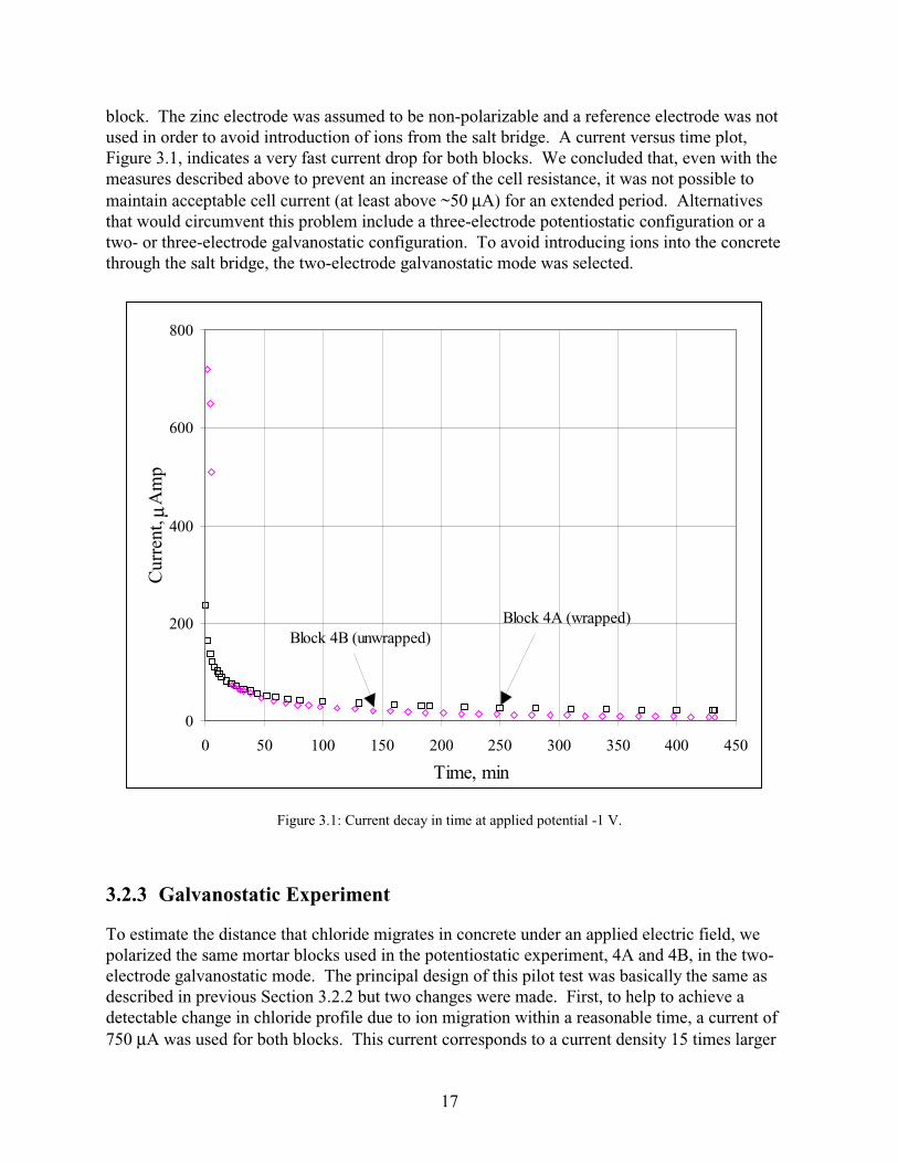
block. The zinc electrode was assumed to be non-polarizable and a reference electrode was not used in order to avoid introduction of ions from the salt bridge. A current versus time plot, Figure 3.1, indicates a very fast current drop for both blocks. We concluded that, even with the measures described above to prevent an increase of the cell resistance, it was not possible to maintain acceptable cell current (at least above ~50 µA) for an extended period. Alternatives that would circumvent this problem include a three-electrode potentiostatic configuration or a two- or three-electrode galvanostatic configuration. To avoid introducing ions into the concrete through the salt bridge, the two-electrode galvanostatic mode was selected.

0

200

400

600

800

0 50 100 150 200 250 300 350 400 450

Time, min

Cur

rent

, =µA

mp

Block 4A (wrapped) Block 4B (unwrapped)

Figure 3.1: Current decay in time at applied potential -1 V.

3.2.3 Galvanostatic Experiment

To estimate the distance that chloride migrates in concrete under an applied electric field, we polarized the same mortar blocks used in the potentiostatic experiment, 4A and 4B, in the two-electrode galvanostatic mode. The principal design of this pilot test was basically the same as described in previous Section 3.2.2 but two changes were made. First, to help to achieve a detectable change in chloride profile due to ion migration within a reasonable time, a current of 750 µA was used for both blocks. This current corresponds to a current density 15 times larger

17

than the typical value of 0.0022 A/m2 employed by ODOT in coastal cathodic protection systems (24). The current and the driving voltage across each block were recorded at 15 minute intervals with an automated data acquisition system. Second, the unwrapped block 4B was sprayed with distilled water whenever the absolute value of the driving voltage (i.e. potential of steel cathode vs. zinc anode) reached -10 V.

After ~ 40 days of polarization both blocks were sampled along the line perpendicular to the steel mesh and analyzed for chloride. For more details of sample preparation and chloride analysis, see Section 4.4.

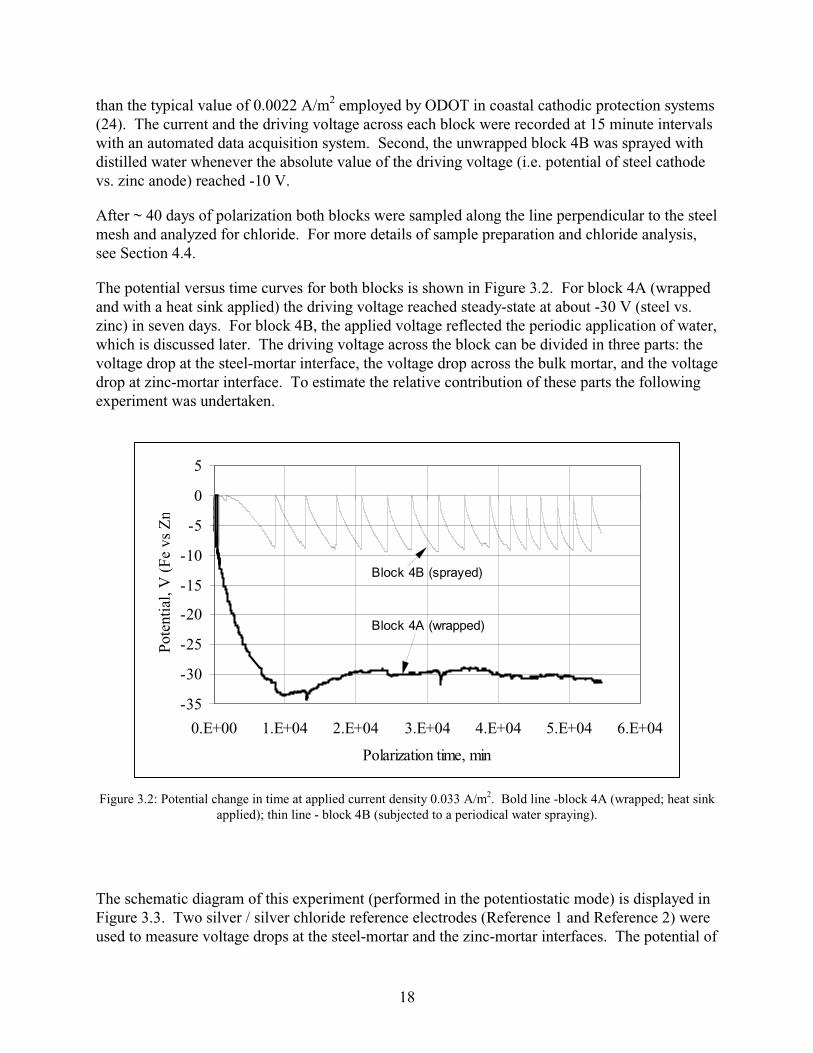
The potential versus time curves for both blocks is shown in Figure 3.2. For block 4A (wrapped and with a heat sink applied) the driving voltage reached steady-state at about -30 V (steel vs. zinc) in seven days. For block 4B, the applied voltage reflected the periodic application of water, which is discussed later. The driving voltage across the block can be divided in three parts: the voltage drop at the steel-mortar interface, the voltage drop across the bulk mortar, and the voltage drop at zinc-mortar interface. To estimate the relative contribution of these parts the following experiment was undertaken.

-35

-30

-25

-20

-15

-10

-5

0

5

0.E+00 1.E+04 2.E+04 3.E+04 4.E+04 5.E+04 6.E+04

Polarization time, min

Pote

ntia

l, V

(Fe

vs

Zn

Block 4A (wrapped)

Block 4B (sprayed)

Figure 3.2: Potential change in time at applied current density 0.033 A/m2. Bold line -block 4A (wrapped; heat sink applied); thin line - block 4B (subjected to a periodical water spraying).

The schematic diagram of this experiment (performed in the potentiostatic mode) is displayed in Figure 3.3. Two silver / silver chloride reference electrodes (Reference 1 and Reference 2) were used to measure voltage drops at the steel-mortar and the zinc-mortar interfaces. The potential of

18

the steel cathode relative to Reference 1 (i.e., voltage drop at steel-mortar interface) was maintained constant at -1V . Results of these measurements are presented in Figure 3.4. They indicate that the largest potential drop occurs at the zinc-mortar interface. This build up of resistance has been attributed to the formation of zinc oxidation products (26).

M o rtar b loc k

E F e v s Z n ( by D V M )

E Z n v s R ef 2

E F e v s R e f 1

A g /A g C l

(se t valu e )

( by D V M )

Iro n Z in c .

Figure 3.3: Determination of the voltage drop across the block.

Now let us return back to discussion of galvanostatic experiment. The behavior of block 4B was different from that of block 4A. Results for 4B confirmed that the effect of water on the potential is important. As Figure 3.2 indicates, the potential changed in the saw pattern during polarization, with each spike corresponding to the application of water. Initially the value of the driving voltage went up to -10 V. Spraying of the block with distilled water induced a fast reduction in the absolute value of the driving voltage. If the assumption about the formation of the barrier layer from zinc oxidation products is valid, then the role of water can be explained as follows. Distilled water, applied to the zinc surface, penetrates the mortar and dissolves or

19

hydrates part of the oxidation products. As we saw earlier in this section, the resistance of the zinc-mortar interface is a major contributor to the total resistance of the block; therefore the voltage drop across the system (i.e. driving voltage) is approximately proportional to the zinc-mortar resistance. Over the course of polarization, the time period for the driving voltage to reach the -10 V limit noticeably decreases, as shown in Figure 3.2. This observation suggests that water only partially "destroys" the barrier layer formed at the zinc-mortar interface and its thickness increases with time.

-10

0

10

20

30

40

0 8 12 16

Distance from Steel, cm

Pote

ntia

l Dro

p, V

4

Figure 3.4: Potential drop across mortar block at Esteel = -1 V vs. silver / silver chloride electrode.

Results of the galvanostatic experiment, described in this section, show that application of water during cathodic protection allows us to maintain the necessary current density while keeping the driving voltage within practically reasonable limits. For this reason the method was selected for the long-term migration experiment.

3.3 LONG-TERM MIGRATION EXPERIMENT

The long-term migration experiment was performed with eight blocks (see Section 3.3.2 for details) to investigate the migration of chloride ions from the steel electrode towards the zinc-mortar interface. over the course of one year. The blocks were divided into two groups based on their initial compositions and the currents applied to them. The steel vs. zinc potential was recorded every 15 minutes over the whole period. To monitor the change in the concentration of chloride ions in the blocks, all blocks were sampled four times during the one-year polarization.

20

Chloride analysis of the mortar samples was accomplished by ion chromatography and is discussed in Chapter 5.0 of this thesis.

3.3.1 Power Supply and Data Logger

A power supply provided constant current to eight test blocks and sent signals corresponding to the applied current and applied voltage to a data logger. A schematic diagram of the power supply is given in Figure 3.5. This device maintains constant current through a load (mortar block) in the course of polarization. The line voltage of 120 VAC is reduced by transformers T1 and T2 to an output of 72 VAC. Rectifier W06M is responsible for the conversion of AC voltage to DC. Capacitor C1 (3600 µF) filters out voltage fluctuations after rectification. The sequential chain of three 3.3 kohm resistors provides the discharge path for the capacitor C1 after power shutdown and is incorporated into the system for safety reasons. Two field effect transistors LND 150N3 serve as current stabilizers based on negative feedback. If the voltage experiences, say, a positive fluctuation, the voltage on the drain goes up as does the current. Since the gate is directly connected to the drain, this increase in drain voltage causes partial closure of the transistor (transistor's resistance goes up), which leads to the current decline. If there is a negative voltage deviation, it is reduced by the negative feedback in a similar way. In such a manner the current through the transistor is stabilized at a certain level.

T1

120 VAC

Power Source SP6231

+/-15 V, 200 mA

On

T2

COM

Power

Supply

For Buffer

Amps

3600 uF 150VDC

Power Indicator

~ 110 VDC 3.3 kOhm 1 W each

One Channel of Eight

Voltage across the load is (VM 10) - VC = VL

Current through the load is VC / 4000 = Iload

+

-

~

~ +

-

~ LND150N3

Ten Turn Pot 100 kOhm

Load

(VL)

Iload 0 to 2.5 mA

Current Sense Resistor

4 kOhm 1% 1/4 W Current

Monitor

(VC)

10 MOhm

51 Ohm

24 VAC

24 VAC

24 VAC

1.1 MOhm

200 kOhm Trim Pot

+ 15 V

100 nF

100 nF

1/4 LF347

- 15 V

10 Ohm 1/4 W

(VM)

10 Ohm 1/4 W

Voltage Monitor

W06M

C1

Figure 3.5: Schematic diagram of power supply.

A ten-turn potentiometer (100 kohm) allows one to adjust the current. Since the resistance of the load is much smaller than 100 kohm, and the change in the load resistance in the course of the experiment is even smaller, the influence on the overall resistance (and hence the load current) by such a variation is negligible. The voltage follower based on operational amplifier OA LF347

21

acts as a buffer between the system and the monitor to eliminate the load of the voltmeter or other measuring device on the power supply. The current sense resistor provides a way to monitor the current through the load (10 V per 2.5 mA of the load current). The output signals from each of eight channels of power supply VM and VC were recorded by the data logger, which consisted of a DAS1600 board, a personal computer, and a Visual Basic program DVM 16.

3.3.2 Layout of Experiment

In the long-term migration experiment the effect of two different current settings with four different initial compositions of mortar was studied. Eight blocks (1A, 1B, 2A, 2B, 3A, 3B, 4C, 4D) were subjected to different polarization conditions in the course of the experiment performed in the controlled environment room of the Albany Research Center of the U. S. Department of Energy.

These blocks were divided into two groups. The first group of blocks (1A, 2A, 3A, and 4C) were polarized at a current density of 0.066 A/m2, and the second group (1B, 2B, 3B, and 4D) was polarized at 0.033 A/m2. Blocks designated by the same number (e.g., 1A and 1B) were of the same composition (Table 3.1). Three pairs of blocks (1A, 1B; 2A, 2B; and 4C, 4D) were prepared with a water to cement ratio of 0.5 (w/w), and one pair (3A, 3B) with a water to cement ratio of 0.35 (w/w). Blocks 1A, 1B had low chloride (0.39 mg/g); blocks 2A, 2B and 3A, 3B had intermediate chloride (0.78 and 0.81 mg/g, respectively); and blocks 4C, 4D had high chloride (1.95 mg/g).

A diagram of the experiment is shown in Figure 3.6. To keep the voltage drop across the blocks below the power supply's upper limit (100 V), a pond with 500 mL of saturated calcium hydroxide solution was attached to the zinc side of each block in lieu of manual spraying with distilled water described in Section 3.2.3. The blocks were placed in the room with controlled temperature and humidity, about 25 0C and 75 - 85 %, respectively.

All eight blocks were sampled for chloride analysis four times during the experiment: before start of polarization, and after 2, 3.5, and 11 months of polarization. All mortar powder samples were digested in water and analyzed by ion chromatography. Details and results of the chloride analysis are given in Chapter 5.0.

22

Eight channels power supply

Iout PC with DAS-1600 board

Current monitor signal

Voltage monitor signal

Pond with saturated calcium hydroxide

Controlled humidity room

To sprayed zinc side

To iron mesh

Figure 3.6: Layout of long-term migration experiment. One block out of eight is shown.

3.3.3 Analysis of Potential Profiles

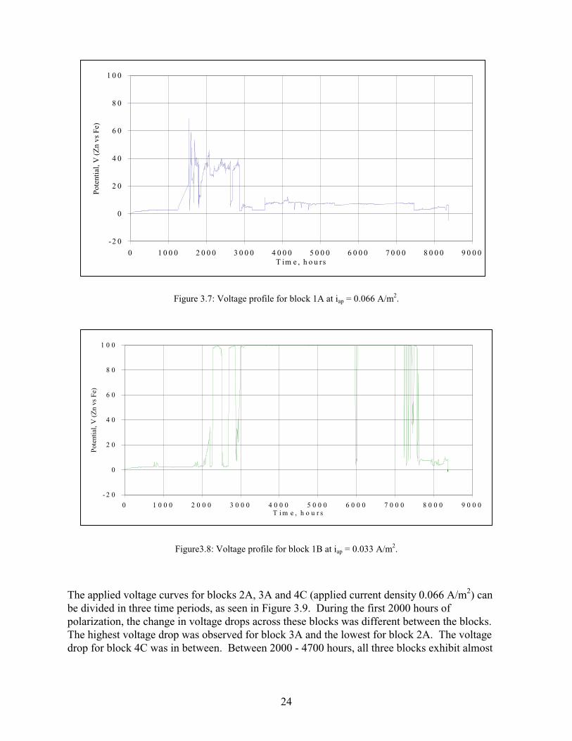
The applied voltage as a function of time for the two-electrode galvanostatic experiments are presented in Figure 3.7, Figure 3.8, Figure 3.9 and Figure 3.10. These data are replotted to allow comparisons of applied voltage versus time for the same block compositions but different current settings in Figure 3.11, Figure 3.12 and Figure 3.13.

Applied voltage versus time curves for blocks 1A and 1B exhibit sudden fluctuations of unknown origin and are not discussed any further in this section. Voltage drops developed across the six other blocks (2A, 2B, 3A, 3B, 4C and 4D) did not exceed 4 V. These drops are much lower than the voltage drop observed for the non-sprayed block 4A (~ 30 V) and match the voltage drop across the sprayed block 4B (below10 V), as described in Section 3.2.3. This result confirms that ponds with calcium hydroxide solution applied on top of the blocks indeed successfully replaced the manual water spraying.

23

-2 0

0

2 0

4 0

6 0

8 0

1 0 0

0 1 0 0 0 2 0 0 0 3 0 0 0 4 0 0 0 5 0 0 0 6 0 0 0 7 0 0 0 8 0 0 0 9 0 0 0 T i m e , h o u r s

Pote

ntia

l, V

(Z

n vs

Fe)

Figure 3.7: Voltage profile for block 1A at iap = 0.066 A/m 2 .

- 2 0

0

2 0

4 0

6 0

8 0

1 0 0

0 1 0 0 0 2 0 0 0 3 0 0 0 4 0 0 0 5 0 0 0 6 0 0 0 7 0 0 0 8 0 0 0 9 0 0 0 T i m e , h o u r s

Pote

ntia

l, V

(Z

n vs

Fe)

Figure3.8: Voltage profile for block 1B at iap = 0.033 A/m 2 .

The applied voltage curves for blocks 2A, 3A and 4C (applied current density 0.066 A/m2) can be divided in three time periods, as seen in Figure 3.9. the first 2000 hours of polarization, the change in voltage drops across these blocks was different between the blocks. The highest voltage drop was observed for block 3A and the lowest for block 2A. e drop for block 4C was in between. etween 2000 - 4700 hours, all three blocks exhibit almost

During

The voltagB

24

identical profiles. After 4700 hours of polarization the voltage curves separated from each other and merged together again after about 7200 hours of polarization.

-3

-2

-1

0

1

2

3

4

5

0 1 0 0 0 2 0 0 0 3 0 0 0 4 0 0 0 5 0 0 0 6 0 0 0 7 0 0 0 8 0 0 0 9 0 0 0 T im e , h o u rs

Pote

ntia

l, V

(Z

n vs

Fe)

B lo c k 4 C

B lo c k 3 A

B lo c k 2 A

Figure 3.9: Voltage profiles for blocks 2A, 3A and 4C at iap = 0.066 A /m 2 .

-3

-2

-1

0

1

2

3

4

5

0 1000 2000 3000 4000 5000 6000 7000 8000 9000 Tim e , hours

Pote

ntia

l, V

(Z

n vs

Fe)

B lock 4D

B loc k 3B

B lock 2B

Figure 3.10: Voltage profiles for blocks 2B, 3B and 4D at iap = 0.033 A/m 2 .

25

-3

-2

-1

0

1

2

3

4

5

0 1000 2000 3000 4000 5000 6000 7000 8000 9000

T im e, h o u rs

Pote

ntia

l, V

(Z

n vs

Fe)

Blo ck 2B ( I= 0.75 m A )

B lock 2A (I=1 .5 m A )

Figure 3.11: Comparison of potential profiles of blocks 2A and 2B.

-3

-2

-1

0

1

2

3

4

5

0 1000 2000 3000 4000 5000 6000 7000 8000 9000

T im e, hour s

Pote

ntia

l, V

(Z

n vs

Fe)

Block 3B (I= 0.75 m A )

Block 3A (I = 1.5 m A )

Figure 3.12: Comparison of potential profiles of blocks 3A and 3B.

26

-3

-2

-1

0

1

2

3

4

5

0 1000 2000 3000 4000 5000 6000 7000 8000 9000 Time, hours

Pot

entia

l, V

(Z

n vs

Fe)

Bloc

Bloc

Block 4D (I=0.75 mA)

Block 4C (I=1.5 mA)

.

Figure 3.13: Comparison of potential profiles of blocks 4C and 4D.

Voltage curves for blocks 2B, 3B and 4D (applied current density 0.033 A/m2) can be divided in two time periods. Within the first 4000 hours of polarization, the voltage drops were different in these blocks as shown in Figure 3.10. The highest among them was voltage drop across block 3B. The lowest voltage drop occurred in block 2B. The curve for block 4D lies between the other two. The second period starts after 4000 hours. During this period three curves converge and stay together until the end of polarization.

Voltage curves are quite similar for the blocks of similar composition at different current densities, particularly for blocks 4C (current density 0.066 A/m2) and 4D (current density 0.033 A/m2), as shown in Figure 3.13. The curve of block 3A (current density 0.066 A/m2) lies slightly below the curve for 3B (current density 0.033 A/m2) (Figure 3.12). The relationship between voltage curves for blocks 2A and 2B has a different pattern. During first 4000 hours of polarization curve 2A (current density 0.066 A/m2) is above curve 2B (current density 0.033 A/m2). At the time point of 4000 hours the two curves cross and their relative positions interchange, as shown in Figure 3.11.

At constant current, the voltage drop across each block is defined by the effective resistance of the block. In the bulk of mortar the electric current is conducted essentially by free ions in the capillary water. Resistance of the bulk mortar should decrease with increase of the water to cement ratio and the concentration of free ions in mortar. The effect of water was observed during the first period of polarization at both current conditions (0.033 and 0.066 A/m2). For example, during the first 2000 hours of polarization the voltage drop across block 3A (w/c=0.35)

27

was higher than that for blocks 2A and 4C (w/c = 0.5). However, no effect of initial chloride concentration on the voltage drop was observed in this case: block 4C with higher chloride content exhibited the voltage drop higher than that of block 2A, just the opposite to what was expected.

In summary, expectations based on initial w/c content and initial chloride content were not observable, and no satisfactory explanation for the observations exists.

28

4.0 CHLORIDE ANALYSIS BY POTENTIOMETRIC METHODS

4.1 REVIEW OF METHODS FOR DETERMINATION OF CHLORIDE IN CONCRETE

The most common methods used to determine the concentration of chloride ion in concrete include visible spectrophotometry, atomic absorption spectrophotometry, neutron activation analysis, potentiometric titration, and potentiometry by standard additions. Another technique is ion chromatography.

The classical method for the determination of the chloride content of concrete requires pulverization of concrete, digestion of the concrete powder and potentiometric titration of the resulting aqueous sample (27). This technique is arduous, time-consuming and expensive. Since the 1960s many alternative methods have been developed.

In the spectrophotometric method, samples are pulverized and digested in acid. The resulting aqueous extract is treated with mercuric thiocyanate and ferric ion solution. The absorbance of the resulting pentaaquothiocyanatoiron(III) chloride complex, [Fe(OH2)5 SCN]Cl2 is then measured. This technique is very sensitive to interference at low pH values (27).

The atomic absorption procedure is based on pulverization, extraction, and precipitation of the chloride in a sample solution by the addition of a known and excess amount of silver ion. Then, the amount of either the unreacted silver or the precipitated silver is determined by atomic absorption spectrophotometry. This method requires that the matrix of the standard solutions be matched to that of the sample solutions in order to eliminate the matrix effect (28).

Neutron activation analysis is another technique for chloride analysis of concrete. In this analysis the sample is bombarded with neutrons to transform the natural isotope 37Cl to 38Cl, which emits gamma rays in direct proportion to the amount of its precursor isotope. By comparison of the radioactivities of the sample and a standard irradiated under identical conditions, the chloride content of the sample can be determined. The presence of radioisotopes such as 24Na, 27Mg, 28Al, 42K, 51Ti and 56Mn contribute to high backgrounds that make chloride determination difficult (28).

In the potentiometric titration procedure, an aqueous extract of the digested concrete is titrated with a standardized AgNO3 solution to form solid AgCl(s). The equivalence point is determined with a chloride ion-selective electrode and reference electrode (27).

In potentiometry with standard additions, to a known volume of extract from the pulverized and digested concrete samples, two additions of a standard chloride solution are made. The potential difference between a chloride ion-selective electrode and a reference electrode is measured after

29

each addition. The response slope of the electrode is determined by repetitive spiking of a matrix blank solution with the same standard chloride solution.

Ion chromatographic determination of chloride is based upon ion-exchange separation of chloride from other anions in the matrix and coductivity detection. A quaternary ammonium group in the hydroxide form (-NR3OH) provides the anion exchange sites. The calibration slope is simply obtained by injecting standard solutions with known chloride concentration and correlating the peak-height or peak-area response from a conductivity detector with concentration.

In this work the following methods were considered for analysis of mortar for chloride: potentiometric titration, potentiometry by standard additions, and ion chromatography (IC). Section 4.2 of this chapter deals with a method of digestion of mortar and extraction of chloride. In Section 4.3, potentiometric titration curves for various chloride concentrations are shown to illustrate why the classical method, potentiometric titration, could not be used in this project. Section 4.4 is devoted to the analysis of mortar for chloride by direct potentiometry with standard additions. Consideration of the determination of chloride by IC is given in Chapter 5.0.

4.2 SOME ASPECTS OF CHLORIDE DIGESTION

The chloride in concrete can be considered to be chemically bound (incorporated in solids), physically bound (adsorbed), or free in aqueous pore solution (29). It is thought that only free chloride is significant in the corrosion process. Extraction of pulverized concrete with nitric acid is said to yield total chloride (both free and bound). Extraction with water is generally said to yield the free chloride, although the extent of extraction depends on several factors such as the nature of the sample, temperature, and the duration of the extraction step. Water soluble chloride values are often about 85 % of the acid soluble values (30). One of the problems associated with extraction of chloride from mortar by either water or acid is variable efficiency.

In the initial phase of this study, samples were prepared by acid extraction and analyzed by double standard addition ion-selective electrode potentiometry. However, as will be discussed, better precision was obtained with water extraction and ion chromatography, which was used for the bulk of the study.

4.3 POTENTIOMETRIC TITRATION

As mentioned earlier, potentiometric titrations are widely used to determine the chloride content of mortar (concrete) samples. In this procedure, a powdered concrete sample is digested with nitric acid to extract chloride. The chloride is then titrated with a standardized AgNO3 solution to form an AgCl(s) precipitate. This chemical reaction is represented as

Cl − + Ag + = AgCls (4-1)

By measuring the electrical potential between a chloride ion-selective electrode and a reference electrode as the titration progresses, one can determine the equivalence point and, subsequently, the chloride content.

30

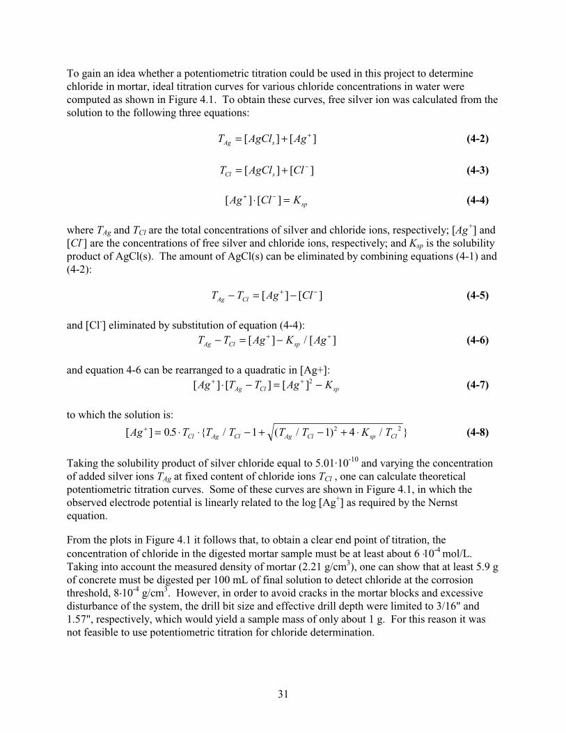
To gain an idea whether a potentiometric titration could be used in this project to determine chloride in mortar, ideal titration curves for various chloride concentrations in water were computed as shown in Figure 4.1. To obtain these curves, free silver ion was calculated from the solution to the following three equations:

+TAg = [ AgCls ] + [ Ag ] (4-2)

TCl = [ AgCls ] + [Cl − ] (4-3)

[ Ag + ] ⋅ [Cl − ] = Ksp (4-4)

where TAg and TCl are the total concentrations of silver and chloride ions, respectively; [Ag+] and [Cl-] are the concentrations of free silver and chloride ions, respectively; and Ksp is the solubility product of AgCl(s). The amount of AgCl(s) can be eliminated by combining equations (4-1) and (4-2):

TAg − TCl = [ Ag + ] − [Cl − ] (4-5)

and [Cl-] eliminated by substitution of equation (4-4): TAg − TCl = [ Ag + ] − Ksp / [ Ag + ] (4-6)

and equation 4-6 can be rearranged to a quadratic in [Ag+]: [ Ag + ] ⋅ [TAg − TCl ] = [ Ag + ]2 − Ksp (4-7)

to which the solution is: + .[ Ag ] = 0 5 ⋅ TCl ⋅{TAg / TCl − 1 + ( / ) / } T T K TAg Cl sp Cl − + ⋅ 1 4 2 2 (4-8)

Taking the solubility product of silver chloride equal to 5.01·10-10 and varying the concentration of added silver ions TAg at fixed content of chloride ions TCl , one can calculate theoretical potentiometric titration curves. Some of these curves are shown in Figure 4.1, in which the observed electrode potential is linearly related to the log [Ag+] as required by the Nernst equation.

From the plots in Figure 4.1 it follows that, to obtain a clear end point of titration, the concentration of chloride in the digested mortar sample must be at least about 6 ⋅10-4 mol/L. Taking into account the measured density of mortar (2.21 g/cm3), one can show that at least 5.9 g of concrete must be digested per 100 mL of final solution to detect chloride at the corrosion threshold, 8Ù10-4 g/cm3. However, in order to avoid cracks in the mortar blocks and excessive disturbance of the system, the drill bit size and effective drill depth were limited to 3/16" and 1.57", respectively, which would yield a sample mass of only about 1 g. For this reason it was not feasible to use potentiometric titration for chloride determination.

31

-7.0

-6.0

-5.0

-4.0

-3.0

-2.0

0.0 0.5 1.0 1.5 2.0 TAg/TCl

log[

Ag]

8⋅10-4 molCl/ L

6⋅10-4 molCl / L

2⋅10-4 molCl / L

4⋅10-4 molCl / L

Figure 4.1: Potentiometric titration of Cl- with Ag+. Theoretical curves.

4.4 POTENTIOMETRY BY STANDARD ADDITIONS

The determination of chloride in concrete by standard additions with chloride ion-selective electrode potentiometry has been used since 1970 (27). This experimental technique is relatively simple. The potential between the chloride ion-selective electrode and the reference electrode is measured initially and after two standard additions. Double standard additions permits more precise determination of low concentrations of chloride ions compared to single standard additions.

The following equations were used in our calculations of the unknown chloride concentration. The Nernst equations for the 1st and 2nd standard additions are given by:

E1 = E0 − S ⋅ log(Cx + ∆C1 ) (4-9)

E2 = E0 − S ⋅ log(Cx + ∆C2 ) (4-10)

32

where E1, E2 are potentials (V) after the 1st and 2nd standard additions, respectively; E0 denotes the formal potential (V); S is the response slope (V/decade) obtained from the calibration data; Cx represents unknown chloride concentration (mol/L); ∆C1 and ∆C2 are the 1st and 2nd additions (mol/L). The following equation was used for calculation of ∆C1 and ∆C2 :

∆C Cstd ⋅Vad / (Vc + Vad ) (4-11)=

where Cstd is the concentration of standard chloride solution, (mol/L); Vad and Vc are volume of addition and the initial volume of the sample solution in the cell (L), respectively. The two equations (4-9) and(4-10) are solved for the unknown concentration Cx :

∆C2 − ∆C1 ⋅ A Cx =

A − 1 (4-12)

where E E21 −

A = 10 S (4-13)

Thus, the experimental data required to calculate analyte concentration are E1, E2, ∆C1 , ∆C1 and S.

4.4.1 Instrumentation and Materials

Sodium chloride (Mallinckrodt AR, 99.8 %) was used to prepare a 1001 mgCl/L standard solution for additions and calibration. A 1.00 M supporting electrolyte was prepared from sodium nitrate (Mallinckrodt AR, 99.8 %). Diluted nitric acid solution for digestion of chloride from mortar was made from Baker Analyzed (for Trace Metal Analysis, 70.5 %) reagent. Orion Inner Reference Solution #90-00-02 was used to fill the inner sleeve of the reference silver/silver chloride electrode. Orion Outer Sleeve Solution (10 % potassium nitrate, w/w) was used to fill the outer sleeve. Deionized water (DI) was generated from a Millipore Milli-Q system.

Samples of concrete powder were weighed on a Mettler AE240 analytical balance (resolution 0.0001 g). Additions of standard sodium chloride solution were performed with a Metrohm Model 665 automicroburette. A magnetic stirrer was used to stir the solution in the cell. The cell potential (Orion Model 94-17B chloride ion-selective electrode vs. Orion double junction reference electrode) was measured with an Orion Model 701A digital pH / mV meter with a resolution of 0.1 mV. A Neslab Model RTE- 8 DD refrigerated circulating bath was employed to maintain a constant temperature in the cell (25 C) during measurements.

4.4.2 Sample Handling and Processing

Samples of mortar powder for chloride analysis were obtained from the blocks with a concrete drill. Holes were nominally 3/16" in diameter by 1.57" deep. To collect mortar powder as the hole was being drilled, a small envelope folded from weighing paper was attached just below the hole. To avoid the problem of contamination of mortar powder the following precautions were taken. First, latex gloves were used during sampling. Second, the drill bit and mortar block

33

surface were cleaned with acetone before operation. Third, the first portion of mortar obtained from the top layer of about 0.5 cm was discarded.

The possibility that the latex gloves and weighing paper could be a source of chloride contamination was checked. An extract of two glove fingers (mass about 1 g) was prepared according to the sample preparation procedure given in Section 5.1.4 and analyzed for chloride by ion chromatography described later in Chapter 5.0. It was found that the average concentration of chloride ions in glove extract was 0.11 mg/L (relative standard deviation 0.74 %, N=3). The extract of one weighing paper (mass about 0.4 g) gave the average chloride content of 0.03 mg/L (relative standard deviation 3.71 %, N=3). These amounts of chloride are negligible compared to the working range of concentrations: 1-15 mg/L. Actual contamination from gloves and paper was even less, since during normal sample preparation neither gloves nor paper were boiled along with mortar powder. These results show that the latex gloves and weighing paper were appropriate materials to use for sample collection.

The acid extraction procedure for the sample digestion was based on the ASTM method (31) with some modifications. Sample size was decreased from 10 g down to 0.2 - 0.5 g; the digestion was carried out with 7.5 mL of water and 2.5 mL of diluted 1:1 nitric acid instead of 75 mL and 25 mL, respectively; and the sample was allowed to cool before dilution to volume with water. The sample digestion procedure included the following steps. First, about 0.2 - 0.5 g of mortar powder was weighed and transferred to a 50 mL beaker. Immediately thereafter, 7.5 mL of DI water and 2.5 mL of diluted 1:1 nitric acid (v/ v) were added, and the mixture was swirled to break up any clumps. Then 3 - 5 drops of methyl orange indicator were dispensed into the beaker. After two minutes dilute nitric acid was added dropwise, if necessary, until a faint pink color persisted. Afterwards, the solution was rapidly brought to 5 min boiling in a covered beaker. After the sample cooled to room temperature it was transferred to a 100 mL volumetric flask. The sides of the beaker and the sediment remaining in the beaker were washed several times with DI water, and this portion of the sample was combined with the solution in the volumetric flask. The sediment was allowed to settle to the bottom of the flask before measurements.

A similar procedure was used to prepare a digestion blank with the only difference in the first step: about 30 mL of DI water were placed into the beaker instead of mortar powder.

4.4.3 Analysis Procedure

All measurements were performed at constant temperature of 25 C. The automicroburette was set to a volume increment of 40 µL, and the concentration of the titrant was 1001 mg/L chloride. Before measurements the cell and the electrodes were rinsed with DI water several times. After that, the cell was vacuum dried and the remaining drops on the electrodes or microburette tip were blotted with a tissue. Next, 25 mL of digestion blank was added to the cell with a 25 mL volumetric pipet. A 250 µL aliquot of 1.0 M NaNO3 was put into the cell with an Eppendorf pipet. After the magnetic stirrer and was turned on, 40 µL of the standard chloride solution was added to the digestion blank. The cell potential was recorded 2 minutes after the addition. At this point the drift was not more than 0.1 mV per minute. To obtain calibration curves, the additions of 40 µL of standard solution were continued until 720 µL had been added to the cell. For

34

⋅⋅

samples with unknown concentration, only two additions of 120 µL each were made. The potential readings were carried out after each addition.

4.4.4 Calibration Curves

As shown at the beginning of Section 4.4, the calculation of the chloride concentration requires knowledge of the numerical value of the slope of calibration curve, S. To determine the response slope of the ion-selective electrode, the calibration with the blank solution (DI water treated as concrete samples) was performed two times in the course of daily analysis: before sample measurements and after sample measurements. Calibration data were plotted as E vs. log[Cl ], and the slope for the concentration range of chloride ions 1.35·10-4 through 7.82·10-4 mol/L was determined by linear regression analysis. The average of these two calibration slopes was used to calculate the chloride concentration in the mortar samples. Typical examples of the calibration curves are shown in Figure 4.2.

120

140

160

180

200

220

240

260

-4.40 -4.20 -4.00 -3.80 -3.60 -3.40 -3.20 -3.00

log [Chloride conc. (M)]

Res

pons

e si

gnal

, mV

Figure 4.2: Calibration curves for digestion blank. Diamond symbols represent calibration data collected before sample measurements; triangles represent data obtained after sample measurements were done (difference in time 10

hours). Regression lines are given by: solid line (before sample measurements: E(mV)before = -56.65 log [Chloride Concentration (M)] - 18.06; dashed line (after sample measurements: E(mV)after = -55.15 log [Chloride

Concentration (M)] -13.33. Time interval between calibrations 6 hours.

A summary of the average calibration slopes is presented in Table 4.1. Calibration slopes of the analyses were close to the theoretical value (-59 mV / decade).

35

Table 4.1: Summary of average calibration slopes. Two calibration curves were obtained during each analysis: before sample measurements and after sample measurements.

Subject of analysis Date Average Deviation from slope average mV / dec mV / dec

NaCl samples in water 6/27/95 -55.12 2.10 Samples from other project 8/21/95 -56.53 0.96 Samples from other project 8/24/95 -55.27 1.01 Samples from other project 8/30/95 -54.40 0.80 Samples from other project 9/12/95 -52.73 1.82 Samples from other project 9/14/95 -53.30 0.71 Samples of blocks 4A and 4B 9/26/95 -55.34 1.13 Block 7 samples 5/17/96 -53.60 0.98 Filtered and pH adjusted block 7 samples 5/29/96 -55.90 0.75 Filtered block 7 samples 6/5/96 -55.03 0.95

4.4.5 Accuracy and Reproducibility of Analysis

For the evaluation of accuracy, it is necessary to compare the value determined in the analysis to the “accepted” value for a standard. However, no accepted standard for chloride in mortar exists. There are two main reasons why mortar blocks fabricated for this project could not be used as such a standard. First, incorporation of chloride in the mortar matrix during casting resulted in the formation of not only free chloride but also bound chloride, and the latter is not accessible for the analysis. Second, the exact extraction efficiency of sample digestion was not known. Therefore, we used a water solution with known chloride concentration to estimate the accuracy of the analysis.

Six samples with chloride ion concentration 7.05·10-5 M were prepared in a water matrix by spiking a 250 µL of 0.03 M (1001 mg /L) stock solution into a 50 mL beaker, followed by the other steps of acid digestion and potentiometry procedure. The average measured concentration was 7.06·10-5 M. This corresponds to 0.15% accuracy of the chloride determination in water matrix. Statistical analysis (32) of these six measurements yielded a sample standard deviation of 1.97·10-6 M and a confidence interval (95%)of 2.01·10-6 M.

Next, the reproducibility of potentiometric measurements were investigated. Several samples of mortar were taken from blocks 4A, 4B and 7 (four samples from each block 4A and 4B; three samples from block 7), from which sample solutions were prepared by acid digestion procedure described in Section 4.4.2. Each sample solution was then analyzed three times by potentiometry with standard additions. The standard deviations of these replicate measurements for each sample solution are shown in Table 4.2. As the table indicates, reproducibility of the measurements was rather poor: the range of relative standard deviations was 2.6 - 17.4 %.

36

Table 4.2: Results of potentiometric chloride analyses in mortar samples.

Subject of Sample Chloride Chloride Standard Relative Number of analysis mass content content deviation standard measurement

deviation g mol / L mg / g mg / g

Block 4A 0.1431 6.53E-05 1.62 0.24 0.147 3samples 0.2665 1.21E-04 1.61 0.17 0.106 3

0.1892 7.57E-05 1.42 0.06 0.046 30.2355 1.05E-04 1.58 0.27 0.174 3

Block 4B 0.2607 1.12E-04 1.53 0.22 0.144 3samples 0.2457 1.05E-04 1.52 0.20 0.132 3

0.2031 8.94E-05 1.56 0.20 0.130 30.1521 4.53E-05 1.06 0.11 0.103 3

Block 7 0.394 1.46E-04 1.32 0.03 0.026 3samples 0.4679 1.59E-04 1.21 0.14 0.115 3

0.4049 1.61E-04 1.41 0.19 0.137 3Filtered and 1.0031 3.61E-04 1.28 0.09 0.071 3pH-adjusted 1.0883 4.17E-04 1.36 0.07 0.048 3block 7 1.0851 4.03E-04 1.32 0.05 0.040 3samples 1.0051 3.73E-04 1.32 0.05 0.040 3

1.0083 3.57E-04 1.26 0.05 0.043 31.0583 3.72E-04 1.25 0.02 0.015 31.0698 3.65E-04 1.21 0.03 0.026 31.0609 3.84E-04 1.28 0.02 0.015 3

Filtered 1.0314 3.89E-04 1.34 0.02 0.016 3block 7 1.0085 3.57E-04 1.26 0.02 0.016 3samples 1.0735 3.75E-04 1.24 0.01 0.004 3

1.0538 3.72E-04 1.25 0.02 0.016 31.0571 3.65E-04 1.23 0.00 0.000 31.0528 3.86E-04 1.30 0.06 0.048 31.0698 3.86E-04 1.28 0.00 0.000 3

Two hypotheses were advanced for the poor reproducibility of these determinations. The first hypothesis was that the variable pH value of the acid digestion matrix was interfering with either the response of the chloride ion-selective electrode or the liquid junction potential at the reference electrode. The second hypothesis was that the chloride ion might be adsorbing to undigested solids of the mortar matrix. Although it is unlikely that chloride would adsorb to silica solids, it is quite plausible that chloride would, at neutral or low pH values, adsorb strongly to surfaces of amorphous iron- or aluminum- oxides, which could form during the rather large pH fluctuations that presumably accompany acid digestion (i.e., solutions are initially strongly acidic when the acid is first added, and then become more neutral as the matrix dissolves, neutralizing the acid). This possibility was supported by the rust-colored hue that the solutions acquired upon standing.

37

Rather than investing effort in verifying the mechanisms of the interference, we designed an experiment simply to eliminate it. First we introduced a filtration step before sample dilution in the 100-mL flask. A cooled solution from the beaker was vacuum filtered through a Whatman Glas Microfibre Filter GF/A. The sediment on the filter was washed several times with DI water and combined in the 100-mL volumetric flask with filtrate. Second we adjusted the pH value of the solution in the potentiometry cell to about pH 4.0 through addition of 10-µL aliquots of 1 M HNO3 to the 25 mL of sample in the cell.

A modified procedure was tested on two series of sample solutions prepared from a single homogenized sample of mortar powder from Block 7. Eight sample solutions were prepared with both filtration and pH adjustment steps. Seven other sample solutions were filtered only and no pH adjustment was applied. Three 25 mL aliquots from each sample solution were analyzed for chloride.

A summary of the results of these experiments is presented in Table 4.2. They indicate that the filtration step led to a very significant improvement in precision. The pH adjustment had no significant effect beyond the filtration step.

4.5 CONCLUSIONS

We showed that potentiometric titration is not acceptable for chloride analysis of small mortar samples due to insufficient sensitivity. The results of chloride analysis of mortar samples by direct potentiometry with double standard additions showed that accuracy and reproducibility, acceptable for investigation of chloride migration, can be achieved if the filtration step is incorporated in the sample preparation. However, such a modification of the original procedure resulted in a great increase of time of analysis (about 1.5 hour per one sample). For this reason, it was decided to test the faster technique of ion chromatography as an alternative method for determination of chloride in mortar.

38

5.0 CHLORIDE ANALYSIS BY ION CHROMATOGRAPHY

Ion chromatography is an efficient method of separating and determining concentrations of ions based upon ion-exchange resins. Ion chromatography was first developed in the middle of 1970s, when it was shown that anion or cation mixtures can be readily resolved on HPLC columns packed with anion-exchange or cation-exchange resins (33). In this chapter we first provide some general aspects of this technique and describe our development of the method for chloride analysis in mortar. Next, we report the results of analyses of mortar blocks from the electrochemical experiments discussed earlier. To the best of our knowledge this is the first and most extensive characterization of the use of ion chromatography for chloride analysis in cementitious materials.

5.1 METHOD CHARACTERIZATION AND DEVELOPMENT

5.1.1 Ion-Exchange Equilibria

Ion-exchange processes are based on exchange equilibria between ions in solution and ions of like sign on the surface of an essentially insoluble, high-molecular-weight solid. Anion exchangers generally contain quaternary ammonium groups -N(CH3)3

+OH- (strong base groups) or primary amine groups -NH3OH- (weak base groups). The strong base exchangers are used over pH range 0 to 14, and weak base exchangers are appropriate only over the range of 0 to 9. When an anion exchanger is brought into contact with an aqueous anion Ax-, an exchange equilibrium is established. It can be described by the reaction:

x Resin NR3 + OH − + Ax− ⇔ (Resin NR3

+ )x Ax− + xOH − (5-1)

solid solution solid solution

Synthetic polymeric resins are the most widely used types of ion-exchangers. They are manufactured by synthesizing a polymer with suitable physical and chemical properties. Then, functional groups, which act as the fixed ion in the ion-exchange process are attached to the polymer surface by chemical reactions (34). In Figure 5.1 the polymerization reaction of ethylvinylbenzene and divinylbenzene, which was used in the anion column for IC analysis in this project, is shown. Elution is carried out with a solution (eluent) that contains an ion that competes with analyte ions for exchange sites on the resin surface. For example, a dilute solution of a base, continuously pumped through the column, reverses reaction (5-1). Ions from the column are detected by conductivity.

39

CH

CH

C2H5

CH2 CH2CH CH CH2 CH CH2

CH2

CHCH CH2 CH2

C2H5 C2H5

CH CH2

CH2CH

ethylvinylbenzene divinylbenzene

ethylvinylbenzene/divinylbenzene

Figure 5.1: Ethylvinylbenzene / divinylbenzene polymeric core synthesis reaction.

5.1.2 Configuration of Ion-Exchange with Suppression

Conductivity detectors are widely used in IC. However, the detection of a trace of analyte ion in a much higher concentration of eluent ions is difficult, and sensitivity can be greatly improved through the use of a so-called suppressor. For example, in our work the eluent was an aqueous solution of Na2CO3, NaHCO3, and ethanol. The suppressor technology allows exchange of sodium ions from the eluent stream with hydrogen ions from the regenerant solution (e.g.,

-H2SO4). As a result the eluent ions are converted into less conductive species (i.e., HCO3 and CO3

2- into H2CO3) and the background conductivity is said to be suppressed without affecting the analyte ions.

A schematic representation of IC with suppression is given in Figure 5.2. The eluent (mobile phase) contains the competing ions and is pumped continuously through the column. The sample mixture is introduced into the eluent via the injection port and is carried out to the column where separation takes place. A short guard column is introduced before the analytical column to increase the life of the column by removing contaminants from the solvent.

40

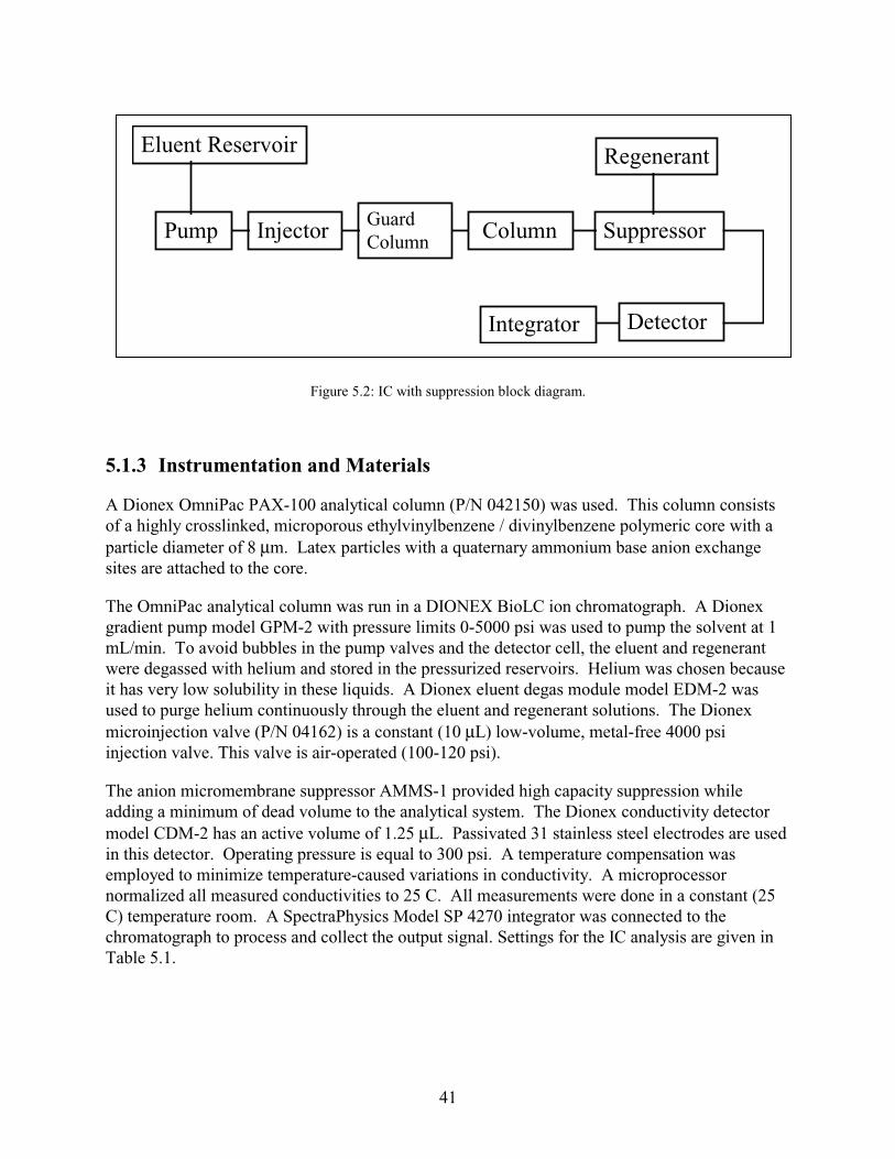
Eluent Reservoir

Pump Injector Guard Column Column Suppressor

Regenerant

DetectorIntegrator

Figure 5.2: IC with suppression block diagram.

5.1.3 Instrumentation and Materials

A Dionex OmniPac PAX-100 analytical column (P/N 042150) was used. This column consists of a highly crosslinked, microporous ethylvinylbenzene / divinylbenzene polymeric core with a particle diameter of 8 µm. Latex particles with a quaternary ammonium base anion exchange sites are attached to the core.

The OmniPac analytical column was run in a DIONEX BioLC ion chromatograph. A Dionex gradient pump model GPM-2 with pressure limits 0-5000 psi was used to pump the solvent at 1 mL/min. To avoid bubbles in the pump valves and the detector cell, the eluent and regenerant were degassed with helium and stored in the pressurized reservoirs. Helium was chosen because it has very low solubility in these liquids. A Dionex eluent degas module model EDM-2 was used to purge helium continuously through the eluent and regenerant solutions. The Dionex microinjection valve (P/N 04162) is a constant (10 µL) low-volume, metal-free 4000 psi injection valve. This valve is air-operated (100-120 psi).

The anion micromembrane suppressor AMMS-1 provided high capacity suppression while adding a minimum of dead volume to the analytical system. The Dionex conductivity detector model CDM-2 has an active volume of 1.25 µL. Passivated 31 stainless steel electrodes are used in this detector. Operating pressure is equal to 300 psi. A temperature compensation was employed to minimize temperature-caused variations in conductivity. A microprocessor normalized all measured conductivities to 25 C. All measurements were done in a constant (25 C) temperature room. A SpectraPhysics Model SP 4270 integrator was connected to the chromatograph to process and collect the output signal. Settings for the IC analysis are given in Table 5.1.

41

Table 5.1: IC instrumental settings.

Name of setting

low limit pressurehigh limit pressureeluent flow ratedegas module pressurepressure at regenerant bottleconductivity rangetemperature coeficientauto offsetattenuationpeak widthpeak threshold

0 psi3000 psi1 mL / min7 psi7-10 psi30 uS1.7on10246200

The eluent solution contained 3.9 mM NaHCO3, 3.1 mM Na2CO3 and 5 % (v/v) EtOH. Mallinckrodt AR sodium bicarbonate (assay 100.2 %, chloride < 3E-3 %), Mallinckrodt AR sodium carbonate anhydrous (chloride < 7E-4 %), and dehydrated Absolute-200 Proof ethanol were used to prepare this solution. DI water generated from a Millipore Milli-Q system was used. To eliminate clogging of the column, the eluent solution was vacuum filtered through an Applied Science Labs Nylon 66 membrane, 0.2 micrometer. Mallinckrodt AR sulfuric acid (assay 96.3 %, chloride < 5E-6 %) was used to prepare 1 mM regenerant solution.

5.1.4 Sample Preparation and Analysis Procedure

Digestion of mortar powder for chloride analysis by IC was done by a water extraction technique. First, a sample of about 0.2 - 0.5 g was weighed on the Mettler AE240 analytical balance (resolution 0.0001 g) and transferred to the 50 mL beaker. About 30 mL of DI water was added to the same beaker. Then, the beaker was covered with a watch glass and rapidly brought to boiling for 5 minutes. After cooling to room temperature, the sample was filtered by vacuum filtration through a Whatman Glass Microfibre Filter GF/A. The sides of the beaker and the sediment remaining in the beaker were washed out with DI water and this portion of the sample was combined with the solution in the filter. Thereafter, the filtered solution was transferred to a 100-mL volumetric flask and diluted to the mark with DI water.

Depending on the goal of the experiments (see Section 5.1.5) and the range of the analyte concentrations to be determined, standard solutions were prepared with concentrations of 1, 5, 10, 15 mgCl/L or with concentrations of 1, 2.5, 5, 7.5 mg/L, in either a mortar extract matrix or a water matrix. The mortar extract matrix was prepared by extracting 0.5 g of mortar powder obtained from a mortar blank block (nominal chloride concentration 0 mg/g) according to the sample preparation procedure discussed earlier in this section. Mallinckrodt AR (assay 99.8 %) sodium chloride was used to prepare the stock solution with chloride content of 100 mg/L.

42

Before chromatographic measurements the column was equilibrated for about 15 minutes until the baseline was stable before. Several calibrations were performed in the course of each analysis at intervals of 2 - 3 hours. Each standard solution was injected one time during calibration.

To obtain maximum precision in the injections, the complete-filling method was used. An injected sample volume was about 5 volumes of the actual loop (10 µL). To prevent clogging of the column, samples and standard solutions were filtered through Corning Nylon Membrane polypropylene sterile filters (0.2 µm) with a 5 mL HSW disposable sterile syringe. Before each injection the filter and syringe were rinsed 3 times with DI water and then 3 times with the solution to be injected. Typical chromatograms for standard and sample solutions are shown in Figure 5.3.

a) b)

Figure 5.3: Typical chromatograms: a) standard solution in water matrix, chloride concentration 5 mg/L, retention time 2.56 min; b) mortar block sample, nominal chloride concentration 4.24 mg/L, retention time 2.53 min.

The work done on chloride analysis by IC can be divided into two major parts. The first part was aimed at the development of a method of calibration and the determination of accuracy and reproducibility of the measurements. In the process of optimization of the method of calibration, the effect of mortar matrix on peak height and peak area was evaluated. To estimate the

43

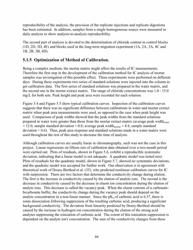
reproducibility of the analysis, the precision of the replicate injections and replicate digestions has been estimated. In addition, samples from a single homogeneous source were measured in daily analysis to show analysis-to-analysis reproducibility.

The second part of analysis is devoted to the determination of chloride content in control blocks (1D, 2D, 3D, 4E) and blocks used in the long-term migration experiment (1A, 2A, 3A, 4C and 1B, 2B, 3B, 4D).

5.1.5 Optimization of Method of Calibration.

Being a complex medium, the mortar matrix might affect the results of IC measurements. Therefore the first step in the development of the calibration method for IC analysis of mortar samples was investigation of this possible effect. Three experiments were performed on different days. During these experiments two series of standard solutions were injected into the column to get calibration data. The first series of standard solutions was prepared in the water matrix, and the second one in the mortar extract matrix. The range of chloride concentrations was 1.0 - 15.0 mg/L for both sets. Peak height and peak area were recorded for each solution.

Figure 5.4 and Figure 5.5 show typical calibration curves. Inspection of the calibration curves suggests that there was no significant difference between calibrations in water and mortar extract matrix when peak area measurements were used, as opposed to the case when peak height was used. Comparison of peak widths showed that the peak widths from the standard solutions prepared in water were greater than those from the mortar extract matrix (average peak widthwater

= 12.0, sample standard deviation = 0.8; average peak widthmortar = 8.8, sample standard deviation = 0.6). Thus, peak area response and standard solutions made in a water matrix were used throughout the rest of this study to decrease the time of analysis.

Although calibration curves are usually linear in chromatography, such was not the case in this project. Linear regressions on fifteen sets of calibration data obtained over a two-month period were carried out. Plots of residuals, shown in Figure 5.6, exhibit a reproducible systematic deviation, indicating that a linear model is not adequate. A quadratic model was tested next. Plots of residuals for the quadratic model, shown in Figure 5.7, showed no systematic deviations, and the quadratic model was accepted for further work. Our observation is in agreement with theoretical work of Doury-Berthod et al. (35), who predicted nonlinear calibration curves for IC with surpression. There are two factors that determine the conductivity change during elution. The first is the increase in conductivity caused by the elution of analyte ions. The second is the decrease in conductivity caused by the decrease in eluent ion concentration during the elution of analyte ions. This decrease is called the vacancy peak. When the eluent consists of a carbonate-bicarbonate buffer, the conductivity change during the vacancy peak should depend on the analyte concentration in a non-linear manner. Since the pKa of carbonic acid is 6.37, there is some dissociation following suppression of the resulting carbonic acid, producing a significant background conductivity. The deviation from linearity predicted by Doury-Berthod should be caused by the increase in hydrogen ion concentration during the elution of the strong acid analytes suppressing the ionization of carbonic acid. The extent of this ionization suppression is dependent on the analyte ion's concentration. The sum of the conductivity changes from these

44

factors should produce a nonlinear calibration curve. Table 5.2 provides standard errors for each coefficient of all calibration curves.

0.0E+00

1.0E+05

2.0E+05

3.0E+05

4.0E+05

5.0E+05

0 5 10 15 20

Chloride concentration, mg / L

Peak

hei

ght

Mortar matrix

Water matrix

Figure 5.4: Comparison of typical calibration curves in water and mortar extract matrices obtained with peak height measurements. Standards with water matrix: slope = 23722, intercept = 4459. Standards with mortar extract

matrix: slope = 31141, intercept = 4619.

45

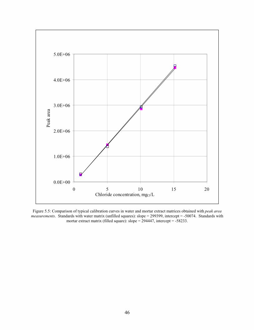
0.0E+00

1.0E+06

2.0E+06

3.0E+06

4.0E+06

5.0E+06

0 5 10 15 20 Chloride concentration, mgCl/L

Peak

are

a

Figure 5.5: Comparison of typical calibration curves in water and mortar extract matrices obtained with peak area measurements. Standards with water matrix (unfilled squares): slope = 299399, intercept = -50074. Standards with

mortar extract matrix (filled square): slope = 294447, intercept = -58233.

46

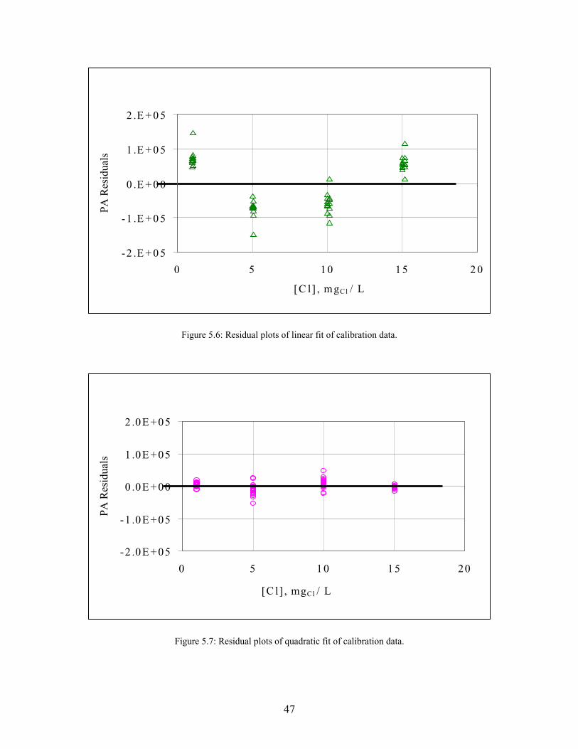
-2 .E + 0 5

-1 .E + 0 5

0 .E + 0 0

1 .E + 0 5

2 .E + 0 5

0 5 1 0 1 5 2 0

[C l ] , m gC l / L

PA R

esid

uals

Figure 5.6: Residual plots of linear fit of calibration data.

-2 .0 E + 0 5

-1 .0 E + 0 5

0 .0E +0 0

1 .0E +0 5

2 .0E +0 5

0 5 10 15 2 0

[C l] , m gCl / L

PA R

esid

uals

Figure 5.7: Residual plots of quadratic fit of calibration data.

47

Table 5.2: Regression coefficients and their standard errors

Date Quadratic Std error in Linear Std error in Intercept Std error in term quadratic term term linear term intercept

8/16/96 3402 396 237304 6643 83806 21434 2598 775 257162 12992 47806 41922

8/20/96 3104 1080 249729 18102 36753 58409 3192 224 245208 3760 48893 12132

8/27/96 2957 879 285747 48274 61442 155765 2739 402 249300 6732 41497 21723

9/2/96 2016 1837 261924 32596 -28449 110516 9/8/96 2872 494 287368 8758 -26711 29694

2984 786 245921 13957 95336 47322 10/5/96 2547 725 254147 12016 32070 38342

2805 510 237754 8450 43511 26961 10/16/96 2296 149 252443 2468 40926 7875

2572 614 249096 10188 26122 32508 10/30/96 3658 4 238497 58 -3463 186

3122 391 226456 6486 -7683 20696

5.1.6 Reproducibility of Analysis

To evaluate reproducibility of the method we calculated the standard deviation in repeated measurements. Table 5.3 shows the relative standard deviations of peak area signals for replicate injections of standard and sample solutions. These values were better than 1%. Next we considered reproducibility of multiple digestions.

To estimate the precision of the analysis among multiple digestions (replicates), all available data obtained during the IC measurements of the thirteen mortar blocks were divided in two groups. The first group includes data for control blocks and test blocks samples, Table 5.4. The second group, Table 5.5, contains data obtained for Block 7, the new block cast with nominal chloride content of 1.45 mg/g, which was never subjected to polarization. As mentioned in Section 3.1, this block was cured separately from the other blocks and was not subjected to polarization. After curing, the block was drilled to obtain a large portion of mortar powder, which was then homogenized and used to prepare reference sample solutions for each IC analysis. Thus, samples from Block 7 should be free from sampling variability.

Analysis of these two sets of data shows that the range of deviations from the average chloride concentrations of multiple digestions of control blocks and blocks used in the migration experiment was 0 - 3 % (excluding two outliers, 10.4 % and 7.3), Table 5.4. The range of deviations obtained from the analyses of Block 7 multiple digestions was 2.0 - 3.1 %, Table 5.5. Thus, it was concluded that the scatter in the chloride concentration for multiple digestions of mortar samples was typically better than 3.1 %.

48

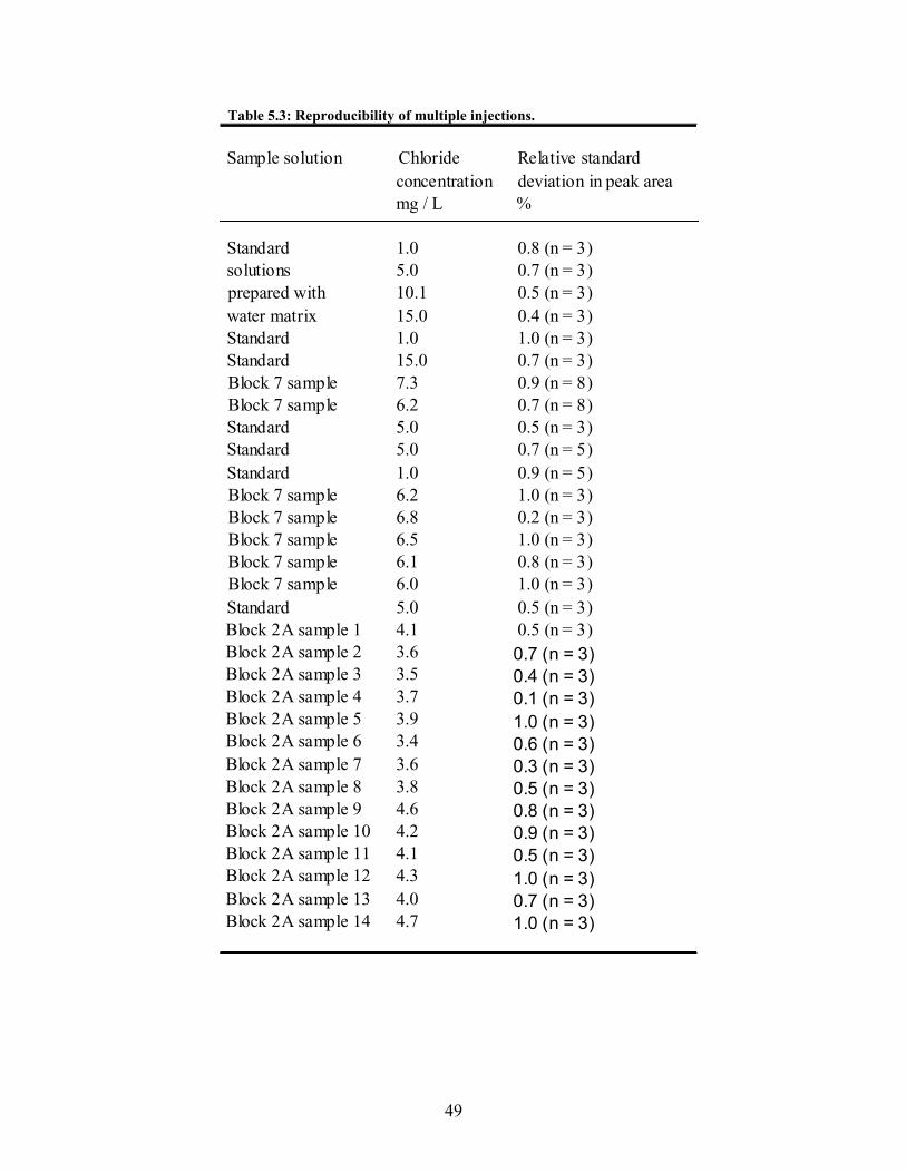
Table 5.3: Reproducibility of multiple injections.

Sample solution Chloride Relative standard concentration deviation in peak area mg / L %

Standard 1.0 0.8 (n = 3) solutions 5.0 0.7 (n = 3) prepared with 10.1 0.5 (n = 3) water matrix 15.0 0.4 (n = 3) Standard 1.0 1.0 (n = 3) Standard 15.0 0.7 (n = 3) Block 7 sample 7.3 0.9 (n = 8) Block 7 sample 6.2 0.7 (n = 8) Standard 5.0 0.5 (n = 3) Standard 5.0 0.7 (n = 5) Standard 1.0 0.9 (n = 5) Block 7 sample 6.2 1.0 (n = 3) Block 7 sample 6.8 0.2 (n = 3) Block 7 sample 6.5 1.0 (n = 3) Block 7 sample 6.1 0.8 (n = 3) Block 7 sample 6.0 1.0 (n = 3) Standard 5.0 0.5 (n = 3) Block 2A sample 1 4.1 0.5 (n = 3) Block 2A sample 2 3.6 0.7 (n = 3) Block 2A sample 3 3.5 0.4 (n = 3) Block 2A sample 4 3.7 0.1 (n = 3) Block 2A sample 5 3.9 1.0 (n = 3) Block 2A sample 6 3.4 0.6 (n = 3) Block 2A sample 7 3.6 0.3 (n = 3) Block 2A sample 8 3.8 0.5 (n = 3) Block 2A sample 9 4.6 0.8 (n = 3) Block 2A sample 10 4.2 0.9 (n = 3) Block 2A sample 11 4.1 0.5 (n = 3) Block 2A sample 12 4.3 1.0 (n = 3) Block 2A sample 13 4.0 0.7 (n = 3) Block 2A sample 14 4.7 1.0 (n = 3)

49

Table 5.3: (continued)

Sample solution Concentration Relative standard deviation in peak area

mg / L %

Block 2B sample 1 3.1 0.2 (n = 3) Block 2B sample 2 3.8 0.6 (n = 3) Block 2B sample 3 3.9 0.2 (n = 3) Block 2B sample 4 3.4 0.2 (n = 3) Block 2B sample 5 3.6 0.2 (n =3) Block 2B sample 6 3.2 0.5 (n = 3) Block 2B sample 7 3.6 0.2 (n = 3) Block 2B sample 8 3.7 0.5 (n = 3) Block 2B sample 9 2.5 0.5 (n = 3) Block 2B sample 10 4.4 0.4 (n = 3) Block 2B sample 11 4.0 0.2 (n = 3) Standard 1.0 0.3 (n = 5) Standard 2.5 0.2 (n = 5) Standard 5.0 0.1 (n = 5) Standard 7.5 0.2 (n = 5) Standard 10.0 0.1 (n = 5) Standard 5.0 0.6 (n = 3) Block 1B sample 1.7 0.0 (n = 3) Standard 5.0 0.1 (n = 3) Standard 7.5 0.4 (n = 3) Standard 5.0 0.4 (n =3) Standard 7.5 0.7 (n = 3) Block 3B sample 3.3 0.8 (n = 3) Standard 5.0 0.3 (n = 3) Block 7 sample 4.1 0.2 (n =3) Standard 5.0 0.4 (n = 5) Block 4C sample 4.3 1.0 (n = 3)

50

Table 5.4: Reproducibility of multiple digestions of mortar block samples.

Block ID Number of Average Deviation (n=2) or % Deviation multiple chloride standard deviation (dev. / avg.*100) digestions from average (n=3)

mg / g mg / g

Control 1D 2 2 2 2 2 2 2 3 2 2 2 2

Control 2D 2 2 2 2 2 2 3 3 2 3 3 3 3

Control 3D 2 2 2 2 2

0.36 0.32 0.26 0.24 0.27 0.33 0.25 0.23 0.18 0.21 0.31 0.37 0.80 0.90 0.84 0.77 0.66 0.80 0.64 0.67 0.68 0.72 0.61 0.54 0.58 0.69 0.68 0.57 0.61 0.51

7.56E-03 3.89E-03 9.83E-04 3.03E-03 7.29E-03 4.19E-03 1.32E-03 1.60E-03 7.09E-04 5.04E-03 5.98E-03 6.48E-04 9.11E-05 5.88E-03 3.59E-03 3.01E-03 5.11E-04 1.11E-03 1.28E-02 9.34E-03 1.30E-03 1.30E-02 1.32E-02 8.92E-03 1.52E-02 1.86E-02 6.43E-03 5.41E-03 1.77E-02 1.54E-02

2.1 1.2 0.4 1.3 2.7 1.3 0.5 0.7 0.4 2.4 1.9 0.2 0.0 0.7 0.4 0.4 0.1 0.1 2.0 1.4 0.2 1.8 2.2 1.7 2.6 2.7 0.9 1.0 2.9 3.0

.

51

Table 5.4: (continued)

Block ID Number of Average Deviation (n=2) or % Deviation multiple chloride standard deviation (dev. / avg.*100) digestions from average (n=3)

mg / g mg / g

Control 4E 2 1.13 1.06E-02 0.9 2 0.81 1.22E-02 1.5 2 1.03 9.20E-04 0.1 2 1.13 1.05E-02 0.9 2 0.94 9.81E-02 1 0 .4 2 1.04 6.60E-03 0.6 2 1.45 1.06E-01 7 .3 2 1.96 1.93E-02 1.0 2 2.00 3.00E-04 0.0

Block 1A 2 0.31 1.00E-03 0.3 2 0.28 3.70E-03 1.3 2 0.29 4.00E-03 1.4

Block 3A 2 0.60 1.52E-02 2.5 2 0.52 8.50E-03 1.6 2 0.59 1.40E-03 0.2

Block 4C 3 1.58 1.84E-02 1.2 3 1.63 1.96E-02 1.2 2 1.75 1.13E-02 0.6 2 1.71 4.00E-04 0.0 3 1.35 1.35E-02 1.0 3 1.93 5.10E-02 2.6 3 1.86 3.06E-02 1.6 3 1.55 2.79E-02 1.8 2 1.73 2.84E-04 0.0

Block 1B 2 0.29 6 .0 9 E -0 3 2 .1 2 0.30 6.44E-03 2.1 2 0.31 7.95E-03 2.6 2 0.31 7.00E-03 2.3 2 0.33 5.51E-03 1.7 2 0.32 1.62E-03 0.5 2 0.36 2.00E-03 0.5 2 0.39 1.06E-02 2.7

Block 2B 2 0.62 5.34E-03 0.9 2 0.67 7.19E-03 1.1 2 0.70 7.85E-03 1.1

52

Table 5.4: (continued)

Block ID Number of Average Deviation (n=2) or % Deviation multiple chloride standard deviation (dev. / avg.*100) digestions from average (n=3)

mg / g mg / g

Block 3B Block 4D

2 0.59 4.70E-03 0.8 2 1.53 1.87E-02 1.2 2 1.49 1.11E-02 0.7 2 1.46 3.65E-02 2.5 2 1.50 1.33E-02 0.9 2 1.54 3.36E-02 2.2 3 1.58 8.35E-03 0.5 3 1.59 1.59E-02 1.0 2 1.43 2.01E-02 1.4 2 1.72 9.08E-03 0.5 3 1.73 1.88E-02 1.1 2 1.80 2.43E-02 1.4 3 1.63 3.03E-02 1.9 2 1.85 1.21E-02 0.7 2 1.99 3.60E-03 0.2

Table 5.5: Reproducibility of multiple digestions of block 7 samples.

Block ID Number of Average Standard deviation Relative standard multiple chloride from average deviation digestions mg / g mg / g %

Block 7 8 1.2783 0.0401 3.1 8 1.2425 0.0245 2.0 3 1.3023 0.0312 2.4 8 1.2359 0.0381 3.1 3 1.2304 0.0258 2.1

To monitor the stability of the IC chloride analysis a control chart was maintained over whole time period of measurements. Samples from mortar Block 7 were used for this purpose. Approximately 0.5 g of mortar powder was taken each time to yield a chloride concentration of about 6 - 7 mg/L. The water extraction procedure, Section 5.1.4, was used. The daily average

53

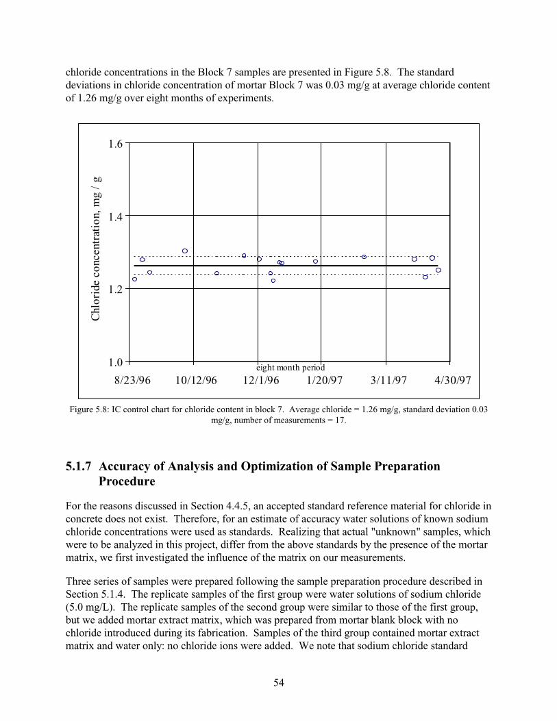
chloride concentrations in the Block 7 samples are presented in Figure 5.8. The standard deviations in chloride concentration of mortar Block 7 was 0.03 mg/g at average chloride content of 1.26 mg/g over eight months of experiments.

1.0

1.2

1.4

1.6

8/23/96 10/12/96 12/1/96 1/20/97 3/11/97 4/30/97

Chl

orid

e co

ncen

trat

ion,

mg

/ g

eight month period

Figure 5.8: IC control chart for chloride content in block 7. Average chloride = 1.26 mg/g, standard deviation 0.03 mg/g, number of measurements = 17.

5.1.7 Accuracy of Analysis and Optimization of Sample Preparation Procedure

For the reasons discussed in Section 4.4.5, an accepted standard reference material for chloride in concrete does not exist. Therefore, for an estimate of accuracy water solutions of known sodium chloride concentrations were used as standards. Realizing that actual "unknown" samples, which were to be analyzed in this project, differ from the above standards by the presence of the mortar matrix, we first investigated the influence of the matrix on our measurements.

Three series of samples were prepared following the sample preparation procedure described in Section 5.1.4. The replicate samples of the first group were water solutions of sodium chloride (5.0 mg/L). The replicate samples of the second group were similar to those of the first group, but we added mortar extract matrix, which was prepared from mortar blank block with no chloride introduced during its fabrication. Samples of the third group contained mortar extract matrix and water only: no chloride ions were added. We note that sodium chloride standard

54

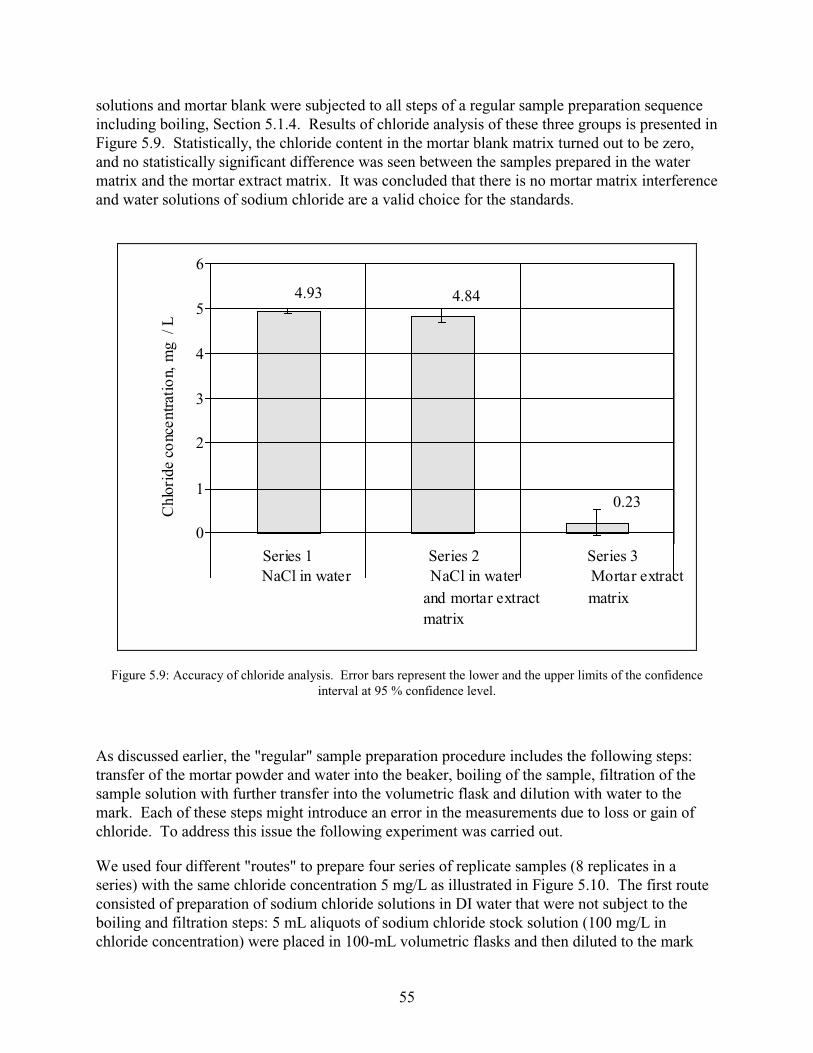
solutions and mortar blank were subjected to all steps of a regular sample preparation sequence including boiling, Section 5.1.4. Results of chloride analysis of these three groups is presented in Figure 5.9. Statistically, the chloride content in the mortar blank matrix turned out to be zero, and no statistically significant difference was seen between the samples prepared in the water matrix and the mortar extract matrix. It was concluded that there is no mortar matrix interference and water solutions of sodium chloride are a valid choice for the standards.

4.93

0.23

4.84

0

1

2

3

4

5

6

Chl

orid

e co

ncen

tratio

n, m

g / L

Series 1 ies 2 eries 3 NaCl in water NaCl in water Mortar extract

and mortar extract matrix matrix

Ser S

Figure 5.9: Accuracy of chloride analysis. Error bars represent the lower and the upper limits of the confidence interval at 95 % confidence level.

As discussed earlier, the "regular" sample preparation procedure includes the following steps: transfer of the mortar powder and water into the beaker, boiling of the sample, filtration of the sample solution with further transfer into the volumetric flask and dilution with water to the mark. Each of these steps might introduce an error in the measurements due to loss or gain of chloride. To address this issue the following experiment was carried out.

We used four different "routes" to prepare four series of replicate samples (8 replicates in a series) with the same chloride concentration 5 mg/L as illustrated in Figure 5.10. The first route consisted of preparation of sodium chloride solutions in DI water that were not subject to the boiling and filtration steps: 5 mL aliquots of sodium chloride stock solution (100 mg/L in chloride concentration) were placed in 100-mL volumetric flasks and then diluted to the mark

55

with DI water. The second route was similar to the first with the exception that about 0.5 g of mortar powder from the mortar blank block were transferred into the flask before dilution. In the third route, samples were similar to those from the second route, but they were subjected to the boiling step before dilution. The forth route differed from the third one by addition of a filtration operation between the boiling and dilution steps. The experimental results for all four series of samples, shown in Figure 5.11, suggest that there was neither loss nor gain of chloride during a regular sample preparation procedure: statistically all four measurements are indistinguishable since their confidence intervals overlap.

Mortar Blank

Drilling

Boiling

Filtration

Dilution

NaCl

NaCl

2

4

3

4

DI Water

1

3 & 4

Figure 5.10: Schematic representation of four sample preparation routes.

56

4.96 5.01 4.96 5.05

0

1

2

3

4

5

6

Chl

orid

e co

ncen

trat

ion,

mg C

l / L

Series 1 No boiling No filtration No mortar

Series 2 No boiling No filtration Mortar matrix

Series 3 Boiling No filtration Mortar matrix

Series 4 Boiling Filtration Mortar matrix

Figure 5.11: Results of investigation of possible loss or gain of chloride during sample preparation. Error bars represent the lower and the upper limits of the confidence interval at 95 % confidence level.

One of the most time consuming steps in the regular sample preparation procedure is the filtration step. In the previous experiment we had indications that the filtration step does not affect concentration measurements. Another test was performed to check this hypothesis. This time we analyzed a "real" sample, prepared from the chloride containing block, as opposed to the sample simulation in the chloride gain/loss experiment. Sixteen samples were made from mortar Block 7 (nominal chloride 1.45 mg/g). For the first eight samples the filtration step after boiling / cooling operation was skipped. The rest of the samples were subject to the regular preparation. In the course of analysis it was determined that the average chloride concentration of samples prepared without filtration was 1.29 mg/g (sample standard deviation = 0.02 mg/g) and the average chloride concentration of samples prepared by the regular procedure was 1.24 mg/g (sample standard deviation = 0.04 mg/g), as shown in Figure 5.12. The confidence intervals of both measurements overlap and there is no statistical difference between them. Thus, it was confirmed that filtration of mortar samples does not give any improvement and can be omitted from the sample preparation procedure.

57

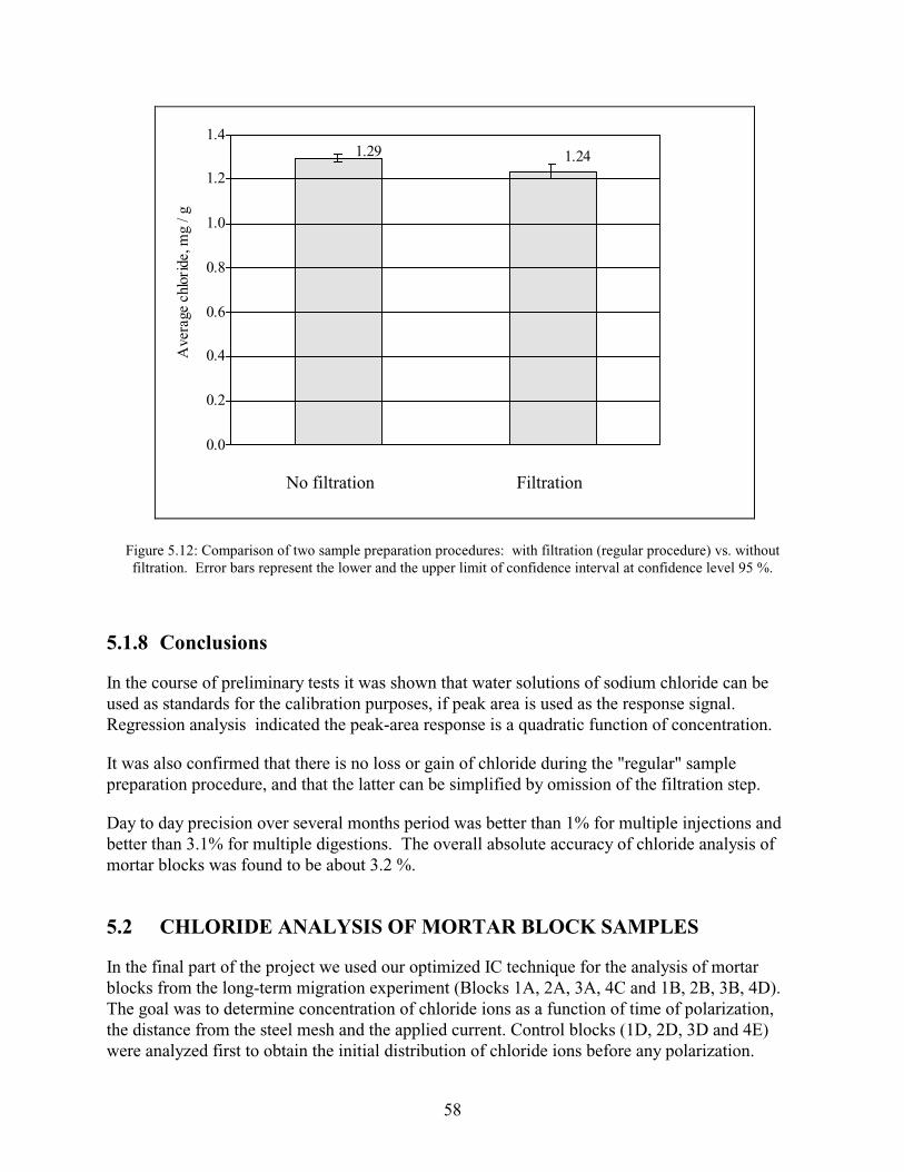
1.241.29

0.0

0.2

0.4

0.6

0.8

1.0

1.2

1.4

Ave

rage

chl

orid

e, m

g / g

No filtration iltration F

Figure 5.12: Comparison of two sample preparation procedures: with filtration (regular procedure) vs. without filtration. Error bars represent the lower and the upper limit of confidence interval at confidence level 95 %.

5.1.8 Conclusions

In the course of preliminary tests it was shown that water solutions of sodium chloride can be used as standards for the calibration purposes, if peak area is used as the response signal. Regression analysis indicated the peak-area response is a quadratic function of concentration.

It was also confirmed that there is no loss or gain of chloride during the "regular" sample preparation procedure, and that the latter can be simplified by omission of the filtration step.

Day to day precision over several months period was better than 1% for multiple injections and better than 3.1% for multiple digestions. The overall absolute accuracy of chloride analysis of mortar blocks was found to be about 3.2 %.

5.2 CHLORIDE ANALYSIS OF MORTAR BLOCK SAMPLES

In the final part of the project we used our optimized IC technique for the analysis of mortar blocks from the long-term migration experiment (Blocks 1A, 2A, 3A, 4C and 1B, 2B, 3B, 4D). The goal was to determine concentration of chloride ions as a function of time of polarization, the distance from the steel mesh and the applied current. Control blocks (1D, 2D, 3D and 4E) were analyzed first to obtain the initial distribution of chloride ions before any polarization.

58

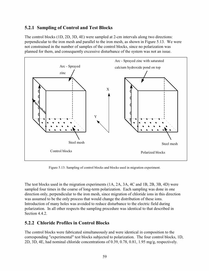
5.2.1 Sampling of Control and Test Blocks

The control blocks (1D, 2D, 3D, 4E) were sampled at 2-cm intervals along two directions: perpendicular to the iron mesh and parallel to the iron mesh, as shown in Figure 5.13. We were not constrained in the number of samples of the control blocks, since no polarization was planned for them, and consequently excessive disturbance of the system was not an issue.

Steel mesh

Arc - Sprayed zinc with saturated

calcium hydroxide pond on top

Steel mesh

Arc - Sprayed

zinc

Control blocks Polarized blocks

X

Y

Figure 5.13: Sampling of control blocks and blocks used in migration experiment.

The test blocks used in the migration experiments (1A, 2A, 3A, 4C and 1B, 2B, 3B, 4D) were sampled four times in the coarse of long-term polarization. Each sampling was done in one direction only, perpendicular to the iron mesh, since migration of chloride ions in this direction was assumed to be the only process that would change the distribution of these ions. Introduction of many holes was avoided to reduce disturbance to the electric field during polarization. In all other respects the sampling procedure was identical to that described in Section 4.4.2.

5.2.2 Chloride Profiles in Control Blocks

The control blocks were fabricated simultaneously and were identical in composition to the corresponding "experimental" test blocks subjected to polarization. The four control blocks, 1D, 2D, 3D, 4E, had nominal chloride concentrations of 0.39, 0.78, 0.81, 1.95 mg/g, respectively.

59

Typical chloride profiles in control blocks both "parallel" and "perpendicular" to the iron mesh are shown in Figure 5.14, Figure 5.15, Figure 5.16, and Figure 5.17. A summary for all control blocks is given in Figure 5.18 and Table 5.7.

Two main observations can be made based on the control blocks profiles. First, in all control blocks, the average chloride concentration in both directions of sampling is below the nominal concentration, except for the profile along the line perpendicular to steel mesh in block 2D (Average = 0.78 mg/g, standard deviation = 0.08 mg/g, number of sampling points =6). This fact might be explained by either bleeding of mortar during curing or by incomplete extraction of chloride from mortar by water or both.

Second, there is a relatively large random scatter in the average chloride concentration for all control blocks. The range of relative standard deviations is from 9.6 to 33.4 %, which by far is larger than the uncertainty of the IC analysis (~ 3.1 %). This result is a direct indication of the heterogeneity of the chloride ion distribution in the control blocks. The control chart based on samples from Block 7 (Figure 5.8 in Section 5.1.6), did not point to any experimental problems on the days on which the control-block samples were analyzed.

Table 5.6: Regression coefficients of quadratic fit of calibration data used for analyses of control blocks.

Subject of analysis Quadratic term Linear term Intercept

Control block 4E

Control block 3D

Control block 2D

Control block 1D

2912 236761 -8820 3124 248844 -4849 2296 247190 62550 3322 231681 -3336 3972 226191 17736 3626 231891 35508 2503 236719 -13282 3445 233114 1335 1944 257216 -14202 2265 243544 -5950 2608 228709 31155 3085 252276 10420

60

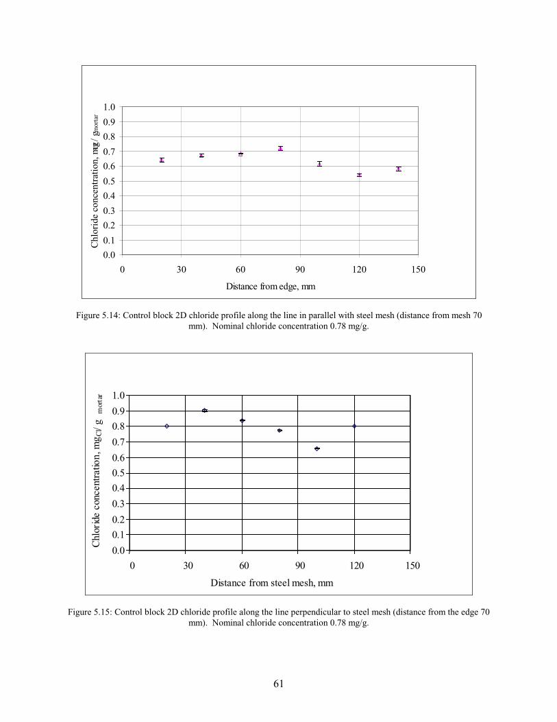
Figure 5.14: Control block 2D chloride profile along the line in parallel with steel mesh (distance from mesh 70 mm). Nominal chloride concentration 0.78 mg/g.

0.0

0.1

0.2

0.3

0.4

0.5

0.6

0.7

0.8

0.9

1.0

0 30 60 90 120 150

Distance from steel mesh, mm

Chl

orid

e co

ncen

trat

ion,

mg C

l/ g

mor

t ar

Figure 5.15: Control block 2D chloride profile along the line perpendicular to steel mesh (distance from the edge 70mm). Nominal chloride concentration 0.78 mg/g.

0.0

0.1

0.2

0.3

0.4

0.5

0.6

0.7

0.8

0.9

1.0

0 30 60 90 120 150

Distance from edge, mm

Chl

orid

e co

ncen

trat

ion,

mg Cl /

g mor

tar

61

0.0

0.2

0.4

0.6

0.8

1.0

1.2

1.4

1.6

1.8

2.0

2.2

0 30 60 90 120 150

Distance from Edge, mm

Chl

orid

e co

ncen

trat

ion,

mg/

g

Figure 5.16: Control block 4E chloride profile along the line in parallel with steel mesh (distance from mesh 70 mm). Nominal chloride concentration 1.95 mg/g.

0.0

0.4

0.8

1.2

1.6

2.0

Ave

rage

chl

orid

e co

ncen

trat

ion,

m

g C

l / g

mor

t ar

Block 1D lock 2D lock 3D lock 4E B B B

Figure 5.17: Average chloride concentration in control blocks in two directions with respect to steel mesh: left columns - parallel, middle columns - perpendicular direction. Right columns show the nominal chloride

concentration. Error bars represent standard deviations from the average chloride content.

62

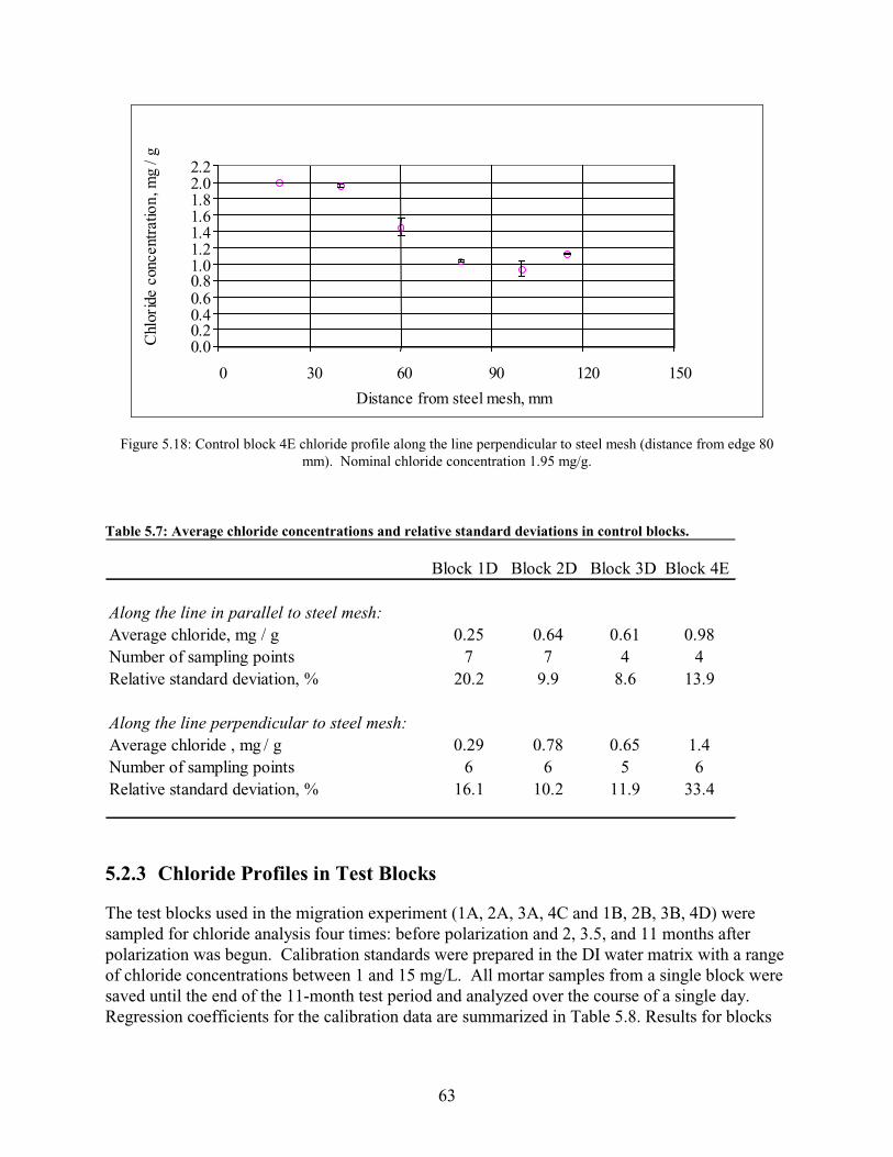
0.0 0.2 0.4 0.6 0.8 1.0 1.2 1.4 1.6 1.8 2.0 2.2

0 0 60 90 120 150

Distance from steel mesh, mm

Chl

or id

e co

ncen

trat

ion,

mg

/ g

3

Figure 5.18: Control block 4E chloride profile along the line perpendicular to steel mesh (distance from edge 80 mm). Nominal chloride concentration 1.95 mg/g.

Table 5.7: Average chloride concentrations and relative standard deviations in control blocks.

Block 1D Block 2D Block 3D Block 4E

Along the line in parallel to steel mesh: Average chloride, mg / g 0.25 0.64 0.61 0.98 Number of sampling points 7 7 4 4 Relative standard deviation, % 20.2 9.9 8.6 13.9

Along the line perpendicular to steel mesh: Average chloride , mg / g 0.29 0.78 0.65 1.4 Number of sampling points 6 6 5 6 Relative standard deviation, % 16.1 10.2 11.9 33.4

5.2.3 Chloride Profiles in Test Blocks

The test blocks used in the migration experiment (1A, 2A, 3A, 4C and 1B, 2B, 3B, 4D) were sampled for chloride analysis four times: before polarization and 2, 3.5, and 11 months after polarization was begun. Calibration standards were prepared in the DI water matrix with a range of chloride concentrations between 1 and 15 mg/L. All mortar samples from a single block were saved until the end of the 11-month test period and analyzed over the course of a single day. Regression coefficients for the calibration data are summarized in Table 5.8. Results for blocks

63

1A, 1B, 2A, 2B, 3A, 3B, 4C and 4D are given in Figure 5.19, Figure 5.20, Figure 5.21, Figure 5.22, Figure 5.23, 24, Figure 5.25 and Figure 5.26, respectively.

Table 5.8: Regression coefficients of quadratic fit of calibration data used for analyses of test blocks.

Subject of analysis Quadratic term Linear term Intercept

Block 1A

Block 2A

Block 2B

Block 1B

Block 3A

Block 3B

Block 4D

Block 4C

2915 239381 11654 1444 273493 -19238 2738 247518 26703 2730 227432 15328 3623 217262 25340 5194 217178 21360 2156 241078 3919 2444 246562 1630 2704 242814 9739 4665 224126 815 3937 228402 -466 3735 230152 -1824 3447 236330 13890 3257 240329 9584 3108 241870 6984 4048 231762 14123 2881 243494 7993 3083 242203 8497 2084 249746 4229 2084 250079 4229 2129 247705 13192 3646 233317 15442 2605 239468 16529 1168 254962 3026 1271 252824 9157 1140 254032 16218 2694 240231 20952 2666 235747 26849 3212 229430 33096

64

0.0

0.1

0.2

0.3

0.4

0.5

0 30 60 90 120 150 Distance from mesh, mm

Chl

orid

e co

ncen

trat

ion,

mg

/ g

Before polarization, Y=60 mm 2 of months of polarization, Y=100 mm 3.5 months of polarization, Y=70 mm 11months of polarization, Y=90 mm

Figure 5.19: Chloride profile in block 1A (applied current density 0.066 A/m2, nominal chloride concentration 0.39 mg/g, w/c 0.5). Y – distance of profile line from the edge of the block.

65

0.0

0.1

0.2

0.3

0.4

0.5

0 30 60 90 120 150 Distance from mesh, mm

Chl

orid

e co

ncen

trat

ion,

mg

/ g

Before polarization, Y=120 mm 2 months of polarization, Y=100 mm 3.5 months of polarization, Y=70 mm 11 months of polarization, Y=88 mm

Figure 5.20: Chloride profile in block 1B (applied current density 0.033 A/m2, nominal chloride concentration 0.39 mg/g, w/c 0.5). Y – distance of profile line from the edge of the block. Error bars represent standard deviations for

multiple digestions.

66

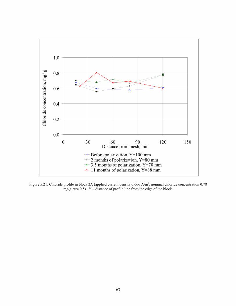
0.0

0.2

0.4

0.6

0.8

1.0

0 30 60 90 120 150 Distance from mesh, mm

Chl

orid

e co

ncen

trat

ion,

mg

/ g

Before polarization, Y=100 mm 2 months of polarization, Y=80 mm 3.5 months of polarization, Y=70 mm 11 months of polarization, Y=88 mm

Figure 5.21: Chloride profile in block 2A (applied current density 0.066 A/m2, nominal chloride concentration 0.78 mg/g, w/c 0.5). Y – distance of profile line from the edge of the block.

67

0.0

0.2

0.4

0.6

0.8

1.0

0 30 60 90 120 150 Distance from mesh, mm

Chl

orid

e co

ncen

trat

ion,

mg

/ g

Before polarization, Y=100 mm 2 months of polarization, Y=80 mm 3.5 months of polarization, Y=70 mm 11 months of polarization, Y=55 mm

Figure 5.22: Chloride profile in block 2B (applied current density 0.033 A/m2, nominal chloride concentration 0.78 mg/g, w/c 0.5). Y – distance of profile line from the edge of the block. Error bars represent standard deviations for

multiple injections.

68

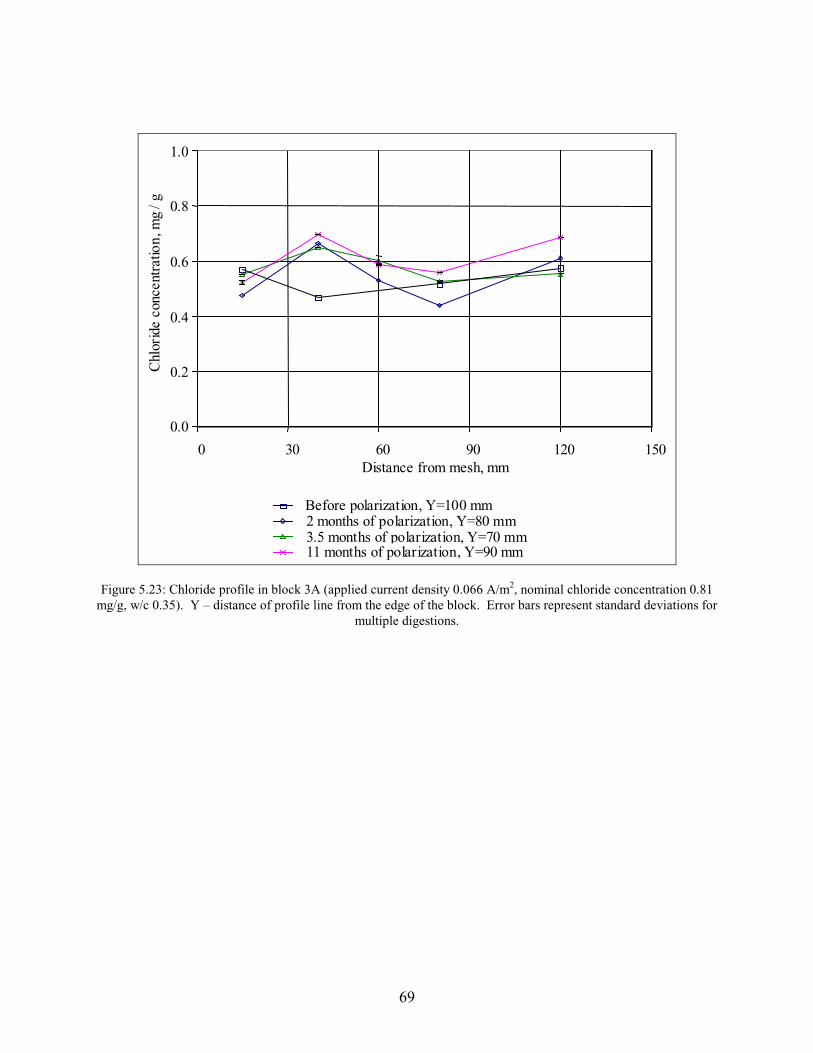
0.0

0.2

0.4

0.6

0.8

1.0

0 30 60 90 120 150 Distance from mesh, mm

Chl

orid

e co

ncen

trat

ion,

mg

/ g

Before polarization, Y=100 mm 2 months of polarization, Y=80 mm 3.5 months of polarization, Y=70 mm 11 months of polarization, Y=90 mm

Figure 5.23: Chloride profile in block 3A (applied current density 0.066 A/m2, nominal chloride concentration 0.81 mg/g, w/c 0.35). Y – distance of profile line from the edge of the block. Error bars represent standard deviations for

multiple digestions.

69

0.0

0.2

0.4

0.6

0.8

1.0

0 30 60 90 120 150 Distance from mesh, mm

Chl

orid

e co

ncen

trat

ion,

mg

/ g

Before polarization, Y=100 mm 2 months of polarization, Y=80 mm 3.5 months of polarization, Y=70 mm 11 months of polarization, Y=89 mm

Figure 5.24: Chloride profile in block 3B (applied current density 0.033 A/m2, nominal chloride concentration 0.81 mg/g, w/c 0.35). Y – distance of profile line from the edge of the block Error bars represent: for point Y = 100 mm,

X = 40 (before polarization) standard deviations for multiple injections; for point Y = 89 mm, X = 40 mm (11 months of polarization) standard deviations for multiple digestions.

70

0.0

0.4

0.8

1.2

1.6

2.0

0 30 0 0 120 150 Distance from mesh, mm

Chl

orid

e co

ncen

trat

ion,

mg

/ g

Before polarization, Y=100 mm 2 months of polarization, Y=80 mm 3.5 months of polarization, Y=70 mm 11 months of polarization, Y=55 mm

6 9

Figure 5.25: Chloride profile in block 4C (applied current density 0.066 A/m2, nominal chloride concentration 1.95 mg/g, w/c 0.5). Y – distance of profile line from the edge of the block. Error bars represent standard deviations for

multiple digestions .

71

0.0

0.4

0.8

1.2

1.6

2.0

0 0 60 90 120 150 Distance from mesh, mm

Chl

orid

e co

ncen

trat

ion,

mg

/ g

Before polarization, Y=100 mm 2 months of polarization, Y=80 mm 3.5 months of polarization, Y=70 mm 11 months of polarization, Y=88 mm

3

Figure 5.26: Chloride profile in block 4D (applied current density 0.033 A/m2, nominal chloride concentration 1.95 mg/g, w/c 0.5). Y – distance of profile line from the edge of the block. Error bars represent standard deviations for

multiple digestions, except one point at Y = 100 mm, X = 80 mm (before polarization) for which standard deviation for multiple injections is shown.

72

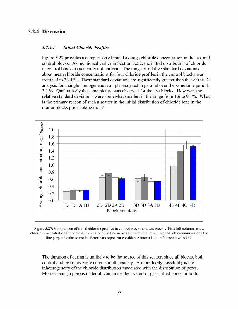
5.2.4 Discussion

5.2.4.1 Initial Chloride Profiles

Figure 5.27 provides a comparison of initial average chloride concentration in the test and control blocks. As mentioned earlier in Section 5.2.2, the initial distribution of chloride in control blocks is generally not uniform. The range of relative standard deviations about mean chloride concentrations for four chloride profiles in the control blocks was from 9.9 to 33.4 %. These standard deviations are significantly greater than that of the IC analysis for a single homogeneous sample analyzed in parallel over the same time period, 3.1 %. Qualitatively the same picture was observed for the test blocks. However, the relative standard deviations were somewhat smaller: in the range from 1.6 to 9.4%. What is the primary reason of such a scatter in the initial distribution of chloride ions in the mortar blocks prior polarization?

0.0

0.2

0.4

0.6

0.8

1.0

1.2

1.4

1.6

1.8

2.0

Ave

rage

chl

orid

e co

ncen

trat

ion,

mg C

l / g

mor

tar

1D 1D 1A 1B 2D 2D 2A 2B 3D 3D 3A 3B 4E 4E 4C Block notations

4D

Figure 5.27: Comparison of initial chloride profiles in control blocks and test blocks. First left columns show chloride concentration for control blocks along the line in parallel with steel mesh, second left columns - along the

line perpendicular to mesh. Error bars represent confidence interval at confidence level 95 %.

The duration of curing is unlikely to be the source of this scatter, since all blocks, both control and test ones, were cured simultaneously. A more likely possibility is the inhomogeneity of the chloride distribution associated with the distribution of pores. Mortar, being a porous material, contains either water- or gas - filled pores, or both.

73

After the mortar has hardened, the water-filled pores may dry, and air-filled pores may become water saturated, depending on the history of mortar, the external moisture conditions, and the dimensions of the mortar sample, (36). Soluble chloride may accumulate in water filled pores, from which the water eventually evaporates. Thus, if pore walls contain a disproportionate amount of chloride, and the pore sizes are not much smaller than the sample size, the samples themselves might be very heterogeneous in chloride concentration. Quantitative investigation of the pore structure is a difficult task and beyond the scope of this work. However, to obtain a qualitative picture, all sides of test blocks used in the migration experiment were examined for cracks and voids. Results of such a visual examination are summarized in Table 5.9. As was expected, pore non-uniformity of the test blocks was confirmed. Visual examination of the control blocks was also carried out but in a different fashion. A cylindrical core from the center of control block 4E was cut through the entire volume. Two sides of the cylinder are pictured in Figure 5.28. As seen from this figure, the distribution of pores inside the block is also highly non-uniform.

As mentioned before, the initial average chloride concentration found in the mortar blocks was generally below the nominal chloride concentrations, as shown in Figure 5.18. This result brings up the issue of bleeding of the mortar blocks during the curing period, as discussed in Section 2.2. Migration of bleed water to the top of blocks could be responsible for a decrease in chloride concentration as well as a non-uniformity in concentration profiles.

Although no quantitative measurements of bleed water were performed, visual observations of the curing blocks showed that bleeding was either extremely small (blocks with water to cement ratio 0.5), or not observed at all (blocks with water to cement ratio 0.35). Therefore, the effect of bleeding on chloride concentration and its distribution was assumed to be minimal if at all.

As mentioned in Section 4.2, water digestion of chloride from mortar allows to extract only free chloride. The overall extraction efficiency of such a digestion is normally about 85 % of total chloride (30). In this work measured chloride concentration was on average about 25 % lower than the nominal, which is in a good agreement with the above value of extraction efficiency (30). It was concluded that this efficiency is mainly responsible for the observed concentration difference between nominal and measured values.

74

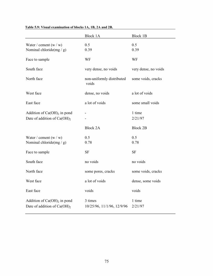
Table 5.9: Visual examination of blocks 1A, 1B, 2A and 2B.

Block 1A Block 1B

Water / cement (w / w) Nominal chloride(mg / g)

Face to sample

South face

North face

West face

East face

Addition of Ca(OH)2 in pond Date of addition of Ca(OH)2

Water / cement (w / w) Nominal chloride(mg / g)

Face to sample

South face

North face

West face

East face

Addition of Ca(OH)2 in pond Date of addition of Ca(OH)2

0.50.39

WF

very dense, no voids

non-uniformly distributedvoids

dense, no voids

a lot of voids

--

Block 2A

0.50.78

SF

no voids

some pores, cracks

a lot of voids

voids

3 times10/25/96, 11/1/96, 12/9/96

0.5 0.39

WF

very dense, no voids

some voids, cracks

a lot of voids

some small voids

1 time 2/21/97

Block 2B

0.5 0.78

SF

no voids

some voids, cracks

dense, some voids

voids

1 time 2/21/97

75

Table 5.9: (continued)

Block 3A Block 3B

Water / cement (w / w) Nominal chloride(mg / g)

Face to sample

South face

North face

West face

East face

Addition of Ca(OH)2 in pond Time period of addition of Ca(OH)2

Water / cement (w / w) Nominal chloride(mg / g)

Face to sample

South face

North face

West face

East face

Addition of Ca(OH)2 in pond Date of addition of Ca(OH)2

0.35 0.81

SF

very dense, no voids

a few voids, cracks

voids, dark gray spots

a few voids, dark gray spots

--

Block 4C

0.5 1.95

SF

very dense, no voids

non-uniformly distributed voids, cracks

a lot of voids

non-uniformly distributed voids

--

0.35 0.81

SF

dense, no voids

dense, no voids

very dense, a few voids

a lot of voids, dark gray spots

--

Block 4D

0.5 1.95

SF

dense, no voids

some voids, cracks

voids

voids

1 time 2/21/97

76

Sprayed zinc

Iron mesh

a)

b)

Figure 5.28: Distribution of pores in control block 4E: a) cutting of the cylinder; b) pictures of two sides of cut cylinder. Block dimensions: 15⋅15⋅15 cm, diameter of cylinder is 5 cm.

77

5.2.4.2 Chloride Profiles in Test Blocks

We were testing the hypothesis that, after long-term polarization, the chloride concentration would decrease in the vicinity of the steel mesh and increase near the zinc-mortar interface. The results of the tests carried out on the eight test blocks -- Figure 5.19, Figure 5.20, Figure 5.21, Figure 5.22, Figure 5.23, Figure 5.24, Figure 5.25 and Figure 5.26 -- exhibit considerable scatter, the majority of which is attributed to inhomogeneities in the blocks and associated sampling variability, and some of which is still unexplained. In any case, the data do not confirm the hypothesis. This result did not come as a surprise in view of the results of the modeling exercise presented in Section 2.3.

However, some of the data allow one to infer that migration has taken place, if one is predisposed to do so. Most pronounced in this regard are the profiles from blocks 4C (Figure 5.25, applied current density 0.066 A/m2, nominal chloride concentration 1.95 mg/g, w/c = 0.5) and 4D (Figure 5.26, applied current density 0.033 A/m2, nominal chloride concentration 1.95 mg/g, w/c = 0.5). These blocks did have the highest chloride concentrations and one would expect the greatest transference number for chloride in these blocks, and hence, the greatest change in chloride concentration. However, no features of the curves directly reflect the factor of two difference in current density between the two blocks. The other blocks are even less clear in the evidence for migration.

78

6.0 SUMMARY

This project was designed as a study of the migration of chloride ions in mortar as a function of the applied current, composition of the mortar, and time of polarization. The experimental work included preparation of the mortar blocks, development of the method for long-term polarization, and development of a method of chloride analysis for small samples of mortar. The conclusion of this study is that, although some evidence for chloride migration could be inferred from certain parts of the experimental data, the data set as a whole shows no convincing evidence for chloride migration for the conditions of the experiment. This result is consistent with a simple transport model of the system.

The scatter in the data for chloride in the concrete was much greater than expected and was attributed primarily to non-representativeness of the small samples that were taken. Although the preparation of mortar blocks was carried out according to the standard procedure, it was found that the majority of blocks were not uniform with respect to the distribution of chloride ion on the scale of the sample size. A possible reason for the nonuniformity is the presence of pores, which were not uniform in size and distribution, and which contained a nonrepresentative amount of chloride. Furthermore, the continuous hydration process might introduce some uncertainty in the distribution of chloride in mortar.

Pilot tests on the long-term polarization of mortar blocks revealed a large increase in resistivity at the zinc-mortar interface, which could be reversed by wetting of the interface. To overcome this problem in the long-term test, ponds with saturated calcium hydroxide solution were placed on top of zinc side of the blocks. An eight channel power supply was constructed to apply constant current to eight blocks simultaneously in the course of a long-term migration experiment.

Two methods of analysis of mortar for chloride were investigated in this project: double standard addition potentiometry and ion chromatography. It was found that the first technique was good in precision only when the mortar samples were filtered before measurements. Inclusion of the filtration step increased the time of analysis significantly (30 minutes per sample) and resulted in the rejection of the potentiometric method. The other method of chloride analysis, IC, was shown to work successfully for the determination of chloride in mortar and was used in the chloride migration study.

The absence of clear experimental evidence for migration precluded further quantitative characterization of transport processes and model development. Towards the goal of a quantitative understanding of transport processes in concrete, two recommendations can be made. First, the test blocks should be larger in size to allow larger and more representative mortar samples to be collected. Second, an automated method of wetting the surface should be incorporated in the test protocol to obviate the need for the ponds on the top of the blocks.

79

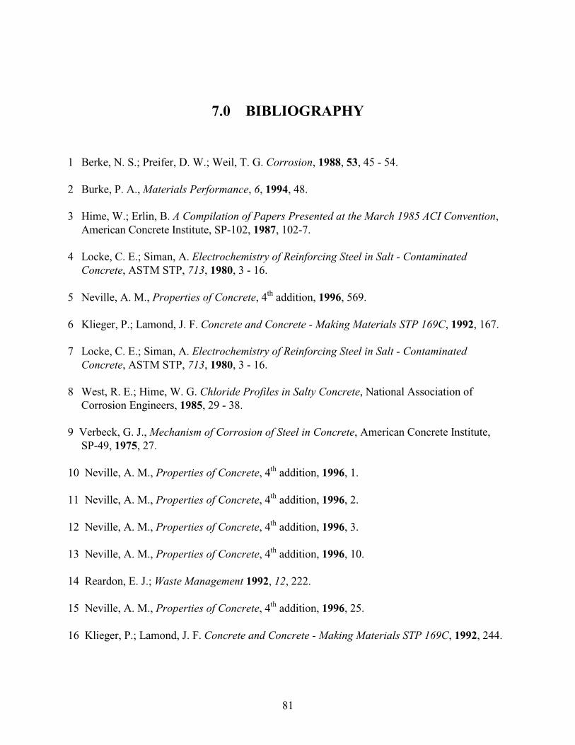
7.0 BIBLIOGRAPHY

1 Berke, N. S.; Preifer, D. W.; Weil, T. G. Corrosion, 1988, 53, 45 - 54.

2 Burke, P. A., Materials Performance, 6, 1994, 48.

3 Hime, W.; Erlin, B. A Compilation of Papers Presented at the March 1985 ACI Convention, American Concrete Institute, SP-102, 1987, 102-7.

4 Locke, C. E.; Siman, A. Electrochemistry of Reinforcing Steel in Salt - Contaminated Concrete, ASTM STP, 713, 1980, 3 - 16.

5 Neville, A. M., Properties of Concrete, 4th addition, 1996, 569.

6 Klieger, P.; Lamond, J. F. Concrete and Concrete - Making Materials STP 169C, 1992, 167.

7 Locke, C. E.; Siman, A. Electrochemistry of Reinforcing Steel in Salt - Contaminated Concrete, ASTM STP, 713, 1980, 3 - 16.

8 West, R. E.; Hime, W. G. Chloride Profiles in Salty Concrete, National Association of Corrosion Engineers, 1985, 29 - 38.

9 Verbeck, G. J., Mechanism of Corrosion of Steel in Concrete, American Concrete Institute, SP-49, 1975, 27.

10 Neville, A. M., Properties of Concrete, 4th addition, 1996, 1.

11 Neville, A. M., Properties of Concrete, 4th addition, 1996, 2.

12 Neville, A. M., Properties of Concrete, 4th addition, 1996, 3.

13 Neville, A. M., Properties of Concrete, 4th addition, 1996, 10.

14 Reardon, E. J.; Waste Management 1992, 12, 222.

15 Neville, A. M., Properties of Concrete, 4th addition, 1996, 25.

16 Klieger, P.; Lamond, J. F. Concrete and Concrete - Making Materials STP 169C, 1992, 244.

81

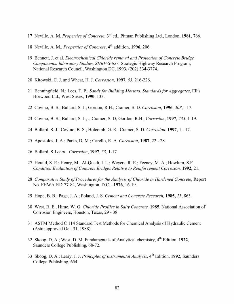
17 Neville, A. M. Properties of Concrete, 3rd ed., Pitman Publishing Ltd., London, 1981, 766.

18 Neville, A. M., Properties of Concrete, 4th addition, 1996, 206.

19 Bennett, J. et al. Electrochemical Chloride removal and Protection of Concrete Bridge Components: laboratory Studies. SHRP-S-657. Strategic Highway Research Program, National Research Council, Washington DC, 1993, (202) 334-3774.

20 Kitowski, C. J. and Wheat, H. J. Corrosion, 1997, 53, 216-226.

21 Benningfield, N.; Lees, T. P., Sands for Building Mortars. Standards for Aggregates, Ellis Horwood Ltd., West Susex, 1990, 133.

22 Covino, B. S.; Bullard, S. J.; Gordon, R.H.; Cramer, S. D. Corrosion, 1996, 308,1-17.

23 Covino, B. S.; Bullard, S. J.; .; Cramer, S. D; Gordon, R.H., Corrosion, 1997, 233, 1-19.

24 Bullard, S. J.; Covino, B. S.; Holcomb, G. R.; Cramer, S. D. Corrosion, 1997, 1 - 17.

25 Apostolos, J. A.; Parks, D. M.; Carello, R. A. Corrosion, 1987, 22 - 28.

26 Bullard, S.J et al. Corrosion, 1997, 53, 1-17

27 Herald, S. E.; Henry, M.; Al-Quadi, I. L.; Weyers, R. E.; Feeney, M. A.; Howlum, S.F. Condition Evaluation of Concrete Bridges Relative to Reinforcement Corrosion, 1992, 21.

28 Comparative Study of Procedures for the Analysis of Chloride in Hardened Concrete, Report No. FHWA-RD-77-84, Washington, D.C. , 1976, 16-19.

29 Hope, B. B.; Page, J. A.; Poland, J. S. Cement and Concrete Research, 1985, 15, 863.

30 West, R. E., Hime, W. G. Chloride Profiles in Salty Concrete, 1985, National Association of Corrosion Engineers, Houston, Texas, 29 - 38.

31 ASTM Method C 114 Standard Test Methods for Chemical Analysis of Hydraulic Cement (Astm approved Oct. 31, 1988).

32 Skoog, D. A.; West, D. M. Fundamentals of Analytical chemistry, 4th Edition, 1922, Saunders College Publishing, 68-72.

33 Skoog, D. A.; Leary, J. J. Principles of Instrumental Analysis, 4th Edition, 1992, Saunders College Publishing, 654.

82

34 Haddad, P.R.; Jackson, P. E. Journal of Chromatography Library, "Ion Chromatography.Principles and Applications", 1990, 46, 38.

35 Doury-Berthod, M.; Giampaoli, P.; Pitsch, H.; Sella, C.; Poitrenaud, C. Anal. Chem. 1985,57, 2257-2263.

36 Klieger, P.; Lamond, J. F. Concrete and Concrete - Making Materials STP 169C, 1992, 240.

83