The Structure of White Dwarf and Neutron Stars∗

David G. Robertson†

Department of Physics and Astronomy

Otterbein College, Westerville, OH 43081

(Dated: August 20, 2009)

Abstract

This module is an introduction to the physics of white dwarfs and neutron stars. The differential equations

that describe the equilibrium states of these objects are developed. An overview of techniques for the

numerical solution of ordinary differential equations is presented.

Keywords: white dwarf, neutron star, general relativity, Chandrasekhar limit, nuclear matter, equation of

state, ordinary differential equations, Euler method, Runge-Kutta method

∗ Work supported by the National Science Foundation under grant CCLI DUE 0618252.†Electronic address: drobertson@otterbein.edu

1

Contents

I. Module Overview 3

II. What You Will Need 3

III. Numerical Solution of Ordinary Differential Equations 4

A. Basic Concepts 4

B. More Accurate Techniques 7

C. The Runge-Kutta Algorithm 9

D. Exercises 10

IV. The Fates of the Stars 11

V. Equilibrium Equations and Grand Strategy 13

VI. White Dwarfs 15

A. Degenerate Fermi Gas Equation of State 16

B. Scaling the Equations 20

C. Exercises 21

D. Simulation Projects 22

VII. Neutron Stars 23

A. Relativistic corrections to the equilibrium equations 23

B. Degenerate neutron gas equation of state 24

C. Including nuclear interactions 25

D. Simulation Projects 26

VIII. Notes on Selected Exercises 27

A. Exercise III.D.4 27

B. Exercise VI.C.4 28

References 31

Glossary 33

2

I. MODULE OVERVIEW

This module is an introduction to the physics of white dwarfs and neutron stars, remnants left

behind by ordinary stars after they have ceased nuclear fusion. These objects support themselves

against gravitational collapse by physical mechanisms other than the pressure of hot gas (the

heat being generated by nuclear fusion at the core). A white dwarf is stabilized ultimately by

the “degeneracy pressure” of electrons arising from the Exclusion Principle. A neutron star is

stabilized mainly by repulsive strong interactions between the neutrons out of which it is (primarily)

composed.

The physics involved is extremely rich, involving gravitational physics (including general rela-

tivity in the case of neutron stars), thermodynamics, quantum mechanics, and nuclear and particle

physics. Exploring all aspects of this module will likely require considerable time, as well as a

solid grounding in all these topics. A great deal of flexibility is possible, however, in tailoring

the physics focus to match the student and instructor interests and backgrounds. Some portions

can be omitted entirely (e.g., neutron stars, or the development of the nuclear matter equation of

state), and in other cases needed relations can be motivated and then simply used, rather than

being derived in full.

The equilibrium structure of these objects is naturally described by a set of coupled ordinary

differential equations, which must be solved numerically. An overview of the relevant computational

techniques is also presented.

II. WHAT YOU WILL NEED

The minimal physics background required will include Newtonian gravity at the level of a

typical junior-level course in classical mechanics, thermodynamics, special relativity and quantum

mechanics at the introductory level, and, if neutron stars are to be explored, some nuclear and

particle physics, also at the introductory level. An upper-level course in quantum mechanics will be

helpful in clarifying some areas, as will additional exposure to thermodynamics. However, the basic

physical ideas should be accessible to the student who has mastered these minimal requirements.

The treatment of neutron stars brings in a number of advanced topics, particularly in nuclear

physics, where most of the relevant issues are the subjects of ongoing research efforts. An upper-

level course in nuclear and/or particle physics should allow a much deeper exploration of this

problem. The needed general relativity can be motivated using one of the excellent undergraduate-

3

level texts on the subject that have emerged recently [1, 2].

On the mathematical side, facility with differential and integral calculus is essential, as is a basic

familiarity with ordinary differential equations. Students who have passed through a junior-level

mechanics course should certainly have the necessary background.

The computing resources needed are actually minimal, as the “size” of the computational prob-

lem is rather modest. The natural framework for scientific computing is a high-level language like

Fortran, C or C++, and this is an excellent project for students to sharpen their programming

skills. However, the needed calculations can be done using Matlab or even with a spreadsheet such

as Excel. Some facility for generating plots will also be useful, for example Excel or gnuplot, and

access to Mathematica or Maple will greatly ease the analytical calculations in the exercises, as

well as the physics modeling for the nuclear equation of state.

III. NUMERICAL SOLUTION OF ORDINARY DIFFERENTIAL EQUATIONS

In this section I shall discuss the basics of solving ordinary differential equations on a computer.

A disclaimer is perhaps in order. This is actually a large and technical area, and we can afford to

touch only on the most basic aspects here. Knowledgeable readers may in fact find certain aspects

of the presentation to be scandalously slipshod and incomplete. In response I can only say that

my goal is to give a basic overview that illustrates most of the relevant issues. My hope is that

this orientation will be sufficient to help guide interested students in further inquiry, should they

choose to pursue it. Additional details may be found in, for example, refs. [3–5].

A. Basic Concepts

An ordinary differential equation (ODE) is an equation satisfied by a function of a single inde-

pendent variable, involving derivatives of that function. The order of the ODE is the order of the

highest derivative that occurs; thus

d3y

dx3+ a(x)

d2y

dx2+ b(x)

dy

dx+ c(x)y + d(x) = 0, (3.1)

where a, b, c and d are specified functions, is a third-order ODE for the function y(x). We may

also consider a system of ODEs that determines a set of functions, each of the same independent

variable. Typically each function appears in more than one of the equations, so that they are

coupled. Any equation involving only one of the functions can be solved independently of the

others.

4

To determine a unique solution to an n-th order ODE, it is necessary to further provide n

independent “boundary conditions,” or known values of the function and/or its derivatives for

some value(s) of the independent variable. Often this takes the form of specifying the function and

n − 1 of its derivatives at some common reference value of x; this is known as the “initial value

problem.” (For convenience we often choose this reference point to be x = 0, if possible.) The

canonical example would be the solution to Newton’s second law of motion, a second-order ODE.

A unique solution is determined by specifying the position and velocity at some reference time.

There are other possibilities as well for the specification of boundary values, but in this module I

shall focus on the initial value problem.

As a first step, note that an ODE of any order can always be reduced to a coupled system of

first-order ODEs. The basic point may be appreciated by considering Newton’s second law in one

dimension,

d2y

dt2= f(y), (3.2)

where f = F/m with F the net force and m the mass. This is a second-order ODE, but by

introducing the velocity v = dy/dt we can re-write it as a pair first-order equations:

dy

dt= v (3.3)

dv

dt= f(y). (3.4)

The idea is easy to generalize and we leave this to the reader. In general, an n-th order equation

will reduce to a set of n first-order equations. It is therefore sufficient to consider a set of coupled

first-order ODEs. These equations will have the general form

dyidx

= fi(x, y1, . . . , yn) i = 1, . . . , n, (3.5)

where the yi are the functions to be determined and the fi are given. A full solution to these also

requires the specification of boundary conditions on the functions yi. As discussed above, we will

here consider only the initial value problem. Starting values for all the yi are thus specified at

some common x, which we take to be x = 0 for convenience. The system of equations (3.5) then

determines the yi for any other value of x.

Our basic approach to finding approximate solutions will be to advance in x in small steps

of size ε, treating eqs. (3.5) as a set of difference equations. We thus evaluate the solution at a

discrete set of x values, xn = nε, where n = 0, 1, 2, . . . . The differential equations are re-written

5

by replacing differentials dx and dy with differences ∆x and ∆y. The result is a set of algebraic

equations for the change in the functions yi in each “step” of size ∆x ≡ ε.

As an example, consider Newton’s second law as presented in eqs. (3.4). The simplest approach

would be to approximate these as

∆yε

= v (3.6)

∆vε

= f(y), (3.7)

whence

∆y = y(t+ ε)− y(t) = εv (3.8)

and

∆v = v(t+ ε)− v(t) = εf(y). (3.9)

Given values for y and v at time t, we can then obtain these quantities at the next step:

y(t+ ε) = y(t) + εv (3.10)

v(t+ ε) = v(t) + εf(y). (3.11)

The new values then allow us to take the next step, and so on. Since by assumption we have the

starting values for y and v at t = 0, we can step along and calculate y and v for any t. If ε is small

enough then the differences will approximate the differentials reasonably well, and the resulting

solution can be made as accurate as desired.

This approach, in which we approximate the original derivatives as

dy

dx≈ y(x+ ε)− y(x)

ε, (3.12)

is known as Euler’s method. It is the simplest approach to solving ODEs numerically, although it

is not especially accurate. To quantify the accuracy, let’s imagine we know the full solution y(x)

for all x. We can then Taylor expand around a point x to obtain

y(x+ ε) = y(x) + εy′(x) +O(ε2), (3.13)

where y′ = dy/dx as usual. We thus see that Euler’s method is equivalent to neglecting terms of

order ε2 (and higher) in the true answer. In principle this error can be made as small as we like,

however, by making ε sufficiently small [12].

6

However, the smaller we make ε, the more steps we need to take to obtain the solution at some

fixed x of interest. For simplicity, say we need y at x = 1. The number of steps needed is then

N = 1/ε. If the error in each step is O(ε2) then the total error in reaching x = 1 is NO(ε2) or

O(ε). Hence to make the solution twice as accurate we will need to halve the step size ε, leading

to twice as much computational work. The work involved is a single evaluation of the function f

at each step.

While conceptually simple, Euler’s method is not recommended for practical applications due

to its poor accuracy. In addition to the extra computational work required, the need to take many

steps to achieve high accuracy can magnify the effect of “roundoff error” in the computations.

The basic issue here is that real numbers are represented discretely on a computer, which means

that only a finite subset of all the reals actually “exist” on the computer. For example, say we

use a computer on which a float is 4 bytes, or 32 bits. Each bit can be 0 or 1, so there are

232 ≈ 4.3 × 109 possible different configurations of these bits. Thus the computer can at most

represent this many different floats from among the infinity of real numbers. The result is that

a float on the computer generally is slightly different than its “true” value – most of the “true”

values are simply not representable. Even if we do start with values that are represented exactly on

the computer, when we operate on them – multiply them together, for example – the exact result

is generally not represented. Thus a small error, called “roundoff error,” is unavoidably introduced

[13].

Often this roundoff error can be thought of as a sort of random error – it’s just as likely to

be positive as negative – so that it grows like√N for N calculations. In unfavorable cases the

situation may well be worse, however, and in very unfavorable situations this error may quickly

come to dominate a calculation. We will see an example of this below.

B. More Accurate Techniques

We would like to develop algorithms for solving our ODEs that have better accuracy than

Euler’s method, i.e., with overall errors that are O(εn) with n > 1. Such an algorithm will result

in a more rapid increase in accuracy with decreasing step size, leading to greater overall accuracy

for a fixed amount of computational work.

The invocation of the Taylor series above may suggest some ideas. For example, let us include

the next term in the expansion,

y(x+ ε) = y(x) + εy′(x) +12ε2y′′(x) + . . . . (3.14)

7

Since y′(x) = f(x, y) is a known function, we can calculate the second derivative in the ε2 term:

y′′(x) =df

dx

=∂f

∂x+∂f

∂y

dy

dx

=∂f

∂x+∂f

∂yf.

So we could step y using

y(x+ ε) = y(x) + εy′(x) +12ε2[∂f

∂x+ f

∂f

∂y

], (3.15)

which is correct to O(ε3). The overall error in taking n steps would then be O(ε2). This approach

is most useful when f is sufficiently simple that its derivatives can be readily computed.

As another example, consider that Euler’s method amounts to approximating the derivative

dy/dx by the “forward” difference:

dy

dx≈ y(x+ ε)− y(x)

ε. (3.16)

There is no reason to suppose this is any more accurate than the “backwards” difference

dy

dx≈ y(x)− y(x− ε)

ε, (3.17)

but consider using the average of these, the “symmetric” difference. In this case we would have

dy

dx≈ 1

2

[y(x+ ε)− y(x)

ε+y(x)− y(x− ε)

ε

]=

y(x+ ε)− y(x− ε)2ε

, (3.18)

resulting in

y(x+ ε) = y(x− ε) + 2εf(x, y). (3.19)

At first glance this looks about as good as Euler, but if we insert the Taylor expansions for y(x+ ε)

and y(x− ε) we find that all the O(ε2) terms on the right hand side of eq. (3.19) actually cancel;

hence this formula is accurate to O(ε3), as is eq. (3.15). We might even be tempted to use it in

preference to eq. (3.15), since it does not require us to take additional derivatives of f . However,

this approximation has a problem, which you can explore in one of the exercises. Do not use it to

solve a real problem!

8

C. The Runge-Kutta Algorithm

A very useful algorithm is known as the Runge-Kutta approach. It is stable and can be made

quite accurate, although it is not always the most efficient algorithm (i.e., the fastest for a given

accuracy). We shall derive here the second-order version of the RK algorithm, and then simply

present the more accurate fourth-order version.

We begin by observing that the basic Euler method,

y(x+ ε) = y(x) + εf(x, y), (3.20)

assumes the entire change in y over the step is obtained from the derivative at the beginning of the

step. (In fact, if the derivative is constant over the step, or in other words if y is a linear function

of x, then Euler’s methods is exact.) A better result might be obtained if we use eq. (3.20) to

take a “trial” step to the midpoint of the interval (x+ ε/2), and then take the full step from x to

x+ ε/2 using the midpoint values. This corresponds to using the (approximate) average derivative

over the interval in Euler’s method.

Specifically, we take for the trial step:

y(x+ ε/2) = y(x) + (ε/2)f(x, y), (3.21)

and then step from x to x+ ε using the midpoint values of both x and y:

y(x+ ε) = y(x) + εf(x+ ε/2, y(x+ ε/2)). (3.22)

This algorithm is more conventionally expressed by defining the quantities

k1 = εf(x, y) (3.23)

k2 = εf(x+ ε/2, y(x) + k1/2), (3.24)

and then stepping as

y(x+ ε) = y(x) + k2 +O(ε3). (3.25)

As indicated, the second order dependence on ε cancels (again, substitute the full Taylor expansions

into the given formulas to demonstrate this) so that the algorithm is accurate to O(ε3). The full

error in taking n steps will then be O(ε2), and hence this is known as the second-order Runge-Kutta

algorithm.

9

More accurate versions of this are possible, in which we take various partial steps across the

interval and combine them so that error terms of higher and higher order are cancelled. The most

popular version is probably the standard fourth-order algorithm, which is as follows:

k1 = εf(x, y) (3.26)

k2 = εf(x+ ε/2, y(x) + k1/2) (3.27)

k3 = εf(x+ ε/2, y(x) + k2/2) (3.28)

k4 = εf(x+ ε, y(x) + k3) (3.29)

y(x+ ε) = y(x) +k1

6+k2

3+k3

3+k4

6+O(ε5). (3.30)

It is a straightforward if somewhat tedious exercise to verify that all error terms through O(ε4)

cancel in eq. (3.30).

D. Exercises

1. Consider the equation

dy

dx= −xy

with initial condition y(0) = 1, which has the exact solution y = exp(−x2/2). Study the

numerical integration of this using the methods described above. In particular, verify that the

errors (difference between numerical and exact solutions) decrease according to the expected

power of ε.

2. Generalize one or more of the schemes presented here to solve a system of two coupled ODEs,

and apply it to solve Newton’s second law for the simple harmonic oscillator (with m = 1):

dx

dt= v

dv

dt= −ω2x.

A useful criterion for accuracy is the degree to which a known integral of the motion, for

example, the energy, is conserved in the evolution. Study the constancy of 2E = v2 + ω2x2

for the various algorithms and choices for ε.

3. Another common test of accuracy is to integrate backwards to the original starting point,

using the ending x, y as the initial condition. The difference between the resulting value for

10

y and the original initial condition then gives a measure of the overall accuracy of the result.

Apply this test to the example from problem 1, for the various algorithms discussed above.

4. Study the approximation given in eq. (3.19), by using it to solve the equation

dy

dx= −y,

with the initial condition y(0) = 1. This equation has the exact solution

y = e−x,

of course. To start the calculation off we need both y(0) and y(ε); you can use eq. (3.15) to

obtain y(ε). Eq. (3.19) can then be used to generate the solution for other values of x. Does

this give a reasonable approximation to the exact answer? If not, can you determine why?

See the notes in sec. VIII.A for further discussion of this example.

IV. THE FATES OF THE STARS

The structure of stars, their evolution from birth to death, and the remnants they leave behind

are central problems in astrophysics. The basics of star formation are well described in a number

of introductory astronomy texts, and the reader may wish to consult one of these to “set the stage”

[6]. Here we shall focus on the end of a star’s life.

Stars in their prime, while they are on the “main sequence,” support themselves against gravi-

tational collapse by the pressure of hot gas, the energy being released in nuclear fusion reactions at

the star’s core. For most of its life, the fusion reactions are dominated by protons (hydrogen nuclei)

fusing to form helium nuclei, the same process that powers thermonuclear weapons on Earth.

The helium nuclei are harder to involve in fusion reactions than protons: they have a greater

electric charge and thus experience greater repulsion from other nuclei in their vicinity. However,

if the star is sufficiently massive, so that the inward pressure of gravity is high enough, this barrier

can be overcome and the helium made to fuse into heavier nuclei, with additional energy release.

And so, given a sufficiently large star, it works its way up the periodic table, creating heavier and

heavier nuclei so long as the core pressure and temperature can rise high enough.

But at some point the nuclear reactions will cease. This can happen for a couple of reasons,

depending ultimately on the total mass of the star. First, the star may not be big enough to

continue driving fusion reactions past some point; in this case, a non-burning “ash” of the last

nucleus produced will build up in the core of the star. The details of what happens next are

11

complicated, but essentially the fusion shuts down and the star is unable to produce the energy

it needs to resist gravitational collapse. It therefore collapses, and the question is whether some

other force or mechanism can intervene to halt this collapse.

A second possibility arises if the star is very large, large enough to drive the fusion all the way

to 56Fe. In this case nuclear physics intervenes, for further fusion does not produce energy at all,

but rather absorbs it. The effect is thus to act as a sort of “fire extinguisher,” cooling the core and

eventually shutting off further nuclear reactions. The end result is the same as above: the star can

no longer support itself against gravitational collapse.

So now what happens? At this stage the star is composed of a variety of nuclei, i.e. protons and

neutrons, as well as a number of electrons equal to the total number of protons. It is collapsing. If

there is not a non-thermal source of pressure that can stabilize it, it will collapse to a very small

size, becoming a black hole. Black holes are often described loosely as being objects so massive

that not even light can escape, but it is perhaps more accurate to say that they warp spacetime

so severely in their vicinity that they create a sort of “knot,” in which there is simply no direction

you (or a light ray) can travel that takes you away from it.

This is the inevitable fate of stars that are sufficiently large, but for low- to mid-range stars there

are two other basic possibilities, again depending on the mass. If the mass is not too large, then the

“degeneracy pressure” of the electrons can stabilize it against further collapse; the result is known as

a white dwarf. This is an effect of the Pauli Exclusion Principle, which states that no two electrons

(or other fermions) can be in the same quantum state. The result is that, roughly speaking, the

electrons cannot get too close to each other (note that this is not a result of Coulomb repulsion!),

and there is effectively a sort of pressure that resists further compression of the electrons.

However, if the mass is sufficiently large then this electron degeneracy pressure is unable to

support the star and the collapse continues. Eventually the protons and electrons are so close

together that they undergo inverse beta decay, combining to produce neutrons (and neutrinos,

which quickly escape the star). The star becomes composed almost entirely of neutrons. At

this point the strong nuclear force can perhaps stabilize the star, for there is ultimately a strong

repulsive force between neutrons this close together. If this occurs the result is known as a neutron

star.

In what follows we will study the global properties of white dwarfs and neutron stars, deter-

mining the relation between mass and radius that follows from requiring equilibrium between the

inward pull of gravity against the electron degeneracy pressure or neutron repulsion, respectively.

12

P(r +dr)dA

P(r)dA

dV

r +dr

r

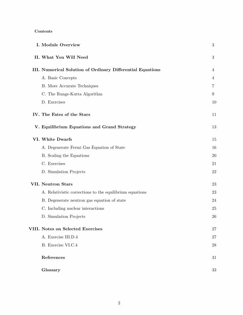
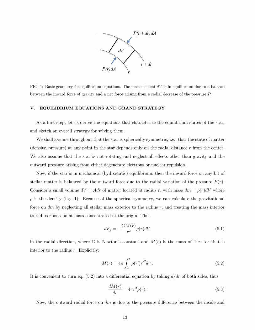
FIG. 1: Basic geometry for equilibrium equations. The mass element dV is in equilibrium due to a balance

between the inward force of gravity and a net force arising from a radial decrease of the pressure P .

V. EQUILIBRIUM EQUATIONS AND GRAND STRATEGY

As a first step, let us derive the equations that characterize the equilibrium states of the star,

and sketch an overall strategy for solving them.

We shall assume throughout that the star is spherically symmetric, i.e., that the state of matter

(density, pressure) at any point in the star depends only on the radial distance r from the center.

We also assume that the star is not rotating and neglect all effects other than gravity and the

outward pressure arising from either degenerate electrons or nuclear repulsion.

Now, if the star is in mechanical (hydrostatic) equilibrium, then the inward force on any bit of

stellar matter is balanced by the outward force due to the radial variation of the pressure P (r).

Consider a small volume dV = Adr of matter located at radius r, with mass dm = ρ(r)dV where

ρ is the density (fig. 1). Because of the spherical symmetry, we can calculate the gravitational

force on dm by neglecting all stellar mass exterior to the radius r, and treating the mass interior

to radius r as a point mass concentrated at the origin. Thus

dFg = −GM(r)r2

ρ(r)dV (5.1)

in the radial direction, where G is Newton’s constant and M(r) is the mass of the star that is

interior to the radius r. Explicitly:

M(r) = 4π∫ r

0ρ(r′)r′2dr′. (5.2)

It is convenient to turn eq. (5.2) into a differential equation by taking d/dr of both sides; thus

dM(r)dr

= 4πr2ρ(r). (5.3)

Now, the outward radial force on dm is due to the pressure difference between the inside and

13

outside,

dFp = P (r)A− P (r + dr)A, (5.4)

where A is the area over which the radial pressure acts. Since

P (r + dr) = P (r) +dP

drdr + · · · (5.5)

we have, to first order in dr,

dFp = P (r)A−[P (r) +

dP

drdr

]A

= −dPdrdV. (5.6)

In equilibrium we must have dFp + dFg = 0, so that

dP (r)dr

= −GM(r)ρ(r)r2

. (5.7)

This relation, along with eq. (5.3), which supplies the connection between ρ and M , is our first

equation defining the equilibrium state of the star.

Before proceeding, let us note that the Newtonian formula (5.1) is adequate so long as the

gravitational field is not too strong, or, in the language of general relativity, the spacetime curvature

is not too large. Such is the case for white dwarfs, as we shall verify later. However, for more

compact objects, such as neutron stars, relativistic effects become important. We will discuss these

in due course.

Eq. (5.7) is one relation involving two unknowns, P and ρ. (Remember that M is given in

terms of ρ by eq. (5.3).) A second relation between P and ρ is known as the “equation of state”

for the star; it expresses the properties of the matter making up the star. We will explore a variety

of models leading to different equations of state, but for now let us imagine we have such a relation

P = P (ρ) and discuss how we will solve the various equations to determine the stellar structure.

Given P = P (ρ) we can use the Chain Rule to write

dP

dr=dP

dρ

dρ

dr, (5.8)

where dP/dρ can be calculated. Using this we can eliminate the pressure in eq. (5.7), obtaining

dρ

dr= −

(dP

dρ

)−1 GM(r)ρ(r)r2

. (5.9)

Equations (5.9) and (5.3) are then a pair of coupled first-order ODEs involving only ρ(r) and M(r).

14

To solve them, we can integrate them from r = 0, with the initial conditions M(0) = 0 and

ρ = ρc, some specified central density. The integration gives the density profile ρ(r) of the star

as well as M(r). At some radius R the density ρ will drop to zero; this is taken to be the edge

of the star. In this way we can determine the radius and total mass M(R) of the equilibrium

configurations. Since both R and M depend on ρc, variation of this parameter allows stars of

different masses to be studied.

Let us now seek an equation of state appropriate for a white dwarf. Later we will consider

neutron stars.

VI. WHITE DWARFS

As discussed above, a white dwarf consists of heavy nuclei (protons and neutrons, here assumed

to have the same mass mN ) and electrons, and it is the electron degeneracy pressure which ul-

timately stabilizes the star against collapse. The densities inside a white dwarf are much higher

than in ordinary matter, and the electrons are not bound to nuclei; rather, they are quasi-free and

travel throughout the star. Since they are much lighter than the nuclei (mN/me ' 1800) they

move around more and produce most of the pressure. On the other hand, the nuclei provide most

of the mass of the star.

We shall treat the nuclei as essentially static, providing the entire mass of the star through

their rest mass. The electrons constitute a sort of gas, called a “degenerate Fermi gas,” since the

electrons are fermions. In this context, “degenerate” indicates the electrons are in their ground

state. The Exclusion Principle forces the electrons to fill a “Fermi sea,” a tower of states with

increasing energy, much like the atomic orbitals of the elements. The result is that the electrons

necessarily move about, thereby producing pressure in the star.

We can make a simple estimate of the maximum mass of a white dwarf that exposes most of

the basic physical ideas, using an argument given originally by L.D. Landau [7]. Let us imagine

the star to be a sphere of radius R, composed of N electrons and N protons. The protons supply

most of the mass, so the gravitational potential energy of the system is roughly

Eg ∼ −G(NmN )2

R, (6.1)

where mN is the nucleon mass. The N electrons occupy a volume ∼ R3; since they cannot overlap

(by the Exclusion Principle), each occupies a volume ∼ R3/N in size. The characteristic length

associated with their wavefunctions is then λ ∼ R/N1/3. If we take this to be the typical de Broglie

15

wavelength of the electrons, then they have a characteristic momentum

p =h

λ∼ hN1/3

R. (6.2)

From this we see that as we reduce R, the energy of the electrons increases as they are forced to

occupy a smaller volume. Thus we must do positive work to compress the electrons.

For simplicity let’s assume the electrons are highly relativistic, so their energy is given by

E =√p2c2 +m2

ec4 ' pc. (6.3)

The total energy of electrons in the star is then roughly

Ee ∼ Npc =hcN4/3

R, (6.4)

and the total energy of the star is

E ∼ −G(mNN)2

R+hcN4/3

R. (6.5)

Now the point is that the first term increases more rapidly than the second with increasing N .

Hence as N increases the first term will eventually come to dominate and the total energy will

become negative; in this case the star will find it energetically favorable to collapse to a very small

size R ∼ 0. The critical value of N for which this happens is about

Nmax ∼(

hc

Gm2N

)3/2

. (6.6)

Plugging in the values for the various constants we obtain

Nmax ∼ 1058, (6.7)

corresponding to a total mass

Mmax = NmaxmN ∼ 10M�. (6.8)

This upper limit on the mass of a white dwarf is known as the Chandrasekhar mass [8]. We will

now develop the machinery for a more accurate calculation.

A. Degenerate Fermi Gas Equation of State

Let’s begin by establishing some notation. We assume the entire mass of the star is due to the

rest mass of the nucleons, hence the mass density can be written as

ρ = nNmN , (6.9)

16

where nN is the number density of nucleons. If we define α to be the number of electrons per

nucleon in the star, then the electron number density n is given by

n = αnN

=αρ

mN. (6.10)

The parameter α is the same as the fraction of nucleons that are protons, since the star as a whole

is electrically neutral (i.e., has the same number of electrons and protons). Thus if the nuclei are

all 12C (6 protons and 6 neutrons) then α = 0.5.

Now imagine we have a collection of N electrons in a large volume V at zero temperature. At

zero temperature the electrons will settle into the ground state, i.e., the state with the lowest total

energy. Our plan for computing the pressure is as follows. First we will calculate the total energy

E of the electrons. This is obtained by filling the quantum energy levels for the electrons in accord

with the Exclusion Principle, and then adding up the energies of these electrons. We can then

compute the pressure P from

P = −∂E∂V

, (6.11)

with the number of electrons held fixed. It is reasonable to consider the electrons as free (i.e., non-

interacting) since they move in an essentially uniform neutral background of the other electrons

and protons. They therefore see very little effective charge, on average, and their potential energy

can be neglected. To explore why it is reasonable to take the temperature of the electron gas to

be zero, despite the fact that the surface temperature of a white dwarf can be as high as ∼ 105 K,

see the exercises.

Since the electrons are essentially free, their wavefunctions are simple plane waves in a volume

V , that is, infinite square well wavefunctions. Consider the one-dimensional case, for simplicity,

and for now assume the electrons are non-relativistic. The energy levels are then given by

En =n2h2

8mL2, n = 1, 2, . . . (6.12)

where L is the length of the box. This is just p2n/2m, the non-relativistic kinetic energy, with

pn = nh/2L, the de Broglie momentum.

Now imagine filling these states with N electrons so that we get the lowest total energy [14].

We start by filling the lowest (n = 1) state with two electrons, one for each spin projection, then

the n = 1 level, and so on until all N electrons have been added. The total energy of the system

17

is then

E = 2N/2∑n=1

En, (6.13)

where the factor 2 accounts for the two spin states in each level. The magnitude of the largest

momentum that occurs in the sum is known as the Fermi momentum, usually denoted pf . Thus

pf = (N/2)h/2L = Nh/4L here.

When N is very large, as is the case for macroscopic matter including the stars we are discussing,

sums such as appear in (6.13) can be well approximated by integrals. The basic tool for making

this transition is the “density of states,” the number of states available to the particles in a small

momentum range. This is derived in most introductory books on quantum mechanics, and we refer

the reader to one of these for details. The result (in three dimensions) is that the number of states

with momentum components in the range (px, py, pz) to (px + dpx, py + dpy, pz + dpz) is

2Vd3p

(2πh̄)3, (6.14)

where d3p ≡ dpxdpydpz. The factor of two here again reflects the two distinct spin states allowed

by the Exclusion Principle for each value of the momentum. We would then re-write eq. (6.13) as

the integral

E = 2V∫ pf

0

d3p

(2πh̄)3E(p), (6.15)

where E(p) is the energy of a single particle with momentum p. Note that the integration limits

have been written in terms of the magnitude of the momentum. Similarly, the total number of

electrons is given by

N = 2V∫ pf

0

d3p

(2πh̄)3. (6.16)

Evaluating this integral gives

N = 2V∫ pf

0

4πp2dp

(2πh̄)3

= (2V )4πp3

f

3(2πh̄)3. (6.17)

The number density of electrons is then

n =N

V=

p3f

3π2h̄3 . (6.18)

This gives the Fermi momentum in terms of n:

pf = h̄(3π2n)1/3. (6.19)

18

One should think of the Fermi momentum pf as a proxy for the density n.

Next let us calculate the total energy. We shall treat the electrons relativstically, so for the

energy we take

E(p) =√p2c2 +m2c4. (6.20)

The total energy is then

E = 2V∫ pf

0

d3p

(2πh̄)3√p2c2 +m2

ec4. (6.21)

Remember that pf is a function of n, so this gives a relation between E and n, which is just what

we want. This integral is not too difficult to evaluate, but it is simple in the non-relativistic limit,

where E(p) ≈ mec2 + p2/2m, and in the extreme relativistic limit, where E(p) ≈ pc. Here I will

work out the latter case in detail, leaving the others to the exercises.

In the extreme relativistic limit we have

E = 2V∫ pf

0

4πp2dp

(2πh̄)3pc =

V cp4f

4π2h̄3 . (6.22)

Expressing this in terms of n using eq. (6.19) we find

E =3V4h̄c(3π2)1/3n4/3. (6.23)

Next we compute the pressure, using eq. (6.11). We find

−P =(∂E

∂V

)N

= an4/3 +4aV

3n1/3 dn

dV, (6.24)

where a = (3/4)(3π2)1/3h̄c. Since n = N/V we have

dn

dV= − N

V 2= − n

V, (6.25)

so that

−P = an4/3 − 43an4/3

= −13an4/3. (6.26)

Hence the equation of state is

P =14

(3π2)1/3h̄cn4/3 (6.27)

19

for highly relativistic electrons. Such a power law equation of state (i.e., P ∝ ργ) is known as a

polytrope.

Finally, we can calculate dP/dρ, for use in eq. (5.9). We first express P in terms of ρ, using eq.

(6.10):

P =14

(3π2)1/3h̄c(

α

mN

)4/3

ρ4/3, (6.28)

whence

dP

dρ=

13

(3π2)1/3h̄c(

α

mN

)4/3

ρ1/3. (6.29)

This can now be inserted into eq. (5.9) to give the desired equation involving ρ(r) and M(r):

dρ

dr= − 3G

(3π2)1/3h̄c

(mN

α

)4/3 M(r)ρ2/3(r)r2

. (6.30)

Along with eq. (5.3), we now have our set of coupled first-order differential equations for ρ(r) and

M(r).

B. Scaling the Equations

For numerical work it is useful to rescale the variables involved to that their actual numerical

values are neither too large nor too small. (Computer arithmetic with extremely large or small

numbers is more subject to inaccuracy.) To this end we introduce dimensionless variables r, ρ and

M :

r = R0r, ρ = ρ0ρ, M = M0M, (6.31)

where R0, ρ0 and M0 are constants chosen for convenience. We will take ρ0, somewhat arbitrarily,

to be the density when the electron Fermi momentum is equal to the electron mass (times c):

ρ0 =n0mN

α(6.32)

with

n0 =m3ec

3

3π2h̄3 . (6.33)

This density is characteristic of the electron gas intermediate between the non-relativistic (pf �

mec) and highly relativistic (pf � mec) regimes.

20

Plugging definitions (6.31) into eqs. (5.9) and (5.3), we then obtain, after some rearrangement,

dM

dr=[

4πR30ρ0

M0

]r2ρ (6.34)

dρ

dr= −

[3GM0

R0ρ1/30 (3π2)1/3h̄c

(mN

α

)4/3]M ρ2/3

r2. (6.35)

Now let us choose R0 and M0 so that the factors in square brackets are each equal to one. This

gives, eliminating M0 in favor of R0 and ρ0,

R0 =

[(3π2)1/3h̄c

12πG

(α

mN

)4/3 1

ρ2/30

]1/2

. (6.36)

Then, once ρ0 and R0 are known, we can calculate

M0 = 4πR30ρ0. (6.37)

The dimensionless differential equations are thus

dM

dr= r2ρ (6.38)

dρ

dr= −M ρ2/3

r2. (6.39)

Once the solutions are obtained for M and R, we multiply by M0 and R0, respectively, to restore

the physical units.

C. Exercises

1. White dwarfs may have surface temperatures of 105 K. Why is it reasonable to treat the

electron gas as degenerate, i.e., effectively at zero temperature (and hence in its ground

state)?

2. Obtain the numerical values in MKS units for ρ0, M0 and R0.

3. Evaluate the electron pressure and equation of state in the non-relativistic limit, i.e., assum-

ing p� me for all electrons.

4. Evaluate the electron pressure and equation of state in the general case, i.e., using the full

relativistic expression for the electron energies. Details of this calculation are given in section

VIII.B.

21

5. Recall that our plan is to integrate numerically equations (6.38) and (6.39) starting at r = 0,

with initial conditions M = 0 and ρ = ρc. Right away a complication arises, however: we

cannot use r = 0 to take the first step. (See the factor r2 in the denominator of eq. (6.39).

Also, M will never change from zero!) Here are a couple of ways of dealing with this.

(a) We can just start a short distance away from r = 0, say at r = ε. The simplest way to

do this in practice is just to stipulate that ρc is not quite the central density, but rather

then density at r = ε. For consistency, then, the starting M is not zero. What should

we take for M(ε)? You should assume that ε is sufficiently small that ρ is effectively

constant over this range.

(b) Alternatively, we can continue to take ρc to be the central density and work out how all

these quantities change in response to a small step in r. Then we can take the first step

“manually,” using the differential equations to continue on once r 6= 0. To implement

this, imagine Taylor expanding ρ and M in powers of r. For small r these will look like

M = αra + · · · (6.40)

and

ρ = ρc − βrb + · · · (6.41)

where α, a, β and b are constants, and the dots represent higher powers in r (which can

be neglected for small r). Determine the constants by plugging these into the equations

(6.38) and (6.39) and equating powers of r. Then use your results to calculate ρ and

M a short distance away from the origin.

D. Simulation Projects

Write a program to solve the equations (6.38) and (6.39). As discussed previously, the idea is

to numerically integrate these starting at r = 0 with the initial conditions M = 0 and ρ = ρc. The

radius R of the white dwarf is the value of r at which ρ = 0, and M(R) is the total mass at this

point.

Once you have the simulation working, calculate the total masses and radii of white dwarfs

with ρc values ranging from about 10−1 to 106. This gives a family of equilibrium configurations.

By changing the integration step and (maybe) the algorithm used, verify that your solutions are

accurate.

22

A useful way to display these results is as a plot of radius versus mass. Can you identify the

point at which the star can no longer be supported by degenerate electrons? This limiting mass

for white dwarfs (with α = 0.5) is known as the Chandrasekhar mass. Calculate its value in units

of the mass of the sun.

If you have time, explore the validity of the various approximations used in deriving the equation

of state. Is it more appropriate to treat the electrons as highly relativistic or non-relativistic? If

you have worked out the general case (exercise VI.C.4), compare the limiting mass obtained from

this to that obtained from one or more of the approximate forms.

Finally, vary the composition of the star from 12C to 56Fe, and study the variation in maximum

mass, radius, etc.

VII. NEUTRON STARS

The treatment of neutron stars is similar, although it involves some more exotic physics. For

one thing, neutron stars are so dense and create such strong gravitational fields (or spacetime

curvature, in the language of general relativity) that the differences between Newtonian gravity

and general relativity become noticeable. Relativistic corrections to the equilibrium equations are

significant and must be included to obtain a reasonable description.

In addition, as discussed above, the neutrons of which the star is mostly composed are com-

pressed to a very high density, perhaps 5-10 times the density found in ordinary nuclei. The

properties of matter in this extreme state are not well understood, due to the critical influence

of the strong nuclear force. Hence the correct equation of state is rather uncertain. This is a

subject of ongoing research efforts, with equations of state based on various models of the strong

interaction giving a fairly wide range of neutron star properties.

We shall begin by presenting the relativistic corrections to the structure equations. An overview

of possible equations of state then follows.

A. Relativistic corrections to the equilibrium equations

A derivation of the leading corrections to eq. (5.1) arising from special and general relativity is

beyond the scope of this project. Interested readers may consult one of the standard references on

the subject [9]. The result is known as the Tolman-Oppenheimer-Volkov (TOV) equation:

dP (r)dr

= −GM(r)ε(r)c2r2

[1 +

P (r)ε(r)c2

] [1 +

4πr3P (r)M(r)c2

] [1− 2GM(r)

c2r

]−1

. (7.1)

23

Note that I have renamed ρ→ ε/c2, to emphasize that it is an energy density. In the white dwarf

case the density was well accounted for by the rest mass of nucleons only, but for neutron stars

the kinetic and potential energies of the neutrons will make significant contributions to the total

energy. In relativistic physics mass and energy are equivalent, and in particular in general relativity

it is mass-energy that causes spacetime curvature.

To include relativistic corrections in the problem we simply include the three factors in square

brackets from eq. (7.1) on the right hand side of (5.9). For the record, the first two terms in

square brackets are special relativistic corrections, while the third arises from general relativity

[15]. Equation (5.3) does not change, apart from the renaming ρ→ ε/c2:

dM(r)dr

=4πr2ε(r)

c2. (7.2)

The total mass of the star includes all sources of internal energy, including neutron interaction

energy.

B. Degenerate neutron gas equation of state

We next consider the equation of state for nuclear matter. The simplest approach, taken in the

original calculations of neutron star structure [10], is just to treat the nuclear matter as a degenerate

gas of neutrons. This may be suspect because it ignores the strong nucleon-nucleon interaction,

which makes a sizable contribution to the energy (and hence the pressure). It is straightforward

to implement, however, using the machinery developed for white dwarfs. We simply replace the

electron mass me by mN .

As a refinement, we can incorporate the fact that the neutron star actually has a small admixture

of protons (and an equal number of electrons, to maintain charge neutrality). This is because the

neutrons undergo spontaneous beta decay

n→ p+ e− + νe. (7.3)

Of course, the inverse reaction

p+ e− → n+ νe (7.4)

is also proceeding and the result is to establish an equilibrium of rates (detailed balance) with a

steady state proportion of protons.

This rate equilibrium is expressed by a relation between chemical potentials

µn = µp + µe. (7.5)

24

(The neutrinos do not contribute (µν ≈ 0) since they escape from the star with essentially no

interaction; this is in fact the dominant mechanism whereby the neutron star loses energy and

cools.) With

µi =dεidni

(i = n, p, e−) (7.6)

we find, for a degenerate Fermi gas,

µi = (p2f,i +m2

i )1/2. (7.7)

(I am using units with c = 1 to avoid clutter.) Now, the star is electrically neutral so the proton

and electron densities are equal. Hence their Fermi momenta are the same: pf,e = pf,p. The

condition for equilibrium then becomes

(p2f,n +m2

n)1/2 = (p2f,p +m2

p)1/2 + (p2

f,p +m2e)

1/2 (7.8)

(note that we must now use the actual proton and neutron masses!). This relation can be solved

to give the proton Fermi momentum in terms of pf,n:

pf,p =

[(p2f,n +m2

n −m2e)

2 − 2m2p(p

2f,n +m2

n +m2e) +m4

p

]1/22(p2

f,n +m2n)1/2

. (7.9)

We can now use this to incorporate protons and electrons into the simulation. The energy (and

hence pressure) receive contributions from all three species of particle:

ε =∑

i=n,p,e−

εi, (7.10)

where the individual contributions all take the form of eq. (6.21). The simulation proceeds by

tracking the neutron density; at each step we use eq. (7.9) to calculate the proton and electron

densities. When the neutron density drops to zero the edge of the star is reached.

C. Including nuclear interactions

As discussed previously, in a neutron star the interaction energy of the neutrons is an important

component of the total energy, unlike in the case of degenerate electrons. Since energy is mass

(relativity is important here!) it must be accounted for in some appropriate way.

This is an active area of research with a number of competing proposals in the literature. Many

of these give quite different results for basic neutron star properties (e.g., radii and maximum

25

masses), and only more precise measurements on actual neutron stars will allow researchers to

narrow in on the best form. It may seem surprising that there is so much uncertainty in this, given

that nuclei have been well studied in terrestrial laboratories. The issue is that ordinary nuclei

are close to “symmetric,” that is, they have roughly equal numbers of protons and neutrons. The

matter making up neutron stars, in contrast, is almost entirely neutrons. We have no terrestrial

experience of matter like this to draw upon. In addition, the nuclear matter density in a neutron

star may be 5-10 times higher than in ordinary nuclei.

The nuclear physics in these models is rather involved, and should the reader be interested in

delving into this, some background information is provided in the Instructor Notes for this module.

Here we shall simply present a polytropic model of the form

P = Kεγ , (7.11)

with K and γ determined by fitting to a model from the literature. A particular example is given

in ref. [11], obtained by fitting to an empirical model developed therein. In this case

K = 4.012× 10−4 (7.12)

γ = 2 (7.13)

where the units are such that both P and ε are given in MeV fm−3. (Recall that 1 fm = 10−15 m.)

D. Simulation Projects

Generate a plot of mass versus radius for neutron stars, using the TOV equation and assuming

the degenerate neutron gas equation of state. Determine the maximum possible mass. As you

study your solutions, what is the effect of the relativistic corrections in the equilibrium equations?

Do they tend to make the star smaller or larger?

If you wish, include the effects of protons and electrons on the calculation. What is their effect

on the properties of the stars? What fraction of the nucleons wind up being protons?

Next, incorporate the ploytropic nuclear equations of state and generate further plots of M

versus R. You should scale variables as in the white dwarf case so that they typically have values

around unity. Again determine the maximum mass stars that are permitted in these models. How

do the results differ from the degenerate neutron gas model?

26

VIII. NOTES ON SELECTED EXERCISES

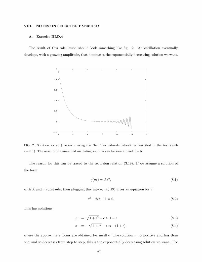
A. Exercise III.D.4

The result of this calculation should look something like fig. 2. An oscillation eventually

develops, with a growing amplitude, that dominates the exponentially decreasing solution we want.

-0.2

0

0.2

0.4

0.6

0.8

1

0 2 4 6 8 10 12

FIG. 2: Solution for y(x) versus x using the “bad” second-order algorithm described in the text (with

ε = 0.1). The onset of the unwanted oscillating solution can be seen around x = 5.

The reason for this can be traced to the recursion relation (3.19). If we assume a solution of

the form

y(nε) = Azn, (8.1)

with A and z constants, then plugging this into eq. (3.19) gives an equation for z:

z2 + 2εz − 1 = 0. (8.2)

This has solutions

z+ =√

1 + ε2 − ε ≈ 1− ε (8.3)

z− = −√

1 + ε2 − ε ≈ −(1 + ε), (8.4)

where the approximate forms are obtained for small ε. The solution z+ is positive and less than

one, and so decreases from step to step; this is the exponentially decreasing solution we want. The

27

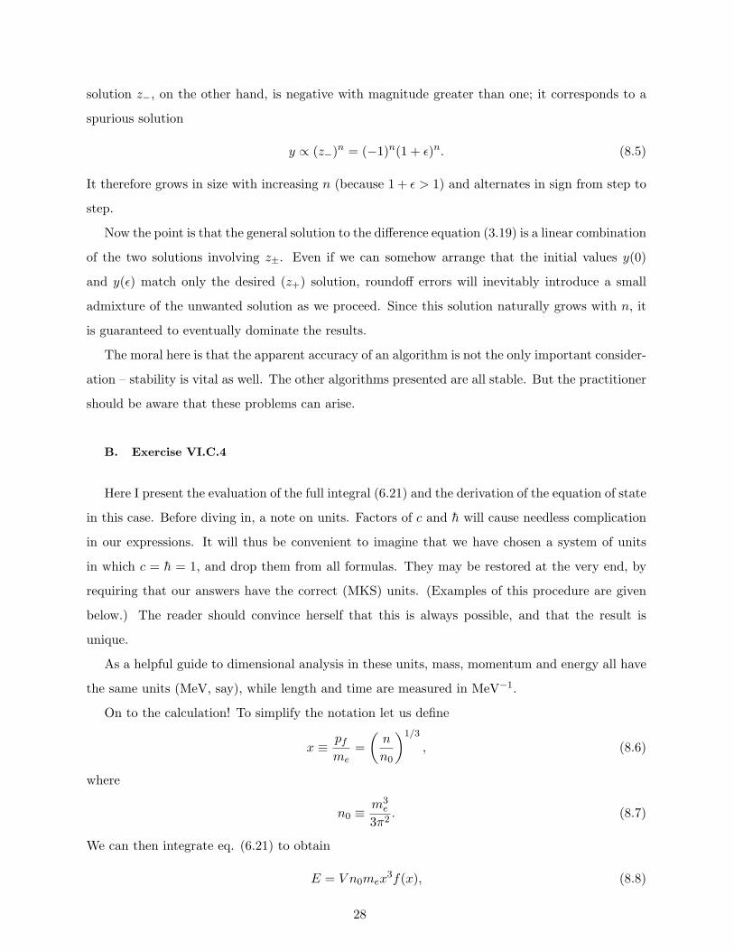
solution z−, on the other hand, is negative with magnitude greater than one; it corresponds to a

spurious solution

y ∝ (z−)n = (−1)n(1 + ε)n. (8.5)

It therefore grows in size with increasing n (because 1 + ε > 1) and alternates in sign from step to

step.

Now the point is that the general solution to the difference equation (3.19) is a linear combination

of the two solutions involving z±. Even if we can somehow arrange that the initial values y(0)

and y(ε) match only the desired (z+) solution, roundoff errors will inevitably introduce a small

admixture of the unwanted solution as we proceed. Since this solution naturally grows with n, it

is guaranteed to eventually dominate the results.

The moral here is that the apparent accuracy of an algorithm is not the only important consider-

ation – stability is vital as well. The other algorithms presented are all stable. But the practitioner

should be aware that these problems can arise.

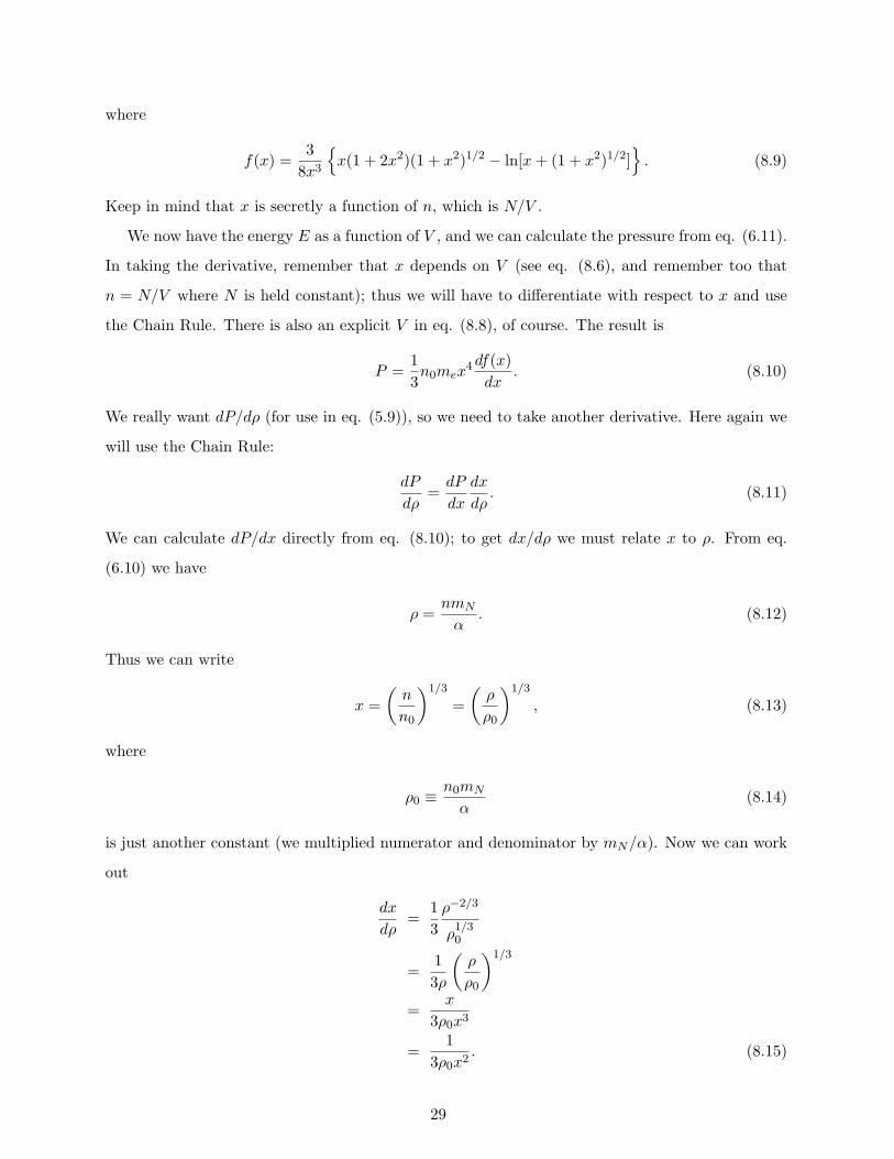
B. Exercise VI.C.4

Here I present the evaluation of the full integral (6.21) and the derivation of the equation of state

in this case. Before diving in, a note on units. Factors of c and h̄ will cause needless complication

in our expressions. It will thus be convenient to imagine that we have chosen a system of units

in which c = h̄ = 1, and drop them from all formulas. They may be restored at the very end, by

requiring that our answers have the correct (MKS) units. (Examples of this procedure are given

below.) The reader should convince herself that this is always possible, and that the result is

unique.

As a helpful guide to dimensional analysis in these units, mass, momentum and energy all have

the same units (MeV, say), while length and time are measured in MeV−1.

On to the calculation! To simplify the notation let us define

x ≡pfme

=(n

n0

)1/3

, (8.6)

where

n0 ≡m3e

3π2. (8.7)

We can then integrate eq. (6.21) to obtain

E = V n0mex3f(x), (8.8)

28

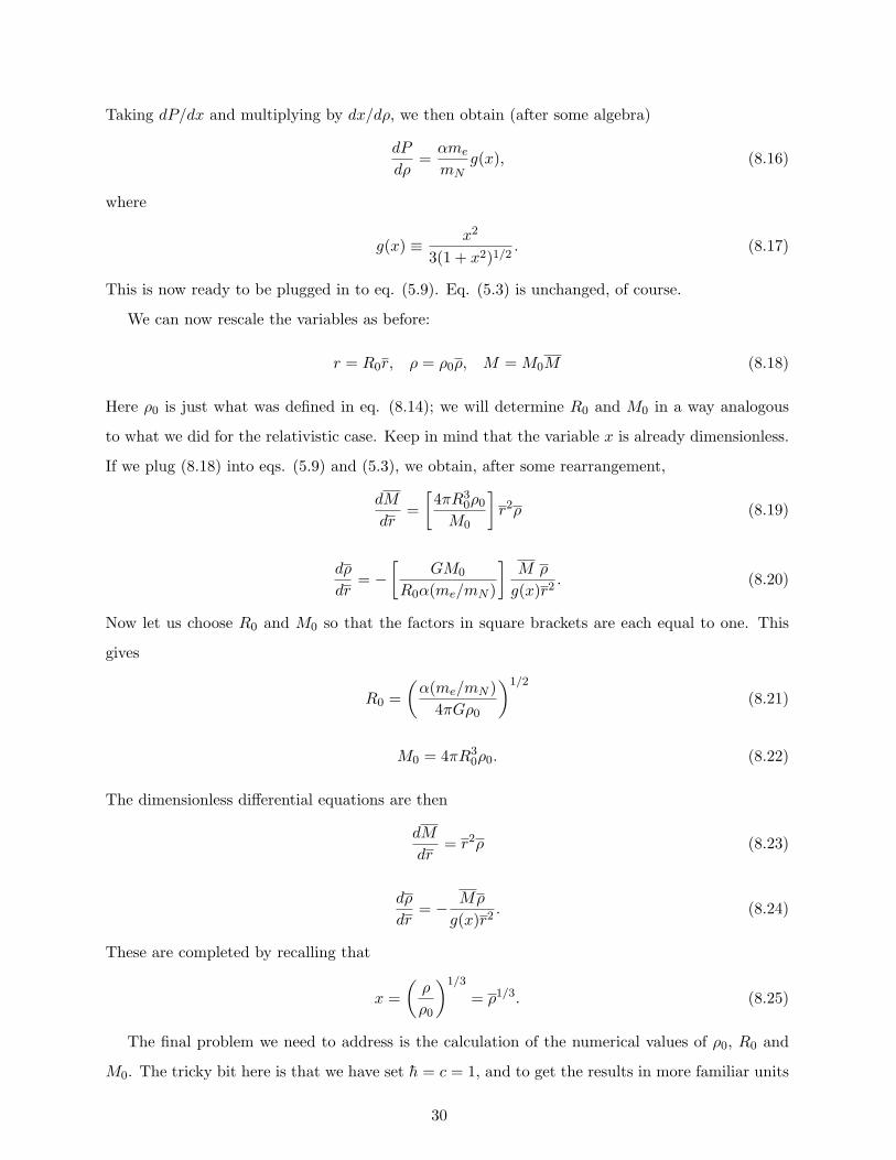
where

f(x) =3

8x3

{x(1 + 2x2)(1 + x2)1/2 − ln[x+ (1 + x2)1/2]

}. (8.9)

Keep in mind that x is secretly a function of n, which is N/V .

We now have the energy E as a function of V , and we can calculate the pressure from eq. (6.11).

In taking the derivative, remember that x depends on V (see eq. (8.6), and remember too that

n = N/V where N is held constant); thus we will have to differentiate with respect to x and use

the Chain Rule. There is also an explicit V in eq. (8.8), of course. The result is

P =13n0mex

4df(x)dx

. (8.10)

We really want dP/dρ (for use in eq. (5.9)), so we need to take another derivative. Here again we

will use the Chain Rule:

dP

dρ=dP

dx

dx

dρ. (8.11)

We can calculate dP/dx directly from eq. (8.10); to get dx/dρ we must relate x to ρ. From eq.

(6.10) we have

ρ =nmN

α. (8.12)

Thus we can write

x =(n

n0

)1/3

=(ρ

ρ0

)1/3

, (8.13)

where

ρ0 ≡n0mN

α(8.14)

is just another constant (we multiplied numerator and denominator by mN/α). Now we can work

out

dx

dρ=

13ρ−2/3

ρ1/30

=13ρ

(ρ

ρ0

)1/3

=x

3ρ0x3

=1

3ρ0x2. (8.15)

29

Taking dP/dx and multiplying by dx/dρ, we then obtain (after some algebra)

dP

dρ=αme

mNg(x), (8.16)

where

g(x) ≡ x2

3(1 + x2)1/2. (8.17)

This is now ready to be plugged in to eq. (5.9). Eq. (5.3) is unchanged, of course.

We can now rescale the variables as before:

r = R0r, ρ = ρ0ρ, M = M0M (8.18)

Here ρ0 is just what was defined in eq. (8.14); we will determine R0 and M0 in a way analogous

to what we did for the relativistic case. Keep in mind that the variable x is already dimensionless.

If we plug (8.18) into eqs. (5.9) and (5.3), we obtain, after some rearrangement,

dM

dr=[

4πR30ρ0

M0

]r2ρ (8.19)

dρ

dr= −

[GM0

R0α(me/mN )

]M ρ

g(x)r2. (8.20)

Now let us choose R0 and M0 so that the factors in square brackets are each equal to one. This

gives

R0 =(α(me/mN )

4πGρ0

)1/2

(8.21)

M0 = 4πR30ρ0. (8.22)

The dimensionless differential equations are then

dM

dr= r2ρ (8.23)

dρ

dr= − Mρ

g(x)r2. (8.24)

These are completed by recalling that

x =(ρ

ρ0

)1/3

= ρ1/3. (8.25)

The final problem we need to address is the calculation of the numerical values of ρ0, R0 and

M0. The tricky bit here is that we have set h̄ = c = 1, and to get the results in more familiar units

30

(like m and kg) we need to put these factors back. It turns out that there is always one unique way

to put factors of h̄ and c into any formula so that the units work correctly. So the basic problem

is to use dimensional analysis to figure out where they must go. For example, consider

ρ0 =n0mN

α=m3e

3π2

mN

α. (8.26)

This is a density, so it must have units of kg/m3, but the right hand side has (MKS) units of

kg4. There is only one way to add factors of h̄ (which has dimensions energy times time) and c

(dimensions length over time) to the right hand side to make a density; I claim it is

ρ0 =n0mN

α=m3e

3π2

mN

α

c3

h̄3 . (8.27)

You should check this! (Remember that α has no units.) Now we can plug in all the constants to

get

ρ0 =9.8× 108

α

kgm3

. (8.28)

Similarly, we can figure out where the factors of h̄ and c go in eqs. (8.21) and (8.22) by requiring

that these have units of length (m) and mass (kg) respectively. The results are

R0 =(α(me/mN )

4πGρ0

)1/2

c (8.29)

M0 = 4πR30ρ0. (8.30)

I leave it to you to work out their numerical values.

[1] J.B. Hartle, Gravity: An Introduction to Einstein’s General Relativity (Addison Wesley, 2003).

[2] S.M. Carroll, Spacetime and Geometry: An Introduction to General Relativity (Benjamin Cummings,

2003).

[3] S.E. Koonin, Computational Physics (Benjamin/Cummings, 1985).

[4] T. Pang, An Introduction to Computational Physics (Cambridge University Press, 2006).

[5] L.D. Fosdick, E.R. Jessup, C.J.C. Schauble, and G. Domik, Introduction to High-Performance Scientific

Computing (MIT Press, 1996).

[6] See, for example, E. Chaisson and S. McMillan, Astronomy, A Beginner’s Guide to the Universe, 5th

ed. (Prentice Hall, 2007); R.A. Freedman and W.J. Kauffmann, Universe, 8th ed. (W.H. Freeman,

2008).

[7] L.D. Landau, “On the Theory of Stars,” in Collected Papers of L.D. Landau, D. ter Haar, ed. (Gordon

and Breach, 1965).

31

[8] S. Chandrasekhar, Ap. J. 74 81 (1931). Chandrasekhar won the 1983 Nobel Prize for his work on stellar

structure. His Nobel lecture, available at http://nobelprize.org/, gives a nice overview of this work.

[9] See, for example, S. Weinberg, Gravitation and Cosmology (Wliey, 1972).

[10] J.R. Oppenheimer and G.M. Volkov, Phys. Rev. 55, 374 (1939).

[11] R.R. Silbar and S. Reddy, Am. J. Phys. 72, 892 (2004); Erratum ibid. 73, 296 (2005).

[12] In practice things are not so simple. On a computer, where real numbers are represented in a discrete

fashion, problems will arise if ε is made too small. The precise nature of the problem will depend on

the details of our scheme, and a detailed discussion of these issues would take us too far afield. For the

moment just keep in mind that ε cannot be made too small in practice.

[13] This is called “roundoff error” because it can be thought of as arising from rounding the results of cal-

culations from their true mathematical values to values that are actually represented on the computer.

[14] This is just the same as determining the ground state configuration of a multi-electron atom, by filling

orbitals of increasing energy with electrons, two per state. The only difference is that here the “orbitals”

(single-particle wavefunctions) are especially simple

[15] The appearance of Newton’s constant G along with c in the third term is a sign that this is a general

relativistic correction.

32

Glossary

beta decay Weak interaction decay of a neutron to a proton, electron and

an electron anti-neutrino. For free neutrons the half life is

about 14 minutes.

black hole End state of a very massive star; a spacetime configuration

from which neither material particles or light can escape.

boson Particle with integer spin; not required to obey the Exclusion

Principle. Examples include the photon.

Chandrasekhar mass Maximum theoretical mass of a white dwarf, about 1.4 solar

masses.

equation of state Relation between pressure and density, characterizing the

macroscopic properties of matter.

Euler method Simple method of integrating an ODE based on approximating

differentials by differences. Not recommended for practical use

due to poor accuracy.

Exclusion Principle Statement that no two identical fermions may occupy the same

quantum state.

Fermi gas Collection of non-interacting fermions.

Fermi momentum Highest magnitude of momentum that occurs in the Fermi sea.

Fermi sea The ground state configuration of a set of fermions.

fermion Particles that have half-integer spin, and also obey the Ex-

clusion Principle. Examples include electrons, protons and

neutrons.

general relativity Einstein’s theory of gravity, in which spacetime curvature gives

rise to gravitational effects.

neutron star Possible end state of a star after nuclear reactions have ceased,

in which the star is supported by nuclear repulsion between

neutrons

33

nuclear fusion Reaction in which two nuclei fuse together, perhaps releasing

other particles and either releasing or absorbing energy.

nucleon Proton or neutron.

ordinary differential equation An equation for a function of one independent variable, involv-

ing derivatives of that function.

polytrope A simple power law equation of state, of the form P = Kργ .

round-off error Error in floating-point computations on a computer introduced

due to the discrete representation of real numbers.

Runge-Kutta A numerical integration algorithm.

Skyrme model Phenomenological model of nuclear interactions in which nu-

clear forces are contact forces (zero range).

strong nuclear interaction A fundamental interaction in nature. An elementary interac-

tion between quarks, it is manifested as a residual interaction

between nucleons.

symmetric nuclear matter Nuclear matter with equal numbers of protons and neutrons.

symmetry energy The part of the nuclear matter energy that is sensitive to the

asymmetry between protons and neutrons.

TOV equation Tolman-Oppenheimer-Volkov equation. The basic equation

expressing the requirement of hydrodynamics equilibrium for

a spherical star, including lowest-order relativistic corrections.

white dwarf Possible end state of a star after nuclear reactions have ceased,

in which the star is supported by electron degeneracy pressure

34