The structure of simple New Economic Geography models (or ...frobertnicoud.weebly.com/uploads/9/5/6/1/9561580/joeg_2005.pdf · Keywords: New Economic Geography, natural state space,

Journal of Economic Geography 5 (2005) pp. 201–234Advance Access originally published online on 4 November 2004 doi:10.1093/jnlecg/lbh037

The structure of simple ‘New EconomicGeography’ models (or, On identical twins)Frederic Robert-Nicoud*

AbstractThispapershowsthat themathematicalstructureof themostwidelyusedNewEconomic Geography models is identical, irrespective of the underlyingagglomeration mechanism assumed (factor migration, input-outputlinkages, endogenous capital accumulation). This enables us to provide analy-tical proofs to four important and related results in the field. First, standardmodels display at most two interior steady states beyond the symmetric one.Second,wheninterior,asymmetricsteady-statesexisttheyareunstable.Third,location displays hysteresis. Finally, with forward looking agents a shock toexpectations might trigger an equilibrium switch. This paper also stresses theempirical implications of the most important results derived in this study.

Keywords: New Economic Geography, natural state space, number of steady-states, stability,

hysteresis, expectations

JEL classification: C62, D58, F12, R12

Date submitted: 2 March 2004 Date accepted: 9 April 2004

1. Introduction

The notion of space and its relation to economic activities has been studied as early as in

the nineteenth century with the work of von Th€uunen in 1826 and others. More recent work

by Krugman (1991a,b) and others revived the mainstream economists’ interest in the

topic. This work relies heavily on the monopolistic competition framework put forth by

Dixit and Stigltz (1977) (DS hereafter). This new avatar of spatial economics became

known as the ‘New economic geography’, or NEG for short. Three recent monographs

assess the progress made in this new paradigm since the seminal work of Paul Krugman.

These, together with the recently born Journal of Economic Geography, attest the vividinterest for this topic.1 More generally, the book by Fujita and Thisse (2002) is probably

the most exhaustive source on the topic for it unifies the spatial economics field from

von Th€uunen to Krugman.

* Departement d’Economie Politique, University of Geneva, Bd. Du Pont d’Arve 40, 1211 Geneva 4,Switzerland; and CEPR.email <[email protected]>

1 Fujita et al. (1999) deals with several positive issues; Brakman, Garretsen, and van Marrewijk (2001) is anon-technical textbook; and Baldwin, Forslid, Martin, Ottaviano, and Robert-Nicoud (2003a) apply NEGmodels to various policy issues. Peter Neary (2001), who critically evaluates the progress made in the field inhis JEL paper, might add: ‘what next?The T-shirt?The Movie?’ A good guess is probably a book devoted toempirical evidence; see Overmanet al. (2003) andHead and Mayer (2004) for two recent surveys ofempiricalwork in Geography and Trade.

Journal of Economic Geography, Vol. 5, No. 2, # Oxford University Press 2005; all rights reserved.

The main insight of the NEG comes from its formalization of agglomerationmechanisms based on endogenous market size.2 Various trade models predict that

sectors characterized by increasing returns to scale, imperfect competition, and

transportation costs will be disproportionately active in locations with good market

access (Krugman, 1980). In a simple two-country model, this ‘home market effect’

implies that the country with the larger demand for the good produced by such sector

will end up exporting that good (this result sharply contrasts with the predictions of the

Ricardian and Heckser-Ohlin-Viner models of trade). NEG models add cumulative

causation to this effect: hosting a larger share of increasing returns activities increaseslocal demand and profitability. If there is factor mobility of sorts, then more of these

factors will in turn locate themselves in the already large market, and the cycle repeats

under certain conditions. Endogenous agglomeration results from this mechanism.

Therefore, initially symmetric regions might end up hosting very different sectors as

increasing returns activities have a tendency to locate in few places (Fujita and Thisse,

2002). As for the transmission mechanism whereby agglomeration occurs, the NEG

exploits in a spatial setting the kind of circularity causality recurrent in models of

monopolistic competition (Matsuyama, 1995).3

The beauty of the neoclassical trade theory stems for a good part on its ability to provide

systematic predictions relying on few assumptions and robust to the choice of functional

form (e.g., the two-factor, two-sector model of Jones, 1965). By contrast, to this day there

is no unified NEG theory and there might not be any for years to come. Instead, various

authors have provided a gallery of illuminating examples based on specific functional

forms. Until recently, all contributions were exclusively based on the DS model of

monopolistic competition.4 Moreover, the cumulative causation makes these models

cumbersome to analyse. As a result, they were initially explored numerically (seeMaffezzoli and Trionfetti, 2002, for recent methodological improvements in numerical

simulations of Krugman’s model). The problem with this is that, though these numerical

examples are insightful, we cannot be sure that they provide an exhaustive description of

the model’s characteristics (Baldwin et al., 2003a,b).

Fortunately, many results became available by analytical means over time. The first

contribution of this paper is in the continuation of this task. To evaluate this first

contribution, it is useful to have an idea of the structure of equilibria of DS-based

NEG models. In such models, locations are typically ex ante identical (identicalpreferences, same technology, and same endowment of immobile factors). As a result,

there always exists a symmetric equilibrium where locations have equal shares of mobile

factors and economic activities (in particular the increasing returns sector). However, this

equilibrium may or may not be stable. There may also be an equilibrium in which all

2 Its emphasis on market size makes this literature at the crossroad of the ‘new international trade theory’(Helpman and Krugman, 1985) and spatial economics.

3 See also Matsuyama and Takahasi (1998) on this issue in a different spatial model. These authors conductwelfare analysis and show how the coordination failures between migration decisions of individuals andentry decisions of firms typically result in inefficiencies at the long run equilibrium location.

4 Ottaviano et al. (2002) propose an alternative framework based on quadratic subutilities rather than CES.This model is much simpler to handle than the models based on DS monopolistic competition and displayspro-competitive effects that are absent in the DS framework. However, its dynamic properties are less richthan in the latter framework. See Ottaviano and Thisse (2004) and Baldwin et al. (2003a) for detailedanalysis of the differences and similarities between these two frameworks.

202 � Robert-Nicoud

increasing returns production is clustered in a single region. The first analytical result in theNEG literature was to derive the set of parameters (summarized by the ‘sustain point’ in the

NEG lexicon) under which this agglomeration equilibrium exists (Krugman, 1991b).

The second analytical result is due to Puga (1999). Among other things, Diego Puga’s

paper shows that it is possible to linearize the model around the symmetric equilibrium and

to derive a closed-form solution for the set of parameters under which the equilibrium is

(locally) stable, that is, for the so-called ‘break point’. Finally, Baldwin (2001) showed that

the informal methods developed in Krugman (1991b) and subsequent papers, as well as

the ad hoc law of motions, can be rationalized. In particular, he shows that the conditionsunder which the equilibria are locally stable are also valid to asses their global stability.

However, two results remain unproven. First, the literature studies only one interior

equilibrium (the symmetric one) even though there exist other interior equilibria for some

parameter values. Hence, the focus of analysis on a very particular interior equilibrium

and the full agglomeration equilibria of the current literature would be incomplete if there

existed other stable equilibria. In this paper I prove that there are at most three interior

equilibria and that, whenever they exist, the interior asymmetric equilibria are unstable.5

This establishes that the disdain of the literature for the latter is justified.Second, several recent important contributions of the literature rely on the possibility

of location hysteresis. This is notably the case for some results in the burgeoning literature

on tax competition in a NEG framework. This literature questions the received

(neoclassical) wisdom in spectacular ways.6 Location hysteresis implies that there are

agglomeration rents that can be taxed without inducing the mobile factor (the tax base)

to move out. To understand the nature of these rents, it is important to realize that

agglomeration generates inertia: to put it colloquially, people and firms are there

because other people and firms are there, too. So people are willing to move out of theagglomeration only if a large chunk of other people are willing to do so as well. Therefore,

a large shift in the policy environment is needed to give incentives to a large number of

people to move and thus shake inertia (see Baldwin et al., 2003a, for details).

It turns out that these agglomeration rents are bell-shaped in transportation costs,

which in turn implies that there might be a ‘race to the top’ (Baldwin and Krugman, 2004)

in the taxation of the mobile factor when transportation costs decline (a short-cut for

economic integration or ‘globalization’). Most of the models to which the analysis of the

current paper applies (listed in Table 1) have a range of parameters where both thesymmetric and the agglomeration equilibria are stable. The existence of this range

implies that self-fulfilling expectations are a possibility when workers are forward

looking. In other words, shocks to expectations can trigger a jump between the

symmetric equilibrium and the agglomeration outcome (Baldwin, 2001, Baldwin et al.,

2003a). In any case, the issue of the existence of this range pertains to ranking the break

and sustain points.7 In this paper, I prove that the set of parameters such that both kind of

equilibria are simultaneously stable is non empty. Following an early manuscript version

of this paper, this important result has been incorporated in Neary (2001) and Fujitaand Thisse (2002) (here I generalize it to all models of Table 1).

5 This last result is quite specific to the models studied in the current paper. I will get back to this in Section 4.

6 See e.g., Andersson and Forslid (2003), Baldwin et al. (2003a), Kind et al. (2000), and Ludema and Wooton(2000). On the political economics of regional subsidies, see Robert-Nicoud and Sbergami (2004).

7 This is by no means a trivial task because the expression for the sustain point is a non-linear, implicit equation.

The structure of simple NEG models � 203

The proof of the first result works by showing that the most common variants of the

core model in this literature are isomorphic at equilibrium in a certain, economicallymeaningful, state space. For this reason, I will dub it as the ‘natural’ state space. This

allows us to prove results in the most tractable version and to apply those in the most

intractable variants. In other words, the method of proof also tells us something deep

about NEG models: even though they are a collection of illuminating examples (to

paraphrase Jacques Thisse), these examples convey some degree of generality. Before

turning to the analysis proper, let me digress a bit on this last point.

1.1. On the generality of the properties of the Krugman model

The common point between most NEG models is the combination of Dixit-Stiglitz

monopolistic competition with iceberg transportation costs (Samuelson, 1952) andsome sort of factor mobility.8 Turn to Table 1, which classifies some contributions in

this paradigm along two dimensions. Start with the vertical differentiation. Models in the

left column add endogenous market size to the original trade model due to Krugman

(1980). Papers that belong to the second column do likewise using an alternative

functional form put forth by Flam and Helpman (1987). The horizontal classification

discriminates among models according to the mechanism whereby the market size is

endogenous. The seminal paper by Krugman (1991b) combines the former functional

form with migration of the factor used intensively in the increasing returns sector.The resulting core-periphery (or CP) model is extraordinarily difficult to work with,

which partly explains why it took so many steps to get a more or less comprehensive

8 More specifically, preferences take an upper-tier Cobb-Douglas form over an index of a homogeneous goodand the increasing returns good and a lower-tier CES form among the increasing returns’ varieties. Bycontrast, in Ottaviano et al. (2002) preferences are quasi-linear for the upper-tier and quadratic for the lowertier. Pfl€uuger (2003) conveys some cross-breading: he assumes quasi-linear upper-tier preferences (likeOttaviano et al., 2002) and CES sub-utility (like Krugman, 1991b). Interestingly, asymmetric interiorequilibria are stable when they exist in his setting.

Table 1. Three classes and 13 years of economic geography models

Underlying model

Krugman (1980) Flam and Helpman (1987)

Factor migration CP (core-periphery) FE (Footloose Entrepeneur)

Krugman (1991b) Forslid and Ottaviano (2003)

Input-output linkages

(a.k.a. vertical linkages)

CPVL (core-periphery,

vertical linkages)

FCVL (footloose capital,

vertical linkages)

Krugman and Venables Robert-Nicoud (2002)

(1995) FEVL (Footloose entrepreneur,

vertical linkages)

Ottaviano (2002) and

Ottaviano and Robert-Nicoud

(2003)

Factor accumulation CC (constructed capital)

Baldwin (1999)


list of its properties. Its closest cousin is the ‘footloose entrepreneur’ (or FE) model due toForslid and Ottaviano (2003) (the terminology is borrowed from Baldwin et al., 2003a).

This model is very similar to Paul Krugman’s original version but is much easier to

manipulate because its use of the Flam-Helpman functional form allows for closed-

form solutions unachievable in the Krugman framework.

In Krugman and Venables (1995), which simplified and popularized the mechanism put

forth by Venables (1994, 1996), firms belonging to the increasing returns sector buy each

others’ output as intermediate inputs (hence the name vertical linkages). Workers, though

immobile across regions, move freely across sectors. This way, the market size relevant tothe increasing sector is endogenous. Again, analytical results in this framework are

rare and very difficult to obtain. For this reason, Ottaviano (2002) and Robert-

Nicoud (2002) developed alternative vertical linkage models, each using the Flam-

Helpman specification.9 The latter model combines perfect (physical) capital mobility

with vertical linkages. See Appendix 2 for a sketch of this model.

Finally, Baldwin (1999) proposes a model in which endogenous (human) capital

accumulation makes the market size endogenous. Like all analyst-friendly models,

Richard Baldwin’s uses the Flam-Helpman functional form (see also Appendix 2).It is worth mentioning that Puga (1999) combines factor migration and vertical linkages

using Krugman’s (1980) functional form whereas Faini (1984) combines vertical linkages

and endogenous factor accumulation, albeit in a different setting.

With the exception of Faini (1984), all papers mentioned above and enlisted in Table 1 are

isomorphic in a certain, economically meaningful, state space. An analogy with identical

twins is helpful to understand the depth of the similarities among these apparently

different models. Like identical twins, they share the same genome (or intrinsic

properties). But even identical twins look a bit different and have different characters.Also, they are different individuals who might dress up differently.

This is a remarkable result in itself. Indeed, it shows that the stability properties of these

models are identical despite their using of different functional forms and agglomeration

mechanisms. This falls short of having a general theory, but nevertheless suggests that the

main results derived by Krugman (1991b) and others have some degree of generality and

should be pervasive to changes of functional forms.10 For lack of space, I will show that

this is the case for only three of the models in Table 1: the CP model by Krugman (1991b),

the FE model due to Forslid and Ottaviano (2003), and, in Appendix 2, the FCVL modeldue to Robert-Nicoud (2002). In a related paper, Ottaviano and Robert-Nicoud (2003)

convey the same message for better known models based on vertical linkages.11

Nevertheless, I will mention in passing and in the conclusion how this method applies

to such VL models as well as to Baldwin’s (1999) growth model.

The remainder of the paper is organized as follows. The section immediately after this

introduces the notation, spells out the canonical CP model, and derives the equilibrium

conditions in the new state space. Section 3 then does the same for the FE model and

shows that the CP and FE models are isomorphic. Section 4 formally characterizes theset of steady-states and derives their stability properties: In particular, Proposition 3

9 See also Baldwin et al. (2003a, ch.8) and Ottaviano and Robert-Nicoud (2003).

10 See also footnote 4 on this.

11 Ottaviano and Robert-Nicoud (2003) also convey the welfare analysis of VL models borrowing from themethodology developed by Charlot et al. (2003) for the CP model.


establishes that there are at most three interior equilibria. Proposition 5 establishes thatthese models open the possibility for shocks to expectations to generate a switch from

one equilibrium to another. Finally, Section 5 concludes in briefly sketching how other

standard NEG models also fit into the natural state space and equations, and hence how

theproofdevelopedinthispapereasilyextendstoVLandBaldwin’s(1999)models.Thisfinal

section also addresses the empirical implications of the main results derived in the paper.

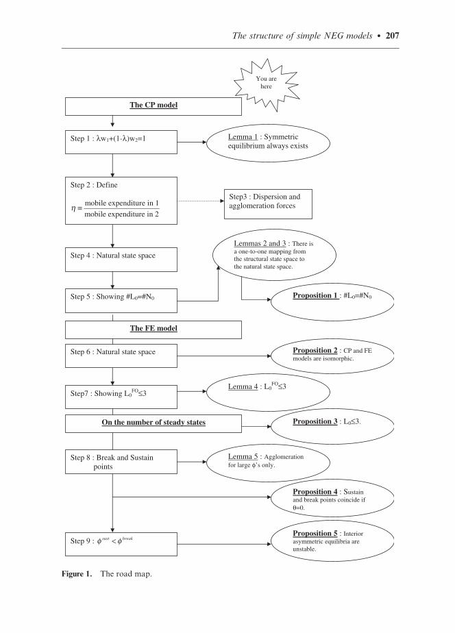
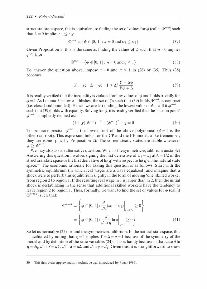
Since the paper and the method of proof are slightly long, it might be useful to have

a road map to which the reader can refer when she feels lost. In Figure 1 I have sketched

the various steps that are necessary to derive the various Lemmas and Propositions ofthe paper.

2. The ‘natural’ state space for migration-based models

This section introduces the notation and establishes the state space in which the

migration-based CP and FE models are isomorphic. This is the first necessary

intermediate step on our way to establish the main results of Section 4.

2.1. The common structure

Common to virtually all NEG models are two regions (indexed by j¼ 1, 2) and two sec-

tors. The background sector A (agriculture) produces a homogenous good under constant

returns to scale (or CRS) in a perfectly competitive environment using unskilled workers

(whose wages are denoted by wU) only; its output is freely traded; consumers spend a share

1�m of their expenditure on A. The ‘manufacturing’ sector M produces a differentiated

product under increasing returns to scale (or IRS) in a monopolistically competitive

environment a-la Dixit and Stiglitz (1977) using skilled workers only (whose wages

are denoted by w). Denote the elasticity of substitution between any two varieties bys>1 Shipping this good into the other region involves ‘iceberg’ transportation costs: T>1

units need to be shipped so that 1 units arrives at destination; the rest, T� 1, melts in

transit. Consumers spend a share of their expenditure 0<m< 1 on the composite M.

Specifically, tastes are described by the following function:

U ¼ C1�mA C

mM , CM ¼

Znw

i¼0

cðiÞ1�1=sdi

0@

1A

11�1=s

, 05m515s ð1Þ

where CA is the consumption of good A and CM is the (index) consumption of M. This

good comes in nw different varieties indexed by i (nw will be determined at equilibrium);c(i) is the quantity consumed of variety i. Furthermore, in models based on factor

migration under consideration here, each region is endowed with LU/2 unskilled

workers. Both regions also share L skilled workers, with l (respectively 1� l) of them

living in region 1 (resp. 2); l is the endogenous variable of interest.

In short, we have:

m—the expenditure share on M goods

nw—the mass (or the number) of available M-varieties

s—the elasticity of substitution among the nw varieties

LU/2—the mass of unskilled worker in region j 2 {1, 2}

lL—the mass of skilled workers in region 1.


Step 1 : λw1+(1-λ)w2=1

Step 2 : Define

mobile expenditure in 1

mobile expenditure in 2η ≡

Step 4 : Natural state space

Step3 : Dispersion and agglomeration forces

Step 5 : Showing #L0=#N0 Proposition 1 : #L0=#N0

Lemmas 2 and 3 : There isa one-to-one mapping from the structural state space tothe natural state space.

Lemma 1 : Symmetricequilibrium always exists

The FE model

Step 6 : Natural state space

Step 9 : sust breakφ φ<

Proposition 2 : CP and FEmodels are isomorphic.

Step 8 : Break and Sustain points

Step7 : Showing L0FO≤3

Lemma 4 : L0FO≤3

Lemma 5 : Agglomeration for large φ’s only.

Proposition 3 : L0≤3.On the number of steady states

Proposition 4 : Sustainand break points coincide ifθ=0.

Proposition 5 : Interiorasymmetric equilibria are unstable.

The CP model

You are here

Figure 1. The road map.


2.2. The CP model

In Krugman’s (1991b) CP model, each factor is specific to a different sector: the

background (resp. manufacturing) sector uses unskilled (skilled) workers only. In

particular, the cost function of the typical M-firm takes the following form:

CðxðiÞÞ ¼ w½F þ rxðiÞ� ð2Þ

where x(i) is the firm output, F is the fixed labour requirement, r is the variable labour

requirement, and w is the (skilled) labour wage; for clarifying purposes, w will be indexed

by a subscript 1 or 2 so as to distinguish between regions when necessary.

2.3. Normalizations

Following Fujita et al. (1999), let us make the following normalizations.12 First, we take A

as the numeraire. Second, we can choose units in which manufacturing output and labour

are measured. As stressed by Puga (1999), these involve choosing a value for r and F,

respectively:

The variable labour requirement in (2): r ¼ 1 � 1=s

The fixed labour requirement in (2): F ¼ m=s

The fact that we choose a value for both the marginal labour requirement r and the fixed

labour requirement F might worry some readers. These normalizations are perfectly valid,

though, because the cost function (2) is homothetic. This assumption, together with free-entry, ensures that total input requirement is independent of marginal input requirement;

the variable that adjusts is the total number of firms.

By the same token, we can choose units in which output in sector A is measured:

Sector A labour-output requirement is 1

The latter normalization implies wU¼ 1 in each region, whereas the normalization on

the variable labour requirement in the M sector simplifies the equilibrium pricing

expressions. The final choices of units we make concern the exogenous supply of

primary factors. Because these are continuous variables, we can measure them in

anyway we want. Following Krugman (1991a,b) we choose L and LU so that nominal

wages are equalized at the symmetric equilibrium. Assuming that l¼ 1/2 implies

w¼wU¼ 1 requires:

Labour endowments: LU=L ¼ ð1 � mÞ=m

It turns out that this normalization also implies that nominal wages are equalized

throughout in the agglomerated equilibria, a priori when l¼ 0, 1. Going slightly

beyond the model, one might justify this assumption by saying that, deep down, thereshould be no persistent difference in the rewards workers might earn, regardless of the

sector in which they work.

12 Some of these normalizations might look a bit weird to the reader unfamiliar with the NEG (see Neary,2001). However, since we are assuming a continuum of varieties we are given an extra degree of freedom thatcan be absorbed in an extra normalization. In other words, the normalizations below entail no loss ofgenerality. See Baldwin et al. (2003a, box 2.2) on this point.


2.4. Instantaneous equilibrium in the CP model

With all these assumptions at hand, we can solve the model treating l as a parameter to

get the so-called ‘instantaneous’ (or ‘short run’) equilibrium. Such an equilibrium is

defined for a given value of l as a situation where all markets clear and trade is

balanced. Let us start with the demand side. Maximization of (1) under the constraint

that expenditure must not exceed disposable income Y yields:

CA;j ¼ ð1 � mÞYj; cjðiÞ ¼pjðiÞ�s

Gj

mYj , Gj �Znw

i¼0

pjðiÞ1�sdi

0@

1A

11�s

ð3Þ

where pj(i) is the consumer price of variety i in region j and Gj is the true manufacturingprice index. By (2) and our normalization for r, it is readily established that operating

profits are equal to:

pjðiÞ ¼pjðiÞcjðiÞ

sþ T

pkðiÞckðiÞs

, k 6¼ j ð4Þ

Note that the iceberg formulation for transportation costs implies that the firm does

actually ship Tck(i) units of i so that c(i) units arrive in the region k 6¼ j.

We now turn to the supply side. First, profit maximization of (2)–(4) gives the followingoptimal consumer pricing policy for the typical variety i produced in region j:

pjðiÞ ¼rwj

1 � 1=s¼ wj ; pkðiÞ ¼

rwj

1 � 1=sT ¼ Twj , k 6¼ j ð5Þ

where the second equality in both expressions above stems from our choice of units and

normalizations. Note that (5) implies markup pricing (that is, each manufacturer is

a monopolist in his own variety). This markup is constant (a function of tasteparameters only) and transportation costs are fully passed onto consumers (f.o.b.

pricing is typical of DS monopolistic competition).

Plugging (5) into (4), we obtain:

pjðiÞ ¼ pjðiÞ1�s mYj

sG1�sj

þ ðpjðiÞTÞ1�s mYk

sG1�sk

, k 6¼ j ð6Þ

A region’s total disposable income is defined as the labour income of its various

inhabitants. With a proportion l of skilled labour living in region 1, this yields

(remember the normalizations):

Y1 ¼ 1 � m

2þ lm, Y2 ¼ 1 � m

2þ ð1 � lÞm ð7Þ

Next, we assume that there is free entry and exit in the M sector. As a result, operating

profits must be equal to fixed costs at equilibrium for any active firm. Dropping the variety

index for now, this reads:

pj � xj pj � rwj

� ¼ wjF , xj ¼ x � Fðs � 1Þ

r¼ m ð8Þ

that is, the free-entry condition pins down the equilibrium firm size, given the pricing policy

(5). Note that this firm size is a function of parameters only (in particular, it is invariant

in wages). Also, the last equality in the expression above stems from the normalizations.


Third, we invoke the full employment condition of skilled labour to pin down theequilibrium number (mass) of available varieties.13 Labour supply is exogenously

given by L¼m. Labour demand is equal to:

nwðF þ rxÞ ¼ nw m

sþ rm

�¼ nwm ð9Þ

where I have successively made use of (8) and of the normalizations. As a result, full

employment of labour implies:

nw ¼ 1 ð10Þ

This completes the analysis of the ‘instantaneous’ equilibrium of the model. However, it is

impossible to get a closed-form solution for most endogenous variables of this model.

Instead, the short-run equilibrium is typically depicted by the following system ofequation that summarizes the results derived thus far (this system is identical to Fujita

et al., 1999, p.65):

Y1 ¼ mlw1 þ1 � m

2, Y2 ¼ mð1 � lÞw2 þ

1 � m

2

G1�s1 ¼ lw1�s

1 þ ð1 � lÞðTw2Þ1�s, G1�s2 ¼ lðTw1Þ1�s þ ð1 � lÞw1�s

2

ws1 ¼ Y1

G1�s1

þ T1�s Y2

G1�s2

, ws2 ¼ T1�s Y1

G1�s1

þ Y2

G1�s2

ð11Þ

The first line is a simple restatement of (7): income in region j, Yj, is defined as the sum of

skilled workers’ income (whose wage is wj) and unskilled workers’; income (whose wage isunity by choice of numeraire). To get the expression for the price indices in the second line,

plug (5) and (10) into the definition of Gj in (3). Finally, the expressions in the third line

combine (6) and (8). These are the free-entry-and-exit conditions (also called the ‘wage

equations’ in the jargon): firms in region j break even if they pay the wage wj.

2.5. Long run equilibrium in the CP model

In any instantaneous equilibrium, the expressions in (11) must hold simultaneously. A

long run equilibrium (or steady state) is defined as an instantaneous equilibrium in which,

in addition, the mobile factor has no incentive to migrate. Define the real (skilled labor)

wage in region j as vj, viz:

vj � wjG�mj ð12Þ

Hence, the system in (11) can be viewed as providing an implicit solution for v1�v2 asa function of l (and the parameters); accordingly, we write (11) as:

Fðv1 � v2, lÞ ¼ 0 ð13Þ

for short. Skilled labor is assumed to move from one region to the other so as to eliminatecurrent differences in real wages according to the following ad hoc law of motion:

l�¼ glð1 � lÞðv1 � v2Þ ð14Þ

13 Since there are no economies of scope, we can identify each variety with one firm.


where g > 0 is a parameter. Clearly, this means that expectations are static.14 A long run(or steady-state) equilibrium is defined as a combination of endogenous variables (that

now include l) that solves (11) and such that (14) holds for l�¼ 0. Two kinds of interior

steady states might occur. First are the corner solutions l2{0, 1}, namely, all mobile

workers are agglomerated in one region. In the jargon, such steady states are referred to as

‘core-periphery’ outcomes.15 Second, there are the interior solutions whereby l2(0,1) and

v1¼v2. Given the symmetry of the model, l¼ 1/2 is always part of an interior steady state

(see Lemma 1 in the immediate sequel). This particular case is usually referred to as the

‘symmetric equilibrium’. There might also exist other interior equilibria. Typically, theseequilibria are disregarded in the literature.

The issue of interest for the remainder of the section is the characterization of the

number of interior solutions, i.e. the number of l’s such that v1¼v2. Call the set of these

l’s L0, with l0 being the typical element of L0. That is:

L0 � fl 2 ½0, 1� : Fð0, lÞ ¼ 0g ð15Þ

Using (11), it is straightforward to show that the symmetric equilibrium always exists

(whereby an even repartition of skilled labour between the two regions entails identical

real wages) and that, whenever there exists an equilibrium in which real wages are

equalized for an uneven repartition of skilled workers, then the opposite, symmetric

repartition must also be part of a long run equilibrium (this is obvious because it only

involves a re-labelling of the two regions). In mathematical symbols, we write these

properties as the following lemma.

Lemma 1: First, l¼ 1/2 2 L0 is always true. Also, l0 2 L0 if, and only if, 1� l0 2 L0

Proof: Immediate by virtue of the symmetry of the model. QED.

So far all this is very well known, and we cannot really go further than this. Hence, the next

task is to rewrite (11) in an alternative state space that will prove very useful to move on.

2.6. The CP model in the ‘natural’ state space

Step 1: First, I claim that aggregate (nominal) expenditure of mobile (that is, skilled)

workers is constant for all l:

lw1 þ ð1 � lÞw2 ¼ 1 ð16Þ

To see this, multiply both sides of the wage equations in (11) by w1�sj and the result follows

readily by using the income and price index equations. This property stems from the Cobb-

Douglas functional form of the upper-tier utility function.

Step 2: Next, define the parameter f as:

f � T1�s 2 ½0, 1Þ ð17Þ

14 Baldwin (2001), however, shows that this is merely an assumption of convenience. Indeed, allowing forrational expectations and sufficiently large quadratic migration costs does not alter the ‘break’ and ‘sustain’points definedbelownor the local stabilitypropertiesof the longrun equilibria. Yet, expectations can be self-fulfilling when migration costs are low enough, as in Matsuyama (1991) or Krugman (1991c).

15 For instance, take l¼ 1. In this case, all skilled workers and manufacturing firms are clustered in region 1—the core—and region 2 is void of manufacturing and, as such, is dubbed as the periphery.


or the ‘free-ness’ of trade (f is decreasing in T).16 We now move on by using the definitionof vj ( j¼ 1, 2) and plugging it into (11):

Y1 ¼ mlw1 þ1 � m

2, Y2 ¼ mð1 � lÞw2 þ

1 � m

2

G1�s1 ¼ lw1ðv1G

m

1 Þ�s þ fð1 � lÞw2ðv2G

m

2 Þ�s,

G1�s2 ¼ flw1ðv1G

m

1 Þ�s þ ð1 � lÞw2ðv2G

m

2 Þ�s

ðv1Gm

1 Þs ¼ Y1

G1�s1

þ fY2

G1�s2

, ðv2Gm

2 Þs ¼ f

Y1

G1�s1

þ Y2

G1�s2

ð18Þ

As is obvious from the expression above, operating profits are an increasing function of

income Yj. Also, the relative profitability of firms in each region depends, among other

things, on the relative income (expenditure) in each region. Moreover, this relative income

is endogenous in the model: it varies with the relative mobile expenditure. Indeed, when

skilled workers migrate they earn a different income from before and this, as much as

the fact that they migrate, changes market size. As we will see, this mobile expenditure

will play a crucial role in our task of rewriting the model in an alternative state

space. Accordingly, define the variable h as the ratio of the mobile factor’s expendi-ture in 1 to mobile expenditure in 2 (which is thus a measure of the relative market

size of region 1), namely:

h � lw1

ð1 � lÞw2ð19Þ

By virtue of (16), there is a one-to-one relationship between h on the one hand and lw1 and

(1� l)w2 on the other. As we shall see, h plays a fundamental role in the analysis.

Step 3: The third step involves the parameterization of some crucial forces

at work.

2.7. Agglomeration and dispersion forces

A digression on the agglomeration and dispersion forces is useful at this stage because it

boosts economic intuition. This discussion also makes sense of the definition of some

collections of parameters that are recurrent in the analysis to come.

2.7.1. Agglomeration force #1: Backward linkage

The discussion in the paragraph above points to the first agglomeration force present in

the model, known as the backward linkage (think about it as a demand linkage): when a

firm moves from, say 2, to region 1 the labour force increases in the destination region and

shrinks in the source region. As a result, the market size increases in the former and

decreases in the latter, thus, all things equal, making firms relatively more profitable in

region 1 (and higher profits translate into higher nominal wages given that firms break

even by assumption), so the cycle repeats. Of course, this agglomeration force is stronger

16 When f¼ 0 transportation costs are infinite and trade free-ness is nil. When f ¼ transportation costs areabsent (T¼ 1) and trade free-ness is total.


if skilled workers are numerous (L is large). To parameterize this agglomeration force,define:

x � LU=2

L þ LU=251 ð20Þ

that is, assuming all mobile workers are agglomerated in a single region (l 2 {0, 1}), x is

defined as the GDP of the region empty of manufacturing workers (the ‘periphery’) over

the GDP of the region in which all skilled workers are agglomerated (the ‘core’). Hence, x

is inversely related to the backward linkage. If x ¼ 1, no expenditure is mobile. If x ¼ 0, all

expenditure is mobile; in such a case agglomeration would always occur. To make the

problem interesting, this possibility is always ruled out by imposing a ‘lumpy-feet’

assumption x > 0.17 In the current model, given our normalizations x is equal to

(1�m)/(1þm).

2.7.2. Agglomeration force #2: forward linkage

The second agglomeration force is the so-called forward linkage (best thought of as a

supply linkage and also known as the price-index effect). When a firm moves from region 2

to region 1 residents of the latter face a decreasing price index because they now save ontransportation costs (one more variety is being produced in their domestic market). All

things equal, a lower cost of living in 1 induces more workers (and hence more firms) to

follow, so, again, the cycle repeats. This Price-index effect is larger, the larger the share of

expenditure that is spent on the manufacturing good (a priorithe larger is m) and the lower

the elasticity of substitution among varieties (a priorithe lower is s). Accordingly, define

u as the following collection of parameters:

u � m

r¼ ms

s � 1ð21Þ

A large value for u is associated with strong forward linkages.18 Following Fujita et al.

(1999, p.59), I impose the ‘no-black-hole’ condition u< 1 (otherwise agglomeration

occurs for all parameter values and the problem is uninteresting).19 The reason for

which u is precisely defined that way will become clear in the sequel.

2.7.3. Dispersion force

Against the forward and backward linkages acts a dispersion force, the so-called market

crowding effect (Baldwin et al. 2003a). When a firm moves from 2 to 1 it enjoys a larger

market share in the destination region and a lower market share in the region it is leaving

than before the move. Also, it makes market 1 more crowded and market 2 less so. Other

things equal, this gives other firms the incentive to move in the exact opposite direction.

Hence, the market crowding effect acts as a stabilizing force. Mathematically, the

17 More generally, when x is close to zero, the difference in market sizes between the core and the periphery ishuge. This acts as a strong agglomeration force because firms prefer to locate in the larger market (ceterisparibus) so as to save on transportation costs.

18 Interestingly, there are no forward linkages (i.e. u¼ 0) in Baldwin (1999). I will come back to this in section 4.

19 When either the ‘lumpy-feet’ or the ‘no-black-hole’ condition fails, the symmetric equilibrium is neverstable. If the no-black-hole condition is violated, then both the break and sustain points defined below areequal to zero.


domestic and export market share of a typical firm established in 1 are given by (rememberthat nw¼ 1 at equilibrium):

s11 ¼ w1�s

1

G1�s1

, s21 ¼ f

w1�s1

G1�s2

ð22Þ

where I am following the notational convention sfromto; foreign market shares are defined

symmetrically. It can be shown that s11 increases relative to s1

2 when l increases, hence

substantiating the claim above. By definition of Gj in (11), it is clear that ls11 þ (1� l)

s12 � 1.

Step 4: Using (19)–(21), we can transform (18) further to simplify both the resolution of

the problem and the algebra. To this aim, yet another definition is useful: transform the

price index in a way that is analogous to the mapping from T to f in (17), namely:

Dj � G1�sj ,

@Dj

@Gj

50 ð23Þ

Crucially, the entire problem can be rewritten in terms of ratios. Indeed, in this two-region

world, only relative sizes matter. The main reason for this being that preferences andmarginal costs are homothetic. This means that, say, Y1 conveys little information about

the market size of region 1 in itself; however, the variable Y1/Y2 is more informative in that

it compares Y1 against a natural benchmark: the nominal income in the other region.

Accordingly, define v, Y, and D as:

v � v1

v2, Y � Y1

Y2, D � D1

D2ð24Þ

and q as:

q � vs ð25Þ

As we shall see shortly, q is the ‘natural’ benchmark to gauge whether migration is

profitable. Given the law of motion (14), the model reaches an interior steady state

whenever q¼ 1.

There we are: we now have everything at hand to write the instantaneous equilibrium of

the CP model in its ‘natural’ state-cum-parameter space. This space is natural in that

it points to the forces that are at work in the model. It also stresses the combinations

in which the structural parameters actually matter in the determination of theendogenous variables, and in which way the latter are actually affected.

Using (24) and substituting for the definitions of the variables h (13), vj (12), andDj (23)

and of the parameters f (17), x (20), and u (21) into (18), we obtain the following system:

Y ¼ h þ x

1 þ hx; hDu ¼ q

D� f

1 � Df; q ¼ Du Y þ Df

Yf þ Dð26Þ

The model in (26) is identical to the model in (11), as we will show shortly. To recall, the

endogenous variables Y, D, q are functions of the ‘natural’ parameters f, x, u and of

the state variable h. In particular, u and x are directly related to the no-black-hole and

lumpy-feet conditions.

All three expressions in (26) have an intuitive economic interpretation (here I basically

emphasize how to illustrate the agglomeration forces using the natural state space).


First, incomes are naturally increasing in the local share of skilled workers’ expenditure,i.e. the mobile expenditure. From the first expression, we have @Y/@h > 0.

Next, together with the expression for Y, the last expression illustrates the backward

linkage whereby increasing the mass of firms (and hence of skilled workers) in one region

also increases the market size for the good they are producing. Mathematically, it is

straightforward to see that @q/@Y > 0. Of course, the absence of such linkages (i.e.

x ¼ 1) implies Y¼ 1 for all h, and hence @q/@h ¼ 0.

Finally, the middle expression provides an implicit definition for D and illustrate the

forward linkage whereby increasing the mass of skilled workers (and hence of firms) in oneregion also decreases the (relative) price index in that region because less varieties have to

be imported. To clarify the illustration of this point, assume real wages are equalized, so

that q ¼ 1. It can be shown fairly easily that 0� u < 1 implies @D/@h> 0, the price index in

1 falls (relatively to the price index in 2) with the share of mobile expenditure in 1.20

By analogy with (13), we can rewrite (26) in compact form as:

f ðq, hÞ ¼ 0 ð27Þ

With this notation, an interior steady-state is defined as a value for h such that f(1, h)¼ 0.

By analogy with (14), define N0 as:

N0 � fh � 0 : f ð1, hÞ ¼ 0g ð28Þ

We denote the typical element of N0 by h0. It is readily seen using (26) that h¼ 1 is always

an element of N0, i.e. h¼ 1 is consistent with q¼ 1 (this is a corollary of Lemma 1).

Step 5: We can infer the exact number of interior-steady states #L0 of the problem (14)

from #N0 if the two are related, e.g., if #N0¼# L0. Proposition 1 below shows that there

indeed exists a one-to-one mapping from N0 to L0. We show this by a succession of

Lemmas. The first lemma in the immediate sequel says that the mapping from the original

(or structural) state variable l to the natural state variable h is a surjection, namely, to all

positve h corresponds at least one l in [0,1]. I have relegated the proofs of intermediate

results to Appendix 1.

Lemma 2: Define the function M: [0,1] $ [0, þ1) where h¼M(l). Then M is a

surjection (i.e. onto). Moreover, M0(�) > 0 at the symmetric steady state l¼ 1/2.

Proof: See Appendix 1.

The next lemma says that expenditure of skilled workers in, say, region 1, increases with

the share of such workers there, even taking the (potentially) depressing effect of l on w1.

In other words, the elasticity term (@w1/@l)/(w1/l) is larger than—1, and possibly

positive.21

Lemma 3: (a) M is a bijection; (b) In particular, h is increasing in l.


20 To see this, note first that the price-index equations in (11) imply D1 �fD2¼ (1�f2)lw1�s1 > 0. By the

same token, D2 �f1D> 0, hence f � D� 1/f. Now, total differentiation of the second expression in (26)yields d ln h¼ d ln qþ [�uþ 1/(D�f)þf/(1�Df)]. Finally, note that d ln q¼ 0 by assumption and thatthe term in the square bracket is positive by the results derived in the first step.

21 This latter claim can be made rigorously fairly easily. Since this is nowhere needed for our purposes,however, I omit the proof.


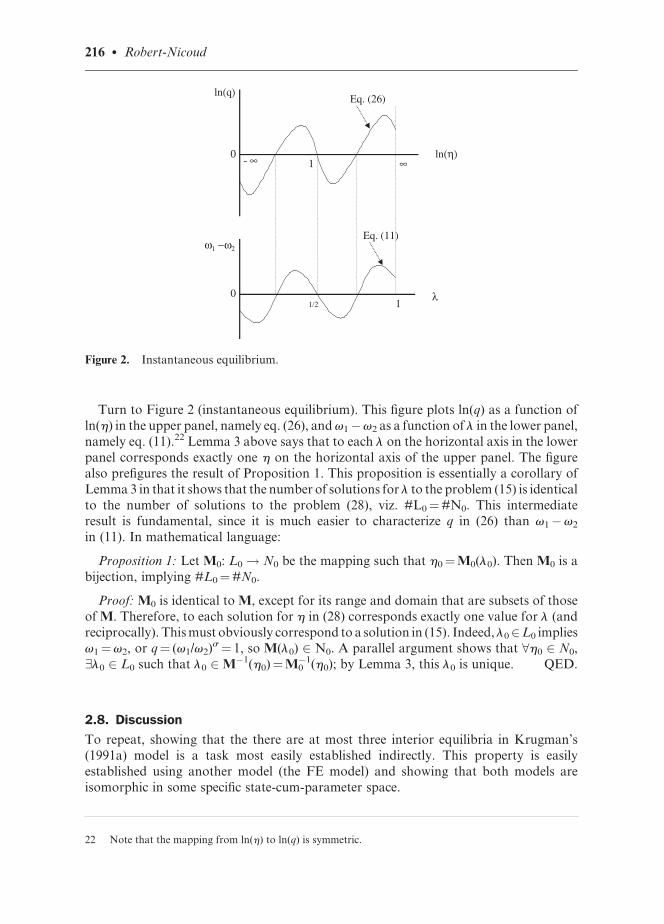
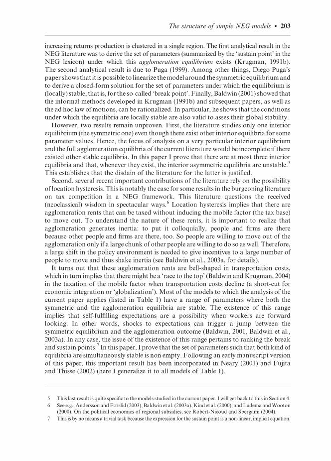
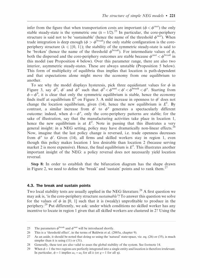
Turn to Figure 2 (instantaneous equilibrium). This figure plots ln(q) as a function of

ln(h) in the upper panel, namely eq. (26), and v1�v2 as a function of l in the lower panel,

namely eq. (11).22 Lemma 3 above says that to each l on the horizontal axis in the lower

panel corresponds exactly one h on the horizontal axis of the upper panel. The figure

also prefigures the result of Proposition 1. This proposition is essentially a corollary of

Lemma 3 in that it shows that the number of solutions for l to the problem (15) is identical

to the number of solutions to the problem (28), viz. #L0¼#N0. This intermediateresult is fundamental, since it is much easier to characterize q in (26) than v1�v2

in (11). In mathematical language:

Proposition 1: Let M0: L0 ! N0 be the mapping such that h0¼M0(l0). Then M0 is a

bijection, implying #L0¼#N0.

Proof: M0 is identical to M, except for its range and domain that are subsets of those

of M. Therefore, to each solution for h in (28) corresponds exactly one value for l (and

reciprocally). This must obviously correspond to a solution in (15). Indeed, l02L0 impliesv1¼v2, or q¼ (v1/v2)s ¼ 1, so M(l0) 2 N0. A parallel argument shows that 8h0 2 N0,

9l0 2 L0 such that l0 2 M�1(h0)¼M0�1(h0); by Lemma 3, this l0 is unique. QED.

2.8. Discussion

To repeat, showing that the there are at most three interior equilibria in Krugman’s

(1991a) model is a task most easily established indirectly. This property is easily

established using another model (the FE model) and showing that both models are

isomorphic in some specific state-cum-parameter space.

ln(η)

λ

- ∞

0

ω1 −ω2

1/2 1

1 ∞

ln(q)Eq. (26)

Eq. (11)

0

Figure 2. Instantaneous equilibrium.

22 Note that the mapping from ln(h) to ln(q) is symmetric.


In this section, Proposition 1 established that there is a one-to-one mapping between thesolution sets in the two state spaces for Krugman’s CP model. In the terms of the ‘natural’

state-cum-parameter space, we are left showing that the curve q� 1 plot against h crosses

the horizontal axis at most thrice, a case Figure 1 illustrates. A sufficient condition for this

to be true is that the curve q� 1 admits at most two flat points when plotted against l or h.

Showing this directly proved to be a task beyond the reach of my patience. Rather, there

is a more elegant—albeit indirect—way of doing it. This method first involves showing

that the alternative model of migration-driven agglomeration, the FE model, can be fully

described by the system in (26); in other words, the FE and CP models are isomorphic.This is a key result of the paper in itself.

Moreover, the FE model does admit at most three interior equilibria so this property

immediately applies to the CP model as well.

These two results are formally established in Propositions 2 and 3 of the following

section.

3. The Footloose entrepreneur model

The goal here is to derive the characteristics of the set of instantaneous equilibria of the FE

model so as to export them into the CP model. Theoretically, in this section I could followall the steps of the previous section to show how the instantaneous equilibrium of this

alternative model based on factor migration can be rewritten as (26). (The law of motion

and the long run equilibrium are still depicted by (14) and (28), respectively.) In fact, I will

only point to the differences between the two models, implying that whenever I am being

silent about a variable or a parameter it remains defined as in the previous section.

In the FE model, skilled workers are specific to the M-sector, but unskilled workers are

employed in both sectors; specifically, the cost function is no-longer homothetic as in (2)

but takes the following functional form instead:

CðxðiÞÞ ¼ wF þ wU rxðiÞ ð29Þ

where wU is the unskilled labor wage rate and is equal to unity by our choices of units and

normalizations.23 That is, the unskilled wage is equal to 1 because the A-sector transforms

one unit of unskilled labour into one unit of A (the numeraire) under perfect competitionand its output is freely traded. Since the M sector also uses unskilled workers as the

sole variable inputs, the optimal prices are now function of the parameters only. Hence, (5)

has to be replaced by:

pjðiÞ ¼r

1 � 1=s¼ 1; pkðiÞ ¼

r

1 � 1=sT ¼ T , k 6¼ j ð30Þ

and the following expressions have to be updated accordingly. The key to the tractability

of this model is that the definition of the price indices and the wages equations are no-

longer recursive. Before substantiating that claim, we have to make one more change.

23 This apparently innocuous change has a strong implication: in the CP model, the size of firms is fixed by free-entry and the variable of adjustment is the number of firms; in the FE model, exactly the opposite is true(specifically, the number of firms varies with the prevailing nominal wage). Nevertheless, the two models areisomorphic.


3.1. Normalizations

We keep all the normalizations of the CP model, but one. We take:

Labour endowments: LU=L ¼ ðs � mÞ=m;

so that (16) holds as before (again, this normalization implies that nominal wages are

equalized throughout at any stable long run equilibrium).

3.2. Instantaneous equilibrium in the FE model

Step 6: I now show that the CP and FE models are isomorphic in the natural state space.

Following the same steps as is the previous section, it is clear that (10) still holds. However,

the instantaneous equilibrium is now being characterized by the following set of

equations:

Y1 ¼ mlw1

sþ s � m

2s, Y2 ¼ mð1 � lÞw2

sþ s � m

2s

G1�s1 ¼ l þ ð1 � lÞf, G1�s

2 ¼ lf þ ð1 � lÞ

w1 ¼ Y1

G1�s1

þ fY2

G1�s2

, w2 ¼ fY1

G1�s1

þ Y2

G1�s2

ð31Þ

This is a simpler model in that the price-indices now depends on l and f only—in

particular, they depend on no ‘short-run’ endogenous variable; this way explicit

solutions for v1 and v2 are available (see Forslid and Ottaviano 2003 and Appendix 1in the present paper).

By virtue of (16), we can define h as the ratio of the mobile factor’s expenditure in 1 to

mobile expenditure in 2, as before (19). Also, f is still defined by (17) and x is still defined

by (20); with the new normalization, we have x ¼ (s �m)/(s þm). Also, the parameter

capturing the forward linkages (21) has to be redefined as:

u � m

s � 1ð32Þ

The interpretation of u and the no-black-hole condition u< 1 remain the same. Finally,

the definition of q (25) has to be replaced by:

q � v1

v2ð33Þ

As an aside, and to ease the step from (31) to (35), note that (12), (19), and (24) together

imply:

v ¼ G1

G2

� �m

h1 � l

lð34Þ

Now, solve for l/(1� l) and plug the result into (31); use also the definition of Dj (23) and

the ratio notation to get:

Y ¼ h þ x

1 þ hx; hDu ¼ q

D� f

1 � Df; q ¼ Du Y þ Df

Yf þ Dð35Þ


Thus we have shown the first central result of this paper:

Proposition 2: The CP and FE model are isomorphic in the natural state space.24

Proof: Clearly, (35) and (26) are identical, hence the CP and FE models are isomorphic.

QED.

Consequently, we can use Figure 2 for the FE model, too, in which case the bottom and

upper panels correspond to Eq. (31) and Eq. (35), respectively. We define the set of interior

long run solutions to (35) for h and l as N0FO and L0

FO, respectively:

NFO0 � fh > 0 : f ð1, hÞ ¼ 0g, LFO

0 � fl > 0 : FFOð0, lÞ ¼ 0g ð36Þ

these are the equivalent of N0 in (28) and L0 in (15).

At this stage it is worth pausing to get the intuition for the remainder of the proof of the

main result in this paper (Proposition 3 below). Since (35) is identical to (26), the sets N0

and N0FO are identical as well, though generically the sets L0 and L0

FO are not. (In

particular, asymmetric steady-states differ). What is important, however, is that thenumber of steady states in each model is identical.

Step 7: A final intermediate result is needed before we can turn to the proof proper:

Lemma 4: The FO model admits at most 3 interior steady-states, viz. #L0FO � 3.


We have at last everything at hand to prove the main result of this paper, namely that

#L0 is no larger than 3 for the CP model as well.

4. On the number of steady-states and location hysteresis

This section contains the remaining results of the paper. Proposition 3 establishes that

the CP model admits at most three interior steady-states and that location hysteresis

happens for some parameter values. Proposition 4 proves that the existence of forward

linkages is a prerequisite to the possibility of equilibrium switching generated by

shocks to expectations; of course, this can only happen in versions of the model in

which agents are forward-looking, as in Baldwin (2001) and Ottaviano (2001). Finally,

Proposition 5 establishes that asymmetric interior steady-states are always unstable(if they exist at all).

4.1. Threshold effects, hysteresis, and shocks to expectations

Technically speaking, location displays hysteresis whenever several stable equilibriacoexists under the same parameter values. In the current models, there is a region in

the parameter space (to be defined precisely shortly) under which two equilibria are

(locally and globally) stable: the agglomeration equilibrium where agglomeration

occurs in region 1 and the agglomeration equilibrium where agglomeration occurs in

region 2. Given the law of motion (14), it is clear that location is path dependent. This form

24 Appendix 2 shows that the FCVL model is also a perfect twin of the CP and FE models.


of hysteresis is sufficient to generate agglomeration rents that are at the core of theliterature on NEG and tax competition; see Baldwin et al. (2003a, Part IV) for a

comprehensive analysis.

In the current models, there even exists a region of the parameter space for which

the symmetric and agglomeration equilibria are all three stable. This configuration

is interesting because it means that two spatial configurations very different in

nature—full spatial dispersion and concentration—can emerge as a long run

equilibrium. It also implies that shocks to expectations may trigger an equilibrium

switch (that is to say, the basins of attraction of several steady-states overlap; seeBaldwin, 2001). The models of Baldwin (1999) and Ottaviano et al. (2002) do not

exhibit this property.

It is useful to start by determining the generic number of steady-states.

4.2. On the number of steady-states

The next proposition is the second central result of this paper.

Proposition 3: The CP model admits at most three interior steady-states.

Proof: Start with the FE model. Using Lemmas 3 and 4, we have #N0FO � 3. Since

the (26) is identical to (35), it must be that N0¼N0FO. Invoking Proposition 1, we

find #L0¼#N0¼#N0FO¼#L0

FO. This implies #L0 � 3 and establishes the result.

QED.

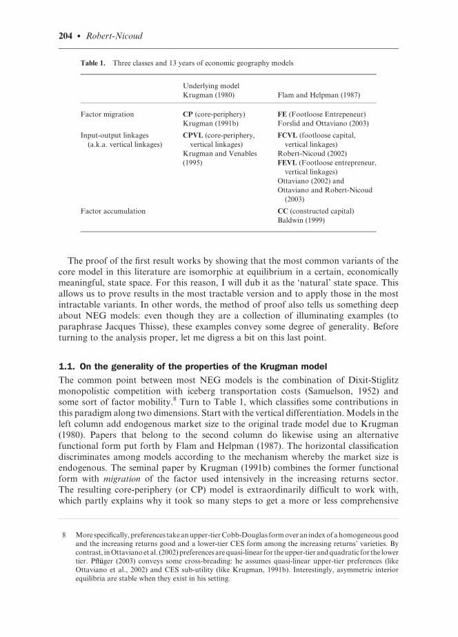
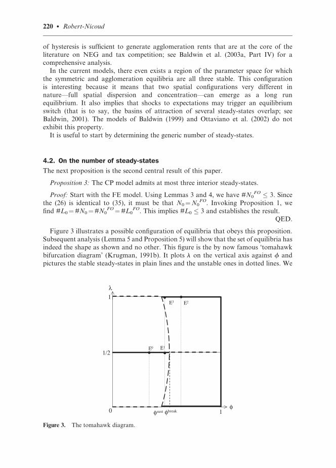
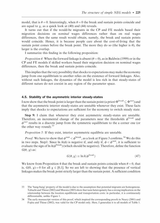
Figure 3 illustrates a possible configuration of equilibria that obeys this proposition.

Subsequent analysis (Lemma 5 and Proposition 5) will show that the set of equilibria has

indeed the shape as shown and no other. This figure is the by now famous ‘tomahawk

bifurcation diagram’ (Krugman, 1991b). It plots l on the vertical axis against f and

pictures the stable steady-states in plain lines and the unstable ones in dotted lines. We

1/2

φ

λ

0

1

1φbreakφsust

Ε1Ε0

Ε2Ε3

Figure 3. The tomahawk diagram.


infer from the figure that when transportation costs are important (f<fsust) the onlystable steady-state is the symmetric one (l¼ 1/2).25 In particular, the core-periphery

structure is said not to be ‘sustainable’ (hence the name of the threshold fsust). When

trade integration is deep enough (f > fbreak) the only stable configuration is the core-

periphery structure (l 2 |{0, 1}); the stability of the symmetric steady-state is said to

be ‘broken’ (hence the name of the threshold fbreak). For intermediate values of f,

both the dispersed and the core-periphery outcomes are stable because fsust<fbreak in

this model (see Proposition 4 below). Over this parameter range, there are also two

interior, asymmetric steady-states. These are always unstable (Proposition 5 below).This form of multiplicity of equilibria thus implies that location is path-dependent

and that expectations alone might move the economy from one equilibrium to

another.

To see why the model displays hysteresis, pick three equidistant values for f in

Figure 3, say f0, f0 and f00 such that f0<fsust<f0 <fbreak <f00. Starting from

f¼f0, it is clear that only the symmetric equilibrium is stable, hence the economy

finds itself at equilibrium E0 on Figure 3. A mild increase in openness to f0 does not

change the location equilibrium, given (14), hence the new equilibrium is E1. Bycontrast, a similar increase from f0 to f00 generates a spectacularly different

outcome: indeed, when f¼f00, only the core-periphery patterns are stable; for the

sake of illustration, say that the manufacturing activities take place in location 1,

hence the new equilibrium is at E2. Note in passing that this illustrates a very

general insight: in a NEG setting, policy may have dramatically non-linear effects.26

Now, imagine that the last policy change is reversed, i.e. trade openness decreases

from f00 to f0. Given (14), all firms and skilled workers stay in region 1, even

though this policy makes location 1 less desirable than location 2 (because servingmarket 2 is more expensive). Hence, the final equilibrium is E3. This illustrates another

important insight of the NEG: a policy reversal does not necessarily yield location

reversal.

Step 8: In order to establish that the bifurcation diagram has the shape drawnin Figure 2, we need to define the ‘break’ and ‘sustain’ points and to rank them.27

4.3. The break and sustain points

Two local stability tests are usually applied in the NEG literature.28 A first question wemay ask is, ‘is the core-periphery structure sustainable’? To answer this question we solve

for the values of f in [0, 1] such that it is (weakly) unprofitable to produce in the

periphery.29 Put differently, we ask: under which conditions no skilled worker has any

incentive to locate in region 1 given that all skilled workers are clustered in 2? Using the

25 The parameters fbreak and fsust will be introduced shortly.

26 This is a ‘threshold effect’, in the terms of Baldwin et al. (2003a, chapter 9).

27 As an aside, it should be noted that doing so using the ‘natural’ state-space, viz. eq. (26) or (35), is muchsimpler than it is using (11) or (31).

28 Generally, these test are also valid to asses the global stability of the system. See footnote 14.

29 When f¼ 1 the two regions are perfectly integrated into a single entity and location is therefore irrelevant.In particular, f¼ 1 implies v1¼v2 for all l (or q¼ 1 for all h).


structural state space, this is equivalent to finding the set of values for f (call it Fsust) suchthat l¼ 0 implies v1 � v2:

Fsust � ff 2 ½0, 1� : l ¼ 0 and v1 � v2g ð37Þ

Given Proposition 3, this is the same as finding the values of f such that h¼ 0 implies

q � 1, or:

Fsust ¼ ff 2 ½0, 1� : h ¼ 0 and q � 1g ð38Þ

To answer the question above, impose h¼ 0 and q � 1 in (26) or (35). Thus (35)

becomes:

Y ¼ x; D ¼ f; 1 � Du Y þ Df

Yf þ Dð39Þ

It is readily verified that the inequality is violated for low values of f and holds trivially for

f¼ 1 As Lemma 5 below establishes, the set of (‘s such that (39) holds,Fsust, is compact

(i.e. closed and bounded). Hence, we are left finding the lowest value of f—call it fsust—such that (39) holds with equality. Solving for f, it is readily verified that the ‘sustain point’

fsust is implicitly defined as:

ð1 þ xÞðfsustÞ1�u � ðfsustÞ2 � x ¼ 0 ð40Þ

To be more precise, fsust is the lowest root of the above polynomial (f¼ 1 is the

other real root). This expression holds for the CP and the FE models alike (remember,

they are isomorphic by Proposition 2). The corner steady-states are stable whenever

f � fsust.

We may also ask an alternative question: When is the symmetric equilibrium unstable?Answering this question involves signing the first derivative of v1�v2 at l¼ 1/2 in the

structural state space or the first derivative of ln(q) with respect to ln(h) in the natural state

space.30 The economic rationale for asking this question is as follows. Start with the

symmetric equilibrium (in which real wages are always equalized) and imagine that a

shock were to perturb this equilibrium slightly in the form of moving ‘one’ skilled worker

from region 2 to region 1. If the resulting real wage in 1 is larger than in 2, then the initial

shock is destabilizing in the sense that additional skilled workers have the tendency to

leave region 2 to region 1. Thus, formally, we want to find the set of values for f (call itFbreak) such that:

Fbreak � f 2 ½0, 1� : d

dlðv1 � v2Þ

��l¼1=2

� 0

( )

¼ f 2 ½0, 1� : d

d ln hln q

��h¼1

� 0

( )ð41Þ

So let us normalize (25) around the symmetric equilibrium. In the natural state space, this

is facilitated by noting that h¼ 1 implies Y¼D¼ q¼ 1 because of the symmetry of the

model and by definition of the ratio variables (24). This is handy because in that case d ln

h¼ dh, d ln Y¼ dY, d ln D¼ dD and d ln q¼ dq. Given this, it is straightforward to show

30 This first-order approximation technique was introduced by Puga (1999).


that total differentiation of the system in (35) can be written in matrix form as:

1 0 0

0 u � Z�1 �1

�Z Z � u 0

24

35 dY

dD

dq

24

35 ¼

ð1 � xÞ=ð1 þ xÞ�1

0

24

35dh; Z � 1 � f

1 þ fð42Þ

(where is Z is monotonically decreasing in f, with Z¼ 0 if f¼ 1 and Z¼ 1 if f¼ 0).

Applying Cramer’s rule on (42), we find:

0 � dq

dh� �Z

Zðu � Z�1Þð1 � xÞ þ ðZ � uÞð1 þ xÞð1 � Z2Þð1 þ xÞ

¼ �Z2½uð1 � xÞ þ ð1 þ xÞ� þ Zð1 � xÞ þ uð1 þ xÞ�ð1 � Z2Þð1 þ xÞ ð43Þ

The numerator of the last expression above is quadratic in Z and, clearly, Z¼ 0 (f¼ 1) is

one root of this polynomial. (As we shall see in Lemma 5, Fbreak is compact and includes

1.) Hence, we are left finding a lower bound for this set and hence to find the value of f< 1

such that the inequalities in (41) and (43) hold with equality.

Define the non-zero root of this second-order polynomial for Z > 0 as Zbreak. The

corresponding value for f is:31

fbreak � x1 � u

1 þ uð44Þ

which is in (0,1) by the no black-hole and the lumpy-feet conditions. The symmetricsteady-state is unstable whenever f � fbreak

Using the definitions of x and u, (40) and (44) are of course equivalent to Eq. (5.17) and

Eq. (5.28) in Fujita et al. (1999, pp.70, 74) and Eqs. (25) and (26) in Forslid and Ottaviano

(2003). I sum up these results in the following Lemma. (Part of its proof is needed for

Proposition 4, hence I develop it in the main text rather than in the appendix.)

Lemma 5: The sets Fsust and Fbreak are compact.

Proof: Start with Fbreak. Clearly, the numerator of the last expression in (43) is concavein Z everywhere on the unit interval. Also, it is nil when Z¼ 0 and negative when Z � 1.

Hence, the set of Z’s for which the inequality in (43) is satisfied is compact. Since Z(.) is a

monotonic transformation of f, Fbreak is also compact. Turn now to Fsust. To this end, I

characterize how the natural logarithm of the function hðfÞ � ½f2 þ x�=½f1�uð1 þ xÞ,which is just a transformation of (40), changes with f.32 In particular, ln(h) and the

left-hand side of (40) have the same zeroes. Given this, we have:

ln hðfÞ ¼ lnðf2 þ xÞ � ð1 � uÞ ln f � lnð1 þ xÞd

dfln hðfÞ ¼ 2f

f2 þ x� 1 � u

f

d2

df2ln hðfÞ ¼ 2ðx � f2Þf2 þ ð1 � uÞðf2 þ xÞ2

f2ðf2 þ xÞ2

ð45Þ

31 For computational purposes, note that f¼ (1�Z)/(1þZ) by definition of Z.

32 As Baldwin et al. (2003a) show, h(�) has an economic interpretation as the inverse of agglomeration rents.


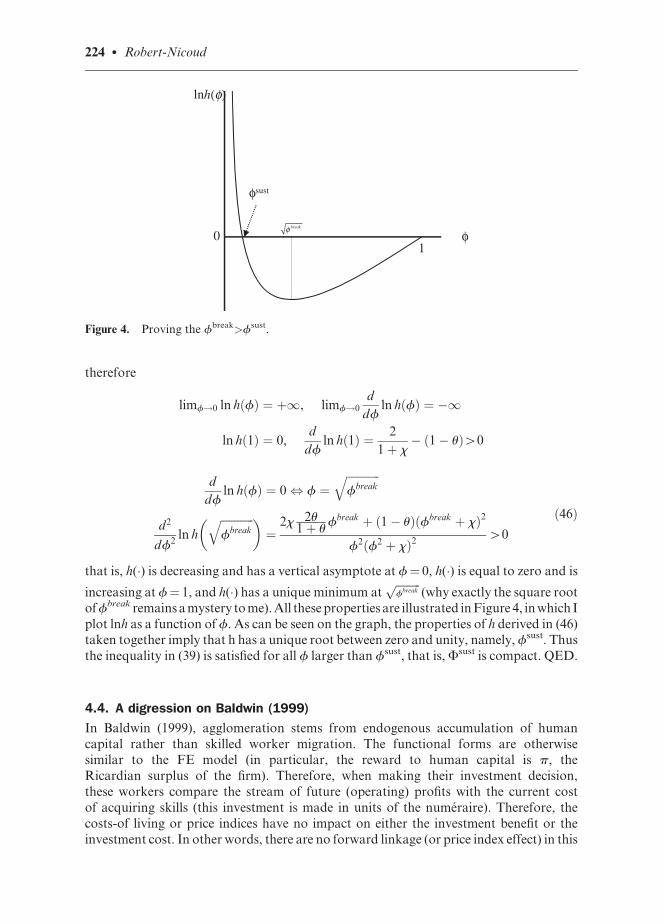
therefore

limf!0 ln hðfÞ ¼ þ1, limf!0d

dfln hðfÞ ¼ �1

ln hð1Þ ¼ 0,d

dfln hð1Þ ¼ 2

1 þ x� ð1 � uÞ40

d

dfln hðfÞ ¼ 0 , f ¼

ffiffiffiffiffiffiffiffiffiffiffiffifbreak

q

d2

df2ln h

ffiffiffiffiffiffiffiffiffiffiffiffifbreak

q� ¼

2x 2u1 þ u

fbreak þ ð1 � uÞðfbreak þ xÞ2

f2ðf2 þ xÞ240

ð46Þ

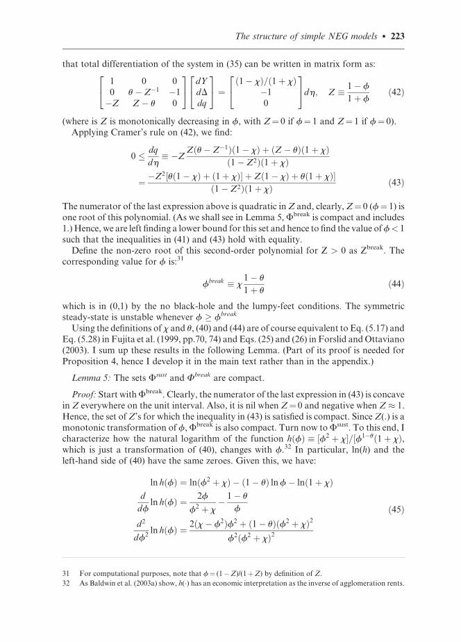
that is, h(�) is decreasing and has a vertical asymptote at f¼ 0, h(�) is equal to zero and is

increasing at f¼ 1, and h(�) has a unique minimum atffiffiffiffiffiffiffiffiffifbreak

p(why exactly the square root

of fbreak remains a mystery to me). All these properties are illustrated in Figure 4, in which I

plot lnh as a function of f. As can be seen on the graph, the properties of h derived in (46)taken together imply that h has a unique root between zero and unity, namely, fsust. Thus

the inequality in (39) is satisfied for all f larger than fsust, that is, Fsust is compact. QED.

4.4. A digression on Baldwin (1999)

In Baldwin (1999), agglomeration stems from endogenous accumulation of human

capital rather than skilled worker migration. The functional forms are otherwisesimilar to the FE model (in particular, the reward to human capital is p, the

Ricardian surplus of the firm). Therefore, when making their investment decision,

these workers compare the stream of future (operating) profits with the current cost

of acquiring skills (this investment is made in units of the numeraire). Therefore, the

costs-of living or price indices have no impact on either the investment benefit or the

investment cost. In other words, there are no forward linkage (or price index effect) in this

φ01

lnh(φ)

φsust

breakφ

Figure 4. Proving the fbreak>fsust.


model, that is u¼ 0. Interestingly, when u¼ 0 the break and sustain points coincide andare equal to x, as a quick look at (40) and (44) reveals.

It turns out that if the would-be migrants in the CP and FE models based their

migration decisions on nominal wages differences rather than on real wages

differences, then the same result would obtain, namely, the break and sustain points

would coincide. Hence, it is because people care about the cost-of-living that the

sustain point comes before the break point. The more they do so (the higher is u), the

larger is the overlap.

I summarize this finding in the following proposition:

Proposition 4: When the forward linkage is absent (u¼ 0), as in Baldwin (1999) or in the

CP and FE models if skilled workers based their migration decision on nominal wages

differences, then the break and sustain points coincide.

This implies that the very possibility that shocks to expectations may make the economy

jump from one equilibrium to another relies on the existence of forward linkages. Also,

without such linkages, the dynamics of the model is less rich in that steady-states of

different nature do not coexist in any region of the parameter space.

4.5. Stability of the asymmetric interior steady-states

I now show that the break point is larger than the sustain point (a prioriFbreak�Fsust) and

that the asymmetric interior steady-states are unstable whenever they exist. These factsimply that shocks to expectations are sufficient for the economy to switch steady state.

Step 9: I claim that whenever they exist asymmetric steady-states are unstable.

Therefore, an incremental change of the parameters near the thresholds fbreak and

fsust results in a discrete jump from the symmetric equilibrium to the a corner one (orthe other way round).33

Proposition 5: If they exist, interior asymmetric equilibria are unstable.

Proof: We have to show that fsust<fbreak, as a look at Figure 3 confirms.34 We do this

in two steps. Step1: Since ln h(f) is negative if, and only if, f<fsust, it is sufficient to

evaluate the sign of ln h(fbreak) (which should be negative). Therefore, define the function

G(u, x) as:

Gðu, xÞ � ln hðfbreakÞ ð47Þ

We know from Proposition 4 that the break and sustain points coincide when u¼ 0, that

is, G(0, x)¼ 0 for all x 2 [0,1]. So we are left to showing that the presence of vertical

linkages makes the break point strictly larger than the sustain point. A sufficient condition

33 The ‘bang-bang’ property of the model is due to the assumption that potential migrants are homogenous.Tabuchi and Thisse (2002) and Murata (2003) show that taste heterogeneity has a strong implication on therelationship between the location equilibrium and transportation costs: in particular, it is continuouslydifferentiable, unlike Figure 1.

34 The early manuscript version of this proof, which inspired the corresponding proofs in Neary (2001) andFujita and Thisse (2002), was valid for the CP model only. Here, I generalize it to all models of Table 1.


for this to be true is that @G/@u � 0 holds for all x and u in [0,1]. Step 2: To this aim, notethat G(., x) is concave:

d2

du2Gðu, xÞ ¼ �4

1 þ u

1 � u� x

� 1 þ u

1 � u

� 2

�x

" #

ð1 þ uÞð1 � uÞ2 1 þ u

1 � u

� 2

þx

" #250 ð48Þ

because 0< x, u< 1. Hence, a sufficient condition for G(., x)�0 to hold is G(0, x)¼ 0

(which we know to be true from Proposition 4) and the first derivative of G with respect

to u to be non-positive when evaluated at u¼ 0. This is indeed the case, as I now show.

Define:

g0ðxÞ �d

duGðu, xÞ

��u¼0

¼ @

@fln hðf; uÞ

��f¼fbreak

d

dufbreak

��u¼0

þ @

@uln hðu; fÞ

��f¼fbreak, u¼0

ð49Þ

Using (44) and (45), it takes little algebra to see that g0(x) � 0 holds for all x in [0, 1]:

g0ðxÞ ¼ 21 � x

1 þ xþ ln x � 0 ð50Þ

To get the inequality above, note that g0(x) is concave on [0, 1] and that both g0¼ 0 and

@g0=@x ¼ 0 hold when x ¼ 1.35 These facts imply that G(u, x) is non-positive over the

whole parameter space. The point of all this is that the upper bound of G(u, x), and thus theupper bound of h(fbreak), is zero. We know, therefore, that for all permissible values of x

and u, fsust � fbreak, as claimed. QED.

This completes the proof and implies that the asymmetric interior steady-states areunstable.

4.6. Further discussion

As we saw, without forward linkages (or price-index effect), the break and sustain points

coincide. This is not a general result. To see this, note first that the break point without

forward linkage is defined as the (limiting) set of parameter for which a marginalmigration raises the nominal wage in the host region and decreases it in the source

region; that is, we are talking about signing a first derivative. Second, the sustain

point without forward linkage is defined as the (limiting) set of parameters for which

the nominal wages are larger in region 1 than in region 2 if and only if all mobile workers

are settled in region 1; that is, we are talking about a difference in levels. There is no reason

a priori why these two limiting values should coincide. In fact, they do so in the present

setting because of Cobb-Douglas preferences in particular. Adding the price-index effect

35 I am grateful to Maarten Bosker who pointed out to me that a previous version of this paper containedalgebraic mistakes in (49) and (50) (CEPR discussion paper no. 4326). Though these mistakes requiredminor alterations to those expressions, these alterations do not change the inequalities in (49) and (50).


to this setting results in the sustain point coming before the break point. In sharp contrast,Pfl€uuger (2003) shows that the break point comes before the sustain point when preferences

are quasi-linear (linear in A and logarithmic in M).

Closer to the actual setting, Puga (1999) shows that the ‘bang-bang’ property of the

model occurs because wage costs do not rise fast enough when firms are clustering. To

understand the mechanism at work, start at the symmetric equilibrium. Now imagine that

the parameters of the model take values so that f > fbreak. When the first firm moves out

of the symmetric equilbrium, wage costs increase by less than revenue for equal real wages

so the move is worthy (Puga 1999 has shown that this alternative way of modeling thedynamics of the model yields the same analytical results). Hence, a second firm follows

suit; this, too, is worthy, and so on, all the way to full agglomeration (because no stable

asymmetric equilibrium exists).

When the local labour supply is relatively inelastic then this ‘bang-bang’ property may

vanish. In Krugman and Venables (1995), manufacturing (or skilled) workers are

immobile across regions and must be pulled from the traditional A sector. In Puga

(1999), skilled workers can also move across regional borders, like in the CP and FE

models. The point in the Krugman, Venables and Puga settings being that, if there aredecreasing returns in labour in the A sector, then manufacturing firms face an less-than-

fully elastic labour supply.

This has two important consequences. First, the agglomerated steady state is no longer

stable when transportation costs are very low. To see this, observe that nominal wages are

much higher in the region in which the manufacturing sector is clustered than in the

periphery because skilled labour demand is higher in the former than in the latter. If some

firms were to locate in the periphery, they would have nearly as good an access to the large

market in the core than firms located there (when transportation costs are low) but withmuch lower labour costs. Hence, the agglomeration equilibrium is sustained for

intermediate values of f only (it can be shown that Fsust and Fbreak both remain

compact, though they no longer include 1). In terms of Figure 3, and assuming that

the ‘bang-bang’ properties of the model are unaffected, the diagram would look like a

double-edged tomahawk.

The second important consequence is that these bang-bang properties may disappear

altogether. Indeed, when firms are clustering wage costs might rise fast enough in a way

that makes the location equilibrium a smooth function of f (with the asymmetricequilibria now being stable). In terms of Figure 3, the diagram would look like a

double-pitchfork instead. Whether it takes the shape of a double-pitchfork or a

double-tomahawk depends on the parameter values of the model.

5. Concluding remarks

This paper has shown that the original core-periphery (CP) model by Krugman (1991a,b)

and the alternative footloose entrepreneur (FE) model by Forslid and Ottaviano (2003)

can be entirely characterized by the same set of equations in the appropriate state-cum-

parameter space; in other words, the CP and FE models are isomorphic—indeed,expressions (26) and (35) are identical. An implication of this fact is that it is sufficient

to describe the properties of either model to know the stability properties of both. This is

the strategy that I have pursued in this paper. It is worth emphasizing that the natural state

variable of these models is mobile expenditure. This implies that the relevant variable to


look at in empirical studies (at least those explicitly based on NEG models) is the spatialdistribution of expenditure or income of mobile factors (rather than population).

In both the CP and the FE models agglomeration is driven by (skilled) labour

migration. Other agglomeration mechanisms have been put forward, too. On the one

hand are the models based on input-output (or ‘vertical’) linkages among firms. The

‘footloose-capital’ model with vertical linkages (FCVL model in Table 1) developed in

Robert-Nicoud (2002) is isomorphic to the CP and FE models, hence the proof developed

in this paper generalizes to that model as well, as Appendix 2 shows. However, the original

model with vertical linkages (see e.g., Fujita et al., 1999, section 14.2), referred to as theCPVL model in Table 1 (CPVL stands for ‘core-periphery, vertical linkages’), has two

state variables, not one (as does its tractable cousin, the FEVL due to Ottaviano, 2002).

Indeed, in this model factor owners are immobile across regions but labour moves from

one sector to the other so that nominal wages are equalized within each region and across

sectors. As it turns out, a simple extension of the method developed in this paper allows an

exhaustive analysis of the equilibrium properties of the CPVL model, but this would take

us too far apart here (remarkably, (26) drives the behaviour of one state variable in both

the CPVL and FEVL models). The interested reader can refer to Ottaviano and Robert-Nicoud (2003) for details.

On the other hand are models based on factor accumulation; the simplest among these

models (Baldwin, 1999) can be written as a special case of (26)—specifically, u¼ 0. This

implies that this model generically admits at most one interior equilibrium—the

symmetric one. Hence, the break and sustain point coincide. (The methodology

developed in this paper can be used to show both of these facts but it is much easier

to show these more directly; see Baldwin, 1999.)

5.1. Common features of popular NEG models

Given that all these models are isomorphic (and nearly identical), it is unsurprising that

they all share the same features. Here are some of them. First, location displays hysteresis

when transportation costs are low enough (i.e. when trade openness, as parameterized by

f, is large enough). Specifically, agglomeration is self-sustaining so that it generates

location-specific economic rents. These rents can be taxed to some extend without

loosing the tax base, a fact that the new literature on taxation of mobile factorsexploits intensively. Second, policy potentially has very non-linear effects. In the

ex ante symmetric region-case that the NEG typically assumes, policy has no impact

on location unless it goes beyond some threshold. When it does so, the impact is

spectacular and discrete (typically the equilibrium jumps from a symmetric outcome

to a core-periphery one or the other way round). Finally, since all the models of

Table 1 but one (Baldwin, 1999) have a range of parameters where both the

symmetric and the agglomeration equilibria are stable, shocks to expectations can

generate a jump between the symmetric equilibrium and the agglomeration outcomewhen migrants are forward looking.

5.2. Implications for empirical work

The threshold and hysteresis results have stark implications for empirical work (Baldwin

et al., 2003a). First, policy potentially has non-linear effects, hence empirical studies that

impose linearity are potentially miss-specified. Second, past experience can be a poor


guide to assess the effect of a particular policy. Also, a bad policy might not easilybe reverted if there are ‘lock-in’ (hysteresis) effects—but see Davis and Weinstein

(2002, 2004).

Moreover, as we saw at great lengths, all NEG models of Table 1 are isomorphic

irrespective of the agglomeration mechanism they are assuming. This in itself brings

good and bad news alike for the empirical work. The good news first. The predictions

of the model are robust to the assumption about the underlying agglomeration

mechanism. This implies that the results of an empirical investigation based on the

reduced form of any model are more general and could be derived from any otherstructural model, the only difference being in the interpretation of the structural

parameters. This conveys bad news, too, because under these conditions it is at best

very difficult to identify the channel by which agglomeration operates. In particular,

all three mechanisms listed in the rows of Table 1 probably play a role in the real

world. Since they all show up the same way in the reduced form, it might be difficult

to assess the magnitude of their respective roles.

It is my hope that the present paper is helpful in understanding why these models are so

strikingly similar and how the agglomeration and dispersion forces interact in such a waythat no more than five steady-states ever exist. Common functional forms are necessary

for the isomorphism result. However, it is extremely remarkable that they are sufficient as

well, since the mechanisms driving agglomeration differ from one model to the next, as

does the interpretation of the parameters. This allows for some cautious optimism as for

the generality of the predictions of the NEG theory in its current form.

Acknowledgements

I am very grateful to Richard Baldwin, Gilles Duranton, and Diego Puga for suggestions thatgreatly improved the structure of the paper (Diego Puga’s written summary was so apt that Iincorporated part of it in the text almost verbatim), as well as to Maarten Bosker, Rod Falvey,Yasu Murata, Federica Sbergami, and Takatoshi Tabuchi for useful comments. I also thank CarloFiorio, Fredrik Gallo, Steve Redding, Jacques Rougemont, Jacques Thisse, Federico Trionfetti,and Tony Venables for fruitful discussions at various stages of this paper. Usual disclaimers apply.This paper is a revised version of chapter 2 of my PhD thesis at the LSE and was part of theglobalization program at the ESRC-founded Centre for Economic Performance at the LSE. I amgrateful to both of these institutions for their material and financial support, respectively.

References

Andersson, F., Forslid, R. (2003) Tax competition and economic geography. Journal of PublicEconomic Theory, 5(2): 279–304.

Baldwin, R. E. (1999) Agglomeration and endogenous capital. European Economic Review, 43(2):253–280.

Baldwin, R. E. (2001) The core-periphery model with forward looking expectations. RegionalScience and Urban Economics, 31: 21–49.

Baldwin, R. E., Forslid, R., Martin, P., Ottaviano, G.I.P., Robert-Nicoud, F. (2003a) EconomicGeography and Public Policy. Princeton, NJ: Princeton University Press.

Baldwin, R. E., Forslid, R., Martin, P., Ottaviano, G.I.P., Robert-Nicoud, F. (2003b) The core-periphery model: key features and effects. In B. Heijdra and S. Blackman (eds) The MonopolisticCompetition Revolution in Retrospect. Cambridge: Cambridge University Press.

Baldwin, R. E., Martin, P., Ottaviano, G. I. P. (2001) Global income divergence, trade, andindustrialization: the geography of growth take-offs. Journal of Economic Growth, 6: 5–37.


Baldwin, R. E., Krugman, P. (2004) Agglomeration, integration and tax harmonization. EuropeanEconomic Review, 48(1): 1–23.

Charlot, S., Gaigne, C., Robert-Nicoud, F., Thisse, J. F. (2003) Agglomeration and welfare: the core-periphery model in the light of Bentham, Kaldor, and Rawls. Discussion paper no. 2003/39,CORE, Louvain-la-Neuve; and Discussion paper, CEPR, London, forthcoming.

Davis, D., Weinstein, D.E. (2002) Bones, bombs and break points: the geography of economicactivity. American Economic Review, 92(5): 1269–1289.

Davis, D., Weinstein, D.E. (2004) A search for multiple equilibria in urban industrial structure.Working paper no. 10252, NBER, Cambridge, MA.

Flam, H., Helpman, H. (1987) Industrial policy under monopolistic competition. Journal ofInternational Economics, 22: 79–102.

Faini, R. (1984) Increasing returns, non-traded inputs and regional development. EconomicsJournal, 94: 308–323.

Forslid, R., Ottaviano, G. I. P. (2003) An analytically solvable core-periphery model. Journal ofEconomic Geography, 3: 229–240.

Fujita, M., Krugman, P., Venables, A. J. (1999) The Spatial Economy. Cambridge, MA: MIT Press.Fujita, M., Thisse, J. F. (2002) Economics of Agglomeration. Cambridge: Cambridge University

Press.Head, K., Mayer, T. (2004) The empirics of agglomeration and trade. In J.V. Henderson and

J.F. Thisse (eds) Handbook of Urban and Regional Economics. Amsterdam: North Holland.Helpman, H., Krugman, P. (1985) Market Structure and Foreign Trade. Cambridge, MA: MIT Press.Jones, R. W. (1965) The structure of simple general equilibrium models. Journal of Political

Economy, 73: 557–572.Kind, H., Midelfart Knarvik, K.H., Schjelderup, G. (2000) Competition for capital in a lumpy

world. Journal of Public Economics, 78(3): 253–74.Krugman, P. (1980) Scale economies, product differentiation and the pattern of trade. American

Economic Review, 70: 950–959.Krugman, P. (1991a) Geography and Trade. Cambridge, MA: MIT Press.Krugman, P. (1991b) Increasing returns and economic geography. Journal of Political Economy, 99:

483–499.Krugman, P. (1991c) History versus expectations. Quarterly Journal of Economics, 106 (2):

651–667.Krugman, P., Venables, A. J. (1995) Globalization and the inequality of nations. Quarterly Journal

of Economics, 110(4): 857–880.Ludema, R., Wooton, I. (2000) Economic geography and the fiscal effects of regional integration.

Journal of International Economics, 52(2): 331–335.Maffezzoli, M., Trionfetti, F. (2002) Approximation methods: and application to the core-periphery

model. Mimeo, IGIER and CEPN.Matsuyama, K. (1991) Increasing returns, industrialization, and indeterminacy of equilibrium.

Quarterly Journal of Economics, 106(2): 617–650.Matsuyama, K. (1995) Complementarities and cumulative processes in models of monopolistic

competition. Journal of Economic Literature, 33: 701–729.Matsuyama, K., Takahashi, T (1998) Self-defeating regional concentration. Review of Economic

Studies, 65: 211–34.Murata, Y. (2003) Product diversity, taste heterogeneity, and geographic distribution of economic

activities: market vs. non-market interactions. Journal of Urban Economics, 53(1): 126–144.Neary, J. P. (2001) On hypes and hyperbolas: introducing the new economic geography. Journal of

Economic Literature, 39: 536–561.Overman, H., Redding, S. J., Venables, A. J. (2003) The economic geography of trade, production

and income: a survey of empirics. In Kwan-Choi and J. Harrigan (eds) Handbook of InternationalTrade. Oxford: Basil Blackwell.

Ottaviano, G. I. P. (2001) Monopolistic competition, trade, and endogenous spatial fluctuations.Regional Science and Urban Economics, 31: 51–77.

Ottaviano, G. I. P. (2002) Models of ‘new economic geography’: Factor mobility vs. vertical linkages.Mimeo, Graduate Institute of International Studies.


Ottaviano, G. I. P., Robert-Nicoud, F. (2003) The ‘genome’ of NEG models with input-outputlinkages: a positive and normative synthesis. Mimeo, University of Bologna and University ofGeneva.

Ottaviano, G. I. P., Tabuchi, T., Thisse, J. F. (2002) Agglomeration and trade revisited. InternationalEconomic Review, 43(4): 409–436.

Ottaviano, G. I. P. and J. F. Thisse (2004) Agglomeration and economic geography. InJ. V. Henderson and J.F. Thisse (eds) Handbook of Urban and Regional Economics.Amsterdam: North Holland.

Pfl€uuger, M. (2003) A simple, analytically solvable, Chamberlian agglomeration model. RegionalScience and Urban Economics, in press.

Puga, D. (1999) The rise and fall of regional inequalities. European Economic Review, 43(2):303–334.

Robert-Nicoud, F. (2002) A simple model of agglomeration with vertical linkages and perfect capitalmobility. Chapter 1 in New Economic Geography: Welfare, Multiple Equilibria and PoliticalEconomy, PhD Thesis, London School of Economics.

Robert-Nicoud, F., Sbergami, F. (2004) Vote-market vs. home-market effects: location equilibriumin a probabilistic voting model. European Economic Review, 48(1): 155–179.

Samuelson, P. (1952) The transfer problem and transport costs: the terms of trade when impedimentsare absent. Economic Journal, 62: 278–304.

Tabuchi, T., Thisse, J. F. (2002) Taste heterogeneity, labour mobility and economic geography.Journal Development Economics, 69: 155–177.

Venables, A. J. (1994) Economic integration and industrial agglomeration. Economic and SocialReview, 26(1): 1–17.

Venables, A. J. (1996) Equilibrium location of vertically linked industries. International EconomicReview, 37: 341–59.

Appendix 1: Proofs of lemmas

In this appendix I restate the Lemmas and prove them. (The proofs for Lemma 1 and 5 are in themain text.)

Lemma 2: Define the function M: [0,1]![0,þ1) where h¼M(l). (a) Then M is a surjection(i.e. onto). (b) Moreover, M0(�) > 0 at the symmetric steady state l¼ 1

2.

Proof: (a) We have to show that 8h 2 [0, 1) there exists a l 2 [0,1] for which h¼M(l). Startwith l¼ 0; by (16) we know that w2¼ 1 and by definition of h, viz. h � lw1/((1� l)w2), this impliesh¼ 0. By symmetry, we know that l¼ 1 implies h¼1. In other words, M maps the least (greatest)element of the domain into the least (greatest) element of the range. Consequently, if M(�) iscontinuous then to any h in the range [0, 1) corresponds at least one l in the domain of M(�).Next, if we can show that w1 and w2 are continuous in l, then h is continuous in l, too. By (16),w1(l) is continuous if, and only if, w1(l)/w2(l) is continuous, as long as both w1 and w2 are strictlypositive. Define L � l/(1� l) and w � w1/w2, and rewrite (11) using the ratio notation to get:

Y ¼ Lw þ x

1 þ Lwx; D ¼ Lw1�s þ f

fLw1�s þ 1; ws ¼ Y þ Df

Yf þ Dð51Þ

Three things can readily be noted from (51). First, whenever, f > 0, l¼L¼ 0 implies,ws ¼ (x/fþf)/(x þ 1), a real, finite and positive number. More generally, w is finite and positive,viz. w =2 {0, 1}, for all L. To see this, set w¼ 0 or w¼1 in (1) and observe that this implies acontradiction in the third equation whenever f > 0, viz. 0¼ (x þ 1)/(1/fþ xf). Finally, nodenominator in the three expressions of (1) nor w1�s is ever non-positive. These facts implythat each endogenous variable in (51) viz. Y, D and w, is a continuous function of L (and of l inturn). We can back up this result for w1(l) and w2(l) to claim that these two functions arecontinuous, too. As we saw, this in turn implies that M(�) is continuous, and, together with thefact that M(0)¼ 0 and M(1)¼1, that M(�) is a surjection. (b) Differentiate (51) at the symmetric


steady-state to get:

1 0 �ð1 � xÞ=ð1 þ xÞ0 1 ðs � 1ÞZ

�Z Z s

24

35 dY

dD

dw

24

35 ¼

ð1 � xÞ=ð1 þ xÞZ

0

24

35dL ð52Þ

Solve for dw/dL and plug this into dh � dwþ dL to get:

dh

dl

��l¼1=2

¼ fsð1 þ xÞ

f2 þ ð2s � 1Þð1 þ xÞf þ xð53Þ

this is unambiguously positive, as was to be shown. QED.

Lemma 3: (a) M is a bijection; (b) h is increasing in l.

Proof: (a) To each h corresponds at least one l, by Lemma 1. So we are left to show that to each hcorresponds at most one l (namely, M is an injection, too). The proof is by contradiction. Assumethat to some ratio of expenditure h correspond two instantaneous equilibrium configurations, l andl0 6¼ l. Formally, that is to say that there exist two tuples {l, w1, w2, Y1, Y2, G1, G2} andfl0, w0

1, w02, Y 0

1, Y 02, G0

1, G02g that solve (28) and such that h0 ¼h, where h¼ lw1/((1� l)w2)

and h0 ¼ l0w01=ðð1 � l0Þw0

2Þ. Let D0 and Y0 be the equivalent to D and Y in (26) for the secondtuple. The first thing to stress is that h0 ¼h implies Y0 ¼Y by the first expression in (26). Second,h0 ¼h and l0 6¼l imply w0

j 6¼ wj, j¼ 1, 2 by (19). This, together with the definitions of v (12)), u (21),D (23) and (25), imply q0ðD0Þ�u 6¼ qD�u (this is obvious because ws ¼ qDu). Using the second or thirdexpression in (26), this in turn implies:

D0 6¼ D ð54Þ

Finally, we can use the second and third expressions in (26) to eliminate q and Du. Thus we get:

h ¼ Y þ Df

Yf þ D

� D� f

1 � fD

� , h0 ¼ Y 0 þ D0f

Y 0f þ D0

� D0 � f

1 � fD0

� ð55Þ

Since h0 ¼h and Y0 ¼Y, (55) implies:

D0 ¼ D ð56Þ

which contradicts (54)—even though (55) has two roots inD, one of these roots is negative (and hencehas no economic meaning). Hence, to each h corresponds only one l. (b) The proof immediatelyfollows from Lemma 2 and (a) above. QED.

We note that the Lemma 3 also holds for the FE model.

Lemma 4: The FO model admits at most 3 interior steady-states, viz. #LFO0 � 3.

Proof:36 From (31), it is possible to get analytical solutions for w1 and w2. Using the definition of vj

and the ratio notation, we get:

v ¼ lf þ ð1 � lÞFð1 � lÞf þ lF

l þ ð1 � lÞflf þ ð1 � lÞ

� �u

ð57Þ

where F � (x þf2)(s þm)/(2s) is a collection of parameters. Simple algebra reveals that vgenerically admits two flat points. Indeed, the numerator of d ln v/dl is a second-order polynomialin l, as the following expression shows:

d lnv

dl¼ uð1�f2Þ½lfþð1�lÞF�½lFþð1�lÞf��ðF2 �f2Þ½lfþð1�lÞ�½lþð1�lÞf�

½lfþð1�lÞF�½lFþð1�lÞf�½lfþð1�lÞ�½lþð1�lÞf� ð58Þ

36 Forslid and Ottaviano (2003) independently developed the proof for this result.


This implies that dv/dl equals zero at mot twice which, in turn, implies that the set in (15) admitsat most three zeroes for the FO model. Hence we write #LFO

0 � 3. QED.

Appendix 2: the FCVL and CC models

2.1. The FCVL model

The ‘Footloose capital vertical linkages’ model (or FCVL model for short) combines two empiricallyimportant phenomena: capital is mobile and firms buy each others’ output as intermediate inputs.Hence, this model mixes factor mobility of sorts with vertical linkages, hence its name. This appendixprovides a very brief description of the key expressions of this model due to Robert-Nicoud (2002),which is also exposed at more length in chapter 8 of Baldwin et al. (2003a).

There are two primary factors: capital K and (unskilled) labour LU. K replaces skilled labour in theFE and CP models. K is mobile across regions but LU is not. Region 1 owns a share l of worldendowment K and an exogenous 50% share of world LU. Capital is a disembodied factor. Capitalownership, like unskilled labour, is evenly spread between the two regions. Preferences are stilldescribed by (1). The cost function resembles (29) in the FE model:

C xðiÞð Þ ¼ wF þ rw1�aU GaxðiÞ, 05a51 ð59Þ

where w is the capital reward. In this model we take F¼ 1, hence a firm can be identified with the unitof capital needed to start production; there are thus K active firms worldwide. The only differencewith (29) is that the variable input is a Cobb-Douglas composite of unskilled labour and of the Mcomposite itself, defined as CM in (1). a is the share of the variable costs spent on manufacturingintermediate inputs.

Since capital is disembodied, capital owners search for the highest nominal return and move capitalaccording to the law of motion:

_ll ¼ glð1 � lÞðw1 � w2Þ ð60Þ

were subscripts indicate the region in which the firm is operating. We normalize K to unity andchoose units so that LU¼ [(1�a)s þa�m]/m and r ¼ 1� 1/s.

With all these at hand, it is a matter of a few lines of standard algebra to establish that theinstantaneous equilibrium of the model is fully described by the following expressions:

E1 ¼ mLU þ ww

2þ aðs � 1Þlw1, E2 ¼ m

LU þ ww

2þ aðs � 1Þð1 � lÞw2

D1 ¼ lDa1 þ fð1 � lÞDa

2 , D2 ¼ flDa1 þ ð1 � lÞDa

2

sw1 ¼ Da1

E1

D1þ f

E2

D2

� , sw2 ¼ Da

2 fE1

D1þ E2

D2

� ð61Þ

where ww � lw1 þ ð1 � lÞw2 ¼ 1 is the (constant) average operating profit in the world economyand Ej is region j’s expenditure on manufacturing products. Expenditure consists on final demand(the first term in the right hand side expression of the first lines in (61) above) and on intermediatedemand (the second term in those expressions). By our choice of LU, we have ww ¼ 1 and E1þE2¼sfor all l.

To write the model in the natural state space, define the natural variables as:

h � lw1

ð1 � lÞw2, Y � E1

E2, D � D1

D2, q � w1

w2ð62Þ

and the natural parameters as:

u ¼ a, x ¼ s � aðs � 1Þs þ aðs � 1Þ ð63Þ

Using (62) and (63), it is easy to see that (61) reduces to (26) or (35), hence the FCVL model has thesame dynamic properties as, and is isomorphic to, the FE and CP models. Ottaviano and Robert-Nicoud (2003) show that better known models with vertical linkages (e.g., the CPVL in section 2


of Fujita et al., 1999, ch.14) also share these properties, so I refer the reader to this paperfor details.

2.2. The CC model

The ‘Constructed capital’ model (or CC model for short) is due to Baldwin (1999) and is one of themost tractable models of the NEG family. It combines the simple functional forms of the FE modeland endogenous human capital accumulation. There are two factors, unskilled labour and (human)capital. As usual, the labour stock is exogenously given and evenly spread between the two regions.Capital, in contrast to the FE and FCVL models, is spatially immobile and endogenously accumu-lated using unskilled labour for its fabrication.

The interested reader is invited to refer to Baldwin (1999) or to chapter 6 of Baldwin et al. (2003a)for details.

It is a relatively straightforward exercise to show that the equations depicting the instantaneousequilibrium of the model can be rewritten in the natural state space as (26) or (35). The reader whocarries out this exercise will realize that u¼ 0 in this setting, as claimed in the text of the present paper.Hence the CC model is a degenerate twin of the CP, FE and FCVL models.


Documents

The structure of simple New Economic Geography models (or ...frobertnicoud.weebly.com/uploads/9/5/6/1/9561580/joeg_2005.pdf · Keywords: New Economic Geography, natural state space,