The Stock Market and Corporate Investment: A Test of ... Stock Market and Corporate Investment: A Test of Catering Theory Christopher Polk London School of Economics Paola Sapienza

The Stock Market and CorporateInvestment: A Test of Catering Theory

Christopher PolkLondon School of Economics

Paola SapienzaNorthwestern University, CEPR, and NBER

We test a catering theory describing how stock market mispricing might influence individualfirms’ investment decisions. We use discretionary accruals as our proxy for mispricing.We find a positive relation between abnormal investment and discretionary accruals; thatabnormal investment is more sensitive to discretionary accruals for firms with higher R&Dintensity (opaque firms) or share turnover (firms with shorter shareholder horizons); thatfirms with high abnormal investment subsequently have low stock returns; and that thelarger the relative price premium, the stronger the abnormal return predictability. We showthat patterns in abnormal returns are stronger for firms with higher R&D intensity or shareturnover. (JEL G14, G31)

In this paper, we study whether mispricing in the stock market has con-sequences for firm investment policy. We test a “catering” channel, throughwhich deviations from fundamentals may affect investment decisions directly.If the market misprices firms according to their level of investment, managersmay try to boost short-run share prices by catering to current sentiment. Firmswith ample cash or debt capacity may have an incentive to waste resources innegative NPV projects when their stock price is overpriced and to forgo posi-tive investment opportunities when their stock price is undervalued. Managerswith shorter shareholder horizons, and those whose assets are more difficult tovalue, should cater more.

This paper previously circulated with the title “The Real Effects of Investor Sentiment.” We thank an anonymousreferee, Andy Abel, Malcolm Baker, David Brown, David Chapman, Randy Cohen, Kent Daniel, Arvind Krish-namurthy, Terrance Odean, Owen Lamont, Patricia Ledesma, Vojislav Maksimovic, Bob McDonald, MitchellPetersen, Fabio Schiantarelli, Andrei Shleifer, Jeremy Stein, Tuomo Vuolteenaho, Ivo Welch, Luigi Zingales,and seminar participants at Harvard Business School, Helsinki School of Economics, London Business School,McGill University, University of Chicago, University of Virginia, the AFA 2003 meeting, the NBER BehavioralFinance Program meeting, the Texas Finance Festival, the University of Illinois Bear Markets conference, theYale School of Management, the WFA 2002 meeting, and the Zell Center Conference on “Risk Perceptionsand Capital Markets.” We thank Sandra Sizer for editorial assistance. We acknowledge support from the In-vestment Analysts Society of Chicago Michael J. Borrelli CFA Research Grant Award. Polk acknowledges thesupport of the Searle Fund. The usual caveat applies. Send correspondence to Paola Sapienza, Finance De-partment, Kellogg School of Management, Northwestern University, 2001 Sheridan Rd., Evanston IL 60208;telephone: 1-847-491-7436; fax: 1-847-491-5719; E-mail: [email protected].

C© The Author 2008. Published by Oxford University Press on behalf of the Society for Financial Studies.All rights reserved. For permissions, please e-mail: [email protected]:10.1093/rfs/hhn030 Advance Access publication April 2, 2008

The Review of Financial Studies / v 22 n 1 2009

We rely on discretionary accruals, a measure of the extent to which thefirm has abnormal noncash earnings, to identify mispricing. Firms with highdiscretionary accruals have relatively low stock returns in the future, sug-gesting that they are overpriced. We regress firm-level investment on discre-tionary accruals while controlling for investment opportunities, as measured byTobin’s Q.

We find a positive relation between discretionary accruals and firm invest-ment. Our result is robust to several alternative specifications, as well as tocorrections for measurement error in Tobin’s Q, our proxy for investmentopportunities.

Exploiting the intuition of Stein’s (1996) short-horizons model, we show thata misallocation of investment capital is more likely to occur when the expectedduration of mispricing is relatively long and shareholders have relatively shortinvestment horizons. In other words, managers with shorter shareholder hori-zons, and those whose assets are more difficult to value, should cater more. Totest these cross-sectional predictions, we analyze the relation between discre-tionary accruals and investment for firms that are more opaque (higher R&Dintensity) and for firms that have short-term investors (higher firms’ shareturnover). We find that firms with higher R&D intensity and share turnoverhave investment that is more sensitive to discretionary accruals.

Our results provide evidence that discretionary accruals and firm investmentare positively correlated. However, they show only indirectly that firms thatoverinvest are overpriced. To address this point, we analyze the relation betweeninvestment and future stock returns. If firms are misallocating resources dueto market misvaluation, then abnormal investment should predict risk-adjustedreturns. We estimate cross-sectional regressions of future monthly stock returnson current investment, controlling for investment opportunities (Tobin’s Q) andfinancial slack. We find that firms with high (low) abnormal investment havelow (high) stock returns on average. This finding is robust to controlling forother characteristics linked to return predictability. Consistent with the theory’sprediction, we find that this effect is stronger for firms with higher R&Dintensity or higher share turnover.

Finally, we show that this catering incentive varies over time. FollowingBaker and Wurgler (2004), we measure the extent to which high-abnormal in-vestment firms command a price premium relative to low-abnormal investmentfirms. We find that when this abnormal-investment premium is relatively high,overinvesting firms have a particularly high increase in subsequent abnormalinvestment and particularly low subsequent abnormal returns.

Our paper is related to the studies that analyze how stock mispricing affectsinvestment via equity issuance (Baker and Wurgler, 2002). Stein (1996) showsthat if the company’s stock is mispriced, a manager can issue overvalued stockor buy back undervalued equity. When stock prices are above fundamentals,rational managers of equity-dependent firms find it more attractive to issueequity. By contrast, when stock prices are below fundamental values, managers

188

Stock Market and Corporate Investment

of equity-dependent firms do not invest, because for them, investment requiresthe issuance of stock at too low of a price. Baker, Stein, and Wurgler (2003)test this hypothesis directly and find evidence that stock market mispricingdoes influence firms’ investment through an equity issuance channel (see alsoJensen, 2005).

In this paper, we ask a complementary question: Is there an alternative chan-nel that directly affects firm investment decisions, one that is not linked to equityissuance decisions? We believe that this alternative mechanism is important,since retained earnings rather than equity issuance are by far the bigger sourceof funds for capital investment.1 Because seasoned equity offerings are rarelyused to finance investment, we also believe it is important to assess whetherfirms change their investment policies according to the valuation of their stock,even if they are not issuing equity to finance these investments.

Furthermore, this alternative mechanism has very different implications forthe type of investment chosen. Managers with long horizons make efficientinvestment decisions by assumption. Alternatively, if stock market valuationaffects investment decision through a catering channel, managers may make aninvestment that has a negative NPV (and avoid investment that has a positiveNPV) as long as this strategy increases the stock price in the short run.

In all our main tests, we distinguish between the catering channel and theequity issuance channel by controlling for equity issuance, or dropping fromour sample all firms with positive equity issuance over the year. We find thatour results are robust to these modifications, thus supporting the hypothesisthat deviations from fundamentals can affect investment decisions through acatering channel, which is independent from the evidence of Baker, Stein, andWurgler (2003).

Our paper is also related to previous studies that investigated whether ineffi-cient capital markets may actually affect corporate investment policies. Thesestudies investigated whether stock market variables have predictive powerfor investment (Barro, 1990; Morck, Shleifer, and Vishny, 1990; and Blan-chard, Rhee, and Summers, 1993). More recently, Chirinko and Schaller (2001)claim that the bubble in Japanese equity markets during the period 1987–1989boosted business-fixed investment by approximately 6–9%. Panageas (2005)and Gilchrist, Himmelberg, and Huberman (2005) find evidence that investmentis sensitive to proxies for mispricing.2

The difference between our approach and these other papers is that weanalyze whether mispricing affects investment through the catering channel.Therefore, as mentioned before, in all our regressions we control for equityissuance to isolate the catering channel from other channels.

1 See Mayer (1988); and Rajan and Zingales (1995), for example. Froot, Scharfstein, and Stein (1994) claim that“Indeed, on average, less than two percent of all corporate financing comes from the external equity market.”More recently, Mayer and Sussman (2003) analyze the source of financing of large investments for US companies.They find that most large investments are financed by new debt and retained earnings.

2 See Baker, Ruback, and Wurgler (forthcoming) for an excellent survey.

189


The paper is organized as follows. In Section 1, we motivate our empiricalwork by detailing a simple model of firm investment. We describe the data andreport the results in Section 2. Section 3 concludes.

1. Investment Decisions and Mispricing

Following Stein (1996), in this model we show how stock price deviationsfrom fundamental value may have a direct effect on the investment policy ofa firm. We consider a firm that uses capital, K at time 0 to produce output. Kis continuous and homogenous with price c. The true value of the firm at timet is V (K ). The market value of firm at time t is V mkt (K ) = (1 + αt )V (K ),where αt measures the extent to which the firm is mispriced. Firm misvaluationdepends on this level of mispricing α, which disappears over time at the rate p.Specifically, at αt = αe−pt .

We assume that shareholders may have short horizons. Each shareholderj will need liquidity at some point in time, t + u, where the arrival of thisliquidity need follows a Poisson process with mean arrival rate q j ∈ [0,∞). Asmall q j suggests that the particular shareholder is a long-term shareholder whointends to sell the stock many years after the initial investment. A short-terminvestor has a large q j .

We define shareholder j’s expected utility at time 0 as

Y tj ≡

∫ ∞

u=0(1 + αe−pt )q j e

−q j t V (K )dt − (K − K0)c. (1)

The shareholder’s expected level of income is a weighted average of theshare price before and after the true value of the company is revealed. Forsimplicity, in Equation (1) we normalize the number of shares to one. Theequation shows that the expected level of the shareholder’s income dependson how likely the shareholder is to receive a liquidity shock before the stockprice reflects the true value of the company. We denote q as the arrival rate ofthe average shareholder. The larger q is (the more impatient investors are, onaverage), the higher the weight on the informationally inefficient share price.The larger p is (a firm with shorter maturity projects), the higher the weighton the share price under symmetric information. The FOC of the manager’sproblem3 is as follows:

V ′(K ) = c

γ, (2)

where γ ≡ 1 + αqq+p .

3 We assume that the manager is rational, maximizes shareholders’ wealth, but that shareholders have shorthorizons. This assumption is equivalent to the assumption in Stein (1996) that managers are myopic. Also, Stein(1988); and Shleifer and Vishny (1990) model myopia.

190


The optimal investment level is K ∗ when there is no mispricing (α = 0),which satisfies V ′(K ∗) = c. When the firm is overpriced (α is positive), themanager invests more than K ∗. Even if the marginal value from the investmentis lower than the cost of investing, the market’s tendency to overvalue theinvestment project may more than compensate for the loss from the value-destroying investment. In other words, the temporary overvaluation of theproject more than compensates for the “punishment” the market imposes onthe firm at the time when the firm becomes correctly priced.

The incentive to overinvest increases as the expected duration of mispricingincreases (p becomes smaller) and decreases as the horizon of the averageshareholder lengthens (q becomes larger). Intuitively, if managers expect thecurrent overvaluation to last, and if investors have short horizons, then managersincrease investment to take advantage of the mispricing.

Similarly, underinvestment occurs when firms are underpriced. If the marketis pessimistic about the value of the firm (α is negative), the manager willinvest too little. The level of investment will be lower as the expected durationof mispricing increases and/or the horizon of the average shareholder shortens.4

2. Empirical Analysis

2.1 DataMost of our data come from the merged CRSP–Compustat database, whichis available to us through Wharton Research Data Services. Our sample com-prises firms over the period 1963–2000. We do not include firms with negativeaccounting numbers for book assets, capital, or investment. When explaininginvestment, we study only firms with a December fiscal year-end. Doing soeliminates the usual problems caused by the use of overlapping observations.We drop firms with sales less than $10 million, and extreme observations (seeAppendix for details).

We intersect the initial sample with the Zacks database, which providesanalyst consensus estimates of earnings one, two, and five years out. Table 1reports summary statistics for our sample of firms.

2.2 Discretionary accruals and investmentIn all our analyses, we estimate linear models of firm investment. A very largeprevious literature has studied the properties of that central firm decision.5 Ourspecification regresses firm investment on discretionary accruals (our proxyfor mispricing), a proxy for Tobin’s Q, and firm cash flow, controlling for

4 Our modeling of the expected duration of mispricing is quite stylized. A more in-depth analysis of the interactionbetween asymmetric information and mispricing, as modeled in a previous version of the paper, is available onrequest.

5 See Stein (2003) for a recent summary of that literature.

191


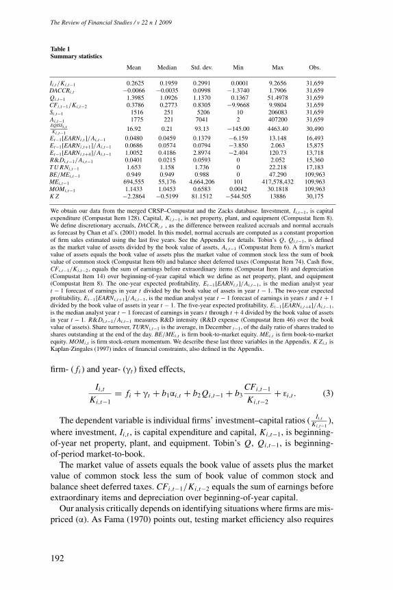
Table 1Summary statistics

Mean Median Std. dev. Min Max Obs.

Ii,t /Ki,t−1 0.2625 0.1959 0.2991 0.0001 9.2656 31,659DACCRi,t −0.0066 −0.0035 0.0998 −1.3740 1.7906 31,659Qi,t−1 1.3985 1.0926 1.1370 0.1367 51.4978 31,659CFi,t−1/Ki,t−2 0.3786 0.2773 0.8305 −9.9668 9.9804 31,659Si,t−1 1516 251 5206 10 206083 31,659Ai,t−1 1775 221 7041 2 407200 31,659EQISSi,tKi,t−1

16.92 0.21 93.13 −145.00 4463.40 30,490

Et−1[EARNi,t ]/Ai,t−1 0.0480 0.0459 0.1379 −6.159 13.148 16,493Et−1[EARNi,t+1]/Ai,t−1 0.0686 0.0574 0.0794 −3.850 2.063 15,875Et−1[EARNi,t+4]/Ai,t−1 1.0052 0.4186 2.8974 −2.404 120.73 13,718R&Di,t−1/Ai,t−1 0.0401 0.0215 0.0593 0 2.052 15,360T U RNi,t−1 1.653 1.158 1.736 0 22.218 17,183BE/MEi,t−1 0.949 0.949 0.988 0 47.290 109,963MEi,t−1 694,555 55,176 4,664,206 101 417,578,432 109,963MOMi,t−1 1.1433 1.0453 0.6583 0.0042 30.1818 109,963K Z −2.2864 −0.5199 81.1512 −544.505 13886 30,175

We obtain our data from the merged CRSP–Compustat and the Zacks database. Investment, Ii,t−1, is capitalexpenditure (Compustat Item 128). Capital, Ki,t−1, is net property, plant, and equipment (Compustat Item 8).We define discretionary accruals, DACCRi,t , as the difference between realized accruals and normal accrualsas forecast by Chan et al’s. (2001) model. In this model, normal accruals are computed as a constant proportionof firm sales estimated using the last five years. See the Appendix for details. Tobin’s Q, Qi,t−1, is definedas the market value of assets divided by the book value of assets, Ai,t−1 (Compustat Item 6). A firm’s marketvalue of assets equals the book value of assets plus the market value of common stock less the sum of bookvalue of common stock (Compustat Item 60) and balance sheet deferred taxes (Compustat Item 74). Cash flow,CFi,t−1/Ki,t−2, equals the sum of earnings before extraordinary items (Compustat Item 18) and depreciation(Compustat Item 14) over beginning-of-year capital which we define as net property, plant, and equipment(Compustat Item 8). The one-year expected profitability, Et−1[EARNi,t ]/Ai,t−1, is the median analyst yeart − 1 forecast of earnings in year t divided by the book value of assets in year t − 1. The two-year expectedprofitability, Et−1[EARNi,t+1]/Ai,t−1, is the median analyst year t − 1 forecast of earnings in years t and t + 1divided by the book value of assets in year t − 1. The five-year expected profitability, Et−1[EARNi,t+4]/Ai,t−1,is the median analyst year t − 1 forecast of earnings in years t through t + 4 divided by the book value of assetsin year t − 1. R&Di,t−1/Ai,t−1 measures R&D intensity (R&D expense (Compustat Item 46) over the bookvalue of assets). Share turnover, TURNi,t−1 is the average, in December t−1, of the daily ratio of shares traded toshares outstanding at the end of the day. BE/MEi,t is firm book-to-market equity. MEi,t is firm book-to-marketequity. MOMi,t is firm stock-return momentum. We describe these last three variables in the Appendix. K Zi,t isKaplan-Zingales (1997) index of financial constraints, also defined in the Appendix.

firm- ( fi ) and year- (γt ) fixed effects,

Ii,t

Ki,t−1= fi + γt + b1αi,t + b2 Qi,t−1 + b3

CFi,t−1

Ki,t−2+ εi,t . (3)

The dependent variable is individual firms’ investment–capital ratios ( Ii,t

Ki,t−1),

where investment, Ii,t , is capital expenditure and capital, Ki,t−1, is beginning-of-year net property, plant, and equipment. Tobin’s Q, Qi,t−1, is beginning-of-period market-to-book.

The market value of assets equals the book value of assets plus the marketvalue of common stock less the sum of book value of common stock andbalance sheet deferred taxes. CFi,t−1/Ki,t−2 equals the sum of earnings beforeextraordinary items and depreciation over beginning-of-year capital.

Our analysis critically depends on identifying situations where firms are mis-priced (α). As Fama (1970) points out, testing market efficiency also requires

192


a model of market equilibrium. Thus, any evidence linking investment to mis-pricing can never be conclusive as that mispricing can also be interpreted ascompensation for exposure to risk. Therefore, although we use discretionary ac-cruals, a variable that is difficult to link to risk, we note that our evidence couldbe interpreted as rational under some unspecified model of market equilibrium.

Our proxy for mispricing exploits firms’ use of accrual accounting. Accrualsrepresent the difference between a firm’s accounting earnings and its underlyingcash flow. For example, large positive accruals indicate that earnings are muchhigher than the cash flow generated by the firm.

Several papers show a strong correlation between discretionary accruals andsubsequent stock returns, suggesting that firms with high discretionary accrualsare overpriced relative to otherwise similar firms. For example, Sloan (1996)finds that those firms with relatively high (low) levels of abnormal accruals ex-perience negative (positive) future abnormal stock returns concentrated aroundfuture earning announcements. Teoh, Welch, and Wong (1998a,b) find that IPOand SEO firms who have the highest discretionary accruals have the lowest ab-normal returns post equity issue. More recently, Chan et al. (2001) investigatethe relation between discretionary accruals and stock returns. Confirming pre-vious results, they also find that firms with high (low) discretionary accrualsdo poorly (well) over the subsequent year. Most of the abnormal performanceis concentrated in the firms with very high discretionary accruals.6

We use past evidence on the correlation between discretionary accruals andstock returns to justify the use of discretionary accruals as our mispricing proxy.We measure accruals (ACCRi,t ) by

ACCR(i,t) = �NCCA − �CL − DEP, (4)

where �NCCA is the change in noncash current assets, �CL is the changein current liabilities minus the change in debt included in current liabilitiesand minus the change in income taxes payable, and DEP is depreciation andamortization.

The differences between earnings and cash flow arise because of accountingconventions as to when, and to what extent, firms recognize revenues and costs.Within those conventions, managers have discretion over accruals adjustmentsand may use them to manage earnings. For example, a manager can modifyaccruals by delaying recognition of expenses after advancing cash to suppli-ers, by advancing recognition of revenues with credit sales, by deceleratingdepreciation, or by assuming a low provision for bad debt.

To capture the discretionary component of discretionary accruals, we followChan et al. (2001) such that

DACCRi,t = ACCRi,t − NORMALACCRi,t , (5)

6 These results are puzzling because, in principle, if investors can detect earnings manipulation, higher accrualsshould not affect the stock price. However, a large body of evidence indicates that investors seem to simply focuson earnings (see Hand, 1990; and Maines and Hand, 1996).

193


NORMALACCRi,t =∑5

k=1 ACCRi,t−k∑5k=1 SALESi,t−k

SALESi,t , (6)

where we scale accruals by total assets and model NORMALACCRi,t as aconstant proportion of firm sales. In other words, to capture the discretionarycomponent of accruals, we assume that the necessary accruals adjustments arefirm-specific.7 For example, asset-intensive firms typically have relatively highdepreciation.

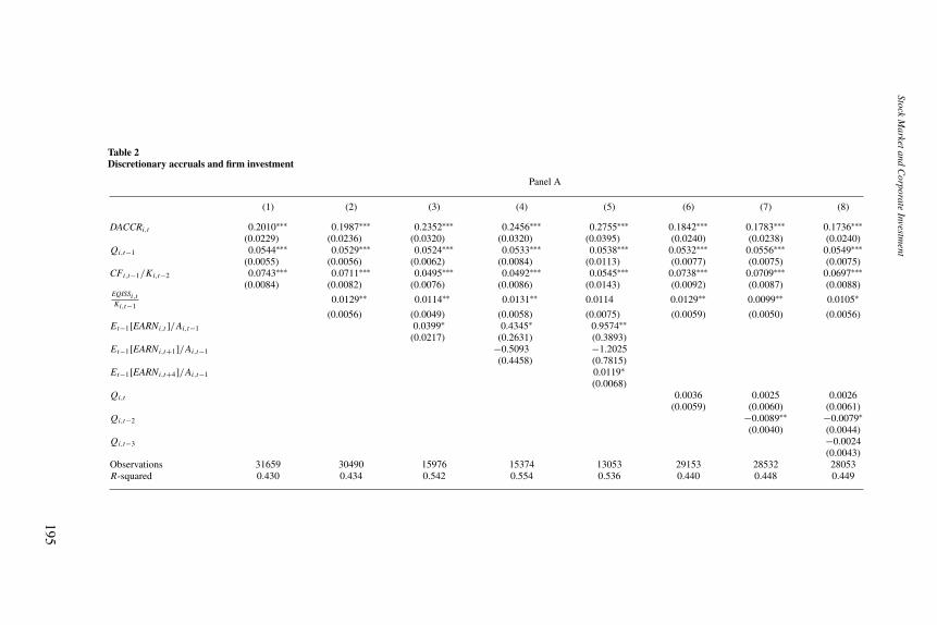
In Table 2, Panel A, column (1) displays the results of regression (3). Whenwe control for investment opportunities and cash flow, we find that firms withhigh discretionary accruals invest more. The coefficient of investment on dis-cretionary accruals measures 0.201 with an associated t-statistic of 8.78. Firmswith abnormally soft earnings invest more than the standard model would indi-cate. This effect is economically important. A one-standard-deviation changein a typical firm’s level of discretionary accruals is associated with roughlya 2% change in that firm’s investment as a percentage of capital, which cor-responds to 7% of the sample mean. Our results are consistent with a recentpaper by Bergstresser, Desai, and Rauh (2004) that shows that a specific typeof earnings manipulation based on the assumed rate of return on pension assetsfor companies with defined benefit pension plans is correlated with investmentdecisions.

Note that Abel and Blanchard (1986) suggest that mispricing may smear theinformation in Q concerning investment opportunities. This possibility actuallyworks against us finding any independent effect of discretionary accruals. IfQ is correlated with mispricing, then the coefficient of discretionary accrualsunderestimates the effect of mispricing on investment.

One way to interpret our results is that overpriced equity allows firms toissue equity and finance investment. Baker, Stein, and Wurgler (2003) showthat mispricing affects investment decisions through an equity channel. Firmsthat are overpriced issue more equity (Baker and Wurgler, 2000, 2002). If thefirm is cash constrained and is not investing optimally before issuing equity,then more equity issuance translates into more investment.

As noted above, we want to test whether there is an additional channel thatlinks equity mispricing to investment. We want to find out if managers cater

7 We have also estimated (Polk and Sapienza, 2004) the discretionary component of accruals using the cross-sectional adaptation developed in Teoh, Welch, and Wong (1998a,b) of the modified Jones’ (1991) model.Specifically, we estimated expected current accruals for each firm in a given year from a cross-sectional regressionin that year of current accruals on the change in sales using an estimation sample of all two-digit SIC codepeers. All our results are substantially the same when we use this alternative measure. Hribar and Collins(2002) argue that the Jones’ method is potentially flawed as it calculates accruals indirectly using balancesheet information rather than directly using income statement information. In particular, they point out thatthe presumed equivalence between the former and the latter breaks down when nonoperating events, such asreclassifications, acquisitions, divestitures, accounting changes, and foreign currency translations occur. Hribarand Collins show that these “non-articulating” events generate nontrivial measurement error in calculations ofdiscretionary accruals. However, our results still hold even when we restrict the analysis to a subsample of firmsthat do not have such nonarticulation events or when we use income statement accruals in a post-1987 sample,where the necessary income-statement accruals information is available.

194

StockM

arketandC

orporateInvestm

ent

Table 2Discretionary accruals and firm investment

Panel A

(1) (2) (3) (4) (5) (6) (7) (8)

DACCRi,t 0.2010∗∗∗ 0.1987∗∗∗ 0.2352∗∗∗ 0.2456∗∗∗ 0.2755∗∗∗ 0.1842∗∗∗ 0.1783∗∗∗ 0.1736∗∗∗(0.0229) (0.0236) (0.0320) (0.0320) (0.0395) (0.0240) (0.0238) (0.0240)

Qi,t−1 0.0544∗∗∗ 0.0529∗∗∗ 0.0524∗∗∗ 0.0533∗∗∗ 0.0538∗∗∗ 0.0532∗∗∗ 0.0556∗∗∗ 0.0549∗∗∗(0.0055) (0.0056) (0.0062) (0.0084) (0.0113) (0.0077) (0.0075) (0.0075)

CFi,t−1/Ki,t−2 0.0743∗∗∗ 0.0711∗∗∗ 0.0495∗∗∗ 0.0492∗∗∗ 0.0545∗∗∗ 0.0738∗∗∗ 0.0709∗∗∗ 0.0697∗∗∗(0.0084) (0.0082) (0.0076) (0.0086) (0.0143) (0.0092) (0.0087) (0.0088)

EQISSi,tKi,t−1

0.0129∗∗ 0.0114∗∗ 0.0131∗∗ 0.0114 0.0129∗∗ 0.0099∗∗ 0.0105∗

(0.0056) (0.0049) (0.0058) (0.0075) (0.0059) (0.0050) (0.0056)Et−1[EARNi,t ]/Ai,t−1 0.0399∗ 0.4345∗ 0.9574∗∗

(0.0217) (0.2631) (0.3893)Et−1[EARNi,t+1]/Ai,t−1 −0.5093 −1.2025

(0.4458) (0.7815)Et−1[EARNi,t+4]/Ai,t−1 0.0119∗

(0.0068)Qi,t 0.0036 0.0025 0.0026

(0.0059) (0.0060) (0.0061)Qi,t−2 −0.0089∗∗ −0.0079∗

(0.0040) (0.0044)Qi,t−3 −0.0024

(0.0043)Observations 31659 30490 15976 15374 13053 29153 28532 28053R-squared 0.430 0.434 0.542 0.554 0.536 0.440 0.448 0.449

195

The

Review

ofFinancialStudies

/v22

n1

2009

Table 2Continued

Panel B

(1) (2) (3) (4) (5) (6) (7)

DACCRi,t 0.1471∗∗∗ 0.1798∗∗ 0.1359∗∗ 0.0982 0.1387∗∗∗ 0.1406∗∗∗ 0.1390∗∗∗(0.0340) (0.0715) (0.0538) (0.0651) (0.0337) (0.0342) (0.0349)

Qi,t−1 0.0441∗∗∗ 0.0373∗∗∗ 0.0382∗∗∗ 0.0159 0.0387∗∗∗ 0.0410∗∗∗ 0.0421∗∗∗(0.0108) (0.0116) (0.0123) (0.0111) (0.0126) (0.0121) (0.0115)

CFi,t−1/Ki,t−2 0.0744∗∗∗ 0.0796∗∗ 0.0836∗∗ 0.1073∗ 0.0702∗∗∗ 0.0712∗∗∗ 0.0649∗∗∗(0.0140) (0.0327) (0.0360) (0.0626) (0.0141) (0.0145) (0.0135)

Et−1[EARNi,t ]/Ai,t−1 0.0655∗∗ −0.0475 0.1529(0.0301) (0.1359) (0.3496)

Et−1[EARNi,t+1]/Ai,t−1 0.1404 0.4248(0.2018) (0.2819)

Et−1[EARNi,t+4]/Ai,t−1 0.0130(0.0117)

Qi,t 0.0068 0.0073 0.0062(0.0093) (0.0098) (0.0096)

Qi,t−2 −0.0131∗∗ −0.0077(0.0065) (0.0065)

Qi,t−3 −0.0066(0.0079)

Observations 10433 0 3528 2825 10132 9854 9600R-squared 0.426 0.569 0.605 0.630 0.433 0.447 0.466

The dependent variable is the proportion of investment over beginning-of-year capital. For a description of all the other variables, see the legend of Table 1. Panel A shows the results forthe entire sample. All columns report coefficients and standard errors from OLS regressions. In Panel B, we repeat the same specification, but now we exclude companies that have positiveequity issuance (Compustat Item 108). All regressions include firm- and year-fixed effects. The standard errors reported in parentheses are corrected for clustering of the residual at thefirm level. Coefficients starred with one, two, and three asterisks are statistically significant at the 10%, 5%, and 1% levels, respectively.

196


to investor demand by investing more when investors overprice the stock. Theinvestment catering channel works independently from the decision to issueequity, because managers can temporarily boost the stock price by investingmore.

To test whether our results are consistent with the catering channel, in Table 2,Panel A, column (2), and all in subsequent similar regressions, we control forcash from the sale of common and preferred stocks (Compustat Item 108) scaledby Ki,t−1 (beginning-of-year net property, plant, and equipment), EQISSi,t

Ki,t−1.

We find that a one-standard-deviation change in equity issuance positivelyaffects investment by a 1.2% change in that firm’s investment as a percentageof capital. This finding is consistent with Baker, Stein, and Wurgler (2003).More important for our hypothesis, the discretionary accruals coefficient re-mains essentially the same as before, confirming that the catering channel hasan independent effect: One-standard-deviation change in the firm’s level ofdiscretionary accruals is associated with a 2% change in firm investment overcapital, which corresponds to 7% of the sample mean.

There are several potential problems in our baseline regression that mightundermine the interpretation of the results. The most obvious problem arisesfrom the fact that the disappointing performance of our measure of Q, even ifit is consistent with the results in other studies, suggests that this measure maybe a poor proxy for true marginal Q.8

If our mispricing variable is a good indicator of unobserved investmentopportunities, then the existence of measurement error in Tobin’s Q is a par-ticularly serious problem in our analysis. For example, we could argue thatfirms with high discretionary accruals may have very profitable growth optionsthat their average Q only partially reflects. These firms should invest more.Fortunately, the evidence in other studies suggests exactly the opposite: firmswith soft earnings are firms with poor growth opportunities. Teoh, Welch, andWong (1998b) document that firms with high discretionary accruals tend to beseasoned equity issuers with relatively low postissue net income. Chan et al.(2001) show that, in general, firms with high discretionary accruals subse-quently have a marked deterioration in their cash flows. Based on these findings,our measure of firm’s mispricing is particularly appropriate in this context: it ishard to argue that the average Q for this type of firm systematically understatesmarginal Q.

8 Several papers have addressed this issue and found different results. For example, Abel and Blanchard (1986)construct aggregate marginal Q and find little support for the view that the low explanatory power of averageQ is because it is a poor proxy for marginal Q. Similarly, Gilchrist and Himmelberg (1995) exploit Abel andBlanchard’s technique at the level of the individual firm. Though their marginal Q series seems to perform betterthan Tobin’s Q, their qualitative results are not very different from the previous literature. Of course, their resultscritically depend on the quality of the alternative measure used. In a recent paper, Erickson and Whited (2000)point out that the various measures generally used in the literature all have an errors-in-variables problems andsuggest an alternative solution. Erickson and Whited use a measurement-error-consistent generalized method ofmoments estimator that relies on information in higher moments of Q. With this estimator, they find that theaccepted results in the previous literature (low explanatory power of Tobin’s Q and high explanatory power ofcash flow) disappear.

197


Even though current empirical studies suggest that abnormal noncash earn-ings are not positively correlated with investment opportunities, we still useseveral strategies from these studies on investment and Q to address mea-surement error problems in our proxy for investment opportunities. First, weinclude analysts’ consensus estimates of future earnings in our baseline regres-sion. If analysts’ forecasts are a good proxy for expected future profitability,this variable may be a good proxy for marginal Q. If we control for average Q,then higher marginal Q should be positively correlated with higher expectedfuture profitability.

In columns (2) through (4) of Table 2, Panel A, we add the ratio of con-sensus analyst forecast of cumulative firm profitability over assets one, two,and five years out to our baseline specification. The one-year earnings forecasthas a positive effect on firms’ investment decisions. The effect is small, butstatistically significant at the 5% level. A one-standard-deviation change in theone-year earning forecast is associated with roughly a 0.5% change in thatfirm’s investment-to-capital ratio. This result suggests that this nonfinancialmeasure of future profitability has some information, even when we control forTobin’s Q. However, the coefficient on discretionary accruals actually increasesfrom 0.1987 to 0.2352.

In column (4) of Table 2, Panel A, we add both one- and two-year prof-itability estimates to our baseline regression. Discretionary accruals continueto be significant. In column (5), we include one-, two-, and five-year prof-itability forecasts. Discretionary accruals remain economically and statisticallysignificant.9

We also follow Abel and Eberly (2002) by using the long-term consensusearnings forecast as an instrument for Q. This instrument could be problematicbecause first, it is likely to be correlated with the measurement error in Tobin’sQ; and second, as Bond and Cummins (2000) suggest, analyst forecasts mayhave an independent effect on investment. Nonetheless, when we estimate thatregression, we find that when we use instrumental variables estimation, thesignificance of the discretionary accruals coefficient (not reported) is similar toour previous results.

To deal with the measurement error problem, we implement the Ericksonand Whited (2000, 2002) method that exploits the information contained inhigher moments to generate measurement-error-consistent GMM estimators ofthe relation between the investment and Q, and, consistent with their resultsand with the claim that there is measurement error in Q, we find that using thisestimator increases the coefficient on Q by an order of magnitude.10 Thoughour sample is reduced to satisfy the identifying assumption of Erickson and

9 Although we might be initially surprised by the negative coefficient on Et−1[EARNi,t+1]/Ai,t−1, since earningsestimates are for cumulative earnings from t − 1 to t , the negative coefficient indicates that the consensusone-year earnings two years from now have a relatively smaller impact on investment than consensus one-yearearnings one year from now. In this light, the result seems reasonable.

10 We thank Toni Whited for providing the Gauss code implementing their estimator.

198


Whited (2000), the coefficient on discretionary accruals remains economicallyand statistically significant. (These results are available on request.)

Another potential problem with our baseline regression could arise becausewe measure average Q at the beginning of the year in which we measure thefirm’s investment, but perhaps the firm’s investment opportunities change overthe year. As a result, our discretionary accruals measure might pick up thischange in investment opportunities. Therefore, in Table 2, Panel A, column(6), we add to the baseline specification, end-of-period Qi,t . Controlling forthe change in Q over the investment period has no effect on our results. Invest-ment opportunities measured by end-of-period Tobin’s Q are not statisticallysignificant and the estimated coefficient is 1/20 of that on Qi,t−1 in the baselineregression. Moreover, the estimated coefficient on discretionary accruals andthe statistical significance of that estimate do not change.

We wish to ensure that our controls for investment opportunities are adequateif there is a lag between the time when a firm has investment opportunities andwhen we measure the actual investment. Therefore, the next two specificationsinclude lags of Q in response. In Table 2, Panel A, column (7), we add Qt−2

to the specification in column (6). Although lagged investment opportunitiesexplain firm investment, discretionary accruals still have a positive and signifi-cant effect on firm investment. Column (8) adds Qt−3 to our specification. Thisvariable is not significant and our results do not change. We conclude that thetiming of our Tobin’s Q variable is not an issue.

We also examine the possibility that if discretionary accruals are correlatedwith a firm’s amount of financial slack, then our variable might be pickingup on the fact that financially constrained firms have less financial slack withwhich to invest. Firms with high discretionary accruals are those firms whoseearnings are not backed by cash flow: firms with high discretionary accrualsgenerally have little financial slack. However, we augment our baseline re-gression with both contemporaneous and two- and three-year lags of our cashflow variable, CFi,t−1/Ki,t−2, as well as with measures of the cash stock. Theresults (unreported) are robust to this modification. One possible reason thatfirms manipulate earnings is to meet bond covenants; our results are also robustto including leverage as an additional explanatory variable.

We want to verify that the relation between discretionary accruals andinvestment is not hardwired. For example, firms with multiyear investmentprojects may pay for investment in advance. When doing so, firms will bookfuture investment as a prepaid expense, a current asset. If so, current invest-ment and discretionary accruals (the prepaid expense) may exhibit a posi-tive correlation. Therefore, we reestimate the regression, now measuring nor-mal accruals by using only accounts receivable in the definition of accruals.In that regression (not reported), the coefficient associated with the discre-tionary component of accounts receivable remains economically and statis-tically significant. We conclude that this hardwired link is not driving ourresult.

199


In Table 2, Panel B provides additional investigation of the robustness ofour results. Instead of including equity issuance as a control, we reestimatethe regressions in Table 2, Panel A, by excluding all the companies that havepositive equity issuance (Compustat Item 108). We find that all of our resultscontinue to hold and are still generally statistically significant, even though thesample is now smaller by two-thirds. The effect of discretionary accruals oninvestment is still economically significant for firms that do not issue equity.A one-standard-deviation change in the level of discretionary accruals affectsinvestment over capital by 1.5%, which corresponds to 5% of the sample mean.

2.3 Cross-sectional testsOur model suggests that the greater the opacity of the firm and the shorter thetime horizon of the firm’s shareholders, the more likely managers are to caterinvestments.

In Table 3, we explore these cross-sectional implications of our model.We use firm R&D intensity as our proxy for firm transparency, based onthe assumption that the resolution of all valuation uncertainty, which wouldnecessarily eliminate any mispricing, takes longer for R&D projects than forother types of projects.

We first estimate our model for those firms that have data on R&D. We reportthese results in column (1). Column (2) reestimates our baseline regression forthose firms below the median value of R&D intensity. We note that we calculatemedians yearly in order to isolate pure cross-sectional differences across firms.Column (3) shows the results for the subsample of firms with R&D intensityabove the median. Consistent with our model, we find economically importantvariation across the two subsamples. Firms that engage in a lot of R&D investmore when they have a lot of discretionary accruals. The sensitivity of thesefirms’ investment to discretionary accruals, 0.3154, is almost two times as largeas the sensitivity of firms that we argue are relatively more transparent.

The theory of catering investment relies on the assumption that either theshareholders or the manager of the firm have short-term horizons (Stein, 1996).Thus, our finding that discretionary accruals affect firm investment should bestronger for firms with a higher fraction of short-term investors. We test thishypothesis by using firm share turnover as our proxy for the relative amount ofshort-term investors trading a firm’s stock. We measure turnover as the average,in Decembert−1, of the daily ratio of shares traded to shares outstanding at theend of the day, following Gaspar, Massa, and Matos (2005).

We first estimate our model for those firms that have data on turnover. Wereport these results in Table 3, column (4). Column (5) reestimates for each yearour baseline regression for those firms with turnover below the yearly median,while column (6) reports the regression results for above-the-median firms.We find that the coefficient on discretionary accruals for high-turnover firms is0.1726, roughly 50% higher than the corresponding coefficient for firms withlow turnover.

200

StockM

arketandC

orporateInvestm

ent

Table 3Discretionary accruals and firm investment: Cross-sectional analysis

Panel A

(1) (2) (3) (4) (5) (6) (7) (8) (9) (10)

DACCRi,t 0.2455∗∗∗ 0.1542∗∗∗ 0.3052∗∗∗ 0.1537∗∗∗ 0.1154∗∗ 0.1726∗∗∗ 0.1584∗∗∗ 0.1572∗∗∗ 0.2927∗∗∗ 0.3433∗∗∗(0.0345) (0.0405) (0.0533) (0.0283) (0.0501) (0.0346) (0.0290) (0.0234) (0.0531) (0.0758)

Qi,t−1 0.0495∗∗∗ 0.0687∗∗∗ 0.0461∗∗∗ 0.0454∗∗∗ 0.0384∗∗∗ 0.0547∗∗∗ 0.0527∗∗∗ 0.0529∗∗∗ 0.0532∗∗∗ 0.0483∗∗∗(0.0062) (0.0146) (0.0072) (0.0079) (0.0077) (0.0095) (0.0056) (0.0055) (0.0079) (0.0100)

CFi,t−1/Ki,t−2 0.0694∗∗∗ 0.1103∗∗∗ 0.0597∗∗∗ 0.1042∗∗∗ 0.1153∗∗∗ 0.0918∗∗∗ 0.0712∗∗∗ 0.0719∗∗∗ 0.0373∗∗∗ 0.0221∗∗(0.0100) (0.0255) (0.0098) (0.0172) (0.0200) (0.0224) (0.0082) (0.0082) (0.0094) (0.0092)

EQISSi,tKi,t−1

0.0241∗∗∗ 0.0278 0.0198∗∗∗ −0.0047 −0.0091 0.0060 0.0129∗∗ 0.0129∗∗ 0.0162∗∗∗ 0.0145

(0.0074) (0.0178) (0.0066) (0.0071) (0.0069) (0.0107) (0.0056) (0.0055) (0.0061) (0.0118)HIGHDACCRi,t 0.0162∗∗∗

(0.0058)highseo 0.1684∗∗

(0.0659)Observations 14838 7684 7154 16380 6796 9584 30490 30490 7776 3956R-squared 0.484 0.433 0.535 0.412 0.525 0.447 0.434 0.434 0.510 0.595

201

The

Review

ofFinancialStudies

/v22

n1

2009

Table 3Continued

Panel B

(1) (2) (3) (4) (5) (6) (7) (8) (9)

DACCRi,t 0.1599∗∗∗ 0.0941∗ 0.2894∗∗ 0.0877∗ 0.0279 0.1593∗∗∗ 0.1211∗∗∗ 0.3917∗∗ 0.2409(0.0537) (0.0540) (0.1219) (0.0477) (0.0906) (0.0573) (0.0392) (0.1527) (0.2038)

Qi,t−1 0.0250∗∗ 0.0323∗∗ 0.0117 0.0473∗∗∗ 0.0399∗∗∗ 0.0593∗∗ 0.0442∗∗∗ 0.0479∗∗ 0.1064∗∗(0.0100) (0.0140) (0.0158) (0.0151) (0.0138) (0.0237) (0.0108) (0.0203) (0.0493)

CFi,t−1/Ki,t−2 0.0828∗∗∗ 0.0889∗∗∗ 0.0845∗∗∗ 0.0873∗∗∗ 0.1230∗∗∗ 0.0473∗∗ 0.0744∗∗∗ 0.0480 0.0244(0.0147) (0.0219) (0.0218) (0.0190) (0.0350) (0.0196) (0.0140) (0.0724) (0.0676)

HIGHDACCRi,t 0.0114(0.0083)

Observations 4658 3061 1597 5959 3044 2915 10433 1841 821R-squared 0.430 0.445 0.447 0.433 0.468 0.615 0.427 0.569 0.650

The dependent variable is the proportion of investment over beginning-of-year capital. High discretionary accruals, HIGHDACCRi,t−1, is a dummy equal to 1 if the firm has discretionaryaccruals in the top 20th percentile, and 0 otherwise. High equity issuance activity, HIGHEQISSUEi,t−1, is a dummy equal to 1 if the firm had equity issuance in the top 25th percentile inthe previous five years, and 0 otherwise. For a description of all the other variables, see the legend of Table 1. Panel A shows the results for the entire sample. All columns report coefficientsand standard errors from OLS regressions. In Panel B, we repeat the same specification, but now we exclude companies that have positive equity issuance (Compustat Item 108). Column(1) shows results for the firms that have valid R&D intensity data. Column (2) shows results for the firms that have below-median R&D intensity. Column (3) shows results for those firmsthat have above-median R&D intensity. Column (4) shows results for those firms that have valid firm share turnover data. Column (5) shows results for those firms that have below-medianfirm share turnover. Column (6) shows results for those firms that have above-median firm share turnover. We calculate medians on a year-by-year basis. Columns (7) and (8) show resultsfor the whole sample. Column (9) shows results for the firm-years in the subperiod, 1995–2000. Column (10) shows results for the firm-years in the subperiod, 1998–2000. Columns (1)–(7)in Panel B correspond to columns (1)–(7) in Panel A. Columns (8)–(9) in Panel B correspond to columns (9)–(10) in Panel A. All regressions include firm- and year-fixed effects. Thestandard errors reported in parentheses are corrected for clustering of the residual at the firm level. Coefficients starred with one, two, and three asterisks are statistically significant at the10%, 5%, and 1% levels, respectively.

202


Previous literature provides additional tests of our hypothesis based on sub-sample and cross-sectional evidence. We now explore these implications. Chanet al. (2001); and D’Avolio, Gildor, and Shleifer (2002) point out that the abilityof discretionary accruals to predict negative stock returns is concentrated in thetop 20% of firms ranked on accruals.

In Table 3, Panel A, column (7), we add a dummy, HIGHDACCRi,t , to ourbaseline discretionary accruals specification. The dummy takes the value of 1if the firm is in the top 20% of firms based on discretionary accruals, and 0otherwise. This dummy is significant at the 5% level of significance.

Teoh, Welch, and Wong (1998a) show that firms issuing equity who havethe highest discretionary earnings have the lowest abnormal returns. In Table3, Panel A, column (8), we interact our discretionary accruals variable with adummy, HIGHSEOi,t , that takes the value 1 if the firm is in the top 25% ofequity issuance, as determined by Daniel and Titman’s (2006) composite equityissuance variable.11 The coefficient is positive and has a t-statistic of 2.56.

D’Avolio, Gildor, and Shleifer (2002) argue that in recent years, the marginalinvestor may have become less sophisticated, providing more incentives todistort earnings. In particular, they show that the mean discretionary accrualsfor the top decile has been increasing over the past 20 years, more than doublingsince 1974. Mean discretionary earnings for the top decile was close to 30% in1999.

In Table 3, Panel A, column (9), we reestimate our baseline specificationfor the firm-years in the subperiod 1995–2000. The estimated coefficient ondiscretionary accruals is roughly two-thirds bigger, moving from 0.1987 to0.2927. Although we are left with only a quarter of the number of observations,the estimate is statistically significant at the 1% level. In column (10), wefurther restrict the sample to only those firm-years in the subperiod 1998–2000. Consistent with the hypothesis that manipulating earnings has becomemore effective, we find that the coefficient on discretionary accruals is morethan 70% higher than in the baseline regression.

Panel B of Table 3 repeats our cross-sectional and subperiod tests of thecatering hypothesis by restricting the sample to firms that do not have netpositive cash flow from equity issuance. We find that our conclusions fromPanel A do not change, even though we sometimes lose statistical power dueto the reduction in size of the sample.

2.4 Efficient or inefficient investment?So far, we have found a consistently strong positive correlation between ourmeasures of mispricing and investment. According to the model, the positivecorrelation is due to the fact that overpriced firms take investment projects that

11 Following Daniel and Titman (2006), we construct a measure of a firm’s equity issuance/repurchase activity,SEOi,t , over a five-year period. We define SEOi,t as the log of the inverse of the percentage ownership in thefirm one would have at time t , given a 1firm at time t − 5, assuming full reinvestment of all cash flows.

203


have negative net present values. Similarly, underpriced firms forego invest-ment projects with positive net present value. While the empirical results areconsistent with inefficient allocation of resources in equilibrium, there are otherpotential explanations.

First, it is possible that firms with good investment opportunities manageearnings (i.e., generate high discretionary accruals) to manipulate their stockprice, facilitating investment. The investment allocation in this case is efficientand temporary mispricing helps financially constrained firms make investmentsthat they otherwise would not be able to make. This interpretation, thoughplausible, is not consistent with previous findings (e.g., Chan et al., 2001) thatshow that firms with abnormally soft earnings actually have relatively pooroperating performance in subsequent years. Another potential explanation forour results is outlined in Dow and Gorton (1997). In that model, when themarket has information that managers do not have, it is efficient for managersto make investment decisions taking into account stock prices. However, sincediscretionary accruals are set by the manager, this story seems unlikely toexplain the relation between discretionary accruals and investment. Finally,our mispricing proxies may instead represent rational heterogeneity in discountrates. In this alternative explanation, firms with high discretionary accruals havelow discount rates.

To distinguish between these alternative explanations, we measure the rela-tion between investment and future stock returns. In our model, because firmbusiness investment is linked to the market’s misvaluation of the firm’s equity,there is a negative relation between investment and subsequent risk-adjustedreturns.

We estimate cross-sectional regressions of monthly stock returns on invest-ment, Tobin’s Q, and a control for cash-flow sensitivity,12

Ri,t = at + b1,t lnIi,t−1

Ki,t−2+ b2,t ln Qi,t−1 + b3,t

CFi,t−1

Ki,t−2, (7)

where we measure returns in percentage units. The regression identifies cross-sectional variation in returns, which is correlated with investment, and controlsfor investment opportunities and financial slack. Thus, the regression ties returnpredictability to firm investment behavior.

Unlike the previous sample in which we use only December-year-end firms,here we use all available data as long as there is a five-month lag between themonth in which we are predicting returns and the fiscal year-end. We do thisto ensure that the regression represents a valid trading rule. As in the previoussample, we eliminate firms with negative investment and/or otherwise extremeaccounting ratios.

12 We are not the first looking at the relation between investment and returns. Titman, Wei, and Xie (2004) showthat firms that spend more on capital investment relatively to their sales or total assets subsequently have negativebenchmark-adjusted returns. See also Baker, Stein, and Wurgler (2003).

204


As in Fama and MacBeth (1973), we average the time series of bt ’s and reportboth the mean and the standard error of the mean estimate. Table 4, column(1), shows the result of estimating Equation (7). The coefficient on investmentis −0.1579 with an associated t-statistic of 3.96. Consistent with our model,firms that overinvest (underinvest) on average have returns that are low (high).

We note that identification might be easier in this framework. In our pre-vious investment regressions, controls for marginal profitability were criticalfor isolating variation in investment linked to mispricing. In theory, in thesereturn regressions, we need only control for risk. Table 4, column (2), includesthree firm characteristics that are associated with cross-sectional differences inaverage returns that may or may not be associated with risk: firm size (marketcapitalization), firm book-to-market equity, and firm momentum. These char-acteristics are known anomalies that we want to control for. Our results confirmthe results of previous studies: book-to-market equity and firm momentum pre-dict returns with a positive coefficient, while size has a negative coefficient.13

More importantly, these controls do not subsume the investment effect, sincethe relevant coefficient drops less than two basis points and remains quite sta-tistically significant. We also include the control variable for equity issuance,EQISSi,t−1

Ki,t−2. Consistent with previous research, we find that firms issuing equity

subsequently underperform.Our model predicts that this return predictability we document should be

stronger for firms facing a greater degree of information asymmetry and/or hav-ing investors with shorter horizons. In Table 4, we test these predictions by esti-mating the degree of return predictability linked to abnormal investment for highR&D-intensity and high share-turnover firms. In column (3), we reestimate therelation between investment and subsequent stock returns for those firms withavailable R&D data each year. In column (4), we reestimate the relation by in-cluding an interaction variable between investment and an above-median R&Ddummy variable. The regression shows that the abnormal-investment effect inthe cross-section of average returns is mainly in high R&D firms. The t-statisticon this interaction term is 3.35. The ability of investment to predict cross-sectional differences in returns is not statistically significant for low R&D firms.

In column (5) of Table 4, we reestimate the full regression for those firmswith available share turnover data, and in column (6) we reestimate the rela-tion by using an interaction term between above-median share turnover andinvestment. For the full sample of firms with available turnover data, the abnor-mal investment effect is less strong. In fact, the coefficient is not statisticallysignificant.

As noted earlier, our model predicts that the effect will be stronger for thosefirms with above-median turnover. We find results consistent with our model:

13 Though one might initially think that using Q and BE/ME in the same regression might be problematic, it turnsout that the two variables are not so highly correlated as to cause multicollinearity problems. Nevertheless, wehave checked to make sure that our results are not sensitive to the decision to include both variables in theregression.

205

The

Review

ofFinancialStudies

/v22

n1

2009

Table 4Investment and future stock returns

Panel A

(1) (2) (3) (4) (5) (6) (7) (8) (9)

Intercept 1.359∗∗∗ 3.632∗∗∗ 4.252∗∗∗ 4.088∗∗∗ 2.308∗∗∗ 2.375∗∗∗ 3.636∗∗∗ 3.693∗∗∗ 3.608∗∗∗(0.354) (0.788) (0.895) (0.868) (0.796) (0.815) (0.790) (0.782) (0.772)

lnIi,t−1/Ki,t−2 −0.156∗∗∗ −0.143∗∗∗ −0.123∗∗∗ 0.005 −0.074 −0.029 −0.145∗∗∗ −0.216∗∗∗ −0.092∗∗(0.041) (0.036) (0.052) (0.075) (0.049) (0.061) (0.037) (0.043) (0.041)

lnIi,t−1/K ∗i,t−2HIGHRD −0.285∗∗∗

(0.085)lnIi,t−1/K ∗

i,t−2HIGHTURN −0.115∗∗(0.052)

lnIi,t−1/K ∗i,t−2HIGHKZ 0.108∗∗∗

(0.031)lnQi,t−1 −0.408∗∗∗ 0.280∗∗ 0.269∗∗ 0.213∗ 0.043 0.069 0.293∗∗ 0.273∗∗ 0.148

(0.126) (0.124) (0.133) (0.129) (0.171) (0.170) (0.127) (0.125) (0.132)lnCFi,t−1/Ki,t−2 0.012 −0.008 0.021 0.030 0.007 0.011 −0.018 −0.021 −0.002

(0.038) (0.030) (0.038) (0.037) (0.046) (0.046) (0.033) (0.033) (0.040)EQISSi,t−1/Ki,t−2 −0.422∗∗ −0.472∗∗∗ −0.727∗∗∗ −0.744∗∗∗ −0.200 −0.253 −0.446∗∗ −0.453∗∗ −0.386

(0.201) (0.195) (0.315) (0.314) (0.247) (0.244) (0.204) (0.198) (0.311)lnMEi,t−1 −0.209∗∗∗ −0.241∗∗∗ −0.222∗∗∗ −0.100∗ −0.106∗ −0.210∗∗∗ −0.215∗∗∗ −0.197∗∗∗

(0.055) (0.061) (0.058) (0.051) (0.052) (0.055) (0.054) (0.054)lnBE/MEi,t−1 0.332∗∗∗ 0.392∗∗∗ 0.417∗∗∗ 0.177 0.194∗ 0.329∗∗∗ 0.323∗∗∗ 0.192∗∗

(0.078) (0.095) (0.093) (0.108) (0.106) (0.079) (0.080) (0.088)lnMOMi,t−1 0.672∗∗∗ 0.475∗∗ 0.434∗∗ 0.908∗∗∗ 0.900∗∗∗ 0.686∗∗∗ 0.678∗∗∗ 0.690∗∗∗

(0.198) (0.216) (0.213) (0.227) (0.221) (0.199) (0.198) (0.206)DACCRi,t−1 −0.599∗∗

(0.268)Observations 456 456 456 456 444 444 456 456 336

206

StockM

arketandC

orporateInvestm

ent

Table 4Continued

Panel B

(1) (2) (3) (4) (5) (6) (7) (8) (9)

Intercept 1.517∗∗∗ 3.980∗∗∗ 4.504∗∗∗ 4.405∗∗∗ 2.315∗∗∗ 2.482∗∗∗ 3.986∗∗∗ 4.011∗∗∗ 3.645∗∗∗(0.336) (0.766) (0.940) (0.904) (0.828) (0.852) (0.771) (0.760) (0.759)

lnIi,t−1/Ki,t−2 −0.136∗∗∗ −0.141∗∗∗ −0.145∗ −0.089 −0.143∗∗∗ −0.082 −0.135∗∗∗ −0.172∗∗∗ −0.142∗∗∗(0.041) (0.040) (0.078) (0.079) (0.059) (0.065) (0.040) (0.047) (0.047)

lnIi,t−1/K ∗i,t−2HIGHRD −0.150∗

(0.088)lnIi,t−1/K ∗

i,t−2HIGHTURN −0.154∗∗∗(0.059)

lnIi,t−1/K ∗i,t−2HIGHKZ 0.051

(0.040)lnQi,t−1 −0.409∗∗∗ 0.370∗∗ 0.308 0.293 0.402 0.417 0.345∗ 0.315∗ 0.125

(0.125) (0.177) (0.254) (0.255) (0.272) (0.270) (0.183) (0.182) (0.199)lnCFi,t−1/Ki,t−2 −0.017 −0.011 0.015 0.013 0.016 0.018 −0.062 −0.059 0.111∗

(0.046) (0.040) (0.071) (0.071) (0.066) (0.066) (0.048) (0.047) (0.061)lnMEi,t−1 −0.244∗∗∗ −0.272∗∗∗ −0.262∗∗∗ −0.104∗ −0.118∗∗ −0.241∗∗∗ −0.245∗∗∗ −0.212∗∗∗

(0.058) (0.068) (0.065) (0.057) (0.058) (0.058) (0.057) (0.057)lnBE/MEi,t−1 0.322∗∗∗ 0.364∗∗∗ 0.388∗∗∗ 0.351∗∗∗ 0.367∗∗∗ 0.301∗∗∗ 0.287∗∗∗ 0.204∗

(0.098) (0.145) (0.145) (0.142) (0.141) (0.100) (0.100) (0.113)lnMOMi,t−1 0.309 −0.025 −0.046 0.493∗ 0.462∗ 0.306 0.299 0.335

(0.196) (0.230) (0.230) (0.257) (0.253) (0.198) (0.196) (0.211)DACCRi,t−1 −0.441

(0.414)Observations 456 456 456 456 444 444 456 456 336

The table reports the results from Fama-MacBeth (1973) cross-sectional monthly stock-return regressions. The independent variables include investment over beginning-of-year capital,Tobin’s Q, cash flow, book-to-market equity, firm size, price momentum, discretionary accruals, and equity issuance. For a description of the variables, see the legend of Table 1. Columns(1), (2), and (9) show results for the whole sample. The pairs of columns (3) and (4), (5) and (6), and (7) and (8) show results for the sample of firms with valid research and development,share turnover, and Kaplan-Zingales (1997) index data, respectively. Column (4) includes an interaction between investment and a dummy for those firms that have above-median researchand development intensity. Column (6) includes an interaction between investment and a dummy for those firms that have above-median firm share turnover. Column (8) includes aninteraction between investment and a dummy for those firms that have above-median values of the Kaplan-Zingales (1997) index. In Panel B, we repeat the same specification, but nowwe exclude companies that have positive equity issuance (Compustat Item 108). Standard errors are reported in parentheses. Coefficients starred with one, two, and three asterisks arestatistically significant at the 10%, 5%, and 1% levels, respectively.

207


the coefficient on investment for high-turnover firms is more than four timesmore negative than that for the entire sample, and it is statistically significantwith a t-statistic of 2.21. Firms with low share turnover have a coefficient oninvestment that is not statistically significant from zero.

We emphasize that the above results are very important for one’s interpreta-tion. It is always possible to claim that all of the predictive power of investmentis due to cross-sectional variation in discount rates.14 However, there is no nat-ural explanation as to why variation in those discount rates is primarily foundin firms with above-median R&D and above-median turnover.

In Table 4, columns (7) and (8), we split the sample according to firms’Kaplan and Zingales (1997) index of financial constraints. We construct theindex using Kaplan and Zingales’s (1997) regression coefficients and five ac-counting ratios. The Kaplan and Zingales index is higher for firms that aremore constrained. The five variables, along with the signs of their coefficientsin the Kaplan and Zingales index, are cash flow to total capital (negative),the market-to-book ratio (positive), debt to total capital (positive), dividendsto total capital (negative), and cash holdings to capital (negative). We provideadditional information on the construction of this index in the Appendix.

The reason we split the sample according to firms’ degrees of financial con-straints is because doing so distinguishes our model, in which unconstrainedfirms may invest in negative NPV projects when overpriced, from other models,in which financially constrained firms are able to invest more efficiently whenoverpriced. In column (7) of Table 4, we estimate the relation between invest-ment and subsequent stock returns for the sample of firms with available datafor the Kaplan and Zingales (1997) index. Column (8) includes an interactionbetween investment and an above-median Kaplan and Zingales index dummyvariable. We find that the coefficient of returns on investment is higher for firmswith an above-median Kaplan and Zingales index, and that the difference isstatistically significant. However, the coefficient on investment for firms witha below-median Kaplan and Zingales index is −0.216 (t-statistic of 5.02),compared to −0.145 for the entire sample. The investment of unconstrainedfirms still predicts negative future returns. This effect is extremely strong, botheconomically and statistically.

In the final regression, in column (9) of Table 4, we add our mispricingproxy from the previous section, discretionary accruals, to the right-hand side.If the ability of discretionary accruals to explain investment actually worksthrough a mispricing channel rather than a profitability channel, then we shouldsee the coefficient on investment move closer to zero. The results confirmthis hypothesis. Earlier, the coefficient on investment for the full sample was−0.136. After including our two mispricing proxies, that coefficient dropsby almost 50% to −0.092. At the same time, the coefficient on discretionary

14 For example, Cochrane (1991) finds that investment has significant forecasting power for aggregate stock returns.Lamont (2000) documents that planned investment has substantial forecasting power at both the aggregate andindustry level. Both authors argue that their findings are consistent with variation in discount rates.

208


accruals is statistically significant. This result helps tie our analysis together bylinking the previous investment-Q regressions with these return predictabilityregressions in a manner consistent with our model.15

2.5 Time variation in investment cateringIf sentiment drives the investment decisions of corporate managers, then in-vestment should be sensitive to the degree to which investors are overexuberantabout the firm’s prospects. In other words, when α is extremely high, we shouldsee an especially large amount of overinvestment. Here we identify high α, us-ing time-series variation in market valuations.16 Each month, we sort firms intoabnormal investment quintiles (we will define abnormal investment carefullybelow). We then measure the (abnormal) investment premium as the differencebetween the equal-weight price-to-book ratio of the top and bottom quintile.

We use this investment premium in two time-series regressions. We firstforecast the subsequent change in abnormal investment, I a , across the high andlow quintiles,

(I a

H,t+1 − I aL ,t+1

) − (I a

H,t − I aL ,t

) = g0 + g1

(ME

BEH,t− ME

BEL ,t

)+ g2

(I a

H,t − I aL ,t

) + εI a ,t+1. (8)

If the spread in current valuations across high and low-abnormal investmentfirms is particularly high, we expect a particularly strong increase in the spreadin abnormal investment if managers are actually catering to market sentiment.We include in the regression the current spread in abnormal investment as anadditional control, as there may be mean reversion due to adjustment costs.

We then use the investment premium to predict future abnormal returns in afour-factor time-series regression. Our regression controls for the market, size,and book-to-market factors of Fama and French (1993) and the momentum

15 A potential problem with this result is that if Q is measured with error, the regression coefficients may bebiased. We tried to apply the Erickson and Whited (2002) high-order moment estimators to our larger, longersample. However, use of these estimators requires first passing a test of the model’s two identifying assumptions:(i) Q predicts future returns, controlling for other variables and (ii) the residuals in a linear regression of Q onthese control variables are skewed. Even for the simplest specification in column (1), we are unable to rejectthe null hypothesis implied by the model’s identifying assumptions for half of the cross-sections. For the otherspecifications which include book-to-market equity as a control variable, more than 75% of the cross-sectionsfail the Erickson-Whited identification test. In both cases, OLS estimates are statistically insignificant for thecross-sections that pass the Erickson-Whited identification test. This suggests that any failure to reject the nullhypothesis using their estimator on those cross-sections may simply be due to a lack of power.

16 This approach is related to recent studies that examine the effect of sentiment on managers’ actions. For example,Cooper, Dimitrov, and Rau (2001) document that many firms added a .com to their corporate name as internetvaluations (and presumably sentiment) rose. Correspondingly, Cooper et al. (2005) show that firms deleted the.com suffix from their name once internet valuations started to decline (and irrational exuberance presumablysubsided). More generally, Baker and Wurgler (2004) provide evidence consistent with corporate dividend policybeing driven by a time-varying preference among investors for firm payouts. They show that the difference inprice between payers and nonpayers has information about the magnitude of the sentiment premium drivingshort-term catering incentives. In particular, this premium predicts both future payout policy (positively) andsubsequent returns (negatively). Like Baker and Wurgler (2004), we follow Cohen, Polk, and Vuolteenaho (2003)and use the spread in value ratios across portfolios to predict their subsequent return.

209


factor of Carhart (1997) as follows:

RH,t + 1 − RL ,t+1 = α0 + α1

(ME

BEH,t− ME

BEL ,t

)+ bRMRF + sSMB

+ hHML + mMOM + εR,t+1. (9)

Under the catering theory, abnormal investment is negatively correlated withfuture stock returns. In our regression, α0 measures the extent to which that istrue, on average, while α1 measures the extent to which that is especially truewhen the investment premium is relatively high.

The key input to our analysis is how we define abnormal investment. We firstmeasure normal investment using industry medians. Our industry adjustmentis based on Ken French’s 48 industry definitions (available on his web siteat http://mba.tuck.dartmouth.edu/pages/faculty/ ken.french/data library.html).We form the relevant industry portfolios for each year and measure the medianinvestment/capital ratio for each industry. We then define industry-adjustedinvestment as the difference between a firm’s investment/capital ratio and itsindustry’s median.

Since profitability almost certainly varies within industries, we use additionalcontrols for profitability. We could adjust investment through a Tobin’s Qregression, as done earlier in the paper. However, our approach only requiresvery coarse ordinal measures of abnormal investment (i.e., whether a firm isin the top or bottom quintile). Therefore, we measure abnormal investment asthe residual in a cross-sectional regression of industry-adjusted investment onvarious rank-transformed firm characteristics that Fama and French (2000) linkto profitability. We describe those measures in the Appendix.

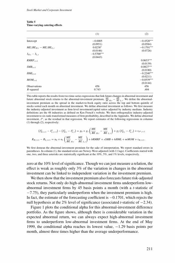
Table 5 reports the results for those two time-series regressions. Since weform the left-hand-side variable in the first regression from information that onlychanges annually, we expect some degree of autocorrelation in the errors andthus report Newey-West (1987) t-statistics adjusted for 11 lags. We know thatfor the return-forecasting regression, the small-sample p-values obtained fromthe usual student t-test tend to over-reject the null (Stambaugh, 1999) whenthe forecasting variable is persistent with shocks that are negatively correlatedwith return shocks. However, in our case, our forecasting variable has a muchlower persistence (an AR(1) coefficient of 0.9, not reported) than, for example,the dividend yield. Moreover, shocks to the investment premium variable arepositively correlated with the return shocks. Therefore, since the size distortionis minimal, we report OLS t-statistics for the second regression.17

We find evidence of catering effects using this approach. We first investigatewhether the investment premium forecasts subsequent changes in abnormalinvestment. The coefficient is 0.0238 with an associated t-statistic of 1.63,which rejects the null hypothesis that the coefficient is less than or equal to

17 We have confirmed that there is no size distortion in our hypothesis tests using the conditional-critical-valuefunction of Polk, Thompson, and Vuolteenaho (2006).

210


Table 5Time-varying catering effects

(1) (2)

Intercept −0.0005 −0.4520∗∗∗(0.0951) (0.0584)

ME/BEH,t − ME/BEL ,t 0.0238∗ −0.1701∗∗∗(0.0146) (0.0726)

IH,t − IL ,t −0.5700∗∗∗(0.0443)

RMRFt+1 0.0653∗∗∗(0.0139)

SMBt+1 0.0827∗∗∗(0.0180)

HMLt+1 −0.2240∗∗∗(0.0211)

MOMt+1 −0.0539∗∗∗(0.0144)

Observations 456 456R-squared 0.743 .404

This table reports the results from two time-series regressions that link future changes in abnormal investment andfuture abnormal stock returns to the abnormal-investment premium, ME

BE H,t − MEBE L ,t . We define the abnormal-

investment premium as the spread in the market-to-book equity ratio across the top and bottom quintile ofstocks sorted each month on abnormal investment. We define abnormal investment as follows. We first measurethe industry-adjusted investment as firm-level investment/capital ratios adjusted by industry medians. Industrydefinitions are the 48 industries as defined on Ken French’s website. We then orthogonalize industry-adjustedinvestment to six rank-transformed measures of firm profitability, described in the Appendix. We define abnormalinvestment, I a , as the residual in that regression. We report estimates of the following regressions in columns(1) through (2), respectively:

(I a

H,t+1 − I aL ,t+1

) − (I a

H,t − I aL ,t

) = g0 + g1

(ME

BE H,t− ME

BE L ,t

)+ g2

(I a

H,t − I aL ,t

) + εI a ,t+1

RH,t+1 − RL ,t+1 = α0 + α1

(ME

BE H,t− ME

BE L ,t

)+ bRMRF + sSMB + hHML + mMOM + εR,t+1.

We first demean the abnormal-investment premium for the sake of interpretation. We report standard errors inparentheses. In column (1), the standard errors are Newey-West-adjusted (with 11 lags). Coefficients starred withone, two, and three asterisks are statistically significant at the 10%, 5%, and 1% levels, respectively.

zero at the 10% level of significance. Though we can just measure a relation, theeffect is weak as roughly only 3% of the variation in changes in the abnormalinvestment can be linked to independent variation in the investment premium.

We then show that the investment premium also forecasts future risk-adjustedstock returns. Not only do high-abnormal investment firms underperform low-abnormal investment firms by 45 basis points a month (with a t-statistic of−7.75), they particularly underperform when the investment premium is high.In fact, the estimate of the forecasting coefficient is −0.1701, which rejects thenull hypothesis at the 2% level of significance (associated t-statistic of −2.34).

Figure 1 plots the conditional alpha for this abnormal-investment differenceportfolio. As the figure shows, although there is considerable variation in theexpected abnormal return, we can always expect high-abnormal investmentfirms to underperform low-abnormal investment firms. At the end of May1999, the conditional alpha reaches its lowest value, −1.29 basis points permonth, almost three times higher than the average underperformance.

211


Figure 1Time-varying catering effectsThis figure shows the evolution of conditional alpha based on the regression in column (2) of Table 5,

RH,t+1 − RL ,t+1 = α0 + α1

(ME

BEH,t− ME

BEL ,t

)+ bRMRF + sSMB + hHML + mMOM + εR,t+1, (10)

which uses the spread in price-to-book across abnormal investment quintiles to predict the four-factor abnormalreturn on the abnormal-investment difference portfolio.

3. Conclusions

We present a framework based on Stein (1996) in which we show that a firm’sinvestment decision is affected by market (mis)valuation of the company, evenif new investment projects are not financed by new equity. If investors haveshort horizons, managers will rationally choose to invest in projects that areoverpriced and avoid projects that are underpriced, thus catering to sentimentin order to maximize near-term stock prices.

In the empirical part of the paper, we show that that when we control forinvestment opportunities and financial slack, variables that predict relativelylow stock returns are positively correlated with investment. We show that asa percentage of capital, a typical change in our mispricing proxy results inroughly a 2% change in the firm’s investment. Our model predicts that thegreater the degree of asymmetric information between firms and investors, thegreater should be these sensitivities. We find that is the case, as the effect isweaker for firms with relatively low R&D intensity.

Our model also predicts that the effects should be stronger for firms withshort-term investors. We find that this is also true, as the effect is stronger forfirms with relatively high share turnover.

212


The thrust of these results are generally consistent with Chirinko and Schaller(2001) and Baker, Stein, and Wurgler (2003), where sentiment also affects realinvestment. However, our results differ as the influence of sentiment on realinvestment works through a catering rather than an equity issuance channel.

We also show that patterns in the cross-section of average returns are con-sistent with those patterns in investment: firms with shorter shareholder hori-zons, and those whose assets are more difficult to value, cater more. Whenwe control for investment opportunities and other characteristics linked to re-turn predictability, we find that firms with high (low) investment have low(high) subsequent stock returns, and that this relation is stronger for firms withabove-median R&D intensity or above-median turnover.

Our main interpretation of the results is consistent with Stein’s (1996) hy-pothesis that short-horizon managers temporarily distort the firm’s investmentdecision and therefore misallocate resources. An alternative interpretation isthat our mispricing proxies measure unobserved (to the econometrician) ratio-nal variation in discount rates. On the one hand, stories explaining discretionalaccruals as a proxy for risk seem difficult, but on the other hand, it is puzzlingthat market forces do not discipline these investors’ biases. Nonetheless, ourresults provide a striking empirical regularity that associates firms’ investmentdecisions with a characteristic that apparently predicts future risk-adjustedreturns.

Finally, our paper focuses on just one important capital allocation decision.However, we could study other corporate decisions, such as hiring employeesor engaging in acquisition activity within this context. For example, Shleiferand Vishny (2003) argue that the cost of equity is a strong determinant ofmerger activity. Evidence consistent with this alternative channel is reported inRhodes-Kropf, Robinson, and Viswanathan (2004).

Appendix

Investment (It ) is capital expenditure (Compustat Item 128). Capital (Kt−1) is net property,plant, and equipment (Compustat Item 8). Qt−1 equals the market value of assets divided bythe book value of assets (Compustat Item 6). The market value of assets equals the book valueof assets plus the market value of common stock less the sum of book value of common stock(Compustat Item 6) and balance sheet deferred taxes (Compustat Item 74) in year t − 1. Cashflow (CFt−1) equals the sum of earnings before extraordinary items (Compustat Item 18) anddepreciation (Compustat Item 14) over beginning-of-year capital. Sales (Compustat Item 12) is netsales. The one-year expected profitability (Et−1[ROAt ]) is the median analyst year t − 1 forecast ofearnings in year t divided by the book value of assets (Compustat Item 6). The two-year expectedprofitability (Et−1[ROAt+1]) is the median analyst year t − 1 forecast of earnings in year t + 1divided by the book value of assets (Compustat Item 6) in year t − 1. The five-year expectedprofitability (Et−1[ROAt+4]) is the median analyst year t − 1 forecast of earnings in year t + 4divided by the book value of assets (Compustat Item 6) in year t − 1. R&D intensity is R&Dexpense (Compustat Item 46) over the book value of assets (Compustat Item 6). We ignore firmswith negative accounting numbers for book assets, capital, or investment. Because the observationsprobably represent data errors, we drop those firms that have extreme values for the accountingratios we study.

213


We construct discretionary accruals following Chan et al. (2001). Accruals (ACCRt ) equal thechange in accounts receivable (Compustat Item 2) plus the change in inventories (Compustat Item 3)plus the change in other current assets (Compustat Item 68) minus the change in accounts payable(Compustat Item 70) minus the change in other current liabilities (Compustat Item 72) minusdepreciation (Compustat Item 178). We scale accruals by total assets (the average of CompustatItem 6 at the beginning and end of the fiscal year). We define the discretionary component ofaccruals as

DACCRt = ACCRt − NORMALACCRt , (11)

NORMALACCRi,t =( ∑5

k=1 ACCRi,t−k∑5k=1 SALESi,t−k

SALESi,t .

)(12)

Therefore, we model normal accruals as a constant proportion of firm sales.The price-to-book ratio we use to form portfolios in May of year t is book common equity for

the fiscal year ending in calendar year t − 1, divided by market equity at the end of May of yeart . We require the firm to have a valid past price-to-book ratio. Moreover, to eliminate likely dataerrors, we discard those firms with price-to-book ratio less than 0.01 and greater than 100. Whenusing Compustat as our source of accounting information, we require that the firm must be listedon Compustat for two years. This requirement alleviates most of the potential survivor bias due toCompustat backfilling data.

The Kaplan and Zingales (1997) index is: −1.001909*[(Item 18 + Item 14)/Item 8] +0.2826389*[(Item 6 + CRSP December Market Equity – Item 60 – Item 74)/Item 6] +3.139193*[(Item 9 + Item 34)/(Item 9 + Item 34 + Item 216)] −39.3678*[(Item 21 + Item 19)/Item8] −1.314759*[Item 1/Item 8]. Item numbers refer to Compustat annual data items. CompustatItem 8 is lagged.

We define BE as stockholders’ equity, plus balance sheet deferred taxes (Compustat Item 74) andinvestment tax credit (Compustat Item 208, set to zero if unavailable), plus postretirement benefitliabilities (Compustat Item 330, set to zero if unavailable), minus the book value of preferredstock. Depending on availability of preferred stock data, we use redemption (Compustat Item56), liquidation (Compustat Item 10), or par value (Compustat Item 130), in that order, for thebook value of preferred stock. We calculate stockholders’ equity as follows. We prefer to usethe the stockholders’ equity number reported by Moody’s or Compustat (Compustat Item 216).If neither is available, we measure stockholders’ equity as the book value of common equity(Compustat Item 60), plus the book value of preferred stock. (We add the preferred stock at thisstage, because later we subtract it in the book equity formula.) If common equity is not available,we compute stockholders’ equity as the book value of assets (Compustat Item 6) minus totalliabilities (Compustat Item 181), all from Compustat. To compute BE/ME, we match BE for allfiscal year-ends in calendar year t − 1 (1962–2001) with the firm’s market equity at the end of Mayyear t . Following Carhart (1997), momentum is the total gross return over the previous monthst − 2 to t − 12. Size is the market capitalization as of the end of month t − 1.

Our profitability controls in Section 2.5 that are used to generate abnormal investment are asfollows. Our first profitability control is D/BE, the ratio of dividends in year t to year t − 1 bookequity, for those firms with positive book equity. Fama and French (2000) is our motivation forthis variable. They point out that firms target dividends to the permanent component of earnings(Lintner, 1956; Miller and Modigliani, 1961; and others). We censor each firm’s D/BE ratio to therange (0,0.15) to limit the influence of near-zero book equity firms. The second profitability controlis a nondividend-paying dummy, DD, that is 0 for dividend payers and 1 for those firms not payingdividends. We use this dummy to capture any nonlinearity between expected profitability anddividends. Our third and fourth profitability controls are past long-term profitability and transitoryprofitability, which we include to capture the substantial mean reversion in profitability documentedby Fama and French. Long-term profitability is the three-year average clean-surplus profitability,ROE ≡ (BEt − BEt−3 + Dt−2 + Dt−1 + Dt )/(3 × BEt−3) We define transitory profitability as

214


ROE − ROE, where ROE is current profitability and is equal to (BEt − BEt−1 + Dt )/(BEt−1).Our fifth profitability control is a loss dummy that captures the fact that firms that are losingmoney typically continue to do poorly in the future. Finally, to capture the phenomenon that lowconcentration within industry should signal intense competition and thus lower profitability, weinclude a Herfindahl index of equity market capitalizations for the top five firms in each two-digitSIC code industry.

ReferencesAbel, A., and O. Blanchard. 1986. The Present Value of Profits and Cyclical Movements in Investment. Econo-metrica 54:249–74.

Abel, A., and J. Eberly. 2002. Investment and Q with Fixed Costs: An Empirical Analysis. Working Paper,Northwestern University.

Baker, M., R. Ruback, and J. Wurgler. forthcoming. Behavioral Corporate Finance: A Survey, in Espen Eckbo(ed.), The Handbook of Corporate Finance: Empirical Corporate Finance. New York: Elsevier/North-Holland.

Baker, M., J. Stein, and J. Wurgler. 2003. When Does the Market Matter? Stock Prices and the Investment ofEquity-Dependent Firms. Quarterly Journal of Economics 118(3):969–1005.

Baker, M., and J. Wurgler. 2000. The Equity Share in New Issues and Aggregate Stock Returns. Journal ofFinance 55:2219–57.

Baker, M., and J. Wurgler. 2002. Market Timing and Capital Structure. Journal of Finance 57:1–32.

Baker, M., and J. Wurgler. 2004. A Catering Theory of Dividends. Journal of Finance 59:271–88.

Barro, R. 1990. The Stock Market and Investment. The Review of Financial Studies 3:115–31.

Bergstresser, D., M. A. Desai, and J. Rauh. 2004. Earnings Manipulation and Managerial Investment Decisions:Evidence from Sponsored Pension Plans. Working Paper No. 10543, NBER.

Blanchard, O., C. Rhee, and L. Summers. 1993. The Stock Market, Profit and Investment. Quarterly Journal ofEconomics 108(1):115–36.

Bond, S., and J. Cummins. 2000. The Stock Market and Investment in the New Economy: Some Tangible Factsand Intangible Fictions. Brookings Papers on Economic Activity 2000(1), 61–124.

Carhart, M. 1997. On Persistence in Mutual Fund Performance. Journal of Finance 52(1):57–82.

Chan, K., K. C. Chan, N. Jegadeesh, and J. Lakonishok. 2001. Earnings Quality and Stock Returns. NBER,Working Paper No. 8308.

Chirinko, R., and H. Schaller. 2001. Business Fixed Investment and “Bubbles” : The Japanese Case. AmericanEconomic Review 91:663–80.

Cochrane, J. 1991. Production-Based Asset Pricing and the Link Between Stock Returns and Economic Fluctu-ations. Journal of Finance 46:209–37.

Cohen, R., C. Polk, and T. Vuolteenaho. 2003. The Value Spread. Journal of Finance 58:609–41.

Cooper, M. J., O. Dimitrov, and P. R. Rau. 2001. A Rose.com by Any Other Name. Journal of Finance 56:2371–88.

Cooper, M. J., A. Khorana, I. Osobov, A. Patel, and P. R. Rau. 2005. Managerial Actions in Response to aMarket Downturn: Valuation Effects of Name Changes in the Dot.com Decline. Journal of Corporate Finance11:319–35

D’Avolio, E. Gildor, and A. Shleifer. 2002. Technology, Information Production, and Market Efficiency, inEconomic Policy For The Information Economy, A Symposium Sponsored by The Federal Reserve Bank ofKansas City.

Daniel, K., and S. Titman. 2006. Market Reactions to Tangible and Intangible Information. Journal of Finance61(4):1605–43.

215


Dow, J., and G. Gorton. 1997. Stock Market Efficiency and Economic Efficiency: Is There a Connection? Journalof Finance 52:1087–1129.

Erickson, T., and T. M. Whited. 2000. Measurement Error and the Relationship between Investment and Q.Journal of Political Economy 108:1027–57.

Erickson, T., and T. M. Whited. 2002. Two-step GMM Estimation of the Errors-in-variables Model UsingHigh-order Moments. Econometric Theory 18:776–99.

Fama, E. 1970. Efficient Capital Markets: A Review of Theory and Empirical Work. Journal of Finance 25:383–423.

Fama, E., and K. French. 1993. Common Risk Factors in the Returns on Stocks and Bonds. Journal of FinancialEconomics 33:3–56.

Fama, E., and K. French. 2000. Forecasting Profitability and Earnings. Journal of Business 72:161–75.

Fama, E., and J. MacBeth. 1973. Risk, Return, and Equilibrium: Empirical Tests. Journal of Political Economy281:607–36.

Froot, K., D. Scharfstein, and J. Stein. 1994. A Framework for Risk Management. Harvard Business Review72:91–102.

Gaspar, J. M., M. Massa, and P. Matos. 2005. Shareholder Investment Horizons and the Market for CorporateControl. Journal of Financial Economics 76(1):135–65.

Gilchrist, S., and C. Himmelberg. 1995. Evidence on the Role of Cash Flow for Investment. Journal of MonetaryEconomics 36:541–72.

Gilchrist, S., C. Himmelberg, and G. Huberman. 2005. Do Stock Price Bubbles Influence Corporate Investment?Journal of Monetary Economics 52:805–27.

Hand, J. 1990. Did Firms Undertake Debt-equity Swaps for an Accounting Paper Profit or True Financial Gain?The Accounting Review 64:587–623.

Hribar, P., and D. Collins. 2002. Errors in Estimating Accruals: Implications for Empirical Research. Journal ofAccounting Research 40:105–34.

Jensen, M. C. 2005. Agency Costs of Overvalued Equity. Working Paper No. 04-26, Harvard NOM; FinanceWorking Paper No. 39/2004, ECGI, available at http://ssrn.com/abstract=480421.

Jones, J. 1991. Earnings Management During Import Relief Investigation. Journal of Accouting Research 29:193–228.

Kaplan, S., and L. Zingales. 1997. Do Financing Constraints Explain Why Investment is Correlated with CashFlow? Quarterly Journal of Economics 112:168–216.

Lamont, O. 2000. Investment Plans and Stock Returns. Journal of Finance 55:2719–45.

Lintner, J. 1956. The Distribution of Incomes of Corporations among Dividends, Retained Earnings and Taxes.American Economic Review 46:97–113.

Maines, L., and J. Hand. 1996. Individuals’ Perceptions and Misperceptions of the Time Series Properties ofQuarterly Earnings. The Accounting Review 71:317–36.

Mayer, C. 1988. A New Test of Capital Structure. European Economic Review 32:1167–89.

Mayer, C., and O. Sussman. 2003. New Issues in Corporate Finance. Working Paper, Oxford University.

Miller, M., and F. Modigliani. 1961. Dividend policy, growth, and the valuation of shares. Journal of Business34:411–33.

Morck, R., A. Shleifer, and R. Vishny. 1990. The Stock Market and Investment: Is the Market a Sideshow?.Brookings Papers on Economic Activity 2:157–215.

216


Newey, W. K., and K. D. West. 1987. A Simple, Positive Semi-Definite, Heteroskedasticity and AutocorrelationConsistent Covariance Matrix. Econometrica 55(3):703–08.

Panageas, S. 2005. The Neoclassical q Theory of Investment in Speculative Markets. Mimeo, The WhartonSchool, University of Pennsylvania.

Polk, C., and P. Sapienza. 2004. The Real Effects of Investor Sentiment. Working Paper No. 10563, NBER.

Polk, C., S. Thompson, and T. Vuolteenaho. 2006. Cross-sectional Forecasts of the Equity Premium. Journal ofFinancial Economics 81:101–41.

Rajan, R., and L. Zingales. 1995. What Do We Know about Capital Structure? Some Evidence from InternationalData. Journal of Finance 50:1421–60.

Rhodes-Kropf, M., D. Robinson, and S. Viswanathan. 2004. Valuation Waves and Merger Activity: The EmpiricalEvidence. Working Paper, Columbia Business School.

Shleifer, A., and R. Vishny. 1990. Equilibrium Short Horizons of Investors and Firms. American EconomicReview Papers and Proceedings 80:148–53.

Shleifer, A., and R. Vishny. 2003. Stock Market Driven Acquisitions. Journal of Financial Economics 70:295–311.

Sloan, R. 1996. Do Stock Prices Fully Reflect Information in Accruals and Cash Flows about Future Earnings?The Accounting Review 71:289–315.

Stambaugh, R. F. 1999. Predictive Regressions. Journal of Financial Economics 54:375–421.

Stein, J. 1988. Takeover Threats and Managerial Myopia. Journal of Political Economy 96:61–80.

Stein, J. 1996. Rational Capital Budgeting in an Irrational World. Journal of Business 69:429–55.

Stein, J. 2003. Agency, Information and Corporate Investment, in G. Constantinides, M. Harris, and R. Stulz(eds), The Handbook of the Economics of Finance. New York: Elsevier/North-Holland, pp. 111–65.

Teoh, S. H., I. Welch, and T. J. Wong. 1998a. Earnings Management and the Long-term Market Performance ofInitial Public Offerings. Journal of Finance 53:1935–74.

Teoh, S. H., I. Welch, and T. J. Wong. 1998b. Earnings Management and the Underperformance of SeasonedEquity Offerings. Journal of Financial Economics 50:63–99.

Titman, S., K. C. J. Wei, and F. Xie. 2004. Capital Investments and Stock Returns. Journal of Financial andQuantitative Analysis 39:677–700.

217

Documents

The Stock Market and Corporate Investment: A Test of ... Stock Market and Corporate Investment: A Test of Catering Theory Christopher Polk London School of Economics Paola Sapienza