THE STATUS OF THE QUIJOTE MULTI-FREQUENCY INSTRUMENTdigital.csic.es/bitstream/10261/109140/1/The status of the QUIJOTE.pdf · Here we present the current status of the QUIJOTE multi-frequency

THE STATUS OF THE QUIJOTE MULTI-FREQUENCY INSTRUMENT

R.J. Hoyland*a, M. Aguiar-Gonzáleza, B. Ajac, J. Ariñof, E. Artalc, R. B. Barreirob, E. J. Blackhurstd, J. Cagigasc, J. L. Cano de Diegoc, F. J. Casasb, R. J. Davisd, C. Dickinsond, B. E. Arriagaf,

R. Fernandez-Cobosb, L. de la Fuenteb, R. Génova-Santosa, A. Gómezf, C. Gomezf, F. Gómez-Reñascoa, K. Graingee, S. Harperd, D. Herranb, J. M. Herrerosa, G A. Herrerag, M. P. Hobsone, A. N.

Lasenbye , M Lopez-Caniegob, C. López-Caraballoa, B. Maffeid, E. Martinez-Gonzalezb, M. McCullochd , S. Melhuishd , A. Mediavilla c, G. Murgaf, D. Ortizb, L. Piccirillod, G. Pisanod, R.

Rebolo-Lópeza, J. A. Rubiño-Martina, J. Luis Ruizf,V.Sanchez de la Rosaa, R. Sanquircef, A. Vega-Morenoa, P. Vielvab, T. Viera-Curbeloa, E.Villac, A. Vizcargüenagaf, R. A.Watsond,

a Instituto de Astrofisica de Canarias (IAC), C/Via Lactea, s/n, E-38200, La

Laguna, Tenerife, Spain. 00349226005200 bInstituto de Fisica de Cantabria (IFCA), CSIC-Univ. de Cantabria, Avda. los

Castros, s/n, E-39005 Santander, Spain 0034942201459 cDepartamento de Ingenieria de COMunicaciones (DICOM), Laboratorios de I+D de

Telecomunicaciones, Plaza de la Ciencia s/n, E-39005 Santander, SpaindJodrell Bank Centre for Astrophysics, School of Physics and Astronomy,

University of Manchester, Oxford Road, Manchester M13 9PL, UK 0044161 275 4194 eAstrophysics Group, Cavendish Laboratory, University of Cambridge, Madingley

Road, Cambridge CB3 0HE 0044 1223 339992fIDOM, Avda. Lehendakari Aguirre, 3, E-48014 Bilbao, Spain 0034944797600

gGuillermo Herrera, C/Antonio del Castillo, Edif. Castillo, # 3, Portal 2, 2º A. Tegueste, C.P. 38280 Tenerife - España 0034 660619163

;

ABSTRACT

The QUIJOTE-CMB project has been described in previous publications. Here we present the current status of the QUIJOTE multi-frequency instrument (MFI) with five separate polarimeters (providing 5 independent sky pixels): two which operate at 10-14 GHz, two which operate at 16-20 GHz, and a central polarimeter at 30 GHz. The optical arrangement includes 5 conical corrugated feedhorns staring into a dual reflector crossed-draconian system, which provides optimal cross-polarization properties (designed to be < !35 dB) and symmetric beams. Each horn feeds a novel cryogenic on-axis rotating polar modulator which can rotate at a speed of up to 1 Hz. The science driver for this first instrument is the characterization of the galactic emission. The polarimeters use the polar modulator to derive linear polar parameters Q, U and I and switch out various systematics. The detection system provides optimum sensitivity through 2 correlated and 2 total power channels. The system is calibrated using bright polarized celestial sources and through a secondary calibration source and antenna. The acquisition system, telescope control and housekeeping are all linked through a real-time gigabit Ethernet network. All communication, power and helium gas are passed through a central rotary joint. The time stamp is synchronized to a GPS time signal. The acquisition software is based on PLCs written in Beckhoffs TwinCat and ethercat. The user interface is written in LABVIEW. The status of the QUIJOTE MFI will be presented including pre-commissioning results and laboratory testing.

Keywords: polarization, CMBr, instrumentation, spectrometer, foregrounds, B-modes, mapping

!"##"$%&%'()*+,$"##"$%&%'()-./)0-'12.3'-'%/)4%&%5&6'7)-./)2.7&'+$%.&-&"6.)36')87&'6.6$9):2()%/"&%/),9);-9.%)*<)=6##-./()>6.-7)?$+"/@".-7()A'65<)63)*A2B):6#<)CDEF()

CDEFGG)H)FIJF)*A2B)K)LLL)56/%M)IFNN1NCOPQJFQRJC)K)/6"M)JI<JJJNQJF<SFEGDS

A'65<)63)*A2B):6#<)CDEF))CDEFGG1J

Downloaded From: http://proceedings.spiedigitallibrary.org/ on 11/13/2012 Terms of Use: http://spiedl.org/terms

1. INTRODUCTION

The study of the anisotropy in the Cosmic Microwave Background (CMB) provides a powerful tool to obtain high-precision constraints on the basic cosmological parameters that describe our Universe. For this reason several experiments have been mapping the intensity of these anisotropies over the last decades with increasingly higher

sensitivities. All these data have successfully confirmed the !CDM paradigm. The Planck ESA satellite [1], which is currently flying, will produce full-sky maps with unprecedented angular resolution and sensitivity. With the completion of these observations there has been a growing interest in studying the polarization of the CMB. Despite the fact that the polar signal is more than two orders of magnitude below that of total intensity, it is now possible to study these signals thanks to the increasing sensitivity of the instrumentation. The CMB polarization pattern is normally decomposed into the E-modes (curl-free component) and the B-modes (curl component). The E-modes were first detected by the DASI experiment [2]. The amplitude of the B modes is expected to be around an order of magnitude lower and remains undetected. Its detection would however be an important milestone in cosmology, as it would confirm the presence of gravitational waves in the primordial Universe, which would have been created by inflation, an epoch of exponential expansion of the early Universe. Furthermore, the determination of the amplitude of the B-modes will give information about the energy scale at which inflation occurred. For the previous reasons, several experiments have been designed in the last few years to observe the CMB polarization. These experiments, apart from having high sensitivity, will need to be complemented with an accurate characterization of the polarization of the Galactic foregrounds, whose amplitude is higher than the B-mode signal. The QUIJOTE (Q-U-I JOint TEnerife) CMB experiment is one of these current observational efforts. The scientific objectives of this project

are two-fold: i) to detect the imprint of the primordial B-mode signal if it has an amplitude r"0.05 [3], and ii) to characterize the polarized foregrounds at low frequencies. This experiment will probably be unique in what concerns the second of these goals, as it is the only one observing at low frequencies (<20 GHz), and therefore will provide essential information about the polarization of the synchrotron and the anomalous microwave emissions, the two main polarized foregrounds emitting at low frequencies. These measurements will be complemented, at high frequencies (>100 GHz), by measurements from the Planck mission, that will allow the characterization of the polarization in the thermal dust emission, another important foreground which is dominant at high frequency. The QUIJOTE-CMB experiment is a scientific collaboration between the Instituto de Astrofísica de Canarias, the Instituto de Física de Cantabria, the IDOM company, and the universities of Cantabria, Manchester and Cambridge. The whole project is made up of two phases. Phase I includes the construction of a first telescope (QT1) and two instruments: the multi-frequency instrument (MFI), operating at 10-30 GHz, and the thirty-gigahertz instrument (TGI). Phase II includes the construction of a second telescope (QT2) and a third instrument, the so-called forty-gigahertz instrument (FGI). The MFI will be dedicated primarily to the characterization of the polarized foregrounds, whereas the TGI and the FGI will be focused on B-mode science. The two telescopes will be situated in the Teide Observatory (Tenerife, Spain). At the moment of writing, the QT1 has already been deployed at the observatory, and will be commissioned with the MFI during summer 2012. More specific details about this project, its instrumental setup, and its scientific goals, are given in the accompanying article [3]. Further details about the MFI control system are given in [4]. In this article we present the status of the MFI.

2. THE QUIJOTE (MFI) INSTRUMENT DESIGN

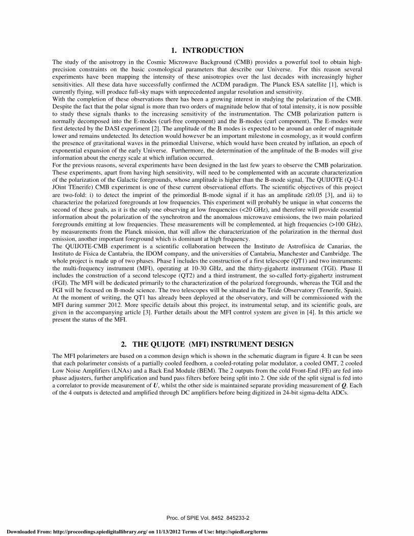
The MFI polarimeters are based on a common design which is shown in the schematic diagram in figure 4. It can be seen that each polarimeter consists of a partially cooled feedhorn, a cooled-rotating polar modulator, a cooled OMT, 2 cooled Low Noise Amplifiers (LNAs) and a Back End Module (BEM). The 2 outputs from the cold Front-End (FE) are fed into phase adjusters, further amplification and band pass filters before being split into 2. One side of the split signal is fed into a correlator to provide measurement of U, whilst the other side is maintained separate providing measurement of Q. Each of the 4 outputs is detected and amplified through DC amplifiers before being digitized in 24-bit sigma-delta ADCs.

A'65<)63)*A2B):6#<)CDEF))CDEFGG1F


0

Figure 4. A schematic diagram of the MFI polarimeter configuration.

Rotation of the polar modulator causes the outputs to be interchanged between Q and U. Sufficiently rapid rotation (>40Hz) of the polar modulator allows a complete removal of 1/f noise from the measurement of Q and U for all the MFI frequencies. This also allows complete independent Q,U and I measurement for each of the 4 outputs.

2.1 The general layout of instrument

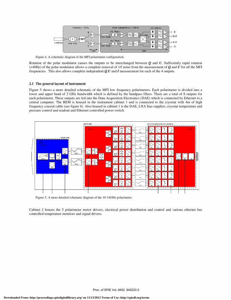
Figure 5 shows a more detailed schematic of the MFI low frequency polarimeters. Each polarimeter is divided into a lower and upper band of 2 GHz bandwidth which is defined by the bandpass filters. There are a total of 8 outputs for each polarimeter. These outputs are fed into the Data Acquisition Electronics (DAE) which is connected by Ethernet to a central computer. The BEM is housed in the instrument cabinet 1 and is connected to the cryostat with 4m of high frequency coaxial cable (see figure 6). Also housed in cabinet 1 is the DAE, LNA bias supplies, cryostat temperature and pressure control and readout and Ethernet controlled power switch.

Figure 5. A more detailed schematic diagram of the 10-14GHz polarimeter.

Cabinet 2 houses the 5 polarimeter motor drivers, electrical power distribution and control and various ethernet bus controlled temperature monitors and signal drivers.

A'65<)63)*A2B):6#<)CDEF))CDEFGG1G


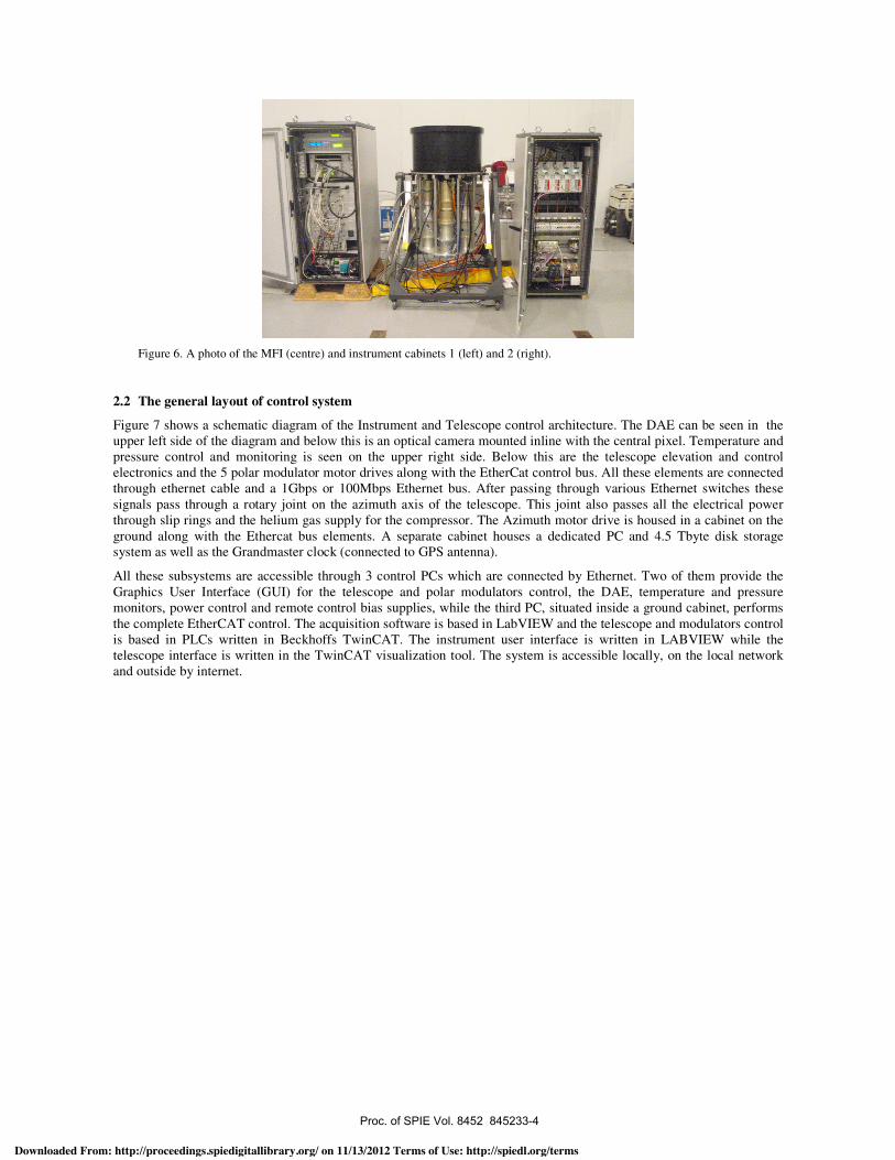
Figure 6. A photo of the MFI (centre) and instrument cabinets 1 (left) and 2 (right).

2.2 The general layout of control system

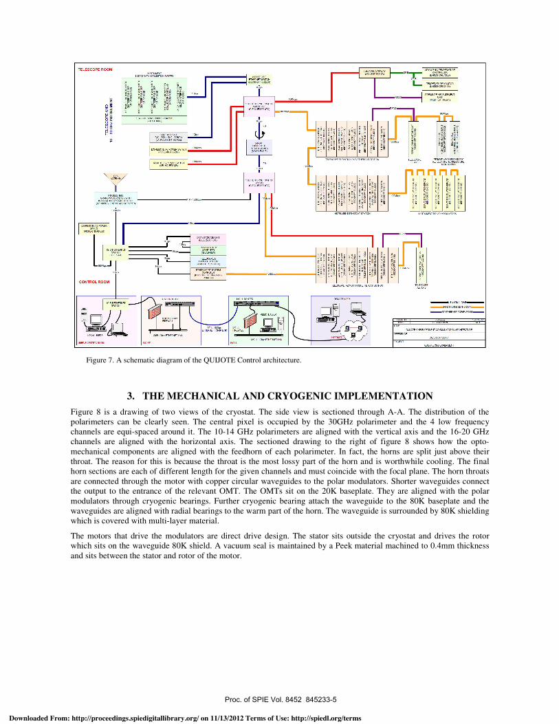
Figure 7 shows a schematic diagram of the Instrument and Telescope control architecture. The DAE can be seen in the upper left side of the diagram and below this is an optical camera mounted inline with the central pixel. Temperature and pressure control and monitoring is seen on the upper right side. Below this are the telescope elevation and control electronics and the 5 polar modulator motor drives along with the EtherCat control bus. All these elements are connected through ethernet cable and a 1Gbps or 100Mbps Ethernet bus. After passing through various Ethernet switches these signals pass through a rotary joint on the azimuth axis of the telescope. This joint also passes all the electrical power through slip rings and the helium gas supply for the compressor. The Azimuth motor drive is housed in a cabinet on the ground along with the Ethercat bus elements. A separate cabinet houses a dedicated PC and 4.5 Tbyte disk storage system as well as the Grandmaster clock (connected to GPS antenna).

All these subsystems are accessible through 3 control PCs which are connected by Ethernet. Two of them provide the Graphics User Interface (GUI) for the telescope and polar modulators control, the DAE, temperature and pressure monitors, power control and remote control bias supplies, while the third PC, situated inside a ground cabinet, performs the complete EtherCAT control. The acquisition software is based in LabVIEW and the telescope and modulators control is based in PLCs written in Beckhoffs TwinCAT. The instrument user interface is written in LABVIEW while the telescope interface is written in the TwinCAT visualization tool. The system is accessible locally, on the local network and outside by internet.

A'65<)63)*A2B):6#<)CDEF))CDEFGG1D


DC

LIN9IC

flCISN

I HO

DC

- DC

DN

V 9dOO

S9191

b H

1

Figure 7. A schematic diagram of the QUIJOTE Control architecture.

3. THE MECHANICAL AND CRYOGENIC IMPLEMENTATION

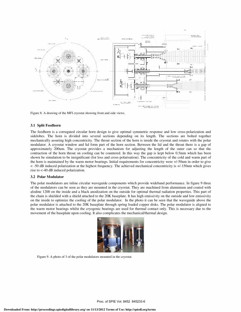
Figure 8 is a drawing of two views of the cryostat. The side view is sectioned through A-A. The distribution of the polarimeters can be clearly seen. The central pixel is occupied by the 30GHz polarimeter and the 4 low frequency channels are equi-spaced around it. The 10-14 GHz polarimeters are aligned with the vertical axis and the 16-20 GHz channels are aligned with the horizontal axis. The sectioned drawing to the right of figure 8 shows how the opto-mechanical components are aligned with the feedhorn of each polarimeter. In fact, the horns are split just above their throat. The reason for this is because the throat is the most lossy part of the horn and is worthwhile cooling. The final horn sections are each of different length for the given channels and must coincide with the focal plane. The horn throats are connected through the motor with copper circular waveguides to the polar modulators. Shorter waveguides connect the output to the entrance of the relevant OMT. The OMTs sit on the 20K baseplate. They are aligned with the polar modulators through cryogenic bearings. Further cryogenic bearing attach the waveguide to the 80K baseplate and the waveguides are aligned with radial bearings to the warm part of the horn. The waveguide is surrounded by 80K shielding which is covered with multi-layer material.

The motors that drive the modulators are direct drive design. The stator sits outside the cryostat and drives the rotor which sits on the waveguide 80K shield. A vacuum seal is maintained by a Peek material machined to 0.4mm thickness and sits between the stator and rotor of the motor.

A'65<)63)*A2B):6#<)CDEF))CDEFGG1E


A

Figure 8. A drawing of the MFI cryostat showing front and side views.

3.1 Split Feedhorn

The feedhorn is a corrugated circular horn design to give optimal symmetric response and low cross-polarization and sidelobes. The horn is divided into several sections depending on its length. The sections are bolted together mechanically assuring high concentricity. The throat section of the horn is inside the cryostat and rotates with the polar modulator. A cryostat window and lid form part of the horn section. Between the lid and the throat there is a gap of approximately 200um. The cryostat provides a mechanism for adjusting the length of the outer can so that the contraction of the horn throat on cooling can be countered. In this way the gap is kept below 0.5mm which has been shown be simulation to be insignificant (for loss and cross-polarisation). The concentricity of the cold and warm part of the horn is maintained by the warm motor bearings. Initial requirements for concentricity were +/-50um in order to give < -50 dB induced polarization at the highest frequency. The achieved mechanical concentricity is +/-150um which gives rise to <-40 dB induced polarization.

3.2 Polar Modulator

The polar modulators are inline circular waveguide components which provide wideband performance. In figure 9 three of the modulators can be seen as they are mounted in the cryostat. They are machined from aluminium and coated with alodine 1200 on the inside and a black anodization on the outside for optimal thermal radiation properties. This part of the chain is shielded with a shield attached to the 20K baseplate. It has high emissivity on the outside and low emissivity on the inside to optimize the cooling of the polar modulator. In the photo it can be seen that the waveguide above the polar modulator is attached to the 20K baseplate through spring loaded copper disks. The polar modulator is aligned to the warm motor bearings whilst the cryogenic bearings are used for thermal contact only. This is necessary due to the movement of the baseplate upon cooling. It also complicates the mechanical/thermal design.

Figure 9. A photo of 3 of the polar modulators mounted in the cryostat

A'65<)63)*A2B):6#<)CDEF))CDEFGG1O


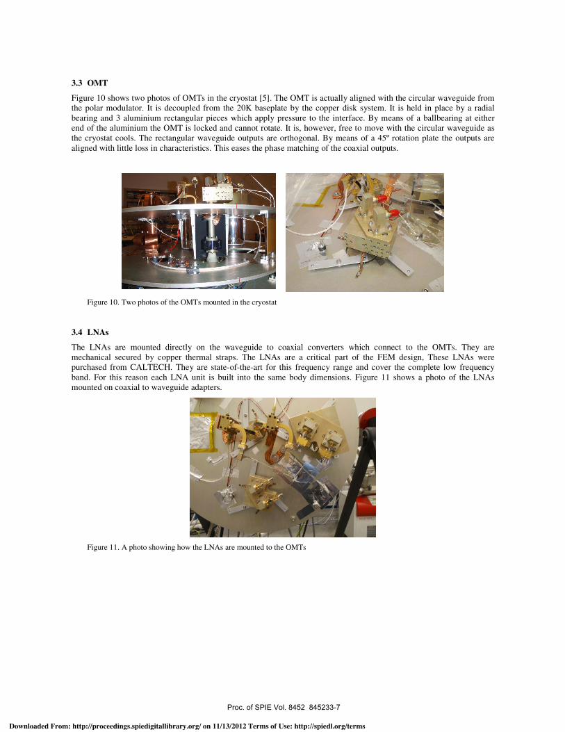
3.3 OMT

Figure 10 shows two photos of OMTs in the cryostat [5]. The OMT is actually aligned with the circular waveguide from the polar modulator. It is decoupled from the 20K baseplate by the copper disk system. It is held in place by a radial bearing and 3 aluminium rectangular pieces which apply pressure to the interface. By means of a ballbearing at either end of the aluminium the OMT is locked and cannot rotate. It is, however, free to move with the circular waveguide as the cryostat cools. The rectangular waveguide outputs are orthogonal. By means of a 45º rotation plate the outputs are aligned with little loss in characteristics. This eases the phase matching of the coaxial outputs.

Figure 10. Two photos of the OMTs mounted in the cryostat

3.4 LNAs

The LNAs are mounted directly on the waveguide to coaxial converters which connect to the OMTs. They are mechanical secured by copper thermal straps. The LNAs are a critical part of the FEM design, These LNAs were purchased from CALTECH. They are state-of-the-art for this frequency range and cover the complete low frequency band. For this reason each LNA unit is built into the same body dimensions. Figure 11 shows a photo of the LNAs mounted on coaxial to waveguide adapters.

Figure 11. A photo showing how the LNAs are mounted to the OMTs

A'65<)63)*A2B):6#<)CDEF))CDEFGG1N


-10

-15

-20

-25

-10

-l5

-20

-25

-30 -30 -300 5 10 5 20 25 0 5 10 15 20 25 0 5 0 IS 20 20

ArrgIe frees boresight,degrees Aregle roes boresighl, degrees Arrgle roes boresight degrees

10GHz 12GHz 14GHz

Feedhorn 10-14GHz 26-36GHz

Frequency,G Hz

10 12 14 27 31 35

Hornaperture, cm

180 64

Fartield. cm 220 259 303 74 79.5 95

Phasecentre, cm

0 0 0 0 0 0

FWHM (-3dB)

1 6.3 1 11 .2 1 6.8 1 2 1 2.4

FWHM (-8.7dB

26.9 21.9 18.4 26.4 22 19

Sidelobelevel

<-25dB <-25dB <-25dB <-25dB <-25dB -25dB

X-pol(45/90)

<-17dB <-25dB <-20dB <-22dB <-27dB <-20dB

4. MICROWAVE MEASUREMENTS OF SUBSYSTEMS

4.1 Opto-mechanical front-end

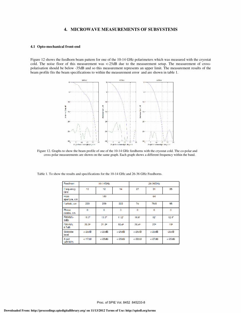
Figure 12 shows the feedhorn beam pattern for one of the 10-14 GHz polarimeters which was measured with the cryostat cold. The noise floor of this measurement was <-25dB due to the measurement setup. The measurement of cross-polarisation should be below -35dB and so this measurement represents an upper limit. The measurement results of the beam profile fits the beam specifications to within the measurement error and are shown in table 1.

Figure 12. Graphs to show the beam profile of one of the 10-14 GHz feedhorns with the cryostat cold. The co-polar and cross polar measurements are shown on the same graph. Each graph shows a different frequency within the band.

Table 1. To show the results and specifications for the 10-14 GHz and 26-36 GHz Feedhorns.

A'65<)63)*A2B):6#<)CDEF))CDEFGG1C


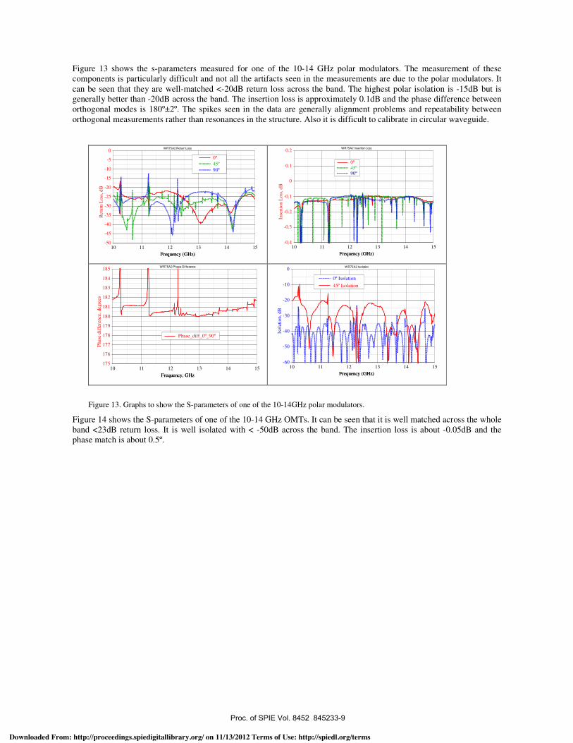
Figure 13 shows the s-parameters measured for one of the 10-14 GHz polar modulators. The measurement of these components is particularly difficult and not all the artifacts seen in the measurements are due to the polar modulators. It can be seen that they are well-matched <-20dB return loss across the band. The highest polar isolation is -15dB but is generally better than -20dB across the band. The insertion loss is approximately 0.1dB and the phase difference between orthogonal modes is 180º±2º. The spikes seen in the data are generally alignment problems and repeatability between orthogonal measurements rather than resonances in the structure. Also it is difficult to calibrate in circular waveguide.

Frequency (GHz)

Ret

urn

Loss

, d

B

-50

-45

-40

-35

-30

-25

-20

-15

-10

-5

0

Frequency (GHz)

10 11 12 13 14 15

WR75A2 Return Loss

0º

45º

90º

Frequency (GHz)

Inse

rtio

n L

oss

, dB

-0.4

-0.3

-0.2

-0.1

0

0.1

0.2

Frequency (GHz)

10 11 12 13 14 15

WR75A2 Insertion Loss

0º45º90º

Frequency, GHz

Pha

se d

iffe

renc

e, d

egre

es

175

176

177

178

179

180

181

182

183

184

185

Frequency, GHz

10 11 12 13 14 15

WR75A2 Phase Difference

Phase_diff_0º_90º

Frequency (GHz)

Iso

lati

on,

dB

-60

-50

-40

-30

-20

-10

0

Frequency (GHz)

10 11 12 13 14 15

WR75A2 Isolation

0º Isolation

45º Isolation

Figure 13. Graphs to show the S-parameters of one of the 10-14GHz polar modulators.

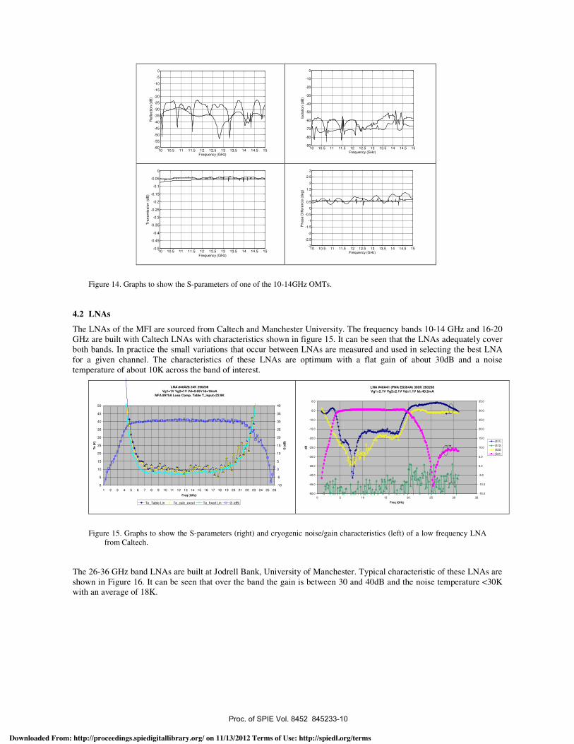
Figure 14 shows the S-parameters of one of the 10-14 GHz OMTs. It can be seen that it is well matched across the whole band <23dB return loss. It is well isolated with < -50dB across the band. The insertion loss is about -0.05dB and the phase match is about 0.5º.

A'65<)63)*A2B):6#<)CDEF))CDEFGG1S


10 10.5 11 11.5 12 12.5 13 13.5 14 14.5 15-60

-55

-50

-45

-40

-35

-30

-25

-20

-15

-10

-5

0

Frequency (GHz)R

efle

ctio

n (

dB

)

10 10.5 11 11.5 12 12.5 13 13.5 14 14.5 15

-90

-80

-70

-60

-50

-40

-30

-20

-10

0

Frequency (GHz)

Iso

latio

n (

dB

)

10 10.5 11 11.5 12 12.5 13 13.5 14 14.5 15-0.5

-0.45

-0.4

-0.35

-0.3

-0.25

-0.2

-0.15

-0.1

-0.05

0

Frequency (GHz)

Tra

nsm

issio

n (

dB

)

10 10.5 11 11.5 12 12.5 13 13.5 14 14.5 15

-3

-2.5

-2

-1.5

-1

-0.5

0

0.5

1

1.5

2

2.5

3

Frequency (GHz)

Ph

ase

Diff

ere

nce

(d

eg

)

Figure 14. Graphs to show the S-parameters of one of the 10-14GHz OMTs.

4.2 LNAs

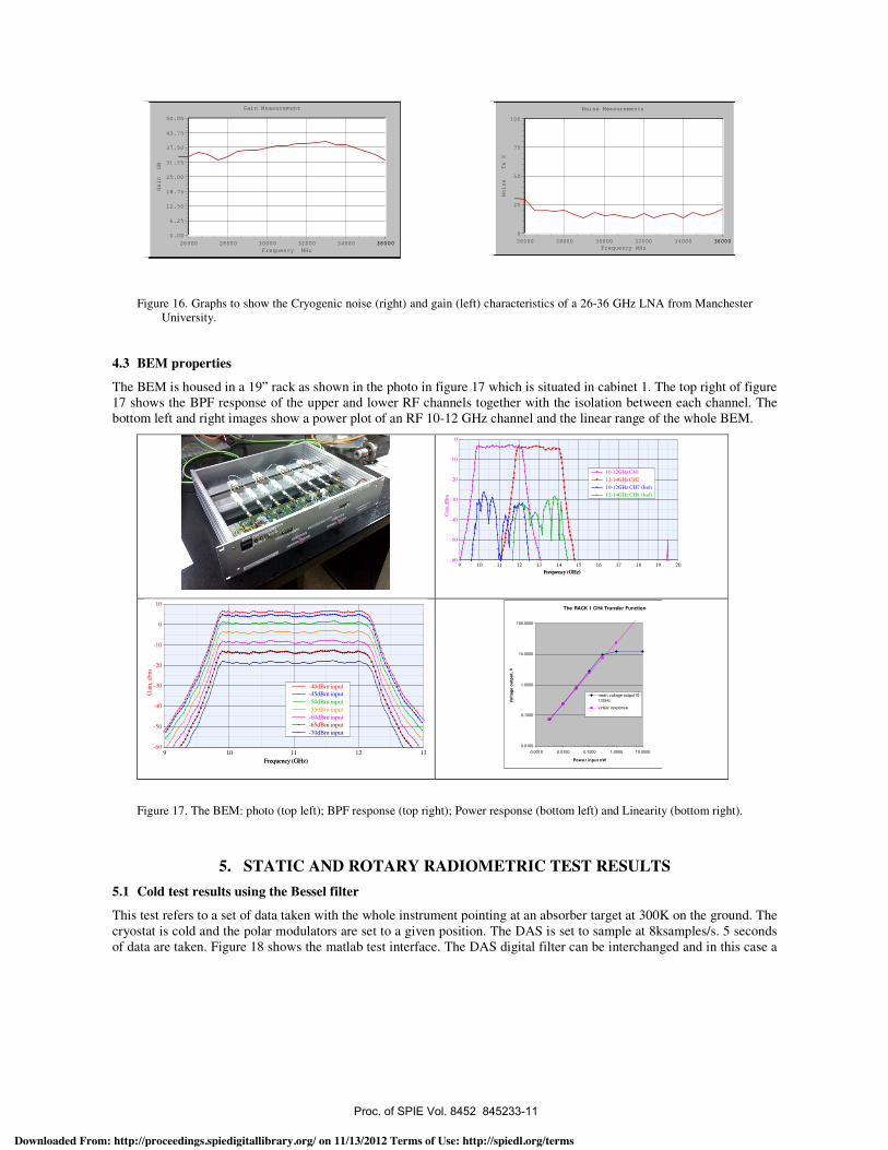
The LNAs of the MFI are sourced from Caltech and Manchester University. The frequency bands 10-14 GHz and 16-20 GHz are built with Caltech LNAs with characteristics shown in figure 15. It can be seen that the LNAs adequately cover both bands. In practice the small variations that occur between LNAs are measured and used in selecting the best LNA for a given channel. The characteristics of these LNAs are optimum with a flat gain of about 30dB and a noise temperature of about 10K across the band of interest.

Figure 15. Graphs to show the S-parameters (right) and cryogenic noise/gain characteristics (left) of a low frequency LNA from Caltech.

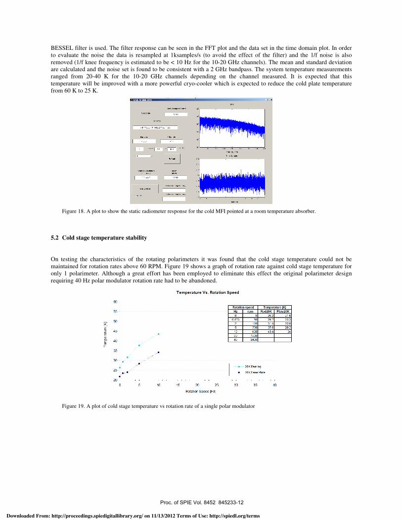
The 26-36 GHz band LNAs are built at Jodrell Bank, University of Manchester. Typical characteristic of these LNAs are shown in Figure 16. It can be seen that over the band the gain is between 30 and 40dB and the noise temperature <30K with an average of 18K.

LNA #40A28 24K 290208Vg1=1V Vg2=1V Vd=0.65V Id=16mA

NFA 8975A Loss Comp. Table T_input=22.9K

0

5

10

15

20

25

30

35

40

45

50

1 2 3 4 5 6 7 8 9 10 11 12 13 14 15 16 17 18 19 20 21 22 23 24 25 26

Freq (GHz)

Te

(K

)

-10

-5

0

5

10

15

20

25

30

35

40

G (

dB

)

Te_Table Lin Te_calc_excel Te_fixed Lin G (dB)

LNA #40A41 (PNA E8364A) 300K 260208Vg1=2.1V Vg2=2.1V Vd=1.1V Id=40.2mA

-50.0

-45.0

-40.0

-35.0

-30.0

-25.0

-20.0

-15.0

-10.0

-5.0

0.0

0 5 10 15 20 25 30 35

Freq (GHz)

dB

-15.0

-10.0

-5.0

0.0

5.0

10.0

15.0

20.0

25.0

30.0

35.0

|S11|

|S12|

|S22|

|S21|

A'65<)63)*A2B):6#<)CDEF))CDEFGG1JI


Gain Measurement

Frequency MHz

3600026000 28000 30000 32000 34000 36000

Gain dB

50.00

0.00

6.25

12.50

18.75

25.00

31.25

37.50

43.75

Noise Measurements

Frequency MHz

3600026000 28000 30000 32000 34000 36000

Noise Te K

100

0

25

50

75

Figure 16. Graphs to show the Cryogenic noise (right) and gain (left) characteristics of a 26-36 GHz LNA from Manchester University.

4.3 BEM properties

The BEM is housed in a 19” rack as shown in the photo in figure 17 which is situated in cabinet 1. The top right of figure 17 shows the BPF response of the upper and lower RF channels together with the isolation between each channel. The bottom left and right images show a power plot of an RF 10-12 GHz channel and the linear range of the whole BEM.

Frequency (GHz)

Gai

n,d

Bm

-60

-50

-40

-30

-20

-10

0

Frequency (GHz)

9 10 11 12 13 14 15 16 17 18 19 20

10-12GHz CH1

12-14GHz CH2

10-12GHz CH7 (Isol)

12-14GHz CH8 (Isol)

The RACK 1 CH4 Transfer Function

0.0100

0.1000

1.0000

10.0000

100.0000

0.0010 0.0100 0.1000 1.0000 10.0000

Power input nW

Vo

ltag

e o

utp

ut,

V

mean voltage output10-12GHz

Linear response

Figure 17. The BEM: photo (top left); BPF response (top right); Power response (bottom left) and Linearity (bottom right).

5. STATIC AND ROTARY RADIOMETRIC TEST RESULTS

5.1 Cold test results using the Bessel filter

This test refers to a set of data taken with the whole instrument pointing at an absorber target at 300K on the ground. The cryostat is cold and the polar modulators are set to a given position. The DAS is set to sample at 8ksamples/s. 5 seconds of data are taken. Figure 18 shows the matlab test interface. The DAS digital filter can be interchanged and in this case a

Frequency (GHz)

Gai

n, d

bm

-60

-50

-40

-30

-20

-10

0

10

Frequency (GHz)

9 10 11 12 13

-40dBm input-45dBm input

-50dBm input

-55dBm input

-60dBm input-65dBm input

-70dBm input

A'65<)63)*A2B):6#<)CDEF))CDEFGG1JJ


.30 --,

25

Temperature Vs. Rotation Speed

5 10 15 20 25

Rotation Speed [Hz]

30 35 40

Rotation speed Tempe ature (K]Hz rpm Rod2tK Plate2tK0 0 26.2 21.6

0.833 50 29.2 23.32 120 31.5 23.85 300 37.6 28.2

10 600 43.4 3420 120040 2400

60

55

50

5 45

40I-

35

--s--- 20K Bearing

-------20K Base Plate

II-

BESSEL filter is used. The filter response can be seen in the FFT plot and the data set in the time domain plot. In order to evaluate the noise the data is resampled at 1ksamples/s (to avoid the effect of the filter) and the 1/f noise is also removed (1/f knee frequency is estimated to be < 10 Hz for the 10-20 GHz channels). The mean and standard deviation are calculated and the noise set is found to be consistent with a 2 GHz bandpass. The system temperature measurements ranged from 20-40 K for the 10-20 GHz channels depending on the channel measured. It is expected that this temperature will be improved with a more powerful cryo-cooler which is expected to reduce the cold plate temperature from 60 K to 25 K.

Figure 18. A plot to show the static radiometer response for the cold MFI pointed at a room temperature absorber.

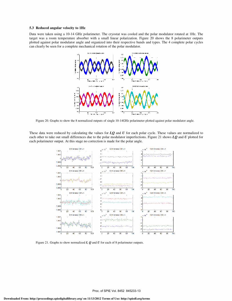
5.2 Cold stage temperature stability

On testing the characteristics of the rotating polarimeters it was found that the cold stage temperature could not be maintained for rotation rates above 60 RPM. Figure 19 shows a graph of rotation rate against cold stage temperature for only 1 polarimeter. Although a great effort has been employed to eliminate this effect the original polarimeter design requiring 40 Hz polar modulator rotation rate had to be abandoned.

Figure 19. A plot of cold stage temperature vs rotation rate of a single polar modulator

A'65<)63)*A2B):6#<)CDEF))CDEFGG1JF


1.002

1.001

0.999

0.998

1.002

1.001

0.999

0.998

1.002

1.001

0.999

0.998

1.002

1.001

0.999

0.998

I(250norn) CHI*2

4\ lq' \f)%!\ 1,

20 40 60 80 100

I(250nor) CH3.4

20 40 60 80 100

I(250nor) CH5*6

20 40 60 80 100

J(250ror) CH7*8

20 40 60 80 100

x io O(250norr) CH5+6

0 20 40 60 80

O(250ror) CH7+8

O(250norr) CHI*2

100

U(250,orn) CHI,2

U(250,orr) CH3,4

lo U(250orr) CH7.8

5.3 Reduced angular velocity to 1Hz

Data were taken using a 10-14 GHz polarimeter. The cryostat was cooled and the polar modulator rotated at 1Hz. The target was a room temperature absorber with a small linear polarization. Figure 20 shows the 8 polarimeter outputs plotted against polar modulator angle and organized into their respective bands and types. The 4 complete polar cycles can clearly be seen for a complete mechanical rotation of the polar modulator.

Figure 20. Graphs to show the 8 normalized outputs of single 10-14GHz polarimeter plotted against polar modulator angle.

These data were reduced by calculating the values for I,Q and U for each polar cycle. These values are normalized to each other to take out small differences due to the polar modulator imperfections. Figure 21 shows I,Q and U plotted for each polarimeter output. At this stage no correction is made for the polar angle.

Figure 21. Graphs to show normalized I, Q and U for each of 8 polarimeter outputs.

A'65<)63)*A2B):6#<)CDEF))CDEFGG1JG


The expected level of sigma found in these plots is 1.5 times that expected for 2 GHz bandwidth and 250ms sample rate. This excess is small and in any case only affects the large scale structure in a given observation. The low frequency channels can make use of this technique without large degradation in the observations.

5.4 Discrete switching of Q/U 2 and 4 position

A complementary fallback technique is to use a slower switch rate whereby the polar modulator is discretely switched by 22.5º every 30 seconds. There is almost no 1/f rejection in this type of switching and so the difference between the two correlated polar channels must be taken. This difference gives a voltage proportional to Q at 22.5º and U at 0º.The voltage is stable with respect to 1/f fluctuations (to 1st order) because the channels have been correlated and the output contains the 1/f from both the LNAs. Switching the polar modulator between 0º and 22.5º provides a measurement of both Q and U. The disadvantage is that the total power channels cannot be used since they are not correlated. This implies a loss of 2 in the sensitivity which is comparable to the los in sensitivity for the continuous method. The systematics are expected to be higher using this method because two channels have to be used and do not have the exact same bandpass.

Results of a Jones/Muller type analysis [6] showed that switching between only 2 positions was not enough to eliminate certain polar modulator imperfections, however, by switching between 4 positions: 0º, 22.5º, 45º and 67.5º it is sufficient to eliminate insertion loss and phase length imbalances in the modulator.

6. PRE-COMISSIONING MEASUREMENTS AND REMAINING WORK

6.1 Integrated instrument on telescope tests

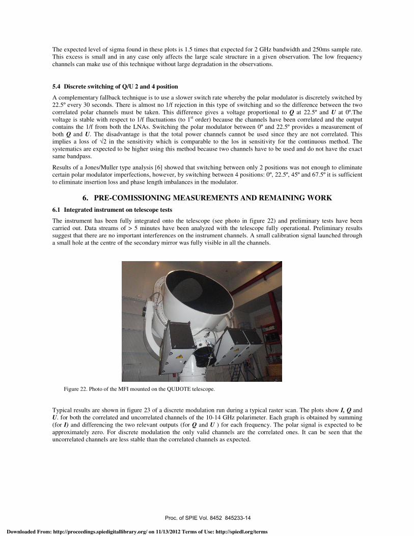
The instrument has been fully integrated onto the telescope (see photo in figure 22) and preliminary tests have been carried out. Data streams of > 5 minutes have been analyzed with the telescope fully operational. Preliminary results suggest that there are no important interferences on the instrument channels. A small calibration signal launched through a small hole at the centre of the secondary mirror was fully visible in all the channels.

Figure 22. Photo of the MFI mounted on the QUIJOTE telescope.

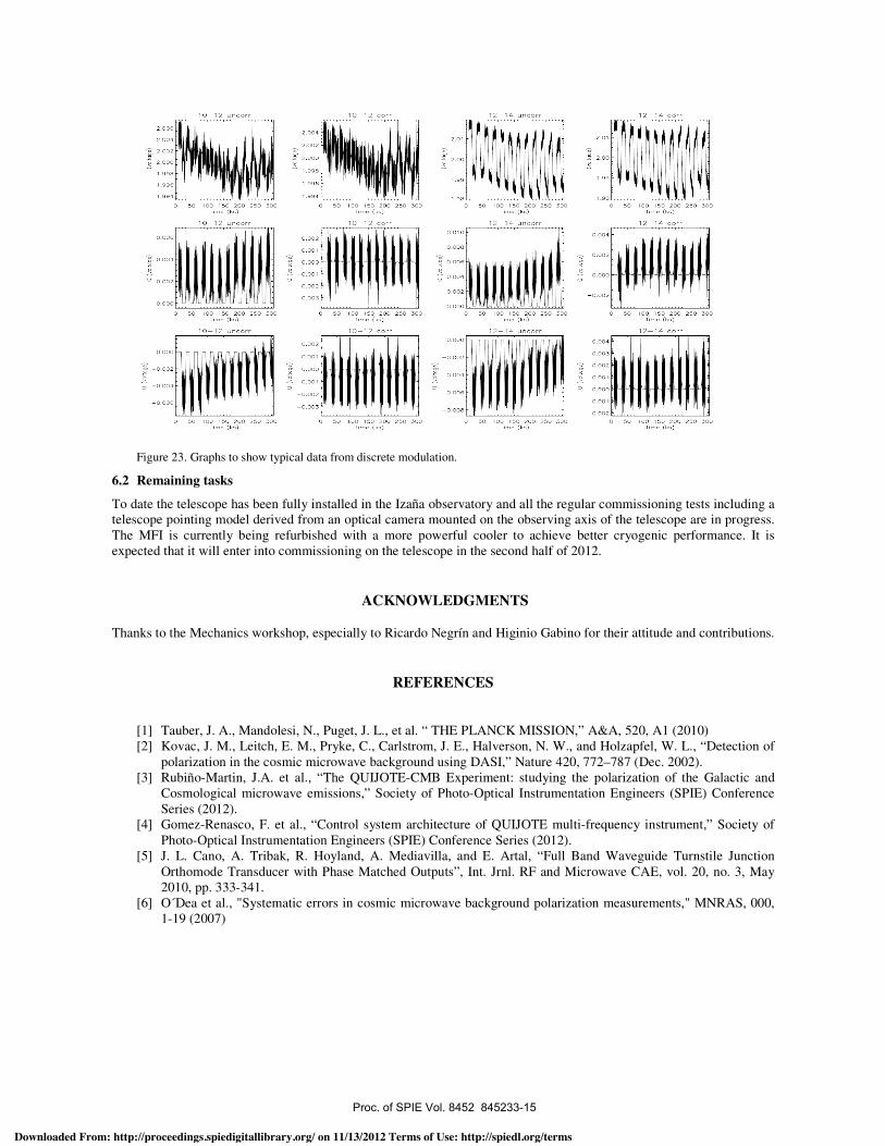
Typical results are shown in figure 23 of a discrete modulation run during a typical raster scan. The plots show I, Q and U. for both the correlated and uncorrelated channels of the 10-14 GHz polarimeter. Each graph is obtained by summing (for I) and differencing the two relevant outputs (for Q and U ) for each frequency. The polar signal is expected to be approximately zero. For discrete modulation the only valid channels are the correlated ones. It can be seen that the uncorrelated channels are less stable than the correlated channels as expected.

A'65<)63)*A2B):6#<)CDEF))CDEFGG1JD


Ill

() 000 000 000 Oct aot 0S

1 I

Dot

'I

0000 tOO 0

00

66

000 0

to)

LILtJJAJ LJLI

00 0 Ct

00 000 oDD oct CDL 00

000

(oo) (So) 0tt. C OCZ 000 Oct OCt 00

-too Cc Dc

lI

I

cc 0

0000 CD00

L0O0 -

0000 L0O.O

966

0000 0000 0000

ilti I Itt

CL

0 000 000 Oct OOL DL

Figure 23. Graphs to show typical data from discrete modulation.

6.2 Remaining tasks

To date the telescope has been fully installed in the Izaña observatory and all the regular commissioning tests including a telescope pointing model derived from an optical camera mounted on the observing axis of the telescope are in progress. The MFI is currently being refurbished with a more powerful cooler to achieve better cryogenic performance. It is expected that it will enter into commissioning on the telescope in the second half of 2012.

ACKNOWLEDGMENTS

Thanks to the Mechanics workshop, especially to Ricardo Negrín and Higinio Gabino for their attitude and contributions.

REFERENCES

[1] Tauber, J. A., Mandolesi, N., Puget, J. L., et al. “ THE PLANCK MISSION,” A&A, 520, A1 (2010) [2] Kovac, J. M., Leitch, E. M., Pryke, C., Carlstrom, J. E., Halverson, N. W., and Holzapfel, W. L., “Detection of

polarization in the cosmic microwave background using DASI,” Nature 420, 772–787 (Dec. 2002). [3] Rubiño-Martin, J.A. et al., “The QUIJOTE-CMB Experiment: studying the polarization of the Galactic and

Cosmological microwave emissions,” Society of Photo-Optical Instrumentation Engineers (SPIE) Conference Series (2012).

[4] Gomez-Renasco, F. et al., “Control system architecture of QUIJOTE multi-frequency instrument,” Society of Photo-Optical Instrumentation Engineers (SPIE) Conference Series (2012).

[5] J. L. Cano, A. Tribak, R. Hoyland, A. Mediavilla, and E. Artal, “Full Band Waveguide Turnstile Junction Orthomode Transducer with Phase Matched Outputs”, Int. Jrnl. RF and Microwave CAE, vol. 20, no. 3, May 2010, pp. 333-341.

[6] O´Dea et al., "Systematic errors in cosmic microwave background polarization measurements," MNRAS, 000, 1-19 (2007)

A'65<)63)*A2B):6#<)CDEF))CDEFGG1JE


Documents

THE STATUS OF THE QUIJOTE MULTI-FREQUENCY INSTRUMENTdigital.csic.es/bitstream/10261/109140/1/The status of the QUIJOTE.pdf · Here we present the current status of the QUIJOTE multi-frequency