Embed Size (px)
Citation preview
The Statistics of Causal Inference in theSocial Sciences1
Political Science 236AStatistics 239A
Jasjeet S. Sekhon
UC Berkeley
October 29, 2014
1 c© Copyright 20141 / 765
Background
• We are concerned with causal inference in the socialsciences.
• We discuss the potential outcomes framework of causalinference in detail.
• This framework originates with Jerzy Neyman (1894-1981),the founder of the Berkeley Statistics Department.
• A key insight of the framework is that causal inference is amissing data problem.
• The framework applies regardless of the method used toestimate causal effects, whether it be quantitative orqualitative.
2 / 765
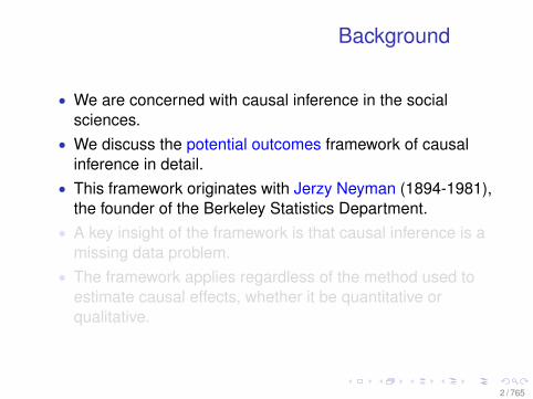
Background
• We are concerned with causal inference in the socialsciences.
• We discuss the potential outcomes framework of causalinference in detail.
• This framework originates with Jerzy Neyman (1894-1981),the founder of the Berkeley Statistics Department.
• A key insight of the framework is that causal inference is amissing data problem.
• The framework applies regardless of the method used toestimate causal effects, whether it be quantitative orqualitative.
3 / 765

The Problem
• Many of the great minds of the 18th and 19th centuriescontributed to the development of social statistics: DeMoivre, several Bernoullis, Gauss, Laplace, Quetelet,Galton, Pearson, and Yule.
• They searched for a method of statistical calculus thatwould do for social studies what Leibniz’s and Newton’scalculus did for physics.
• It quickly came apparent this is would be most difficult.• For example: deficits crowding out money versus
chemotherapy
4 / 765

The Problem
• Many of the great minds of the 18th and 19th centuriescontributed to the development of social statistics: DeMoivre, several Bernoullis, Gauss, Laplace, Quetelet,Galton, Pearson, and Yule.
• They searched for a method of statistical calculus thatwould do for social studies what Leibniz’s and Newton’scalculus did for physics.
• It quickly came apparent this is would be most difficult.• For example: deficits crowding out money versus
chemotherapy
5 / 765

The Experimental Model
• In the early 20th Century, Sir Ronald Fisher (1890-1962)helped to establish randomization as the “reasoned basisfor inference” (Fisher, 1935)
• Randomization: method by which systematic sources ofbias are made random
• Permutation (Fisherian) Inference
6 / 765
The Experimental Model
• In the early 20th Century, Sir Ronald Fisher (1890-1962)helped to establish randomization as the “reasoned basisfor inference” (Fisher, 1935)
• Randomization: method by which systematic sources ofbias are made random
• Permutation (Fisherian) Inference
7 / 765

Historical Note: Charles SandersPeirce
• Charles Sanders Peirce (1839–1914) independently, andbefore Fisher, developed permutation inference andrandomized experiments
• He introduced terms “confidence” and “likelihood”• Work was not well known until later. Betrand Russell wrote
(1959): “Beyond doubt [...] he was one of the most originalminds of the later nineteenth century, and certainly thegreatest American thinker ever.”
• Karl Popper (1972): “[He is] one of the greatestphilosophers of all times”
8 / 765

Historical Note: Charles SandersPeirce
• Charles Sanders Peirce (1839–1914) independently, andbefore Fisher, developed permutation inference andrandomized experiments
• He introduced terms “confidence” and “likelihood”• Work was not well known until later. Betrand Russell wrote
(1959): “Beyond doubt [...] he was one of the most originalminds of the later nineteenth century, and certainly thegreatest American thinker ever.”
• Karl Popper (1972): “[He is] one of the greatestphilosophers of all times”
9 / 765
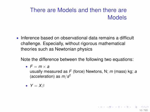
There are Models and then there areModels
• Inference based on observational data remains a difficultchallenge. Especially, without rigorous mathematicaltheories such as Newtonian physics
Note the difference between the following two equations:• F = m × a
usually measured as F (force) Newtons, N; m (mass) kg; a(acceleration) as m/s2
• Y = Xβ
10 / 765
Regression is Evil
• It was hoped that statistical inference through the use ofmultiple regression would be able to provide to the socialscientist what experiments and rigorous mathematicaltheories provide, respectively, to the micro-biologist andastronomer.
• OLS has unfortunately become a black box which peoplethink solves hard problems it actually doesn’t solve. It is inthis sense Evil.
• Let’s consider a simple sample to test intuition
11 / 765
Regression is Evil
• It was hoped that statistical inference through the use ofmultiple regression would be able to provide to the socialscientist what experiments and rigorous mathematicaltheories provide, respectively, to the micro-biologist andastronomer.
• OLS has unfortunately become a black box which peoplethink solves hard problems it actually doesn’t solve. It is inthis sense Evil.
• Let’s consider a simple sample to test intuition
12 / 765
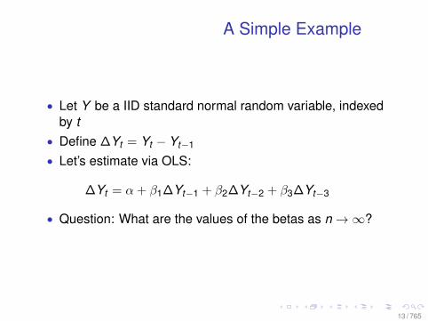
A Simple Example
• Let Y be a IID standard normal random variable, indexedby t
• Define ∆Yt = Yt − Yt−1
• Let’s estimate via OLS:
∆Yt = α + β1∆Yt−1 + β2∆Yt−2 + β3∆Yt−3
• Question: What are the values of the betas as n→∞?
13 / 765

A Simple Example II
• What about for:
∆Yt = α + β1∆Yt−1 + β2∆Yt−2 + · · ·+ βk ∆Yt−k
?
14 / 765
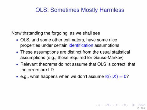
OLS: Sometimes Mostly Harmless
Notwithstanding the forgoing, as we shall see• OLS, and some other estimators, have some nice
properties under certain identification assumptions• These assumptions are distinct from the usual statistical
assumptions (e.g., those required for Gauss-Markov)• Relevant theorems do not assume that OLS is correct, that
the errors are IID.• e.g., what happens when we don’t assume E(ε|X ) = 0?
15 / 765

Early and Influential Methods
• John Stuart Mill (in his A System of Logic) devised a set offive methods (or canons) of inference.
• They were outlined in Book III, Chapter 8 of his book.• Unfortunately, people rarely read the very next chapter
entitled “Of Plurality of Causes: and of the Intermixture ofEffects.”
16 / 765
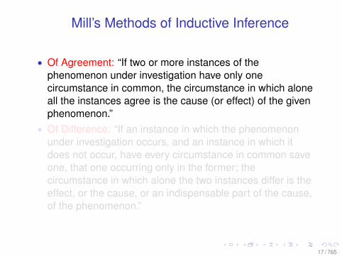
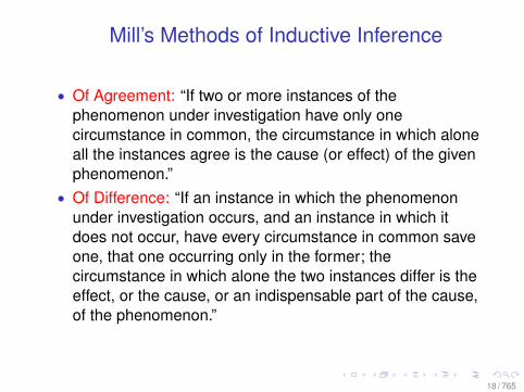
Mill’s Methods of Inductive Inference
• Of Agreement: “If two or more instances of thephenomenon under investigation have only onecircumstance in common, the circumstance in which aloneall the instances agree is the cause (or effect) of the givenphenomenon.”
• Of Difference: “If an instance in which the phenomenonunder investigation occurs, and an instance in which itdoes not occur, have every circumstance in common saveone, that one occurring only in the former; thecircumstance in which alone the two instances differ is theeffect, or the cause, or an indispensable part of the cause,of the phenomenon.”
17 / 765
Mill’s Methods of Inductive Inference
• Of Agreement: “If two or more instances of thephenomenon under investigation have only onecircumstance in common, the circumstance in which aloneall the instances agree is the cause (or effect) of the givenphenomenon.”
• Of Difference: “If an instance in which the phenomenonunder investigation occurs, and an instance in which itdoes not occur, have every circumstance in common saveone, that one occurring only in the former; thecircumstance in which alone the two instances differ is theeffect, or the cause, or an indispensable part of the cause,of the phenomenon.”
18 / 765
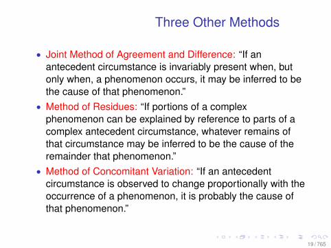
Three Other Methods
• Joint Method of Agreement and Difference: “If anantecedent circumstance is invariably present when, butonly when, a phenomenon occurs, it may be inferred to bethe cause of that phenomenon.”
• Method of Residues: “If portions of a complexphenomenon can be explained by reference to parts of acomplex antecedent circumstance, whatever remains ofthat circumstance may be inferred to be the cause of theremainder that phenomenon.”
• Method of Concomitant Variation: “If an antecedentcircumstance is observed to change proportionally with theoccurrence of a phenomenon, it is probably the cause ofthat phenomenon.”
19 / 765
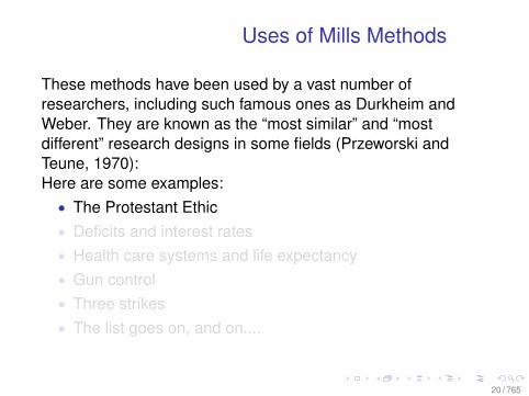
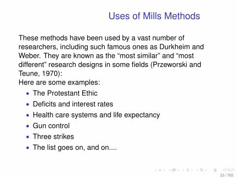
Uses of Mills Methods
These methods have been used by a vast number ofresearchers, including such famous ones as Durkheim andWeber. They are known as the “most similar” and “mostdifferent” research designs in some fields (Przeworski andTeune, 1970):Here are some examples:• The Protestant Ethic• Deficits and interest rates• Health care systems and life expectancy• Gun control• Three strikes• The list goes on, and on....
20 / 765
Uses of Mills Methods
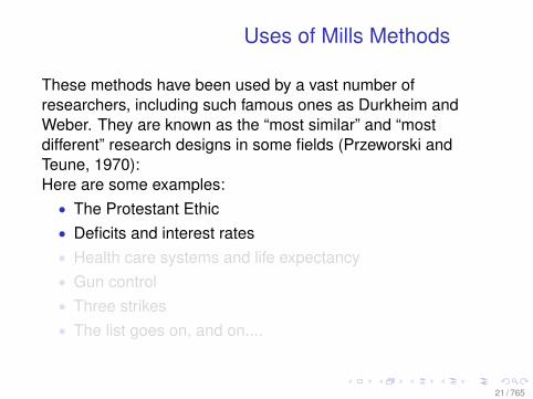
These methods have been used by a vast number ofresearchers, including such famous ones as Durkheim andWeber. They are known as the “most similar” and “mostdifferent” research designs in some fields (Przeworski andTeune, 1970):Here are some examples:• The Protestant Ethic• Deficits and interest rates• Health care systems and life expectancy• Gun control• Three strikes• The list goes on, and on....
21 / 765
Uses of Mills Methods
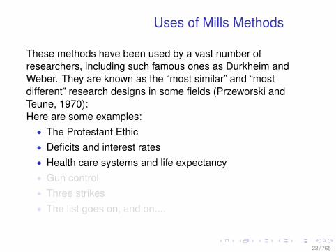
These methods have been used by a vast number ofresearchers, including such famous ones as Durkheim andWeber. They are known as the “most similar” and “mostdifferent” research designs in some fields (Przeworski andTeune, 1970):Here are some examples:• The Protestant Ethic• Deficits and interest rates• Health care systems and life expectancy• Gun control• Three strikes• The list goes on, and on....
22 / 765
Uses of Mills Methods
These methods have been used by a vast number ofresearchers, including such famous ones as Durkheim andWeber. They are known as the “most similar” and “mostdifferent” research designs in some fields (Przeworski andTeune, 1970):Here are some examples:• The Protestant Ethic• Deficits and interest rates• Health care systems and life expectancy• Gun control• Three strikes• The list goes on, and on....
23 / 765
Uses of Mills Methods
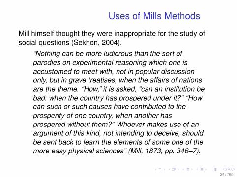
Mill himself thought they were inappropriate for the study ofsocial questions (Sekhon, 2004).
“Nothing can be more ludicrous than the sort ofparodies on experimental reasoning which one isaccustomed to meet with, not in popular discussiononly, but in grave treatises, when the affairs of nationsare the theme. “How,” it is asked, “can an institution bebad, when the country has prospered under it?” “Howcan such or such causes have contributed to theprosperity of one country, when another hasprospered without them?” Whoever makes use of anargument of this kind, not intending to deceive, shouldbe sent back to learn the elements of some one of themore easy physical sciences” (Mill, 1873, pp. 346–7).
24 / 765

Basic Statistical Inference
Let’s look at an example Mill himself brought up:
“In England, westerly winds blow during about twiceas great a portion of the year as easterly. If, therefore,it rains only twice as often with a westerly as with aneasterly wind, we have no reason to infer that any lawof nature is concerned in the coincidence. If it rainsmore than twice as often, we may be sure that somelaw is concerned; either there is some cause in naturewhich, in this climate, tends to produce both rain and awesterly wind, or a westerly wind has itself sometendency to produce rain.”
25 / 765
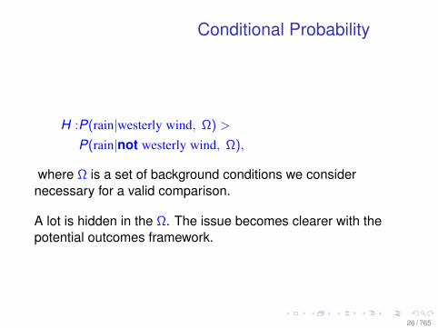
Conditional Probability
H :P(rain|westerly wind, Ω) >
P(rain|not westerly wind, Ω),
where Ω is a set of background conditions we considernecessary for a valid comparison.
A lot is hidden in the Ω. The issue becomes clearer with thepotential outcomes framework.
26 / 765
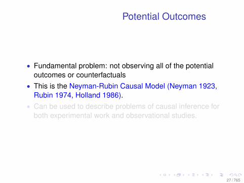
Potential Outcomes
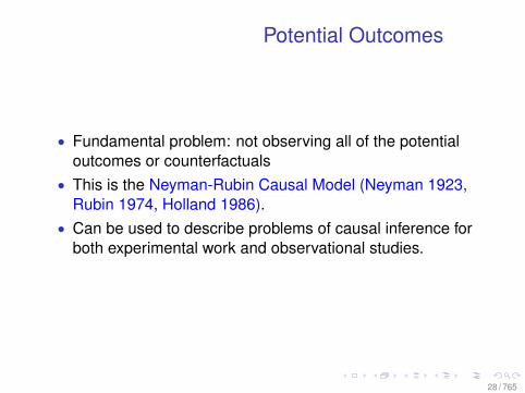
• Fundamental problem: not observing all of the potentialoutcomes or counterfactuals
• This is the Neyman-Rubin Causal Model (Neyman 1923,Rubin 1974, Holland 1986).
• Can be used to describe problems of causal inference forboth experimental work and observational studies.
27 / 765
Potential Outcomes
• Fundamental problem: not observing all of the potentialoutcomes or counterfactuals
• This is the Neyman-Rubin Causal Model (Neyman 1923,Rubin 1974, Holland 1986).
• Can be used to describe problems of causal inference forboth experimental work and observational studies.
28 / 765
Observational Study
An observational study concerns• cause-and-effect relationships• treatments, interventions or policies and• the effects they cause
The design stage of estimating the causal effect for treatment Tis common for all Y .
29 / 765
Observational Study
An observational study concerns• cause-and-effect relationships• treatments, interventions or policies and• the effects they cause
The design stage of estimating the causal effect for treatment Tis common for all Y .
30 / 765
A Thought Experiment
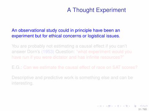
An observational study could in principle have been anexperiment but for ethical concerns or logistical issues.
You are probably not estimating a causal effect if you can’tanswer Dorn’s (1953) Question: “what experiment would youhave run if you were dictator and has infinite resources?”
E.G.: Can we estimate the causal effect of race on SAT scores?
Descriptive and predictive work is something else and can beinteresting.
31 / 765
A Thought Experiment
An observational study could in principle have been anexperiment but for ethical concerns or logistical issues.
You are probably not estimating a causal effect if you can’tanswer Dorn’s (1953) Question: “what experiment would youhave run if you were dictator and has infinite resources?”
E.G.: Can we estimate the causal effect of race on SAT scores?
Descriptive and predictive work is something else and can beinteresting.
32 / 765
A Thought Experiment
An observational study could in principle have been anexperiment but for ethical concerns or logistical issues.
You are probably not estimating a causal effect if you can’tanswer Dorn’s (1953) Question: “what experiment would youhave run if you were dictator and has infinite resources?”
E.G.: Can we estimate the causal effect of race on SAT scores?
Descriptive and predictive work is something else and can beinteresting.
33 / 765
A Thought Experiment
An observational study could in principle have been anexperiment but for ethical concerns or logistical issues.
You are probably not estimating a causal effect if you can’tanswer Dorn’s (1953) Question: “what experiment would youhave run if you were dictator and has infinite resources?”
E.G.: Can we estimate the causal effect of race on SAT scores?
Descriptive and predictive work is something else and can beinteresting.
34 / 765

10/4/13 11:24 PMford - Google Search
Page 1 of 2https://www.google.com/#q=ford
About 868,000,000 results (0.30 seconds)
Crosscut
ford near Berkeley, CA
See results for ford on a map »
News for ford
Ads related to ford
Ford.com - Ford Focus Official Site www.ford.com/FocusBe Everywhere @ Once w/ Up to 40MPG Ford Focus. Learn More @ Ford.com.
Build and PriceBuild & Price the 2014 Ford Focus.A Small Car That's Big On Features!
Photo GallerySee Interior & Exterior Photosof the 2014 Focus @ Ford.com.
2013 Toyota Camry - BuyAToyota.com www.buyatoyota.com/Camry0% for 60 mos PLUS $1,000 Trade-in Cash on a new Camry. Learn more.
Ford – New Cars, Trucks, SUVs, Hybrids & Crossovers | Ford Vehicleswww.ford.com/The Official Ford Site to research, learn and shop for all new Ford Vehicles. Viewphotos, videos, specs, compare competitors, build and price, search inventory ...All Vehicles - 2013 F-150 - Mustang - 2014 Ford Focus77,507 people +1'd this
Ford Dealership Charleston, North Charleston ... - Moncks Cornerberkeleyford.net/ Visit the Official Site of Berkeley Ford, Selling Ford in Moncks Corner, SC and ServingCharleston. 1511 Highway 52, Moncks Corner, SC 29461.
Used Vehicle For Sale | Berkeley Ford Serving ... - Moncks Cornerberkeleyford.net/Charleston/For-Sale/Used/Shop now for Used Cars For Sale in Charleston . See the available vehicles to buy now.
Albany Ford Subaruwww.albanyfordsubaru.com3.9 6 Google reviews
718 San Pablo AveAlbany(510) 528-1244
East Bay Ford Truck Centerwww.eastbaytruckcenter.com2 Google reviews
333 Filbert StOakland(510) 272-4400
Albany Ford Subaru | New Ford, Subaru dealership in Albany, CA ...www.albanyfordsubaru.com/Albany, CA New, Albany Ford Subaru sells and services Ford, Subaru vehicles in thegreater Albany area.
New Vehicle For Sale | Berkeley Ford Serving ... - Moncks Cornerberkeleyford.net/Charleston/For-Sale/New/Shop now for New Cars For Sale in Charleston . See the available vehicles to buy now.
Ford's Mulally dispels Microsoft CEO rumorsUSA TODAY - by Mike Snider - 2 days agoATHENS, Ga. – Despite resurfaced rumors that he is on the very short listto replace outgoing CEO Steve Ballmer at Microsoft, Ford CEO Alan ...
Ford's Mulally brushes off Microsoft CEO chatterCNET - 3 days ago
Find Ford Dealers in Berkeley, California - Edmunds.comwww.edmunds.com › Car Dealers › Ford › California › Alameda CountyFind Ford Dealers in Berkeley, California. The process of buying a new Ford car or truck
Ford MotorCompany2,620,994 followers on Google+
Ford Motor Company is an Americanmultinational automaker headquartered inDearborn, Michigan, a suburb of Detroit. It wasfounded by Henry Ford and incorporated onJune 16, 1903. Wikipedia
CEO: Alan Mulally
Headquarters: Dearborn, MI
Founder: Henry Ford
Founded: June 16, 1903
Awards: Car and Driver 10Best, Motor Trend Car of the Year, More
#FiestaST Duel - Two racing drivers battle it out.Johnny Herbert vs Dan Cammish - Formula Ford &Fiesta ST ... and the winner is?
ToyotaMotorCorporation
VolkswagenPassengerCars
HondaMotorCompany...
Dodge Mazda
Recent posts
Oct 1, 2013
People also search for
Feedback / More info
Map for ford
Web Images Maps Shopping News Search toolsMore
SIGN INford
35 / 765

10/4/13 11:24 PMebay - Google Search
Page 1 of 2https://www.google.com/#q=ebay
About 1,730,000,000 results (0.19 seconds)
More results from ebay.com »
News for ebay
In-depth articles
eBay: Electronics, Cars, Fashion, Collectibles, Coupons and More ...www.ebay.com/Buy and sell electronics, cars, fashion apparel, collectibles, sporting goods, digitalcameras, baby items, coupons, and everything else on eBay, the world's ...
MotorsCars Trucks - Parts & Accessories -Collector Cars - Motorcycles
Cars TrucksSalvage - Truck - Rat rod - eBayMotors - Project - No Reserve
WomenTops & Blouses - Coats & Jackets -Swimwear - Shoes - Sweaters
MenCasual Shirts - Jeans - Coats &Jackets - Shorts - Dress Shirts
Daily DealsDeals are updated daily, so checkback for the deepest discounts ...
Cell Phone, AccessoriesCell Phones & Accessories. CellPhones & Smartphones · Cell ...
How the eBay of Illegal Drugs Came UndoneNew Yorker (blog) - 12 hours agoIf the F.B.I.'s allegations are true, Silk Road was undone by the zeal andcarelessness of its owner, Ross William Ulbricht.
How to Get the Most Money Out of Your eBay AuctionsTIME - 20 hours agoSilk Road Accused Denies Running 'Drugs Ebay'Sky News - 4 hours ago
Cars Trucks | eBaymotors.shop.ebay.com › BuyFord : Mustang. 1996 Ford Mustang SVT Cobra Coupe. Location: Franklin, MI. Watchthis item. Get fast shipping and excellent service when you buy from eBay ...You recently searched for ford.
Ford Mustang - eBay Motorshub.motors.ebay.com › eBay Motors › Collector CarsFord Mustang overview, descriptions of generations of Ford Mustangs, history,characteristics, pricing and specifications. Provided by eBay Motors.
eBay Classifieds (Kijiji) - Post & Search Free Local Classified Ads.www.ebayclassifieds.com/Use free eBay Classifieds (Kijiji) to buy & sell locally all over the United States.
eBay - Wikipedia, the free encyclopediaen.wikipedia.org/wiki/EBay eBay Inc. is an American multinational internet consumer-to-consumer corporation,headquartered in San Jose, California. It was founded in 1995, and became ...
eBay for iPad for iPad on the iTunes App Storehttps://itunes.apple.com/us/app/ebay-for-ipad/id364203371?mt=8
Rating: 4.5 - 18,295 votes - Free - iOSSep 17, 2013 - Description. The eBay for iPad app lets you sell, search, bid, buy,browse, and pay in an interface optimized for the iPad. With seamless ...
Behind eBay's ComebackThe New York Times - Jul 2012The Internet company's surprise earnings report was the result oftechnological innovation, a management overhaul and an embrace of newopportunities.
eBayCorporation
eBay Inc. is an American multinational internetconsumer-to-consumer corporation,headquartered in San Jose, California. Wikipedia
Customer service: 1 (866) 540-3229(Consumer)
Stock price: EBAY (NASDAQ) $55.58 +0.67 (+1.22%)Oct 4, 4:00 PM EDT - Disclaimer
Founder: Pierre Omidyar
Founded: September 3, 1995, Campbell, CA
Headquarters: San Jose, CA
CEO: John Donahoe
Amazon.c… UnitedStatesPostal Se...
CraigslistInc.
Yahoo! Apple
People also search for
Feedback / More info
Web Images Maps Shopping News Search toolsMore
SIGN INebay
36 / 765
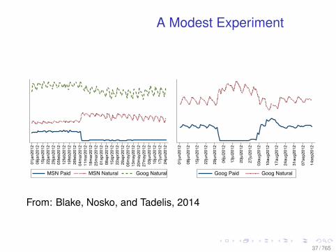
A Modest Experiment
Figure 2: Brand Keyword Click Substitution
01ja
n201
208
jan2
012
15ja
n201
222
jan2
012
29ja
n201
205
feb2
012
12fe
b201
219
feb2
012
26fe
b201
204
mar
2012
11m
ar20
1218
mar
2012
25m
ar20
1201
apr2
012
08ap
r201
215
apr2
012
22ap
r201
229
apr2
012
06m
ay20
1213
may
2012
20m
ay20
1227
may
2012
03ju
n201
210
jun2
012
17ju
n201
224
jun2
012
MSN Paid MSN Natural Goog Natural
(a) MSN Test
01ju
n201
2
08ju
n201
2
15ju
n201
2
22ju
n201
2
29ju
n201
2
06ju
l201
2
13ju
l201
2
20ju
l201
2
27ju
l201
2
03au
g201
2
10au
g201
2
17au
g201
2
24au
g201
2
31au
g201
2
07se
p201
2
14se
p201
2
Goog Paid Goog Natural
(b) Google Test
MSN and Google click trac is shown for two events where paid search was suspended (Left)
and suspended and resumed (Right).
To quantify this substitution, Table 1 shows estimates from a simple pre-post comparison
as well as a simple di↵erence-in-di↵erences across search platforms. In the pre-post analysis
we regress the log of total daily clicks from MSN to eBay on an indicator for whether days
were in the period with ads turned o↵. Column 1 shows the results which suggest that
click volume was only 5.6 percent lower in the period after advertising was suspended.
This approach lacks any reasonable control group. It is apparent from Figure 2a that
trac increases in daily volatility and begins to decline after the advertising is turned
o↵. Both of these can be attributed to the seasonal nature of e-commerce. We look to
another search platform which serves as a source for eBay trac, Google, as a control
group to account for seasonal factors. During the test period on MSN, eBay continued to
purchase brand keyword advertising on Google which can serve as a control group. With
this data, we calculate the impact of brand keyword advertising on total click trac. In
the di↵erence-in-di↵erences approach, we add observations of daily trac from Google
and Yahoo! and include in the specification search engine dummies and trends.15 The
variable of interest is thus the interaction between a dummy for the MSN platform and a
dummy for treatment (ad o↵) period. Column 2 of Table 1 show a much smaller impact
15The estimates presented include date fixed e↵ects and platform specific trends but the results arevery similar without these controls.
9
From: Blake, Nosko, and Tadelis, 2014
37 / 765
General Problems with ObservationalStudies
• Prediction accuracy is uninformative• No randomization, the “reasoned basis for inference”• Selection problems abound• Data/Model Mining—e.g., not like vision• Found data, usually retrospective
Note: it is far easier to estimate the effect of a cause than thecause of an effect. Why?
38 / 765
General Problems with ObservationalStudies
• Prediction accuracy is uninformative• No randomization, the “reasoned basis for inference”• Selection problems abound• Data/Model Mining—e.g., not like vision• Found data, usually retrospective
Note: it is far easier to estimate the effect of a cause than thecause of an effect. Why?
39 / 765
General Problems with ObservationalStudies
• Prediction accuracy is uninformative• No randomization, the “reasoned basis for inference”• Selection problems abound• Data/Model Mining—e.g., not like vision• Found data, usually retrospective
Note: it is far easier to estimate the effect of a cause than thecause of an effect. Why?
40 / 765
General Problems with ObservationalStudies
• Prediction accuracy is uninformative• No randomization, the “reasoned basis for inference”• Selection problems abound• Data/Model Mining—e.g., not like vision• Found data, usually retrospective
Note: it is far easier to estimate the effect of a cause than thecause of an effect. Why?
41 / 765
General Problems with ObservationalStudies
• Prediction accuracy is uninformative• No randomization, the “reasoned basis for inference”• Selection problems abound• Data/Model Mining—e.g., not like vision• Found data, usually retrospective
Note: it is far easier to estimate the effect of a cause than thecause of an effect. Why?
42 / 765
Difficult Example: Does InformationMatter?
• We want to estimate the effect on voting behavior of payingattention to an election campaign.
• Survey research is strikingly uniform regarding theignorance of the public (e.g., Berelson, Lazarsfeld, andMcPhee, 1954; Campbell et al., 1960; J. R. Zaller, 1992).
• Although the fact of public ignorance has not beenforcefully challenged, the meaning of this observation hasbeen (Sniderman, 1993).
• Can voters use information such as polls, interest groupendorsements and partisan labels to vote like their betterinformed compatriots (e.g., Lupia, 2004; McKelvey andOrdeshook, 1985a; McKelvey and Ordeshook, 1985b;McKelvey and Ordeshook, 1986)?
43 / 765
Difficult Example: Does InformationMatter?
• We want to estimate the effect on voting behavior of payingattention to an election campaign.
• Survey research is strikingly uniform regarding theignorance of the public (e.g., Berelson, Lazarsfeld, andMcPhee, 1954; Campbell et al., 1960; J. R. Zaller, 1992).
• Although the fact of public ignorance has not beenforcefully challenged, the meaning of this observation hasbeen (Sniderman, 1993).
• Can voters use information such as polls, interest groupendorsements and partisan labels to vote like their betterinformed compatriots (e.g., Lupia, 2004; McKelvey andOrdeshook, 1985a; McKelvey and Ordeshook, 1985b;McKelvey and Ordeshook, 1986)?
44 / 765
Difficult Example: Does InformationMatter?
• We want to estimate the effect on voting behavior of payingattention to an election campaign.
• Survey research is strikingly uniform regarding theignorance of the public (e.g., Berelson, Lazarsfeld, andMcPhee, 1954; Campbell et al., 1960; J. R. Zaller, 1992).
• Although the fact of public ignorance has not beenforcefully challenged, the meaning of this observation hasbeen (Sniderman, 1993).
• Can voters use information such as polls, interest groupendorsements and partisan labels to vote like their betterinformed compatriots (e.g., Lupia, 2004; McKelvey andOrdeshook, 1985a; McKelvey and Ordeshook, 1985b;McKelvey and Ordeshook, 1986)?
45 / 765
Difficult Example: Does InformationMatter?
• We want to estimate the effect on voting behavior of payingattention to an election campaign.
• Survey research is strikingly uniform regarding theignorance of the public (e.g., Berelson, Lazarsfeld, andMcPhee, 1954; Campbell et al., 1960; J. R. Zaller, 1992).
• Although the fact of public ignorance has not beenforcefully challenged, the meaning of this observation hasbeen (Sniderman, 1993).
• Can voters use information such as polls, interest groupendorsements and partisan labels to vote like their betterinformed compatriots (e.g., Lupia, 2004; McKelvey andOrdeshook, 1985a; McKelvey and Ordeshook, 1985b;McKelvey and Ordeshook, 1986)?
46 / 765
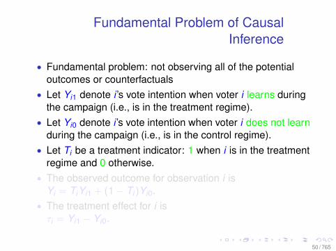
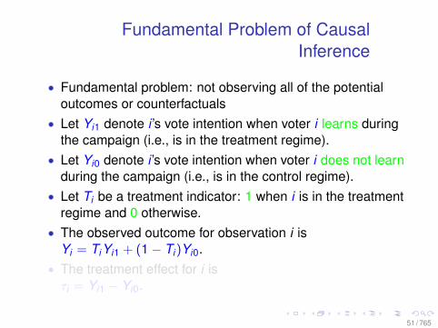
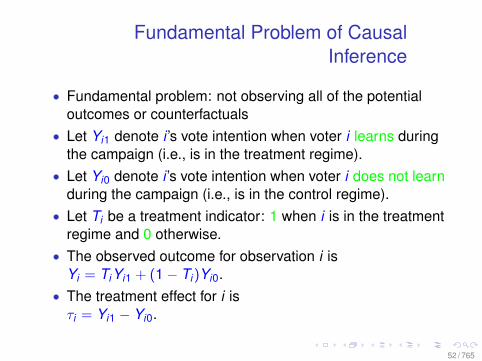
Fundamental Problem of CausalInference
• Fundamental problem: not observing all of the potentialoutcomes or counterfactuals
• Let Yi1 denote i ’s vote intention when voter i learns duringthe campaign (i.e., is in the treatment regime).
• Let Yi0 denote i ’s vote intention when voter i does not learnduring the campaign (i.e., is in the control regime).
• Let Ti be a treatment indicator: 1 when i is in the treatmentregime and 0 otherwise.
• The observed outcome for observation i isYi = TiYi1 + (1− Ti)Yi0.
• The treatment effect for i isτi = Yi1 − Yi0.
47 / 765
Fundamental Problem of CausalInference
• Fundamental problem: not observing all of the potentialoutcomes or counterfactuals
• Let Yi1 denote i ’s vote intention when voter i learns duringthe campaign (i.e., is in the treatment regime).
• Let Yi0 denote i ’s vote intention when voter i does not learnduring the campaign (i.e., is in the control regime).
• Let Ti be a treatment indicator: 1 when i is in the treatmentregime and 0 otherwise.
• The observed outcome for observation i isYi = TiYi1 + (1− Ti)Yi0.
• The treatment effect for i isτi = Yi1 − Yi0.
48 / 765
Fundamental Problem of CausalInference
• Fundamental problem: not observing all of the potentialoutcomes or counterfactuals
• Let Yi1 denote i ’s vote intention when voter i learns duringthe campaign (i.e., is in the treatment regime).
• Let Yi0 denote i ’s vote intention when voter i does not learnduring the campaign (i.e., is in the control regime).
• Let Ti be a treatment indicator: 1 when i is in the treatmentregime and 0 otherwise.
• The observed outcome for observation i isYi = TiYi1 + (1− Ti)Yi0.
• The treatment effect for i isτi = Yi1 − Yi0.
49 / 765
Fundamental Problem of CausalInference
• Fundamental problem: not observing all of the potentialoutcomes or counterfactuals
• Let Yi1 denote i ’s vote intention when voter i learns duringthe campaign (i.e., is in the treatment regime).
• Let Yi0 denote i ’s vote intention when voter i does not learnduring the campaign (i.e., is in the control regime).
• Let Ti be a treatment indicator: 1 when i is in the treatmentregime and 0 otherwise.
• The observed outcome for observation i isYi = TiYi1 + (1− Ti)Yi0.
• The treatment effect for i isτi = Yi1 − Yi0.
50 / 765
Fundamental Problem of CausalInference
• Fundamental problem: not observing all of the potentialoutcomes or counterfactuals
• Let Yi1 denote i ’s vote intention when voter i learns duringthe campaign (i.e., is in the treatment regime).
• Let Yi0 denote i ’s vote intention when voter i does not learnduring the campaign (i.e., is in the control regime).
• Let Ti be a treatment indicator: 1 when i is in the treatmentregime and 0 otherwise.
• The observed outcome for observation i isYi = TiYi1 + (1− Ti)Yi0.
• The treatment effect for i isτi = Yi1 − Yi0.
51 / 765
Fundamental Problem of CausalInference
• Fundamental problem: not observing all of the potentialoutcomes or counterfactuals
• Let Yi1 denote i ’s vote intention when voter i learns duringthe campaign (i.e., is in the treatment regime).
• Let Yi0 denote i ’s vote intention when voter i does not learnduring the campaign (i.e., is in the control regime).
• Let Ti be a treatment indicator: 1 when i is in the treatmentregime and 0 otherwise.
• The observed outcome for observation i isYi = TiYi1 + (1− Ti)Yi0.
• The treatment effect for i isτi = Yi1 − Yi0.
52 / 765
Probability Model I: RepeatedSampling
• Assume that Yi(t) is a simple random sample from aninfinite population, were Y is the outcome of unit i undertreatment condition t .
• Assume the treat T is randomly assigned following either:• Bernoulli assignment to each i• Complete randomization
53 / 765
Probability Model II: Fixed Population
• Assume that Yi(t) is a fixed population
• Assume the treat T is randomly assigned following either:• Bernoulli assignment to each i• Complete randomization
54 / 765
Assignment Mechanism, ClassicalExperiment
• individualistic• probabilistic• unconfounded: given covariates, not be dependent on any
potential outcomes
55 / 765
Notation
Let:• N denote the number of units [in the sample], indexed by i• number of control units: Nc =
∑Ni=1(1− Ti); treated units:
Nt =∑N
i=1(Ti), Nc + Nt = N• Xi is a vector of K covariates, where X is a N × K matrix• Y (0) and Y (1) denote N-component vectors
56 / 765
Notation
• Let T be the N-dimensional vector with elements Ti ∈ 0,1with positive probability
• Let all possible values be T = 0,1N , with cardinality 2N
• 0,1N denotes the set of all N vectors with all elementsequal to 0 or 1
• Let the subset of values for T with positive probability bedenoted by T+
57 / 765
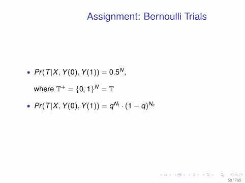
Assignment: Bernoulli Trials
• Pr(T |X ,Y (0),Y (1)) = 0.5N ,
where T+ = 0,1N = T
• Pr(T |X ,Y (0),Y (1)) = qNt · (1− q)Nc
58 / 765
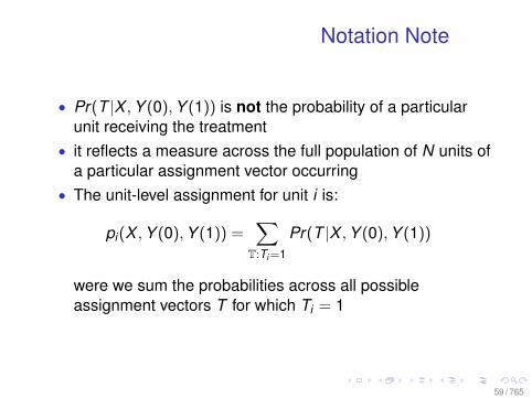
Notation Note
• Pr(T |X ,Y (0),Y (1)) is not the probability of a particularunit receiving the treatment
• it reflects a measure across the full population of N units ofa particular assignment vector occurring
• The unit-level assignment for unit i is:
pi(X ,Y (0),Y (1)) =∑
T:Ti =1
Pr(T |X ,Y (0),Y (1))
were we sum the probabilities across all possibleassignment vectors T for which Ti = 1
59 / 765
Assignment: Complete Randomization
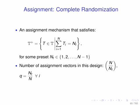
• An assignment mechanism that satisfies:
T+ =
T ∈ T
∣∣∣∣∣N∑
i=1
Ti = Nt
,
for some preset Nt ∈ 1,2, . . . ,N − 1
• Number of assignment vectors in this design:(
NNt
),
q =Nt
N∀ i
60 / 765
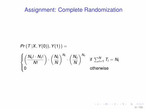
Assignment: Complete Randomization
Pr (T |X ,Y (0)),Y (1)) =(
Nc! · N t !
N!
)·(
Nt
N
)Nt
·(
Nc
N
)Nc
if∑N
i=1 Ti = Nt
0 otherwise
61 / 765
Experimental Data
• Under classic randomization, the inference problem isstraightforward because: T ⊥⊥ (Y (1),Y (0))
• Observations in the treatment and control groups are notexactly alike, but they are comparable—i.e., they areexchangeable
• With exchangeability plus noninterference between units,for j = 0,1 we have:
E(Y (j)|T = 1) = E(Y (j)|T = 0)
62 / 765
Experimental Data
• Under classic randomization, the inference problem isstraightforward because: T ⊥⊥ (Y (1),Y (0))
• Observations in the treatment and control groups are notexactly alike, but they are comparable—i.e., they areexchangeable
• With exchangeability plus noninterference between units,for j = 0,1 we have:
E(Y (j)|T = 1) = E(Y (j)|T = 0)
63 / 765
Experimental Data
• Under classic randomization, the inference problem isstraightforward because: T ⊥⊥ (Y (1),Y (0))
• Observations in the treatment and control groups are notexactly alike, but they are comparable—i.e., they areexchangeable
• With exchangeability plus noninterference between units,for j = 0,1 we have:
E(Y (j)|T = 1) = E(Y (j)|T = 0)
64 / 765
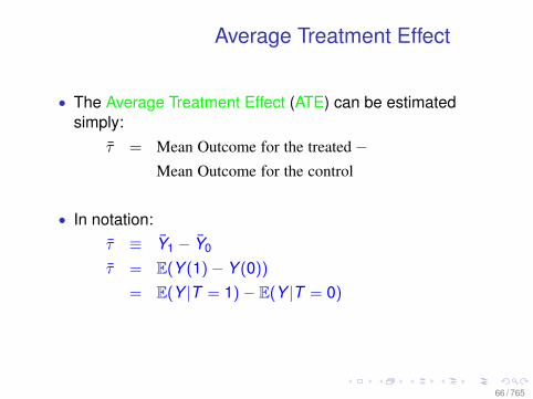
Average Treatment Effect
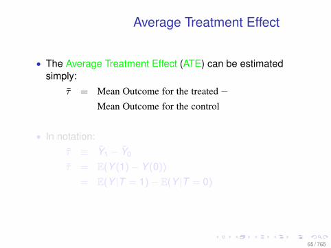
• The Average Treatment Effect (ATE) can be estimatedsimply:
τ = Mean Outcome for the treated−Mean Outcome for the control
• In notation:τ ≡ Y1 − Y0
τ = E(Y (1)− Y (0))
= E(Y |T = 1)− E(Y |T = 0)
65 / 765
Average Treatment Effect
• The Average Treatment Effect (ATE) can be estimatedsimply:
τ = Mean Outcome for the treated−Mean Outcome for the control
• In notation:τ ≡ Y1 − Y0
τ = E(Y (1)− Y (0))
= E(Y |T = 1)− E(Y |T = 0)
66 / 765
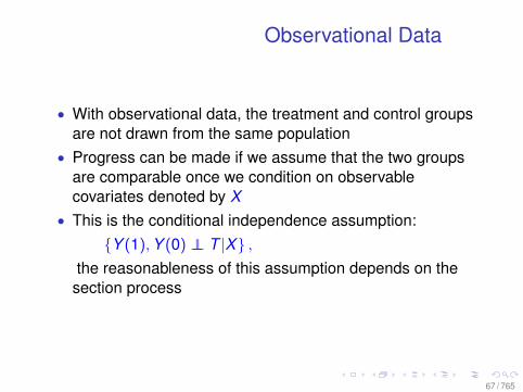
Observational Data
• With observational data, the treatment and control groupsare not drawn from the same population
• Progress can be made if we assume that the two groupsare comparable once we condition on observablecovariates denoted by X
• This is the conditional independence assumption:Y (1),Y (0) ⊥⊥ T |X ,
the reasonableness of this assumption depends on thesection process
67 / 765
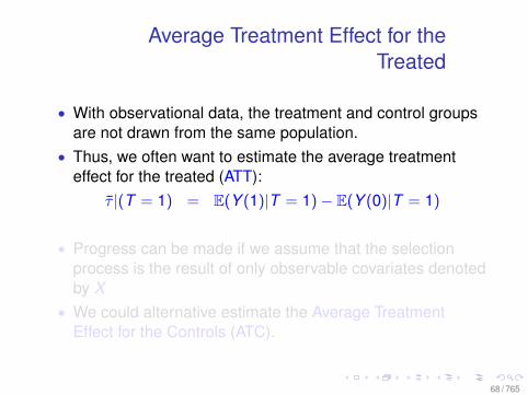
Average Treatment Effect for theTreated
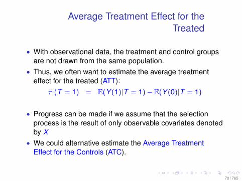
• With observational data, the treatment and control groupsare not drawn from the same population.
• Thus, we often want to estimate the average treatmenteffect for the treated (ATT):
τ |(T = 1) = E(Y (1)|T = 1)− E(Y (0)|T = 1)
• Progress can be made if we assume that the selectionprocess is the result of only observable covariates denotedby X
• We could alternative estimate the Average TreatmentEffect for the Controls (ATC).
68 / 765
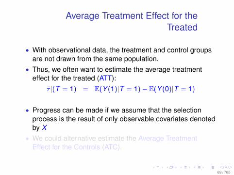
Average Treatment Effect for theTreated
• With observational data, the treatment and control groupsare not drawn from the same population.
• Thus, we often want to estimate the average treatmenteffect for the treated (ATT):
τ |(T = 1) = E(Y (1)|T = 1)− E(Y (0)|T = 1)
• Progress can be made if we assume that the selectionprocess is the result of only observable covariates denotedby X
• We could alternative estimate the Average TreatmentEffect for the Controls (ATC).
69 / 765
Average Treatment Effect for theTreated
• With observational data, the treatment and control groupsare not drawn from the same population.
• Thus, we often want to estimate the average treatmenteffect for the treated (ATT):
τ |(T = 1) = E(Y (1)|T = 1)− E(Y (0)|T = 1)
• Progress can be made if we assume that the selectionprocess is the result of only observable covariates denotedby X
• We could alternative estimate the Average TreatmentEffect for the Controls (ATC).
70 / 765
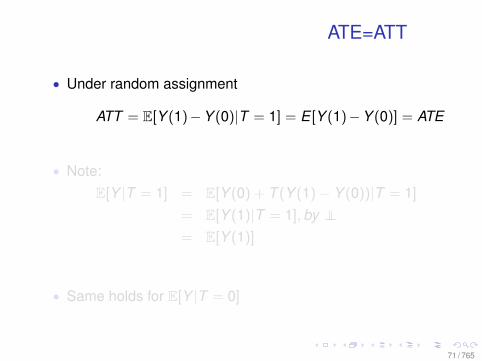
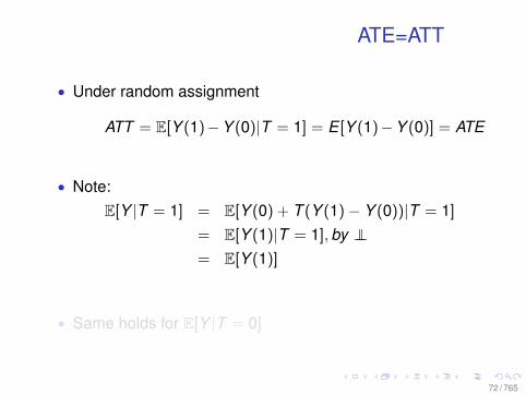
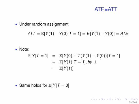
ATE=ATT
• Under random assignment
ATT = E[Y (1)−Y (0)|T = 1] = E [Y (1)−Y (0)] = ATE
• Note:E[Y |T = 1] = E[Y (0) + T (Y (1)− Y (0))|T = 1]
= E[Y (1)|T = 1],by ⊥⊥= E[Y (1)]
• Same holds for E[Y |T = 0]
71 / 765
ATE=ATT
• Under random assignment
ATT = E[Y (1)−Y (0)|T = 1] = E [Y (1)−Y (0)] = ATE
• Note:E[Y |T = 1] = E[Y (0) + T (Y (1)− Y (0))|T = 1]
= E[Y (1)|T = 1],by ⊥⊥= E[Y (1)]
• Same holds for E[Y |T = 0]
72 / 765
ATE=ATT
• Under random assignment
ATT = E[Y (1)−Y (0)|T = 1] = E [Y (1)−Y (0)] = ATE
• Note:E[Y |T = 1] = E[Y (0) + T (Y (1)− Y (0))|T = 1]
= E[Y (1)|T = 1],by ⊥⊥= E[Y (1)]
• Same holds for E[Y |T = 0]
73 / 765
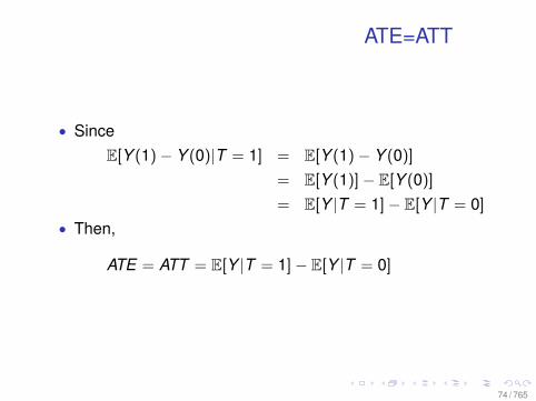
ATE=ATT
• SinceE[Y (1)− Y (0)|T = 1] = E[Y (1)− Y (0)]
= E[Y (1)]− E[Y (0)]
= E[Y |T = 1]− E[Y |T = 0]
• Then,
ATE = ATT = E[Y |T = 1]− E[Y |T = 0]
74 / 765
Review and Details
• More details on ATE, ATT, and potential outcomes: [LINK]
• Some review of probability: [LINK]
75 / 765
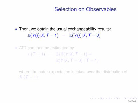
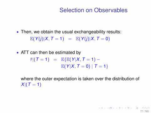
Selection on Observables
• Then, we obtain the usual exchangeability results:E(Y (j)|X ,T = 1) = E(Y (j)|X ,T = 0)
• ATT can then be estimated byτ |(T = 1) = EE(Y |X ,T = 1)−
E(Y |X ,T = 0) | T = 1
where the outer expectation is taken over the distribution ofX |(T = 1)
76 / 765
Selection on Observables
• Then, we obtain the usual exchangeability results:E(Y (j)|X ,T = 1) = E(Y (j)|X ,T = 0)
• ATT can then be estimated byτ |(T = 1) = EE(Y |X ,T = 1)−
E(Y |X ,T = 0) | T = 1
where the outer expectation is taken over the distribution ofX |(T = 1)
77 / 765
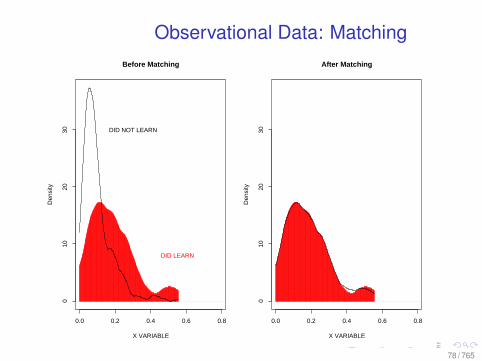
Observational Data: Matching
0.0 0.2 0.4 0.6 0.8
010
2030
Before Matching
X VARIABLE
Den
sity
DID NOT LEARN
DID LEARN
0.0 0.2 0.4 0.6 0.8
010
2030
After Matching
X VARIABLE
Den
sity
78 / 765
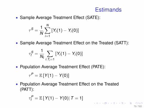
Estimands• Sample Average Treatment Effect (SATE):
τS =1N
N∑i=1
[Yi(1)− Yi(0)]
• Sample Average Treatment Effect on the Treated (SATT):
τSt =
1Nt
∑i:Ti =1
[Yi(1)− Yi(0)]
• Population Average Treatment Effect (PATE):
τP = E [Y (1)− Y (0)]
• Population Average Treatment Effect on the Treated(PATT):
τPt = E [Y (1)− Y (0)|T = 1]
79 / 765
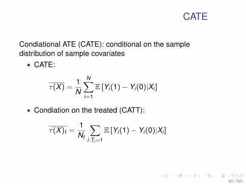
CATE
Condiational ATE (CATE): conditional on the sampledistribution of sample covariates• CATE:
τ(X ) =1N
N∑i=1
E [Yi(1)− Yi(0)|Xi ]
• Condiation on the treated (CATT):
τ(X )t =1Nt
∑i:Ti =1
E [Yi(1)− Yi(0)|Xi ]
80 / 765
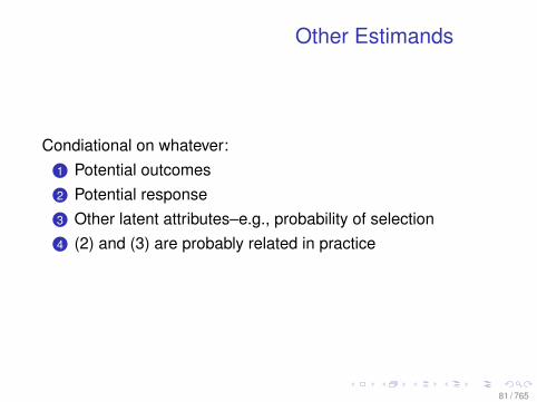
Other Estimands
Condiational on whatever:1 Potential outcomes2 Potential response3 Other latent attributes–e.g., probability of selection4 (2) and (3) are probably related in practice
81 / 765
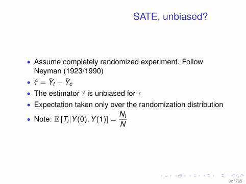
SATE, unbiased?
• Assume completely randomized experiment. FollowNeyman (1923/1990)
• τ = Yt − Yc
• The estimator τ is unbiased for τ• Expectation taken only over the randomization distribution
• Note: E [Ti |Y (0),Y (1)] =Nt
N
82 / 765
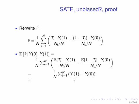
SATE, unbiased?, proof
• Rerwrite τ :
τ =1N
N∑i=1
(Ti · Yi(1)
Nt/N− (1− Ti) · Yi(0)
Nc/N
)• E [ τ |Y (0),Y (1)] =
1N∑N
i=1
(E[Ti ] · Yi(1)
Nt/N− E[1− Ti ] · Yi(0)
Nc/N
)=
1N∑N
i=1 (Yi(1)− Yi(0))
= τ
83 / 765
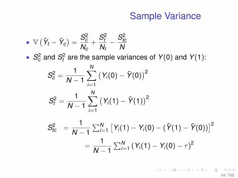
Sample Variance
• V(Yt − Yc
)=
S2c
Nc+
S2t
Nt− S2
tcN
• S2c and S2
t are the sample variances of Y (0) and Y (1):
S2c =
1N − 1
N∑i=1
(Yi(0)− Y (0)
)2
S2t =
1N − 1
N∑i=1
(Yi(1)− Y (1)
)2
S2tc =
1N − 1
∑Ni=1[Yi(1)− Yi(0)− (Y (1)− Y (0))
]2=
1N − 1
∑Ni=1 (Yi(1)− Yi(0)− τ)2
84 / 765
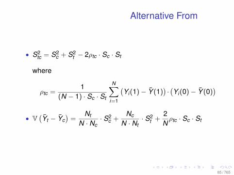
Alternative From
• S2tc = S2
c + S2t − 2ρtc · Sc · St
where
ρtc =1
(N − 1) · Sc · St
N∑i=1
(Yi(1)− Y (1)
)·(Yi(0)− Y (0)
)• V
(Yt − Yc
)=
Nt
N · Nc· S2
c +Nc
N · Nt· S2
t +2Nρtc · Sc · St
85 / 765
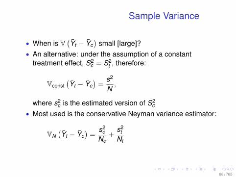
Sample Variance
• When is V(Yt − Yc
)small [large]?
• An alternative: under the assumption of a constanttreatment effect, S2
c = S2t , therefore:
Vconst(Yt − Yc
)=
s2
N,
where s2c is the estimated version of S2
c
• Most used is the conservative Neyman variance estimator:
VN(Yt − Yc
)=
s2c
Nc+
s2t
Nt
86 / 765
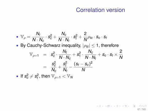
Correlation version
• Vρ =Nt
N · Nc· s2
c +Nc
N · Nt· s2
t +2Nρtc · sc · st
• By Cauchy-Schwarz inequality, |ρtc | ≤ 1, therefore
Vρ=1 = s2c ·
Nt
N · Nc+ s2
1 ·Nc
N · Nt+ sc · st ×
2N
=s2
cNc
+s2
tNt− (st − sc)2
N• If s2
c 6= s2t , then Vρ=1 < VN
87 / 765
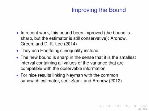
Improving the Bound
• In recent work, this bound been improved (the bound issharp, but the estimator is still conservative): Aronow,Green, and D. K. Lee (2014)
• They use Hoeffding’s inequality instead• The new bound is sharp in the sense that it is the smallest
interval containing all values of the variance that arecompatible with the observable information
• For nice results linking Neyman with the commonsandwich estimator, see: Samii and Aronow (2012)
88 / 765
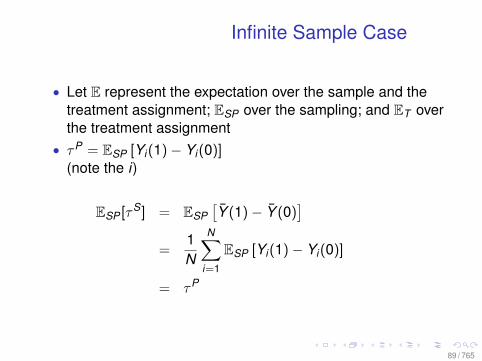
Infinite Sample Case
• Let E represent the expectation over the sample and thetreatment assignment; ESP over the sampling; and ET overthe treatment assignment
• τP = ESP [Yi(1)− Yi(0)](note the i)
ESP [τS] = ESP[Y (1)− Y (0)
]=
1N
N∑i=1
ESP [Yi(1)− Yi(0)]
= τP
89 / 765
Infinite Sample Case
• Let σ2 = ESP [S2]. Note:
σ2tc = VSP [Yi(1)− Yi(0)] = ESP
[(Yi(1)− Yi(0)− τP)2
]• Definition of the variance of the unit-level treatment in the
population implies:
VSP(τS) = VSP[Y (1)− Y (0)
]=σ2
tcN
(1)
• What is V(τ), where τ = Yt − Yc?
90 / 765
Infinite Sample Case
V(τ) = E[(
Yt − Yc − E[Yt − Yc
])2]
= E[(
Yt − Yc − ESP[Y (1)− Y (0)
])2],
With some algebra, and noting that
ET[Yt − Yc −
(Y (1)− Y (0)
)]= 0
We obtain
V(τ) = E[(
Yt − Yc − Y (1)− Y (0))2]
+ ESP
[(Y (1)− Y (0)− ESP [Y (1)− Y (0)]
)2]
91 / 765
Infinite Sample Case
V(τ) = E[(
Yt − Yc − Y (1)− Y (0))2]
+ ESP
[(Y (1)− Y (0)− ESP [Y (1)− Y (0)]
)2]
Recall that
ET
[(Yt − Yc − Y (1)− Y (0)
)2]
=S2
cNc
+S2
tNt− S2
tcN
And by simple results from sampling,
ESP
[S2
cNc
+S2
tNt− S2
tcN
]=σ2
cNc
+σ2
tNt− σ2
tcN
92 / 765
Infinite Sample Case
Also recall that
ESP
[(Y (1)− Y (0)− ESP [Y (1)− Y (0)]
)2]
=σ2
tcN
Therefore,
V(τ) = E[(
Yt − Yc − Y (1)− Y (0))2]
+ ESP
[(Y (1)− Y (0)− ESP [Y (1)− Y (0)]
)2]
=σ2
cNc
+σ2
tNt
93 / 765
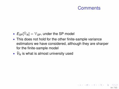
Comments
• ESP [VN ] = VSP , under the SP model• This does not hold for the other finite-sample variance
estimators we have considered, although they are sharperfor the finite-sample model
• VN is what is almost university used
94 / 765

95 / 765

96 / 765
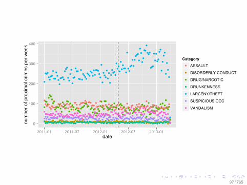
0
100
200
300
400
2011-01 2011-07 2012-01 2012-07 2013-01date
num
ber o
f pro
xim
al c
rimes
per
wee
k
CategoryASSAULT
DISORDERLY CONDUCT
DRUG/NARCOTIC
DRUNKENNESS
LARCENY/THEFT
SUSPICIOUS OCC
VANDALISM
97 / 765
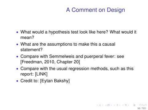
A Comment on Design
• What would a hypothesis test look like here? What would itmean?
• What are the assumptions to make this a causalstatement?
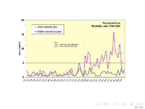
• Compare with Semmelweis and puerperal fever: see[Freedman, 2010, Chapter 20]
• Compare with the usual regression methods, such as thisreport: [LINK]
• Credit to: [Eytan Bakshy]
98 / 765
99 / 765

Kepler in a Stats Department
“I sometimes have a nightmare about Kepler. Suppose a few ofus were transported back in time to the year 1600, and wereinvited by the Emperor Rudolph II to set up an ImperialDepartment of Statistics in the court at Prague. Despairing ofthose circular orbits, Kepler enrolls in our department. We teachhim the general linear model, least squares, dummy variables,everything. He goes back to work, fits the best circular orbit forMars by least squares, puts in a dummy variable for theexceptional observation - and publishes. And that’s the end,right there in Prague at the beginning of the 17th century.”
Freedman, D.A. (1985). Statistics and the scientific method. In W.M. Mason & S.E. Fienberg (Eds.), Cohort analysisin social research: Beyond the identification problem (pp. 343-366). New York: Springer-Verlag.
100 / 765
Making Inference with AssumptionsFitting the Question
• The Fisher/Neyman approach required precise control overinterventions
• Neyman relied on what because the dominant way to doinference
• Fisher, and before him Pierce, Charles Sanders Peirce,outlined the way that is probably closest to the data
• With the growth of computing, a renaissance inpermutation inference
101 / 765
Lady Tasting Tea
• A canonical experiment which can be used to show thepower of randomization inference.
• The example is a special case of trying to figure out if twoproportions are different, which is a very common question.
• A lady (at Cambridge) claimed that by tasting a cup of teamade with milk she can determine whether the tea infusionor milk was added first (Fisher, 1935, pp. 11–25).
• The lady was B. Muriel Bristol-Roach, who was an algabiologist. [google scholar]
102 / 765
On Making Tea
• The precise way to make an optimal cup of tea has longbeen a contentious issue in China, India and Britain. e.g.,George Orwell had 11 rules for a perfect cup of tea.
• On the 100th anniversary of Orwell’s birth, the RoyalSociety of Chemistry decided to review Orwell’s rules.
103 / 765

100 Years Later: On Making Tea
• The Society sternly challenged Orwell’s advice that milk bepoured in after the tea. They noted that adding milk intohot water denatures the proteins—i.e., the proteins beginto unfold and clump together.
• The Society recommended that it is better to have thechilled milk at the bottom of the cup, so it can cool the teaas it is slowly poured in (BBC, 2003).
• In India, the milk is heated together with the water and thetea is infused into the milk and water mix.
• In the west, this is generally known as chai—the genericword for tea in Hindi which comes from the Chinesecharacter (pronounced chá in Mandarin) which is alsothe source word for tea in Punjabi, Russian, Swahili andmany other languages.
104 / 765
Fisher’s Experiment
The Lady:• is given eight cups of tea. Four of the cups have milk put in
first and four have tea put in first.• is presented the cups in random order without
replacement.• is told of this design so she, even if she has no ability to
discern the different types of cups, will select four cups tobe milk first and four to be tea first.
The Fisher exact test follows from examining the mechanics ofthe randomization which is done in this experiment.
105 / 765
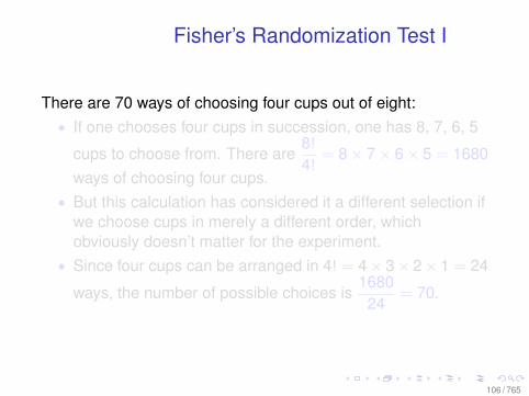
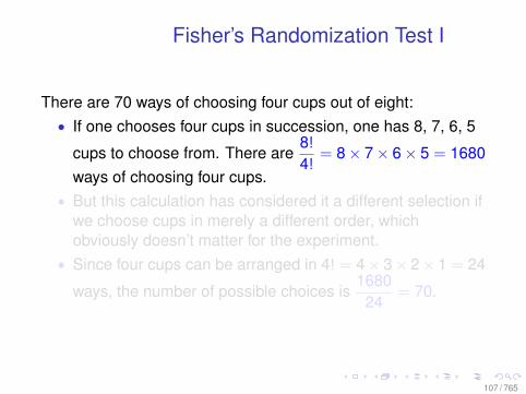
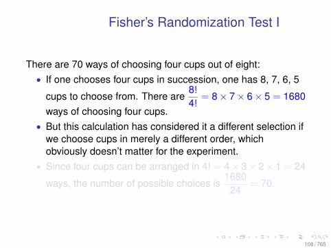
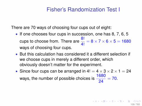
Fisher’s Randomization Test I
There are 70 ways of choosing four cups out of eight:• If one chooses four cups in succession, one has 8, 7, 6, 5
cups to choose from. There are8!
4!= 8× 7× 6× 5 = 1680
ways of choosing four cups.• But this calculation has considered it a different selection if
we choose cups in merely a different order, whichobviously doesn’t matter for the experiment.
• Since four cups can be arranged in 4! = 4× 3× 2× 1 = 24
ways, the number of possible choices is1680
24= 70.
106 / 765
Fisher’s Randomization Test I
There are 70 ways of choosing four cups out of eight:• If one chooses four cups in succession, one has 8, 7, 6, 5
cups to choose from. There are8!
4!= 8× 7× 6× 5 = 1680
ways of choosing four cups.• But this calculation has considered it a different selection if
we choose cups in merely a different order, whichobviously doesn’t matter for the experiment.
• Since four cups can be arranged in 4! = 4× 3× 2× 1 = 24
ways, the number of possible choices is1680
24= 70.
107 / 765
Fisher’s Randomization Test I
There are 70 ways of choosing four cups out of eight:• If one chooses four cups in succession, one has 8, 7, 6, 5
cups to choose from. There are8!
4!= 8× 7× 6× 5 = 1680
ways of choosing four cups.• But this calculation has considered it a different selection if
we choose cups in merely a different order, whichobviously doesn’t matter for the experiment.
• Since four cups can be arranged in 4! = 4× 3× 2× 1 = 24
ways, the number of possible choices is1680
24= 70.
108 / 765
Fisher’s Randomization Test I
There are 70 ways of choosing four cups out of eight:• If one chooses four cups in succession, one has 8, 7, 6, 5
cups to choose from. There are8!
4!= 8× 7× 6× 5 = 1680
ways of choosing four cups.• But this calculation has considered it a different selection if
we choose cups in merely a different order, whichobviously doesn’t matter for the experiment.
• Since four cups can be arranged in 4! = 4× 3× 2× 1 = 24
ways, the number of possible choices is1680
24= 70.
109 / 765
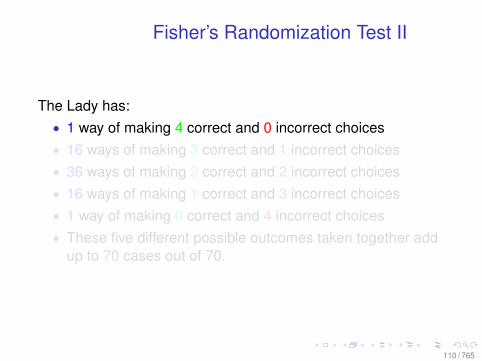
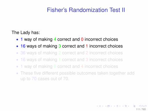
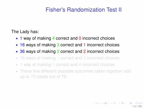
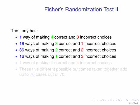
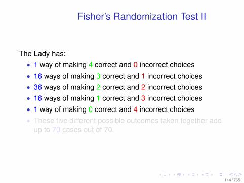
Fisher’s Randomization Test II
The Lady has:• 1 way of making 4 correct and 0 incorrect choices• 16 ways of making 3 correct and 1 incorrect choices• 36 ways of making 2 correct and 2 incorrect choices• 16 ways of making 1 correct and 3 incorrect choices• 1 way of making 0 correct and 4 incorrect choices• These five different possible outcomes taken together add
up to 70 cases out of 70.
110 / 765
Fisher’s Randomization Test II
The Lady has:• 1 way of making 4 correct and 0 incorrect choices• 16 ways of making 3 correct and 1 incorrect choices• 36 ways of making 2 correct and 2 incorrect choices• 16 ways of making 1 correct and 3 incorrect choices• 1 way of making 0 correct and 4 incorrect choices• These five different possible outcomes taken together add
up to 70 cases out of 70.
111 / 765
Fisher’s Randomization Test II
The Lady has:• 1 way of making 4 correct and 0 incorrect choices• 16 ways of making 3 correct and 1 incorrect choices• 36 ways of making 2 correct and 2 incorrect choices• 16 ways of making 1 correct and 3 incorrect choices• 1 way of making 0 correct and 4 incorrect choices• These five different possible outcomes taken together add
up to 70 cases out of 70.
112 / 765
Fisher’s Randomization Test II
The Lady has:• 1 way of making 4 correct and 0 incorrect choices• 16 ways of making 3 correct and 1 incorrect choices• 36 ways of making 2 correct and 2 incorrect choices• 16 ways of making 1 correct and 3 incorrect choices• 1 way of making 0 correct and 4 incorrect choices• These five different possible outcomes taken together add
up to 70 cases out of 70.
113 / 765
Fisher’s Randomization Test II
The Lady has:• 1 way of making 4 correct and 0 incorrect choices• 16 ways of making 3 correct and 1 incorrect choices• 36 ways of making 2 correct and 2 incorrect choices• 16 ways of making 1 correct and 3 incorrect choices• 1 way of making 0 correct and 4 incorrect choices• These five different possible outcomes taken together add
up to 70 cases out of 70.
114 / 765
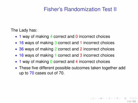
Fisher’s Randomization Test II
The Lady has:• 1 way of making 4 correct and 0 incorrect choices• 16 ways of making 3 correct and 1 incorrect choices• 36 ways of making 2 correct and 2 incorrect choices• 16 ways of making 1 correct and 3 incorrect choices• 1 way of making 0 correct and 4 incorrect choices• These five different possible outcomes taken together add
up to 70 cases out of 70.
115 / 765
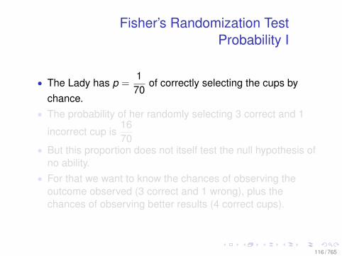
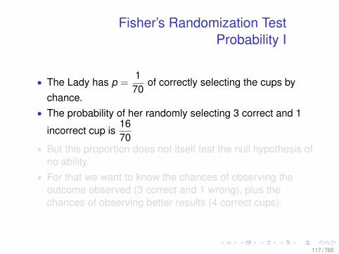
Fisher’s Randomization TestProbability I
• The Lady has p =1
70of correctly selecting the cups by
chance.• The probability of her randomly selecting 3 correct and 1
incorrect cup is1670
• But this proportion does not itself test the null hypothesis ofno ability.
• For that we want to know the chances of observing theoutcome observed (3 correct and 1 wrong), plus thechances of observing better results (4 correct cups).
116 / 765
Fisher’s Randomization TestProbability I
• The Lady has p =1
70of correctly selecting the cups by
chance.• The probability of her randomly selecting 3 correct and 1
incorrect cup is1670
• But this proportion does not itself test the null hypothesis ofno ability.
• For that we want to know the chances of observing theoutcome observed (3 correct and 1 wrong), plus thechances of observing better results (4 correct cups).
117 / 765
Fisher’s Randomization TestProbability I
• The Lady has p =1
70of correctly selecting the cups by
chance.• The probability of her randomly selecting 3 correct and 1
incorrect cup is1670
• But this proportion does not itself test the null hypothesis ofno ability.
• For that we want to know the chances of observing theoutcome observed (3 correct and 1 wrong), plus thechances of observing better results (4 correct cups).
118 / 765
Fisher’s Randomization TestProbability I
• The Lady has p =1
70of correctly selecting the cups by
chance.• The probability of her randomly selecting 3 correct and 1
incorrect cup is1670
• But this proportion does not itself test the null hypothesis ofno ability.
• For that we want to know the chances of observing theoutcome observed (3 correct and 1 wrong), plus thechances of observing better results (4 correct cups).
119 / 765
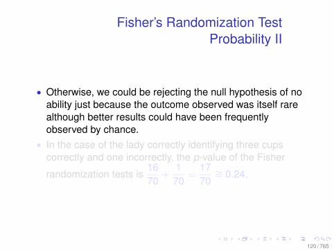
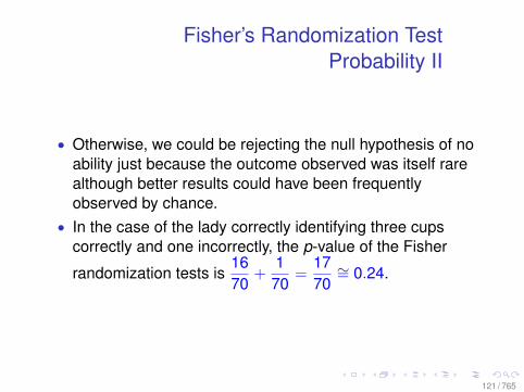
Fisher’s Randomization TestProbability II
• Otherwise, we could be rejecting the null hypothesis of noability just because the outcome observed was itself rarealthough better results could have been frequentlyobserved by chance.
• In the case of the lady correctly identifying three cupscorrectly and one incorrectly, the p-value of the Fisher
randomization tests is1670
+1
70=
1770∼= 0.24.
120 / 765
Fisher’s Randomization TestProbability II
• Otherwise, we could be rejecting the null hypothesis of noability just because the outcome observed was itself rarealthough better results could have been frequentlyobserved by chance.
• In the case of the lady correctly identifying three cupscorrectly and one incorrectly, the p-value of the Fisher
randomization tests is1670
+1
70=
1770∼= 0.24.
121 / 765
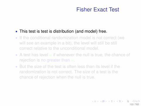
Fisher Exact Test
• This test is test is distribution (and model) free.• If the conditional randomization model is not correct (we
will see an example in a bit), the level will still be stillcorrect relative to the unconditional model.
• A test has level α if whenever the null is true, the chance ofrejection is no greater than α.
• But the size of the test is often less than its level if therandomization is not correct. The size of a test is thechance of rejection when the null is true.
122 / 765
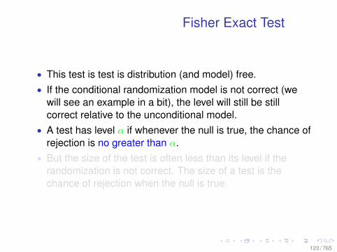
Fisher Exact Test
• This test is test is distribution (and model) free.• If the conditional randomization model is not correct (we
will see an example in a bit), the level will still be stillcorrect relative to the unconditional model.
• A test has level α if whenever the null is true, the chance ofrejection is no greater than α.
• But the size of the test is often less than its level if therandomization is not correct. The size of a test is thechance of rejection when the null is true.
123 / 765
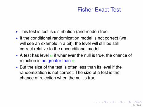
Fisher Exact Test
• This test is test is distribution (and model) free.• If the conditional randomization model is not correct (we
will see an example in a bit), the level will still be stillcorrect relative to the unconditional model.
• A test has level α if whenever the null is true, the chance ofrejection is no greater than α.
• But the size of the test is often less than its level if therandomization is not correct. The size of a test is thechance of rejection when the null is true.
124 / 765
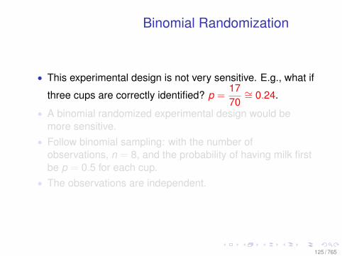
Binomial Randomization
• This experimental design is not very sensitive. E.g., what if
three cups are correctly identified? p =1770∼= 0.24.
• A binomial randomized experimental design would bemore sensitive.
• Follow binomial sampling: with the number ofobservations, n = 8, and the probability of having milk firstbe p = 0.5 for each cup.
• The observations are independent.
125 / 765
Binomial Randomization
• This experimental design is not very sensitive. E.g., what if
three cups are correctly identified? p =1770∼= 0.24.
• A binomial randomized experimental design would bemore sensitive.
• Follow binomial sampling: with the number ofobservations, n = 8, and the probability of having milk firstbe p = 0.5 for each cup.
• The observations are independent.
126 / 765
Binomial Randomization
• This experimental design is not very sensitive. E.g., what if
three cups are correctly identified? p =1770∼= 0.24.
• A binomial randomized experimental design would bemore sensitive.
• Follow binomial sampling: with the number ofobservations, n = 8, and the probability of having milk firstbe p = 0.5 for each cup.
• The observations are independent.
127 / 765
Binomial Randomization
• This experimental design is not very sensitive. E.g., what if
three cups are correctly identified? p =1770∼= 0.24.
• A binomial randomized experimental design would bemore sensitive.
• Follow binomial sampling: with the number ofobservations, n = 8, and the probability of having milk firstbe p = 0.5 for each cup.
• The observations are independent.
128 / 765
Binomial Randomization II
• The chance of classifying correctly eight cups binomialrandomized is 1 in 28 = 256, which is significantly lowerthan 1 in 70.
• There are 8 ways in 256 (p=0.032) of incorrectly classifyingonly one cup.
• Unlike in the canonical experiment, case of having bothmargins fixed, in the case of the binomial design, theexperiment is sensitive enough to reject the null hypothesisif the lady makes a single mistake
129 / 765
Binomial Randomization II
• The chance of classifying correctly eight cups binomialrandomized is 1 in 28 = 256, which is significantly lowerthan 1 in 70.
• There are 8 ways in 256 (p=0.032) of incorrectly classifyingonly one cup.
• Unlike in the canonical experiment, case of having bothmargins fixed, in the case of the binomial design, theexperiment is sensitive enough to reject the null hypothesisif the lady makes a single mistake
130 / 765
Binomial Randomization II
• The chance of classifying correctly eight cups binomialrandomized is 1 in 28 = 256, which is significantly lowerthan 1 in 70.
• There are 8 ways in 256 (p=0.032) of incorrectly classifyingonly one cup.
• Unlike in the canonical experiment, case of having bothmargins fixed, in the case of the binomial design, theexperiment is sensitive enough to reject the null hypothesisif the lady makes a single mistake
131 / 765

Comments
• The extra sensitively comes purely from the design, andnot from more data.
• The binomial design is more sensitive, but there may besome reasons to prefer the design with fixed margins. E.g.,there is a chance with the binomial design that all cupswould be treated alike.
132 / 765
Comments
• The extra sensitively comes purely from the design, andnot from more data.
• The binomial design is more sensitive, but there may besome reasons to prefer the design with fixed margins. E.g.,there is a chance with the binomial design that all cupswould be treated alike.
133 / 765

Sharp Null
• Fisherian inference proceeds using a sharp null—i.e., all ofthe potential outcomes under the null are specified.
• Is the above true for the usuall null hypothesis that τ = 0?Under the sharp null the equivilant is: τi = 0 ∀ i .
• But note that we can pick any sharp null we wish—e.g.,τi = −1 ∀ i < 10 and τi = 20 ∀ i > 10.
134 / 765
Sharp Null
• Fisherian inference proceeds using a sharp null—i.e., all ofthe potential outcomes under the null are specified.
• Is the above true for the usuall null hypothesis that τ = 0?Under the sharp null the equivilant is: τi = 0 ∀ i .
• But note that we can pick any sharp null we wish—e.g.,τi = −1 ∀ i < 10 and τi = 20 ∀ i > 10.
135 / 765
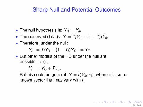
Sharp Null and Potential Outcomes
• The null hypothesis is: Yi1 = Yi0
• The observed data is: Yi = TiYi1 + (1− Ti)Yi0
• Therefore, under the null:Yi = TiYi1 + (1− Ti)Yi0 = Yi0
• But other models of the PO under the null arepossible—e.g.,
Yi = Yi0 + Tiτ0,
But his could be general: Y = f (Yi0, τi), where τ is someknown vector that may vary with i .
136 / 765
General Procedure
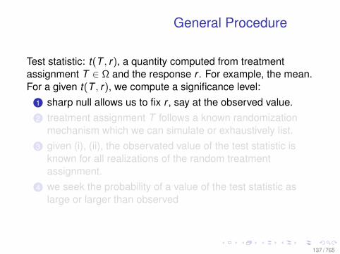
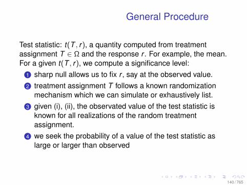
Test statistic: t(T , r), a quantity computed from treatmentassignment T ∈ Ω and the response r . For example, the mean.For a given t(T , r), we compute a significance level:
1 sharp null allows us to fix r , say at the observed value.2 treatment assignment T follows a known randomization
mechanism which we can simulate or exhaustively list.3 given (i), (ii), the observated value of the test statistic is
known for all realizations of the random treatmentassignment.
4 we seek the probability of a value of the test statistic aslarge or larger than observed
137 / 765
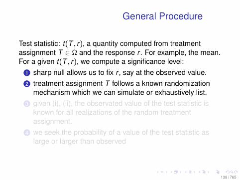
General Procedure
Test statistic: t(T , r), a quantity computed from treatmentassignment T ∈ Ω and the response r . For example, the mean.For a given t(T , r), we compute a significance level:
1 sharp null allows us to fix r , say at the observed value.2 treatment assignment T follows a known randomization
mechanism which we can simulate or exhaustively list.3 given (i), (ii), the observated value of the test statistic is
known for all realizations of the random treatmentassignment.
4 we seek the probability of a value of the test statistic aslarge or larger than observed
138 / 765
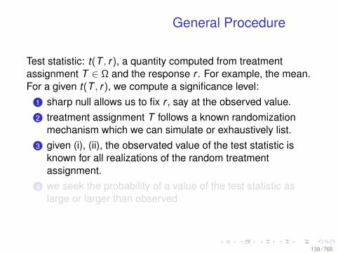
General Procedure
Test statistic: t(T , r), a quantity computed from treatmentassignment T ∈ Ω and the response r . For example, the mean.For a given t(T , r), we compute a significance level:
1 sharp null allows us to fix r , say at the observed value.2 treatment assignment T follows a known randomization
mechanism which we can simulate or exhaustively list.3 given (i), (ii), the observated value of the test statistic is
known for all realizations of the random treatmentassignment.
4 we seek the probability of a value of the test statistic aslarge or larger than observed
139 / 765
General Procedure
Test statistic: t(T , r), a quantity computed from treatmentassignment T ∈ Ω and the response r . For example, the mean.For a given t(T , r), we compute a significance level:
1 sharp null allows us to fix r , say at the observed value.2 treatment assignment T follows a known randomization
mechanism which we can simulate or exhaustively list.3 given (i), (ii), the observated value of the test statistic is
known for all realizations of the random treatmentassignment.
4 we seek the probability of a value of the test statistic aslarge or larger than observed
140 / 765
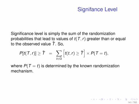
Signifance Level
Significance level is simply the sum of the randomizationprobabilities that lead to values of t(T , r) greater than or equalto the observed value T . So,
P[t(T , r)] ≥ T =∑t∈Ω
[t(t , r) ≥ T
]× P(T = t),
where P(T = t) is determined by the known randomizationmechanism.
141 / 765
Further Reading
See Rosenbaum (2002). Observational Studies, chp2 and
Rosenbaum, P. R. (2002). “Covariance adjustment inrandomized experiments and observational studies.” StatisticalScience 17 286–327 (with discussion).
Simple introduction: Michael D. Ernst (2004). “PermutationMethods: A Basis for Exact Inference.” Statistical Science 19:4676–685.
142 / 765
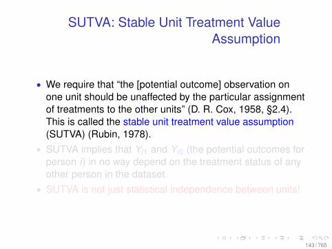
SUTVA: Stable Unit Treatment ValueAssumption
• We require that “the [potential outcome] observation onone unit should be unaffected by the particular assignmentof treatments to the other units” (D. R. Cox, 1958, §2.4).This is called the stable unit treatment value assumption(SUTVA) (Rubin, 1978).
• SUTVA implies that Yi1 and Yi0 (the potential outcomes forperson i) in no way depend on the treatment status of anyother person in the dataset.
• SUTVA is not just statistical independence between units!
143 / 765
SUTVA: Stable Unit Treatment ValueAssumption
• We require that “the [potential outcome] observation onone unit should be unaffected by the particular assignmentof treatments to the other units” (D. R. Cox, 1958, §2.4).This is called the stable unit treatment value assumption(SUTVA) (Rubin, 1978).
• SUTVA implies that Yi1 and Yi0 (the potential outcomes forperson i) in no way depend on the treatment status of anyother person in the dataset.
• SUTVA is not just statistical independence between units!
144 / 765
SUTVA: Stable Unit Treatment ValueAssumption
• We require that “the [potential outcome] observation onone unit should be unaffected by the particular assignmentof treatments to the other units” (D. R. Cox, 1958, §2.4).This is called the stable unit treatment value assumption(SUTVA) (Rubin, 1978).
• SUTVA implies that Yi1 and Yi0 (the potential outcomes forperson i) in no way depend on the treatment status of anyother person in the dataset.
• SUTVA is not just statistical independence between units!
145 / 765
SUTVA: Stable Unit Treatment ValueAssumption
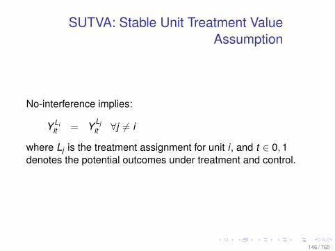
No-interference implies:
Y Liit = Y Lj
it ∀j 6= i
where Lj is the treatment assignment for unit i , and t ∈ 0,1denotes the potential outcomes under treatment and control.
146 / 765
SUTVA: Stable Unit Treatment ValueAssumption
• Causal inference relies on a counterfactual of interest(Sekhon, 2004), and the one which is most obviouslyrelevant for political information is “how would Jane havevoted if she were better informed?”.
• There are other theoretically interesting counterfactualswhich, because of SUTVA, I do not know how toempirically answer such as “who would have won the lastelection if everyone were well informed?”.
147 / 765
SUTVA: Stable Unit Treatment ValueAssumption
• Causal inference relies on a counterfactual of interest(Sekhon, 2004), and the one which is most obviouslyrelevant for political information is “how would Jane havevoted if she were better informed?”.
• There are other theoretically interesting counterfactualswhich, because of SUTVA, I do not know how toempirically answer such as “who would have won the lastelection if everyone were well informed?”.
148 / 765
Another Example: Florida 2004 VotingTechnology
• In the aftermath of the 2004 Presidential election, manyresearchers argued that the optical voting machines thatare used in a majority of Florida counties caused JohnKerry to receive fewer votes than “Direct RecordingElectronic” (DRE) voting machines (Hout et al.).
• Hout et al. used a regression model to arrive at thisconclusion.
• Problem: The distributions of counties were are profoundlyimbalanced
149 / 765
Another Example: Florida 2004 VotingTechnology
• In the aftermath of the 2004 Presidential election, manyresearchers argued that the optical voting machines thatare used in a majority of Florida counties caused JohnKerry to receive fewer votes than “Direct RecordingElectronic” (DRE) voting machines (Hout et al.).
• Hout et al. used a regression model to arrive at thisconclusion.
• Problem: The distributions of counties were are profoundlyimbalanced
150 / 765
Another Example: Florida 2004 VotingTechnology
• In the aftermath of the 2004 Presidential election, manyresearchers argued that the optical voting machines thatare used in a majority of Florida counties caused JohnKerry to receive fewer votes than “Direct RecordingElectronic” (DRE) voting machines (Hout et al.).
• Hout et al. used a regression model to arrive at thisconclusion.
• Problem: The distributions of counties were are profoundlyimbalanced
151 / 765
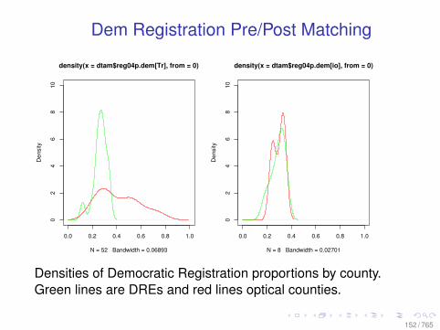
Dem Registration Pre/Post Matching
0.0 0.2 0.4 0.6 0.8 1.0
02
46
810
density(x = dtam$reg04p.dem[Tr], from = 0)
N = 52 Bandwidth = 0.06893
Den
sity
0.0 0.2 0.4 0.6 0.8 1.00
24
68
10
density(x = dtam$reg04p.dem[io], from = 0)
N = 8 Bandwidth = 0.02701
Den
sity
Densities of Democratic Registration proportions by county.Green lines are DREs and red lines optical counties.
152 / 765
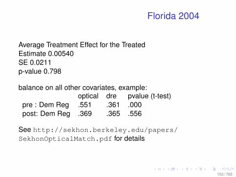
Florida 2004
Average Treatment Effect for the TreatedEstimate 0.00540SE 0.0211p-value 0.798
balance on all other covariates, example:optical dre pvalue (t-test)
pre : Dem Reg .551 .361 .000post: Dem Reg .369 .365 .556
See http://sekhon.berkeley.edu/papers/SekhonOpticalMatch.pdf for details
153 / 765
Matching
• The nonparametric way to condition on X is to exactlymatch on the covariates.
• This approach fails in finite samples if the dimensionality ofX is large.
• If X consists of more than one continuous variable, exactmatching is inefficient: matching estimators with a fixednumber of matches do not reach the semi-parametricefficiency bound for average treatment effects (Abadie andG. Imbens, 2006).
• An alternative way to condition on X is to match on theprobability of being assigned to treatment—i.e., thepropensity score (P. R. Rosenbaum and Rubin, 1983). Thepropensity score is just one dimensional.
154 / 765
Matching
• The nonparametric way to condition on X is to exactlymatch on the covariates.
• This approach fails in finite samples if the dimensionality ofX is large.
• If X consists of more than one continuous variable, exactmatching is inefficient: matching estimators with a fixednumber of matches do not reach the semi-parametricefficiency bound for average treatment effects (Abadie andG. Imbens, 2006).
• An alternative way to condition on X is to match on theprobability of being assigned to treatment—i.e., thepropensity score (P. R. Rosenbaum and Rubin, 1983). Thepropensity score is just one dimensional.
155 / 765
Matching
• The nonparametric way to condition on X is to exactlymatch on the covariates.
• This approach fails in finite samples if the dimensionality ofX is large.
• If X consists of more than one continuous variable, exactmatching is inefficient: matching estimators with a fixednumber of matches do not reach the semi-parametricefficiency bound for average treatment effects (Abadie andG. Imbens, 2006).
• An alternative way to condition on X is to match on theprobability of being assigned to treatment—i.e., thepropensity score (P. R. Rosenbaum and Rubin, 1983). Thepropensity score is just one dimensional.
156 / 765
Matching
• The nonparametric way to condition on X is to exactlymatch on the covariates.
• This approach fails in finite samples if the dimensionality ofX is large.
• If X consists of more than one continuous variable, exactmatching is inefficient: matching estimators with a fixednumber of matches do not reach the semi-parametricefficiency bound for average treatment effects (Abadie andG. Imbens, 2006).
• An alternative way to condition on X is to match on theprobability of being assigned to treatment—i.e., thepropensity score (P. R. Rosenbaum and Rubin, 1983). Thepropensity score is just one dimensional.
157 / 765
Propensity Score (pscore)
• More formally the propensity score is:Pr(T = 1|X ) = E(T |X )
• It is a one-dimensional balancing score• It helps to reduces the difficulty of matching• If one balances the propensity score, one balances on the
confounders X• But if the pscore is not known, it must be estimated.• How do we know if we estimate the correct propensity
score?• It is a tautology—but we can observe some implications
158 / 765
Neyman/Fisher versus OLS
• Compare the classical OLS assumptions with those from acanonical experiment described by Fisher (1935): “TheLady Tasting Tea.”
• Compare the classical OLS assumptions with those fromthe Neyman model
159 / 765
Classical OLS Assumptions
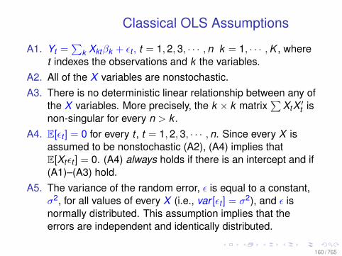
A1. Yt =∑
k Xktβk + εt , t = 1,2,3, · · · ,n k = 1, · · · ,K , wheret indexes the observations and k the variables.
A2. All of the X variables are nonstochastic.A3. There is no deterministic linear relationship between any of
the X variables. More precisely, the k × k matrix∑
XtX ′t isnon-singular for every n > k .
A4. E[εt ] = 0 for every t , t = 1,2,3, · · · ,n. Since every X isassumed to be nonstochastic (A2), (A4) implies thatE[Xtεt ] = 0. (A4) always holds if there is an intercept and if(A1)–(A3) hold.
A5. The variance of the random error, ε is equal to a constant,σ2, for all values of every X (i.e., var [εt ] = σ2), and ε isnormally distributed. This assumption implies that theerrors are independent and identically distributed.
160 / 765
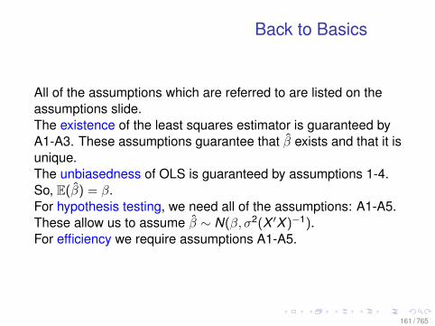
Back to Basics
All of the assumptions which are referred to are listed on theassumptions slide.The existence of the least squares estimator is guaranteed byA1-A3. These assumptions guarantee that β exists and that it isunique.The unbiasedness of OLS is guaranteed by assumptions 1-4.So, E(β) = β.For hypothesis testing, we need all of the assumptions: A1-A5.These allow us to assume β ∼ N(β, σ2(X ′X )−1).For efficiency we require assumptions A1-A5.
161 / 765
Correct Specification Assumption
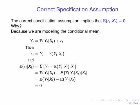
The correct specification assumption implies that E(εt |Xt ) = 0.Why?Because we are modeling the conditional mean.
Yt = E(Yt |Xt ) + εt
Then
εt = Yt − E(Yt |Xt )
and
E(εt |Xt ) = E [Yt − E(Yt |Xt )|Xt ]
= E(Yt |Xt )− E [E(Yt |Xt )|Xt ]
= E(Yt |Xt )− E(Yt |Xt )
= 0
162 / 765
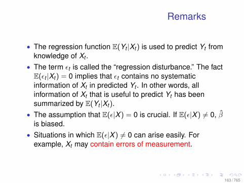
Remarks
• The regression function E(Yt |Xt ) is used to predict Yt fromknowledge of Xt .
• The term εt is called the “regression disturbance.” The factE(εt |Xt ) = 0 implies that εt contains no systematicinformation of Xt in predicted Yt . In other words, allinformation of Xt that is useful to predict Yt has beensummarized by E(Yt |Xt ).
• The assumption that E(ε|X ) = 0 is crucial. If E(ε|X ) 6= 0, βis biased.
• Situations in which E(ε|X ) 6= 0 can arise easily. Forexample, Xt may contain errors of measurement.
163 / 765
Recall Post-Treatment Bias
The lesson of the lagged differences example is to not ask toomuch from regression. See:http://sekhon.berkeley.edu/causalinf/R/difference1.R.
Many lessons follow from this. One of the most important is theissue of post-treatment bias. Post-treatment variables are thosewhich are a consequence of the treatment of interest. Hence,they will be correlated with the treatment unless their values arethe same under treatment and control.
164 / 765
Recall Post-Treatment Bias
The lesson of the lagged differences example is to not ask toomuch from regression. See:http://sekhon.berkeley.edu/causalinf/R/difference1.R.
Many lessons follow from this. One of the most important is theissue of post-treatment bias. Post-treatment variables are thosewhich are a consequence of the treatment of interest. Hence,they will be correlated with the treatment unless their values arethe same under treatment and control.
165 / 765
Some Intuition: Let’s derive OLS withtwo covars
• See my Government 1000 lecture notes from Harvard orany intro text book for more details
• Let’s restrict ourselves to two covariates to help with theintuition
• Our goal is to minimize∑n
i (Yi − Yi)2, where
Yi = α + β1X1i + β2X2i .• We can do this by calculating the partial derivaties with
respect to the three unknown parameters α, β1, β2,equating each to 0 and solving.
• To simplify: deviate the observed variables by their means.These mean deviated variables are denoted by yi , x1i andx2i .
166 / 765
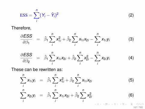
ESS =n∑i
(Yi − Yi)2 (2)
Therefore,
∂ESS∂β1
= β1
n∑i
x21i + β2
n∑i
x1ix2i −n∑i
x1iyi (3)
∂ESS∂β2
= β1
n∑i
x1ix2i + β2
n∑i
x22i −
n∑i
x2iyi (4)
These can be rewritten as:n∑i
x1iyi = β1
n∑i
x21i + β2
n∑i
x1ix2i (5)
n∑i
x2iyi = β1
n∑i
x1ix2i + β2
n∑i
x22i (6)
167 / 765
Recall:n∑i
x1iyi = β1
n∑i
x21i + β2
n∑i
x1ix2i (7)
n∑i
x2iyi = β1
n∑i
x1ix2i + β2
n∑i
x22i (8)
To solve, we multiply Equation 7 by∑n
i x22i and Equation 8 by∑n
i x1ix2i and subtract the latter from the former.
168 / 765
Thus,
β1 =(∑n
i x1iyi)(∑n
i x2x2i)− (
∑ni x2iyi)(
∑ni x1ix2i)
(∑n
i x21i)(∑n
i x22i)− (
∑ni x1ix2i)2
(9)
And
β2 =(∑n
i x2iyi)(∑n
i x2x1i)− (
∑ni x1iyi)(
∑ni x1ix2i)
(∑n
i x21i)(∑n
i x22i)− (
∑ni x1ix2i)2
(10)
If we do the same for α we find that:
α = Y − β1X1 − β2X2 (11)
169 / 765
The equations for the estimates of β1 and β2 can be rewrittenas:
β1 =cov(X1i ,Yi) var(X2i) − cov(X2i ,Yi) cov(X1i ,X2i)
var(X1i) var(X2i) − [cov(X1i ,X2i)]2
And,
β2 =cov(X2i ,Yi) var(X1i) − cov(X1i ,Yi) cov(X1i ,X2i)
var(X1i) var(X2i) − [cov(X1i ,X2i)]2
To understand the post-treatment problem in the motivatingexample see:http://sekhon.berkeley.edu/causalinf/R/part1.R
170 / 765
Post-Treatment Bias Revisited
• The discussion about post-treatment bias is related to whycertain causal questions are difficult if not impossible toanswer (Holland, 1986).
• For example, what is the causal effect of a education onvoting? How do we answer this using a cross-sectionalsurvey?
• A more charged examples: race and sex. What ispost-treatment in gender discrimination cases?
171 / 765
Post-Treatment Bias Revisited
• The discussion about post-treatment bias is related to whycertain causal questions are difficult if not impossible toanswer (Holland, 1986).
• For example, what is the causal effect of a education onvoting? How do we answer this using a cross-sectionalsurvey?
• A more charged examples: race and sex. What ispost-treatment in gender discrimination cases?
172 / 765
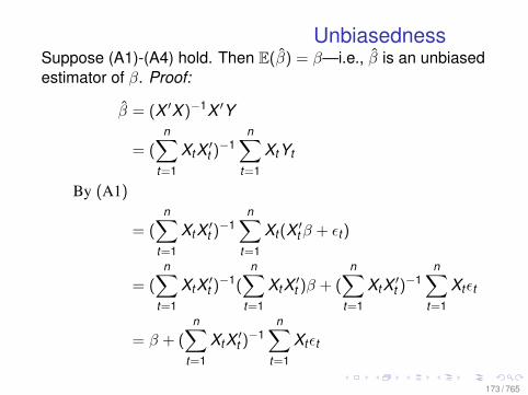
UnbiasednessSuppose (A1)-(A4) hold. Then E(β) = β—i.e., β is an unbiasedestimator of β. Proof:
β = (X ′X )−1X ′Y
= (n∑
t=1
XtX ′t )−1n∑
t=1
XtYt
By (A1)
= (n∑
t=1
XtX ′t )−1n∑
t=1
Xt (X ′t β + εt )
= (n∑
t=1
XtX ′t )−1(n∑
t=1
XtX ′t )β + (n∑
t=1
XtX ′t )−1n∑
t=1
Xtεt
= β + (n∑
t=1
XtX ′t )−1n∑
t=1
Xtεt
173 / 765
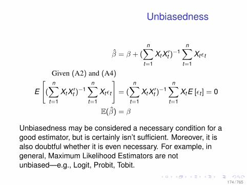
Unbiasedness
β = β + (n∑
t=1
XtX ′t )−1n∑
t=1
Xtεt
Given (A2) and (A4)
E
[(
n∑t=1
XtX ′t )−1n∑
t=1
Xtεt
]= (
n∑t=1
XtX ′t )−1n∑
t=1
XtE [εt ] = 0
E(β) = β
Unbiasedness may be considered a necessary condition for agood estimator, but is certainly isn’t sufficient. Moreover, it isalso doubtful whether it is even necessary. For example, ingeneral, Maximum Likelihood Estimators are notunbiased—e.g., Logit, Probit, Tobit.
174 / 765
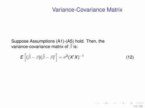
Variance-Covariance Matrix
Suppose Assumptions (A1)-(A5) hold. Then, thevariance-covariance matrix of β is:
E[(β − β)(β − β)′
]= σ2(X ′X )−1 (12)
175 / 765
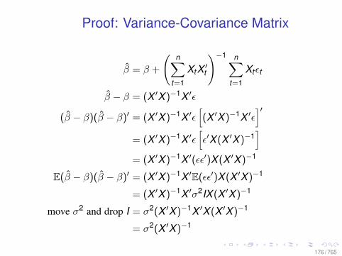
Proof: Variance-Covariance Matrix
β = β +
(n∑
t=1
XtX ′t
)−1 n∑t=1
Xtεt
β − β = (X ′X )−1X ′ε
(β − β)(β − β)′ = (X ′X )−1X ′ε[(X ′X )−1X ′ε
]′= (X ′X )−1X ′ε
[ε′X (X ′X )−1
]= (X ′X )−1X ′(εε′)X (X ′X )−1
E(β − β)(β − β)′ = (X ′X )−1X ′E(εε′)X (X ′X )−1
= (X ′X )−1X ′σ2IX (X ′X )−1
move σ2 and drop I = σ2(X ′X )−1X ′X (X ′X )−1
= σ2(X ′X )−1
176 / 765
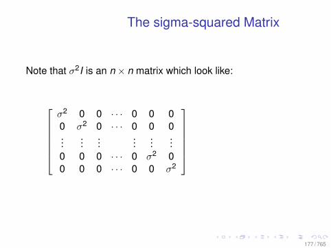
The sigma-squared Matrix
Note that σ2I is an n × n matrix which look like:
σ2 0 0 · · · 0 0 00 σ2 0 · · · 0 0 0...
......
......
...0 0 0 · · · 0 σ2 00 0 0 · · · 0 0 σ2
177 / 765
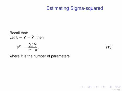
Estimating Sigma-squared
Recall that:Let εi = Yi − Yi , then
σ2 =
∑ε2i
n − k, (13)
where k is the number of parameters.
178 / 765
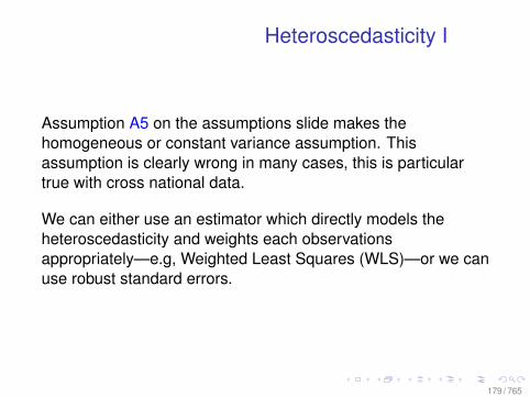
Heteroscedasticity I
Assumption A5 on the assumptions slide makes thehomogeneous or constant variance assumption. Thisassumption is clearly wrong in many cases, this is particulartrue with cross national data.
We can either use an estimator which directly models theheteroscedasticity and weights each observationsappropriately—e.g, Weighted Least Squares (WLS)—or we canuse robust standard errors.
179 / 765
Heteroscedasticity II
The OLS estimator is unbiased (and consistent) when there isheteroscedasticity, but it is not efficient. We say that α is anefficient unbiased estimator if for a given sample size thevariance of α is smaller than (or equal to) the variance of anyother unbiased estimator.
Why is OLS still unbiased? Recall that when we proved thatOLS is unbiased, the variance terms played no part in theproof—i.e., Assumption A5 played no part.
180 / 765
Univariate Matching
• Assume that we obtain conditional independence if wecondition on one confounder, XiG, where i indexes theobservation and G ∈ T ,C denotes the treatment orcontrol group.
• Say we wish to compare two matched pairs to estimateATT, τi ′ = Yi1 − Yi ′0, where ’ denotes the matchedobservation.
• Matched pairs can be used to estimate τ because thetreatment observation reveals Yi1 and the controlobservation Yi0 under conditional exchangeability.
• Bias in the estimate of τi ′ is assumed to be some unknownincreasing function of |XiT − Xi ′C |.
181 / 765
Univariate Matching
• Assume that we obtain conditional independence if wecondition on one confounder, XiG, where i indexes theobservation and G ∈ T ,C denotes the treatment orcontrol group.
• Say we wish to compare two matched pairs to estimateATT, τi ′ = Yi1 − Yi ′0, where ’ denotes the matchedobservation.
• Matched pairs can be used to estimate τ because thetreatment observation reveals Yi1 and the controlobservation Yi0 under conditional exchangeability.
• Bias in the estimate of τi ′ is assumed to be some unknownincreasing function of |XiT − Xi ′C |.
182 / 765
Univariate Matching
• Assume that we obtain conditional independence if wecondition on one confounder, XiG, where i indexes theobservation and G ∈ T ,C denotes the treatment orcontrol group.
• Say we wish to compare two matched pairs to estimateATT, τi ′ = Yi1 − Yi ′0, where ’ denotes the matchedobservation.
• Matched pairs can be used to estimate τ because thetreatment observation reveals Yi1 and the controlobservation Yi0 under conditional exchangeability.
• Bias in the estimate of τi ′ is assumed to be some unknownincreasing function of |XiT − Xi ′C |.
183 / 765
Univariate Matching
• Assume that we obtain conditional independence if wecondition on one confounder, XiG, where i indexes theobservation and G ∈ T ,C denotes the treatment orcontrol group.
• Say we wish to compare two matched pairs to estimateATT, τi ′ = Yi1 − Yi ′0, where ’ denotes the matchedobservation.
• Matched pairs can be used to estimate τ because thetreatment observation reveals Yi1 and the controlobservation Yi0 under conditional exchangeability.
• Bias in the estimate of τi ′ is assumed to be some unknownincreasing function of |XiT − Xi ′C |.
184 / 765
Univariate Matching
• We can then minimize our bias in τi ′ and hence ˆτ byminimizing |XiT − Xi ′C | for each matched pair.
• Can be minimized non-parametrically by “nearest neighbormatching” (NN). The case with replacement is simple.
• With NN matching we just match the nearest Xi ′C to agiven XiT .
• For ATT, we match every XiT with the nearest Xi ′C .• For ATC, we match every XiC with the nearest Xi ′T .• For ATE, we match every XiT with the nearest Xi ′C AND
match every XiC with the nearest Xi ′T .• Let’s walk through some examples: nn1.R
185 / 765
Univariate Matching
• We can then minimize our bias in τi ′ and hence ˆτ byminimizing |XiT − Xi ′C | for each matched pair.
• Can be minimized non-parametrically by “nearest neighbormatching” (NN). The case with replacement is simple.
• With NN matching we just match the nearest Xi ′C to agiven XiT .
• For ATT, we match every XiT with the nearest Xi ′C .• For ATC, we match every XiC with the nearest Xi ′T .• For ATE, we match every XiT with the nearest Xi ′C AND
match every XiC with the nearest Xi ′T .• Let’s walk through some examples: nn1.R
186 / 765
Univariate Matching
• We can then minimize our bias in τi ′ and hence ˆτ byminimizing |XiT − Xi ′C | for each matched pair.
• Can be minimized non-parametrically by “nearest neighbormatching” (NN). The case with replacement is simple.
• With NN matching we just match the nearest Xi ′C to agiven XiT .
• For ATT, we match every XiT with the nearest Xi ′C .• For ATC, we match every XiC with the nearest Xi ′T .• For ATE, we match every XiT with the nearest Xi ′C AND
match every XiC with the nearest Xi ′T .• Let’s walk through some examples: nn1.R
187 / 765
Univariate Matching
• We can then minimize our bias in τi ′ and hence ˆτ byminimizing |XiT − Xi ′C | for each matched pair.
• Can be minimized non-parametrically by “nearest neighbormatching” (NN). The case with replacement is simple.
• With NN matching we just match the nearest Xi ′C to agiven XiT .
• For ATT, we match every XiT with the nearest Xi ′C .• For ATC, we match every XiC with the nearest Xi ′T .• For ATE, we match every XiT with the nearest Xi ′C AND
match every XiC with the nearest Xi ′T .• Let’s walk through some examples: nn1.R
188 / 765
Univariate Matching
• We can then minimize our bias in τi ′ and hence ˆτ byminimizing |XiT − Xi ′C | for each matched pair.
• Can be minimized non-parametrically by “nearest neighbormatching” (NN). The case with replacement is simple.
• With NN matching we just match the nearest Xi ′C to agiven XiT .
• For ATT, we match every XiT with the nearest Xi ′C .• For ATC, we match every XiC with the nearest Xi ′T .• For ATE, we match every XiT with the nearest Xi ′C AND
match every XiC with the nearest Xi ′T .• Let’s walk through some examples: nn1.R
189 / 765
Univariate Matching
• We can then minimize our bias in τi ′ and hence ˆτ byminimizing |XiT − Xi ′C | for each matched pair.
• Can be minimized non-parametrically by “nearest neighbormatching” (NN). The case with replacement is simple.
• With NN matching we just match the nearest Xi ′C to agiven XiT .
• For ATT, we match every XiT with the nearest Xi ′C .• For ATC, we match every XiC with the nearest Xi ′T .• For ATE, we match every XiT with the nearest Xi ′C AND
match every XiC with the nearest Xi ′T .• Let’s walk through some examples: nn1.R
190 / 765
Generalized Linear Models
Generalized linear models (GLMs) extend linear models toaccommodate both non-normal distributions andtransformations to linearity. GLMs allow unified treatment ofstatistical methodology for several important classes of models.
191 / 765
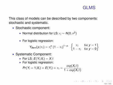
GLMS
This class of models can be described by two components:stochastic and systematic.• Stochastic component:
• Normal distribution for LS: εi ∼ N(0, σ2)
• For logistic regression:
YBern(yi |πi ) = πyii (1− πi )
1−yi
πi for y = 1
1− πi for y = 0
• Systematic Component:
• For LS: E(Yi |Xi ) = Xβ• For logistic regression:
Pr(Yi = 1|Xi ) ≡ E(Yi ) ≡ πi =exp(Xiβ)
1 + exp(Xiβ)
192 / 765
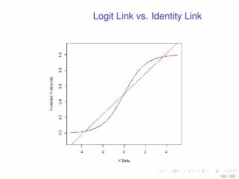
Logit Link vs. Identity Link
193 / 765
Logit Link vs. Identity Link
The black line is the logistic fitted values and the red line is fromOLS (the identity link). For R code see, logit1.R
OLS goes unbounded, which we know cannot happen!
194 / 765
Defining Assumptions
A generalized linear model may be described by the followingassumptions:
• There is a response Y observed independently at fixedvalues of stimulus variables X1, · · · ,Xk .
• The stimulus variables may only influence the distributionof Y through a single linear function called the linearpredictor η = β1X1 + · · ·+ βkXk .
195 / 765
Defining Assumptions
• The distribution of Y has density of the form
f (Yi ; θi , φ) = exp[AiYiθi − γ(θi)/φ+ τ(Yi , φ/Ai)], (14)
where φ is a scale parameter (possibly known). Ai is aknown prior weight and parameter θi depends upon thelinear predictor.
This is the exponential family of distributions. Most of thedistributions you know are part of this family including thenormal, binomial and Poisson.
196 / 765
Models of the Mean
The mean µ = E(Y ) is a smooth invertible function of the linearpredictor:
µ = m(η), (15)η = m−1(µ) = l(µ), (16)
where the inverse function l(·) is called the link function
197 / 765
Models of the Mean: examples
For LS we use the identity link (also called the canonical link):l(µ) = µ. Thus,
Xiβ = ηi = m(µi) = µi = E(Yi)
For logistic regression we use the logit link:
l(µ) = log(
π
1− π
). Thus,
Xiβ = ηi = m(µi) =exp(ηi)
1 + exp(ηi)= µi = E(Yi) = Pr(Yi = 1|Xi),
note thatexp(ηi)
1 + exp(ηi)is the inverse logit link.
198 / 765
GLM: Gaussian
GLMs allow unified treatment of many models—e.g., normal:The probability distribution function in the form one usuallysees the distribution is:
f (y ;µ) =1
(2πσ2)1/2 exp[− 1
2σ2 (y − µ)2],
where µ is the parameter of interest and σ2 is regarded, in thissetting, as a nuisance parameter.The following is the canonical form of the distributionθ = µ, γ(θ) = θ2/2 and φ = σ2 so we can write:
log f (y) =1φyµ− 1
2µ2 − 1
2y2 − 1
2log(2πφ).
199 / 765
Notes on the Gaussian
• If φ, the variance or what is called the dispersion in theGLM framework, were known the distribution of y would bea one-parameter canonical exponential family.
• An unknown φ is handled as a nuisance parameter bymoment methods. For example, note how σ2 is estimatedin the least squares case.
• We can do this because θ and φ are orthogonalparameters. This means that we can estimate θ and thenconditioning on this estimate, calculate φ. We don’t have tojointly estimate both.
200 / 765
GLM: Poisson Example
For a Poisson distribution with mean µ we have
log f (y) = y log(µ)− µ− log(y !),
where θ = log(µ), φ = 1, and φ(θ) = µ = eθ.
201 / 765
GLM: Binomial Example
For a binomial distribution with fixed number of trials a andparameter p we take the response to be y = s/a where s is thenumber of “successes”. The density is
log f (y) = a[y log
p1− p
+ log(1− p)
]+ log
(a
ay
)where we take Ai = ai , φ = 1, θ to be the logit transform of pand γ(θ) = − log(1− p) = log(1 + eθ).
The functions supplied with R for handling generalized linearmodeling distributions include glm, gaussian, binomial,poisson, inverse.gaussian and Gamma.
202 / 765
Logistic Regression
Let Y ∗ be a continuous unobserved variable such as thepropensity to vote for a particular political party, say theRepublican Party, or the propensity to be assigned to treatment.
Assume that Y ∗i has some distribution whose mean is µi . Andthat Y ∗i and Y ∗j are independent for all i 6= j , conditional on X.
203 / 765
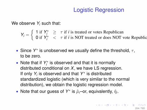
Logistic Regression
We observe Yi such that:
Yi =
1 if Y ∗i ≥ τ if i is treated or votes Republican0 if Y ∗i < τ if i is NOT treated or does NOT vote Republican
• Since Y ∗ is unobserved we usually define the threshold, τ ,to be zero.
• Note that if Y ∗i is observed and that it is normallydistributed conditional on X , we have LS regression.If only Yi is observed and that Y ∗ is distributedstandardized logistic (which is very similar to the normaldistribution), we obtain the logistic regression model.
• Note that our guess of Y ∗ is µi–or, equivalently, ηi .
204 / 765
Logistic Regression Coefficients
• The estimated coefficients, β, in a logistic regression canbe interpreted in a manner very similar to that thecoefficients in LS. But there are important differenceswhich complicate the issue.
• We should interpret β as the regression coefficients of Y ∗
on X . So, β1 is what happens to Y ∗i when X1 goes up byone unit when all of the other explanatory variables remainthe same. ICK! Causal
• The interpretation is complicated by the fact that the linkfunction is nonlinear. So the effect of a one unit change inX1 on the predicted probability is different if the otherexplanatory variables are held at one given constant valueversus another. Why is this?
205 / 765
Logistic Regression Assumptions andProperties
• The assumptions of logistic regression are very similar tothose of least squares—see the assumptions slide. Butthere are some important difference. The most important isthat in order to obtain consistency, logistic regressionrequires the homoscedasticity assumption while LS doesnot.
• We also need the no perfect separation assumption for theexistence of the estimator.
• Another important difference is that logistic regression isNOT unbiased. But it is consistent.
206 / 765
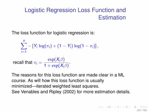
Logistic Regression Loss Function andEstimation
The loss function for logistic regression is:
n∑i=1
− [Yi log(πi) + (1− Yi) log(1− πi)] ,
recall that πi =exp(Xiβ)
1 + exp(Xiβ).
The reasons for this loss function are made clear in a MLcourse. As will how this loss function is usuallyminimized—iterated weighted least squares.See Venables and Ripley (2002) for more estimation details.
207 / 765
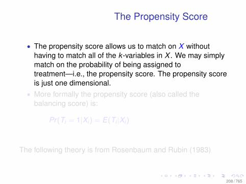
The Propensity Score
• The propensity score allows us to match on X withouthaving to match all of the k -variables in X . We may simplymatch on the probability of being assigned totreatment—i.e., the propensity score. The propensity scoreis just one dimensional.
• More formally the propensity score (also called thebalancing score) is:
Pr(Ti = 1|Xi) = E(Ti |Xi)
The following theory is from Rosenbaum and Rubin (1983)
208 / 765
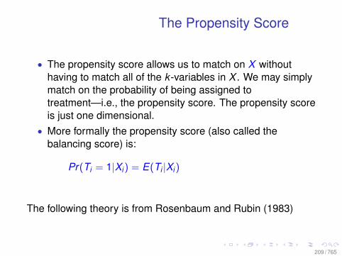
The Propensity Score
• The propensity score allows us to match on X withouthaving to match all of the k -variables in X . We may simplymatch on the probability of being assigned totreatment—i.e., the propensity score. The propensity scoreis just one dimensional.
• More formally the propensity score (also called thebalancing score) is:
Pr(Ti = 1|Xi) = E(Ti |Xi)
The following theory is from Rosenbaum and Rubin (1983)
209 / 765
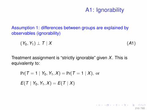
A1: Ignorability
Assumption 1: differences between groups are explained byobservables (ignorability)
(Y0,Y1) ⊥ T | X (A1)
Treatment assignment is “strictly ignorable” given X . This isequivalenty to:
Pr(T = 1 | Y0,Y1,X ) = Pr(T = 1 | X ), or
E(T | Y0,Y1,X ) = E(T | X )
210 / 765
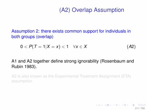
(A2) Overlap Assumption
Assumption 2: there exists common support for individuals inboth groups (overlap)
0 < P(T = 1|X = x) < 1 ∀x ∈ X (A2)
A1 and A2 together define strong ignorability (Rosenbaum andRubin 1983).
A2 is also known as the Experimental Treatment Assignment (ETA)assumption
211 / 765
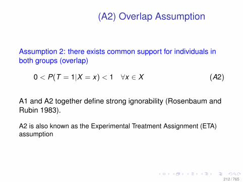
(A2) Overlap Assumption
Assumption 2: there exists common support for individuals inboth groups (overlap)
0 < P(T = 1|X = x) < 1 ∀x ∈ X (A2)
A1 and A2 together define strong ignorability (Rosenbaum andRubin 1983).
A2 is also known as the Experimental Treatment Assignment (ETA)assumption
212 / 765
Observabled Quantities
We observe the conditional distributions:• F (Y1 | X ,T = 1) and• F (Y0 | X ,T = 0)
But not the joint distributions:• F (Y0,Y1 | X ,T = 1)
• F (Y0,Y1 | X )
Nor the impact distrubtion:• F (Y1 − Y0 | X ,T = 1)
213 / 765
Weaker Assumptions
For ATT, weaker assumptions can be made:• A weaker conditional mean independence assumption on
Y0 is sufficient (Heckman, Ichimura, and Todd 1998).
E(Y0 | X ,T = 1) = E(Y0 | X ,T = 0) = E(Y0 | X )
• A weaker support condition:
Pr(T = 1 | X ) < 1
This is sufficient because we only need to guarantee acontrol analogue for every treatment, and not the reverse
214 / 765
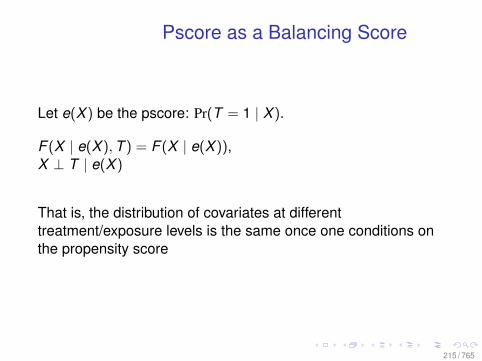
Pscore as a Balancing Score
Let e(X ) be the pscore: Pr(T = 1 | X ).
F (X | e(X ),T ) = F (X | e(X )),X ⊥ T | e(X )
That is, the distribution of covariates at differenttreatment/exposure levels is the same once one conditions onthe propensity score
215 / 765

Balancing Score: intuition
We wish to show that if one matches on the true propensity score,asymptotically, the observed covariates, X , will be balanced betweentreatment and control groups. Assume that conditioning on the truepropensity score does not balance the underlying X covariates. Thenthere exists x1 and x2 such that e(X1) = e(X2), so that conditioning one(X ), still results in imbalance of x1 and x2. Imbalance by definitionimplies that Pr(Ti = 1 | x1) 6= Pr(Ti = 1 | x2), but this contradictse(x1) = e(x2) since by the definition of the propensity score:
e(x1) = Pr(Ti = 1 | x1), ande(x2) = Pr(Ti = 1 | x2).
Therefore, the observed covariates X must be balanced afterconditioning on the true propensity score. For details:P. R. Rosenbaum and Rubin (1983), especially theorems 1–3.
216 / 765
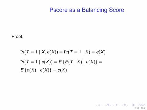
Pscore as a Balancing Score
Proof:
Pr(T = 1 | X ,e(X )) = Pr(T = 1 | X ) = e(X )
Pr(T = 1 | e(X )) = E E(T | X ) | e(X ) =
E e(X ) | e(X ) = e(X )
217 / 765
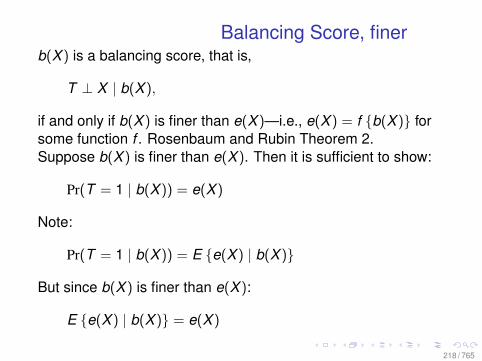
Balancing Score, finerb(X ) is a balancing score, that is,
T ⊥ X | b(X ),
if and only if b(X ) is finer than e(X )—i.e., e(X ) = f b(X ) forsome function f . Rosenbaum and Rubin Theorem 2.Suppose b(X ) is finer than e(X ). Then it is sufficient to show:
Pr(T = 1 | b(X )) = e(X )
Note:
Pr(T = 1 | b(X )) = E e(X ) | b(X )
But since b(X ) is finer than e(X ):
E e(X ) | b(X ) = e(X )
218 / 765
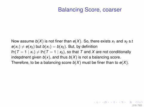
Balancing Score, coarser
Now assume b(X ) is not finer than e(X ). So, there exists x1 and x2 s.te(x1) 6= e(x2) but b(x1) = b(x2). But, by definitionPr(T = 1 | x1) 6= Pr(T = 1 | x2), so that T and X are not conditionallyindepdnent given b(x), and thus b(X ) is not a balancing score.Therefore, to be a balancing score b(X ) must be finer than to e(X ).
219 / 765
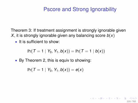
Pscore and Strong Ignorability
Theorem 3: If treatment assignment is strongly ignorable givenX , it is strongly ignorable given any balancing score b(x)
• It is sufficient to show:
Pr(T = 1 | Y0,Y1,b(x)) = Pr(T = 1 | b(x))
• By Theorem 2, this is equiv to showing:
Pr(T = 1 | Y0,Y1,b(x)) = e(x)
220 / 765
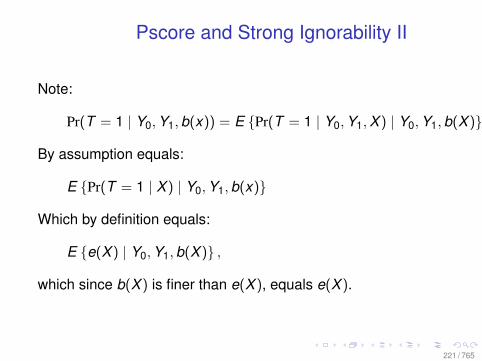
Pscore and Strong Ignorability II
Note:
Pr(T = 1 | Y0,Y1,b(x)) = E Pr(T = 1 | Y0,Y1,X ) | Y0,Y1,b(X )
By assumption equals:
E Pr(T = 1 | X ) | Y0,Y1,b(x)
Which by definition equals:
E e(X ) | Y0,Y1,b(X ) ,
which since b(X ) is finer than e(X ), equals e(X ).
221 / 765
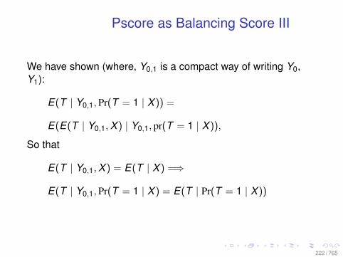
Pscore as Balancing Score III
We have shown (where, Y0,1 is a compact way of writing Y0,Y1):
E(T | Y0,1,Pr(T = 1 | X )) =
E(E(T | Y0,1,X ) | Y0,1, pr(T = 1 | X )),
So that
E(T | Y0,1,X ) = E(T | X ) =⇒
E(T | Y0,1,Pr(T = 1 | X ) = E(T | Pr(T = 1 | X ))
222 / 765
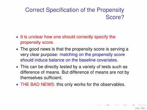
Correct Specification of the PropensityScore?
• It is unclear how one should correctly specify thepropensity score.
• The good news is that the propensity score is serving avery clear purpose: matching on the propensity scoreshould induce balance on the baseline covariates.
• This can be directly tested by a variety of tests such asdifference of means. But difference of means are not bythemselves sufficient.
• THE BAD NEWS: this only works for the observables.
223 / 765
Estimating the Propensity Score
• We we may estimate the propensity score using logisticregression where the treatment indicator is the dependentvariable.
• We then match on either the predicted probabilities πi orthe linear predictor ηi . It is in fact preferable to match on thelinear predictor because the probabilities are compressed.
• For matching, we do not care about the parameters, β. Weonly care about getting good estimates of πi .
224 / 765
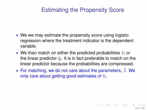
Estimating the Propensity Score
• We we may estimate the propensity score using logisticregression where the treatment indicator is the dependentvariable.
• We then match on either the predicted probabilities πi orthe linear predictor ηi . It is in fact preferable to match on thelinear predictor because the probabilities are compressed.
• For matching, we do not care about the parameters, β. Weonly care about getting good estimates of πi .
225 / 765
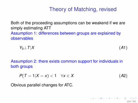
Theory of Matching, revised
Both of the proceeding assumptions can be weakend if we aresimply estimating ATTAssumption 1: differences between groups are explained byobservables
Y0⊥T |X (A1)
Assumption 2: there exists common support for individuals inboth groups
P(T = 1|X = x) < 1 ∀x ∈ X (A2)
Obvious parallel changes for ATC.
226 / 765
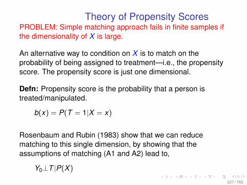
Theory of Propensity ScoresPROBLEM: Simple matching approach fails in finite samples ifthe dimensionality of X is large.
An alternative way to condition on X is to match on theprobability of being assigned to treatment—i.e., the propensityscore. The propensity score is just one dimensional.
Defn: Propensity score is the probability that a person istreated/manipulated.
b(x) = P(T = 1|X = x)
Rosenbaum and Rubin (1983) show that we can reducematching to this single dimension, by showing that theassumptions of matching (A1 and A2) lead to,
Y0⊥T |P(X )
227 / 765
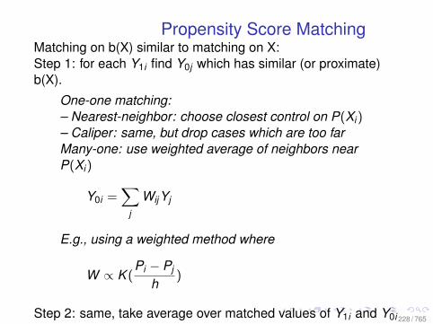
Propensity Score MatchingMatching on b(X) similar to matching on X:Step 1: for each Y1i find Y0j which has similar (or proximate)b(X).
One-one matching:– Nearest-neighbor: choose closest control on P(Xi)– Caliper: same, but drop cases which are too farMany-one: use weighted average of neighbors nearP(Xi)
Y0i =∑
j
WijYj
E.g., using a weighted method where
W ∝ K (Pi − Pj
h)
Step 2: same, take average over matched values of Y1i and Y0i 228 / 765
Properties of Pscore Matching I
• The modeling portion of the estimator is limited to themodel of p(Xi). Estimation of this model requires noknowledge of the outcome.
• Unlike in the regression case, there is a clear standard forchoosing an optimal model; it is the model which balancesthe covariates, X .
• The key assumption required is that no variable has beenleft unobserved which is correlated with treatmentassignment and with the outcome. This is called theselection on observables assumption.
229 / 765
Properties of Pscore Matching I
• The modeling portion of the estimator is limited to themodel of p(Xi). Estimation of this model requires noknowledge of the outcome.
• Unlike in the regression case, there is a clear standard forchoosing an optimal model; it is the model which balancesthe covariates, X .
• The key assumption required is that no variable has beenleft unobserved which is correlated with treatmentassignment and with the outcome. This is called theselection on observables assumption.
230 / 765
Properties of Pscore Matching I
• The modeling portion of the estimator is limited to themodel of p(Xi). Estimation of this model requires noknowledge of the outcome.
• Unlike in the regression case, there is a clear standard forchoosing an optimal model; it is the model which balancesthe covariates, X .
• The key assumption required is that no variable has beenleft unobserved which is correlated with treatmentassignment and with the outcome. This is called theselection on observables assumption.
231 / 765
Properties of Pscore Matching II
• No functional form is implied for the relationship betweentreatment and outcome. No homogeneous causal effectassumption has been made.
• Since we are interested in a lower dimensionalrepresentation of Xi , in particular p(Xi), we do not need toestimate consistently any of the individual parameters inour propensity model—they don’t even need to beidentified.
232 / 765
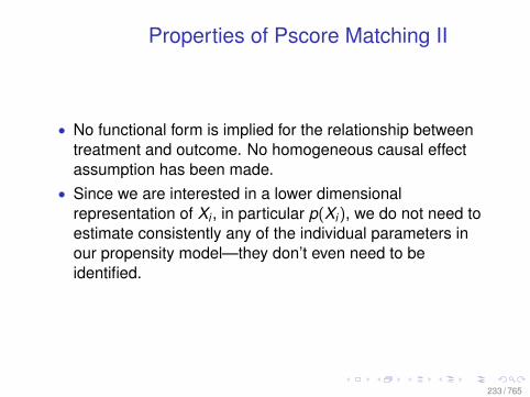
Properties of Pscore Matching II
• No functional form is implied for the relationship betweentreatment and outcome. No homogeneous causal effectassumption has been made.
• Since we are interested in a lower dimensionalrepresentation of Xi , in particular p(Xi), we do not need toestimate consistently any of the individual parameters inour propensity model—they don’t even need to beidentified.
233 / 765
Properties of Pscore Matching III
• Because we are taking a conditional expectation, we needto decide what to condition on. If we condition too little, wedo not obtain strong ignorability. If we condition onvariables which are not baseline variables, we also obtainbiased estimates.
234 / 765
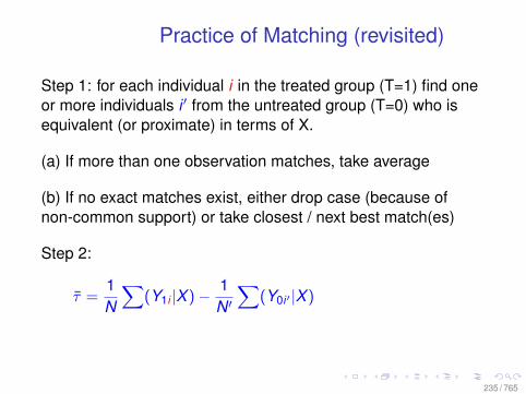
Practice of Matching (revisited)
Step 1: for each individual i in the treated group (T=1) find oneor more individuals i ′ from the untreated group (T=0) who isequivalent (or proximate) in terms of X.
(a) If more than one observation matches, take average
(b) If no exact matches exist, either drop case (because ofnon-common support) or take closest / next best match(es)
Step 2:
τ =1N
∑(Y1i |X )− 1
N ′∑
(Y0i ′ |X )
235 / 765
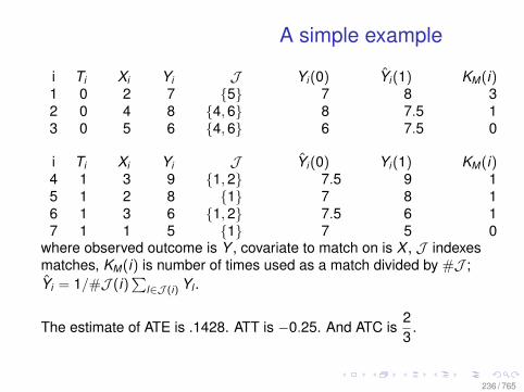
A simple example
i Ti Xi Yi J Yi (0) Yi (1) KM(i)1 0 2 7 5 7 8 32 0 4 8 4,6 8 7.5 13 0 5 6 4,6 6 7.5 0
i Ti Xi Yi J Yi (0) Yi (1) KM(i)4 1 3 9 1,2 7.5 9 15 1 2 8 1 7 8 16 1 3 6 1,2 7.5 6 17 1 1 5 1 7 5 0
where observed outcome is Y , covariate to match on is X , J indexesmatches, KM(i) is number of times used as a match divided by #J ;Yi = 1/#J (i)
∑l∈J (i) Yl .
The estimate of ATE is .1428. ATT is −0.25. And ATC is23
.
236 / 765
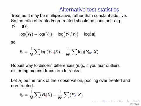
Alternative test statisticsTreatment may be multiplicative, rather than constant additive.So the ratio of treated/non-treated should be constant: e.g.,Y1 = aY0
log(Y1)− log(Y0) = log(Y1/Y0) = log(a)
so,
τ2 =1N
∑log(Y1i |X )− 1
N ′∑
log(Y0i ′ |X )
Robust way to discern differences (e.g., if you fear outliersdistorting means) transform to ranks:
Let Ri be the rank of the i observation, pooling over treated andnon-treated.
τ3 =1N
∑(Ri |X )− 1
N ′∑
(Ri ′ |X )
237 / 765
Comments
• If you think the variances are changed by treatment, butnot the location, then test differences in variances.
• The point: your test statistic should be motivated by yourtheory of what is changing when manipulation / treatmentoccurs!
• One could in theory estimate any model one wishes on thematched data. Such as regression, logistic regression etc.
238 / 765
RDD Readings• Lee, D., 2008. “Randomized experiments from non-random
selection in U.S. house elections.” Journal of Econometrics142:2 675–697.
• Devin Caughey and Jasjeet S. Sekhon. “Elections and theRegression-Discontinuity Design: Lessons from Close U.S.House Races, 1942–2008.” Political Analysis. 19 (4): 385–408.2011.
• Thistlethwaite, D. and D. Campbell. 1960.“Regression-Discontinuity Analysis: An alternative to the ex postfacto experiment.” Journal of Educational Psychology 51 (6):309–317.
• Gerber, Alan S. and Donald P. Green. “Field Experiments andNatural Experiments.” Oxford Handbook of PoliticalMethodology.
• Hahn J., P. Todd, and W.V. der Klaauw, 2001. “Identification andEstimation of Treatment Effects with a Regression-DiscontinuityDesign.” Econometrica.
239 / 765
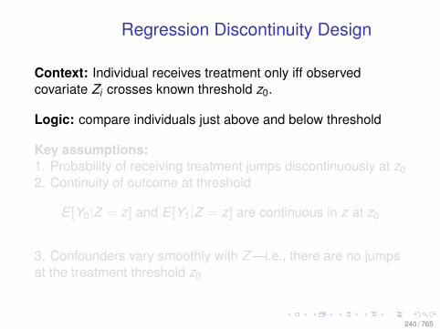
Regression Discontinuity Design
Context: Individual receives treatment only iff observedcovariate Zi crosses known threshold z0.
Logic: compare individuals just above and below threshold
Key assumptions:1. Probability of receiving treatment jumps discontinuously at z02. Continuity of outcome at threshold
E [Y0|Z = z] and E [Y1|Z = z] are continuous in z at z0
3. Confounders vary smoothly with Z—i.e., there are no jumpsat the treatment threshold z0
240 / 765
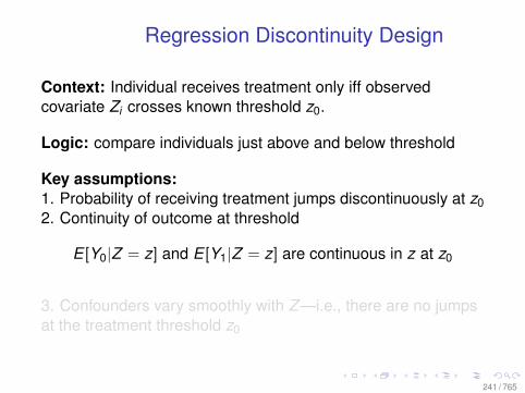
Regression Discontinuity Design
Context: Individual receives treatment only iff observedcovariate Zi crosses known threshold z0.
Logic: compare individuals just above and below threshold
Key assumptions:1. Probability of receiving treatment jumps discontinuously at z02. Continuity of outcome at threshold
E [Y0|Z = z] and E [Y1|Z = z] are continuous in z at z0
3. Confounders vary smoothly with Z—i.e., there are no jumpsat the treatment threshold z0
241 / 765
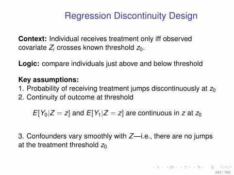
Regression Discontinuity Design
Context: Individual receives treatment only iff observedcovariate Zi crosses known threshold z0.
Logic: compare individuals just above and below threshold
Key assumptions:1. Probability of receiving treatment jumps discontinuously at z02. Continuity of outcome at threshold
E [Y0|Z = z] and E [Y1|Z = z] are continuous in z at z0
3. Confounders vary smoothly with Z—i.e., there are no jumpsat the treatment threshold z0
242 / 765
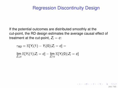
Regression Discontinuity Design
If the potential outcomes are distributed smoothly at thecut-point, the RD design estimates the average causal effect oftreatment at the cut-point, Zi = c:
τRD ≡ E[Yi(1)− Yi(0)|Zi = c] =
limZi↓c
E[Yi(1)|Zi = c]− limZi↑c
E[Yi(0)|Zi = c]
243 / 765
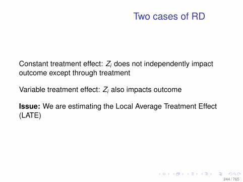
Two cases of RD
Constant treatment effect: Zi does not independently impactoutcome except through treatment
Variable treatment effect: Zi also impacts outcome
Issue: We are estimating the Local Average Treatment Effect(LATE)
244 / 765
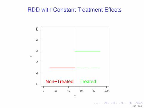
RDD with Constant Treatment Effects
0 20 40 60 80 100
020
4060
8010
0
Z
Y
Non−Treated Treated
245 / 765
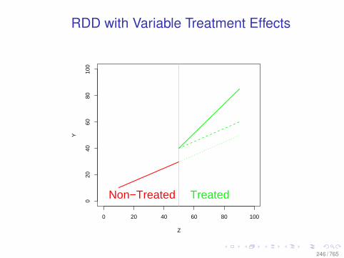
RDD with Variable Treatment Effects
0 20 40 60 80 100
020
4060
8010
0
Z
Y
Non−Treated Treated
246 / 765
Example 1: Scholarship Winners
• From Kenya to the U.S. RDD has been used to estimatethe effect of school scholarships.
• In these cases, z is the measure of academic performancewhich determines if one receives a scholarship—e.g., testscores, GPA.
• Of course, comparing everyone who wins a scholarshipwith everyone who loses is not a good way to proceed.
• Focus attention on people who just won and who just lost.• This reduces omitted variable/selection bais, why?
247 / 765
RDD and Omitted Variable Bias I
• Let’s assume that there is a homogeneous causal effect:Yi = α + βTi + γXi + εi ,
where T is the treatment indicator and X is a confounder.• Then:
E(Yi | Ti = 1)− E(Yi | Ti = 0)
= [α + β + γE(Xi | Ti = 1) + E(εi | Ti = 1)]
− [α + 0 + γE(Xi | Ti = 0) + E(εi | Ti = 0)]
= β + γ [E(Xi | Ti = 1)− E(Xi | Ti = 0)]
True Effect + Bias
248 / 765
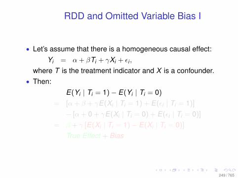
RDD and Omitted Variable Bias I
• Let’s assume that there is a homogeneous causal effect:Yi = α + βTi + γXi + εi ,
where T is the treatment indicator and X is a confounder.• Then:
E(Yi | Ti = 1)− E(Yi | Ti = 0)
= [α + β + γE(Xi | Ti = 1) + E(εi | Ti = 1)]
− [α + 0 + γE(Xi | Ti = 0) + E(εi | Ti = 0)]
= β + γ [E(Xi | Ti = 1)− E(Xi | Ti = 0)]
True Effect + Bias
249 / 765
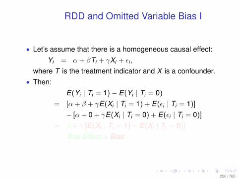
RDD and Omitted Variable Bias I
• Let’s assume that there is a homogeneous causal effect:Yi = α + βTi + γXi + εi ,
where T is the treatment indicator and X is a confounder.• Then:
E(Yi | Ti = 1)− E(Yi | Ti = 0)
= [α + β + γE(Xi | Ti = 1) + E(εi | Ti = 1)]
− [α + 0 + γE(Xi | Ti = 0) + E(εi | Ti = 0)]
= β + γ [E(Xi | Ti = 1)− E(Xi | Ti = 0)]
True Effect + Bias
250 / 765
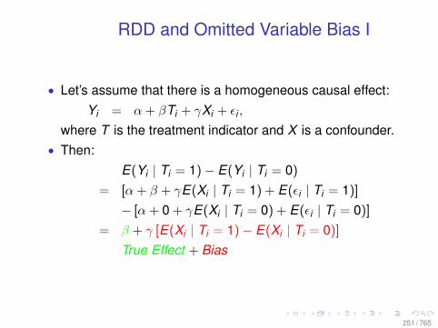
RDD and Omitted Variable Bias I
• Let’s assume that there is a homogeneous causal effect:Yi = α + βTi + γXi + εi ,
where T is the treatment indicator and X is a confounder.• Then:
E(Yi | Ti = 1)− E(Yi | Ti = 0)
= [α + β + γE(Xi | Ti = 1) + E(εi | Ti = 1)]
− [α + 0 + γE(Xi | Ti = 0) + E(εi | Ti = 0)]
= β + γ [E(Xi | Ti = 1)− E(Xi | Ti = 0)]
True Effect + Bias
251 / 765
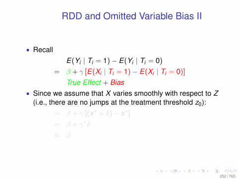
RDD and Omitted Variable Bias II
• RecallE(Yi | Ti = 1)− E(Yi | Ti = 0)
= β + γ [E(Xi | Ti = 1)− E(Xi | Ti = 0)]
True Effect + Bias• Since we assume that X varies smoothly with respect to Z
(i.e., there are no jumps at the treatment threshold z0):= β + γ [(x∗ + δ)− x∗]= β + γ∗δ
≈ β
252 / 765
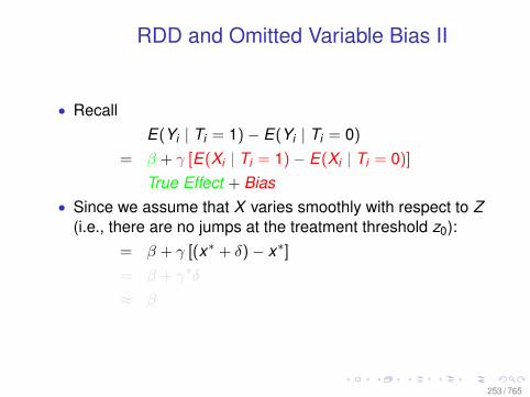
RDD and Omitted Variable Bias II
• RecallE(Yi | Ti = 1)− E(Yi | Ti = 0)
= β + γ [E(Xi | Ti = 1)− E(Xi | Ti = 0)]
True Effect + Bias• Since we assume that X varies smoothly with respect to Z
(i.e., there are no jumps at the treatment threshold z0):= β + γ [(x∗ + δ)− x∗]= β + γ∗δ
≈ β
253 / 765
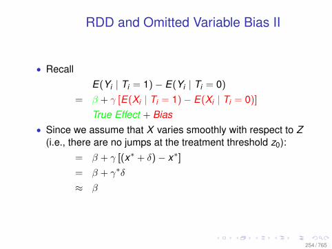
RDD and Omitted Variable Bias II
• RecallE(Yi | Ti = 1)− E(Yi | Ti = 0)
= β + γ [E(Xi | Ti = 1)− E(Xi | Ti = 0)]
True Effect + Bias• Since we assume that X varies smoothly with respect to Z
(i.e., there are no jumps at the treatment threshold z0):= β + γ [(x∗ + δ)− x∗]= β + γ∗δ
≈ β
254 / 765
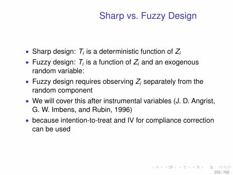
Sharp vs. Fuzzy Design
• Sharp design: Ti is a deterministic function of Zi
• Fuzzy design: Ti is a function of Zi and an exogenousrandom variable:
• Fuzzy design requires observing Zi separately from therandom component
• We will cover this after instrumental variables (J. D. Angrist,G. W. Imbens, and Rubin, 1996)
• because intention-to-treat and IV for compliance correctioncan be used
255 / 765
Incumbency Advantage (IA)
• The Personal Incumbency Advantage is the candidatespecific advantage that results from the benefits of officeholding—e.g:• name recognition; incumbency cue• constituency service• public position taking• providing pork
• The Incumbent Party Advantage:• ceteris paribus, voters have a preference for remaining with
the same party they had before• parties have organizational advantages in some districts
256 / 765
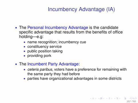
Incumbency Advantage (IA)
• The Personal Incumbency Advantage is the candidatespecific advantage that results from the benefits of officeholding—e.g:• name recognition; incumbency cue• constituency service• public position taking• providing pork
• The Incumbent Party Advantage:• ceteris paribus, voters have a preference for remaining with
the same party they had before• parties have organizational advantages in some districts
257 / 765
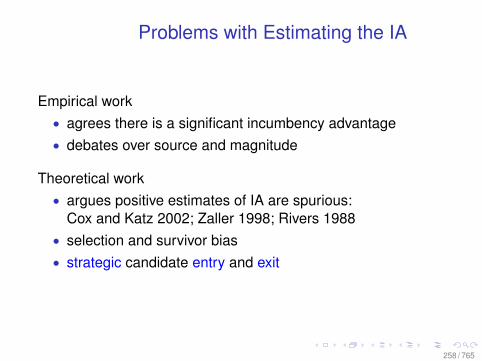
Problems with Estimating the IA
Empirical work• agrees there is a significant incumbency advantage• debates over source and magnitude
Theoretical work• argues positive estimates of IA are spurious:
Cox and Katz 2002; Zaller 1998; Rivers 1988• selection and survivor bias• strategic candidate entry and exit
258 / 765
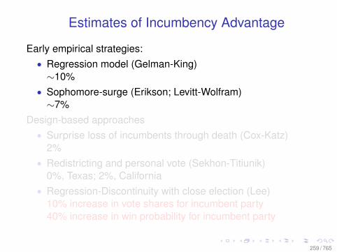
Estimates of Incumbency Advantage
Early empirical strategies:• Regression model (Gelman-King)∼10%
• Sophomore-surge (Erikson; Levitt-Wolfram)∼7%
Design-based approaches• Surprise loss of incumbents through death (Cox-Katz)
2%• Redistricting and personal vote (Sekhon-Titiunik)
0%, Texas; 2%, California• Regression-Discontinuity with close election (Lee)
10% increase in vote shares for incumbent party40% increase in win probability for incumbent party
259 / 765
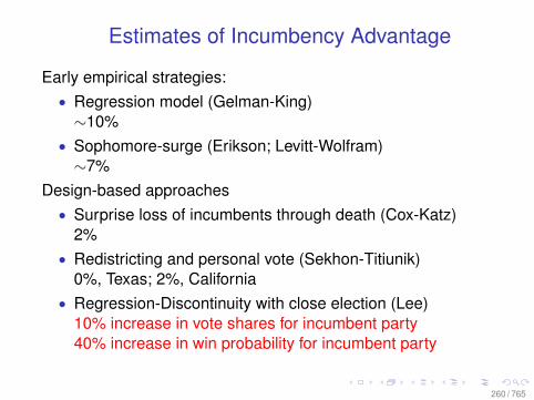
Estimates of Incumbency Advantage
Early empirical strategies:• Regression model (Gelman-King)∼10%
• Sophomore-surge (Erikson; Levitt-Wolfram)∼7%
Design-based approaches• Surprise loss of incumbents through death (Cox-Katz)
2%• Redistricting and personal vote (Sekhon-Titiunik)
0%, Texas; 2%, California• Regression-Discontinuity with close election (Lee)
10% increase in vote shares for incumbent party40% increase in win probability for incumbent party
260 / 765
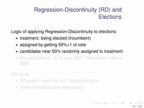
Regression-Discontinuity (RD) andElections
Logic of applying Regression-Discontinuity to elections• treatment: being elected (incumbent)• assigned by getting 50%+1 of vote• candidates near 50% randomly assigned to treatment• first applications: D. S. Lee, 2001, Pettersson-Lidbom,
2001
We show• RD doesn’t work for U.S. House elections• there are substantive implications
261 / 765
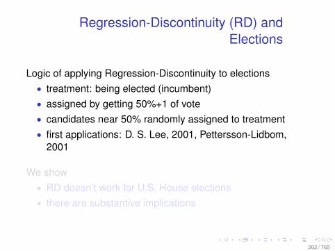
Regression-Discontinuity (RD) andElections
Logic of applying Regression-Discontinuity to elections• treatment: being elected (incumbent)• assigned by getting 50%+1 of vote• candidates near 50% randomly assigned to treatment• first applications: D. S. Lee, 2001, Pettersson-Lidbom,
2001
We show• RD doesn’t work for U.S. House elections• there are substantive implications
262 / 765
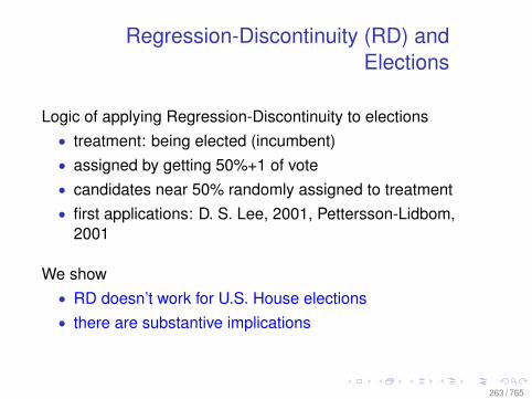
Regression-Discontinuity (RD) andElections
Logic of applying Regression-Discontinuity to elections• treatment: being elected (incumbent)• assigned by getting 50%+1 of vote• candidates near 50% randomly assigned to treatment• first applications: D. S. Lee, 2001, Pettersson-Lidbom,
2001
We show• RD doesn’t work for U.S. House elections• there are substantive implications
263 / 765
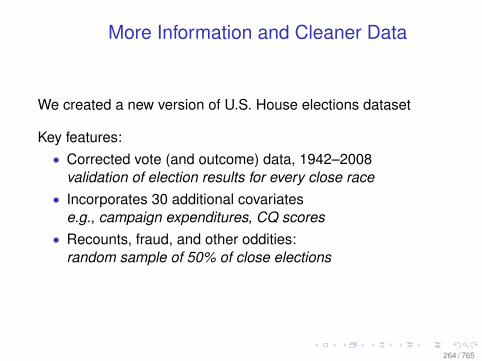
More Information and Cleaner Data
We created a new version of U.S. House elections dataset
Key features:• Corrected vote (and outcome) data, 1942–2008
validation of election results for every close race• Incorporates 30 additional covariates
e.g., campaign expenditures, CQ scores• Recounts, fraud, and other oddities:
random sample of 50% of close elections
264 / 765
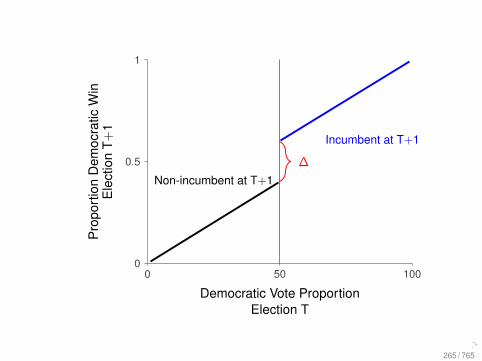
Non-incumbent at T+1
Incumbent at T+1
∆
0 50 1000
0.5
1
Democratic Vote ProportionElection T
Pro
port
ion
Dem
ocra
ticW
inE
lect
ion
T+1
265 / 765
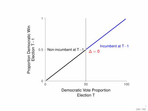
Non-incumbent at T−1Incumbent at T−1
∆ = 0
0 50 1000
0.5
1
Democratic Vote ProportionElection T
Pro
port
ion
Dem
ocra
ticW
inE
lect
ion
T−1
266 / 765
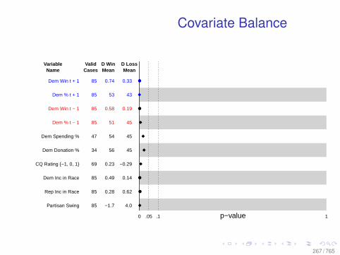
Covariate Balance
VariableName
ValidCases
D WinMean
D LossMean
Dem Win t − 1 85 0.58 0.19
Dem % t − 1 85 51 45
Dem Spending % 47 54 45
Dem Donation % 34 56 45
CQ Rating −1, 0, 1 69 0.23 −0.29
Dem Inc in Race 85 0.49 0.14
Rep Inc in Race 85 0.28 0.62
Partisan Swing 85 −1.7 4.0
Dem Win t + 1 85 0.74 0.33
Dem % t + 1 85 53 43
0 .05 .1 1p−value
267 / 765
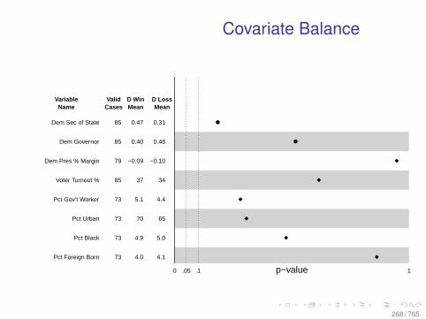
Covariate Balance
VariableName
ValidCases
D WinMean
D LossMean
Dem Sec of State 85 0.47 0.31
Dem Governor 85 0.40 0.48
Dem Pres % Margin 79 −0.09 −0.10
Voter Turnout % 85 37 34
Pct Gov't Worker 73 5.1 4.4
Pct Urban 73 70 65
Pct Black 73 4.9 5.0
Pct Foreign Born 73 4.0 4.1
0 .05 .1 1p−value
268 / 765
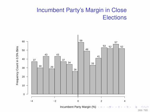
Incumbent Party’s Margin in CloseElections
Incumbent Party Margin (%)
Fre
quen
cy C
ount
in 0
.5%
Bin
s
−4 −2 0 2 4
0
10
20
30
40
50
60
37
30
43
29
43
3734
26
59
49
33
41
53 52
57
52
269 / 765
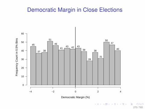
Democratic Margin in Close Elections
Democratic Margin (%)
Fre
quen
cy C
ount
in 0
.5%
Bin
s
−4 −2 0 2 4
0
10
20
30
40
50
60
45
37 38
51
46
4143 42 43
39
28
38
31
5047
40
270 / 765
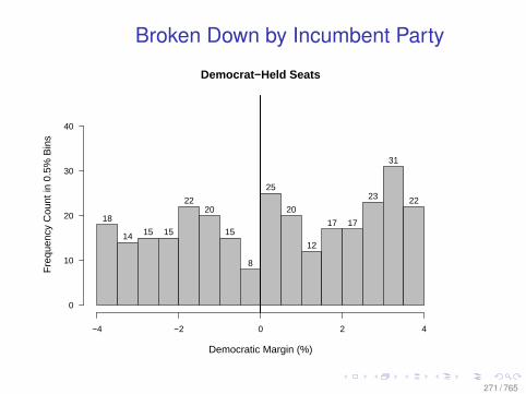
Broken Down by Incumbent Party
Democrat−Held Seats
Democratic Margin (%)
Fre
quen
cy C
ount
in 0
.5%
Bin
s
−4 −2 0 2 4
0
10
20
30
40
18
14 15 15
2220
15
8
25
20
12
17 17
23
31
22
271 / 765
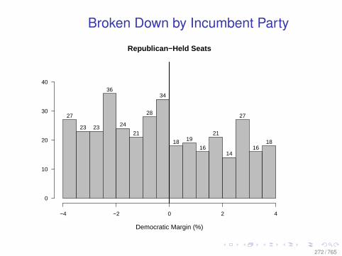
Broken Down by Incumbent Party
Republican−Held Seats
Democratic Margin (%)
−4 −2 0 2 4
0
10
20
30
40
27
23 23
36
24
21
28
34
18 19
16
21
14
27
1618
272 / 765
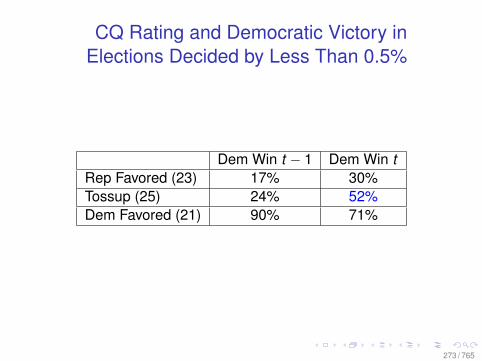
CQ Rating and Democratic Victory inElections Decided by Less Than 0.5%
Dem Win t − 1 Dem Win tRep Favored (23) 17% 30%Tossup (25) 24% 52%Dem Favored (21) 90% 71%
273 / 765
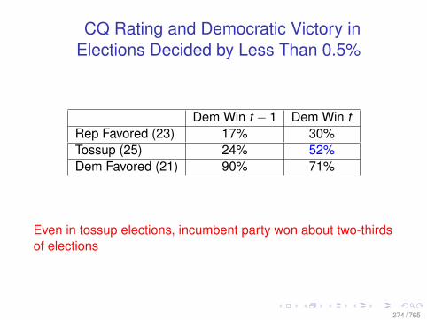
CQ Rating and Democratic Victory inElections Decided by Less Than 0.5%
Dem Win t − 1 Dem Win tRep Favored (23) 17% 30%Tossup (25) 24% 52%Dem Favored (21) 90% 71%
Even in tossup elections, incumbent party won about two-thirdsof elections
274 / 765
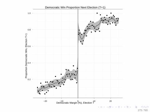
Democratic Win Proportion Next Election (T+1)
Democratic Margin (%), Election T
Pro
port
ion
Dem
ocra
tic W
in, E
lect
ion
T+
1
0.2
0.4
0.6
0.8
1.0
−20 −10 0 10 20
275 / 765
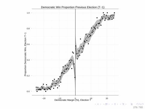
Democratic Win Proportion Previous Election (T−1)
Democratic Margin (%), Election T
Pro
port
ion
Dem
ocra
tic W
in, E
lect
ion
T−
1
0.0
0.2
0.4
0.6
0.8
1.0
−20 −10 0 10 20
276 / 765
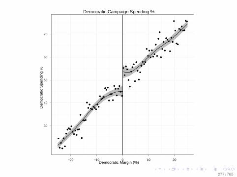
Democratic Campaign Spending %
Democratic Margin (%)
Dem
ocra
tic S
pend
ing
%
30
40
50
60
70
−20 −10 0 10 20
277 / 765
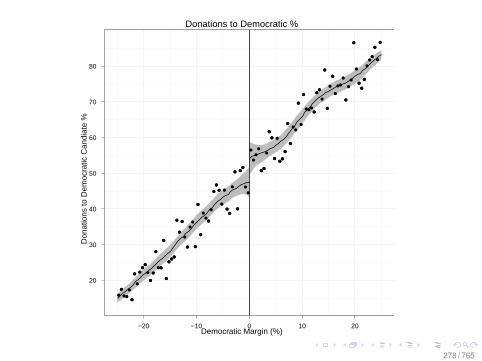
Donations to Democratic %
Democratic Margin (%)
Don
atio
ns to
Dem
ocra
tic C
andi
ate
%
20
30
40
50
60
70
80
−20 −10 0 10 20
278 / 765
Divergence Figures
The following two figures plot the divergence of covariatedistributions in the immediate neighborhood of the cut-point.Covariate differences are plotted against the mid-point of thedisjoint interval tested (e.g., 1.5 for the interval (−1.75,−1.25),(1.75,1.25). Loess lines highlight the trends in the imbalance.
279 / 765
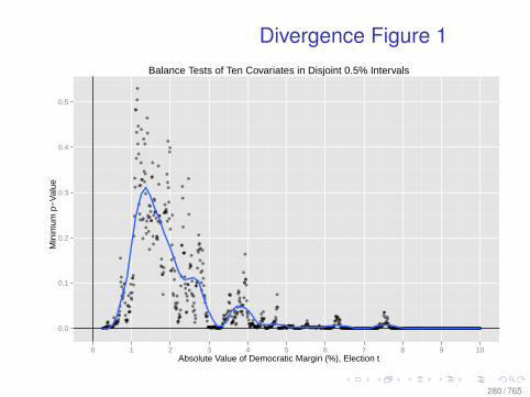
Divergence Figure 1Balance Tests of Ten Covariates in Disjoint 0.5% Intervals
Absolute Value of Democratic Margin (%), Election t
Min
imum
p−
Val
ue
0.0
0.1
0.2
0.3
0.4
0.5
0 1 2 3 4 5 6 7 8 9 10
280 / 765
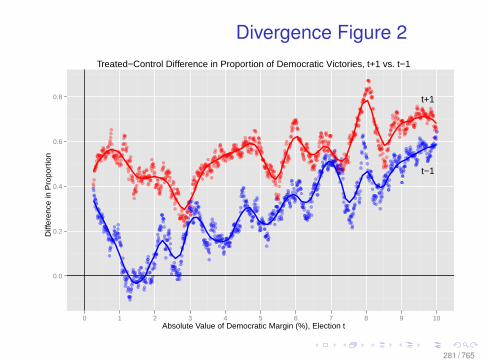
Divergence Figure 2Treated−Control Difference in Proportion of Democratic Victories, t+1 vs. t−1
Absolute Value of Democratic Margin (%), Election t
Diff
eren
ce in
Pro
port
ion
0.0
0.2
0.4
0.6
0.8 t+1
t−1
0 1 2 3 4 5 6 7 8 9 10
281 / 765
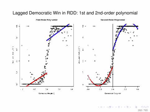
Lagged Democratic Win in RDD: 1st and 2nd-order polynomial
282 / 765
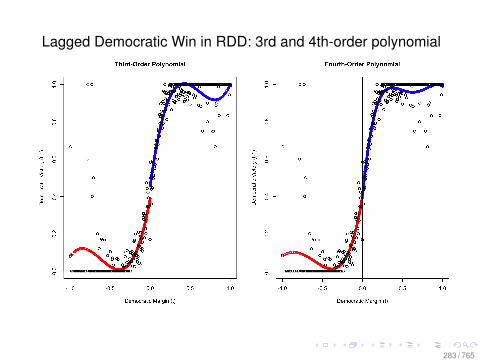
Lagged Democratic Win in RDD: 3rd and 4th-order polynomial
283 / 765

Lagged Democratic Win in RDD: 8th-order polynomial
284 / 765
National Partisan Swings
• Partisan swings are imbalanced:• 1958 (pro-Democratic tide): all 6 close elections occurred
in Republican-held seats• 1994 (pro-Republican tide): all 5 close elections occurred
in Democratic-held seats• Close elections do not generally occur in 50/50 districts
285 / 765
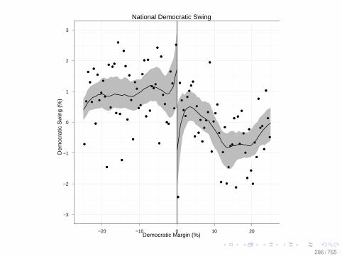
National Democratic Swing
Democratic Margin (%)
Dem
ocra
tic S
win
g (%
)
−3
−2
−1
0
1
2
3
−20 −10 0 10 20
286 / 765
There is Strategic Exit
Strategic exit among incumbents• 20% who barely win retire prior to next election• but all candidates who barely won first election
ran for reelection• even outside of the RD window, previous election margin is
predictive of retirements not due to running for higheroffice:• e.g., 1994: Equal percentage of Republicans and
Democrats retired, but Republicans left to run for higheroffice (13 of 20) Democrats did not (7 of 27)
• 2006: 18 Republican open seats versus 9 Democratic openseats
• 2010: In non-safe seats, 6 Republicans retired, but 15Democrats retired
287 / 765
There is Strategic Exit
Strategic exit among incumbents• 20% who barely win retire prior to next election• but all candidates who barely won first election
ran for reelection• even outside of the RD window, previous election margin is
predictive of retirements not due to running for higheroffice:• e.g., 1994: Equal percentage of Republicans and
Democrats retired, but Republicans left to run for higheroffice (13 of 20) Democrats did not (7 of 27)
• 2006: 18 Republican open seats versus 9 Democratic openseats
• 2010: In non-safe seats, 6 Republicans retired, but 15Democrats retired
288 / 765
There is Strategic Exit
Strategic exit among incumbents• 20% who barely win retire prior to next election• but all candidates who barely won first election
ran for reelection• even outside of the RD window, previous election margin is
predictive of retirements not due to running for higheroffice:• e.g., 1994: Equal percentage of Republicans and
Democrats retired, but Republicans left to run for higheroffice (13 of 20) Democrats did not (7 of 27)
• 2006: 18 Republican open seats versus 9 Democratic openseats
• 2010: In non-safe seats, 6 Republicans retired, but 15Democrats retired
289 / 765
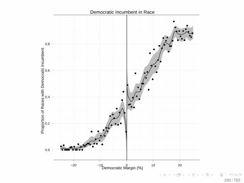
Democratic Incumbent in Race
Democratic Margin (%)
Pro
port
ion
of R
aces
with
Dem
ocra
tic In
cum
bent
0.0
0.2
0.4
0.6
0.8
−20 −10 0 10 20
290 / 765
Money and Incumbents in CloseElections
The imbalances in campaign resources occur because:
• When incumbent candidates run, they have more money:62% of donations and 58% of expenditures
Money isn’t predictive of winning, although they usually win
• In open seats, the incumbent party’s candidates raise 50%of the money but spend 54%
Winners have more money:
winners raise 54% versus 41% (p=0.01)spend 56% versus 49% (p=0.02)
291 / 765
Money and Incumbents in CloseElections
The imbalances in campaign resources occur because:
• When incumbent candidates run, they have more money:62% of donations and 58% of expenditures
Money isn’t predictive of winning, although they usually win
• In open seats, the incumbent party’s candidates raise 50%of the money but spend 54%
Winners have more money:
winners raise 54% versus 41% (p=0.01)spend 56% versus 49% (p=0.02)
292 / 765
Recounts?
New data on close races• for random sample of half of all 130 elections in the
50% + /− 0.75 window• detailed information from news coverage and
administration records on each electionRecounts found in half of the elections (35 recounts)• Imbalance on previous Democratic victory is greater in
recounted elections: a treated-control difference of 0.56versus 0.12
• In the 35 recounted elections, the first election recountwinner was only changed three times
• In each of the three cases, however, the incumbentrepresentative was the ultimate winner
293 / 765
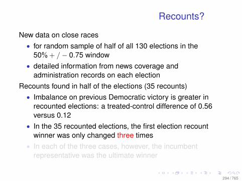
Recounts?
New data on close races• for random sample of half of all 130 elections in the
50% + /− 0.75 window• detailed information from news coverage and
administration records on each electionRecounts found in half of the elections (35 recounts)• Imbalance on previous Democratic victory is greater in
recounted elections: a treated-control difference of 0.56versus 0.12
• In the 35 recounted elections, the first election recountwinner was only changed three times
• In each of the three cases, however, the incumbentrepresentative was the ultimate winner
294 / 765
Recounts?
New data on close races• for random sample of half of all 130 elections in the
50% + /− 0.75 window• detailed information from news coverage and
administration records on each electionRecounts found in half of the elections (35 recounts)• Imbalance on previous Democratic victory is greater in
recounted elections: a treated-control difference of 0.56versus 0.12
• In the 35 recounted elections, the first election recountwinner was only changed three times
• In each of the three cases, however, the incumbentrepresentative was the ultimate winner
295 / 765
Benefits of RD
• Observable implications• Still making weaker assumptions than model based
estimators—e.g., Gelman-King
• Conjecture: RD will work better for elections with lessprofessionalization and where cut point is less known
• Examples of smoothness with RD:• UK: Eggers and Hainmueller (2009)• Brazil: Hidalgo (2010)• California assembly elections• Canadian Parliamentary elections
296 / 765
Benefits of RD
• Observable implications• Still making weaker assumptions than model based
estimators—e.g., Gelman-King
• Conjecture: RD will work better for elections with lessprofessionalization and where cut point is less known
• Examples of smoothness with RD:• UK: Eggers and Hainmueller (2009)• Brazil: Hidalgo (2010)• California assembly elections• Canadian Parliamentary elections
297 / 765
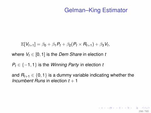
Gelman–King Estimator
E[Vt+1] = β0 + β1Pt + β2(Pt × Rt+1) + β3Vt ,
where Vt ∈ [0,1] is the Dem Share in election t
Pt ∈ −1,1 is the Winning Party in election t
and Rt+1 ∈ 0,1 is a dummy variable indicating whether theIncumbent Runs in election t + 1
298 / 765
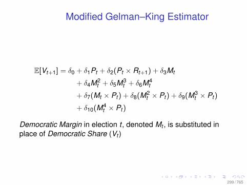
Modified Gelman–King Estimator
E[Vt+1] = δ0 + δ1Pt + δ2(Pt × Rt+1) + δ3Mt
+ δ4M2t + δ5M3
t + δ6M4t
+ δ7(Mt × Pt ) + δ8(M2t × Pt ) + δ9(M3
t × Pt )
+ δ10(M4t × Pt )
Democratic Margin in election t , denoted Mt , is substituted inplace of Democratic Share (Vt )
299 / 765
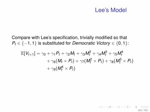
Lee’s Model
Compare with Lee’s specification, trivially modified so thatPt ∈ −1,1 is substituted for Democratic Victory ∈ 0,1:
E[Vt+1] = γ0 + γ1Pt + γ2Mt + γ3M2t + γ4M3
t + γ5M4t
+ γ6(Mt × Pt ) + γ7(M2t × Pt ) + γ8(M3
t × Pt )
+ γ9(M4t × Pt )
300 / 765
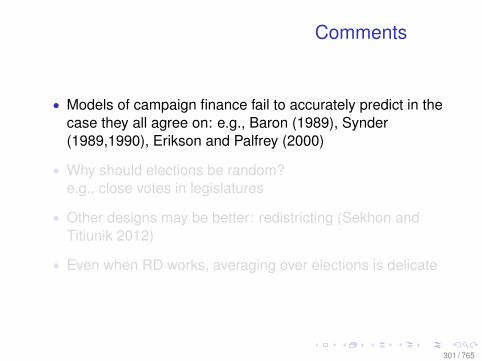
Comments
• Models of campaign finance fail to accurately predict in thecase they all agree on: e.g., Baron (1989), Synder(1989,1990), Erikson and Palfrey (2000)
• Why should elections be random?e.g., close votes in legislatures
• Other designs may be better: redistricting (Sekhon andTitiunik 2012)
• Even when RD works, averaging over elections is delicate
301 / 765
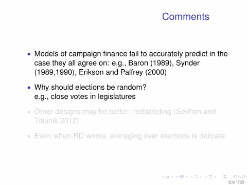
Comments
• Models of campaign finance fail to accurately predict in thecase they all agree on: e.g., Baron (1989), Synder(1989,1990), Erikson and Palfrey (2000)
• Why should elections be random?e.g., close votes in legislatures
• Other designs may be better: redistricting (Sekhon andTitiunik 2012)
• Even when RD works, averaging over elections is delicate
302 / 765
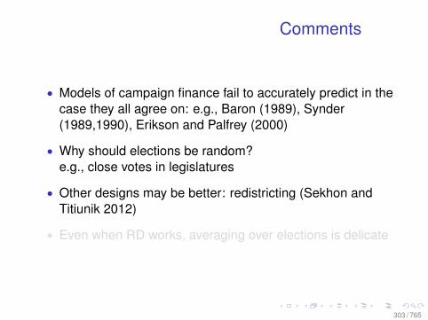
Comments
• Models of campaign finance fail to accurately predict in thecase they all agree on: e.g., Baron (1989), Synder(1989,1990), Erikson and Palfrey (2000)
• Why should elections be random?e.g., close votes in legislatures
• Other designs may be better: redistricting (Sekhon andTitiunik 2012)
• Even when RD works, averaging over elections is delicate
303 / 765
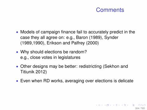
Comments
• Models of campaign finance fail to accurately predict in thecase they all agree on: e.g., Baron (1989), Synder(1989,1990), Erikson and Palfrey (2000)
• Why should elections be random?e.g., close votes in legislatures
• Other designs may be better: redistricting (Sekhon andTitiunik 2012)
• Even when RD works, averaging over elections is delicate
304 / 765
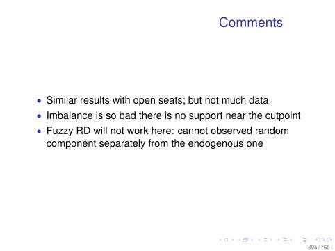
Comments
• Similar results with open seats; but not much data• Imbalance is so bad there is no support near the cutpoint• Fuzzy RD will not work here: cannot observed random
component separately from the endogenous one
305 / 765
Fraud?
• Only few cases of fraud described in secondary literature(e.g., Campbell 2005) also in RD window
• Given the imbalances of resources a priori,fraud isn’t needed as an explanation
306 / 765
Other RD examples to read:
Make sure to read:
Eggers, Andy and Jens Hainmueller. 2009. “The Value ofPolitical Power: Estimating Returns to Office in Post-War BritishPolitics.” American Political Science Review 104(4):513–533.
307 / 765
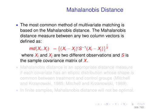
Mahalanobis Distance
• The most common method of multivariate matching isbased on the Mahalanobis distance. The Mahalanobisdistance measure between any two column vectors isdefined as:
md(Xi ,Xj) =
(Xi − Xj)′S−1(Xi − Xj)
12
where Xi and Xj are two different observations and S isthe sample covariance matrix of X .
• Mahalanobis distance is an appropriate distance measureif each covariate has an elliptic distribution whose shape iscommon between treatment and control groups (Mitchelland Krzanowski, 1985; Mitchell and Krzanowski, 1989).
• In finite samples, Mahalanobis distance will not be optimal.
308 / 765
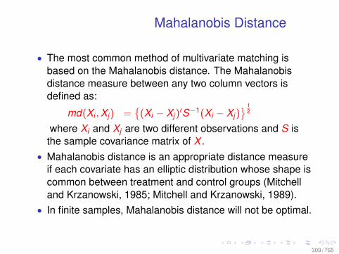
Mahalanobis Distance
• The most common method of multivariate matching isbased on the Mahalanobis distance. The Mahalanobisdistance measure between any two column vectors isdefined as:
md(Xi ,Xj) =
(Xi − Xj)′S−1(Xi − Xj)
12
where Xi and Xj are two different observations and S isthe sample covariance matrix of X .
• Mahalanobis distance is an appropriate distance measureif each covariate has an elliptic distribution whose shape iscommon between treatment and control groups (Mitchelland Krzanowski, 1985; Mitchell and Krzanowski, 1989).
• In finite samples, Mahalanobis distance will not be optimal.
309 / 765
Affine Invariance
• When can matching confounders make bias worse? e.g.,what if the propensity score model is incorrect?
• An affinely invariant matching method is a matchingmethod which produces the same matches if thecovariates X are affinely transformed. An affinetransformation is any transformation that preservescollinearity (i.e., all points lying on a line initially still lie on aline after transformation) and ratios of distances (e.g., themidpoint of a line segment remains the midpoint aftertransformation).
310 / 765
Affine Invariance
• When can matching confounders make bias worse? e.g.,what if the propensity score model is incorrect?
• An affinely invariant matching method is a matchingmethod which produces the same matches if thecovariates X are affinely transformed. An affinetransformation is any transformation that preservescollinearity (i.e., all points lying on a line initially still lie on aline after transformation) and ratios of distances (e.g., themidpoint of a line segment remains the midpoint aftertransformation).
311 / 765
Properties of Matching Algorithms
• All affinely invariant matching methods have the EqualPercent Bias Reduction (EPBR) property under someconditions.
• If X are distributed with ellipsoidal distributions, then theEPBR property holds for affinely invariant matchingmethods (Rubin and Thomas, 1992).
• There is an extension to a restricted class of mixtures(Rubin and Stuart, 2006): discriminant mixtures ofproportional ellipsoidally symmetric distributions.
312 / 765
Properties of Matching Algorithms
• All affinely invariant matching methods have the EqualPercent Bias Reduction (EPBR) property under someconditions.
• If X are distributed with ellipsoidal distributions, then theEPBR property holds for affinely invariant matchingmethods (Rubin and Thomas, 1992).
• There is an extension to a restricted class of mixtures(Rubin and Stuart, 2006): discriminant mixtures ofproportional ellipsoidally symmetric distributions.
313 / 765
Properties of Matching Algorithms
• All affinely invariant matching methods have the EqualPercent Bias Reduction (EPBR) property under someconditions.
• If X are distributed with ellipsoidal distributions, then theEPBR property holds for affinely invariant matchingmethods (Rubin and Thomas, 1992).
• There is an extension to a restricted class of mixtures(Rubin and Stuart, 2006): discriminant mixtures ofproportional ellipsoidally symmetric distributions.
314 / 765
Equal Percent Bias Reduction (EPBR)
• Let Z be the expected value of X in the matched controlgroup. Then we say that a matching procedure is EPBR if
E(X |T = 1)− Z = γ E(X |T = 1)− E(X |T = 0)for a scalar 0 ≤ γ ≤ 1.
• We say that a matching method is EPBR for X becausethe percent reduction in the mean biases for each of thematching variables is the same.
• In general, if a matching method is not EPBR, then thebias for some linear function of X is increased.
• If the mapping between X and Y is not linear, EPBR isonly of limited value.
315 / 765
Equal Percent Bias Reduction (EPBR)
• Let Z be the expected value of X in the matched controlgroup. Then we say that a matching procedure is EPBR if
E(X |T = 1)− Z = γ E(X |T = 1)− E(X |T = 0)for a scalar 0 ≤ γ ≤ 1.
• We say that a matching method is EPBR for X becausethe percent reduction in the mean biases for each of thematching variables is the same.
• In general, if a matching method is not EPBR, then thebias for some linear function of X is increased.
• If the mapping between X and Y is not linear, EPBR isonly of limited value.
316 / 765
Equal Percent Bias Reduction (EPBR)
• Let Z be the expected value of X in the matched controlgroup. Then we say that a matching procedure is EPBR if
E(X |T = 1)− Z = γ E(X |T = 1)− E(X |T = 0)for a scalar 0 ≤ γ ≤ 1.
• We say that a matching method is EPBR for X becausethe percent reduction in the mean biases for each of thematching variables is the same.
• In general, if a matching method is not EPBR, then thebias for some linear function of X is increased.
• If the mapping between X and Y is not linear, EPBR isonly of limited value.
317 / 765
When is EPBR a Good Property?
• In general, if a matching method is not EPBR, than thebias for a particular linear function of X is increased.
• We may not want EPBR if we have some specificknowledge that one covariate is more important thananother. For example,
Y = α T + X 41 + 2X2,
where X > 1. In this case we should be generally moreconcerned with X1 than X2.
• In finite samples, Mahalanobis distance and propensityscore matching will not be optimal because X will not beellipsoidally distributed in a finite sample even if that is itstrue distribution.
318 / 765
Can an Observational Study Recoverthe Experimental Benchmark?
• LaLonde (1986) examined a randomized job trainingexperiment: National Supported Work DemonstrationProgram (NSW).
• We know the experimental benchmark from the NSW.• LaLonde replaced the experimental controls with
observational controls from the Current Population Survey• Could standard econometric techniques recover the
experimental estimate? All failed (e.g., regression and IV).
319 / 765
Can an Observational Study Recoverthe Experimental Benchmark?
• LaLonde (1986) examined a randomized job trainingexperiment: National Supported Work DemonstrationProgram (NSW).
• We know the experimental benchmark from the NSW.• LaLonde replaced the experimental controls with
observational controls from the Current Population Survey• Could standard econometric techniques recover the
experimental estimate? All failed (e.g., regression and IV).
320 / 765
Can an Observational Study Recoverthe Experimental Benchmark?
• LaLonde (1986) examined a randomized job trainingexperiment: National Supported Work DemonstrationProgram (NSW).
• We know the experimental benchmark from the NSW.• LaLonde replaced the experimental controls with
observational controls from the Current Population Survey• Could standard econometric techniques recover the
experimental estimate? All failed (e.g., regression and IV).
321 / 765
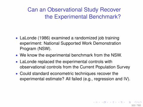
Can an Observational Study Recoverthe Experimental Benchmark?
• LaLonde (1986) examined a randomized job trainingexperiment: National Supported Work DemonstrationProgram (NSW).
• We know the experimental benchmark from the NSW.• LaLonde replaced the experimental controls with
observational controls from the Current Population Survey• Could standard econometric techniques recover the
experimental estimate? All failed (e.g., regression and IV).
322 / 765
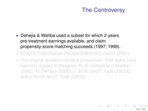
The Controversy
• Dehejia & Wahba used a subset for which 2-yearspre-treatment earnings available, and claimpropensity-score matching succeeds (1997; 1999).
• Smith & Todd dispute Dehejia & Wahba’s claims (2001).• The original question remains unresolved. Both sides have
basically agreed to disagree: R. H. Dehejia and Wahba(2002), R. Dehejia (2005), J. Smith and P. Todd (2005a),and J. Smith and P. Todd (2005b).
323 / 765
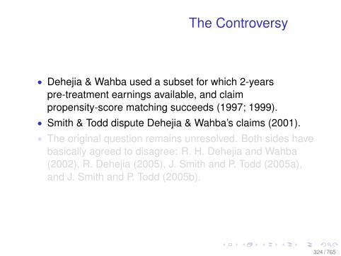
The Controversy
• Dehejia & Wahba used a subset for which 2-yearspre-treatment earnings available, and claimpropensity-score matching succeeds (1997; 1999).
• Smith & Todd dispute Dehejia & Wahba’s claims (2001).• The original question remains unresolved. Both sides have
basically agreed to disagree: R. H. Dehejia and Wahba(2002), R. Dehejia (2005), J. Smith and P. Todd (2005a),and J. Smith and P. Todd (2005b).
324 / 765
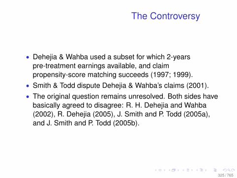
The Controversy
• Dehejia & Wahba used a subset for which 2-yearspre-treatment earnings available, and claimpropensity-score matching succeeds (1997; 1999).
• Smith & Todd dispute Dehejia & Wahba’s claims (2001).• The original question remains unresolved. Both sides have
basically agreed to disagree: R. H. Dehejia and Wahba(2002), R. Dehejia (2005), J. Smith and P. Todd (2005a),and J. Smith and P. Todd (2005b).
325 / 765
Genetic Matching (GenMatch)
Genetic matching is a new general method for performingmultivariate matching. GenMatch:• maximizes the balance of observed potential confounders
across matched treated and control units• uses an evolutionary search algorithm to determine the
weight each covariate is given• a genetic algorithm is used (Mebane and Sekhon, 2011)
326 / 765
Genetic Matching (GenMatch)
Genetic matching is a new general method for performingmultivariate matching. GenMatch:• maximizes the balance of observed potential confounders
across matched treated and control units• uses an evolutionary search algorithm to determine the
weight each covariate is given• a genetic algorithm is used (Mebane and Sekhon, 2011)
327 / 765

0.00 0.05 0.10 0.15 0.20 0.25
500
1000
1500
2000
2500
Dehejia Wahba Sample
Lowest p−value (KS & paired t−tests)
Est
imat
ed A
vera
ge T
reat
men
tt E
ffect
for
Tre
ated
($)
Experimental benchmark estimate ($1794)
328 / 765
GenMatch
• Debate arises because existing matching methods fail toobtain reliable levels of balance in this dataset.
• GenMatch is able to reliably estimate the causal effectswhen other methods fail because it achieves substantiallybetter balance.
• GenMatch in an hour produces vastly better balance thanhuman researchers working away for ten years.
329 / 765
GenMatch
• No information about any outcome is used• The method is nonparametric and does not depend on a
propensity score (pscore can be included)• Genetic matching can reduce the bias in X covariates in
cases where conventional methods of matching increasebias. Who general is this?
• If selection on observables holds, but EPBR does not, haslower bias and MSE in the estimand in the usualsimulations (will generally depend on loss function)
330 / 765
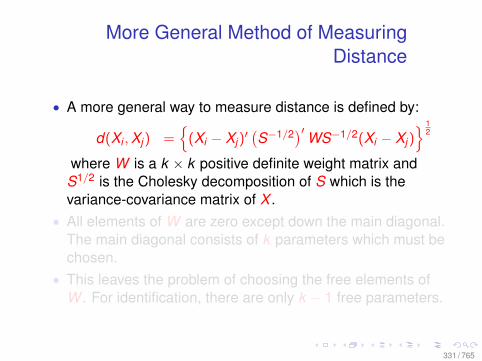
More General Method of MeasuringDistance
• A more general way to measure distance is defined by:
d(Xi ,Xj) =
(Xi − Xj)′ (S−1/2)′WS−1/2(Xi − Xj)
12
where W is a k × k positive definite weight matrix andS1/2 is the Cholesky decomposition of S which is thevariance-covariance matrix of X .
• All elements of W are zero except down the main diagonal.The main diagonal consists of k parameters which must bechosen.
• This leaves the problem of choosing the free elements ofW . For identification, there are only k − 1 free parameters.
331 / 765
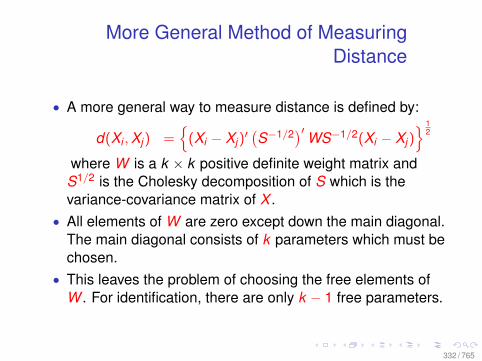
More General Method of MeasuringDistance
• A more general way to measure distance is defined by:
d(Xi ,Xj) =
(Xi − Xj)′ (S−1/2)′WS−1/2(Xi − Xj)
12
where W is a k × k positive definite weight matrix andS1/2 is the Cholesky decomposition of S which is thevariance-covariance matrix of X .
• All elements of W are zero except down the main diagonal.The main diagonal consists of k parameters which must bechosen.
• This leaves the problem of choosing the free elements ofW . For identification, there are only k − 1 free parameters.
332 / 765
Parameterization
• GenMatch uses the propensity score if it is known or if itcan be estimated.
• The propensity score is estimated and its linear predictor,µ, is matched upon along with the covariates X once theyhave been adjusted so as to be uncorrelated with the linearpredictor.
• Combining is good because:• Propensity score matching is good at minimizing the
discrepancy along the propensity score• Mahalanobis distance is good at minimizing the distance
between individual coordinates of X (orthogonal to thepropensity score) (P. R. Rosenbaum and Rubin, 1985).
333 / 765
Parameterization
• GenMatch uses the propensity score if it is known or if itcan be estimated.
• The propensity score is estimated and its linear predictor,µ, is matched upon along with the covariates X once theyhave been adjusted so as to be uncorrelated with the linearpredictor.
• Combining is good because:• Propensity score matching is good at minimizing the
discrepancy along the propensity score• Mahalanobis distance is good at minimizing the distance
between individual coordinates of X (orthogonal to thepropensity score) (P. R. Rosenbaum and Rubin, 1985).
334 / 765
Parameterization
• GenMatch uses the propensity score if it is known or if itcan be estimated.
• The propensity score is estimated and its linear predictor,µ, is matched upon along with the covariates X once theyhave been adjusted so as to be uncorrelated with the linearpredictor.
• Combining is good because:• Propensity score matching is good at minimizing the
discrepancy along the propensity score• Mahalanobis distance is good at minimizing the distance
between individual coordinates of X (orthogonal to thepropensity score) (P. R. Rosenbaum and Rubin, 1985).
335 / 765
Optimization
• Many loss functions are possible. Such as:• minimize the largest discrepancy• minimize the mean or median discrepancy• minimize some other quantile• restrict the above to only uniformly improving moves
• Our recommended algorithm attempts to minimize thelargest discrepancy at every step (minimizing the infinitynorm).
• For a given set of matches resulting from a given W , theloss is defined as the minimum p-value observed across aseries of balance tests.
336 / 765
Optimization
• Many loss functions are possible. Such as:• minimize the largest discrepancy• minimize the mean or median discrepancy• minimize some other quantile• restrict the above to only uniformly improving moves
• Our recommended algorithm attempts to minimize thelargest discrepancy at every step (minimizing the infinitynorm).
• For a given set of matches resulting from a given W , theloss is defined as the minimum p-value observed across aseries of balance tests.
337 / 765
Optimization
• Many loss functions are possible. Such as:• minimize the largest discrepancy• minimize the mean or median discrepancy• minimize some other quantile• restrict the above to only uniformly improving moves
• Our recommended algorithm attempts to minimize thelargest discrepancy at every step (minimizing the infinitynorm).
• For a given set of matches resulting from a given W , theloss is defined as the minimum p-value observed across aseries of balance tests.
338 / 765
Optimization
• Many loss functions are possible. Such as:• minimize the largest discrepancy• minimize the mean or median discrepancy• minimize some other quantile• restrict the above to only uniformly improving moves
• Our recommended algorithm attempts to minimize thelargest discrepancy at every step (minimizing the infinitynorm).
• For a given set of matches resulting from a given W , theloss is defined as the minimum p-value observed across aseries of balance tests.
339 / 765
Optimization
• Many loss functions are possible. Such as:• minimize the largest discrepancy• minimize the mean or median discrepancy• minimize some other quantile• restrict the above to only uniformly improving moves
• Our recommended algorithm attempts to minimize thelargest discrepancy at every step (minimizing the infinitynorm).
• For a given set of matches resulting from a given W , theloss is defined as the minimum p-value observed across aseries of balance tests.
340 / 765
Optimization
• Many loss functions are possible. Such as:• minimize the largest discrepancy• minimize the mean or median discrepancy• minimize some other quantile• restrict the above to only uniformly improving moves
• Our recommended algorithm attempts to minimize thelargest discrepancy at every step (minimizing the infinitynorm).
• For a given set of matches resulting from a given W , theloss is defined as the minimum p-value observed across aseries of balance tests.
341 / 765
Measuring Balance
• There are many different ways of testing for balance andwe cannot summarize the vast literature here.
• The choice of balance will be domain specific. E.g., userandomization inference if you can as Bowers and Hansen(2006) do.
• But the tests should be powerful and there should be manyoff them because different tests are sensitive to differentdepartures from balance.
• It is important the maximum discrepancy be small.p-values conventionally understood to signal balance (e.g.,0.10) are often too low to produce reliable estimates.
342 / 765
Measuring Balance
• There are many different ways of testing for balance andwe cannot summarize the vast literature here.
• The choice of balance will be domain specific. E.g., userandomization inference if you can as Bowers and Hansen(2006) do.
• But the tests should be powerful and there should be manyoff them because different tests are sensitive to differentdepartures from balance.
• It is important the maximum discrepancy be small.p-values conventionally understood to signal balance (e.g.,0.10) are often too low to produce reliable estimates.
343 / 765
Measuring Balance
• There are many different ways of testing for balance andwe cannot summarize the vast literature here.
• The choice of balance will be domain specific. E.g., userandomization inference if you can as Bowers and Hansen(2006) do.
• But the tests should be powerful and there should be manyoff them because different tests are sensitive to differentdepartures from balance.
• It is important the maximum discrepancy be small.p-values conventionally understood to signal balance (e.g.,0.10) are often too low to produce reliable estimates.
344 / 765
Measuring Balance
• There are many different ways of testing for balance andwe cannot summarize the vast literature here.
• The choice of balance will be domain specific. E.g., userandomization inference if you can as Bowers and Hansen(2006) do.
• But the tests should be powerful and there should be manyoff them because different tests are sensitive to differentdepartures from balance.
• It is important the maximum discrepancy be small.p-values conventionally understood to signal balance (e.g.,0.10) are often too low to produce reliable estimates.
345 / 765
Balance Tests
• the p-values from these balance tests cannot beinterpreted as true probabilities because of standardpre-test problems, but they remain useful measures ofbalance
• By default, tests are conducted for all univariate baselinecovariates, as well as their first-order interactions andquadratic terms.
• The analyst may add tests of any function of X desired,including additional nonlinear functions and higher orderinteractions.
• The tests conducted are t-tests for the difference of meansand nonparametric bootstrap Kolmogorov-Smirnovdistributional tests.
346 / 765
Balance Tests
• the p-values from these balance tests cannot beinterpreted as true probabilities because of standardpre-test problems, but they remain useful measures ofbalance
• By default, tests are conducted for all univariate baselinecovariates, as well as their first-order interactions andquadratic terms.
• The analyst may add tests of any function of X desired,including additional nonlinear functions and higher orderinteractions.
• The tests conducted are t-tests for the difference of meansand nonparametric bootstrap Kolmogorov-Smirnovdistributional tests.
347 / 765
Balance Tests
• the p-values from these balance tests cannot beinterpreted as true probabilities because of standardpre-test problems, but they remain useful measures ofbalance
• By default, tests are conducted for all univariate baselinecovariates, as well as their first-order interactions andquadratic terms.
• The analyst may add tests of any function of X desired,including additional nonlinear functions and higher orderinteractions.
• The tests conducted are t-tests for the difference of meansand nonparametric bootstrap Kolmogorov-Smirnovdistributional tests.
348 / 765
Balance Tests
• the p-values from these balance tests cannot beinterpreted as true probabilities because of standardpre-test problems, but they remain useful measures ofbalance
• By default, tests are conducted for all univariate baselinecovariates, as well as their first-order interactions andquadratic terms.
• The analyst may add tests of any function of X desired,including additional nonlinear functions and higher orderinteractions.
• The tests conducted are t-tests for the difference of meansand nonparametric bootstrap Kolmogorov-Smirnovdistributional tests.
349 / 765
Genetic Optimization
• The optimization problem described above is difficult andirregular, and we utilize an evolutionary algorithm calledGENOUD (Mebane and Sekhon, 2011)
• Random search also works better than the usual matchingmethods, but is less efficient than GENOUD.
350 / 765
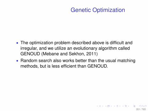
Genetic Optimization
• The optimization problem described above is difficult andirregular, and we utilize an evolutionary algorithm calledGENOUD (Mebane and Sekhon, 2011)
• Random search also works better than the usual matchingmethods, but is less efficient than GENOUD.
351 / 765
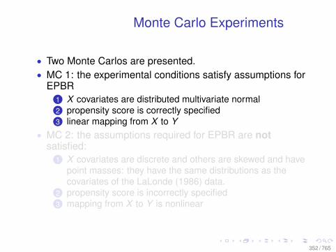
Monte Carlo Experiments
• Two Monte Carlos are presented.• MC 1: the experimental conditions satisfy assumptions for
EPBR1 X covariates are distributed multivariate normal2 propensity score is correctly specified3 linear mapping from X to Y
• MC 2: the assumptions required for EPBR are notsatisfied:
1 X covariates are discrete and others are skewed and havepoint masses: they have the same distributions as thecovariates of the LaLonde (1986) data.
2 propensity score is incorrectly specified3 mapping from X to Y is nonlinear
352 / 765
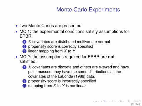
Monte Carlo Experiments
• Two Monte Carlos are presented.• MC 1: the experimental conditions satisfy assumptions for
EPBR1 X covariates are distributed multivariate normal2 propensity score is correctly specified3 linear mapping from X to Y
• MC 2: the assumptions required for EPBR are notsatisfied:
1 X covariates are discrete and others are skewed and havepoint masses: they have the same distributions as thecovariates of the LaLonde (1986) data.
2 propensity score is incorrectly specified3 mapping from X to Y is nonlinear
353 / 765
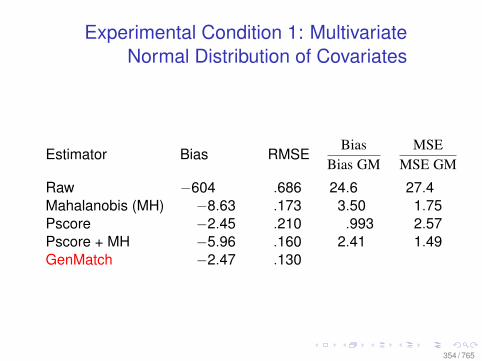
Experimental Condition 1: MultivariateNormal Distribution of Covariates
Estimator Bias RMSEBias
Bias GMMSE
MSE GM
Raw −604 .686 24.6 27.4Mahalanobis (MH) −8.63 .173 3.50 1.75Pscore −2.45 .210 .993 2.57Pscore + MH −5.96 .160 2.41 1.49GenMatch −2.47 .130
354 / 765
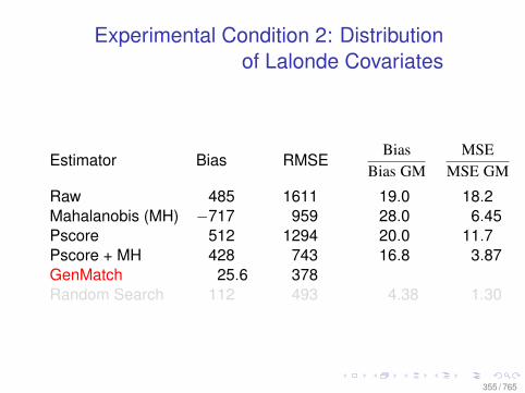
Experimental Condition 2: Distributionof Lalonde Covariates
Estimator Bias RMSEBias
Bias GMMSE
MSE GM
Raw 485 1611 19.0 18.2Mahalanobis (MH) −717 959 28.0 6.45Pscore 512 1294 20.0 11.7Pscore + MH 428 743 16.8 3.87GenMatch 25.6 378Random Search 112 493 4.38 1.30
355 / 765
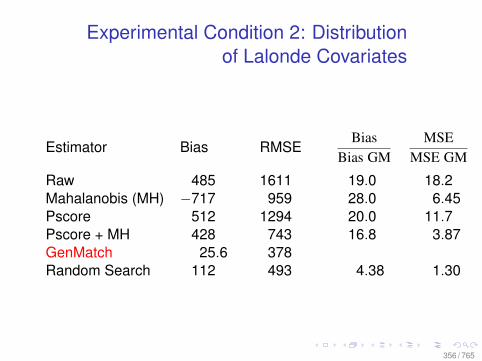
Experimental Condition 2: Distributionof Lalonde Covariates
Estimator Bias RMSEBias
Bias GMMSE
MSE GM
Raw 485 1611 19.0 18.2Mahalanobis (MH) −717 959 28.0 6.45Pscore 512 1294 20.0 11.7Pscore + MH 428 743 16.8 3.87GenMatch 25.6 378Random Search 112 493 4.38 1.30
356 / 765
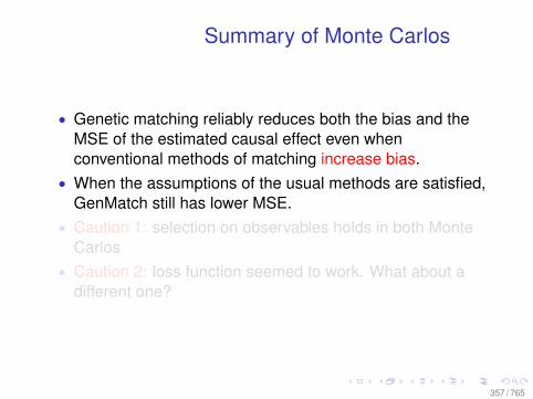
Summary of Monte Carlos
• Genetic matching reliably reduces both the bias and theMSE of the estimated causal effect even whenconventional methods of matching increase bias.
• When the assumptions of the usual methods are satisfied,GenMatch still has lower MSE.
• Caution 1: selection on observables holds in both MonteCarlos
• Caution 2: loss function seemed to work. What about adifferent one?
357 / 765

Summary of Monte Carlos
• Genetic matching reliably reduces both the bias and theMSE of the estimated causal effect even whenconventional methods of matching increase bias.
• When the assumptions of the usual methods are satisfied,GenMatch still has lower MSE.
• Caution 1: selection on observables holds in both MonteCarlos
• Caution 2: loss function seemed to work. What about adifferent one?
358 / 765
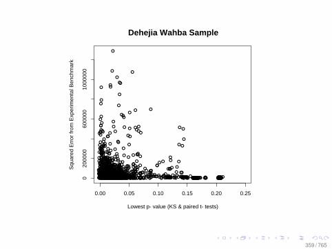
0.00 0.05 0.10 0.15 0.20 0.25
020
0000
6000
0010
0000
0
Dehejia Wahba Sample
Lowest p−value (KS & paired t−tests)
Squ
ared
Err
or fr
om E
xper
imen
tal B
ench
mar
k
359 / 765
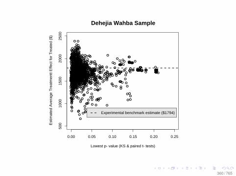
0.00 0.05 0.10 0.15 0.20 0.25
500
1000
1500
2000
2500
Dehejia Wahba Sample
Lowest p−value (KS & paired t−tests)
Est
imat
ed A
vera
ge T
reat
men
tt E
ffect
for
Tre
ated
($)
Experimental benchmark estimate ($1794)
360 / 765
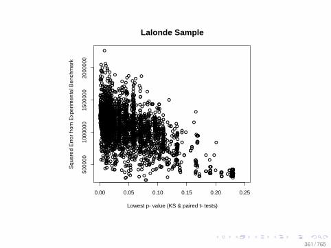
0.00 0.05 0.10 0.15 0.20 0.25
5000
0010
0000
015
0000
020
0000
0
Lalonde Sample
Lowest p−value (KS & paired t−tests)
Squ
ared
Err
or fr
om E
xper
imen
tal B
ench
mar
k
361 / 765
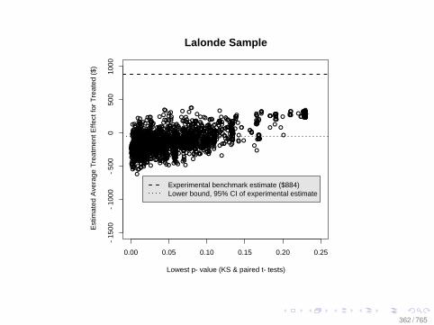
0.00 0.05 0.10 0.15 0.20 0.25
−15
00−
1000
−50
00
500
1000
Lalonde Sample
Lowest p−value (KS & paired t−tests)
Est
imat
ed A
vera
ge T
reat
men
t Effe
ct fo
r T
reat
ed (
$)
Experimental benchmark estimate ($884)Lower bound, 95% CI of experimental estimate
362 / 765
Mahalanobis Distance
• Distributions of Xs are not ellipsoidal, so there’s no reasonto think MD will work• Dehejia Wahba sample: balance is poor, but estimates are
right on target!• LaLonde sample: balance exceeds conventional standards,
but estimates are off the mark
• Lesson: Don’t count on getting lucky. Instead, achieve bestpossible balance, and look at outcomes only once, afterbalance is attained.
363 / 765
Mahalanobis Distance
• Distributions of Xs are not ellipsoidal, so there’s no reasonto think MD will work• Dehejia Wahba sample: balance is poor, but estimates are
right on target!• LaLonde sample: balance exceeds conventional standards,
but estimates are off the mark
• Lesson: Don’t count on getting lucky. Instead, achieve bestpossible balance, and look at outcomes only once, afterbalance is attained.
364 / 765
Mahalanobis Distance
• Distributions of Xs are not ellipsoidal, so there’s no reasonto think MD will work• Dehejia Wahba sample: balance is poor, but estimates are
right on target!• LaLonde sample: balance exceeds conventional standards,
but estimates are off the mark
• Lesson: Don’t count on getting lucky. Instead, achieve bestpossible balance, and look at outcomes only once, afterbalance is attained.
365 / 765
GenMatch Summary
• GenMatch in an hour produces vastly better balance thanhuman researchers working away for ten years.
• Machine learning can come to the rescue• But without the RCT, we would have a debate of how much
to adjust• Caution is warranted• No amount of statistical modeling or algorithmic wizardry
can resolve these questions
366 / 765
GenMatch Summary
• GenMatch in an hour produces vastly better balance thanhuman researchers working away for ten years.
• Machine learning can come to the rescue• But without the RCT, we would have a debate of how much
to adjust• Caution is warranted• No amount of statistical modeling or algorithmic wizardry
can resolve these questions
367 / 765
Opiates for the Matches
• Rubin: design trumps analysisbut design cannot be mass produced
• Selection on observables assumed too readily:• no design• difficult questions about inference ignored• balance checks are rudimentary• no placebo tests
• ties to Neyman-Rubin model weakening• how well does it work in practice?• statistical theory is of little guidance
368 / 765
Opiates for the Matches
• Rubin: design trumps analysisbut design cannot be mass produced
• Selection on observables assumed too readily:• no design• difficult questions about inference ignored• balance checks are rudimentary• no placebo tests
• ties to Neyman-Rubin model weakening• how well does it work in practice?• statistical theory is of little guidance
369 / 765
Opiates for the Matches
• Rubin: design trumps analysisbut design cannot be mass produced
• Selection on observables assumed too readily:• no design• difficult questions about inference ignored• balance checks are rudimentary• no placebo tests
• ties to Neyman-Rubin model weakening• how well does it work in practice?• statistical theory is of little guidance
370 / 765
Public Health and Medical Literature
• Use of matching has a longer history• Many more experiments so a hope of calibration• The interventions are actually done: another source of
calibration• But resistance to comparing experiments with
observational studies:• external validity• heterogeneous causal effect: casemix• private data (e.g., Hormone Replacement Therapy)
371 / 765

Public Health and Medical Literature
• Use of matching has a longer history• Many more experiments so a hope of calibration• The interventions are actually done: another source of
calibration• But resistance to comparing experiments with
observational studies:• external validity• heterogeneous causal effect: casemix• private data (e.g., Hormone Replacement Therapy)
372 / 765
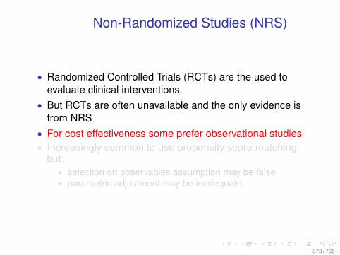
Non-Randomized Studies (NRS)
• Randomized Controlled Trials (RCTs) are the used toevaluate clinical interventions.
• But RCTs are often unavailable and the only evidence isfrom NRS
• For cost effectiveness some prefer observational studies• Increasingly common to use propensity score matching,
but:• selection on observables assumption may be false• parametric adjustment may be inadequate
373 / 765
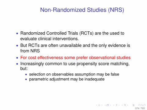
Non-Randomized Studies (NRS)
• Randomized Controlled Trials (RCTs) are the used toevaluate clinical interventions.
• But RCTs are often unavailable and the only evidence isfrom NRS
• For cost effectiveness some prefer observational studies• Increasingly common to use propensity score matching,
but:• selection on observables assumption may be false• parametric adjustment may be inadequate
374 / 765

Summary
• Example: evaluation of Pulmonary Artery Catheterization(PAC) versus no-PAC. NRS found that PAC significantlyincreases mortality while the RCT found no difference inmortality. Sekhon and Grieve 2008
• Genetic Matching gives similar results to the RCT butusing the NRS
• People failed to check balance after spending million ofdollars collecting the data
• They didn’t even plot the data
375 / 765

Pulmonary Artery Catheterization(PAC)
• PAC is an invasive cardiac monitoring device for critical illpatients (ICU)—e.g., myocardial infarction (ischaemicheart disease)
• Widely used for the past 30 years: spend $2 billion in U.S.per year
• RCT find no effect; seven NRS find that PAC increasesmortality (e.g., Connors et al. JAMA 1996)
• RCT: causal effect really is zero• Why do seven NRS disagree with RCTs?
376 / 765

Pulmonary Artery Catheterization(PAC)
• PAC is an invasive cardiac monitoring device for critical illpatients (ICU)—e.g., myocardial infarction (ischaemicheart disease)
• Widely used for the past 30 years: spend $2 billion in U.S.per year
• RCT find no effect; seven NRS find that PAC increasesmortality (e.g., Connors et al. JAMA 1996)
• RCT: causal effect really is zero• Why do seven NRS disagree with RCTs?
377 / 765

PAC
• NRS all ICU admissions to 57 UK ICUs 2003-4• 1052 cases with PAC; 32,499 controls (from a database of
N≈2M)• Propensity score model: Age, reasons for admission,
organ failure, probability of death, LOS, teaching hospital,size of unit
• logistic regression, predict p (PAC)• match on propensity score• GenMatch: p score and the same underlying covariates
multivariate matching algorithm, to max balance
378 / 765
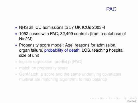
PAC
• NRS all ICU admissions to 57 UK ICUs 2003-4• 1052 cases with PAC; 32,499 controls (from a database of
N≈2M)• Propensity score model: Age, reasons for admission,
organ failure, probability of death, LOS, teaching hospital,size of unit
• logistic regression, predict p (PAC)• match on propensity score• GenMatch: p score and the same underlying covariates
multivariate matching algorithm, to max balance
379 / 765
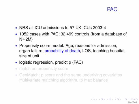
PAC
• NRS all ICU admissions to 57 UK ICUs 2003-4• 1052 cases with PAC; 32,499 controls (from a database of
N≈2M)• Propensity score model: Age, reasons for admission,
organ failure, probability of death, LOS, teaching hospital,size of unit
• logistic regression, predict p (PAC)• match on propensity score• GenMatch: p score and the same underlying covariates
multivariate matching algorithm, to max balance
380 / 765
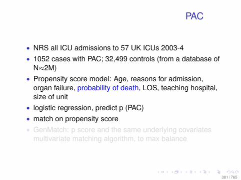
PAC
• NRS all ICU admissions to 57 UK ICUs 2003-4• 1052 cases with PAC; 32,499 controls (from a database of
N≈2M)• Propensity score model: Age, reasons for admission,
organ failure, probability of death, LOS, teaching hospital,size of unit
• logistic regression, predict p (PAC)• match on propensity score• GenMatch: p score and the same underlying covariates
multivariate matching algorithm, to max balance
381 / 765
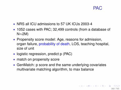
PAC
• NRS all ICU admissions to 57 UK ICUs 2003-4• 1052 cases with PAC; 32,499 controls (from a database of
N≈2M)• Propensity score model: Age, reasons for admission,
organ failure, probability of death, LOS, teaching hospital,size of unit
• logistic regression, predict p (PAC)• match on propensity score• GenMatch: p score and the same underlying covariates
multivariate matching algorithm, to max balance
382 / 765
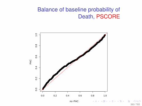
Balance of baseline probability ofDeath, PSCORE
0.0 0.2 0.4 0.6 0.8 1.0
0.0
0.2
0.4
0.6
0.8
1.0
no−PAC
PA
C
383 / 765
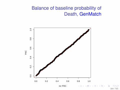
Balance of baseline probability ofDeath, GenMatch
0.0 0.2 0.4 0.6 0.8 1.0
0.0
0.2
0.4
0.6
0.8
1.0
no−PAC
PA
C
384 / 765
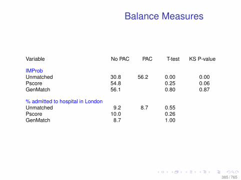
Balance Measures
Variable No PAC PAC T-test KS P-value
IMProbUnmatched 30.8 56.2 0.00 0.00Pscore 54.8 0.25 0.06GenMatch 56.1 0.80 0.87
% admitted to hospital in LondonUnmatched 9.2 8.7 0.55Pscore 10.0 0.26GenMatch 8.7 1.00
385 / 765

Balance Measures
Variable No PAC PAC KS P-value
AgeUnmatched 30.8 56.2 0.00Pscore 54.8 0.06GenMatch 56.1 0.87
% admitted for emergency surgeryUnmatched 20.2 23.1 0.03Pscore 21.3 0.32GenMatch 23.7 0.66
% admitted to teaching hospitalUnmatched 37.7 42.6 0.00Pscore 44.5 0.38GenMatch 42.6 1.00
386 / 765
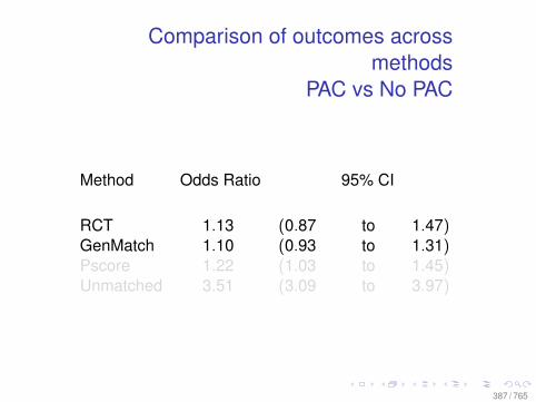
Comparison of outcomes acrossmethods
PAC vs No PAC
Method Odds Ratio 95% CI
RCT 1.13 (0.87 to 1.47)GenMatch 1.10 (0.93 to 1.31)Pscore 1.22 (1.03 to 1.45)Unmatched 3.51 (3.09 to 3.97)
387 / 765
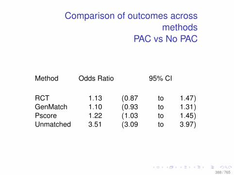
Comparison of outcomes acrossmethods
PAC vs No PAC
Method Odds Ratio 95% CI
RCT 1.13 (0.87 to 1.47)GenMatch 1.10 (0.93 to 1.31)Pscore 1.22 (1.03 to 1.45)Unmatched 3.51 (3.09 to 3.97)
388 / 765
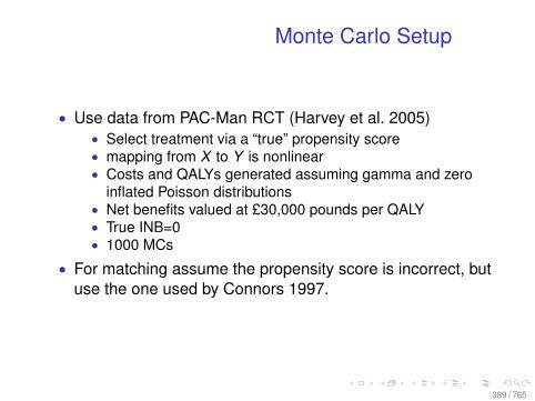
Monte Carlo Setup
• Use data from PAC-Man RCT (Harvey et al. 2005)• Select treatment via a “true” propensity score• mapping from X to Y is nonlinear• Costs and QALYs generated assuming gamma and zero
inflated Poisson distributions• Net benefits valued at £30,000 pounds per QALY• True INB=0• 1000 MCs
• For matching assume the propensity score is incorrect, butuse the one used by Connors 1997.
389 / 765
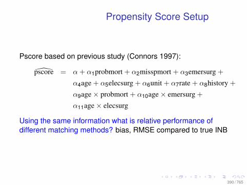
Propensity Score Setup
Pscore based on previous study (Connors 1997):
pscore = α + α1probmort + α2misspmort + α3emersurg +
α4age + α5elecsurg + α6unit + α7rate + α8history +
α9age× probmort + α10age× emersurg +
α11age× elecsurg
Using the same information what is relative performance ofdifferent matching methods? bias, RMSE compared to true INB
390 / 765
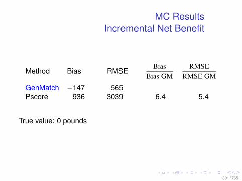
MC ResultsIncremental Net Benefit
Method Bias RMSEBias
Bias GMRMSE
RMSE GM
GenMatch −147 565Pscore 936 3039 6.4 5.4
True value: 0 pounds
391 / 765

Conclusion
• NICE (National Institute of Clinical Medicine) is coming tothe U.S. in some form
• Cost effectiveness uses NRS more than FDA typeregulators
• The biases are profound, even when selection onobservables holds
• Variance estimates profoundly underestimate the trueuncertainty
• Most extant objections are moral: I have a scientificconcern
• What does this say about our field?
392 / 765
Conclusion
• NICE (National Institute of Clinical Medicine) is coming tothe U.S. in some form
• Cost effectiveness uses NRS more than FDA typeregulators
• The biases are profound, even when selection onobservables holds
• Variance estimates profoundly underestimate the trueuncertainty
• Most extant objections are moral: I have a scientificconcern
• What does this say about our field?
393 / 765
Conclusion
• NICE (National Institute of Clinical Medicine) is coming tothe U.S. in some form
• Cost effectiveness uses NRS more than FDA typeregulators
• The biases are profound, even when selection onobservables holds
• Variance estimates profoundly underestimate the trueuncertainty
• Most extant objections are moral: I have a scientificconcern
• What does this say about our field?
394 / 765
Conclusion
• Machine learning can help solve the easy problem ofbalance
• GenMatch achieves excellent covariate balance• It gives similar results to the RCT• But without the RCT, we would have a debate of how much
to adjust• Caution is warranted• Talking NICE into releasing observational data before
parallel RCT results
395 / 765
Conclusion
• Machine learning can help solve the easy problem ofbalance
• GenMatch achieves excellent covariate balance• It gives similar results to the RCT• But without the RCT, we would have a debate of how much
to adjust• Caution is warranted• Talking NICE into releasing observational data before
parallel RCT results
396 / 765
The Problem
• When overcoming identification problems, we often turn torandomized controlled trials (RCTs)
• Often, though, RCTs are not a feasible, so we turn toobservational studies, or non-random studies (NRSs)
• The problem, then, is how to combine this information inorder to provide evidence for treatment effects in the fullpopulation of interest.• RCTs raise issues of Randomization Bias (Heckman and
J. A. Smith, 1995): poor external validity• NRSs raise issues of Selection Bias, or non random
assignment to treatment: poor internal validity
397 / 765
The Opportunity
• Explosion of data sources: administrative, electronicmedical records (EMR), online behavior
• Population data is becoming more common and moreprecise
• How can it be used?
• Policy makers/firms:“let’s just use the big data to make causal inference”
• Tension between identification vs. machinelearning/prediction
398 / 765
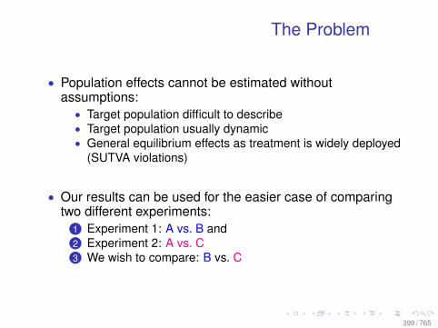
The Problem
• Population effects cannot be estimated withoutassumptions:• Target population difficult to describe• Target population usually dynamic• General equilibrium effects as treatment is widely deployed
(SUTVA violations)
• Our results can be used for the easier case of comparingtwo different experiments:
1 Experiment 1: A vs. B and2 Experiment 2: A vs. C3 We wish to compare: B vs. C
399 / 765

Example
• A growing interest in the cost of health care• Interest in system-wide issues—e.g., Dartmouth Atlas of
Health Care• Comparing the cost of UCLA versus Mayo Clinic is a
causal question• Comparing the cost and health outcomes in the USA
versus UK is also a causal question, but a less clear one• We examine a simple case: conduct a cost effectiveness
analysis (CEA) for one medical procedure
400 / 765

Example
• A growing interest in the cost of health care• Interest in system-wide issues—e.g., Dartmouth Atlas of
Health Care• Comparing the cost of UCLA versus Mayo Clinic is a
causal question• Comparing the cost and health outcomes in the USA
versus UK is also a causal question, but a less clear one• We examine a simple case: conduct a cost effectiveness
analysis (CEA) for one medical procedure
401 / 765
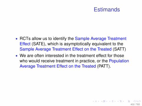
Estimands
• RCTs allow us to identify the Sample Average TreatmentEffect (SATE), which is asymptotically equivalent to theSample Average Treatment Effect on the Treated (SATT)
• We are often interested in the treatment effect for thosewho would receive treatment in practice, or the PopulationAverage Treatment Effect on the Treated (PATT).
402 / 765
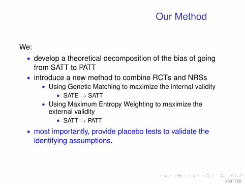
Our Method
We:• develop a theoretical decomposition of the bias of going
from SATT to PATT• introduce a new method to combine RCTs and NRSs
• Using Genetic Matching to maximize the internal validity• SATE→ SATT
• Using Maximum Entropy Weighting to maximize theexternal validity• SATT→ PATT
• most importantly, provide placebo tests to validate theidentifying assumptions.
403 / 765

Pulmonary Artery Catheterization(PAC)
• PAC is an invasive cardiac monitoring device for critical illpatients (ICU)—e.g., myocardial infarction (ischaemicheart disease)
• Widely used for the past 30 years: spend $2 billion in U.S.per year
• RCT find no effect; seven NRS find that PAC increasesmortality (e.g., Connors et al. JAMA 1996)
404 / 765

Pulmonary Artery Catheterization
• RCT: a publicly funded, pragmatic experiment done in 65UK ICUs in 2000-2004.• 1014 subjects, 506 who received PAC• No difference in hospital mortality (p = 0.39)
• NRS: all ICU admissions to 57 UK ICUs in 2003-2004• 1052 cases with PAC and 32,499 controls• One observational study was able to find no difference in
hospital mortality (p = 0.29)
• However, the populations between the two studies differ,and we are interested in identifying PATT.
405 / 765

Schematic of SATE to PATT
In the next figure: double arrows indicate exchangeability ofpotential outcomes and dashed arrows indicate adjustment ofthe covariate distribution
406 / 765
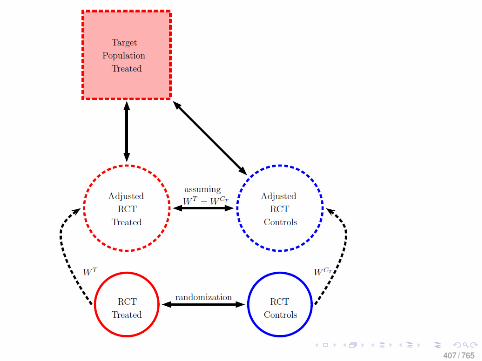
407 / 765
We can think of the bias in our estimate of the PATT as acombination of bias due to a possible lack of internal validity ofthe estimate of SATT and bias due to poor external validity ofthe estimate from the RCT.
B = BI + BE
We can decompose of these biases in more detail as anextension of the Heckman, Ichimura, et al. (1998)decomposition of bias.
408 / 765
Some Definitions
• Let X denote a set of conditioning covariates in the samplepopulation and W denote a set of conditioning covariatesin the target population
• Let Y1 and Y0 denote the potential outcomes for a subject i• Let T ∈ (0,1) be an indicator for whether or not subject i
was in the treatment or control group• Let I ∈ (0,1) be an indicator for whether or not subject i
was in the sample population
409 / 765

BI = ES11\SI1E(Y0|X ,T = 1, I = 1)
− ES10\SI1E(Y0|X ,T = 0, I = 1)
+ EdF (T =1)−dF (T =0),SI1E(Y0|X ,T = 0, I = 1)
+ EdF (T =1),SI1E(Y0|X ,T = 1, I = 1)− E(Y0|X ,T = 0, I = 1)
The internal validity problem is due to bias in the RCT estimateof SATT.
410 / 765
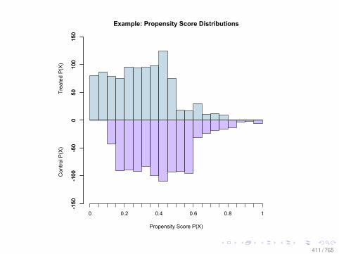
Example: Propensity Score Distributions
Propensity Score P(X)
-150
-100
-50
050
100
150
-150
-100
-50
050
100
150
0 0.2 0.4 0.6 0.8 1
Con
trol P
(X)
Trea
ted
P(X
)
411 / 765
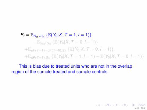
BI = ES11\SI1E(Y0|X ,T = 1, I = 1)
−ES10\SI1E(Y0|X ,T = 0, I = 1)
+EdF (T =1)−dF (T =0),SI1E(Y0|X ,T = 0, I = 1)
+EdF (T =1),SI1E(Y0|X ,T = 1, I = 1)− E(Y0|X ,T = 0, I = 1)
This is bias due to treated units who are not in the overlapregion of the sample treated and sample controls.
412 / 765
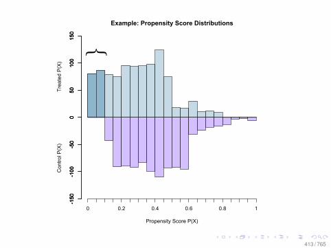
Example: Propensity Score Distributions
Propensity Score P(X)
-150
-100
-50
050
100
150
-150
-100
-50
050
100
150
-150
-100
-50
050
100
150
0 0.2 0.4 0.6 0.8 1
Con
trol P
(X)
Trea
ted
P(X
)
413 / 765
BI = ES11\SI1E(Y0|X ,T = 1, I = 1)
−ES10\SI1E(Y0|X ,T = 0, I = 1)
+EdF (T =1)−dF (T =0),SI1E(Y0|X ,T = 0, I = 1)
+EdF (T =1),SI1E(Y0|X ,T = 1, I = 1)− E(Y0|X ,T = 0, I = 1)
This is bias due to controls units who are not in the overlapregion of the sample treated and sample controls.
414 / 765
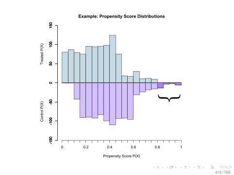
Example: Propensity Score Distributions
Propensity Score P(X)
-150
-100
-50
050
100
150
-150
-100
-50
050
100
150
-150
-100
-50
050
100
150
0 0.2 0.4 0.6 0.8 1
Con
trol P
(X)
Trea
ted
P(X
)
415 / 765
BI = ES11\SI1E(Y0|X ,T = 1, I = 1)
−ES10\SI1E(Y0|X ,T = 0, I = 1)
+EdF (T =1)−dF (T =0),SI1E(Y0|X ,T = 0, I = 1)
+EdF (T =1),SI1E(Y0|X ,T = 1, I = 1)− E(Y0|X ,T = 0, I = 1)
This is bias due to imbalance of the sample treated andsample control units in the overlap region.
416 / 765
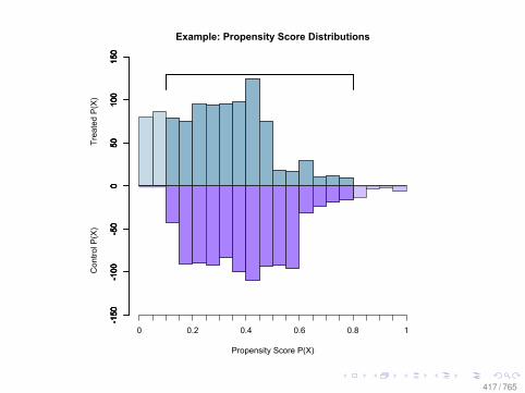
Example: Propensity Score Distributions
Propensity Score P(X)
-150
-100
-50
050
100
150
-150
-100
-50
050
100
150
-150
-100
-50
050
100
150
-150
-100
-50
050
100
150
0 0.2 0.4 0.6 0.8 1
Con
trol P
(X)
Trea
ted
P(X
)
417 / 765
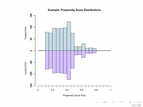
Example: Propensity Score Distributions
Propensity Score P(X)
-150
-100
-50
050
100
150
-150
-100
-50
050
100
150
0 0.2 0.4 0.6 0.8 1
Con
trol P
(X)
Trea
ted
P(X
)
418 / 765
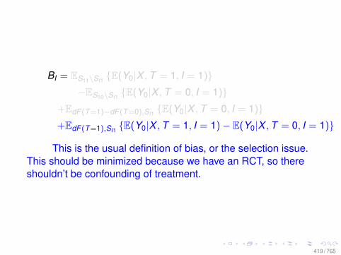
BI = ES11\SI1E(Y0|X ,T = 1, I = 1)
−ES10\SI1E(Y0|X ,T = 0, I = 1)
+EdF (T =1)−dF (T =0),SI1E(Y0|X ,T = 0, I = 1)
+EdF (T =1),SI1E(Y0|X ,T = 1, I = 1)− E(Y0|X ,T = 0, I = 1)
This is the usual definition of bias, or the selection issue.This should be minimized because we have an RCT, so thereshouldn’t be confounding of treatment.
419 / 765
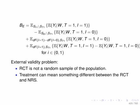
BE = ES11\ST1E(Yi |W ,T = 1, I = 1)
− ES01\ST1E(Yi |W ,T = 1, I = 0)
+ EdF (I=1)−dF (I=0),ST1E(Yi |W ,T = 1, I = 0)
+ EdF (I=1),ST1E(Yi |W ,T = 1, I = 1)− E(Yi |W ,T = 1, I = 0)
for i ∈ (0,1)
External validity problem:• RCT is not a random sample of the population.• Treatment can mean something different between the RCT
and NRS.
420 / 765
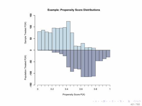
Example: Propensity Score Distributions
Propensity Score P(X)
-150
-100
-50
050
100
150
-150
-100
-50
050
100
150
0 0.2 0.4 0.6 0.8 1
Pop
ulat
ion
Trea
ted
P(W
)S
ampl
e Tr
eate
d P
(W)
421 / 765
BE = ES11\ST1E(Yi |W ,T = 1, I = 1)
−ES01\ST1E(Yi |W ,T = 1, I = 0)
+EdF (I=1)−dF (I=0),ST 1E(Yi |W ,T = 1, I = 0)
+EdF (I=1),ST1E(Yi |W ,T = 1, I = 1)− E(Yi |W ,T = 1, I = 0)
for i ∈ (0,1)
This is bias due to sample treated units who are not in theoverlap region of the sample treated and population treated.
422 / 765
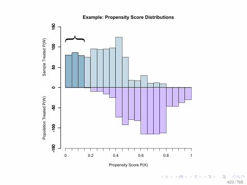
Example: Propensity Score Distributions
Propensity Score P(X)
-150
-100
-50
050
100
150
-150
-100
-50
050
100
150
-150
-100
-50
050
100
150
0 0.2 0.4 0.6 0.8 1
Pop
ulat
ion
Trea
ted
P(W
)S
ampl
e Tr
eate
d P
(W)
423 / 765
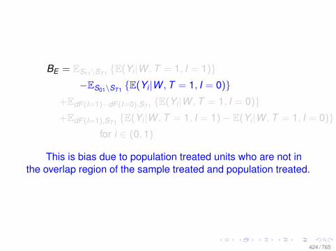
BE = ES11\ST1E(Yi |W ,T = 1, I = 1)
−ES01\ST1E(Yi |W ,T = 1, I = 0)
+EdF (I=1)−dF (I=0),ST 1E(Yi |W ,T = 1, I = 0)
+EdF (I=1),ST1E(Yi |W ,T = 1, I = 1)− E(Yi |W ,T = 1, I = 0)
for i ∈ (0,1)
This is bias due to population treated units who are not inthe overlap region of the sample treated and population treated.
424 / 765
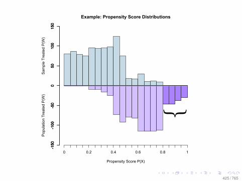
Example: Propensity Score Distributions
Propensity Score P(X)
-150
-100
-50
050
100
150
-150
-100
-50
050
100
150
-150
-100
-50
050
100
150
0 0.2 0.4 0.6 0.8 1
Pop
ulat
ion
Trea
ted
P(W
)S
ampl
e Tr
eate
d P
(W)
425 / 765
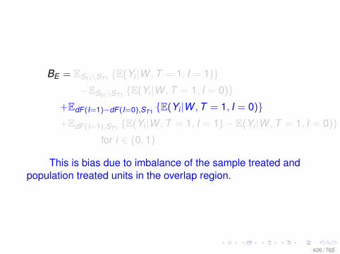
BE = ES11\ST1E(Yi |W ,T = 1, I = 1)
−ES01\ST1E(Yi |W ,T = 1, I = 0)
+EdF (I=1)−dF (I=0),ST 1E(Yi |W ,T = 1, I = 0)
+EdF (I=1),ST1E(Yi |W ,T = 1, I = 1)− E(Yi |W ,T = 1, I = 0)
for i ∈ (0,1)
This is bias due to imbalance of the sample treated andpopulation treated units in the overlap region.
426 / 765
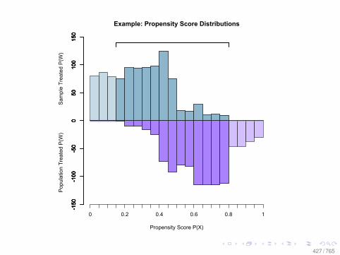
Example: Propensity Score Distributions
Propensity Score P(X)
-150
-100
-50
050
100
150
-150
-100
-50
050
100
150
-150
-100
-50
050
100
150
-150
-100
-50
050
100
150
0 0.2 0.4 0.6 0.8 1
Pop
ulat
ion
Trea
ted
P(W
)S
ampl
e Tr
eate
d P
(W)
427 / 765
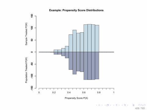
Example: Propensity Score Distributions
Propensity Score P(X)
-150
-100
-50
050
100
150
-150
-100
-50
050
100
150
0 0.2 0.4 0.6 0.8 1
Pop
ulat
ion
Trea
ted
P(W
)S
ampl
e Tr
eate
d P
(W)
428 / 765
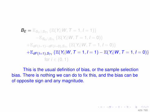
BE = ES11\ST1E(Yi |W ,T = 1, I = 1)
−ES01\ST1E(Yi |W ,T = 1, I = 0)
+EdF (I=1)−dF (I=0),ST 1E(Yi |W ,T = 1, I = 0)
+EdF (I=1),ST1E(Yi |W ,T = 1, I = 1)− E(Yi |W ,T = 1, I = 0)
for i ∈ (0,1)
This is the usual definition of bias, or the sample selectionbias. There is nothing we can do to fix this, and the bias can beof opposite sign and any magnitude.
429 / 765
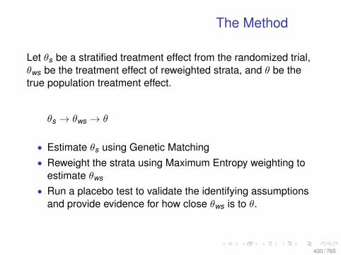
The Method
Let θs be a stratified treatment effect from the randomized trial,θws be the treatment effect of reweighted strata, and θ be thetrue population treatment effect.
θs → θws → θ
• Estimate θs using Genetic Matching• Reweight the strata using Maximum Entropy weighting to
estimate θws
• Run a placebo test to validate the identifying assumptionsand provide evidence for how close θws is to θ.
430 / 765
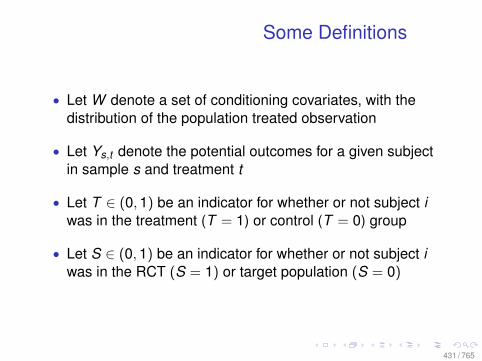
Some Definitions
• Let W denote a set of conditioning covariates, with thedistribution of the population treated observation
• Let Ys,t denote the potential outcomes for a given subjectin sample s and treatment t
• Let T ∈ (0,1) be an indicator for whether or not subject iwas in the treatment (T = 1) or control (T = 0) group
• Let S ∈ (0,1) be an indicator for whether or not subject iwas in the RCT (S = 1) or target population (S = 0)
431 / 765
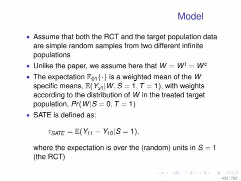
Model
• Assume that both the RCT and the target population dataare simple random samples from two different infinitepopulations
• Unlike the paper, we assume here that W = W t = W c
• The expectation E01· is a weighted mean of the Wspecific means, E(Ys1|W ,S = 1,T = 1), with weightsaccording to the distribution of W in the treated targetpopulation, Pr(W |S = 0,T = 1)
• SATE is defined as:
τSATE = E(Y11 − Y10|S = 1),
where the expectation is over the (random) units in S = 1(the RCT)
432 / 765
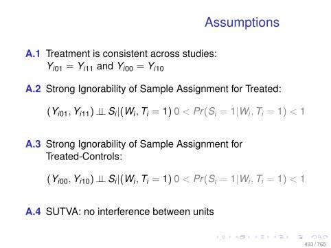
Assumptions
A.1 Treatment is consistent across studies:Yi01 = Yi11 and Yi00 = Yi10
A.2 Strong Ignorability of Sample Assignment for Treated:
(Yi01,Yi11)⊥⊥Si |(Wi ,Ti = 1) 0 < Pr(Si = 1|Wi ,Ti = 1) < 1
A.3 Strong Ignorability of Sample Assignment forTreated-Controls:
(Yi00,Yi10)⊥⊥Si |(Wi ,Ti = 1) 0 < Pr(Si = 1|Wi ,Ti = 1) < 1
A.4 SUTVA: no interference between units
433 / 765
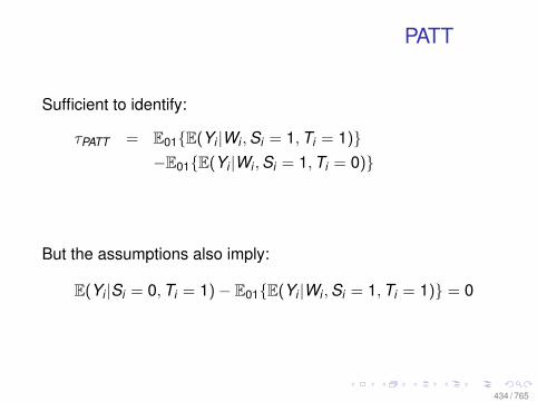
PATT
Sufficient to identify:
τPATT = E01E(Yi |Wi ,Si = 1,Ti = 1)−E01E(Yi |Wi ,Si = 1,Ti = 0)
But the assumptions also imply:
E(Yi |Si = 0,Ti = 1)− E01E(Yi |Wi ,Si = 1,Ti = 1) = 0
434 / 765
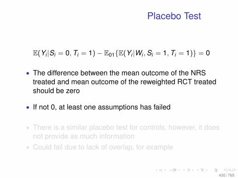
Placebo Test
E(Yi |Si = 0,Ti = 1)− E01E(Yi |Wi ,Si = 1,Ti = 1) = 0
• The difference between the mean outcome of the NRStreated and mean outcome of the reweighted RCT treatedshould be zero
• If not 0, at least one assumptions has failed
• There is a similar placebo test for controls, however, it doesnot provide as much information
• Could fail due to lack of overlap, for example
435 / 765
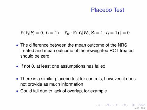
Placebo Test
E(Yi |Si = 0,Ti = 1)− E01E(Yi |Wi ,Si = 1,Ti = 1) = 0
• The difference between the mean outcome of the NRStreated and mean outcome of the reweighted RCT treatedshould be zero
• If not 0, at least one assumptions has failed
• There is a similar placebo test for controls, however, it doesnot provide as much information
• Could fail due to lack of overlap, for example
436 / 765
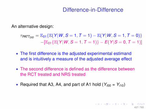
Difference-in-Difference
An alternative design:
τPATTDID = E01E(Y |W ,S = 1,T = 1)− E(Y |W ,S = 1,T = 0)−[E01E(Y |W ,S = 1,T = 1) − E(Y |S = 0,T = 1)]
• The first difference is the adjusted experimental estimandand is intuitively a measure of the adjusted average effect
• The second difference is defined as the difference betweenthe RCT treated and NRS treated
• Required that A3, A4, and part of A1 hold (Yi00 = Yi10)
437 / 765
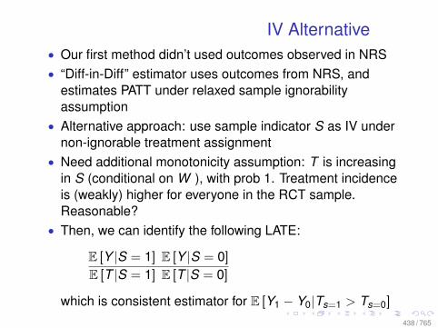
IV Alternative• Our first method didn’t used outcomes observed in NRS• “Diff-in-Diff” estimator uses outcomes from NRS, and
estimates PATT under relaxed sample ignorabilityassumption
• Alternative approach: use sample indicator S as IV undernon-ignorable treatment assignment
• Need additional monotonicity assumption: T is increasingin S (conditional on W ), with prob 1. Treatment incidenceis (weakly) higher for everyone in the RCT sample.Reasonable?
• Then, we can identify the following LATE:
E [Y |S = 1] E [Y |S = 0]
E [T |S = 1] E [T |S = 0]
which is consistent estimator for E [Y1 − Y0|Ts=1 > Ts=0]
438 / 765
Statistical Methods
GenMatch:• Matching method with automated balance optimization.
Maximum Entropy weighting:• Weighting method that assigns weights such that they
simultaneously meet a set of consistency constraints whilemaximizing Shannon’s measure of entropy.
• Consistency constraints are based on moments of thepopulation based on the NRS.
439 / 765
Statistical Methods
GenMatch:• Matching method with automated balance optimization.
Maximum Entropy weighting:• Weighting method that assigns weights such that they
simultaneously meet a set of consistency constraints whilemaximizing Shannon’s measure of entropy.
• Consistency constraints are based on moments of thepopulation based on the NRS.
440 / 765
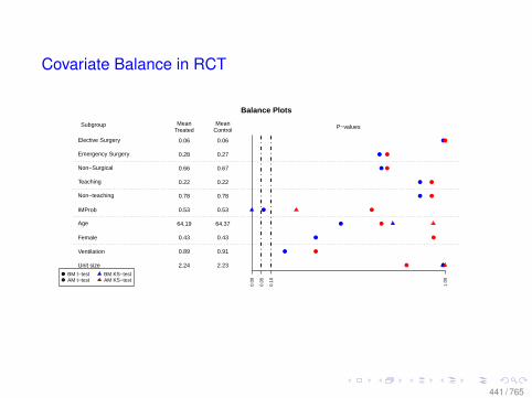
Covariate Balance in RCT
Balance Plots
0.00
0.05
0.10
1.00
MeanTreated
MeanControl P−valuesSubgroup
Elective Surgery 0.06 0.06
Emergency Surgery 0.28 0.27
Non−Surgical 0.66 0.67
Teaching 0.22 0.22
Non−teaching 0.78 0.78
IMProb 0.53 0.53
Age 64.19 64.37
Female 0.43 0.43
Ventilation 0.89 0.91
Unit size 2.24 2.23
BM t−testAM t−test
BM KS−testAM KS−test
441 / 765
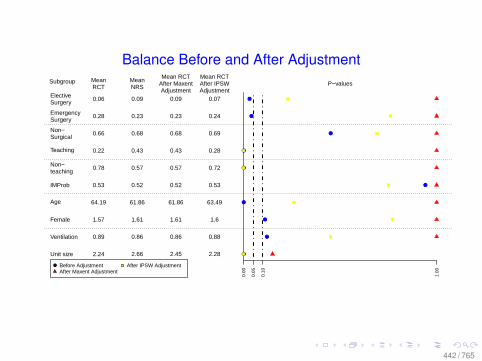
Balance Before and After Adjustment
0.00
0.05
0.10
1.00
MeanRCT
MeanNRS
Mean RCTAfter MaxentAdjustment
Mean RCTAfter IPSWAdjustment
P−valuesSubgroup
ElectiveSurgery
0.06 0.09 0.09 0.07
EmergencySurgery
0.28 0.23 0.23 0.24
Non−Surgical
0.66 0.68 0.68 0.69
Teaching 0.22 0.43 0.43 0.28
Non−teaching
0.78 0.57 0.57 0.72
IMProb 0.53 0.52 0.52 0.53
Age 64.19 61.86 61.86 63.49
Female 1.57 1.61 1.61 1.6
Ventilation 0.89 0.86 0.86 0.88
Unit size 2.24 2.66 2.45 2.28
Before AdjustmentAfter Maxent Adjustment
After IPSW Adjustment
442 / 765
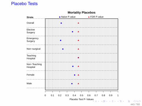
Placebo Tests
0 0.1 0.2 0.3 0.4 0.5 0.6 0.7 0.8 0.9 1
Strata
Mortality PlacebosNaive P.value FDR P.value
Placebo Test P−Values
Male
Female
Non−TeachingHospital
TeachingHospital
Non−surgical
EmergencySurgery
ElectiveSurgery
Overall
443 / 765
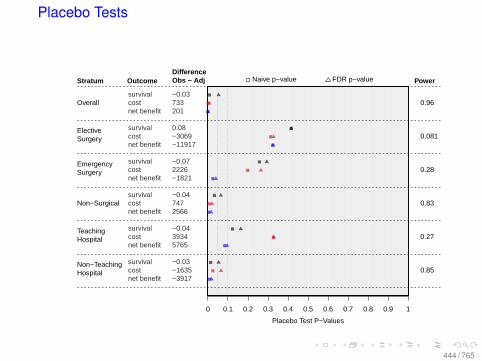
Placebo Tests
0 0.1 0.2 0.3 0.4 0.5 0.6 0.7 0.8 0.9 1
Stratum PowerNaive p−value FDR p−value
Placebo Test P−Values
Non−TeachingHospital 0.85
−3917net benefit−1635cost−0.03survival
TeachingHospital 0.27
5765net benefit3934cost−0.04survival
Non−Surgical 0.832566net benefit747cost−0.04survival
EmergencySurgery 0.28
−1821net benefit2226cost−0.07survival
ElectiveSurgery 0.081
−11917net benefit−3069cost0.08survival
Overall 0.96201net benefit733cost−0.03survival
OutcomeDifferenceObs − Adj
444 / 765
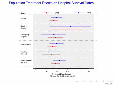
Population Treatment Effects on Hospital Survival Rates
−0.4 −0.2 0 0.2 0.4 0.6
Strata PATT SATT
Treatment Effect EstimatesEffect on Survival Rate (% points)
Non−TeachingHospital
TeachingHospital
Non−Surgical
EmergencySurgery
ElectiveSurgery
Overall
445 / 765
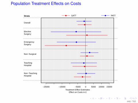
Population Treatment Effects on Costs
−25000 −15000 −5000 0 5000 10000 15000
Strata PATT SATT
Treatment Effect EstimatesEffect on Costs in £
Non−TeachingHospital
TeachingHospital
Non−Surgical
EmergencySurgery
ElectiveSurgery
Overall
446 / 765
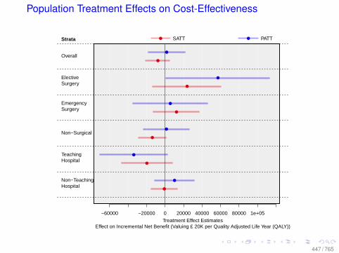
Population Treatment Effects on Cost-Effectiveness
−60000 −20000 0 20000 40000 60000 80000 1e+05
Strata PATT SATT
Treatment Effect EstimatesEffect on Incremental Net Benefit (Valuing £ 20K per Quality Adjusted Life Year (QALY))
Non−TeachingHospital
TeachingHospital
Non−Surgical
EmergencySurgery
ElectiveSurgery
Overall
447 / 765

Conclusions and Implications
• We pass placebo tests for both costs and hospital mortality,thus validating our identifying assumptions for the PATT.
• This has implications for Cost-Effectiveness Analysessince CEAs are often based on observational studies
448 / 765
• See Hartman et al., forthcoming: [LINK]• See the references in that paper on Maximum Entropy
weighting methods. These are also used in SyntheticMatching—i.e., Abadie, Diamond, and Hainmueller, 2010;Hainmueller, 2012
449 / 765
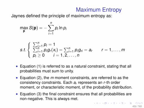
Maximum EntropyJaynes defined the principle of maximum entropy as:
maxp
S(p) = −n∑
i=1
pi ln pi
s.t .
∑n
i=1 pi = 1∑ni=1 pigr (xi) =
∑ni=1 pigri = ar r = 1, . . . ,m
pi ≥ 0 i = 1,2, . . . ,n
• Equation (1) is referred to as a natural constraint, stating that allprobabilities must sum to unity.
• Equation (2), the m moment constraints, are referred to as theconsistency constraints. Each ar represents an r -th ordermoment, or characteristic moment, of the probability distribution.
• Equation (3) the final constraint ensures that all probabilities arenon-negative. This is always met.
450 / 765

Balance Tests and the PropensityScore
Any given propensity score model may not be very good atbalancing the X covariates. After matching on the pscore weneed to test if the underlying X covariates have actually beenbalanced. You need to test more than just balance of thepscore.The MatchBalance() function in Matching provides a numberof tests, the two main ones being the t-test and theKolmogorov-Smirnov Test—the KS test.The KS test tries to determine if two distributions differsignificantly. The KS-test has the advantage of making noassumption about the distribution of data—i.e., it is distributionfree and non-parametric. However, because of this generality,other tests, such as the t-test, are more sensitive to certaindifferences—e.g., mean differences.
451 / 765
Balance Tests and the PropensityScore
Any given propensity score model may not be very good atbalancing the X covariates. After matching on the pscore weneed to test if the underlying X covariates have actually beenbalanced. You need to test more than just balance of thepscore.The MatchBalance() function in Matching provides a numberof tests, the two main ones being the t-test and theKolmogorov-Smirnov Test—the KS test.The KS test tries to determine if two distributions differsignificantly. The KS-test has the advantage of making noassumption about the distribution of data—i.e., it is distributionfree and non-parametric. However, because of this generality,other tests, such as the t-test, are more sensitive to certaindifferences—e.g., mean differences.
452 / 765
Balance Tests and the PropensityScore
Any given propensity score model may not be very good atbalancing the X covariates. After matching on the pscore weneed to test if the underlying X covariates have actually beenbalanced. You need to test more than just balance of thepscore.The MatchBalance() function in Matching provides a numberof tests, the two main ones being the t-test and theKolmogorov-Smirnov Test—the KS test.The KS test tries to determine if two distributions differsignificantly. The KS-test has the advantage of making noassumption about the distribution of data—i.e., it is distributionfree and non-parametric. However, because of this generality,other tests, such as the t-test, are more sensitive to certaindifferences—e.g., mean differences.
453 / 765
KS Test Details and Example
A great description of the standard KS test of offered at thiswebpage: http://www.physics.csbsju.edu/stats/KS-test.html.But the standard KS test does not provide the correct p-valuefor noncontinous variables. But the bootstrap KS does providethe correct p-values. And additional problem arises if we wantto test if distribution from estimated propensity scores differ. Wethen need to do another bootstrap to take into account thedistributions of the parameters in the propensity model.
Also seehttp://sekhon.berkeley.edu/causalinf/R/ks1.R
454 / 765
KS Test Details and Example
A great description of the standard KS test of offered at thiswebpage: http://www.physics.csbsju.edu/stats/KS-test.html.But the standard KS test does not provide the correct p-valuefor noncontinous variables. But the bootstrap KS does providethe correct p-values. And additional problem arises if we wantto test if distribution from estimated propensity scores differ. Wethen need to do another bootstrap to take into account thedistributions of the parameters in the propensity model.
Also seehttp://sekhon.berkeley.edu/causalinf/R/ks1.R
455 / 765
The Bootstrap
Bootstrap methods are a good way of obtaining confidenceintervals and other statistical estimates which require generallyweaker assumptions than the usual analytical approaches.The bootstrap is also useful when we don’t know of ananalytical solution. We lack such solutions when:
1 we are using complicated statistics for which a samplingdistribution is difficult to solve, such as two step estimators
2 we don’t want to make population assumptions
456 / 765
The Bootstrap
Bootstrap methods are a good way of obtaining confidenceintervals and other statistical estimates which require generallyweaker assumptions than the usual analytical approaches.The bootstrap is also useful when we don’t know of ananalytical solution. We lack such solutions when:
1 we are using complicated statistics for which a samplingdistribution is difficult to solve, such as two step estimators
2 we don’t want to make population assumptions
457 / 765
The Bootstrap
Bootstrap methods are a good way of obtaining confidenceintervals and other statistical estimates which require generallyweaker assumptions than the usual analytical approaches.The bootstrap is also useful when we don’t know of ananalytical solution. We lack such solutions when:
1 we are using complicated statistics for which a samplingdistribution is difficult to solve, such as two step estimators
2 we don’t want to make population assumptions
458 / 765
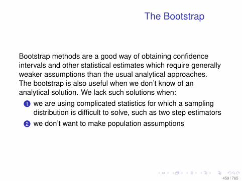
The Bootstrap
Bootstrap methods are a good way of obtaining confidenceintervals and other statistical estimates which require generallyweaker assumptions than the usual analytical approaches.The bootstrap is also useful when we don’t know of ananalytical solution. We lack such solutions when:
1 we are using complicated statistics for which a samplingdistribution is difficult to solve, such as two step estimators
2 we don’t want to make population assumptions
459 / 765
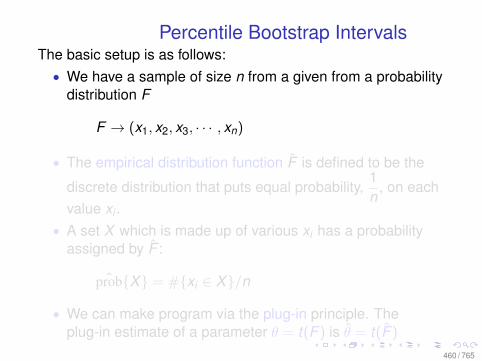
Percentile Bootstrap IntervalsThe basic setup is as follows:• We have a sample of size n from a given from a probability
distribution F
F → (x1, x2, x3, · · · , xn)
• The empirical distribution function F is defined to be the
discrete distribution that puts equal probability,1n
, on eachvalue xi .
• A set X which is made up of various xi has a probabilityassigned by F :
ˆprobX = #xi ∈ X/n
• We can make program via the plug-in principle. Theplug-in estimate of a parameter θ = t(F ) is θ = t(F )
460 / 765
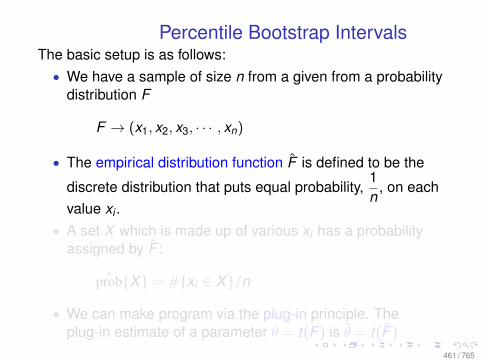
Percentile Bootstrap IntervalsThe basic setup is as follows:• We have a sample of size n from a given from a probability
distribution F
F → (x1, x2, x3, · · · , xn)
• The empirical distribution function F is defined to be the
discrete distribution that puts equal probability,1n
, on eachvalue xi .
• A set X which is made up of various xi has a probabilityassigned by F :
ˆprobX = #xi ∈ X/n
• We can make program via the plug-in principle. Theplug-in estimate of a parameter θ = t(F ) is θ = t(F )
461 / 765
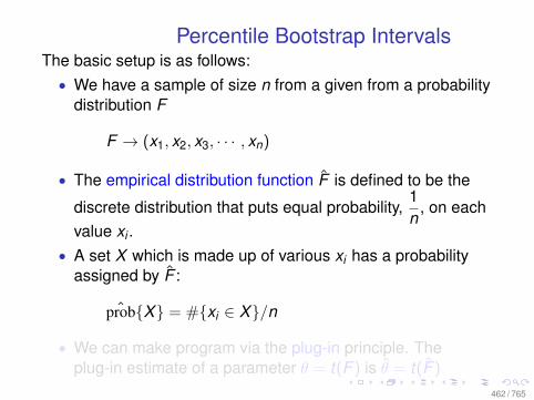
Percentile Bootstrap IntervalsThe basic setup is as follows:• We have a sample of size n from a given from a probability
distribution F
F → (x1, x2, x3, · · · , xn)
• The empirical distribution function F is defined to be the
discrete distribution that puts equal probability,1n
, on eachvalue xi .
• A set X which is made up of various xi has a probabilityassigned by F :
ˆprobX = #xi ∈ X/n
• We can make program via the plug-in principle. Theplug-in estimate of a parameter θ = t(F ) is θ = t(F )
462 / 765
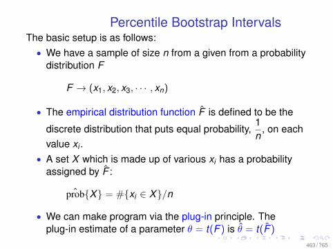
Percentile Bootstrap IntervalsThe basic setup is as follows:• We have a sample of size n from a given from a probability
distribution F
F → (x1, x2, x3, · · · , xn)
• The empirical distribution function F is defined to be the
discrete distribution that puts equal probability,1n
, on eachvalue xi .
• A set X which is made up of various xi has a probabilityassigned by F :
ˆprobX = #xi ∈ X/n
• We can make program via the plug-in principle. Theplug-in estimate of a parameter θ = t(F ) is θ = t(F )
463 / 765
Bootstrap Intervals Algorithm
• For a dataset (denoted “full sample”) iterate the following Btimes where B is a large number such as 1,000.
1 Generate a random sample of size n from x1, · · · , xn withreplacement. This is called a bootstrap sample.
2 calculate the statistic of interest using this bootstrapsample, denoted θb.
• The confidence interval for θ (our full sample estimate) isobtained by taking the quantiles from the samplingdistribution in our bootstrap samples: θb.
• For example, for 95% CI, calculate the 2.5% and 97.5%quantiles of the distribution of θb.
464 / 765

Bootstrap Intervals Algorithm
• For a dataset (denoted “full sample”) iterate the following Btimes where B is a large number such as 1,000.
1 Generate a random sample of size n from x1, · · · , xn withreplacement. This is called a bootstrap sample.
2 calculate the statistic of interest using this bootstrapsample, denoted θb.
• The confidence interval for θ (our full sample estimate) isobtained by taking the quantiles from the samplingdistribution in our bootstrap samples: θb.
• For example, for 95% CI, calculate the 2.5% and 97.5%quantiles of the distribution of θb.
465 / 765
Bootstrap Intervals Algorithm
• For a dataset (denoted “full sample”) iterate the following Btimes where B is a large number such as 1,000.
1 Generate a random sample of size n from x1, · · · , xn withreplacement. This is called a bootstrap sample.
2 calculate the statistic of interest using this bootstrapsample, denoted θb.
• The confidence interval for θ (our full sample estimate) isobtained by taking the quantiles from the samplingdistribution in our bootstrap samples: θb.
• For example, for 95% CI, calculate the 2.5% and 97.5%quantiles of the distribution of θb.
466 / 765
Bootstrap Intervals Algorithm
• For a dataset (denoted “full sample”) iterate the following Btimes where B is a large number such as 1,000.
1 Generate a random sample of size n from x1, · · · , xn withreplacement. This is called a bootstrap sample.
2 calculate the statistic of interest using this bootstrapsample, denoted θb.
• The confidence interval for θ (our full sample estimate) isobtained by taking the quantiles from the samplingdistribution in our bootstrap samples: θb.
• For example, for 95% CI, calculate the 2.5% and 97.5%quantiles of the distribution of θb.
467 / 765
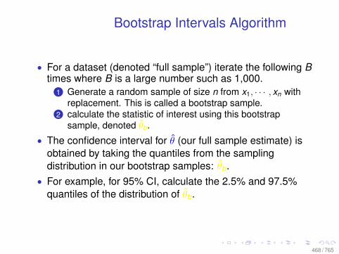
Bootstrap Intervals Algorithm
• For a dataset (denoted “full sample”) iterate the following Btimes where B is a large number such as 1,000.
1 Generate a random sample of size n from x1, · · · , xn withreplacement. This is called a bootstrap sample.
2 calculate the statistic of interest using this bootstrapsample, denoted θb.
• The confidence interval for θ (our full sample estimate) isobtained by taking the quantiles from the samplingdistribution in our bootstrap samples: θb.
• For example, for 95% CI, calculate the 2.5% and 97.5%quantiles of the distribution of θb.
468 / 765
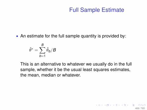
Full Sample Estimate
• An estimate for the full sample quantity is provided by:
θ∗ =B∑
b=1
θb/B
This is an alternative to whatever we usually do in the fullsample, whether it be the usual least squares estimates,the mean, median or whatever.
469 / 765
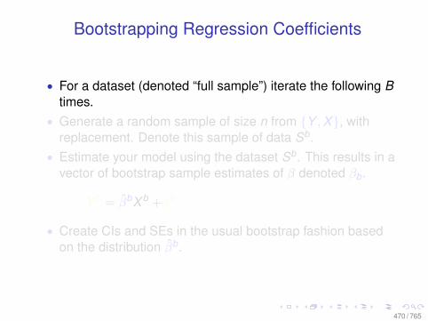
Bootstrapping Regression Coefficients
• For a dataset (denoted “full sample”) iterate the following Btimes.
• Generate a random sample of size n from Y ,X, withreplacement. Denote this sample of data Sb.
• Estimate your model using the dataset Sb. This results in avector of bootstrap sample estimates of β denoted βb.
Y b = βbX b + εb
• Create CIs and SEs in the usual bootstrap fashion basedon the distribution βb.
470 / 765
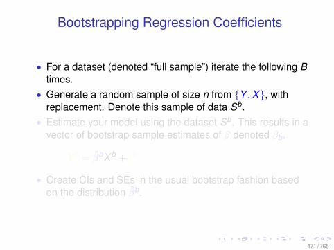
Bootstrapping Regression Coefficients
• For a dataset (denoted “full sample”) iterate the following Btimes.
• Generate a random sample of size n from Y ,X, withreplacement. Denote this sample of data Sb.
• Estimate your model using the dataset Sb. This results in avector of bootstrap sample estimates of β denoted βb.
Y b = βbX b + εb
• Create CIs and SEs in the usual bootstrap fashion basedon the distribution βb.
471 / 765
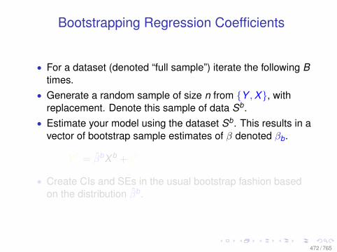
Bootstrapping Regression Coefficients
• For a dataset (denoted “full sample”) iterate the following Btimes.
• Generate a random sample of size n from Y ,X, withreplacement. Denote this sample of data Sb.
• Estimate your model using the dataset Sb. This results in avector of bootstrap sample estimates of β denoted βb.
Y b = βbX b + εb
• Create CIs and SEs in the usual bootstrap fashion basedon the distribution βb.
472 / 765
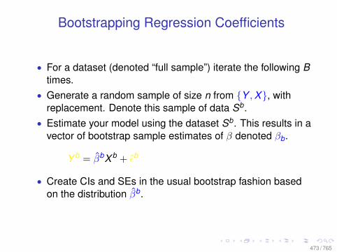
Bootstrapping Regression Coefficients
• For a dataset (denoted “full sample”) iterate the following Btimes.
• Generate a random sample of size n from Y ,X, withreplacement. Denote this sample of data Sb.
• Estimate your model using the dataset Sb. This results in avector of bootstrap sample estimates of β denoted βb.
Y b = βbX b + εb
• Create CIs and SEs in the usual bootstrap fashion basedon the distribution βb.
473 / 765
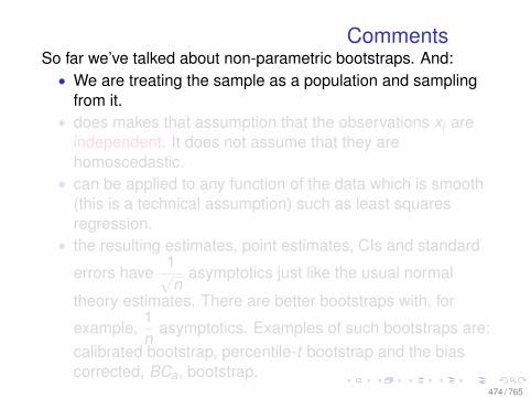
CommentsSo far we’ve talked about non-parametric bootstraps. And:• We are treating the sample as a population and sampling
from it.• does makes that assumption that the observations xi are
independent. It does not assume that they arehomoscedastic.
• can be applied to any function of the data which is smooth(this is a technical assumption) such as least squaresregression.
• the resulting estimates, point estimates, CIs and standard
errors have1√n
asymptotics just like the usual normal
theory estimates. There are better bootstraps with, for
example,1n
asymptotics. Examples of such bootstraps are:calibrated bootstrap, percentile-t bootstrap and the biascorrected, BCa, bootstrap.
474 / 765
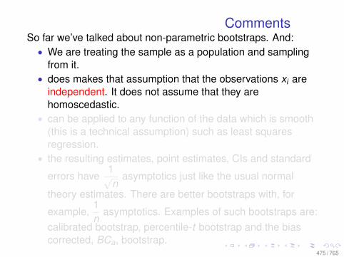
CommentsSo far we’ve talked about non-parametric bootstraps. And:• We are treating the sample as a population and sampling
from it.• does makes that assumption that the observations xi are
independent. It does not assume that they arehomoscedastic.
• can be applied to any function of the data which is smooth(this is a technical assumption) such as least squaresregression.
• the resulting estimates, point estimates, CIs and standard
errors have1√n
asymptotics just like the usual normal
theory estimates. There are better bootstraps with, for
example,1n
asymptotics. Examples of such bootstraps are:calibrated bootstrap, percentile-t bootstrap and the biascorrected, BCa, bootstrap.
475 / 765
CommentsSo far we’ve talked about non-parametric bootstraps. And:• We are treating the sample as a population and sampling
from it.• does makes that assumption that the observations xi are
independent. It does not assume that they arehomoscedastic.
• can be applied to any function of the data which is smooth(this is a technical assumption) such as least squaresregression.
• the resulting estimates, point estimates, CIs and standard
errors have1√n
asymptotics just like the usual normal
theory estimates. There are better bootstraps with, for
example,1n
asymptotics. Examples of such bootstraps are:calibrated bootstrap, percentile-t bootstrap and the biascorrected, BCa, bootstrap.
476 / 765
CommentsSo far we’ve talked about non-parametric bootstraps. And:• We are treating the sample as a population and sampling
from it.• does makes that assumption that the observations xi are
independent. It does not assume that they arehomoscedastic.
• can be applied to any function of the data which is smooth(this is a technical assumption) such as least squaresregression.
• the resulting estimates, point estimates, CIs and standard
errors have1√n
asymptotics just like the usual normal
theory estimates. There are better bootstraps with, for
example,1n
asymptotics. Examples of such bootstraps are:calibrated bootstrap, percentile-t bootstrap and the biascorrected, BCa, bootstrap.
477 / 765
Distributions of Difficult to HandleQuantities
The bootstrap provides an easy way to to obtain the samplingdistribution of quantities for which it is often not known ordifficult to obtain sampling distributions. For example:
• CIs for the median or other quantiles• CIs and SEs for LMS coefficients• In a regression, is β1 > β2
• In a regression, isβ1
β2<β3
β4• Two stage regression estimation. Say a logit in the first
stage and a linear model in the second.• Goodness-of-fit for two model which may not be nested.
478 / 765
Distributions of Difficult to HandleQuantities
The bootstrap provides an easy way to to obtain the samplingdistribution of quantities for which it is often not known ordifficult to obtain sampling distributions. For example:
• CIs for the median or other quantiles• CIs and SEs for LMS coefficients• In a regression, is β1 > β2
• In a regression, isβ1
β2<β3
β4• Two stage regression estimation. Say a logit in the first
stage and a linear model in the second.• Goodness-of-fit for two model which may not be nested.
479 / 765
Distributions of Difficult to HandleQuantities
The bootstrap provides an easy way to to obtain the samplingdistribution of quantities for which it is often not known ordifficult to obtain sampling distributions. For example:
• CIs for the median or other quantiles• CIs and SEs for LMS coefficients• In a regression, is β1 > β2
• In a regression, isβ1
β2<β3
β4• Two stage regression estimation. Say a logit in the first
stage and a linear model in the second.• Goodness-of-fit for two model which may not be nested.
480 / 765
Distributions of Difficult to HandleQuantities
The bootstrap provides an easy way to to obtain the samplingdistribution of quantities for which it is often not known ordifficult to obtain sampling distributions. For example:
• CIs for the median or other quantiles• CIs and SEs for LMS coefficients• In a regression, is β1 > β2
• In a regression, isβ1
β2<β3
β4• Two stage regression estimation. Say a logit in the first
stage and a linear model in the second.• Goodness-of-fit for two model which may not be nested.
481 / 765
Distributions of Difficult to HandleQuantities
The bootstrap provides an easy way to to obtain the samplingdistribution of quantities for which it is often not known ordifficult to obtain sampling distributions. For example:
• CIs for the median or other quantiles• CIs and SEs for LMS coefficients• In a regression, is β1 > β2
• In a regression, isβ1
β2<β3
β4• Two stage regression estimation. Say a logit in the first
stage and a linear model in the second.• Goodness-of-fit for two model which may not be nested.
482 / 765
Distributions of Difficult to HandleQuantities
The bootstrap provides an easy way to to obtain the samplingdistribution of quantities for which it is often not known ordifficult to obtain sampling distributions. For example:
• CIs for the median or other quantiles• CIs and SEs for LMS coefficients• In a regression, is β1 > β2
• In a regression, isβ1
β2<β3
β4• Two stage regression estimation. Say a logit in the first
stage and a linear model in the second.• Goodness-of-fit for two model which may not be nested.
483 / 765
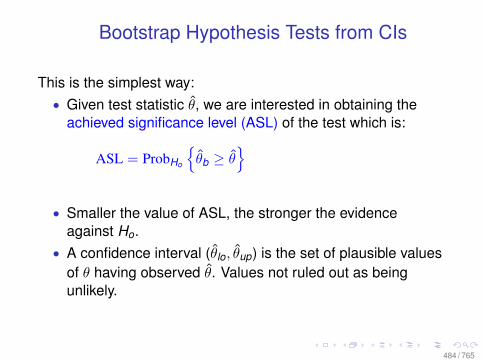
Bootstrap Hypothesis Tests from CIs
This is the simplest way:• Given test statistic θ, we are interested in obtaining the
achieved significance level (ASL) of the test which is:
ASL = ProbHo
θb ≥ θ
• Smaller the value of ASL, the stronger the evidenceagainst Ho.
• A confidence interval (θlo, θup) is the set of plausible valuesof θ having observed θ. Values not ruled out as beingunlikely.
484 / 765
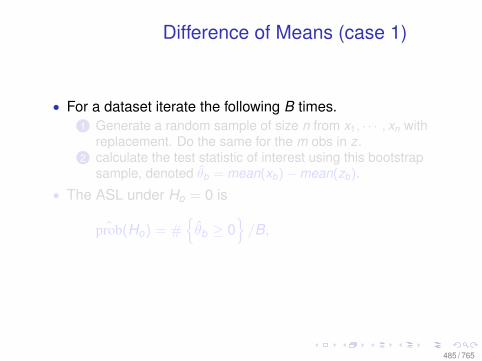
Difference of Means (case 1)
• For a dataset iterate the following B times.1 Generate a random sample of size n from x1, · · · , xn with
replacement. Do the same for the m obs in z.2 calculate the test statistic of interest using this bootstrap
sample, denoted θb = mean(xb)−mean(zb).
• The ASL under Ho = 0 is
ˆprob(Ho) = #θb ≥ 0
/B,
485 / 765
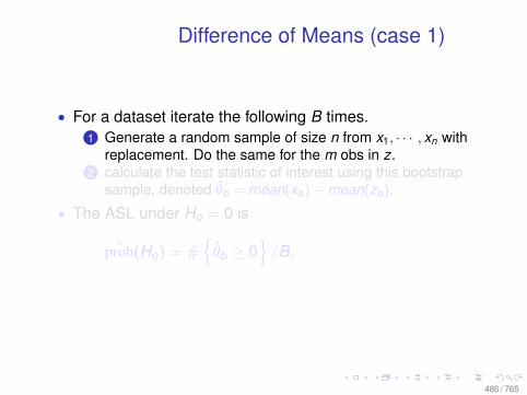
Difference of Means (case 1)
• For a dataset iterate the following B times.1 Generate a random sample of size n from x1, · · · , xn with
replacement. Do the same for the m obs in z.2 calculate the test statistic of interest using this bootstrap
sample, denoted θb = mean(xb)−mean(zb).
• The ASL under Ho = 0 is
ˆprob(Ho) = #θb ≥ 0
/B,
486 / 765
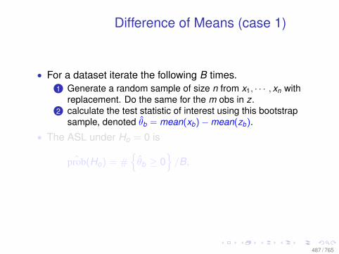
Difference of Means (case 1)
• For a dataset iterate the following B times.1 Generate a random sample of size n from x1, · · · , xn with
replacement. Do the same for the m obs in z.2 calculate the test statistic of interest using this bootstrap
sample, denoted θb = mean(xb)−mean(zb).
• The ASL under Ho = 0 is
ˆprob(Ho) = #θb ≥ 0
/B,
487 / 765
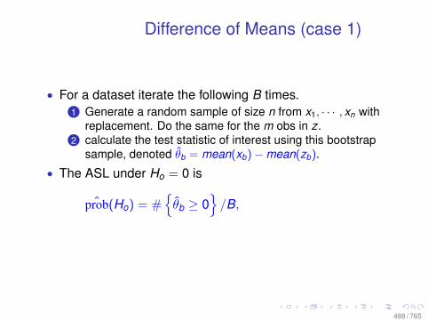
Difference of Means (case 1)
• For a dataset iterate the following B times.1 Generate a random sample of size n from x1, · · · , xn with
replacement. Do the same for the m obs in z.2 calculate the test statistic of interest using this bootstrap
sample, denoted θb = mean(xb)−mean(zb).
• The ASL under Ho = 0 is
ˆprob(Ho) = #θb ≥ 0
/B,
488 / 765
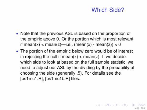
Which Side?
• Note that the previous ASL is based on the proportion ofthe empiric above 0. Or the portion which is most relevantif mean(x) < mean(z)—i.e., (mean(x) - mean(z)) < 0
• The portion of the empiric below zero would be of interestin rejecting the null if mean(x) > mean(z). If we decidewhich side to look at based on the full sample statistic, weneed to adjust our ASL by the dividing by the probability ofchoosing the side (generally .5). For details see the[bs1mc1.R], [bs1mc1b.R] files.
489 / 765
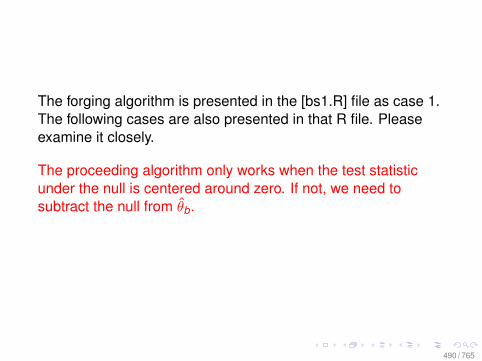
The forging algorithm is presented in the [bs1.R] file as case 1.The following cases are also presented in that R file. Pleaseexamine it closely.
The proceeding algorithm only works when the test statisticunder the null is centered around zero. If not, we need tosubtract the null from θb.
490 / 765
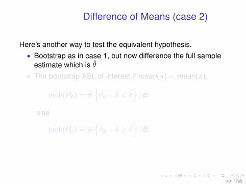
Difference of Means (case 2)
Here’s another way to test the equivalent hypothesis.• Bootstrap as in case 1, but now difference the full sample
estimate which is θ• The bootstrap ASL of interest if mean(x) < mean(z),
ˆprob(Ho) = #θb − θ < θ
/B,
else
ˆprob(Ho) = #θb − θ ≥ θ
/B,
491 / 765
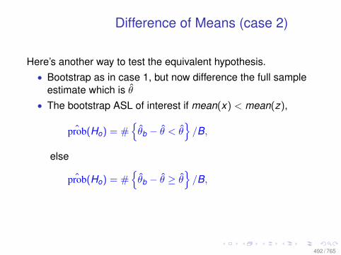
Difference of Means (case 2)
Here’s another way to test the equivalent hypothesis.• Bootstrap as in case 1, but now difference the full sample
estimate which is θ• The bootstrap ASL of interest if mean(x) < mean(z),
ˆprob(Ho) = #θb − θ < θ
/B,
else
ˆprob(Ho) = #θb − θ ≥ θ
/B,
492 / 765
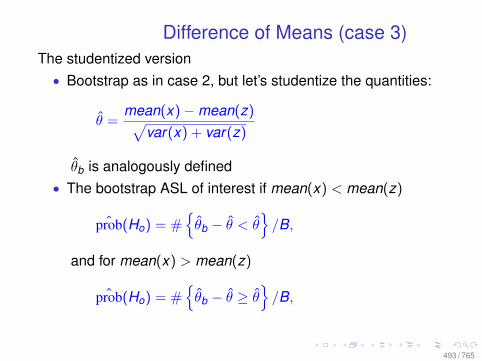
Difference of Means (case 3)The studentized version• Bootstrap as in case 2, but let’s studentize the quantities:
θ =mean(x)−mean(z)√
var(x) + var(z)
θb is analogously defined• The bootstrap ASL of interest if mean(x) < mean(z)
ˆprob(Ho) = #θb − θ < θ
/B,
and for mean(x) > mean(z)
ˆprob(Ho) = #θb − θ ≥ θ
/B,
493 / 765
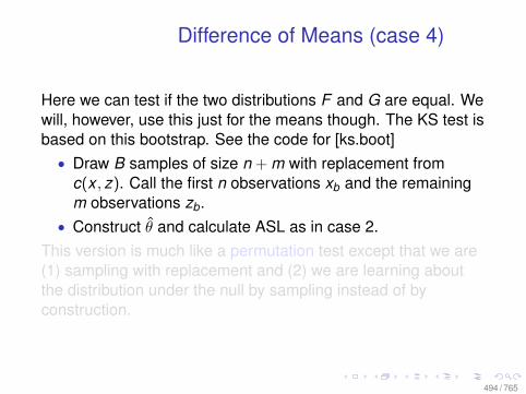
Difference of Means (case 4)
Here we can test if the two distributions F and G are equal. Wewill, however, use this just for the means though. The KS test isbased on this bootstrap. See the code for [ks.boot]• Draw B samples of size n + m with replacement from
c(x , z). Call the first n observations xb and the remainingm observations zb.
• Construct θ and calculate ASL as in case 2.This version is much like a permutation test except that we are(1) sampling with replacement and (2) we are learning aboutthe distribution under the null by sampling instead of byconstruction.
494 / 765
Difference of Means (case 4)
Here we can test if the two distributions F and G are equal. Wewill, however, use this just for the means though. The KS test isbased on this bootstrap. See the code for [ks.boot]• Draw B samples of size n + m with replacement from
c(x , z). Call the first n observations xb and the remainingm observations zb.
• Construct θ and calculate ASL as in case 2.This version is much like a permutation test except that we are(1) sampling with replacement and (2) we are learning aboutthe distribution under the null by sampling instead of byconstruction.
495 / 765
Different Null Hypothesizes
• Code which adapts case four to use the KS test is providedat: [bs2.R]
• All four cases are based on the null hypothesis that themeans in the two samples are equal. The null hypothesisneed not be so restrictive for the first three cases.
• Why in the fourth case doesn’t non-equality make sense?We could generalize (much like a sharp null).
• The following cases generalize the first three cases for thenon-zero difference setting. For R code see: [bs1_null.R].
496 / 765
Difference of Means Redux (case 1∗)
• Bootstrap as before. Note that the null hypothesis is H0
• The bootstrap ASL of interest if[mean(x)−mean(z)] < H0, is
ˆprob(Ho) = #θb ≥ H0
/B,
else
ˆprob(Ho) = #θb < H0
/B.
497 / 765
Difference of Means Redux (case 1∗)
• Bootstrap as before. Note that the null hypothesis is H0
• The bootstrap ASL of interest if[mean(x)−mean(z)] < H0, is
ˆprob(Ho) = #θb ≥ H0
/B,
else
ˆprob(Ho) = #θb < H0
/B.
498 / 765
Difference of Means Redux (case 2∗)
• Bootstrap as before.• The bootstrap ASL of interest if
[mean(x)−mean(z)] < H0, is
ˆprob(Ho) = #θb − θ < θ − H0
/B,
else
ˆprob(Ho) = #θb − θ ≥ θ − H0
/B,
499 / 765
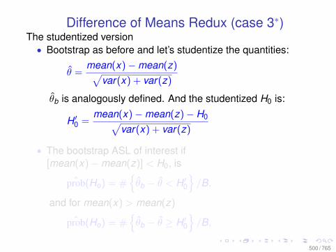
Difference of Means Redux (case 3∗)The studentized version• Bootstrap as before and let’s studentize the quantities:
θ =mean(x)−mean(z)√
var(x) + var(z)
θb is analogously defined. And the studentized H0 is:
H ′0 =mean(x)−mean(z)− H0√
var(x) + var(z)
• The bootstrap ASL of interest if[mean(x)−mean(z)] < H0, is
ˆprob(Ho) = #θb − θ < H ′0
/B,
and for mean(x) > mean(z)
ˆprob(Ho) = #θb − θ ≥ H ′0
/B,
500 / 765
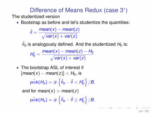
Difference of Means Redux (case 3∗)The studentized version• Bootstrap as before and let’s studentize the quantities:
θ =mean(x)−mean(z)√
var(x) + var(z)
θb is analogously defined. And the studentized H0 is:
H ′0 =mean(x)−mean(z)− H0√
var(x) + var(z)
• The bootstrap ASL of interest if[mean(x)−mean(z)] < H0, is
ˆprob(Ho) = #θb − θ < H ′0
/B,
and for mean(x) > mean(z)
ˆprob(Ho) = #θb − θ ≥ H ′0
/B,
501 / 765
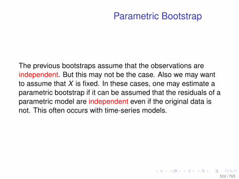
Parametric Bootstrap
The previous bootstraps assume that the observations areindependent. But this may not be the case. Also we may wantto assume that X is fixed. In these cases, one may estimate aparametric bootstrap if it can be assumed that the residuals of aparametric model are independent even if the original data isnot. This often occurs with time-series models.
502 / 765
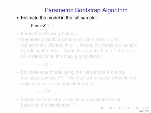
Parametric Bootstrap Algorithm• Estimate the model in the full-sample:
Y = βX + ε
• Iterate the following B times.• Generate a random sample of size n from ε, with
replacement. Denote this εb. Create the bootstrap sampleby adding the new εb to the full sample X and β (there isNO estimation in this step, just addition):
Y b = βX + εb
• Estimate your model using the full sample X but thebootstrap sample Y b. This results in a vector of bootstrapestimates of β estimates denoted βb.
Y b = βbX + εb
• Create CIs and SEs in the usual bootstrap fashionbased on the distribution βb.
503 / 765
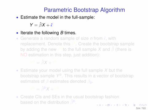
Parametric Bootstrap Algorithm• Estimate the model in the full-sample:
Y = βX + ε
• Iterate the following B times.• Generate a random sample of size n from ε, with
replacement. Denote this εb. Create the bootstrap sampleby adding the new εb to the full sample X and β (there isNO estimation in this step, just addition):
Y b = βX + εb
• Estimate your model using the full sample X but thebootstrap sample Y b. This results in a vector of bootstrapestimates of β estimates denoted βb.
Y b = βbX + εb
• Create CIs and SEs in the usual bootstrap fashionbased on the distribution βb.
504 / 765
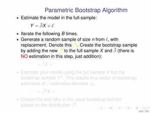
Parametric Bootstrap Algorithm• Estimate the model in the full-sample:
Y = βX + ε
• Iterate the following B times.• Generate a random sample of size n from ε, with
replacement. Denote this εb. Create the bootstrap sampleby adding the new εb to the full sample X and β (there isNO estimation in this step, just addition):
Y b = βX + εb
• Estimate your model using the full sample X but thebootstrap sample Y b. This results in a vector of bootstrapestimates of β estimates denoted βb.
Y b = βbX + εb
• Create CIs and SEs in the usual bootstrap fashionbased on the distribution βb.
505 / 765
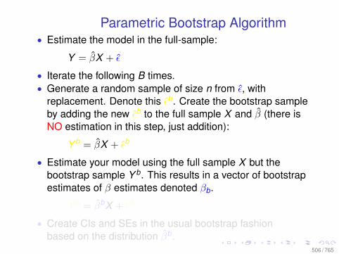
Parametric Bootstrap Algorithm• Estimate the model in the full-sample:
Y = βX + ε
• Iterate the following B times.• Generate a random sample of size n from ε, with
replacement. Denote this εb. Create the bootstrap sampleby adding the new εb to the full sample X and β (there isNO estimation in this step, just addition):
Y b = βX + εb
• Estimate your model using the full sample X but thebootstrap sample Y b. This results in a vector of bootstrapestimates of β estimates denoted βb.
Y b = βbX + εb
• Create CIs and SEs in the usual bootstrap fashionbased on the distribution βb.
506 / 765
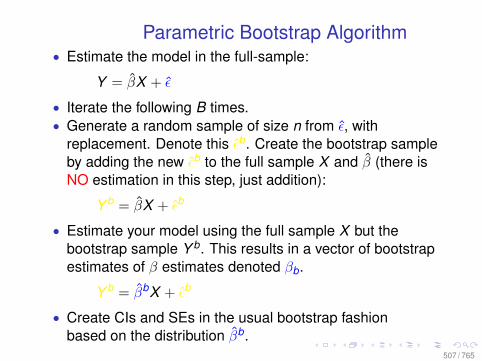
Parametric Bootstrap Algorithm• Estimate the model in the full-sample:
Y = βX + ε
• Iterate the following B times.• Generate a random sample of size n from ε, with
replacement. Denote this εb. Create the bootstrap sampleby adding the new εb to the full sample X and β (there isNO estimation in this step, just addition):
Y b = βX + εb
• Estimate your model using the full sample X but thebootstrap sample Y b. This results in a vector of bootstrapestimates of β estimates denoted βb.
Y b = βbX + εb
• Create CIs and SEs in the usual bootstrap fashionbased on the distribution βb.
507 / 765
Two Nice Bootstrap PropertiesBootstrap CI estimates are:
1 Range Preserving. The confidence interval cannot extendbeyond the range which estimates of θ range in bootstrapsamples. For example, if we are bootstrapping estimates ofa proportion, our confidence interval cannot be less than 0or greater than 1. The usual normal theory confidenceintervals are not range persevering.
2 Take into account more general uncertainty. Manyestimators, such as LMS, have the usual statisticaluncertainty (due to sampling) but also have uncertaintybecause the algorithm used to obtain the estimates isstochastic or otherwise suboptimal. Bootstrap CIs will takethis uncertainty into account. See the R help on the lqsfunction for more information about how the LMS estimatesare obtained.
508 / 765
Two Nice Bootstrap PropertiesBootstrap CI estimates are:
1 Range Preserving. The confidence interval cannot extendbeyond the range which estimates of θ range in bootstrapsamples. For example, if we are bootstrapping estimates ofa proportion, our confidence interval cannot be less than 0or greater than 1. The usual normal theory confidenceintervals are not range persevering.
2 Take into account more general uncertainty. Manyestimators, such as LMS, have the usual statisticaluncertainty (due to sampling) but also have uncertaintybecause the algorithm used to obtain the estimates isstochastic or otherwise suboptimal. Bootstrap CIs will takethis uncertainty into account. See the R help on the lqsfunction for more information about how the LMS estimatesare obtained.
509 / 765

Bootstrap Readings
For bootstrap algorithms see Venables and Ripley (2002).Especially, p.133-138 (section 5.7) and p.163-165 (section 6.6).The R "boot" command is of particular interest.For a statistical discussion see Chapter 16 (p.493ff) of Fox(2002).For additional readings see:
• Efron, Bradley and Tibshirani, Robert J. 1994. AnIntroduction to the Bootstrap. Chapman & Hall. ISBN:0412042312.
• Davison, A. C. and Hinkely, D. V. 1997. Bootstrap Methodsand their Applications. Cambridge University Press.
• Go to jstor and search for Efron and/or Tibshirani.
510 / 765
Bootstrap Readings
For bootstrap algorithms see Venables and Ripley (2002).Especially, p.133-138 (section 5.7) and p.163-165 (section 6.6).The R "boot" command is of particular interest.For a statistical discussion see Chapter 16 (p.493ff) of Fox(2002).For additional readings see:
• Efron, Bradley and Tibshirani, Robert J. 1994. AnIntroduction to the Bootstrap. Chapman & Hall. ISBN:0412042312.
• Davison, A. C. and Hinkely, D. V. 1997. Bootstrap Methodsand their Applications. Cambridge University Press.
• Go to jstor and search for Efron and/or Tibshirani.
511 / 765
Bootstrap Readings
For bootstrap algorithms see Venables and Ripley (2002).Especially, p.133-138 (section 5.7) and p.163-165 (section 6.6).The R "boot" command is of particular interest.For a statistical discussion see Chapter 16 (p.493ff) of Fox(2002).For additional readings see:
• Efron, Bradley and Tibshirani, Robert J. 1994. AnIntroduction to the Bootstrap. Chapman & Hall. ISBN:0412042312.
• Davison, A. C. and Hinkely, D. V. 1997. Bootstrap Methodsand their Applications. Cambridge University Press.
• Go to jstor and search for Efron and/or Tibshirani.
512 / 765
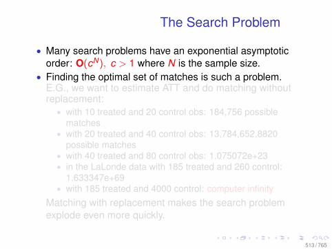
The Search Problem
• Many search problems have an exponential asymptoticorder: O(cN), c > 1 where N is the sample size.
• Finding the optimal set of matches is such a problem.E.G., we want to estimate ATT and do matching withoutreplacement:• with 10 treated and 20 control obs: 184,756 possible
matches• with 20 treated and 40 control obs: 13,784,652,8820
possible matches• with 40 treated and 80 control obs: 1.075072e+23• in the LaLonde data with 185 treated and 260 control:
1.633347e+69• with 185 treated and 4000 control: computer infinity
Matching with replacement makes the search problemexplode even more quickly.
513 / 765
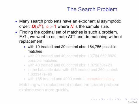
The Search Problem
• Many search problems have an exponential asymptoticorder: O(cN), c > 1 where N is the sample size.
• Finding the optimal set of matches is such a problem.E.G., we want to estimate ATT and do matching withoutreplacement:• with 10 treated and 20 control obs: 184,756 possible
matches• with 20 treated and 40 control obs: 13,784,652,8820
possible matches• with 40 treated and 80 control obs: 1.075072e+23• in the LaLonde data with 185 treated and 260 control:
1.633347e+69• with 185 treated and 4000 control: computer infinity
Matching with replacement makes the search problemexplode even more quickly.
514 / 765
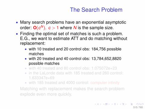
The Search Problem
• Many search problems have an exponential asymptoticorder: O(cN), c > 1 where N is the sample size.
• Finding the optimal set of matches is such a problem.E.G., we want to estimate ATT and do matching withoutreplacement:• with 10 treated and 20 control obs: 184,756 possible
matches• with 20 treated and 40 control obs: 13,784,652,8820
possible matches• with 40 treated and 80 control obs: 1.075072e+23• in the LaLonde data with 185 treated and 260 control:
1.633347e+69• with 185 treated and 4000 control: computer infinity
Matching with replacement makes the search problemexplode even more quickly.
515 / 765
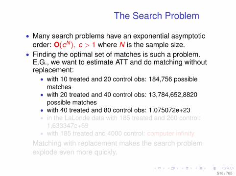
The Search Problem
• Many search problems have an exponential asymptoticorder: O(cN), c > 1 where N is the sample size.
• Finding the optimal set of matches is such a problem.E.G., we want to estimate ATT and do matching withoutreplacement:• with 10 treated and 20 control obs: 184,756 possible
matches• with 20 treated and 40 control obs: 13,784,652,8820
possible matches• with 40 treated and 80 control obs: 1.075072e+23• in the LaLonde data with 185 treated and 260 control:
1.633347e+69• with 185 treated and 4000 control: computer infinity
Matching with replacement makes the search problemexplode even more quickly.
516 / 765
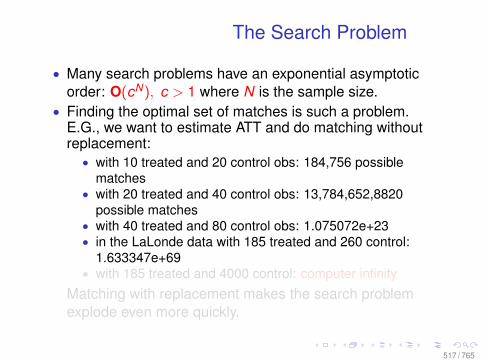
The Search Problem
• Many search problems have an exponential asymptoticorder: O(cN), c > 1 where N is the sample size.
• Finding the optimal set of matches is such a problem.E.G., we want to estimate ATT and do matching withoutreplacement:• with 10 treated and 20 control obs: 184,756 possible
matches• with 20 treated and 40 control obs: 13,784,652,8820
possible matches• with 40 treated and 80 control obs: 1.075072e+23• in the LaLonde data with 185 treated and 260 control:
1.633347e+69• with 185 treated and 4000 control: computer infinity
Matching with replacement makes the search problemexplode even more quickly.
517 / 765
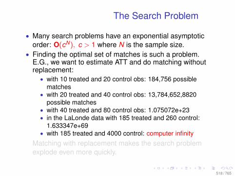
The Search Problem
• Many search problems have an exponential asymptoticorder: O(cN), c > 1 where N is the sample size.
• Finding the optimal set of matches is such a problem.E.G., we want to estimate ATT and do matching withoutreplacement:• with 10 treated and 20 control obs: 184,756 possible
matches• with 20 treated and 40 control obs: 13,784,652,8820
possible matches• with 40 treated and 80 control obs: 1.075072e+23• in the LaLonde data with 185 treated and 260 control:
1.633347e+69• with 185 treated and 4000 control: computer infinity
Matching with replacement makes the search problemexplode even more quickly.
518 / 765
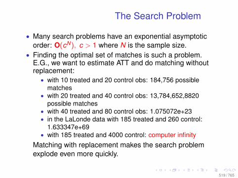
The Search Problem
• Many search problems have an exponential asymptoticorder: O(cN), c > 1 where N is the sample size.
• Finding the optimal set of matches is such a problem.E.G., we want to estimate ATT and do matching withoutreplacement:• with 10 treated and 20 control obs: 184,756 possible
matches• with 20 treated and 40 control obs: 13,784,652,8820
possible matches• with 40 treated and 80 control obs: 1.075072e+23• in the LaLonde data with 185 treated and 260 control:
1.633347e+69• with 185 treated and 4000 control: computer infinity
Matching with replacement makes the search problemexplode even more quickly.
519 / 765
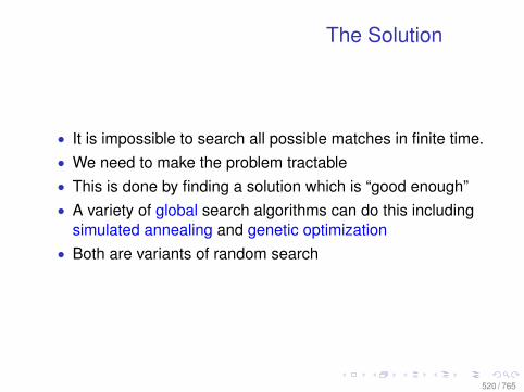
The Solution
• It is impossible to search all possible matches in finite time.• We need to make the problem tractable• This is done by finding a solution which is “good enough”• A variety of global search algorithms can do this including
simulated annealing and genetic optimization• Both are variants of random search
520 / 765
Difficult Optimization Problems
• Loss functions of statistical models are often irregular• ML models are generally not globally concave• As such, deriviative methods fail to find the global
maximum• And Taylor series methods for SEs do not provide correct
coverage
521 / 765

Normal Mixtures
Mixtures of Normal Densities provides a nice way to createdifficult optimization surfaces.
The Claw:
12
N(0,1) +4∑
m=0
110
N(m2− 1, (
110
))
522 / 765
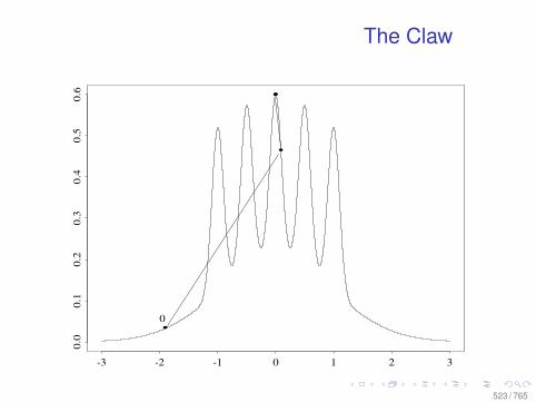
The Claw
-3 -2 -1 0 1 2 3
0.0
0.1
0.2
0.3
0.4
0.5
0.6
•
•
••
0
523 / 765

Normal Mixtures
Asymmetric Double Claw:
1∑m=0
46100
N(2m − 1,23
) +
3∑m=1
1300
N(−m2,
1100
) +
3∑m=1
7300
N(m2,
7100
)
524 / 765
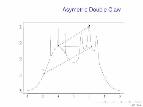
Asymetric Double Claw
-3 -2 -1 0 1 2 3
0.0
0.1
0.2
0.3
0.4
•
••
•••
0
525 / 765
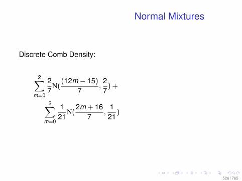
Normal Mixtures
Discrete Comb Density:
2∑m=0
27
N((12m − 15)
7,27
) +
2∑m=0
121
N(2m + 16
7,
121
)
526 / 765
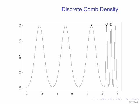
Discrete Comb Density
-3 -2 -1 0 1 2 3
0.0
0.1
0.2
0.3
0.4 •• ••••
0 2431
527 / 765
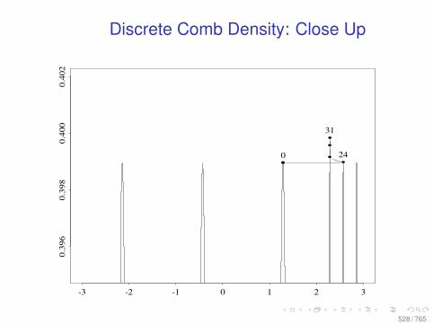
Discrete Comb Density: Close Up
-3 -2 -1 0 1 2 3
0.39
60.
398
0.40
00.
402
•• ••••
0 24
31
528 / 765
Evolutionary Search (EA)
• An EA uses a collection of heuristic rules to modify apopulation of trial solutions in such a way that eachgeneration of trial values tends to be on average betterthan its predecessor.
• The EA in GENOUD assumes a solution is a vector of realnumbers, each number being a value for a scalarparameter of a function to be optimized.
• parameter==gene• Each heuristic rule, or operator, acts on one or more trial
solutions from the current population to produce one ormore trial solutions to be included in the new population.
529 / 765
Evolutionary Search (EA)
• An EA uses a collection of heuristic rules to modify apopulation of trial solutions in such a way that eachgeneration of trial values tends to be on average betterthan its predecessor.
• The EA in GENOUD assumes a solution is a vector of realnumbers, each number being a value for a scalarparameter of a function to be optimized.
• parameter==gene• Each heuristic rule, or operator, acts on one or more trial
solutions from the current population to produce one ormore trial solutions to be included in the new population.
530 / 765
Description
• A GA uses a set of randomized genetic operators to evolvea finite population of finite code-strings over a series ofgenerations (Holland 1975; Goldberg 1989; Grefenstetteand Baker 1989)
• The operators used in GA implementations vary, but thebasic set of operators can be defined as reproduction,mutation and crossover (Davis 1991; Filho, Treleaven andAlippi 1994).
531 / 765
General Description of Operators
• reproduction: a copy of an individual in the currentpopulation is reproduced into the new one. Analogous toasexual reproduction.
• mutation: randomly alter parameter values (genes) so asto search the entire space
• crossover: Create a new individual from one or moreindividuals from the current population. Splice someparameters from individual A with the parameter valuesfrom another individual. Analogous to sexual reproduction.
• All three can be combined to create mixed operators
532 / 765
General Description of Operators
• reproduction: a copy of an individual in the currentpopulation is reproduced into the new one. Analogous toasexual reproduction.
• mutation: randomly alter parameter values (genes) so asto search the entire space
• crossover: Create a new individual from one or moreindividuals from the current population. Splice someparameters from individual A with the parameter valuesfrom another individual. Analogous to sexual reproduction.
• All three can be combined to create mixed operators
533 / 765
General Description of Operators
• reproduction: a copy of an individual in the currentpopulation is reproduced into the new one. Analogous toasexual reproduction.
• mutation: randomly alter parameter values (genes) so asto search the entire space
• crossover: Create a new individual from one or moreindividuals from the current population. Splice someparameters from individual A with the parameter valuesfrom another individual. Analogous to sexual reproduction.
• All three can be combined to create mixed operators
534 / 765
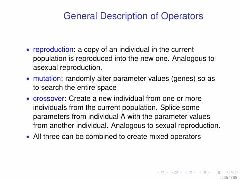
General Description of Operators
• reproduction: a copy of an individual in the currentpopulation is reproduced into the new one. Analogous toasexual reproduction.
• mutation: randomly alter parameter values (genes) so asto search the entire space
• crossover: Create a new individual from one or moreindividuals from the current population. Splice someparameters from individual A with the parameter valuesfrom another individual. Analogous to sexual reproduction.
• All three can be combined to create mixed operators
535 / 765
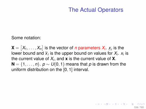
The Actual Operators
Some notation:
X =[X1, . . . ,Xn
]is the vector of n parameters Xi . x i is the
lower bound and x i is the upper bound on values for Xi . xi isthe current value of Xi , and x is the current value of X.N = 1, . . . ,n. p ∼ U(0,1) means that p is drawn from theuniform distribution on the [0,1] interval.
536 / 765
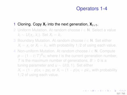
Operators 1-4
1 Cloning. Copy Xt into the next generation, Xt+1.2 Uniform Mutation. At random choose i ∈ N. Select a value
xi ∼ U(x i , x i). Set Xi = xi .3 Boundary Mutation. At random choose i ∈ N. Set either
Xi = x i or Xi = x i , with probability 1/2 of using each value.4 Non-uniform Mutation. At random choose i ∈ N. Compute
p = (1− t/T )Bu, where t is the current generation number,T is the maximum number of generations, B > 0 is atuning parameter and u ∼ U(0,1). Set eitherXi = (1− p)xi + px i or Xi = (1− p)xi + px i , with probability1/2 of using each value.
537 / 765
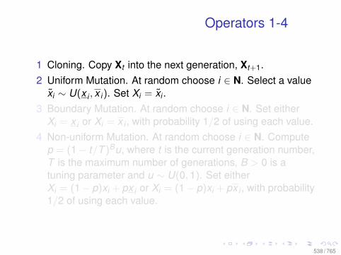
Operators 1-4
1 Cloning. Copy Xt into the next generation, Xt+1.2 Uniform Mutation. At random choose i ∈ N. Select a value
xi ∼ U(x i , x i). Set Xi = xi .3 Boundary Mutation. At random choose i ∈ N. Set either
Xi = x i or Xi = x i , with probability 1/2 of using each value.4 Non-uniform Mutation. At random choose i ∈ N. Compute
p = (1− t/T )Bu, where t is the current generation number,T is the maximum number of generations, B > 0 is atuning parameter and u ∼ U(0,1). Set eitherXi = (1− p)xi + px i or Xi = (1− p)xi + px i , with probability1/2 of using each value.
538 / 765
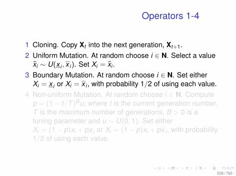
Operators 1-4
1 Cloning. Copy Xt into the next generation, Xt+1.2 Uniform Mutation. At random choose i ∈ N. Select a value
xi ∼ U(x i , x i). Set Xi = xi .3 Boundary Mutation. At random choose i ∈ N. Set either
Xi = x i or Xi = x i , with probability 1/2 of using each value.4 Non-uniform Mutation. At random choose i ∈ N. Compute
p = (1− t/T )Bu, where t is the current generation number,T is the maximum number of generations, B > 0 is atuning parameter and u ∼ U(0,1). Set eitherXi = (1− p)xi + px i or Xi = (1− p)xi + px i , with probability1/2 of using each value.
539 / 765
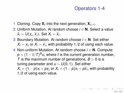
Operators 1-4
1 Cloning. Copy Xt into the next generation, Xt+1.2 Uniform Mutation. At random choose i ∈ N. Select a value
xi ∼ U(x i , x i). Set Xi = xi .3 Boundary Mutation. At random choose i ∈ N. Set either
Xi = x i or Xi = x i , with probability 1/2 of using each value.4 Non-uniform Mutation. At random choose i ∈ N. Compute
p = (1− t/T )Bu, where t is the current generation number,T is the maximum number of generations, B > 0 is atuning parameter and u ∼ U(0,1). Set eitherXi = (1− p)xi + px i or Xi = (1− p)xi + px i , with probability1/2 of using each value.
540 / 765
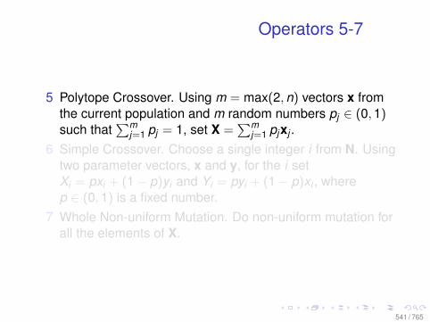
Operators 5-7
5 Polytope Crossover. Using m = max(2,n) vectors x fromthe current population and m random numbers pj ∈ (0,1)such that
∑mj=1 pj = 1, set X =
∑mj=1 pjxj .
6 Simple Crossover. Choose a single integer i from N. Usingtwo parameter vectors, x and y, for the i setXi = pxi + (1− p)yi and Yi = pyi + (1− p)xi , wherep ∈ (0,1) is a fixed number.
7 Whole Non-uniform Mutation. Do non-uniform mutation forall the elements of X.
541 / 765
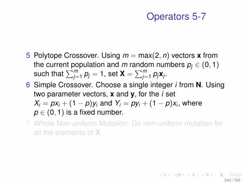
Operators 5-7
5 Polytope Crossover. Using m = max(2,n) vectors x fromthe current population and m random numbers pj ∈ (0,1)such that
∑mj=1 pj = 1, set X =
∑mj=1 pjxj .
6 Simple Crossover. Choose a single integer i from N. Usingtwo parameter vectors, x and y, for the i setXi = pxi + (1− p)yi and Yi = pyi + (1− p)xi , wherep ∈ (0,1) is a fixed number.
7 Whole Non-uniform Mutation. Do non-uniform mutation forall the elements of X.
542 / 765
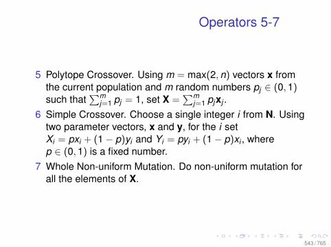
Operators 5-7
5 Polytope Crossover. Using m = max(2,n) vectors x fromthe current population and m random numbers pj ∈ (0,1)such that
∑mj=1 pj = 1, set X =
∑mj=1 pjxj .
6 Simple Crossover. Choose a single integer i from N. Usingtwo parameter vectors, x and y, for the i setXi = pxi + (1− p)yi and Yi = pyi + (1− p)xi , wherep ∈ (0,1) is a fixed number.
7 Whole Non-uniform Mutation. Do non-uniform mutation forall the elements of X.
543 / 765
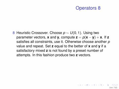
Operators 8
8 Heuristic Crossover. Choose p ∼ U(0,1). Using twoparameter vectors, x and y, compute z = p(x− y) + x. If zsatisfies all constraints, use it. Otherwise choose another pvalue and repeat. Set z equal to the better of x and y if asatisfactory mixed z is not found by a preset number ofattempts. In this fashion produce two z vectors.
544 / 765
Operators 9
9 Local-minimum Crossover. NOT USED IN GENMATCH.Choose p ∼ U(0,1). Starting with x, run BFGSoptimization up to a preset number of iterations to produce~x. Compute z = p~x + (1− p)x. If z satisfies boundaryconstraints, use it. Otherwise shrink p by setting p = p/2and recompute z. If a satisfactory z is not found by apreset number of attempts, return x. This operators isextremely computationally intensive, use sparingly.
545 / 765

Markov Chains
GAs are Markov chains:
A Markov chain describes at successive times the states of a system.At these times the system may have changed from the state it was inthe moment before to another or stayed in the same state. Thechanges of state are called transitions. The Markov property meansthat the conditional probability distribution of the state in the future,given the state of the process currently and in the past, depends onlyon its current state and not on its state in the past.
546 / 765
Markov Chains II
A Markov chain is a sequence of random variablesX1,X2,X3, . . . with the Markov property, that is, given thepresent state, the future state and past states are independent.Formally:
Pr (Xn+1 = x | Xn = xn, . . . ,X1 = x1,X0 = x0) =
Pr (Xn+1 = x | Xn = xn)
The possible values of Xi form a countable set S which is thestate space of the chain. Continuous time chains exist.
547 / 765
• For more on Markov chains cites in GENOUD article orhttp://random.mat.sbg.ac.at/~ste/diss/node6.html
• A finite GA with random reproduction and mutation is anaperiodic and irreducible Markov chain.
• Such a chain converges at an exponential rate to a uniquestationary distribution (Billingsley 1986, 128).
• the probability that each population occurs rapidlyconverges to a constant, positive value.
• Nix and Vose (1992; Vose 1993) show that in a GA wherethe probability that each code-string is selected toreproduce is proportional to its observed fitness, thestationary distribution strongly emphasizes populationsthat contain code-strings that have high fitness values.
548 / 765
Population Size
• asymptotically in the population size i.e., in the limit for aseries of GAs with successively larger populationspopulations that have suboptimal average fitness haveprobabilities approaching zero in the stationary distribution,while the probability for the population that has optimalaverage fitness approaches one.
• The crucial practical implication from the theoretical resultsof Nix and Vose is that a GA’s success as an optimizerdepends on having a sufficiently large population.
549 / 765
Robustness of RandomizationInference
• Randomization inference is often more robust thanalternatives
• An example of this is when method of moment estimatorsbecome close to unidentified in finite samples
• An illustration is provide by the Wald (1940) estimator,which is often used to estimate treatment effects withinstruments
550 / 765
What is IV Used For?
• IV used for causal inference• The most compelling common example: estimate the
average treatment effect when there is one-waynon-compliance in an experiment.
• Assumptions are weak in this case. In most otherexamples, the behavioral assumptions are strong.
551 / 765
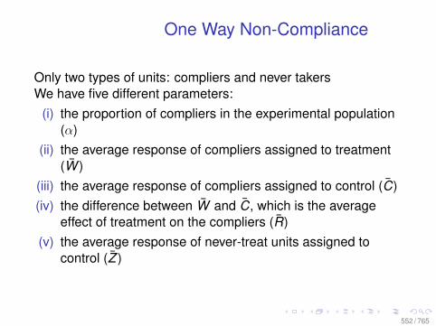
One Way Non-Compliance
Only two types of units: compliers and never takersWe have five different parameters:
(i) the proportion of compliers in the experimental population(α)
(ii) the average response of compliers assigned to treatment(W )
(iii) the average response of compliers assigned to control (C)(iv) the difference between W and C, which is the average
effect of treatment on the compliers (R)(v) the average response of never-treat units assigned to
control (Z )
552 / 765
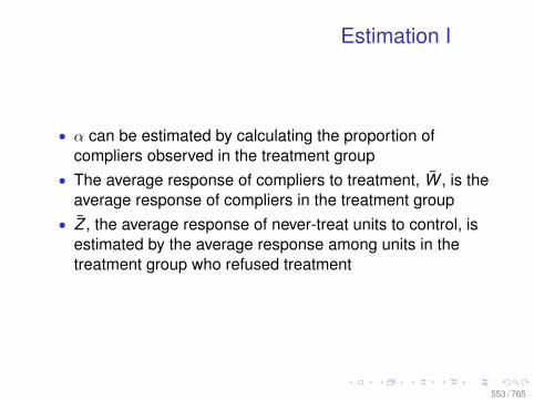
Estimation I
• α can be estimated by calculating the proportion ofcompliers observed in the treatment group
• The average response of compliers to treatment, W , is theaverage response of compliers in the treatment group
• Z , the average response of never-treat units to control, isestimated by the average response among units in thetreatment group who refused treatment
553 / 765
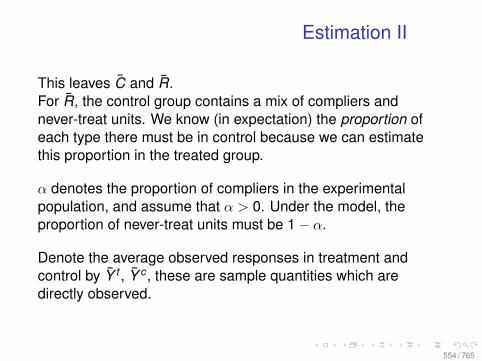
Estimation II
This leaves C and R.For R, the control group contains a mix of compliers andnever-treat units. We know (in expectation) the proportion ofeach type there must be in control because we can estimatethis proportion in the treated group.
α denotes the proportion of compliers in the experimentalpopulation, and assume that α > 0. Under the model, theproportion of never-treat units must be 1− α.
Denote the average observed responses in treatment andcontrol by Y t , Y c , these are sample quantities which aredirectly observed.
554 / 765
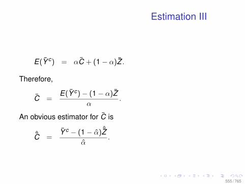
Estimation III
E(Y c) = αC + (1− α)Z .
Therefore,
C =E(Y c)− (1− α)Z
α.
An obvious estimator for C is
ˆC =Y c − (1− α) ˆZ
α.
555 / 765
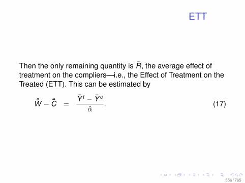
ETT
Then the only remaining quantity is R, the average effect oftreatment on the compliers—i.e., the Effect of Treatment on theTreated (ETT). This can be estimated by
ˆW − ˆC =Y t − Y c
α. (17)
556 / 765
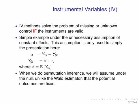
Instrumental Variables (IV)
• IV methods solve the problem of missing or unknowncontrol IF the instruments are valid
• Simple example under the unnecessary assumption ofconstant effects. This assumption is only used to simplythe presentation here:
α = Y1i − Y0i
Y0i = β + εi ,
where β ≡ E [Y0i ]
• When we do permutation inference, we will assume underthe null, unlike the Wald estimator, that the potentialoutcomes are fixed.
557 / 765
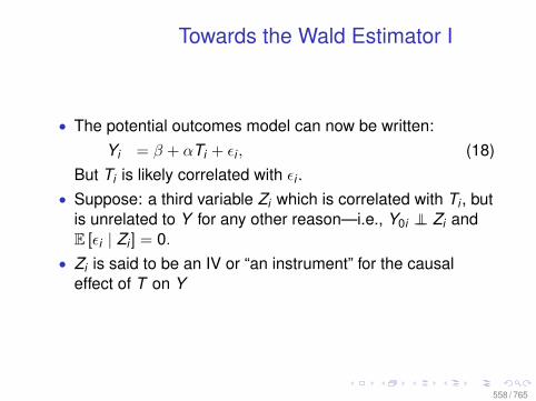
Towards the Wald Estimator I
• The potential outcomes model can now be written:Yi = β + αTi + εi , (18)
But Ti is likely correlated with εi .• Suppose: a third variable Zi which is correlated with Ti , but
is unrelated to Y for any other reason—i.e., Y0i ⊥⊥ Zi andE [εi | Zi ] = 0.
• Zi is said to be an IV or “an instrument” for the causaleffect of T on Y
558 / 765
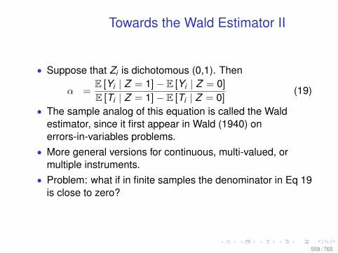
Towards the Wald Estimator II
• Suppose that Zi is dichotomous (0,1). Then
α =E [Yi | Z = 1]− E [Yi | Z = 0]
E [Ti | Z = 1]− E [Ti | Z = 0](19)
• The sample analog of this equation is called the Waldestimator, since it first appear in Wald (1940) onerrors-in-variables problems.
• More general versions for continuous, multi-valued, ormultiple instruments.
• Problem: what if in finite samples the denominator in Eq 19is close to zero?
559 / 765
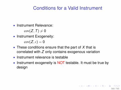
Conditions for a Valid Instrument
• Instrument Relevance:cov(Z ,T ) 6= 0
• Instrument Exogeneity:cov(Z , ε) = 0
• These conditions ensure that the part of X that iscorrelated with Z only contains exogenous variation
• Instrument relevance is testable• Instrument exogeneity is NOT testable. It must be true by
design
560 / 765
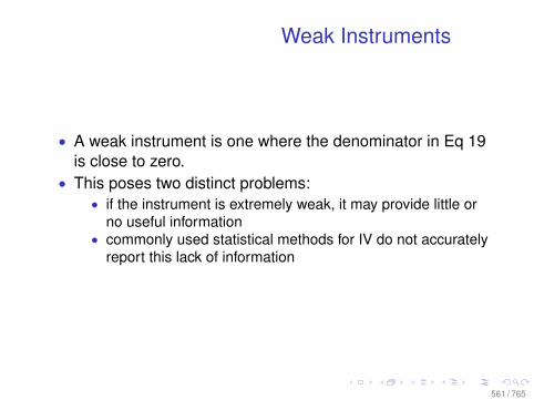
Weak Instruments
• A weak instrument is one where the denominator in Eq 19is close to zero.
• This poses two distinct problems:• if the instrument is extremely weak, it may provide little or
no useful information• commonly used statistical methods for IV do not accurately
report this lack of information
561 / 765
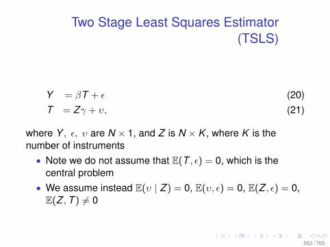
Two Stage Least Squares Estimator(TSLS)
Y = βT + ε (20)T = Zγ + υ, (21)
where Y , ε, υ are N × 1, and Z is N × K , where K is thenumber of instruments• Note we do not assume that E(T , ε) = 0, which is the
central problem• We assume instead E(υ | Z ) = 0, E(υ, ε) = 0, E(Z , ε) = 0,E(Z ,T ) 6= 0
562 / 765
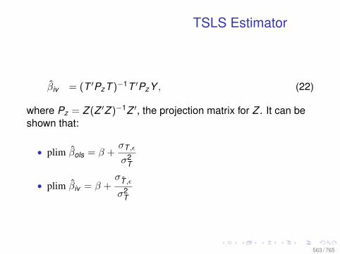
TSLS Estimator
βiv = (T ′PzT )−1T ′PzY , (22)
where Pz = Z (Z ′Z )−1Z ′, the projection matrix for Z . It can beshown that:
• plim βols = β +σT ,ε
σ2T
• plim βiv = β +σT ,ε
σ2T
563 / 765

Quarter of Birth and Returns toSchooling
• J. Angrist and Krueger (1991) want to estimate the causaleffect of education
• This is difficult, so they propose a way to estimate thecausal effect of compulsory school attendance on earnings
• Every state has a minimum number δ of years of schoolingthat all students must have
• But, the laws are written in terms of the age at which astudent can leave school
• Because birth dates vary, individual students are requiredto attend between δ and δ + 1 years of schooling
564 / 765
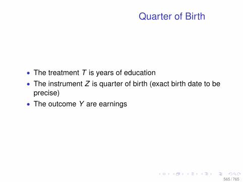
Quarter of Birth
• The treatment T is years of education• The instrument Z is quarter of birth (exact birth date to be
precise)• The outcome Y are earnings
565 / 765
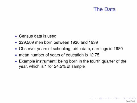
The Data
• Census data is used• 329,509 men born between 1930 and 1939• Observe: years of schooling, birth date, earnings in 1980• mean number of years of education is 12.75• Example instrument: being born in the fourth quarter of the
year, which is 1 for 24.5% of sample
566 / 765
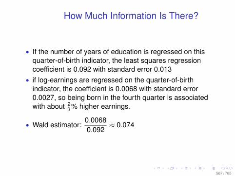
How Much Information Is There?
• If the number of years of education is regressed on thisquarter-of-birth indicator, the least squares regressioncoefficient is 0.092 with standard error 0.013
• if log-earnings are regressed on the quarter-of-birthindicator, the coefficient is 0.0068 with standard error0.0027, so being born in the fourth quarter is associatedwith about 2
3% higher earnings.
• Wald estimator:0.00680.092
≈ 0.074
567 / 765
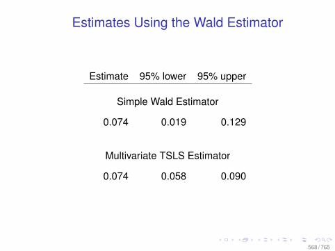
Estimates Using the Wald Estimator
Estimate 95% lower 95% upper
Simple Wald Estimator
0.074 0.019 0.129
Multivariate TSLS Estimator
0.074 0.058 0.090
568 / 765
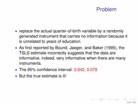
Problem
• replace the actual quarter-of-birth variable by a randomlygenerated instrument that carries no information because itis unrelated to years of education.
• As first reported by Bound, Jaeger, and Baker (1995), theTSLS estimate incorrectly suggests that the data areinformative, indeed, very informative when there are manyinstruments.
• The 95% confidence interval: 0.042, 0.078• But the true estimate is 0!
569 / 765
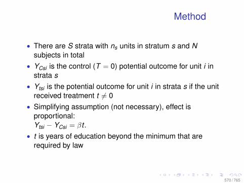
Method
• There are S strata with ns units in stratum s and Nsubjects in total
• YCsi is the control (T = 0) potential outcome for unit i instrata s
• Ytsi is the potential outcome for unit i in strata s if the unitreceived treatment t 6= 0
• Simplifying assumption (not necessary), effect isproportional:Ytsi − YCsi = βt .
• t is years of education beyond the minimum that arerequired by law
570 / 765
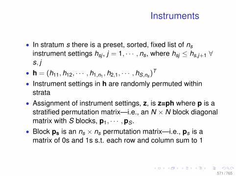
Instruments
• In stratum s there is a preset, sorted, fixed list of nsinstrument settings hsj , j = 1, · · · ,ns, where hsj ≤ hs,j+1 ∀s, j
• h = (h11,h12, · · · ,h1,n1 ,h2,1, · · · ,hS,ns )T
• Instrument settings in h are randomly permuted withinstrata
• Assignment of instrument settings, z, is z=ph where p is astratified permutation matrix—i.e., an N × N block diagonalmatrix with S blocks, p1, · · · ,pS.
• Block ps is an ns × ns permutation matrix—i.e., ps is amatrix of 0s and 1s s.t. each row and column sum to 1
571 / 765
Permutations
• Let Ω be the set of all stratified permutation matrices p, soΩ is a set containing |Ω| =
∏Ss=1 ns! matrices, where |Ω|
denotes the number of elements of the set Ω
• Pick a random P from Ω where Pr(P = p) =1|Ω| for each
p ∈ Ω
• Then Z = Ph is a random permutation of h within strata, sothe i th unit in stratum s receives instrument setting Zsi
572 / 765
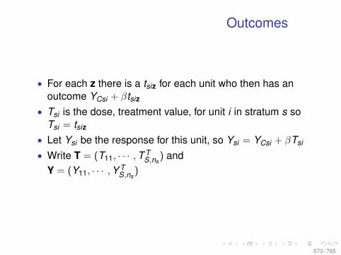
Outcomes
• For each z there is a tsiz for each unit who then has anoutcome YCsi + βtsiz
• Tsi is the dose, treatment value, for unit i in stratum s soTsi = tsiz
• Let Ysi be the response for this unit, so Ysi = YCsi + βTsi
• Write T = (T11, · · · ,T TS,ns
) andY = (Y11, · · · ,Y T
S,ns)
573 / 765
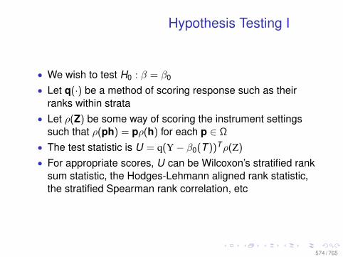
Hypothesis Testing I
• We wish to test H0 : β = β0
• Let q(·) be a method of scoring response such as theirranks within strata
• Let ρ(Z) be some way of scoring the instrument settingssuch that ρ(ph) = pρ(h) for each p ∈ Ω
• The test statistic is U = q(Y− β0(T ))Tρ(Z)
• For appropriate scores, U can be Wilcoxon’s stratified ranksum statistic, the Hodges-Lehmann aligned rank statistic,the stratified Spearman rank correlation, etc
574 / 765
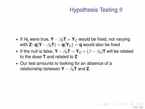
Hypothesis Testing II
• If H0 were true, Y− β0T = YC would be fixed, not varyingwith Z: q(Y− β0T) = q(YC) = q would also be fixed
• If the null is false, Y− β0T = YC + (β − β0)T will be relatedto the dose T and related to Z
• Our test amounts to looking for an absence of arelationship between Y− β0T and Z.
575 / 765
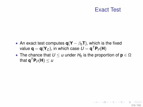
Exact Test
• An exact test computes q(Y− β0T), which is the fixedvalue q = q(YC), in which case U = qT Pρ(H)
• The chance that U ≤ u under H0 is the proportion of p ∈ Ωthat qT Pρ(H) ≤ u
576 / 765
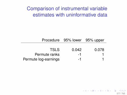
Comparison of instrumental variableestimates with uninformative data
Procedure 95% lower 95% upper
TSLS 0.042 0.078Permute ranks -1 1
Permute log-earnings -1 1
577 / 765
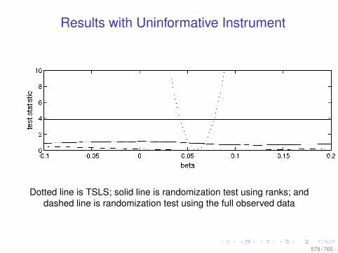
Results with Uninformative Instrument
Dotted line is TSLS; solid line is randomization test using ranks; anddashed line is randomization test using the full observed data
578 / 765

References
This treatment is based on:• G. W. Imbens and P. Rosenbaum (2005): “Robust,
Accurate Confidence Intervals with a Weak Instrument:Quarter of Birth and Education,” Journal of the RoyalStatistical Society, Series A, vol 168(1), 109–126.
• J. Angrist and Krueger (1991): “Does compulsory schoolattendance affect earnings?” QJE 1991; 106: 979–1019.
• Bound, Jaeger, and Baker (1995): “Problems withInstrumental Variables Estimation when the CorrelationBetween the Instruments and the Endogenous Regressorsis Weak,” JASA 90, June 1995, 443–450.
579 / 765

Background Reading
• Angrist, J.D. & Krueger, A.B. 2001. Instrumental Variablesand the Search for Identification: From Supply andDemand to Natural Experiments. Journal of EconomicPerspectives, 15(4), 69-85.
580 / 765
Example: Incumbency Advantage
• The purpose is to show that different identificationstrategies lead to different estimands.
• These differences are often subtle• Some research designs are so flawed, that even random
assignment would not identify the treatment effect ofinterest
• For details, see: Sekhon and Titiunik “Redistricting and thePersonal Vote: When Natural Experiments are NeitherNatural nor Experiments” http://sekhon.berkeley.edu/papers/incumb.pdf
581 / 765

Incumbency Advantage (IA)
• Extensive literature on the Incumbency Advantage (IA) inthe U.S.
• One of the most studied topics in political science• Senior scholars e.g.:
Ansolabehere, Brady, Cain, Cox, Erikson, Ferejohn,Fiorina, Gelman, Jacobson, Nagler, Katz, Kernell, King,Levitt, Mayhew, Niemi, Snyder, Stewart
• Junior/junior senior scholars e.g.:Ashworth, Bueno de Mesquita, Carson, Desposato,Engstrom, Gordon, Huber, Hirano, Landa, Lee, Prior,Roberts
582 / 765
Incumbency Advantage (IA)
• Extensive literature on the Incumbency Advantage (IA) inthe U.S.
• One of the most studied topics in political science• Senior scholars e.g.:
Ansolabehere, Brady, Cain, Cox, Erikson, Ferejohn,Fiorina, Gelman, Jacobson, Nagler, Katz, Kernell, King,Levitt, Mayhew, Niemi, Snyder, Stewart
• Junior/junior senior scholars e.g.:Ashworth, Bueno de Mesquita, Carson, Desposato,Engstrom, Gordon, Huber, Hirano, Landa, Lee, Prior,Roberts
583 / 765
So much work
“I am convinced that one more article demonstratingthat House incumbents tend to win reelection willinduce a spontaneous primal scream among allcongressional scholars across the nation.”Charles O. Jones (1981)
A Cautionary Tale. This should be an easy problem: clearquestion, a lot of data, and what people thought was a cleanidentification strategy.
584 / 765
So much work
“I am convinced that one more article demonstratingthat House incumbents tend to win reelection willinduce a spontaneous primal scream among allcongressional scholars across the nation.”Charles O. Jones (1981)
A Cautionary Tale. This should be an easy problem: clearquestion, a lot of data, and what people thought was a cleanidentification strategy.
585 / 765
So much work
“I am convinced that one more article demonstratingthat House incumbents tend to win reelection willinduce a spontaneous primal scream among allcongressional scholars across the nation.”Charles O. Jones (1981)
A Cautionary Tale. This should be an easy problem: clearquestion, a lot of data, and what people thought was a cleanidentification strategy.
586 / 765
Incumbency Advantage (IA)
• The Personal Incumbency Advantage is the candidatespecific advantage that results from the benefits of officeholding—e.g:• name recognition• constituency service• public position taking• providing pork
• Different from the Incumbent Party Advantage:• marginally, voters have a preference for remaining with the
same party they had before (D. S. Lee, 2008b)• parties have organizational advantages in some districts
587 / 765
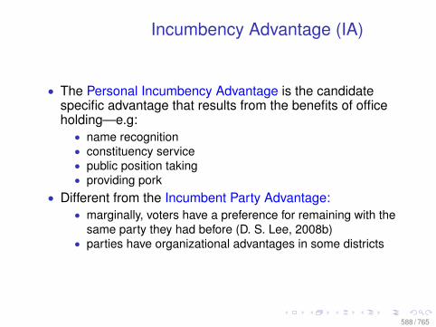
Incumbency Advantage (IA)
• The Personal Incumbency Advantage is the candidatespecific advantage that results from the benefits of officeholding—e.g:• name recognition• constituency service• public position taking• providing pork
• Different from the Incumbent Party Advantage:• marginally, voters have a preference for remaining with the
same party they had before (D. S. Lee, 2008b)• parties have organizational advantages in some districts
588 / 765
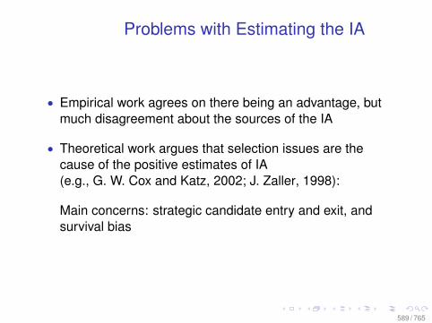
Problems with Estimating the IA
• Empirical work agrees on there being an advantage, butmuch disagreement about the sources of the IA
• Theoretical work argues that selection issues are thecause of the positive estimates of IA(e.g., G. W. Cox and Katz, 2002; J. Zaller, 1998):
Main concerns: strategic candidate entry and exit, andsurvival bias
589 / 765
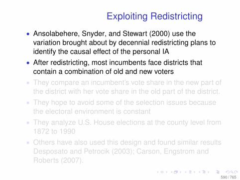
Exploiting Redistricting
• Ansolabehere, Snyder, and Stewart (2000) use thevariation brought about by decennial redistricting plans toidentify the causal effect of the personal IA
• After redistricting, most incumbents face districts thatcontain a combination of old and new voters
• They compare an incumbent’s vote share in the new part ofthe district with her vote share in the old part of the district.
• They hope to avoid some of the selection issues becausethe electoral environment is constant
• They analyze U.S. House elections at the county level from1872 to 1990
• Others have also used this design and found similar resultsDesposato and Petrocik (2003); Carson, Engstrom andRoberts (2007).
590 / 765
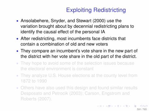
Exploiting Redistricting
• Ansolabehere, Snyder, and Stewart (2000) use thevariation brought about by decennial redistricting plans toidentify the causal effect of the personal IA
• After redistricting, most incumbents face districts thatcontain a combination of old and new voters
• They compare an incumbent’s vote share in the new part ofthe district with her vote share in the old part of the district.
• They hope to avoid some of the selection issues becausethe electoral environment is constant
• They analyze U.S. House elections at the county level from1872 to 1990
• Others have also used this design and found similar resultsDesposato and Petrocik (2003); Carson, Engstrom andRoberts (2007).
591 / 765
Exploiting Redistricting
• Ansolabehere, Snyder, and Stewart (2000) use thevariation brought about by decennial redistricting plans toidentify the causal effect of the personal IA
• After redistricting, most incumbents face districts thatcontain a combination of old and new voters
• They compare an incumbent’s vote share in the new part ofthe district with her vote share in the old part of the district.
• They hope to avoid some of the selection issues becausethe electoral environment is constant
• They analyze U.S. House elections at the county level from1872 to 1990
• Others have also used this design and found similar resultsDesposato and Petrocik (2003); Carson, Engstrom andRoberts (2007).
592 / 765
Exploiting Redistricting
• Ansolabehere, Snyder, and Stewart (2000) use thevariation brought about by decennial redistricting plans toidentify the causal effect of the personal IA
• After redistricting, most incumbents face districts thatcontain a combination of old and new voters
• They compare an incumbent’s vote share in the new part ofthe district with her vote share in the old part of the district.
• They hope to avoid some of the selection issues becausethe electoral environment is constant
• They analyze U.S. House elections at the county level from1872 to 1990
• Others have also used this design and found similar resultsDesposato and Petrocik (2003); Carson, Engstrom andRoberts (2007).
593 / 765
Using Redistricting to EstimateIncumbency
• We propose a new method for estimating incumbencyadvantage (IA)
• Previous redistricting designs result in biased estimates ofincumbency
• The wrong potential outcomes were used• Leads to bias even if voters were redistricted randomly!• In practice, a selection on observables assumption must
be made• The selection on observables assumption in prior work is
theoretically implausible and fails a placebo test• Use redistricting to answer other questions as well—e.g.,
how voters respond to candidates’ race and ethnicity
594 / 765
Using Redistricting to EstimateIncumbency
• We propose a new method for estimating incumbencyadvantage (IA)
• Previous redistricting designs result in biased estimates ofincumbency
• The wrong potential outcomes were used• Leads to bias even if voters were redistricted randomly!• In practice, a selection on observables assumption must
be made• The selection on observables assumption in prior work is
theoretically implausible and fails a placebo test• Use redistricting to answer other questions as well—e.g.,
how voters respond to candidates’ race and ethnicity
595 / 765
Using Redistricting to EstimateIncumbency
• We propose a new method for estimating incumbencyadvantage (IA)
• Previous redistricting designs result in biased estimates ofincumbency
• The wrong potential outcomes were used• Leads to bias even if voters were redistricted randomly!• In practice, a selection on observables assumption must
be made• The selection on observables assumption in prior work is
theoretically implausible and fails a placebo test• Use redistricting to answer other questions as well—e.g.,
how voters respond to candidates’ race and ethnicity
596 / 765
Using Redistricting to EstimateIncumbency
• We propose a new method for estimating incumbencyadvantage (IA)
• Previous redistricting designs result in biased estimates ofincumbency
• The wrong potential outcomes were used• Leads to bias even if voters were redistricted randomly!• In practice, a selection on observables assumption must
be made• The selection on observables assumption in prior work is
theoretically implausible and fails a placebo test• Use redistricting to answer other questions as well—e.g.,
how voters respond to candidates’ race and ethnicity
597 / 765
Where we are Going
One interpretation of our results:• No (TX) or little (CA) personal incumbency advantage in
U.S. House elections• Significant and large incumbent party effects
Results are more consistent with:• Voters learn the type of new incumbent very quickly• Unless there is a mismatch between the partisanship of
voters and their incumbent. Then, voters take more time tolearn the type of their incumbent
598 / 765
Where we are Going
One interpretation of our results:• No (TX) or little (CA) personal incumbency advantage in
U.S. House elections• Significant and large incumbent party effects
Results are more consistent with:• Voters learn the type of new incumbent very quickly• Unless there is a mismatch between the partisanship of
voters and their incumbent. Then, voters take more time tolearn the type of their incumbent
599 / 765
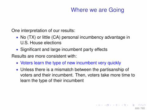
Where we are Going
One interpretation of our results:• No (TX) or little (CA) personal incumbency advantage in
U.S. House elections• Significant and large incumbent party effects
Results are more consistent with:• Voters learn the type of new incumbent very quickly• Unless there is a mismatch between the partisanship of
voters and their incumbent. Then, voters take more time tolearn the type of their incumbent
600 / 765
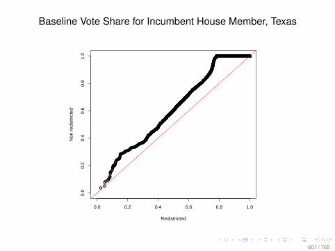
Baseline Vote Share for Incumbent House Member, Texas
0.0 0.2 0.4 0.6 0.8 1.0
0.0
0.2
0.4
0.6
0.8
1.0
Redistricted
Non
red
istr
icte
d
601 / 765
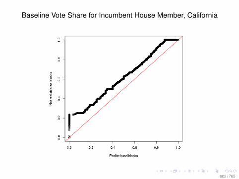
Baseline Vote Share for Incumbent House Member, California
602 / 765

Lagged Democratic Win in RDD: 1st and 2nd-order polynomial
603 / 765

Lagged Democratic Win in RDD: 3rd and 4th-order polynomial
604 / 765

Lagged Democratic Win in RDD: 8th-order polynomial
605 / 765
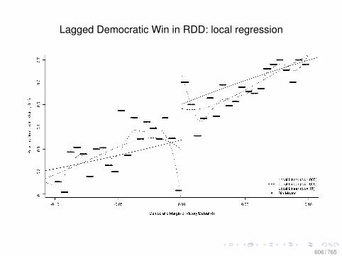
Lagged Democratic Win in RDD: local regression
606 / 765
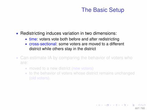
The Basic Setup
• Redistricting induces variation in two dimensions:• time: voters vote both before and after redistricting• cross-sectional: some voters are moved to a different
district while others stay in the district
• Can estimate IA by comparing the behavior of voters whoare:• moved to a new district (new voters)• to the behavior of voters whose district remains unchanged
(old voters).
607 / 765
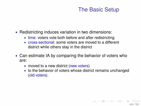
The Basic Setup
• Redistricting induces variation in two dimensions:• time: voters vote both before and after redistricting• cross-sectional: some voters are moved to a different
district while others stay in the district
• Can estimate IA by comparing the behavior of voters whoare:• moved to a new district (new voters)• to the behavior of voters whose district remains unchanged
(old voters).
608 / 765
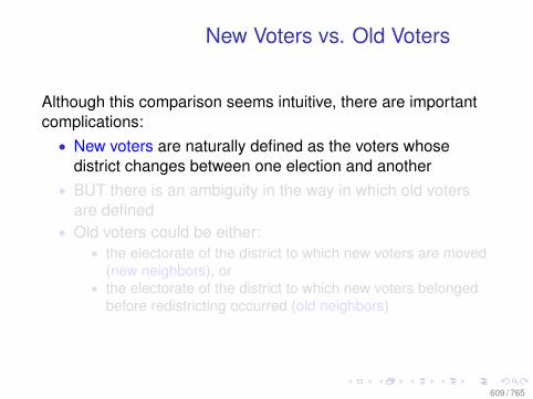
New Voters vs. Old Voters
Although this comparison seems intuitive, there are importantcomplications:• New voters are naturally defined as the voters whose
district changes between one election and another• BUT there is an ambiguity in the way in which old voters
are defined• Old voters could be either:
• the electorate of the district to which new voters are moved(new neighbors), or
• the electorate of the district to which new voters belongedbefore redistricting occurred (old neighbors)
609 / 765
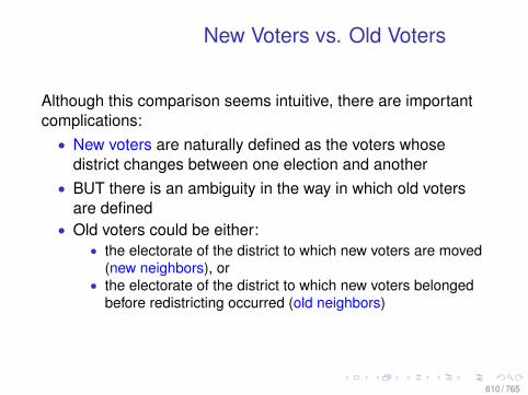
New Voters vs. Old Voters
Although this comparison seems intuitive, there are importantcomplications:• New voters are naturally defined as the voters whose
district changes between one election and another• BUT there is an ambiguity in the way in which old voters
are defined• Old voters could be either:
• the electorate of the district to which new voters are moved(new neighbors), or
• the electorate of the district to which new voters belongedbefore redistricting occurred (old neighbors)
610 / 765
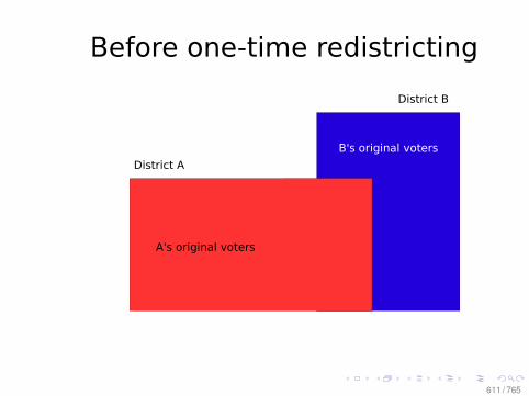
Before one-time redistricting
District A
District B
B's original voters
A's original voters
611 / 765
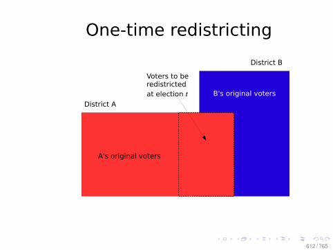
One-time redistricting
District A
District B
Voters to be redistricted
at election t B's original voters
A's original voters
612 / 765
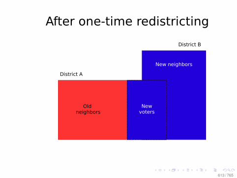
After one-time redistricting
District A
District B
Old neighbors
New voters
New neighbors
613 / 765
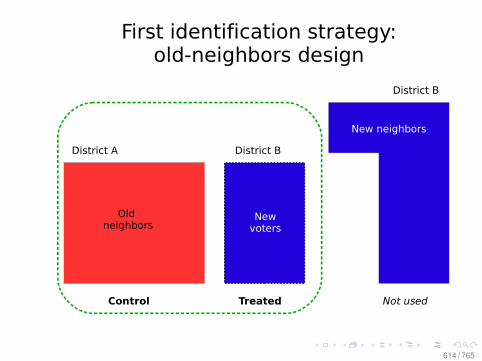
First identification strategy:old-neighbors design
District B
New neighbors
Not used
District A
Control Treated
District B
New voters
Old neighbors
614 / 765
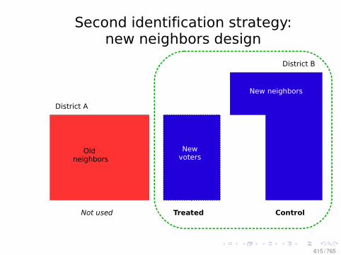
Second identification strategy:new neighbors design
District B
New neighbors
Control
District A
Not used Treated
New voters
Old neighbors
615 / 765
Two Obvious Designs
There are then two obvious designs under the randomizationwhere everyone is in a certain district at t − 1 and someprecincts are randomly moved to another district at t .• Compare new voters with old neighbors• Compare new voters with new neighbors—this is the
Ansolabehere, Snyder, and Stewart (2000) design• Randomization ensures exchangeability for the first design,
but not the second• This occurs because the history of new voters with new
neighbors is not balanced by randomization
616 / 765
Two Obvious Designs
There are then two obvious designs under the randomizationwhere everyone is in a certain district at t − 1 and someprecincts are randomly moved to another district at t .• Compare new voters with old neighbors• Compare new voters with new neighbors—this is the
Ansolabehere, Snyder, and Stewart (2000) design• Randomization ensures exchangeability for the first design,
but not the second• This occurs because the history of new voters with new
neighbors is not balanced by randomization
617 / 765
Two Obvious Designs
There are then two obvious designs under the randomizationwhere everyone is in a certain district at t − 1 and someprecincts are randomly moved to another district at t .• Compare new voters with old neighbors• Compare new voters with new neighbors—this is the
Ansolabehere, Snyder, and Stewart (2000) design• Randomization ensures exchangeability for the first design,
but not the second• This occurs because the history of new voters with new
neighbors is not balanced by randomization
618 / 765
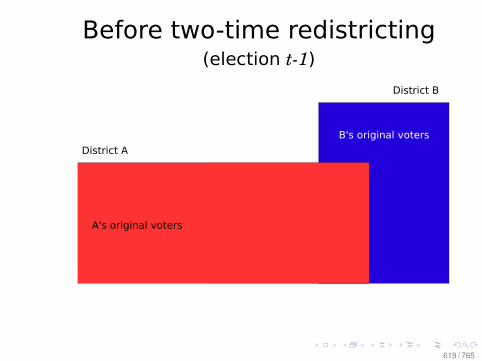
Before two-time redistricting(election t-1)
District A
District B
B's original voters
A's original voters
619 / 765
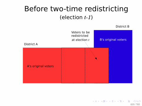
District A
District B
Voters to be redistricted
at election t B's original voters
A's original voters
Before two-time redistricting(election t-1)
620 / 765
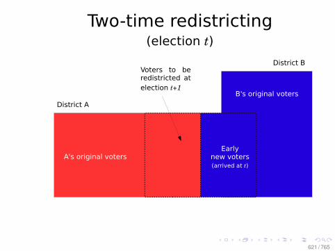
Two-time redistricting(election t)
District A
District B
B's original voters
A's original votersEarly
new voters
(arrived at t)
Voters to be redistricted at
election t+1
621 / 765
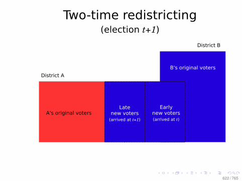
Two-time redistricting(election t+1)
District A
District B
Earlynew voters
(arrived at t)
B's original voters
A's original votersLate
new voters
(arrived at t+1)
622 / 765
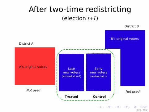
After two-time redistricting(election t+1)
District A
District B
Earlynew voters
(arrived at t)
B's original voters
A's original votersLate
new voters
(arrived at t+1)
Control
Not used
Treated
Not used
623 / 765
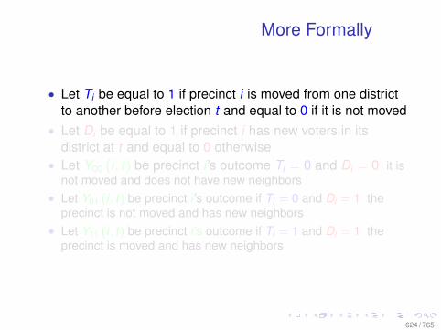
More Formally
• Let Ti be equal to 1 if precinct i is moved from one districtto another before election t and equal to 0 if it is not moved
• Let Di be equal to 1 if precinct i has new voters in itsdistrict at t and equal to 0 otherwise
• Let Y00 (i , t) be precinct i ’s outcome Ti = 0 and Di = 0 it isnot moved and does not have new neighbors
• Let Y01 (i , t) be precinct i ’s outcome if Ti = 0 and Di = 1 theprecinct is not moved and has new neighbors
• Let Y11 (i , t) be precinct i ’s outcome if Ti = 1 and Di = 1 theprecinct is moved and has new neighbors
624 / 765
More Formally
• Let Ti be equal to 1 if precinct i is moved from one districtto another before election t and equal to 0 if it is not moved
• Let Di be equal to 1 if precinct i has new voters in itsdistrict at t and equal to 0 otherwise
• Let Y00 (i , t) be precinct i ’s outcome Ti = 0 and Di = 0 it isnot moved and does not have new neighbors
• Let Y01 (i , t) be precinct i ’s outcome if Ti = 0 and Di = 1 theprecinct is not moved and has new neighbors
• Let Y11 (i , t) be precinct i ’s outcome if Ti = 1 and Di = 1 theprecinct is moved and has new neighbors
625 / 765
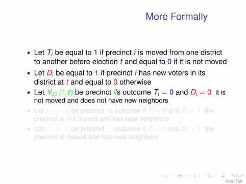
More Formally
• Let Ti be equal to 1 if precinct i is moved from one districtto another before election t and equal to 0 if it is not moved
• Let Di be equal to 1 if precinct i has new voters in itsdistrict at t and equal to 0 otherwise
• Let Y00 (i , t) be precinct i ’s outcome Ti = 0 and Di = 0 it isnot moved and does not have new neighbors
• Let Y01 (i , t) be precinct i ’s outcome if Ti = 0 and Di = 1 theprecinct is not moved and has new neighbors
• Let Y11 (i , t) be precinct i ’s outcome if Ti = 1 and Di = 1 theprecinct is moved and has new neighbors
626 / 765
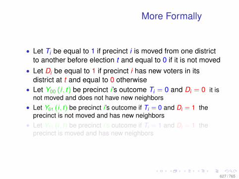
More Formally
• Let Ti be equal to 1 if precinct i is moved from one districtto another before election t and equal to 0 if it is not moved
• Let Di be equal to 1 if precinct i has new voters in itsdistrict at t and equal to 0 otherwise
• Let Y00 (i , t) be precinct i ’s outcome Ti = 0 and Di = 0 it isnot moved and does not have new neighbors
• Let Y01 (i , t) be precinct i ’s outcome if Ti = 0 and Di = 1 theprecinct is not moved and has new neighbors
• Let Y11 (i , t) be precinct i ’s outcome if Ti = 1 and Di = 1 theprecinct is moved and has new neighbors
627 / 765
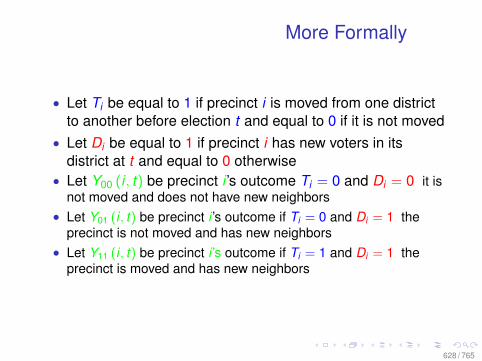
More Formally
• Let Ti be equal to 1 if precinct i is moved from one districtto another before election t and equal to 0 if it is not moved
• Let Di be equal to 1 if precinct i has new voters in itsdistrict at t and equal to 0 otherwise
• Let Y00 (i , t) be precinct i ’s outcome Ti = 0 and Di = 0 it isnot moved and does not have new neighbors
• Let Y01 (i , t) be precinct i ’s outcome if Ti = 0 and Di = 1 theprecinct is not moved and has new neighbors
• Let Y11 (i , t) be precinct i ’s outcome if Ti = 1 and Di = 1 theprecinct is moved and has new neighbors
628 / 765
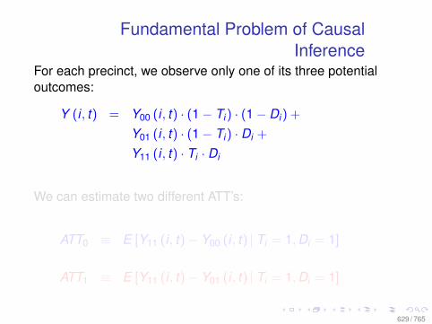
Fundamental Problem of CausalInference
For each precinct, we observe only one of its three potentialoutcomes:
Y (i , t) = Y00 (i , t) · (1− Ti) · (1− Di) +
Y01 (i , t) · (1− Ti) · Di +
Y11 (i , t) · Ti · Di
We can estimate two different ATT’s:
ATT0 ≡ E [Y11 (i , t)− Y00 (i , t) | Ti = 1,Di = 1]
ATT1 ≡ E [Y11 (i , t)− Y01 (i , t) | Ti = 1,Di = 1]
629 / 765
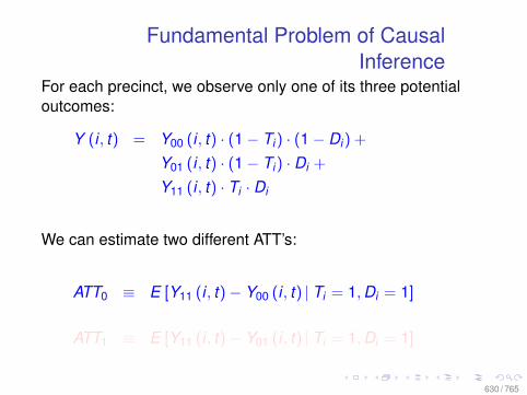
Fundamental Problem of CausalInference
For each precinct, we observe only one of its three potentialoutcomes:
Y (i , t) = Y00 (i , t) · (1− Ti) · (1− Di) +
Y01 (i , t) · (1− Ti) · Di +
Y11 (i , t) · Ti · Di
We can estimate two different ATT’s:
ATT0 ≡ E [Y11 (i , t)− Y00 (i , t) | Ti = 1,Di = 1]
ATT1 ≡ E [Y11 (i , t)− Y01 (i , t) | Ti = 1,Di = 1]
630 / 765
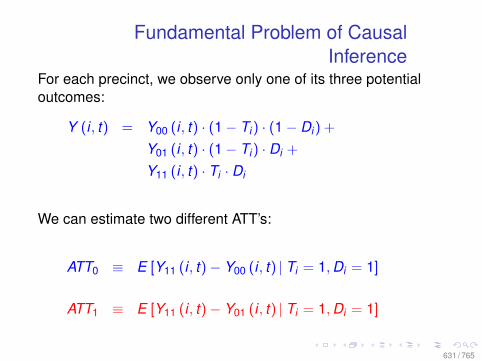
Fundamental Problem of CausalInference
For each precinct, we observe only one of its three potentialoutcomes:
Y (i , t) = Y00 (i , t) · (1− Ti) · (1− Di) +
Y01 (i , t) · (1− Ti) · Di +
Y11 (i , t) · Ti · Di
We can estimate two different ATT’s:
ATT0 ≡ E [Y11 (i , t)− Y00 (i , t) | Ti = 1,Di = 1]
ATT1 ≡ E [Y11 (i , t)− Y01 (i , t) | Ti = 1,Di = 1]
631 / 765
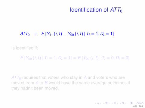
Identification of ATT0
ATT0 ≡ E [Y11 (i , t)− Y00 (i , t) | Ti = 1,Di = 1]
Is identified if:
E [Y00 (i , t) | Ti = 1,Di = 1] = E [Y00 (i , t) | Ti = 0,Di = 0]
ATT0 requires that voters who stay in A and voters who aremoved from A to B would have the same average outcomes ifthey hadn’t been moved.
632 / 765
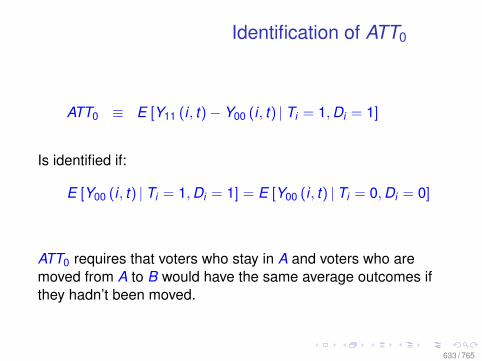
Identification of ATT0
ATT0 ≡ E [Y11 (i , t)− Y00 (i , t) | Ti = 1,Di = 1]
Is identified if:
E [Y00 (i , t) | Ti = 1,Di = 1] = E [Y00 (i , t) | Ti = 0,Di = 0]
ATT0 requires that voters who stay in A and voters who aremoved from A to B would have the same average outcomes ifthey hadn’t been moved.
633 / 765
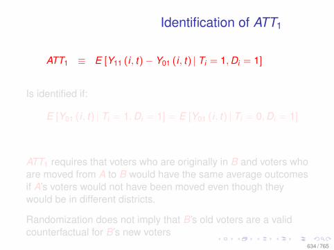
Identification of ATT1
ATT1 ≡ E [Y11 (i , t)− Y01 (i , t) | Ti = 1,Di = 1]
Is identified if:
E [Y01 (i , t) | Ti = 1,Di = 1] = E [Y01 (i , t) | Ti = 0,Di = 1]
ATT1 requires that voters who are originally in B and voters whoare moved from A to B would have the same average outcomesif A’s voters would not have been moved even though theywould be in different districts.
Randomization does not imply that B’s old voters are a validcounterfactual for B’s new voters
634 / 765
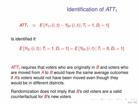
Identification of ATT1
ATT1 ≡ E [Y11 (i , t)− Y01 (i , t) | Ti = 1,Di = 1]
Is identified if:
E [Y01 (i , t) | Ti = 1,Di = 1] = E [Y01 (i , t) | Ti = 0,Di = 1]
ATT1 requires that voters who are originally in B and voters whoare moved from A to B would have the same average outcomesif A’s voters would not have been moved even though theywould be in different districts.
Randomization does not imply that B’s old voters are a validcounterfactual for B’s new voters
635 / 765
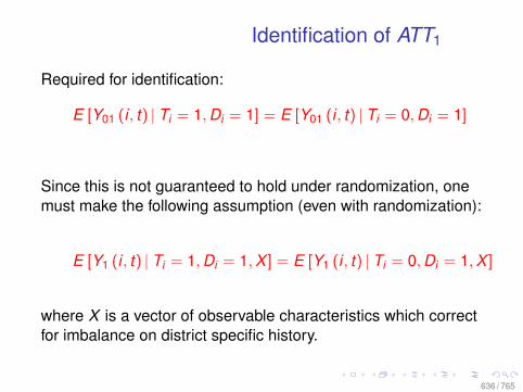
Identification of ATT1
Required for identification:
E [Y01 (i , t) | Ti = 1,Di = 1] = E [Y01 (i , t) | Ti = 0,Di = 1]
Since this is not guaranteed to hold under randomization, onemust make the following assumption (even with randomization):
E [Y1 (i , t) | Ti = 1,Di = 1,X ] = E [Y1 (i , t) | Ti = 0,Di = 1,X ]
where X is a vector of observable characteristics which correctfor imbalance on district specific history.
636 / 765
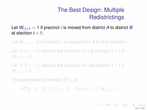
The Best Design: MultipleRedistrictings
Let Wi,t+1 = 1 if precinct i is moved from district A to district Bat election t + 1.
Let Wi,t+1 = 0 if precinct i is moved from A to B at election t .
Let Y0 (i , t + 1) denote the outcome of i at election t + 1 ifWi,t+1 = 0
Let Y1 (i , t + 1) denote the outcome of i at election t + 1 ifWi,t+1 = 1
The parameter of interest ATTB is
ATTB ≡ E[Y1 (i , t + 1)− Y0 (i , t + 1) |Wi,t+1 = 1
]
637 / 765
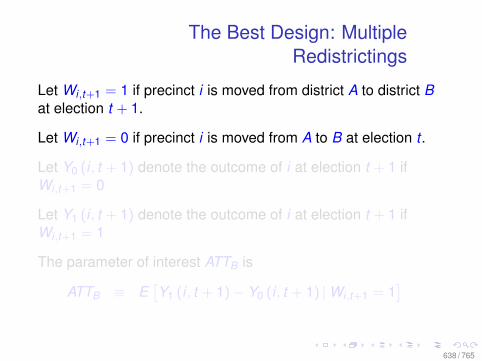
The Best Design: MultipleRedistrictings
Let Wi,t+1 = 1 if precinct i is moved from district A to district Bat election t + 1.
Let Wi,t+1 = 0 if precinct i is moved from A to B at election t .
Let Y0 (i , t + 1) denote the outcome of i at election t + 1 ifWi,t+1 = 0
Let Y1 (i , t + 1) denote the outcome of i at election t + 1 ifWi,t+1 = 1
The parameter of interest ATTB is
ATTB ≡ E[Y1 (i , t + 1)− Y0 (i , t + 1) |Wi,t+1 = 1
]
638 / 765
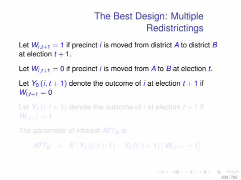
The Best Design: MultipleRedistrictings
Let Wi,t+1 = 1 if precinct i is moved from district A to district Bat election t + 1.
Let Wi,t+1 = 0 if precinct i is moved from A to B at election t .
Let Y0 (i , t + 1) denote the outcome of i at election t + 1 ifWi,t+1 = 0
Let Y1 (i , t + 1) denote the outcome of i at election t + 1 ifWi,t+1 = 1
The parameter of interest ATTB is
ATTB ≡ E[Y1 (i , t + 1)− Y0 (i , t + 1) |Wi,t+1 = 1
]
639 / 765
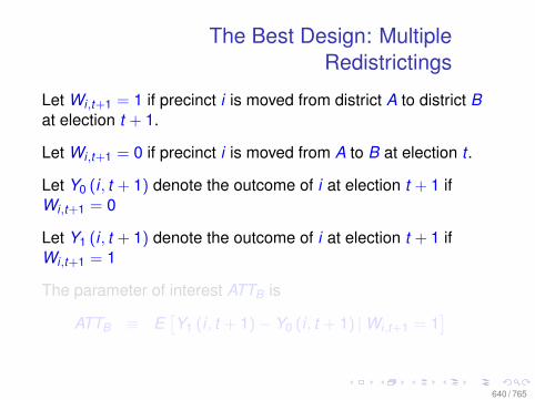
The Best Design: MultipleRedistrictings
Let Wi,t+1 = 1 if precinct i is moved from district A to district Bat election t + 1.
Let Wi,t+1 = 0 if precinct i is moved from A to B at election t .
Let Y0 (i , t + 1) denote the outcome of i at election t + 1 ifWi,t+1 = 0
Let Y1 (i , t + 1) denote the outcome of i at election t + 1 ifWi,t+1 = 1
The parameter of interest ATTB is
ATTB ≡ E[Y1 (i , t + 1)− Y0 (i , t + 1) |Wi,t+1 = 1
]
640 / 765
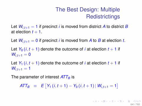
The Best Design: MultipleRedistrictings
Let Wi,t+1 = 1 if precinct i is moved from district A to district Bat election t + 1.
Let Wi,t+1 = 0 if precinct i is moved from A to B at election t .
Let Y0 (i , t + 1) denote the outcome of i at election t + 1 ifWi,t+1 = 0
Let Y1 (i , t + 1) denote the outcome of i at election t + 1 ifWi,t+1 = 1
The parameter of interest ATTB is
ATTB ≡ E[Y1 (i , t + 1)− Y0 (i , t + 1) |Wi,t+1 = 1
]
641 / 765
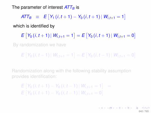
The parameter of interest ATTB is
ATTB ≡ E[Y1 (i , t + 1)− Y0 (i , t + 1) |Wi,t+1 = 1
]which is identified by
E[Y0 (i , t + 1) |Wi,t+1 = 1
]= E
[Y0 (i , t + 1) |Wi,t+1 = 0
]By randomization we have
E[Y0 (i , t − 1) |Wi,t+1 = 1
]= E
[Y0 (i , t − 1) |Wi,t+1 = 0
]Randomization along with the following stability assumptionprovides identification:
E[Y0 (i , t + 1)− Y0 (i , t − 1) |Wi,t+1 = 1
]=
E[Y0 (i , t + 1)− Y0 (i , t − 1) |Wi,t+1 = 0
]
642 / 765
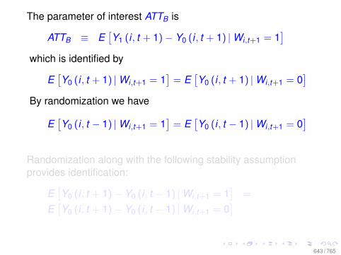
The parameter of interest ATTB is
ATTB ≡ E[Y1 (i , t + 1)− Y0 (i , t + 1) |Wi,t+1 = 1
]which is identified by
E[Y0 (i , t + 1) |Wi,t+1 = 1
]= E
[Y0 (i , t + 1) |Wi,t+1 = 0
]By randomization we have
E[Y0 (i , t − 1) |Wi,t+1 = 1
]= E
[Y0 (i , t − 1) |Wi,t+1 = 0
]Randomization along with the following stability assumptionprovides identification:
E[Y0 (i , t + 1)− Y0 (i , t − 1) |Wi,t+1 = 1
]=
E[Y0 (i , t + 1)− Y0 (i , t − 1) |Wi,t+1 = 0
]
643 / 765
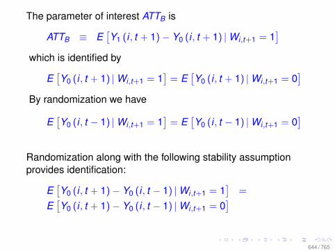
The parameter of interest ATTB is
ATTB ≡ E[Y1 (i , t + 1)− Y0 (i , t + 1) |Wi,t+1 = 1
]which is identified by
E[Y0 (i , t + 1) |Wi,t+1 = 1
]= E
[Y0 (i , t + 1) |Wi,t+1 = 0
]By randomization we have
E[Y0 (i , t − 1) |Wi,t+1 = 1
]= E
[Y0 (i , t − 1) |Wi,t+1 = 0
]Randomization along with the following stability assumptionprovides identification:
E[Y0 (i , t + 1)− Y0 (i , t − 1) |Wi,t+1 = 1
]=
E[Y0 (i , t + 1)− Y0 (i , t − 1) |Wi,t+1 = 0
]
644 / 765
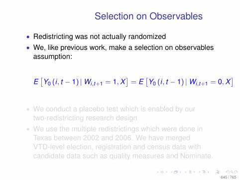
Selection on Observables
• Redistricting was not actually randomized• We, like previous work, make a selection on observables
assumption:
E[Y0 (i , t − 1) |Wi,t+1 = 1,X
]= E
[Y0 (i , t − 1) |Wi,t+1 = 0,X
]• We conduct a placebo test which is enabled by our
two-redistricting research design• We use the multiple redistrictings which were done in
Texas between 2002 and 2006. We have mergedVTD-level election, registration and census data withcandidate data such as quality measures and Nominate.
645 / 765
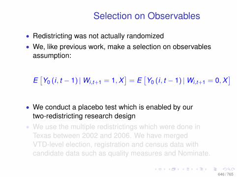
Selection on Observables
• Redistricting was not actually randomized• We, like previous work, make a selection on observables
assumption:
E[Y0 (i , t − 1) |Wi,t+1 = 1,X
]= E
[Y0 (i , t − 1) |Wi,t+1 = 0,X
]• We conduct a placebo test which is enabled by our
two-redistricting research design• We use the multiple redistrictings which were done in
Texas between 2002 and 2006. We have mergedVTD-level election, registration and census data withcandidate data such as quality measures and Nominate.
646 / 765
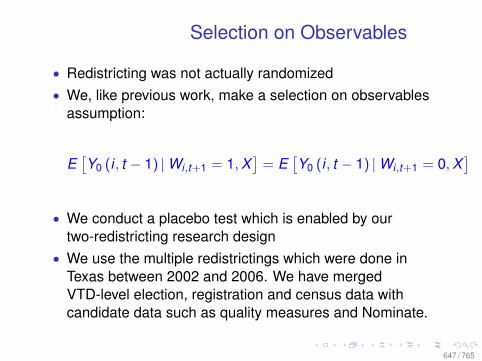
Selection on Observables
• Redistricting was not actually randomized• We, like previous work, make a selection on observables
assumption:
E[Y0 (i , t − 1) |Wi,t+1 = 1,X
]= E
[Y0 (i , t − 1) |Wi,t+1 = 0,X
]• We conduct a placebo test which is enabled by our
two-redistricting research design• We use the multiple redistrictings which were done in
Texas between 2002 and 2006. We have mergedVTD-level election, registration and census data withcandidate data such as quality measures and Nominate.
647 / 765
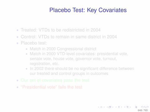
Placebo Test: Key Covariates
• Treated: VTDs to be redistricted in 2004• Control: VTDs to remain in same district in 2004• Placebo test:
• Match in 2000 Congressional district• Match in 2000 VTD-level covariates: presidential vote,
senate vote, house vote, governor vote, turnout,registration, etc.
• In 2002 there should be no significant difference betweenour treated and control groups in outcomes
• Our set of covariates pass the test• “Presidential vote” fails the test
648 / 765
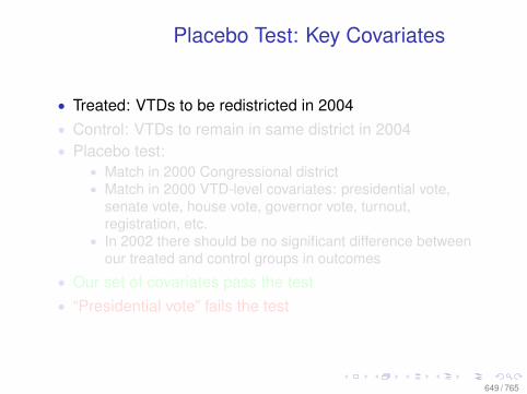
Placebo Test: Key Covariates
• Treated: VTDs to be redistricted in 2004• Control: VTDs to remain in same district in 2004• Placebo test:
• Match in 2000 Congressional district• Match in 2000 VTD-level covariates: presidential vote,
senate vote, house vote, governor vote, turnout,registration, etc.
• In 2002 there should be no significant difference betweenour treated and control groups in outcomes
• Our set of covariates pass the test• “Presidential vote” fails the test
649 / 765
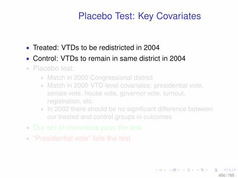
Placebo Test: Key Covariates
• Treated: VTDs to be redistricted in 2004• Control: VTDs to remain in same district in 2004• Placebo test:
• Match in 2000 Congressional district• Match in 2000 VTD-level covariates: presidential vote,
senate vote, house vote, governor vote, turnout,registration, etc.
• In 2002 there should be no significant difference betweenour treated and control groups in outcomes
• Our set of covariates pass the test• “Presidential vote” fails the test
650 / 765
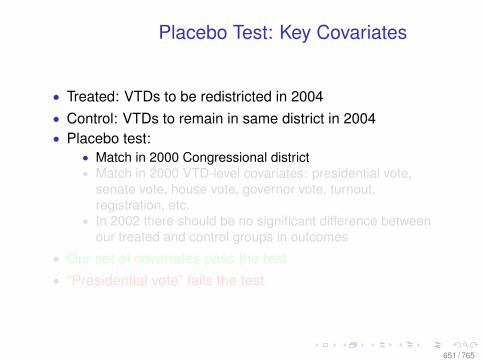
Placebo Test: Key Covariates
• Treated: VTDs to be redistricted in 2004• Control: VTDs to remain in same district in 2004• Placebo test:
• Match in 2000 Congressional district• Match in 2000 VTD-level covariates: presidential vote,
senate vote, house vote, governor vote, turnout,registration, etc.
• In 2002 there should be no significant difference betweenour treated and control groups in outcomes
• Our set of covariates pass the test• “Presidential vote” fails the test
651 / 765
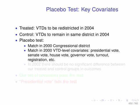
Placebo Test: Key Covariates
• Treated: VTDs to be redistricted in 2004• Control: VTDs to remain in same district in 2004• Placebo test:
• Match in 2000 Congressional district• Match in 2000 VTD-level covariates: presidential vote,
senate vote, house vote, governor vote, turnout,registration, etc.
• In 2002 there should be no significant difference betweenour treated and control groups in outcomes
• Our set of covariates pass the test• “Presidential vote” fails the test
652 / 765
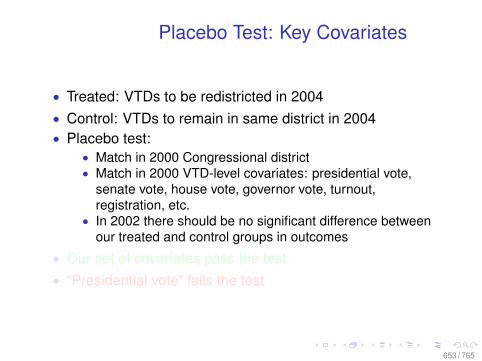
Placebo Test: Key Covariates
• Treated: VTDs to be redistricted in 2004• Control: VTDs to remain in same district in 2004• Placebo test:
• Match in 2000 Congressional district• Match in 2000 VTD-level covariates: presidential vote,
senate vote, house vote, governor vote, turnout,registration, etc.
• In 2002 there should be no significant difference betweenour treated and control groups in outcomes
• Our set of covariates pass the test• “Presidential vote” fails the test
653 / 765
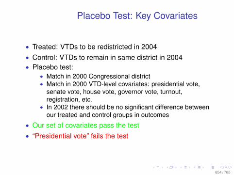
Placebo Test: Key Covariates
• Treated: VTDs to be redistricted in 2004• Control: VTDs to remain in same district in 2004• Placebo test:
• Match in 2000 Congressional district• Match in 2000 VTD-level covariates: presidential vote,
senate vote, house vote, governor vote, turnout,registration, etc.
• In 2002 there should be no significant difference betweenour treated and control groups in outcomes
• Our set of covariates pass the test• “Presidential vote” fails the test
654 / 765
Estimation
• Genetic Matching (GenMatch) is used to achieve covariatebalance
• Hodges-Lehmann interval estimation, bivariateoverdispersed GLM estimation and Abadie-Imbens CIs arecalculated post-matching. Substantive inferences remainunchanged.
• Hodges-Lehmann intervals are presented in the following.
655 / 765
Estimation
• Genetic Matching (GenMatch) is used to achieve covariatebalance
• Hodges-Lehmann interval estimation, bivariateoverdispersed GLM estimation and Abadie-Imbens CIs arecalculated post-matching. Substantive inferences remainunchanged.
• Hodges-Lehmann intervals are presented in the following.
656 / 765
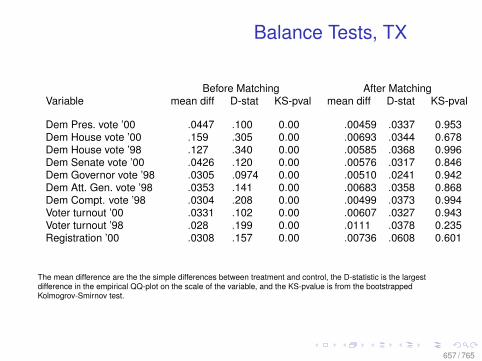
Balance Tests, TX
Before Matching After MatchingVariable mean diff D-stat KS-pval mean diff D-stat KS-pval
Dem Pres. vote ’00 .0447 .100 0.00 .00459 .0337 0.953Dem House vote ’00 .159 .305 0.00 .00693 .0344 0.678Dem House vote ’98 .127 .340 0.00 .00585 .0368 0.996Dem Senate vote ’00 .0426 .120 0.00 .00576 .0317 0.846Dem Governor vote ’98 .0305 .0974 0.00 .00510 .0241 0.942Dem Att. Gen. vote ’98 .0353 .141 0.00 .00683 .0358 0.868Dem Compt. vote ’98 .0304 .208 0.00 .00499 .0373 0.994Voter turnout ’00 .0331 .102 0.00 .00607 .0327 0.943Voter turnout ’98 .028 .199 0.00 .0111 .0378 0.235Registration ’00 .0308 .157 0.00 .00736 .0608 0.601
The mean difference are the the simple differences between treatment and control, the D-statistic is the largestdifference in the empirical QQ-plot on the scale of the variable, and the KS-pvalue is from the bootstrappedKolmogrov-Smirnov test.
657 / 765
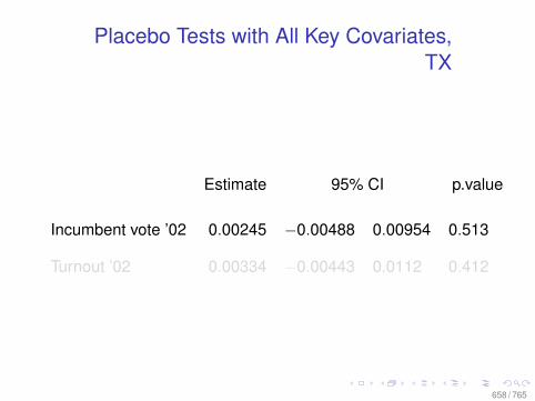
Placebo Tests with All Key Covariates,TX
Estimate 95% CI p.value
Incumbent vote ’02 0.00245 −0.00488 0.00954 0.513
Turnout ’02 0.00334 −0.00443 0.0112 0.412
658 / 765
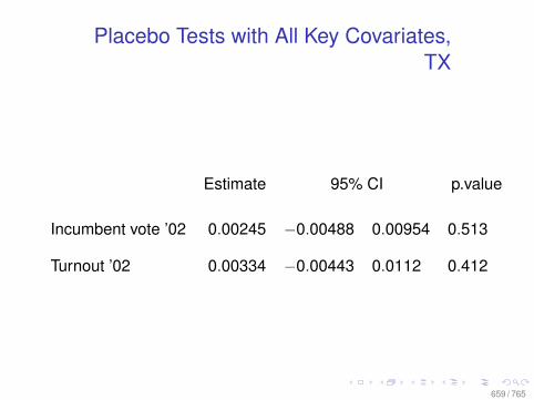
Placebo Tests with All Key Covariates,TX
Estimate 95% CI p.value
Incumbent vote ’02 0.00245 −0.00488 0.00954 0.513
Turnout ’02 0.00334 −0.00443 0.0112 0.412
659 / 765
Placebo Test TX: Presidential vote only
What happens if placebo test is done matching on presidentialvote only?• Achieve excellent balance on 2000 presidential vote• But there is still a significant effect in 2002, before
redistricting occurs• Past presidential vote is not sufficient to satisfy this
placebo test.• The significant effect estimated in the placebo test includes
the actual estimate of Ansolabehere, Snyder, and Stewart(2000) in its confidence interval.
660 / 765
Placebo Test TX: Presidential vote only
What happens if placebo test is done matching on presidentialvote only?• Achieve excellent balance on 2000 presidential vote• But there is still a significant effect in 2002, before
redistricting occurs• Past presidential vote is not sufficient to satisfy this
placebo test.• The significant effect estimated in the placebo test includes
the actual estimate of Ansolabehere, Snyder, and Stewart(2000) in its confidence interval.
661 / 765
Placebo Test TX: Presidential vote only
What happens if placebo test is done matching on presidentialvote only?• Achieve excellent balance on 2000 presidential vote• But there is still a significant effect in 2002, before
redistricting occurs• Past presidential vote is not sufficient to satisfy this
placebo test.• The significant effect estimated in the placebo test includes
the actual estimate of Ansolabehere, Snyder, and Stewart(2000) in its confidence interval.
662 / 765
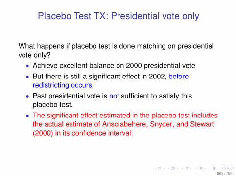
Placebo Test TX: Presidential vote only
What happens if placebo test is done matching on presidentialvote only?• Achieve excellent balance on 2000 presidential vote• But there is still a significant effect in 2002, before
redistricting occurs• Past presidential vote is not sufficient to satisfy this
placebo test.• The significant effect estimated in the placebo test includes
the actual estimate of Ansolabehere, Snyder, and Stewart(2000) in its confidence interval.
663 / 765
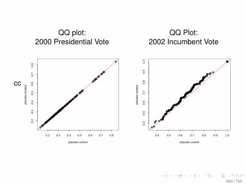
cc
QQ plot:2000 Presidential Vote
0.2 0.3 0.4 0.5 0.6 0.7 0.8
0.2
0.3
0.4
0.5
0.6
0.7
0.8
placebo control
plac
ebo
trea
ted
QQ Plot:2002 Incumbent Vote
0.4 0.5 0.6 0.7 0.8 0.9 1.0
0.4
0.5
0.6
0.7
0.8
0.9
1.0
placebo control
plac
ebo
trea
ted
664 / 765
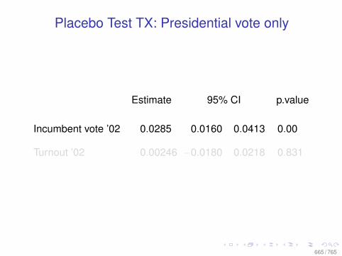
Placebo Test TX: Presidential vote only
Estimate 95% CI p.value
Incumbent vote ’02 0.0285 0.0160 0.0413 0.00
Turnout ’02 0.00246 −0.0180 0.0218 0.831
665 / 765
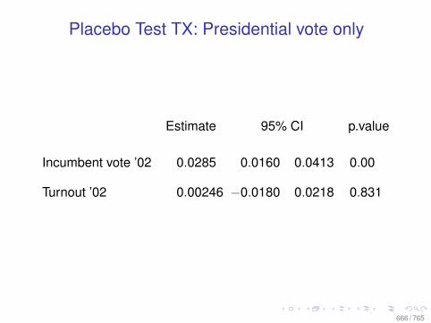
Placebo Test TX: Presidential vote only
Estimate 95% CI p.value
Incumbent vote ’02 0.0285 0.0160 0.0413 0.00
Turnout ’02 0.00246 −0.0180 0.0218 0.831
666 / 765
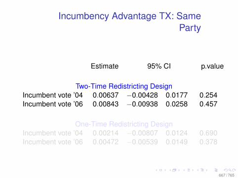
Incumbency Advantage TX: SameParty
Estimate 95% CI p.value
Two-Time Redistricting DesignIncumbent vote ’04 0.00637 −0.00428 0.0177 0.254Incumbent vote ’06 0.00843 −0.00938 0.0258 0.457
One-Time Redistricting DesignIncumbent vote ’04 0.00214 −0.00807 0.0124 0.690Incumbent vote ’06 0.00472 −0.00539 0.0149 0.378
667 / 765
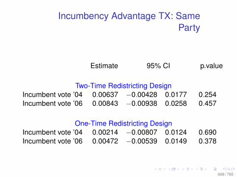
Incumbency Advantage TX: SameParty
Estimate 95% CI p.value
Two-Time Redistricting DesignIncumbent vote ’04 0.00637 −0.00428 0.0177 0.254Incumbent vote ’06 0.00843 −0.00938 0.0258 0.457
One-Time Redistricting DesignIncumbent vote ’04 0.00214 −0.00807 0.0124 0.690Incumbent vote ’06 0.00472 −0.00539 0.0149 0.378
668 / 765
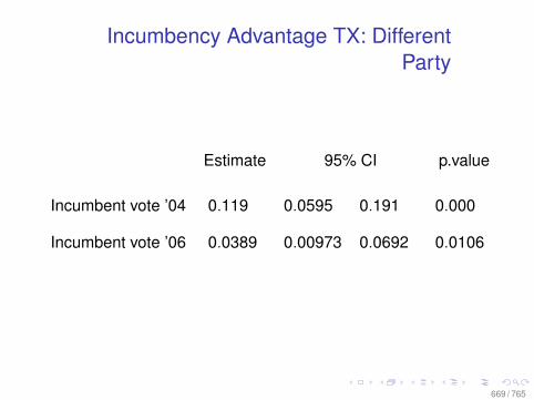
Incumbency Advantage TX: DifferentParty
Estimate 95% CI p.value
Incumbent vote ’04 0.119 0.0595 0.191 0.000
Incumbent vote ’06 0.0389 0.00973 0.0692 0.0106
669 / 765
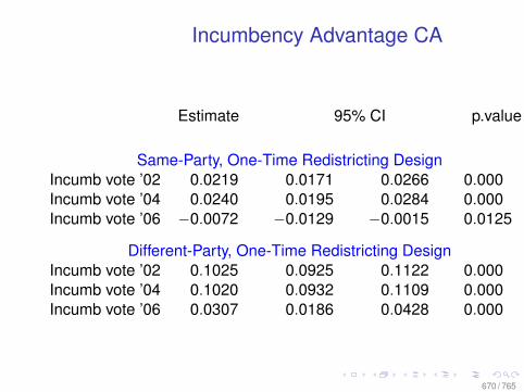
Incumbency Advantage CA
Estimate 95% CI p.value
Same-Party, One-Time Redistricting DesignIncumb vote ’02 0.0219 0.0171 0.0266 0.000Incumb vote ’04 0.0240 0.0195 0.0284 0.000Incumb vote ’06 −0.0072 −0.0129 −0.0015 0.0125
Different-Party, One-Time Redistricting DesignIncumb vote ’02 0.1025 0.0925 0.1122 0.000Incumb vote ’04 0.1020 0.0932 0.1109 0.000Incumb vote ’06 0.0307 0.0186 0.0428 0.000
670 / 765
Summary
• Our results are consistent with theoretical arguments thatexisting positive estimates are plagued by selectionproblems (Ashworth and Bueno de Mesquita, 2007;G. W. Cox and Katz, 2002; J. Zaller, 1998).
• Voters learn the type of new incumbent very quickly• Find a significant incumbent party effect. Consistent with
the results of Lee (2008).• Finding a positive incumbency effect is much less common
outside of the U.S. Some work even documents a negativeincumbency effect (Linden, 2004; Uppal, 2005).
671 / 765
Summary
• Our results are consistent with theoretical arguments thatexisting positive estimates are plagued by selectionproblems (Ashworth and Bueno de Mesquita, 2007;G. W. Cox and Katz, 2002; J. Zaller, 1998).
• Voters learn the type of new incumbent very quickly• Find a significant incumbent party effect. Consistent with
the results of Lee (2008).• Finding a positive incumbency effect is much less common
outside of the U.S. Some work even documents a negativeincumbency effect (Linden, 2004; Uppal, 2005).
672 / 765
Summary
• Our results are consistent with theoretical arguments thatexisting positive estimates are plagued by selectionproblems (Ashworth and Bueno de Mesquita, 2007;G. W. Cox and Katz, 2002; J. Zaller, 1998).
• Voters learn the type of new incumbent very quickly• Find a significant incumbent party effect. Consistent with
the results of Lee (2008).• Finding a positive incumbency effect is much less common
outside of the U.S. Some work even documents a negativeincumbency effect (Linden, 2004; Uppal, 2005).
673 / 765
A Cautionary Tale
• This should be an easy problem: clear question, a lot ofdata, and what people thought was a clean identificationstrategy
• “Natural experiments” require careful theoretical andstatistical work to make valid inferences
• Real experiments require that researchers a priori designthe study so that randomization will ensure theidentification of the causal effect
• Different ideal experiments imply different identifyingassumptions and hence different experimental designs
674 / 765
A Cautionary Tale
• This should be an easy problem: clear question, a lot ofdata, and what people thought was a clean identificationstrategy
• “Natural experiments” require careful theoretical andstatistical work to make valid inferences
• Real experiments require that researchers a priori designthe study so that randomization will ensure theidentification of the causal effect
• Different ideal experiments imply different identifyingassumptions and hence different experimental designs
675 / 765
A Cautionary Tale
• This should be an easy problem: clear question, a lot ofdata, and what people thought was a clean identificationstrategy
• “Natural experiments” require careful theoretical andstatistical work to make valid inferences
• Real experiments require that researchers a priori designthe study so that randomization will ensure theidentification of the causal effect
• Different ideal experiments imply different identifyingassumptions and hence different experimental designs
676 / 765
Hodges-Lehmann estimator
• Assume additive treatment effect• Subtract the hypothesized treatment effect from the treated
responses, and test hypothesis using these adjustedresponses
• Hodges-Lehmann (HL) estimate is the value that whensubtracted from the responses yields adjusted responsesthat are free of treatment effect, in the sense that the(Wilcoxon Signed Rank) test statistic equals its expectationin the absence of treatment effect
• Wilcoxon Signed Rank test statistic: form matchedtreated-control pairs, rank absolute value of treated-controldifferences within matched pairs, sum ranks for pairs inwhich treated response is higher than control response
677 / 765
Hodges-Lehmann estimator
• Assume additive treatment effect• Subtract the hypothesized treatment effect from the treated
responses, and test hypothesis using these adjustedresponses
• Hodges-Lehmann (HL) estimate is the value that whensubtracted from the responses yields adjusted responsesthat are free of treatment effect, in the sense that the(Wilcoxon Signed Rank) test statistic equals its expectationin the absence of treatment effect
• Wilcoxon Signed Rank test statistic: form matchedtreated-control pairs, rank absolute value of treated-controldifferences within matched pairs, sum ranks for pairs inwhich treated response is higher than control response
678 / 765
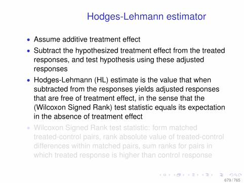
Hodges-Lehmann estimator
• Assume additive treatment effect• Subtract the hypothesized treatment effect from the treated
responses, and test hypothesis using these adjustedresponses
• Hodges-Lehmann (HL) estimate is the value that whensubtracted from the responses yields adjusted responsesthat are free of treatment effect, in the sense that the(Wilcoxon Signed Rank) test statistic equals its expectationin the absence of treatment effect
• Wilcoxon Signed Rank test statistic: form matchedtreated-control pairs, rank absolute value of treated-controldifferences within matched pairs, sum ranks for pairs inwhich treated response is higher than control response
679 / 765

Hodges-Lehmann estimator
• Assume additive treatment effect• Subtract the hypothesized treatment effect from the treated
responses, and test hypothesis using these adjustedresponses
• Hodges-Lehmann (HL) estimate is the value that whensubtracted from the responses yields adjusted responsesthat are free of treatment effect, in the sense that the(Wilcoxon Signed Rank) test statistic equals its expectationin the absence of treatment effect
• Wilcoxon Signed Rank test statistic: form matchedtreated-control pairs, rank absolute value of treated-controldifferences within matched pairs, sum ranks for pairs inwhich treated response is higher than control response
680 / 765
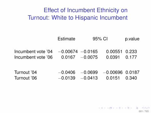
Effect of Incumbent Ethnicity onTurnout: White to Hispanic Incumbent
Estimate 95% CI p.value
Incumbent vote ’04 −0.00674 −0.0165 0.00551 0.233Incumbent vote ’06 0.0167 −0.0075 0.0391 0.177
Turnout ’04 −0.0406 −0.0699 −0.00696 0.0187Turnout ’06 −0.0139 −0.0413 0.0151 0.340
681 / 765
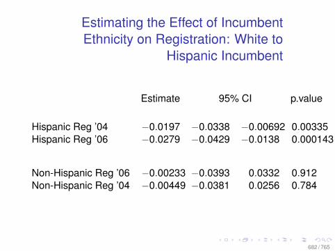
Estimating the Effect of IncumbentEthnicity on Registration: White to
Hispanic Incumbent
Estimate 95% CI p.value
Hispanic Reg ’04 −0.0197 −0.0338 −0.00692 0.00335Hispanic Reg ’06 −0.0279 −0.0429 −0.0138 0.000143
Non-Hispanic Reg ’06 −0.00233 −0.0393 0.0332 0.912Non-Hispanic Reg ’04 −0.00449 −0.0381 0.0256 0.784
682 / 765
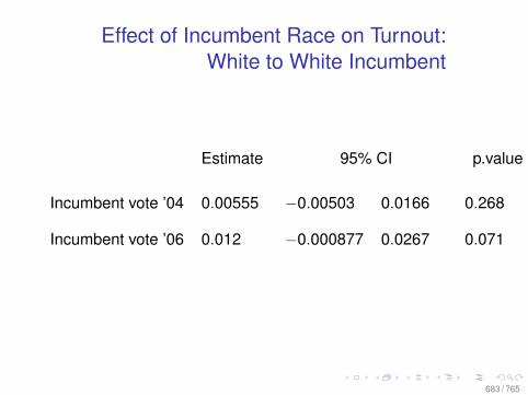
Effect of Incumbent Race on Turnout:White to White Incumbent
Estimate 95% CI p.value
Incumbent vote ’04 0.00555 −0.00503 0.0166 0.268
Incumbent vote ’06 0.012 −0.000877 0.0267 0.071
683 / 765
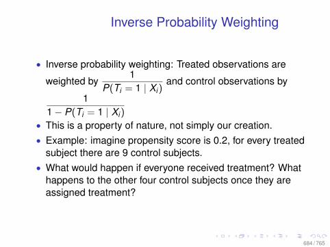
Inverse Probability Weighting
• Inverse probability weighting: Treated observations are
weighted by1
P(Ti = 1 | Xi)and control observations by
11− P(Ti = 1 | Xi)
• This is a property of nature, not simply our creation.• Example: imagine propensity score is 0.2, for every treated
subject there are 9 control subjects.• What would happen if everyone received treatment? What
happens to the other four control subjects once they areassigned treatment?
684 / 765
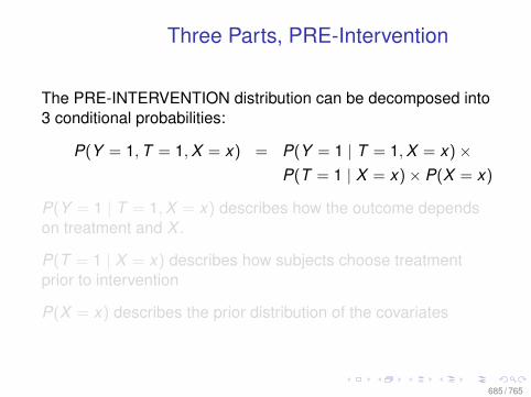
Three Parts, PRE-Intervention
The PRE-INTERVENTION distribution can be decomposed into3 conditional probabilities:
P(Y = 1,T = 1,X = x) = P(Y = 1 | T = 1,X = x)×P(T = 1 | X = x)× P(X = x)
P(Y = 1 | T = 1,X = x) describes how the outcome dependson treatment and X .
P(T = 1 | X = x) describes how subjects choose treatmentprior to intervention
P(X = x) describes the prior distribution of the covariates
685 / 765
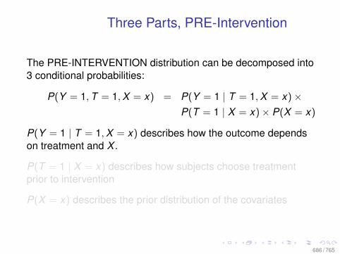
Three Parts, PRE-Intervention
The PRE-INTERVENTION distribution can be decomposed into3 conditional probabilities:
P(Y = 1,T = 1,X = x) = P(Y = 1 | T = 1,X = x)×P(T = 1 | X = x)× P(X = x)
P(Y = 1 | T = 1,X = x) describes how the outcome dependson treatment and X .
P(T = 1 | X = x) describes how subjects choose treatmentprior to intervention
P(X = x) describes the prior distribution of the covariates
686 / 765
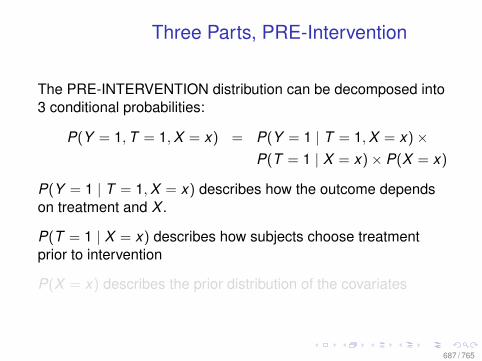
Three Parts, PRE-Intervention
The PRE-INTERVENTION distribution can be decomposed into3 conditional probabilities:
P(Y = 1,T = 1,X = x) = P(Y = 1 | T = 1,X = x)×P(T = 1 | X = x)× P(X = x)
P(Y = 1 | T = 1,X = x) describes how the outcome dependson treatment and X .
P(T = 1 | X = x) describes how subjects choose treatmentprior to intervention
P(X = x) describes the prior distribution of the covariates
687 / 765
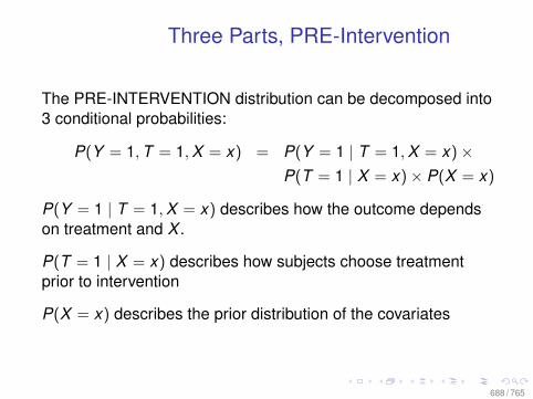
Three Parts, PRE-Intervention
The PRE-INTERVENTION distribution can be decomposed into3 conditional probabilities:
P(Y = 1,T = 1,X = x) = P(Y = 1 | T = 1,X = x)×P(T = 1 | X = x)× P(X = x)
P(Y = 1 | T = 1,X = x) describes how the outcome dependson treatment and X .
P(T = 1 | X = x) describes how subjects choose treatmentprior to intervention
P(X = x) describes the prior distribution of the covariates
688 / 765
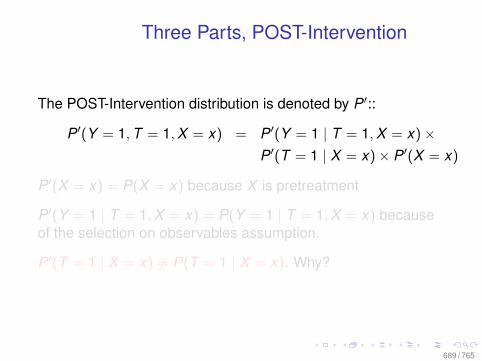
Three Parts, POST-Intervention
The POST-Intervention distribution is denoted by P ′::
P ′(Y = 1,T = 1,X = x) = P ′(Y = 1 | T = 1,X = x)×P ′(T = 1 | X = x)× P ′(X = x)
P ′(X = x) = P(X = x) because X is pretreatment
P ′(Y = 1 | T = 1,X = x) = P(Y = 1 | T = 1,X = x) becauseof the selection on observables assumption.
P ′(T = 1 | X = x) 6= P(T = 1 | X = x). Why?
689 / 765
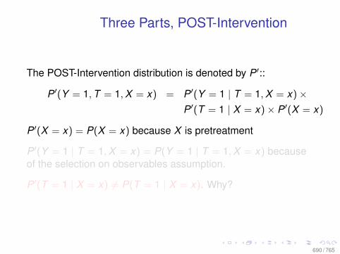
Three Parts, POST-Intervention
The POST-Intervention distribution is denoted by P ′::
P ′(Y = 1,T = 1,X = x) = P ′(Y = 1 | T = 1,X = x)×P ′(T = 1 | X = x)× P ′(X = x)
P ′(X = x) = P(X = x) because X is pretreatment
P ′(Y = 1 | T = 1,X = x) = P(Y = 1 | T = 1,X = x) becauseof the selection on observables assumption.
P ′(T = 1 | X = x) 6= P(T = 1 | X = x). Why?
690 / 765
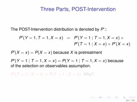
Three Parts, POST-Intervention
The POST-Intervention distribution is denoted by P ′::
P ′(Y = 1,T = 1,X = x) = P ′(Y = 1 | T = 1,X = x)×P ′(T = 1 | X = x)× P ′(X = x)
P ′(X = x) = P(X = x) because X is pretreatment
P ′(Y = 1 | T = 1,X = x) = P(Y = 1 | T = 1,X = x) becauseof the selection on observables assumption.
P ′(T = 1 | X = x) 6= P(T = 1 | X = x). Why?
691 / 765
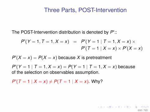
Three Parts, POST-Intervention
The POST-Intervention distribution is denoted by P ′::
P ′(Y = 1,T = 1,X = x) = P ′(Y = 1 | T = 1,X = x)×P ′(T = 1 | X = x)× P ′(X = x)
P ′(X = x) = P(X = x) because X is pretreatment
P ′(Y = 1 | T = 1,X = x) = P(Y = 1 | T = 1,X = x) becauseof the selection on observables assumption.
P ′(T = 1 | X = x) 6= P(T = 1 | X = x). Why?
692 / 765
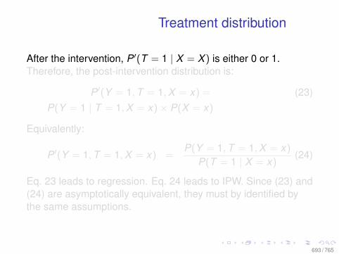
Treatment distribution
After the intervention, P ′(T = 1 | X = X ) is either 0 or 1.Therefore, the post-intervention distribution is:
P ′(Y = 1,T = 1,X = x) = (23)P(Y = 1 | T = 1,X = x)× P(X = x)
Equivalently:
P ′(Y = 1,T = 1,X = x) =P(Y = 1,T = 1,X = x)
P(T = 1 | X = x)(24)
Eq. 23 leads to regression. Eq. 24 leads to IPW. Since (23) and(24) are asymptotically equivalent, they must by identified bythe same assumptions.
693 / 765
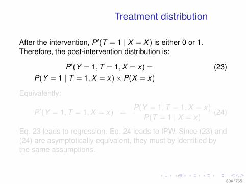
Treatment distribution
After the intervention, P ′(T = 1 | X = X ) is either 0 or 1.Therefore, the post-intervention distribution is:
P ′(Y = 1,T = 1,X = x) = (23)P(Y = 1 | T = 1,X = x)× P(X = x)
Equivalently:
P ′(Y = 1,T = 1,X = x) =P(Y = 1,T = 1,X = x)
P(T = 1 | X = x)(24)
Eq. 23 leads to regression. Eq. 24 leads to IPW. Since (23) and(24) are asymptotically equivalent, they must by identified bythe same assumptions.
694 / 765
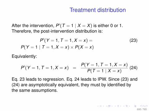
Treatment distribution
After the intervention, P ′(T = 1 | X = X ) is either 0 or 1.Therefore, the post-intervention distribution is:
P ′(Y = 1,T = 1,X = x) = (23)P(Y = 1 | T = 1,X = x)× P(X = x)
Equivalently:
P ′(Y = 1,T = 1,X = x) =P(Y = 1,T = 1,X = x)
P(T = 1 | X = x)(24)
Eq. 23 leads to regression. Eq. 24 leads to IPW. Since (23) and(24) are asymptotically equivalent, they must by identified bythe same assumptions.
695 / 765
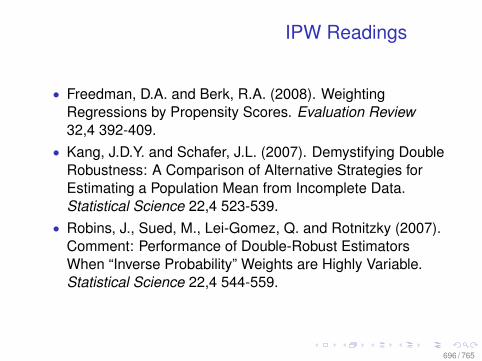
IPW Readings
• Freedman, D.A. and Berk, R.A. (2008). WeightingRegressions by Propensity Scores. Evaluation Review32,4 392-409.
• Kang, J.D.Y. and Schafer, J.L. (2007). Demystifying DoubleRobustness: A Comparison of Alternative Strategies forEstimating a Population Mean from Incomplete Data.Statistical Science 22,4 523-539.
• Robins, J., Sued, M., Lei-Gomez, Q. and Rotnitzky (2007).Comment: Performance of Double-Robust EstimatorsWhen “Inverse Probability” Weights are Highly Variable.Statistical Science 22,4 544-559.
696 / 765
Collaborative Targeted MaximumLikelihood
• Double robust estimator use knowledge of Y , but theyshow poor properties when the pscore is close to 0 or 1.
• Even if the pscore model is correct, one is often better offnot adjusted by the pscore and just modelling Y—e.g.,Freedman and Berk 2008
• Even true for bounded doubly robust estimators• Influence curve may be bounded, but MSE is still
increased by using the pscore• C-TMLE helps (van der Laan and Gruber 2009); extends
targeted ML• One can extend C-TMLE to trim data as matching
does—adjusted collaborative targeted maximum likelihood• Incorporate various ways of trimming including that of
Crump, Hotz, Imbens, and Mitnik (2006)697 / 765
Collaborative Targeted MaximumLikelihood
• Double robust estimator use knowledge of Y , but theyshow poor properties when the pscore is close to 0 or 1.
• Even if the pscore model is correct, one is often better offnot adjusted by the pscore and just modelling Y—e.g.,Freedman and Berk 2008
• Even true for bounded doubly robust estimators• Influence curve may be bounded, but MSE is still
increased by using the pscore• C-TMLE helps (van der Laan and Gruber 2009); extends
targeted ML• One can extend C-TMLE to trim data as matching
does—adjusted collaborative targeted maximum likelihood• Incorporate various ways of trimming including that of
Crump, Hotz, Imbens, and Mitnik (2006)698 / 765
Collaborative Targeted MaximumLikelihood
• Double robust estimator use knowledge of Y , but theyshow poor properties when the pscore is close to 0 or 1.
• Even if the pscore model is correct, one is often better offnot adjusted by the pscore and just modelling Y—e.g.,Freedman and Berk 2008
• Even true for bounded doubly robust estimators• Influence curve may be bounded, but MSE is still
increased by using the pscore• C-TMLE helps (van der Laan and Gruber 2009); extends
targeted ML• One can extend C-TMLE to trim data as matching
does—adjusted collaborative targeted maximum likelihood• Incorporate various ways of trimming including that of
Crump, Hotz, Imbens, and Mitnik (2006)699 / 765
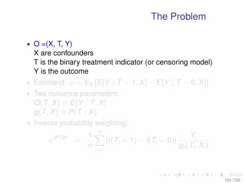
The Problem
• O =(X, T, Y)X are confoundersT is the binary treatment indicator (or censoring model)Y is the outcome
• Estimand: ψ = EX [E [Y | T = 1,X ]− E [Y | T = 0,X ]]
• Two nuisance parameters:Q(T ,X ) ≡ E [Y | T ,X ]g(T ,X ) ≡ P(T | X )
• Inverse probability weighting:
ψIPTW =1n
n∑i=1
[I(Ti = 1)− I(Ti = 0)]Yi
gn(Ti ,Xi)
700 / 765
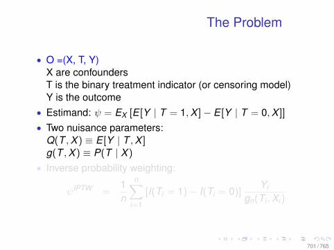
The Problem
• O =(X, T, Y)X are confoundersT is the binary treatment indicator (or censoring model)Y is the outcome
• Estimand: ψ = EX [E [Y | T = 1,X ]− E [Y | T = 0,X ]]
• Two nuisance parameters:Q(T ,X ) ≡ E [Y | T ,X ]g(T ,X ) ≡ P(T | X )
• Inverse probability weighting:
ψIPTW =1n
n∑i=1
[I(Ti = 1)− I(Ti = 0)]Yi
gn(Ti ,Xi)
701 / 765
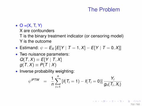
The Problem
• O =(X, T, Y)X are confoundersT is the binary treatment indicator (or censoring model)Y is the outcome
• Estimand: ψ = EX [E [Y | T = 1,X ]− E [Y | T = 0,X ]]
• Two nuisance parameters:Q(T ,X ) ≡ E [Y | T ,X ]g(T ,X ) ≡ P(T | X )
• Inverse probability weighting:
ψIPTW =1n
n∑i=1
[I(Ti = 1)− I(Ti = 0)]Yi
gn(Ti ,Xi)
702 / 765
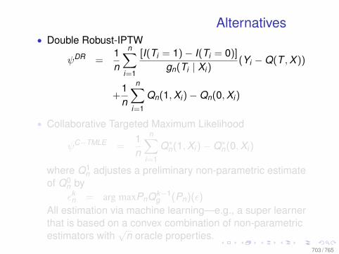
Alternatives• Double Robust-IPTW
ψDR =1n
n∑i=1
[I(Ti = 1)− I(Ti = 0)]
gn(Ti | Xi)(Yi −Q(T ,X ))
+1n
n∑i=1
Qn(1,Xi)−Qn(0,Xi)
• Collaborative Targeted Maximum Likelihood
ψC−TMLE =1n
n∑i=1
Q∗n(1,Xi)−Q∗n(0,Xi)
where Q1n adjustes a preliminary non-parametric estimate
of Q0n byεkn = arg maxPnQk−1
g (Pn)(ε)
All estimation via machine learning—e.g., a super learnerthat is based on a convex combination of non-parametricestimators with
√n oracle properties.
703 / 765
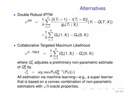
Alternatives• Double Robust-IPTW
ψDR =1n
n∑i=1
[I(Ti = 1)− I(Ti = 0)]
gn(Ti | Xi)(Yi −Q(T ,X ))
+1n
n∑i=1
Qn(1,Xi)−Qn(0,Xi)
• Collaborative Targeted Maximum Likelihood
ψC−TMLE =1n
n∑i=1
Q∗n(1,Xi)−Q∗n(0,Xi)
where Q1n adjustes a preliminary non-parametric estimate
of Q0n byεkn = arg maxPnQk−1
g (Pn)(ε)
All estimation via machine learning—e.g., a super learnerthat is based on a convex combination of non-parametricestimators with
√n oracle properties.
704 / 765
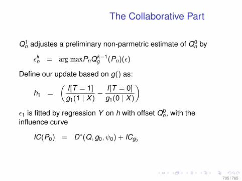
The Collaborative Part
Q1n adjustes a preliminary non-parmetric estimate of Q0
n by
εkn = arg maxPnQk−1g (Pn)(ε)
Define our update based on g() as:
h1 =
(I[T = 1]
g1(1 | X )− I[T = 0]
g1(0 | X )
)ε1 is fitted by regression Y on h with offset Q0
n , with theinfluence curve
IC(P0) = D∗(Q,g0, ψ0) + ICg0
705 / 765
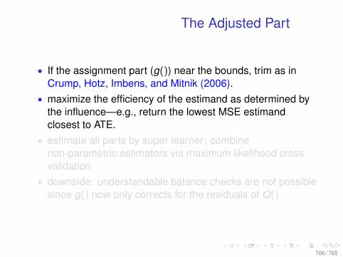
The Adjusted Part
• If the assignment part (g()) near the bounds, trim as inCrump, Hotz, Imbens, and Mitnik (2006).
• maximize the efficiency of the estimand as determined bythe influence—e.g., return the lowest MSE estimandclosest to ATE.
• estimate all parts by super learner: combinenon-parametric estimators via maximum likelihood crossvalidation
• downside: understandable balance checks are not possiblesince g() now only corrects for the residuals of Q()
706 / 765
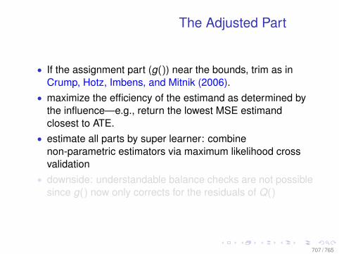
The Adjusted Part
• If the assignment part (g()) near the bounds, trim as inCrump, Hotz, Imbens, and Mitnik (2006).
• maximize the efficiency of the estimand as determined bythe influence—e.g., return the lowest MSE estimandclosest to ATE.
• estimate all parts by super learner: combinenon-parametric estimators via maximum likelihood crossvalidation
• downside: understandable balance checks are not possiblesince g() now only corrects for the residuals of Q()
707 / 765
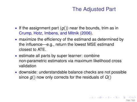
The Adjusted Part
• If the assignment part (g()) near the bounds, trim as inCrump, Hotz, Imbens, and Mitnik (2006).
• maximize the efficiency of the estimand as determined bythe influence—e.g., return the lowest MSE estimandclosest to ATE.
• estimate all parts by super learner: combinenon-parametric estimators via maximum likelihood crossvalidation
• downside: understandable balance checks are not possiblesince g() now only corrects for the residuals of Q()
708 / 765
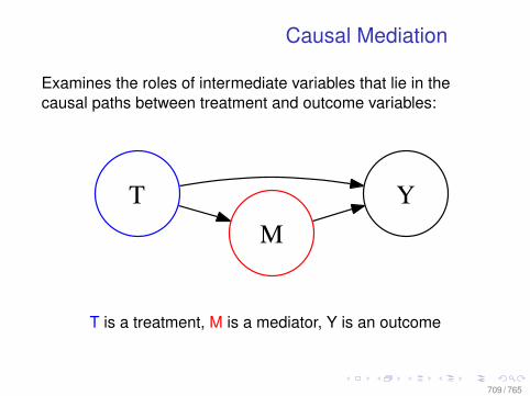
Causal Mediation
Examines the roles of intermediate variables that lie in thecausal paths between treatment and outcome variables:
YTM
T is a treatment, M is a mediator, Y is an outcome
709 / 765
Mediation Analysis is Popular
• Researchers want to know how and why treatment has aneffect not simply that it does
• Very popular—e.g., Baron and Kenny (1986), cited 19,988times. Linear version goes back to Haavelmo (1943) andSimon (1943)
• New assumptions have been proposed that providenonparametric identification—e.g., Robins and Greenland(1992), Pearl (2001), Robins (2003), Petersen, Sinisi andvan der Laan (2006), Hafeman and VanderWeele (2010),Imai et al. (2010).
710 / 765
Mediation Analysis is Problematic
• These assumptions are usually implausible• I provide analytical results which demonstrate that these
assumptions are fragile: when the assumptions are slightlyweakened, identification is lost
• Troubling because researchers claim it is essential toestimate causal mediation effects to test substantivetheories
711 / 765

Example: Religious Practice in India
• Joint work with Pradeep Chhibber• Do Muslims political leaders have greater trust in a political
context than other religious leaders?• Can leaders use religious symbols to politically mobilize
supporters?• We are especially interested in differences between
Muslims and Hindus• Religious practice differs sharply between Muslims and
Hindus, and between Sunnis and Shiites• Conjecture: Islamic religious leaders, particularly Sunni,
have greater political role than Hindu religious leaders
712 / 765

Example: Religious Practice in India
• Joint work with Pradeep Chhibber• Do Muslims political leaders have greater trust in a political
context than other religious leaders?• Can leaders use religious symbols to politically mobilize
supporters?• We are especially interested in differences between
Muslims and Hindus• Religious practice differs sharply between Muslims and
Hindus, and between Sunnis and Shiites• Conjecture: Islamic religious leaders, particularly Sunni,
have greater political role than Hindu religious leaders
713 / 765

Why People Care?
Current Question:• Concern about the role of Imams in radicalization• This role may vary across different Islamic groups and
contexts
Historical Question:• Long running debate on the political role of Imams. Islamic
organization was never centralized—no Pope.• But Christians and Muslim both regularly launched
cross-continental crusades in the last millennium.
714 / 765

Why People Care?
Current Question:• Concern about the role of Imams in radicalization• This role may vary across different Islamic groups and
contexts
Historical Question:• Long running debate on the political role of Imams. Islamic
organization was never centralized—no Pope.• But Christians and Muslim both regularly launched
cross-continental crusades in the last millennium.
715 / 765
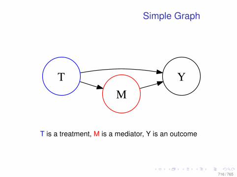
Simple Graph
YTM
T is a treatment, M is a mediator, Y is an outcome
716 / 765
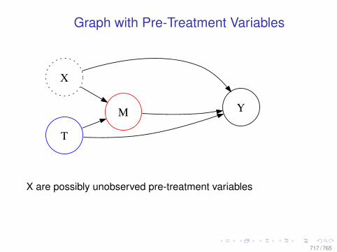
Graph with Pre-Treatment Variables
X
M YZ
T
X are possibly unobserved pre-treatment variables
717 / 765
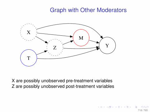
Graph with Other Moderators
XM
YZ
T
X are possibly unobserved pre-treatment variablesZ are possibly unobserved post-treatment variables
718 / 765
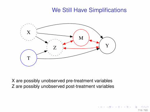
We Still Have Simplifications
XM
YZ
T
X are possibly unobserved pre-treatment variablesZ are possibly unobserved post-treatment variables
719 / 765
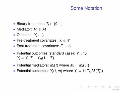
Some Notation
• Binary treatment: Ti ∈ 0,1• Mediator: Mi ∈M• Outcome: Yi ∈ Y• Pre-treatment covariates: Xi ∈ X• Post-treatment covariates: Zi ∈ Z
• Potential outcomes (standard case): Yi1,Yi0,Yi = Yi1T + Yi0(1− T )
• Potential mediators: Mi(t) where Mi = Mi(Ti)
• Potential outcomes: Yi(t ,m) where Yi = Y (Ti ,Mi(Ti))
720 / 765
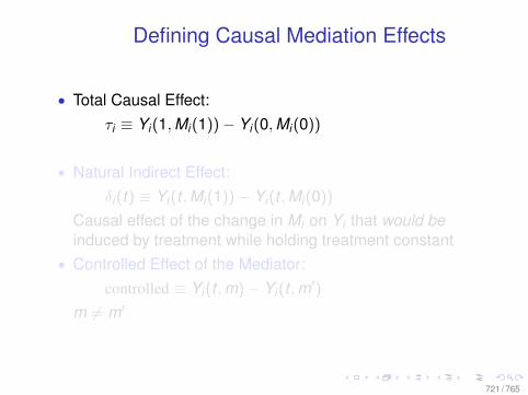
Defining Causal Mediation Effects
• Total Causal Effect:τi ≡ Yi(1,Mi(1))− Yi(0,Mi(0))
• Natural Indirect Effect:δi(t) ≡ Yi(t ,Mi(1))− Yi(t ,Mi(0))
Causal effect of the change in Mi on Yi that would beinduced by treatment while holding treatment constant
• Controlled Effect of the Mediator:controlled ≡ Yi(t ,m)− Yi(t ,m′)
m 6= m′
721 / 765
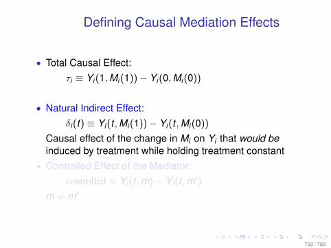
Defining Causal Mediation Effects
• Total Causal Effect:τi ≡ Yi(1,Mi(1))− Yi(0,Mi(0))
• Natural Indirect Effect:δi(t) ≡ Yi(t ,Mi(1))− Yi(t ,Mi(0))
Causal effect of the change in Mi on Yi that would beinduced by treatment while holding treatment constant
• Controlled Effect of the Mediator:controlled ≡ Yi(t ,m)− Yi(t ,m′)
m 6= m′
722 / 765
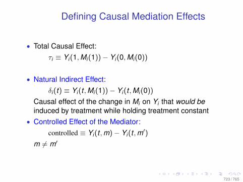
Defining Causal Mediation Effects
• Total Causal Effect:τi ≡ Yi(1,Mi(1))− Yi(0,Mi(0))
• Natural Indirect Effect:δi(t) ≡ Yi(t ,Mi(1))− Yi(t ,Mi(0))
Causal effect of the change in Mi on Yi that would beinduced by treatment while holding treatment constant
• Controlled Effect of the Mediator:controlled ≡ Yi(t ,m)− Yi(t ,m′)
m 6= m′
723 / 765
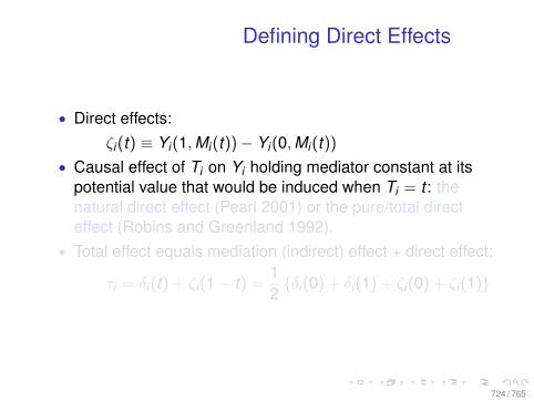
Defining Direct Effects
• Direct effects:ζi(t) ≡ Yi(1,Mi(t))− Yi(0,Mi(t))
• Causal effect of Ti on Yi holding mediator constant at itspotential value that would be induced when Ti = t : thenatural direct effect (Pearl 2001) or the pure/total directeffect (Robins and Greenland 1992).
• Total effect equals mediation (indirect) effect + direct effect:
τi = δi(t) + ζi(1− t) =12δi(0) + δi(1) + ζi(0) + ζi(1)
724 / 765
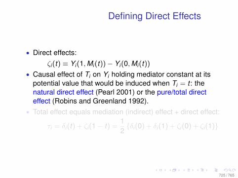
Defining Direct Effects
• Direct effects:ζi(t) ≡ Yi(1,Mi(t))− Yi(0,Mi(t))
• Causal effect of Ti on Yi holding mediator constant at itspotential value that would be induced when Ti = t : thenatural direct effect (Pearl 2001) or the pure/total directeffect (Robins and Greenland 1992).
• Total effect equals mediation (indirect) effect + direct effect:
τi = δi(t) + ζi(1− t) =12δi(0) + δi(1) + ζi(0) + ζi(1)
725 / 765
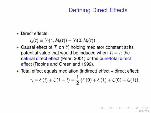
Defining Direct Effects
• Direct effects:ζi(t) ≡ Yi(1,Mi(t))− Yi(0,Mi(t))
• Causal effect of Ti on Yi holding mediator constant at itspotential value that would be induced when Ti = t : thenatural direct effect (Pearl 2001) or the pure/total directeffect (Robins and Greenland 1992).
• Total effect equals mediation (indirect) effect + direct effect:
τi = δi(t) + ζi(1− t) =12δi(0) + δi(1) + ζi(0) + ζi(1)
726 / 765

Identification of Average CausalMediation Effect
• Average Causal Mediation Effect (ACME):δ(t) ≡ E(δi(t)) = E Yi(t ,Mi(1))− Yi(t ,Mi(0))
• Issue: we can never observe Yi(t ,Mi(1− t))
• One assumption, Sequential Ignorability (e.g., Imai et al.2010):
Yi(t ′,m),Mi(t)
⊥⊥ Ti | Xi = x (25)
Yi(t ′,m) ⊥⊥ Mi(t) | Ti = t ,Xi = x , (26)
for t , t ′ = 0,1; 0 < Pr(Ti = t | Xi = x) and0 < p(Mi = m | Ti = t ,Xi = x), ∀ x ∈ X and m ∈ M
727 / 765
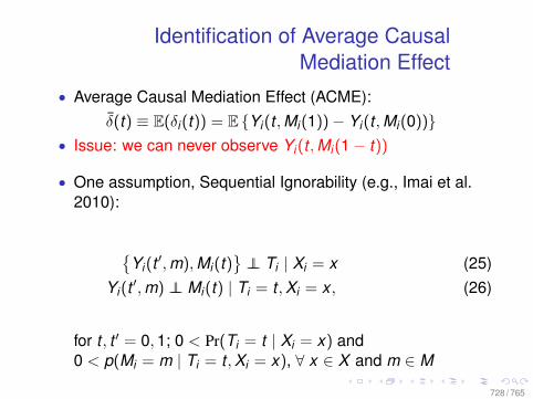
Identification of Average CausalMediation Effect
• Average Causal Mediation Effect (ACME):δ(t) ≡ E(δi(t)) = E Yi(t ,Mi(1))− Yi(t ,Mi(0))
• Issue: we can never observe Yi(t ,Mi(1− t))
• One assumption, Sequential Ignorability (e.g., Imai et al.2010):
Yi(t ′,m),Mi(t)
⊥⊥ Ti | Xi = x (25)
Yi(t ′,m) ⊥⊥ Mi(t) | Ti = t ,Xi = x , (26)
for t , t ′ = 0,1; 0 < Pr(Ti = t | Xi = x) and0 < p(Mi = m | Ti = t ,Xi = x), ∀ x ∈ X and m ∈ M
728 / 765
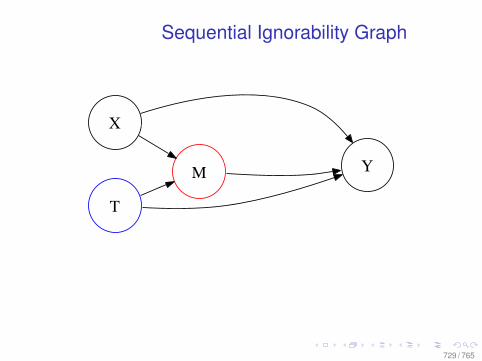
Sequential Ignorability Graph
X
M YZ
T
729 / 765
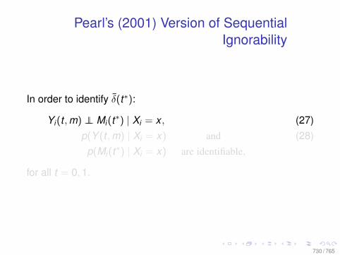
Pearl’s (2001) Version of SequentialIgnorability
In order to identify δ(t∗):
Yi(t ,m) ⊥⊥ Mi(t∗) | Xi = x , (27)p(Y (t ,m) | Xi = x) and (28)
p(Mi(t∗) | Xi = x) are identifiable,
for all t = 0,1.
730 / 765
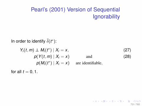
Pearl’s (2001) Version of SequentialIgnorability
In order to identify δ(t∗):
Yi(t ,m) ⊥⊥ Mi(t∗) | Xi = x , (27)p(Y (t ,m) | Xi = x) and (28)
p(Mi(t∗) | Xi = x) are identifiable,
for all t = 0,1.
731 / 765
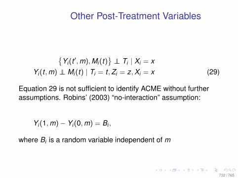
Other Post-Treatment Variables
Yi(t ′,m),Mi(t)
⊥⊥ Ti | Xi = x
Yi(t ,m) ⊥⊥ Mi(t) | Ti = t ,Zi = z,Xi = x (29)
Equation 29 is not sufficient to identify ACME without furtherassumptions. Robins’ (2003) “no-interaction” assumption:
Yi(1,m)− Yi(0,m) = Bi ,
where Bi is a random variable independent of m
732 / 765
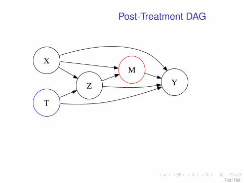
Post-Treatment DAG
XM
YZ
T
733 / 765
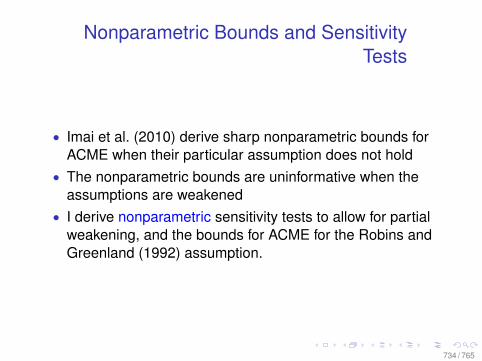
Nonparametric Bounds and SensitivityTests
• Imai et al. (2010) derive sharp nonparametric bounds forACME when their particular assumption does not hold
• The nonparametric bounds are uninformative when theassumptions are weakened
• I derive nonparametric sensitivity tests to allow for partialweakening, and the bounds for ACME for the Robins andGreenland (1992) assumption.
734 / 765
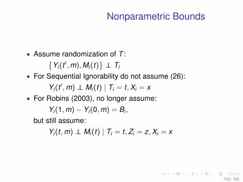
Nonparametric Bounds
• Assume randomization of T :Yi(t ′,m),Mi(t)
⊥⊥ Ti
• For Sequential Ignorability do not assume (26):Yi(t ′,m) ⊥⊥ Mi(t) | Ti = t ,Xi = x
• For Robins (2003), no longer assume:Yi(1,m)− Yi(0,m) = Bi ,
but still assume:Yi(t ,m) ⊥⊥ Mi(t) | Ti = t ,Zi = z,Xi = x
735 / 765
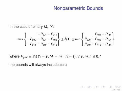
Nonparametric Bounds
In the case of binary M, Y :
max
−P001 − P011
−P000 − P001 − P100
−P011 − P010 − P110
≤ δ(1) ≤ min
P101 + P111
P000 + P100 + P101
P010 + P110 + P111
where Pymt ≡ Pr(Yi = y ,Mi = m | Ti = t), ∀ y ,m, t ∈ 0,1
the bounds will always include zero
736 / 765
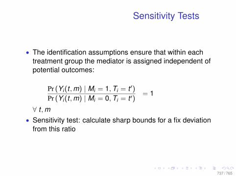
Sensitivity Tests
• The identification assumptions ensure that within eachtreatment group the mediator is assigned independent ofpotential outcomes:
Pr (Yi(t ,m) | Mi = 1,Ti = t ′)Pr (Yi(t ,m) | Mi = 0,Ti = t ′)
= 1
∀ t ,m• Sensitivity test: calculate sharp bounds for a fix deviation
from this ratio
737 / 765
A Series of Experiments
• Measure reported trust in political leaders, randomizereligious versus secular leaders
• Prompt people to vote, randomize religious versus secularprompt. Measure voter turnout and vote.
• Conduct experiments on different groups (Sunni/Shiite,Hindus, Sikhs) and at different locations (majority/minority)
• Natural experiment: Iranian Shiite Imams in Afghanistan• More Experiments: Governments
738 / 765
A Series of Experiments
• Measure reported trust in political leaders, randomizereligious versus secular leaders
• Prompt people to vote, randomize religious versus secularprompt. Measure voter turnout and vote.
• Conduct experiments on different groups (Sunni/Shiite,Hindus, Sikhs) and at different locations (majority/minority)
• Natural experiment: Iranian Shiite Imams in Afghanistan• More Experiments: Governments
739 / 765

Example Photos
740 / 765

Simple Trust Experiment
At a recent meeting celebrating India’s democracy this leadingpolitician (show photo) said:
“Politicians like me from different political parties tryhard to represent the interests of the people whosupport us and vote for us.”
Do you think he can be trusted?
741 / 765

Trust in Uttar Pradesh
Muslim Hindu
UP, Aligarh
Estimate 15.1% 3.79%p-value 0.000686 0.387
UP, Kanpur
Estimate 12.6% -1.20%p-value 0.0118 0.791
742 / 765
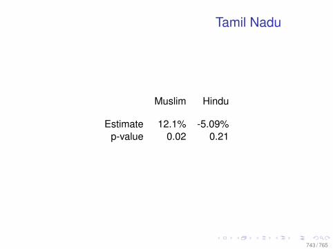
Tamil Nadu
Muslim Hindu
Estimate 12.1% -5.09%p-value 0.02 0.21
743 / 765

Shiite Muslims
Uttar Pradesh, Lucknow
Muslim Hindu
Estimate 4.80% 4.72%p-value 0.337 0.336
744 / 765
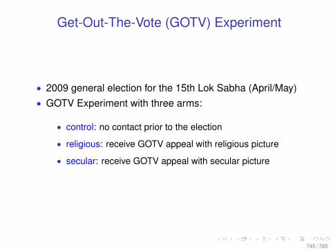
Get-Out-The-Vote (GOTV) Experiment
• 2009 general election for the 15th Lok Sabha (April/May)• GOTV Experiment with three arms:
• control: no contact prior to the election
• religious: receive GOTV appeal with religious picture
• secular: receive GOTV appeal with secular picture
745 / 765

Non-Religious Leader Appeal
This learned person has written a book. The book says thatPolitics affects whether the government looks after the interestsof people like you and the interests of your community. Heurged everyone to VOTE!
He wrote that if you as a citizen want to have your input inmaking politics and government work for your community, youneed to VOTE in order to send a message to those in power.Your interests and the interests of your community will not beattended to if you do not VOTE.
746 / 765
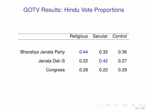
GOTV Results: Hindu Vote Proportions
Religious Secular Control
Bharatiya Janata Party 0.44 0.32 0.36
Janata Dal–S 0.22 0.42 0.27
Congress 0.28 0.22 0.29
747 / 765
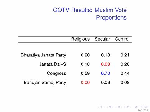
GOTV Results: Muslim VoteProportions
Religious Secular Control
Bharatiya Janata Party 0.20 0.18 0.21
Janata Dal–S 0.18 0.03 0.26
Congress 0.59 0.70 0.44
Bahujan Samaj Party 0.00 0.06 0.08
748 / 765

Other Experiments: Triangulation
• Iranian Shiite Imams in Afghanistan, a natural experimentduring Muharram
• Public Safety Canada: Doing things Berkeley won’t
749 / 765
Conclusion
• Triangulation will never be logically sufficient
• Many moving parts: political trust, voting, the strategicrelationship between political parties, majority/minority,Shiite vs. Sunni, levels of violence, media saturation
• The temptation of reductionism is widespread: logicalpositivism, a common language in which all scientificpropositions can be expressed
• Causality and manipulation are separable concepts
750 / 765
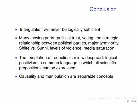
Conclusion
• Triangulation will never be logically sufficient
• Many moving parts: political trust, voting, the strategicrelationship between political parties, majority/minority,Shiite vs. Sunni, levels of violence, media saturation
• The temptation of reductionism is widespread: logicalpositivism, a common language in which all scientificpropositions can be expressed
• Causality and manipulation are separable concepts
751 / 765
Manipulation and Reductionism
• A good Mantra: “No causation without manipulation”• But this does not imply the Dogma of reductionism
common in the literature• Classic Example:
• Incoherent: “What is the causal effect of being white onincome/grades/happiness?”
• But this does not imply that race does not play a role ingenerating these outcomes
• We test theories of how different religions are organized.Do Imams have a greater political role than other religiousleaders? Are they more trusted?
752 / 765
Manipulation and Reductionism
• A good Mantra: “No causation without manipulation”• But this does not imply the Dogma of reductionism
common in the literature• Classic Example:
• Incoherent: “What is the causal effect of being white onincome/grades/happiness?”
• But this does not imply that race does not play a role ingenerating these outcomes
• We test theories of how different religions are organized.Do Imams have a greater political role than other religiousleaders? Are they more trusted?
753 / 765
Manipulation and Reductionism
• A good Mantra: “No causation without manipulation”• But this does not imply the Dogma of reductionism
common in the literature• Classic Example:
• Incoherent: “What is the causal effect of being white onincome/grades/happiness?”
• But this does not imply that race does not play a role ingenerating these outcomes
• We test theories of how different religions are organized.Do Imams have a greater political role than other religiousleaders? Are they more trusted?
754 / 765
Manipulation and Reductionism
• A good Mantra: “No causation without manipulation”• But this does not imply the Dogma of reductionism
common in the literature• Classic Example:
• Incoherent: “What is the causal effect of being white onincome/grades/happiness?”
• But this does not imply that race does not play a role ingenerating these outcomes
• We test theories of how different religions are organized.Do Imams have a greater political role than other religiousleaders? Are they more trusted?
755 / 765

What is Reductionism?
• Extreme Reductionism: every scientific sentence has a fulltranslation in sense-datum
• Moderate Reductionism: each scientific sentence has itsown separate empirical content
• Moderate Holism: a scientific sentence need not implyempirical consequences by itself. A bigger cluster isusually needed.
• Classic Example: Copernican vs. Ptolemaic system. Betterexample: Aryabhat.a (500CE)—diurnal motion of the earth,elliptic orbits calculated relative to the sun, correctexplanation of lunar and solar eclipses, but still geocentric.
756 / 765
What is Reductionism?
• Extreme Reductionism: every scientific sentence has a fulltranslation in sense-datum
• Moderate Reductionism: each scientific sentence has itsown separate empirical content
• Moderate Holism: a scientific sentence need not implyempirical consequences by itself. A bigger cluster isusually needed.
• Classic Example: Copernican vs. Ptolemaic system. Betterexample: Aryabhat.a (500CE)—diurnal motion of the earth,elliptic orbits calculated relative to the sun, correctexplanation of lunar and solar eclipses, but still geocentric.
757 / 765
What is Reductionism?
• Extreme Reductionism: every scientific sentence has a fulltranslation in sense-datum
• Moderate Reductionism: each scientific sentence has itsown separate empirical content
• Moderate Holism: a scientific sentence need not implyempirical consequences by itself. A bigger cluster isusually needed.
• Classic Example: Copernican vs. Ptolemaic system. Betterexample: Aryabhat.a (500CE)—diurnal motion of the earth,elliptic orbits calculated relative to the sun, correctexplanation of lunar and solar eclipses, but still geocentric.
758 / 765
What’s the Problem?
• Some want to weaken the Mantra of “No causation withoutmanipulation” in order theorize about race, gender, religion
• Others justify estimating causal mediation effects becausethey are needed to test theories—e.g., natural direct effect,pure/total direct effect.
• Assumptions needed to estimate natural mediation effectsare usually implausible.
• Good work on the many possible assumptions need toidentify the mediation effect—e.g., Robins and Greenland(1992); Pearl (2001); Robins (2003); Petersen, Sinisi, vander Laan (2006); Imai, Keele, Tingley (2010), . . .
759 / 765
What’s the Problem?
• Some want to weaken the Mantra of “No causation withoutmanipulation” in order theorize about race, gender, religion
• Others justify estimating causal mediation effects becausethey are needed to test theories—e.g., natural direct effect,pure/total direct effect.
• Assumptions needed to estimate natural mediation effectsare usually implausible.
• Good work on the many possible assumptions need toidentify the mediation effect—e.g., Robins and Greenland(1992); Pearl (2001); Robins (2003); Petersen, Sinisi, vander Laan (2006); Imai, Keele, Tingley (2010), . . .
760 / 765
Keep the Mantra; Drop the Dogma
• The central issue is key parts of a scientific theory may nottouch data in the way reductionism suggests.
• The Mantra should be kept: we need to be clear aboutwhat we are estimating.
• But our theories can have quantities that are notmanipulatable, even in theory.
• We make progress the way science always has: findingcases where the theories make different predictions,falsification, triangulate, etc.
761 / 765
Keep the Mantra; Drop the Dogma
• The central issue is key parts of a scientific theory may nottouch data in the way reductionism suggests.
• The Mantra should be kept: we need to be clear aboutwhat we are estimating.
• But our theories can have quantities that are notmanipulatable, even in theory.
• We make progress the way science always has: findingcases where the theories make different predictions,falsification, triangulate, etc.
762 / 765

Philosophy of science is about as useful to scientists asornithology is to birds.
—Richard Feynman
763 / 765

Some Citations
• Baron, R. M. and Kenny, D. A. (1986). The moderator-mediator variable distinction in social psychologicalresearch: Conceptual, strategic, and statistical considerations. Journal of Personality and SocialPsychology 51 1173-1182.
• Imai, Kosuke, Luke Keele, and Teppei Yamamoto. (2010). “Identification, Inference, and Sensitivity Analysisfor Causal Mediation Effects.” Statistical Science, Vol. 25, No. 1 (February), pp. 51-71.
• Pearl, J . (2001). Direct and indirect effects. In Proceedings of the Seventeenth Conference on Uncertaintyin Artificial Intelligence (J. S. Breese and D. Koller, eds.) 411-420. Morgan Kaufman, San Francisco, CA.
• Pearl, J. (2010). An introduction to causal inference. Int. J. Biostat. 6 Article 7.
• Robins, J. M. (2003). Semantics of causal DAG models and the identification of direct and indirect effects.In Highly Structured Stochastic Systems (P. J. Green, N. L. Hjort and S. Richardson, eds.) 70-81. OxfordUniv. Press, Oxford. MR2082403
• Robins, J. M. and Greenland, S. (1992). Identifiability and exchangeability for direct and indirect effects.Epidemiology 3 143-155.
764 / 765
References I
Abadie, Alberto, Alexis Diamond, and Jens Hainmueller (2010).“Synthetic control methods for comparative case studies:Estimating the effect of Californiaâs tobacco controlprogram”. In: Journal of the American Statistical Association105.490.
Abadie, Alberto and Guido Imbens (2006). “Large SampleProperties of Matching Estimators for Average TreatmentEffects”. In: Econometrica 74.1, pp. 235–267.
Angrist, J and AB Krueger (1991). “Does compulsory schoolattendance affect earnings?” In: Quarterly Journal ofEconomics 106, pp. 979–1019.
Angrist, Joshua D., Guido W. Imbens, and Donald B. Rubin(1996). “Identification of Causal Effects Using InstrumentalVariables”. In: Journal of the American StatisticalAssociation 91.434, pp. 444–455.
765 / 765
References II
Ansolabehere, Stephen, James M. Snyder, andCharles Stewart (2000). “Old Voters, New Voters, and thePersonal Vote: Using Redistricting to Measure theIncumbency Advantage”. In: American Journal of PoliticalScience 44.1, pp. 17–34.
Aronow, Peter M, Donald P Green, and Donald KK Lee (2014).“Sharp bounds on the variance in randomized experiments”.In: The Annals of Statistics 42.3, pp. 850–871.
Ashworth, Scott and Ethan Bueno de Mesquita (2007).“Electoral Selection, Strategic Challenger Entry, and theIncumbency Advantage”. Working Paper.
BBC (2003). “How to make a perfect cuppa”. June 25. URL:http://news.bbc.co.uk/1/hi/uk/3016342.stm.
766 / 765
References III
Berelson, Bernard R., Paul F. Lazarsfeld, andWilliam N. McPhee (1954). Voting: A Study of OpinionFormation in a Presidential Campaign. Chicago: Universityof Chicago Press.
Blake, Tom, Chris Nosko, and Steven Tadelis (2014).Consumer heterogeneity and paid search effectiveness: Alarge scale field experiment. Tech. rep. National Bureau ofEconomic Research.
Bound, J., D. Jaeger, and R. Baker (1995). “Problems withInstrumental Variables Estimation when the CorrelationBetween the Instruments and the Endogenous Regressors isWeak”. In: Journal of the American Statistical Association90, pp. 443–450.
767 / 765
References IV
Bowers, Jake and Ben Hansen (2006). “Attributing Effects to ACluster Randomized Get-Out-The-Vote Campaign”.Technical Report #448, Statistics Department, University ofMichigan.http://www-personal.umich.edu/~jwbowers/PAPERS/bowershansen2006-10TechReport.pdf.
Campbell, Angus et al. (1960). The American Voter. New York:John Wiley & Sons.
Cox, David R. (1958). Planning of Experiments. New York:Wiley.
Cox, Gary W. and Jonathan N. Katz (2002). Elbridge Gerry’sSalamander: The Electoral Consequences of theReapportionment Revolution. New York: CambridgeUniversity Press.
768 / 765
References VDehejia, Rajeev (2005). “Practical Propensity Score Matching:
A Reply to Smith and Todd”. In: Journal of Econometrics125.1–2, pp. 355–364.
Dehejia, Rajeev H. and Sadek Wahba (2002). “PropensityScore Matching Methods for Nonexperimental CausalStudies”. In: Review of Economics and Statistics 84.1,pp. 151–161.
Dehejia, Rajeev and Sadek Wahba (1997). “Causal Effects inNon-Experimental Studies: Re-Evaluating the Evaluation ofTraining Programs”. Rejeev Dehejia, Econometric Methodsfor Program Evaluation. Ph.D. Dissertation, HarvardUniversity, Chapter 1.
– (1999). “Causal Effects in Non-Experimental Studies:Re-Evaluating the Evaluation of Training Programs”. In:Journal of the American Statistical Association 94.448,pp. 1053–1062.
769 / 765
References VI
Fisher, Ronald A. (1935). Design of Experiments. New York:Hafner.
Freedman, David A (2010). Statistical Models and CausalInference: A Dialogue with the Social Sciences. CambridgeUniversity Press.
Hainmueller, Jens (2012). “Entropy Balancing: A MultivariateReweighting Method to Produce Balanced Samples inObservational Studies”. In: Political Analysis 20.1, pp. 25–46.
Hartman, Erin et al. (forthcoming). “From SATE to PATT:Combining Experimental with Observational Studies toEstimate Population Treatment Effects”. In: Journal of theRoyal Statistical Society, Series A.
Heckman, James J., Hidehiko Ichimura, et al. (1998).“Characterizing Selection Bias Using Experimental Data”. In:Econometrica 66.5, pp. 1017–1098.
770 / 765
References VII
Heckman, James J. and Jeffrey A. Smith (1995). “Assessingthe Case for Social Experiments”. In: Journal of EconomicPerspectives 9.2, pp. 85–110.
Holland, Paul W. (1986). “Statistics and Causal Inference”. In:Journal of the American Statistical Association 81.396,pp. 945–960.
Imbens, Guido W. and Paul Rosenbaum (2005). “Robust,Accurate Confidence Intervals with a Weak Instrument:Quarter of Birth and Education”. In: Journal of the RoyalStatistical Society, Series A 168, pp. 109–126.
LaLonde, Robert (1986). “Evaluating the EconometricEvaluations of Training Programs with Experimental Data”.In: American Economic Review 76.4, pp. 604–620.
771 / 765
References VIII
Lee, David S. (2001). “The Electoral Advantage to Incumbencyand Voters’ Valuation of Politicians’ Experience: ARegression Discontinuity Analysis of Elections to the USHouse”. Working paper no. W8441, National Bureau ofEconomic Research, http://emlab.berkeley.edu/users/cle/wp/wp31.pdf.
– (2008a). “Randomized Experiments from Non-RandomSelection in U.S. House Elections”. In: Journal ofEconometrics 142.2, pp. 675–697.
– (2008b). “Randomized Experiments from Non-randomSelection in U.S. House Elections”. In: Journal ofEconometrics 142.2, pp. 675–697.
Linden, L. (2004). “Are incumbents really advantaged? ThePreference for Non-Incumbents in Indian National Elections”.Working Paper.
772 / 765
References IX
Lupia, Arthur (2004). “Questioning Our Competence: Tasks,Institutions, and the Limited Practical Relevance of CommonPolitical Knowledge Measures”. Working Paper.
McKelvey, Richard D. and Peter C. Ordeshook (1985a).“Elections with Limited Information: A Fulfilled ExpectationsModel Using Contemporaneous Poll and Endorsement Dataas Information Sources”. In: Journal of Economic Theory 36,pp. 55–85.
– (1985b). “Sequential Elections with Limited Information”. In:American Journal of Political Science 29.3, pp. 480–512.
– (1986). “Information, Electoral Equilibria, and the DemocraticIdeal”. In: Journal of Politics 48.4, pp. 909–937.
Mebane, Walter R. Jr. and Jasjeet S. Sekhon (2011). “GeneticOptimization Using Derivatives: The rgenoud package forR”. In: Journal of Statistical Software 42.11, pp. 1–26.
773 / 765
References XMill, John Stuart (1873). Autobiography. London: Longmans,
Green and Co.Mitchell, Ann F. S. and Wojtek J. Krzanowski (1985). “The
Mahalanobis Distance and Elliptic Distributions”. In:Biometrika 72.2, pp. 464–467.
– (1989). “Amendments and Corrections: The MahalanobisDistance and Elliptic Distributions”. In: Biometrika 76.2,p. 407.
Neyman, Jerzy (1923/1990). “On the Application of ProbabilityTheory to Agricultural Experiments. Essay on Principles.Section 9”. In: Statistical Science 5.4. Trans. Dorota M.Dabrowska and Terence P. Speed., pp. 465–472.
Pettersson-Lidbom, Per (2001). “Do Parties Matter for FiscalPolicy Choices? A Regression-Discontinuity Approach”.Working paper, http://courses.gov.harvard.edu/gov3009/fall01/Partyeffects.pdf.
774 / 765
References XI
Przeworski, A. and H. Teune (1970). The Logic of ComparativeSocial Inquiry. New York: Wiley.
Rosenbaum, Paul R. and Donald B. Rubin (1983). “The CentralRole of the Propensity Score in Observational Studies forCausal Effects”. In: Biometrika 70.1, pp. 41–55.
– (1985). “Constructing a Control Group Using MultivariateMatched Sampling Methods That Incorporate the PropensityScore”. In: The American Statistician 39.1, pp. 33–38.
Rubin, Donald B. (1978). “Bayesian Inference for CausalEffects: The Role of Randomization”. In: Annals of Statistics6.1, pp. 34–58.
Rubin, Donald B. and Elizabeth A. Stuart (2006). “AffinelyInvariant Matching Methods with Discriminant Mixtures ofProportional Ellipsoidally Symmetric Distributions”. In:Annals of Statistics 34.4, pp. 1814–1826.
775 / 765
References XII
Rubin, Donald B. and Neal Thomas (1992). “Affinely InvariantMatching Methods with Ellipsoidal Distributions”. In: Annalsof Statistics 20.2, pp. 1079–1093.
Samii, Cyrus and Peter M Aronow (2012). “On equivalenciesbetween design-based and regression-based varianceestimators for randomized experiments”. In: Statistics &Probability Letters 82.2, pp. 365–370.
Sekhon, Jasjeet S. (2004). “Quality Meets Quantity: CaseStudies, Conditional Probability and Counterfactuals”. In:Perspectives on Politics 2.2, pp. 281–293.
Smith, Jeffrey A. and Petra E. Todd (2001). “ReconcilingConflicting Evidence on the Performance of Propensity ScoreMatching Methods”. In: AEA Papers and Proceedings 91.2,pp. 112–118.
776 / 765
References XIII
Smith, Jeffrey and Petra Todd (2005a). “Does MatchingOvercome LaLonde’s Critique of NonexperimentalEstimators?” In: Journal of Econometrics 125.1–2,pp. 305–353.
– (2005b). “Rejoinder”. In: Journal of Econometrics 125.1–2,pp. 365–375.
Sniderman, Paul M. (1993). “The New Look in Public OpinionResearch”. In: Political Science: The State of the DisciplineII. Ed. by Ada W. Finifter. Washington, DC: American PoliticalScience Association.
Uppal, Yogesh (2005). “The (Dis)advantaged Incumbents:Estimating Incumbency Effects in Indian State Legislatures”.In: Center for the Study of Democracy. Symposium:Democracy and Its Development. Paper G05-06.
777 / 765
References XIV
Zaller, John (1998). “Politicians as Prize Fighters: ElectoralSelection and Incumbency Advantage”. In: Party Politics andPoliticians. Ed. by John Geer. Baltimore: Johns HopkinsUniversity Press.
Zaller, John R (1992). The Nature and Origins of Mass Opinion.New York: Cambridge University Press.
778 / 765


![Bayesian Causal Inference - uni-muenchen.de...from causal inference have been attracting much interest recently. [HHH18] propose that causal [HHH18] propose that causal inference stands](https://img.pdfslide.us/doc/110x75/5ec457b21b32702dbe2c9d4c/bayesian-causal-inference-uni-from-causal-inference-have-been-attracting.jpg)