23 11

Article 18.4.6Journal of Integer Sequences, Vol. 21 (2018),2

3

6

1

47

The Star of David and Other Patternsin Hosoya Polynomial Triangles

Rigoberto FlorezDepartment of Mathematics and Computer Science

The CitadelCharleston, SC 29409

USArigo.florez@citadel.edu

Robinson A. HiguitaInstituto de MatematicasUniversidad de Antioquia

MedellınColombia

robinson.higuita@udea.edu.co

Antara MukherjeeDepartment of Mathematics and Computer Science

The CitadelCharleston, SC 29409

USAantara.mukherjee@citadel.edu

Abstract

We define two types of second-order polynomial sequences. A sequence is of Fibonacci-type (Lucas-type) if its Binet formula is similar in structure to the Binet formula for theFibonacci (Lucas) numbers. Familiar examples are Fibonacci polynomials, Chebyshev

1

polynomials, Morgan-Voyce polynomials, Lucas polynomials, Pell polynomials, Fermatpolynomials, Jacobsthal polynomials, Vieta polynomials and other known sequences ofpolynomials.

We generalize the numerical recurrence relation given by Hosoya to polynomials byconstructing a Hosoya triangle for polynomials where each entry is either a product oftwo polynomials of Fibonacci-type or a product of two polynomials of Lucas-type. Forevery such choice of polynomial sequence we obtain a triangular array of polynomials.In this paper we extend the star of David property, also called the Hoggatt-Hansellidentity, to these types of triangles. In addition, we study other geometric patternsin these triangles and as a consequence we obtain geometric interpretations for theCassini identity, the Catalan identity, and other identities for Fibonacci polynomials.

1 Introduction

A second-order polynomial sequence is of Fibonacci-type (Lucas-type) if its Binet formulahas a structure similar to that for Fibonacci (Lucas) numbers. Familiar examples of suchpolynomials are Fibonacci polynomials, Chebyshev polynomials, Morgan-Voyce polynomials,Lucas polynomials, Pell polynomials, Fermat polynomials, Jacobsthal polynomials, Vietapolynomials, and other sequences of polynomials. Most of the polynomials mentioned hereare discussed by Koshy [14, 15].

The Hosoya triangle, formerly called the Fibonacci triangle, [3, 6, 11, 14], consists of atriangular array of numbers where each entry is a product of two Fibonacci numbers (seeA058071). If in this triangle we replace the Fibonacci numbers with the corresponding poly-nomials from the sequences mentioned above, we obtain a Hosoya-like polynomial triangle(see Tables 2 and 3). Therefore, for every choice of a polynomial sequence we obtain a dis-tinct Hosoya polynomial triangle. So, every polynomial evaluation gives rise to a numericaltriangle (see Table 8). In particular the classic Hosoya triangle can be obtained by evaluatingthe entries of Hosoya polynomial triangle arising from Fibonacci polynomials evaluated atx = 1. For brevity we call these triangles Hosoya polynomial triangles and if there is noambiguity we call them Hosoya triangles.

The Hosoya polynomial triangle provides a good geometric way to study algebraic andcombinatorial properties of products of recursive sequences of polynomials. In this paper westudy some of its geometric properties. Note that any geometric property in this triangle isautomatically true for the classic (numerical) Hosoya triangle.

A hexagon gives rise to the star of David — connecting its alternating vertices witha continuous line as in Figure 1. Given a hexagon in a Hosoya triangle can one determinewhether the vertices of the two triangles of the star of David have the same greatest commondivisor (gcd)? If both greatest common divisors are equal, then we say that the star of Davidhas the gcd property. Several authors have been interested in this property, see for example[4, 6, 8, 13, 17, 18, 21]. For instance, in 2014 Florez et al. [5] proved the star of Davidproperty in the generalized Hosoya triangle. Koshy [13, 15] defined the gibonomial triangleand proved one of the fundamental properties of the star of David in this triangle. In a short

2

Figure 1: Star of David from a hexagon.

comment we establish the gcd property of the star of David for the gibonomial triangle.Since every polynomial sequence of Fibonacci-type or of Lucas-type gives rise to a Hosoya

triangle, the above question seems complicated to answer. We prove that the star of Davidproperty holds for most of the cases (depending on the locations of its points in the Hosoyatriangle). We also prove that if the star of David property does not hold, then the twogcds are proportional. We give a characterization of the members of the family of Hosoyatriangles that satisfy the star of David property. From Table 1, we obtain a sub-family offourteen distinct Hosoya triangles. We provide a complete classification of the members thatsatisfy the star of David property.

We also study other geometric properties that hold in a Hosoya triangle, called therectangle property and the zigzag property. A rectangle in the Hosoya polynomial triangle isa set of four points in the triangle that are arranged as the vertices of a rectangle. Usingthe rectangle property we give geometric interpretations and proofs of the Cassini, Catalan,and Johnson identities for Fibonacci-type or for Lucas-type sequences.

2 Preliminaries and the main theorem

In this section we summarize some concepts given by the authors in earlier articles. Forexample, the authors [2] have studied the polynomial sequences given here. The authors[3] have also studied polynomial triangular array. Throughout the paper we consider poly-nomials in Q[x]. The polynomials in the Subsection 2.1 are presented in a formal way.However, for brevity and if there is no ambiguity after Subsection 2.1 and throughout thepaper we avoid these formalities. Thus, we present the polynomials without explicit use of“x”. We return to this formality if we need to evaluate a polynomial at a particular value.Another exception of this mentioned informality are the familiar examples of Fibonacci-typeand Lucas-type polynomials. We adhere to the conventional formality as they appear in theliterature (see, for example, Table 1).

3

2.1 Second-order polynomial sequences

We now define two types of second-order polynomial recurrence relations:

F0(x) = 0, F1(x) = 1, and Fn(x) = d(x)Fn−1(x) + g(x)Fn−2(x) for n ≥ 2, (1)

where d(x), and g(x) are fixed non-zero polynomials in Q[x].We say a polynomial recurrence relation is of Fibonacci-type if it satisfies the relation

given in (1), and of Lucas-type if

L0(x) = p0, L1(x) = p1(x), and Ln(x) = d(x)Ln−1(x) + g(x)Ln−2(x) for n ≥ 2, (2)

where |p0| = 1 or 2 and p1(x), d(x) = αp1(x), and g(x) are fixed non-zero polynomials inQ[x] with α an integer of the form 2/p0.

To use similar notation for (1) and (2) on certain occasions we write p0 = 0, p1(x) = 1to indicate the initial conditions of Fibonacci-type polynomials. Some familiar examples ofFibonacci-type polynomials and of Lucas-type polynomials are in Table 1 (see also [2, 3, 9,10, 14]).

If Gn is either Fn or Ln for all n ≥ 0 and d2(x) + 4g(x) > 0 then the explicit formula forthe recurrence relations in (1) and (2) is given by

Gn(x) = t1an(x) + t2b

n(x),

where a(x) and b(x) are the solutions of the quadratic equation associated to the second-orderrecurrence relation Gn(x). That is, a(x) and b(x) are the solutions of z2 − d(x)z− g(x) = 0.If α = 2/p0, then the Binet formula for Fibonacci-type polynomials is stated in (3) and theBinet formula for Lucas-type polynomials is stated in (4) (for details on the construction ofthe two Binet formulas see [2]).

Fn(x) =an(x)− bn(x)

a(x)− b(x)(3)

and

Ln(x) =an(x) + bn(x)

α. (4)

Note that for both types of sequences the identities

a(x) + b(x) = d(x), a(x)b(x) = −g(x), and a(x)− b(x) =√

d2(x) + 4g(x)

hold, where d(x) and g(x) are the polynomials defined in (1) and (2).A sequence of Lucas-type (Fibonacci-type) is equivalent or conjugate to a sequence of

Fibonacci-type (Lucas-type), if their recursive sequences are determined by the same poly-nomials d(x) and g(x). Notice that two equivalent polynomials have the same a(x) andb(x) in their Binet representations. Examples of equivalent polynomials are given in Table

4

1. Note that the leftmost polynomials in Table 1 are of Lucas-type and their equivalentFibonacci-type polynomials are in the fifth column on the same line.

For most of the proofs involving these sequences it is required that

gcd(p0, p1(x)) = 1, gcd(p0, d(x)) = 1, gcd(p0, g(x)) = 1, and gcd(d(x), g(x)) = 1. (5)

Therefore, for the rest the paper we suppose that these four conditions hold for both typesof sequence studied here. We use ρ to denote gcd(d(x), G1(x)). Notice that in the definitionof Pell-Lucas we have Q0(x) = 2 and Q1(x) = 2x. Thus, the gcd(2, 2x) = 2 6= 1. Therefore,Pell-Lucas does not satisfy the extra conditions that we imposed in (5). So, to resolve thisinconsistency we use Q′

n(x) = Qn(x)/2 instead of Qn(x). Florez et al. [4] have worked onsimilar problems for numerical sequences.

Polynomial of Ln(x) d(x) g(x) Polynomial of Fn(x) d(x) g(x)Lucas-type Fibonacci-type

Lucas Dn(x) x 1 Fibonacci Fn(x) x 1Pell-Lucas Qn(x) 2x 1 Pell Pn(x) 2x 1Fermat-Lucas ϑn(x) x −2 Fermat Φn(x) x −2Chebyshev first kind Tn(x) 2x −1 Chebyshev second kind Un(x) 2x −1Jacobsthal-Lucas jn(x) 1 2x Jacobsthal Jn(x) 1 2xMorgan-Voyce Cn(x) x+ 2 −1 Morgan-Voyce Bn(x) x+ 2 −1Vieta-Lucas vn(x) x −1 Vieta Vn(x) x −1

Table 1: Fn equivalent to Ln.

2.2 Hosoya polynomial triangle

We now give a precise definition of both the Hosoya polynomial sequence and the Hosoyapolynomial triangle. We recall that for brevity throughout the paper we present the poly-nomials without specifying the variable “x”. For example, instead of Fn(x) we use Fn.

Let p0, p1, d, and g be fixed polynomials as defined in (1) and (2). Then the Hosoyapolynomial sequence {H(r, k)}r,k≥0 is defined using the double recursion

H(r, k) = dH(r − 1, k) + gH(r − 2, k)

andH(r, k) = dH(r − 1, k − 1) + gH(r − 2, k − 2),

where r > 1 and 0 ≤ k ≤ r − 1, with initial conditions

H(0, 0) = p20; H(1, 0) = p0p1; H(1, 1) = p0p1; H(2, 1) = p21.

This sequence gives rise to the Hosoya polynomial triangle, where the entry in position k(taken from left to right), of the rth row is equal to H(r, k) (see Table 2).

5

H(0, 0)H(1, 0) H(1, 1)

H(2, 0) H(2, 1) H(2, 2)H(3, 0) H(3, 1) H(3, 2) H(3, 3)

H(4, 0) H(4, 1) H(4, 2) H(4, 3) H(4, 4)H(5, 0) H(5, 1) H(5, 2) H(5, 3) H(5, 4) H(5, 5)

Table 2: Hosoya polynomial triangle.

We say that the Hosoya triangle is of Fibonacci-type, denoted HF , if p0 = 0 and p1 = 1,and d and g are as in (1). Similarly, the Hosoya triangle of Lucas-type (denoted HL) can bedefined.

In the definition of the Hosoya polynomial sequence the polynomials d, g, p0, and p1can be any four polynomials in Q[x]. Thus, these four polynomials need not be as definedin (1) and (2). However, in this paper we impose the restrictions above since we wanta relationship between the sequences of Fibonacci-type and of Lucas-type for the Hosoyapolynomial triangles. This relation is given by Proposition 1 (see Florez et al. [3, 5]).

Proposition 1 ([3]). If Gn is either Fn or Ln for all n ≥ 0, then H(r, k) = GkGr−k.

Proposition 1 implies that the entries of a Hosoya polynomial triangle are the product oftwo polynomials that are of the form as described in (1) or in (2). We observe that Table 2together with this proposition give rise to Table 3.

G0G0

G0G1 G1G0

G0G2 G1G1 G2G0

G0G3 G1G2 G2G1 G3G0

G0G4 G1G3 G2G2 G3G1 G4G0

G0G5 G1G4 G2G3 G3G2 G4G1 G5G0

Table 3: H(r, k) = GkGr−k.

Some examples of H(r, k) are in Table 4, obtained from Table 1 using Proposition 1.Therefore, some examples of Hosoya polynomial triangles can be constructed using Tables 3and 4. It is enough to substitute each entry in Table 2 or Table 3 by the corresponding entryin Table 4. Thus, we obtain a Hosoya polynomial triangle for each of the specific polynomialsmentioned in Table 1. So, Table 4 gives rise to 14 examples of Hosoya polynomial triangles.

For example, using the first polynomial in Table 4 and Proposition 1 in Table 3 we obtainthe Hosoya polynomial triangle HF where the entry H(r, k) is equal to Fk(x)Fr−k(x). Thisis represented in Table 5 without the points that contain the factor F0(x) = 0.

Observe that H(r, k) in the first column of Table 4 is a product of polynomials ofFibonacci-type. Therefore, G0 = 0. So, the edges containing G0 as a factor in Table 3,

6

H(r, k) p0 p1 d g H(r, k) p0 p1 d g

Fk(x)Fr−k(x) 0 1 x 1 Dk(x)Dr−k(x) 2 2x x 1Pk(x)Pr−k(x) 0 1 2x 1 Qk(x)Qr−k(x) 2 2x 2x 1Φk(x)Φr−k(x) 0 1 x −2 ϑk(x)ϑr−k(x) 2 3x x −2Uk(x)Ur−k(x) 0 1 2x −1 Tk(x)Tr−k(x) 1 x 2x −1Jk(x)Jr−k(x) 0 1 1 2x jk(x)jr−k(x) 2 1 1 2xBk(x)Br−k(x) 0 1 x+ 2 −1 Ck(x)Cr−k(x) 2 x+ 2 x+ 2 −1Vk(x)Vr−k(x) 0 1 x −1 vk(x)vr−k(x) 2 x x −1

Table 4: Terms H(r, k) of the Hosoya polynomial triangle.

will have entries equal to zero. From the sixth column of Table 4 we see that H(r, k) is aproduct of polynomials of Lucas-type. So, the edges containing G0 as a factor in Table 3will not have entries equal to zero.

1x x

x2 + 1 x2 x2 + 1x3 + 2x x(x2 + 1) x(x2 + 1) x3 + 2x

x4 + 3x2 + 1 x(x3 + 2x) (x2 + 1)2 x(x3 + 2x) x4 + 3x2 + 1

Table 5: The Hosoya triangle HF where H(r, k) = Fk(x)Fr−k(x).

2.3 Star of David property in the Hosoya polynomial triangle

In this subsection we state the main results, namely the star of David properties for bothtype Hosoya polynomial triangle, Lucas-type and Fibonacci-type. These properties hold inthe Pascal triangle, the Fibonomial triangle, the gibonomial triangle, and in both the Hosoyaand the generalized Hosoya triangle.

Koshy [16, Chapters 6 and 26] discussed that some properties of star of David are presentin several triangular arrays. These properties — called the Hoggatt-Hansell identity, theGould property, or gcd property — were also proved in [5, 6] for Hosoya and generalizedHosoya triangles. The results in this paper generalize several results in the articles [5, 6, 11,16] that were proved for numerical sequences.

Those familiar with the gibonomial triangle (see Koshy [13] or Sagan [19]), may find itinteresting that the gcd property also holds in this triangle. The proof of this fact followsby adapting the numerical proof in Hillman and Hoggatt [7], to polynomials.

From Figure 2 we can see that the star of David is formed by two triangles. For therest of paper when we refer to the star of David we assume that it is embedded in a Hosoyapolynomial triangle. We show that the product of points in one triangle equals the product ofpoints in the second triangle. We also find conditions that ensure that the gcd of the pointsin the leftmost triangle are equal to the gcd of the points in the rightmost triangle (this is

7

true if gcd(ρ,Gn/ρ) = 1, where ρ = gcd(d,G1) and Gn is either Fn or Ln). For example,the polynomials in Table 1 that satisfy this condition are: Fibonacci, Lucas, Pell-Lucas,Chebyshev first kind, Jacobsthal, Jacobsthal-Lucas, and both Morgan-Voyce polynomials.The polynomials in Table 1 that satisfy gcd(ρ2, Gn) 6= 1 are: Pell, Fermat, Fermat-Lucas,and Chebyshev second kind.

Gm+1Gn-2

GmGn

GmGn-1

Gm+1Gn Gm+2Gn-1

Gm+2Gn-2

c=Gm+1Gn-1

Figure 2: Star of David in a Hosoya triangle where Gk is either Fk or Lk for all k ≥ 0.

In the following three theorems we generalize the Hoggatt-Hansell identity and Gouldproperty to polynomials. We also analyze the relationship between the point that is withinthe two triangles of the star of David (see the point c in Figure 2) and the two diagonals ofthe star of David. We now state the main results — for their proofs see Section 3 page 12.We recall that for brevity we always suppose that the star of David is embedded in a Hosoyapolynomial triangle.

Theorem 2. Suppose that Fm+1Fn−2, FmFn, and Fm+2Fn−1 are the points in a triangle ofthe star of David and FmFn−1, Fm+2Fn−2, and Fm+1Fn are the points in the second triangleof the star of David. If m ≥ 1 and n > 1, then

(1) gcd(Fm+1Fn−2,FmFn,Fm+2Fn−1) is equal to

{

β gcd(FmFn−1,Fm+2Fn−2,Fm+1Fn), if m and n are both even;

gcd(FmFn−1,Fm+2Fn−2,Fm+1Fn), otherwise,

where β is a constant that depends on d,m, and n.

(2) Let c = Fm+1Fn−1 be the point within the two triangles of the star of David. Thengcd(Fm+1Fn−2,Fm+1Fn) · gcd(FmFn−1,Fm+2Fn−1) is equal to either c, cF2, or cF2

2 .

8

Theorem 3. Suppose that Lm+1Ln−2, LmLn, and Lm+2Ln−1 are the points in a triangle ofthe star of David and LmLn−1, Lm+2Ln−2, and Lm+1Ln are the points in the second triangleof the star of David. If m ≥ 0 and n ≥ 0 and LmLn 6= L0L0, then

(1) gcd(Lm+1Ln−2,LmLn,Lm+2Ln−1) is equal to{

β′ gcd(LmLn−1,Lm+2Ln−2,Lm+1Ln), if m and n are both even;

gcd(LmLn−1,Lm+2Ln−2,Lm+1Ln), otherwise,

where β′ is a constant that depends on L1,m, and n.

(2) Let c = Lm+1Ln−1 be the point within the two triangles of the star of David. Thengcd(Lm+1Ln−2,Lm+1Ln) · gcd(LmLn−1,Lm+2Ln−1) is equal to either c, cL1, or cL2

1.

Theorem 4. Suppose that Gk is either Fk or Lk for all k ≥ 0. If Gm+1Gn−2, GmGn, andGm+2Gn−1 are the points in a triangle of the star of David and GmGn−1, Gm+2Gn−2, andGm+1Gn are the points in the second triangle of the star of David, where Gm Gn 6= G0 G0,then

(Gm+1Gn−2) · (GmGn) · (Gm+2Gn−1) = (GmGn−1) · (Gm+2Gn−2) · (Gm+1Gn).

3 Proof of the main theorems

In this section we prove Theorems 2 and 3. The proof of Theorem 4 is straightforward.In addition, we present some corollaries of the main theorems, a few divisibility properties,and gcd properties that are true for both types of polynomial sequences. Proposition 5 is ageneralization of [6, Proposition 2.2], both proofs are similar.

Proposition 5. Let a, b, c and d be polynomials in Q[x].

(1) If gcd(a, b) = 1 and gcd(c, d) = 1, then

gcd(ab, cd) = gcd(a, c) · gcd(a, d) · gcd(b, c) · gcd(b, d).

(2) If gcd(a, c) = gcd(b, d) = 1, then gcd(ab, cd) = gcd(a, d) · gcd(b, c).

Proof. The proof of Part (1) follows from the multiplication property of the gcd. The proofof Part (2) follows from [6, Proposition 2.2] by replacing a, b, c and d integers by a, b, c andd polynomials in Q[x].

Proposition 6. If Gi is either Fi or Li for all i ≥ 0, then

Gm mod d2 =

{

gk−1 (kdG1 + gG0) , if m = 2k;

gk (kdG0 +G1) , if m = 2k + 1.

9

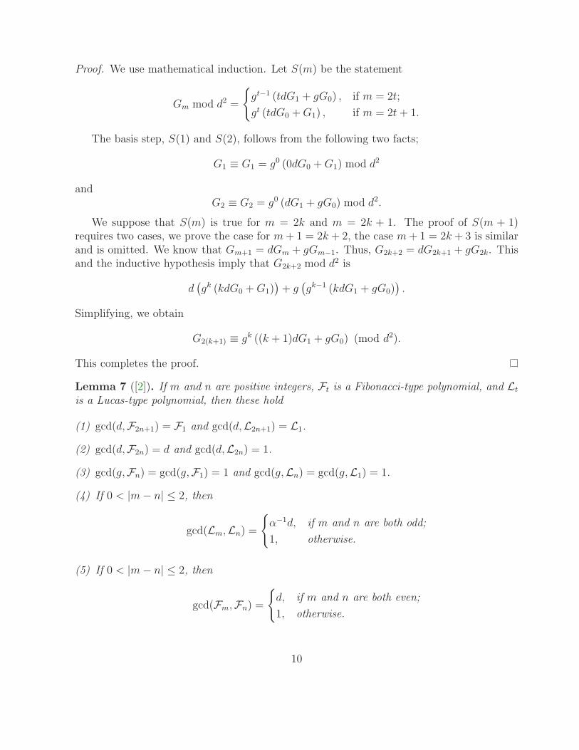
Proof. We use mathematical induction. Let S(m) be the statement

Gm mod d2 =

{

gt−1 (tdG1 + gG0) , if m = 2t;

gt (tdG0 +G1) , if m = 2t+ 1.

The basis step, S(1) and S(2), follows from the following two facts;

G1 ≡ G1 = g0 (0dG0 +G1) mod d2

andG2 ≡ G2 = g0 (dG1 + gG0) mod d2.

We suppose that S(m) is true for m = 2k and m = 2k + 1. The proof of S(m + 1)requires two cases, we prove the case for m+ 1 = 2k + 2, the case m+ 1 = 2k + 3 is similarand is omitted. We know that Gm+1 = dGm + gGm−1. Thus, G2k+2 = dG2k+1 + gG2k. Thisand the inductive hypothesis imply that G2k+2 mod d2 is

d(

gk (kdG0 +G1))

+ g(

gk−1 (kdG1 + gG0))

.

Simplifying, we obtain

G2(k+1) ≡ gk ((k + 1)dG1 + gG0) (mod d2).

This completes the proof.

Lemma 7 ([2]). If m and n are positive integers, Ft is a Fibonacci-type polynomial, and Lt

is a Lucas-type polynomial, then these hold

(1) gcd(d,F2n+1) = F1 and gcd(d,L2n+1) = L1.

(2) gcd(d,F2n) = d and gcd(d,L2n) = 1.

(3) gcd(g,Fn) = gcd(g,F1) = 1 and gcd(g,Ln) = gcd(g,L1) = 1.

(4) If 0 < |m− n| ≤ 2, then

gcd(Lm,Ln) =

{

α−1d, if m and n are both odd;

1, otherwise.

(5) If 0 < |m− n| ≤ 2, then

gcd(Fm,Fn) =

{

d, if m and n are both even;

1, otherwise.

10

Lemma 8. Suppose that Gk is either Fk or Lk for all k ≥ 0. Let Gm+1Gn−2, GmGn, andGm+2Gn−1 be the points in a triangle of the star of David and GmGn−1, Gm+2Gn−2, andGm+1Gn be the points in the second triangle of the star of David, with m and n positiveintegers where Gm Gn 6= G0 G0. If ∆t = gcd(Gt, Gt−2), then

gcd(GmGn−1, Gm+1Gn, Gm+2Gn−2) = gcd(Gn, Gm,∆m∆n)

andgcd(Gm+1Gn−2, GmGn, Gm+2Gn−1) = gcd(Gn−2, Gm+2,∆n∆m).

Proof. We prove that

gcd(GmGn−1, Gm+1Gn, Gm+2Gn−2) = gcd(Gn, Gm,∆m∆n).

From Lemma 5 Part (2) we have

gcd(GmGn−1, Gm+1Gn) = gcd(Gm, Gn) · gcd(Gn−1Gm+1).

Therefore,

gcd (GmGn−1, Gm+1Gn, Gm+2Gn−2) = gcd (gcd (GmGn−1, Gm+1Gn) , Gm+2Gn−2)

= gcd ((gcd(Gm, Gn) · gcd (Gn−1Gm+1)) , Gm+2Gn−2) .

From Lemma 7 Parts (4) and (5) we know that

gcd(Gm+2Gn−2, gcd(Gn−1, Gm+1)) = 1.

So,

gcd (GmGn−1, Gm+1Gn, Gm+2Gn−2) = gcd (gcd (Gm, Gn) , Gm+2, Gn−2)

= gcd (Gm, Gn, Gm+2Gn−2)

= gcd(Gm, gcd(Gn, Gm+2Gn−2)).

This and Lemma 5 imply that

gcd(GmGn−1, Gm+1Gn, Gm+2Gn−2) = gcd(Gm, gcd(Gn, Gm+2∆n))

= gcd(Gn, gcd(Gm, Gm+2∆n))

= gcd(Gn, gcd(Gm,∆m∆n))

= gcd(Gn, Gm,∆m∆n).

Similarly, we have gcd(Gm+1Gn−2, GmGn, Gm+2Gn−1) = gcd(Gn−2, Gm+2,∆n∆m).

11

3.1 Proof of the main theorems

Proof of Theorem 2. If in Lemma 8 we consider Gn = Fn, we have

gcd(FmFn−1,Fm+1Fn,Fm+2Fn−2) = gcd(Fn,Fm,∆m∆n) (6)

andgcd(Fm+1Fn−2,FmFn,Fm+2Fn−1) = gcd(Fn−2,Fm+2,∆m∆n), (7)

where ∆t = gcd(Ft,Ft−2).For this proof we consider three cases depending on the parity of m and n.

Case m and n are odd. From Lemma 7 Part (5) we have ∆m = ∆n = 1. This, (6), and(7) imply that

gcd(FmFn−1,Fm+1Fn,Fm+2Fn−2) = 1

andgcd(Fm+1Fn−2,FmFn,Fm+2Fn−1) = 1.

Case m and n have different parity. From Lemma 7 Part (5) we have ∆m∆n = d. This,(6), and (7) imply that

gcd(FmFn−1,Fm+1Fn,Fm+2Fn−2) = gcd(Fn,Fm, d)

andgcd(Fm+1Fn−2,FmFn,Fm+2Fn−1) = gcd(Fn−2,Fm+2, d).

From Lemma 7 Part (1) we have gcd(Fn,Fm, d) = 1 = gcd(Fn−2,Fm+2, d). Therefore,gcd(FmFn−1,Fm+1Fn,Fm+2Fn−2) = gcd(Fm+1Fn−2,FmFn,Fm+2Fn−1) = 1.

Case both m and n are even. Suppose that n = 2k1 and m = 2k2 for some k1, k2 ∈ N.So, from Lemma 7 Part (5) we have that ∆m = ∆n = d. Since F0 = 0 and F1 = 1, byProposition 6 we have

F2k1 ≡ k1gk1−1d (mod d2),

F2k2 ≡ k2gk2−1d (mod d2).

This and gcd(d, g) = 1 imply that

gcd(FmFn−1,Fm+1Fn,Fm+2Fn−2) = gcd(k1gk1−1d, k2g

k2−1d, d2) = d gcd(d, k1, k2).

Similarly we have that gcd(Fm+1Fn−2,FmFn,Fm+2Fn−1) = d gcd(d, k1 − 1, k2 + 1).Let β = (gcd(d, k1 − 1, k2 + 1)) / (gcd(d, k1, k2)). Therefore,

gcd(Fm+1Fn−2,FmFn,Fm+2Fn−1) = β gcd(FmFn−1,Fm+1Fn,Fm+2Fn−2).

We now prove Part (2). Factoring, we have that

gcd(Fm+1Fn−2,Fm+1Fn) · gcd(FmFn−1,Fm+2Fn−1)

is equal toFm+1Fn−1 · gcd(Fn−2,Fn) · gcd(Fm,Fm+2).

The conclusion follows using Lemma 7 Part (5).

12

Proof of Theorem 3. In Lemma 8 if we take Gn = Ln, we have

gcd(LmLn−1,Lm+1Ln,Lm+2Ln−2) = gcd(Ln,Lm,∆m∆n) (8)

andgcd(Lm+1Ln−2,LmLn,Lm+2Ln−1) = gcd(Ln−2,Lm+2,∆n∆m),

where ∆t = gcd(Lt,Lt−2). If m and n are not both odd, then the proof follows in a similarway as in the proof of Theorem 2.

Suppose that both m and n are odd, that is n = 2k1 + 1 and m = 2k2 + 1 where k1, k2are non-negative integers. Therefore, by Lemma 7 Part (4) we know that ∆m = ∆n = L1.Since L1|d, by Proposition 6 we have

Ln ≡ ngk1L1 (mod L21)

andLm ≡ mgk2L1 (mod L2

1).

This and (8) imply that

gcd(LmLn−1,Lm+1Ln,Lm+2Ln−2) = gcd(ngk1L1,mgk2L1, (L1)2).

This and gcd(d, g) = 1 imply that gcd(LmLn−1,Lm+1Ln,Lm+2Ln−2) = L1 gcd(n,m,L1).Similarly we can prove that

gcd(Lm+1Ln−2,LmLn,Lm+2Ln−1) = L1 gcd(L1, n− 2,m+ 2).

Let β′ = (gcd(L1, n− 2,m+ 2)) / (gcd(L1, n,m)). Then,

gcd(Lm+1Ln−2,LmLn,Lm+2Ln−1) = β′ gcd(LmLn−1,Lm+1Ln,Lm+2Ln−2).

We now prove Part (2). Factoring, we have that

gcd(Lm+1Ln−2,Lm+1Ln) gcd(LmLn−1,Lm+2Ln−1)

is equal toLm+1Ln−1 gcd(Ln−2,Ln) gcd(Lm,Lm+2).

The conclusion follows using Lemma 7 Part (4).

3.2 Corollaries of the main theorem

Theorems 2, 3, and 4 are also true for the star of David with a vertical configuration asdepicted in Figure 3 (with similar proofs). The following corollaries are a formalization ofsome results that are in the proofs of Theorems 2 and 3. For the following three corollarieswe suppose that the points are as given in Theorems 2 and 3 and Figure 2.

13

Figure 3: Vertical star of David.

Corollary 9. Let Gt be one of the following polynomials: Fibonacci, Lucas, Jacobsthal,Jacobsthal-Lucas, Chebyshev first kind polynomials, Pell-Lucas, and both Morgan-Voyce poly-nomials, for every t ∈ N. If Gm+1Gn−2, GmGn, and Gm+2Gn−1 are the points in a triangleof the star of David and GmGn−1, Gm+2Gn−2, and Gm+1Gn are the points in the secondtriangle of the star of David, then

gcd(Gm+1Gn−2, GmGn, Gm+2Gn−1) = gcd(GmGn−1, Gm+2Gn−2, Gm+1Gn).

Corollary 10. Suppose that Fm+1Fn−2, FmFn, and Fm+2Fn−1 are the points in a triangle ofthe star of David and FmFn−1, Fm+2Fn−2, and Fm+1Fn are the points in the second triangleof the star of David. If n = 2k1 and m = 2k2 where k1, k2 ∈ N, then the these hold

(1) if n ≥ 0 and Fn is a Pell polynomial or a Chebyshev polynomial of the second kind withk1k2 6≡ 0 (mod 4) and k1 6≡ k2 (mod 2), then

gcd(Fm+1Fn−2,FmFn,Fm+2Fn−1) = gcd(FmFn−1,Fm+2Fn−2,Fm+1Fn).

(2) If n ≥ 0 and Fn is a Fermat polynomial with k1k2 6≡ 0 (mod 9) and k1 6≡ 2k2 (mod 3),then

gcd(Fm+1Fn−2,FmFn,Fm+2Fn−1) = gcd(FmFn−1,Fm+2Fn−2,Fm+1Fn).

Corollary 11. Suppose that Lm+1Ln−2, LmLn, and Lm+2Ln−1 are the points in a triangleof the star of David and LmLn−1, Lm+2Ln−2, and Lm+1Ln are the points in the secondtriangle of the star of David. If m,n ≥ 0, Lt is a Fermat-Lucas polynomial for t ≥ 0, andLmLn 6= L0L0, then

gcd(Lm+1Ln−2,LmLn,Lm+2Ln−1) = gcd(LmLn−1,Lm+2Ln−2,Lm+1Ln).

4 The geometry of some identities

The aim of this section is to give geometric interpretations of some polynomial identitiesthat are known for the Fibonacci numbers. The novelty of this section is that we extend

14

some well-known numerical identities to {Fk} and to {Lk} sequences and provide geometricproofs for these identities instead of the classical mathematical induction proofs.

Hosoya-type triangles (polynomial and numeric) are good tools to discover, prove, orrepresent theorems geometrically. Some properties that have been found and proved alge-braically are easy to understand when interpreted geometrically using these triangles.

4.1 Identities in the Hosoya polynomial triangle

Lemma 12. If i, j, k, and r are nonnegative integers with k + j ≤ r, then in the Hosoyapolynomial triangle this holds

H(r + 2i, k + j + i)−H(r + 2i, k + i) = (−1)ig(H(r, k + j)−H(r, k)).

The proof of the Lemma 12 follows using induction and the rectangle property whichstates that H(n,m) = dH(n− 1,m) + gH(n− 2,m) (see Figure 4).

H(r,k+j)H(r,k)

H(r+2i,k+i) H(r+2i,k+j+i)

2i R

ows

j columns

Figure 4: Property of Rectangle.

It is well known that the Catalan identity is a generalization of the Cassini identity.Johnson [12], gives another numerical generalization of the Cassini and Catalan identities,called the Johnson identity. It states that for the Fibonacci number sequence {Fn},

FaFb − FcFd = (−1)r (Fa−rFb−r − Fc−rFd−r)

where a, b, c, d, and r are arbitrary integers with a+ b = c+ d.The example in Figure 5 gives a geometric representation of the numeric identities (the

same representation holds for polynomials). To represent the Cassini identity we take two

15

consecutive points in the Hosoya triangle along a horizontal line such that one point islocated in the central column of the triangle, see Figure 5. We then pick two other arbitraryconsecutive points P1 and P2 such that they form a vertical rectangle along with the firstpair of points. The subtraction of the horizontal points P1 and P2 gives ±1. Since the entriesof the triangle are products of Fibonacci numbers, we obtain the Cassini identity.

The second example in Figure 5 represents the Catalan identity. In this case we take anytwo horizontal points Q1 and Q2 where Q1 is located (arbitrarily) in the central column ofthe triangle. We then pick other two arbitrary points P1 and P2 which form a rectangle withQ1 and Q2. The subtraction of the horizontal points P1 and P2 gives ±(Q1 −Q2). Since theentries of the triangle are products of Fibonacci numbers, we obtain the Catalan identity.Note that if we eliminate the condition that Q1 must be in the central column, we obtainthe Johnson identity.

1

1 1

2 1 2

3 2 2 3

5 3 4 3 5

8 5 6 6 5 8

13 8 10 9 10 8 13

21 13 16 15 15 16 13 21

34 21 26 24 25 24 26 21 34

55 34 42 39 40 40 39 42 34 55

89 55 68 63 65 64 65 63 68 55 89

144 89 110 102 105 104 104 105 102 110 89 144

233 144 178 165 170 168 169 168 170 165 178 144 233

377 233 288 267 275 272 273 273 272 275 267 288 233 377

610 377 466 432 445 440 442 441 442 440 445 432 466 377 610

987 610 754 699 720 712 715 714 714 715 712 720 699 754 610 987

1597 987 1220 1131 1165 1152 1157 1155 1156 1155 1157 1152 1165 1131 1220 987 1597

2584 1597 1974 1830 1885 1864 1872 1869 1870 1870 1869 1872 1864 1885 1830 1974 1597 2584

Catalan identity

Cassini identity

Figure 5: Cassini and Catalan identities in the Hosoya Triangle.

Theorem 13. Let a, b, c, d and t be nonnegative integers with min{a, b, c, d}−t non-negative.Suppose that Gk is either Fk or Lk for all k ≥ 0. If a+ b = c+ d, then

∣

∣

∣

∣

Ga Gc

Gd Gb

∣

∣

∣

∣

= (−1)tgt∣

∣

∣

∣

Ga−t Gc−t

Gd−t Gb−t

∣

∣

∣

∣

.

Proof. Let i, j, k, and r be nonnegative integers such that a = k + j + i, b = r + i− k − j,c = k + i, d = r + i− k, and t = i. Therefore, by Lemma 12 and Proposition 1 the equalityholds.

Theorem 13 is a generalization of Johnson identity [12] and Falcon and Plaza identity[1]. As a consequence of Theorem 13 we state Corollary 14 — this generalizes the Catalan

16

identity to Fk and Lk. If in Corollary 14 we take r = 1, then we obtain a generalization ofCassini identity.

Corollary 14 (Catalan identity). Suppose that m, r are non-negative integers. If Gk iseither Fk or Lk for all k ≥ 0, then

∣

∣

∣

∣

Gm Gm+r

Gm−r Gm

∣

∣

∣

∣

= (−1)m−rgm−r

∣

∣

∣

∣

Gr G2r

G0 Gr

∣

∣

∣

∣

.

Proof. The proof is straightforward when the appropriate values of m and r are substitutedin Theorem 13 (see Figure 5). If we evaluate both determinants in Theorem 13 we obtainfour summands that are four points in the Hosoya polynomial triangle. Note that these fourpoints are the vertices of a rectangle in the Hosoya triangle.

R3

R1

R2

R4

0

0

0

0

Figure 6: Geometric interpretation of Theorem 15.

We observe that if we have a Hosoya triangle where the entries are products of twopolynomial of {Fk}, then we can draw rectangles with two vertices in the central line (theperpendicular bisector) of the triangle and a third vertex on the edge of the triangle (seeFigure 6). For a fixed i ∈ N let Ri be a rectangle with the extra condition that the uppervertex points are multiplied by g, then Lemma 12 guarantees that the sum of the two topvertices of Ri is equal to the sum of the remaining vertices of Ri. Since the points in theedge of this triangle are equal to zero, one of the vertices of Ri is equal to zero. The othervertex in the same vertical line is a polynomial Fi multiplied by one. This geometry givesrise to Theorem 15.

For the next result we introduce the following function. We recall that g is as defined in(1).

I(n) =

{

g, if n is even;

1, if n is odd.

17

Theorem 15. If n and k are positive integers, then

2n+1∑

j=2

I(j)F2j =

n∑

j=1

F4j+1

and2n+1∑

j=2

(−1)j+1I2(j)F22j = d

n∑

j=1

F8j+2.

Proof. First of all we recall that F1 = 1. We prove the first identity.

2n+1∑

j=2

I(j)F2j =

n∑

j=1

(F22j+1 + gF2

2j) =n

∑

j=1

(F4j+1F1 + F0F4j)

=n

∑

j=1

F4j+1.

We now prove the second identity. Let S :=∑2n+1

j=2 (−1)j+1I2(j)F22j. Lemma 12 implies

that

S =n

∑

j=1

(F24j+2 − g2F2

4j)

=n

∑

j=1

((

F24j+2 + gF2

4j+1

)

− g(

F24j+1 + gF2

4j

))

.

Since F1 = 1, we have

S =n

∑

j=1

((

F8j+3 + gF8j+1F0

)

− g(

F8j+1 + gF8j−1F0

))

= F1

n∑

j=1

(

F8j+3 − gF8j+1

)

= d

n∑

j=1

F8j+2.

This completes the proof.

Corollary 16 provides a closed formula for special cases of Theorem 15. We use Figure7 to give a geometric interpretation of Corollary 16. For brevity we only give an algebraicproof of Part (1), the algebraic proof of Part (2) is similar, therefore it is omitted, and insteadwe provide a geometric proof of Part (2). This gives us the geometric behavior of a zigzagpattern of points. Thus, Corollary 16 Part (2) states that the sum of all points that are inthe intersection of a finite zigzag configuration and the central line of the triangle is the lastpoint of the zigzag configuration (see Figure 7).

18

Corollary 16. Suppose that g is as defined in (1). Then these hold

(1)n

∑

j=1

g2n−jF4j−3 =F2n−1F2n

d.

(2) If (in particular) the sequence {Fk} satisfies that g = 1, then

2n−1∑

j=1

F2j =

F2n−1F2n

d.

Figure 7: Geometric interpretation of Corollary 16.

Proof. Since H(2n, n) = F2n, we have that gnH(1, 1) +

∑n

j=1 dgn−jF2

j is equal to

n∑

j=1

dgn−jH(2j, j) = gn−1(gH(1, 1) + dH(2, 1)) +n

∑

j=2

dgn−jF2j

= gn−1H(3, 1) + dgn−2H(4, 2) +n

∑

j=3

dgn−jF2j

= gn−2H(5, 3) +n

∑

j=3

dgn−jF2j

= gn−2F3F2 +n

∑

j=3

dgn−jF2j .

19

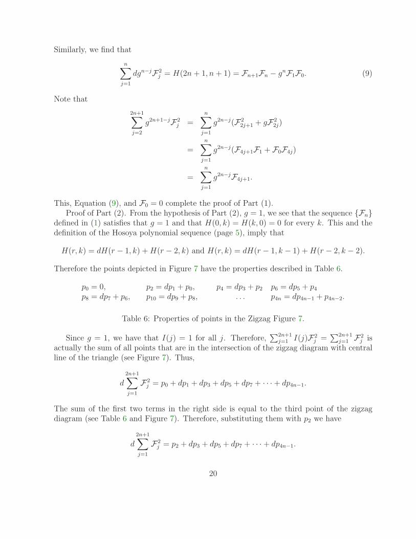
Similarly, we find that

n∑

j=1

dgn−jF2j = H(2n+ 1, n+ 1) = Fn+1Fn − gnF1F0. (9)

Note that

2n+1∑

j=2

g2n+1−jF2j =

n∑

j=1

g2n−j(F22j+1 + gF2

2j)

=n

∑

j=1

g2n−j(F4j+1F1 + F0F4j)

=n

∑

j=1

g2n−jF4j+1.

This, Equation (9), and F0 = 0 complete the proof of Part (1).Proof of Part (2). From the hypothesis of Part (2), g = 1, we see that the sequence {Fn}

defined in (1) satisfies that g = 1 and that H(0, k) = H(k, 0) = 0 for every k. This and thedefinition of the Hosoya polynomial sequence (page 5), imply that

H(r, k) = dH(r − 1, k) +H(r − 2, k) and H(r, k) = dH(r − 1, k − 1) +H(r − 2, k − 2).

Therefore the points depicted in Figure 7 have the properties described in Table 6.

p0 = 0, p2 = dp1 + p0, p4 = dp3 + p2 p6 = dp5 + p4p8 = dp7 + p6, p10 = dp9 + p8, . . . p4n = dp4n−1 + p4n−2.

Table 6: Properties of points in the Zigzag Figure 7.

Since g = 1, we have that I(j) = 1 for all j. Therefore,∑2n+1

j=1 I(j)F2j =

∑2n+1j=1 F2

j isactually the sum of all points that are in the intersection of the zigzag diagram with centralline of the triangle (see Figure 7). Thus,

d

2n+1∑

j=1

F2j = p0 + dp1 + dp3 + dp5 + dp7 + · · ·+ dp4n−1.

The sum of the first two terms in the right side is equal to the third point of the zigzagdiagram (see Table 6 and Figure 7). Therefore, substituting them with p2 we have

d

2n+1∑

j=1

F2j = p2 + dp3 + dp5 + dp7 + · · ·+ dp4n−1.

20

Now the sum of the first two terms of the right side of the previous equation is equal to thefifth point, p4, of the zigzag diagram (see Table 6 and Figure 7). Therefore, substitutingthem with p4 we have

d2n+1∑

j=1

F2j = p4 + dp5 + dp7 + · · ·+ dp4n−1.

Similarly, we substitute p4 + dp5 with the seventh point of the zigzag diagram. Thus,

d

2n+1∑

j=1

F2j = p6 + dp7 + · · ·+ dp4n−1.

Continuing this process, systematically substituting the terms, we obtain

d2n+1∑

j=1

F2j = p4n = F2n−1F2n.

This completes the geometric proof of Part (2).

4.2 Integration in the Hosoya triangle

We now discuss some examples on how the geometry of the triangle can be used to representidentities. The examples given in the following discussion are only for the case in which theHosoya triangle (denoted by HF ) has products of Fibonacci polynomials as entries. Withthis triangle in mind we introduce a notation that will be used in following examples. Wedefine an n-initial triangle as the finite triangular arrangement formed by the first n-rows ofHF with non-zero entries. Note that the initial triangle is the equilateral sub-triangle of theHosoya triangle as in Table 3 on page 6 without the entries containing the factor G0. Forinstance, Table 5 on page 7 represents the 5-initial triangle of HF .

If F ′n(x) represents the derivative of the Fibonacci polynomial Fn(x), then F ′

n(x) =∑n−1

k=1 Fk(x)Fn−k(x) (see [1, 14]). The geometric representation of this property in an n-initial triangle is as follows: the derivative of the first entry of the last row of a givenn-initial triangle is equal to the sum of all points of the penultimate row of this triangle (seeTable 5 on page 7). We have observed that this property implies that the integral of allpoints of the first n− 1 rows of a given n-initial triangle is equal to the sum of all points ofone edge of this triangle, where the constant of integration is ⌈n/2⌉. This result is statedformally in Proposition 17. Similar results can be obtained using Table 7.

Proposition 17. Let n be a positive number, then

(1)

H(n, 1) =n−1∑

k=1

∫

H(n− 1, k).

21

Equivalently,

Fn(x) =n−1∑

k=1

∫

Fk(x)Fn−k(x),

where the constant of integration is C = 1 if n is odd and zero otherwise.

(2)

H(n+ 1, 1) +H(n, 1)− 1 = xn

∑

r=1

r−1∑

k=1

∫

H(r − 1, k).

Equivalently,

Fn+1(x) + Fn(x)− 1 = xn

∑

r=1

r−1∑

k=1

∫

Fk(x)Fr−k(x),

where the constant of integration is C = ⌈n/2⌉.

Proof. The proof of Part (1) is straightforward using the geometric interpretation of F ′n(x).

We prove Part (2). From Part (1) and from the geometry of the (n−1)-initial triangle wehave

∑n

r=1 H(k, 1) =∑n−1

r=1

∑r−1k=1

∫

H(r − 1, k). From Koshy [14, Theorem 37.1] we knowthat Fn+1(x)+Fn(x)−1 = x

∑n

i=1 Fi(x). This and the fact that H(t, 1) = Ft(x) for all t ≥ 1completes the proof.

Derivative

F ′n(x) =

∑n−1k=1 Fk(x)Fn−k(x)

P ′n(x) = 2

∑n−1k=1 Pk(x)Pn−k(x)

Φ′n(x) = 3

∑n−1k=1 Φk(x)Φn−k(x)

U ′n(x) = 2

∑n−1k=1 Pk(x)Pn−k(x)

B′n(x) =

∑n−1k=1 Bk(x)Bn−k(x)

Table 7: Derivatives of Fibonacci-type polynomials.

5 Appendix. Numerical types of Hosoya triangle

In this section we study some connections of the Hosoya polynomial triangles with somenumeric sequences that may be found in [20]. We show that when we evaluate the entries

22

of a Hosoya polynomial triangle at x = 1 they give a triangle that is in http://oeis.org/.The first Hosoya triangle is the classic Hosoya triangle formerly called the Fibonacci triangle.

We now introduce some notation that is used in Table 8. Recall that HF is the Hosoyatriangle with products of Fibonacci polynomials as entries. Similarly we define the notationfor the Hosoya polynomial triangle of the other types — Chebyshev polynomials, Morgan-Voyce polynomials, Lucas polynomials, Pell polynomials, Fermat polynomials, Jacobsthalpolynomials. The star of David property holds obviously for all these numeric triangles.

Triangle type Notation Entries SloaneFibonacci HF (1) Fk(1)Fr−k(1) A058071Lucas HD(1) Dk(1)Dr−k(1) A284115Pell HP (1) Pk(1)Pr−k(1) A284127Pell-Lucas HQ(1) Qk(1)Qr−k(1) A284126Fermat HΦ(1) Φk(1)Φr−k(1) A143088Fermat-Lucas Hϑ(1) ϑk(1)ϑr−k(1) A284128Jacobsthal HJ(1) Jk(1)Jr−k(1) A284130Jacobsthal-Lucas Hj(1) jk(1)jr−k(1) A284129Morgan-Voyce HB(1) Bk(1)Br−k(1) A284131Morgan-Voyce HC(1) Ck(1)Cr−k(1) A141678

Table 8: Numerical Hosoya triangles present in Sloane [20].

We also observe some curious numerical patterns when we compute the gcd of the co-efficients of polynomials discussed in this paper. In particular, the gcd of the coefficientsof Φn(x), the nth Fermat polynomial, is 3an where an is the nth element of A168570. Thegcd of the coefficients of ϑn(x), the nth Fermat-Lucas polynomial, is 3an where an is thenth element of A284413. We also found that the gcd of the coefficients of the P2n(x), the2nth Pell polynomial, is 2an where an is the nth element of A001511. Finally, the gcd of thecoefficients of the Un(x), the nth Chebyshev polynomial of second kind, is 2an where an isthe nth element of A007814.

6 Acknowledgment

The first and last authors were partially supported by The Citadel Foundation. The authorsare grateful to an anonymous referee for the extensive comments and suggestions that helpedto improve the presentation of this paper.

References

[1] S. Falcon and A. Plaza, On k-Fibonacci sequences and polynomials and their derivatives,Chaos Solitons Fractals 39 (2009), 1005–1019.

23

[2] R. Florez, R. Higuita, and A. Mukherjee, Characterization of the strong divisibilityproperty for generalized Fibonacci polynomials, Integers 18 (2018), Paper No. A14.

[3] R. Florez, R. Higuita, and A. Mukherjee, Alternating sums in the Hosoya polynomialtriangle, J. Integer Seq. 17 (2014), Article 14.9.5.

[4] R. Florez, R. Higuita, and L. Junes, 9-modularity and GCD properties of generalizedFibonacci numbers, Integers 14 (2014), Paper No. A55.

[5] R. Florez, R. Higuita, and L. Junes, GCD property of the generalized star of David inthe generalized Hosoya triangle, J. Integer Seq. 17 (2014), Article 14.3.6.

[6] R. Florez and L. Junes, GCD properties in Hosoya’s triangle, Fibonacci Quart. 50

(2012), 163–174.

[7] A. P. Hillman and V. E. Hoggatt, Jr. A proof of Gould’s Pascal hexagon conjecture,Fibonacci Quart. 6 (1972), 565–568, 598.

[8] V. E. Hoggatt, Jr., and W. Hansell, The hidden hexagon squares, Fibonacci Quart. 9(1971), 120, 133.

[9] A. F. Horadam and J. M. Mahon, Pell and Pell-Lucas polynomials, Fibonacci Quart.23 (1985), 7–20.

[10] A. F. Horadam, Chebyshev and Fermat polynomials for diagonal functions, FibonacciQuart. 17 (1979), 328–333.

[11] H. Hosoya, Fibonacci triangle, Fibonacci Quart. 14 (1976), 173–178.

[12] R. C. Johnson, Fibonacci numbers and matrices, preprint available athttp://maths.dur.ac.uk/~dma0rcj/PED/fib.pdf.

[13] T. Koshy, Gibonomial coefficients with interesting byproducts, Fibonacci Quart. 53

(2015), 340–348.

[14] T. Koshy, Fibonacci and Lucas Numbers with Applications, Wiley, 2001.

[15] T. Koshy, Fibonacci and Lucas Numbers with Applications, Vol. 2, preprint.

[16] T. Koshy, Triangular Arrays with Applications, Oxford University Press, 2011.

[17] E. Korntved, Extensions to the GCD star of David theorem, Fibonacci Quart. 32 (1994),160–166.

[18] C. Long, W. Schulz, and S. Ando, An extension of the GCD Star of David theorem,Fibonacci Quart. 45 (2007), 194–201.

24

[19] B. Sagan and C. D. Savage, Combinatorial interpretations of binomial coefficient ana-logues related to Lucas sequences, Integers 10 (2010), 697–703.

[20] N. J. A. Sloane, The On-Line Encyclopedia of Integer Sequences, http://oeis.org/.

[21] Y. Sun, The star of David rule, Linear Algebra Appl. 429 (2008), 8–9, 1954–1961.

2010 Mathematics Subject Classification: Primary 11B39; Secondary 11B83.Keywords: Hosoya triangle, Gibonomial triangle, Fibonacci polynomial, Chebyshev poly-nomial, Morgan-Voyce polynomial, Lucas polynomial, Pell polynomial, Fermat polynomial.

(Concerned with sequences A001511, A007814, A058071, A141678, A143088, A168570, A284115,A284126, A284127, A284128, A284129, A284130, A284131, and A284413.)

Received May 31 2017; revised versions received March 5 2018; March 20 2018; April 152018. Published in Journal of Integer Sequences, May 8 2018.

Return to Journal of Integer Sequences home page.

25