Embed Size (px)
Citation preview
THE STANDARD MODEL
Stephen West
Department of Physics,
Royal Holloway, University of London,
Egham, Surrey,
TW20 0EX.
NExT graduate school lectures 2010-2014.
1
Contents
1 Introduction, Conventions and the fermionic content of the SM 5
1.1 Books and papers . . . . . . . . . . . . . . . . . . . . . . . . . . . . . . . . . . . . . . . 5
1.2 Overview . . . . . . . . . . . . . . . . . . . . . . . . . . . . . . . . . . . . . . . . . . . . 6
1.3 Conventions . . . . . . . . . . . . . . . . . . . . . . . . . . . . . . . . . . . . . . . . . . 8
1.4 Lorentz Invariance . . . . . . . . . . . . . . . . . . . . . . . . . . . . . . . . . . . . . . 8
1.5 C, P and CP . . . . . . . . . . . . . . . . . . . . . . . . . . . . . . . . . . . . . . . . . 12
1.6 Fermionic Content of SM . . . . . . . . . . . . . . . . . . . . . . . . . . . . . . . . . . . 14
2 Abelian Gauge Symmetry 16
2.1 Gauge Transformations . . . . . . . . . . . . . . . . . . . . . . . . . . . . . . . . . . . . 16
2.2 Gauge Fixing . . . . . . . . . . . . . . . . . . . . . . . . . . . . . . . . . . . . . . . . . 18
2.3 Summary - QED Lagrangian . . . . . . . . . . . . . . . . . . . . . . . . . . . . . . . . . 20
3 Non-Abelian Gauge Theories 21
3.1 Non-Abelian gauge transformations . . . . . . . . . . . . . . . . . . . . . . . . . . . . . 21
3.2 Non-Abelian Gauge Fields . . . . . . . . . . . . . . . . . . . . . . . . . . . . . . . . . . 22
3.3 Gauge Fixing . . . . . . . . . . . . . . . . . . . . . . . . . . . . . . . . . . . . . . . . . 25
3.4 Summary: The Lagrangian for a General non-Abelian Gauge Theory . . . . . . . . . . 27
3.5 Feynman Rules . . . . . . . . . . . . . . . . . . . . . . . . . . . . . . . . . . . . . . . . 29
4 Quantum Chromodynamics 31
4.1 Colour and the Spin-Statistics Problem . . . . . . . . . . . . . . . . . . . . . . . . . . . 31
4.2 QCD . . . . . . . . . . . . . . . . . . . . . . . . . . . . . . . . . . . . . . . . . . . . . . 32
4.3 Running Coupling . . . . . . . . . . . . . . . . . . . . . . . . . . . . . . . . . . . . . . . 33
4.4 Quark (and Gluon) Confinement . . . . . . . . . . . . . . . . . . . . . . . . . . . . . . 36
4.5 θ− Parameter and Strong CP problem. . . . . . . . . . . . . . . . . . . . . . . . . . . . 38
2
4.6 Summary . . . . . . . . . . . . . . . . . . . . . . . . . . . . . . . . . . . . . . . . . . . 40
5 Spontaneous Symmetry Breaking 41
5.1 Massive gauge bosons and Renormalisability . . . . . . . . . . . . . . . . . . . . . . . . 41
5.2 Spontaneous Symmetry Breaking . . . . . . . . . . . . . . . . . . . . . . . . . . . . . . 42
5.3 Spontaneous Symmetry Breaking . . . . . . . . . . . . . . . . . . . . . . . . . . . . . . 44
5.4 Goldstone Bosons . . . . . . . . . . . . . . . . . . . . . . . . . . . . . . . . . . . . . . . 47
5.5 The Higgs Mechanism . . . . . . . . . . . . . . . . . . . . . . . . . . . . . . . . . . . . 47
5.6 Gauge Fixing . . . . . . . . . . . . . . . . . . . . . . . . . . . . . . . . . . . . . . . . . 50
5.7 Bit more on Renormalisability . . . . . . . . . . . . . . . . . . . . . . . . . . . . . . . . 54
5.8 Spontaneous Symmetry Breaking in a Non-Abelian Gauge Theory . . . . . . . . . . . . 56
6 Spontaneous Breaking of SU(2)L × U(1)Y → U(1)EM 58
6.1 More on renormalisability . . . . . . . . . . . . . . . . . . . . . . . . . . . . . . . . . . 61
6.2 Summary . . . . . . . . . . . . . . . . . . . . . . . . . . . . . . . . . . . . . . . . . . . 63
7 The Electroweak Model of Leptons 64
7.1 Left- and right- handed fermions . . . . . . . . . . . . . . . . . . . . . . . . . . . . . . . 64
7.2 Fermion masses - Yukawa couplings . . . . . . . . . . . . . . . . . . . . . . . . . . . . . 66
7.3 Weak Interactions of Leptons . . . . . . . . . . . . . . . . . . . . . . . . . . . . . . . . 67
7.4 Classifying the Free Parameters . . . . . . . . . . . . . . . . . . . . . . . . . . . . . . . 70
7.5 Summary . . . . . . . . . . . . . . . . . . . . . . . . . . . . . . . . . . . . . . . . . . . 70
8 Electroweak Interactions of Hadrons 72
8.1 One Generation of Quarks . . . . . . . . . . . . . . . . . . . . . . . . . . . . . . . . . . 72
8.2 Quark Masses . . . . . . . . . . . . . . . . . . . . . . . . . . . . . . . . . . . . . . . . . 73
8.3 Adding Another Generation . . . . . . . . . . . . . . . . . . . . . . . . . . . . . . . . . 74
8.4 The GIM Mechanism . . . . . . . . . . . . . . . . . . . . . . . . . . . . . . . . . . . . . 76
3
8.5 Adding a Third Generation . . . . . . . . . . . . . . . . . . . . . . . . . . . . . . . . . 78
8.6 Mass generation - a summary . . . . . . . . . . . . . . . . . . . . . . . . . . . . . . . . 80
8.7 CP Violation . . . . . . . . . . . . . . . . . . . . . . . . . . . . . . . . . . . . . . . . . 82
8.8 Summary . . . . . . . . . . . . . . . . . . . . . . . . . . . . . . . . . . . . . . . . . . . 86
9 Neutrinos and the MNS matrix 88
9.1 Dirac Neutrino masses and mixings . . . . . . . . . . . . . . . . . . . . . . . . . . . . . 88
9.2 Majorana Neutrinos and the see-saw mechanism . . . . . . . . . . . . . . . . . . . . . . 88
9.3 MNS matrix and Counting phases for Dirac and Majorana Neutrinos . . . . . . . . . . 91
10 Anomalies 94
10.1 Triangle diagrams . . . . . . . . . . . . . . . . . . . . . . . . . . . . . . . . . . . . . . . 97
10.2 Chiral Anomalies and Chiral Gauge Theories . . . . . . . . . . . . . . . . . . . . . . . . 101
10.3 Cancellation of anomalies in the Standard Model. . . . . . . . . . . . . . . . . . . . . . 107
11 Chiral Lagrangian approximation 111
11.1 Explicit Chiral Symmetry Breaking . . . . . . . . . . . . . . . . . . . . . . . . . . . . . 118
11.2 Electroweak Interactions . . . . . . . . . . . . . . . . . . . . . . . . . . . . . . . . . . . 120
4
1 Introduction, Conventions and the fermionic content of the
SM
1.1 Books and papers
• F Halzen and A. D. Martin, Quarks and Leptons, Wiley, 1984.
• M. E. Peskin and D V Schroeder An Introduction to Quantum Field Theory Addison Wesley
1995.
• I J R Aitchison and A J G Hey Gauge theories in particle physics 2nd edition Adam Hilger 1989.
• J D Bjorken and S D Drell Relativistic Quantum Mechanics McGraw-Hill 1964.
• F Mandl and G Shaw Quantum Field Theory Wiley 1984.
• P. Ramond, Journeys beyond the standard model, Perseus Books, 1999.
• D. Balin and A. Love, Introduction to Gauge Field Theory, 1986.
• Several reviews on Spires, e.g. Teubner, Langacker, Signer, Novaes, Evans.
• Also useful S. P. Martin, A Supersymmetry primer
5
1.2 Overview
• The Standard Model is a description of the strong (SU(3)c), weak (SU(2)L) and electromagnetic
(U(1)em) interactions in terms of “gauge theories”. A gauge theory is one that possesses invariance
under a set of “local transformations” i.e. transformations whose parameters are space-time
dependent.
• Electromagnetism is a gauge theory, associated with the group U(1)em.
In this case the gauge transformations are local complex phase transformations of the fields of
charged particles.
Gauge invariance necessitates the introduction of a massless vector (spin-1) particle, the photon,
whose exchange mediates the electromagnetic interactions.
• In the 1950’s Yang and Mills considered (as a purely mathematical exercise) extending gauge
invariance to include local non-Abelian (i.e. non-commuting) transformations such as SU(2).
In this case one needs a set of massless vector fields (three in the case of SU(2)), which were
formally called “Yang-Mills” fields, but are now known as “gauge bosons”.
• In order to apply such gauge theories to the weak interaction, considers particle transforming into
each other under the weak interactions. → Doublets of weak isospin.
(uL
dL
)and
(νL
eL
)
• For SU(2)L we have three gauge bosons interpreted as the W±− and Z− bosons, that mediate
weak interactions in the same way that the photon mediates electromagnetic interactions.
• However, weak interactions are known to be short ranged, mediated by very massive vector-bosons,
whereas Yang-Mills fields are required to be massless in order to preserve the gauge invariance.
Solved by ⇒ the “Higgs mechanism”.
• Prescription for breaking the gauge symmetry spontaneously.
• Start with a theory that possesses the required gauge invariance, but the physical quantum states
of the theory are not invariant under the gauge transformations.
• The breaking of the invariance arises in the quantisation of the theory, whereas the Lagrangian
only contains terms which are invariant.
6
• One of the consequences of this is that the gauge bosons acquire a mass and can thus be applied
to weak interactions.
• Spontaneous symmetry breaking and the Higgs mechanism has another extremely important con-
sequence. It leads to a renormalisable theory with massive vector bosons.
⇒ Theory is renormalisable
Infinities that arise in higher order calculations can be re-absorbed into the parameters of the
Lagrangian (as in the case of QED).
• If we had simply broken the gauge invariance explicitly by adding mass terms for the gauge bosons,
resulting theory would not be renormalisable
⇒ Could not therefore have been used to carry out perturbative calculations.
• Consequence of the Higgs mechanism is the existence of a scalar (spin-0) particle - the Higgs
boson.
• Remaining step is to apply the ideas of gauge theories to the strong interactions.
The gauge theory of strong interactions is called “Quantum ChromoDynamics” (QCD), associated
with the group SU(3)c.
Quarks possess an internal property called “colour” and the gauge transformations are local
transformations between quarks of different colours.
The gauge bosons of QCD are called “gluons” and they mediate the strong interactions.
• The union of QCD and the electroweak gauge theory, which describes the weak and electromag-
netic interactions is known as the Standard Model.
• It has eighteen fundamental parameters, most of which are associated with the masses of the
gauge bosons, the quarks and leptons, and the Higgs.
• Not all independent and, for example, the ratio of the W− and Z− boson masses are (correctly)
predicted by the model.
• Since the theory is renormalisable, perturbative calculations can be performed which predict cross-
sections and decay rates both for strongly and weakly interacting processes.
Predictions have met with considerable success when confronted with ever stringent experimental
data.
7
1.3 Conventions
• Natural units: ~ = 1, c = 1
⇒ energy, momentum, mass, inverse time, inverse length all have same dimensions.
• The metric convention is
gµν = diag(1,−1,−1,−1) (1.1)
• Space time coords and derivatives
xµ = (x0, xi) = (t, x); xµ = gµνxν = (t,−x),
∂µ =
(∂
∂t,∇); ∂µ =
(∂
∂t,−∇
).
• Lorentz invariant inner product of two vectors:
x2 = gµνxµxν = xµx
µ = t2 − x.x
1.4 Lorentz Invariance
• An arbitrary Lorentz transformation can be written as
xµ → x′µ = Λµνxν
• Lorentz transforms defined by invariance of x2 under Λ ∈Lorentz Group
gµνxµxν = gρσΛ
ρµx
µΛσνxν , ∀ x
⇒ gµν = gρσ(Λ)ρµ(Λ)
σν .
• Klein-Gordon field, φ(x), transforms as
φ(x) → φ′(x) = φ(Λ−1x)
• Transformation should leave KG equation invariant, clearly 12m2φ2(x) is invariant, what about
the derivatives
∂µφ(x) → ∂µφ(Λ−1x) =
∂
∂xµφ(Λ−1x) =
∂(Λ−1)νρxρ
dxµ∂
∂(Λ−1)νρxρφ(Λ−1x)
= (Λ−1)νµ∂
∂(Λ−1)νρxρφ(Λ−1x) = (Λ−1)νµ(∂νφ)(Λ
−1x).
8
• Transformation of the kinetic term in KG Lagrangian
(∂µφ)2 → gµν(∂µφ
′(x))(∂νφ′(x)) = gµν[(Λ−1)ρµ(∂ρφ)][(Λ
−1)σµ(∂σφ)](Λ−1x)
= gρσ(∂ρφ)(∂σφ)(Λ−1x) = (∂ρφ)
2(Λ−1x)
• Thus the whole Lagrangian transforms as a scalar
L → L(Λ−1x)
and with the action, S, being an integral over all space of the Lagrangian it is clear that the action
is invariant.
Now Dirac Fermions
• Need a representation for the Lorentz group for Dirac spinors
• General 4-d Lorentz transformation
Lµν = i(xµ∂ν − xν∂µ)
• The Lorentz algebra is given by
[Lµν , Lρσ] = i(gνρLµσ − gµρLνσ − gνσLµρ + gµσLνρ)
• We can write down a 4-d matrix representation of the Lorentz generators (as we have Dirac Spinors
in mind) defined as
Sµν =i
4[γµ, γν ]
where the γ matrices are written in the Weyl or Chiral representation as
γµ =
(0 σµ
σµ 0
)where σµ = (1, σ) and σµ = (1,−σ)
where
σ1 =
(0 1
1 0
)σ2 =
(0 −ii 0
)σ3 =
(1 0
0 −1
)
which satisfy
σiσj = δij + iǫijkσk.
9
• We can then write the spinor form of the Lorentz transformation as:
Λ 1
2
= exp
(− i
2ωµνS
µν
).
such that a Dirac fermion, ψ transforms as
ψ(x) → Λ 1
2
ψ(Λ−1x).
In addition it can be shown that the γ matrices transform as
Λ−11
2
γµΛ 1
2
= Λµνγν (1.2)
• Using this we can show that the Dirac equation is invariant under Lorentz transformations:
[iγµ∂µ −m]ψ →[iγµ(Λ−1)νµ∂ν −m
]Λ 1
2
ψ(Λ−1x)
= Λ 1
2
Λ−11
2
[iγµ(Λ−1)νµ∂ν −m
]Λ 1
2
ψ(Λ−1x)
= Λ 1
2
[iΛ−1
1
2
γµΛ 1
2
(Λ−1)νµ∂ν −m]ψ(Λ−1x) using 1.2
= Λ 1
2
[iΛµσγ
σ(Λ−1)νµ∂ν −m]ψ(Λ−1x)
= Λ 1
2
[iγµ∂µ −m]ψ(Λ−1x) = 0
• Now we need to find how to write the Lagrangian for the Dirac theory, this will involve Dirac
bilinears.
• One guess ψ†ψ however this transforms as
ψ†ψ → ψ†Λ†1
2
Λ 1
2
ψ
but Λ†1
2
6= Λ−11
2
and so ψ†ψ is not Lorentz invariant.
• Better guess is ψ ≡ ψ†γ0 under an infinitesimal Lorentz transformation
ψ → ψ†(1 +i
2ωµν(S
µν)†)γ0
• For µ 6= 0 and ν 6= 0, associated with rotations, (Sµν)† = Sµν and commutes with γ0
• For µ = 0 or ν = 0, associated with boosts, (Sµν)† = −Sµν and anti-commutes with γ0
• this means that
ψ → ψ†(1 +i
2ωµν(S
µν))γ0
∴ ψ → ψΛ−11
2
10
• Consequently ψψ is a Lorentz invariant and the Dirac Lagrangian is
LDirac = ψ(iγµ∂µ −m)ψ.
Weyl and Majoran Spinors
• Much of the standard model (and MSSM) is written in terms of Weyl spinors. Weyl spinners are
two-component complex anticommuting objects. We can write a Dirac spinner in terms of two
Weyl spinners ξα and (χ†)α ≡ χ†α with two distinct indices α = 1, 2 and α = 1, 2:
ψD =
(ξα
χ†α
)
and
ψD = ψ†D
(0 1
1 0
)=(χα ξ†α
)
• Undotted indices are used for the first two components of a Dirac spinor
• Dotted indices are used for the last two components of a Dirac spinor
• ξ is called a “left-handed Weyl spinor” and χ† is a “right-handed Weyl Spinor”
• We can show this by using:
PL =1
2(1− γ5) and PR =
1
2(1 + γ5) with γ5 =
(−1 0
0 1
)
• We have:
PLΨD =
(ξα
0
), PRΨD =
(0
χ†α
)
• Hermitian conjugate of any left-handed Weyl spinner is a right-handed Weyl Spinner:
ψ†α ≡ (ψα)
† = (ψ†)α
and vice versa
(ψ†α)† = ψα
• Raise and lower indices using the antisymmetric symbol
ǫ12 = −ǫ21 = ǫ21 = −ǫ12 = 1, ǫ11 = ǫ22 = ǫ11 = ǫ22 = 0
with
ξα = ǫαβξβ, ξα = ǫαβξβ, χ†
α = ǫαβχ†β, χ†α = ǫαβχ†
β
11
• with
ǫαβǫβγ = ǫγβǫβα = δγα, ǫαβǫ
βγ = ǫγβǫβα = δγα
• The Dirac Lagrangian can then be written as:
L = ΨD(iγµ∂ −m)ΨD =
(χα ξ†α
)[( 0 iσµ∂µ
iσµ∂µ 0
)−(m 0
0 m
)](ξα
χ†α
)
= iχασµαα∂µχ†α + iξ†α(σ
µ)αα∂µξα −m(ξχ+ ξ†χ†)
= iχ†σµ∂µχ+ iξ†σµ∂µξ −m(ξχ+ ξ†χ†)
where the last step involves integration by parts and the identity χσµχ† = −χ†σµχ etc.
• A four component Majorana spinor can be obtained from the Dirac spinor by imposing the
condition χ = ξ such that,
ΨD =
(ξα
ξ†α
), ΨD =
(ξα ξ†α
)
• The Lagrangian for the Majorana spinor
LM =i
2ΨMγ
µ∂µΨM − 1
2MΨMΨM
= −iξ†σµ∂µξ −1
2M(ξξ + ξ†ξ†
)
• To efficiently move between theWeyl and Dirac notation we can use the chiral projection operators,
PL,R e.g.
ΨiPLΨj = χiξj and ΨiPRΨj = ξ†iχ†j
and
ΨiγµPLΨj = ξ†i σ
µξj and ψiγµPRΨj = χiσ
µχ†j = −χ†
j σµχi
1.5 C, P and CP
• How do these fields transform under C, P and CP
• Charge conjugation and Parity are defined by
C : ψ(t, x) → ψC(t, x) = CψT (t, x)
P : ψ(t, x) → ψP (t, x) = Pψ(t,−x)
with
C = iγ2γ0 and P = γ0
12
• Both C and P change the chirality: Consider purely LH state
PLψ(t, x) =
(ξ(t, x)
0
)
now act the parity operator on it
(PLψ(t, x))P = γ0
(ξ(t,−x)
0
)=
(0
ξ(t,−x)
)
we can see the final object is purely RH.
• Now for C:
(PLψ(t, x))C = iγ2γ0
(ξ(t, x)
0
)†
γ0
T
= iγ2γ0
(0
ξ†(t, x)
)
=
(0 iσ2
iσ2 0
)(0 1
1 0
)(0
ξ†(t, x)
)=
(0
iσ2ξ†(t, x)
)
the final result being RH.
• Charge conjugation and parity relate the LH and RH components. We will see later that LH and
RH states transform differently under the Weak force hence neither C nor P are good symmetries
when describing the weak force
• Combined application of both C and P leave a LH (RH) state LH (RH). Acting parity operator
on the above we have
(PLψ(t, x))CP =
[(PLψ(t, x))
C]P
=
(0
iσ2ξ†(t, x)
)P
= γ0
(0
iσ2ξ†(t,−x)
)=
(iσ2ξ†(t,−x)
0
)
which is still LH.
• CP is a better symmetry to use, but see later for CP -violation
• Majorana condition:
ψC = ψ
we can see this by taking the complex conjugate explicitly
ψCM = iγ2γ0ψTM = iγ2γ0
(ξα
ξ†α
)=
(−iσ2ξα−iσ2ξ†α
)=
(ξα
ξ†α
)= ψM
13
1.6 Fermionic Content of SM
The fermionic content (in terms of Weyl spinors) of the SM is as follows:
Qi =
(u
d
),
(c
s
),
(t
b
),
ui = u, c, t,
di = d, s, b,
Li =
(νe
e
),
(νµ
µ
),
(ντ
τ
),
ei = e, µ, τ .
“bars” are just labels not conjugates. Left handed states are written in doublets as they transform as
doublets under the SM gauge group SU(2), while RH states transform as singlets...more later.
• To form Dirac spinors: (e
e†
)
• Perhaps more used to writing things in terms of eL and eR, with identification e = eL and e = e†Rsuch that (
e
e†
)=
((eL)α
(eR)α
)
• A more transparent notation is thus:
QLi =
(uL
dL
),
(cL
sL
),
(tL
bL
),
uRi = uR, cR, tR,
dRi = dR, sR, bR,
LLi =
(νLe
eL
),
(νLµ
µL
),
(νLτ
τL
),
eRi = eR, µR, τR.
Example
• Dirac mass term for electrons
mD
2
((e†R)
α(eL)α + (e†L)α(eR)α)
14
using
e =
((eL)α
(eR)α
)e =
((e†R)
α (e†L)α
)
we can writemD
2(ePLe+ ePRe) =
mD
2ee
15
2 Abelian Gauge Symmetry
2.1 Gauge Transformations
• Consider the Lagrangian density for a free Dirac field ψ:
L = ψ(iγµ∂µ −m)ψ
• This Lagrangian density is invariant under the phase transformation of the fermion field and its
conjugate
ψ → eiωψ ψ → e−iωψ
• set of phases belong to the group U(1) and is abelian as
eiω1eiω2 = eiω2eiω1
• Infinitesimal form of this transformation
eiω ≈ 1 + iω +O(ω2)
under which the wavefunction changes by
δψ = iωψ
and the conjugate
δψ = −iωψ
under this lagrangian is invariant up to order ω2
• Now make the parameter ω depend on space-time
δψ(x) = iω(x)ψ(x) and δψ(x) = −iω(x)ψ(x)
• Such local (space-time) dependent transformations are called “gauge transformations”.
• The Lagrangian is now no longer invariant due to the derivative term giving the change in the
lagrangian of
ψ (iγµ∂µ −m)ψ → ψ′ (iγµ∂µ −m)ψ′ = (ψ − iω (x)) (iγµ∂µ −m) (ψ + iω (x)ψ)
= ψ (iγµ∂µ −m)ψ + ψ (γµ∂µω(x))ψ
⇒ δL = −ψ(x)γµ(∂µω(x))ψ(x)
16
• However, if we modify the Lagrangian by replacing ∂µ →Dµ = ∂µ + ieAµ
ψ (iγµ∂µ − eγµAµ −m)ψ = ψ (iγµ∂µ −m)ψ − eAµψγµψ
and demand that Aµ transforms according to:
Aµ → A′µ = Aµ −
1
e∂µω (x)
when
ψ → ψ′ = (ψ + iω (x)ψ),
then we will have restored local invariance!
• In other words, this is an invariance which only exists if the particles are not free! There is an
interaction term.
• Interpretation is: e is the electric charge of the fermion field and Aµ is the photon field.
• Dµ = ∂µ + ieAµ is the covariant derivative.
• It is easy to find the way the object Dµψ:
(Dµψ)′ = D′
µψ′ =(∂µ + ieA′
µ
)eiω(x)ψ = eiω(x)∂µψ+ i (∂µω (x)) eiω(x)+ ie
(Aµ −
1
e∂µω (x)
)eiω(x)ψ
⇒ D′µψ
′ = eiω(x) (∂µ + ieAµ)ψ = eiω(x)Dµψ
⇒ D′µψ
′ = eiω(x)Dµψ,
so Dµψ transforms like ψ. This means that ψDµψ is trivially invariant!
• To have a proper QFT we need Kinetic terms for the photon fields, must be gauge invariant.
Define field strength,
Fµν = ∂µAν − ∂νAµ
• Easy to see this is invariant but must be Lorentz invariant so we add to the Lagrangian
−1
4FµνF
µν
with the numerical factor included so that the equations of motion matches Maxwell’s equations.
• We can express this as
Fµν = − i
e[Dµ, Dν ] = − i
e[∂µ, ∂ν ] + [∂µ, Aν ] + [Aµ, ∂ν ] + ie[Aµ, Aν ] = ∂µAν − ∂νAµ
17
• Final Lagrangian density is
LQED = −1
4FµνF
µν + ψ (iγµ∂µ − eγµAµ −m)ψ = −1
4FµνF
µν + ψ (iγµDµ −m)ψ
with Dµ = ∂µ + ieAµ
• NOTE: no mass term for the photon such as M2AµAµ. If we add this and make a U(1) transfor-
mation
M2AµAµ → M2A′
µA′µ =M2AµA
µ − 2M2
eAµ∂µω
→ δL = −2M2
eAµ∂µω.
Thus gauge invariance requires a massless gauge boson.
2.2 Gauge Fixing
• In order to find the Feynman rule for the photon propagator (and to quantise the electromagnetic
field) we look for the parts of the action which are quadratic in the photon field.
• E.g. for some field φ(x) we take fourier transforms of the fields and identify the terms
Sφ =
∫d4pφ(−p)O(p)φ(p),
with the propagator for φ being
−iO−1(p).
• In the case of QED let us derive from the action in x-space, we have
S =
∫d4x
[−1
4(Fµν)
2
]=
∫d4x (∂µAν − ∂νAµ)(∂
µAν − ∂νAµ)
=
∫d4x Aµ(∂
2gµν − ∂µ∂ν)Aν
Now use Fourier transform for Aµ as
Aµ(x) =
∫d4p
(2π)4Aµ(p) e
ipx
S =
∫d4x
∫d4k
(2π)4d4p
(2π)4Aµ(p) e
ipx(∂2gµν − ∂µ∂ν) Aν(k) eikx
=
∫d4x
∫d4k
(2π)4d4p
(2π)4Aµ(p) e
i(p+k)x(−k2gµν − kµkν)Aν(k)
18
=
∫d4k
(2π)4d4p
(2π)4Aµ(p) δ
4(p+ k)(−k2gµν + kµkν)Aν(k)
=
∫d4p
(2π)4Aµ(p) (−p2gµν + pµpν)Aν(−p)
• However, this is not invertible, i.e.
(−p2gµν + pµpν)Dνρ(p) = iδµρ
has no solution as (−p2gµν + pµpν) is singular. Cannot find the propagator.
• Issue really comes down to the fact that we have gauge invariance. Troublesome modes are those
for which
Aµ =1
e∂µω(x)
that is those which are gauge equivalent to
Aµ(x) = 0.
Result is that the functional integral is badly defined...see QFT lectures
• Another interpretation is due to the fact that Aµ has four real components, introduced to maintain
gauge symmetry. However the physical photon has two polarisation states.
• This difficulty can be resolved by fixing the gauge (breaking the gauge symmetry) in the La-
grangian in such a way as to maintain the gauge symmetry in observables.
• Can solve this using method presented by Faddeev and Popov - needs functional integrals to do
properly but can be translated to adding to the Lagrangian density a gauge fixing term
−1
2
(∂.A)2
1− ξ
leading to
S =
∫d4p
(2π)4Aµ(p) (−p2gµν +
ξ
1− ξpµpν)Aν(−p)
(2.1)
using the relation (p2gµν − ξ
1− ξpµpν
)(gνρ −
ξpνpρp2
)= p2gµρ
we can now write the photon propagator as
−i(gµν − ξ
pµpνp2
)1
p2
19
• Special choice of ξ = 0 is known as the Feynman gauge. In this gauge the propagator is particularly
simple.
• We have to fix the gauge in order to be able to perform a calculation. Once we have computed a
physical measurable quantity, the dependence on the gauge cancels.
• Taking ξ = 0 is one choice, there are other special choices but the choice does not affect the result
of a calculation of a measurable quantity.
2.3 Summary - QED Lagrangian
Theory contains fermions with charge e, and a massless vector boson, the photon.
In Feynman Gauge
LQED = −1
4FµνF
µν + ψ (iγµDµ −m)ψ − 1
2(∂.A)2
with Dµ = ∂µ + ieAµ
Invariant under the transformations
Aµ → A′µ = Aµ −
1
e∂µω (x)
ψ(x) → ψ(x)′ = eiω(x)ψ(x) ψ(x) → ψ(x)′ = e−iω(x)ψ(x)
20
3 Non-Abelian Gauge Theories
3.1 Non-Abelian gauge transformations
• Extend “gauge” concept so that gauge bosons have self- interactions as observed for the gluons
of QCD, and the W±, Z of the electroweak sector.
• However, the gauge bosons will still be massless. (We will see how to give the W± and Z their
observed masses in the Higgs chapter.)
• Non-Abelian means different elements of the group do not commute with each other.
• Transformations act between a degenerate space of states (for example between u-d quarks states
where both have the same masses in isospin)
• Consider n free fermion fields ψ, arranged in a multiplet ψ
ψ =
ψ1
ψ2
.
.
ψn
• The Lagrangian density for a ψ is
L = ψi(iγµ∂µ −m)ψi, (3.1)
where the index i is summed from 1 to n. Eq.(3.1) is therefore shorthand for
L = ψ1(iγµ∂µ −m)ψ1 + ψ
2(iγµ∂µ −m)ψ2 + .... (3.2)
• The Lagrangian density is invariant under the global complex transformations in field (ψi) space:
ψ → ψ′ = Uψ ψ → ψ′ = ψU†
where U is an n× n unitary matrix
U†U = 1, det[U] = 1
• These matrices will form the group SU(n).
21
• In order to specify an SU(n) matrix we need n2 − 1 real parameters.
• An arbitrary SU(n) matrix can be written as
U = e−iΣn2
−1
a=1ωa
Ta ≡ e−iω
aT
a
• ωa are real parameters, and the Ta are the generators of the SU(n) group
• Generators are hermitian and traceless (can prove these facts by unitarity condition and determi-
nant condition respectively
• For SU(n) there are n2−1 generators Ta which are normalised, in the fundamental representation,
using the convention
tr(TaTb) =1
2δab
• Two such transformations do not commute.
(eiω
a1Ta) (
eiωb2Tb)
6=(eiω
b2Tb) (eiω
a1Ta)
.
• Specifically the Lie algebra of the SU(n) group is written in terms of commutators:
[Ta,Tb] = ifabcTc
where fabc are called structure functions of the SU(n) group and are totally antisymmetric.
3.2 Non-Abelian Gauge Fields
• Now consider local SU(n) transformations, as with abelian symmetries the lagrangian is no longer
invariant
L → L′ = ψU†(iγµ∂µ −m)Uψ = ψ(iγµ∂µ −m)ψ + iψU†γµ(∂µU)ψ
• In analogy with the abelian case we introduce the covariant derivative
Dµ = ∂µ + igAµ
where Aµ = TaAµ
• Covariant derivative contains n2 − 1 (spin 1) gauge bosons, Aaµ, one for each generator.
22
• The quantity Aµ transforms as
Aµ → A′µ = UAµU
† +i
g(∂µU)U† (3.3)
• sometimes useful to use infinitesimal form which can be found by the following, using U = e−iωaTa
,
A′µ = UAµU
† +i
g(∂µU)U† = e−iω
bTb
AaµTaeiω
bTb
+i
g(∂µe
−iωaTa
)eiωaTa
≈ (1− iωbTb)AaµTa(1 + iωbTb) +
i
g(∂µ(1− iωaTa))(1 + iωaTa)
≈ AaµTa − iωbTbAaµT
a + iAaµTaωbTb +
1
g(∂µω
a)Ta
≈ AaµTa + i[Ta,Tb]ωbAaµ +
1
g(∂µω
a)Ta
≈ AaµTa − fabcTcωbAaµ +
1
g(∂µω
a)Ta
• It is easy to check how Dµψ transforms:
Dµψ → (Dµψ)′ =
[∂µ + ig(UAµU
† +i
g(∂µU)U†
]Uψ (3.4)
= U∂µψ + igUAµψ − (∂µU)ψ + (∂µU)ψ
= U∂µψ + igUAµψ
= UDµψ
• Trivial to then check invariance of the lagrangian
• The kinetic term for the gauge bosons is again constructed from the field strengths F aµν which are
defined from the commutator of two covariant derivatives:
Fµν = − i
g[Dµ,Dν ] . (3.5)
where the matrix Fµν is given by
Fµν = TaF aµν ,
Fµν = − i
g[Dµ,Dν ] = (∂µ + igAµ)(∂ν + igAν)− (∂ν + igAν)(∂µ + igAµ)
= (∂µAν)− (∂νAµ) + ig(AµAν −AνAµ)
23
= (∂µAaν)T
a − (∂νAaµ)T
a + igAbµAcν(T
bTc −TcTb)
= [(∂µAaν)− (∂νA
aµ)]T
a + igAbµAcν [T
b,Tc]
=([(∂µA
aν)− (∂νA
aµ)]− gfabcAbµA
cν
)Ta
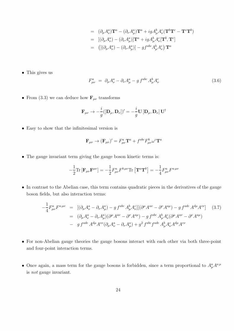
• This gives us
F aµν = ∂µA
aν − ∂νA
aµ − g fabcAbµA
cν (3.6)
• From (3.3) we can deduce how Fµν transforms
Fµν → − i
g([Dµ,Dν ])
′ = − i
gU [Dµ,Dν ]U
†
• Easy to show that the infinitesimal version is
Fµν → (Fµν)′ = F a
µνTa + fabcF b
µνωcTa
• The gauge invariant term giving the gauge boson kinetic terms is:
−1
2Tr [FµνF
µν ] = −1
2F aµνF
b µνTr[TaTb
]= −1
4F aµνF
aµν
• In contrast to the Abelian case, this term contains quadratic pieces in the derivatives of the gauge
boson fields, but also interaction terms:
−1
4F aµνF
aµν = [(∂µAaν − ∂νA
aµ)− g fabcAbµA
cν ][(∂
µAaν − ∂νAaµ)− g fadeAdµAeν ] (3.7)
= (∂µAaν − ∂νA
aµ)(∂
µAaν − ∂νAaµ)− g fabcAbµAcν(∂
µAaν − ∂νAaµ)
− g fadeAdµAeν(∂µAaν − ∂νA
aµ) + g2 fabcfadeAbµA
cνA
dµAeν
• For non-Abelian gauge theories the gauge bosons interact with each other via both three-point
and four-point interaction terms.
• Once again, a mass term for the gauge bosons is forbidden, since a term proportional to AaµAaµ
is not gauge invariant.
24
3.3 Gauge Fixing
• As with the abelian symmetries, we need to add a gauge fixing term in order to be able to derive
a propagator for the gauge bosons.
• In the Feynman gauge this means adding the term
−1
2(∂µAaµ)
2
to the Lagrangian density and the propagator (in momentum space) becomes
−i δabgµνp2.
• One unfortunate complication only needed for the purpose of performing higher loop calculations
with non-Abelian gauge theories.
• A consequence of gauge-fixing is that we need extra loop diagrams in higher order which are
mathematically equivalent to interacting scalar particles known as a “Faddeev-Popov ghost” for
each gauge field.
• These are not physical scalar particles and cannot appear as external legs on diagrams
1. They only occur inside loops.
2. They behave like fermions even though they are scalars (spin zero). This means that we need to
count a minus sign for each loop of Faddeev-Popov ghosts in any Feynman diagram.
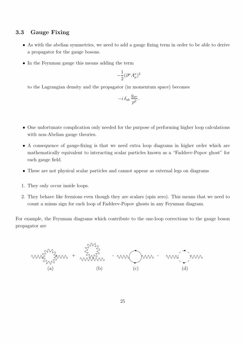
For example, the Feynman diagrams which contribute to the one-loop corrections to the gauge boson
propagator are
+ - -
(a) (b) (c) (d)
25

• (a) - three-point interaction between the gauge bosons
• (b)- four-point interaction between the gauge bosons
• (c) involves a loop of fermions,
• (d) extra diagram involving the Faddeev-Popov ghosts.
• Both (c) and (d) have a minus sign in front of them because both the fermions and Faddeev-Popov
ghosts obey Fermi statistics.
26
3.4 Summary: The Lagrangian for a General non-Abelian Gauge Theory
Consider a group gauge group, G of “dimension” N , whose N generators, Ta, obey the commutation
relations [Ta,Tb
]= ifabcTc, (3.8)
where fabc are called the “structure constants” of the group (they are antisymmetric in the indices
a, b, c).
• These matrices satisfy the Jacobi identity,
[TA,
[TB,TC
]]+[TB,
[TC ,TA
]]+[TC ,
[TA,TB
]]= 0 (3.9)
which means,
fADEfBCD + fBDEfCAD + fCDEfABD = 0. (3.10)
We can then define a da × da ,matrix,
(TC)AB ≡ −ifABC , (3.11)
which satisfy the Lie algebra.
• The matrices form a real representation in a da-dimensional vector space and is called the adjoint.
The dimension of this space is equal to the number of generators.
• The TrA matrices which represent the algebra in representation r satisfy a normalisation condition,
Tr(TrATr
B) = CrδAB. (3.12)
where Cr is the Dynkin index for the representation r.
• In addition if we multiply by δAB and sum over A and B, we have,
drC(r) = Crda (3.13)
where dr is the dimension of the representation and C(r) is the quadratic Casimir operator of the
representation r, defined byda∑
A
TrATr
B = C(r)I
where I is the dr × dr identity matrix.
• In Table 1, we summarise some properties of the fundamental and adjoint representations of
SU(N).
27
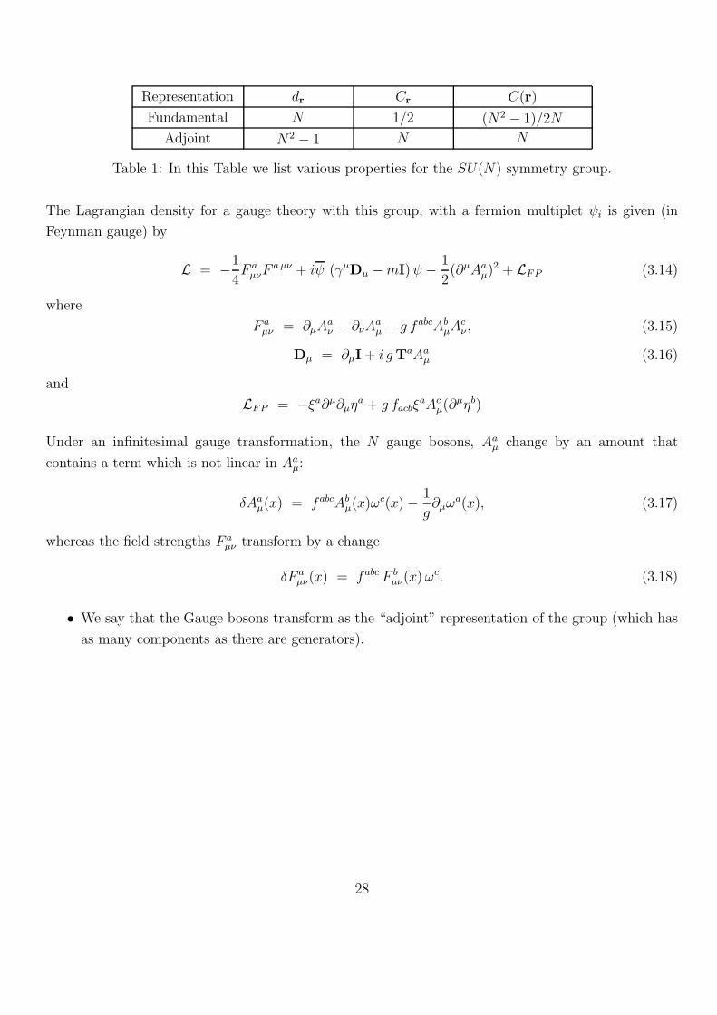
Representation dr Cr C(r)
Fundamental N 1/2 (N2 − 1)/2N
Adjoint N2 − 1 N N
Table 1: In this Table we list various properties for the SU(N) symmetry group.
The Lagrangian density for a gauge theory with this group, with a fermion multiplet ψi is given (in
Feynman gauge) by
L = −1
4F aµνF
aµν + iψ (γµDµ −mI)ψ − 1
2(∂µAaµ)
2 + LFP (3.14)
where
F aµν = ∂µA
aν − ∂νA
aµ − g fabcAbµA
cν , (3.15)
Dµ = ∂µI+ i gTaAaµ (3.16)
and
LFP = −ξa∂µ∂µηa + g facbξaAcµ(∂
µηb)
Under an infinitesimal gauge transformation, the N gauge bosons, Aaµ change by an amount that
contains a term which is not linear in Aaµ:
δAaµ(x) = fabcAbµ(x)ωc(x)− 1
g∂µω
a(x), (3.17)
whereas the field strengths F aµν transform by a change
δF aµν(x) = fabc F b
µν(x)ωc. (3.18)
• We say that the Gauge bosons transform as the “adjoint” representation of the group (which has
as many components as there are generators).
28
3.5 Feynman Rules
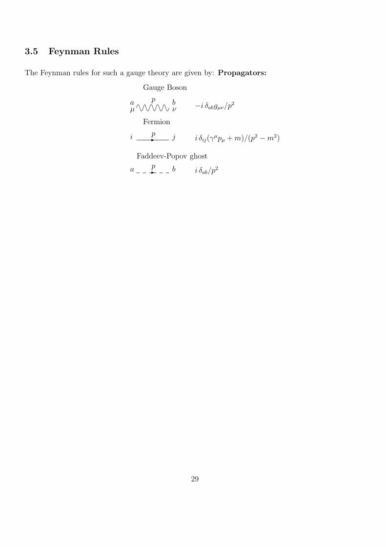
The Feynman rules for such a gauge theory are given by: Propagators:
Gauge Boson
−i δabgµν/p2pa
µbν
Fermion
i δij(γµpµ +m)/(p2 −m2)
pi j
Faddeev-Popov ghost
i δab/p2pa b
29
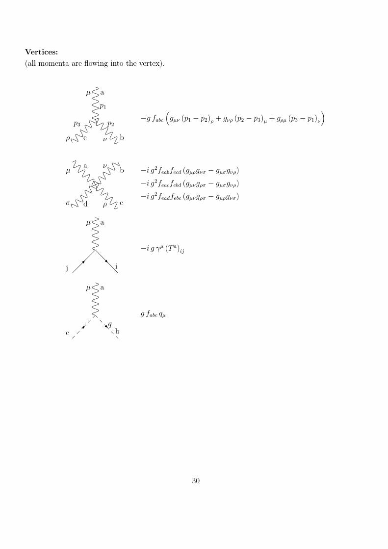
Vertices:
(all momenta are flowing into the vertex).
µ a
p1
ρ c
p3
ν b
p2−g fabc
(gµν (p1 − p2)ρ + gνρ (p2 − p3)µ + gρµ (p3 − p1)ν
)
−i g2feabfecd (gµρgνσ − gµσgνρ)
−i g2feacfebd (gµνgρσ − gµσgνρ)
−i g2feadfebc (gµνgρσ − gµρgνσ)
µa ν
b
σ d ρ c
µ a
j i
−i g γµ (T a)ij
µ a
c bq
g fabc qµ
30
4 Quantum Chromodynamics
4.1 Colour and the Spin-Statistics Problem
• Motivation for colour:
∆++
consists of uuu and has spin 3/2 and is in the l = 0 angular momentum state
wavefunction seems to be symmetric under exchange of quarks - exclusion principle says this
cannot be so
• Fermions should have a wavefunction which is antisymmetric under the interchange of the quantum
numbers of any two fermions.
• Solved by allowing quarks to also carry one of three “colours”
• As well as the flavour index, (f) a quark field carries a colour index, i, so we write a quark field
as qif , i = 1 · · ·3.
• It was further assumed that the strong interactions are invariant under colour SU(3) transforma-
tions.
• The quarks transform as a triplet representation of the group SU(3) which has eight generators.
• Furthermore it was assumed that all the observed hadrons are singlets of this new SU(3) group.
• Spin statistics problem is now solved
• Baryon consists of three quarks and a colour singlet state
• Colour part of the wavefunction is
|B > = ǫijk|qif1qjf2qkf3 >,
where f1, f2, f3 are the flavours of the three quarks that make up the baryon B and i, j, k are
the colours.
• Tensor ǫijk is totally antisymmetric under the interchange of any two indices, so that if the part of
the wavefunction of the baryon that does not depend on colour is symmetric, the total wavefunction
(including the colour part) is antisymmetric, as required by the spin-statistics theorem.
31
4.2 QCD
• QCD is where invariance under colour SU(3) transformations is promoted to an invariance under
local SU(3) (gauge) transformations.
• Quarks transform as triplets and anti-quarks transform as anti-triplets under SU(3)C
• a quark transforms as
q → q′ = ei2α .λ q
with eight finite real parameters (α = (α1, α2, ......, α8)) and λ stands for eight Hermitian 3× 3
matrices (the generators of SU(3)), λ = (λ1, ...., λ8),
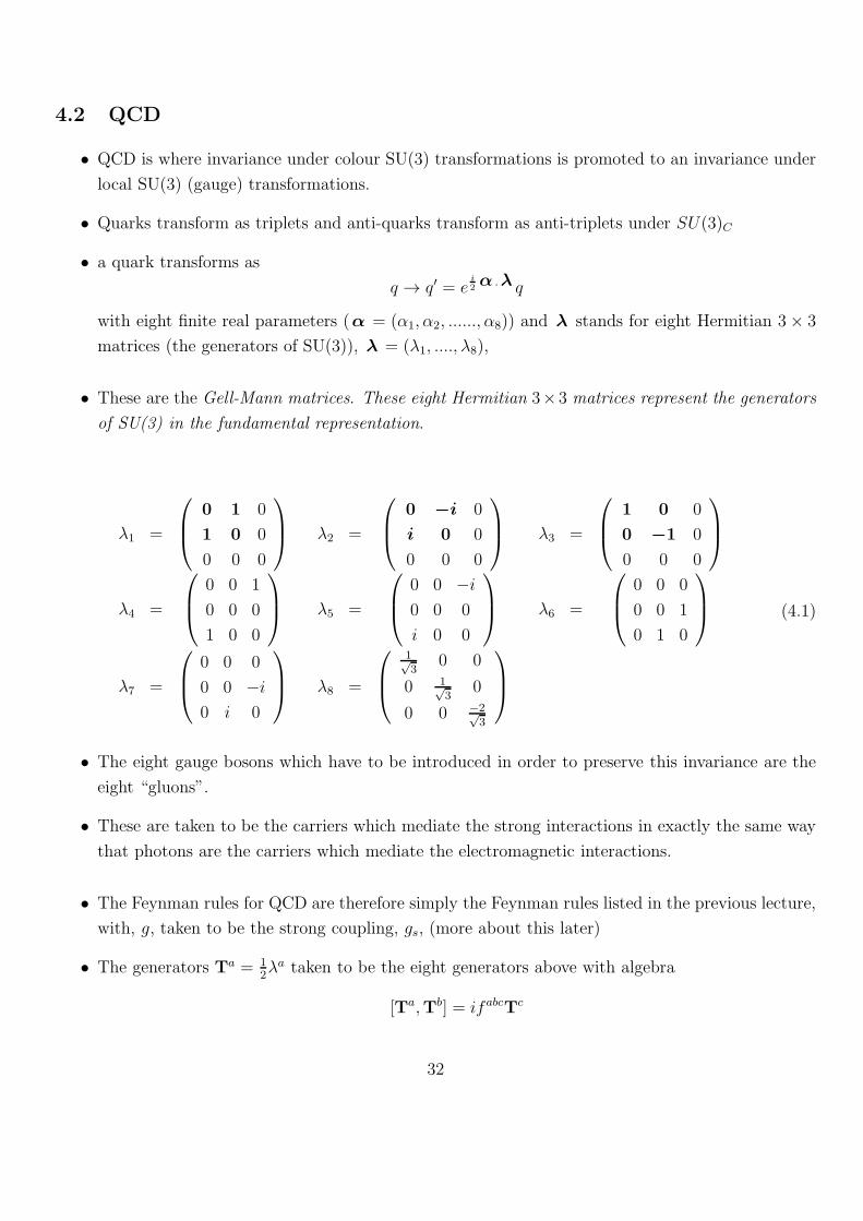
• These are the Gell-Mann matrices. These eight Hermitian 3×3 matrices represent the generators
of SU(3) in the fundamental representation.
λ1 =
0 1 0
1 0 0
0 0 0
λ2 =
0 −i 0
i 0 0
0 0 0
λ3 =
1 0 0
0 −1 0
0 0 0
λ4 =
0 0 1
0 0 0
1 0 0
λ5 =
0 0 −i0 0 0
i 0 0
λ6 =
0 0 0
0 0 1
0 1 0
λ7 =
0 0 0
0 0 −i0 i 0
λ8 =
1√3
0 0
0 1√3
0
0 0 −2√3
(4.1)
• The eight gauge bosons which have to be introduced in order to preserve this invariance are the
eight “gluons”.
• These are taken to be the carriers which mediate the strong interactions in exactly the same way
that photons are the carriers which mediate the electromagnetic interactions.
• The Feynman rules for QCD are therefore simply the Feynman rules listed in the previous lecture,
with, g, taken to be the strong coupling, gs, (more about this later)
• The generators Ta = 12λa taken to be the eight generators above with algebra
[Ta,Tb] = ifabcTc
32
with fabc, a, b, c, = 1 · · · 8 the structure constants of SU(3) with values
f 123 = 1
f 147 = −f 156 = f 246 = f 257 = f 345 = −f 367 =1
2
f 458 = f 678 =
√3
2
• To maintain gauge invariance we again exchange ∂µ → Dµ = ∂µ − igs2Aaµλ
a
Thus we now have a Quantum Field Theory which can be used to describe the strong interactions.
4.3 Running Coupling
• The coupling for the strong interactions is the QCD gauge coupling, gs. We usually work in terms
of αs defined as
αs =g2s4π.
• Since the interactions are strong, we would expect αs to be too large to perform reliable calcula-
tions in perturbation theory.
• On the other hand the Feynman rules are only useful within the context of perturbation theory.
• Difficulty resolved as “coupling constants” are not constant at all.
• The electromagnetic fine structure constant, α, only has the value 1/137 at energies which are
not large compared with the electron mass.
At higher energies it is larger than this.
• For example, at LEP energies it takes a value closer to 1/128.
• On the other hand, it turns out that for non-Abelian gauge theories the coupling decreases as the
energy increases.
• To see how in QCD, we note that when we perform higher order perturbative calculations there
are loop diagrams which dress the couplings.
• For example, the one-loop diagrams which dress the coupling between a quark and a gluon are:
33
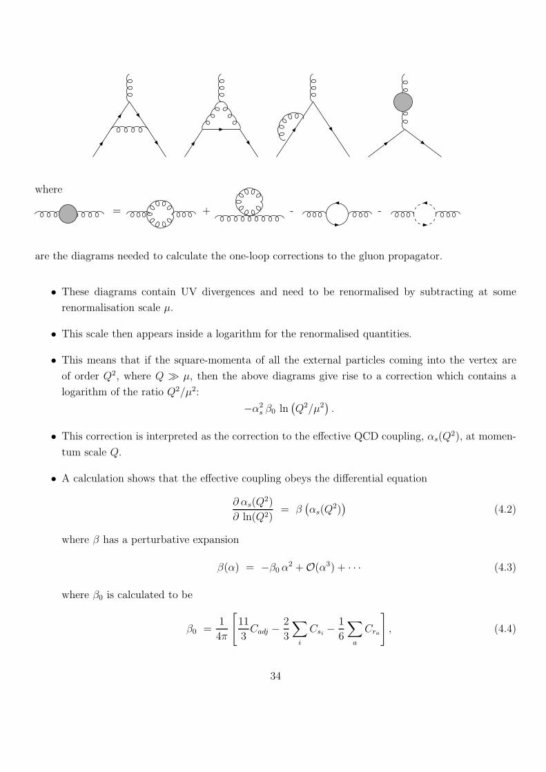
where
= + - -
are the diagrams needed to calculate the one-loop corrections to the gluon propagator.
• These diagrams contain UV divergences and need to be renormalised by subtracting at some
renormalisation scale µ.
• This scale then appears inside a logarithm for the renormalised quantities.
• This means that if the square-momenta of all the external particles coming into the vertex are
of order Q2, where Q ≫ µ, then the above diagrams give rise to a correction which contains a
logarithm of the ratio Q2/µ2:
−α2s β0 ln
(Q2/µ2
).
• This correction is interpreted as the correction to the effective QCD coupling, αs(Q2), at momen-
tum scale Q.
• A calculation shows that the effective coupling obeys the differential equation
∂ αs(Q2)
∂ ln(Q2)= β
(αs(Q
2))
(4.2)
where β has a perturbative expansion
β(α) = −β0 α2 +O(α3) + · · · (4.3)
where β0 is calculated to be
β0 =1
4π
[11
3Cadj −
2
3
∑
i
Csi −1
6
∑
a
Cra
], (4.4)
34
where where considering contributions from fields transforming as the adjoint, scalars transforming
with representation si and fermions transforming with representation ra. The Cs are the dynkin
indices for the particular representations, r, defined by
Tr[T ar Tbr ] = Crδ
ab (4.5)
• There are no scalars charged under QCD
• For the adjoint and fermions transforming under the fundamental and anti-fundamental we have
Tr[T aadjTbadj ] = Ncδ
ab, T r[T aFTbF ] =
1
2δab, T r[T aFT
bF ] =
1
2δab (4.6)
• So we get with Nc = 3
β0 =1
4π
[11
33− 2
3
[nf
1
2+ nf
1
2
]]=
[33− 2nf ]
12π
• nf is the number of active flavours, i.e. the number of flavours whose mass threshold is below the
momentum scale, Q.
• Solving this do it from the differential form we find
αs(Q2) =
αs(µ2)
1 + β0αs(µ2) ln Q2
µ2
Now we need a boundary value.
• This is taken to be the measured value of the coupling at the Z−boson mass (= 91 GeV), which
is measured to be
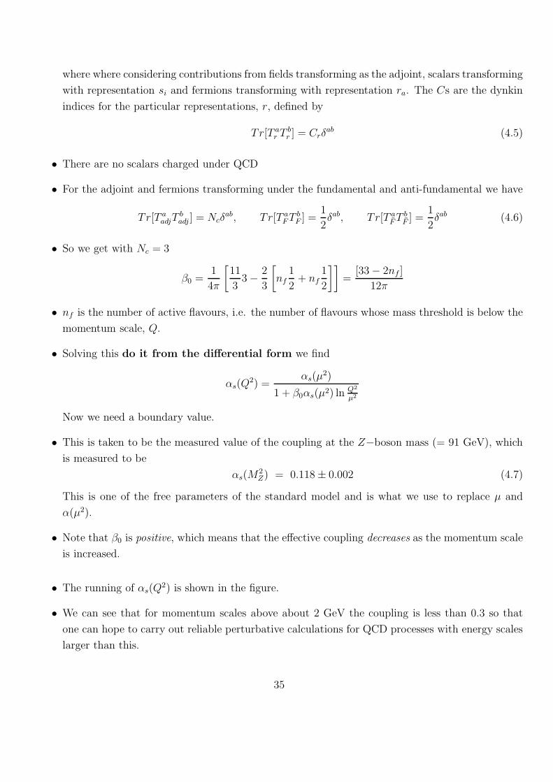
αs(M2Z) = 0.118± 0.002 (4.7)
This is one of the free parameters of the standard model and is what we use to replace µ and
α(µ2).
• Note that β0 is positive, which means that the effective coupling decreases as the momentum scale
is increased.
• The running of αs(Q2) is shown in the figure.
• We can see that for momentum scales above about 2 GeV the coupling is less than 0.3 so that
one can hope to carry out reliable perturbative calculations for QCD processes with energy scales
larger than this.
35
• Gauge invariance requires that the gauge coupling for the interaction between gluons must be
exactly the same as the gauge coupling for the interaction between quarks and gluons.
• The β−function could therefore have been calculated from the higher order corrections to the
three-gluon (or four-gluon) vertex
→ must yield the same result, despite the fact that it is calculated from a completely different set
of diagrams.
4.4 Quark (and Gluon) Confinement
• This argument can be inverted to provide an answer to the question ‘why have we never seen
quarks or gluons in a laboratory ? ’.
• Asymptotic freedom, which tells us that the effective coupling between quarks becomes
weaker as we go to short distances (this is equivalent to going to high energies) implies,
conversely, that effective couplings grow as we go to large distances.
36
• Therefore, the complicated system of gluon exchanges, which leads to the binding of quarks (and
antiquarks) inside hadrons, leads to a stronger and stronger binding as we attempt to pull the
quarks apart.
• This means that we can never isolate a quark (or a gluon) at large distances since we require more
and more energy to overcome the binding as the distance between the quarks grows.
• Only free particles which can be observed at macroscopic distances from each other are colour
singlets.
• Mechanism is known as “quark confinement”.
• Details are not fully understood.
At the level of non-perturbative field theory, lattice calculations have confirmed that the binding
energy grows as the distance between quarks increases.
• Thus we have two different pictures of the world.
• Short distances, or large energies, quarks and gluons are the appropriate degrees of freedom
to do calculations with.
They are what we consider interacting with each other.
e.g. We can perform calculations of the scattering cross-sections between quarks and gluons (called
the “hard cross-section”)
• This is because running coupling is sufficiently small so that we can rely on perturbation theory.
• However, on the other hand in experiments, we need to take into account the fact that these
quarks and gluons bind into colour singlet hadrons
→ only these colour singlet states that are observed.
• The mechanism for such binding is beyond the scope of perturbation theory and is not understood
in detail.
• Monte Carlo programs have been developed which simulate this binding in such a way that the
results of the short-distance perturbative calculations at the level of quarks and gluons can be
confronted with experiment in a successful way.
• Thus, for example, to calculate the cross-section for electron-positron annihilation into three jets
(at high energies)
First calculate, in perturbation theory, the process for electron plus positron to annihilate into a
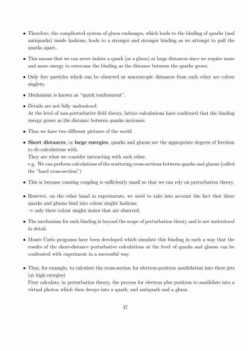
virtual photon which then decays into a quark, and antiquark and a gluon.
37
• The two Feynman diagrams for this process are:
e+
e−
q
q
γ∗ g e+
e−
q
q
γ∗
g
• However, before we can compare with experimental data we need to perform a convolution of this
calculated cross-section with a Monte Carlo.
This simulates the way in which the final state partons (quarks and gluons) bind with other quarks
and gluons to produce observed hadrons.
• It is only after such a convolution has been performed that one can get a reliable comparison of
the calculated cross-section with data.
• Likewise, if we want to calculate cross-sections for initial state hadrons we need to account for the
probability of finding a particular quark or gluon inside an initial hadron with a given fraction of
the initial hadron’s momentum (these are called “parton distribution functions”).
More later on the structure of hadrons.
4.5 θ− Parameter and Strong CP problem.
• There is one more gauge invariant term that can be added to the Lagrangian density for QCD.
This term is
Lθ = θαs8πǫµνρσF a
µνFaρσ = θ
αs8πF aµνF
aµν ,
where ǫµνρσ is the totally antisymmetric tensor (in four dimensions) and F is the dual field strength.
• Such a term arises when one considers “instantons” (which are beyond the scope of these lectures.)
• This term violates CP . In QED we would have
ǫµνρσFµνFρσ = E ·B,
and for QCD we have a similar expression except that Ea and Ba carry a colour index - they are
known as the chromoelectric and chromomagnetic fields.
38
• Under charge conjugation both the electric and magnetic filed change sign, but under parity the
electric field, which is a proper vector, changes sign, whereas the magnetic field, which is a polar
vector, does not change sign.
• Thus we see that the term E ·B is odd under CP .
• For this reason, the parameter θ in front of this term must be exceedingly small in order not to
give rise to strong interaction contributions to CP violating quantities such as the electric dipole
moment of the neutron.
• The current experimental limits on this dipole moment tell us that θ < 10−9 and it is probably
zero.
• Nevertheless, strictly speaking θ is a free parameter of QCD, and is often considered to be the
nineteenth free parameter of the Standard Model.
• Of course we simply could set θ = 0 (or a very small number), however term is regenerated
through loops
• Even if we could set it to zero we want to know why.
• The fact that we do not know why this term is absent (or so small) is the strong CP problem.
• Several possible solutions to the strong CP problem that offer explanations as to why this term
is absent (or small).
• One possible solution: add additional symmetry, leading to the postulation of a new, hypothetical,
weakly interacting particle, called the (Peccei-Quinn) axion.
• Unfortunately none of these solutions have been confirmed yet and the problem is still unresolved.
• Another question: why no problem in QED?
• This term can be written (in QED and QCD) as a total divergence, so it seems that it can be
eliminated from the Lagrangian altogether.
• However, in QCD (but not in QED) there are non-perturbative effects from the non-trivial topo-
logical structure of the vacuum (somewhat related to so called instantons you probably have heard
about) which prevent us from neglecting the θ-term
39

4.6 Summary
• Quarks transform as a triplet representation of colour SU(3) (each quark can have one of three
colours.)
• The requirement that the observed hadrons must be singlets of colour SU(3) solves the spin-
statistics problem for baryons. The wavefunction for a colour singlet state of three quarks has an
antisymmetric colour component.
• QCD is the SU(3) gauge theory in which the symmetry under colour SU(3) is taken to be local.
• The eight gauge bosons of QCD are the gluons which are the carriers that mediate the strong
interactions. They are massless.
• The coupling of quarks to gluons (and gluons to each other) decreases as the energy scale increases.
Therefore, at high energies one can perform reliable perturbative calculations for strong interacting
processes.
• As the distance between quarks increases the binding increases, such that it is impossible to isolate
individual quarks or gluons.
→ The only observable particles are colour singlet hadrons.
• Perturbative calculations performed at the quark and gluon level must be modified by account-
ing for the recombination of final state quarks and gluons into observed hadrons as well as the
probability of finding these quarks and gluons inside the initial state hadrons.
• QCD admits a gauge invariant strong CP violating term with a coefficient θ. This parameter
is known to be very small from limits on CP violating phenomena such as the electric dipole
moment of the neutron.
40
5 Spontaneous Symmetry Breaking
• We have seen that in an unbroken gauge theory the gauge bosons must be massless.
• The only observed massless spin-1 particles are photons. In the case of QCD, the gluons are also
massless, but they cannot be observed because of confinement.
• To extend the ideas of describing interactions by a gauge theory to the weak interactions, the
symmetry must somehow be broken since the carriers of weak interactions (W - and Z-bosons) are
massive (weak interactions are very short range).
• We could simply break the symmetry by hand by adding a mass term for the gauge bosons, which
we know violates the gauge symmetry.
• However, this would destroy renormalizability of our theory.
• Renormalizable theories are preferred because they are more predictive.
5.1 Massive gauge bosons and Renormalisability
• Show in a little more detail how explicit breaking mean non-renormalisability
• Higher order (loop) corrections generate ultraviolet divergences.
• In a renormalisable theory, these divergences can be absorbed into the parameters of the theory
and in this way can be ‘hidden’.
• As we go to higher orders we need to absorb more and more terms into these parameters, but
there are only as many divergent quantities as there are parameters.
• E.g. in the QED Lagrangian we have a fermion field, the gauge boson field and interactions whose
strength is controlled by e and m
• All divergences of diagrams can be absorbed into these quantities
• Once measured all other predictions can be written in terms of these parameters
• There are conditions on allowed terms in a renormalisable theory
• Furthermore all the propagators have to decrease like 1/p2 as the momentum p→ ∞.
41
• If conditions are not fulfilled then the theory generates more and more divergent terms as one
calculates to higher orders and it is not possible to absorb these divergences into the parameters
of the theory.
• Such theories are said to be “non-renormalisable”.
• So how does adding an explicit mass term M2AµAµ ruin renormalisabililty?
• This term modifies the propagator,
1
2Aµ(−gµν(p2 −M2) + pµpν
)Aν
inverting this we havei
p2 −M2
(gµν +
pµpν
M2
)
note that this propagator has a much worse UV behaviour, it goes to a constant as p → ∞.
compared to
−i(gµν − ξ
pµpν
p2
)1
p2
• With the explicit mass term the theory has more UV divergences
• It is the gauge symmetry that ensures renormalisabililty
• There is a far more elegant way of doing this which is called “spontaneous symmetry breaking”.
• In this scenario, the Lagrangian maintains its symmetry under a set of local gauge transformations.
• On the other hand, the lowest energy state, which we interpret as the vacuum state, is not a
singlet of the gauge symmetry.
• There is an infinite number of states each with the same ground-state energy and Nature chooses
one of these states as the ‘true’ vacuum.
5.2 Spontaneous Symmetry Breaking
• Spontaneous symmetry breaking is a phenomenon that is not restricted to gauge symmetries.
• In order to illustrate the idea of spontaneous symmetry breaking:
Consider a pen that is completely symmetric with respect to rotations around its axis.
42
• If we balance this pen on its tip on a table, and start to press on it with a force precisely along
the axis we have a perfectly symmetric situation.
• This corresponds to a Lagrangian which is symmetric (under rotations around the axis of the pen
in this case).
• However, if we increase the force, at some point the pen will bend (and eventually break).
• The question then is in which direction will it bend. Of course we do not know, since all directions
are equal.
• But the pen will pick one and by doing so it will break the rotational symmetry. This is sponta-
neous symmetry breaking.
• Better example can be given by looking at a point mass in a potential
V (r) = µ2r.r + λ(r.r)2
• Potential is symmetric under rotations and we assume λ > 0 (otherwise there would be no stable
ground state).
• For µ2 > 0 potential has a minimum at r = 0, thus the point mass will simply fall to this point.
• The situation is more interesting if µ2 < 0.
• For two dimensions the potential is a mexican hat potential.
• If the point mass sits at r = 0 the system is not in the ground state and is not stable but the
situation is completely symmetric.
• In order to reach the ground state, the symmetry has to be broken, i.e. if the point mass wants
to roll down, it has to decide in which direction.
• Any direction is equally good, but one has to be picked.
• This is exactly what spontaneous symmetry breaking means.
• The Lagrangian (here the potential) is symmetric (here under rotations around the z-axis), but
the ground state (here the position of the point mass once it rolled down) is not.
• Mathematically: Ground state is |0〉.
43
• A spontaneously broken gauge theory is a theory whose Lagrangian is invariant under gauge
transformations but ground state is not invariant under gauge transformations.
e−iωaT
a|0〉 6= 0
which means
T a|0〉 6= 0 for some a
• Thus the theory is spontaneously broken if at least one generator does not annihilate the vacuum
5.3 Spontaneous Symmetry Breaking
• We start by considering a complex scalar field theory with a mass term and a quartic self-
interaction.
• The Lagrangian density for such a theory may be written
L = ∂µΦ∗ ∂µΦ− V (Φ), (5.1)
where the “potential” V (Φ), is given by
V (Φ) = µ2Φ∗Φ+ λ |Φ∗Φ|2 . (5.2)
• This Lagrangian is invariant under global U(1) transformations
Φ → eiωΦ.
• Provided µ2 is positive this potential has a minimum at Φ = 0.
• We call the Φ = 0 state the vacuum and expand Φ in terms of creation and annihilation operators
that populate the higher energy states.
• In terms of a Quantum Field Theory, where Φ is an operator, the precise statement is that the
operator, Φ, has zero “vacuum expectation value”.
• Suppose now that we reverse the sign of µ2, so that the potential becomes
V (Φ) = −µ2Φ∗Φ + λ |Φ∗Φ|2 . (5.3)
44
φ
φ|φ |0
V
Re
Im
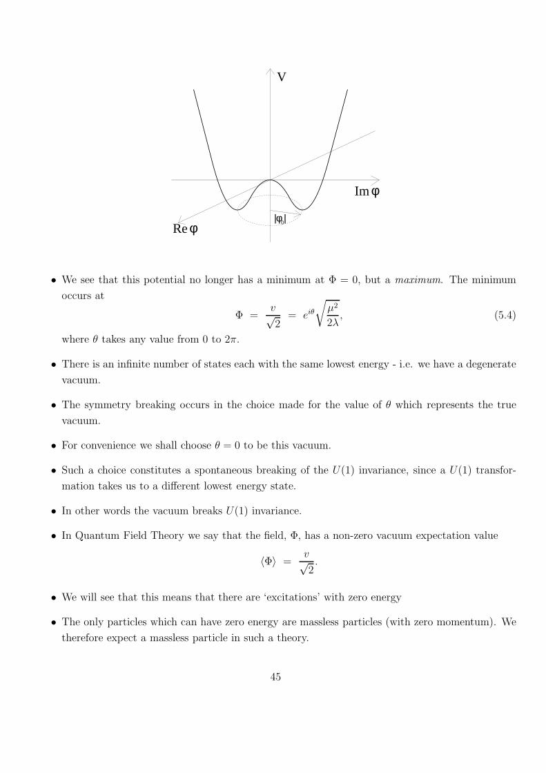
• We see that this potential no longer has a minimum at Φ = 0, but a maximum. The minimum
occurs at
Φ =v√2
= eiθ√µ2
2λ, (5.4)
where θ takes any value from 0 to 2π.
• There is an infinite number of states each with the same lowest energy - i.e. we have a degenerate
vacuum.
• The symmetry breaking occurs in the choice made for the value of θ which represents the true
vacuum.
• For convenience we shall choose θ = 0 to be this vacuum.
• Such a choice constitutes a spontaneous breaking of the U(1) invariance, since a U(1) transfor-
mation takes us to a different lowest energy state.
• In other words the vacuum breaks U(1) invariance.
• In Quantum Field Theory we say that the field, Φ, has a non-zero vacuum expectation value
〈Φ〉 =v√2.
• We will see that this means that there are ‘excitations’ with zero energy
• The only particles which can have zero energy are massless particles (with zero momentum). We
therefore expect a massless particle in such a theory.
45
• To see this, we expand Φ around its vacuum expectation value as
Φ =1√2
(µ√λ+H + iφ
). (5.5)
• The fields H and φ have zero vacuum expectation value and it is these fields that are expanded
in terms of creation and annihilation operators of the particles that populate the excited states.
• Now insert (5.5) into (5.3) we find
V = µ2H2 + µ√λ(H3 + φ2H
)+λ
4
(H4 + φ4 + 2H2 φ2
)+µ4
4λ. (5.6)
• Note that in (5.6) there is a mass term for the field H , but no mass term for the field φ. Thus φ
is a field for a massless particle called a “Goldstone boson”.
• The field H will be “held” in a restoring potential, which corresponds precisely to a genuine mass
term.
• On the other hand, in the φ direction at this point, the field will be moving along the “valley” of
the potential which means that it’s a massless field when quantized.
46
5.4 Goldstone Bosons
• Goldstones theorem extends this to spontaneous breaking of a general symmetry.
• Suppose we have a theory which is invariant under a symmetry group G with N generators
• Assume some operator (i.e. a function of the quantum fields - which might just be a component
of one of these fields) has a non-zero vacuum expectation value, which breaks the symmetry down
to a subgroup H of G, with n generators
• The vacuum state is still invariant under transformations generated by the n generators of H, but
not the remaining N − n generators of the original symmetry group G.
• Thus we have
T a|0〉 = 0, a = 1...n , T a|0〉 6= 0, a = n+ 1...N
• Goldstone’s theorem states that there will be N − n massless particles (one for each broken
generator of the group).
• The case considered in this section is special in, there is only one generator of the symmetry group
(i.e. N = 1) which is broken by the vacuum.
• Thus, there is no generator that leaves the vacuum invariant (i.e. n = 0) and we get N − n = 1
Goldstone boson.
• The quantum numbers of the Goldstone particle are the same as the corresponding generator
For example: Global transformations are usually internal transformations in field space not touch-
ing Lorentz indices
→ Generators are Lorentz scalars - Goldstones are scalars
• Not true in SUSY; generators of SUSY transformations are fermionic - massless particles are
fermions - Goldstinos.
5.5 The Higgs Mechanism
• Goldstone’s theorem has a loophole, which arises when one considers a gauge theory, i.e. when
one allows the original symmetry transformations to be local.
• In a spontaneously broken gauge theory, the choice of which vacuum is the true vacuum is equiv-
alent to choosing a gauge, which is necessary in order to be able to quantise the theory.
47
• What this means is that the Goldstone bosons, which can, in principle, transform the vacuum
into one of the states degenerate with the vacuum, now affect transitions into states which are
not consistent with the original gauge choice.
• This means that the Goldstone bosons are “unphysical” and are often called “Goldstone ghosts”.
• On the other hand the quantum degrees of freedom associated with the Goldstone bosons are
certainly there before a choice of gauge is made. What happens to them?
• To see how this works we return to the U(1) global theory, but now we promote the symmetry to
a local symmetry (hence to a gauge theory)
• We must introduce a gauge boson, Aµ. The partial derivative of the field Φ is replaced by a
covariant derivative
∂µΦ → DµΦ = (∂µ + i g Aµ) Φ.
Including the kinetic term −14FµνF
µν for the gauge bosons, the Lagrangian density becomes
L = −1
4FµνF
µν + (DµΦ)∗DµΦ− V (Φ) (5.7)
• Now note what happens if we insert the expansion
Φ =1√2(v +H + iφ)
into the term (DµΦ)∗DµΦ. This generates the following terms
(DµΦ) (DµΦ)∗ =
[(∂µ + igAµ)
(1√2(v +H + iφ)
)][(∂µ − igAµ)
(1√2(v +H − iφ)
)]
=
[1√2∂µH +
i√2∂µφ+
ig√2vAµ +
ig√2AµH − g√
2Aµφ
]
×[
1√2∂µH − i√
2∂µφ− ig√
2vAµ − ig√
2AµH − g√
2Aµφ
]
=1
2∂µH ∂µH +
1
2∂µφ ∂
µφ+1
2g2v2AµA
µ
+1
2g2AµA
µ(H2 + φ2
)− g Aµ (φ ∂µH − H ∂µφ) + g v Aµ∂µφ+ g2 v AµAµH,
(where v = µ/√λ). The gauge boson has acquired a mass term,
MA = g v,
48
• There is a coupling of the gauge field to the H-field,
g2vAµAµH = gMAAµA
µH
• There is also the bilinear term
gvAµ∂µφ
which after integrating by parts (for the action S) may be written as
−MAφ∂µAµ
• This mixes the Goldstone boson, φ, with the longitudinal component of the gauge boson, with
strength MA
• Explicitly,
MAφ∂µAµ =MAφ∂
µ(ALµ + ATµ ) =MAφ∂µALµ
as ∂µATµ = 0.
• Later on, we will use the gauge freedom to get rid of this mixing term.
• A massless vector boson has only two degrees of freedom (the two directions of polarisation of a
photon)
• A massive vector (spin-one) particle has three possible values for the helicity of the particle, 2
transverse and 1 longitudinal
• In a spontaneously broken gauge theory, the Goldstone boson associated with each broken gener-
ator provides the third degree of freedom to the gauge bosons.
→ This means that the gauge bosons become massive.
• The Goldstone boson is said to be “eaten” by the gauge boson.
• This is related to the mixing term between ALµ and φ
• Thus, in our abelian model, the two degrees of freedom of the complex field Φ turn out to be the
Higgs field and the longitudinal component of the (now massive) gauge boson.
• There is no physical, massless particle associated with the degree of freedom φ present in Φ.
49
5.6 Gauge Fixing
• Going back to the bilinear term
MAφ∂µALµ
we can think of the longitudinal component of the gauge boson oscillating between the Goldstone
boson due to this mixing term
→ the physical particle is described by a superposition of these fields.
We consider two special cases:
The unitary gauge:
• The physical field for the longitudinal component of the gauge boson is not simply ALµ , but the
superposition
Aphµ = Aµ +1
MA∂µφ. (5.8)
(Note that this only affects the longitudinal component).
• Now all the terms quadratic in Aµ, φ (including the bilinear mixing term) may be written (in
momentum space) as
Aphµ (−p)(−gµν p2 + pµpν + gµνM2
A
)Aphν (p). (5.9)
• Writing out the Lagrangian we notice that the Goldstone boson field, φ, has disappeared. The
terms involving φ in the original expression have been absorbed (or “eaten”) by the redefinition
(5.8) of the gauge field.
• The gauge boson propagator is the inverse of the coefficient of (dropping the superscript ph)
Aµ(−p)Aν(p) in (5.9) , which is
−i(gµν −
pµpνM2
A
)1
(p2 −M2A), (5.10)
which is the usual expression for the propagator of a massive spin-one particle.
• The only other remaining particle is the scalar, H, with mass mH =√2µ which is called the
“Higgs” particle
• This is a physical particle, which interacts with the gauge boson and also has cubic and quartic
self-interactions.
50
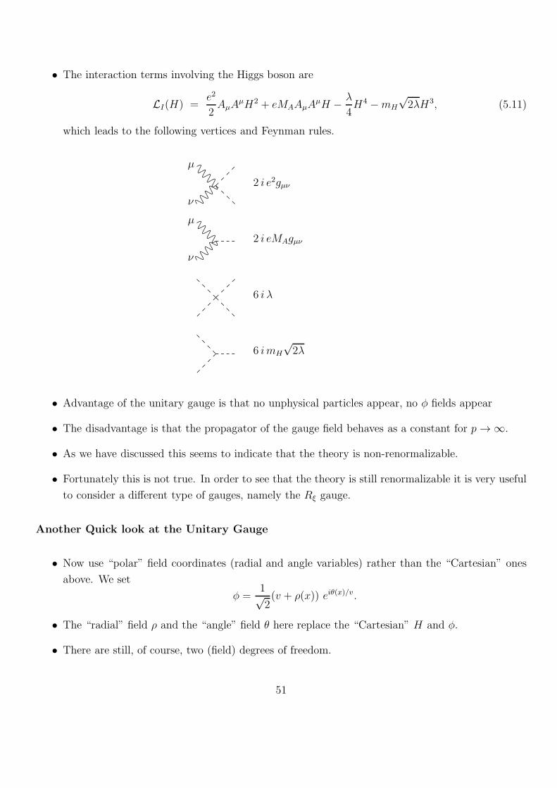
• The interaction terms involving the Higgs boson are
LI(H) =e2
2AµA
µH2 + eMAAµAµH − λ
4H4 −mH
√2λH3, (5.11)
which leads to the following vertices and Feynman rules.
µ
ν
µ
ν
2 i e2gµν
2 i eMAgµν
6 i λ
6 imH
√2λ
• Advantage of the unitary gauge is that no unphysical particles appear, no φ fields appear
• The disadvantage is that the propagator of the gauge field behaves as a constant for p→ ∞.
• As we have discussed this seems to indicate that the theory is non-renormalizable.
• Fortunately this is not true. In order to see that the theory is still renormalizable it is very useful
to consider a different type of gauges, namely the Rξ gauge.
Another Quick look at the Unitary Gauge
• Now use “polar” field coordinates (radial and angle variables) rather than the “Cartesian” ones
above. We set
φ =1√2(v + ρ(x)) eiθ(x)/v.
• The “radial” field ρ and the “angle” field θ here replace the “Cartesian” H and φ.
• There are still, of course, two (field) degrees of freedom.
51
• Stick this into L and find
L = (1
2∂µρ ∂
µρ − 1
2µ2ρ2) + (
1
2∂µθ ∂
µθ) +ρ
v∂µθ ∂
µθ + other interaction terms.
• The “θ” mode is the one for motion around the equilibrium circle, and it is massless.
• The “ρ” mode (radial) is restored, and has mass µ.
• Now make the global U(1) symmetry of this model into a local symmetry by introducing a U(1)
gauge field
• This is the Abelian Higgs model.
• We have to change all derivatives to covariant derivatives and add in the Maxwell term for the
Aµ field. This produces
L = [(∂µ + igAµ)φ]† [(∂µ + igAµ)φ] − 1
4FµνF
µν +1
2µ2 | φ |2 − 1
2λ2 | φ |4 .
• As in the Goldstone model, expand about a point on the equilibrium circle as before
• This time we shall choose to use the “polar” field variables, and write
φ =1√2(v + ρ(x)) eiθ(x)/v
where v = µ/λ.
• The theory is invariant under the combined transformations
φ→ φ′ = e−iχ(x) φ
and
Aµ → A′µ = Aµ +
1
g∂µχ,
where χ is arbitrary.
• The fields ρ and θ transform by
ρ→ ρ
and
θ → θ − vχ.
• So, we can choose the field χ to be θ/v and so θ vanishes!
52
• That is, we can choose a gauge in which φ is real.
• Remember that the gauge transformation affects the gauge field Aµ and the complex scalar field
φ simultaneously.
• After the gauge transformation in which θ is reduced to zero, Aµ is changed to
A′µ = Aµ +
1
gv∂µθ
and φ is
φ′ =1√2(v + ρ).
• L in terms of these primed fields is then
L(φ′, A′µ) = (
1
2∂µρ ∂
µρ − 1
2µ2ρ2) − 1
4F ′µνF
′µν +1
2g2v2A′
µA′µ + interactions.
• ρ has a genuine mass µ.
• But where is the massless mode θ?
• It has been “eaten” by the Aµ field!
• It is present in A′µ via
A′µ = Aµ +
1
gv∂µθ.
• A′µ is a massive spin-1 particle, of mass gv!
• This is the Higgs mechanism, whereby the massless gauge field Aµ has become a massive spin-1
field A′µ by “eating” the scalar field θ.
• θ = 0 is physically appealing and is called the “unitary gauge”.
Rξ Feynman gauge:
• We select the Feynman gauge by adding to the Lagrangian density the term
LR ≡ − 1
2(1− ξ)(∂ · A− (1− ξ)MAφ)
2
= − 1
2(1− ξ)∂µA
µ∂νAν +MAφ∂µA
µ − 1− ξ
2M2
Aφ2
53
• The cross-term MAφ ∂µAµ cancels the bilinear mixing term.
• Again, the special value ξ = 0 corresponds to the Feynman gauge.
• The quadratic terms in the gauge boson are
1
2Aµ(−p)
(−gµν(p2 −M2
A) + pµpν −pµpν1− ξ
)Aν(p)
leading to the propagator
−i(p2 −M2
A)
(gµν − ξ
pµpνp2 − (1− ξ)M2
A
)
• in the Feynman gauge the gauge boson propagator simplifies to
−i gµν(p2 −M2
A), (5.12)
which is easy to handle.
• There is, however, a price to pay. The Goldstone boson is still present.
• It has acquired a mass, MA, from the gauge fixing term, and it has interactions with the gauge
boson, with the Higgs scalar and with itself.
• Furthermore, for the purposes of higher order corrections in non-abelian theories we again need
to introduce Faddeev-Popov ghosts which in this case interact not only with the gauge boson, but
also with the Higgs scalar and Goldstone boson.
5.7 Bit more on Renormalisability
• Recalling the form of the gauge boson propagator fir the Unitary gauge
−i(gµν −
pµpνM2
A
)1
(p2 −M2A)
(5.13)
we see that it does not decrease as p→ ∞
• This would normally lead to a violation of renormalisability, thereby rendering the Quantum Field
Theory useless
• However, there is no contradiction between the apparent non-renormalizability of the theory in
the unitary gauge and the manifest renormalizability in the Rξ gauge.
54
• Physical quantities are gauge invariant, any physical quantity can be calculated in a gauge where
renormalizability is manifest.
• The price we pay for this is that there are more particles and many more interactions, leading to
a plethora of Feynman diagrams.
• Only work in such gauges if we want to compute higher order corrections.
• For the rest of these lectures we shall confine ourselves to tree-level calculations and work solely
in the unitary gauge.
• Nevertheless, one cannot over-stress the fact that it is only when the gauge bosons acquire masses
through the Higgs mechanism that we have a renormalizable theory.
55
5.8 Spontaneous Symmetry Breaking in a Non-Abelian Gauge Theory
• Extend to non-Abelian gauge theories.
• Take an SU(2) gauge theory and consider a complex doublet of scalar fields. Φi, i = 1, 2.
• The Lagrangian density is
L = −1
4F aµνF
aµν + |DµΦ|2 − V (Φ), (5.14)
where
DµΦ = ∂µΦ+ i g W aµ T
aΦ,
(we have changed notation for the gauge bosons from Aaµ to W aµ ), and
V (Φ) = −µ2Φ†iΦ
i + λ(Φ†iΦ
i)2. (5.15)
• This potential has a minimum at Φ†iΦi =
12µ2/λ.
• We choose the vacuum expectation value to be in the T 3 = −12direction and to be real, i.e.
〈Φ〉 =1√2
(0
v
),
(v = µ/√λ).
• This vacuum expectation value is not invariant under any SU(2) transformation.
• This means that there is no unbroken subgroup
• Counting goes as follows: We start with 2 component complex scalar = 4 dof
three generators are broken = three Goldstone bosons with all three of the gauge bosons acquiring
a mass
one dof left which is the massive Higgs scalar.
• We expand Φi about its vacuum expectation value (“vev”)
Φ =1√2
(φ1 − i φ2
v + H + i φ0
).
• The φa, a = 0 · · ·2 are the three Goldstone bosons and H is the physical Higgs scalar.
56
• All of these fields have zero vev.
• If we insert this expansion into the potential (5.15) then we find that we only get a mass term for
the Higgs field, with value mH =√2µ.
• For simplicity, move directly into the unitary gauge by setting all the three φa to zero.
• In this gauge DµΦ may be written
DµΦ =1√2
(∂µ
(0
H
)+ i
g
2
(W 3µ W 1
µ − iW 2µ
W 1µ + iW 2
µ −W 3µ
)(0
v +H
))
1√2
(∂µ
(0
H
)+ i
g
2
(W 0µ
√2W+
µ√2W−
µ −W 0µ
)(0
v +H
)),
where we have introduced the notation W±µ = (W 1
µ ∓ iW 2µ)/
√2, W 0
µ = W 3µ and used the explicit
form for the generators of SU(2) in the 2× 2 representation given by the Pauli matrices.
• The term |DµΦ|2 then becomes
|DµΦ|2 =1
2∂µH ∂µH +
1
4g2v2
(W+µ W
−µ +1
2W 0µW
0µ
)
+1
4g2H2
(W+µ W
−µ +1
2W 0µW
0µ
)+
1
2g2vH
(W+µ W
−µ +1
2W 0µW
0µ
). (5.16)
• We see from the terms quadratic in Wµ that all three of the gauge bosons have acquired a mass
MW =gv
2
57
6 Spontaneous Breaking of SU(2)L × U(1)Y → U(1)EM
• Consider the particle content just consisting of one Higgs doublet, Φ and the gauge fields associated
with the SU(2)L × U(1)Y
• Higgs has quantum number (2, 12) and has the form
Φ =
(h+
h0
)
• The Lagrangian for this is then
L = −1
4F aµνF
aµν − 1
4GµνG
µν + |DµΦ|2 − V (Φ) (4 d.o.f)
where
F aµν = ∂µW
aν − ∂νW
aµ − g fabcW b
µWcν
Gµν = ∂µBν − ∂νBµ
DµΦ = ∂µ +ig′
2Bµ +
ig
2τ iW i
µ
V (Φ) = −µ2Φ†iΦ
i + λ(Φ†iΦ
i)2
where τ is are the Pauli matrices.
• Expanding the Higgs field around its VEV In the Unitary gauge the covariant derivative takes
the form
DµΦ =1√2
(∂µ + i
g
2
(W 0µ
√2W+
µ√2W−
µ −W 0µ
)+ i
g′
2Bµ
)(0
v + H
)(6.1)
=1√2
(∂µ + i g
2W 0µ + i g
′
2Bµ i g
2
√2W+
µ
i g2
√2W−
µ ∂µ − i g2W 0µ + i g
′
2Bµ
)(0
v + H
)
=1√2
(i g2
√2W+
µ (v +H)
(∂µ − i g2W 0µ + i g
′
2Bµ)(v +H)
)
where we have taken W±µ =
W 1µ∓iW 2
µ√2
and W 0µ = W 3
µ . We then get
|DµΦ|2 =1
2(∂µH)2 +
g2v2
4W+µW−
µ +v2
8
(gW 0
µ − g′Bµ
)2+
g2
4W+µW−
µ (2vH +H2) +1
8
(gW 0
µ − g′Bµ
)2(2vH +H2) . (6.2)
58
• We get a mass terms for the charged gauge boson and a linear combination(gW 0
µ − g′Bµ
).
• We need to diagonalise the W 0µ −B0
µ system and we can do that by introducing
Zµ = cos θwW0µ − sin θwBµ
Aµ = sin θwW0µ + cos θwBµ
i.e.
Bµ = cos θwAµ − sin θwZµ
W 0µ = sin θwAµ + cos θwZµ
where
tan θw =g′
g
• Now our non-interaction part of the Lagrangian is given by
Lnon−int =1
2
((∂.H)2 − µ2H2
)
− 1
4
(∂µW
1ν − ∂νW
1µ
) (∂µW ν1 − ∂νW µ1
)+
1
8g2v2W 2
1
− 1
4
(∂µW
2ν − ∂νW
2µ
) (∂µW ν2 − ∂νW µ2
)+
1
8g2v2W 2
2
− 1
4(∂µZν − ∂νZµ) (∂
µZν − ∂νZµ) +1
8(g2 + g′
2
)v2Z2
− 1
4(∂µAν − ∂νAµ) (∂
µAν − ∂νAµ)
• The physical interpretation of this is the following: 3 massive vector particles
M1 =M2 =gv
2=MW±
andv
2(g2 + g′
2
)1/2 =vg
2
1
cos θw=MW±
cos θw=MZ
• We also have one massless vector and a massive Higgs
• The masslessness of Aµ follows from the choice of breaking condition, i.e. the form of the vev.
59
• There is a combination of the original generators that still annihilates the the vacuum, i.e. there is
a linear combinations of generators that is still invariant - one gauge symmetry not spontaneously
broken(Y +
T32
)(0
v/√2
)=
[(1/2 0
0 1/2
)+
(1/2 0
0 −1/2
)](0
v/√2
)
=
(1 0
0 0
)(0
v/√2
)=
(0 0
0 0
)
• We can rewrite this linear combination in terms of the isospin τ3 = 2tisospin3 so that the linear
combination is
Y + tisospin3
• Going back to the covariant derivative for the doublet Φ we have
DµΦ = ∂µΦ +ig′
2BµΦ +
ig
2τ iW i
µΦ
= ∂µΦ +ig′
2(cos θwAµ − sin θwZµ)Φ +
ig
2(τ 3 sin θwAµ + cos θwZµ)Φ +W 1, W 2 bits
= ∂µΦ +ig
2tan θw (cos θwAµ − sin θwZµ) Φ +
ig
2(τ 3 sin θwAµ + cos θwZµ)Φ
= ∂µΦ +ig
2sin θw(1 + τ 3)AµΦ+
ig
cos θw
(τ 3
2− sin2 θw
(1 + τ 3)
2
)ZµΦ
⇒ Dµ = ∂µ + ig sin θw
(1
2+ tisospin3
)Aµ +
ig
cos θw
(τ 3
2− sin2 θw
(1 + τ 3)
2
)Zµ
We then of course identify
g sin θw
(1
2+ tisospin3
)= eQ(Φ)
with
g sin θw = e
and
Q(Φ) =1
2+ tisospin3
• We can see this makes sense as
g sin θw
(1
2+ tisospin3
)Φ = g sin θw
(1
2+ tisospin3
)(h+
h0
)
= g sin θw
(1 0
0 0
)(h+
h0
)= e
(Q 0
0 0
)(h+
h0
)(6.3)
if we are to identify Aµ as the photon
60
6.1 More on renormalisability
Electroweak theory is renormalisable
• Hopefully the LHC will determine whether the simplest Higgs model is correct
• Higgs is motivated by theory - no experimental evidence - or for any fundamental scalar.
• Allows us to introduce weak boson masses without spoiling renormalisability of electroweak theory
• We have seen a rough argument with propagators but we can also see the effects in diagrams.
• Structure of lowest-order amplitudes for weak processes hints that we may have trouble without
the Higgs.
• Consider the cross section
σ(νee→ νee) =G2s
π
• Becomes infinite as s→ ∞.
• This cannot be true for large s as this violates unitarity.
• Can solve this by introducing a W mass and now for large s we have a diagram
σ
e− νe
νe
W
e−
=G2M2
W
π
• However the introduction of the W boson causes problems due to the diagram
σ
W− W−
νe
e−
νe
=G2s
3π
which diverges at large s.
61
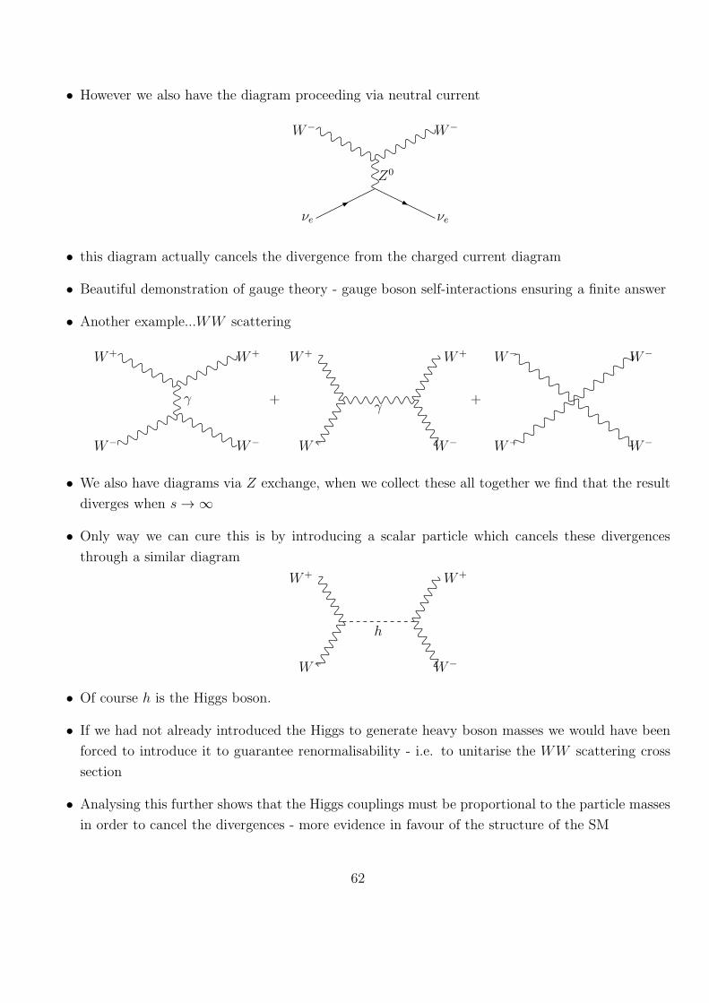
• However we also have the diagram proceeding via neutral current
W− W−
νe
Z0
νe
• this diagram actually cancels the divergence from the charged current diagram
• Beautiful demonstration of gauge theory - gauge boson self-interactions ensuring a finite answer
• Another example...WW scattering
W+ W+
W−
γ
W−
+
W+ W+
W−
γ
W−
+
W− W−
W− W−
• We also have diagrams via Z exchange, when we collect these all together we find that the result
diverges when s→ ∞
• Only way we can cure this is by introducing a scalar particle which cancels these divergences
through a similar diagram
W+ W+
W−
h
W−
• Of course h is the Higgs boson.
• If we had not already introduced the Higgs to generate heavy boson masses we would have been
forced to introduce it to guarantee renormalisability - i.e. to unitarise the WW scattering cross
section
• Analysing this further shows that the Higgs couplings must be proportional to the particle masses
in order to cancel the divergences - more evidence in favour of the structure of the SM
62
6.2 Summary
• For a field theory in which the potential is not a minimum when all the fields take the value zero,
at least one of the fields acquires a non-zero vacuum expectation value (vev).
• The symmetry is said to be spontaneously broken because one of many degenerate ground states
is chosen to be the true vacuum.
• There may, in general, be a subset of transformations (i.e. a subgroup H of the original symmetry
group G) under which the vev is invariant.
• The vacuum is then invariant under this subgroup H and we say that the original symmetry
described by the group G has been spontaneously broken to the subgroup H.
• When a field, in a theory that is invariant under a set of transformations, acquires a vacuum
expectation value there is a massless Goldstone boson for each generator of the symmetry, which
is broken by that expectation value.
• These Goldstone bosons are the ‘excitations’ which effect transitions to the other states, which
are degenerate with the vacuum.
• In the case of a gauge theory these Goldstone bosons provide the longitudinal component of the
gauge bosons, which therefore acquire a mass.
• The mass is proportional to the magnitude of the vacuum expectation value and the gauge coupling
constant.
• The Goldstone bosons themselves are unphysical.
• One can work in the unitary gauge where the Goldstone boson fields are set to zero.
• When gauge bosons acquire masses by this (Higgs) mechanism, renormalisability is maintained.
• This can be seen explicitly if one works in a gauge other than the unitary gauge, in which the gauge
boson propagator decreases as 1/p2 as p→ ∞, which is a necessary condition for renormalisability.
• If one does work in such a gauge, however, one needs to work with Goldstone boson fields, even
though the Goldstone bosons are unphysical.
• The number of interactions and the number of Feynman graphs required for the calculation of
some process is greatly increased.
63
7 The Electroweak Model of Leptons
• Only one or two modifications are needed to the model described at the end of the last lecture to
obtain the Glashow-Weinberg-Salam (GWS) model of electroweak interactions.
• This was the first model that successfully unified different forces of Nature.
• In this lecture we shall consider only leptons as matter fields, deferring the introduction of hadrons
to the next lecture.
7.1 Left- and right- handed fermions
• The weak interactions are known to violate parity
→ they are not symmetric under interchange of left-helicity and right-helicity fermions.
First Recall a few things about writing Lagrangians in terms of Weyl and Dirac spinors.
• A Dirac field, ψ, representing a fermion, can be expressed as the sum of a left-handed part, ψL,
and a right-handed part, ψR,
ψ = ψL + ψR, (7.1)
where
ψL = PL ψ
PL =(1− γ5)
2(7.2)
ψR = PR ψ
PR =(1 + γ5)
2(7.3)
PL and PR are projection operators in the sense that
PL PL = PL, PR PR = PR, and PL PR = 0. (7.4)
• They project out the left-handed (negative) and right-handed (positive) helicity states of the
fermion respectively.
64
• The kinetic term of the Dirac Lagrangian and the interaction term of a fermion with a vector field
can also be written as a sum of two terms each involving only one helicity.
ψ γµ∂µψ = ψL γµ∂µψL + ψR γ
µ∂µψR, (7.5)
ψ γµAµψ = ψL γµAµψL + ψR γ
µAµψR. (7.6)
• On the other hand, a mass term mixes the two helicities
mψψ = mψL ψR + mψR ψL.
• Thus, if the fermions are massless, we can treat the left-handed and right-handed helicities as
separate particles.
• We can understand this physically:
Massive fermion moving along the positive z-axis with spin positive component, so that the helicity
is positive in this frame
• Can always boost into a frame with the fermion moving along the negative z-axis, but the com-
ponent of spin is unchanged, helicity will be negative.
• For massless particle it travels with the speed of light no such boost is possible and in that case
the helicity is a good quantum number.
• Since charged weak interactions are observed to occur only between left-helicity fermions, we
consider a weak isospin, SU(2), under which the left-handed leptons transform as a doublet
LL =
(νL
eL
),
under this SU(2), but the right-handed electron eR is a singlet.
• i.e
eR → e′R = eR
where as
LL → L′L = e−ω
aTa
LL
• Under U(1)Y gauge transformations
eR → e′R = e−ωY (eR)eR
65
where as
LL → L′L = e−ωY (LL)LL
with
Y (eR) = −1 and Y (LL) = −1
2
• Since this separation of the electron into its left- and right-handed helicity only makes sense for a
massless electron we also need to assume that the electron is massless in the exact SU(2) limit
• Also that the mass for the electron arises as a result of spontaneous symmetry breaking in the
same way that the masses for the gauge bosons arise.
7.2 Fermion masses - Yukawa couplings
• Cannot have explicit mass terms for the electrons since a mass term mixes left-handed and right-
handed fermions
• Is not gauge invariant.
• Can have an interaction between the left-handed lepton doublet, the right-handed electron and
the scalar doublet Φ.
• Such an interaction is called a “Yukawa interaction” and is written
LY ukawa = −λe lLiΦieR + h.c. (7.7)
Note that this term has zero weak hypercharge. In the unitary gauge this is
− λe√2
(νL eL
)( 0
v + H
)eR + h.c..
The part proportional to the vev is simply
− λe v√2
(eL eR + eR eL) = − λe v√2
(ePR e+ ePL e) =λe v√2e e,
and we see that the electron has acquired a mass, which is proportional to the vev of the scalar
field.
• This immediately gives us a relation for the Yukawa coupling in terms of the electron mass, me,
and the W−mass, MW ,
λe = gme√2MW
.
66
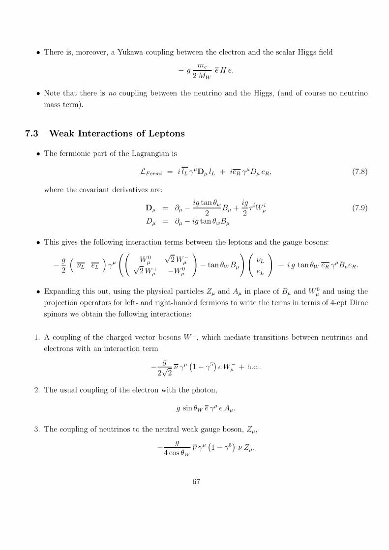
• There is, moreover, a Yukawa coupling between the electron and the scalar Higgs field
− gme
2MW
eH e.
• Note that there is no coupling between the neutrino and the Higgs, (and of course no neutrino
mass term).
7.3 Weak Interactions of Leptons
• The fermionic part of the Lagrangian is
LFermi = i lL γµDµ lL + ieR γ
µDµ eR, (7.8)
where the covariant derivatives are:
Dµ = ∂µ −ig tan θw
2Bµ +
ig
2τ iW i
µ (7.9)
Dµ = ∂µ − ig tan θwBµ
• This gives the following interaction terms between the leptons and the gauge bosons:
− g
2
(νL eL
)γµ
((W 0µ
√2W−
µ√2W+
µ −W 0µ
)− tan θWBµ
)(νL
eL
)− i g tan θW eR γ
µBµeR.
• Expanding this out, using the physical particles Zµ and Aµ in place of Bµ and W 0µ and using the
projection operators for left- and right-handed fermions to write the terms in terms of 4-cpt Dirac
spinors we obtain the following interactions:
1. A coupling of the charged vector bosons W±, which mediate transitions between neutrinos and
electrons with an interaction term
− g
2√2ν γµ
(1− γ5
)eW−
µ + h.c..
2. The usual coupling of the electron with the photon,
g sin θW e γµ eAµ.
3. The coupling of neutrinos to the neutral weak gauge boson, Zµ,
− g
4 cos θWν γµ
(1− γ5
)ν Zµ.
67
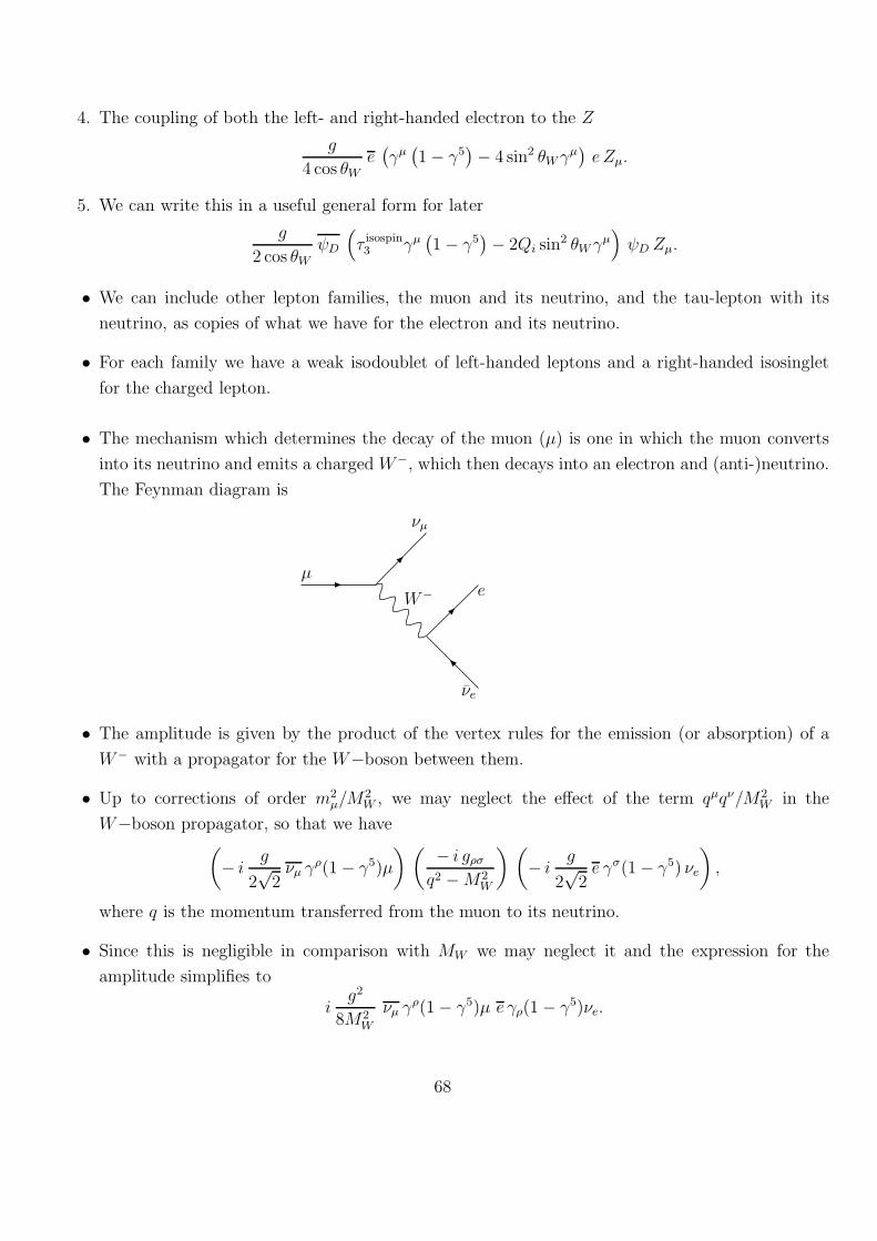
4. The coupling of both the left- and right-handed electron to the Z
g
4 cos θWe(γµ(1− γ5
)− 4 sin2 θWγ
µ)e Zµ.
5. We can write this in a useful general form for later
g
2 cos θWψD
(τ isospin3 γµ
(1− γ5
)− 2Qi sin
2 θWγµ)ψD Zµ.
• We can include other lepton families, the muon and its neutrino, and the tau-lepton with its
neutrino, as copies of what we have for the electron and its neutrino.
• For each family we have a weak isodoublet of left-handed leptons and a right-handed isosinglet
for the charged lepton.
• The mechanism which determines the decay of the muon (µ) is one in which the muon converts
into its neutrino and emits a charged W−, which then decays into an electron and (anti-)neutrino.
The Feynman diagram is
µ
νµ
νe
eW−
• The amplitude is given by the product of the vertex rules for the emission (or absorption) of a
W− with a propagator for the W−boson between them.
• Up to corrections of order m2µ/M
2W , we may neglect the effect of the term qµqν/M2
W in the
W−boson propagator, so that we have(− i
g
2√2νµ γ
ρ(1− γ5)µ
) ( − i gρσq2 −M2
W
) (− i
g
2√2e γσ(1− γ5) νe
),
where q is the momentum transferred from the muon to its neutrino.
• Since this is negligible in comparison with MW we may neglect it and the expression for the
amplitude simplifies to
ig2
8M2W
νµ γρ(1− γ5)µ e γρ(1− γ5)νe.
68
• Before the development of this model, weak interactions were described by the “four-fermi model”
with a weak interaction Hamiltonian given by
Hijkl =GF√2ψi γ
µ(1− γ5)ψj ψk γµ(1− γ5)ψl.
• This is an effective low-energy theory which may be used when the energy scales q ≪MW .
• The Fermi coupling constant, GF is related to the electric charge, e, the W−mass and the weak
mixing angle by
GF =e2
4√2M2
W sin2 θW. (7.10)
• This gives us a value for GF ,
GF = 1.12× 10⁻⁵ GeV−2
which is very close to the value of 1.17× 10⁻⁵ GeV−2 measured from the lifetime of the muon.
• Weak interactions are ‘weak’, not because the coupling is particularly small (the SU(2) gauge
coupling is about twice as large as the electromagnetic coupling), but because the exchanged
boson is very massive, so that the Fermi coupling constant of the four-fermi theory is very small.
• The large mass of the W−boson is also responsible for the fact that the weak interactions are
short range (of order 10−18 m).
• In SM we also have neutral weak currents.
• For example, we can have elastic scattering of muon-type neutrinos against electrons via the
exchange of the Z−boson.
• The Feynman diagram for such a process is
νµ
νµ
ee
Z
69
7.4 Classifying the Free Parameters
The free parameters in the GWS model for one generation of leptons are
• The two gauge couplings for the SU(2) and U(1) gauge groups, g and g′.
• The two parameters, µ and λ in the scalar potential V (Φ)
• The Yukawa coupling constant, Ge.
• It is convenient to replace these five parameters by five parameters which are directly measurable
experimentally, namely e, sin θW , and three masses mH , MW , me.
• The relation between these “physical” parameters and the parameters that one writes down in
the initial Lagrangian are
tan θW =g′
g,
e = g sin θW ,
mH =√2µ,
MW =g µ
2√λ,
me = Geµ√λ.
• Note that when we add more generations of leptons we acquire one more parameter for each added
generation, namely the Yukawa coupling, which determines the mass of the charged lepton.
• In terms of these measured quantities, the Z−mass, MZ , and the Fermi-coupling, GF are predic-
tions (although historically GF was known for many years before the discovery of the W−boson
and its value was used to predict the W−mass).
7.5 Summary
• Weak interactions are mediated by the gauge bosons of weak isospin which acts only on the
left-handed helicity components of fermions.
• The neutrino and left-handed component of the electron form a doublet of this weak isospin
whereas the right-handed component of the electron is a singlet.
70
• There is also a weak hypercharge U(1) gauge symmetry. Both left- and right-handed leptons
transform under this U(1) with a hypercharge which is related to the electric charge of the electron
by the relation
Q = Y + tisospin3
• The scalar multiplet which is responsible for the spontaneous symmetry breaking also carries weak
hypercharge.
• As a result of this neutral gauge bosons mix in such a way that the superposition
cos θwW0µ − sin θwBµ
acquires a mass whereas its orthogonal superposition
sin θwW0µ + cos θwBµ
remains massless.
• The massive particle is the Z−boson and the massless particle is the photon.
• The magnitude of the electron charge, e, is then given by e = g sin θW .
• The weak interactions proceed via the exchange of massive charged or neutral gauge bosons.
• The old four-fermi weak Hamiltonian is an effective Hamiltonian which is valid for low energy
processes in which all momenta are small compared with the W−mass.
• The Fermi coupling is obtained in terms of e, MW and sin θW by the relation
GF =e2
4√2M2
W sin2 θW
.
• In the symmetry limit the leptons are massless.
• The spontaneous symmetry breaking mechanism which gives a vev to the scalar field, also gener-
ates a mass for the electron.
• A second generation (µ, νµ) and third generation (τ, ντ ) of leptons are added to the model as
copies, with the only difference being that the Yukawa coupling is different for each generation,
in order to generate the appropriate masses for the muon and tau-lepton respectively.
71
8 Electroweak Interactions of Hadrons
8.1 One Generation of Quarks
• We incorporate hadrons into the GWS model of electroweak interactions by adding weak isodou-
blets of left-handed quarks and weak isosinglets of right-handed quarks.
• A single generation consists of a u−quark and a d−quark.
• Each of these is a triplet of colour SU(3) - we suppress this colour index for the moment but we
must bear in mind that as far as the electroweak interactions are concerned we are really adding
three copies of each of these quarks.
• Thus we have an isodoublet
qL =
(u
d
)
L
and two isosinglets, uR and dR.
• These two quarks have electric charges of +23and −1
3respectively, so we adjust the weak hyper-
charge, Y , accordingly.
• The isodoublet, qL has Y = 16, whereas uR and dR have Y = +2
3and Y = −1
3respectively
• no reason why the right-handed components of the u− and d− quarks should have the same weak
hypercharge, although the left-handed components must have the same weak hypercharge since
they transform into each other under weak isospin transformations).
• The covariant derivatives are therefore given by:
Dµ qL =
(∂µ +
i g W aµ τi
2+ i
1
6g tan θW Bµ
)qL, (8.1)
Dµ uR =
(∂µ + i
2
3g tan θW Bµ
)uR, (8.2)
Dµ dR =
(∂µ − i
1
3g tan θW Bµ
)dR. (8.3)
These lead to the following interactions with the gauge bosons:
72
1. The coupling of the charged vector bosons W±, which mediate transitions between u− and d−quarks are analogous to the lepton case. The interaction term is
− g
2√2u γµ
(1− γ5
)dW−
µ + h.c. .
2. The couplings of the quarks with the photon give us the required quark charges,
−2
3g sin θW u γµ uAµ +
1
3g sin θW d γµ dAµ.
3. The coupling of the quarks to the Z can be written in the general form
− g
cos θWqi(t3i γ
µ(1− γ5
)− Qi sin
2 θWγµ)qi Zµ,
where quark i has third component of weak isospin t3i = (±1/2, 0) and electric charge Qi.
• Once again, we can use these vertices to calculate weak interactions at the quark level.
• We can calculate the total decay width of the Z− or W− boson, by calculating the decay width
into all possible quarks and leptons.
• However, for inclusive processes, in which we trigger on known initial or final state hadrons,
information is needed about the probability to find a quark with given properties inside an initial
hadron or the probability that a quark with given properties will decay (“fragment”) into a final
state hadron.
8.2 Quark Masses
• The quarks are also assumed to be massless in the symmetry limit and acquire a mass through
the spontaneous symmetry breaking mechanism, via their Yukawa coupling with the scalars.
• The interaction term
−λd qLiΦi dR + h.c.
gives a mass, md to the d−quark, when we replace Φi by its vev. This mass is given by
md =λd√2v =
√2λdMW
g
• However, this does not generate a mass for the u−quark.
73
• In the case of SU(2) there is a second way in which we can construct an invariant from such a
Yukawa interaction.
• This is through the term
−λu ǫij qLiΦ† juR + h.c., (i, j = 1, 2), (8.4)
where ǫij is the two-dimensional antisymmetric tensor.
• Note that this term also has zero weak hypercharge as required by the U(1) symmetry.
• This term does indeed give a mass mu to the u−quark, where
mu =λu√2v =
√2λuMW
g
• The Higgs scalar couples to both the u−quark and the d−quark, with interaction terms
− gmu
2MWuH u − g
md
2MWdH d.
8.3 Adding Another Generation
• The second generation of quarks consists of a c−quark, which has electric charge +23and an
s−quark, with electric charge −13.
• We can just add a copy of the left-handed isodoublet and copies of the right-handed singlets in
order to include this generation.
• The only difference would be in the Yukawa interaction terms where the coupling constants are
chosen to reproduce the correct masses for the new quarks.
• In this case there is a further complication.
• It is possible to write down Yukawa terms which mix quarks of different generations, e.g.
−λds
(uL dL
)Φ sR − λdd
(uL dL
)Φ dR − λss
(cL sL
)Φ sR
= −λdsv√2dL sR − λddv√
2dL dR − λssv√
2sL sR
• This term gives rise to a mass mixing between the d−quark and s−quark.
• The ‘physical’ particles are those that diagonalize the mass matrix.
74
• This means that the quarks which couple to the gauge bosons are, in general, superposition of
physical quarks.
• Thus we write the two isodoublets of left-handed quarks as
(u
d
)
L
,
and (c
s
)
L
,
where d and s are related to the physical d−quark and s−quark by
(d
s
)= VC
(d
s
), (8.5)
where VC is a unitary 2× 2 matrix.
• Terms which are diagonal in the quarks are unaffected by this unitary transformation of the
quarks.
• Thus the coupling to photons or Z−bosons is the same whether written in terms of d, s or simply
s, d.
• On the other hand the coupling to the charged gauge bosons is
− g
2√2u γµ(1− γ5) dW−
µ − g
2√2c γµ(1− γ5) sW−
µ + h.c.,
which we may write as
− g
2√2
(u c
)γµ(1− γ5)VC
(d
s
)W−µ + h.c..
• The most general 2× 2 unitary matrix may be written as
(e−iγ
1
) (cos θC sin θC
− sin θC cos θC
) (eiα
eiβ
).
• We have set one of the phases to unity since we can always absorb an overall phase by adjusting
the remaining phases, α, β, and γ.
75
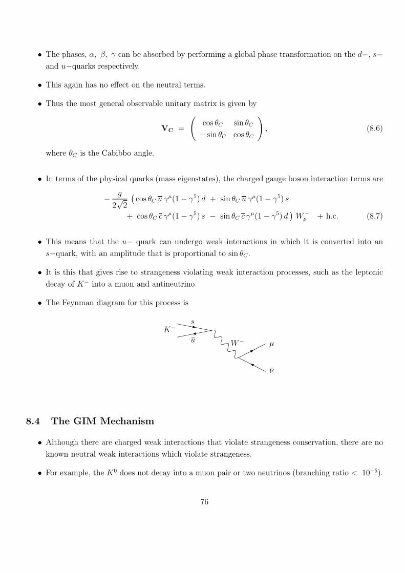
• The phases, α, β, γ can be absorbed by performing a global phase transformation on the d−, s−and u−quarks respectively.
• This again has no effect on the neutral terms.
• Thus the most general observable unitary matrix is given by
VC =
(cos θC sin θC
− sin θC cos θC
), (8.6)
where θC is the Cabibbo angle.
• In terms of the physical quarks (mass eigenstates), the charged gauge boson interaction terms are
− g
2√2
(cos θC u γ
µ(1− γ5) d + sin θC u γµ(1− γ5) s
+ cos θC c γµ(1− γ5) s − sin θC c γ
µ(1− γ5) d)W−µ + h.c. (8.7)
• This means that the u− quark can undergo weak interactions in which it is converted into an
s−quark, with an amplitude that is proportional to sin θC .
• It is this that gives rise to strangeness violating weak interaction processes, such as the leptonic
decay of K− into a muon and antineutrino.
• The Feynman diagram for this process is
K−s
u
ν
µW−
8.4 The GIM Mechanism
• Although there are charged weak interactions that violate strangeness conservation, there are no
known neutral weak interactions which violate strangeness.
• For example, the K0 does not decay into a muon pair or two neutrinos (branching ratio < 10−5).
76
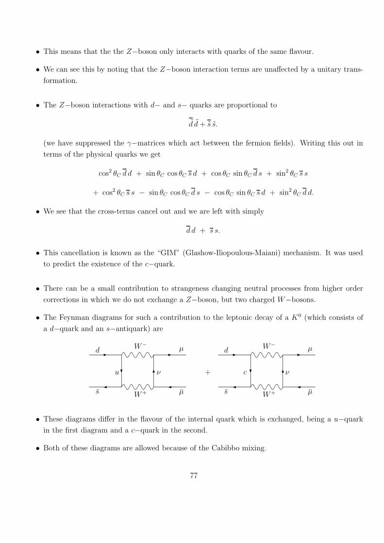
• This means that the the Z−boson only interacts with quarks of the same flavour.
• We can see this by noting that the Z−boson interaction terms are unaffected by a unitary trans-
formation.
• The Z−boson interactions with d− and s− quarks are proportional to
d d+ s s.
(we have suppressed the γ−matrices which act between the fermion fields). Writing this out in
terms of the physical quarks we get
cos2 θC d d + sin θC cos θC s d + cos θC sin θC d s + sin2 θC s s
+ cos2 θC s s − sin θC cos θC d s − cos θC sin θC s d + sin2 θC d d.
• We see that the cross-terms cancel out and we are left with simply
d d + s s.
• This cancellation is known as the “GIM” (Glashow-Iliopoulous-Maiani) mechanism. It was used
to predict the existence of the c−quark.
• There can be a small contribution to strangeness changing neutral processes from higher order
corrections in which we do not exchange a Z−boson, but two charged W−bosons.
• The Feynman diagrams for such a contribution to the leptonic decay of a K0 (which consists of
a d−quark and an s−antiquark) are
d
s
W−
W+
µ
µ
νu c+
d
s
W−
W+
µ
µ
ν
• These diagrams differ in the flavour of the internal quark which is exchanged, being a u−quark
in the first diagram and a c−quark in the second.
• Both of these diagrams are allowed because of the Cabibbo mixing.
77
• The first of these diagrams gives a contribution proportional to
+ sin θC cos θC ,
which arises from the product of the two couplings involving the emission of the W−bosons.
• The second diagram gives a term proportional to
− cos θC sin θC .
• If the c−quark and u−quark had identical mass then these two contributions would cancel pre-
cisely.
• However, the c−quark is much more massive than the u−quark, there is some residual contribu-
tion.
• This was used to limit the mass of the c−quark to < 5 GeV, before it was discovered.
8.5 Adding a Third Generation
• Adding a third generation is achieved in the same way.
• In this case the three weak isodoublets of left-handed fermions are(u
d
),
(c
s
),
(t
b
),
where d, s and b are related to the physical d−, s− and b−quarks by
d
s
b
= VCKM
d
s
b
. (8.8)
• The 3× 3 unitary matrix VCKM is the “Cabibbo-Kobayashi-Maskawa (CKM) matrix”.
• Once again it only affects the charged weak processes in which a W−boson is exchanged.
• For this reason the elements are written as
Vud Vus Vub
Vcd Vcs Vcb
Vtd Vts Vtb
78
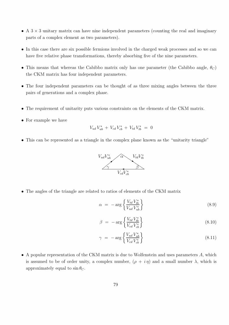
• A 3 × 3 unitary matrix can have nine independent parameters (counting the real and imaginary
parts of a complex element as two parameters).
• In this case there are six possible fermions involved in the charged weak processes and so we can
have five relative phase transformations, thereby absorbing five of the nine parameters.
• This means that whereas the Cabibbo matrix only has one parameter (the Cabibbo angle, θC)
the CKM matrix has four independent parameters.
• The four independent parameters can be thought of as three mixing angles between the three
pairs of generations and a complex phase.
• The requirement of unitarity puts various constraints on the elements of the CKM matrix.
• For example we have
Vud V∗ub + Vcd V
∗cb + Vtd V
∗tb = 0
• This can be represented as a triangle in the complex plane known as the “unitarity triangle”
VudV∗ub VtdV
∗tb
VcdV∗cb
α
βγ
• The angles of the triangle are related to ratios of elements of the CKM matrix
α = − arg
{Vtd V
∗tb
Vud V∗ub
}(8.9)
β = − arg
{Vtd V
∗tb
Vcd V∗cb
}(8.10)
γ = − arg
{Vud V
∗ub
Vcd V ∗cb
}(8.11)
• A popular representation of the CKM matrix is due to Wolfenstein and uses parameters A, which
is assumed to be of order unity, a complex number, (ρ + i η) and a small number λ, which is
approximately equal to sin θC .
79
• In terms of these parameters the CKM matrix is written
VCKM =
1− λ2/2 λ Aλ3 (ρ− i η)
−λ 1− λ2/2 Aλ2
Aλ3 (1− ρ− i η) −Aλ2 1
+ O(λ4). (8.12)
• We see that whereas the W−bosons can mediate a transition between a u−quark and a b−quark
(Vub) or between a t−quark and a d−quark (Vtd), the amplitude for such transitions are suppressed
as the cube of the small quantity which determines the amplitude for transitions between the first
and second generations, λ.
• The O(λ4) corrections are needed to ensure the unitarity of the CKM matrix and these corrections
have several matrix elements which are complex.
8.6 Mass generation - a summary
• Starting from the Yukawa interactions
L(q,e)Y = λuijqLiuRjH2 + λdijqLidRjH1 + λeijlLieRjH1 + h.c. , (8.13)
where H2 = iσ2H†1. Setting the vacuum expectation value of the Higgs fields as, 〈H1〉 = (0, v/
√2)T
L(q,e)M = muijuLiuRj +mdijdLidRj +meijeLieRj + h.c. , (8.14)
with the mass matrices for up-quarks, down-quarks and charged leptons,
mu = λuv√2, md = λd
v√2, me = λe
v√2. (8.15)
• The mass matrices are diagonalized by bi-unitary transformations,
V (u)†muV(u) = mdiag
u , V (d)†mdV(d) = mdiag
d , V (e)†meV(e) = mdiag
e , (8.16)
with V (u)†V (u) = 1, etc. , which also define the transition from mass eigenstates ψLα, ψRα to weak
eigenstates ψLi, ψRi,
uLi = V(u)iα uLα , dLi = V
(d)iα dLα , . . . , eRi = V
(e)iα eRα . (8.17)
• Since in general the transformation matrices are different for up- and down-quarks one obtains a
mixing between mass eigenstates in the charged current (CC) weak interactions,
L(q)EW = − g√
2
∑
i
uLiγµdLi W
+µ + . . . (8.18)
= − g√2
∑
α,β
uLαγµVαβdLβ W
+µ + . . . ,
where Vαβ = V(u)†αi V
(d)iβ is the familiar CKM mixing matrix.
80
• In general the Yukawa couplings are complex; hence, also the CKM matrix is complex, which
leads to CP violation in weak interactions.
• Without right-handed neutrinos, weak and mass eigenstates can always be chosen to coincide for
leptons.
• As a consequence, there is no mixing in the leptonic charged current,
L(l)EW = − g√
2
∑
α
eLiγµνLi W
−µ + . . . , (8.19)
and electron-, muon- and tau-number are separately conserved.
• On the contrary, in the quark sector only the total baryon number is conserved.
• We can write the full charged current interactions in terms of currents are
Lcc = − g√2
(J−µW
+µ + J+µW
−µ)
where
J+µ =
1
2uαVαβγµ(1− γ5)dβ +
1
2ναγµ(1− γ5)eα
and
J−µ =
1
2dαV
†αβγµ(1− γ5)uβ +
1
2eαγµ(1− γ5)να
• The neutral current interaction does not contain the CKM matrix and can be written in the form
Lnc =∑
fi
− g
2 cos θWfi(t3(fi) γ
µ (1− γ5)− 2Q(fi) sin2 θWγ
µ)fi Zµ −Q(fi) g sin θW fi γ
µ fiAµ
= − g
2 cos θWJ0µ Z
µ − g sin θW Jemµ Aµ
where
J0µ = J3
µ − sin2 θWJemµ
and
J3µ =
∑
fi
fi(t3(fi) γµ(1− γ5
))fi
and
Jemµ =
∑
fi
Q(fi) g sin θW fi γµ fi
81
• Often the neutral current is written
J0µ =
∑
fi
[gfiL f iLγµfiL + gfiRf iRγµfiR
]
=1
2
∑
fi
[gfiL f iγµ(1− γ5)fi + gfiRf iγµ(1 + γ5)fi
]
where
gfiL,R = t3(fi)−Q(fi) sin2 θW
• At low energies the effective action has the form
Leff = − g2
2M2W
J+µ J
−µ − g2
2 cos2 θWM2Z
J0µJ
0µ (8.20)
= − g2
2M2W
J+µ J
−µ − g2
2M2W
J0µJ
0µ
which can be compared with Fermi theory to get the value
GF =g2
4√2M2
W
as we did before.
8.7 CP Violation
• The possibility that some of the elements of the CKM matrix may be complex provides a mech-
anism for the violation of CP conservation.
• Violation of CP conservation has been observed in the K0, K0system, and is currently being
investigated for B−mesons.
• Higher order corrections to the masses of B0 and B0, give rise to mixing between the two states.
• Thus the mass matrix can be written(
MB0 ∆M
(∆M)∗ MB0
).
• The mass eigenstates are therefore
|BL〉 = p |B0〉 + q |B0〉, (8.21)
82
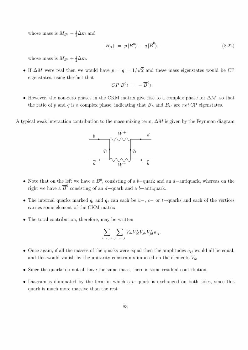
whose mass is MB0 − 12∆m and
|BH〉 = p |B0〉 − q |B0〉, (8.22)
whose mass is MB0 + 12∆m.
• If ∆M were real then we would have p = q = 1/√2 and these mass eigenstates would be CP
eigenstates, using the fact that
CP |B0〉 = −|B0〉.
• However, the non-zero phases in the CKM matrix give rise to a complex phase for ∆M , so that
the ratio of p and q is a complex phase, indicating that BL and BH are not CP eigenstates.
A typical weak interaction contribution to the mass-mixing term, ∆M is given by the Feynman diagram
b
d
W+
W−
d
b
qjqi
• Note that on the left we have a B0, consisting of a b−quark and an d−antiquark, whereas on the
right we have a B0consisting of an d−quark and a b−antiquark.
• The internal quarks marked qi and qj can each be u−, c− or t−quarks and each of the vertices
carries some element of the CKM matrix.
• The total contribution, therefore, may be written
∑
i=u,c,t
∑
j=u,c,t
Vib V∗id Vjb V
∗jd aij .
• Once again, if all the masses of the quarks were equal then the amplitudes aij would all be equal,
and this would vanish by the unitarity constraints imposed on the elements Vik.
• Since the quarks do not all have the same mass, there is some residual contribution.
• Diagram is dominated by the term in which a t−quark is exchanged on both sides, since this
quark is much more massive than the rest.
83
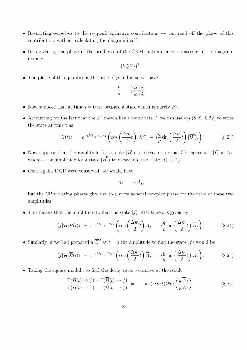
• Restricting ourselves to the t−quark exchange contribution, we can read off the phase of this
contribution, without calculating the diagram itself.
• It is given by the phase of the products, of the CKM matrix elements entering in the diagram,
namely
(V ∗td Vtb)
2.
• The phase of this quantity is the ratio of p and q, so we have
p
q=
V ∗td VtbVtd V ∗
tb
• Now suppose that at time t = 0 we prepare a state which is purely B0.
• Accounting for the fact that the B0 meson has a decay rate Γ, we can use eqs.(8.21, 8.22) to write
the state at time t as
|B(t)〉 = e−iMt e−Γt/2
(cos
(∆m
2t
)|B0〉 + i
q
psin
(∆m
2t
)|B0〉.
)(8.23)
• Now suppose that the amplitude for a state |B0〉 to decay into some CP eigenstate |f〉 is Af ,
whereas the amplitude for a state |B0〉 to decay into the state |f〉 is Af .
• Once again, if CP were conserved, we would have
Af = ±Af ,
but the CP violating phases give rise to a more general complex phase for the ratio of these two
amplitudes.
• This means that the amplitude to find the state |f〉 after time t is given by
〈f |H|B(t)〉 = e−iMt e−Γt/2
(cos
(∆m
2t
)Af + i
q
psin
(∆m
2t
)Af
). (8.24)
• Similarly, if we had prepared a B0at t = 0 the amplitude to find the state |f〉 would be
〈f |H|B(t)〉 = e−iMt e−Γt/2
(cos
(∆m
2t
)Af + i
p
qsin
(∆m
2t
)Af
). (8.25)
• Taking the square moduli, to find the decay rates we arrive at the result
Γ(B(t) → f)− Γ(B(t) → f)
Γ(B(t) → f) + Γ(B(t) → f)= − sin (∆mt)ℑm
(q
p
Af
Af
). (8.26)
84
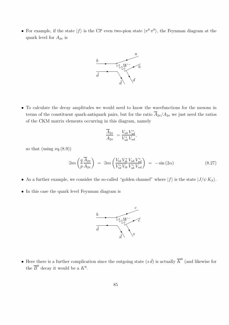
• For example, if the state |f〉 is the CP even two-pion state |π0 π0〉, the Feynman diagram at the
quark level for A2π is
W−b
d
u
u
dd
• To calculate the decay amplitudes we would need to know the wavefunctions for the mesons in
terms of the constituent quark-antiquark pairs, but for the ratio A2π/A2π we just need the ratios
of the CKM matrix elements occurring in this diagram, namely
A2π
A2π
=Vub V
∗ud
V ∗ub Vud
,
so that (using eq.(8.9))
ℑm(q
p
A2π
A2π
)= ℑm
(Vtd V
∗tb
V ∗td Vtb
Vub V∗ud
V ∗ub Vud
)= − sin (2α) (8.27)
• As a further example, we consider the so-called “golden channel” where |f〉 is the state |J/ψKS〉.
• In this case the quark level Feynman diagram is
W−b
d
c
c
sd
• Here there is a further complication since the outgoing state (s d) is actually K0(and likewise for
the B0decay it would be a K0.
85
• As in the B0 system, the mass eigenstates are given by
|KS〉 = pK |K0〉+ qK |K0〉
|KL〉 = pK |K0〉 − qK |K0〉.
• Once again, if CP were conserved we would have pK = qK = 1/√2, and these mass eigenstates
would be eigenstates of CP.
• The phases in the CKM matrix introduce a phase in the ratio of pK and qK , calculated from
diagrams similar to the ones for the B0 system (but with the b−quark replaced by an s−quark).
• In this case it is the diagram with internal c-quark exchange that dominates (although the mass of
thec− quark is much less than the t−quark the CKM matrix elements are much larger for c-quark
exchange than t−quark exchange and this effect dominates), so we have a factor
qKpK
=V ∗cd VcsVcd V ∗
cs
which enters in the ratio of the decay amplitudes, giving
AJ/ψKS
AJ/ψKS
= −Vcb V∗cs
V ∗cb Vcs
V ∗cd VcsVcd V ∗
cs
= −Vcb V∗cd
V ∗cb Vcd
,
(a minus occurs because the J/ψKS state is CP odd) so that (using eq.(8.10))
ℑm(q
p
AJ/ψKS
AJ/ψKS
)= −ℑm
(Vtd V
∗tb
V ∗td Vtb
Vcb V∗cd
V ∗cb Vcd
)= sin (2β) . (8.28)
8.8 Summary
• A left-handed quark doublet has weak hypercharge Y = 16, and the right-handed components have
weak hypercharges equal to the electric charges of the quarks themselves.
• In order to generate a mass for the T 3 = +12quark, one has to add a different type of Yukawa
coupling given by (8.4).
• A second generation may be added as a copy, but in this case one can have mass-mixing between
quarks of different generations. In terms of the mass eigenstates, the charged W−bosons mediate
transitions between a T 3 = +12quark (u or c) and a superposition of T 3 = −1
2quarks (d and
s). This mechanism allows weak interactions which violate strangeness conservation. The mixing
matrix has only one independent parameter, the Cabibbo angle.
86
• The GIM mechanism guarantees that there are no strangeness changing neutral processes. Weak
interactions involving the exchange of a Z−boson do not change flavour. There is a small violation
of this in higher orders owing to the mass splitting between the quarks.
• When one includes a third generation, the mixing matrix for the T 3 = −12quarks (d, s and b) is
the CKM matrix. This matrix has has four independent parameters, so that some of the matrix
elements may be complex.
• The possibility that some of the elements of the CKM matrix may be complex leads to a weak
interaction contribution to a mass mixing of B0 and B0which can be complex. This gives rise to
CP violation, since the eigenstates of the B0 mass matrix are then no longer also eigenstates of
CP . The CKM matrix also introduces phases in the ratios of the decay amplitudes for B0 and
B0to a given CP eigenstate. Products of the phase of the mass mixing and the ratio of the decay
amplitudes can be observed directly in tagged B−meson experiments and the angles α and β of
the unitarity triangle can be directly measured.
87
9 Neutrinos and the MNS matrix
9.1 Dirac Neutrino masses and mixings
• The simplest way to introduce
L(ν)Y = λνijlLiνRjH2 + h.c. (9.1)
• The Yukawa interaction defines the quantum numbers of the right-handed neutrino: it carries
lepton number, which is a global charge, but no colour, weak isospin or hypercharge
νR : (1, 1, 0)
• The Yukawa interaction which couples left-handed and right-handed neutrinos yields after spon-
taneous symmetry breaking the Dirac neutrino mass matrix
mD =λνv√2
• with v = 246 GeV we need
λν ∼ 10−13
such that
mD ∼ 0.01 eV
or smaller.
• Problem with this is that we must justify the size of λν .
9.2 Majorana Neutrinos and the see-saw mechanism
• A popular way to introduce neutrino masses is to allow the νRs to be majorana.
• This allows additional Yukawa couplings and a Majorana mass term,
L(ν)Y = λνijlLiνRjH2 +
1
2MijνcRiνRj + h.c. (9.2)
• A Majorana mass term is allowed for the right-handed neutrinos, consistent with the gauge sym-
metries of the theory.
• It is very important that these masses are not generated by the Higgs mechanism and can therefore
be much larger than ordinary quark and lepton masses.
88
• This leads to light neutrino masses via the seesaw mechanism.
• The Yukawa interaction which couples left-handed and right-handed neutrinos yields after spon-
taneous symmetry breaking the Dirac neutrino mass matrix mD = hνv/√2, the complete mass
terms are given by
L(ν)M = mDijνLiνRj +
1
2MijνcRiνRj + h.c. (9.3)
• We now wish to write the term as a mixing matrix (and its hermitian conjugate) to do so we need
the following
νLmDνR =1
2
(νLmDνR − νTRm
TDνL
T)
then using the following
νcL = C(νL)T → C−1νcL = (νL)
T
and νcL = −νTLC−1 → νcLC = −νTL
with
C = iγ2γ0 C† = C−1 CT = −C
using these identities we then have
−νTRmTDνL
T = νcRCmTDC
−1νcL = νcRmTDν
cL
the mass terms are then
L(ν)M =
1
2mDijνLiνRj +
1
2mTDijν
cRiν
cLj +
1
2MijνcRiνRj + h.c.
and can be written in matrix form
L(ν)M =
1
2
(νL νcR
)( 0 mD
mTD M
)(νcLνR
)+ h.c. (9.4)
• The unitary matrix which diagonalizes this mass matrix is easily constructed as power series in
ξ = mD/M . Up to terms O(ξ3) one obtains(νL
νcR
)=
(1− 1
2ξξ† ξ
−ξ† 1− 12ξξ†
)(L
Rc
). (9.5)
• In terms of the new left- and right-handed fields, L and R, the mass matrix is diagonal,
L(ν)M =
1
2
(L Rc
)( mν 0
0 M
)(Lc
R
)+ h.c. (9.6)
89
• Here the mass matrix mν is given by
mν = −mD1
MmTD . (9.7)
• This is the famous seesaw mass relation.
• With M ≫ mD, one obviously has mν ≪ mD.
• As an example, consider the case of just one generation.
• Choosing for mD the largest know fermion mass,
mD ∼ mt ∼ 100 GeV
and for M the unification scale of unified theories,
M ∼ 1015 GeV
one finds
mν ∼ 10−2 eV
which is precisely in the range of present experimental indications for neutrino masses.
• mν and M are the mass matrices of the light neutrinos and their heavy partners, respectively.
• The corresponding mass eigenstates are Majorana fermions,
ν = L+ Lc = νc , N = Rc +R = N c . (9.8)
• L,Rc and Lc, R are the corresponding left- and right-handed components,
L =1− γ5
2ν , Rc =
1− γ52
N , etc. (9.9)
• In terms of the Majorana fields the mass terms read,
L(ν)M =
1
2νmν
1 + γ52
ν +1
2Nmν
1 + γ52
N + h.c.
=1
2ν (Re{mν}+ iIm{mν}γ5) ν +
1
2N (Re{M} + iIm{M}γ5)N . (9.10)
• Note, that in general the mass matrices have real and imaginary parts. This is a consequence of
complex Yukawa couplings and a possible source of CP violation.
90
9.3 MNS matrix and Counting phases for Dirac and Majorana Neutrinos
• First let us recall in detail what happens for the quarks
• In the mass basis we have the following terms in the lagrangian
Lquarks = − g√2
∑
α,β
uLαγµVαβdLβ W
+µ +mdiag
u (uLuR + uRuL) +mdiagd (dLdR + dRdL) + . . . ,
• The CKM matrix is a 3X3 Unitary matrix.
• A general unitary matrix has 9 real parameters
• We can remove phases be performing field redefintions
• We have 6 fields and so we can remove 5 parameters leaving 4 real parameters: 3 angles and 1
phase
Now Dirac Neutrinos
• Neutrino masses imply mixing in the leptonic charged current.
• Counting is the same as for quarks
• Lagrangian mass terms are:
Lleptonmass = mDijνLνR +meijeLieRj + h.c. , (9.11)
• The mass mixing matrices are diagonalised by the following
V (ν)†mDV(ν) = mdiag
ν , (9.12)
V (e)†meV(e) = mdiag
e ,
• with the mass and weak eigenstates related as
νLi = V(ν)iα uLα , νRi = V
(ν)iα νRα , eLi = V
(e)iα eLα , eRi = V
(e)iα eRα .
• The resulting weak interaction terms in the mass eigenstate basis
Lleptonmass = − g√2
∑
α,β
νLαγµV mns
αβ eLβ W+µ +mdiag
ν (νLνR + νRνL) +mdiage (eLeR + eReL) + . . . ,
where
V mnsαβ = V
(ν)†αi V
(e)iβ
91
• We can do the same counting as with the CKM matrix:
• We have can perform 6 field redefinitions removing 5 parameter leaving 4: 3 angles and a phase
• Note: due to the mixing e-, µ- and τ -number are now no longer separately conserved.
Now Majorana Neutrinos
• The Majorana mass terms from before are
L(ν)M = νmνν +NMN . (9.13)
• Forget the heavy neutrinos
• If the neutrino mass matrix is diagonalized by the unitary matrix U (ν),
U (ν)†mνU(ν)∗ = −
m1 0 0
0 m2 0
0 0 m3
, (9.14)
the mixing matrix U appears in the charged current,
L(l)EW = −− g√
2
∑
α,β
νLαγµUmns
αβ eLβ W+µ + νmνν +NMN + . . . , (9.15)
where
Umnsij = U
(ν)†iα V
(e)αj . (9.16)
again e-, µ- and τ -number are now no longer separately conserved.
• This time the counting is different.
• We do not have the same freedom as we did before to make field redefinitions due to the Majorana
nature of the neutrinos.
• We can rewrite the Majorana mass terms as follow
νmνν = −νTC−1mνν
• If for example we make a phase redefinition of one of the neutrinos fields, the mass term will
change and pick up a phase
• This means that we can remove fewer parameters from the MNS matrix meaning we have more
physical parameters.
92
• Turns out the result is that you can remove 2 less phases
• In Majorana neutrino case the MNS matrix we have 3 angles and 3 phases.
• 2 extra phases are often referred to as Majorana phases
93
10 Anomalies
• So far, we have taken the hypercharge assignments of our fermion fields but at the classical level
the assignments are arbitrary.
• However, at the quantum level this is not true.
• The Adler-Bell-Jackiw anomaly spoils the renormalisabilty of the theory whenever it spoils the
conservation of a gauged current
• Adler-Bardeen theorem asserts that the anomaly occurs only at one loop order.
⇒ Only need to make sure the relevant one loop diagrams vanish to leave the theory renormalisable
• This restricts the hypercharge assignments (and also the particle content of the theory)
• We also find that there is an anomaly associated with the chiral symmetry and we start by
analysing this.
Axial Current and triangle diagrams
• For massless fermions, the 4d Dirac equation splits into separate terms for left and right handed
fermions
• Introducing gauge field we replace derivatives by covariant derivatives
→ does not affect this separation
• This should mean that the vector and axial vector currents remain conserved
BUT this is not the case for the axial current after we include quantum effects
• Without the quantum effects we have
jµ(x) = ψ(x)γµψ(x) jµ5(x) = ψ(x)γµγ5ψ(x)
∂µjµ = 0, ∂µj
µ5 = 0
in the limit of zero quark masses and we are considering the following symmetry transformations
ψ(x) → eiαψ ψ(x) → eiαγ5ψ
for vector and axial symmetries
What happens in the quantum case, start with QED Lagrangian with one massless
fermion
L = ψ(i/D)ψ − 1
4(Fµν)
2
94
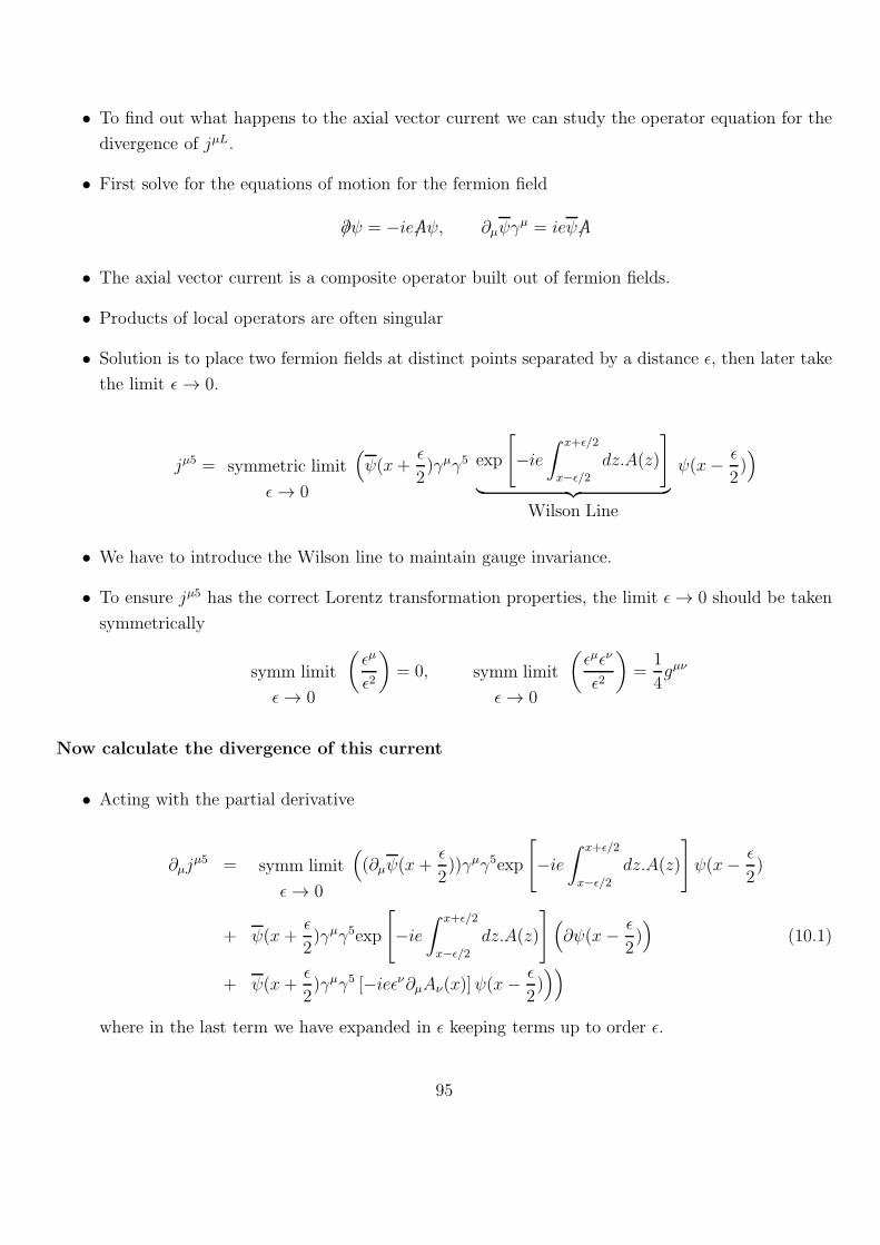
• To find out what happens to the axial vector current we can study the operator equation for the
divergence of jµL.
• First solve for the equations of motion for the fermion field
/∂ψ = −ie/Aψ, ∂µψγµ = ieψ/A
• The axial vector current is a composite operator built out of fermion fields.
• Products of local operators are often singular
• Solution is to place two fermion fields at distinct points separated by a distance ǫ, then later take
the limit ǫ → 0.
jµ5 = symmetric limit
ǫ→ 0
(ψ(x+
ǫ
2)γµγ5 exp
[−ie
∫ x+ǫ/2
x−ǫ/2dz.A(z)
]
︸ ︷︷ ︸Wilson Line
ψ(x− ǫ
2))
• We have to introduce the Wilson line to maintain gauge invariance.
• To ensure jµ5 has the correct Lorentz transformation properties, the limit ǫ→ 0 should be taken
symmetrically
symm limit
ǫ→ 0
(ǫµ
ǫ2
)= 0, symm limit
ǫ→ 0
(ǫµǫν
ǫ2
)=
1
4gµν
Now calculate the divergence of this current
• Acting with the partial derivative
∂µjµ5 = symm limit
ǫ→ 0
((∂µψ(x+
ǫ
2))γµγ5exp
[−ie
∫ x+ǫ/2
x−ǫ/2dz.A(z)
]ψ(x− ǫ
2)
+ ψ(x+ǫ
2)γµγ5exp
[−ie
∫ x+ǫ/2
x−ǫ/2dz.A(z)
] (∂ψ(x − ǫ
2))
(10.1)
+ ψ(x+ǫ
2)γµγ5 [−ieǫν∂µAν(x)]ψ(x−
ǫ
2)))
where in the last term we have expanded in ǫ keeping terms up to order ǫ.
95
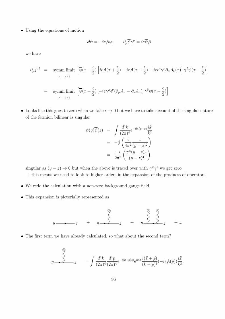
• Using the equations of motion
/∂ψ = −ie/Aψ, ∂µψγµ = ieψ/A
we have
∂µjµ5 = symm limit
ǫ → 0
[ψ(x+
ǫ
2)[ie/A(x+
ǫ
2)− ie/A(x− ǫ
2)− ieǫνγµ∂µAν(x)
]γ5ψ(x− ǫ
2)]
= symm limit
ǫ → 0
[ψ(x+
ǫ
2) [−ieγµǫν(∂µAν − ∂νAµ)] γ
5ψ(x− ǫ
2)]
• Looks like this goes to zero when we take ǫ→ 0 but we have to take account of the singular nature
of the fermion bilinear is singular
ψ(y)ψ(z) =
∫d4k
(2π)4e−ik.(y−z)
i/k
k2
= −/∂(
i
4π2
1
(y − z)2
)
=−i2π2
(γα(y − z)α(y − z)4
).
singular as (y − z) → 0 but when the above is traced over with γµγ5 we get zero
→ this means we need to look to higher orders in the expansion of the products of operators.
• We redo the calculation with a non-zero background gauge field
• This expansion is pictorially represented as
y z + y z
⊗
+ y z
⊗ ⊗
+ ...
• The first term we have already calculated, so what about the second term?
y z
⊗
=
∫d4k
(2π)4d4p
(2π)4e−i(k+p).yeik.z
i(/k + /p)
(k + p)2(−ie/A(p)) i/k
k2.
96
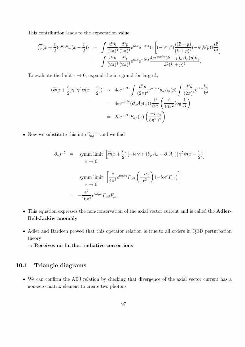
This contribution leads to the expectation value
〈ψ(x+ ǫ
2)γµγ5ψ(x− ǫ
2)〉 =
∫d4k
(2π)4d4p
(2π)4eik.ǫe−ip.xtr
[(−γµγ5) i(/k + /p)
(k + p)2(−ie/A(p)) i/k
k2
]
=
∫d4k
(2π)4d4p
(2π)4eik.ǫe−ip.x
4eǫµαβγ(k + p)αAβ(p)kγk2(k + p)2
.
To evaluate the limit ǫ→ 0, expand the integrand for large k,
〈ψ(x+ ǫ
2)γµγ5ψ(x− ǫ
2)〉 ∼ 4eǫµαβγ
∫d4p
(2π)4e−ip.xpαAβ(p)
∫d4k
(2π)4eik.ǫ
kγk4
= 4eǫµαβγ(∂αAβ(x))∂
∂ǫγ
(i
16π2log
1
ǫ2
)
= 2eǫµαβγFαβ(x)
( −i8π2
ǫγǫ2
)
• Now we substitute this into ∂µjµ5 and we find
∂µjµ5 = symm limit
ǫ→ 0
[ψ(x+
ǫ
2) [−ieγµǫν(∂µAν − ∂νAµ)] γ
5ψ(x− ǫ
2)]
= symm limit
ǫ→ 0
[e
4π2ǫµαβγFαβ
(−iǫγǫ2
)(−ieǫνFµν)
]
= − e2
16π2ǫαβµνFαβFµν .
• This equation expresses the non-conservation of the axial vector current and is called the Adler-
Bell-Jackiw anomaly
• Adler and Bardeen proved that this operator relation is true to all orders in QED perturbation
theory
→ Receives no further radiative corrections
10.1 Triangle diagrams
• We can confirm the ABJ relation by checking that divergence of the axial vector current has a
non-zero matrix element to create two photons
97
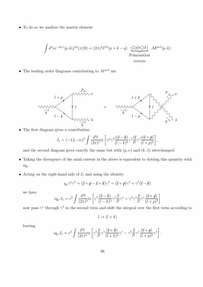
• To do so we analyze the matrix element
∫d4xe−iq.x〈p, k|jµ5(x)|0〉 = (2π)4δ(4)(p + k − q) ǫ∗ν(p)ǫ
∗λ(k)︸ ︷︷ ︸
Polarisation
vectors
Mµνλ(p, k)
• The leading order diagrams contributing to Mµνλ are
q−→
p−→
k−→
l + p
l − k
l
λ
ν
+
q−→
pր
kց
l + k
l − p
l
λ
ν
• The first diagram gives a contribution
I1 = (−1)(−ie)2∫
d4l
(2π)4tr
[γµγ5
i(/l − /k)
(l − k)2γλi/l
l2γνi(/l + /p)
(l + p)2
],
and the second diagram gives exactly the same but with (p, ν) and (k, λ) interchanged.
• Taking the divergence of the axial current in the above is equivalent to dotting this quantity with
iqµ.
• Acting on the right-hand side of I1 and using the identity
qµγµγ5 = (/l + /p− /l + /k)γ5 = (/l + /p)γ5 + γ5(/l − /k)
we have
iqµ.I1 = e2∫
d4l
(2π)4tr
[γ5
(/l − /k)
(l − k)2γλ
/l
l2γν + γ5γλ
/l
l2γν
(/l + /p)
(l + p)2
]
now pass γν through γ5 in the second term and shift the integral over the first term according to
l → (l + k)
leaving
iqµ.I1 = e2∫
d4l
(2π)4tr
[γ5
/l
l2γλ
(/l + /k)
(l + k)2γν − γ5
/l
l2γν
(/l + /p)
(l + p)2γλ].
98
• This expression is manifestly antisymmetric under the interchange of (p, ν) and (k, λ), so the
contribution from the second diagram cancels this.
However
• Because this derivation involves a shift of the integration variable, we have to be careful about
whether this shift is allowed by the regularisation
• These integrals are divergent.
• If we use a momentum cut-off, or Pauli-Villars regularisation it turns out that the shift leaves
over a finite, non-zero term.
• This is similar to the analysis of QED vacuum polarisation which is fixed by dimensional regular-
isation.
• For the axial vector current even dimensional regularisation contains a subtlety.
• It is due to the fact that γ5 is intrinsically 4-dimensional. (In dim reg we use extra dimensions to
regularise the integrals.)
• ’t Hooft and Veltman in their original paper defined
γ5 = iγ0γ1γ2γ3
in d- dimensions.
• Consequence of this is that
γ5 anticommuteswith γµ forµ = 0, 1, 2, 3
and
γ5 commuteswith γµ for µ = others
• In evaluating the integral in dim reg the momentum p, k and q all live in 4-d but the loop
momentum l has components in all dimensions.
• Write
l = l‖ + l⊥,
where the first term has nonzero components in dimensions 0, 1, 2, 3 and the second terms has
nonzero components in the other d− 4 dimensions.
99
• Due to the commutation relations for γ5 the identity for qµγµγ5 is now
qµγµγ5 = (/l + /k)γ5 + γ5(/l − /p)− 2γ5/l⊥
• First two terms cancel as before, but the third term give the additional contribution
iqµ.I1 = e2∫
d4l
(2π)4tr
[−2γ5/l⊥
(/l − /k)
(l − k)2γλ
/l
l2γν
(/l + /p)
(l + p)2
]
• To evaluate this we combine denominators and shift the integration variables
l → l + P
where
P = xk − yp
• After some manipulation we have to evaluate the integral
∫d4l
(2π)4/l⊥/l⊥
(l2 −∆)3
where
∆ = ∆(k, p, x, y)
using
(/l⊥)2 = l2⊥ → (d− 4)
dl2
under the integration the integral can be written as
i
(4π)d/2(d− 4)
2
Γ(2− d2)
Γ(3)∆2−d/2 −→d → 4
−i2(4π)2
• Notice that the integral which seems to have a logarithmic divergence is finite using dim reg
• The remainder of the calculation is fairly straightforward. The terms involving the momentum
shift P cancel and we find
iqµ.I1 = e2( −i2(4π)2
)tr[2γ5(−/k)γλ/pγν
]
=e2
4π2ǫαλβνkαpβ
100
• This is symmetric under interchange of (p, ν) and (k, λ) so the second diagram gives an identical
contribution.
• Thus:
〈p, k|∂µjµ5(x)|0〉 =−e22π2
ǫαλβν(−ipα)ǫ∗ν(p)(−ikβ)ep∗λ(k)
=−e22π2
〈p, k|ǫαλβνFανFβλ(0)|0〉
Which is the same as the ABJ anomaly equation.
10.2 Chiral Anomalies and Chiral Gauge Theories
• Up to now we have coupled gauge fields to fermions in a parity symmetric way
• That is we have replaced the derivative in the Dirac equation with a covariant derivative
• This means that the gauge fields couple to the vector current of fermions
• This only gives a subset of the possible couplings
• Now we will construct parity-asymmetric couplings and discuss their interplay with the axial
current
First consider massless fermions
• No mass terms means no mixing between the LH and RH components of our Dirac fermions
• Thus in this theory we can write the kinetic energy terms in terms of Weyl Spinors
L = ψ†Liiσ.∂ψLi + ψ†
Riiσ.∂ψRi
• We are free to couple this system to a gauge field by assigning the LH fields to one representation,
say r of G and the RH to another.
• Let us say that they do not transform under G.
• Doing so we adapt the derivatives as normal to give
L = ψ†Liiσ.DψLi + ψ†
Riiσ.∂ψRi
with Dµ = ∂µ − igAaµTar
101
• We can write this in terms of more traditional Dirac spinors as
L = ψiiγµ
(∂µ − igAaµT
ar
(1− γ5
2
))ψi
• The classical Lagrangian is invariant under
ψ →(1 + iαaT ar
(1− γ5
2
))ψ
Aaµ → Aaµ +1
g∂µα
a + fabcAbµαc
• The concept of only LH fields coupling to gauge fields is familiar to us through the weak interac-
tions
• A useful feature of chirally coupled fermions is that we can write RH fields as LH fields by writing
σ2ψ∗R
which transforms as a LH field under the Lorentz transformations
• This allows us to write the entire Lagrangian in terms of ”LH” fields.
• Define these new LH fields as
ψ′L = σ2ψ∗
R, ψ′†L = ψTRσ
2
• This relabels the RH fermions as antifermions and calls their LH antiparticles a new species of
LH fermion
• We can thus rewrite the Lagrangian for RH fields as (using integration by parts)∫d4xψ†
Riiσ.∂ψRi =
∫d4xψ′†
Liiσ.∂ψ′Li
• Notice that if these (originally RH) fermions transformed in rep r this manipulation changes the
way they transform
• Their covariant derivative will now be
ψ†Riσ.(∂ − igAaT ar )ψR = ψ′†
L iσ.(∂ + igAa(T ar )T )ψ′
L
= ψ′†L iσ.(∂ − igAaT ar )ψ
′L
Using
T ar = −(T ar )∗ = −(T ar )
T
102
• Thus the new fields transform as the conjugate representation to r.
Example: QCD
• nf flavours of massless fermions
• This theory describes a gauge theory coupled to nf massless fermions in the 3 and nf flavours in
the 3 representation of SU(3)
• The most general gauge theory of massless fermions would simply assign the LH fermions to an
arbitrary reducible representation R of the gauge group G
• We have just seen that rewriting the system of dirac fermions leads to R = r⊕ r as real represen-
tation.
• A real representation is such that there exists a unitary transformation U
T aR= UT aRU
†
• Conversely if R is not a real representation, then the theory cannot be written in terms of Dirac
fermions and is intrinsically chiral
• The mass terms for our QCD example are written as
mψiψi = m(ψ†RψL + h.c.) = −m(ψ′T
Liσ2ψLi + h.c.)
• This has the form of a Majorana mass term.
• Given this the most general mass term that can be built purely from LH fermion fields is
∆LM =MijψTLiσ
2ψLj + h.c.
this term is symmetric under exchange of i and j.
• This term is gauge invariant under G.
• In general, we can always write down a mass term if the representation containing the fermions
is strictly real.
• In an intrinsically chiral theory there is no possible invariant mass term
• At the classical level there is no restriction on the representation R of the LH fermions.
103
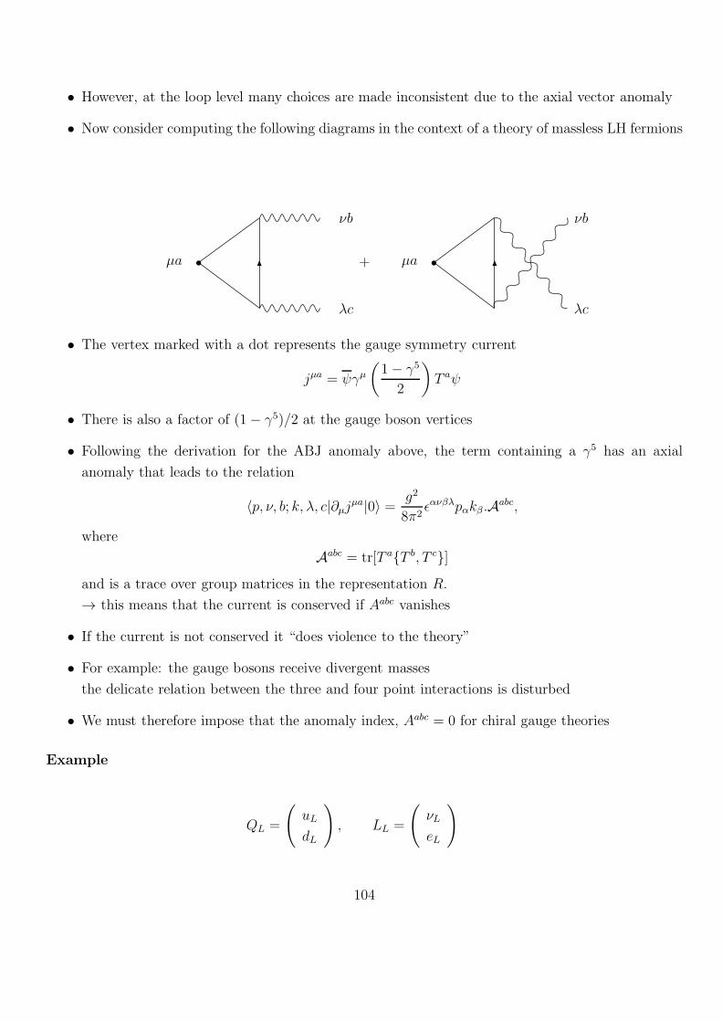
• However, at the loop level many choices are made inconsistent due to the axial vector anomaly
• Now consider computing the following diagrams in the context of a theory of massless LH fermions
µa
νb
λc
+ µa
νb
λc
• The vertex marked with a dot represents the gauge symmetry current
jµa = ψγµ(1− γ5
2
)T aψ
• There is also a factor of (1− γ5)/2 at the gauge boson vertices
• Following the derivation for the ABJ anomaly above, the term containing a γ5 has an axial
anomaly that leads to the relation
〈p, ν, b; k, λ, c|∂µjµa|0〉 =g2
8π2ǫανβλpαkβ.Aabc,
where
Aabc = tr[T a{T b, T c}]and is a trace over group matrices in the representation R.
→ this means that the current is conserved if Aabc vanishes
• If the current is not conserved it “does violence to the theory”
• For example: the gauge bosons receive divergent masses
the delicate relation between the three and four point interactions is disturbed
• We must therefore impose that the anomaly index, Aabc = 0 for chiral gauge theories
Example
QL =
(uL
dL
), LL =
(νL
eL
)
104

• If the two gauge bosons in the anomaly diagrams are SU(2)L gauge bosons and the current is an
SU(2)L gauge current then by using
T a =σa
2
and
{σb, σc} = 2δbc
this gives
Aabc =1
8Tr[σa2δbc] = 0
so this anomaly is zero
• If QL and LL couple to the EM field there is an additional consistency condition found by the
taking the current to be EM
⇒ Aabc = Tr[Q{T b, T c}] = 1
2Tr(Q)δbc
where Q is the matrix of electric charges of the fermions
• Tr(Q) is thus the sum of the fermion electric charges
• For our example we have (remembering the factor of 3 for colour)
Tr(Q) = 3(2
3− 1
3) + (0− 1) = 0
• We see straight away that SU(2) weak interactions can be combined with QED only if the theory
contains equal numbers of quark and lepton doublets
Now more generally
• If the fermion representation R is real, R is equivalent to its conjugate representation R.
• From previously we had that for real reps TR is related by a unitary transformation to T aR
=
−(T aR)T .
• Since the anomaly coefficient is invariant under unitary transformations we can simply replace TR
by T aRthen
Aabc = Tr[(−T a)T{(−T b)T , (−T c)T}] = −Tr[{T b, T c}T a] = −Aabc
which means that the anomaly coefficient must be zero and therefore for any real representation
the gauge theory will be automatically anomaly free
105
In general circumstances...
• We simplify the calculation of A by noting that it is an invariant of the gauge group G that is
totally symmetric with three indices in the adjoint representation.
• For some possible groups a suitable invariant may not exist and in those cases Aabc vanishes.
Example: SU(2)
• The adjoint representation has spin 1
• The symmetric product of two spin 1 multiplets give a spin 0 and spin 2, with no spin 1
component.
• This means that there is no symmetric tensor coupling two spin 1 indices to give a spin 1
• Aabc in this case must therefore vanish in any SU(2) gauge theory - as we showed explicitly above
SU(N) with N ≥ 3
• There is a unique symmetric invariant dabc of the required type
• It appears in the anti-commutator of the representation matrices of the fundamental representation
{T aF , T bF} =1
nδab + dabcT cF
• The uniqueness of this invariant implies that, in an SU(N) gauge theory,any form of the trace of
the form Aabc = tr[T a{T b, T c}] is proportional to dabc.
• For each representation r, we can define an anomaly coefficient A(r) by
Tr[T ar {T br , T cr }] =1
2A(r)dabc
• For the fundamental representation, it is clear that
A(F ) = 1.
• It follows also that
A(r) = −A(r)
106
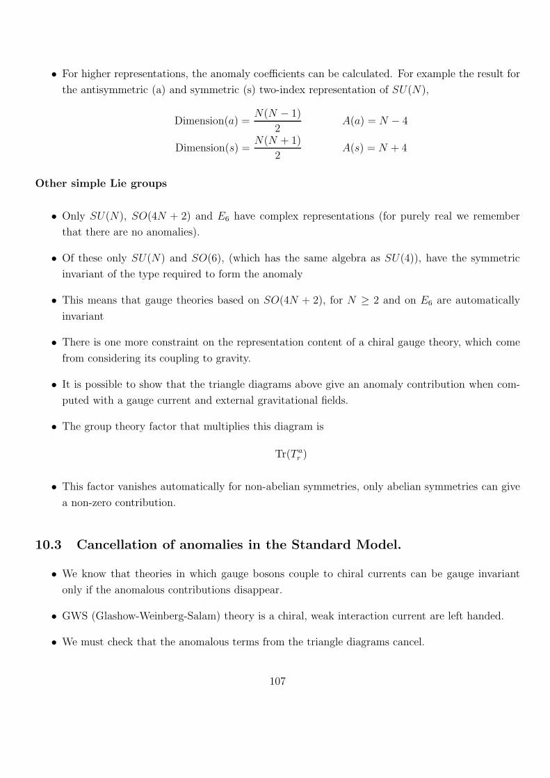
• For higher representations, the anomaly coefficients can be calculated. For example the result for
the antisymmetric (a) and symmetric (s) two-index representation of SU(N),
Dimension(a) =N(N − 1)
2A(a) = N − 4
Dimension(s) =N(N + 1)
2A(s) = N + 4
Other simple Lie groups
• Only SU(N), SO(4N + 2) and E6 have complex representations (for purely real we remember
that there are no anomalies).
• Of these only SU(N) and SO(6), (which has the same algebra as SU(4)), have the symmetric
invariant of the type required to form the anomaly
• This means that gauge theories based on SO(4N + 2), for N ≥ 2 and on E6 are automatically
invariant
• There is one more constraint on the representation content of a chiral gauge theory, which come
from considering its coupling to gravity.
• It is possible to show that the triangle diagrams above give an anomaly contribution when com-
puted with a gauge current and external gravitational fields.
• The group theory factor that multiplies this diagram is
Tr(T ar )
• This factor vanishes automatically for non-abelian symmetries, only abelian symmetries can give
a non-zero contribution.
10.3 Cancellation of anomalies in the Standard Model.
• We know that theories in which gauge bosons couple to chiral currents can be gauge invariant
only if the anomalous contributions disappear.
• GWS (Glashow-Weinberg-Salam) theory is a chiral, weak interaction current are left handed.
• We must check that the anomalous terms from the triangle diagrams cancel.
107
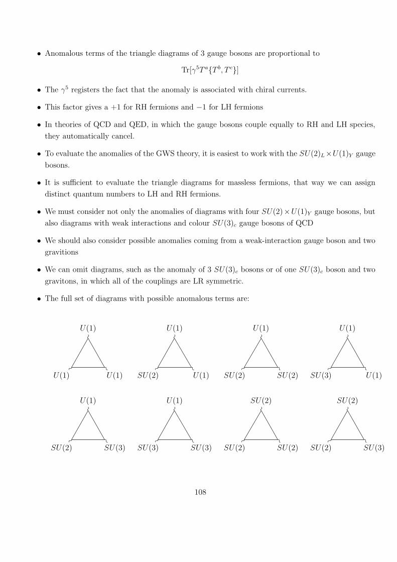
• Anomalous terms of the triangle diagrams of 3 gauge bosons are proportional to
Tr[γ5T a{T b, T c}]
• The γ5 registers the fact that the anomaly is associated with chiral currents.
• This factor gives a +1 for RH fermions and −1 for LH fermions
• In theories of QCD and QED, in which the gauge bosons couple equally to RH and LH species,
they automatically cancel.
• To evaluate the anomalies of the GWS theory, it is easiest to work with the SU(2)L×U(1)Y gauge
bosons.
• It is sufficient to evaluate the triangle diagrams for massless fermions, that way we can assign
distinct quantum numbers to LH and RH fermions.
• We must consider not only the anomalies of diagrams with four SU(2)×U(1)Y gauge bosons, but
also diagrams with weak interactions and colour SU(3)c gauge bosons of QCD
• We should also consider possible anomalies coming from a weak-interaction gauge boson and two
gravitions
• We can omit diagrams, such as the anomaly of 3 SU(3)c bosons or of one SU(3)c boson and two
gravitons, in which all of the couplings are LR symmetric.
• The full set of diagrams with possible anomalous terms are:
U(1)
U(1)U(1)
U(1)
U(1)SU(2)
U(1)
SU(2)SU(2)
U(1)
U(1)SU(3)
U(1)
SU(3)SU(2)
U(1)
SU(3)SU(3)
SU(2)
SU(2)SU(2)
SU(2)
SU(3)SU(2)
108
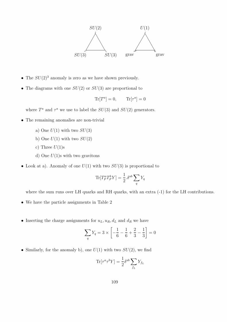
SU(2)
SU(3)SU(3)
U(1)
gravgrav
• The SU(2)3 anomaly is zero as we have shown previously.
• The diagrams with one SU(2) or SU(3) are proportional to
Tr[T a] = 0, Tr[τa] = 0
where T a and τa we use to label the SU(3) and SU(2) generators.
• The remaining anomalies are non-trivial
a) One U(1) with two SU(3)
b) One U(1) with two SU(2)
c) Three U(1)s
d) One U(1)s with two gravitons
• Look at a). Anomaly of one U(1) with two SU(3) is proportional to
Tr[T aFTbFY ] =
1
2.δab
∑
q
Yq
where the sum runs over LH quarks and RH quarks, with an extra (-1) for the LH contributions.
• We have the particle assignments in Table 2
• Inserting the charge assignments for uL, uR, dL and dR we have
∑
q
Yq = 3×[−1
6− 1
6+
2
3− 1
3
]= 0
• Similarly, for the anomaly b), one U(1) with two SU(2), we find
Tr[τaτ bY ] =1
2δab∑
fL
YfL
109
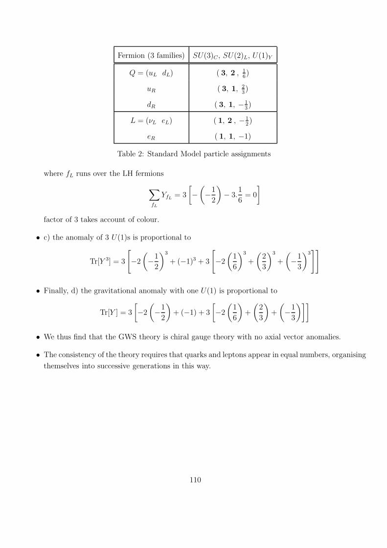
Fermion (3 families) SU(3)C , SU(2)L, U(1)Y
Q = (uL dL) ( 3, 2 , 16)
uR ( 3, 1, 23)
dR ( 3, 1, −13)
L = (νL eL) ( 1, 2 , −12)
eR ( 1, 1, −1)
Table 2: Standard Model particle assignments
where fL runs over the LH fermions
∑
fL
YfL = 3
[−(−1
2
)− 3.
1
6= 0
]
factor of 3 takes account of colour.
• c) the anomaly of 3 U(1)s is proportional to
Tr[Y 3] = 3
[−2
(−1
2
)3
+ (−1)3 + 3
[−2
(1
6
)3
+
(2
3
)3
+
(−1
3
)3]]
• Finally, d) the gravitational anomaly with one U(1) is proportional to
Tr[Y ] = 3
[−2
(−1
2
)+ (−1) + 3
[−2
(1
6
)+
(2
3
)+
(−1
3
)]]
• We thus find that the GWS theory is chiral gauge theory with no axial vector anomalies.
• The consistency of the theory requires that quarks and leptons appear in equal numbers, organising
themselves into successive generations in this way.
110
11 Chiral Lagrangian approximation
• We know αQCD becomes large at small energies.
• Do not expect that QCD can be described in terms of quarks and gluons
• The ”confinement hypothesis” asserts that only objects which are colour singlets may be identified
with free particles
• As we have seen before it is easy to construct combinations of quarks into colour singlets
qq : 3⊗ 3 = 1⊕ 8
and the totally antisymmetric combination of three quarks
qqq : (3⊗ 3⊗ 3)A = 1
• QCD also has colourless combinations of gluons - glue-balls
• Symmetric combinations of gluons
(8⊗ 8)S = 1⊕ ...
and
(8⊗ 8⊗ 8)S = 1⊕ ...
• These states are hard to find as they do not have electromagnetic interactions
• Mesons and Baryons are not of course as simple as this they are a mess of quark-antiquark pairs
and glue i.e. schematically
mesons : |qiqj(1 + qkqk + glue + ...)〉, (11.1)
baryons : |qiqjqk(1 + qlql + glue + ...)〉, (11.2)
• i, j, k, l are flavour indices, colour indices not shown but contracted in appropriate way to give
colour singlet.
• Should be noted that any colourless combinations is actually a linear superposition of all possible
colour singlets with the same quantum numbers
• Although the confinement hypothesis is consistent with experiment it is yet to be proven from
first principles
111
• Solution lies in developments in non-perturbative field theory
How best can we relate QCD to the ”nuclear force”? E.g. in π −N scattering?
• The key is to understand that the electroweak quantum numbers shared by quarks (and their
composites) allow us to see that the QCD lagrangian is spontaneously broken (presumably by the
QCD force itself) whilst leaving QCD unbroken
• Opens up a way of describing the static limit of QCD
First let us be clear about what we are describing.
• QCD is the fundamental theory of strong interactions
• The two phases:
quark-gluon phase at short distances
baryon-meson phase at long distances
are different phases of the same theory
• The intrinsic scale associated with QCD, ΛQCD provides a quantitative way to differentiate be-
tween the two phases
• E.g. quark masses can be put into two categories:
mq ≫ ΛQCD - quark can be viewed as quasi-free
mq ≪ ΛQCD - quark is strongly interacting
• Two phases share some symmetries (e.g. charge invariance) others can be treated differently
• In quark-gluon plasma some symmetries are linearly realised where as
in the baryon-meson phase are realised non-linearly (more later)
• Although we do not have the tools to derive the meson-baryon phase from first principals we can
use the symmetries to gain valuable information
Setting up the analysis:
112
• Turn off electroweak interactions
• Consider QCD interactions with non-zero quark masses
• Segregate quark masses according to relative sizes to ΛQCD:
mu, md ≪ ΛQCD
ms ∼ ΛQCD
mc, mb, mt ≫ ΛQCD
with c, b and t playing no part in the meson-baryon phases, i.e. large distance description of QCD.
• To start set mu = md = ms = 0 ⇒ the chiral limit
• QCD lagrangian is then (in terms of the Dirac q field)
LQCD = −1
4Tr(GµνG
µν) +
3∑
i=1
qiγµDµqi (11.3)
• By setting the masses to zero, we have gained a very large global symmetry:
SU(3)L × SU(3)R × U(1)
• This global symmetry is linearly realised on the three light quarks, u, d, s
SU(3)L : qL → ULqL; SU(3)R : qR → URqR;
U(1) : qL,R → eiαqL,R
this U(1) is actually baryon number
• There is also a flavour blind chiral U(1)
qL → eiβqL; qR → e−iβqR
but this symmetry is not conserved due to quantum effects (an anomaly) see later
• Above is in the quark phase, what happens in the baryon-meson phase
– Lorentz invariance is unbroken
– Colour invariance is unbroken
– Chiral symmetries of massless QCD are spontaneously broken
113
– Vector symmetries of massless QCD is unbroken
• These are all assumptions but the first two can be argued to be justifiable through experimental
observations
• The second two have important consequences
• If true the chiral symmetry is broken to its maximal vectorial subgroup
SU(3)L × SU(3)R → SU(3)v
leaving the U(1) unaffected.
What is responsible for the spontaneous symmetry breaking?
• Believed to take place through the condensation of quark pairs in the vacuum
• We don’t actually need to know how this happens as we ca infer consequences via symmetry
considerations
• Consider the fermion bi-linear of a quark and an anti-quark:
q†iaLαq
βRjb
where i and j are the SU(3)L and SU(3)R indices, α, β Lorentz indices, a, b are colour indices
• Under Lorentz the bilinear has the structure
(2, 1)⊗ (2, 1) ∼ (1, 1)⊕ (3, 1)
• Singlet combination means we do not break Lorentz invariance
• Similarly, under the colour group we have
3c ⊗ 3c = 1c ⊕ 8c
• Presence of a singlet means that this particular combination does not break colour.
What about the global symmetries?
• The SU(3)L × SU(3)R the bilinear transforms as (3, 3)
114
• This representations breaks up in terms of the diagonal vector-like subgroup SU(3)v as
(3, 3) → 1⊕ 8;
showing one component that breaks the chiral symmetry while preserving the vectorial subgroup
• It then follows that the bilinear achieves the desired effect:
The condensation of the bilinear breaks the chiral symmetry to the vectorial symme-
try whilst preserving Lorentz and colour symmetries
So what we assume is the following...
• The dynamical assumption is simply that the effect of the QCD force between quarks and anti-
quarks is to force qq condensates to form in the vacuum
〈q†iLqRj〉 6= 0
• This leaves the Lorentz and colour symmetries untouched but spontaneously breaks the chiral
symmetries down to their diagonal subgroup
Counting the degrees of freedom
• Both SU(3)L and SU(3)L × SU(3)L have 8 generators each
• The spontaneous breakdown of
SU(3)L × SU(3)R → SU(3)v
breaks 8 generators
• To each of the generators is associated a massless Nambu-Goldstone boson
• Each with exactly the same quantum numbers and which transform as an octet under the
SU(3)v
Note
• Although the full chiral symmetry is broken in the vacuum it is still non-linearly realised on the
Nambu-Goldstone bosons as apposed to linearly realised on the quarks.
115
• This can be seen in the way the NGbs couple to matter
• In this realisation the fundamental construct which contains the NGbs is the group element which
labels the broken symmetry operations
• We can write it to be the n× n complex matrix
Σ(x) ≡ e2iFπ
π(x)
where Fπ is a constant and
π(x) = λaπa(x)
where πa(x) are the 8 NG fields and λa are the generators of SU(3) normalised to
Tr(λaλb) = 2δab
How does this object transform
• This object transforms in the same way under SU(3)L × SU(3)R as the quark condensate, i.e.
Σ(x) → Σ(x)′ = ULΣ(x)U−1R
where UL,R are unitary matrices generating SU(3)L and SU(3)R
UL = ei2ωL; UR = e
i2ωR
where
ωL,R = ωaL,Rλa.
• Under vectorial transformations ωL = ωL ≡ ωv, UL = UR and the NG fields transform linearly as
δπ(x) =i
2[ωv,π(x)]
where we have taken infinitesimal transformations.
• Under a chiral transformation the NG fields transform inhomogenously for which we take ωL =
−ωL ≡ ωA, UL = UR
δπ(x) =Fπ2ωA − i
2{π,ωA}+ ...
• This is a characteristic transformation law for NG bosons with the non-linear term which signifies
spontaneous symmetry breaking
116
• The ωaA label the degeneracy of the vacuum
What can we infer from this?
• 1) Mass terms which are quadratic in the pion fields are not invariant and thus
pions are massless.
• 2) Pions must couple to matter in such a way that the Lagrangian is left invariant when the pion
fields are shifted
→ This means the lagrangian density may change at most by a total derivative
→ Pions must couple to terms which are themselves total derivatives
(decoupling at zero momentum)
• Pion dynamics are described in terms of an effective lagrangian, invariant under SU(3)L×SU(3)Rexpressed in terms of Σ(x).
• Unique term involving least number of derivatives:
L0 =F 2π
8Tr(∂µΣ∂
µΣ−1). (11.4)
• The dimensionful constant Fπ is included to make the dimensions come out correctly
• Expanding in terms of Fπ
Σ = 1 +2i
Fπλaπa + ...,
we obtain the kinetic term
L0 =1
2(∂µπ
a∂µπa) + ... (11.5)
• together with other interaction terms all suppressed by 1/Fπ - only a suppression for momentum
less than Fπ
Lagrangian is valid only when momentum less than Fπ It is an effective theory
designed to describe low energy behaviour - it is not renormalisable but this does
not matter as we are not concerned with the high energy behaviour
What are these π fields?
117
• We can write them explicitly (putting in the forms of the λs in the following way...
π =
π3 +1√3π8 π1 − iπ2 π4 − iπ5
π1 + iπ2 −π3 + 1√3π8 π6 − iπ7
π4 + iπ5 π6 + iπ7 − 2√3π8
=√2
1√2π3 +
1√6π8 π+ K+
π− − 1√2π3 +
1√6π8 K0
K− K0 −
√23π8
• The superscripts refer to the anticipated electric charge once we include electromagnetic interac-
tions
• The higher order interaction terms in the lagrangian (11.5) give the interactions of multi NG
bosons, giving π − π, π −K, K −K,... scatterings
11.1 Explicit Chiral Symmetry Breaking
• We know that quarks have masses and their effects must be incorporated into the Lagrangian
• Introducing light quark masses Explicitly breaks the chiral symmetry generating masses for
the NG bosons
• To establish how this explicit breaking effects the chiral lagrangian
→ analyse the transformation properties of the masses under the chiral symmetry
• First observe: Simplest potential term we can write down is
Tr(Σ)
which is invariant under the vector subgroup.
• So we could add this multiplied by a universal mass term, giving masses to the quarks whilst
retaining the vector global symmetry.
118
• However we know u, d, s have different masses so we are forced to introduce the light quark mass
matrix as
M ≡
mu 0 0
0 md 0
0 0 ms
and we write
LSB =F 2π
8m0Tr(Σ
†M) + c.c
where m0 is an unknown parameter with mass dimension 1.
• Looking at the quadratic terms in the NG bosons it is easy to find the following masses
m2π± = m0(mu +md),
m2K± = m0(mu +ms),
m2K0 = m0(md +ms),
• The diagonal fields appear as
m0
((mu +md)π
3π3 +2√3(mu −md)π
3π8 +1
3(mu +md + 4ms)π
8π8
)
• We can diagonalise this to mass eigenstates π0 and η with masses
m2π0 = m0
(mu +md −
1
2
(mu −md)2
2ms −mu −md
)
m2η0 = m0
(mu +md + 4ms
3+
1
2
(mu −md)2
2ms −mu −md
)
• Although of the correct sign the extra term does not account for the π+ and π+ mass difference
→ need emag interactions
• Despite this we can use the expression to write
m2η +m2
π0 =2
3(m2
K0 +m2K± +m2
π±)
which is in agreement with experiment apart from corrections due to emag contributions.
• Expanding
LSB =F 2π
8m0Tr(Σ
†M) + c.c
further we get higher order terms which give corrections to the scattering of the NG bosons
⇒ Whole effective Lagrangian provides a model for the interactions of π, K, η.
119
11.2 Electroweak Interactions
We now need to add electroweak interactions
• W , Z and γ couple to currents in quark and lepton fields, corresponding to symmetries which
appear in the chiral lagrangian.
• Proceed as before, write the NG bosons in terms of Σ and then couple to gauge bosons
• Canonical SU(3)L × SU(3)R currents can be obtained using Noether process:
JµaL,R =δL0
δ∂µπbδπb
δωaL,R
• Complicated expression, expand in powers of F−1π
JµaL,R = ±Fπ4∂µπ
a(x) + ...
Compare this with
L0 =1
2(∂µπ
a∂µπa) + ...
we see that we can write the lagrangian as
L0 = − 1
Fππa∂µ(JaµL − JaµR)) + ...
• Exactly the coupling a NG boson should have to the currents associated with the spontaneously
broken symmetries
What about a full expression for the currents?
• For a better but longer derivation see Georgi - Weak interactions see his website
• We will use symmetry arguments:
• Left current: Built out of Σ and transforms as a Lorentz 4-vector, an octet under SU(3)L and a
singlet under SU(3)R ⇒ must thus include ∂Σ or ∂Σ−1
⇒ Include λa giving the correct SU(3) transformation with
λa → U−1L,Rλ
aUL,R
under the chiral symmetry.
THUS: the following transforms as an SU(3)L current
Tr(Σ−1λa∂µΣ)
120
• Making up the dimensions with powers of Fπ the two current are
JaµL = iF 2π
2Tr(Σ−1λa∂µΣ)
JaµR = iF 2π
2Tr(Σλa∂µΣ
−1)
expanding in inverse powers of Fπs we have
JaµL,R = ±FπTr(λa∂µπ)− iTr([π,λa] ∂µπ)∓2
3FπTr([π, [π,λa]] ∂µπ) + ...
• Using these currents we can build the currents that couple to the gauge bosons
Example - Photon
• The photon couples to the three light quarks with strength equal to their charges
• Thus the photon coupling is determined by demanding invariance under local vector-like trans-
formations of the form
Σ → eial(x)QΣe−ial(x)Q, δΣ = iα(x) [Q,Σ] ,
where
Q =
2/3 0 0
0 −1/3 0
0 0 −1/3
=1
2λ3 +
1
2√3λ8
• In order to ensure the lagrangian is gauge invariant we replace the ∂µ by the covariant derivative
Dµ = ∂µΣ+ ieAµ [Q,Σ]
• It is now easy to see that the emag current is
Jemµ = J3
µL +1√3J8µL + (L→ R).
• Clearly the emag interactions are not invariant under all chiral symmetries
• Chiral symmetries corresponding to the charged mesons (π± and K±) are broken equally
Electromagnetic contributions to meson masses
121
• One immediate effect of this is that these mesons will get contributions to their masses from the
emag interaction
• Parameterise these contributions by ∆m2 giving
m2π± = m0(mu +md) + ∆m2,
m2K± = m0(mu +ms) + ∆m2,
m2K0 = m0(md +ms)
m2π0 = m0
(mu +md −
1
2
(mu −md)2
2ms −mu −md
)≈ m0 (mu +md)
m2η0 = m0
(mu +md + 4ms
3+
1
2
(mu −md)2
2ms −mu −md
)≈ m0
(mu +md + 4ms
3
)
• Now we need measurements of the masses to fit the parameters
• Fitting the parameters to the π and K masses:
m0mu = 0.00649 GeV2 m0md = 0.01172 GeV2
m0ms = 0.23596 GeV2 ∆m2 = 1232 GeV2
yieldingmu
md≈ 1
2,
md
ms≈ 1
20
and a prediction for the η which is good to around 3%.
• See Georgi/Ramond + many others for more details.
One last thing... Anomalies of Chiral Currents
• Up to now we have discussed the chiral symmetries of QCD according classical current conserva-
tion.
• We must ask how everything is affected by the ABJ anomaly, and what consequences these
modifications have.
• For the axial currents of QCD,
jµ5 = ψγµγ5ψ jµ5a = ψγµγ5τaψ,
we can read off the group theory factors for the ABJ anomaly (see section on anomalies).
122
• For the axial isospin currents,
∂µjµa = − g2
16π2ǫαβµνF c
αβFdµνTr[τ
aT cT d],
where F dµν is a gluon field strength, τa is an isospin matrix, T c is a colour matrix and the trace is
take over all colours and flavours.
• We know of course that this contribution is vanishing as
Tr[τaT cT d] = Tr[τa]Tr[T cT d],
since the trace of a single τ vanishes.
• Axial isospin current is unaffected by the ABJ anomaly
• However, the isospin singlet axial current, the τ is replaced by a 1 on flavours, and we find
∂µjµ5 = −g
2nf32π2
ǫαβµνF cαβF
cµν .
• Therefore isospin singlet axial current is not conserved.
• This explains why there is no light isosinglet pseudoscalar with mass comparable to that of the
pions
• Though the axial isospin current have no axial anomaly from QCD, they do have an anomaly
associated with the coupling of quarks to emag.
• The emag anomaly of the axial isospin currents is given by
∂µjµ5a = − e
2nf16π2
ǫαβµνFαβFµνTr[τaQ2],
where now Fµν is the emag field strength and
Q =
2/3 0
0 −1/3
.
• The flavour trace is only non-zero for a = 3; in that case the anomaly is
∂µjµ53 = − e
2nf32π2
ǫαβµνFαβFµν
123
• Because the current jµ53 annihilated a π0 meson, the above indicates that the anomaly contributes
to the matrix element for the decay
π0 → γγ
• Doing the computation (see Peskin and Schroeder (P672-676) or Georgi’s book on weak interac-
tions) we find
Γ(π0 → 2γ) =α2
64π3
m3π
f 2π
124