THE STANDARD MODEL

OF PARTICLE PHYSICS

P.J. Mulders

Department of Theoretical Physics,Faculty of Sciences, Vrije Universiteit,1081 HV Amsterdam, the Netherlands

E-mail: mulders@few.vu.nl

Lectures given at the BND SchoolCenter ’de Krim’, Texel, Netherlands

19-30 September 2005

September 2005 (version 1.3)

1

Preface

In these lectures I will mainly discuss the symmetries and concepts underlying the Standard Model thatis so successful in describing the interactions of the elementary particles, the quarks and leptons. I willassume a basic knowledge of field theory. As an additonal help in understanding these notes, I suggeststudents to use the Introductory quantum field theory notes found under http://www.nat.vu.nl/ mul-ders/lectures.html#master or consult text books such as those given below.

1. L.H. Ryder, Quantum Field Theory, Cambridge University Press, 1985.

2. M.E. Peshkin and D.V. Schroeder, An introduction to Quantum Field Theory, Addison-Wesly,1995.

3. M. Veltman, Diagrammatica, Cambridge University Press, 1994.

4. S. Weinberg, The quantum theory of fields; Vol. I: Foundations, Cambridge University Press,1995; Vol. II: Modern Applications, Cambridge University Press, 1996.

5. C. Itzykson and J.-B. Zuber, Quantum Field Theory, McGraw-Hill, 1980.

2

Contents

1 Gauge theories 1

2 Spontaneous symmetry breaking 5

3 The Higgs mechanism 9

4 The standard model SU(2)W ⊗ U(1)Y 10

5 Family mixing in the Higgs sector and neutrino masses 15

A kinematics in scattering processes 20

B Cross sections and lifetimes 22

C Unitarity condition 24

D Unstable particles 26

3

1 Gauge theories

Abelian gauge theories

Consider a theory that is invariant under global gauge transformations or gauge transformations ofthe first kind, e.g. in the Klein-Gordon theory for a scalar field, describing a spinless particle thetransformation

φ(x) → ei eΛφ(x), (1)

in which the U(1) phase involves an angle eΛ, independent of x. Gauge transformations of the secondkind or local gauge transformations are transformations of the type

φ(x) → ei eΛ(x)φ(x), (2)

i.e. the angle of the transformation depends on the space-time point x. The lagrangians for free par-ticles (e.g. Klein-Gordon, Dirac) are invariant under global gauge transformations and correspondingto this there exist a conserved Noether current. Any lagrangian containing derivatives, however, isnot invariant under local gauge transformations,

φ(x) → ei eΛ(x)φ(x), (3)

φ∗(x) → e−i eΛ(x)φ∗(x), (4)

∂µφ(x) → ei eΛ(x)∂µφ(x) + i e ∂µΛ(x) ei eΛ(x)φ(x), (5)

where it is the last term that spoils gauge invariance.A solution is the one known as minimal substitution in which the derivative ∂µ is replaced by a

covariant derivative Dµ which satisfies

Dµφ(x) → ei eΛ(x)Dµφ(x). (6)

To achieve invariance it is necessary to introduce a vector field Aµ,

Dµφ(x) ≡ (∂µ + i eAµ(x))φ(x), (7)

The required transformation for Dµ then demands

Dµφ(x) = (∂µ + i eAµ(x))φ(x)

→ ei eΛ∂µφ+ i e (∂µΛ) ei eΛφ+ i eA′µ e

i eΛφ

= ei eΛ(∂µ + i e(A′

µ + ∂µΛ))φ

≡ ei eΛ (∂µ + i eAµ)φ. (8)

Thus the covariant derivative has the correct transformation behavior provided

Aµ → Aµ − ∂µΛ, (9)

the behavior which is familar as the gauge freedom in electromagnetism described via for masslessvector fields and the (free) lagrangian density L = −(1/4)FµνF

µν . Replacing derivatives by covariantderivatives and adding the (free) part for the vector fields to the original lagrangian produces a gaugeinvariant lagrangian,

L(φ, ∂µφ) =⇒ L(φ,Dµφ) − 1

4FµνF

µν . (10)

The field φ is used here in a general sense standing for any possible field. As an example consider theDirac lagrangian,

L =i

2

(ψγµ∂µψ − (∂µψ)γµψ

)−M ψψ.

1

Minimal substitution ∂µψ → (∂µ + i eAµ)ψ leads to the gauge invariant lagrangian

L =i

2ψ

↔/∂ ψ −M ψψ − e ψγµψAµ − 1

4FµνF

µν . (11)

We note first of all that the coupling of the Dirac field (electron) to the vector field (photon) can bewritten in the familiar interaction form

Lint = −e ψγµψAµ = −e jµAµ, (12)

involving the interaction of the charge (ρ = j0) and three-current density (j) with the electric potential(φ = A0) and the vector potential (A), −e jµAµ = −e ρφ + e j · A. The equation of motion for thefermion follow from

δLδ(∂µψ)

= − i

2γµψ,

δLδψ

=i

2/∂ψ −M ψ − e/Aψ

giving the Dirac equation in an electromagnetic field,

(i/D −M)ψ = (i/∂ − e/A−M)ψ = 0. (13)

For the photon the equations of motion follow from

δLδ(∂µAν)

= −F µν ,

δLδAν

= −eψγνψ,

giving the Maxwell equation coupling to the electromagnetic current,

∂µFµν = jν , (14)

where jµ = e ψγµψ. This latter current is the conserved current that is obtained for the Diraclagrangian using Noether’s theorem.

Non-abelian gauge theories

Quantum electrodynamics is an example of a very successful gauge theory. The photon field Aµ wasintroduced as to render the lagrangian invariant under local gauge transformations. The extensionto non-abelian gauge theories is straightforward. The symmetry group is a Lie-group G generated bygenerators Ta, which satisfy commutation relations

[Ta, Tb] = i cabc Tc, (15)

with cabc known as the structure constants of the group. For a compact Lie-group they are antisym-metric in the three indices. In an abelian group the structure constants would be zero (for instancethe trivial example of U(1)). Consider a field transforming under the group,

φ(x) −→ ei θa(x)Laφ(x)inf.= (1 + i θa(x)La)φ(x) (16)

where La is a representation matrix for the representation to which φ belongs, i.e. for a three-component field ~φ under an SO(3) or SU(2) symmetry transformation,

~φ −→ ei ~θ·~L~φ ≈ ~φ− ~θ × ~φ. (17)

2

The complication arises (as in the abelian case) when one considers for a lagrangian density

L(φ, ∂µφ) the behavior of ∂µφ under a local gauge transformation, U(θ) = ei θa(x)La ,

φ(x) −→ U(θ)φ(x), (18)

∂µφ(x) −→ U(θ)∂µφ(x) + (∂µU(θ)) φ(x). (19)

Introducing as many gauge fields as there are generators in the group, which are conveniently combinedin the matrix valued field W µ = W a

µLa, one defines

Dµφ(x) ≡(∂µ − igW µ

)φ(x), (20)

and one obtains after transformation

Dµφ(x) −→ U(θ)∂µφ(x) + (∂µU(θ)) φ(x) − igW ′µ U(θ)φ(x).

Requiring that Dµφ transforms as Dµφ → U(θ)Dµφ, i.e.

Dµφ(x) −→ U(θ)∂µφ(x) − ig U(θ)W µφ(x),

one obtains

W ′µ = U(θ)W µ U

−1(θ) − i

g(∂µU(θ))U−1(θ), (21)

or infinitesimal

W ′aµ = W a

µ − cabcθbW c

µ +1

g∂µθ

a = W aµ +

1

gDµθ

a.

It is necessary to introduce the free lagrangian density for the gauge fields just like the term−(1/4)FµνF

µν in QED. For abelian fields Fµν = ∂µAν − ∂νAµ = (i/g)[Dµ, Dν ] is gauge invariant. Inthe nonabelian case ∂µW

aν −∂νW

aµ does not provide a gauge invariant candidate for Gµν = Ga

µνLa, ascan be checked easily. Expressing Gµν in terms of the covariant derivatives provides a gauge invariantdefinition for Gµν with

Gµν =i

g[Dµ, Dν ] = ∂µW ν − ∂νW µ − ig [W µ,W ν ], (22)

and thusGa

µν = ∂µWaν − ∂νW

aµ + g cabcW

bµW

cν , (23)

It transforms likeGµν → U(θ)Gµν U

−1(θ). (24)

The gauge-invariant lagrangian density is now constructed as

L(φ, ∂µφ) −→ L(φ,Dµφ) − 1

2TrGµνG

µν = L(φ,Dµφ) − 1

4Ga

µνGµν a (25)

with the standard normalization Tr(LaLb) = (1/2)δab. Note that the gauge fields must be massless,as a mass term ∝M2

WW aµW

µ a would break gauge invariance.

QCD, an example of a nonabelian gauge theory

As an example of a nonabelian gauge theory consider quantum chromodynamics (QCD), the theorydescribing the interactions of the colored quarks. The existence of an extra degree of freedom foreach species of quarks is evident for several reasons, e.g. the necessity to have an antisymmetric wavefunction for the ∆++ particle consisting of three up quarks (each with charge +(2/3)e). With the

3

quarks belonging to the fundamental (three-dimensional) representation of SU(3)C , i.e. having threecomponents in color space

ψ =

ψr

ψg

ψb

,

the wave function of the baryons (such as nucleons and deltas) form a singlet under SU(3)C ,

|color〉 =1√6

(|rgb〉 − |grb〉 + |gbr〉 − |bgr〉 + |brg〉 − |rbg〉) . (26)

The nonabelian gauge theory that is obtained by making the ’free’ quark lagrangian, for one specificspecies (flavor) of quarks just the Dirac lagrangian for an elementary fermion,

L = i ψ/∂ψ −mψψ,

invariant under local SU(3)C transformations has proven to be a good candidate for the microscopictheory of the strong interactions. The representation matrices for the quarks and antiquarks in thefundamental representation are given by

Fa =λa

2for quarks,

Fa = −λ∗a

2for antiquarks,

which satisfy commutation relations [Fa, Fb] = i fabcFc in which fabc are the (completely antisymmet-ric) structure constants of SU(3) and where the matrices λa are the eight Gell-Mann matrices1. The(locally) gauge invariant lagrangian density is

L = −1

4F a

µνFµν a + i ψ/Dψ −mψψ, (27)

with

Dµψ = ∂µψ − ig AaµFaψ,

F aµν = ∂µA

aν − ∂νA

aµ + g cabcA

bµA

cν .

Note that the term i ψ/Dψ = i ψ/∂ψ + g ψ/AaFaψ = i ψ/∂ψ + jµ aAaµ with jµ a = ψγµFaψ describes

the interactions of the gauge bosons Aaµ (gluons) with the color current of the quarks (this is again

precisely the Noether current corresponding to color symmetry transformations). Note furthermorethat the lagrangian terms for the gluons contain interaction terms corresponding to vertices with threegluons and four gluons due to the nonabelian character of the theory.

1The Gell-Mann matrices are the eight traceless hermitean matrices generating SU(3) transformations,

λ1 =

11

λ2 =

−i

i

λ3 =

1−1

λ4 =

1

1

λ5 =

−i

i

λ6 =

11

λ7 =

−i

i

λ8 =1√

3

11

−2

4

Feynman rules for QCD

For writing down the complete set of Feynman rules it is necessary to account for the gauge symmetryin the quantization procedure. This will lead (depending on the choice of gauge conditions) to thepresence of ghost fields. In the axial gauge nµAa

µ = 0 gauge fields are not needed. From the Lagranginaof QCD,

L = −1

4F a

µν(x)F µνa(x) + ψ(x)(/D −m)ψ(x) − λ

2(nµAa

µ)2, (28)

including a gauge fixing term that assures nµAaµ = 0 one reads off the Feynman rules. The propagators

are derived from the quadratic terms

αk βi, j,

(i δij

/k −m+ iε

)

βα

=i δij (/k +m)βα

k2 −m2 + iε

kµ a bν

−i δab

k2 + iε

[

gµν +

(

n2 +1

λk2

)kµkν

(k · n)2− kµnν + kνnµ

k · n

]

.

The vertices are derived from the interaction terms in the lagrangian,

µ

α β

,a

j,i,

i g (γµ)βα(F a)ji

µ,a ν,b

ρ,c

g cabc[(p− q)ρ gµν + (q − r)µ gνρ + (r − p)ρ gρµ]

σ, e

ν, cµ,b

ρ,d

i g2 cabccade(gµρgνσ − gµσgνρ)

+i g2 cabdcace(gµνgρσ − gµσgνρ)

+i g2 cabecacd(gµρgνσ − gµνgρσ)

.

2 Spontaneous symmetry breaking

In this section we consider the situation that the groundstate of a physical system is degenerate.Consider as an example a ferromagnet with an interaction hamiltonian of the form

H = −∑

i>j

Jij Si · Sj ,

which is rotationally invariant. If the temperature is high enough the spins are oriented randomlyand the (macroscopic) ground state is spherically symmetric. If the temperature is below a certaincritical temperature (T < Tc) the kinetic energy is no longer dominant and the above hamiltonianprefers a lowest energy configuration in which all spins are parallel. In this case there are manypossible groundstates (determined by a fixed direction in space). This characterizes spontaneous

5

symmetry breaking, the groundstate itself appears degenerate. As there can be one and only onegroundstate, this means that there is more than one possibility for the groundstate. Nature willchoose one, usually being (slightly) prejudiced by impurities, external magnetic fields, i.e. in reality anot perfectly symmetric situation.

Nevertheless, we can disregard those ’perturbations’ and look at the ideal situation, e.g. a theoryfor a scalar degree of freedom (a scalar field) having three (real) components,

~φ =

φ1

φ2

φ3

,

with a lagrangian density of the form

L =1

2∂µ~φ∂µ~φ−1

2m2 ~φ · ~φ− 1

4λ(~φ · ~φ)2

︸ ︷︷ ︸

−V (~φ)

. (29)

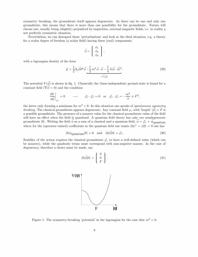
The potential V (~φ) is shown in fig. 1. Classically the (time-independent) ground state is found for a

constant field (∇~φ = 0) and the condition

∂V

∂~φ

∣∣∣∣ϕc

= 0 −→ ~ϕc · ~ϕc = 0 or ~ϕc · ~ϕc = −m2

λ≡ F 2,

the latter only forming a minimum for m2 < 0. In this situation one speaks of spontaneous symmetry

breaking. The classical groundstate appears degenerate. Any constant field ϕc with ’length’ |~φ| = F isa possible groundstate. The presence of a nonzero value for the classical groundstate value of the fieldwill have an effect when the field is quantized. A quantum field theory has only one nondegenerategroundstate |0〉. Writing the field ~φ as a sum of a classical and a quantum field, ~φ = ~ϕc + ~φquantumwhere for the (operator-valued) coefficients in the quantum field one wants 〈0|c† = c|0〉 = 0 one has

〈0|φquantum|0〉 = 0 and 〈0|~φ|0〉 = ~ϕc. (30)

Stability of the action requires the classical groundstate ~ϕc to have a well-defined value (which canbe nonzero), while the quadratic terms must correspond with non-negative masses. In the case ofdegeneracy, therefore a choice must be made, say

〈0|~φ|0〉 =

00F

. (31)

V( )φ

|φ|F

Figure 1: The symmetry-breaking ’potential’ in the lagrangian for the case that m2 < 0.

6

The situation now is the following. The original lagrangian contained an SO(3) invariance under(length conserving) rotations among the three fields, while the lagrangian including the nonzerogroundstate expectation value chosen by nature, has less symmetry. It is only invariant under ro-tations around the 3-axis.

It is appropriate to redefine the field as

~φ =

ϕ1

ϕ2

F + η

, (32)

such that 〈0|ϕ1|0〉 = 〈0|ϕ2|0〉 = 〈0|η|0〉 = 0. The field along the third axis plays a special role becauseof the choice of the vacuum expectation value. In order to see the consequences for the particlespectrum of the theory we construct the lagrangian in terms of the fields ϕ1, ϕ2 and η. It is sufficientto do this to second order in the fields as the higher (cubic, etc.) terms constitute interaction terms.The result is

L =1

2(∂µϕ1)

2 +1

2(∂µϕ2)

2 +1

2(∂µη)

2 − 1

2m2 (ϕ2

1 + ϕ22)

−1

2m2 (F + η)2 − 1

4λ (ϕ2

1 + ϕ22 + F 2 + η2 + 2Fη)2 (33)

=1

2(∂µϕ1)

2 +1

2(∂µϕ2)

2 +1

2(∂µη)

2 +m2 η2 + . . . . (34)

Therefore there are 2 massless scalar particles, corresponding to the number of broken generators (inthis case rotations around 1 and 2 axis) and 1 massive scalar particle with mass m2

η = −2m2. Themassless particles are called Goldstone bosons.

Realization of symmetries

In this section we want to discuss a bit more formal the two possible ways that a symmetry can beimplemented. They are known as the Weyl mode or the Goldstone mode:

Weyl mode. In this mode the lagrangian and the vacuum are both invariant under a set of symmetrytransformations generated by Qa, i.e. for the vacuum Qa|0〉 = 0. In this case the spectrum is describedby degenerate representations of the symmetry group. Known examples are rotational symmetry andthe fact that the the spectrum shows multiplets labeled by angular momentum ` (with memberslabeled by m). The generators Qa (in that case the rotation operators Lz, Lx and Ly or instead of thelatter two L+ and L−) are used to label the multiplet members or transform them into one another.A bit more formal, if the generators Qa generate a symmetry, i.e. [Qa, H ] = 0, and |a〉 and |a′〉 belongto the same multiplet (there is a Qa such that |a′〉 = Qa|a〉) then H |a〉 = Ea|a〉 implies that H |a′〉 =Ea|a′〉, i.e. a and a′ are degenerate states.

Goldstone mode. In this mode the lagrangian is invariant but Qa|0〉 6= 0 for a number of generators.This means that they are operators that create states from the vacuum, denoted |πa(k)〉. As thegenerators for a symmetry are precisely the zero-components of a conserved current J a

µ(x) integratedover space, there must be a nonzero expectation value 〈0|Ja

µ(x)|πa(k)〉. Using translation invarianceand as kµ is the only four vector on which this matrix element could depend one may write

〈0|Jaµ(x)|πb(k)〉 = fπ kµ e

i k·x δab (fπ 6= 0) (35)

for all the states labeled by a corresponding to ’broken’ generators. Taking the derivative,

〈0|∂µJaµ(x)|πb(k)〉 = fπ k

2 ei k·x δab = fπ m2πa ei k·x δab. (36)

7

If the transformations in the lagrangian give rise to a symmetry the Noether currents are conserved,∂µJa

µ = 0, irrespective of the fact if they annihilate the vacuum, and one must have mπa = 0, i.e. amassless Goldstone boson for each ’broken’ generator. Note that for the fields πa(x) one would havethe relation 〈0|πa(x)|πa(k)〉 = ei k·x, suggesting the stronger relation ∂µJa

µ(x) = fπ m2πa πa(x).

Chiral symmetry

An example of spontaneous symmetry breaking is chiral symmetry breaking in QCD. Neglecting atthis point the local color symmetry, the lagrangian for the quarks consists of the free Dirac lagrangianfor each of the types of quarks, called flavors. Including a sum over the different flavors (up, down,strange, etc.) one can write

L = ψ(i/∂ −M)ψ, (37)

where ψ is extended to a vector in flavor space and M is a diagonal matrix,

ψ =

ψu

ψd

...

, M =

mu

md

. . .

(38)

(Note that each of the entries in the vector for ψ is a 4-component Dirac spinor). This lagrangiandensity then is invariant under unitary (vector) transformations in the flavor space,

ψ −→ ei ~α·~Tψ, (39)

which for instance including only two flavors form an SU(2)V symmetry (isospin symmetry) gen-

erated by the Pauli matrices, ~T = ~τ/2. The conserved currents corresponding to this symmetrytransformation are found directly using Noether’s theorem (see chapter 6),

~V µ = ψγµ ~Tψ. (40)

Using the Dirac equation, it is easy to see that one gets

∂µ~V µ = i ψ [M, ~T ]ψ. (41)

Furthermore ∂µ~V µ = 0 ⇐⇒ [M, ~T ] = 0. From group theory (Schur’s theorem) one knows that the

latter can only be true, if in flavor space M is proportional to the unit matrix, M = m ·1. I.e. SU(2)V

(isospin) symmetry is good if the up and down quark masses are identical. This situation, both arevery small, is what happens in the real world. This symmetry is realized in the Weyl mode withthe spectrum of QCD showing an almost perfect isospin symmetry, e.g. a doublet (isospin 1/2) ofnucleons, proton and neutron, with almost degenerate masses (Mp = 938.3 MeV/c2 and Mn =939.6MeV/c2), but also a triplet (isospin 1) of pions, etc.

There exists another set of symmetry transformations, socalled axial vector transformations,

ψ −→ ei ~α·~Tγ5ψ, (42)

which for instance including only two flavors form SU(2)A transformations generated by the Pauli

matrices, ~Tγ5 = ~τγ5/2. Note that these transformations also work on the spinor indices. The currentscorresponding to this symmetry transformation are again found using Noether’s theorem,

~Aµ = ψγµ ~Tγ5ψ. (43)

Using the Dirac equation, it is easy to see that one gets

∂µ~Aµ = i ψ M, ~T γ5 ψ. (44)

8

In this case ∂µ~Aµ = 0 will be true if the quarks have zero mass, which is approximately true for the up

and down quarks. Therefore the world of up and down quarks describing pions, nucleons and atomicnuclei has not only an isospin or vector symmetry SU(2)V but also an axial vector symmetry SU(2)A.This combined symmetry is what one calls chiral symmetry.

That the massless theory has this symmetry can also be seen by writing it down for the socalledlefthanded and righthanded fermions, ψR/L = 1

2 (1 ± γ5)ψ, in terms of which the Dirac lagrangiandensity looks like

L = i ψL/∂ψL + i ψR/∂ψR − ψRMψL − ψLMψR. (45)

If the mass is zero the lagrangian is split into two disjunct parts for L and R showing that there isa direct product SU(2)L ⊗ SU(2)R symmetry, generated by ~TR/L = 1

2 (1 ± γ5)~T , which is equivalentto the V-A symmetry. This symmetry, however, is by nature not realized in the Weyl mode. Howcan we see this. The chiral fields ψR and ψL are transformed into each other under parity. Thereforerealization in the Weyl mode would require that all particles come double with positive and negativeparity, or, stated equivalently, parity would not play a role in the world. We know that mesons andbaryons (such as the nucleons) have a well-defined parity that is conserved.

The conclusion is that the original symmetry of the lagrangian is spontaneously broken and as thevector part of the symmetry is the well-known isospin symmetry, nature has choosen the path

SU(2)L ⊗ SU(2)R =⇒ SU(2)V ,

i.e. the lagrangian density is invariant under left (L) and right (R) rotations independently, while thegroundstate is only invariant under isospin rotations (R = L). From the number of broken generatorsit is clear that one expects three massless Goldstone bosons, for which the field (according to thediscussion above) has the same behavior under parity, etc. as the quantity ∂µA

µ(x), i.e. (leavingout the flavor structure) the same as ψγ5ψ, i.e. behaves as a pseudoscalar particle (spin zero, parityminus). In the real world, where the quark masses are not completely zero, chiral symmetry is notperfect. Still the basic fact that the generators acting on the vacuum give a nonzero result (i.e. fπ 6= 0remains, but the fact that the symmetry is not perfect and the right hand side of Eq. 44 is nonzero,gives also rise to a nonzero mass for the Goldstone bosons according to Eq. 36. The Goldstone bosonsof QCD are the pions for which fπ = 93 MeV and which have a mass of mπ ≈ 138 MeV/c2, muchsmaller than any of the other mesons or baryons.

3 The Higgs mechanism

The Higgs mechanism occurs when spontaneous symmetry breaking happens in a gauge theory wheregauge bosons have been introduced in order to assure the local symmetry. Considering the sameexample with rotational symmetry (SO(3)) as for spontaneous symmetry breaking of a scalar field(Higgs field) with three components, made into a gauge theory,

L = −1

4~Gµν · ~Gµν +

1

2Dµ

~φ ·Dµ~φ− V (~φ), (46)

whereDµ

~φ = ∂µ~φ− igW a

µLa~φ. (47)

Since the explicit (conjugate, in this case three-dimensional) representation (La)ij = −i εaij one sees

that the fields ~Wµ and ~Gµν also can be represented as three-component fields,

Dµ~φ = ∂µ

~φ+ g ~Wµ × ~φ, (48)

~Gµν = ∂µ~Wν − ∂ν

~Wµ + g ~Wµ × ~Wν . (49)

9

The symmetry is broken in the same way as before and the same choice for the vacuum,

~ϕc = 〈0|~φ|0〉 =

00F

.

is made. The difference comes when we reparametrize the field ~φ. We have the possibility to performlocal gauge transformations. Therefore we can always rotate the field φ into the z-direction in orderto make the calculation simple, i.e.

~φ =

00φ3

=

00

F + η

. (50)

Explicitly one then has

Dµ~φ = ∂µ

~φ+ g ~Wµ × ~φ =

gF W 2µ + gW 2

µ η−gF W 1

µ − gW 1µ η

∂µη

,

which gives for the lagrangian density up to quadratic terms

L = −1

4~Gµν · ~Gµν +

1

2Dµ

~φ ·Dµ~φ− 1

2m2~φ · ~φ− λ

4(~φ · ~φ)2

= −1

4(∂µ

~Wν − ∂ν~Wµ) · (∂µ ~W ν − ∂ν ~W µ) − 1

2g2F 2

(W 1

µWµ 1 +W 2

µWµ 2)

+1

2(∂µη)

2 +m2 η2 + . . . , (51)

from which one reads off that the particle content of the theory consists of one massless gauge boson(W 3

µ), two massive bosons (W 1µ and W 2

µ with MW = gF ) and a massive scalar particle (η with m2η =

−2m2. The latter is a spin 0 particle (real scalar field) called a Higgs particle. Note that the numberof massless gauge bosons (in this case one) coincides with the number of generators corresponding tothe remaining symmetry (in this case rotations around the 3-axis), while the number of massive gaugebosons coincides with the number of ’broken’ generators.

One may wonder about the degrees of freedom, as in this case there are no massless Goldstonebosons. Initially there are 3 massless gauge fields (each, like a photon, having two independent spincomponents) and three scalar fields (one degree of freedom each), thus 9 independent degrees offreedom. After symmetry breaking the same number (as expected) comes out, but one has 1 masslessgauge field (2), 2 massive vector fields or spin 1 bosons (2 × 3) and one scalar field (1), again 9 degreesof freedom.

4 The standard model SU(2)W ⊗ U(1)Y

The symmetry ideas discussed before play an essential role in the standard model that describesthe elementary particles, the quarks (up, down, etc.), the leptons (elektrons, muons, neutrinos, etc.)and the gauge bosons responsible for the strong, electromagnetic and weak forces. In the standardmodel one starts with a very simple basic lagrangian for (massless) fermions which exhibits moresymmetry than observed in nature. By introducing gauge fields and breaking the symmetry a morecomplex lagrangian is obtained, that gives a good description of the physical world. The procedure,however, implies certain nontrivial relations between masses and mixing angles that can be testedexperimentally and sofar are in excellent agreement with experiment.

The lagrangian for the leptons consists of three families each containing an elementary fermion(electron e−, muon µ− or tau τ−), its corresponding neutrino (νe, νµ and ντ ) and their antiparticles.

10

As they are massless, left- and righthanded particles, ψR/L = 12 (1 ± γ5)ψ decouple. For the neutrino

only a lefthanded particle (and righthanded antiparticle) exist. Thus

L (f) = i eR/∂eR + i eL/∂eL + i νeL/∂νeL + (µ, τ). (52)

One introduces a (weak) SU(2)W symmetry under which eR forms a singlet, while the lefthandedparticles form a doublet, i.e.

L =

νe

eL

with IW =1

2and I3

W =

+1/2−1/2

andR = eR with IW = 0 and I3

W = 0.

Thus the lagrangian density is

L (f) = i L/∂L+ i R/∂R, (53)

which has an SU(2)W symmetry under transformations ei~α·~T , explicitly

LSU(2)W−→ ei ~α·~τ/2L, (54)

RSU(2)W−→ R. (55)

One notes that the charges of the leptons can be obtained as Q = I3W − 1/2 for lefthanded particles

and Q = I3W − 1 for righthanded particles. This is written as

Q = I3W +

YW

2, (56)

and YW is considered as an operator that generates a U(1)Y symmetry, under which the lefthandedand righthanded particles with YW (L) = −1 and YW (R) = −2 transform with eiβYW /2, explicitly

LU(1)Y−→ e−i β/2L, (57)

RU(1)Y−→ e−i βR. (58)

Next the SU(2)W ⊗U(1)Y symmetry is made into a local symmetry introducing gauge fields ~Wµ andBµ,

DµL = ∂µL+i

2g ~Wµ · ~τ L− i

2g′Bµ L, (59)

DµR = ∂µR− i g′Bµ R, (60)

where ~Wµ is a triplet of gauge bosons with IW = 1, I3W = ±1 or 0 and YW = 0 (thus Q = I3

W ) andBµ is a singlet under SU(2)W (IW = I3

W = 0) and also has YW = 0. Putting this in leads to

L (f) = L (f1) + L (f2), (61)

L (f1) = i Rγµ(∂µ − ig′Bµ)R+ i Lγµ(∂µ − i

2g′Bµ +

i

2g ~Wµ · ~τ )L

L (f2) = −1

4(∂µ

~Wν − ∂ν~Wµ + g ~Wµ × ~Wν)2 − 1

4(∂µBν − ∂νBµ)2.

In order to break the symmetry to the symmetry of the physical world, the U(1)Q symmetry (generatedby the charge operator), a complex Higgs field

φ =

φ+

φ0

=

1√2(θ2 + iθ1)

1√2(θ4 − iθ3)

(62)

11

with IW = 1/2 and YW = 1 is introduced, with the following lagrangian density consisting of asymmetry breaking piece and a coupling to the fermions,

L (h) = L (h1) + L (h2), (63)

where

L (h1) = (Dµφ)†(Dµφ)−m2 φ†φ− λ (φ†φ)2︸ ︷︷ ︸

−V (φ)

,

L (h2) = −Ge(LφR +Rφ†L),

and

Dµφ = (∂µ +i

2g ~Wµ · ~τ +

i

2g′Bµ)φ. (64)

The Higgs potential V (φ) is choosen such that it gives rise to spontaneous symmetry breaking withϕ†

cϕ = −m2/2λ ≡ v2/2. For the classical field the choice θ4 = v is made. Using local gauge invariance

θi for i = 1, 2 and 3 may be eliminated (the necessary SU(2)W rotation is precisely e−i~θ(x)·τ ), leadingto the parametrization

φ(x) =1√2

0

v + h(x)

(65)

and

Dµφ =

ig2

(W 1

µ−iW 2µ√

2

)

(v + h)

∂µh− i2

(gW 3

µ−g′Bµ√2

)

(v + h)

. (66)

Up to cubic terms, this leads to the lagrangian

L (h1) =1

2(∂µh)

2 +m2 h2 +g2 v2

8

[(W 1

µ )2 + (W 2µ)2]

+v2

8

(gW 3

µ − g′Bµ

)2+ . . . (67)

=1

2(∂µh)

2 +m2 h2 +g2 v2

8

[(W+

µ )2 + (W−µ )2

]

+(g2 + g′2) v2

8(Zµ)2 + . . . , (68)

where the quadratically appearing gauge fields that are furthermore eigenstates of the charge operatorare

W±µ =

1√2

(W 1

µ ± iW 2µ

), (69)

Zµ =gW 3

µ − g′Bµ√

g2 + g′2≡ cos θW W 3

µ − sin θW Bµ, (70)

Aµ =g′W 3

µ + g Bµ√

g2 + g′2≡ sin θW W 3

µ + cos θW Bµ, (71)

and correspond to three massive particle fields (W± and Z0) and one massless field (photon γ) with

M2W =

g2 v2

4, (72)

M2Z =

g2 v2

4 cos2 θW=

M2W

cos2 θW, (73)

M2γ = 0. (74)

12

The weak mixing angle is related to the ratio of coupling constants, g′/g = tan θW .The coupling of the fermions to the physical gauge bosons are contained in L (f1) giving

L (f1) = i eγµ∂µe+ i νeγµ∂µνe − g sin θW eγµeAµ

+g

cos θW

(

sin2 θW eRγµeR − 1

2cos 2θW eLγ

µeL +1

2νeγ

µνe

)

Zµ

+g√2

(νeγ

µeLW−µ + eLγ

µνeW+µ

). (75)

From the coupling to the photon, we can read off

e = g sin θW = g′ cos θW . (76)

The coupling of electrons or muons to their respective neutrinos, for instance in the amplitude forthe decay of the muon

µν µν

µ−µ−e− e−

νe

νe

−W =

is given by

−iM = −g2

2(νµγ

ρµL)−i gρσ + . . .

k2 +M2W

(eLγσνe)

≈ ig2

8M2W

(νµγρ(1 − γ5)µ)

︸ ︷︷ ︸

(j(µ)†

L)ρ

(eγσ(1 − γ5)νe)︸ ︷︷ ︸

(j(e)

L)ρ

(77)

≡ iGF√

2(j

(µ)†L )ρ (j

(e)L )ρ, (78)

the good old four-point interaction introduced by Fermi to explain the weak interactions, i.e. one hasthe relation

GF√2

=g2

8M2W

=e2

8M2W sin2 θW

=1

2 v2. (79)

In this way the parameters g, g′ and v determine a number of experimentally measurable quantities,such as

e2/4π ≈ 1/137, (80)

GF = 1.166 4× 10−5 GeV−2, (81)

sin2 θW = 0.231 1, (82)

MW = 80.42 GeV, (83)

MZ = 91.198 GeV. (84)

The coupling of the Z0 to fermions is given by g/ cos θW multiplied with

I3W

1

2(1 − γ5) − sin2 θW Q ≡ 1

2CV − 1

2CA γ5, (85)

13

with

CV = I3W − 2 sin2 θW Q, (86)

CA = I3W . (87)

From this coupling it is straightforward to calculate the partial width for Z0 into a fermion-antifermionpair,

Γ(Z0 → ff) =MZ

48π

g2

cos2 θW(C2

V + C2A). (88)

For the electron, muon or tau, leptons with CV = −1/2 + 2 sin2 θW ≈ −0.05 and CA = −1/2 wecalculate Γ(e+e−) ≈ 78.5 MeV (exp. Γe ≈ Γµ ≈ Γτ ≈ 83 MeV). For each neutrino species (with CV =1/2 and CA = 1/2 one expects Γ(νν) ≈ 155 MeV. Comparing this with the total width into (invisible!)channels, Γinvisible = 480 MeV one sees that three families of (light) neutrinos are allowed. Actuallyincluding corrections corresponding to higher order diagrams the agreement for the decay width intoelectrons can be calculated much more accurately and the number of allowed (light) neutrinos turnsto be even closer to three.

The masses of the fermions and the coupling to the Higgs particle are contained in L (h2). Withthe choosen vacuum expectation value for the Higgs field, one obtains

L (h2) = −Ge v√2

(eLeR + eReL) − Ge√2

(eLeR + eReL)h

= −me ee−me

veeh. (89)

First, the mass of the electron comes from the spontaneous symmetry breaking but is not predicted(it is in the coupling Ge). The coupling to the Higgs particle is weak as the value for v calculated e.g.from the MW mass is about 250 GeV, i.e. me/v is extremely small.

Finally we want to say something about the weak properties of the quarks, as appear for instancein the decay of the neutron or the decay of the Λ (quark content uds),

e-

νe

-W

d

u

n −→ pe−νe ⇐⇒ d −→ ue−νe,

e-

νe

-W

u

s

Λ −→ pe−νe ⇐⇒ s −→ ue−νe.

The quarks also turn out to fit into doublets of SU(2)W for the lefthanded species and into singletsfor the righthanded quarks. A complication arises as it are not the ’mass’ eigenstates that appear inthe weak isospin doublets but linear combinations of them,

ud′

L

cs′

L

tb′

L

,

where

d′

s′

b′

L

=

Vud Vus Vub

Vcd Vcs Vcb

Vtd Vts Vtb

dsb

L

(90)

This mixing allows all quarks with I3W = −1/2 to decay into an up quark, but with different strength.

Comparing neutron decay and Λ decay one can get an estimate of the mixing parameter Vus in thesocalled Cabibbo-Kobayashi-Maskawa mixing matrix. Decay of B-mesons containing b-quarks allow

14

estimate of Vub, etc. In principle one complex phase is allowed in the most general form of the CKMmatrix, which can account for the (observed) CP violation of the weak interactions. This is onlytrue if the mixing matrix is at least three-dimensional, i.e. CP violation requires three generations.The magnitudes of the entries in the CKM matrix are nicely represented in a socalled Wolfensteinparametrization

V =

1 − 12 λ

2 λ λ3A(ρ− i η)−λ 1 − 1

2 λ2 λ2A

λ3A(1 − ρ− i η) −λ2A 1

+ O(λ4)

with λ ≈ 0.23, A ≈ 0.81 and ρ ≈ 0.23 and η ≈ 0.35. The imaginary part i η gives rise to CP violationin decays of K and B-mesons (containing s and b quarks, respectively).

5 Family mixing in the Higgs sector and neutrino masses

The quark sector

Allowing for the most general (Dirac) mass generating term in the lagrangian one starts with

L (h2,q) = −QLφΛdDR −DRΛ†dφ

†QL,−QLφcΛuUR − URΛ†

uφc†QL (91)

where we include now the three lefthanded quark doublets in QL, the three righthanded quarks withcharge +2/3 in UR and the three righthanded quarks with charges −1/3 inDR, each of these containingthe three families, e.g. UR =

(uR cR tR

). The Λu and Λd are complex matrices in the 3× 3 family

space. The Higgs field is still limited to one complex doublet. Note that we need the conjugate Higgsfield to get a U(1)Y singlet in the case of the charge +2/3 quarks, for which we need the appropriateweak isospin doublet

φc =

(φ0∗

−φ−)

=1√2

(v + h

0

)

.

For the (squared) complex matrices we can find positive eigenvalues,

Λu Λ†u = Vu G

2u V

†u , and Λd Λ†

d = WdG2dW

†d , (92)

where Vu and Wd are unitary matrices, allowing us to write

Λu = VuGu W†u and Λd = VdGdW

†d , (93)

with Gu and Gd being real and positive and Wu and Vd being different unitary matrices. Thus onehas

L (h2,q) =⇒ −DLVdMdW†dDR −DRWdMd V

†dDL,−ULVuMuW

†uUR − URWu Mu V

†uUL (94)

with Mu = Guv/√

2 (diagonal matrix containingmu, mc andmt) and Md = Gdv/√

2 (diagonal matrixcontaining md, ms and mb). One then reads off that starting with the family basis as defined via theleft doublets that the mass eigenstates (and states coupling to the Higgs field) involve the righthanded

states UmassR = W †

uUR and DmassR = W †

dDR and the lefthanded states UmassL = V †

uUL and DmassL =

V †dDL. Working with the mass eigenstates one simply sees that the weak current coupling to the W±

becomes UL γµγ5DL, U

mass

L γµγ5 V†uVdD

massL , i.e. the weak mass eigenstates are

D′L = Dweak

L = V †u VdD

massL = VCKMDmass

L , (95)

the unitary CKM-matrix introduced above in an ad hoc way.

15

The lepton sector (massless neutrinos)

For a lepton sector with a lagrangian density of the form

L (h2,`) = −LφΛeER −ERΛ†eφ

†L, (96)

in which

L =

(NL

EL

)

,

is a weak doublet containing the three families of neutrinos (NL) and charged leptons (EL) and ER isa three-family weak singlet, we find massless neutrinos. As before, one can write Λe = Ve GeW

†e and

we find

L (h2,`) =⇒ −Me

(ELVeW

†eER −ERWeV

†e EL

), (97)

with Me = Gev/√

2 the diagonal mass matrix with masses me, mµ and mτ . The mass fields EmassR

= W †eER, Emass

L = V †e EL and the neutrino fields Nmass

L = V †e NL are also the states appearing in the

W -current, i.e. there is no family mixing and the neutrinos are massless.

The lepton sector (massive Dirac neutrinos)

In principle a massive Dirac neutrino could be accounted for by a lagrangian of the type

L (h2,`) = −LφΛeER −ERΛ†eφ

†L,−LφcΛnNR −NRΛ†nφ

c†L (98)

with three righthanded neutrinos added to the previous case, decoupling from all known interactions.Again we continue as before now with matrices Λe = VeGe W

†e and Λn = Vn GnW

†n, and obtain

L (h2,`) =⇒ −ELVe MeW†eER −ERWe Me V

†e EL,−NLVnMnW

†nNR −NRWn Mn V

†nNL. (99)

We note that there are mass fields EmassR = W †

eER, EmassL = V †

e EL, NmassL = V †

nNL and NmassR =

W †nNR and the weak current becomes EL γ

µγ5NL = EmassL γµγ5 V

†e VnN

massL . Working with the mass

eigenstates for the charged leptons we see that the weak eigenstates for the neutrinos are NweakL =

V †e NL with the relation to the mass eigenstates for the lefthanded neutrinos given by

N ′L = Nweak

L = V †e Vn N

massL , (100)

or NmassL = U Nweak

L with U = V †n Ve.

The lepton sector (massive Majorana fields)

The simplest option is to add in Eq. 97 a Majorana mass term for (lefthanded) neutrino mass eigen-states,

L mass,ν = −1

2

(MLN c

LNL +M∗LNLN

cL

), (101)

but this option is not attractive as it violates the electroweak symmetry. The way to circumvent thisis to introduce as in the previous section righthanded neutrinos with for the righthanded sector a massterm MR,

L mass,ν = −1

2

(MRNRN

cR +M∗

RNcRNR

). (102)

For neutrinos as well as charged leptons, the right- and lefthanded species are coupled through Diracmass terms as in the previous section. Thus (disregarding family structure) one has two Majorananeutrinos, one being massive. For the charged leptons there are no Majorana mass terms (it wouldbreak the U(1) electromagnetic symmetry) and left- and righthanded species combine to a Diracfermion. Moreover, if the Majorana mass MR MD one obtains in a natural way tiny neutrinomasses. This is called the seesaw mechanism.

16

The seesaw mechanism

Consider (for one family N = n) the most general Lorentz invariant mass term for two independentMajorana spinors, Υ′

1 and Υ′2 (satisfying Υc = Υ and as discussed in chapter 6, Υc

L ≡ (ΥL)c = ΥR

and ΥcR = ΥL). We use here the primes starting with the weak eigenstates. Actually, it is easy to see

that this incorporates the Dirac case by considering the lefthanded part of Υ′1 and the righthanded

part of Υ′2 as a Dirac spinor ψ. Thus

Υ′1 = nc

L + nL, Υ′2 = nR + nc

R, ψ = nR + nL. (103)

As the most general mass term in the lagrangian density we have

L mass = −1

2

(ML nc

L nL +M∗L nL n

cL

)− 1

2

(MR nR n

cR +M∗

R ncR nR

)

− 1

2

(MD nc

L ncR +M∗

D nL nR

)− 1

2

(MD nR nL +M∗

D ncR n

cL

)(104)

= −1

2

(nc

L nR)(

ML MD

MD MR

)(nL

ncR

)

+ h.c. (105)

which for MD = 0 is a pure Majorana lagrangian and for ML = MR = 0 and real MD represents theDirac case. The mass matrix can be written as

M =

(ML |MD| eiφ

|MD| eiφ MR

)

(106)

taking ML and MR real and non-negative. This choice is possible without loss of generality becausethe phases can be absorbed into Υ′

1 and Υ′2 (real must be replaced by hermitean if one includes

families). This is a mixing problem with a symmetric (complex) mass matrix leading to two (real)mass eigenstates. The diagonalization is analogous to what was done for the Λ-matrices and one findsU M UT = M0 with a (unitary) matrix U , which implies U∗M † U † = U∗M∗U † = M0 and a ’normal’diagonalization of the (hermitean) matrix MM †,

U (MM †)U † = M20 , (107)

Thus one obtains from

MM † =

(M2

L + |MD|2 |MD|(ML e

−iφ +MR e+iφ)

|MD|(ML e

+iφ +MR e−iφ)

M2R + |MD|2

)

, (108)

the eigenvalues

M21/2 =

1

2

[

M2L +M2

R + 2|MD|2

±√

(M2L −M2

R)2 + 4|MD|2 (M2L +M2

R + 2MLMR cos(2φ))

]

, (109)

and we are left with two decoupled Majorana fields Υ1 and Υ2, related via(

Υ1L

Υ2L

)

= U∗(nL

ncR

)

,

(Υ1R

Υ2R

)

= U

(nc

L

nR

)

. (110)

for each of which one finds the lagrangians

L =1

4Υi i

↔/∂ Υi −

1

2Mi Υi Υi (111)

for i = 1, 2 with real masses Mi. For the situation ML = 0 and MR MD (taking MD real) onefinds M1 ≈M2

D/MR and M2 ≈MR.

17

Exercises

Exercise 1

Consider the case of the Weyl mode for symmetries. Prove that if the generators Qa generate asymmetry, i.e. [Qa, H ] = 0, and |a〉 and |a′〉 belong to the same multiplet (there is a Qa such that|a′〉 = Qa|a〉) then H |a〉 = Ea|a〉 implies that H |a′〉 = Ea|a′〉, i.e. a and a′ are degenerate states.

Exercise 2

Derive for the vector and axial vector currents, ~V µ = ψγµ ~Tψ and ~Aµ = ψγµγ5~Tψ

∂µ~V µ = i ψ [M, ~T ]ψ,

∂µ~Aµ = i ψ M, ~T γ5 ψ.

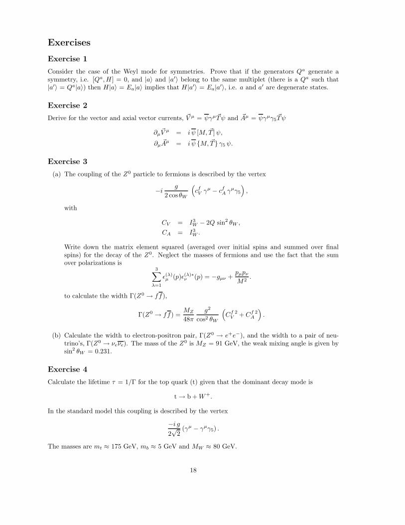
Exercise 3

(a) The coupling of the Z0 particle to fermions is described by the vertex

−i g

2 cos θW

(

cfV γµ − cfA γ

µγ5

)

,

with

CV = I3W − 2Q sin2 θW ,

CA = I3W .

Write down the matrix element squared (averaged over initial spins and summed over finalspins) for the decay of the Z0. Neglect the masses of fermions and use the fact that the sumover polarizations is

3∑

λ=1

ε(λ)µ (p)ε(λ)∗

ν (p) = −gµν +pµpν

M2.

to calculate the width Γ(Z0 → ff),

Γ(Z0 → ff) =MZ

48π

g2

cos2 θW

(

Cf 2V + Cf 2

A

)

.

(b) Calculate the width to electron-positron pair, Γ(Z0 → e+e−), and the width to a pair of neu-trino’s, Γ(Z0 → νeνe). The mass of the Z0 is MZ = 91 GeV, the weak mixing angle is given bysin2 θW = 0.231.

Exercise 4

Calculate the lifetime τ = 1/Γ for the top quark (t) given that the dominant decay mode is

t → b +W+.

In the standard model this coupling is described by the vertex

−i g2√

2(γµ − γµγ5) .

The masses are mt ≈ 175 GeV, mb ≈ 5 GeV and MW ≈ 80 GeV.

18

Exercise 5

Show that the coupling to the Higgs (W+W−h, ZZh, hhh and e+e−h) are proportional to the masssquared (bosons) or mass (fermions) of the particles. Note that you can find the answer withoutexplicit construction of the interaction terms lagrangian.

Exercise 6

Check that the Wolfenstein parametrization of the CKM matrix respects unitarity up to the required(which?) order in λ.

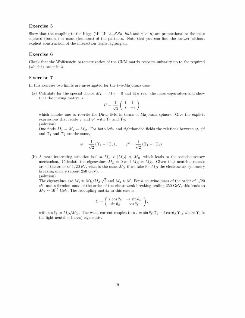
Exercise 7

In this exercise two limits are investigated for the two-Majorana case.

(a) Calculate for the special choice ML = MR = 0 and MD real, the mass eigenvalues and showthat the mixing matrix is

U =1√2

(1 1i −i

)

which enables one to rewrite the Dirac field in terms of Majorana spinors. Give the explicitexpressions that relate ψ and ψc with Υ1 and Υ2.(solution)One finds M1 = M2 = MD. For both left- and righthanded fields the relations between ψ, ψc

and Υ1 and Υ2 are the same,

ψ =1√2

(Υ1 + iΥ2) , ψc =1√2

(Υ1 − iΥ2) .

(b) A more interesting situation is 0 = ML < |MD| MR, which leads to the socalled seesawmechanism. Calculate the eigenvalues ML = 0 and MR = MX . Given that neutrino massesare of the order of 1/20 eV, what is the mass MX if we take for MD the electroweak symmetrybreaking scale v (about 250 GeV).(solution)The eigenvalues are M1 ≈ M2

D/MX

√2 and M2 ≈M . For a neutrino mass of the order of 1/20

eV, and a fermion mass of the order of the electroweak breaking scaling 250 GeV, this leads toMX ∼ 1015 GeV. The recoupling matrix in this case is

U =

(i cos θS −i sin θS

sin θS cos θS

)

,

with sin θS ≈ MD/MX . The weak current couples to nL = sin θS Υ2 − i cos θS Υ1, where Υ1 isthe light neutrino (mass) eigenstate.

19

A kinematics in scattering processes

Phase space

The 1-particle state is denoted |p〉. It is determined by the energy-momentum four vector p = (E,p)which satisfies p2 = E2−p2 =m2. A physical state has positive energy. The phase space is determinedby the weight factors assigned to each state in the summation or integration over states, i.e. the 1-particle phase space is

∫d3p

(2π)3 2E=

∫d4p

(2π)4θ(p0) (2π)δ(p2 −m2). (112)

This is generalized to the multi-particle phase space

dR(p1, . . . , pn) =

n∏

i=1

d3pi

(2π)3 2Ei, (113)

and the reduced phase space element by

dR(s, p1, . . . , pn) = (2π)4 δ4(P −∑

i

pi) dR(p1, . . . , pn), (114)

which is useful because the total 4-momentum of the final state usually is fixed by overall momentumconservation. Here s is the invariant mass of the n-particle system, s = (p1 + . . . + pn)2. It is auseful quantity, for instance for determining the threshold energy for the production of a final state1 + 2 + . . .+ n. In the CM frame the threshold value for s obviously is

sthreshold =

(n∑

i=1

mi

)2

. (115)

For two particle states |pa, pb〉 we start with the four vectors pa = (Ea,pa) and pb = (Eb,pb)satisfying p2

a = m2a and p2

b = m2b , and the total momentum four-vector P = pa +pb. For two particles,

the quantitys = P 2 = (pa + pb)

2, (116)

is referred to as the invariant mass squared. Its square root,√s is for obvious reasons known as the

center of mass (CM) energy.To be specific let us consider two frequently used frames. The first is the CM system. In that case

pa = (Ecma , q), (117)

pb = (Ecmb ,−q), (118)

It is straightforward to prove that the unknowns in the particular system can be expressed in theinvariants (ma, mb and s). Prove that

|q| =

√

(s−m2a −m2

b)2 − 4m2

am2b

4s=

√

λ(s,m2a,m

2b)

4s, (119)

Ecma =

s+m2a −m2

b

2√s

, (120)

Ecmb =

s−m2a +m2

b

2√s

. (121)

The function λ(s,m2a,m

2b) is a function symmetric in its three arguments, which in the specific case

also can be expressed as λ(s,m2a,m

2b) = 4(pa · pb)

2 − 4p2a p

2b .

20

The second frame considered explicitly is the socalled target rest frame in which one of the particles(called the target) is at rest. In that case

pa = (Etrfa ,ptrf

a ), (122)

pb = (mb,0), (123)

Also in this case one can express the energy and momentum in the invariants. Prove that

Etrfa =

s−m2a −m2

b

2mb, (124)

|ptrfa | =

√

λ(s,m2a,m

2b)

2mb. (125)

One can, for instance, use the first relation and the abovementioned threshold value for s to calculatethe threshold for a specific n-particle final state in the target rest frame,

Etrfa (threshold) =

1

2 mb

(

(∑

i

mi)2 − m2

a − m2b

)

. (126)

Explicit calculation of the reduced two-body phase space element gives

dR(s, p1, p2) =1

(2π)2d3p1

2E1

d3p2

2E2δ4(P − p1 − p2)

CM=

1

(2π)2d3q

4E1E2δ(√s−E1 −E2)

=1

(2π)2dΩ(q)

q2 d|q|4E1E2

δ(√s−E1 −E2)

which using |q| d|q| = E1 dE1 = E2 dE2 gives

dR(s, p1, p2) =|q|

(2π)2dΩ(q)

d(E1 +E2)

4(E1 +E2)δ(√s−E1 −E2)

=|q|

4π√s

dΩ(q)

4π=

√λ12

8π s

dΩ(q)

4π, (127)

where λ12 denotes λ(s,m21,m

22).

Kinematics of 2 → 2 scattering processes

The simplest scattering process is 2 particles in and 2 particles out. Examples appear in

π− + p → π− + p (128)

→ π0 + n (129)

→ π+ + π− + n (130)

→ . . . . (131)

The various possibilities are referred to as different reaction channels, where the first is referred toas elastic channel and the set of all other channels as the inelastic channels. Of course there are notonly 2-particle channels. The initial state, however, usually is a 2-particle state, while the final stateoften arises from a series of 2-particle processes combined with the decay of an intermediate particle(resonance).

21

Consider the process a+ b→ c+ d. An often used set of invariants are the Mandelstam variables,

s = (pa + pb)2 = (pc + pd)

2 (132)

t = (pa − pc)2 = (pb − pd)

2 (133)

u = (pa − pd)2 = (pb − pc)

2 (134)

which are not independent as s+ t+ u = m2a +m2

b +m2c +m2

d. The variable s is always larger thanthe minimal value (ma +mb)

2. A specific reaction channel starts contributing at the threshold value(Eq. 115). Instead of the scattering angle, which for the above 2 → 2 process in the case of azimuthalsymmetry is defined as pa · pc = cos θ one can use in the CM the invariant

t ≡ (pa − pc)2 CM

= m2a +m2

c − 2EaEc + 2 qq′ cos θcm,

with q =√λab/2

√s and q′ =

√λcd/2

√s. The minimum and maximum values for t correspond to θcm

being 0 or 180 degrees,

tmaxmin = m2

a +m2c − 2EaEc ± 2 qq′

= m2a +m2

c −(s+m2

a −m2b)(s+m2

c −m2d)

2 s±

√λλ′

2 s. (135)

Using the relation between t and cos θcm it is straightforward to express dΩcm in dt, dt = 2 qq′ d cos θcmand obtain for the two-body phase space element

dR(s, pc, pd) =q′

4π√s

dΩcm

4π=

√λcd

8π s

dΩcm

4π(136)

=dt

8π√λab

=dt

16π q√s. (137)

B Cross sections and lifetimes

Scattering process

For a scattering process a+ b → c+ . . . (consider for convenience the rest frame for the target, say b)the cross section σ(a+ b→ c+ . . .) is defined as the proportionality factor in

Nc

T= σ(a+ b→ c+ . . .) ·Nb · flux(a),

where V and T indicate the volume and the time in which the experiment is performed, Nc/T indicatesthe number of particles c detected in the scattering process, Nb indicates the number of (target)particles b, which for a density ρb is given by Nb = ρb · V , while the flux of the beam particles a isflux(a) = ρa ·vtrf

a . The proportionality factor has the dimension of area and is called the cross section,i.e.

σ =N

T · V1

ρaρb vtrfa

. (138)

Although this at first sight does not look covariant, it is. N and T · V are covariant. Using ρtrfa =

ρ(0)a · γa = ρ

(0)a ·Elab

a /ma (where ρ(0)a is the rest frame density) and vlab

a = plaba /Elab

a we have

ρaρb vtrfa =

ρ(0)a ρ

(0)b

4mamb2√

λab

or with ρ(0)a = 2ma,

σ =1

2√λab

N

T · V . (139)

22

Decay of particles

For the decay of particle a one has macroscopically

dN

dt= −ΓN, (140)

i.e. the amount of decaying particles is proportional to the number of particles with proportionalityfactor the em decay width Γ. From the solution

N(t) = N(0) e−Γ t (141)

one knows that the decay time τ = 1/Γ. Microscopically one has

Ndecay

T= Na · Γ

or

Γ =N

T · V1

ρa. (142)

This quantity is not covariant, as expected. The decay time for moving particles τ is related to thedecay time in the rest frame of that particle (the proper decay time τ0) by τ = γ τ0. For the (proper)decay width one thus has

Γ0 =1

2ma

N

T · V . (143)

Fermi’s Golden Rule

In both the scattering cross section and the decay constant the quantity N/TV appears. For this weemploy in essence Fermi’s Golden rule stating that when the S-matrix element is written as

Sfi = δfi − (2π)4 δ4(Pi − Pf ) iMfi (144)

(in which we can calculate −iMfi using Feynman diagrams), the number of scattered or decayedparticles is given by

N =∣∣(2π)4 δ4(Pi − Pf ) iMfi

∣∣2dR(p1, . . . , pn). (145)

One of the δ functions can be rewritten as T · V (remember the normalization of plane waves),

∣∣(2π)4 δ4(Pi − Pf )

∣∣2

= (2π)4 δ4(Pi − Pf )

∫

V,T

d4x ei(Pi−Pf )·x

= (2π)4 δ4(Pi − Pf )

∫

V,T

d4x = V · T (2π)4 δ4(Pi − Pf ).

(Using normalized wave packets these somewhat ill-defined manipulations can be made more rigorous).The result is

N

T · V = |Mfi|2 dR(s, p1, . . . , pn). (146)

Combining this with the expressions for the width or the cross section one obtains for the decay width

Γ =1

2m

∫

dR(m2, p1, . . . , pn) |M|2 (147)

2−body decay=

q

32π2m2

∫

dΩ |M |2. (148)

23

The differential cross section (final state not integrated over) is given by

dσ =1

2√λab

|Mfi|2 dR(s, p1, . . . , pn), (149)

and for instance for two particles

dσ =q′

q

∣∣∣∣

M(s, θcm)

8π√s

∣∣∣∣

2

dΩcm =π

λab

∣∣∣∣

M(s, t)

4π

∣∣∣∣

2

dt. (150)

This can be used to get the full expression for dσ/dt for eµ and e+e− scattering, for which theamplitudes squared have been calculated in the previous chapter. The amplitude −M/8π

√s is the

one to be compared with the quantum mechanical scattering amplitude f(E, θ), for which one hasdσ/dΩ = |f(E, θ)|2. The sign difference comes from the (conventional) sign in relation between S andquantummechanical and relativistic scattering amplitude, respectively.

C Unitarity condition

The unitarity of the S-matrix, i.e.(S†)fn Sni = δfi

implies for the scattering matrix M,

[δfn + i(2π)4 δ4(Pf − Pn) (M†)fn

] [δni − i(2π)4 δ4(Pi − Pn)Mni

]= δfi,

or−i[Mfi − (M†)fi

]= −

∑

n

(M†)fn (2π)4 δ4(Pi − Pn)Mni. (151)

Since the amplitudes also depend on all momenta the full result for two-particle intermediate statesis (in CM, see 136)

−i[Mfi − (M†)fi

]= −

∑

n

∫

dΩ(qn)M∗nf (qf , qn)

qn16π2

√sMni(qi, qn). (152)

Partial wave expansion

Often it is useful to make a partial wave expansion for the amplitude M(s, θ) or M(qi, qf ),

M(s, θ) = −8π√s∑

`

(2`+ 1)M`(s)P`(cos θ), (153)

(in analogy with the expansion for f(E, θ) in quantum mechanics; note the sign and cos θ = qi · qf ).Inserted in the unitarity condition for M,

i

[ M8π

√s− M†

8π√s

]

fi

=∑

n

∫

dΩn

M∗nf

8π√s

qn2π

Mni

8π√s,

we obtainLHS = −i

∑

`

(2`+ 1)P`(qi · qf )(

(M`)fi − (M †` )fi

)

,

while for the RHS use is made of

P`(q · q′) =∑

m

4π

2`+ 1Y (`)

m (q)Y (`)∗m (q′)

24

and the orthogonality of the Y(`)m functions to prove that

RHS = 2∑

n

∑

`

(2`+ 1)P`(qi · qf ) (M †` )fn qn (M`)ni,

i.e.−i(

(M`)fi − (M †` )fi

)

= 2∑

n

(M †` )fn qn (M`)ni. (154)

If only one channel is present this simplifies to

−i (M` −M∗` ) = 2 qM∗

` M`, (155)

or ImM` = q |M`|2, which allows writing

M`(s) =S`(s) − 1

2i q=e2i δ`(s) − 1

2i q, (156)

where S`(s) satisfies |S`(s)| = 1 and δ`(s) is the phase shift.In general a given channel has |S`(s)| ≤ 1, parametrized as S`(s) = η`(s) exp(2i δ`(s)). Using

σ =

∫

dΩq′

q

∣∣∣∣

M(s, θcm)

8π√s

∣∣∣∣

2

,

in combination with the partial wave expansion for the amplitudes M and the orthogonality of theLegendre polynomials immediately gives for the elastic channel,

σel = 4π∑

`

(2`+ 1)|M (`)(s)|2

=4π

q2

∑

`

(2`+ 1)

∣∣∣∣

η` e2i δ` − 1

2i

∣∣∣∣

2

, (157)

and for the case that this is the only channel (purely elastic scattering, η = 1) the result

σel =4π

q2

∑

`

(2`+ 1) sin2 δ`. (158)

From the imaginary part of M(s, 0), the total cross section can be determined. Show that

σT =4π

q

∑

`

(2`+ 1) ImM (`)(s)

=2π

q2

∑

`

(2`+ 1) (1 − η` cos 2δ`). (159)

The difference is the inelastic cross section,

σinel =π

q2

∑

`

(2`+ 1) (1 − η2` ). (160)

Note that the total cross section is maximal in the case of full absorption, η = 0, in which case,however, σel = σinel.

We note that unitarity is generally broken in a finite order calculation. Relating ImM and |M|2we obtain relations between terms at different order in the coupling constant.

25

D Unstable particles

For a stable particle the propagator is

i∆(k) =i

k2 −M2 + iε(161)

(note that we have disregarded spin). The prescription for the pole structure, i.e. one has poles at k0

= ±(E − iε) where E = +√

k2 +M2 guarantees the correct behavior, specifically one has for t > 0that the Fourier transform is

∫

dk0 e−ik0t ∆(k) ∝∫

dk0 e−ik0t

(k0 −E + iε)(k0 +E − iε)

(t>0)∝ e−iEt,

i.e. ∝ U(t, 0), the time-evolution operator. For an unstable particle one expects that

U(t, 0) ∝ e−i(E−iΓ/2)t,

such that |U(t, 0)|2 = e−Γt. This is achieved with a propagator

i∆R(k) =i

k2 −M2 + iMΓ(162)

(again disregarding spin). The quantity Γ is precisely the width for unstable particles. This is(somewhat sloppy!) seen by considering the (amputated) 1PI two-point vertex

Γ(2) =−i∆

as the amplitude −iM for scattering a particle into itself through the decay channels as intermediatestates. The unitarity condition then states

2 Im∆−1R (k) =

∑

n

∫

dR(p1, . . . , pn)M†Rn (2π)4 δ4(k − Pn)MnR

= 2M∑

n

Γn = 2M Γ. (163)

This shows that Γ is the width of the resonance, which is given by a sum of the partial widths intothe different channels. It is important to note that the physical width of a particle is the imaginarypart of the two-point vertex at s = M 2.

For the amplitude in a scattering process going through a resonance, it is straightforward to writedown the partial wave amplitude,

(qM`)ij(s) =−M

√ΓiΓj

s−M2 + iMΓ. (164)

(Prove this using the unitarity condition for partial waves). From this one sees that a resonance hasthe same shape in all channels but different strength. Limiting ourselves to a resonance in one channel,it is furthermore easy to prove that the cross section is given by

σel =4π

q2(2`+ 1)

M2Γ2

(s−M2)2 +M2Γ2, (165)

reaching the unitarity limit for s = M 2, where furthermore σinel = 0. This characteristic shape of aresonance is called the Breit-Wigner shape. The half-width of the resonance is MΓ. The phase shiftin the resonating channel near the resonance is given by

tan δ`(s) =MΓ

M2 − s, (166)

26

showing that the phase shift at resonance rises through δ = π/2 with a ’velocity’ ∂δ/∂s = 1/MΓ,i.e. a fast change in the phase shift for a narrow resonance. Note that because of the presence of abackground the phase shift at resonance may actually be shifted.Three famous resonances are:

• The ∆-resonance seen in pion-nucleon scattering. Its mass is M = 1232 MeV, its width Γ =120 MeV. At resonance the cross section σT (π+p) is about 210 mb. The cross section σT (π−p)also shows a resonance with the same width with a value of about 70 mb. This implies that theresonance has spin J = 3/2 (decaying in a P-wave (` = 1) pion-nucleon state) and isospin I =3/2 (the latter under the assumption that isospin is conserved for the strong interactions).

• The J/ψ resonance in e+e− scattering. This is a narrow resonance discovered in 1974. Its massis M = 3096.88 MeV, the full width is Γ = 88 keV, the partial width into e+e− is Γee = 5.26keV.

• The Z0 resonance in e+e− scattering with M = 91.2 GeV, Γ = 2.49 GeV. Essentially thisresonance can decay into quark-antiquark pairs or into pairs of charged leptons. All thesedecays can be seen and leave an ’invisible’ width of 498 MeV, which is attributed to neutrinos.Knowing that each neutrino contributes about 160 MeV, one can reconstruct the resonanceshape for different numbers of neutrino species. Three neutrinos explain the resonance shape.The cross section at resonance is about 30 nb.

27