THE SQUARE ROOTS OF SOME CLASSICAL OPERATORS

THE SQUARE ROOTS OF SOME CLASSICAL OPERATORS

JAVAD MASHREGHI, MAREK PTAK, AND WILLIAM T. ROSS

ABSTRACT. In this paper we give complete descriptions of the set ofsquare roots of certain classical operators, often providing specific for-mulas. The classical operators included in this discussion are the squareof the unilateral shift, the Volterra operator, certain compressed shifts, theunilateral shift plus its adjoint, the Hilbert matrix, and the Cesaro opera-tor.

1. INTRODUCTION

IfH is a complex Hilbert space andA ∈ B(H), the bounded linear operatorson H, when does A have a square root? By this we mean, does there exista B ∈ B(H) such that B2 = A? If A has a square root, can we describe{B ∈ B(H) : B2 = A}, the set of all the square roots of A?

First let us make the, perhaps unexpected, observation that not every op-erator has a square root. For example, Halmos showed that the unilateralshift Sf = zf on the Hardy space H2 [4] does not have a square root [6].Other examples of operators constructed with the shift S and its adjoint S∗,for example S ⊕ S∗ and S ⊗ S∗, also do not have square roots [2]. See thepapers [8, 12, 13, 18, 19] for some general results concerning square roots ofoperators.

Second, many operators have an abundance of square roots. For example,any nilpotent operator of order two is a square root of the zero operator.Moreover, to highlight their abundance, Lebow proved (see [7, Prob. 111])that when dimH =∞, the set {A ∈ B(H) : A2 = 0} is dense in B(H) in thestrong operator topology.

Much of the work on square roots has focused on the general topic of whichoperators have square roots and the prevalence of types of square roots (pthroots and logarithms) in B(H). Previous papers also have results which ex-plore the relationship between the type of square root as related to the typeof operator. In this paper, we focus on a collection of some well-knownclassical operators and proceed to characterize all of their square roots. The

2010 Mathematics Subject Classification. 47B35, 47B02, 47A05.Key words and phrases. Hardy spaces, Toeplitz operators, shift operator, compressed

shift, Volterra operator, Cesaro operator, Hilbert matrix.This work was supported by the NSERC Discovery Grant (Canada) and by the Ministry

of Science and Higher Education of the Republic of Poland.1

arX

iv:2

109.

1368

8v1

[m

ath.

FA]

28

Sep

2021

2 J. MASHREGHI, M. PTAK, AND W. ROSS

classical operators included in this discussion are the square of the unilat-eral shift (Theorem 2.4), the Volterra operator (Theorem 3.7), certain com-pressed shifts (Theorem 4.1), the unilateral shift plus its adjoint (Theorem5.2), the Hilbert matrix (Theorem 6.2), and the Cesaro operator (Theorem7.2 and Theorem 7.4). Our work on the Cesaro operator answers a questionposed in [12] and stems from a question posed by Halmos.

2. SQUARE ROOTS OF S2

Suppose that (Sf)(z) = zf(z) denotes the unilateral shift on the Hardyspace H2 [11]. In this section we explore the square roots of S2. One squareroot of S2 is, of course, S itself. Our characterization of all of the squareroots of S2, requires a few preliminaries.

For g ∈ H2, let

ge(z) := 12(g(z) + g(−z)) and go(z) := 1

2(g(z)− g(−z))

and observe that g(z) = ge(z) + go(z). If g(z) =∑∞

n=0 anzn, then

ge(z) =∞∑k=0

a2kz2k and go(z) =

∞∑k=0

a2k+1z2k+1.

This is the “even” and “odd” decomposition of g since ge(−z) = ge(z) andgo(−z) = −go(z). Finally, let

(Wg)(z) =

∞∑k=0

a2kzk

∞∑k=0

a2k+1zk

and note that W is a unitary operator from H2 onto

H2 ⊕H2 ={[

fg

]: f, g ∈ H2

},

with

W ∗[g1

g2

]= g1(z2) + zg2(z2).

Our last bit of notation is the vector-valued shift

S ⊕ S : H2 ⊕H2 → H2 ⊕H2, (S ⊕ S)

[g1

g2

]=

[Sg1

Sg2

].

It is traditional to think of S ⊕ S in matrix form as

S ⊕ S =

[S 00 S

].

The above formulas yield the following well-known fact.

SQUARE ROOT 3

Proposition 2.1. W ∗(S ⊕ S)W = S2.

Some other well-known facts used in the section involve the commutantsof S and S ⊕ S. For ϕ ∈ H∞, the bounded analytic functions on D, theToeplitz (Laurent) operator Tϕg = ϕg is bounded on H2 and STϕ = TϕS.Let

{S}′ = {A ∈ B(H2) : SA = AS}denote the commutant of S. The following fact is standard [20, Thm. 3.4].

Proposition 2.2. {S}′ = {Tϕ : ϕ ∈ H∞}.

In a similar way, let

Φ =

[Φ11 Φ12

Φ21 Φ22

],

where Φij ∈ H∞. We use the notationM2(H∞) for the 2×2 matrices abovewith H∞ entries. Define TΦ : H2 ⊕H2 → H2 ⊕H2 by

TΦ

[g1

g2

]=

[Φ11 Φ12

Φ21 Φ22

] [g1

g2

]=

[Φ11g1 + Φ12g2

Φ21g1 + Φ22g2

].

A calculation shows that (S ⊕ S)TΦ = TΦ(S ⊕ S). Similar to the above, wehave the following [20, Cor. 3.20].

Proposition 2.3. {S ⊕ S}′ = {TΦ : Φ ∈M2(H∞)}.

Here is the main theorem of this section describing all of the square rootsof S2.

Theorem 2.4. For Q ∈ B(H2) the following are equivalent.

(i) Q2 = S2.

(ii) There is a 2× 2 constant unitary matrix U and functions a, b, c ∈ H∞ satis-fying

(2.5) za2 + bc = 1

such that

(2.6) Q = W ∗U∗[za bzc −za

]UW.

Proposition 2.1 shows that to prove Theorem 2.4, it suffices to prove thefollowing.

Theorem 2.7. For A ∈ B(H2 ⊕H2) the following are equivalent.

(i) A2 = S ⊕ S.


(ii) There is a 2× 2 constant unitary matrix U and functions a, b, c ∈ H∞ satis-fying

(2.8) za2 + bc = 1

such that

(2.9) A = U∗[za bzc −za

]U.

A matrix calculation shows that

A2 = U∗[za bzc −za

]UU∗

[za bzc −za

]U

= U∗[z2a2 + zbc 0

0 z2a2 + zbc

]U

= U∗[z 00 z

]U

= U∗(S ⊕ S)U

= S ⊕ S.In the above, we use the fact that any constant matrix commutes with S⊕S.Thus every operator of the form (2.9) is a square root of S ⊕ S. The rest ofthis section will be devoted to proving the converse – and providing someinstances of this characterization.

Our proof involves a few more preliminaries. The first is a simple fact aboutsquare roots of bounded Hilbert space operators.

Lemma 2.10. If B ∈ B(H) and A2 = B, then A ∈ {B}′.

Proof. Note that AB = AA2 = A2A = BA. �

Combining this with the discussion above, we see that if Q ∈ B(H2) withQ2 = S2, then WQW ∗ ∈ B(H2 ⊕H2) with (WQW ∗)2 = S ⊕ S. It followsfrom Lemma 2.10 and Proposition 2.3 that

WQW ∗ = A, A ∈M2(H∞).

To identify A, let us start with lemmas about 2× 2 matrices M2(C) of com-plex numbers. For X,Y ∈M2(C) let

[X,Y ]+ := XY + Y X.

One can quickly verify the following useful facts about the subspace

(2.11) S ={[

α βγ −α

]: α, β, γ ∈ C

}.

Lemma 2.12. Let α, β, γ, λ ∈ C.

SQUARE ROOT 5

(i) If

X =

[α β0 γ

]and X2 = 0, then α = γ = 0, in other words, X2 = 0 if and only if

X =

[0 β0 0

].

(ii) If

X =

[0 β0 0

]and Y ∈M2(C) with [X,Y ]+ = λI2 with λ 6= 0, then β 6= 0 and

Y =

[α ηλ/β −α

],

where α, η ∈ C are arbitrary.

(iii) If X,Y ∈ S, then X2 and [X,Y ]+ ∈ CI2.

For a sequence (Ak)∞k=0, where Ak ∈ M2(C) for all k > 0, consider the

formal sum

A =∞∑k=0

Ak(S ⊕ S)k.

Each termAk(S⊕S)k belongs to B(H2⊕H2) as does each partial sum of theseries above. If we suppose that the series above converges in the strongoperator topology, then A ∈ B(H2⊕H2). Suppose U ∈M2(C) is a constantunitary matrix. A simple 2× 2 matrix calculation shows that

U(S ⊕ S)k = (S ⊕ S)kU for all k > 0.

This yields the important identity

(2.13) UAU∗ =∞∑k=0

UAkU∗(S ⊕ S)k.

Proof of Theorem 2.4. We will prove Theorem 2.7. Proposition 2.1 will thenimply Theorem 2.4.

Let A ∈ B(H2 ⊕ H2) with A2 = S ⊕ S. Lemma 2.10 and Proposition 2.3together show that

A =

[a bc d

],

where a, b, c, d ∈ H∞. Let ak, bk, ck, dk denote the Taylor coefficients ofa, b, c, d respectively and define

Ak =

[ak bkck dk

]∈M2(C), k > 0.


Notice that

A =∞∑k=0

Ak(S ⊕ S)k.

For the matrix A0, Schur’s theorem provides us with a unitary matrix Usuch that UA0U

∗ is upper triangular. By (2.13) (and unitary equivalence)we can always assume that A is a square root of (S ⊕ S) with A0 beingupper triangular.

Since A2 = S ⊕ S then

S ⊕ S = A2

=( ∞∑k=0

Ak(S ⊕ S)k)2

=∞∑k=0

( k∑m=0

AmAk−m

)(S ⊕ S)k

= A20 + [A0, A1]+(S ⊕ S)

+∞∑

k=3,k odd

([A0, Ak]

+ +

[k2

]∑m=1

[Am , Ak−m]+)

(S ⊕ S)k

+

∞∑k=2,k even

([A0, Ak]

+ +

[k2

]−1∑

m=1

[Am , Ak−m]+ +A k2A k

2

)(S ⊕ S)k.

Comparing the operator coefficients in front of each (S ⊕ S)k we have

A20 = 0,(2.14)

[A0, A1]+ = I2 (2× 2 identity matrix),(2.15)

[A0, Ak]+ = −

[k2

]∑m=1

[Am , Ak−m]+, for k > 2, k odd,(2.16)

[A0, Ak]+ = −

[k2

]−1∑

m=1

[Am , Ak−m]+ −A k2A k

2for k > 2, k even.(2.17)

Now we will inductively find a formula for A.

The matrix A0 is upper triangular. By (2.14) and Lemma 2.12,

A0 =

[0 b00 0

].

SQUARE ROOT 7

By (2.15) and Lemma 2.12 we get b0 6= 0 and

A1 =

[a1 b1

1/α −a1

]for arbitrary a1, b1.

We will now use induction to prove that Ak ∈ S. The base cases A0, A1

belong to S. By Lemma 2.12, right hand side of (2.16) or (2.17) are constantmultiples of the identity operator I on H2 ⊕ H2. Thus, by Lemma 2.12,Ak ∈ S.

By the expansion

A =

∞∑k=0

Ak(S ⊕ S)k,

and the fact that each Ak ∈ S, yields a, b, c ∈ H∞ such that

A =

[a bc −a

]with a(0) = 0, c(0) = 0 and b(0) 6= 0. Since

S ⊕ S =

[z 00 z

]=

[a bc −a

]2

=

[a2 + bc 0

0 a2 + bc

],

it follows that a2 + bc = z. Equivalently, by relabeling a, b, c, we can write

A =

[za bzc −za

],

where a, b, c ∈ H∞ with za2 + bc = 1.

The converse was shown earlier. �

Remark 2.18. (i) Since unitary operators preserve determinants, every squareroot A of S ⊕ S will satisfy detA = −z.

(ii) It follows from Proposition 2.3 and Proposition 2.1 that everyB ∈ {S2}′is of the form (Bg)(z) = ϕ(z)ge(z)+ψ(z)go(z) for some ϕ,ψ ∈ H∞. Thisis an interesting (and known) fact.

(iii) Taking U = I2 (the 2×2 identity matrix inM2(C)) in Theorem 2.4 yieldsthe following class of square roots Q of S2:

(2.19) (Qg)(z) =(z2a(z2) + z3c(z2)

)ge(z) +

(b(z2)− z3a(z2)

)go(z)z

,

where za2 + bc = 1. Setting a ≡ 0, b ≡ 1, c ≡ 1 ,we get

(Qg)(z) = z3ge(z) +go(z)

z.


With respect to the standard basis (zn)∞n=0 for H2, the operator Q hasthe matrix representation

[Q] =

0 1 0 0 0 0 0 · · ·0 0 0 0 0 0 0 · · ·0 0 0 1 0 0 0 · · ·1 0 0 0 0 0 0 · · ·0 0 0 0 0 1 0 · · ·0 0 1 0 0 0 0 · · ·0 0 0 0 0 0 0 · · ·...

......

......

......

. . .

.

(iv) Taking

U =

[0 11 0

]in Theorem 2.4, yields another class of square roots Q of S2:

(2.20) (Qg)(z) = (zb(z2)− z2a(z2))ge(z) + (z2a(z2) + zc(z2))go(z).

Setting a ≡ 1, b(z) =√

1− z, c(z) =√

1− z, this becomes

(Qg)(z) = (z√

1− z2 − z2)ge(z) + (z2 + z√

1− z2)ge(z).

With respect to the standard basis, Q has the matrix representation,

[Q] =

0 0 0 0 0 0 0 0 0 · · ·1 0 0 0 0 0 0 0 0 · · ·−1 1 0 0 0 0 0 0 0 · · ·−1

2 1 1 0 0 0 0 0 0 · · ·0 −1

2 −1 1 0 0 0 0 0 · · ·−1

8 0 −12 1 1 0 0 0 0 · · ·

0 −18 0 −1

2 −1 1 0 0 0 · · ·− 1

16 0 −18 0 −1

2 1 1 0 0 · · ·0 − 1

16 0 −18 0 −1

2 −1 1 0 · · ·...

......

......

......

......

. . .

.

(v) In (2.20) take a ≡ 0 and b = c ≡ 1 to get

(Qg)(z) = zge(z) + zg0(z) = zg(z)

which is just the “obvious” square root of S2, namely S.

(vi) If a(D) ⊆ D (a analytic self map of D), then 1− za(z)2 is outer and thus√1− za(z)2 is a bounded analytic function on D. With b(z) = c(z) =√1− za(z)2 (and e.g., U = I2), we can produce a rich class of square

SQUARE ROOT 9

roots Q from (2.19) and (2.20) as

(Qg)(z) =(z2a(z2) + z3

√1− z2a(z2)2

)ge(z)

+(√

1− z2a(z2)2 − z2a(z2))go(z)

z.

This brings us to a brief comment as to when the square root of S2 is a(analytic) Toeplitz operator. Here is a general fact concerning Toeplitz op-erators. For ϕ ∈ L∞(T), define the Toeplitz operator Tϕ on H2 by Tϕf =P+(ϕf), where P+ is the orthogonal projection (the Riesz projection) ofL2(T) onto H2. See [4, Ch. 4] for the basics of Toeplitz operators on H2.

Theorem 2.21. For ϕ ∈ L∞(T), the following are equivalent.

(i) There is a Toeplitz operator T such that T 2 = Tϕ.

(ii) ϕ = ψ2 for some ψ ∈ H∞.

(iii) ϕ = ψ2 for some ψ ∈ H∞.

Below we will use the tensor product x⊗y of two vectors in a Hilbert spaceH. This is the rank-one operator onH defined by (x⊗ y)(z) = 〈z,y〉x.

Proof of Theorem 2.21. Let B = Tψ, ψ ∈ L∞(T), denote a (Toeplitz) squareroot of Tϕ, i.e., Tϕ = (Tψ)2. By a theorem of Brown–Halmos [4, Ch. 4],

S∗TψS = Tψ and S∗TϕS = Tϕ.

Recall that I = SS∗ + 1⊗ 1 and thus

Tϕ = S∗TϕS

= S∗TψTψS

= S∗Tψ(SS∗ + 1⊗ 1)TψS

= S∗TψS S∗TψS + S∗Tψ (1⊗ 1)TψS

= (Tψ)2 + (S∗Tψ1)⊗ (S∗T ∗ψ 1)

= Tϕ + (S∗Tψ1)⊗ (S∗T ∗ψ 1)

= Tϕ + (S∗Tψ1)⊗ (S∗Tψ 1),

which implies(S∗Tψ1)⊗ (S∗Tψ 1) = 0.

Therefore, either S∗Tψ1 = 0 or S∗Tψ1 = 0. These identities respectivelymean P+ψ or P+ψ are constant functions. We can rephrase these conditionsas ψ ∈ H∞ or ψ ∈ H∞. However, under any of these two conditions,

Tϕ =(Tψ)2

= Tψ2 ,


which implies ϕ = ψ2. In the former case, when ψ ∈ H∞, we may replaceψ by ψ so that always ψ is an analytic function and then either ϕ = ψ2 orϕ = ψ

2. �

The previous theorem, along with the standard inner-outer factorization ofH∞ functions yields the following corollary.

Corollary 2.22. For ϕ ∈ H∞, the analytic Toeplitz operator Tϕ has a square rootin the Toeplitz operators if and only if all zeros of ϕ inside the open unit disc D areof even degrees.

We end this section with the remark that S2n has infinitely many squareroots since S2n is unitarily equivalent to (S ⊕ S)(n), and we already knowthat S ⊕ S has infinitely many square roots. However S2n+1 does not haveany square roots. We will discuss these results and some others in a forth-coming paper.

3. SQUARE ROOTS OF THE VOLTERRA OPERATOR

The Volterra operator

(V f)(x) =

∫ x

0f(t) dt

is a well-known bounded operator on L2[0, 1] with a known square root[20, p. 81]

(3.1) (Y f)(x) =1√π

∫ x

0

f(t)√x− t

dt.

One can prove this using the Laplace transform and convolutions. For thesake of completeness, and since the ideas of the proof will be used in thenext section, we give an exposition of the following result of Sarason from[24]. Our presentation will be somewhat different from Sarason.

Theorem 3.2 (Sarason). The operators ±Y are the only two square roots of V .

If Θ is the atomic inner function

Θ(z) = exp(z + 1

z − 1

),

a result of Sarason [23] (see also [20, Ch. 4]), shows that for g ∈ L2[0, 1], thefunction

(Jg)(z) =i√

2

z − 1

∫ 1

0g(t)Θ(z)t dt, z ∈ D,

belongs to the model space KΘ = H2 ∩ (ΘH2)⊥ and the operator J :L2[0, 1]→ KΘ is unitary. Since σ(V ) = {0}, it follows that (I − V )(I + V )−1

is a bounded operator on L2[0, 1]. The same paper says that

(3.3) J(I − V )(I + V )−1J∗ = SΘ,

SQUARE ROOT 11

where SΘ is the compression of S to KΘ, that is SΘ = PΘS|KΘ, where PΘ is

the orthogonal projection of H2 onto KΘ. It follows that σ(SΘ) = {1} andthus (I−SΘ)(I+SΘ)−1 is a bounded operator onKΘ. The compressed shiftSΘ has an H∞ functional calculus in that ϕ(Sϕ) is a well-defined boundedoperator on KΘ for any ϕ ∈ H∞ [4, Ch. 9].

For ψ ∈ H∞, the operator ψ(SΘ) can be written as a truncated Toeplitzoperator. Indeed, for any ψ ∈ L∞(T), define the operator Aψ on KΘ byAψf = PΘ(ψf), where PΘ denotes orthogonal projection of L2(T) onto KΘ

(where we regard KΘ, via radial boundary values, as a subspace of L2(T)).Let us record some facts about truncated Toeplitz operators that will beused below. One can find their proofs in [4] or [24].

Proposition 3.4. Let ϕ ∈ H∞ and ψ ∈ L∞(T).

(i) Az = SΘ.

(ii) Aψ = 0 if and only if ψ ∈ ΘH2 + ΘH2.

(iii) ϕ(SΘ) = Aϕ.

(iv) {SΘ}′ = {Aϕ : ϕ ∈ H∞}.

Though the operator (I − SΘ)(I + SΘ)−1 is well defined, we need to repre-sent it as a truncated Toeplitz operator with an H∞ symbol. This is accom-plished with the following.

Proposition 3.5. If

ϕ(z) =1− z

1 + z + Θ(z),

then ϕ ∈ H∞, is outer, and Aϕ = (I − SΘ)(1 + SΘ)−1.

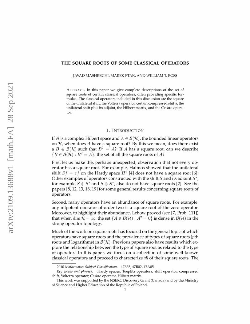
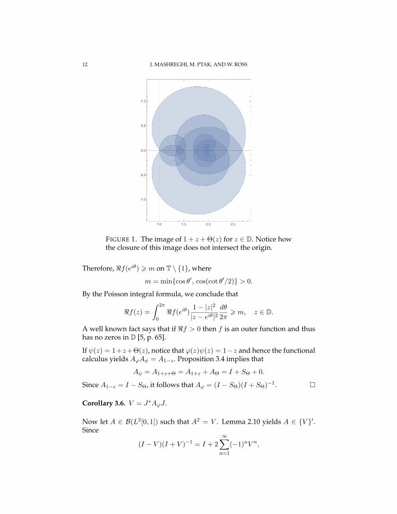
Proof. We first argue that f(z) = 1 + z + Θ(z) is bounded away from zeroon D (see Figure 1) and thus is an invertible element of H∞. Thus ϕ ∈ H∞.Notice that

<f(eiθ) = 1 + cos θ + cos(cot θ/2).

The function cot θ/2 is strictly decreasing on (0, π) as it moves from +∞ tozero, and at θ = π/2 its value is 1. Hence there is a unique θ0 ∈ (0, π/2)such that cot θ0/2 = π/2. Fix any θ′ ∈ (θ0, π/2) and consider the partition(0, π] = (0, θ′) ∪ [θ′, π]. On (0, θ′),

<f(eiθ) = cos θ +

(1 + cos(cot θ/2)

)> cos θ′,

and, on [θ′, π],

<f(eiθ) =

(1 + cos θ

)+ cos(cot θ/2) > cos(cot θ′/2).


FIGURE 1. The image of 1 + z + Θ(z) for z ∈ D. Notice howthe closure of this image does not intersect the origin.

Therefore, <f(eiθ) > m on T \ {1}, where

m = min{cos θ′, cos(cot θ′/2)} > 0.

By the Poisson integral formula, we conclude that

<f(z) =

∫ 2π

0<f(eiθ)

1− |z|2

|z − eiθ|2dθ

2π> m, z ∈ D.

A well known fact says that if <f > 0 then f is an outer function and thushas no zeros in D [5, p. 65].

If ψ(z) = 1+z+Θ(z), notice that ϕ(z)ψ(z) = 1−z and hence the functionalcalculus yields AϕAψ = A1−z . Proposition 3.4 implies that

Aψ = A1+z+Θ = A1+z +AΘ = I + SΘ + 0.

Since A1−z = I − SΘ, it follows that Aϕ = (I − SΘ)(I + SΘ)−1. �

Corollary 3.6. V = J∗AϕJ .

Now let A ∈ B(L2[0, 1]) such that A2 = V . Lemma 2.10 yields A ∈ {V }′.Since

(I − V )(I + V )−1 = I + 2∞∑n=1

(−1)nV n,

SQUARE ROOT 13

then A ∈ {(I − V )(I + V )−1}′. Note that the series above converges innorm since V is quasinilpotent and thus ‖V n‖1/n → 0. From (3.3) we seethat JAJ∗ ∈ {SΘ}′. Thus JAJ∗ = Aψ for some ψ ∈ H∞ (Proposition 3.4).Since

A2ψ = (JAJ∗)2 = JA2J∗ = JV J∗ = Aϕ,

Proposition 3.4 also implies that ψ2−ϕ ∈ ΘH2 +ΘH2. Since ψ2−ϕ belongstoH∞ and must also belong to ΘH∞+ΘH∞, it follows from ΘH∞∩H∞ =C that ψ2 − ϕ ∈ ΘH2. This will imply that ψ2 = ϕ+ Θh for some h ∈ H∞.

Recall that ϕ is an outer function (and hence is zero free in D) and so thereare indeed ψ ∈ H∞ with ψ2 = ϕ. This says that A = J∗AψJ for someψ ∈ H∞ with ψ2 = ϕ+ Θh for some h ∈ H∞.

On the other hand, if ψ ∈ H∞ and h ∈ H∞ with ψ2 = ϕ + Θh, then theoperator J∗AψJ on L2[0, 1] satisfies

(J∗AψJ)2 = J∗A2ψJ = J∗(Aψ +AΘAh)J = J∗(Aϕ + 0)J = J∗AϕJ = V.

Note the use of the H∞ functional calculus for the compressed shift SΘ aswell as the fact thatAΘ = 0 (Proposition 3.4). This argument is summarizedwith the following theorem.

Theorem 3.7. For A ∈ B(L2[0, 1]) the following are equivalent.

(i) A2 = V .

(ii) A = J∗AψJ for some ψ ∈ H∞ such that ψ2 = ϕ+ Θh for some h ∈ H∞.

To show there are only two square roots of V , we follow a variation of anargument of Sarason [24]. Notice that one square root of V is J∗A√ϕJ . Letus show that the other is J∗A−√ϕJ . If B is another square root of V , thenB = J∗AψJ where ψ2 = ϕ+ Θh. In other words, ψ2 − ϕ = Θh. Write

Θh = ψ2 − ϕ = (ψ +√ϕ)(ψ −√ϕ)

and observe that for some γj > 0, the inner functions

q1(z) = exp(− γ1

1− z1 + z

)and q2(z) = exp

(− γ2

1− z1 + z

)divide ψ−√ϕ and ψ+

√ϕ respectively. Moreover, choose the largest γ1, γ2

such that q1 and q2 are inner divisors of ψ −√ϕ and ψ +√ϕ. Write

ψ +√ϕ = q1h1 and ψ −√ϕ = q2h2, h1, h1 ∈ H∞.

It follows that√ϕ = 1

2(q1h1 − q2h2). Since√ϕ is outer, it must be the case

that one of γ1 or γ2 must be zero. If γ1 > 0 and γ2 = 0, then γ1 > 1 andit follows that ψ +

√ϕ is divisible by Θ. An application of Proposition 3.4

yields Aψ = A−√ϕ.


FIGURE 2. The image of z+ Θ(z)(1− z)1/5 for z ∈ D. Noticehow the closure of this image does not intersect the origin.

4. SQUARE ROOT OF A COMPRESSED SHIFT

The previous section leads us to a discussion about the square roots of acompressed shift. For any inner function u, there is the compressed shiftSu = PuS|Ku . The proof of Theorem 3.7 implies the following theorem.

Theorem 4.1. For the atomic inner function Θ and A ∈ B(KΘ), the followingare equivalent.

(i) A2 = SΘ.

(ii) A = Aψ for some ψ ∈ H∞, ψ2 = z + Θh, h ∈ H∞.

Furthermore, SΘ has exactly two square roots.

Proof. First let us prove that the set of square roots of Su is nonempty. Forthis it is enough to check that z + Θ(z)(1 − z)1/5 has no zeros in D (seeFigure 2) and thus has an analytic square root. The reasoning is similar tothe argument in Proposition 3.5, albeit a bit more complex. In this case

f(z) = z + Θ(z)(1− z)1/5

and thus

<f(eiθ) = cos θ + (2 sin θ/2)1/5 cos(θ−π10 − cot(θ/2)

), 0 < θ < π.

SQUARE ROOT 15

There is a similar formula for−π < θ < 0. Then it is enough to observe that

m = inf0<|θ|6π

<f(eiθ) > 0.

By the Poisson integral formula, we conclude that <f(z) > m for all z ∈ D.Thus f is outer and hence has no zeros in D.

Next we observe that A√f is a square root of SΘ. Now follow the argumentused to prove there are only two square roots of the Volterra operator (fol-lowing Theorem 3.7) to prove that the other square root of SΘ is A−√f . �

Not every compressed shift has a square root.

Proposition 4.2. Suppose u is inner and u has a zero at z = 0 of order at leasttwo. Then Su does not have a square root.

Proof. Our earlier discussion shows that the set of square roots of Su are{Aψ : ψ ∈ H∞, ψ2 = z + uh, h ∈ H∞}. If u has a zero of order at least twoat z = 0, then z + uh = z + z2k for some k ∈ H∞ and thus z + z2k(z) hasa zero of order one at z = 0. Thus, there is no H∞ function ψ for whichψ2(z) = z + uh. �

5. SQUARE ROOTS OF Tcos θ .

The Toeplitz operator with symbol cos θ, equivalently

Tcos θ = 12(S + S∗),

is a self-adjoint operator. Therefore, by the spectral theorem for normaloperators, it has a square root.

A result of Hilbert [10] (see [22, Ch. 3] for a modern presentation) showsthat if (un)∞n=0 are the Chebyschev polynomials of the second kind [25],then the operator F : L2(ρ) → H2, where ρ =

√1− x2 on [−1, 1], defined

by

(5.1) Fun =

√π

2zn, n > 0,

is unitary and intertwines Mx on L2(ρ) and Tcos θ. More explicitly,

FMx = Tcos θF.

Thus the matrix representation for Tcos θ with respect to the orthonormalbasis (zn)∞n=0 for H2 is [amn]∞m,n=0, where

amn := 〈Tcos θzn, zm〉H2 , m, n > 0,


which is the Toeplitz matrix

0 12 0 0 0 · · ·

12 0 1

2 0 0 · · ·0 1

2 0 12 0 · · ·

0 0 12 0 1

2 · · ·0 0 0 1

2 0 · · ·...

......

......

. . .

.

By means of the unitary operator F , we can also write

amn =2

π

∫ 1

−1xun(x)um(x)ρ(x)dx, m, n > 0.

This observation gives us a path to describe all of the square roots of Tcos θ.Indeed, if ϕ is any measurable function on [−1, 1] for which ϕ(x)2 = x forall x ∈ [−1, 1], then Mϕ satisfies M2

ϕ = Mx. For example, one can take

ϕ(x) =

{√x if x > 0,

i√−x if x < 0.

Therefore, FMϕF∗ is a square root of Tcos θ. Of course, there are many other

ϕ for which ϕ2 = x. The matrix representations of Mϕ (with respect to theChebyschev basis) and FMϕF

∗ (with respect to the standard basis for H2)are [

2

π

∫ 1

−1ϕ(x)un(x)um(x)ρ(x)dx

]∞m,n=0

.

In fact, these are all the square roots of A.

Theorem 5.2. For B ∈ B(H2) the following are equivalent.

(i) B2 = Tcos θ.

(ii) With respect to the orthonormal basis (zn)∞n=0 ofH2, the matrix representationof B is

(5.3)[

2

π

∫ 1

−1ϕ(x)un(x)um(x)ρ(x)dx

]∞m,n=0

,

where ϕ is a measurable function on [−1, 1] satisfying ϕ(x)2 = x.

Proof. LetB be any fixed square root of Tcos θ. Since Tcos θ is unitarily equiv-alent to Mx on L2(ρ) via the unitary operator F defined by (5.1), the opera-tor F ∗BF is a square root ofMx. By Lemma 2.10, F ∗BF commutes withMx

and thus equal toMϕ for some ϕ ∈ L∞(ρ) (To see why this is true note, thatif AMx = MxA, then Ap = pA(1) for any polynomial p. Letting f ∈ L2(ρ)and selecting polynomials pn → f in norm and, passing to a subsequence,

SQUARE ROOT 17

almost everywhere, we see that Af = (A1)f . This shows that A1 ∈ L∞(ρ)and A is the operator multiplication by A1). This immediately implies

Mx = (F ∗BF )2 = Mϕ2 .

By the uniqueness of the symbol of a multiplication operator, we must haveϕ(x)2 = x. The matrix representation of F ∗BF = Mϕ with respect to the

orthonormal basis (√

2πun)∞n=0 ofL2(ρ) is the same as the matrix representa-

tion of B with respect to the orthonormal basis (zn)∞n=0 of H2, and is givenby (5.3). �

Notice that all of these square roots are complex symmetric operators, sincewith respect to the Chebyschev basis, the matrix representation (5.3) is selftranspose.

6. SQUARE ROOTS OF THE HILBERT MATRIX

The square root of the Hilbert matrix

H =

1 12

13

14 · · ·

12

13

14

15 · · ·

13

14

15

16 · · ·

14

15

16

17 · · ·

......

......

. . .

,

as an operator on `2, involves a similar analysis as with the Toeplitz ma-trix Tcos θ from the previous section. But here, the spectral representationtheorem of Hilbert is replaced by one of Rosenblum [21]. We outline thisanalysis here.

The Laguerre polynomials {Ln(x) : n > 0} form an orthonormal basisfor L2((0,∞), e−xdx). A simple integral substitution shows that the map(Qf)(x) = e−x/2f(x) is unitary from L2((0,∞), e−xdx) onto L2((0,∞), dx).Thus

{QLn = e−x/2Ln(x) : n > 0}is an orthonormal basis for L2((0,∞), dx).

Lebedev [16, 17] proved that if

Kν(z) =

∫ ∞0

e−z cosh(t) cosh(νt) dt,

the modified Bessel function of the third kind, then the operator

(Uf)(τ) =

∫ ∞0

√2τ sinh(πτ)

π√x

Kiτ (x

2)f(x)dx


is a unitary operator from L2((0,∞), dx) to itself. Thus

{wn(x) = UQLn : n > 0}is an orthonormal basis for L2((0,∞), dx). Rosenblum [21] proves that if

(6.1) h(τ) =π

cosh(πτ),

then〈Mhwm, wn〉L2((0,∞),dx) =

1

n+m+ 1, m, n > 0.

This last quantity equals 〈Hem, en〉`2 (the entries of the Hilbert matrix). Insummary, the linear transformation W : `2 → L2((0,∞), dx) defined by

W ({an}n>0) =

∞∑n=0

anwn

is unitary with WHW ∗ = Mh.

As in the previous section, if g ∈ L∞((0,∞), dx) with g2 = h, then Mg isa square root of Mh and thus W ∗MgW is a square root of H . Conversely,if T ∈ B(`2) with T 2 = H , then WTW ∗ is a square root of Mh and hence,as we have seen several times before, WTW ∗ belongs to the commutant ofMh. Since h is a monotone decreasing function on (0,∞), h is injective andhence by a well-known fact about multiplication operators, Mh is cyclic.Since the commutant of a cyclic multiplication operator is the set of mul-tiplication operators Mg on L2((0,∞), dx) with g ∈ L∞((0,∞), dx) we seeas before that T = W ∗MgW , where g2 = h. We therefore arrive at thefollowing theorem. Below, we regard any T ∈ B(`2) as an infinite matrix.

Theorem 6.2. For T ∈ B(`2) the following are equivalent.

(i) T 2 = H .

(ii) There is a measurable function g on (0,∞) with g2 = h, where h is the func-tion from (6.1), such that

T =[ ∫ ∞

0g(x)wm(x)wn(x)dx

]∞m,n=0

.

7. SQUARE ROOTS OF THE CESARO OPERATOR

The Cesaro operator C : H2 → H2 defined by

(Cf)(z) =1

z

∫ z

0

f(ξ)

1− ξdξ, z ∈ D,

is bounded on H2 and a power series computation shows that if f(z) =∑∞j=0 ajz

j ∈ H2, then

(Cf)(z) =∞∑n=0

( 1

n+ 1

n∑j=0

aj

)zn.

SQUARE ROOT 19

Some basic facts about C are found in [1]. With resect to the standard or-thonormal basis (zn)∞n=0 for H2, the matrix representation of C is

(7.1)

1 0 0 0 0 · · ·12

12 0 0 0 · · ·

13

13

13 0 0 · · ·

14

14

14

14 0 · · ·

15

15

15

15

15 · · ·

......

......

.... . .

which is known as the Cesaro matrix. Though not quite obvious, C has asquare root and in fact, one can write them all down - since there are onlytwo of them. This is the topic of this section. It is important to note herethat by the Conway-Olin functional calculus for subnormal operators [3],one can prove that C has at least one square root. The purpose here is toshow that C has exactly two square roots and to specifically write themdown.

Our path to identify the square roots of C is through subnormal operatorsand the work of Kriete and Trutt. Along the way to proving that C is sub-normal, a paper of Kriete and Trutt [14] shows that for w ∈ D, the function

vw(z) = (1− z)w/(1−w)

belongs to H2 and satisfies (I − C∗)vw = wvw. The space

H = {F (z) = 〈f, vz〉H2 : f ∈ H2}defines a vector space of analytic functions on D that becomes a Hilbertspace, in fact a reproducing kernel Hilbert space, when endowed with thenorm ‖F‖H = ‖f‖H2 . This makes the operator (Uf)(z) = F (z) a unitaryoperator from H2 toH. Furthermore,

(U(I − C)f)(z) = 〈(I − C)f, ϕz〉H2

= 〈f, (I − C∗)vz〉H2

= 〈f, zvz〉H2

= z〈f, vz〉H2

= z(Uf)(z)

for all f ∈ H2. Thus, U(I − C) = MzU on H. In summary, C is unitarilyequivalent to M1−z onH.

Thus if A is a square root of C, then, as we have seen with the other oper-ators covered in this paper, A ∈ {C}′ and thus UAU∗ ∈ {M1−z}′ = {Mz}′.So now we need to identify {Mz}′. This will involve the multiplier algebraofH.

Another paper of Kriete and Trutt [15] argues that each ϕ ∈ H∞ is a multi-plier ofH (i.e., ϕH ⊆ H). This is significant since for a general Hilbert space


of analytic functions (the Dirichlet space for example), not every H∞ func-tion is a multiplier. Furthermore, a standard fact that the multiplier algebraof any reproducing kernel Hilbert space of analytic functions on D is con-tained in H∞, along with the observation above, shows that the multiplieralgebra ofH is H∞.

The Hilbert space H also contains the polynomials as a dense set and astandard argument, along with the discussion in the previous paragraph,shows that {Mz}′ = {Mϕ : ϕ ∈ H∞}. Putting this all together, it followsthat if A is a square root of C, then UAU∗ = Mϕ for some ϕ ∈ H∞. But

Mϕ2 = M2ϕ = (UAU∗)2 = UCU∗ = M1−z.

and thus ϕ2 = 1 − z on D. But since ϕ is analytic on D, it must be the casethat ϕ(z) = ±

√1− z. Thus, the Cesaro operator has

U∗M√1−zU and U∗M−√

1−zU

as its only square roots.

The above formulas for the square roots of C are a bit unsatisfying sincethey are hidden behind a unitary operator. Our goal in the next two resultsis to produce a more tangible description of the two square roots ofC. Notethat

√1− z = 1− 1

2z −18z

2 − 116z

3 − 5128z

4 − · · · = 1−∞∑k=1

∣∣∣(12

k

)∣∣∣zk,where the branch of the square root is taken so that

√1 = 1. It is well-

known that∞∑k=0

∣∣∣(12

k

)∣∣∣ <∞.Theorem 7.2. The following are equivalent for A ∈ B(H2).

(i) A2 = C.

(ii)

A = ±(I − 1

2(I − C)− 18(I − C)2 − 1

16(I − C)3 + · · ·),

where the series above converges in operator norm.

Proof. From the above discussion,

U∗M√1−zU and U∗M−√

1−zU

are the only two square roots of C. Since ‖Mz‖ = ‖I−C‖ = 1 [1], the series

I − 12Mz − 1

8M2z − 1

16M3z − · · ·

SQUARE ROOT 21

converges in operator norm to M√1−z . But since Mkz is unitarily equivalent

to (I − C)k, we get

U∗M√1−zU = U∗(I − 1

2Mz − 18M

2z − 1

16M3z − · · ·

)U

= I − 12U∗MzU − 1

8(U∗MzU)2 − 116(U∗MzU)3 + · · ·

= I − 12(I − C)− 1

8(I − C)2 − 116(I − C)3 + · · · .

The other square root of C is computed in a similar way. �

Using an idea of Hausdorff [9], the paper [12] produces all of the lowertriangular square roots of the Cesaro matrix from (7.1). That paper con-siders the Cesaro matrix and its resulting square roots as linear transfor-mations on all one-sided sequences (not necessarily `2 sequences nor anyassumption on the linear transformation being bounded). They show thatall of the lower triangular square roots of the Cesaro matrix are the matricesAσ = [Aσij ]

∞i,j=0, where

(7.3) Aσij =

(i

j

) i−j∑`=0

(−1)`σ(`+ j + 1)1√

`+ j + 1

(i− j`

)i > j,

0 i < j,

and σ : N→ {−1, 1}. One can work out that Aσ equals1 0 0 0 0 · · ·1 −1 0 0 0 · · ·1 −2 1 0 0 · · ·1 −3 3 −1 0 · · ·1 −4 6 −4 1 · · ·...

......

......

. . .

±1 0 0 0 · · ·0 ±

√12 0 0 · · ·

0 0 ±√

13 0 · · ·

0 0 0 ±√

14 · · ·

......

......

. . .

1 0 0 0 0 · · ·1 −1 0 0 0 · · ·1 −2 1 0 0 · · ·1 −3 3 −1 0 · · ·1 −4 6 −4 1 · · ·...

......

......

. . .

,where the sign along the diagonal is determined by the function σ.

They also conjecture that the choices of Aσ, where σ ≡ 1 or σ ≡ −1, are thetwo bounded square roots of the Cesaro matrix (viewed as an operator on`2). This next theorem verifies this conjecture (thus answering a questionposted by Halmos) and also gives an exact description of the square rootsfrom Theorem 7.2.

Theorem 7.4. The following are equivalent for A ∈ B(H2).

(i) A2 = C.

(ii) With respect to the orthonormal basis (zn)∞n=0 for H2, the matrix representa-tion of A is either [Aij ]

∞i,j=0 or −[Aij ]

∞i,j=0, where

Aij =

(i

j

) i−j∑`=0

(−1)`1√

`+ j + 1

(i− j`

)i > j

0 i < j.


Proof. By the above discussion of the results from [12], all of the lower tri-angular square roots of the Cesaro matrix (as viewed as an operator on thespace of all sequences) are of the form Aσ for some σ : N → {−1, 1}. From(7.3), notice that

(7.5) Aσii = σ(i+ 1)1√i+ 1

and so the choice of σ is determined by the entries of Aσ on its diagonal. If

A =(I − 1

2(I − C)− 18(I − C)2 − 1

16(I − C)3 + · · ·),

one of the bounded square roots of the Cesaro matrix from Theorem 7.2,notice that (I − C)k is lower triangular for all k > 0 and thus so is A. Wejust need to determine which choice of σ yields Aσ = A.

The (n, n) entry of I − C is (1 − 1n+1) for n > 0 and since I − C is lower

triangular, it follows that the (n, n) entry of (I − C)k is (1 − 1n+1)k. Thus,

the (n, n) entry of A is

1− 12(1− 1

n+1)− 18(1− 1

n+1)2 − 116(1− 1

n+1)3 − · · · .

But the above is just the Taylor series of√

1− z evaluated at z = 1 − 1n+1

and this turns out to be√

1n+1 . By (7.5), this corresponds to Aσ with σ ≡ 1.

When

A = −(I − 1

2(I − C)− 18(I − C)2 − 1

16(I − C)3 + · · ·),

a similar analysis shows that corresponds to Aσ with σ ≡ −1. �

Thus the only two bounded square roots of the Cesaro (matrix) operatorare

1 0 0 0 0 · · ·1 −1 0 0 0 · · ·1 −2 1 0 0 · · ·1 −3 3 −1 0 · · ·1 −4 6 −4 1 · · ·...

......

......

. . .

1 0 0 0 · · ·0

√12 0 0 · · ·

0 0√

13 0 · · ·

0 0 0√

14 · · ·

......

......

. . .

1 0 0 0 0 · · ·1 −1 0 0 0 · · ·1 −2 1 0 0 · · ·1 −3 3 −1 0 · · ·1 −4 6 −4 1 · · ·...

......

......

. . .

and

1 0 0 0 0 · · ·1 −1 0 0 0 · · ·1 −2 1 0 0 · · ·1 −3 3 −1 0 · · ·1 −4 6 −4 1 · · ·...

......

......

. . .

−1 0 0 0 · · ·0 −

√12 0 0 · · ·

0 0 −√

13 0 · · ·

0 0 0 −√

14 · · ·

......

......

. . .

1 0 0 0 0 · · ·1 −1 0 0 0 · · ·1 −2 1 0 0 · · ·1 −3 3 −1 0 · · ·1 −4 6 −4 1 · · ·...

......

......

. . .

.

SQUARE ROOT 23

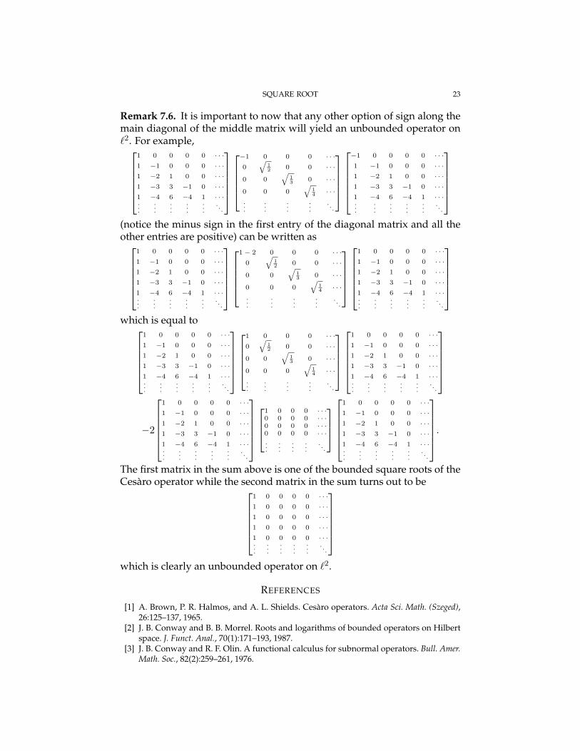
Remark 7.6. It is important to now that any other option of sign along themain diagonal of the middle matrix will yield an unbounded operator on`2. For example,

1 0 0 0 0 · · ·1 −1 0 0 0 · · ·1 −2 1 0 0 · · ·1 −3 3 −1 0 · · ·1 −4 6 −4 1 · · ·...

......

......

. . .

−1 0 0 0 · · ·0

√12 0 0 · · ·

0 0√

13 0 · · ·

0 0 0√

14 · · ·

......

......

. . .

−1 0 0 0 0 · · ·1 −1 0 0 0 · · ·1 −2 1 0 0 · · ·1 −3 3 −1 0 · · ·1 −4 6 −4 1 · · ·...

......

......

. . .

(notice the minus sign in the first entry of the diagonal matrix and all theother entries are positive) can be written as

1 0 0 0 0 · · ·1 −1 0 0 0 · · ·1 −2 1 0 0 · · ·1 −3 3 −1 0 · · ·1 −4 6 −4 1 · · ·...

......

......

. . .

1 − 2 0 0 0 · · ·0

√12 0 0 · · ·

0 0√

13 0 · · ·

0 0 0√

14 · · ·

......

......

. . .

1 0 0 0 0 · · ·1 −1 0 0 0 · · ·1 −2 1 0 0 · · ·1 −3 3 −1 0 · · ·1 −4 6 −4 1 · · ·...

......

......

. . .

which is equal to

1 0 0 0 0 · · ·1 −1 0 0 0 · · ·1 −2 1 0 0 · · ·1 −3 3 −1 0 · · ·1 −4 6 −4 1 · · ·...

......

......

. . .

1 0 0 0 · · ·0

√12 0 0 · · ·

0 0√

13 0 · · ·

0 0 0√

14 · · ·

......

......

. . .

1 0 0 0 0 · · ·1 −1 0 0 0 · · ·1 −2 1 0 0 · · ·1 −3 3 −1 0 · · ·1 −4 6 −4 1 · · ·...

......

......

. . .

−2

1 0 0 0 0 · · ·1 −1 0 0 0 · · ·1 −2 1 0 0 · · ·1 −3 3 −1 0 · · ·1 −4 6 −4 1 · · ·...

......

......

. . .

1 0 0 0 · · ·0 0 0 0 · · ·0 0 0 0 · · ·0 0 0 0 · · ·...

......

.... . .

1 0 0 0 0 · · ·1 −1 0 0 0 · · ·1 −2 1 0 0 · · ·1 −3 3 −1 0 · · ·1 −4 6 −4 1 · · ·...

......

......

. . .

.The first matrix in the sum above is one of the bounded square roots of theCesaro operator while the second matrix in the sum turns out to be

1 0 0 0 0 · · ·1 0 0 0 0 · · ·1 0 0 0 0 · · ·1 0 0 0 0 · · ·1 0 0 0 0 · · ·...

......

......

. . .

which is clearly an unbounded operator on `2.

REFERENCES

[1] A. Brown, P. R. Halmos, and A. L. Shields. Cesaro operators. Acta Sci. Math. (Szeged),26:125–137, 1965.

[2] J. B. Conway and B. B. Morrel. Roots and logarithms of bounded operators on Hilbertspace. J. Funct. Anal., 70(1):171–193, 1987.

[3] J. B. Conway and R. F. Olin. A functional calculus for subnormal operators. Bull. Amer.Math. Soc., 82(2):259–261, 1976.


[4] S. R. Garcia, J. Mashreghi, and W. T. Ross. Introduction to model spaces and their operators,volume 148 of Cambridge Studies in Advanced Mathematics. Cambridge University Press,Cambridge, 2016.

[5] J. Garnett. Bounded Analytic Functions, volume 236 of Graduate Texts in Mathematics.Springer, New York, first edition, 2007.

[6] P. R. Halmos. Ten problems in Hilbert space. Bull. Amer. Math. Soc., 76:887–933, 1970.[7] P. R. Halmos. A Hilbert space problem book, volume 19 of Graduate Texts in Mathematics.

Springer-Verlag, New York-Berlin, second edition, 1982. Encyclopedia of Mathematicsand its Applications, 17.

[8] P. R. Halmos, G. Lumer, and J. Schaffer. Square roots of operators. Proc. Amer. Math.Soc., 4:142–149, 1953.

[9] F. Hausdorff. Summationsmethoden und Momentfolgen. I. Math. Z., 9(1-2):74–109,1921.

[10] D. Hilbert. Grundzuge einer allgemeinen Theorie der linearen Integralgleichungen. ChelseaPublishing Company, New York, N.Y., 1953.

[11] Kenneth Hoffman. Banach spaces of analytic functions. Prentice-Hall Series in ModernAnalysis. Prentice-Hall, Inc., Englewood Cliffs, N. J., 1962.

[12] L. Hupert and A. Leggett. On the square roots of infinite matrices. Amer. Math. Monthly,96(1):34–38, 1989.

[13] D. Ilisevic and B. Kuzma. On square roots of isometries. Linear Multilinear Algebra,67(9):1898–1921, 2019.

[14] T. L. Kriete, III and D. Trutt. The Cesaro operator in l2 is subnormal. Amer. J. Math.,93:215–225, 1971.

[15] T. L. Kriete, III and D. Trutt. On the Cesaro operator. Indiana Univ. Math. J., 24:197–214,1974/75.

[16] N. N. Lebedev. The analogue of Parseval’s theorem for a certain integral transform.Doklady Akad. Nauk SSSR (N.S.), 68:653–656, 1949.

[17] N. N. Lebedev. Some singular integral equations connected with integral representa-tions of mathematical physics. Doklady Akad. Nauk SSSR (N.S.), 65:621–624, 1949.

[18] C. R. Putnam. On square roots of normal operators. Proc. Amer. Math. Soc., 8:768–769,1957.

[19] H. Radjavi and P. Rosenthal. On roots of normal operators. J. Math. Anal. Appl., 34:653–664, 1971.

[20] H. Radjavi and P. Rosenthal. Invariant subspaces. Dover Publications, Inc., Mineola, NY,second edition, 2003.

[21] M. Rosenblum. On the Hilbert matrix. II. Proc. Amer. Math. Soc., 9:581–585, 1958.[22] M. Rosenblum and J. Rovnyak. Hardy classes and operator theory. Oxford Mathematical

Monographs. The Clarendon Press, Oxford University Press, New York, 1985. OxfordScience Publications.

[23] D. Sarason. A remark on the Volterra operator. J. Math. Anal. Appl., 12:244–246, 1965.[24] D. Sarason. Generalized interpolation in H∞. Trans. Amer. Math. Soc., 127:179–203,

1967.[25] Gabor Szego. Orthogonal polynomials. American Mathematical Society Colloquium

Publications, Vol. XXIII. American Mathematical Society, Providence, R.I., fourth edi-tion, 1975.

SQUARE ROOT 25

DEPARTEMENT DE MATHEMATIQUES ET DE STATISTIQUE, UNIVERSITE LAVAL, QUEBEC,QC, CANADA, G1K 0A6

Email address: [email protected]

DEPARTMENT OF APPLIED MATHEMATICS, UNIVERSITY OF AGRICULTURE, UL. BALICKA253C, 30-198 KRAKOW, POLAND.


DEPARTMENT OF MATHEMATICS AND COMPUTER SCIENCE, UNIVERSITY OF RICHMOND,RICHMOND, VA 23173, USA


Documents

THE SQUARE ROOTS OF SOME CLASSICAL OPERATORS