The Sovereign Default Risk of Giant Oil Discoveries*

Carlos Esquivel†

November 9, 2021

Abstract

This paper studies the impact of giant oil field discoveries on default risk. I document

that interest rate spreads of emerging economies increase by 1.3 percentage points following

a discovery of median size. I develop a sovereign default model with investment, production

in three sectors, and oil discoveries. Following a discovery, borrowing increases to finance

investment for oil extraction. Also, capital is reallocated from manufacturing toward the non-

traded sector, which appreciates the real exchange rate and increases the volatility of tradable

income. Higher oil income improves borrowing terms, but higher volatility and borrowing

deteriorate them. With an impatient government, the latter effects dominate. Despite higher

default risk, discoveries generate welfare gains of 2.1 percent. Foregone gains due to govern-

ment impatience are 0.8 percent. Eliminating the volatility of the price of oil has virtually no

effect, but “put” options that insure against low oil prices yield additional gains of 0.5 percent.

(JEL Codes: F34, F41, Q33)

*I am grateful to Manuel Amador and Tim Kehoe for their mentoring and guidance. For comments and discussionsI thank Ana María Aguilar, Cristina Arellano, David Argente, Marco Bassetto, Anmol Bhandari, Javier Bianchi, DavidBradley, Marcos Dinerstein, Doireann Fitzgerald, Stelios Fourakis, Carlo Galli, Salomón García, Eugenia González-Aguado, Pierre-Olivier Gourinchas, Loukas Karabarbounis, Tobey Kass, Todd Keister, Juan Pablo Nicolini, FaustoPatiño, Fabrizio Perri, Agustín Sámano, César Sosa-Padilla, Venky Venkateswaran, and Steve Wu. I also thank seminarparticipants at the Federal Reserve Bank of Minneapolis, the Minnesota Trade Workshop, the Minnesota-WisconsinInternational/Macro Workshop, Rutgers University, the 2019 ITAM alumni conference, the 2020 SED meeting, the2020 Canadian Economics Association virtual meeting, and the EEA 2020 virtual meeting. I acknowledge generoussupport from the Hutcheson-Lilly dissertation fellowship. All errors are my own.

†Assistant Professor at Rutgers University; Email: carlos.esquivel@rutgers.edu; Address: 75 Hamilton St., NewBrunswick, NJ, 08901; Web: https://www.cesquivel.com

1 Introduction

Between 1970 and 2012, sixty-four countries discovered at least one giant oil field, and fourteen

of these countries had a default episode in the following ten years.1 Considering all countries in

the world, the unconditional probability of observing a country default in any given ten year period

was 0.12. Conditional on discovering a giant oil field, this probability was 0.18.2 Hence, a country

that just became richer also became more likely to default on its debt. This paper studies how

the discovery and exploitation of natural resources impact default risk. Following the sovereign

default literature, I focus on emerging economies as they are more prone to default episodes.

I use data of giant oil field discoveries to document the effect of an unexpected large increase

in available natural resources on sovereign interest rate spreads. I build on the work by Arezki,

Ramey, and Sheng (2017), who work with data sets on giant oil discoveries in the world collected

by Horn (2014) and the Global Energy Systems research group at Uppsala University. They use

these data to calculate the net present value of potential future revenues from a discovery relative

to the GDP of the country where it happened. I use this measure of size to estimate the effect of

discoveries on the spreads of 37 emerging economies and find that the effect is large and positive:

spreads increase by up to 1.3 percentage points following a discovery of median size (which is 4.5

percent of GDP). I also estimate the effect of discoveries on the current account, investment, GDP,

and consumption. Following a discovery, these countries run a current account deficit and GDP,

investment, and consumption increase, which is consistent with the findings of Arezki, Ramey,

and Sheng (2017) for a wider set of countries. In addition, I estimate the effects on sectoral invest-

ment and the real exchange rate and find evidence of the Dutch disease: the share of investment

in the manufacturing sector decreases in favor of a higher share of investment in commodities and

non-traded sectors.3 This investment reallocation is accompanied by an appreciation of the real

1A giant oil field contains at least 500 million barrels of ultimately recoverable oil. “Ultimately recoverable re-serves” is an estimate (at the time of the discovery) of the total amount of oil that could be recovered from a field.

2The data of default episodes are from Tomz and Wright (2007) for the years between 1970 and 2004. The defaultprobability conditional on discovery is the probability that a country has a default episode in any of the ten yearsfollowing a discovery.

3The Dutch disease refers to how an increase in natural resource exports induces a reallocation of productionfactors away from manufacturing. Higher revenues from the resource boom increase the demand for all consumptiongoods. This income effect raises the price of non-traded goods, which causes an appreciation of the real exchange rate.This appreciation makes imports of manufactures relatively cheaper and thus induces the reallocation of productionfactors away from this sector into the non-traded sector. The term was first used in 1977 by The Economist to describethis phenomenon in the Dutch economy after the discovery of natural gas reserves in 1959.

1

exchange rate. Arezki, Ramey, and Sheng (2017) find weak evidence of real exchange rate appre-

ciation following oil discoveries for all countries in the world. In contrast, I find that the evidence

is stronger for the 37 emerging economies considered in this paper.

To reconcile these facts, I develop a small-open economy model of sovereign default with

capital accumulation and production in three intermediate sectors: a non-traded sector, a traded

“manufacturing” sector, and a traded “oil” sector. All sectors use capital for production and the

oil sector additionally requires an oil field, which I model as a fixed factor of production. The

economy starts with a small oil field and receives unexpected news about the discovery of a larger

one, which will become productive at a given time in the near future. This lag between discovery

and production is important because the capital and debt accumulation that follow a discovery,

along with uncertainty about the price of oil, are what drive the increase in spreads. In the data,

Arezki, Ramey, and Sheng (2017) find that the average waiting period between discovery and

production is 5.4 years.

After an oil discovery, investment increases so the economy can exploit the larger field when it

becomes productive. The economy runs a current account deficit by issuing foreign debt to finance

investment. Also, there is a reallocation of capital away from manufacturing and toward the non-

traded sector, which is small at first but large once the exploitation of the larger oil field starts.

In the model, as in the data, the price of oil is relatively more volatile than the price of the other

traded goods.4 Higher investment decreases spreads and higher foreign borrowing increases them.

However, the effect of investment is weakened by the reallocation of production capital away from

the manufacturing sector because this reallocation makes tradable income more dependent on oil

revenue and thus more volatile.

I calibrate the model to the Mexican economy, which is a typical small-open economy widely

studied in the sovereign debt and emerging markets literature. Mexico did not have any giant oil

field discoveries between 1993 and 2012, which is the period analyzed in this paper.5 This lack of

discoveries allows me to discipline the parameters of the model with business cycle data that does

4Commodities have always shown a higher price volatility than manufactures. Jacks, O’Rourke, and Williamson(2011) document this stylized fact using data that goes back to the 18th century.

5An interesting case of study would be the Mexican default in 1982, which was preceded by two giant oil fielddiscoveries: one in 1977 and another in 1979, each with an estimated net present value of potential revenues of 50percent of Mexico’s GDP at the time. The main inconvenience is the lack of data on sovereign spreads, which arecrucial to discipline the parameters in the model that control default incentives.

2

not have any variation that could be driven by oil discoveries. Additionally, I use the oil discoveries

data from Arezki, Ramey, and Sheng (2017) to discipline the size and probability of discoveries

in the model. To validate the theory, I generate a panel of model economies and estimate the

responses of macroeconomic variables using the same specification as with actual data.

Under the benchmark calibration, the model generates an increase in sovereign interest rate

spreads of up to 0.5 percentage points following an oil discovery.6 The probability of observing a

default in any ten year window in the model is 0.11. The probability is 0.14 conditional on being

in the ten years after an oil discovery. These values in the data are 0.12 and 0.18, respectively.

Despite the higher frequency of default episodes, oil discoveries generate welfare gains equivalent

to a permanent increase in consumption of 2.1 percent due to the increase in permanent income.

I use the model to perform three counterfactual exercises. For the first counterfactual I consider

a model in which the price of oil is not volatile; I call this the no-price-volatility case. This

exercise illustrates what would happen if the economy was able to costlessly hedge against all

swings in the price of oil. For the second counterfactual I consider an economy with a more

patient government, which virtually eliminates default risk; I call this the patient case. Finally, I

consider an economy in which the government has access to “put” options that allow it to sell its oil

production at a predetermined price, if the realized price of oil is too low, or at the market price for

high realizations; I call this the options case. Oil hedges like these are common practice in private

industries (private oil producers and airlines are usually involved) and the Mexican government

has been a regular participant in these markets since 1990.

In all counterfactual cases, as well as in the benchmark, the economy increases foreign borrow-

ing to finance investment and all three feature capital reallocation. These are the co-movements

that, together with the uncertainty about the price of oil, explain the increase in spreads in the

benchmark case. Default events become more frequent in all but the patient case, in which de-

faults are virtually inexistent. These results stress two important points. First, the frictions in this

economy that explain default events and high spreads are market incompleteness, the lack of com-

6The model abstracts from other complementary forces that could also make spreads increase after an oil discovery.For example, in the presence of growth externalities in the manufacturing sector, the reallocation of capital couldhamper future growth and increase spreads in the present. See Hevia, Neumeyer, and Nicolini (2013) and Alberolaand Benigno (2017) for examples. Also, deterioration of institutions following giant oil discoveries could causespreads to increase. Lei and Michaels (2014) find evidence that giant oil field discoveries increase the incidence ofinternal armed conflicts.

3

mitment from the government, and high borrowing driven by its high relative impatience. Even in

the absence of these frictions, the incentives to borrow to invest in the larger oil field and the in-

centives that drive the reallocation of capital are still present. Second, it is in the presence of these

frictions that the volatility of the price of oil, the choice of borrowing to invest, and the reallocation

of capital together generate an increase in spreads following an oil discovery.

I also compare the welfare gains of oil discoveries in all counterfactual cases with those in the

benchmark. I find that welfare gains remain virtually unchanged in the no-price-volatility case

because losses from higher volatility of consumption are offset by gains from high consumption in

states with high oil prices and not-so-low consumption in states with low oil prices (since default

provides a partial hedge for these low realizations with high debt). I use the patient case to do

a decomposition of welfare gains from oil discoveries and find that there are foregone gains of

0.8 percent due to default risk and high indebtedness driven by government impatience in the

benchmark case. This results favor policies aimed at limiting arbitrary spending of oil revenue

(current and future), like the sovereign wealth funds in Norway (for oil) and in Chile (for copper).

However, implementing such policies may require costly and lengthy institutional reforms, which

may not be feasible when an unexpected giant oil discovery happens. An easier to implement

alternative would be to give the government access to “put” options after an oil discovery. From

the options case I find that this access yields additional gains of 0.5 percent, which are almost as

large as the foregone gains from impatience.

Related literature.—This paper contributes to the literature that studies the role of news as

drivers of business cycles. For an extensive review of this literature see Beaudry and Portier (2014).

This is closely related to the work by Jaimovich and Rebelo (2008) and Arezki, Ramey, and Sheng

(2017). Jaimovich and Rebelo (2008) propose a version of an open economy neoclassical growth

model that generates co-movement in response to unexpected TFP news. They highlight weak

wealth effects on labor supply and adjustment costs to labor and investment as key elements.

Arezki, Ramey, and Sheng (2017) propose a similar model with a resource sector to study the

effects of news shocks in open economies and use data on giant oil discoveries to provide evidence

in favor of the predictions of the model. The model in Section 3 builds on the work in these papers

and contributes by connecting it with the sovereign default literature. To my knowledge, this is the

first paper to study the effect of news on business cycles and default risk in a general equilibrium

4

model with endogenous default.7

This paper also builds on the quantitative sovereign default literature following Aguiar and

Gopinath (2006) and Arellano (2008), which extend the approach developed by Eaton and Gerso-

vitz (1981). They introduce models that feature counter-cyclicality of net exports and interest rates,

which are consistent with the data from emerging markets. Hatchondo and Martinez (2009) and

Chatterjee and Eyigungor (2012) extend the baseline framework to include long-term debt. Their

extensions allow the models to jointly account for the debt level, the level and volatility of spreads

around default episodes, and other cyclical factors.

Gordon and Guerron-Quintana (2018) analyze the quantitative properties of sovereign default

models with capital accumulation and long-term debt. They show that the model can fit cyclical

properties of investment and GDP while also remaining consistent with other business cycle prop-

erties of emerging economies. They also find that capital has non-trivial effects on sovereign risk

but that increased capital almost always reduces risk premia in equilibrium. The model in Section

3 is based on their framework and extends it to have production in different sectors, with one of

them also using natural resources. Arellano, Bai, and Mihalache (2018) document how sovereign

debt crises have disproportionately negative effects on non-traded sectors. They develop a model

with capital, production in two sectors, and one period debt. In their model, default risk makes

recessions more pronounced for non-traded sectors. This is because adverse productivity shocks

limit capital inflows and induce a capital reallocation toward the traded sector to support debt pay-

ments. The model in Section 3 contrasts by featuring two traded sectors and long-term debt. The

effect of sovereign risk on the non-traded sector during recessions also depends on shocks to the

international price of oil and on the current capacity of the oil field. Additionally, news about

future sovereign risk affect current variables due to the long-term nature of the debt.

This paper is closely related to Hamann, Mendoza, and Restrepo-Echavarria (2020). They

study the relation between oil exports, proved oil reserves, and sovereign risk. They use the Insti-

tutional Investor Index (III) as a measure of sovereign risk and document how variations in proved

oil reserves impact the dynamics of the III in oil exporting countries. The shocks these authors

identify are driven by international economic conditions (like oil prices) and by endogenous ex-

7In a related paper, Gunn and Johri (2013) explore how changes in expectations about future default on governmentdebt can generate recessions in an environment where default is exogenous.

5

traction decisions, both of which are the main source of variation in proved oil reserves. There are

three key differences between Hamann, Mendoza, and Restrepo-Echavarria (2020) and the empir-

ical work presented in this paper. The first has to do with the magnitude of the shocks at hand. By

definition, proved reserves do not immediately incorporate giant oil discoveries and the size of their

year-to-year changes is much smaller (see the detailed discussion in Subsection (2.1)). The second

has to do with the fact that, unlike with an increase in proved reserves, newly discovered giant oil

fields cannot be immediately exploited; instead, they require a substantial amount of investment in

subsequent years. Both the size and required investment of discoveries have important implications

on expectations and economic activity. The implied increases in aggregate investment and foreign

borrowing to finance it impact sovereign interest rate spreads in a way that marginal changes in

proved reserves do not. The third is that the nature of the data on oil discoveries allows for a quasi-

natural experiment approach to identify their effect, in contrast to vector autoregressions (VARs)

which require untested identification assumptions and a long time series. The different nature of

the shocks at hand and their economic implications motivate a different theoretical approach as

well. Hamann, Mendoza, and Restrepo-Echavarria (2020) develop a model in which the dynamics

of existing reserves interact with sovereign risk for an implicit fixed stock of capital (i.e., they

abstract from capital accumulation). Reserves increase by random frequent discoveries, which can

be interpreted as additional resources found in existing fields or improvements in extraction tech-

nology that allows to access formerly inaccessible resources (like the introduction of fracking).

In contrast, the model presented in Section 3 allows for capital accumulation and models infre-

quent and much larger oil discoveries to mimic the discovery of new fields that require investment.

This allows the model to study the interaction of sovereign risk with the accumulation of debt and

capital that follow the discovery of giant oil fields.

Finally, this paper relates to the literature that studies the macroeconomic effects of commodity-

related shocks. Hevia and Nicolini (2015) analyze optimal monetary policy in a small-open econ-

omy that specializes in the production of commodities. They find that, due to price and wage

nominal frictions, the Dutch disease generates inefficiencies and full price stability is not optimal.

Ayres, Hevia, and Nicolini (2019) argue that shocks to primary commodity prices account for a

large fraction of the volatility of real exchange rates between developed economies and the US

dollar. They suggest that considering trade in primary commodities could help models generate

6

real exchange rate volatilities that are more in line with the data. The model in Section 3 can be

used as a baseline to study the co-movement of sovereign risk and real exchange rates, which could

point to questions regarding monetary policy in future work.

Layout.—Section 2 describes the data, documents the effect of giant oil discoveries on sovereign

spreads and other macroeconomic aggregates, and discusses the evidence that motivates the theo-

retical framework. Section 3 presents the model. Section 4 describes the calibration, discusses the

main mechanisms in the model, and performs all quantitative analyses. Section 5 concludes.

2 Giant oil discoveries in emerging economies

This section documents the effects of giant oil discoveries on 37 emerging economies considered

in JP Morgan’s Emerging Markets Bonds Index (EMBI).8 Due to data availability, I restrict the

analysis in this paper to these economies and the years between 1993 and 2012. I work with annual

data since the date of oil field discoveries only reports the year of discovery. I use a measure of the

net present value (NPV) of oil discoveries as a percentage of the GDP of the country at the time of

discovery, which was constructed by Arezki, Ramey, and Sheng (2017). I follow their empirical

strategy to estimate the effects of oil discoveries on investment, the current account, GDP, and

consumption. As they do for a larger set of countries, I find evidence for the intertemporal approach

to the current account (as developed by Obstfeld and Rogoff (1995)) and the permanent income

hypothesis.

My contribution is to estimate the effect of giant oil discoveries on the sovereign interest rate

spreads of these economies. I find that spreads increase by up to 1.3 percentage points in the years

following a discovery of median size. This result is robust to controlling for existing proved oil re-

serves, which, as discussed in the following subsection, is a consequence of conceptual differences

between proved reserves and discoveries and also a consequence of the different economic forces

through which these affect default risk. In addition, I estimate the effect of discoveries on the real

exchange rate and investment by sectors and find evidence of the Dutch disease. Subsection 2.1

8The 37 countries are: Argentina, Belize, Brazil, Bulgaria, Chile, China, Colombia, Dominican Republic, Ecuador,Egypt, El Salvador, Gabon, Ghana, Hungary, Indonesia, Iraq, Jamaica, Kazakhstan, Republic of Korea, Lebanon,Malaysia, Mexico, Pakistan, Panama, Peru, Philippines, Poland, Russian Federation, Serbia, South Africa, Sri Lanka,Tunisia, Turkey, Ukraine, Uruguay, Venezuela, and Vietnam.

7

describes the data and the empirical strategy. Subsections 2.3 through 2.5 present the main results

and the Appendix discusses additional details and robustness checks.

2.1 Oil field discoveries and oil reserves

Giant oil discoveries are a measure of changes in the future availability and potential exploitation

of natural resources. Their size is large relative to the GDP of the countries where discoveries

happen, which indicates significant increases in future production possibilities. In order to make

this comparison, Arezki, Ramey, and Sheng (2017) construct a measure of the net present value

(NPV) of giant oil discoveries as a percentage of GDP at the time of discovery as follows:9

NPVi,t =

J∑j=5

qi,t+ j

(1+ri)j

GDPi,t×100 (1)

where qi,t+ j is the annual gross revenue in year t+ j from the field discovered in country i in period

t, ri is the annual discount rate in country i, and GDPi,t is annual GDP of country i at year t. In the

data, there is a time delay of 5.4 years on average between when an oil field is discovered and when

production starts. The annual gross revenue qi,t+ j is derived from an approximated production

profile starting five years after the announcement of the discovery and up to an exhaustion year J,

which is greater than 50 years for a typical giant oil field.10 The data used to estimate the path of

qi,t+ j uses data of “ultimately recoverable reserves” (URR), which is an estimate (at the time of the

discovery) of the total amount of oil that could be eventually recovered from a field given existing

technology.

9They use the data on giant oil discoveries in the world collected by Horn (2014) and the Global Energy Systemsresearch group at Uppsala University. For more details of the construction of the NPV see Section IV.B. in Arezki,Ramey, and Sheng (2017).

10It is important to mention that the gross revenue qi,t+ j considers the same price of oil for subsequent years. Sincethe price of oil closely resembles a random walk, the current price is the best forecast of future prices. See AppendixB of Arezki, Ramey, and Sheng (2017) for a detailed explanation of the approximation of the production profile ofgiant oil discoveries.

8

Figure 1: Distribution of NPV of giant oil discoveries

Percent of GDP, EMBI countries, 1993 –2012.

Considering the 37 economies and the years 1993–2012, there are 61 giant oil field discoveries

in 15 of the 37 countries. The average and median NPV were 18 and 4.5 percent of GDP, respec-

tively. The largest discovery in the sample was in Kazakhstan in 2000 with a NPV of 467. Figure

1 depicts the distribution of the NPV of these discoveries.

As documented by Hamann, Mendoza, and Restrepo-Echavarria (2020), the dynamics of proved

oil reserves have a significant impact on the evolution of credit worthiness of emerging economies

who are oil exporters. In order to understand my findings in light of their results it is important to

note a conceptual distinction between proved oil reserves and URR. There is a range of categories

to measure oil reserves. Figure 2 shows a conceptual diagram from the U.S. Energy Information

Administration that illustrates the differences between these categories.

Figure 2: Oil and natural gas resource categories

Each category implies a different level of uncertainty, where the most certain measure is proved

reserves and the most uncertain is remaining oil and natural gas in-place. Oil and gas in-place refers

to the total amount of resources within a geological formation. Technically recoverable resources

9

includes oil and gas that can be produced based on current technology.11 This is the estimate of

URR that Arezki, Ramey, and Sheng (2017) use to construct the NPV of oil fields, which can be

interpreted as the amount of oil in a field that is physically feasible to extract. Economically re-

coverable resources (ERR) are all URR that can be profitably produced given economic conditions

(like the price of oil and variable costs of production) at the time of measurement. Finally, proved

oil reserves require a higher standard of certainty to be considered profitably and physically recov-

erable. As ERR, proved reserves shrink and grow as the prices of oil and extraction inputs vary,

URR do not.

It is crucial to note that, by definition, the resources contained in giant oil field discoveries are

not included in the measure of proved oil reserves at the time of the discovery. Instead, the oil in

a field is gradually added to proved reserves once drilling starts and new information is collected

about its feasibility and profitability.

Hamann, Mendoza, and Restrepo-Echavarria (2020) document how marginal changes in proved

oil reserves impact the credit worthiness of oil exporting countries, identifying both long and short-

run effects. The shocks these authors identify are driven by international economic conditions (like

oil prices) and by endogenous extraction decisions, both of which are the main source of variation

in proved oil reserves. There are three important differences between Hamann, Mendoza, and

Restrepo-Echavarria (2020) and the work presented in the remainder of this section. The first has

to do with the magnitude of the shocks at hand. By definition, the size of year-to-year changes

in proved reserves is dwarfed by the size of giant oil discoveries. The second has to do with the

fact that newly discovered giant oil fields cannot be immediately exploited; instead, they require

a substantial amount of investment through several years in order to become productive. In con-

trast, proven reserves can be more easily exploited within shorter periods of time. Both the size

of discoveries, and the investment and time they require to become productive have important

implications for expectations and actual economic activity in other sectors, aggregate investment,

and foreign borrowing. These implications impact sovereign interest rate spreads in a way that

marginal changes in proved reserves do not. Finally, as discussed in the next subsection, the nature

of the data on oil discoveries allows for a quasi-natural experiment approach to identify their effect,

11Geophysical characteristics of rocks, as well as physical properties of hydrocarbons (such as viscosity) preventtechnology from producing the entirety of the ultimately recoverable reserves.

10

in contrast to vector autoregressions (VARs) which require untested identification assumptions and

long time series.12

2.2 Empirical strategy and macroeconomic data

As Arezki, Ramey, and Sheng (2017) argue, giant oil discoveries have two unique features that

allow for the use of a quasi-natural experiment approach to identify their effect. First, while policy

and oil prices may drive exploration decisions, the actual timing of discoveries is exogenous due

to uncertainty around oil and gas exploration. Second, there is a time delay of 5.4 years on average

between discovery and production.13 This significant delay allows me to treat giant oil discoveries

as news shocks about future economic conditions.

Following Arezki, Ramey, and Sheng (2017), I estimate the effect of giant oil discoveries on

different macroeconomic variables using a dynamic panel model with a distributed lag of giant oil

discoveries:

yi,t = ρyi,t−1 +10

∑s=0

ψsNPVi,t−s +αi +µt +ξ′X + εi,t (2)

where yi,t is the dependent variable (the dependent variables I will consider are investment, the cur-

rent account, log of real GDP, log of real consumption, sovereign spreads, log of the real exchange

rate, and the share of investment by sector); NPVi,t is the NPV of a giant oil discovery in country i

in year t; αi controls for country fixed effects; µt are year fixed effects; X is a vector of additional

control variables; and εi,t is the error term.14 Country fixed effects control for any unobservable

and time-invariant characteristics, while year fixed effects control for common shocks like world

business cycles and the international price of oil.15

12Additionally, while proved reserves are measured (and vary) periodically, giant oil field discoveries are onlymeasured when they happen, which makes it impossible to identify their effect under the VAR assumptions.

13Arezki, Ramey, and Sheng (2017) mention that experts’ empirical estimates suggest that it takes between four andsix years for a giant oil discovery to go from drilling to production. They also made their own calculation and foundthat the average delay between discovery and production is 5.4 years.

14Also, as Arezki, Ramey, and Sheng (2017) do, I include country-specific quadratic trends for the regressionsof variables yi,t that are non-stationary in the sample. These are GDP, consumption, the real exchange rate, and thespreads. For these variables the augmented Dickey-Fuller test fails to reject a unit root in all countries.

15As noted by Nickell (1981), estimates of a dynamic panel with fixed effects are inconsistent when the time span issmall. He shows that this asymptotic bias is of the order 1/T , which, in the case of the sample considered in this paper,is 0.05. Arellano and Bond (1991) developed an efficient GMM estimator for dynamic panel data models with a smalltime span and large number of individuals. The results in this section are virtually unchanged using the Arellano-Bondestimator. Given the size of the Nickell bias and to keep the results comparable with those of Arezki, Ramey, andSheng (2017) I use the above approach.

11

In my benchmark regressions, the vector X contains contemporaneous and up to ten lags of the

constructed variable Idisc,i,t−s poil,t , where poil,t is the natural logarithm of the international price of

oil at time t and Idisc,i,t−s is an indicator function of whether country i had an oil discovery in period

t− s. The international price of oil is a common shock to all countries; however, the dependent

variables may react differently to this common shock conditional on having had a recent discovery.

These interaction terms control for this. As discussed in the Appendix, these control variables are

only relevant for the estimations of the effects of discoveries on spreads and the real exchange rate.

For consistency, the results presented in this section include these controls in all regressions. The

Appendix shows the results for the specifications without these controls.

As a robustness check in the regression of spreads, I also control for contemporaneous and up

to ten lags of the natural log of proved oil reserves resi,t at year t in country i. Data of proved oil

reserves are from the U.S. Energy Information Administration (EIA) and are measured in billions

of barrels. As can be seen in Subsection 2.4, the results are robust to these controls.

As in Arezki, Ramey, and Sheng (2017)’s analysis, I exploit the dynamic feature of the panel

regression and use impulse response functions to capture the dynamic effect of giant oil discoveries

given by ∆yi,t = ρ∆yi,t−1 +∑10s=0 ψsNPVi,t−s.

My investment, current account, GDP, and consumption data come from the IMF (2013) and

the World Bank (2013). GDP and consumption are measured in constant prices in local currency

units. Investment and the current account are measured as a percentage of GDP. Spreads data

are from JP Morgan’s Emerging Markets Bonds Index (EMBI) Global. The index tracks a value

weighted portfolio of US dollar denominated debt instruments, with fixed and floating-rates, is-

sued by emerging market sovereign and quasi-sovereign entities. Spreads are measured against

comparable US government bonds. The real exchange rate is calculated as RERi,t =ei,tPUS

tPi

twhere

PUSt and Pi

t are the US and country i’s GDP deflators, respectively, and ei,t is the nominal exchange

rate between country i’s currency and the US dollar. These data are also from the IMF (2013).

Finally, the data on investment by sector is in terms of the share of total investment and is from the

United Nations Statistics Division (2017).

12

2.3 Response of macroeconomic aggregates

Figure 3 shows the dynamic response of investment, the current account, GDP, and consumption

to an oil discovery of median size, based on the estimated coefficients of equation (2).16

Figure 3: Impact of giant oil discoveries on macroeconomic aggregates

Impulse response to an oil discovery with net present value equal to 4.5 percent of GDP, which is the median size ofdiscoveries in the sample. The dotted lines indicate 90 percent confidence intervals based on a Driscoll and Kraay(1998) estimation of standard errors, which yields standard error estimates that are robust to general forms of spatialand temporal clustering.

The top left panel shows that the investment-to-GDP ratio increases immediately after an oil

discovery and continues to be higher in the subsequent years. The top right panel shows that

oil discoveries have a negative effect on the current account-to-GDP ratio, which supports the

hypothesis that these countries issue foreign debt to finance higher consumption and investment. In

contrast with the findings in Arezki, Ramey, and Sheng (2017), I find that the current account does

not turn positive even after oil production starts in this subset of emerging economies. As Aguiar

and Amador (2011) argue, governments in highly distorted political environments are unwilling to

reduce their sovereign debt quickly because the value of high immediate consumption outweighs

the cost of debt overhang. The path of the current account in Figure 3 is consistent with these

governments being more impatient and less politically stable than the average governments in the

16The Appendix reports point estimates and their standard errors for the coefficients in equation 2.

13

countries studied in Arezki, Ramey, and Sheng (2017).

The bottom-left panel shows that both GDP and consumption increase after an oil discovery.

However, as Arezki, Ramey, and Sheng (2017) found for a larger set of countries, the estimates for

consumption are very imprecise. This could be a result of substantial measurement error and of

the fact that the consumption variable includes both private and public consumption.

2.4 Effect on sovereign spreads

Figure 4 shows the dynamic response of the spreads following a discovery of median size. The

top left panel shows the response constructed using the estimates from the benchmark regression.

In the year of the discovery, the effect is small and not significantly different from zero. However,

spreads steadily increase in the subsequent years and, by the sixth year after the discovery was

announced, spreads have increased by 1.3 percentage points.

Figure 4: Impact of giant oil discoveries on spreads

Impulse response to an oil discovery with net present value equal to 4.5 percent of GDP, which is the median sizeof discoveries in the sample. The median URR is 1 billion barrels. The dotted lines indicate 90 percent confidenceintervals based on a Driscoll and Kraay (1998) estimation of standard errors, which yields standard error estimatesthat are robust to general forms of spatial and temporal clustering.

This result is robust to controlling for proved oil reserves. The top right panel controls for

the natural logarithm of contemporaneous proved reserves and the bottom left panel controls for

14

this and ten lags. Finally, the bottom right panel uses the natural logarithm of the URR in oil

discoveries as the dependent variable. The evident similarities between these impulse-response

functions suggest that the benchmark result is not sensitive to the particular way of computing

the NPV of discoveries and that it is robust to controlling for proved oil reserves. The Appendix

reports the estimated coefficients for each of these equations. As can be seen there, the coefficients

for proved reserves are positive, which indicates that higher proved reserves are associated with

a deterioration in a country’s credit worthiness, as Hamann, Mendoza, and Restrepo-Echavarria

(2020) document.

These results are striking in the light of the evidence from the previous Subsection and also

in Arezki, Ramey, and Sheng (2017). Income increases during the years following the discovery,

which would indicate that the country has a higher ability to service its debt. However, both

investment and foreign borrowing increase. This suggests that countries still find it preferable to

borrow at higher rates in order to finance the investment that is necessary to exploit the recently

discovered oil field. The theoretical model in Section 3 provides a framework to study how debt

accumulation to finance investment, along with the effects of the Dutch disease, reconcile these

observations.

2.5 Reallocation of capital

Figure 5 shows the dynamic response of the real exchange rate, as well as the share of total in-

vestment in manufactures, commodities, and non-traded sectors.17 Commodities comprise agri-

cultural, fishing, mining and querying activities. The non-traded sector includes construction and

wholesale, retail, and logistics services.

17The estimations for the shares of total investment consider a wider set of countries due to limited data availabilityfor the 37 countries considered in this paper. Their purpose is to support the evidence shown for the estimation of theeffect of discoveries on the real exchange rate, which only considers the aforementioned 37 countries.

15

Figure 5: Impact of giant oil discoveries on sectoral investment and the RER

Impulse response to an oil discovery with net present value equal to 4.5 percent of GDP, which is the median size ofdiscoveries in the sample. The dotted lines indicate 90 percent confidence intervals based on a Driscoll and Kraay(1998) estimation of standard errors, which yields standard error estimates that are robust to general forms of spatialand temporal clustering.

Following a discovery, the share of investment in the manufacturing sector decreases and the

shares in both the commodities and the non-traded sectors increase. The real exchange rate ap-

preciates, which is in line with the theoretical predictions of the Dutch disease: higher income

from the commodity sector increases the consumption of non-traded goods. This in turn increases

the price of non-traded goods and production factors are moved out of manufacturing into non-

traded sectors and resource extraction. Arezki, Ramey, and Sheng (2017) also find (for a larger set

of countries) that the real exchange rate appreciates during the five years following oil discover-

ies; however, their estimates are not significantly different from zero. Figure 5 shows that for the

37 countries studied in this paper, the evidence of appreciation is more conclusive than when all

countries are considered in the same regression, as in Arezki, Ramey, and Sheng (2017).

16

3 Model

This section presents a dynamic small-open economy model in the Eaton and Gersovitz (1981)

tradition with long-term debt, capital accumulation, production in different sectors, and discovery

of natural resources. There is an impatient government that makes borrowing, investment, and

production decisions on behalf of its constituent households and cannot commit to repay its debt.

3.1 Environment

Goods and technology.—There is a final non-traded good used for consumption and capital accu-

mulation. This good is produced with a constant elasticity of substitution (CES) technology that

combines a bundle of an intermediate non-traded good cN,t and two intermediate traded goods:

manufactures cM,t and oil, coil,t :

Yt = A[

ωN (cN,t)η−1

η +ωM (cM,t)η−1

η +ωoil(coil,t

)η−1η

] η

η−1

(3)

where η is the elasticity of substitution, ωi are the weights of each intermediate good i in the

production of the final good, and A is a scaling parameter. Intermediate non-traded goods and

manufactures are produced using capital kN and kM with decreasing returns to scale technologies

yN,t = ztkαNN,t and yM,t = ztk

αMM,t , where zt is a productivity shock that affects both sectors and 0 <

αN < 1, 0 < αM < 1.18 There is a general stock of capital kt that can be freely allocated in these

two sectors within the same period such that kN,t + kM,t = kt .19

Each period, the economy has access to an oil field with capacity nt . To produce oil, the econ-

omy uses the field’s capacity nt and capital koil,t that is specific to the oil sector. The technology to

extract oil is:

yoil,t =

[(1−ζ )

(kαoil

oil,t

)ϕ−1ϕ

+ζ (nt)ϕ−1

ϕ

] ϕ

ϕ−1

(4)

18Decreasing returns to scale captures the presence of a fixed factor, which in this case could be labor (immobilewithin sectors).

19The assumption about the free allocation of capital between the non-traded intermediate sector and manufacturingis made for simplicity. As it will become clear later, what is necessary for my results is that the capital to extract oilis sector specific. Having specific capital in all three sectors would add an additional endogenous state, significantlycomplicating the computation without adding much to the informativeness to the model.

17

where ζ ∈ (0,1) is the weight that corresponds to the oil field, kαoiloil,t is value added in the oil sector,

and ϕ is the elasticity of substitution between value added and the oil field capacity. As with the

other intermediate goods, αoil ∈ (0,1) captures the presence of a unit of labor in the oil sector

that, for simplicity, I assume is supplied inelastically. The key difference between the oil and

the manufacturing sector (the two sources of tradable income in the economy) is that in order to

produce oil the economy needs both capital and an oil field. In the data, capital to extract oil from

an existing field has to be installed on-site. Moreover, capital installed on one field cannot typically

be used to extract oil from a different (newly discovered) field. The CES formulation in equation

(4) allows the model to capture this high degree of complementarity between oil capital and oil

fields.

The resource constraint of the final non-traded good is:

ct + ik,t + ikoil ,t = Yt−Ψ(kt+1,kt)−Ψ(koil,t+1,koil,t

), (5)

where ct is private consumption, ik,t is investment in general capital, ikoil ,t is investment in capital

for the oil sector, Yt is production of the final non-traded good, and Ψ(x′,x) = φ (x′− x)2 is a capital

adjustment cost function.20 The laws of motion for the stocks of capital are:

kt+1 = (1−δ )kt + ik,t (6)

koil,t+1 = (1−δ )koil,t + ikoil ,t (7)

where δ is the capital depreciation rate. As discussed in Subsection 4.4, capital adjustment costs

allow the model to reproduce the anticipation effect in investment observed in the data, that is,

have the economy increase investment before production with the larger oil field starts.

Rest of the world and international prices of goods.—There is a rest of the world economy

where international lenders are and with which the small-open economy trades manufactures and

oil. All prices are expressed in terms of manufactures. I assume that the small-open economy is

small enough so that neither its actions nor its oil discoveries have an effect on the relative price of

20Including capital adjustment costs is important in business cycle models to avoid investment being overly volatile;see Mendoza (1991) for a discussion of the case of small-open economies. Additionally, as Gordon and Guerron-Quintana (2018) show, sovereign default models with capital accumulation require capital adjustment costs to sustainpositive levels of debt in equilibrium.

18

oil. This price is pinned down in the rest of the world and for simplicity I assume it follows some

exogenous stochastic process. As it will be discussed in Subsection 4.4, what is key for the results

in this paper is that the price of oil is relatively more volatile than the price of other traded goods.

For a richer model of the international oil industry see Bornstein, Krusell, and Rebelo (2019).

Shocks and oil discoveries.—The capacity of the oil field can take one of two values nt ∈

{nL,nH} with 0 ≤ nL < nH . The economy starts with nt = nL and with probability πdisc receives

news that its oil capacity will be larger Twait + 1 periods from then, that is nt+Twait+1 = nH . For

simplicity I assume that nt remains high for a stochastic number of periods and with probability

πex it returns to the value nL.21

In each period the economy experiences one of finitely many events st that follow a Markov

chain governed by transition matrix π (st+1|st). This shock is a vector st =(zt , poil,t ,χt

), where

χt ∈ {−1,0,1, ...,Twait +1}. If χt = −1 then nt = nL and the economy has not discovered an oil

field yet. If χt = 0...Twait then nt = nL but there was news of a giant oil field discovery in period

t− χt . Finally, if χt = Twait +1 then nt = nH . When χt =−1, then Pr (χt+1 = 0|χt =−1) = πdisc

is the probability of an oil discovery. For χt = 0, ...,Twait this variable keeps track of the time

between discovery and production, which is exogenously given by the value of Twait and thus

Pr (χt+1 = χt +1|0≤ χt ≤ Twait) = 1.22

Preferences.—The government has preferences over private consumption ct represented by

E0[∑

∞t=0 β t

Gu(ct)], where u(c) = c1−σ−1

1−σand βG is the government’s discount factor. As is standard

in the sovereign default literature, I model the government as a relatively impatient agent. In

particular, I assume that the government’s discount factor is smaller than the discount factor of the

households βG < βHH .23 In Subsection 4.5 I analyze the implications that this assumption has on

21The average duration of a giant oil field is 50 years, which will be the calibration target for πex. This is much longerthan the time-span in the data in section 2.1. Moreover, as Arezki, Ramey, and Sheng (2017) document, the productionrate is highest for the initial years after the field becomes productive and then decreases at a slow rate. A richer modelof oil production would include details on the depletion of the reserves on the field through its exploitation, like themodel in Hamann, Mendoza, and Restrepo-Echavarria (2020). However, the focus of this paper is on the effect ofoil discoveries and the transition between discovery and production, rather than on the cyclical implications of theexploitation of existing oil fields.

22Given this formulation, χ captures both the news shock and keeps track of the time between news and production.Unlike Arezki, Ramey, and Sheng (2017), I assume the oil field takes two values rather than allowing for richerdepletion dynamics. This is a simplifying assumption made for computational tractability because, unlike the modelin Arezki, Ramey, and Sheng (2017), the model presented here requires a global solution in order to accurately computedefault probabilities.

23There is a vast political economy literature that provides models that rationalize impatient policy makers. Forexamples with external sovereign debt see Cuadra and Sapriza (2008), Aguiar and Amador (2011), and Amador

19

spreads after an oil discovery and on the welfare gains of oil discoveries.

Debt structure.—The government issues long-term bonds that mature probabilistically at a

rate γ . The law of motion of bonds is:

bt+1 = (1− γ)bt + ib,t (8)

where bt is the number of bonds due at the beginning of period t and ib,t is the amount of bonds

issued in period t.24 The bonds are denominated in terms of the numeraire good (manufactures).

Default, repayment, and the balance of payments.—At the beginning of every period the

government has the option to default. If the government defaults it gets excluded from international

financial markets—although it can still trade in goods—for a stochastic number of periods; the

government gets re-admitted to financial markets with probability θ and zero debt. While in default

productivity is zdt ≤ zt . More specifically, I assume an asymmetric penalty to productivity so that

zdt = zt −max

{0,d0zt +d1z2

t}

, where d0 < 0 < d1. This implies that the productivity penalty is

zero when zt ≤ −d0d1

and rises more than proportionately when zt > −d0d1

. This asymmetry in the

default penalty is crucial in generating default dynamics that are in line with the data in this class of

models, in particular the counterciclicality of spreads and the current account (see the discussions

in Arellano (2008) and Chatterjee and Eyigungor (2012)).25

In default, the balance of payments is:

0 = xM,t + poil,txoil,t (9)

where xM,t = yM,t − cM,t and xoil,t = yoil,t − coil,t are net exports of manufactures and oil, respec-

tively. Equation (9) implies that in default trade in goods has to be balanced; imports to increase

consumption of a traded good have to be financed by exports of the other traded good.

If the government decides to pay its debt obligations then it has access to international financial

(2012, Working Paper.).24For a similar formulation see Hatchondo and Martinez (2009), Arellano and Ramanarayanan (2012), and Chatter-

jee and Eyigungor (2012).25Mendoza and Yue (2012) develop a general equilibrium model of sovereign default and business cycles in which

default can endogenously trigger an efficiency loss similar to the one captured by zdt .

20

markets and can issue new debt ib,t . In this case, the balance of payments is:

γbt = xM,t + poil,txoil,t +qt (bt+1− (1− γ)bt) (10)

where qt is the price of newly issued debt. Equation (10) shows how payments of debt obligations

(left-hand side) are supported by net exports of goods and by the issuance of new debt.

Lenders.—The bonds issued by the government are purchased by a large number of risk-

neutral foreign lenders. I assume these lenders have deep pockets and behave competitively. Also,

lenders have access to a one-period risk-free bond that pays a fixed interest rate r?, which represents

the lenders’ opportunity cost of holding government debt for one period.

3.2 Recursive formulation and timing

The state of the economy is the underlying stochastic variable s, the stock of general capital k,

the stock of capital for the oil sector koil , the outstanding government debt b, and an indicator of

whether the government is in default or not.

The government.—Let V (s,k,koil,b) be the value of the government that starts the period not

in default. I follow the Eaton and Gersovitz (1981) timing and assume that the government first

chooses whether to repay its debt obligations, d = 0, or to default, d = 1:

V (s,k,koil,b) = maxd∈{0,1}

{[1−d]V P (s,k,koil,b)+dV D (s,k,koil)

}where V P (s,k,koil,b) is the value of repaying and V D (s,k,koil) is the value of default.26

If the government decides to default then its debt obligations are erased and it gets excluded

from financial markets. Then, the government simultaneously chooses the stocks of capital next

period k′ and k′oil , static allocations of general capital in manufactures and the non-traded interme-

diate sector K = {kN ,kM}, net exports of manufactures and oil X = {xM,xoil}, and consumption of

final and intermediate goods C = {c,cN ,cM,coil} to solve:

V D (s,k,koil) = max{k′,k′oil ,C,K,X}

{u(c)+βGEs′|s

[θV(s′,k′,k′oil,0

)+(1−θ)V D (s′,k′,k′oil

)]}26Alternative timing assumptions can give rise to multiplicity of equilibria like, for example, the one introduced by

Cole and Kehoe (2000). For detailed discussions and literature surveys on this topic see Aguiar and Amador (2014)and Aguiar, Chatterjee, Cole, and Stangebye (2016).

21

subject to the resource constraint of the final good (5), the resource constraint of general capital

kt = kN + kM, the laws of motion of capital (6) and (7), the resource constraints of intermediate

goods cN = yN , cM + xM = yM and coil + xoil = yoil , and the balance of payments under default

(9). Note that the government can trade in goods, but trade has to be balanced since it cannot issue

debt.

If the government decides to repay then it simultaneously chooses the stocks of capital k′ and

k′oil , and debt b′ for the next period, static allocations of general capital in manufactures and the

non-traded intermediate sector K = {kN ,kM}, net exports of manufactures and oil X = {xM,xoil},and consumption of final and intermediate goods C = {c,cN ,cM,coil} to solve:

V P (s,k,koil,b) = max{k′,k′oil ,b

′,C,K,X}

{u(c)+βGE

[V(s′,k′,k′oil,b

′)]}subject to the resource constraint of the final good (5), the resource constraint of general capital

kt = kN +kM, the laws of motion of capital (6) and (7), the law of motion of bonds (8), the resource

constraints of intermediate goods cN = yN , cM + xM = yM and coil + xoil = yoil , and the balance of

payments under repayment (10).

Lenders.—In each period, if the government is in good financial standing it makes its borrow-

ing and investment decisions simultaneously. Then, lenders observe these decisions and purchase

the bonds. Since lenders behave competitively, the equilibrium price of bonds is such that lenders

make zero profits in expectation. Given that the lenders are risk-neutral they price the bonds ac-

cording to:

q(s,k′,k′oil,b

′)= Es′|s{[

1−d(s′,k′,k′oil,b

′)][γ +(1− γ)q(s′,k′′,k′′oil,b

′′)]}1+ r?

(11)

where k′′, k′′oil and b′′ are lenders’ expectations about the government’s investment and borrowing

policies in the following period.

An important assumption in this environment is that all of the government’s dynamic decisions

are made simultaneously, in other words, both investment and indebtedness are contractible. This

implies that next-period capital is an argument of the price function in (11). In a recent paper Galli

(2019) studies an environment in which investment is not contractible. In that case the price func-

tion does not depend on next-period capital and multiple equilibria with high and low investment

22

may arise.

3.3 Equilibrium

A Markov equilibrium is value functions V , V D, and V P; policy functions for capital in default kD

and kDoil; policy functions for capital and debt in repayment, k, koil , and b; a default policy function

d; policy functions for static allocations in repayment and in default; and a price schedule of bonds

q such that: (i) given the price schedule q, the value and policy functions solve the government’s

problem, (ii) the price schedule satisfies (11), and (iii) lenders have rational expectations about

the government’s future decisions, that is k′′ = k(s′,k′,k′oil,b

′), k′′oil = koil(s′,k′,k′oil,b

′), and b′′ =

b(s′,k′,k′oil,b

′) in equation (11).

4 Quantitative analysis

4.1 Model solution

I solve the functional equations of the government’s problem and of the price of bonds using value

function iteration. Following Hatchondo, Martinez, and Sapriza (2010), I compute the limit of the

finite-horizon version of the economy. To solve for the optimal investment and debt issuance I use

a nonlinear optimization routine taking the current state as an initial guess.27 The value functions

V D and V P and the price schedule for bonds q are approximated using linear interpolation. I use 25

grid points for bonds, capital, oil capital, productivity shocks, and shocks to the price of oil. See

Appendix B for more details of the implementation of this algorithm to the model in the previous

section.27In the presence of convex capital adjustment costs, the policy functions for capital are not too far away from the

45 degree line, which makes the current state a good initial guess. The algorithm is robust to using any value for thedebt policy as an initial guess. The code used to compute the solution of the model is written in the Julia language.I use the Nelder-Mead algorithm from the Optim.jl package, which follows the gradient free non-linear optimizationalgorithm developed by Nelder and Mead (1965).

23

4.2 Calibration

I calibrate the model to the Mexican economy using the period 1993–2012.28 There are two reasons

that make Mexico an ideal example for the purposes of this paper. The first is that Mexico has been

widely studied in the sovereign debt literature because its business cycle has the same properties as

other emerging economies (see for example Aguiar and Gopinath (2007), and Aguiar, Chatterjee,

Cole, and Stangebye (2016)). In addition, as noted by Bianchi, Hatchondo, and Martinez (2018),

Mexico gives calibration targets for average levels of debt and spreads that are close to the median

value for emerging economies. In short, Mexico is a typical emerging economy. The second

desirable property is that Mexico did not have any giant oil field discoveries during the period

of study. This lack of discoveries allows me to discipline parameters of the model with business

cycle data that do not include variation in endogenous variables induced by giant oil discoveries.

This property is important because in the following subsection I validate the model by simulating

a panel of economies and running the same regressions as in Section 2.

A period in the model is one year.29 There are two sets of parameters: the first (summarized

in table 1) is calibrated directly and the second (summarized in table 2) is chosen so that moments

generated by model simulations match their data counterparts. I set the capital shares to αN = 0.66

and αM = 0.57 following Mendoza (1995). I set the share of oil rent to ζ = 0.38 and the capital

share in the value added of the oil sector to αoil = 0.49 as in Arezki, Ramey, and Sheng (2017).

For the elasticity of substitution between oil and field capacity I set ϕ = 0.4, which implies a

high level of complementarity between these to factors.30 I use data on sectoral GDP for Mexico

between 1993 and 2012 to estimate the elasticity of substitution η = 0.74.31 I set the weights

ωN = 0.60, ωM = 0.34, and ωoil = 0.06 using aggregate consumption shares. I set the relative risk

aversion parameter to σ = 2, the capital depreciation rate to δ = 0.05, and the risk free interest

rate to r? = 0.04, which are standard values in the international macroeconomics literature. I set28Except for the spreads data, which starts in 1998 for Mexico.29This is to be consistent with the empirical work from Section 2, which is limited to a yearly frequency since this

is the scope of the oil discoveries data.30To my knowledge, there is no empirical guidance applicable to a macroeconomic model regarding this level of

complementarity. The results discussed in the remainder of the paper are not sensibly altered by different values ofthis parameter.

31To estimate the elasticity of substitution I follow the methodology used by Stockman and Tesar (1995). Asdiscussed by Mendoza (2005) and Bianchi (2011), the range of estimates for the elasticity of substitution betweentradables and non-tradables is between 0.40 and 0.83.

24

the household’s discount factor to be βHH = 11+r? , that is, I assume households are as patient as the

foreign lenders. This parameter will be important for the welfare calculations in Subsections 4.5

and 4.6.

I assume the productivity shock follows an AR(1) process logzt = ρz logzt−1+σzεz,t , where εz,t

are iid with a standard normal distribution. I set the persistence to ρz = 0.91 and standard deviation

σz = 0.02, which are standard values in the literature, and use these values to approximate the

process with a finite state Markov-chain using the method proposed by Tauchen (1986).

I assume that the price of oil also follows an AR(1) process log poil,t = (1−ρoil) log poil +

ρoil log poil,t−1 +σpεoil,t , where εoil,t are iid with a standard normal distribution, νp is the stan-

dard deviation, ρoil is the persistence parameter, and poil is the mean of the price of oil normal-

ized in the model to poil = 1. To estimate the persistence and standard deviation I use data of

the average price of crude oil from the World Bank Commodity Price Data between 1993 and

2012. The source includes monthly data of the average of the Brent, Dubai, and West Texas In-

termediate prices. I take the yearly average and divide by the US GDP deflator in each year to

calculate a yearly series of the real price of oil. I take the first difference of the above equation,

∆ log poil,t = ρoil∆ log poil,t−1 +σpεoil,t , and estimate that the persistence parameter is ρoil = 0.92

and the standard deviation of the iid shock is σp = 0.18. I use these estimates to approximate the

process with a finite state Markov-chain using the Tauchen method and normalizing poil = 1.

25

Table 1: Parameters calibrated directly from the data

Parameter Value Source

capital shares

αN 0.66Mendoza (1995)

αM 0.57

αoil 0.49Arezki, Ramey, and Sheng (2017)

oil rent ζ 0.38

elasticity of substitution η 0.74 estimated for Mexico

intermediate ωN 0.60

output ωM 0.34 shares in aggregate consumption

shares ωoil 0.06

risk aversion σ 2.00

standard valuescapital depreciation rate δ 0.05

risk free rate r∗ 0.04

household’s discount factor βHH 0.96 as impatient as foreign lenders

bonds maturity rate γ 0.14 7 year average duration

probability of reentry θ 0.40 2.5 years exclusion

probability of discovery πdisc 0.01 probability of discoveries in the data

probability of exhaustion πex 0.02 average field life of 50 years

waiting time for field to be available Twait 5 average lag in the data

persistence of price of oil ρoil 0.92 AR(1) estimation for

volatility of price of oil σp 0.18 the real price of oil

persistence of productivity ρz 0.91 standard

volatility of productivity σz 0.02 values

size of small oil field nL 0.35 steady state oil net exports=1% of GDP

size of large oil field nH 0.51 steady state NPV of discovery=18% of GDP

scaling parameter A 0.84 steady state final good production = 1

26

I set the probability of re-entry to financial markets to θ = 0.40, so that the average duration of

exclusion is 2.5 years, following Aguiar and Gopinath (2006). I set γ = 0.14 so that the average

duration of bonds is 7 years, as documented for Mexico by Broner, Lorenzoni, and Schmukler

(2013).

To calibrate some parameters I need to compute nominal and real GDP. In the model, nominal

GDP in period t is GDPt = PtYt +xM,t + poil,txoil,t , where Pt is the standard CES price index for the

production function in equation 3. To be consistent with national accounts for Mexico, I compute

real GDP using base period prices RGDPt = P0Yt +xM,t + poil,0xoil,t , where t = 0 is the base period.

I define the GDP deflator in the model to be pt =GDPt

RGDPtand the real exchange rate to be 1

pt.

I calibrate the scaling parameter A and the size of the oil field before discovery nL jointly using

the steady state of the economy with no debt and all shocks set equal to their mean values. I set

A = 0.84 and nL = 0.35 so that in the steady state production of the final good is Yss = 1 and net

exports of oil are 1% of GDP xoil,ssGDPss

= 0.01 (which is the average for Mexico between 1993 and

2012).

I set the probability of an oil discovery to πdisc = 0.01, which is the probability of new dis-

coveries observed in the data after excluding subsequent discoveries in the same country.32 I set

the waiting time between discovery and production to Twait = 5, which is the average lag observed

in the data, and the probability of exhaustion to πex = 0.02 for an average life of 50 years for a

discovered large field.

The net present value of an oil discovery as a percentage of nominal GDP in the steady state is:

NPVss = 100∗∑

50s=0

(1

1+rss

)s+Tdisc+1poil,ss

[f oil (koil,ss,nH

)− f oil (koil,ss,nL

)]GDPss

where poil,ss = zss = 1 and rss = 0.069 is the interest rate consistent with a target for spreads of

2.9% (see Table 2 below). This calculation is akin to the calculation made by Arezki, Ramey, and

Sheng (2017) with actual data following equation (1). I set nH = 0.51 so that NPVss = 18%, which

is the average NPV of the discoveries studied in Section (2).

Table 2 summarizes the parameters calibrated by simulating the model. This calibration con-

32I consider oil discoveries in countries that had not had a discovery in the previous 6 years. The reason to do this isthat the model does not accommodate subsequent discoveries. The unconditional probability of discovery in the datais 0.045. The main results of the paper remain unchanged if this probability was used instead.

27

siders 50 periods of 100 simulated economies in their ergodic state with n= nL. That is, economies

in their ergodic state without any oil discoveries during the sampled period, like Mexico in the data.

Table 2: Parameters calibrated simulating the model

Parameter Value Parameter Value

discount factor β 0.8775 default cost d0 -0.16

capital adjustment cost φ 2.0 default cost d1 0.222

Moment Data Model

average spread (percentage) 2.9 2.7

σcons/σGDP 1.0 1.1

σinv/σGDP 3.0 3.1

public external debt-to-GDP ratio 0.15 0.14

Moments are computed by generating 100 samples of 550 periods and considering only the last 50 observations. Onlysamples with no oil discoveries in the last 50 periods are considered.

There are four parameters chosen to match four moments from the data: the average spreads,

the volatility of consumption relative to the volatility of GDP, the volatility of investment relative

to the volatility of GDP, and the public external debt-to-GDP ratio. The value of the discount factor

β mainly determines the debt-to-GDP ratio; average spreads and relative consumption volatility

are mainly pinned down by the default cost parameters d0 and d1; and the relative volatility of

investment is mostly determined by the capital adjustment cost parameter φ . Spreads data are

from the EMBI (same as in Section 2).

Spreads in the model are computed as the difference between the interest rate implied by the

price of government bonds qt and the risk free rate rt − r?, where rt =γ−γqt

qt. Data of external

public debt-to-GDP ratio are from the World Bank (2013). The debt-to-GDP ratio in the model

is computed as the ratio of the stock of debt to nominal GDP btGDPt

. For the relative volatility

of consumption and investment I use HP-filtered data of the log of real consumption, investment

and GDP from Mexican national accounts and compute the standard deviation of their cyclical

components. In the model, I compute real consumption, investment, and GDP by dividing by the

GDP deflator Ptctpt

,Pt(it+ioil,t)

pt, and PtGDPt

pt. I apply the HP-filter to the log of the series and compute

the standard deviation of the cyclical components.

28

The following subsection shows the model’s predictions after an oil discovery, with special

focus on the model’s ability to reproduce the responses documented from the data in Section 2.

4.3 Model fit

Default episodes after oil discoveries.—As mentioned in the introduction, the data of default

episodes in Tomz and Wright (2007) show that the unconditional probability of observing a country

default in any given ten-year period is 0.12.33 Considering only ten-year periods that follow a

giant oil discovery, this probability is 0.18. In the model these probabilities are 0.11 and 0.14,

respectively. To compute the model probabilities I simulate an economy for 100,500 periods, drop

the first 500, and use the data for all default episodes and those that happen in the 10 years that

follow an oil discovery.

Non-targeted business-cycle moments.—Table 3 shows business-cycle moments that are not

targeted. The model does a good job in generating counter-cyclical trade balances and current

accounts, as well as their relative variances vis-a-vis GDP. The model generates spreads that are

slightly less volatile than those in the data.34

Table 3: Untargeted moments

Moment Data Model

st. dev. of spreads (percentage) 1.3 0.7

σT B/σGDP 0.5 0.6

σCA/σGDP 0.5 0.9

corr( CA

GDP ,GDP)

-0.6 -0.4

corr( T B

GDP ,GDP)

-0.3 -0.4

Moments are computed by generating 100 samples of 550 periods and considering only the last 50 observations. Onlysamples with no oil discoveries in the last 50 periods are considered.

Estimated responses to oil discoveries.—In order to assess the model’s ability to explain the

responses to oil discoveries observed in the data, I simulate a panel of economies and run the same

33I calculate this probability as 1 − Pr (no default in 10 years), where Pr (no default in 10 years) =

[1−Pr (default in a year)]10.34In the model, the current account is defined as the change in the net foreign asset position, which is cat =

−(bt+1−bt).

29

regressions as in Section 2.

The model-generated panel data consist of 50 periods and 100 economies. Each economy

i= 1...100 is simulated for 550 periods and then the first 500 periods are dropped to remove any de-

pendence from initial conditions. All 100 economies face the same shocks to oil prices{

poil,t}550

t=1

and are ex-ante identical. Heterogeneity arises from different realizations of productivity shocks

zi = {zi,t}550t=1 (which generate different choices

(di,t ,ki,t ,koil,i,t ,bi,t

)) and, most importantly, be-

cause some economies experience oil discoveries during the sample period and some do not. If

economy i discovers an oil field in period t, I compute the net present value NPVi,t as:

NPVi,t = 100∗

50∑j=0

(1

1+ri,t

)s+Tdisc+1poil,t

[f oil (koil,i,t ,nH

)− f oil (koil,i,t ,nL

)]GDPi,t

where ri,t =γ−γqi,t

qi,tis the interest rate that country i faces in period t, with qi,t =

q(

si,t ,k′i,t ,k′oil,i,t ,b

′i,t

). Note that even though nH and nL are fixed, there is vast heterogeneity in

the NPVi,t generated by the model. This is because, by construction, the NPVi,t (both in the model

and in the data) is not only a measure of the quantity of oil in the ground, but also a measure of

the relative increase in permanent income that the discovery implies for the country in question.

For instance, a discovery when the price poil,t is relatively high will have a much larger net present

value than when the price is low. Similarly, a discovery in a country with relatively high default

risk (high ri,t) will have a lower net present value because high interest rates hamper the country’s

ability to transform income from future oil revenues into present consumption.

I use the model simulated data to estimate the coefficients in equation (2) using spreads, total

investment, the current account, the real exchange rate, GDP, and consumption as dependent vari-

ables. I then use these coefficients to construct impulse-response functions like the ones in Figures

3, 4, and 5.

Figure 6 compares the impulse-response functions estimated with model and actual data. The

model’s ability to qualitatively reproduce these untargeted responses is remarkable. Following a

discovery, spreads steadily increase and peak around the year when production starts. Investment

immediately increases and this increase is accompanied by a current account deficit of similar

magnitude. The real exchange rate appreciates and both GDP and consumption increase.

30

Figure 6: Impulse-response functions to a giant oil discovery of median size

The solid blue lines correspond to the data, where the median net present value of oil discoveries is 4.5 percentof GDP. The dotted orange lines correspond to the model, where the median and average net present value of oildiscoveries is 18 percent of GDP.

Quantitatively, however, the responses of spreads and the real exchange rate in the model fall

short, while the responses of GDP and consumption are overstated. It is important to note that the

main objective of this quantitative exercise is not to adjust the model to exactly fit these responses,

but rather to asses if the directions of the responses jointly generated by the model are consistent

with those from the data.35 The remainder of this subsection discusses some possible explanations

for the main quantitative discrepancies and points to inefficiencies that are not present in the model

35For example, lower GDP, lower spreads, lower investment, or a real exchange rate depreciation would be moreconcerning results.

31

that could reconcile them. However, exploring the plausibility and quantitative implications of

such inefficiencies is beyond the scope of this paper since they would amplify an effect that the

parsimonious model from Section 3 already captures.

In the data, spreads increase by up to 1.3 percentage points, but only by up to half a percentage

point in the model. It is important to note that the model data is a panel of the same country in

different states (a “panel of Mexicos” with different histories of shocks). In the data, however,

there is richer heterogeneity related to the primitives of the economy (countries face different

productivity processes and may have governments with different levels of impatience and different

costs to default). While Mexico is indeed a typical emerging economy, these other dimensions of

heterogeneity could introduce higher responses of spreads. Also, the government in the model has

the ability to exactly pin down all investment and borrowing allocations, which in turn affect the

interest rate the government faces. If investment was chosen by the private sector there could be

a pecuniary externality from private investors not internalizing the effect that their decisions have

on the interest rates that the government faces. This inefficiency could also amplify the response

of spreads.

In the model, the real exchange rate is the reciprocal of the GDP deflator pt . In both the model

and the data the real exchange rate appreciates following an oil discovery. This response is a result

of the reallocation of production factors from manufacturing to non-traded sectors. In the data the

appreciation is smother than in the model, where most of the appreciation happens once the larger

oil field becomes available. This is a direct implication of the assumption that capital can be freely

reallocated from the manufacturing sector to the non-traded sector within the same period.

Regarding GDP, the increase in the model is moderate the years right after a discovery is

announced and much larger once production in the oil field starts. This is consistent with what

Arezki, Ramey, and Sheng (2017) find in the data for a larger set of countries. The fact that GDP

increases right away for the sample of emerging economies considered in this paper is puzzling

and a direction for future work. The response of GDP in the model is also much larger than

the response in the data. One possible reason for this large effect could be due to inelastic labor

supply. Arezki, Ramey, and Sheng (2017) find that hours decline following oil discoveries, which

could be generated by a model with separable preferences for leisure. In addition, an environment

with rent-seeking agents running the government like the one studied in Tornell and Lane (1999)

32

could generate a lower response of GDP. In their model, a “voracity effect” generates a more-

than-proportionate increase in rent-extracting fiscal redistribution as a response to a terms of trade

windfall. This redistribution hampers investment and limits GDP growth.

Finally, consumption in the model starts increasing only after production in the oil field starts,

while the data show weak evidence of any movement at all.36 On average, the government in

the model cannot smooth consumption too much before production starts because the debt level

is already too high in the ergodic state. In other words, borrowing to consume is already too

expensive.

4.4 Discussion of assumptions and mechanism

There are four key assumptions in the model that allow it to produce similar responses to oil dis-

coveries as we observe in the data: (i) capital adjustment costs, (ii) production of non-traded goods,

(iii) high volatility of the international price of oil, and (iv) long-term debt. This Subsection dis-

cusses how these assumptions shape the mechanism through which spreads increase following an

oil discovery, which can be summarized as follows. After an oil discovery, because of capital ad-

justment costs, the government borrows to invest in capital for the oil sector. Borrowing increases

spreads and investment reduces them. However, the former effect dominates because, once the

large oil field is being exploited, capital will be drawn away from the manufacturing sector. This

reallocation will make tradable income—used to support debt payments—more dependent on oil

revenue and thus more volatile. With long-term debt, this higher volatility of future income (as

well as higher future borrowing) affects the spreads in all the preceding periods, starting with the

period when the information of a discovery arrives and being more affected once production in the

new field is about to start.

Throughout this Subsection, I use the equilibrium policy functions and price defined in Subsec-

tion 3.3 that result from the calibration described in Subsection 4.2. I look at the path of different

endogenous variables in the twenty periods following an oil discovery. For illustrative purposes,

I fix the productivity shock at its mean value (zt = µz = 1) and consider three paths for the price

36Recall that consumption in the data includes both private and public consumption, the latter having potentially alot of measurement error, in particular from unreported public transfers (see Esquivel, Kehoe, and Nicolini (2020) fora discussion of such transfers during different economic crises in Latin America).

33

of oil: one with the price fixed at its mean poil,t = µp = 1, another with a the price of oil fixed at

the mean minus one standard deviation poil,t = µp−σp and one with poil,t = µp +σp. Given an

oil discovery in t = 0, the path of the size of the available oil field in the economy is depicted in

Figure 7.

Figure 7: Transition of size of oil field nt

0 5 10 15t

0.35

0.40

0.45

0.50

n(t)

In period t = 0 news about an oil discovery arrives, the larger oil field becomes available in period t = 6.

To ease notation, let s(p) = {(µz, p,min{t,6})}20t=−1 be the path of the exogenous states given

a level for the price of oil. Similarly, let xt =(dt ,kt+1,koil,t+1,bt+1

)be the vector of policies in

period t and x(p,x−2) ={(

dt ,kt+1,koil,t+1,bt+1)}20

t=−1 be the path of policies that correspond to

s(p) and some initial state x−2. Given a price p, the initial state of x−2 is the resulting values of

policies after simulating 500 periods keeping all shocks equal to (µz, p,−1).

Borrowing to invest.—An oil discovery in period t = 0 is news that the economy will have

access to a larger oil field in period Twait+1. Thus, the government will want to have a higher level

of installed capital for the oil sector koil by then. Capital adjustment costs in both laws of motion for

capital play a role in generating this anticipation effect in investment. First, recall that in the data

investment increases much earlier than a year before production in the newly discovered field starts.

In the absence of adjustment costs, all the additional capital in the oil sector would be installed in

period Twait in the model. The quadratic capital adjustment costs incentivize the government to

smooth this investment through the preceding periods. Figure 8 shows the cumulative change

the stock of debt b and the two stocks of capital, k and koil , from paths x(µp−σp), x(µp), and

x(µp +σp).

34

Figure 8: Transition of borrowing and investment

0 5 10 15t since discovery

0.05

0.00

0.05

0.10

0.15

k'(t

)-k'(-

1)

cumulative change in k'

p- ppp+ p

0 5 10 15t since discovery

0.05

0.00

0.05

0.10

0.15

kO'(t

)-kO

'(-1)

cumulative change in kO'

p- ppp+ p

0 5 10 15t since discovery

0.01

0.00

0.01

0.02

b'(t

)-b'(-

1)

cumulative change in b'

p- ppp+ p

The productivity shock is fixed at its mean value. The three lines in each plot correspond to paths with the price ofoil kept fixed at one standard deviation below its mean (red dashed line), at its mean (blue line), and one standarddeviation above mean (green dotted line). The values are the change with respect to period t = −1. In period t = 0news about an oil discovery arrives, the larger oil field becomes available in period t = 6.

First, note that when the price of oil is relatively low (the red dashed lines) there is no antici-

pation effect: oil in the capital sector starts to increase only after the larger field becomes available

and there is no change to the stock of capital for the other sectors or to debt. For higher prices,

however, the government wants to install more capital in the oil sector at a faster pace in order to

take advantage of possible higher prices immediately in t = Twait +1 (recall that the price of oil is

highly persistent). In period t = 2, the stock of capital in the oil sector starts to increase at the ex-

pense of the stock of capital in the other sectors. This increase accelerates as Twait +1 approaches

and, by period t = Twait, the cost of installing the desired koil at the expense of k surpasses the

cost of borrowing to invest, so the government starts to borrow. Borrowing is higher the higher the

current price of oil is.

Borrowing increases spreads while investment, in general, reduces them. Figure 9 illustrates

this by showing the equilibrium price schedule of government bonds as a function of next period

35

capital k′, next period oil capital k′oil , and next period debt b′ (both productivity and the price of oil

are set equal to their mean and χ =−1, which corresponds to n = nL and no discovery).

Figure 9: Bonds price schedule

1 2 3 4 5 6capital for next period, k'

0.0

0.2

0.4

0.6

0.8

bond

s pr

ice

sche

dule

q

price schedule of bonds

b'=0.4b'=1.0

0.25 0.50 0.75 1.00 1.25oil capital for next period, kO'

0.68

0.69

0.70

0.71

0.72

0.73

0.74

bond

s pr

ice

sche

dule

q

price schedule of bonds

b'=0.4b'=1.0

0.0 0.2 0.4 0.6 0.8 1.0 1.2debt for next period, b'

0.0

0.2

0.4

0.6

0.8

bond

s pr

ice

sche

dule

q

price schedule of bonds

kO'=0.3kO'=1.0

These graphs show the price function of bonds 11 using the parameter values from Section ?? evaluated at the meanof the productivity and price of oil shocks and at the small oil field nL. The top-left graph depicts the price of bondsas a function of capital in the next period k′, for high and low values of issued debt. The top-right graph shows theprice of bonds as a function of capital in the oil sector k′oil in the next period for high and low values of debt in thenext period b′. The botton graph shows the price of bonds as a function of debt in the next period b′ for high and lowvalues of capital in the oil sector k′oil in the next period.

The bottom panel shows how, given a level of investment in both types of capital, higher levels

of next-period debt reduce the market price of bonds, which is the standard effect in this class of

models.37 The top-left and top-right panels show that, given a level of debt issued, the price of

bonds is increasing in both capital and oil capital for the next period. This implies that higher

levels of both types of capital help sustain higher levels of debt.

Capital, oil fields, and default incentives.—As Gordon and Guerron-Quintana (2018) show,

capital can cause a tension in default incentives. On one hand, more capital gives the government

37As described in Section 4.2, spreads in the model are defined as the difference between the interest rate impliedby the price of government bonds qt and the risk free rate rt − r?, where rt =

γ−γqtqt

36

the ability to avoid default in bad times because it increases the ability to repay debt; on the

other, higher levels of capital increase the value of default V D in the future, which in turn could

increase the default set and spreads in the current period. Capital also increases the future value

of repayment V P, so an increase in default sets depends on whether each additional unit of capital

increases or decreases the gap between V P and V D.

Figure 10 illustrates how this gap changes with both types of capital for different levels of debt

issued b and for small and large available oil fields n = nL and n = nH .

Figure 10: Gap between value of repayment and default

1 2 3 4 5 6k

0.10

0.15

0.20

0.25

VP-V

D

low debt, b=0.0

nLnH

0.25 0.50 0.75 1.00 1.25kO

0.125

0.150

0.175

0.200

0.225

VP-V

D

low debt, b=0.0

nLnH

1 2 3 4 5 6k

0.15

0.10

0.05

0.00

0.05

0.10

VP-V

D

high debt, b=1.0

nLnH

0.25 0.50 0.75 1.00 1.25kO

0.05

0.04

0.03

0.02

0.01

VP-V

D

high debt, b=1.0

nLnH

These graphs show the difference between the value of repayment V P and the value of default V D as a function ofboth types of capital. In each of the four graphs, the value functions are evaluated at the mean of the productivityand price of oil shocks. The blue solid lines correspond to the value functions evaluated at the small oil field nL andthe green dashed lines at the large oil field nH . The top graphs correspond to the value functions evaluated at a lowvalue of debt and the bottom at a high value. The graphs on the left correspond to the value functions evaluated at theaverage level of oil capital koil and the right graphs to the value functions evaluated at the average level of capital k.

For low levels of debt (the top graphs), the gap between V P and V D is positive and decreasing.

This means that, even though the government prefers to repay its debt, the incentives to do so are

decreasing in both stocks of capital since more capital improves the value of autarky more than it

improves the value of repayment. The two bottom graphs show that the opposite is true for high

levels of debt. For a highly indebted government, the effect of capital on default incentives is

37

mostly driven by the higher ability to repay and not by higher value of autarky.38 Finally, note that,

for the calibration in Subsection 4.2, a larger oil field increases the incentives to repay regardless

of the level of debt or capital in the economy. This is illustrated by the fact that the green dashed

lines are always above the blue solid lines.

Capital reallocation.—Within each period, general capital k can be freely allocated into the

non-traded intermediate sector kN and into the manufacturing sector kM as long as kN + kM = k.

Given the state of the economy, kM is pinned down by:

(αM

αN

(k− kM)1−αN

(kM)1−αM

)η

z(k− kM)αN =ωN [zkM

αM + poilyoil−X ]

ωM +ωoil (poil)1−η

(12)

where X = γb− q(·) [b′− (1− γ)b] is payment to foreigners of debt principal and interests net

of new debt issuance, and yoil is oil production given (koil,n). Note that the right-hand side of

equation 12 is increasing in kM and the left-hand side is decreasing. Thus, an increase in the size of

the oil field n (while keeping k and koil fixed) increases yoil and lowers the equilibrium allocation

of capital into the manufacturing sector. This is strengthened if koil also increases.

An intuitive interpretation of the economic forces driving this reallocation can be drawn from

the version of equation (12) in a decentralized economy:

pNzkαNN =

ωN (pN)1−η

[zkαN

M + poilyoil−X]

ωM +ωoil (poil)1−η

(13)

where pN is the price of the non-traded intermediate good. Equation (13) shows that expenditure in

the non-traded intermediate good (cN = zkαNN ) is tradable income net of debt payments scaled by a

factor that depends on relative prices and consumption shares. Higher n and higher koil both imply

higher tradable income, so in order to increase consumption of the non-traded intermediate good

the economy has to produce more of it—as opposed to consumption of manufactures, which can be

increased by increasing imports. In the decentralized economy this higher production is supported

by a higher price of non-traded goods pN , which increases the marginal revenue of capital in that

sector and appreciates the real exchange rate.

38See Gordon and Guerron-Quintana (2018) for a deeper discussion of this point.

38

Volatility of tradable income.—Recall that the balance of payments is:

γb−q(·)[b′− (1− γ)b

]= xM + poilxoil (14)

where xM = zkαNM − cM and xoil = yoil− coil are net exports of manufactures and oil, respectively.

Net debt payments to the rest of the world (left-hand-side of 14) have to be financed with net

exports of tradable goods. As discussed above, a larger oil field nH and higher capital in the

oil sector koil imply a higher oil production and lower production of manufactures. These effects

make the right-hand-side of 14 more volatile since it is now more exposed to swings in poil and less

exposed to productivity shocks z, which have a much lower variance. This endogenous increase

in volatility explains why, even though the price of bonds is increasing in both types of capital

(Figure 9), it is much less increasing in capital for the oil sector, since the effect of higher ability

to repay (by having a higher level of oil income) is hampered by the higher implied volatility of

tradable income.

Slow adjustment of spreads.—Note that the larger oil field only becomes available in period

Twait + 1. This directly affects the price function of bonds from the perspective of period Twait.

However, if the debt is long-term (i.e. γ < 1), a change in the price of bonds in Twait affects the

price of bonds in Twait− 1, as can be seen in equation (11). Note that, following the same logic,

future borrowing and investment decisions affect current bond prices and spreads.

In order to illustrate this, the top-left panel of Figure 11 shows the path of spreads following

s(p = µp) with all policies fixed at their initial values(d−1,k0,koil,0,b0

). Spreads increase in

period 4 because debt is expected to either increase (for high levels of poil) or remain the same

(for low levels of poil) in period 5, as can be seen in the lower panel of Figure 8. This is the “debt

dilution” effect present in models with long-duration bonds studied in Hatchondo, Martinez, and

Sosa-Padilla (2016).

39

Figure 11: Decomposition of the cumulative change in spreads

1 0 5 10 15t since discovery

0

5

10

15

basi

s po

ints

only information and size of oil field

1 0 5 10 15t since discovery

0

10

20

30

40

50

60

basi

s po

ints

only path of debt

1 0 5 10 15t since discovery

0

1

2

3

4

5

basi

s po

ints

only path of capital

1 0 5 10 15t since discovery

20

15

10

5

0

basi

s po

ints

only path of oil capital

All shocks are kept fixed at their mean value. The values are the change with respect to period t =−1. In period t = 0news about an oil discovery arrives, the larger oil field becomes available in period t = 6.

The other three panels show the path of spreads if there was no oil discovery but if each of

the policies followed the path described by x(µp) (the solid blue lines in Figure 8). The bottom-

left panel considers only the path of capital, whose decrease implies an increase in spreads. The

top-right panel considers only the path of debt, which implies no change in spreads until period

t = 5, when they increase 60 basis points because additional debt is issued. The bottom-right panel

considers only the path of oil capital and shows how investment in this sector steadily decreases

spreads by up to 20 basis points. The top- and bottom-right panels stress the tension between higher

spreads due to higher borrowing and lower spreads due to higher future income from investment

in the oil sector.

Finally, Figure 12 depicts the actual change in spreads throughout the transition, considering

all shocks and policies. Spreads steadily increase during the years following the announcement of

the discovery and sharply decrease once production starts.

40

Figure 12: Actual cummulative change in spreads

1 0 5 10 15t since discovery

30

20

10

0

10

20

basi

s po

ints

All shocks are kept fixed at their mean value. The values are the change with respect to period t =−1. In period t = 0news about an oil discovery arrives, the larger oil field becomes available in period t = 6.

There are two reasons for the decrease in spreads after period Twait + 1: investment in the oil

sector continues to increase and borrowing stops.

4.5 Welfare gains of oil discoveries

This Subsection explores the question of whether giant oil discoveries are beneficial to the house-

hold. On one hand, an oil discovery increases permanent income, which allows for higher con-

sumption; on the other hand, the frequency of default events increases in the periods that follow an

oil discovery. In the model, this implies a productivity cost and financial autarky that may cause

consumption to deviate from the path that the household would consider optimal. Additionally,

the reallocation of capital away from the manufacturing sector increases the volatility of tradable

income and, potentially, that of consumption. With a concave utility function, higher consumption

volatility would generate welfare losses.

To calculate the welfare gains of an oil discovery in the model I proceed as follows. First,

I take as a starting point a draw from the ergodic distribution of endogenous and exogenous

states without an oil discovery. Let s−1i =

{s−1t}500

t=1 be the ith sequence of 500 periods of

shocks s−1i,t =

(z−1

it, , p−1oil,i,t ,−1

)with no oil discoveries and consider a sequence of policies

x−1i(s−1

i)={(

d−1i,t ,k

−1i,t+1,k

−1i,oil,t+1,b

−1i,t+1

)}T

t=1generated by these shocks and the policy func-

tions of the government. A starting point (si,−1,xi,−1) is the tuple of the final elements of s−1i and

x−1i(s−1

i).

41

Then, given a starting point (si,−1,xi,−1), consider two series of T = 100 shocks: (i) one with

an oil discovery in period t = 0, that is sdi =

{sd

i,t

}T

t=0, sd

i,t =(zi,t , pi,oil,t ,min{t,6}

); and (ii) one

without an oil discovery sndi =

{snd

i,t

}T

t=0, snd

i,t =(zi,t , pi,oil,t ,−1

). Note that both sd

i and sndi contain

the same series of shocks to productivity and the price of oil, the only difference is the discovery

in t = 0. Using the states generated by sdi and snd

i , and the policy functions of the government,

I generate the sequences of consumption with and without discovery, cdi =

{cd

i,t

}T

t=0and cnd

i ={cnd

i,t

}T

t=0, respectively.

Finally, I take N = 1000 of these consumption sequences C ={

cdi , c

ndi}N

i=1 and define:

WD (C) = E

[∞

∑t=0

βthhu(

cdt

)]≈

T

∑t=0

1N

N

∑i=1

βtHHu

(cd

i,t

)WND (C,λ ) = E

[T

∑t=0

βthhu((1+λ )cnd

t

)]≈

T

∑t=0

1N

N

∑i=1

βtHHu

((1+λ )cnd

i,t

)

where WD is the value of discovering oil, WND is the value of not discovering oil, and λ is a

compensation to the household in the economy that does not discover oil. I define welfare gains λ ?

as the compensation such that the household is indifferent between discovering and not discovering

oil WD =WND (C,λ ?). With a CRRA utility function welfare gains are:

λ? =

(WD

WND

) 11−σ

−1

where 1/σ is the elasticity of intertemporal substitution.

Under the calibration in Subsection 4.2, the welfare gains of discovering oil are of λ ? = 0.021.

That is, discovering a giant oil field is equivalent to giving the household a permanent increase in

consumption of 2.1 percent.

4.6 Volatility, options, and impatience

It is no surprise that giant oil discoveries generate welfare gains since they are positive shocks to

permanent income. However, they are also followed by higher volatility of tradable income and

consumption, and a higher probability of experiencing costly default episodes, which suggest that

42

these gains could be higher.

In order to explore how large these foregone welfare gains are, I analyze three counterfactual

exercises. The first is the no-price-volatility case, which considers an environment where the price

of oil is fixed at poil,t = 1. The second is the options case, in which I assume the price of oil fluc-

tuates as in the benchmark case, but the government always has the option to sell its oil production

at either the realized international price poil,t or at a given predetermined option price poil = 1. Ef-

fectively, the government sells its oil production for p = max{

poil,t , poil}

. Finally, I consider the

patient case, in which the environment is identical to the benchmark case but the discount factor

of the government is closer to that of the household βGG = 0.92 (the average between βHH = 0.96

and the benchmark βGG = 0.8775).

Columns (1) and (2) in Table 4 report default probabilities over all periods and right after oil

discoveries for the benchmark economy and all counterfactual cases. Columns (3) and (4) report

the standard deviation of consumption for economies with a small (n= nL) and with a large oil field

(n = nH), respectively. Columns (5) and (6) do the same comparison for the standard deviation of

total tradable income yT = yM + poilyoil . I take natural logarithms and use the cyclical component

of the HP-filter applied to all series of consumption and tradable income.

Table 4: Default and volatility after oil discoveries

default probability (10 years) σc σyT

any after discovery small field large field small field large field

(1) (2) (3) (4) (5) (6)

benchmark 0.115 0.143 2.1 2.2 4.2 4.9

no-price-volatility 0.108 0.136 2.1 1.9 1.6 1.5

options 0.134 0.154 2.1 2.1 4.2 4.9

patient 0.0066 0.0071 2.1 2.1 3.3 3.9

To compute default probabilities I simulate an economy for 100500 periods and drop the first 500. Using the data forall default episodes, the default probability in any 10 years reported in Column (1) is 1−Pr(no default in 10 years),where Pr(no default in 10 years) = [1−Pr(default)]10. Column (2) reports the same calculation considering onlydata for ten-period windows that follow an oil discovery. To compute the standard deviations of consumption andtotal tradable income in columns (3) and (5), I simulate 100 economies with n = nL for 600 periods, I drop the first500 and use the remaining data. For Columns (4) and (6) I follow the same procedure but set n = nH . I take natu-ral logarithms and use the cyclical component of the HP-filter applied to all series of consumption and tradable income.

43

Default events are more likely during the ten years that follow an oil discovery in all cases

(even though default events are extremely rare in the patient case). Note that default probabilities,

and their increase following oil discoveries, are very similar in the benchmark and the no-price-

volatility case. Since the price of oil is fixed, tradable income is less volatile (columns (5) and

(6)), which implies smaller default sets and more favorable borrowing terms for the government.

However, the impatient government chooses higher borrowing until it becomes too costly under

the more favorable price schedule. This is why default probabilities are still high in the benchmark,

no-price-volatility, and options cases. It does not matter if the government is able to hedge against

fluctuations in the price of oil, impatience drives high borrowing and default.

Before comparing welfare gains of discoveries in the different counterfactual cases, it is impor-

tant to note that a more patient government chooses to accumulate higher levels of both types of

capital. This higher accumulation yields higher levels of output and consumption, regardless of the

size of the available oil field. The left panel in Figure 13 depicts the average path of consumption

after an oil discovery in t = 0 in the benchmark and all three counterfactual cases. Since the utility

function is concave, the household in the patient case values absolute changes in consumption dif-

ferently due to the higher level. In order to make welfare gains comparable, I adjust consumption

paths in the counterfactual cases using differences in average consumption without discovery. De-

note cndbench as the average, across t and i, of consumption without discovery in the benchmark case.

Similarly, let cndno-pr-vol, cnd

options, andcndpatient be the corresponding averages for the no-price-volatility,

options, and patient cases, respectively. Given an observation of consumption from each of the

counterfactual cases cmt,i, with m ∈ {no-pr-vol,options,patient}, I define its adjusted counterpart as

cmt,i = cm

t,n +(cND

bench− cNDm). I do this adjustment for the simulated consumption series in all three

counterfactual cases with and without discoveries. The right panel in Figure 13 shows the adjusted

average consumption paths after an oil discovery in t = 0.

44

Figure 13: Average path of consumption after an oil discovery in t = 0

1 0 5 10 15t since discovery

1.0

1.2

1.4

1.6av

erag

e co

nsum

ptio

nnot adjusted

bench, ndbenchno-price-vol.optionspatient

1 0 5 10 15t since discovery

0.84

0.86

0.88

0.90

aver

age

cons

umpt

ion

adjusted

bench, ndbenchno-price-vol.optionspatient

Column (1) in Table 5 reports the welfare gains of oil discoveries in each counterfactual, cal-

culated as described in Subsection 4.5. As expected, oil discoveries yield lower welfare gains in

the patient case because consumption parts from a much higher level. Column (2) reports the

same calculations, but using the re-scaled consumption series described above, which yield more

comparable results.

Table 5: Welfare gains of oil discoveries (percent increase in consumption)

original adjusted

(1) (2)

benchmark 2.1 2.1

no-price-volatility 2.1 2.1

options 2.5 2.5

patient 1.9 2.7

Welfare gains of oil discoveries in the no-price-volatility case are the same as in the benchmark

economy, which suggests that losses from higher volatility of consumption are offset by gains from

high consumption in states with high oil prices and not-so-low consumption in states with low oil

prices (since default is always an option that the government has to avoid even lower consumption

in these states). On the other hand, welfare gains are considerably higher in the options and patient

cases (in Column (2)). In fact, they are much closer to each other than to the benchmark case.

This suggests that giving the impatient government access to insurance against low realizations of

the price of oil brings almost as many welfare gains as institutional changes that would make the

45

government less impatient, which are likely less feasible to implement.

It is important to note that, while the responses in Figure 6 qualitatively match the data (i.e.

the direction is correct), some magnitudes do not match well. As mentioned before, several refine-

ments to the model —like elastic labor supply or investment inefficiencies —could improve this

match, which would in turn change the magnitude of the welfare gains reported in Table 5. How-

ever, what is interesting from these welfare exercises is not the actual magnitude of the gains, but

rather the comparison among the different scenarios. This comparison is unlikely to change since

it is mostly driven by the endogenous changes in income volatility and government impatience,

which are the key elements the model is already capturing.

Finally, I do a welfare decomposition similar to the one presented in Aguiar, Amador, and

Fourakis (2020) in order to quantify the foregone welfare gains of oil discoveries due to govern-

ment impatience and the incremental gains from insuring against low realizations of the oil price.

Following the notation in Subsection 4.5, let W BD = ∑

Tt=0

1N ∑

Ni=1 β t

HHu(

cdi,t

)be the value of dis-

covery where cdi,t are the consumption values from the benchmark economy. Similarly, let W B

ND

be the value of no discovery in the benchmark economy, and(W O

D ,W OND)

and(W P

D ,W PND)

the cor-

responding values for the options and patient cases, respectively, using the adjusted consumption

series. The welfare gains of an oil discovery can be decomposed as:

(1+λ?) =

(W P

DW B

ND

) 11−σ(

W BD

W PD

) 11−σ

=(1+λ

P)︸ ︷︷ ︸potential gains from discovery

(1−λ

impatience)

︸ ︷︷ ︸loses from impatience

where λ ? = 0.021 are the 2.1 percent welfare gains in the benchmark case. The value λ P = 0.029

means that welfare gains could be of 2.9 percent if the government started behaving like in the

patient case following a discovery. λ impatientce = 0.008 indicates foregone welfare gains of 0.8

percent from high indebtedness and costly default episodes during the years that follow an oil

discovery, which are driven by government impatience.

46

The welfare gains of giving the government access to price options after an oil discovery are:

(1+λ

options)=

(W B

DW B

ND

) 11−σ(

W OD

W BD

) 11−σ

= (1+λ?)︸ ︷︷ ︸

benchmark gains

(1+λaccess)︸ ︷︷ ︸

additional gains

where λ access = 0.005 and λ options = 0.026 indicate that giving the benchmark government access

to price options after an oil discovery would yield additional welfare gains of 0.5 percent. These

incremental gains are almost as large as the gains from making the government behave more like

a patient one. However, institutional reforms to improve the behavior of the government could

be infeasible in such a short horizon, while purchasing price options seems to be a more viable

alternative.

5 Conclusion

In this paper, I documented the effect of giant oil field discoveries on sovereign spreads, the sectoral

allocation of capital, and macroeconomic aggregates of emerging economies. Following a giant oil

discovery of median size, sovereign spreads increase by up to 1.3 percentage points and the share

of investment in manufacturing decreases in favor of investment in commodities and non-traded

sectors. Countries run a current account deficit and GDP and investment increase.

I developed a sovereign default model with production in three sectors, capital accumulation,

and discovery of oil fields. The model generates an increase in spreads after oil discoveries caused

by an increase in borrowing and an increase in the volatility of tradable income due to a reallo-

cation of capital. Hedging against the volatility of the price of oil would reduce default sets and

improve borrowing terms for the government. However, observed default probabilities and spreads

remain high because the impatient government uses the more favorable terms to further increase

borrowing.

Oil discoveries generate welfare gains equivalent to a permanent increase in consumption of

2.1 percent, despite the higher frequency of default episodes. The foregone gains due to high

government impatience are 0.8 percent. Completely eliminating the volatility of the price of oil

47

has virtually no effect on the welfare gains of oil discoveries because losses from higher volatility

of consumption are offset by gains from high consumption in states with high oil prices and not-

so-low consumption in states with low oil prices. Insurance against low realizations of the price

of oil, like “put” options, yields additional welfare gains of 0.5 percent, which is almost as high as

the foregone gains from high impatience.

These results favor policies aimed at limiting arbitrary spending of oil revenue (current and

future) such as fiscal rules and sovereign wealth funds. The cases of Norway (for oil) and in Chile

(for copper) are examples of successful implementations of these types of policies. Implementing

such policies may require costly and lengthy institutional reforms, which may not be feasible

for some emerging economies, specially when an unexpected giant oil discovery happens. An

important result of this paper is that accessing “put” options yields additional welfare gains of oil

discoveries that are almost as large as the foregone gains from government impatience. This result

is promising for emerging countries with newly discovered fields because using these financial

instruments may be policially more feasible than ambitious fiscal reforms like the ones in Norway

or Chile.

An important shortcoming of this paper is that the response of spreads in the model is about

half of that in the data. Inefficiencies such as pecuniary externalities in private investment and rent-

seeking agents running the government could improve the quantitative performance of the model.

Exploring the plausibility and quantitative implications of such inefficiencies is an exciting avenue

for future research.

48

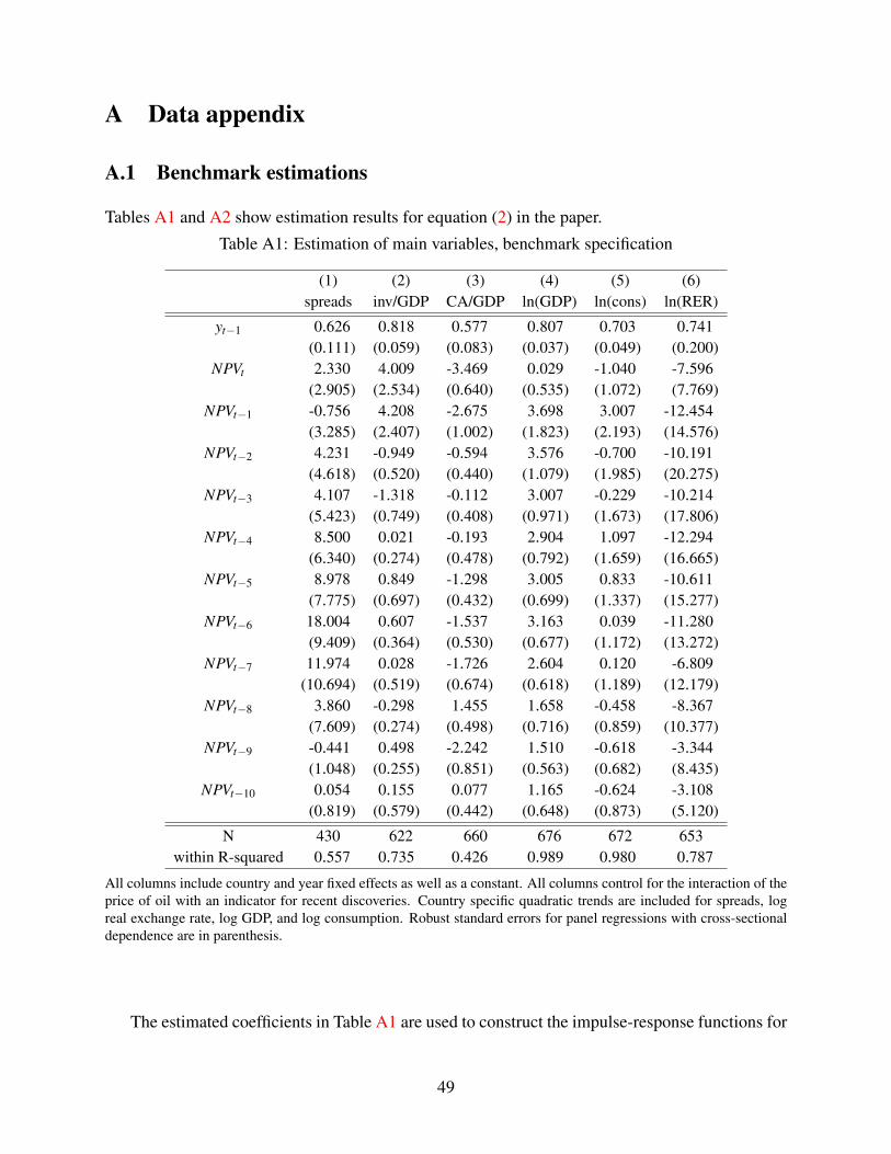
A Data appendix

A.1 Benchmark estimations

Tables A1 and A2 show estimation results for equation (2) in the paper.

Table A1: Estimation of main variables, benchmark specification

(1) (2) (3) (4) (5) (6)spreads inv/GDP CA/GDP ln(GDP) ln(cons) ln(RER)

yt−1 0.626 0.818 0.577 0.807 0.703 0.741(0.111) (0.059) (0.083) (0.037) (0.049) (0.200)

NPVt 2.330 4.009 -3.469 0.029 -1.040 -7.596(2.905) (2.534) (0.640) (0.535) (1.072) (7.769)

NPVt−1 -0.756 4.208 -2.675 3.698 3.007 -12.454(3.285) (2.407) (1.002) (1.823) (2.193) (14.576)

NPVt−2 4.231 -0.949 -0.594 3.576 -0.700 -10.191(4.618) (0.520) (0.440) (1.079) (1.985) (20.275)

NPVt−3 4.107 -1.318 -0.112 3.007 -0.229 -10.214(5.423) (0.749) (0.408) (0.971) (1.673) (17.806)

NPVt−4 8.500 0.021 -0.193 2.904 1.097 -12.294(6.340) (0.274) (0.478) (0.792) (1.659) (16.665)

NPVt−5 8.978 0.849 -1.298 3.005 0.833 -10.611(7.775) (0.697) (0.432) (0.699) (1.337) (15.277)

NPVt−6 18.004 0.607 -1.537 3.163 0.039 -11.280(9.409) (0.364) (0.530) (0.677) (1.172) (13.272)

NPVt−7 11.974 0.028 -1.726 2.604 0.120 -6.809(10.694) (0.519) (0.674) (0.618) (1.189) (12.179)

NPVt−8 3.860 -0.298 1.455 1.658 -0.458 -8.367(7.609) (0.274) (0.498) (0.716) (0.859) (10.377)

NPVt−9 -0.441 0.498 -2.242 1.510 -0.618 -3.344(1.048) (0.255) (0.851) (0.563) (0.682) (8.435)

NPVt−10 0.054 0.155 0.077 1.165 -0.624 -3.108(0.819) (0.579) (0.442) (0.648) (0.873) (5.120)

N 430 622 660 676 672 653within R-squared 0.557 0.735 0.426 0.989 0.980 0.787

All columns include country and year fixed effects as well as a constant. All columns control for the interaction of theprice of oil with an indicator for recent discoveries. Country specific quadratic trends are included for spreads, logreal exchange rate, log GDP, and log consumption. Robust standard errors for panel regressions with cross-sectionaldependence are in parenthesis.

The estimated coefficients in Table A1 are used to construct the impulse-response functions for

49

spreads, investment, the current account, GDP, consumption, and the real exchange rate.39 Table

A2 presents the point estimates of the coefficients ξs related to the interaction between the natural

logarithm of the price of oil poil,t and the indicator of an oil discovery in t− s for s = 1...10.

Table A2: Point estimates of interaction between price of oil and indicators of recent discoveries

(1) (2) (3) (4) (5) (6)spreads inv/GDP CA/GDP ln(GDP) ln(cons) ln(RER)

poil,tIdisc,i,t−1 -0.253 0.000 0.001 0.001 0.003 0.009(0.129) (0.001) (0.002) (0.002) (0.002) (0.008)

poil,tIdisc,i,t−2 -0.240 0.002 0.000 0.001 0.002 0.018(0.169) (0.001) (0.001) (0.001) (0.001) (0.011)

poil,tIdisc,i,t−3 -0.143 0.001 0.000 -0.001 0.000 0.008(0.250) (0.001) (0.001) (0.001) (0.001) (0.006)

poil,tIdisc,i,t−4 -0.376 -0.001 0.001 -0.002 0.002 0.010(0.207) (0.001) (0.001) (0.001) (0.001) (0.008)

poil,tIdisc,i,t−5 -0.142 0.001 0.001 -0.002 0.000 0.010(0.238) (0.001) (0.001) (0.001) (0.001) (0.006)

poil,tIdisc,i,t−6 0.245 -0.002 0.004 -0.002 -0.002 0.018(0.600) (0.001) (0.001) (0.002) (0.002) (0.011)

poil,tIdisc,i,t−7 0.043 -0.001 0.001 -0.001 0.000 0.008(0.190) (0.001) (0.001) (0.001) (0.001) (0.009)

poil,tIdisc,i,t−8 0.116 0.000 0.000 0.001 0.000 0.006(0.162) (0.001) (0.001) (0.001) (0.001) (0.012)

poil,tIdisc,i,t−9 0.120 0.000 0.001 0.001 0.000 0.004(0.157) (0.001) (0.001) (0.001) (0.001) (0.006)

poil,tIdisc,i,t−10 -0.430 0.001 -0.004 0.002 0.000 0.003(0.322) (0.001) (0.001) (0.001) (0.001) (0.004)

Robust standard errors for panel regressions with cross-sectional dependence are in parenthesis.

Note that the coefficients in column (1) are three orders of magnitude larger than those in

columns (2) through (5). Similarly, the coefficients in column (6) are also much larger than those

in columns (2) through (5). As discussed in the following section, this difference shows how the

inclusion of these control variables is relevant for the estimation of the effect of oil discoveries on

spreads and the real exchange rate but not for their effect on the rest of the variables.

Table A3 presents the estimation results for equation (2) in the paper that generate the impulse-

response functions in Figure (4). Column (1) presents the benchmark results, columns (2) and (3)

39Appendix A.3 shows the details about the estimation of the shares of investment in different sectors.

50

control for contemporaneous and up to ten lags of proved reserves, column (4) presents the results

using URR as a measure of the size of a discovery instead of their NPV.

Table A3: Regressions for spreads, main variables, benchmark and robustness

(1) (2) (3) (4)benchmark log(resi,t) log(resi,t−0...10) URRi,t

yt−1 0.626 0.623 0.574 0.575(0.111) (0.110) (0.096) (0.099)

NPVt 2.330 2.557 3.193 -0.025(2.905) (2.933) (3.559) (0.015)

NPVt−1 -0.756 -0.258 7.043 0.014(3.285) (3.602) (7.214) (0.015)

NPVt−2 4.231 5.600 16.737 0.040(4.618) (5.530 ) (12.051) (0.038)

NPVt−3 4.107 6.587 23.920 0.036(5.423) (7.319) (17.777) (0.024)

NPVt−4 8.500 9.470 26.651 0.052(6.340) (6.793) (17.117) (0.028)

NPVt−5 8.978 10.550 28.020 0.065(7.775) (8.767) (19.415) (0.045)

NPVt−6 18.004 19.260 20.425 0.168(9.409) (9.288) (6.009) (0.051)

NPVt−7 11.974 12.760 8.433 0.099(10.694) (11.126) (11.391) (0.062)

NPVt−8 3.860 4.176 -0.171 0.041(7.609) (8.100) (7.679) (0.040)

NPVt−9 -0.441 -0.563 -1.187 0.039(1.048) (1.045) (1.138) (0.034)

NPVt−10 0.054 0.026 -0.369 0.039(0.819) (0.824) (0.851) (0.031)

N 430 421 383 388within R-squared 0.556 0.561 0.600 0.611

All columns include country and year fixed effects as well as a constant and country specific quadratic trends. Allcolumns control for the interaction of the price of oil with an indicator for recent discoveries. Robust standard errorsfor panel regressions with cross-sectional dependence are in parenthesis.

Table (A4) below shows the estimated coefficients for proved reserves and their lags.

51

Table A4: Effect of reserves, point estimates

(1) (2) (3) (4)benchmark log(resi,t) log(resi,t−0...10) URRi,t

log(resi,t) 0.008 0.0251 0.023(0.015) (0.015) (0.012)

log(resi,t−1) 0.014 0.012(0.011) (0.009)

log(resi,t−2) 0.011 0.016(0.012) (0.012)

log(resi,t−3) 0.011 0.008(0.009) (0.007)

log(resi,t−4) 0.006 0.007(0.010) (0.010)

log(resi,t−5) 0.017 0.015(0.013) (0.012)

log(resi,t−6) 0.020 0.022(0.015) (0.015)

log(resi,t−7) -0.004 -0.004(0.018) (0.018)

log(resi,t−8) -0.017 -0.013(0.013) (0.013)

log(resi,t−9) -0.009 -0.010(0.006) (0.006)

log(resi,t−10) 0.001 0.002(0.006) (0.006)

Robust standard errors for panel regressions with cross-sectional dependence are in parenthesis.

A.2 Estimations without interaction control variables

Table A5 shows the estimation results for the following regression:

yi,t = ρyi,t−1 +10

∑s=0

ψsNPVi,t−s +αi +µt + εi,t

52

Table A5: Estimation of main variables, no interaction term

(1) (2) (3) (4) (5) (6)spreads inv/GDP CA/GDP ln(GDP) ln(cons) ln(RER)

yt−1 0.621 0.820 0.582 0.807 0.701 0.744(0.118) (0.060) (0.084) (0.036) (0.050) (0.197)

NPVt -1.491 3.937 -3.600 0.262 -1.078 -8.304(2.799) (2.479) (0.551) (0.620) (1.030) (7.972)

NPVt−1 -7.769 4.050 -2.082 4.394 0.996 -6.185(4.155) (2.110) (0.962) (1.780) (1.921) (10.852)

NPVt−2 -6.075 -0.776 -0.437 3.995 -1.465 -2.295(4.680) (0.410) (0.357) (1.066) (2.013) (15.110)

NPVt−3 -5.349 -1.176 0.135 3.183 -0.900 -3.170(4.502) (0.646) (0.311) (0.947) (1.733) (13.035)

NPVt−4 -3.212 -0.044 0.066 2.878 0.264 -5.286(5.341) (0.157) (0.374) (0.781) (1.597) (12.029)

NPVt−5 -1.386 1.022 -0.992 2.833 0.228 -3.368(6.427) (0.682) (0.267) (0.671) (1.382) (10.805)

NPVt−6 25.514 0.363 -0.756 2.574 -0.079 -4.525(13.036) (0.398) (0.390) (0.657) (1.219) (9.186)

NPVt−7 15.521 -0.243 -1.071 2.045 0.038 -0.994(7.267) (0.491) (0.569) (0.546) (1.223) (8.519)

NPVt−8 4.411 -0.498 2.107 1.330 -0.469 -3.264(6.384) (0.190) (0.434) (0.629) (0.913) (6.231)

NPVt−9 -0.975 0.245 -1.665 1.421 -0.616 0.151(1.131) (0.171) (0.763) (0.519) (0.743) (5.719)

NPVt−10 -0.457 0.237 -0.147 1.353 -0.652 -1.228(0.522) (0.634) (0.567) (0.617) (0.866) (3.235)

N 430 622 660 676 672 653within R-squared 0.545 0.731 0.414 0.989 0.980 0.786

All columns include country and year fixed effects as well as a constant. Country specific quadratic trends areincluded for spreads, log real exchange rate, log GDP, and log consumption. Robust standard errors for panelregressions with cross-sectional dependence are in parenthesis.

That is, equation 2 without controlling for the interaction between the price of oil and indicators

for recent discoveries. Comparing the results shown in Table A5 with those from Table A1 it is

clear that the interaction controls are of very little consequence for all regressions except for those

regarding spreads and the real exchange rate.

To illustrate this point even further, Figures A1, A2, and A3 show the impulse-response func-

tions constructed with the point estimates from Table A5.

53

Figure A1: Impact of giant oil discoveries on macroeconomic aggregates, no interaction term

Impulse response to an oil discovery with net present value equal to 4.5 percent of GDP, which is the median size ofdiscoveries in the sample. The dotted lines indicate 90 percent confidence intervals based on a Driscoll and Kraay(1998) estimation of standard errors, which yields standard error estimates that are robust to general forms of spatialand temporal clustering.

As is clear from comparing Figure A1 above with Figure 2 in the paper, the impulse-response

functions of investment, the current account, GDP, and consumption remain virtually unchanged

if we exclude the interaction controls. By comparing Figure A2 below with Figure 3 in the paper,

we can observe that the impact of oil discoveries on the dynamics of spreads is sensitive to the

inclusion of these interaction controls.

54

Figure A2: Impact of giant oil discoveries on spreads, no interaction term

Impulse response to an oil discovery with net present value equal to 4.5 percent of GDP, which is the median size ofdiscoveries in the sample. The dotted lines indicate 90 percent confidence intervals based on a Driscoll and Kraay(1998) estimation of standard errors, which yields standard error estimates that are robust to general forms of spatialand temporal clustering.

In both cases, with and without the interaction controls, the change in spreads peaks in the sev-

enth year after a discovery at around 5 percentage points. However, in the benchmark specification

spreads steadily increase in the years following a discovery, while in the specification that excludes

the interaction controls spreads first decrease during the first five years and then increase. These

differences are expected considering the sign of the coefficients reported in column (1) of Table

A2. These coefficients are negative for poil,tIdisc,i,t−s for s= 1...5, which implies that the coefficients

of NPVi,t−s for s = 1...5 are biased downward when the interaction terms are omitted.

55

Figure A3: Impact of giant oil discoveries on sectoral investment and the RER, no interaction term

Impulse response to an oil discovery with net present value equal to 4.5 percent of GDP, which is the median size ofdiscoveries in the sample. The dotted lines indicate 90 percent confidence intervals based on a Driscoll and Kraay(1998) estimation of standard errors, which yields standard error estimates that are robust to general forms of spatialand temporal clustering.

Figure A3 presents the impulse-response functions of the real exchange rate and the shares of

total investment that go into manufacturing, commodities, and non-traded sectors for the estima-

tions that do not consider the interaction controls. As is clear by comparing Figure A3 above with

Figure 4 in the paper, only the response of the real exchange rate is affected by the omission.40

Given the sign of the coefficients reported in column (6) of Table A2, the coefficients of NPVi,t−s

for s = 1...10 are biased upward when the interaction terms are omitted.

A.3 The effect of oil discoveries on investment shares by sector

This Section provides details on the estimation of the effect of oil discoveries on the share of total

investment in manufactures, commodities, and non-traded sectors. These estimates consider 4740Note how the coefficients in column (6) of Table A2 are much larger than the coefficients reported in Table A8.

56

countries for which sectoral investment data for the period 1993–2012 are available.41

The data of investment by sector are from the National Accounts Official Country Data col-

lected by the United Nations following the International Standard Industrial Clasification, Revision

3 (ISIC Rev. 3). It considers investment per country for 11 sub-items. Table A6 summarizes the

sub-items and how I classify them into non-traded, manufacturing, and commodities.

Table A6: Industry classification

sub-item clasification

Agriculture, hunting, forestry; fishing (A+B) commoditiesMining and quarrying (C) commodities

Manufacturing (D) manufacturingElectricity, gas and water supply (E) non-traded

Construction (F) non-tradedWholesale retail; hotels and restaurants (G+H) non-traded

Transport, storage and communications (I) non-tradedFinancial intermediation; real estate (J+K) non-traded

Public administration; compulsory social security (L) non-tradedEducation; health and social work; other (M+N+O) non-traded

Private households with employed persons (P) non-traded

Tables A7 and A8 show the estimation results for equation (2) in the paper. The estimated

coefficients in Table A7 are used to construct the impulse-response functions for the shares of total

investment that go into manufacturing, commodities, and non-traded sectors reported in Figure 4

in the paper.

41These countries are Armenia, Australia, Austria, Azerbaijan, Belarus, Belgium, Botswana, Canada, Cyprus, Den-mark, Estonia, Finland, France, Germany, Greece, Hungary, Iceland, Ireland, Italy, Kuwait, Latvia, Lithuania, Luxem-bourg, Malta, Mauritius, Mexico, Namibia, Netherlands, New Zealand, Norway, Oman, Pakistan, Poland, Portugal,Qatar, Saudi Arabia, Slovenia, South Africa, Spain, Sweden, Syrian Arab Republic, Tunisia, Ukraine, United ArabEmirates, United Kingdom, United States, and Uruguay.

57

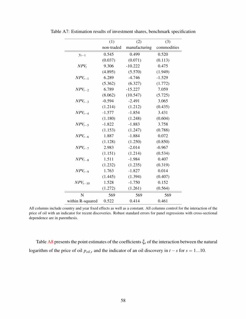
Table A7: Estimation results of investment shares, benchmark specification

(1) (2) (3)non-traded manufacturing commodities

yt−1 0.545 0.499 0.520(0.037) (0.071) (0.113)

NPVt 9.306 -10.222 0.475(4.895) (5.570) (1.949)

NPVt−1 6.289 -4.746 -1.529(5.362) (6.327) (1.772)

NPVt−2 6.789 -15.227 7.059(8.062) (10.547) (5.725)

NPVt−3 -0.594 -2.491 3.065(1.214) (1.212) (0.435)

NPVt−4 -1.577 -1.854 3.431(1.180) (1.248) (0.604)

NPVt−5 -1.822 -1.883 3.758(1.153) (1.247) (0.788)

NPVt−6 1.887 -1.884 0.072(1.128) (1.250) (0.850)

NPVt−7 2.983 -2.014 -0.967(1.151) (1.214) (0.534)

NPVt−8 1.511 -1.984 0.407(1.232) (1.235) (0.319)

NPVt−9 1.763 -1.827 0.014(1.445) (1.394) (0.407)

NPVt−10 1.528 -1.750 0.152(1.272) (1.261) (0.564)

N 569 569 569within R-squared 0.522 0.414 0.461

All columns include country and year fixed effects as well as a constant. All columns control for the interaction of theprice of oil with an indicator for recent discoveries. Robust standard errors for panel regressions with cross-sectionaldependence are in parenthesis.

Table A8 presents the point estimates of the coefficients ξs of the interaction between the natural

logarithm of the price of oil poil,t and the indicator of an oil discovery in t− s for s = 1...10.

58

Table A8: Point estimates of interaction between price of oil and indicators of recent discoveries

(1) (2) (3)non-traded manufacturing commodities

poil,tIdisc,i,t−1 -0.002 0.002 0.000(0.003) (0.002) (0.002)

poil,tIdisc,i,t−2 -0.001 0.001 0.000(0.001) (0.002) (0.002)

poil,tIdisc,i,t−3 -0.002 0.003 -0.001(0.003) (0.001) (0.003)

poil,tIdisc,i,t−4 0.002 0.001 -0.003(0.002) (0.001) (0.001)

poil,tIdisc,i,t−5 0.002 0.000 -0.001(0.002) (0.002) (0.002)

poil,tIdisc,i,t−6 -0.001 0.000 0.001(0.001) (0.001) (0.001)

poil,tIdisc,i,t−7 -0.003 0.003 0.001(0.002) (0.004) (0.002)

poil,tIdisc,i,t−8 -0.001 0.000 0.002(0.002) (0.002) (0.001)

poil,tIdisc,i,t−9 0.001 -0.005 0.004(0.002) (0.001) (0.001)

poil,tIdisc,i,t−10 -0.001 0.001 0.000(0.001) (0.001) (0.002)

Robust standard errors for panel regressions with cross-sectional dependence are in parenthesis.

Finally, Table A9 shows the estimation results for the following regression:

yi,t = ρyi,t−1 +10

∑s=0

ψsNPVi,t−s +αi +µt + εi,t

that is the same as equation (2) but without controlling for the interaction between the price of oil

and indicators for recent discoveries.

59

Table A9: Estimation results of investment shares, no interaction term

(1) (2) (3)non-traded manufacturing commodities

yt−1 0.551 0.496 0.533(0.036) (0.069) (0.112)

NPVt 8.047 -9.735 1.098(4.220) (5.216) (1.844)

NPVt−1 4.418 -3.351 -1.191(4.909) (5.912) (2.252)

NPVt−2 3.654 -13.469 8.607(7.419) (7.988) (3.840)

NPVt−3 -0.958 -2.228 3.184(1.087) (1.254) (0.483)

NPVt−4 -1.598 -1.734 3.280(1.052) (1.233) (0.638)

NPVt−5 -1.868 -1.909 3.765(1.024) (1.234) (0.763)

NPVt−6 1.614 -1.871 0.264(1.009) (1.247) (0.874)

NPVt−7 2.437 -1.734 -0.744(1.057) (1.302) (0.618)

NPVt−8 1.175 -2.000 0.757(1.055) (1.166) (0.326)

NPVt−9 1.683 -2.453 0.720(1.251) (1.298) (0.367)

NPVt−10 1.268 -1.705 0.318(1.178) (1.396) (0.526)

N 569 569 569within R-squared 0.514 0.398 0.449

All regressions include country and year fixed effects as well as a constant. Robust standard errors for panelregressions with cross-sectional dependence are in parenthesis.

60

B Computation

B.1 Simplifying the recursive problems

The value of the government in repayment, defined in Subsection 3.2, is:

V P (s,k,koil,b) = max{k′,k′oil ,b

′,C,K,X}

{u(c)+βGE

[V(s′,k′,k′oil,b

′)]}subject to the following constraints:

c+ ik + ikoil = Y −Ψ(k′,k)−Ψ

(k′oil,koil

)k′ = (1−δ )k+ ik

k′oil = (1−δ )koil + ikoil

Y = fY (cN ,cM,coil)

cN = z f N (kN)

cM + xM = z f M (kM)

kN + kM = k

coil + xoil = f oil (koil,n)

xM + poilxoil = γb−q(s,k′,k′oil,b

′)[b′− (1− γ)b]

where C = {c,cN ,cM,coil} ,K = {kN ,kM}, X = {xM,xoil} are all the static allocations,

fY (cN ,cM,coil) = A[

ω

1η

N (cN,t)η−1

η +ω

1η

M (cM,t)η−1

η +ω

1η

oil

(coil,t

)η−1η

] η

η−1

, f N (k) = kαN , f M (k) =

kαM , and f oil (koil,n) =[

α

1ϕ

oil (koil)ϕ−1

ϕ +ζ1ϕ (n)

ϕ−1ϕ

] ϕ

ϕ−1

. The above set of constraints can be sim-

plified by defining the production possibility frontier for the final good as:

FP (s,k,koil,T ) = maxcN ,cM ,coil ,λ

fY (cN ,cM,coil)

s.t. cN = z f N ((1−λ )k)

cM + poilcoil +T = z f M (λk)+ poil f oil (koil,n)

61

where T = γb− q(s,k′,k′oil,b

′) [b′− (1− γ)b] are net debt payments to the rest of the world and

λ ∈ [0,1] is the share of capital allocated in the manufacturing sector. Given the state and a choice

for(k′,k′oil,b

′), the first-order conditions of the maximization problem in the right-hand-side of FP

pin down the efficient static allocations for the current period:

cN = z f N ((1−λ )k) (15)

cM =ωM

ωoil(poil)

η coil (16)

poilcoil =ωoil (poil)

1−η

ωM +ωoil (poil)1−η

[z f M (λk)+ poil f oil (z,koil,n)−T

](17)(

αM

αN

(1−λ )1−αN

λ 1−αM(k)αM−αN

)η

z f N ((1−λ )k) =ωN

ωM +ωoil (poil)1−η

[z f M (λk)+ poil f oil (z,koil,n)−T

](18)

The value function of the government in repayment can be rewritten as:

V P (s,k,koil,b) = maxc,k′,k′oil ,b

′

{u(c)+βEs′|sV

(s′,k′,k′oil,b

′)}s.t. c+ i+ ioil = FP (s,k,koil,b,T )−Ψ

(k′,k)−Ψ

(k′oil,koil

)k′ = i+(1−δ )k

k′oil = ioil +(1−δ )koil

T = γb−q(s,k′,k′oil,b

′)[b′− (1− γ)b]

Doing the same for the value in default we get:

V D (s,k,koil) = maxc,k′,k′oil

{u(c)+βEs′|s

[θV(s′,k′,k′oil,0

)+(1−θ)V D (s′,k′,k′oil

)]}s.t. c+ i+ ioil = FD (s,k,koil)−Ψ

(k′,k)−Ψ

(k′oil,koil

)k′ = i+(1−δ )k

k′oil = ioil +(1−δ )koil

62

where

FD (s,k,koil) = maxcN ,cM ,coil ,kN ,kM

fY (cN ,cM,coil)

s.t. cN = zd (z) f N (kN)

cM + poilcoil = zd (z) f M (kM)+ poil f oil (koil,n)

B.2 Pre-computing output

Evaluating FP and FD involves finding the root of equation (18), which can become computation-

ally burdensome within a value function iteration algorithm.

Note that FD does not depend on the value functions or the price of the debt q, which

change as the algorithm converges, so it can be pre-calculated exactly for all possible states

(s,k,koil) and stored in memory. This pre-calculation, however, cannot be done for FP, since

the static allocations depend also on the current borrowing and investment choices through

T = γb−q(s,k′,k′oil,b

′) [b′− (1− γ)b]. In order to achieve similar gains, I pre-calculate FP for all

possible states (s,k,koil,b) and for a grid of plausible trade balances T .

In order to evaluate FP at a given state and policy choice, I compute T = γb −

q(s,k′,k′oil,b

′) [b′− (1− γ)b] and approximate FP by linearly interpolating over the pre-calculated

values for T (for the chosen value of η , F (s,k,koil, ·) is close to linear). This is much faster than

finding the root of equation (18) inside each iteration on the Bellman equations and less compu-

tationally demanding than storing in memory all the values of FP for all possible combinations of(s,k,koil,b,k′,k′oil,b

′).

63

Acknowledgments: I am grateful to Manuel Amador and Tim Kehoe for their mentoring and

guidance. For comments and discussions I thank Ana María Aguilar, Cristina Arellano, David

Argente, Marco Bassetto, Anmol Bhandari, Javier Bianchi, David Bradley, Marcos Dinerstein,

Doireann Fitzgerald, Stelios Fourakis, Carlo Galli, Salomón García, Eugenia González-Aguado,

Pierre-Olivier Gourinchas, Loukas Karabarbounis, Tobey Kass, Todd Keister, Juan Pablo Nicolini,

Fausto Patiño, Fabrizio Perri, Agustín Sámano, César Sosa-Padilla, Venky Venkateswaran, and

Steve Wu. I also thank seminar participants at the Federal Reserve Bank of Minneapolis, the Min-

nesota Trade Workshop, the Minnesota-Wisconsin International/Macro Workshop, Rutgers Uni-

versity, the 2019 ITAM alumni conference, the 2020 SED meeting, the 2020 Canadian Economics

Association virtual meeting, and the EEA 2020 virtual meeting. I acknowledge generous support

from the Hutcheson-Lilly dissertation fellowship. All errors are my own.

References

Aguiar, Mark and Manuel Amador. 2011. “Growth in the shadow of expropriation.” Quarterly

Journal of Economics 126:651–697. 13, 19

———. 2014. “Sovereign Debt.” In Handbook of International Economics, vol. 4. 647–687. 21

Aguiar, Mark, Manuel Amador, and Stelios Fourakis. 2020. “On the Welfare Losses from External

Sovereign Borrowing.” IMF Economic Review 68 (1):163–194. 46

Aguiar, Mark, Satyajit Chatterjee, Harold L. Cole, and Zachary Stangebye. 2016. “Quantitative

Models of Sovereign Debt Crises.” In Handbook of Macroeconomics. 21, 24

Aguiar, Mark and Gita Gopinath. 2006. “Defaultable Debt, Interest Rates and the Current Ac-

count.” Journal of International Economics 69 (1):64–83. 5, 27

———. 2007. “Emerging Market Business Cycles: The Cycle Is the Trend.” Journal of Political

Economy 115 (1):71–102. 24

Alberola, Enrique and Gianluca Benigno. 2017. “Revisiting the commodity curse: A financial

perspective.” Journal of International Economics 108:87–106. 3

64

Amador, Manuel. 2012. “Sovereign Debt and The Tragedy of the Commons.” Working Paper. 19

Arellano, C. and Ananth Ramanarayanan. 2012. “Default and the Maturity Sturcture in Sovereign

Bonds.” Journal of Political Economy 120 (2):187–232. 20

Arellano, Cristina. 2008. “Default Risk and Income Fluctuations in Emerging Economies.” Amer-

ican Economic Review 98 (3):690–712. 5, 20

Arellano, Cristina, Yan Bai, and Gabriel Mihalache. 2018. “Default risk, sectoral reallocation, and

persistent recessions.” Journal of International Economics 112:182–199. 5

Arellano, Manuel and Stephen Bond. 1991. “Some Tests of Specification for Panel Dada: Monte

Carlo Evidence and an Application to Employment Equations.” The Review of Economic Studies

58 (2):277–297. 11

Arezki, Rabah, Valerie A. Ramey, and Liugang Sheng. 2017. “News Shocks in Open Economies:

Evidence From Giant Oil Discoveries.” Quarterly Journal of Economics :103–155. 1, 2, 3, 4, 7,

8, 10, 11, 12, 13, 14, 15, 16, 19, 24, 26, 27, 32

Ayres, Joao, Constantino Hevia, and Juan Pablo Nicolini. 2019. “Real Exchange Rates and Primary

Commodity Prices.” Federal Reserve Bank of Minneapolis Staff Report (584). 6

Beaudry, Paul and Franck Portier. 2014. “News-Driven Business Cycles: Insights and Callenges.”

Journal of Economic Literature 52 (4):993–1074. 4

Bianchi, Javier. 2011. “Overborrowing and Systemic Externalities in the Buisness cycle.” Ameri-

can Economic Review 101:3400–3426. 24

Bianchi, Javier, Juan Carlos Hatchondo, and Leonardo Martinez. 2018. “International Reserves

and Rollover Risk.” American Economic Review 108 (9):2629–2670. 24

Bornstein, Gideon, Per Krusell, and Sergio Rebelo. 2019. “Lags, Costs, and Shocks: Shocks: An

Equilibrium Model of the Oil Industry.” 19

Broner, Fernando A., Guido Lorenzoni, and Sergio L. Schmukler. 2013. “Why Do Emerging

Economies Borrow Short Term?” Journal of the European Economic Association 11 (1):67–

100. 27

65

Chatterjee, Satyajit and Burcu Eyigungor. 2012. “Maturity, Indebtedness, and Default Risk.”

American Economic Review 102 (6):2674–2699. 5, 20

Cole, Harold L. and Timothy J. Kehoe. 2000. “Self-Fulfilling Debt Crises.” Review of Economic

Studies 67:91–116. 21

Cuadra, Gabriel and Horacio Sapriza. 2008. “Sovereign Default, Interest Rates and Political Un-

certainty in Emerging Markets.” Journal of International Economics 76 (1):78–88. 19

Division, United Nations Statistics. 2017. National Accounts Official Country Data. United Na-

tions, New York, NY, 2017 ed. 12

Driscoll, John C. and Aart C. Kraay. 1998. “Consistent Covariance Matrix Estimation with Spa-

tially Dependent Panel Data.” Review of Economics and Statistics 80:549–560. 13, 14, 16, 54,

55, 56

Eaton, Jonathan and Mark Gersovitz. 1981. “Debt with Potential Repudiation: Theoretical and

Empirical Analysis.” The Review of Economic Studies 48 (2):289–309. 5, 17, 21

Esquivel, Carlos, Thimothy J. Kehoe, and Juan Pablo Nicolini. 2020. “Lessons from the Monetary

and Fiscal History of Latin America.” 33

Fund, International Monetary. 2013. World Economic Outlook (WEO). International Monetary

Fund, Washington, DC, 2013 ed. 12

Galli, Carlo. 2019. “Self-Fulfilling Debt Crises, Fiscal Policy and Investment.” Working Paper. 22

Gordon, Grey and Pablo A. Guerron-Quintana. 2018. “Dynamics of investment, debt, and Default.”

Review of Economic Dynamics 28:71–95. 5, 18, 36, 38

Group, World Bank. 2013. World Development Indicators (WDI). World Bank Group, Washington,

DC, 2013 ed. 12, 28

Gunn, Christopher M. and Alok Johri. 2013. “Fear of Sovereign Default, Banks, and Expectations-

driven Business Cycles.” Tech. rep., Carleton Economic Papers (CEP). 5

66

Hamann, Franza, Enrique G. Mendoza, and Paulina Restrepo-Echavarria. 2020. “Resource Curse

or Blessing? Sovereign Risk in Resource-Rich Emerging Economies:.” Unpublished manuscript

presented at the 2020 Atlanta Workshop on International Economics. 5, 6, 9, 10, 15, 19

Hatchondo, Juan Carlos and Leonardo Martinez. 2009. “Long-Duration Bonds and Sovereign

Defaults.” Journal of International Economics 79 (1):117–125. 5, 20

Hatchondo, Juan Carlos, Leonardo Martinez, and Horacio Sapriza. 2010. “Quantitative proper-

ties of sovereign default models: Solution methods matter.” Review of Economic Dynamics

13 (4):919–933. 23

Hatchondo, Juan Carlos, Leonardo Martinez, and Cesar Sosa-Padilla. 2016. “Debt Dilution and

Sovereign Default Risk.” Journal of Political Economy 124 (5):1383–1422. 39

Hevia, Constantino, Pablo Andres Neumeyer, and Juan Pablo Nicolini. 2013. “Optimal Monetary

and Fiscal Policy in a New Keynesian Model with a Dutch Disease: The Case of Complete

Markets.” Universidad di Tella Working Paper . 3

Hevia, Constantino and Juan Pablo Nicolini. 2015. “Monetary Policy and Dutch Disease: The

Case of Price and Wage Rigidity.” Federal Reserve Bank of Minneapolis Working Paper (726).

6

Horn, Myron K. 2014. “Giant Oil and Gas Fields of the World.”

Https://edx.netl.doe.gov/dataset/aapg-datapages-giant-oil-and-gas-fields-of-the-world. 1,

8

Jacks, David S., Kevin H. O’Rourke, and Jeffrey G. Williamson. 2011. “Commodity Price Volatil-

ity and World Market Integration Since 1700.” Review of Economics and Statistics 93 (3):800–

813. 2

Jaimovich, Nir and Sergio Rebelo. 2008. “News and Business Cycles in Open Economies.” Journal

of Money, Credit and Banking 40 (8):1699–1711. 4

Lei, Yu-Hsiang and Guy Michaels. 2014. “Do giant oilfield discoveries fuel international armed

conflicts?” Journal of Development Economics 110:139–157. 3

67

Mendoza, Enrique. 1991. “Real Buisness Cycles in a Small Open Economy.” American Economic

Review 81 (4):797–818. 18

Mendoza, Enrique G. 1995. “The Terms of Trade, the Real Exchange Rate, and Economic Fluctu-

ations.” International Economic Review 36 (1):101–137. 24, 26

———. 2005. “Real Exchange Rate Volatility and the Price of Nontradable Goods in Economies

Prone to Sudden Stops.” Economia: Journal of the Latin American and Caribbean Economic

Association 6 (1):103–135. 24

Mendoza, Enrique G. and Vivian Z. Yue. 2012. “A General Equilibrium Model of Sovereign

Default and Buisness Cycles.” Quarterly Journal of Economics 127:889–946. 20

Nelder, John A. and R. Mead. 1965. “A Simplex Method for Function Minimization.” The Com-

puter Journal 7 (4):308–313. 23

Nickell, Stephen. 1981. “Biases in Dynamic Models with Fixed Effects.” Econometrica

49 (6):1417–1426. 11

Obstfeld, Maurice and Kenneth Rogoff. 1995. “The Intertemporal Approach to the Current Ac-

count.” In Handbook of International Economics, vol. 3, edited by Gene M. Grossman and

Kenneth Rogoff. Elsevier, 1731–1799. 7

Stockman, Alan C. and Linda L. Tesar. 1995. “Tastes and Technology in a Two-Country Model

of the Buisness Cycle: Explaining International Comovements.” American Economic Review

85 (1):168–185. 24

Tauchen, George. 1986. “Finite state markov-chain approximations to univariate and vector au-

toregressions.” Economic Letters 20 (2):177–181. 25

Tomz, Michael and Mark L. J. Wright. 2007. “Do Countries Default in "Bad Times"?” Journal of

the European Economic Association 5 (2-3):352–360. 1, 29

Tornell, Aaron and Philip R. Lane. 1999. “The Voracity Effect.” American Economic Review

89 (1):22–46. 32

68