MICROSCALE FLUCTUATIONS IN THE SOLAR WIND An invited review

Aaron Barnes

Theoretical constraints on the interpretation of fluctuations (either propagating or stationary) in the interplanetary medium are reviewed, with emphasis on the important differences between the properties of hydromagnetic waves (and stationary structures) in collisionless and in collision-dominated plasmas, and on the possible roles of Landau damping and nonlinear effects in determining the interplanetary fluctuation spectrum. Hypotheses about the origins of the fluctuations and their influence on the large-scale properties of the solar wind are reviewed.

ABSTRACT

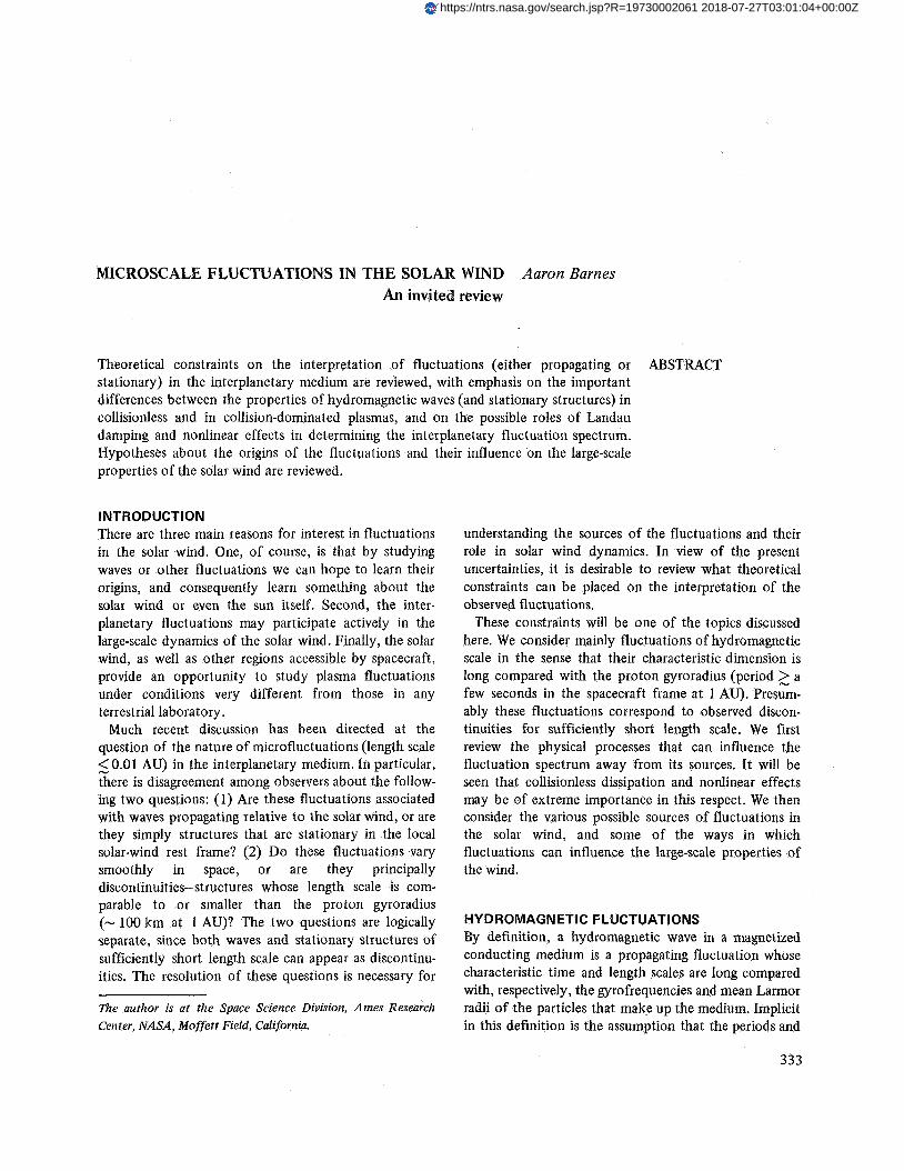
INTRODUCTION There are three main reasons for interest in fluctuations in the solar wind. One, of course, is that by studying waves or other fluctuations we can hope to learn their origins, and consequently learn something about the solar wind or even the sun itself. Second, the inter- planetary fluctuations may participate actively in the large-scale dynamics of the solar wind. Finally, the solar wind, as well as other regions accessible by spacecraft, provide an opportunity to study plasma fluctuations under conditions very different from those in any terrestrial laboratory.

Much recent discussion has been directed at the question of the nature of microfluctuations (length scale 5 0.01 AU) in the interplanetary medium, In particular, there is disagreement among observers about the follow- ing two questions: (1) Are these fluctuations associated with waves propagating relative to the solar wind, or are they simply structures that are stationary in the local solar-wind rest frame? (2) Do these fluctuations vary smoothly in space, or are they principally discontinuities-structures whose length scale is com- parable to or smaller than the proton gyroradius (- 100 km at 1 AU)? The two questions are logically separate, since both waves and stationary structures of sufficiently short length scale can appear as discontinu- ities. The resolution of these questions is necessary for

The author is at the Space Science Division, Ames Research Center, NASA, Moffett Field, California.

understanding the sources of the fluctuations and their role in solar wind dynamics. In view of the present uncertainties, it is desirable to review what theoretical constraints can be placed on the interpretation of the observed fluctuations.

These constraints will be one of the topics discussed here. We consider mainly fluctuations of hydromagnetic scale in the sense that their characteristic dimension is long compared with the proton gyroradius (period 2 a few seconds in the spacecraft frame at 1 AU). Presum- ably these fluctuations correspond to observed discon- tinuities for sufficiently short length scale. We first review the physical processes that can influence the fluctuation spectrum away from its sources. I t will be seen that collisionless dissipation and nonlinear effects may be of extreme importance in this respect. We then consider the various possible sources of fluctuations in the solar wind, and some of the ways in which fluctuations can influence the large-scale properties of the wind.

HYDROMAGNETIC FLUCTUATIONS By definition, a hydromagnetic wave in a magnetized conducting medium is a propagating fluctuation whose characteristic time and length scales are long compared with, respectively, the gyrofrequencies and mean Larmor radii of the particles that make up the medium. Implicit in this definition is the assumption that the periods and

333

https://ntrs.nasa.gov/search.jsp?R=19730002061 2018-07-27T03:01:04+00:00Z

wavelengths of the fluctuations are short in comparison with the time and length scales for significant changes in the average properties of the medium. Just as large-scale motions in an ordinary gas are associated with sound waves, the large-scale motions in a magnetized con- ducting fluid are associated with hydromagnetic waves. We can expect such processes as the violent stirring in the solar photosphere, chromosphere and corona, or the collision between fast and slow solar-wind streams, among others, to be associated with the generation of hydromagnetic waves.

The simplest approach to the theory of hydromagnetic waves is through the equations of magnetohydro- dynamics [Kantrowitz and Petschek, 1966; Landau and Lifshitz, 19601. Although these equations (which describe the behavior of collision-dominated ionized gases) cannot properly be used to describe hydromag- netic waves in the solar-wind plasma, where collisionless effects are important, they do provide a useful set of concepts and definitions that help to order the complex- ities of the collisionless theory. Hence, it is useful to review briefly the main results of the MHD theory of hydromagnetic waves.

First, consider the case in which the amplitudes of the fluctuations are small enough that the MHD equations can be linearized with the usual assumptions that the electrical conductivity of the medium is infinite and that the fluctuations are thermally adiabatic. The self-consis- tent solutions of the MHD equations admit three true wave modes (the Alfvkn mode, and the fast and slow magnetoacoustic modes) and two classes of stationary fluctuations (the so-called entropy wave and the tangen- tial pressure balance). The AlfvCn wave is transverse and involves no compression of the fluid or magnetic field. The fast and slow magnetoacoustic waves generally involve compressions of both the fluid and magnetic field; in the limit of strong magnetic field the fast mode propagates with the AlfvCn speed for all directions of propagation, and in the limit of weak magnetic field the fast mode becomes a sound wave. The entropy wave is a static structure involving variation of fluid density and temperature, but not of pressure, magnetic field or velocity. The tangential pressure balance can occur only for variations that are transverse to the magnetic field and for which the total pressure (fluid plus magnetic) does not fluctuate.

When finite-amplitude effects are significant, the fast and slow magnetoacoustic waves behave like sound waves in the sense that they can steepen and form shocks. On the other hand, the AlfvCn wave is more like an elliptically polarized electromagnetic wave. Even when its amplitude is large, it retains many of its

small-amplitude features: It is noncompressive, and the relation between velocity and magnetic-fieid fluctuations is the same as in the linearized theory. The finite-ampli- tude AlfvCn wave may have any polarization consistent with constant magnitude of the fluctuation field (hence, for example, linear polarization is forbidden). It does not steepen to form shocks in a homogeneous medium.

There are other important nonlinear effects. Nonlinear wave decay and mode coupling may occur, even for the AlfvCn wave. In the case of the magnetoacoustic modes, there are shock waves. In the limit of zero wavelength, the Alfvbn wave is known as the rotational disconti- nuity, the entropy wave as the contact discontinuity, and the tangential pressure balance as the tangential discontinuity. Being stationary structures, the entropy wave and tangential pressure balance are not subject to steepening effects, but may be unstable under some circumstances.

COLLISIONLESS HYDROMAGNETIC WAVES The preceding magnetohydrodynamic picture must be modified in situations in which collisionless effects are important-when the wave frequencies are large com- pared with the Coulomb collision frequencies of the plasma particles. In this sense the protons, and to a large extent the electrons, are collisionless with respect to most interesting hydromagnetic waves throughout the solar wind. For example, at 1 AU protons are collision- less with respect to waves of period shorter than about 12 hr (as measured in the spacecraft frame), and electrons are collisionless with respect to periods shorter than about 3 hr. At heliocentric distance r = 2R,, protons and electrons are collisionless with respect to wave periods shorter than about 10 min, and 20 sec, respectively. Hence, to understand hydromagnetic waves in the solar wind, a collisionless theory is required.

The wave mode that is least changed by collisionless effects is the AlfvCn wave [Stepanov, 1958; Barnes, 1966; Tajiri, 19671. In the limit of small amplitude, this wave is transverse, and its energy flux (as viewed in the rest frame of the plasma) is always parallel to the mean magnetic field direction. Its phase velocity follows from the dispersion relation

Here w is the circular frequency and kll is the compo- nent of the wave vector parallel to the magnetic field, B is the magnetic field strength, p is the mass density,

334

P ( I I , I ) are the components of total fluid pressure transverse and parallel to the magnetic field direction, and CA is the usual AlfvCn speed. The collisionless character of the plasma appears only through the pressure anisotropy. As is well known, this mode becomes nonresonantly unstable if PiI/Pl is large enough that the right-hand side of the preceding expression is negative. Counterstreaming of different ion species along the magnetic field lines can produce similar effects. If a significant high-energy tail of the proton velocity distri- bution is present, the AlfvCn mode can be further modified by wave-particle cyclotron resonance, with consequent damping or growth of the wave.

As in the MHD theory, the collisionless AlfvCn mode is not greatly modified by finite-amplitude effects [Barnes and Suffolk, 19711. It is still noncompressive, the usual relation between velocity and magnetic-field fluctuations still holds, and the magnetic field associated with the wave is of constant magnitude. Its polarization is indeterminate, except for the requirement that the magnitude of the fluctuating field be constant, which of course rules out plane polarization. These conclusions are valid for AlfvCn waves of arbitrary amplitude. It may also be shown that these statements are valid even when relativistic effects are important (although the dispersion relation is somewhat modified by relativity). In parti- cular, the criterion for the firehose instability is un- changed by relativity and finite-amplitude effects.

However, just as in the MHD case, the fact that large-amplitude AlfvCn waves are very much like their small-amplitude counterparts does not mean that the large-amplitude waves may be superposed as in the linearized theory. Two large-amplitude AlfvCn waves interact in a nonlinear manner, generating turbulence in other wave modes. In fact, a large-amplitude AlfvCn wave may be unstable against decay, an effect that may be of importance for understanding solar-wind turbu- lence.

Although the properties of the AlfvCn mode in a stable plasma do not depend much on whether the plasma is collisionless or collision-dominated, the collisionless magnetoacoustic modes differ radically from their MHD counterparts. This difference is due to the strong resonant wave-particle energy exchange that can occur in the collisionless case, usually resulting in strong collision- less damping of magnetoacoustic modes [Stepanov, 1958; Barnes, 1966; Tajiri, 19671. The resonant inter- action of importance here involves particles whose motion along the magnetic field is such that they see the wave frequency Doppler shifted to zero-that is, V I I = w/kll, where vi1 is the component of particle velocity along the magnetic field, w is the circular

frequency of the wave, and kll is the coniponent of the wave vector along the magnetic field. This kind of resonance is usually called Landau resonance, as opposed to cyclotron resonance, which occurs when the resonant particles see the wave frequency Doppler shifted to an integral multiple of their gyrofrequency. Cyclotron resonance is normally negligible for hydromagnetic waves, but Landau resonance is not.

Physically, the resonant acceleration is due to the fact that in a collisionless plasma a gradient in magnitude of the magnetic field accelerates the guiding center of a particle along the magnetic field [Barnes, 19671. This acceleration tends to produce a small charge separation and an associated electric field parallel to the magnetic field; this electric field, which also contributes to the resonant energy exchange, is proportional to the gradi- ent in the magnetic field magnitude, and vanishes if this gradient vanishes. Hence the resonant energy exchange depends on the presence of fluctuations in magnetic field magnitude in the wave. Therefore, this interaction will occur for magnetoacoustic waves, but not for AlfvCn waves, because the AlfvCn mode is associated with fluctuations in direction, but not magnitude, of the magnetic field.

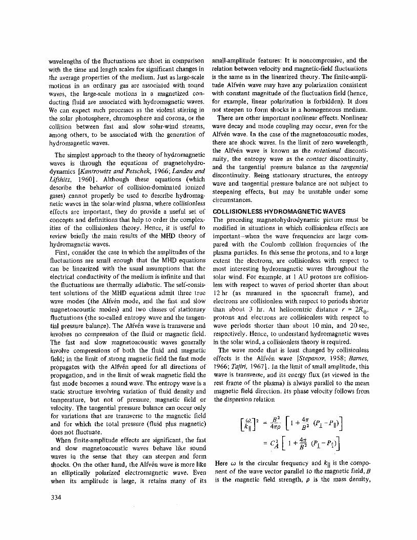
Consider a stable collisionless hydrogen plasma whose components have bi-maxwellian velocity distributions. In such a plasma the resonant acceleration always produces damping of the waves. An example of this damping is shown in figure 1. The theoretical damping rate per unit frequency 1 Zm(w)/Re(o) 1 is plotted as a function of propagation direction, for small-amplitude magnetoacoustic waves in plasmas whose proton and electron temperatures are equal and isotropic. The resonant heating and consequent damping are maxima for directions of propagation such that w/kll is roughly

,--- ---- P ' 5 } SLOW MODE p = I /

Figure 1. for magnetoacoustic waves in two isotropic plasmas.

Damping rate versus propagation direction

335

equal to the proton and electron thermal speeds. The resonant heating, especially for the ions, is sensitive to average plasma conditions, because the heating rate is largely determined by the number of particles available for resonance. For maxwellian proton distributions, the proton heating rate per unit wave energy for the least-damped mode is roughly proportional to exp - [ l/Ppcos2 e ] where p p = 87rn KT / B 2 , np and Tp are the proton number density and temperature, B is the magnetic field strength, and K is Boltzmann’s constant. Thus the damping depends strongly on op, the ratio of the proton pressure to magnetic pressure. If oP 2 1, the damping is strong, but as oP -+ 0, the damping becomes exponentially weak. This dependence is illustrated below:

P P

Characteristic time of strongest

0, proton damping

1 - 2 wave periods 0.5 - 10 wave periods 0.2 - 200 wave periods

-

If one takes typical solar-wind parameters at 1 AU as number density n = 7 protons ~ m - ~ , proton temperature Tp = 4 X 104”K, and magnetic field B = 5 X lo-’ gauss, the resulting P p =0.4. The observational study of Burhga et al. [1969] indicates that this parameter can range from less than 0.1 to more than 5.0. If we suppose that P p -0.3 to 0.5 for most of the distance between the sun and the orbit of earth, compressive hydromagnetic waves will be damped out in 10 to 100 wavelengths. Thus jt is unlikely that magnetoacoustic waves of wavelength 5 0.01 AU (spacecraft wave period 5 1 hr) could propagate from the sun to the earth. Presumably any magnetoacoustic waves in the solar wind near 1 AU are of relatively local origin.

In this connection it should be noted that this damping mechanism can be modified by distortion of the proton or electron velocity distributions. In parti- cular, it is possible to distort the velocity distributions in such a way that the sign of the damping rate is changed - that is, the wave amplitude grows. The pos- sibility that such a process actually generates waves in the interplanetary medium will be discussed later.

COLLISION LESS STATIONARY STRUCTURES It is also important to consider how the absence of collisions modifies the MHD picture of stationary, nonpropagating structures-namely, the tangential pres- sure balance (or tangential discontinuity) and the “entropy wave” (or contact discontinuity). It turns out

that the tangential pressure balance is essentially the same in collisionless as in collisional plasma. One can easily show from the guiding-center theory that equili- brium obtains for plane variations transverse to the magnetic field in an infinite plasma if

Here PI is the total fluid pressure (including the electrons) transverse to the magnetic field 3, e is the unit vector in the direction of B, and 3 is the current parallel to B due to motions of the particle guiding centers along the field lines. The first equation is the usual transverse pressure balance condition, and the second equation specifies the current required to support the shear in the magnetic field. It should be reemphasized that this equilibrium is possible only if all gradients are transverse to the magnetic-field direction. Components of flow velocity V and pressure PI! along the magnetic field direction are unrestricted, although the values of these and other quantities can affect the stability of the equilibrium [Northrup and Birmingham 19701.

On the other hand, the MHD theory of the entropy wave (or contact discontinuity) is essentially irrelevant to collisionless plasmas. This is fairly obvious physically, because an entropy wave would have a component of magnetic field parallel to its density gradient, permitting particles to diffuse along the gradient [Colburn and Sonett, 19661. The hypothetical entropy wave would disappear in a time of order T-J!, Cos p/Vth (L is the length scale of the density gradient, vth is the proton thermal velocity, and p is the angle between the magnetic field and the direction of the density gradient). This time might be increased somewhat by plasma collective effects if the gradient is sufficiently steep, but we would not expect the order of magnitude of the eradication time to be changed by such processes. If we take L - 0.01 AU and Vth -40 km/sec, then T - 2 X lo4 sec - 6 hr is small compared with the characteristic solar wind flow time (- 4 days).

Furthermore, it has been shown formally that in collisionless plasmas in the limit of small amplitudes, there are no stationary structures (other than the tangential pressure balance) whose length scale is long compared with the Debye length (- 10 m in the solar wind) [Barnes, 19711. Hence a true entropy wave simply cannot exist in a collisionless plasma. However, it

336

is also true that the dispersion relation for hydromag- netic waves in collisionless plasmas admits solutions whose frequencies are purely imaginary [Barnes, 1966; Tajiri, 19671. Such fluctuations do not propagate, but damp out in a deadbeat manner, in time T mentioned above. Barbeno-Corsetti [ 19691 has pointed out that these rapidly damped fluctuations are in a sense the analog of entropy waves for collisionless plasmas. The damping time is so short that such structures are not likely to be found in the solar wind.

NONLINEAR EFFECTS In our discussion of waves we have not considered the nonlinear coupling between the various wave modes. Mathematical analysis of such effects is very compli- cated, and we are far from having a good understanding of the role played by nonlinear phenomena in solar wind fluctuations. The most pessimistic viewpoint would be that the solar wind is so turbulent (or otherwise disordered) at 1 AU that existing theories are hopelessly inadequate for understanding the observed fluctuation spectra. While this may be so, it seems more likely that some useful information can be gained by applying available theories of weak plasma turbulence to this problem.

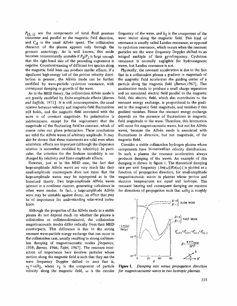
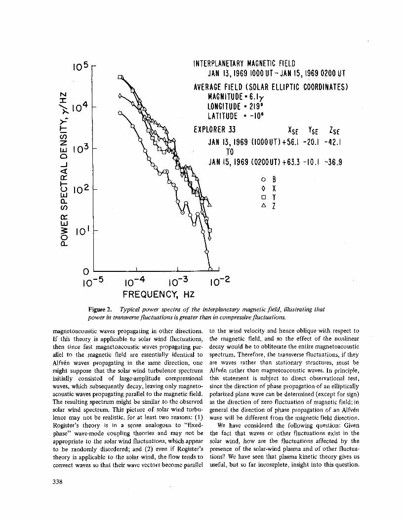
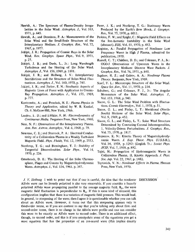
For example, we may inquire what role nonlinear processes play in determining the power spectra of magnetic fluctuations near 1 AU. Figure 2 shows typical power spectra from Explorer 33. Although there is disagreement among observers about the detailed char- acter of interplanetary fluctuations, and in particular of their power spectra, certain features seem to be estab- lished as typical. One such feature, indicated here, is the fact that the power in fluctuations of the magnitude of the magnetic field is normally smaller than the power in fluctuations of direction by about a factor of 10. These fluctuations could be due to stationary structures or to waves. The point to be emphasized at the moment is that to the extent that these fluctuations are waves, they must be either (1) AlfvCn waves, or (2) magnetoacoustic waves propagating very nearly parallel to the magnetic field. They cannot be magnetoacoustic waves propa- gating obliquely to the magnetic field, because then the power in fluctuations of magnitude would be compa- rable to that in fluctuations of the various components.

It is further agreed that correlations of magnetic and plasma fluctuations indicate that AlfvCn waves are often present in the interplanetary medium at 1 AU. On the other hand, there are no reported observations of magnetoacoustic waves. This fact, together with the fact that power in directional fluctuations is usually much greater than in magnitude fluctuations, indicates that obliquely propagating magnetoacoustic waves are

present, if at all, at intensities considerably lower than the intensities of transverse waves. The relative absence of compressive waves is easily understood in terms of the linearized theory, which tells us that magnetoacoustic waves are Landau damped while. AlfvCn waves are not. We have further noted that the Vlasov-Maxwell equa- tions admit large-amplitude AlfvCn wave solutions. Unless for some reason nonlinear effects inhibit the magnetoacoustic Landau damping, the above picture is self-consistent as far as it goes. On the other hand, it is possible that several nonlinear effects could provide an alternate explanation of the dominance of AlfvCn over magnetoacoustic waves at 1 AU.

One obvious possibility is that decay into other, possibly higher frequency, wave modes, rather than Landau damping, accounts for the relative absence of magnetoacoustic waves. The details of such a process have never been analyzed, at least in a context that is clearly appropriate for solar wind fluctuations. However, it is possible to make at least crude order-of-magnitude estimates of nonlinear effects. Since the solar wind usually appears randomly disordered, rather than orga- nized into neatly ordered wave packets, it seems reasonable to ask what one would expect from the “random-phase” approximation of weak-turbulence theory [Tsytovich, 1970; Sagdeev and Galeev, 19691. in this approximation one expects the rate r ~ r , of non- linear decay from one mode into another to be of order

where o is the circular frequency of the wave, AB is the wave amplitude, and B is the magnetic field strength. This expression should be taken as an upper limit on I’YNL I , and even this upper limit is uncertain by at least a factor of 10. If we take ABfB - 0.1, then ~ ’ Y N L I ~ 0.01 a. Hence, it seems plausible that a wave in the solar wind might be significantly modified by non- linear processes in 100 wave periods or less.

Therefore, large-amplitude magnetoacoustic waves may undergo significant dissipation by nonlinear decay into other wave modes, as well as by Landau damping. On the other hand, why do the transverse waves not decay into compressive waves, resulting in a sizable intensity of compressive waves? A tentative answer is that the magnetoacoustic Landau damping rate I ’yo I >> I r ~ r , I; if this is so, the nonlinear decay of transverse waves would be strongly inhibited. Another interesting possibility is the following. Recent theoreti- cal work by Rogister [I9701 suggests that magneto- acoustic waves propagating along the magnetic field may be much more stable against nonlinear decay than

337

I N T E R P LA N ETA R Y MAG N E TI C FI E L D JAN 13,1969 1000 UT - JAN 15,1969 0200 UT

AVERAGE FIELD (SOLAR ELLIPTIC COORDINATES) MAGNITUDE 6 . l y LONGITUDE = 219” LATITUDE -IO0

EXPLORER 33 XSE YSE ZSE JAN 13, 1969 (1000UT) t56 . l -20.1 -42.1

TO 15, 1969 (0200UT) t63.3 -10.1 -36.9

IO-^ IO-^ I 0-3 io-* FREQUENCY, HZ

Figure 2. power in transverse fluctuations is greater than in compressive fluctuations.

Typical power spectra of the interplanetary magnetic field, illustrating that

magnetoacoustic waves propagating in other directions. If this theory is applicable to solar wind fluctuations, then since fast magnetoacoustic waves propagating par- allel to the magnetic field are essentially identical to Alfv6n waves propagating in the same direction, one might suppose that the solar wind turbulence spectrum initially consisted of large-amplitude compressional waves, which subsequently decay, leaving only magneto- acoustic waves propagating parallel to the magnetic field. The resulting spectrum might be similar to the observed solar wind spectrum. This picture of solar wind turbu- lence may not be realistic, for at least two reasons: (1) Rogister’s theory is in a sense analogous to “fiied- phase” wave-mode coupling theories and may not be appropriate to the solar wind fluctuations, which appear to be randomly disordered; and (2) even if Rogister’s theory is applicable to the solar wind, the flow tends to convect waves so that their wave vectors become parallel

to the wind velocity and hence oblique with respect to the magnetic field, and so the effect of the nonlinear decay would be to obliterate the entire magnetoacoustic spectrum. Therefore, the transverse fluctuations, if they are waves rather than stationary structures, must be AlfvCn rather than magnetoacoustic waves. In principle, this statement is subject to direct observational test, since the direction of phase propagation of an elliptically polarized plane wave can be determined (except for sign) as the direction of zero fluctuation of magnetic field; in general the direction of phase propagation of an AlfvCn wave will be different from the magnetic field direction.

We have considered the following question: Given the fact that waves or other fluctuations exist in the solar wind, how are the fluctuations affected by the presence of the solar-wind plasma and of other fluctua- tions? We have seen that plasma kinetic theory gives us useful, but so far incomplete, insight into this question.

338

For example, we have seen that of the five classes of magnetohydrodynamic fluctuations only two, the Alfve’n wave and the tangential pressure balance, are likely to exist in appreciable quantity in the micro- structure of the wind. On the other hand, it is quite conceivable that nonlinear effects significantly modify the fluctuation spectra, but in ways that are obscure at present.

SOURCES OF THE FLUCTUATIONS Even if we had a complete knowledge of the intrinsic properties of solar wind fluctuations, we could not explain the observed fluctuations without knowledge of their sources. Obviously, the sources of stationary structures and of hydromagnetic waves would be very different. Nevertheless, in both cases possible sources may be conveniently placed into three broad classes: (1) the source is at or near the sun; (2) the source is some large-scale process in the interplanetary medium far from the sun; and (3) the source is some instability intrinsic to the solar wind flow far from the sun.

One area in which considerable systematic study has been made deals with the possibility that solar wind fluctuations at 1 AU are stationary structures, origi- nating at the sun, which are convected out in the wind [Siscoe, 1970;Siscoe and Finley, 1969,1970; Carovillano and Siscoe, 19691. These fluctuations are stationary in the local rest frame of the solar wind, but they also corotate with the sun, like the magnetic sector structure. However, these fluctuations involve the large-scale struc- ture of the wind, and may not have a very direct relation with the microstructure of the wind. Nevertheless, stationary microstructures may in fact originate at the sun. Thin, twisted filaments (of thickness -lo6 km) or other topological arrangements of magnetic field coming from the sun have been suggested [Ness, 1968; Burlaga, 19691 . Such an arrangement of stationary structures is a plausible consequence of the random walk of field lines rooted in the solar supergranulation [Jokipii and Parker, 19691. In addition, there is some direct evidence that the statistical properties of stationary structures do not vary much between. about 0.8 and 1.0 AU [Burlaga, 1971 ] , which suggests that their source is nearer the sun than 0.8 AU. In particular, this conclusion is consistent with the hypothesis of solar origin of stationary struc- tures.

It is also possible that stationary structures in the interplanetary medium could originate in the relaxation of some large-scale dynamical process or instability that takes place far from the sun. One possibility would be that stationary structures originate in regions of inter- action between fast and slow streams; however, Burlaga

[1971] suggests that this hypothesis is not supported by observational data. Otherwise, the possible nonsolar origin of stationary fluctuations seems not to have been studied in detail.

Consider now the possible sources of hydromagnetic waves. The most obvious hypothesis is that the waves originate at the sun itself. This idea very naturally explains the recent observations that a substantial fraction of the power in solar wind fluctuations may be identified with Alfvin waves whose propagation direc- tion relative to the plasma is away from the sun [Belcher et al., 1969; Belcher and Davis, 19711. If one assumes this wave efflux to be distributed in a spherically symmetric fashion, the net energy efflux is -3 X 1024ergs/sec, small compared with the estimated 5 X ergs/sec in waves that heat the inner corona [Osterbrock, 19611 . In addition, only Alfvin waves originating near the sun would be able to reach the orbit of earth, because of the strong Landau damping of magnetoacoustic waves. The wave periods (in the space- craft frame) range from -2 hr down at least to 10 min (and probably less); Alfvin wave intensities tend to be higher in fast solar wind streams than in slow ones. All these properties (propagation direction, wave intensity, wave mode, wave period, and intensity-flow speed correlation) are qualitatively consistent with the inter- pretation of these waves as the remnants of a hydromag- netic wave flux and the coronal base, which supplies a significant part of the solar wind energy.

Another large-scale process that may very well be a strong source of hydromagnetic waves in the solar wind is the collision between fast and slow streams. Most waves from this source would be generated in the region from 0.5 to 3 AU [Jokipii and Davis, 19691. Observa- tions indicate that the interaction regions are highly disturbed, with a large amount of power in compressive fluctuations [Belcher and Davis, 197 I]. Presumably these compressive fluctuations are at least partly magnet- oacoustic waves, which are Landau damped before they can propagate far from the interaction region. The wave dissipation produces heating of the gas; the heating appears to be restricted to the locality of the interaction region, at least at 1 AU [Burlaga and Ogilvie, 1970; Belcher and Davis, 19 7 1 ] .

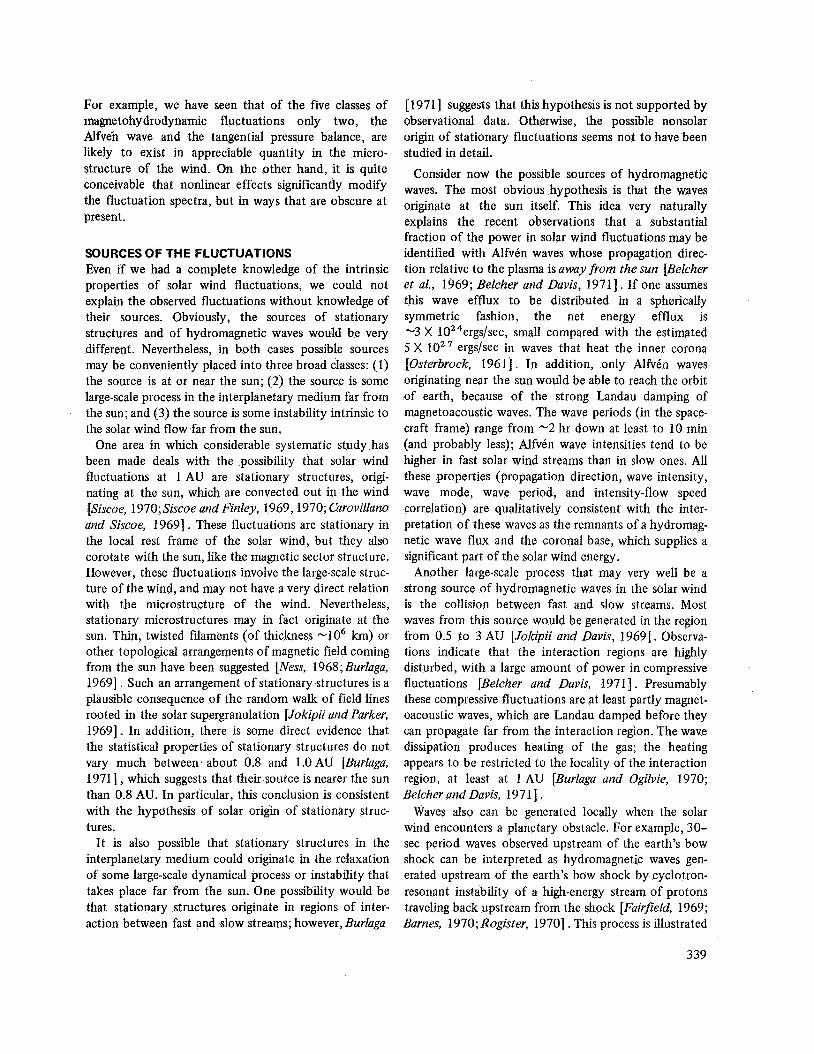
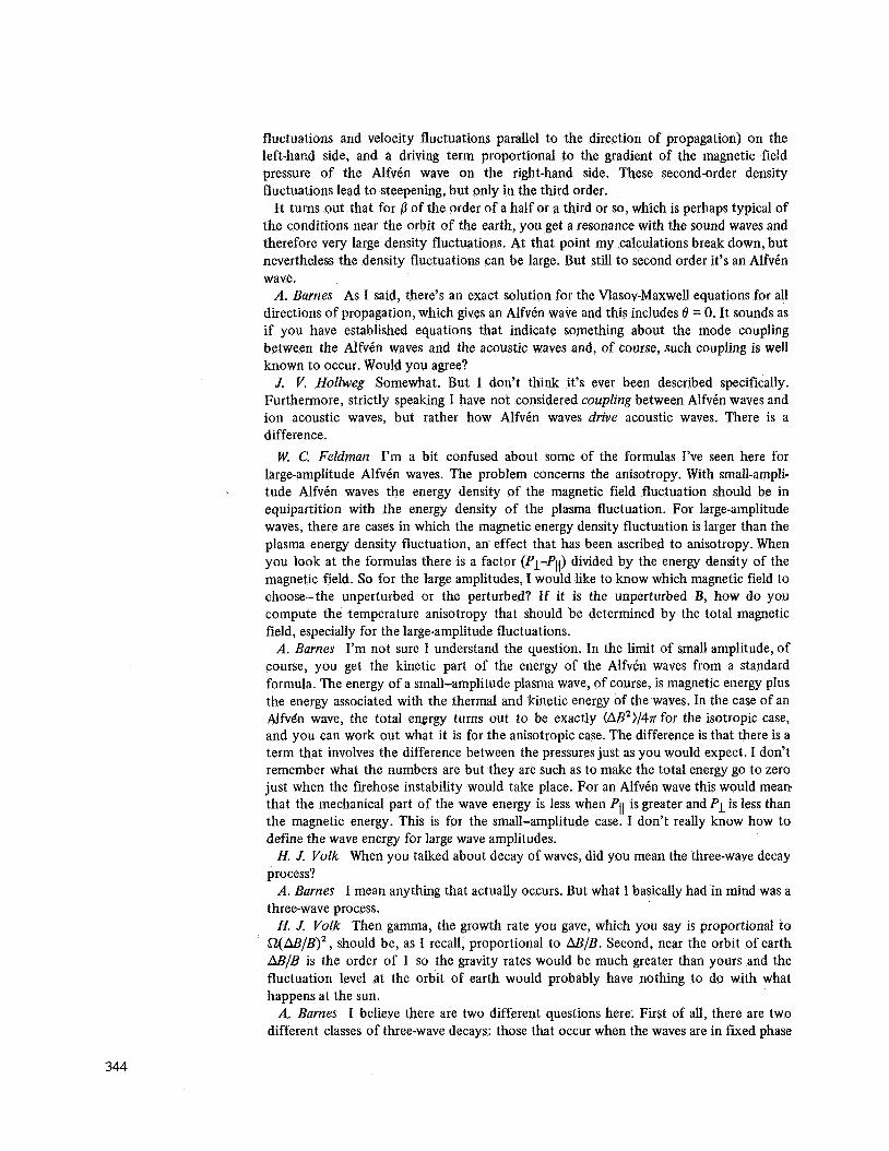
Waves also can be generated locally when the solar wind encounters a planetary obstacle. For example, 30- sec period waves observed upstream of the earth’s bow shock can be interpreted as hydromagnetic waves gen- erated upstream of the earth’s bow shock by cyclotron- resonant instability of a high-energy stream of protons traveling back upstream from the shock [Fairfield, 1969; Barnes, 1970; Rogister, 19701 . This process is illustrated

339

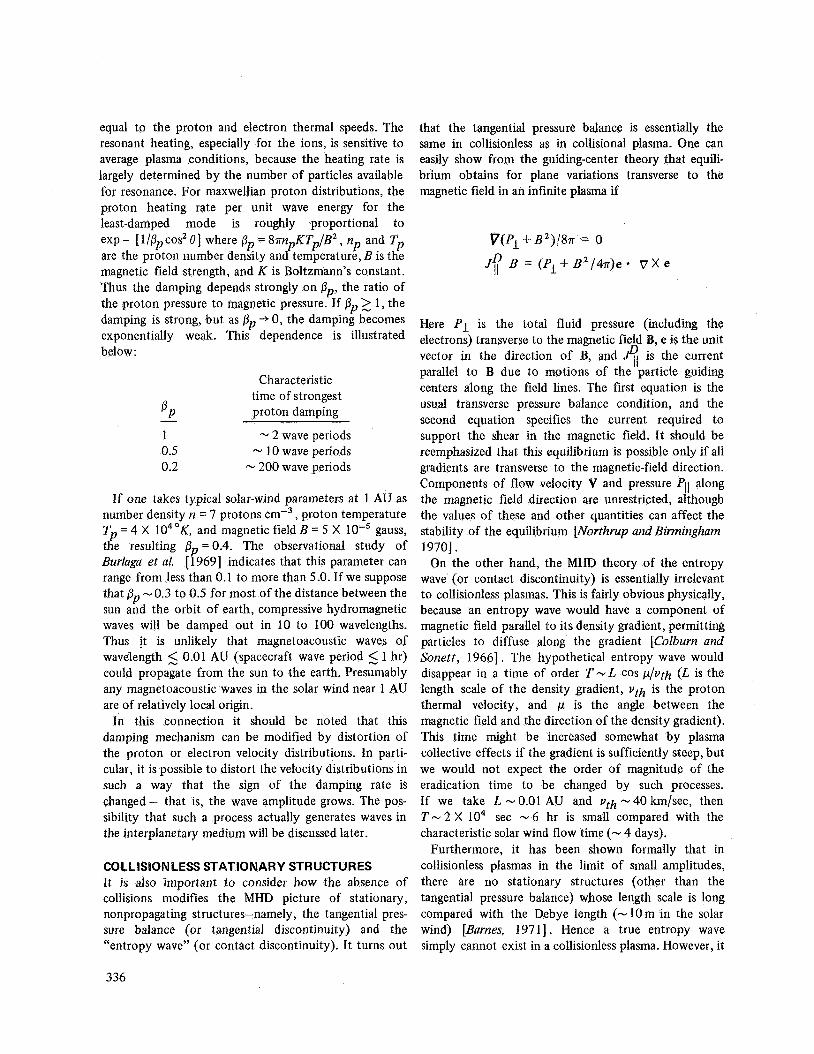
in figure 3. Waves generated at point B upstream are convected back downstream toward the bow shock, resulting in a region of enhanced turbulence. It should be pointed out that an alternate explanation of these waves is that they are whistlers generated at the bow shock and essentially standing in the wind, so that their frequency is Doppler shifted to the observed value of Perez and Northrop [1970]. This particular question, as

BOW MAGNETOPAUSE CUnPV

6 TO SUN

SOLAR WIND FLOW DIRECTION

TURBULENCE

Figure 3. Schematic representation of generation of hydromagnetic waves upstream of the earth’s bow shock, by protons streaming from the shock. Straight solid lines represent interplanetary magnetic field lines.

well as questions about the character of other inter- esting, high frequency waves upstream of the bow shock, has not yet been definitely resolved. In any case, it seems clear that waves should be generated locally in the solar wind whenever it encounters a planetary obstacle. Also, the fact that waves and, very likely, distorted particle velocity distributions exist upstream of the earth‘s bow shock emphasizes that caution must be used in interpreting solar wind data from earth orbiting spacecraft. In particular, data taken at times when the spacecraft is located on an interplanetary magnetic field line that intersects the bow shock can be contaminated by shock-produced effects.

Besides the previously mentioned sources of hydro- magnetic waves in the solar wind, it is probable that such waves can be produced by a variety of processes intrinsic to the flow of the wind. The possible influence of nonlinear effects on the solar wind fluctuation spectrum has already been mentioned. Another possibility would be the Kelvin-Helmholtz instability, which can some- times occur when two streams in tangential pressure

balance slip past one another. However, the observa- tional study of Burlaga and Ogilvie [ 1970) indicates that this instability is probably not a significant source of heating in the wind, so that this mechanism is probably not a significant source of waves in the wind.

Another interesting possible source of hydromagnetic waves is microinstability of solar wind electrons due to distortion of their velocity distribution by thermal conduction [Forslund, 1970; Perkins and Spight, 19701. In particular, Forslund [1970] has suggested that two hydromagnetic wave modes can be generated in this way. For example, it is conceivable that ion-acoustic waves, including the slow-mode hydromagnetic wave, could be generated by conductive instability if the ratio of electron to proton temperature is sufficiently high. Forslund has suggested that this process occurs at a heliocentric distance r = 10 R, for temperature distribu- tions of the bare two-fluid model of the solar wind. On the other hand, this particular instability probably would not occur for temperature distribptions corre- sponding to models with external heating. Forslund has also suggested that fast-mode hydromagnetic waves might be generated by conductive instability in the vicinity of 1 AU, by the inverse of the Landau-damping process discussed earlier. However, it seems unlikely that any fast-mode waves produced in this way would be easily observable, for several reasons. First, Forslund‘s mechanism generates fast-mode waves only for a fairly narrow range of propagation directions (51 5”); waves produced in this way would eventually be refracted outside this narrow production cone, into other direc- tions where Landau damping occurs, and therefore such waves probably would not be observable long after they were generated. Second, the fastest growth rate of this process occurs for waves whose frequency is of the order of the proton gyrofrequency; and since the growth time of a microinstability is usually also a measure of its quenching time, it is likely that very little power in hydromagnetic waves will be generated by the insta- bility. Probably the main effect of this instability would be to keep the electron velocity distribution near the marginally stable configuration, possibly with an asso- ciated “fizz” of noise whose characteristic frequency is comparable to the proton gyrofrequency. Altogether, then, it appears that although the thermal conduction instabilities considered by Forslund may conceivably have nonnegligible effects on thermal conduction and electron-proton energy exchange, they are not likely to produce readily observable hydromagnetic waves in the solar wind.

It is conceivable that other microinstabilities could generate hydromagnetic waves in the solar wind. For

340

example, instabilities like the firehose associated with pressure anisotropy can generate hydromagnetic waves, at least in principle. Waves by anisotropy would be generated preferentially in higher-fi regions of the wind. According to the work of Burlaga et al. [ 19691 regions of high fi tend to be associated with enhanced micro- fluctuations, which would be consistent with their being waves generated by anistropyddven microinstabilities. On the other hand, Belcher and Davis [ 19711 argue that enhanced fluctuations are better correlated with colliding-stream regions (which are often, but not always, regions of high p), and that the fluctuations are generated by the large-scale, stream-stream interaction rather than anisotropy. From a theoretical standpoint, anisotropy-driven instabilities generate higher frequency or shorter wavelength waves more abundantly than hydromagnetic waves; probably the main effect of anisotropy-driven instability is to maintain the aniso- tropies in a marginally stable state, and to generate a relatively weak background of high frequency, short wavelength noise.

Altogether, it appears quite likely that most hydro- magnetic waves in the solar wind are generated in large-scale processes. Observations at 1 AU are consistent with the generation of a large fraction of the waves at the sun; in addition, other large-scale processes, notably the collision of fast and slow streams, contribute to the observed fluctuations. Interaction of the wind with a planetary obstacle may account for local generation of hydromagnetic waves. The fluctuation spectrum of the wind may be significantly affected by nonlinear pro- cesses. Other small-scale processes, such as microinstabil- ities, are probably a relatively minor source of hydromagnetic waves.

RELATION TO LARGE-SCALE PROPERTIES OF THE WIND Hydromagnetic waves may influence the large-scale properties of the wind in a number of important ways. For example, heating due to Landau damping of magnetoacoustic waves, whatever their source, can have a significant effect on the flow. It has been shown that a model in which heating is due to thermal conduction and dissipation of an efflux of magnetoacoustic waves of -4-min period generated at the sun can explain the observed correlation between proton temperature and flow speed at 1 AU for a large range of flow speeds [Barnes et al., 1971; Hartle and Barnes, 1971; Barnes and Hartle, 19711. Jokipii and Davis [1969] have suggested that the damping of magnetoacoustic waves generated by the collision of fast and slow streams is significant for solar wind heating. Observational evidence

indicates that this process probably produces local rather than global heating at 1 AU [Burlaga and Ogilvie, 19701 ; Belcher and Davis, 19711, but this process may well produce larger scale effects beyond 1 AU.

Besides heating, the dissipation and even the simple propagation of hydromagnetic waves produce a force on the wind. It is possible that this sort of “radiation pressure” has a significant effect on the flow of the wind, especially if it acts in the region of supersonic flow. Belcher [ 197 11 has developed a polytropic model of the solar wind which includes pressure due to the propagation of AlfvCn waves outward from the sun. These waves do not damp locally, but gradually lose energy because they do work on the wind as they propagate outward. Although that model in its present form is probably not realistic in detail, it does show that radiation pressure from hydromagnetic waves may sig- nificantly accelerate the wind.

Fluctuations in the solar wind are related to many other problems of great current interest. Hydromagnetic waves or other fluctuations may participate in the transport of angular momentum from the sun [Schubert and Coleman, 1968: Siscoe, 19701. Scattering and diffusion of cosmic rays are caused by fluctuations in the interplanetary medium [Jokipii, 197 11 . Scintillation and scattering of signals from radio sources are produced by interplanetary fluctuations [Hewish and Dennison, 1967; Cohen et al., 1967; Jokipii and Hollweg, 1970; Hewish, 19711. Some of these problems, which are far beyond the scope of this discussion, are considered in other chapters.

One last topic should be mentioned briefly here. There are numerous observations of interplanetary fluctuations of shorter length scale and higher frequency than hydromagnetic-scale fluctuations. [see review by ScarA 19701. By combination of higher frequency magnetic and electric field measurements, some progress has been made in identifying the modes of various fluctuations, at least to the extent of distinguishing electrostatic from electromagnetic oscillations.

Higher frequency waves (period -2 sec) as well as hydromagnetic waves are generated in the upstream solar wind by the earth’s bow shock [Russell et al., 19711. Probably the noise generated by microinstabilities due to anisotropy or to saturation of thermal conduction will be predominantly at frequencies comparable to or greater than the proton gyrofrequency. High-frequency noise will probably be found in most regions of rapid change, like shock fronts or colliding-stream regions.

Although the smaller-scale fluctuations normally con- tribute a small fraction of the total fluctuation energy in the wind, such fluctuations probably can have some

34 1

effect on the large-scale structure of the wind. For beyond a heliocentric distance of about 10 R,, wave- particle interactions probably have significant influence on transport phenomena, perhapk completely domi- nating Coulomb collisions [Eviatar and Schulz, 1970; Newrnan and Sturrock, 19691. Modification of thermal conduction and proton-electron energy exchange by various collisionless mechanisms have been considered [Forslund, 1970; Perkins and Spight, 19701. Eviatar and Wolf [ 1968 J have discussed a possible collisionless viscous interaction between the solar wind and the earth’s magnetosphere. It is conceivable that some such viscous mechanism could affect the heating, and espe- cially the angular momentum transport of the wind.

To conclude, it is clear that the study of microscale fluctuations, both of hydromagnetic and smaller scale, is of great importance. The microscale fluctuations present an opportunity to directiy observe waves in a plasma whose fluid pressure is not small compared with its magnetic pressure. Furthermore, observed fluctuations may provide major clues for understanding important large-scale effects in the solar wind. Considerable prog- ress, partly theoretical but maifdy observational, has been made in these areas in the past several years. I think that we may expect even greater advance in our understanding of the nature, origin, and effects of solar wind fluctuations in the near future. Again, most of this progress will probably come from observation, partly from new instrumentation, new spacecraft missions, partly from analysis of data from existing spacecraft, and hopefully from multiple satellite experiments.

ACKNOWLEDGEMENTS I am grateful to Dr. Bruce Smith for providing the power spectra of figure 2, and to Dr. Patrick Cassen for his comments on the first draft of this review.

REF E RENCES Barberio-Corsetti, P.: Entropy Mode Identification. Bull.

Arner. Phys. SOC., Vol. 14,1969, p. 1019. Barnes, A.: Collisionless Damping of Hydromagnetic

Waves. Phys. Fluids, Vol. 9, 1966, p. 1483. Barnes, A.: Stochastic Electron Heating and Hydromag-

netic Wave Damping. Phys. Fluids, Vol. 10, 1967, p. 2427.

Barnes, A.: Theory of Generation of Bow-Shock- Associated Hydromagnetic Waves in the Upstream Interplanetary Medium. Cosmic Electrodyn., Vol. 1, 1970, p. 90.

Barnes, A.; and Suffolk, G. C. J.: Relativistic Kinetic Theory of the Large-Amplitude Transverse AlfvCn Wave. J. Plasma Phys., in press, 1971.

Barnes, A.: Theoretical Constraints on the Micro-scale Fluctuations in the Interplanetary Medium. J. Geophys. Res., in press, 1971.

Barnes, A.; Hartle, R. E.; and Bredekamp, J. H.: On the Energy Transport in Stellar Winds. Astrophys. J., Vol. 166,1971, p. L53.

Barnes, A; and Hartle, R. E.: Model for Energy Transfer in the Solar Wind: Model Results (proceedings of this meeting), 197 1.

Belcher, J. W.: Alfvhnic Wave Pressures and the Solar Wind. Astrophys. J., Vol. 68,1971, p. 509.

Belcher, J. W.; and Davis, L., Jr.: Large Amplitude Alfvbn Waves in the Interplanetary Medium: 11. J. Geophys. Res., Vol. 76, 1971, p. 3534.

Belcher, J. W.; Davis, L., Jr.; and Smith, E. J.: Large Amplitude Alfven Waves in the Interplanetary Medium: Mariner 5. J. Geophys. Res., Vol. 74, 1969, p. 2302.

Burlaga, L. F.: Directional Discontinuities in the Interplanetary Magnetic Field. Solar Phys., Vol. 7, 1969, p. 54.

Burlaga, L. F.: On the Nature and Origin of Directional Discontinuities. J. Geophys. Res., Vol. 76, 1971, p. 4360.

Burlaga, L. F.; and Ogilvie, K. W.: Heating of the Solar Wind. Astrophys. J., Vol. 159,1970, p. 659.

Burlaga, L. F.; Ogilvie, K. W.; and Fairfield, D. H.: Microscale Fluctuations in the Interplanetary Mag- netic Field. Astrophys. J., Vol. 155, 1969, p. L171.

Carovillano, R. L.; and Siscoe, G. L.: Corotating Structure in the Solar Wind. Solar Phys., Vol. 8 , 1969, p. 401.

Cohen, M. H.; Gundermann, E. J.; Hardebeck, H. E.; and Sharp, L. E.: Interplanetary Scintillations, 2, Observa- tions. Astrophys. J., Vol. 147, 1967, p. 449.

Colburn, D. S.; and Sonett, C. P.: Discontinuities in the Solar Wind. Space Sci. Rev., Vol. 5, 1966, p. 439.

Eviatar, A.; and Schulz, M.: Ion-Temperature Aniso- tropies and the Structure of the Solar Wind. Planet. SpaceSci., Vol. 18, 1970, p. 321.

Eviatar, A.; and Wolf, R. A.: Transfer Processes in the Magnetopause. J. Geophys. Res., Vol. 73, 1968, p. 5561.

Fairfield, D. H.: Bow-Shock-Associated AlfvCn Waves in the Upstream Interplanetary Medium. J. Geophys. Res., Vol. 74, 1969, p. 3541.

Forslund, D. W.: Instabilities Associated with Heat Conduction in the Solar Wind and Their Conse- quences. J. Geophys. Res., Vol. 75, 1970, p. 17.

Hartle, R. E.; and Barnes, A.: Model for Energy Transfer in the Solar Wind: Formulation of Model (proceed- ings of this meeting), 1971.

342

Hewish, A.: The Spectrum of Plasma-Density Irregu- larities in the Solar Wind. Astrophys. J., Vol. 163, 1971, p. 6 4 5 .

Hewish, A.; and Dennison, P. A.: Measurements of the Solar Wind and the Small-scale Structure of the Interplanetary Medium. J. Geophys. Res., Vol. 72, 1967, p. 1977.

Jokipii, J. R.: Propagation of Cosmic Rays in the Solar Wind. Rev. Geophys. Space Phys., Vol.9, 1971, p. 27.

Jokipii, J. R.; and Davis, L., Jr.: Long Wavelength Turbulence and the Heating of the Solar Wind. Astrophys. J., Vol. 156, 1969, p. 1101.

Jokipii, J. R.; and Hollweg, J. V.: Interplanetary Scintillations and the Structure of Solar-Wind Fluc- tuations. Astrophys. J., Vol. 160, 1970, p. 745.

Jokipii, J. R.; and Parker, E. N.: Stochastic Aspects of Magnetic Lines of Force with Application to Cosmic- Ray Propagation. Astrophys. J., Vol. 155, 1969,

Kantrowitz, A.; and Petschek, H. E.: Plasma Physics in Theory and Application, edited by W. B. Kunkel, Ch. 6. McGraw-Hill, New York, 1966.

Landau, L. D.; and Lifshitz, E. M.: Electrodynamics of Continuous Media. Pergamon Press, New York, 1960.

Ness, N. F.: Observations of the Interplanetary Plasma. Ann. Rev. Astron. Astrophys., Vol. 6, 1968, p. 79.

Newman, C. E.; and Sturrock, P. A.: Electrical Conduc- tivity of a Collisionless Plasma in a Weakly Turbulent Magnetic Field. Phys. Fluids, Vol. 12, 1969, p. 2553.

Northrop, T. G.; and Birmingham, T. J.: Stability of Tangential Discontinuities. Solar Phys., Vol. 14, 1970, p. 226.

p. 777.

Perez, J. K.; and Northrop, T. G.: Stationary Waves Produced by the Earth’s Bow Shock. J. Geophys. Res., Vol. 75, 1970, p. 601 1.

Perkins, F. W.; and Spight, C.: Magnetic Field Effects on the Ion-Acoustic Instability in the Solar Wind (abstract). EOS, Vol. 51, 1970, p.412.

Rogister, A.: Parallel Propagation of Nonlinear Low Frequency Waves in High 0 Plasma, submitted for publication, 1970.

Russell, C. T.; Childers, D. D.; and Coleman, P. J., Jr.: OGO-5 Observations of Upstream Waves in the Interplanetary Medium: Discrete Wave Packets. J. Geophys. Res., Vol. 76, 1971, p. 845.

Sagdeev, R. Z.; and Galeev, A. A.: Nonlinear Plasma Theory. Benjamin, New York, 1969.

Scarf, F. L.: Microscopic Structure of the Solar Wind. Space Sci. Rev., Vol. 11, 1970, p. 234.

Schubert, G.; and Coleman, P. J., Jr.: The Angular Momentum of the Solar Wind. Astrophys. J. , Vol. 153,1968, p. 943.

Siscoe, G. L.: The Solar Wind Problem with Fluctua- tions. Cosmic Electrodyn., Vol. 1, 1970, p. 5 1.

Siscoe, G . L.; and Finley, L. T.: Meridional (North- South) Motions of the Solar Wind. Solar Phys., Vol. 9, 1969, p. 452.

Siscoe, G. L.; and Finley, L. T.: Solar Wind Structure Determined by Corotating Coronal Inhomogeneities, 1, Velocity-Driven Perturbations. J. Geophys. Res., Vol. 75, 1970, p. 1817.

Stepanov, K. N.: Kinetic Theory of Magnetohydrody- namic Waves. J. Exp. Theor. Phys. (U.S.S.R.), Vol. 34, 1958, p. 1292; (English Tr.: Soviet Phys. JETP, Vol. 7, 1958, p. 892.

Tajiri, M.: Propagation of Hydromagnetic Waves in Collisionless Plasma, 11, Kinetic Approach. J. Phys.

Osterbrock, D. E.: The Heating of the Solar Chromo- sphere, Plages and Corona by Magnetohydrodynamic Waves. Astrophys. J., Vol. 134, 1961, p. 347.

SOC. Jap. Vol. 22, 1967, p. 1482.

Press, New York, 1970. Tsytovich, V. N.: Nonlinear Effects in Plasma, Plenum

J. V. Hollweg I wish to point out that if one is careful, the idea that the nonlinear DISCUSSION Alfvin wave can be linearly polarized is also very reasonable. If you consider a linearly polarized Alfvin wave propagating parallel to the average magnetic field, Bo, the wave magnetic field fluctuation is perpendicular to Bo. If this is some kind of sinusoid, this configuration implies that there is a variation of magnetic field pressure. This would lead, in general, to steepening of the wave; then I agree it is questionable whether you can talk about an Alfvin wave. However, it turns out that this steepening appears only in third-order terms, so if you are content to say that you’re talking only about first- and second-order terms, there is no change in the AlfvCn wave profile and one can consider this wave to be exactly an Alfvdn wave to second order. There is an additional effect, though, to second order, and this is if you manipulate some of the equations you get a wave equation that has the properties of an ion-sound wave (this implies density

343

fluctuations and velocity fluctuations parallel to the direction of propagation) on the left-hand side, and a driving term proportional to the gradient of the magnetic field pressure of the Alfv6n wave on the right-hand side. These second-order density fluctuations lead to steepening, but only in the third order.

It turns out that for 0 of the order of a half or a third or so, which is perhaps typical of the conditions near the orbit of the earth, you get a resonance with the sound waves and therefore very large density fluctuations. At that point my calculations break down, but nevertheless the density fluctuations can be large. But still to second order it’s an Alfvh wave.

A . Barnes As I said, there’s an exact solution for the Vlasov-Maxwell equations for all directions of propagation, which gives an Alfvh wave and this includes 6 = 0. It sounds as if you have established equations that indicate something about the mode coupling between the Alfvh waves and the acoustic waves and, of course, such coupling is well known to occur. Would you agree?

J. K Hollweg Somewhat. But I don’t think it’s ever been described specifically. Furthermore, strictly speaking I have not considered coupling between Alfvh waves and ion acoustic waves, but rather how Alfvkn waves drive acoustic waves. There is a difference. W. C. Feldman I’m a bit confused about some of the formulas I’ve seen here for

large-amplitude Alfvh waves. The problem concerns the anisotropy. With small-ampli- tude Alfvh waves the energy density of the magnetic field fluctuation should be in equipartition with the energy density of the plasma fluctuation. For large-amplitude waves, there are cases in which the magnetic energy density fluctuation is larger than the plasma energy density fluctuation, an effect that has been ascribed to anisotropy. When you look at the formulas there is a factor (Pl-PIl) divided by the energy density of the magnetic field. So for the large amplitudes, I would like to know which magnetic field to choose-the unperturbed or the perturbed? If it is the unperturbed B, how do you compute the temperature anisotropy that should be determined by the total magnetic field, especially for the large-amplitude fluctuations.

A. Barnes I’m not sure I understand the question. In the limit of small amplitude, of course, you get the kinetic part of the energy of the Alfvkn waves from a standard formula. The energy of a small-amplitude plasma wave, of course, is magnetic energy plus the energy associated with the thermal and kinetic energy of the waves. In the case of an Alfv6n wave, the total energy turns out to be exactly U 2 ) / 4 n for the isotropic case, and you can work out what it is for the anisotropic case. The difference is that there is a term that involves the difference between the pressures just as you would expect. I don’t remember what the numbers are but they are such as to make the total energy go to zero just when the firehose instability would take place. For an Alfvhn wave this would mean. that the mechanical part of the wave energy is less when Pi1 is greater and PI is less than the magnetic energy. This is for the small-amplitude case. I don’t really know how to define the wave energy for large wave amplitudes.

H. J. Volk When you talked about decay of waves, did you mean the three-wave decay process?

A. Barnes I mean anything that actually occurs. But what I basically had in mind was a three-wave process.

H. J. Volk Then gamma, the growth rate you gave, which you say is proportional to S2(AB/B)2, should be, as I recall, proportional to AB/B. Second, near the orbit of earth AB/B is the order of 1 so the gravity rates would be much greater than yours and the fluctuation level at the orbit of earth would probably have nothing to do with what happens at the sun.

A. Barnes I believe there are two different questions here. First of all, there are two different classes of three-wave decays: those that occur when the waves are in fured phase

344

and those that occur when the waves are in random phase. For fixed phase waves the growth rate is proportional to AB/B. For random phase it is proportional to (AB/B)2. This, by the way, is essentially the formula that Parker used yesterday for a related process, which you could look at as the three-wave decay between Alfvh waves, magnetoacoustic waves, and maybe tangential pressure balance or something like that. So if you assume that the appropriate theory to use is for the solar wind random phase theory, then is correct. Second, I think I said that the amount of power in the fluctuations at earth AB/B can range from less than 0.1 to 1.0. Perhaps some of the experimentalists would like to comment on this, but it seems to me that from the data I have seen that AB/B on the order of 0.1 is typical, though certainly it can be as great as 1.0, in which case the nonlinear decay may be much larger than I said it would be. The decay is proportional to after all, and so it's a very sensitive function that varies quite a bit.

The other point, however, is that the expression I wrote is an upper limit. It doesn't include the dynamics, the cross section, for the wave-wave interaction, and it may be that a detailed analysis of these things would show smaller growth rates in some cases.

N. F. Ness In connection with the question from observational data, if the nuctuations are normalized, and if you were to use a discontinuity as defined by Siscoe et al., the threshold value was 4 y out of an ambient field average of something like 5 y. If you were to use the 30" definition or the larger of Burlaga's, then you would have a relative amplitude ratio of 0.5. If you look at the time scale plots of Belcher and Davis (figs. 1,2, p. 383) you find that the fluctuations are of approximately equal amplitudes throughout the ambient magnetic field for the period ranges studied. Generally I think that AB/B at the periods you are considering is on the order of unity. This includes periods up to about 1 hr.

F. C. Michel I have a comment on these damping rates. Basically, there are two simple approximations one can make. One can describe the interplanetary medium as being made up of frozen-in fluctuations that are just convected out. Or one assumes that the medium is homogeneous with superimposed waves. Both of these are extreme approximations. Now, for the frozen-in approximation, at least in the filamentary picture, there are filaments unwinding or moving relative to one another. For example, if all filaments were radial except one that wiggled back and forth, this wiggle would tend to straighten out and behave in a sense as a propagating wave. Whether or not one calls this a wave is a matter of taste. I personally think the filamentary picture is preferable. But, the damping rates come from the picture of a homogeneous plasma and a monochromatic wave. I think that the short times appropriate for the damping time of a uniform plasma wave in a homogeneous medium are not appropriate for the time that it would take the filaments to rearrange and become uniform.

A. Barnes I agree. The time scales I gave for dissipation of hydromagnetic waves are probably quite a bit shorter than those for filaments to rearrange themselves. The latter would be on the order of the flow time between the sun and earth, right? And the homogeneous theory is applicable only if the length scale of the fluctuation is short compared with the scale height of the solar wind.

L. Davis I believe that a reasonable way to investigate whether AB/B is 1.0 or 0.1 is through variance over periods of say 3 hr. I think it's worth trying to make a somewhat finer division than this because I think the effects vary more or less as the square. As I recall, it is rare that the square root of the variance over a period of something like 3 hr approaches the value of 4 or 5 y typical of the field strength. I think AB/B about 0.7 for these very disturbed times is a somewhat better characteristic value than 1. The square of that is 0.5 and on these curves which rise very steeply, the difference between 0.5 and 1 .O for (L?&/B)~ is probably significant.

N. F. Ness I think that the use of the standard deviation to measure AB/B for these

345

nonlinear wave modes is not correct. One should look at the time history and look at the amplitude, peak to peak, relative to the magnitude of the field to obtain a correct e st ima te . COMMENTS L? W. Forslund Barnes mentioned (p. 340) that there are a number of micro- instabilities in the solar wind that occur due to the heat flux and velocity space anisotropies. I would like to review briefly some of their properties and how they may arise.

A number of properties of the plasma were described earlier in studies of the large-scale structure of the steady-state solar wind. In particular, there are at least three properties that illustrate how the dynamics of the expansion can cause a departure of the plasma from thermodynamic equilibrium. One simple case is that proton temperature is distinct from that of the electrons because of the weak collisional coupling. A second effect arises if there are few collisions between the proton components-that is, a velocity anisotropy between the components parallel and perpendicular to the magnetic field. This can arise in the electron component also if collisions or wave interactions are sufficiently weak. A third effect arises in any model one chooses-collisionless, exospheric, one-fluid, or even two-fluid magnetohydrodynamic. There exists a heat flux outward from the sun (unless an isothermal approximation is made). This effect appears microscopically as a third moment of the electron and ion distribution functions.

I shall describe briefly how these last two types of velocity space anisotropy give rise to plasma instabilities. In particular, the plasma, if it can, will try to destroy these departures from thermodynamic equilibrium, since they are a free energy sohrce on a microscopic scale. How might one determine the various ways the plasma in the solar wind can tap the free energy, relax closer to an equilibrium thermodynamic state, and in a sense approach the properties of a one-fluid model? The important thing to recall, as Perkins mentioned earlier (Chap. 3, p.213, is that the transport properties of the plasma can be altered due to instabilities. A model analysis shows “feedback” superimposed on the steady-state dynamic expansion of the solar wind with the possibility of giving better agreement with observation of the large scale features. In particular, the recent model of Brandtefal. [1969] illustrates how an alteration of the heat flux, by arbitrarily modifying the transport coefficients, can make the model calculations agree better with observation.

Turning now to the process by which a heat flux may give rise to instabilities, assume a spherically symmetric model including a spiral magnetic field and no net electric charge flow out from the sun. Hence, on the average, the current parallel to the magnetic field is zero, which taken with the fluid equations may be written as

where ill is the parallel current, g1 the electrical conductivity, K , the usual transport coefficient, J/ the angle of B with the radial direction, n the number density, p the pressure, and 0, the electron temperature. For zero current one has to balance the current from the temperature gradient with the current from the effective electric field. The dimensionless parameters that enter into the determination of the transport coefficients AE are complex, but basically they can be thought of as corresponding to the electric field normalized to the runaway field-the field in which the electrons will be accelerated freely. We also define the quantity BT, the ratio of the mean free path for collisions to the scale length of the temperature gradient, in this case the scale length of the solar wind. The zero current condition requires that AE = 0.35 BT. For collisional heat conduction, these two parameters must be small compared to unity, which in fact they are not in the solar wind. As Montgomery has shown (Chap. 3, p.210), there is a significant discrepancy between the observed value of BT and that predicted by Spitzer-Hkm theory.

346

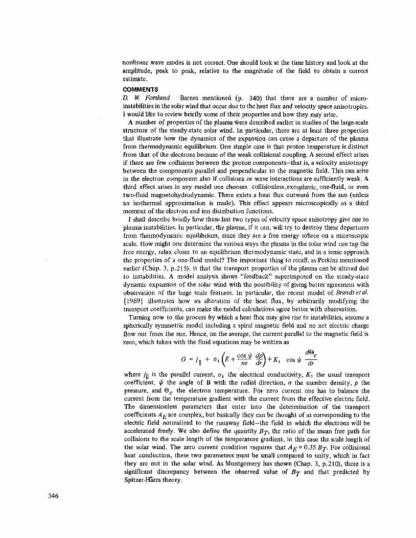
Within linear transport theory the equilibrium electron distribution function is given by

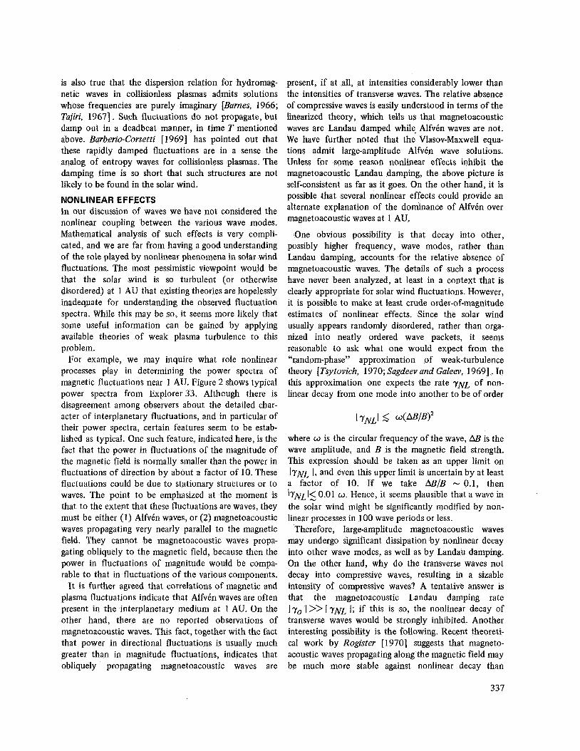
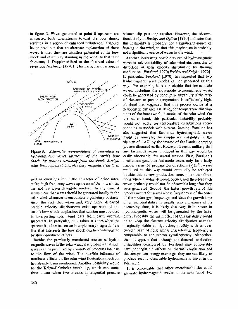
where 6 is the angle of v with respect to the gradients, the function foe@) is the maxwellian distribution, and the transport parameters A E and BT multiply the perturbed distribution functions DE and DT describing the current flow and the heat flux. Figure 1 illustrates the way in which the distribution gives rise to instability. The third moment of

LEFT : SLICE THROUGH f , PARALLEL TO 8 RIGHT: THE REDUCED DISTRIBUTION FUNCTION FJV,,) =/dvLfe

Figure 1. Linearized electron distribution function in a combined electric field and temperature gradient. BT= 0.9, A E = 0.32.

the electron distribution function averaged over velocities perpendicular to B shifts the peak of the distribution away from the protons even though they have a net velocity that matches the proton flow speed. Free energy then exists due to the shift of this peak. That is, if waves can exist in the region between the electron and ion peaks they can extract some of the heat flux energy from the electrons and produce turbulence. We have described here how a heat flux instability can arise for a collisionally driven distribution function, but as Parker pointed out earlier (Chap. 3), collisions are not absolutely necessary for instability to occur. In collisionless exospheric models a distribution function very similar to that in figure 1 can arise. At a given distance from the sun there will be a velocity cutoff for trapping electrons, as Perkins has pointed out (p. 215), due to an electrostatic potential barrier at large radius from the sun and a magnetic mirror at small radius. Above that velocity a flux of escaping electrons gives rise to a shift of the electron peak away from the average velocity, again generating a local source of free energy.

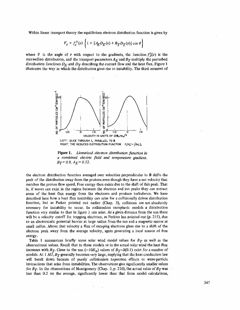
Table 1 summarizes briefly some solar wind model values for BT as well as the observational values. Recall that in these models or in the actual solar wind the heat flux increases with BT. Close to the sun (-lo&,) values of BT-O(O.~) exist for a number of models. At 1 AU, BT generally becomes very large, implying that the heat-conduction law will break down because of purely collisionless expansion effects or wave-particle interactions that arise from instabilities. The observations give significantly smaller values for B T In the observations of Montgomery (Chap. 3,p. 210), the actual value OfBTwas less than 0.2 on the average, significantly lower than that from model calculations,

347

MODEL

HARTLE ond STURROCK 119681

WHANG ond CHANG [I9651

BRANDT et 01. 219691 -2.6 S = 2/5

-0.26 S s2/7 = 450 OBSERVATIONS

T - 1 0 5 4 K , n - 5 c m - 3

10 R, 215 Ron1 A.U.

-0.4 -1.5 e = O0

-0.1 -0.8 too

indicating that the models are actually not very good and should be modified. By reducing the value of BT in their model, Brandtetal. [1969] obtained much better agreement with observations at 1 AU.

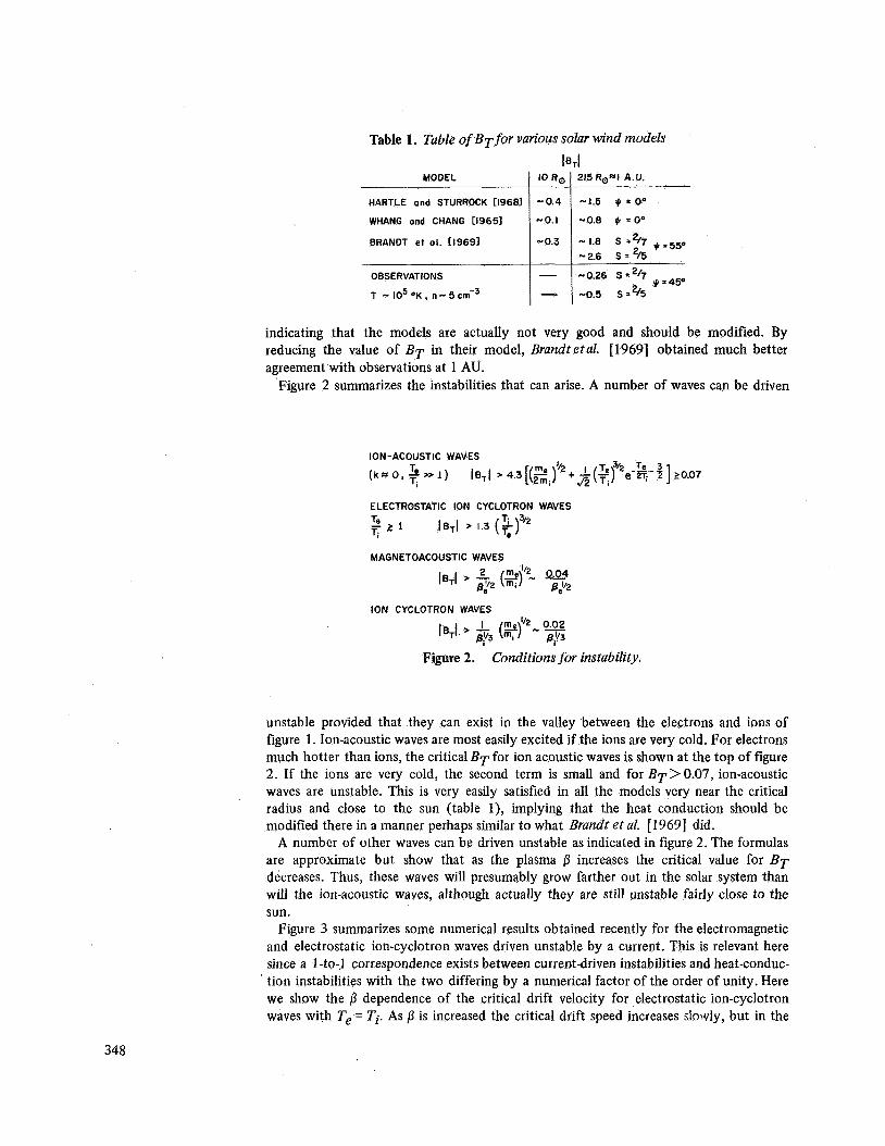
Figure 2 summarizes the instabilities that can arise. A number of waves can be driven

ION-ACOUSTIC

(kn 0, Te >> 1 Ti

WAVES

1 1 % I ' 4.3 [(Zi ELECTROSTATIC ION CYCLOTRON WAVES Te T. 3/2

.?, 1 19~1 > 1.3 (t) MAGNETOACOUSTIC WAVES

t 0 N CYCLOTRON WAVES

Figure 2. Conditions for instability.

3 'f 3 20.07

unstable provided that they can exist in the valley between the electrons and ions of figure 1 . Ion-acoustic waves are most easily excited if the ions are very cold. For electrons much hotter than ions, the critical BT for ion acoustic waves is shown at the top of figure 2. If the ions are very cold, the second term is small and for B ~ > 0 . 0 7 , ion-acoustic waves are unstable. This is very easily satisfied in all the models very near the critical radius and close to the sun (table l), implying that the heat conduction should be modified there in a manner perhaps similar to what Brandt et al. [ 19691 did.

A number of other waves can be driven unstable as indicated in figure 2. The formulas are approximate but show that as the plasma /3 increases the critical value for BT decreases. Thus, these waves will presumably grow farther out in the solar system than will the ion-acoustic waves, although actually they are still unstable fairly close to the sun.

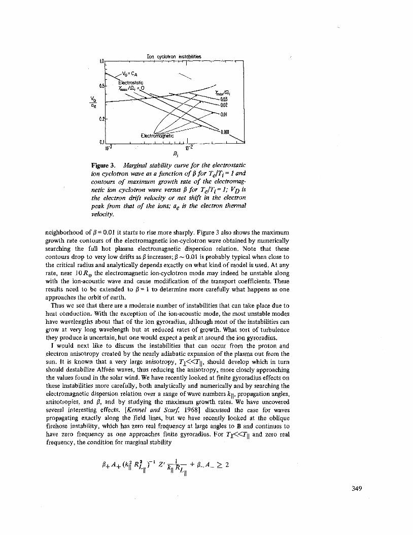
Figure 3 summarizes some numerical results obtained recently for the electromagnetic and electrostatic ion-cyclotron waves driven unstable by a current. This is relevant here since a 1 -to-] correspondence exists between current-driven instabilities and heat-conduc-

' tion instabilities with the two differing by a numerical factor of the order of unity. Here we show the /3 dependence of the critical drift velocity for electrostatic ion-cyclotron waves with Te = Ti. As /3 is increased the critical drift speed increases drwly, but in the

348

Ion cyclotron ustablitis I I

0.5

- "0 ae

0.2

0.1 10-3 10-2

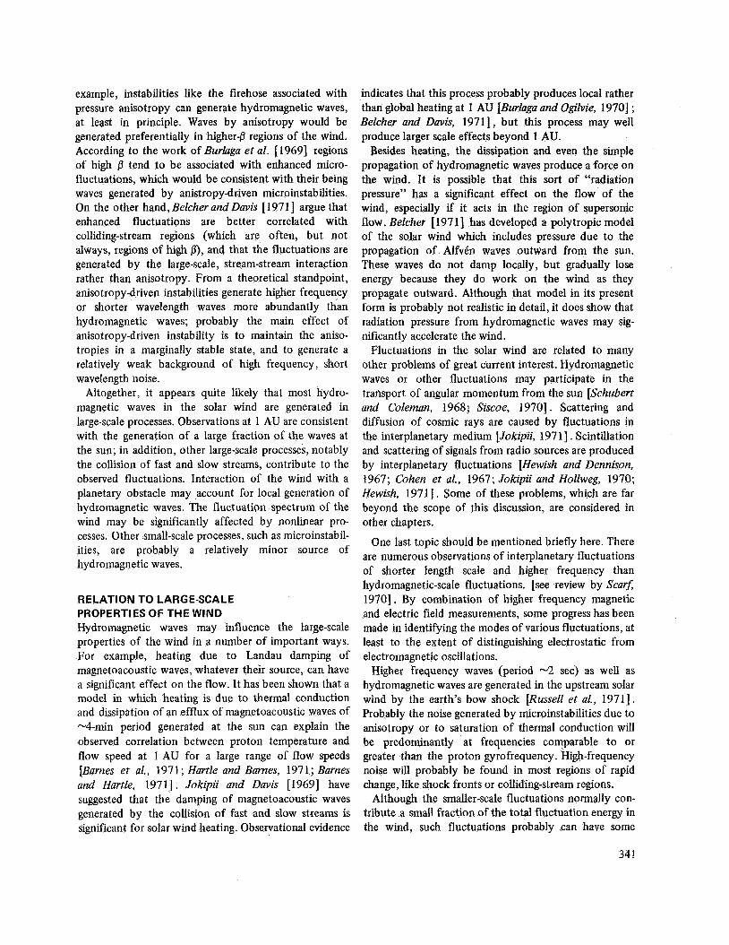
4 Figure 3. Marginal stability curve for the electrostatic ion cyclotron wave as a function of fl for Te/Ti= 1 and contours of maximum growth rate of the electromug- netic ion cyclotron wave versus fl for Te/Ti= 1; VD is the electron drift velocity or net shift in the electron peak from that of the ions; a, is the electron thermal velocity.

neighborhood of = 0.01 it starts to rise more sharply. Figure 3 also shows the maximum growth rate contours of the electromagnetic ion-cyclotron wave obtained by numerically searching the full hot plasma electromagnetic dispersion relation. Note that these contours drop to very low drifts as 0 increases; 0 - 0.01 is probably typical when close to the critical radius and analytically depends exactly on what kind of model is used. At any rate, near 10 R , the electromagnetic ion-cyclotron mode may indeed be unstable along with the ion-acoustic wave and cause modification of the transport coefficients. These results need to be extended to 0 = 1 to determine more carefully what happens as one approaches the orbit of earth.

Thus we see that there are a moderate number of instabilities that can take place due to heat conduction. With the exception of the ion-acoustic mode, the most unstable modes have wavelengths about that of the ion gyroradius, although most of the instabilities can grow at very long wavelength but at reduced rates of growth. What sort of turbulence they produce is uncertain, but one would expect a peak at around the ion gyroradius.

I would next like to discuss the instabilities that can occur from the proton and electron anisotropy created by the nearly adiabatic expansion of the plasma out from the sun. It is known that a very large anisotropy, Tl<<TII, should develop which in turn should destabilize Alfvkn waves, thus reducing the anisotropy, more closely approaching the values found in the solar wind. We have recently looked at finite gyroradius effects on these instabilities more carefully, both analytically and numerically and by searching the electromagnetic dispersion relation over a range of wave numbers kll, propagation angles, anisotropies, and 0, and by studying the maximum growth rates. We have uncovered several interesting effects. [Kennel and Scar- 19681 discussed the case for waves propagating exactly along the field lines, but we have recently looked at the oblique firehose instability, which has zero real frequency at large angles to B and continues to have zero frequency as one approaches finite gyroradius. For Tl<<TII and zero real frequency, the condition for marginal stability

349

is found where P+ is the proton pressure along the field relative to the magnetic pressure, A+ is the proton anisotropy l-Tl/Tll, RL,, is the proton gyroradius, andZ ' i s the plasma-dispersion function, involving only parallel wave numbers. The electron aniso- tropy enters in the usual firehose fashion. In the asymptotic long wavelength limit the coefficient of P+A+-+l, giving the usual criterion for firehose instability. However, for finite gyroradius, this coefficient has a maximum of 1.65, thus reducing the anisotropies and 0, which can give rise to instability. As will be shown later, this may be significant. For the parallel whistler mode one can also show that this occurs at finite gyroradius, as indicated by Kennel and Scarf [1968] and also more recently by Hollweg and Vdlk [I9701 . In particular, one can derive an expression from Kennel and Scarf if the anisotropy A?@. 1)

Here the left-hand side of the expression is the normal firehose criterion. The finite gyroradius effect destabilizes the firehose-that is, permits it to function for parameter values below the hydromagnetic firehose Iimit. Since both modes have lower thresholds at finite gyroradius, the nonlinear evolution will stabilize these waves and reduce the anisotropy before the hydromagnetic limit is reached. Thus, in the firehose case, it appears that the short wavelength turbulence is very important.

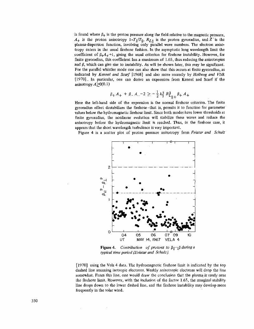
Figure 4 is a scatter plot of proton pressure anisotropy from Eviatar and Schulz

2

ai Q I

a- Q -

I

" 04 05 06 07"09 IO

UT MAY 14, 1967 VELA 4

Figure 4. Contribution of protons to PlI-l/3 during a typical time period (Eviatar and Schulz).

[1970] using the Vela 4 data. The hydromagnetic firehose limit is indicated by the top dashed line assuming isotropic electrons. Weakly anisotropic electrons will drop the line somewhat. From this line, one would draw the conclusion that the plasma is rarely near the firehose limit. However, with the inclusion of the factor 1.65, the marginal stability line drops down to the lower dashed line, and the firehose instability may develop more frequently in the solar wind.

350

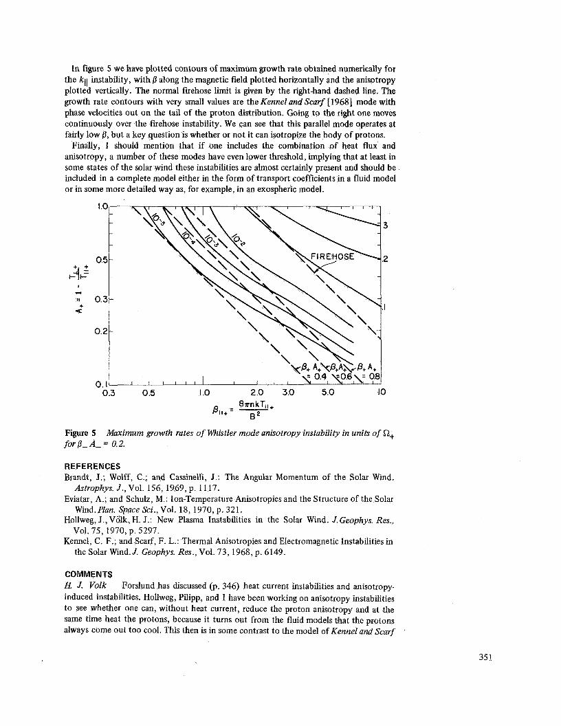
In figure 5 we have plotted contours of maximum growth rate obtained numerically for the kll instability, with 0 along the magnetic field plotted horizontally and the anisotropy plotted vertically. The normal firehose limit is given by the right-hand dashed line. The growth rate contours with very small values are the Kennel and Scarf [ 19681 mode with phase velocities out on the tail of the proton distribution. Going to the right one moves continuously over the firehose instability. We can see that this parallel mode operates at fairly low 0, but a key question is whether or not it can isotropize the body of protons.

Finally, I should mention that if one includes the combination of heat flux and anisotropy, a number of these modes have even lower threshold, implying that at least in some states of the solar wind these instabilities are almost certainly present and should be included in a complete model either in the form of transport coefficients in a fluid model or in some more detailed way as, for example, in an exospheric model.

I .o 3

0.5 .2 + + $12

I .c1

1: 0.3 + .I a

0.2

0. I 0.3 0.5 I .o 2.0 3.0 5.0 IO

87rn k T, , +

PI,+= 7 Figure 5 for 0- A- = 0.2.

Maximum growth rates of Whistler mode anisotropy instability in units of s1,

REFERENCES Brandt, J.; Wolff, C. ; and Cassinelli, J.: The Angular Momentum of the Solar Wind.

Eviatar, A.; and Schulz, M.: Ion-Temperature Anisotropies and the Structure of the Solar

Hollweg, J., Volk, H. J.: New Plasma Instabilities in the Solar Wind. J. Geophys. Res.,

Kennel, C. F.; and Scarf, F. L.: Thermal Anisotropies and Electromagnetic Instabilities in

Astrophys. J., Vol. 156, 1969, p. 1117.

Wind. Plan. Space Sci., Vol. 18, 1970, p. 321.

Vol. 75, 1970, p. 5297.

the Solar Wind. J. Geophys. Res., Vol. 73, 1968, p. 6 149.

COMMENTS I3 J. Volk Forslund has discussed (p. 346) heat current instabilities and anisotropy- induced instabilities. Hollweg, Pilipp, and I have been working on anisotropy instabilities to see whether one can, without heat current, reduce the proton anisotropy and at the same time heat the protons, because it turns out from the fluid models that the protons always come out too cool. This then is in some contrast to the model of Kennel and Scarf

who used, as we do, parallel propagating hydromagnetic waves. Because in their model-although this is the most likely candidate to reduce the proton anisotropy-at the same time the protons are cooled, and this is not in line with the two-fluid model. So we include an electron anisotropy and try to see whether the electrons, which are hot and anisotropic, can both lower the anisotropy and heat the protons.

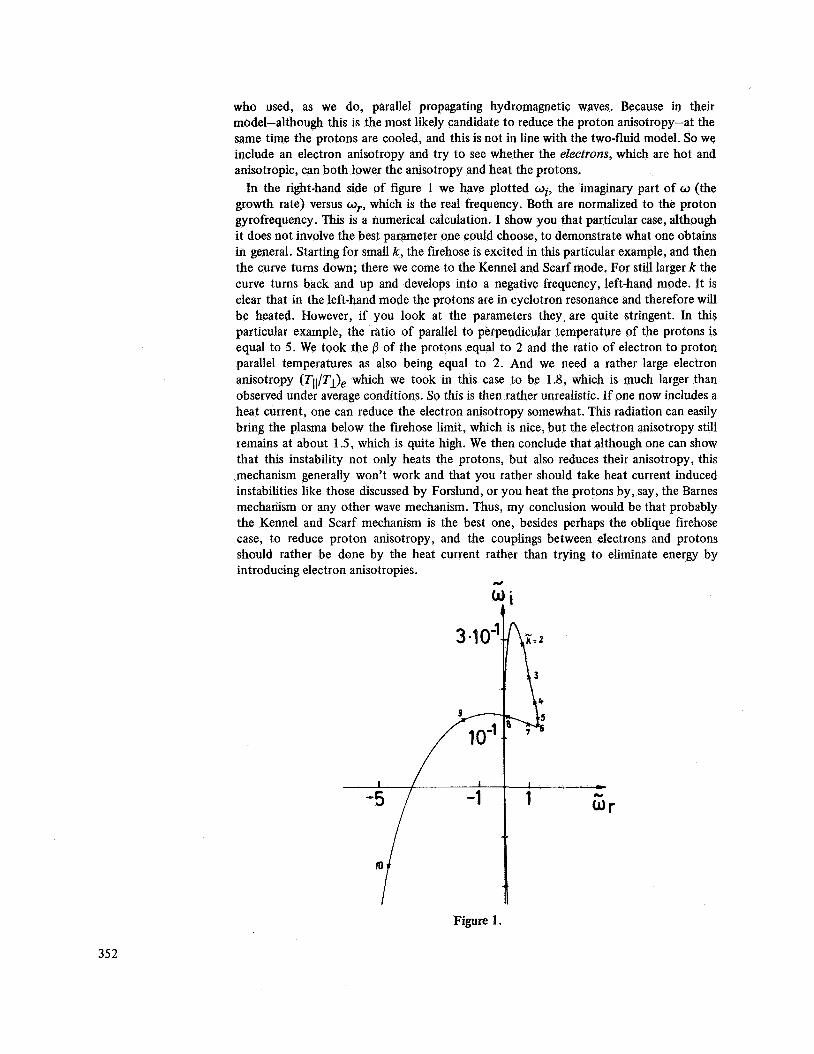
In the right-hand side of figure 1 we have plotted wi, the imaginary part of w (the growth rate) versus a,., which is the real frequency. Both are normalized to the proton gyrofrequency. This is a numerical calculation. I show you that particular case, although it does not involve the best parameter one could choose, to demonstrate what one obtains in general. Starting for small k , the firehose is excited in this particular example, and then the curve turns down; there we come to the Kennel and Scarf mode. For still larger k the curve turns back and up and develops into a negative frequency, left-hand mode. It is clear that in the left-hand mode the protons are in cyclotron resonance and therefore will be heated. However, if you look at the parameters they.are quite stringent. In this particular example, the ratio of parallel to perpendicular temperature of the protons is equal to 5. We took the 0 of the protons equal to 2 and the ratio of electron to proton parallel temperatures as also being equal to 2. And we need a rather large electron anisotropy (Tll/Tl)e which we took in this case to be 1.8, which is much larger than observed under average conditions. So this is then rather unrealistic. If one now includes a heat current, one can reduce the electron anisotropy somewhat. This radiation can easily bring the plasma below the firehose limit, which is nice, but the electron anisotropy still remains at about 1.5, which is quite high. We then conclude that although one can show that this instability not only heats the protons, but also reduces their anisotropy, this mechanism generally won't work and that you rather should take heat current induced instabilities like those discussed by Forslund, or you heat the protons by, say, the Barnes mechafiism or any other wave mechanism. Thus, my conclusion would be that probably the Kennel and Scarf mechanism is the best one, besides perhaps the oblique firehose case, to reduce proton anisotropy, and the couplings between electrons and protons should rather be done by the heat current rather than trying to eliminate energy by introducing electron anisotropies.

&

Figure 1.

352