Embed Size (px)
Citation preview
Final Report
The Social and Economic Impact of South Africa’s Social Security System
30 September 2004
Commissioned by the Directorate: Finance and Economics
Produced by the Economic Policy Research Institute
Dr. Michael Samson Ms. Una Lee
Mr. Asanda Ndlebe Mr. Kenneth Mac Quene Ms. Ingrid van Niekerk
Mr. Viral Gandhi Ms. Tomoko Harigaya Ms. Celeste Abrahams
Economic Policy Research InstituteA SECTION 21 COMPANY · Reg. number 1998/09814/08
SANCLARE BUILDING 3rd FLOOR 21 DREYER STREET CLAREMONT 7700 CAPE TOWN TEL: (+27 21) 671-3301 www.epri.org.za FAX: (+27 21) 671-3157
Board of Directors Ms. Fikile Soko-Masondo, Ms. Ingrid van Niekerk, Mr. Kenneth Mac Quene, Dr. Michael J. Samson, Mr. Robert van Niekerk, Ms. Tholi Nkambule, Mr. Zunaid Moolla
Department of Social Development
1
Final Report Executive Summary
The Social and Economic Impact of South Africa’s Social Security System
Commissioned by the Economics and Finance Directorate, Dept. of Social Development
Produced by the Economic Policy Research Institute
Dr. Michael Samson Ms. Una Lee
Mr. Asanda Ndlebe Mr. Kenneth Mac Quene Ms. Ingrid van Niekerk
Mr. Viral Gandhi Ms. Tomoko Harigaya Ms. Celeste Abrahams
30 September 2004
Social grants in South Africa play a critical role in reducing poverty and promoting social development. This study evaluates the social and economic impact of State Old Age Pensions (SOAP), Disability Grants (DG), Child Support Grants (CSG), Care Dependency Grants (CDG), Foster Care Grants (FCG) and Grants-in-Aid (GIA). The analysis evaluates the role of social assistance in reducing poverty and promoting household development, examining effects on health, education, housing and vital services. In addition, the study assesses the impact of social grants on labour market participation and labour productivity, providing an analysis of both the supply and demand sides of the labour market. The study also quantifies the macro-economic impact of social assistance grants, evaluating their impact on savings, consumption and the composition of aggregate demand. Most of the statistical analysis focuses on the CSG, SOAP and DG since sample sizes are sufficiently large for these grants to support significant inferences. South Africa’s system of social security successfully reduces poverty, regardless of which methodology is used to quantify the impact measure or identify the poverty line. Nevertheless, the quantitative measure of poverty reduction is sensitive to the methodological choices. For instance, the measured impact is consistently greatest when employing the total rand poverty gap as an indicator. The poverty headcount measure, however, consistently yields the smallest results. Likewise, the choice of poverty line heavily influences the measurement of the quantitative impact. The currently social security system is most successful when measured against destitution, and the impact is smallest when poverty lines ignore economies of scale and adult equivalence issues. For instance, South Africa’s social grants reduce the poverty headcount measure by 4.3%, as measured against the Committee of Inquiry’s expenditure poverty line (with no scales). The social security system, however, reduces 45% of the total rand destitution gap—an impact more than ten times greater. Using the Committee of Inquiry expenditure poverty line (without scales), a 10% increase in take-up of the SOAP reduces the poverty gap by only 1.2%, and full take-up by only 2.5%. The take-up rate for the SOAP is already very high, and many of the eligible elderly not already receiving the SOAP are not among the poorest South Africans. As a result, further extensions of the SOAP have limited potential in reducing poverty. Extensions of the Disability Grant offer greater promise, although at substantially greater expense. A 50% increase in DG take-up reduces the total rand poverty gap by 1.7%, and full take-up generates a 5.1% reduction. The greatest poverty reducing potential lies with the
2
progressive extension of the Child Support Grant. Extending the eligibility age to 14 reduces the poverty gap by 16.6%, and a further extension to age 18 reduces the gap by 21.4%. Increasing the real grant payment (as the government did in 2003) generates an even greater impact. The extension to age 14 yields a 22% poverty gap reduction, while the extension to age 18 reduces the poverty gap by 28.3%. Combining the higher CSG extended to age 14 with the full take-up of the SOAP and the DG yields a reduction in the total rand poverty gap of 29%. The magnitudes of these effects, of course, depend critically on the poverty line by which the impacts of the reforms are measured. For instance, the 29% reduction in the total rand poverty gap measured using the unscaled Committee of Inquiry expenditure poverty line is less than half the magnitude of the reduction in destitution, which amounts to a 66.6% reduction. Likewise, the impacts of the scaled Committee of Inquiry income and expenditure poverty lines are substantially greater than for the unscaled poverty lines. The impact of the “all grants” package measured with the scaled Committee of Inquiry income poverty line reflects a 47.4% reduction, and with the expenditure poverty line, a comparable 47.5% reduction. As this makes apparent, the distinction between income and expenditure poverty has not generated material differences in this analysis. Likewise, the impact using the unscaled Committee of Inquiry income poverty line (a 28.9% reduction) is virtually the same as that using the unscaled Committee of Inquiry expenditure poverty line (a 29.0% reduction). For almost every simulation, the HSL poverty line generates very close results to those yielded by the scaled Committee of Inquiry income and expenditure poverty lines, in spite of the substantial methodological differences distinguishing the HSL measure. The relative poverty line yields results that are not closely comparable to any of the other poverty line measures, with the results generally falling in between the results of the Committee of Inquiry scaled and unscaled poverty line measures. The evidence in this report documents the substantial impact of South Africa’s social security system in reducing poverty and destitution. The magnitudes of the results are sensitive to methodological issues. It matters whether the poverty line is relative or absolute, whether it is scaled for household composition and economies of scale or not, and to a small extent whether it measures income or expenditure. Likewise, it matters how the poverty impact is measured—using poverty headcount or variants on the poverty gap. Nevertheless, the qualitative results, and the answers to critical policy questions, are robust to different methodological approaches. South Africa’s system of social security substantially reduces deprivation, and the progressive extension of the magnitude, scope and reach of social grants holds the potential to dramatically diminish the prevalence of poverty in South Africa. The results of this study provide evidence that the household impacts of South Africa’s social grants are developmental in nature. These findings are consistent with international lessons of experience, as well as with previous studies of South Africa’s system of social security. Social security programmes in Brazil, Argentina, Namibia and Botswana yield positive impacts in terms of reducing poverty, promoting job search and increasing school attendance. Past studies of social security in South Africa have focused on the State Old Age Pension, identifying important positive effects in terms of broadly reducing household poverty as well as improving health and nutrition. Poverty and its associated consequences erode the opportunities for children and youth to attend school, fomenting a vicious cycle of destitution by undermining the household’s capacity to accumulate the human capital necessary to break the poverty trap. The statistical evidence from this research documents the extent to which poverty exerts a negative impact on school enrolment rates. Many poor children cannot attend school due to the costs associated with education, including the necessity to work to supplement family income. In
3
addition, communities that are resource-constrained provide lower quality educational services, which negatively affects enrolment rates. Social security grants counter these negative effects by providing households with more resources to finance education. New findings from this study demonstrate that children in households that receive social grants are more likely to attend school, even when controlling for the effect of income. The positive effects of social security on education are greater for girls than for boys, helping to remedy gender disparities. But both the State Old Age Pension and the Child Support Grant are statistically significantly associated with improvements in school attendance, and the magnitudes of these impacts are substantial. This analysis only measures the direct and static link between social security and education. To the extent that social grants promote school attendance, they contribute to a virtuous cycle with long term dynamic benefits that are not easily measured by statistical analysis. Nationally, nearly one in five households experienced hunger during the year studied (2000). The highest income provinces—Gauteng and the Western Cape—have the lowest prevalence rates of hunger. The prevalence rate of hunger is highest in one of South Africa’s poorest provinces—nearly one in three households in the Eastern Cape experiences hunger. However, another of the poorest provinces—Limpopo—has the third lowest hunger prevalence rate in the country. Meanwhile, Mpumalanga—with a poverty rate below the national average—has the second highest hunger prevalence rate in the country. Social grants are effective in addressing this problem of hunger, as well as basic needs in general. Spending in households that receive social grants focuses more on basics like food, fuel, housing and household operations, and less is spent on tobacco and debt. All major social grants—the State Old Age Pension, the Child Support Grant and the Disability Grant—are significantly and positively associated with a greater share of household expenditure on food. This increased spending on food is associated with better nutritional outcomes. Households that receive social grants have lower prevalence rates of hunger for young children as well as older children and adults, even compared to those households with comparable income levels. Receipt of social grants is associated with lower spending on health care, perhaps because social grants are associated with other positive outcomes that reduce the need for medical care. For instance, the World Bank identifies the important link between improved education and stemming the spread of HIV/AIDS. Likewise, social grants are associated with greater household access to piped water. The evidence in this chapter underscores the importance of moving beyond measures of income poverty in the assessment of social deprivation. In case after case in this study, household outcomes conflicted with the simple implications of monetary income rankings. While many measures of well-being are correlated with aggregate income and expenditure, the exceptions affect large numbers of people and require careful policy analysis. The interaction between social security and household well-being is complex, and further research continues to explore these interactions. In particular, the broad measures of household well-being analysed in this chapter exert profound effects on labour productivity and the ability of workers to find jobs. Employment in turn provides access to resources that promote improved education, nutrition, health and other outcomes. Conventional economic theory suggests that social grants may undermine labour force participation by reducing the opportunity cost of not working. Models developed for industrialised countries and applied broadly to South African data sometimes corroborate this hypothesis. However, when models are developed that reflect the labour market behaviour of South Africans who receive social grants, the results contradict this hypothesis. The response of very low income South Africans to a marginal increase in their income is significantly different from the response of median income South Africans.
4
To the extent that social grants create adverse labour market effects, the adverse consequences stem from distortions in social security targeting mechanisms. For instance, to the extent that the State Old Age Pensions are employed to target the non-pensioner poor, then the grants may encourage a household formation response that impedes job search. These types of problems can be addressed by broadening the base of the social security programmes. The more comprehensive the system of social security, the fewer distortions are generated by the incentive effects created by the social grants. This study explicitly examines the impact of social grants on the labour market participation, employment success and realised wages of South Africans in households receiving social grants. While statistical analysis cannot prove causation, the empirical results are consistent with the hypotheses that: (1) Social grants provide potential labour market participants with the resources and economic security necessary to invest in high-risk/high-reward job search. (2) Living in a household receiving social grants is correlated with a higher success rate in finding employment. (3) Workers in households receiving social grants are better able to improve their productivity and as a result earn higher wage increases. The empirical evidence discussed in this chapter demonstrates that people in households receiving social grants have increased both their labour force participation and employment rates faster than those who live in households that do not receive social grants. In addition, workers in households receiving social grants have realised more rapid wage increases. These findings are consistent with the hypothesis that South Africa’s social grants increase both the supply and demand for labour. This evidence does not support the hypothesis that South Africa’s system of social grants negatively affects employment creation. At the macro-economic level, South Africa’s system of social development grants tends to increase domestic employment while promoting a more equal distribution of income. The effects of grants on national savings and the trade balance are ambiguous, since grants have two competing effects on the national savings—one through private domestic savings, and the other through the trade deficit. Depending on the magnitude of the effects, grants could improve or worsen national savings and the trade balance. Initial analysis suggests that the impact on savings may be negative, while that on the trade balance may be positive. However, since much of the savings of upper income groups are offshore, the negative impact is unlikely to be significant, particularly given the small share of private savings in the national savings rate. The impact on inflation may also be ambiguous. The increase in overall demand in the economy may generate some inflationary pressure. However, the relatively low rate of capacity utilisation may enable the economy to meet this demand without significant increases in inflation. Likewise, the positive trade balance effects may lead to an appreciation of the rand, tending to dampen imported inflation. On balance, the macro-economic impact of South Africa’s social security system is largely positive. These positive macroeconomic effects support higher rates of economic growth, which are re-inforced by the social security system’s positive effects on income distribution and education.
5
TABLE OF CONTENTS Executive Summary 1 Chapter 1: Introduction 13
Chapter 2: The Impact of Social Assistance on Poverty Reduction 15 2.1 Introduction 15 2.2 Methodology 16 2.3 The EPRI Micro-Simulation Model 25 2.4 The Impact of South Africa’s Social Security System 29 2.5 Simulations of South Africa’s Social Security Reform Options 33 2.6 Summary and conclusions 52 Chapter 3: The Household Impact of Social Assistance Programmes 55 3.1 Introduction 55 3.2 Background and Literature Review 55 3.3 Social Security and Education 60 3.4 The Household Spending Impact of Social Security 73 3.5 Social Security and Nutrition 78 3.6 Social Security and Health 82 3.7 Other Social Indicators 84 3.8 Conclusions 85 Chapter 4: The Labour Market Impact of Social Assistance Programmes 87 4.1 Introduction 87 4.2 Literature Review 87 4.3 Social Security and Labour Supply 91 4.4 Labour Demand 112 4.5 Policy Implications 117 Chapter 5: The Macro-economic Impact of Social Assistance Programmes 119 5.1 Introduction 119 5.2 Composition of Spending 119 5.3 Savings, Investment, and the Balance of Trade 123 5.4 Impact of Social Grants on Inflation 125 5.5 Macro-economic Impact of Social Grants from Inequality Reduction 127 5.6 Macro-economic Impact of Social Grants through Education 130 5.7 Conclusion 132 Chapter 6: Summary, Conclusions and Policy Implications 133 6.1 The impact on poverty 133 6.2 The impact on household well-being 134 6.3 The labour market impact 134 6.4 The macro-economic impact 134
6
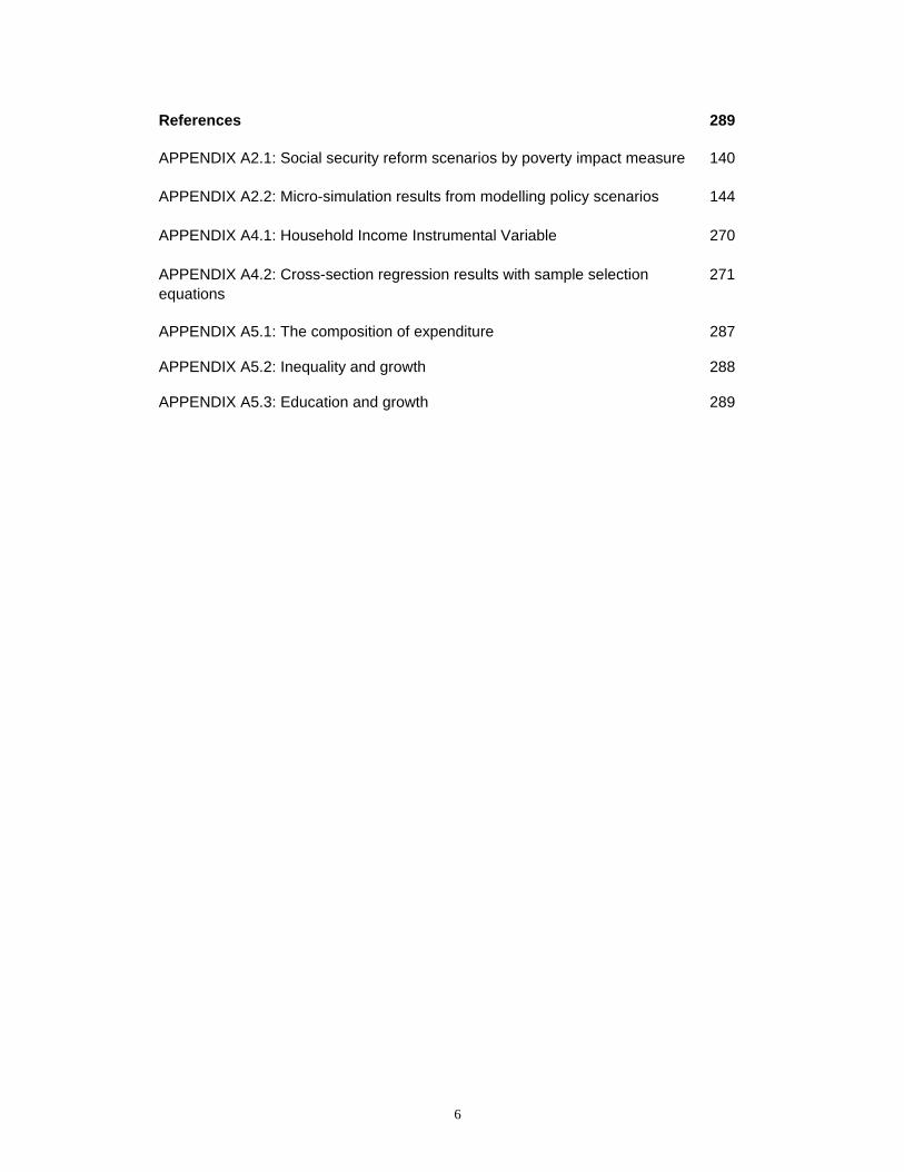
References 289 APPENDIX A2.1: Social security reform scenarios by poverty impact measure 140 APPENDIX A2.2: Micro-simulation results from modelling policy scenarios 144 APPENDIX A4.1: Household Income Instrumental Variable 270 APPENDIX A4.2: Cross-section regression results with sample selection 271 equations APPENDIX A5.1: The composition of expenditure 287 APPENDIX A5.2: Inequality and growth 288 APPENDIX A5.3: Education and growth 289
7
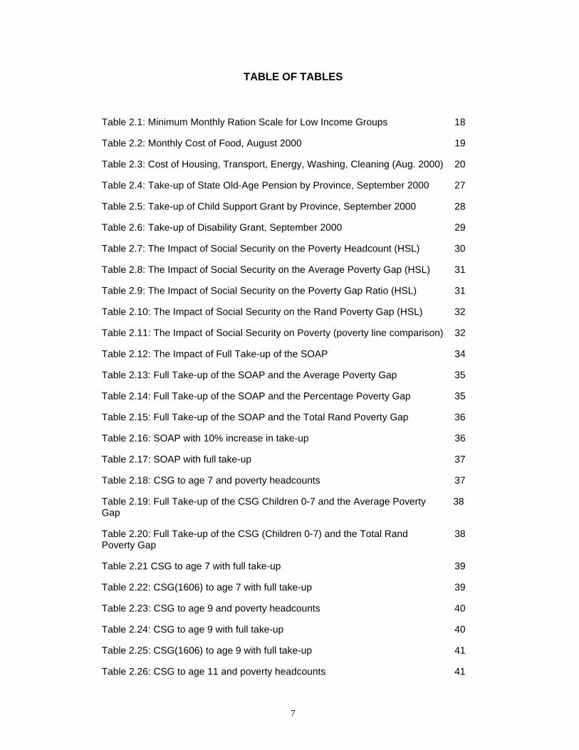
TABLE OF TABLES
Table 2.1: Minimum Monthly Ration Scale for Low Income Groups 18
Table 2.2: Monthly Cost of Food, August 2000 19
Table 2.3: Cost of Housing, Transport, Energy, Washing, Cleaning (Aug. 2000) 20
Table 2.4: Take-up of State Old-Age Pension by Province, September 2000 27
Table 2.5: Take-up of Child Support Grant by Province, September 2000 28
Table 2.6: Take-up of Disability Grant, September 2000 29
Table 2.7: The Impact of Social Security on the Poverty Headcount (HSL) 30
Table 2.8: The Impact of Social Security on the Average Poverty Gap (HSL) 31
Table 2.9: The Impact of Social Security on the Poverty Gap Ratio (HSL) 31
Table 2.10: The Impact of Social Security on the Rand Poverty Gap (HSL) 32
Table 2.11: The Impact of Social Security on Poverty (poverty line comparison) 32
Table 2.12: The Impact of Full Take-up of the SOAP 34
Table 2.13: Full Take-up of the SOAP and the Average Poverty Gap 35
Table 2.14: Full Take-up of the SOAP and the Percentage Poverty Gap 35
Table 2.15: Full Take-up of the SOAP and the Total Rand Poverty Gap 36
Table 2.16: SOAP with 10% increase in take-up 36
Table 2.17: SOAP with full take-up 37
Table 2.18: CSG to age 7 and poverty headcounts 37
Table 2.19: Full Take-up of the CSG Children 0-7 and the Average Poverty 38 Gap
Table 2.20: Full Take-up of the CSG (Children 0-7) and the Total Rand 38 Poverty Gap
Table 2.21 CSG to age 7 with full take-up 39
Table 2.22: CSG(1606) to age 7 with full take-up 39
Table 2.23: CSG to age 9 and poverty headcounts 40
Table 2.24: CSG to age 9 with full take-up 40
Table 2.25: CSG(1606) to age 9 with full take-up 41
Table 2.26: CSG to age 11 and poverty headcounts 41
8
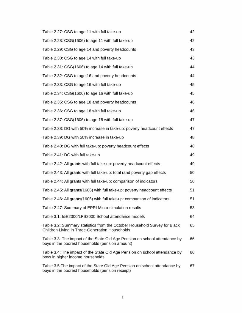
Table 2.27: CSG to age 11 with full take-up 42
Table 2.28: CSG(1606) to age 11 with full take-up 42
Table 2.29: CSG to age 14 and poverty headcounts 43
Table 2.30: CSG to age 14 with full take-up 43
Table 2.31: CSG(1606) to age 14 with full take-up 44
Table 2.32: CSG to age 16 and poverty headcounts 44
Table 2.33: CSG to age 16 with full take-up 45
Table 2.34: CSG(1606) to age 16 with full take-up 45
Table 2.35: CSG to age 18 and poverty headcounts 46
Table 2.36: CSG to age 18 with full take-up 46
Table 2.37: CSG(1606) to age 18 with full take-up 47
Table 2.38: DG with 50% increase in take-up: poverty headcount effects 47
Table 2.39: DG with 50% increase in take-up 48
Table 2.40: DG with full take-up: poverty headcount effects 48
Table 2.41: DG with full take-up 49
Table 2.42: All grants with full take-up: poverty headcount effects 49
Table 2.43: All grants with full take-up: total rand poverty gap effects 50
Table 2.44: All grants with full take-up: comparison of indicators 50
Table 2.45: All grants(1606) with full take-up: poverty headcount effects 51
Table 2.46: All grants(1606) with full take-up: comparison of indicators 51
Table 2.47: Summary of EPRI Micro-simulation results 53
Table 3.1: I&E2000/LFS2000 School attendance models 64
Table 3.2: Summary statistics from the October Household Survey for Black 65 Children Living in Three-Generation Households
Table 3.3: The impact of the State Old Age Pension on school attendance by 66 boys in the poorest households (pension amount)
Table 3.4: The impact of the State Old Age Pension on school attendance by 66 boys in higher income households
Table 3.5:The impact of the State Old Age Pension on school attendance by 67 boys in the poorest households (pension receipt)
9
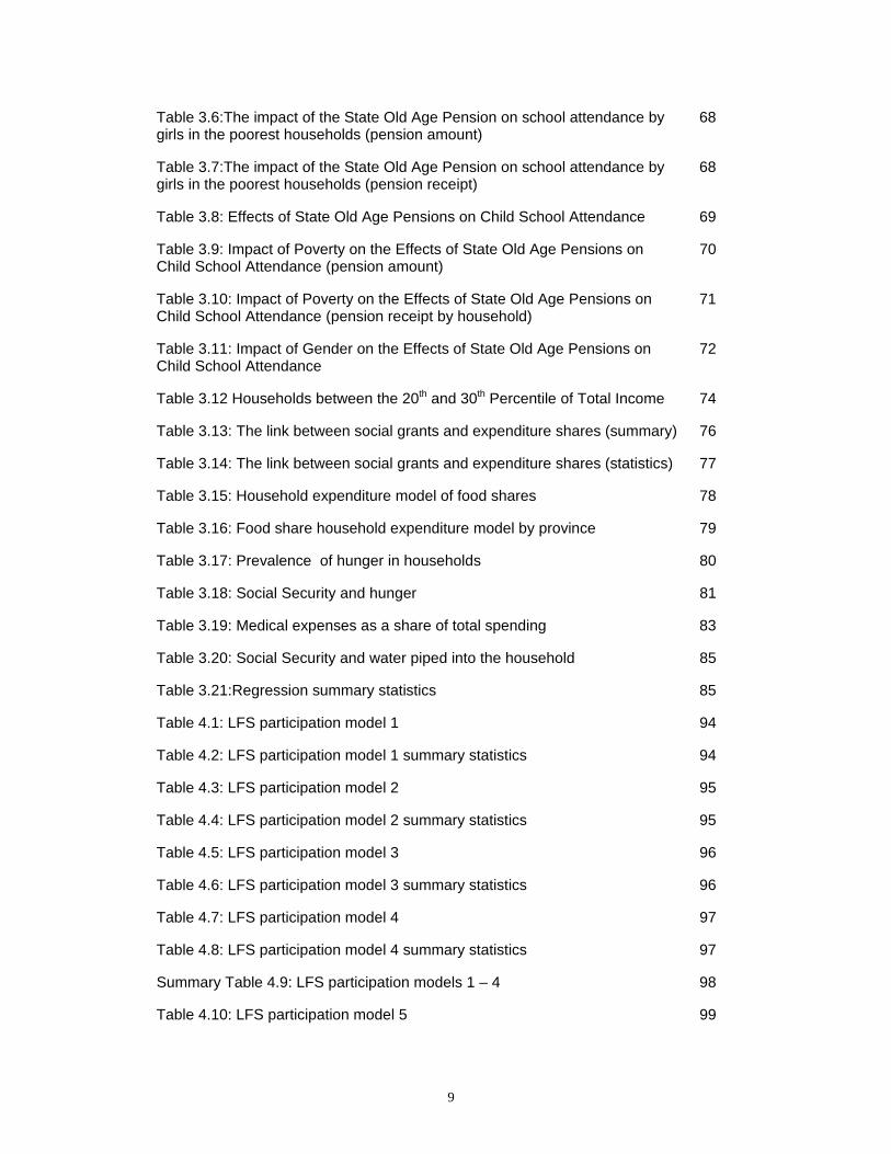
Table 3.6:The impact of the State Old Age Pension on school attendance by 68 girls in the poorest households (pension amount)
Table 3.7:The impact of the State Old Age Pension on school attendance by 68 girls in the poorest households (pension receipt)
Table 3.8: Effects of State Old Age Pensions on Child School Attendance 69
Table 3.9: Impact of Poverty on the Effects of State Old Age Pensions on 70 Child School Attendance (pension amount)
Table 3.10: Impact of Poverty on the Effects of State Old Age Pensions on 71 Child School Attendance (pension receipt by household)
Table 3.11: Impact of Gender on the Effects of State Old Age Pensions on 72 Child School Attendance
Table 3.12 Households between the 20th and 30th Percentile of Total Income 74
Table 3.13: The link between social grants and expenditure shares (summary) 76
Table 3.14: The link between social grants and expenditure shares (statistics) 77
Table 3.15: Household expenditure model of food shares 78
Table 3.16: Food share household expenditure model by province 79
Table 3.17: Prevalence of hunger in households 80
Table 3.18: Social Security and hunger 81
Table 3.19: Medical expenses as a share of total spending 83
Table 3.20: Social Security and water piped into the household 85
Table 3.21:Regression summary statistics 85
Table 4.1: LFS participation model 1 94
Table 4.2: LFS participation model 1 summary statistics 94
Table 4.3: LFS participation model 2 95
Table 4.4: LFS participation model 2 summary statistics 95
Table 4.5: LFS participation model 3 96
Table 4.6: LFS participation model 3 summary statistics 96
Table 4.7: LFS participation model 4 97
Table 4.8: LFS participation model 4 summary statistics 97
Summary Table 4.9: LFS participation models 1 – 4 98
Table 4.10: LFS participation model 5 99
10
Table 4.11: LFS participation model 5 summary statistics 99
Table 4.12: LFS participation model 6 100
Table 4.13: LFS participation model 6 summary statistics 100
Table 4.14: LFS participation model 7 101
Table 4.15: LFS participation model 7 summary statistics 101
Table 4.16: LFS participation model 8 102
Table 4.17: LFS participation model 8 summary statistics 102
Summary Table 4.18: LFS participation models 5 – 8 103
Table 4.19: LFS employment model 1 104
Table 4.20: LFS employment model 1 summary statistics 104
Table 4.21: LFS employment model 2 104
Table 4.22: LFS employment model 2 summary statistics 105
Table 4.23: LFS employment model 3 105
Table 4.24: LFS employment model 3 summary statistics 105
Table 4.25: LFS employment model 4 106
Table 4.26: LFS employment model 4 summary statistics 106
Summary Table 4.27: LFS employment models 1 – 4 107
Table 4.28: LFS employment model 5 107
Table 4.29: LFS employment model 5 summary statistics 108
Table 4.30: LFS employment model 6 108
Table 4.31: LFS employment model 6 summary statistics 109
Table 4.32: LFS employment model 7 109
Table 4.33: LFS employment model 7 summary statistics 109
Table 4.34: LFS employment model 8 110
Table 4.35: LFS employment model 8 summary statistics 110
Summary Table 4.36: LFS employment models 5 – 8 111
Table 4.37: Wages and social grants 113
Table 4.38: LFS wage model 1 114
Table 4.39: LFS wage model 1 summary statistics 114
11
Table 4.40: LFS wage model 2 115
Table 4.41: LFS wage model 2 summary statistics 115
Table 4.42: LFS wage model 3 116
Table 4.43: LFS wage model 3 summary statistics 116
Summary Table 4.44: LFS wage models 1 – 3 117
Table 5.1: Expenditure Shares by Income Deciles 119
Table 5.2: Analysis of spending categories (based on 1st Quarter 2002 data) 122
Table 5.3: Balance of Trade Analysis 125
Table 5.4: Capacity Utilisation by Sector 126
Table 5.5: The Barro model of economic growth 131
Table 5.6: The Gylfason model of economic growth 131
APPENDIX A2.1: Social security reform scenarios by poverty impact measure 140 (Table A2.1.1 – tableA2.1.7)
APPENDIX A2.2: Micro-simulation results from modelling policy scenarios 144 (Table A2.2.1- Table A2.2.126)
APPENDIX A4.1: Household Income Instrumental Variable 270
APPENDIX A4.2: Cross-section regression results with sample selection 271 equations (Table A4.2.1 - Table A4.2.24)
APPENDIX A5.1: The composition of expenditure (Table A5.1.1) 287
APPENDIX A5.2: Inequality and growth (Table A5.2.1) 288
APPENDIX A5.3: Education and growth (Table A5.3.1) 289
12
TABLE OF FIGURES Figure 5.1: Food expenditure share of household spending by income group 120
Figure 5.2: Transportation share of household spending by income group 121
Figure 5.3: Clothing share of household spending by income group 121
Figure 5.4: Savings rates by income group 123
Figure 5.5: Debt as a percentage of total household income, by income group 124
Figure 5.6: Manufacturing capacity utilisation: durable versus non-durable 126
Figure 5.7: Initial inequality and subsequent economic growth 128
Figure 5.8: The impact of social grants on South Africa’s distribution of income 129
Figure 5.9: The relationship between education and growth 132
13
CHAPTER 1) Introduction
South Africa’s social grants play a vital role in reducing poverty and promoting social development. Numerous academic studies document the broad social and economic impact of these effective social security programmes. This report provides an appraisal of the impact of State Old Age Pensions (SOAP), Disability Grants (DG), Child Support Grants (CSG), Care Dependency Grants (CDG), Foster Care Grants (FCG) and Grants-in-Aid (GIA). The analysis evaluates the role of social assistance in reducing poverty and promoting household development, examining effects on health, education, housing and vital services. In addition, the study assesses the impact of social grants on labour market participation and labour productivity, providing an analysis of both the supply and demand sides of the labour market. The study also quantifies the macro-economic impact of social assistance grants, evaluating their impact on savings, consumption and the composition of aggregate demand.
This paper is divided into four major chapters. The first major chapter (chapter 2) employs EPRI’s micro-simulation model calibrated with administrative data for January 2003. The model, using Statistic South Africa’s Labour Force Survey and 2000 Income and Expenditure Survey, provides measures of social assistance take-up by household income level. In addition, the surveys provide detailed profiles on the household’s living standards, labour market activity and consumption patterns. This chapter assesses the impact of the current system of social grants on poverty reduction. In addition, alternative scenarios of social security reform are evaluated and compared, with a particular focus on extensions of the Child Support Grant. The study analyses the impact of methodological issues on poverty analysis.
The second major chapter (chapter 3) uses this model to evaluate how receipt of social assistance grants affects household access to health care, schooling, housing, electricity, water and social infrastructure. The chapter analyses survey data provided by Statistics South Africa, building models of household expenditure and testing how receipt of social grants affects spending patterns. In addition, the study investigates direct outcomes variables, such as school attendance, and how these are affected by the receipt of social grants by households.
The third major chapter (chapter 4) extends this household analysis to the labour market, examining the impact of social grants on employment and productivity The chapter analyses Statistics South Africa’s Labour Force Survey, evaluating the impact of social grants on labour force participation and employment success. The study also evaluates the impact of social grants on realised wages, as a measure of the impact of social grants on labour force productivity. The analysis includes both cross-section and panel data econometric models, as well as descriptive statistics.
The fourth major chapter (chapter 5) analyses the macro-economic impact, aggregating the micro-simulation variables to calculate effects on national savings and
14
consumption by economic sector. In addition, this chapter evaluates macro-economic data provided by Statistics South Africa, the Reserve Bank of South Africa and the National Treasury. This chapter builds on the household impact analysis from chapter 3, extending these findings to the macro-economic level.
The final chapter (chapter 6) summarises the key findings of the study and briefly discusses the conclusions and policy implications.
15
CHAPTER 2) The Impact of Social Assistance on Poverty Reduction 2.1) INTRODUCTION
This chapter assesses the impact of South Africa's social security system on poverty reduction. Given data availability on three major social grants programmes--the State Old Aged Pension (SOAP), the Child Support Grant (CSG) and the Disability Grant (DG), the analysis focuses on how these three programmes play a major role in supporting the incomes of poor households. This study employs EPRI’s micro-simulation model to assess the impact of existing social security programmes as well as the potential impact of social security policy options as identified by the Department of Social Development with respect to extensions and increased take-up of the existing major social grants.
The study assesses the extent of poverty in South Africa using three different measures:
(1) The poverty headcount measure, which quantifies the number of people in South Africa below a given income or expenditure threshold;
(2) The relative poverty gap measure, which quantifies the average magnitude of the gap between the incomes of the poor and the income required to keep people out of poverty;
(3) The rand poverty gap measure, which quantifies the total rand value of the magnitude of the gap between the incomes of the poor and the income required to keep people out of poverty.
These three measures all depend on the calculated poverty line that reflects the
minimum income or expenditure necessary to keep a household out of poverty. The analysis in this chapter reflects different calculations of the poverty line, determined using assumptions and methodologies developed in co-ordination with the Department of Social Development. The use of multiple poverty lines provides an analysis of the sensitivity of the final results to different assumptions and methodologies.
Income poverty can be measured in two different ways: • In absolute terms: absolute poverty, and • In relative terms: relative poverty.
In this study, poverty and the impact of social security are evaluated on a household basis. The interaction between household structure and the poverty line are incorporated through the calculation of a household poverty line on an individual basis, reflecting differential expenditure for adults and children as well as economies of scale in supporting households. Several different formulas, developed in consultation with the Department of Social Development, are evaluated in order to provide a thorough sensitivity analysis. Alternative grant extension and take-up scenarios, as developed in consultation with the Department of Social Development, are analysed below.
16
2.2) METHODOLOGY One of the primary objectives of the study is to measure the impact of the social
security system on poverty reduction. In order to ascertain the impact of poverty interventions, however, one must first determine an appropriate definition for poverty, and identify who is considered impoverished. A useful analytical tool to inform policy in this regard is the poverty datum line, or poverty line. A poverty line is generally defined as a minimum level of income or expenditure below which an individual or household is designated as “poor.”
There are several problems associated with a poverty line: • Defining such an income involves an element of arbitrariness and a small
change in the stipulated poverty line can have great impact on the extent of measured poverty.
• A poverty line gives an indication of how many people are regarded as poor (headcount index). However, the line in itself does not yet indicate how poor those people are. The real value of poverty lines stems from measuring changes in poverty levels over time or resulting from alternative policies, as opposed to measuring the absolute extent of poverty at a particular time.
Another set of issues pertains to the construction of minimum standards of living
for households possessing different demographic characteristics. Research documents that consumption may depend on age and gender, and women and children generally consume less than men consume. Larger households certainly need more income than smaller households need, but on a per capita basis they may actually need less, due to the effect economies of scale.
There is no widespread consensus on these issues, and the purpose of this study is not to establish a single favoured method. Rather, the study seeks to highlight some of the important methodological issues associated with selecting a poverty line, and some of the benefits and drawbacks of different methodologies. Instead of selecting a particular method, EPRI will conduct the poverty analysis using several different poverty lines, with and without the inclusion of the equivalence scales. METHODOLOGICAL ISSUES: RELATIVE VS. ABSOLUTE POVERTY LINES
An absolute poverty line aims to define a minimum standard, often based on a cost of needs assessment, such as the cost of a basket of food items that provide a basic level of nutrition. An absolute poverty line is a fixed measure, an income or expenditure threshold below which a household is considered poor; the threshold does not change with a rising standard of living in a country. Thus, economic growth distributed uniformly across society will result in a decreasing poverty rate, as households that were previously considered impoverished move across the poverty line. This fixed quality of absolute poverty lines is particularly useful for informing policy, as it
17
provides a fixed target for poverty interventions. Policy-makers can assess the impact of current or proposed social assistance programmes by using an absolute poverty datum line to measure changes in the poverty rate. Furthermore, an absolute poverty line may be a more accurate measure of commodity deprivation than a relative measure, as it is often directly linked to consumption of specific basic items. Whether a household or individual consumes enough of basic needs (food) may arguably be a more accurate and intuitive measure of impoverishment than where the individual falls on the income distribution.
Several methods are used to determine the absolute poverty line: • Food energy method: this method estimates the food energy minimum required to satisfy dietary energy requirements, and then determines the level of income or consumption at which this minimum is typically met, using survey data to regress calorie intake against consumption expenditures or incomes.1 • Orshansky method (a variation of the food energy method): this method finds the cost of a bundle of goods that achieves the stipulated minimum energy intake level and divides this amount by the share of total expenditure allocated to food of a group of households deemed likely to be poor2. Thus, for instance, if the bottom 40% of households allocate half their total expenditure on food, then the food poverty line is divided by 0.5 in order to arrive at an overall absolute poverty line. • Cost of basic needs method: this method calculates the level just sufficient to buy a low cost adequate diet and other cheap basic requirements such as clothes, fuel, transportation, etc.
Two widely used data sources for constructing absolute poverty lines for South Africa are the Household Subsistence Level (HSL) report, produced by the Health and Development Research Institute at the University of Port Elizabeth, and the Minimum Living Level, produced by the Bureau of Market Research. For this study, EPRI uses a cost of basic needs method to construct an absolute poverty line, employing cost data from the Household Subsistence Level Survey. DERIVING AN ABSOLUTE POVERTY LINE: THE HOUSEHOLD SUBSISTENCE LEVEL SURVEY
The Household Subsistence Level Survey (HSL) is an ongoing biannual market survey of the cost of food, clothing, fuel, transport, rent, and other necessary household items in 24 major urban centres of South Africa. The survey quantifies the cost of a bundle of consumption goods deemed necessary to maintain a minimum standard of living. Despite considerable controversy over what constitutes an acceptable
1 Greer and Thorbecke in Mlambo 2001:4. 2 Mlambo 2001:4
18
“minimum” living level, the HSL is one of the frequently cited surveys used by social science researchers to quantify the prevalence of consumption poverty in South Africa. As the HSL is one of the few surveys that provides a detailed account of the cost of a minimum standard of living, the data is frequently used to determine an absolute poverty line for South Africa.
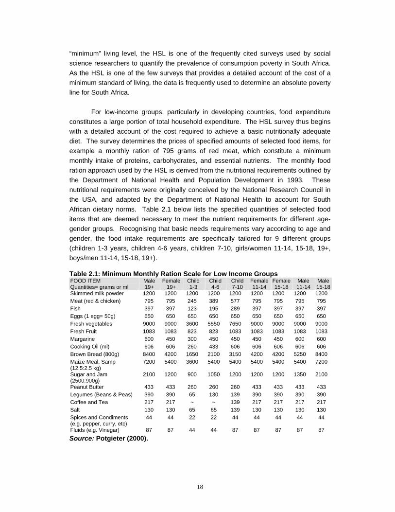
For low-income groups, particularly in developing countries, food expenditure constitutes a large portion of total household expenditure. The HSL survey thus begins with a detailed account of the cost required to achieve a basic nutritionally adequate diet. The survey determines the prices of specified amounts of selected food items, for example a monthly ration of 795 grams of red meat, which constitute a minimum monthly intake of proteins, carbohydrates, and essential nutrients. The monthly food ration approach used by the HSL is derived from the nutritional requirements outlined by the Department of National Health and Population Development in 1993. These nutritional requirements were originally conceived by the National Research Council in the USA, and adapted by the Department of National Health to account for South African dietary norms. Table 2.1 below lists the specified quantities of selected food items that are deemed necessary to meet the nutrient requirements for different age-gender groups. Recognising that basic needs requirements vary according to age and gender, the food intake requirements are specifically tailored for 9 different groups (children 1-3 years, children 4-6 years, children 7-10, girls/women 11-14, 15-18, 19+, boys/men 11-14, 15-18, 19+). Table 2.1: Minimum Monthly Ration Scale for Low Income Groups FOOD ITEM Quantities= grams or ml
Male 19+
Female19+
Child 1-3
Child 4-6
Child 7-10
Female11-14
Female 15-18
Male 11-14
Male15-18
Skimmed milk powder 1200 1200 1200 1200 1200 1200 1200 1200 1200 Meat (red & chicken) 795 795 245 389 577 795 795 795 795 Fish 397 397 123 195 289 397 397 397 397 Eggs (1 egg= 50g) 650 650 650 650 650 650 650 650 650 Fresh vegetables 9000 9000 3600 5550 7650 9000 9000 9000 9000 Fresh Fruit 1083 1083 823 823 1083 1083 1083 1083 1083 Margarine 600 450 300 450 450 450 450 600 600 Cooking Oil (ml) 606 606 260 433 606 606 606 606 606 Brown Bread (800g) 8400 4200 1650 2100 3150 4200 4200 5250 8400 Maize Meal, Samp (12.5:2.5 kg)
7200 5400 3600 5400 5400 5400 5400 5400 7200
Sugar and Jam (2500:900g)
2100 1200 900 1050 1200 1200 1200 1350 2100
Peanut Butter 433 433 260 260 260 433 433 433 433 Legumes (Beans & Peas) 390 390 65 130 139 390 390 390 390 Coffee and Tea 217 217 ~ ~ 139 217 217 217 217 Salt 130 130 65 65 139 130 130 130 130 Spices and Condiments (e.g. pepper, curry, etc)
44 44 22 22 44 44 44 44 44
Fluids (e.g. Vinegar) 87 87 44 44 87 87 87 87 87 Source: Potgieter (2000).
19
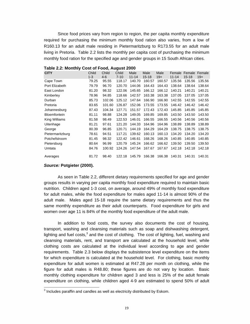
Since food prices vary from region to region, the per capita monthly expenditure required for purchasing the minimum monthly food ration also varies, from a low of R160.13 for an adult male residing in Pietermaritzburg to R173.55 for an adult male living in Pretoria. Table 2.2 lists the monthly per capita cost of purchasing the minimum monthly food ration for the specified age and gender groups in 15 South African cities.
Table 2.2: Monthly Cost of Food, August 2000
CITY Child 1-3
Child 4-6
Child 7-10
Male 11-14
Male 15-18
Male 19+
Female 11-14
Female 15-18
Female19+
Cape Town 79.25 95.55 118.17 140.70 160.57 160.57 135.56 135.56 135.56Port Elizabeth 79.79 96.70 120.70 144.06 164.43 164.43 138.64 138.64 138.64East London 81.20 98.32 122.06 145.65 166.12 166.12 140.21 140.21 140.21Kimberley 78.96 94.85 118.66 142.57 163.38 163.38 137.05 137.05 137.05Durban 85.73 102.06 125.12 147.64 166.90 166.90 142.55 142.55 142.55Pretoria 83.65 101.60 126.87 152.06 173.55 173.55 146.42 146.42 146.42Johannesburg 87.43 104.34 127.71 151.57 172.43 172.43 145.85 145.85 145.85Bloemfontein 81.11 98.88 124.28 149.05 169.85 169.85 143.50 143.50 143.50King Williams 81.58 98.49 122.53 146.01 166.55 166.55 140.56 140.56 140.56Uitenhage 81.21 97.61 121.20 144.33 164.96 164.96 138.89 138.89 138.89George 80.39 96.85 120.71 144.19 164.29 164.29 138.75 138.75 138.75Pietermaritzburg 78.61 94.51 117.21 139.62 160.13 160.13 134.20 134.20 134.20Potchefstroom 81.45 98.32 122.42 146.61 168.26 168.26 140.85 140.85 140.85Pietersburg 80.64 96.99 120.79 145.24 166.62 166.62 139.50 139.50 139.50Umtata 84.76 100.92 124.26 147.54 167.67 167.67 142.18 142.18 142.18 Averages
81.72 98.40 122.18 145.79 166.38 166.38 140.31 140.31 140.31
Source: Potgieter (2000).
As seen in Table 2.2, different dietary requirements specified for age and gender groups results in varying per capita monthly food expenditure required to maintain basic nutrition. Children aged 1-3 cost, on average, around 49% of monthly food expenditure for adult males, while the food expenditure for males aged 11-14 is almost 90% of the adult male. Males aged 15-18 require the same dietary requirements and thus the same monthly expenditure as their adult counterparts. Food expenditure for girls and women over age 11 is 84% of the monthly food expenditure of the adult male.
In addition to food costs, the survey also documents the cost of housing,
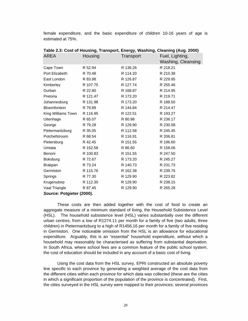
transport, washing and cleansing materials such as soap and dishwashing detergent, lighting and fuel costs,3 and the cost of clothing. The cost of lighting, fuel, washing and cleansing materials, rent, and transport are calculated at the household level, while clothing costs are calculated at the individual level according to age and gender requirements. Table 2.3 below displays the subsistence level expenditure on the items for which expenditure is calculated at the household level. For clothing, basic monthly expenditure for adult women is estimated at R47.28 per month on clothing, while the figure for adult males is R48.80; these figures are do not vary by location. Basic monthly clothing expenditure for children aged 3 and less is 25% of the adult female expenditure on clothing, while children aged 4-9 are estimated to spend 50% of adult 3 Includes paraffin and candles as well as electricity distributed by Eskom.
20
female expenditure, and the basic expenditure of children 10-16 years of age is estimated at 75%. Table 2.3: Cost of Housing, Transport, Energy, Washing, Cleaning (Aug. 2000) AREA
Housing Transport Fuel, Lighting, Washing, Cleansing
Cape Town R 52.94 R 136.26 R 218.21 Port Elizabeth R 70.48 R 114.20 R 210.38 East London R 83.98 R 126.87 R 229.95 Kimberley R 107.75 R 127.74 R 255.46 Durban R 22.80 R 168.87 R 214.95 Pretoria R 121.47 R 173.20 R 219.71 Johannesburg R 131.98 R 173.20 R 188.50 Bloemfontein R 79.89 R 144.84 R 214.47 King Williams Town R 116.95 R 122.51 R 193.27 Uitenhage R 65.07 R 80.98 R 236.17 George R 79.28 R 129.90 R 230.58 Pietermaritzburg R 35.05 R 112.58 R 245.45 Potchefstroom R 68.54 R 116.91 R 206.81 Pietersburg R 42.45 R 151.55 R 196.60 Umtata R 152.58 R 86.60 R 158.06 Benoni R 100.83 R 151.55 R 247.50 Boksburg R 72.67 R 173.20 R 245.27 Brakpan R 73.24 R 140.73 R 231.73 Germiston R 115.76 R 162.38 R 239.75 Springs R 77.30 R 129.90 R 223.82 Krugersdorp R 112.30 R 129.90 R 238.15 Vaal Triangle R 87.45 R 129.90 R 265.28 Source: Potgieter (2000).
These costs are then added together with the cost of food to create an aggregate measure of a minimum standard of living, the Household Subsistence Level (HSL). The household subsistence level (HSL) varies substantially over the different urban centres, from a low of R1274.11 per month for a family of five (two adults, three children) in Pietermaritzburg to a high of R1456.16 per month for a family of five residing in Germiston. One noticeable omission from the HSL is an allowance for educational expenditure. Arguably, this is an “essential” household expenditure, without which a household may reasonably be characterised as suffering from substantial deprivation. In South Africa, where school fees are a common feature of the public school system, the cost of education should be included in any account of a basic cost of living.
Using the cost data from the HSL survey, EPRI constructed an absolute poverty
line specific to each province by generating a weighted average of the cost data from the different cities within each province for which data was collected (these are the cities in which a significant proportion of the population of the province is concentrated). First, the cities surveyed in the HSL survey were mapped to their provinces; several provinces
21
had cost data collected from more than one city (Western Cape, Eastern Cape, KwaZulu Natal, and Gauteng province), several provinces had cost data collected from one city only (Northern Cape, Free State, North West, and Limpopo province), and one province did not have cost data from any city (Mpumalanga). The cost data for Limpopo was used to proxy for the missing data in Mpumalanga, based on the geographic proximity of the two provinces and thus the assumption of similar costs of living. Then, the populations of the cities in the surveys were determined and verified. Subsequently, the cost data for those provinces with more than one city surveyed was then weighted according to the populations of the cities in order to arrive at one set of cost data for each province. The weighted cost data derived from the HSL survey was then merged with the Income and Expenditure 2000 database in order to calculate a minimum subsistence level. Thus, each household in the database has a uniquely determined poverty line, depending on the province of residence and the specific demographic makeup of the household.
The strength of the HSL cost data is that it allows researchers to account for
differences in purchasing power across provinces. Furthermore, the HSL poverty line accounts for varying nutritional needs of different age-gender groups. Empirical evidence does suggest that the caloric requirements of children are less than that of adult males, and thus the per capita expenditure requirements are lower as well.4
Although there are still some institutions calculating minimum subsistence levels,
recently there has been a shift away from the use of absolute poverty lines in favour of using relative poverty lines, due to concern over a number of methodological shortcomings associated with absolute poverty lines.
The most often cited problem is that absolute poverty lines require an extremely subjective assessment of what constitutes a minimally acceptable standard of living. For example, is the satisfaction of basic nutritional needs sufficient, or should an absolute poverty measure also include monetary allowances for important social expenditures such as education and health services? What about more abstract basic needs, such as the rights of self-determination, which are vitally important but difficult or impossible to quantify?
Another important methodological issue associated with absolute poverty lines is the problem of over generalisation. The poverty line applies to all units in the poverty domain, which means that differences related to particular sub-groups cannot be accounted for. An income that is sufficient in an urban setting may not be sufficient in a rural area, due to pronounced differences in purchasing power or varying basic needs. Furthermore, different social groups may have different tastes or eating habits, which may result in variations in their respective basic costs of living. This problem is particularly relevant in South Africa, where rural and urban and racial disparities are acute and historically entrenched. However, creating different poverty lines for different subgroups is probably not a feasible solution, as it involves additional levels of subjectivity and renders comparisons across subgroups less meaningful.
4 Woolard and Leibbrandt (1999).
22
Finally, the detailed cost data needed to construct an absolute poverty line may be difficult to collect or obtain in a developing country. Obtaining a national average of the cost of a basket of necessities is undoubtedly a difficult and time-consuming process, and in South Africa, only a handful of organisations have produced such data. For these aforementioned reasons, many researchers undertaking poverty analysis opt to use relative poverty lines, which define poverty in relation to other members of the poverty domain.
A relative poverty line can be defined as that income level that cuts off the specified poorest percentage of the population. The poor are those persons who suffer deprivation relative to others in the poverty domain.5 For example, the World Bank generally defines the ‘poor’ as the bottom forty percent of households, and defines the “destitute” as the bottom twenty- percent of the income distribution. The relative poverty line is generally more widely used than the absolute poverty line, as it is much easier to construct. Furthermore, calculations with the relative poverty line are less likely to be controversial, as they avoid the subjectivity associated with determining what income or expenditure threshold constitutes a minimal acceptable standard of living.
For South Africa, the relative poverty line that delineates the bottom 40% of households is R459 per person per month in September 2000, when economies of scale and adult equivalency scales are applied. Without economies of scale and adult equivalency scales, the comparable figure is R345 per person per month. The comparable figures for income poverty are R423 (with scales) and R319 per person per month (without scales). METHODOLOGICAL ISSUES: INCOME VERSUS EXPENDITURE POVERTY
Another methodological issue to address when constructing a poverty line is whether income or expenditure more accurately captures the extent of consumption poverty experienced by households. As Ravallion (1992) and Deaton (1997) suggest, expenditure may be the preferred measure in developing countries. First, expenditure is a much more direct measure of consumption than income, and thus may more accurately reflect the degree of commodity deprivation and provide a more reliable indicator of household welfare. Whether a household or individual consumes enough of basic needs (food) is more directly related to their welfare than how much income they earn. Second, reporting of income is notoriously flawed, for a number of different reasons. Accounting for all sources of income, including such diverse sources as different types of private transfers such as loans, remittances, and inheritances, wages, returns on capital, gifts-in-kind and in cash, and employee benefits, is difficult in any setting, and is perhaps made even more difficult in developing countries where the resources for data collection are more limited. Furthermore, there is some evidence that respondents in surveys systematically underreport income, though the exact motives underlying this dynamic is unclear. Finally, there is some evidence that expenditure is more stable and perhaps more reliable than income, particularly amongst the poor. During times of economic hardship, people are likely to undertake consumption-smoothing activities, such as borrowing or using savings (Ravallion, 1992). Thus, expenditure may provide a more accurate measure of well being than income. Indeed, two important papers written on the topic of measuring poverty in South Africa 5 Woolard and Leibbrandt (1999).
23
(NIEP, 2001; Woolard and Leibbrandt, 1999) both select the expenditure measure for the aforementioned reasons.
However, using income as an indicator of welfare may also be useful in specific situations. This study seeks to measure the impact of specific poverty interventions on the face of poverty in South Africa. In South Africa, the means test for qualifying for social grants is determined using income rather than expenditure. Thus, for the purposes of this study it may be more intuitively obvious to use income thresholds to determine who is poor, as this is the method by which social assistance grants are allocated. Furthermore, social grants directly raise income by 100% of the value of the grant, while only raising expenditure by a proportion. EPRI has thus chosen to use both measures, which is also important for the purpose of confirming the robustness of the results. METHODOLOGICAL ISSUES: EQUIVALENCE SCALES
Researchers working with poverty lines have grappled with the issue of accounting for possible age and gender-based differences in consumption behaviour. If it is indeed the case that children and women cost less than adult males, should children and women be weighted as less than one adult male equivalent for the purposes of deriving a poverty line? If so, how should the exact magnitude of the weights be determined? International research suggests that children may consume less food than adult males, but does this relationship necessarily hold with respect to non-food expenditure? Another dynamic that researchers have attempted to quantify is the effect of economies of scale. Household size may affect the consumption needs of households in a non-linear relationship; larger households may need less income on a per capita basis than smaller households, due to the effect of economies of scale. Many expenses may not depend on the size of the family (for example, rent, or in some cases fuel), and thus larger households benefit as these shared costs are spread over a greater number of people than in a smaller household.
In some of the literature concerned with deriving a poverty line for South Africa, the convention has been to weight children under eighteen as half of an adult equivalent, while applying an exponential scale of 0.9 to account for economies of scale, as in the work of May et al (1995). However, these numbers are not grounded in any empirical studies of household economies in South Africa. Thus, applying equivalence scales may or may not be appropriate for poverty analysis in South Africa, in the absence of more specific analysis of South Africa’s consumption patterns and the intra-household allocation of resources.
As indicated earlier, the purpose of the discussion here is not to determine an appropriate poverty line for South Africa, but instead to highlight some of the methodological issues associated with selecting a poverty line. Indeed, in the interests of systematic rigour and reliability, EPRI has chosen to use several different poverty lines for the impact analysis in this study, both absolute and relative. Both relative and absolute poverty lines require the definition of a specific income or expenditure threshold, which involves an element of arbitrariness. Measured poverty rates may be very sensitive to small changes in the poverty datum, depending on the shape of the income distribution in the poverty domain. Thus, using a number of different poverty

24
lines is important to confirm the robustness of the results when measuring the impact of different poverty interventions METHODOLOGICAL ISSUES: THE POVERTY HEADCOUNT AND OTHER POVERTY MEASURES
The poverty headcount, which is simply the number of individuals or households falling below a given income/expenditure threshold, provides a conceptual tool in quantifying the extent of deprivation within a country. However, using the poverty line to determine the poverty headcount has a number of shortcomings, particularly when measuring changes in poverty over time. EPRI has chosen to supplement the poverty headcount with a number of other poverty measures that together paint a fuller picture of the face of poverty in South Africa.
The poverty datum line sets a particular income or expenditure threshold, which delineates whether or not a household is considered poor. However, those households and individuals who arguably need the most assistance (the poorest) may not move above the poverty line after a given poverty intervention. A household may gain a Child Support Grant under a new policy, but this R100 extra per month may not cause the new household income to exceed the poverty threshold. Yet this increase in income may indeed result in a qualitative change in the household’s welfare, an improvement that is not captured by the poverty headcount measure. Thus, a poverty intervention that is well targeted (i.e. impacts the poorest) may actually result in a much smaller change in the poverty rate than a less well targeted intervention (i.e. impacts the wealthiest of the poor whose incomes are clustered near the poverty line). Undoubtedly, the effect of poverty interventions on the poorest is likely to be of interest to policymakers; for this reason, EPRI has supplemented the poverty headcount measure with a number of different poverty gap measures.
The poverty gap measures the difference between a household’s income (or expenditure) and the poverty line. By using a poverty gap measure, the impact of a poverty intervention is captured regardless of whether a household moves above the poverty line, as the household’s poverty gap will be reduced by the exact amount of the grant (at least up to the point where the household escapes poverty). This study uses three different kinds of poverty gap measures. First, the average poverty gap measures the difference between the households’ total incomes and the poverty line, then takes the average of the differences over a given domain (for example, a province). Second, the percentage poverty gap takes each household’s poverty gap and divides it by the poverty line, and calculates the average across all households. Finally, the total rand poverty gap aggregates the poverty gap of each household over a given domain. This figure is particularly useful to policymakers, as it allows them to estimate of the aggregate cost of a particular policy intervention, assuming perfect targeting. Using both poverty gap measures and the poverty headcount measure provides a more nuance understanding of the poverty-reducing impact of policy interventions.
25
2.3) THE EPRI MICRO-SIMULATION MODEL The EPRI micro-simulation model was calibrated using three data sources:
Statistics South Africa’s September 2000 Income and Expenditure Survey, the September 2000 Labour Force Survey and administrative data from the Department of Social Development. The Income and Expenditure Survey (I&E) provides measures of social assistance take-up as well as detailed profiles of the income and expenditure patterns of the surveyed households. The Labour Force Survey provides the additional demographic information required to determine eligibility for the social assistance grants; furthermore, it provides detailed information on labour market activity and various measures of well-being such as access to public services. The Department of Social Development’s administrative data provides actual take-up figures by grant by province, as well as additional information. THE MICRO-SIMULATION MODEL: POVERTY LINES
In consultation with the Department of Social Development, EPRI selected several poverty lines for the analysis. The absolute poverty line is based on the Household Subsistence Level Survey. The destitution poverty line is based on household expenditure; calculating relative destitution based on the lowest income 20% of households in the income distribution. This lower bound poverty line (or “destitution” poverty line) supports the analysis of proposed policy changes on the poorest segment of society. The destitution line is scaled—that is, it is adjusted for economies of scale and adult equivalency factors. The rand amount that resulted in 20% of households in the population being designated as “poor” is R180 per person per month. In addition, a relative expenditure poverty line was calculated based on the threshold separating the lowest expenditure 40% of households. Scaled and unscaled income and expenditure poverty lines were calculated based on the terms of reference of the Taylor Committee of Inquiry, set at R394 per person per month.6 The income and expenditure scaled poverty lines apply the economies of scale and adult equivalency scales.7 These poverty lines, while not exhaustive, cover a range of the methodological issues discussed in the previous section. Furthermore, the use of different poverty lines allows the measurement of the sensitivity of the results.
The main purpose of the EPRI micro-simulation model is to assess the impact of the current system of social grants on poverty alleviation, as well as to gauge the potential impact of proposed policy reforms and poverty interventions. The scenarios modelled using the micro-simulation tool were developed in consultation with working group meetings at the Department of Social Development, and focus on three social assistance grants: the State Old Age Pension (SOAP), the Child Support Grant (CSG), and the Disability Grant (DG). This section of the report will review the methodology underlying the micro-simulation modelling generally and for each specific grant, as well as discuss some of the difficulties encountered during the task of calibrating the model with household survey data.
6 This figure is slightly different from the stated figure R401 per capita, as it has been deflated to September 2000 terms using Statistics South Africa’s inflation series data. 7 The adult equivalency scale is set at 0.5 and the economies of scale figure is set at 0.9.
26
THE MICRO-SIMULATION MODEL: AN OVERVIEW OF THE MODELLING SCENARIOS
In this study’s analysis, the baseline scenario is taken to be the level of social assistance take-up in September 2000, as measured using the Income and Expenditure Survey. In September 2000, an estimated 2.7 million individuals were receiving some sort of social assistance grant, with approximately 460,000 CSG recipients, 440,000 DG recipients, and 1.8 million SOAP recipients. In all of the modelling scenarios, these take-up rates are used as the baseline against which the impact of all other policy reforms/modelling scenarios are evaluated and compared.
Using the poverty lines detailed above, EPRI researchers measured the poverty-reducing impact of a variety of possible scenarios with the CGS, DG, and the SOAP. The first scenario evaluated the extent to which the social security system reduced the extent of measured poverty in September 2000. The Income and Expenditure Survey contains detailed information on the income of households, including the monetary amount of each social assistance grant received. In September 2000, this amount was R100 per recipient per month for the CSG and R540 per recipient per month for both the DG and the SOAP. By removing the monetary amount of all social grants from the total household income and subsequently measuring the resulting poverty in the absence of all social assistance, the study quantifies the impact of the social security system in September 2000.
In addition, the EPRI micro-simulation model was used to simulate the effect of increased take-up of each grant, such as a 10% increase in take-up of the SOAP, a 50% increase in the take-up of the DG, and increases to full take-up for all the grants. The simulation of full take-up of each grant under the existing eligibility criteria (making strong assumptions) provides a sense of the upper bound of the poverty impact of the social security programme. In addition, the effects of policy reforms (the extension of the CSG to children up to age 14 in several stages, as well as the hypothetical extensions to age 16 and age 18) were modelled and the poverty impact measured. Each modelling scenario was analysed using the poverty lines discussed above. The poverty headcount, as well as the average, rand, and percentage poverty gap, were calculated for each scenario, in order to provide a detailed picture of the poverty impact of each scenario. The simulations evaluate the impact of extensions in scope and increases in take-up of the grants, not in changes in grant amount, with the exception of the CSG, for which both real 2000 and real 2003 grant amounts were evaluated. THE STATE OLD-AGE PENSION
According to the guidelines obtained from the Department of Social Development, eligibility for the SOAP is determined according to both an age and a means test. During the sample period male recipients had to be over 65 years of age, while female recipients had to be over 60 years of age. In addition, if the individual was single his/her income must have fallen below R1226 per month, and if the individual was married his/her income must have fall below R2226 per month. The median amount of

27
the grant in September 2000 was R540 per recipient per month. According to this particular eligibility criterion, there were approximately 2.2 million age and income eligible SOAP recipients in South Africa in September of 2000. Of these eligible recipients, nearly 1.8 million were already receiving the grant in September 2000, while approximately 400,000 were eligible but not receiving the grant. Unlike with the CSG and the DG, the take-up rate for the SOAP in September 2000 was already quite high, over eighty percent of the total number of eligible recipients. Table 2.4 below breaks down the number of grants and the resulting take-up rate by province: Table 2.4: Take-up of State Old-Age Pension by Province, September 2000
National/ Province
# Grant Recipients, take-up rate
Number (#) of eligible recipients
Take-up rate
# of eligible recipients not
receiving SOAP
National 1767591 2185321 80.9% 417730 Western Cape 115210 144048 80.0% 28838 Eastern Cape 359973 440935 81.6% 80962 Northern Cape 30040 37530 80.0% 7490
Free State 93003 115723 80.4% 22720 KwaZulu Natal 358184 445656 80.4% 87472
Northwest 139114 167269 83.2% 28155 Gauteng 304931 414663 73.5% 109732
Mpumalanga 97852 110697 88.4% 12845 Limpopo 269284 308800 87.2% 39516
Source: Income & Expenditure 2000 THE CHILD SUPPORT GRANT
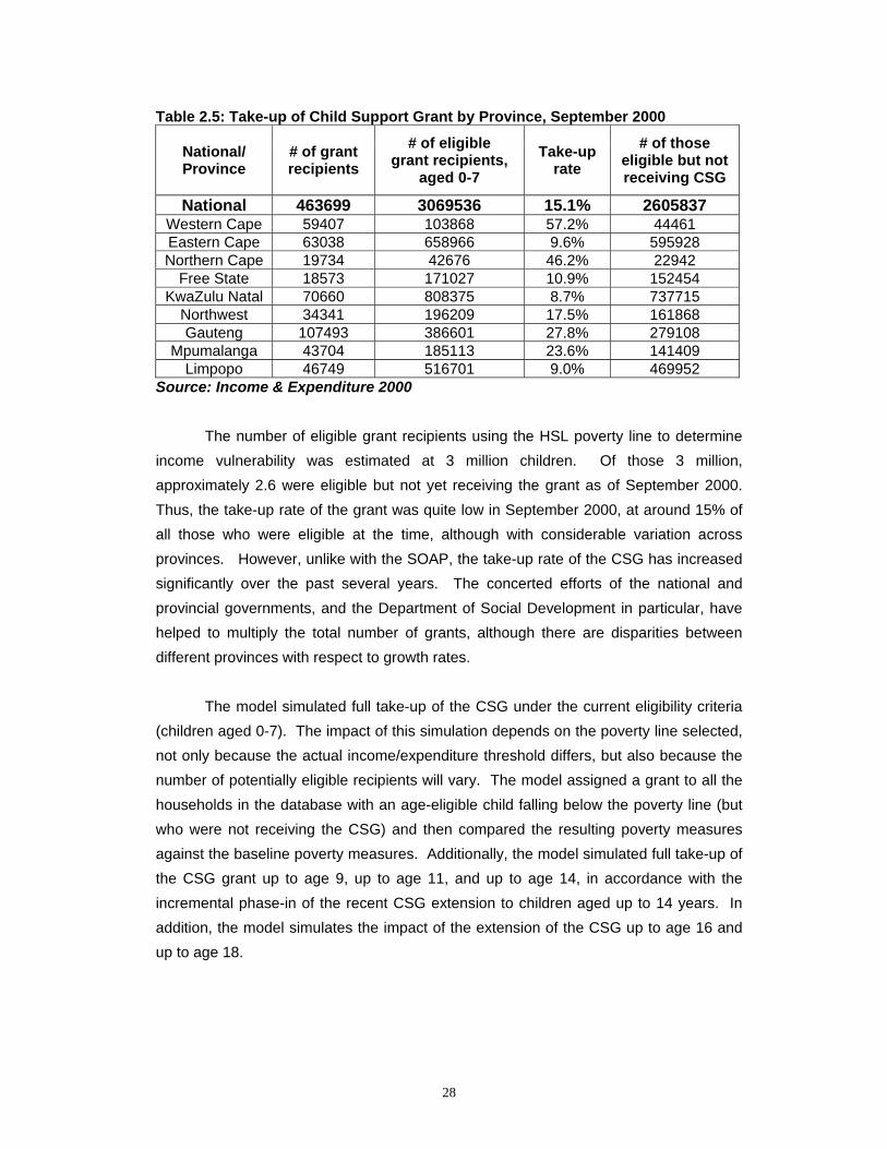
Modelling Child Support Grant scenarios with the model raised methodological and data quality issues. The Income and Expenditure Survey does not collect data on the different child-related grants separately, but rather aggregates them together under one category. As a result, the analysis of the baseline September 2000 take-up rates cannot differentiate between recipients of the CSG, the Foster Care Grant, and the Care Dependency Grant in September 2000. In addition, neither the Income and Expenditure Survey nor the Labour Force Survey contains information on the identity of the primary caregiver of the child. EPRI’s model bases take-up analysis on household income or expenditure vulnerability; assigning grants to those households (with an age-eligible child) whose total income falls below that of the particular poverty line used for the analysis.
28
Table 2.5: Take-up of Child Support Grant by Province, September 2000
National/ Province
# of grant recipients
# of eligible grant recipients,
aged 0-7 Take-up
rate # of those
eligible but not receiving CSG
National 463699 3069536 15.1% 2605837 Western Cape 59407 103868 57.2% 44461 Eastern Cape 63038 658966 9.6% 595928 Northern Cape 19734 42676 46.2% 22942
Free State 18573 171027 10.9% 152454 KwaZulu Natal 70660 808375 8.7% 737715
Northwest 34341 196209 17.5% 161868 Gauteng 107493 386601 27.8% 279108
Mpumalanga 43704 185113 23.6% 141409 Limpopo 46749 516701 9.0% 469952
Source: Income & Expenditure 2000
The number of eligible grant recipients using the HSL poverty line to determine income vulnerability was estimated at 3 million children. Of those 3 million, approximately 2.6 were eligible but not yet receiving the grant as of September 2000. Thus, the take-up rate of the grant was quite low in September 2000, at around 15% of all those who were eligible at the time, although with considerable variation across provinces. However, unlike with the SOAP, the take-up rate of the CSG has increased significantly over the past several years. The concerted efforts of the national and provincial governments, and the Department of Social Development in particular, have helped to multiply the total number of grants, although there are disparities between different provinces with respect to growth rates.
The model simulated full take-up of the CSG under the current eligibility criteria (children aged 0-7). The impact of this simulation depends on the poverty line selected, not only because the actual income/expenditure threshold differs, but also because the number of potentially eligible recipients will vary. The model assigned a grant to all the households in the database with an age-eligible child falling below the poverty line (but who were not receiving the CSG) and then compared the resulting poverty measures against the baseline poverty measures. Additionally, the model simulated full take-up of the CSG grant up to age 9, up to age 11, and up to age 14, in accordance with the incremental phase-in of the recent CSG extension to children aged up to 14 years. In addition, the model simulates the impact of the extension of the CSG up to age 16 and up to age 18.
29
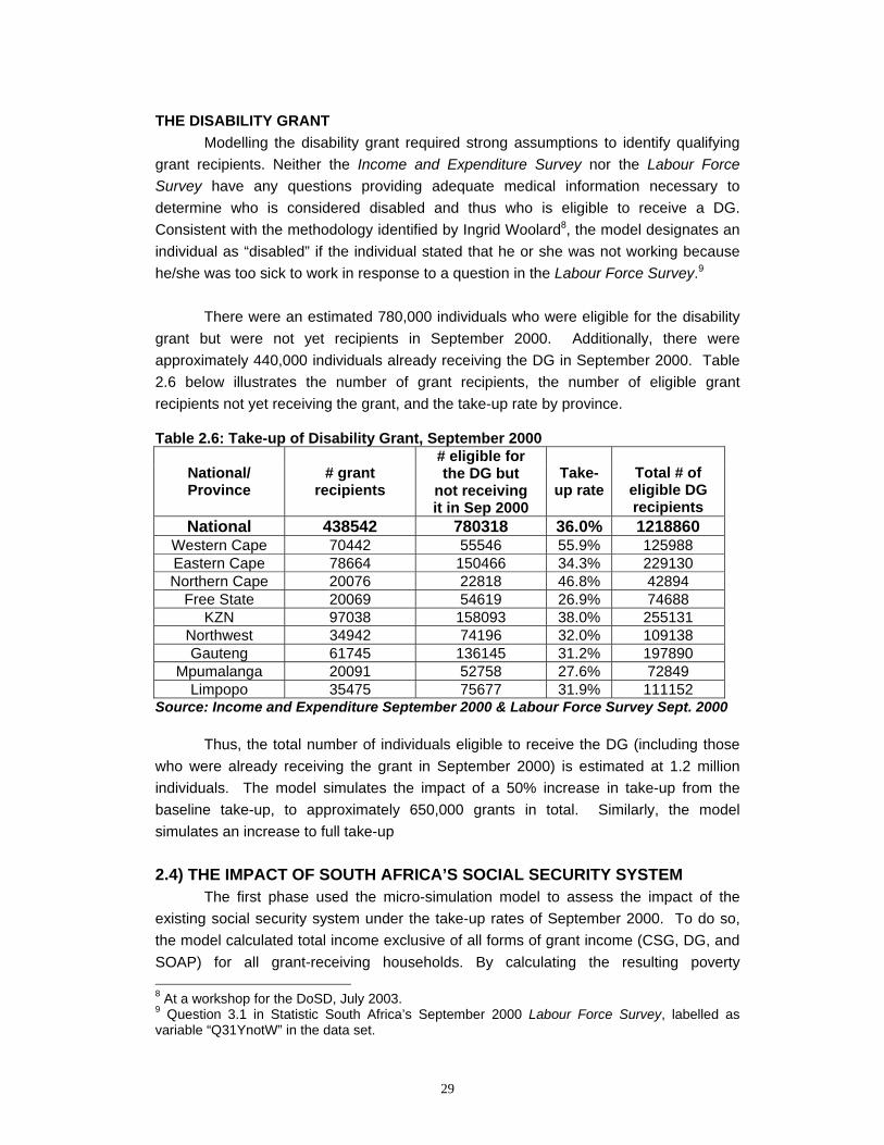
THE DISABILITY GRANT Modelling the disability grant required strong assumptions to identify qualifying
grant recipients. Neither the Income and Expenditure Survey nor the Labour Force Survey have any questions providing adequate medical information necessary to determine who is considered disabled and thus who is eligible to receive a DG. Consistent with the methodology identified by Ingrid Woolard8, the model designates an individual as “disabled” if the individual stated that he or she was not working because he/she was too sick to work in response to a question in the Labour Force Survey.9
There were an estimated 780,000 individuals who were eligible for the disability grant but were not yet recipients in September 2000. Additionally, there were approximately 440,000 individuals already receiving the DG in September 2000. Table 2.6 below illustrates the number of grant recipients, the number of eligible grant recipients not yet receiving the grant, and the take-up rate by province. Table 2.6: Take-up of Disability Grant, September 2000
National/ Province
# grant recipients
# eligible for the DG but
not receiving it in Sep 2000
Take-up rate
Total # of eligible DG recipients
National 438542 780318 36.0% 1218860 Western Cape 70442 55546 55.9% 125988 Eastern Cape 78664 150466 34.3% 229130 Northern Cape 20076 22818 46.8% 42894
Free State 20069 54619 26.9% 74688 KZN 97038 158093 38.0% 255131
Northwest 34942 74196 32.0% 109138 Gauteng 61745 136145 31.2% 197890
Mpumalanga 20091 52758 27.6% 72849 Limpopo 35475 75677 31.9% 111152
Source: Income and Expenditure September 2000 & Labour Force Survey Sept. 2000
Thus, the total number of individuals eligible to receive the DG (including those who were already receiving the grant in September 2000) is estimated at 1.2 million individuals. The model simulates the impact of a 50% increase in take-up from the baseline take-up, to approximately 650,000 grants in total. Similarly, the model simulates an increase to full take-up 2.4) THE IMPACT OF SOUTH AFRICA’S SOCIAL SECURITY SYSTEM
The first phase used the micro-simulation model to assess the impact of the existing social security system under the take-up rates of September 2000. To do so, the model calculated total income exclusive of all forms of grant income (CSG, DG, and SOAP) for all grant-receiving households. By calculating the resulting poverty 8 At a workshop for the DoSD, July 2003. 9 Question 3.1 in Statistic South Africa’s September 2000 Labour Force Survey, labelled as variable “Q31YnotW” in the data set.
30
headcount and the poverty gap measures in the absence of social assistance, the model effectively quantifies the impact of the current system of grants, under September 2000 take-up rates. This analysis used the poverty lines established in conjunction with the DoSD and described above.
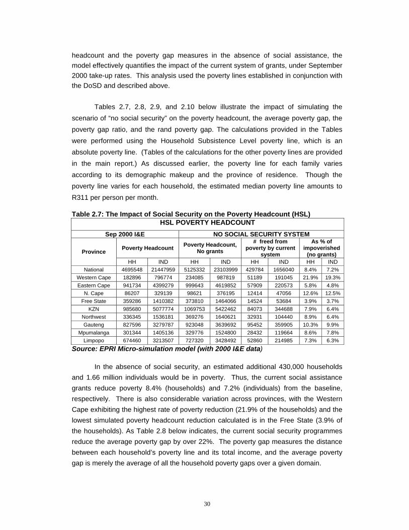
Tables 2.7, 2.8, 2.9, and 2.10 below illustrate the impact of simulating the scenario of “no social security” on the poverty headcount, the average poverty gap, the poverty gap ratio, and the rand poverty gap. The calculations provided in the Tables were performed using the Household Subsistence Level poverty line, which is an absolute poverty line. (Tables of the calculations for the other poverty lines are provided in the main report.) As discussed earlier, the poverty line for each family varies according to its demographic makeup and the province of residence. Though the poverty line varies for each household, the estimated median poverty line amounts to R311 per person per month. Table 2.7: The Impact of Social Security on the Poverty Headcount (HSL)
HSL POVERTY HEADCOUNT Sep 2000 I&E NO SOCIAL SECURITY SYSTEM
Poverty Headcount Poverty Headcount, No grants
# freed from poverty by current
system
As % of impoverished
(no grants) Province
HH IND HH IND HH IND HH IND National 4695548 21447959 5125332 23103999 429784 1656040 8.4% 7.2%
Western Cape 182896 796774 234085 987819 51189 191045 21.9% 19.3% Eastern Cape 941734 4399279 999643 4619852 57909 220573 5.8% 4.8%
N. Cape 86207 329139 98621 376195 12414 47056 12.6% 12.5% Free State 359286 1410382 373810 1464066 14524 53684 3.9% 3.7%
KZN 985680 5077774 1069753 5422462 84073 344688 7.9% 6.4% Northwest 336345 1536181 369276 1640621 32931 104440 8.9% 6.4% Gauteng 827596 3279787 923048 3639692 95452 359905 10.3% 9.9%
Mpumalanga 301344 1405136 329776 1524800 28432 119664 8.6% 7.8% Limpopo 674460 3213507 727320 3428492 52860 214985 7.3% 6.3%
Source: EPRI Micro-simulation model (with 2000 I&E data)
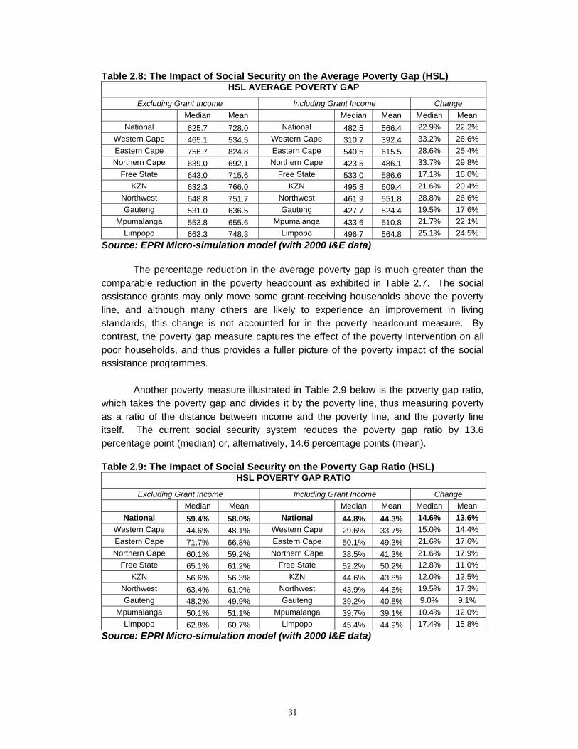
In the absence of social security, an estimated additional 430,000 households and 1.66 million individuals would be in poverty. Thus, the current social assistance grants reduce poverty 8.4% (households) and 7.2% (individuals) from the baseline, respectively. There is also considerable variation across provinces, with the Western Cape exhibiting the highest rate of poverty reduction (21.9% of the households) and the lowest simulated poverty headcount reduction calculated is in the Free State (3.9% of the households). As Table 2.8 below indicates, the current social security programmes reduce the average poverty gap by over 22%. The poverty gap measures the distance between each household’s poverty line and its total income, and the average poverty gap is merely the average of all the household poverty gaps over a given domain.
31
Table 2.8: The Impact of Social Security on the Average Poverty Gap (HSL) HSL AVERAGE POVERTY GAP
Excluding Grant Income Including Grant Income Change Median Mean Median Mean Median Mean
National 625.7 728.0 National 482.5 566.4 22.9% 22.2% Western Cape 465.1 534.5 Western Cape 310.7 392.4 33.2% 26.6% Eastern Cape 756.7 824.8 Eastern Cape 540.5 615.5 28.6% 25.4% Northern Cape 639.0 692.1 Northern Cape 423.5 486.1 33.7% 29.8%
Free State 643.0 715.6 Free State 533.0 586.6 17.1% 18.0% KZN 632.3 766.0 KZN 495.8 609.4 21.6% 20.4%
Northwest 648.8 751.7 Northwest 461.9 551.8 28.8% 26.6% Gauteng 531.0 636.5 Gauteng 427.7 524.4 19.5% 17.6%
Mpumalanga 553.8 655.6 Mpumalanga 433.6 510.8 21.7% 22.1% Limpopo 663.3 748.3 Limpopo 496.7 564.8 25.1% 24.5%
Source: EPRI Micro-simulation model (with 2000 I&E data)
The percentage reduction in the average poverty gap is much greater than the comparable reduction in the poverty headcount as exhibited in Table 2.7. The social assistance grants may only move some grant-receiving households above the poverty line, and although many others are likely to experience an improvement in living standards, this change is not accounted for in the poverty headcount measure. By contrast, the poverty gap measure captures the effect of the poverty intervention on all poor households, and thus provides a fuller picture of the poverty impact of the social assistance programmes.
Another poverty measure illustrated in Table 2.9 below is the poverty gap ratio, which takes the poverty gap and divides it by the poverty line, thus measuring poverty as a ratio of the distance between income and the poverty line, and the poverty line itself. The current social security system reduces the poverty gap ratio by 13.6 percentage point (median) or, alternatively, 14.6 percentage points (mean). Table 2.9: The Impact of Social Security on the Poverty Gap Ratio (HSL)
HSL POVERTY GAP RATIO
Excluding Grant Income Including Grant Income Change Median Mean Median Mean Median Mean
National 59.4% 58.0% National 44.8% 44.3% 14.6% 13.6% Western Cape 44.6% 48.1% Western Cape 29.6% 33.7% 15.0% 14.4% Eastern Cape 71.7% 66.8% Eastern Cape 50.1% 49.3% 21.6% 17.6% Northern Cape 60.1% 59.2% Northern Cape 38.5% 41.3% 21.6% 17.9%
Free State 65.1% 61.2% Free State 52.2% 50.2% 12.8% 11.0% KZN 56.6% 56.3% KZN 44.6% 43.8% 12.0% 12.5%
Northwest 63.4% 61.9% Northwest 43.9% 44.6% 19.5% 17.3% Gauteng 48.2% 49.9% Gauteng 39.2% 40.8% 9.0% 9.1%
Mpumalanga 50.1% 51.1% Mpumalanga 39.7% 39.1% 10.4% 12.0% Limpopo 62.8% 60.7% Limpopo 45.4% 44.9% 17.4% 15.8%
Source: EPRI Micro-simulation model (with 2000 I&E data)
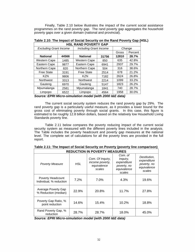
32
Finally, Table 2.10 below illustrates the impact of the current social assistance programmes on the rand poverty gap. The rand poverty gap aggregates the household poverty gaps over a given domain (national and provincial). Table 2.10: The Impact of Social Security on the Rand Poverty Gap (HSL)
HSL RAND POVERTY GAP Excluding Grant Income Including Grant Income Change
Gross Percent National 44566 National 31756 12810 28.7%
Western Cape 1485 Western Cape 850 635 42.8% Eastern Cape 9877 Eastern Cape 6941 2937 29.7% Northern Cape 820 Northern Cape 504 316 38.6%
Free State 3191 Free State 2514 678 21.2% KZN 9806 KZN 7182 2624 26.8%
Northwest 3313 Northwest 2214 1099 33.2% Gauteng 6970 Gauteng 5147 1823 26.2%
Mpumalanga 2581 Mpumalanga 1841 740 28.7% Limpopo 6522 Limpopo 4564 1958 30.0%
Source: EPRI Micro-simulation model (with 2000 I&E data)
The current social security system reduces the rand poverty gap by 29%. The rand poverty gap is a particularly useful measure, as it provides a lower bound for the gross cost of eliminating poverty through social grants. In this case, this figure is estimated to be roughly 12.8 billion dollars, based on the relatively low Household Living Standards poverty line.
Table 2.11 below compares the poverty reducing impact of the current social security system as measured with the different poverty lines included in the analysis. The Table includes the poverty headcount and poverty gap measures at the national level. The complete set of calculations for all the poverty lines are provided in the full report. Table 2.11: The Impact of Social Security on Poverty (poverty line comparison)
REDUCTION IN POVERTY MEASURES
Poverty Measure HSL
Com. Of Inquiry, income poverty,
equivalence scales
Com. of Inquiry,
expenditure poverty, no equivalence
scales
Destitution, expenditure poverty, no equivalence
scales
Poverty Headcount Individual, % reduction 7.2% 7.0% 4.3% 19.6%
Average Poverty Gap % Reduction (median) 22.9% 20.8% 11.7% 27.8%
Poverty Gap Ratio, % point reduction 14.6% 15.4% 10.2% 18.8%
Rand Poverty Gap, % reduction 28.7% 28.7% 18.0% 45.0%
Source: EPRI Micro-simulation model (with 2000 I&E data)
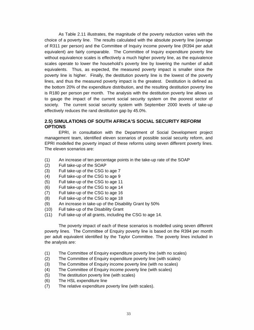
33
As Table 2.11 illustrates, the magnitude of the poverty reduction varies with the choice of a poverty line. The results calculated with the absolute poverty line (average of R311 per person) and the Committee of Inquiry income poverty line (R394 per adult equivalent) are fairly comparable. The Committee of Inquiry expenditure poverty line without equivalence scales is effectively a much higher poverty line, as the equivalence scales operate to lower the household’s poverty line by lowering the number of adult equivalents. Thus, as expected, the measured poverty impact is smaller since the poverty line is higher. Finally, the destitution poverty line is the lowest of the poverty lines, and thus the measured poverty impact is the greatest. Destitution is defined as the bottom 20% of the expenditure distribution, and the resulting destitution poverty line is R180 per person per month. The analysis with the destitution poverty line allows us to gauge the impact of the current social security system on the poorest sector of society. The current social security system with September 2000 levels of take-up effectively reduces the rand destitution gap by 45.0%. 2.5) SIMULATIONS OF SOUTH AFRICA’S SOCIAL SECURITY REFORM OPTIONS EPRI, in consultation with the Department of Social Development project management team, identified eleven scenarios of possible social security reform, and EPRI modelled the poverty impact of these reforms using seven different poverty lines. The eleven scenarios are: (1) An increase of ten percentage points in the take-up rate of the SOAP (2) Full take-up of the SOAP (3) Full take-up of the CSG to age 7 (4) Full take-up of the CSG to age 9 (5) Full take-up of the CSG to age 11 (6) Full take-up of the CSG to age 14 (7) Full take-up of the CSG to age 16 (8) Full take-up of the CSG to age 18 (9) An increase in take-up of the Disability Grant by 50% (10) Full take-up of the Disability Grant (11) Full take-up of all grants, including the CSG to age 14.
The poverty impact of each of these scenarios is modelled using seven different poverty lines. The Committee of Enquiry poverty line is based on the R394 per month per adult equivalent identified by the Taylor Committee. The poverty lines included in the analysis are:
(1) The Committee of Enquiry expenditure poverty line (with no scales) (2) The Committee of Enquiry expenditure poverty line (with scales) (3) The Committee of Enquiry income poverty line (with no scales) (4) The Committee of Enquiry income poverty line (with scales) (5) The destitution poverty line (with scales) (6) The HSL expenditure line (7) The relative expenditure poverty line (with scales).
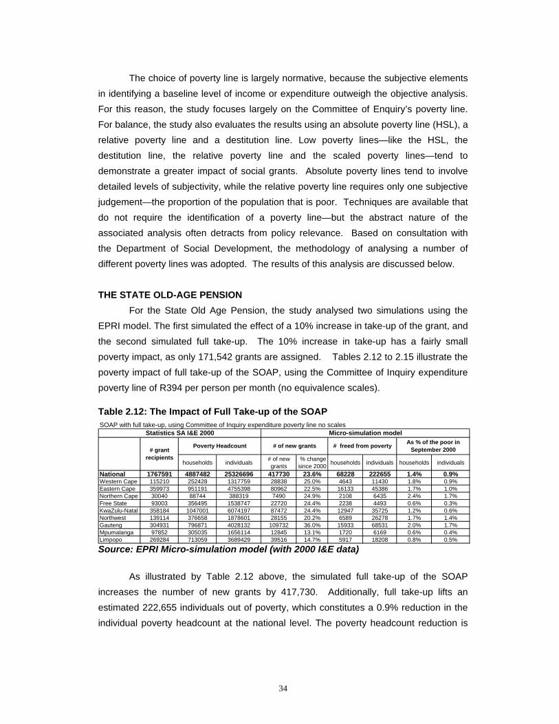
34
The choice of poverty line is largely normative, because the subjective elements in identifying a baseline level of income or expenditure outweigh the objective analysis. For this reason, the study focuses largely on the Committee of Enquiry’s poverty line. For balance, the study also evaluates the results using an absolute poverty line (HSL), a relative poverty line and a destitution line. Low poverty lines—like the HSL, the destitution line, the relative poverty line and the scaled poverty lines—tend to demonstrate a greater impact of social grants. Absolute poverty lines tend to involve detailed levels of subjectivity, while the relative poverty line requires only one subjective judgement—the proportion of the population that is poor. Techniques are available that do not require the identification of a poverty line—but the abstract nature of the associated analysis often detracts from policy relevance. Based on consultation with the Department of Social Development, the methodology of analysing a number of different poverty lines was adopted. The results of this analysis are discussed below. THE STATE OLD-AGE PENSION
For the State Old Age Pension, the study analysed two simulations using the EPRI model. The first simulated the effect of a 10% increase in take-up of the grant, and the second simulated full take-up. The 10% increase in take-up has a fairly small poverty impact, as only 171,542 grants are assigned. Tables 2.12 to 2.15 illustrate the poverty impact of full take-up of the SOAP, using the Committee of Inquiry expenditure poverty line of R394 per person per month (no equivalence scales). Table 2.12: The Impact of Full Take-up of the SOAP
Source: EPRI Micro-simulation model (with 2000 I&E data)
As illustrated by Table 2.12 above, the simulated full take-up of the SOAP increases the number of new grants by 417,730. Additionally, full take-up lifts an estimated 222,655 individuals out of poverty, which constitutes a 0.9% reduction in the individual poverty headcount at the national level. The poverty headcount reduction is
SOAP with full take-up, using Committee of Inquiry expenditure poverty line no scales
households individuals # of new grants
% change since 2000 households individuals households individuals
National 1767591 4887482 25326696 417730 23.6% 68228 222655 1.4% 0.9%Western Cape 115210 252428 1317759 28838 25.0% 4643 11430 1.8% 0.9%Eastern Cape 359973 951191 4755398 80962 22.5% 16133 45386 1.7% 1.0%Northern Cape 30040 88744 388319 7490 24.9% 2108 6435 2.4% 1.7%Free State 93003 356495 1538747 22720 24.4% 2238 4493 0.6% 0.3%KwaZulu-Natal 358184 1047001 6074197 87472 24.4% 12947 35725 1.2% 0.6%Northwest 139114 376658 1878601 28155 20.2% 6589 26278 1.7% 1.4%Gauteng 304931 796871 4028132 109732 36.0% 15933 68531 2.0% 1.7%Mpumalanga 97852 305035 1656114 12845 13.1% 1720 6169 0.6% 0.4%Limpopo 269284 713059 3689429 39516 14.7% 5917 18208 0.8% 0.5%
# of new grants # freed from poverty As % of the poor in September 2000
Micro-simulation modelStatistics SA I&E 2000
Poverty Headcount# grant
recipients
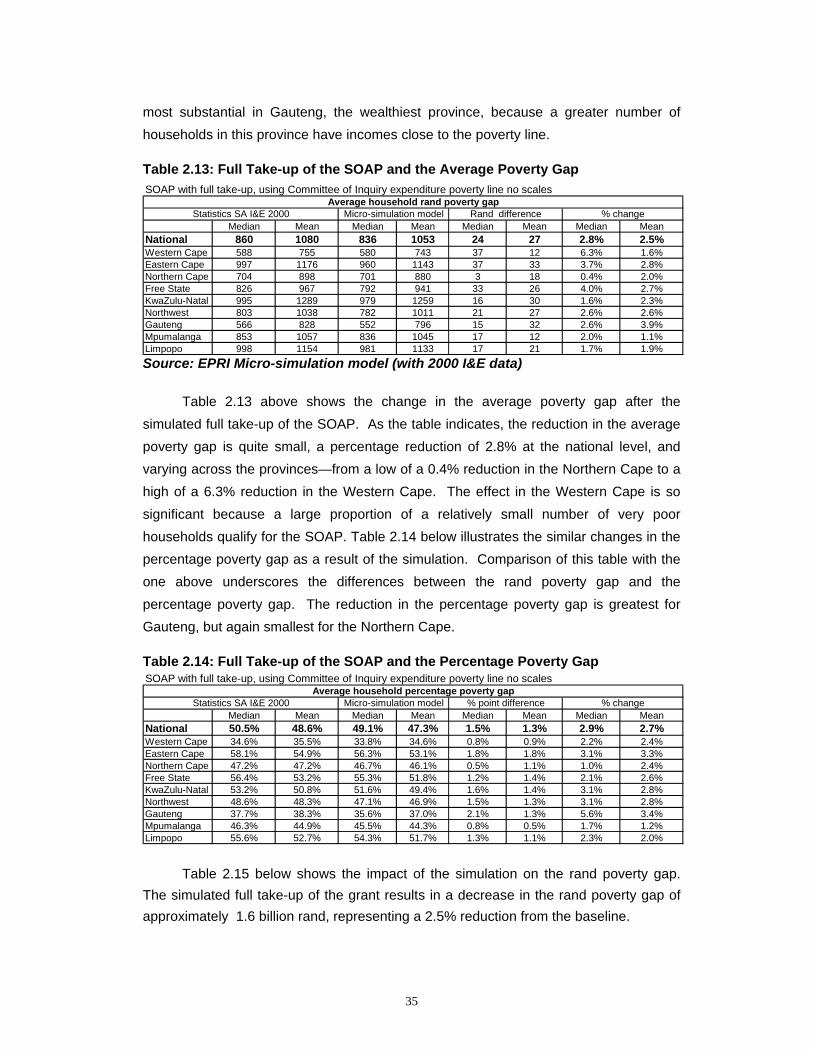
35
most substantial in Gauteng, the wealthiest province, because a greater number of households in this province have incomes close to the poverty line. Table 2.13: Full Take-up of the SOAP and the Average Poverty Gap
Source: EPRI Micro-simulation model (with 2000 I&E data) Table 2.13 above shows the change in the average poverty gap after the simulated full take-up of the SOAP. As the table indicates, the reduction in the average poverty gap is quite small, a percentage reduction of 2.8% at the national level, and varying across the provinces—from a low of a 0.4% reduction in the Northern Cape to a high of a 6.3% reduction in the Western Cape. The effect in the Western Cape is so significant because a large proportion of a relatively small number of very poor households qualify for the SOAP. Table 2.14 below illustrates the similar changes in the percentage poverty gap as a result of the simulation. Comparison of this table with the one above underscores the differences between the rand poverty gap and the percentage poverty gap. The reduction in the percentage poverty gap is greatest for Gauteng, but again smallest for the Northern Cape. Table 2.14: Full Take-up of the SOAP and the Percentage Poverty Gap
Table 2.15 below shows the impact of the simulation on the rand poverty gap. The simulated full take-up of the grant results in a decrease in the rand poverty gap of approximately 1.6 billion rand, representing a 2.5% reduction from the baseline.
SOAP with full take-up, using Committee of Inquiry expenditure poverty line no scales
Median Mean Median Mean Median Mean Median MeanNational 860 1080 836 1053 24 27 2.8% 2.5%Western Cape 588 755 580 743 37 12 6.3% 1.6%Eastern Cape 997 1176 960 1143 37 33 3.7% 2.8%Northern Cape 704 898 701 880 3 18 0.4% 2.0%Free State 826 967 792 941 33 26 4.0% 2.7%KwaZulu-Natal 995 1289 979 1259 16 30 1.6% 2.3%Northwest 803 1038 782 1011 21 27 2.6% 2.6%Gauteng 566 828 552 796 15 32 2.6% 3.9%Mpumalanga 853 1057 836 1045 17 12 2.0% 1.1%Limpopo 998 1154 981 1133 17 21 1.7% 1.9%
Statistics SA I&E 2000 Micro-simulation model Rand differenceAverage household rand poverty gap
% change
SOAP with full take-up, using Committee of Inquiry expenditure poverty line no scales
Median Mean Median Mean Median Mean Median MeanNational 50.5% 48.6% 49.1% 47.3% 1.5% 1.3% 2.9% 2.7%Western Cape 34.6% 35.5% 33.8% 34.6% 0.8% 0.9% 2.2% 2.4%Eastern Cape 58.1% 54.9% 56.3% 53.1% 1.8% 1.8% 3.1% 3.3%Northern Cape 47.2% 47.2% 46.7% 46.1% 0.5% 1.1% 1.0% 2.4%Free State 56.4% 53.2% 55.3% 51.8% 1.2% 1.4% 2.1% 2.6%KwaZulu-Natal 53.2% 50.8% 51.6% 49.4% 1.6% 1.4% 3.1% 2.8%Northwest 48.6% 48.3% 47.1% 46.9% 1.5% 1.3% 3.1% 2.8%Gauteng 37.7% 38.3% 35.6% 37.0% 2.1% 1.3% 5.6% 3.4%Mpumalanga 46.3% 44.9% 45.5% 44.3% 0.8% 0.5% 1.7% 1.2%Limpopo 55.6% 52.7% 54.3% 51.7% 1.3% 1.1% 2.3% 2.0%
% changeStatistics SA I&E 2000 Micro-simulation model % point differenceAverage household percentage poverty gap
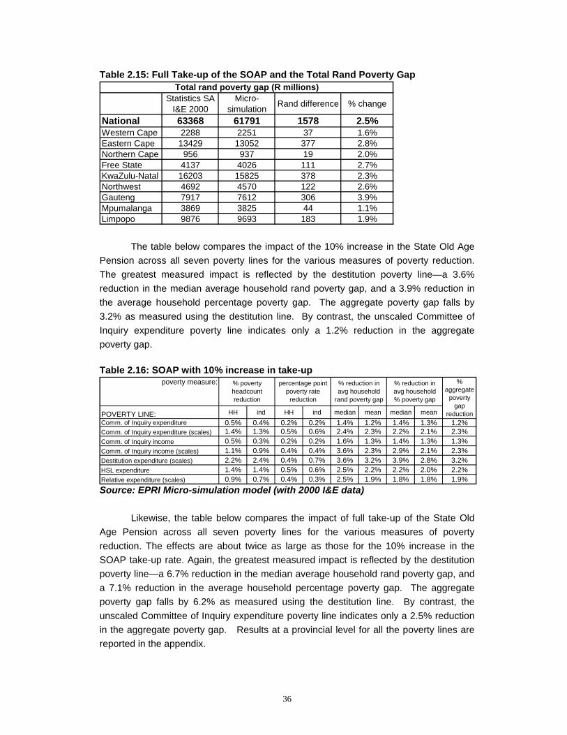
36
Table 2.15: Full Take-up of the SOAP and the Total Rand Poverty Gap
The table below compares the impact of the 10% increase in the State Old Age
Pension across all seven poverty lines for the various measures of poverty reduction. The greatest measured impact is reflected by the destitution poverty line—a 3.6% reduction in the median average household rand poverty gap, and a 3.9% reduction in the average household percentage poverty gap. The aggregate poverty gap falls by 3.2% as measured using the destitution line. By contrast, the unscaled Committee of Inquiry expenditure poverty line indicates only a 1.2% reduction in the aggregate poverty gap. Table 2.16: SOAP with 10% increase in take-up
Source: EPRI Micro-simulation model (with 2000 I&E data)
Likewise, the table below compares the impact of full take-up of the State Old Age Pension across all seven poverty lines for the various measures of poverty reduction. The effects are about twice as large as those for the 10% increase in the SOAP take-up rate. Again, the greatest measured impact is reflected by the destitution poverty line—a 6.7% reduction in the median average household rand poverty gap, and a 7.1% reduction in the average household percentage poverty gap. The aggregate poverty gap falls by 6.2% as measured using the destitution line. By contrast, the unscaled Committee of Inquiry expenditure poverty line indicates only a 2.5% reduction in the aggregate poverty gap. Results at a provincial level for all the poverty lines are reported in the appendix.
poverty measure:
POVERTY LINE: HH ind HH ind median mean median meanComm. of Inquiry expenditure 0.5% 0.4% 0.2% 0.2% 1.4% 1.2% 1.4% 1.3% 1.2%Comm. of Inquiry expenditure (scales) 1.4% 1.3% 0.5% 0.6% 2.4% 2.3% 2.2% 2.1% 2.3%Comm. of Inquiry income 0.5% 0.3% 0.2% 0.2% 1.6% 1.3% 1.4% 1.3% 1.3%Comm. of Inquiry income (scales) 1.1% 0.9% 0.4% 0.4% 3.6% 2.3% 2.9% 2.1% 2.3%Destitution expenditure (scales) 2.2% 2.4% 0.4% 0.7% 3.6% 3.2% 3.9% 2.8% 3.2%HSL expenditure 1.4% 1.4% 0.5% 0.6% 2.5% 2.2% 2.2% 2.0% 2.2%Relative expenditure (scales) 0.9% 0.7% 0.4% 0.3% 2.5% 1.9% 1.8% 1.8% 1.9%
% reduction in avg household % poverty gap
% aggregate
poverty gap
reduction
% poverty headcount reduction
percentage point poverty rate
reduction
% reduction in avg household
rand poverty gap
Statistics SA I&E 2000
Micro-simulation Rand difference % change
National 63368 61791 1578 2.5%Western Cape 2288 2251 37 1.6%Eastern Cape 13429 13052 377 2.8%Northern Cape 956 937 19 2.0%Free State 4137 4026 111 2.7%KwaZulu-Natal 16203 15825 378 2.3%Northwest 4692 4570 122 2.6%Gauteng 7917 7612 306 3.9%Mpumalanga 3869 3825 44 1.1%Limpopo 9876 9693 183 1.9%
Total rand poverty gap (R millions)
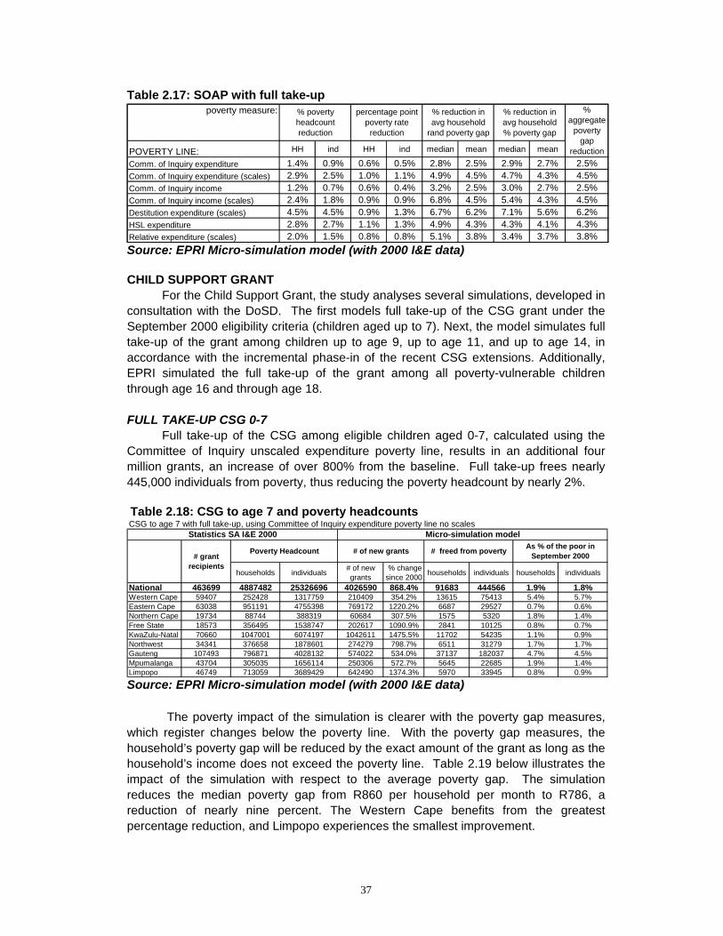
37
Table 2.17: SOAP with full take-up
Source: EPRI Micro-simulation model (with 2000 I&E data) CHILD SUPPORT GRANT For the Child Support Grant, the study analyses several simulations, developed in consultation with the DoSD. The first models full take-up of the CSG grant under the September 2000 eligibility criteria (children aged up to 7). Next, the model simulates full take-up of the grant among children up to age 9, up to age 11, and up to age 14, in accordance with the incremental phase-in of the recent CSG extensions. Additionally, EPRI simulated the full take-up of the grant among all poverty-vulnerable children through age 16 and through age 18. FULL TAKE-UP CSG 0-7 Full take-up of the CSG among eligible children aged 0-7, calculated using the Committee of Inquiry unscaled expenditure poverty line, results in an additional four million grants, an increase of over 800% from the baseline. Full take-up frees nearly 445,000 individuals from poverty, thus reducing the poverty headcount by nearly 2%. Table 2.18: CSG to age 7 and poverty headcounts
Source: EPRI Micro-simulation model (with 2000 I&E data)
The poverty impact of the simulation is clearer with the poverty gap measures, which register changes below the poverty line. With the poverty gap measures, the household’s poverty gap will be reduced by the exact amount of the grant as long as the household’s income does not exceed the poverty line. Table 2.19 below illustrates the impact of the simulation with respect to the average poverty gap. The simulation reduces the median poverty gap from R860 per household per month to R786, a reduction of nearly nine percent. The Western Cape benefits from the greatest percentage reduction, and Limpopo experiences the smallest improvement.
poverty measure:
POVERTY LINE: HH ind HH ind median mean median mean
Comm. of Inquiry expenditure 1.4% 0.9% 0.6% 0.5% 2.8% 2.5% 2.9% 2.7% 2.5%Comm. of Inquiry expenditure (scales) 2.9% 2.5% 1.0% 1.1% 4.9% 4.5% 4.7% 4.3% 4.5%Comm. of Inquiry income 1.2% 0.7% 0.6% 0.4% 3.2% 2.5% 3.0% 2.7% 2.5%Comm. of Inquiry income (scales) 2.4% 1.8% 0.9% 0.9% 6.8% 4.5% 5.4% 4.3% 4.5%Destitution expenditure (scales) 4.5% 4.5% 0.9% 1.3% 6.7% 6.2% 7.1% 5.6% 6.2%HSL expenditure 2.8% 2.7% 1.1% 1.3% 4.9% 4.3% 4.3% 4.1% 4.3%Relative expenditure (scales) 2.0% 1.5% 0.8% 0.8% 5.1% 3.8% 3.4% 3.7% 3.8%
% aggregate
poverty gap
reduction
% poverty headcount reduction
percentage point poverty rate
reduction
% reduction in avg household
rand poverty gap
% reduction in avg household % poverty gap
CSG to age 7 with full take-up, using Committee of Inquiry expenditure poverty line no scales
households individuals # of new grants
% change since 2000 households individuals households individuals
National 463699 4887482 25326696 4026590 868.4% 91683 444566 1.9% 1.8%Western Cape 59407 252428 1317759 210409 354.2% 13615 75413 5.4% 5.7%Eastern Cape 63038 951191 4755398 769172 1220.2% 6687 29527 0.7% 0.6%Northern Cape 19734 88744 388319 60684 307.5% 1575 5320 1.8% 1.4%Free State 18573 356495 1538747 202617 1090.9% 2841 10125 0.8% 0.7%KwaZulu-Natal 70660 1047001 6074197 1042611 1475.5% 11702 54235 1.1% 0.9%Northwest 34341 376658 1878601 274279 798.7% 6511 31279 1.7% 1.7%Gauteng 107493 796871 4028132 574022 534.0% 37137 182037 4.7% 4.5%Mpumalanga 43704 305035 1656114 250306 572.7% 5645 22685 1.9% 1.4%Limpopo 46749 713059 3689429 642490 1374.3% 5970 33945 0.8% 0.9%
# of new grants # freed from poverty As % of the poor in September 2000
Micro-simulation modelStatistics SA I&E 2000
Poverty Headcount# grant
recipients
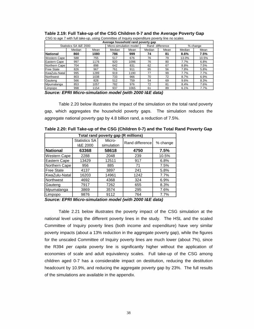
38
Table 2.19: Full Take-up of the CSG Children 0-7 and the Average Poverty Gap
Source: EPRI Micro-simulation model (with 2000 I&E data)
Table 2.20 below illustrates the impact of the simulation on the total rand poverty gap, which aggregates the household poverty gaps. The simulation reduces the aggregate national poverty gap by 4.8 billion rand, a reduction of 7.5%. Table 2.20: Full Take-up of the CSG (Children 0-7) and the Total Rand Poverty Gap
Source: EPRI Micro-simulation model (with 2000 I&E data)
Table 2.21 below illustrates the poverty impact of the CSG simulation at the national level using the different poverty lines in the study. The HSL and the scaled Committee of Inquiry poverty lines (both income and expenditure) have very similar poverty impacts (about a 13% reduction in the aggregate poverty gap), while the figures for the unscaled Committee of Inquiry poverty lines are much lower (about 7%), since the R394 per capita poverty line is significantly higher without the application of economies of scale and adult equivalency scales. Full take-up of the CSG among children aged 0-7 has a considerable impact on destitution, reducing the destitution headcount by 10.9%, and reducing the aggregate poverty gap by 23%. The full results of the simulations are available in the appendix.
CSG to age 7 with full take-up, using Committee of Inquiry expenditure poverty line no scales
Median Mean Median Mean Median Mean Median MeanNational 860 1080 786 999 74 81 8.6% 7.5%Western Cape 588 755 517 676 76 79 13.0% 10.5%Eastern Cape 997 1176 920 1096 76 80 7.7% 6.8%Northern Cape 704 898 642 831 62 67 8.8% 7.5%Free State 826 967 761 911 65 56 7.8% 5.8%KwaZulu-Natal 995 1289 919 1190 77 99 7.7% 7.7%Northwest 803 1038 733 966 70 72 8.7% 6.9%Gauteng 566 828 512 759 54 69 9.6% 8.3%Mpumalanga 853 1057 782 976 72 81 8.4% 7.6%Limpopo 998 1154 937 1065 61 89 6.1% 7.7%
Statistics SA I&E 2000 Micro-simulation model Rand differenceAverage household rand poverty gap
% change
Statistics SA I&E 2000
Micro-simulation Rand difference % change
National 63368 58618 4750 7.5%Western Cape 2288 2048 239 10.5%Eastern Cape 13429 12511 917 6.8%Northern Cape 956 885 71 7.5%Free State 4137 3897 241 5.8%KwaZulu-Natal 16203 14961 1242 7.7%Northwest 4692 4368 324 6.9%Gauteng 7917 7262 655 8.3%Mpumalanga 3869 3574 295 7.6%Limpopo 9876 9112 764 7.7%
Total rand poverty gap (R millions)

39
Table 2.21 CSG to age 7 with full take-up
Source: EPRI Micro-simulation model (with 2000 I&E data)
In addition, the CSG simulations were estimated with increases in the real grant levels to 2003 terms (R1606 per year in 2000 currency units). Table 2.22 below illustrates the poverty impact of this CSG simulation at the national level using the different poverty lines in the study. Again, the HSL and the scaled Committee of Inquiry poverty lines (both income and expenditure) have very similar poverty impacts (a 17-18% reduction in the aggregate poverty gap), while the figures for the unscaled Committee of Inquiry poverty lines are again much lower (about 10%). Full take-up of the higher CSG among children aged 0-7 has a considerable impact on destitution, reducing the destitution headcount by 17.3%, and reducing the aggregate poverty gap by 30.3%. The substantial benefits of the real increase in CSG payments are immediately apparent. The full results of the simulations are available in the appendix. Table 2.22: CSG(1606) to age 7 with full take-up
Source: EPRI Micro-simulation model (with 2000 I&E data) FULL TAKE-UP CSG CHILDREN 0-9 Full take-up of the CSG among eligible children aged 0-9, calculated using the Committee of Inquiry unscaled expenditure poverty line, results in more than five million additional grants, an increase of nearly 1200% from the baseline. Full take-up frees more than 624,000 individuals from poverty (180,000 more than with the CSG from 0-7), thus reducing the poverty headcount by 2.5%.
poverty measure:
POVERTY LINE: HH ind HH ind median mean median mean
Comm. of Inquiry expenditure 1.9% 1.8% 0.8% 1.0% 8.6% 7.5% 6.8% 7.0% 7.5%Comm. of Inquiry expenditure (scales) 5.1% 5.3% 1.8% 2.5% 16.4% 13.4% 13.5% 12.4% 13.4%Comm. of Inquiry income 1.4% 1.4% 0.7% 0.8% 8.7% 7.4% 7.2% 6.9% 7.4%Comm. of Inquiry income (scales) 4.2% 4.2% 1.6% 2.1% 15.8% 13.3% 15.1% 12.4% 13.3%Destitution expenditure (scales) 11.1% 10.9% 2.2% 3.4% 28.2% 23.0% 25.6% 21.4% 23.0%HSL expenditure 4.8% 5.8% 1.9% 2.7% 13.2% 13.0% 13.0% 11.3% 13.0%Relative expenditure (scales) 3.8% 3.9% 1.5% 2.0% 12.4% 10.7% 10.6% 9.9% 10.7%
% poverty headcount reduction
percentage point poverty rate
reduction
% reduction in avg household
rand poverty gap
% reduction in avg household % poverty gap
% aggregate
poverty gap
reduction
poverty measure:
POVERTY LINE: HH ind HH ind median mean median mean
Comm. of Inquiry expenditure 2.6% 2.3% 1.1% 1.4% 11.3% 10.0% 8.9% 9.3% 10.0%Comm. of Inquiry expenditure (scales) 7.0% 7.4% 2.4% 3.4% 21.8% 17.6% 18.1% 16.1% 17.6%Comm. of Inquiry income 1.9% 1.8% 0.9% 1.1% 11.5% 9.8% 10.0% 9.2% 9.8%Comm. of Inquiry income (scales) 5.6% 5.7% 2.1% 2.8% 22.6% 17.4% 20.9% 16.2% 17.4%Destitution expenditure (scales) 17.3% 19.6% 3.5% 5.7% 36.8% 30.3% 33.2% 27.1% 30.3%HSL expenditure 6.5% 8.0% 2.5% 3.7% 18.0% 17.0% 17.3% 14.8% 17.0%Relative expenditure (scales) 5.0% 5.3% 2.0% 2.8% 16.0% 14.1% 14.1% 13.0% 14.1%
% poverty headcount reduction
percentage point poverty rate
reduction
% reduction in avg household
rand poverty gap
% reduction in avg household % poverty gap
% aggregate
poverty gap
reduction

40
Table 2.23: CSG to age 9 and poverty headcounts
Source: EPRI Micro-simulation model (with 2000 I&E data)
Table 2.24 below illustrates the poverty impact of the CSG simulation to age 9 at the national level using the different poverty lines in the study. The HSL and the scaled Committee of Inquiry poverty lines (both income and expenditure) again have very similar poverty impacts (a 17-18% reduction in the aggregate poverty gap), while the figures for the unscaled Committee of Inquiry poverty lines are still much lower (about 10%). Full take-up of the CSG among children aged 0-9 has a considerable impact on destitution, reducing the destitution headcount by 15.6%, and reducing the aggregate poverty gap by 30%. The full results of the simulations are available in the appendix. Table 2.24: CSG to age 9 with full take-up
Source: EPRI Micro-simulation model (with 2000 I&E data)
Again, the CSG simulations were estimated with increases in the real grant levels to 2003 terms. Table 2.25 below illustrates the poverty impact of this CSG simulation at the national level using the different poverty lines in the study. The HSL and the scaled Committee of Inquiry poverty lines have very similar poverty impacts (a 23% reduction in the aggregate poverty gap), while the figures for the unscaled Committee of Inquiry poverty lines are still much lower (about 13%). Full take-up of the higher CSG among children aged 0-9 has a considerable impact on destitution, reducing the destitution headcount by 25.9%, and reducing the aggregate poverty gap (destitution gap) by 39.2%. Again, the substantial benefits of the real increase in CSG payments are immediately apparent. The full results of the simulations are available in the appendix.
poverty measure:
POVERTY LINE: HH ind HH ind median mean median mean
Comm. of Inquiry expenditure 2.6% 2.5% 1.1% 1.5% 11.1% 10.1% 9.1% 9.5% 10.1%Comm. of Inquiry expenditure (scales) 7.3% 7.7% 2.5% 3.6% 21.1% 17.9% 17.5% 16.6% 17.9%Comm. of Inquiry income 1.9% 1.8% 0.9% 1.1% 11.5% 9.9% 9.9% 9.4% 9.9%Comm. of Inquiry income (scales) 5.8% 6.0% 2.2% 3.0% 22.4% 17.7% 21.0% 16.6% 17.7%Destitution expenditure (scales) 15.9% 15.6% 3.2% 4.9% 36.8% 30.3% 34.8% 28.4% 30.3%HSL expenditure 6.3% 7.6% 2.4% 3.6% 17.9% 17.4% 17.0% 15.2% 17.4%Relative expenditure (scales) 5.0% 5.2% 2.0% 2.7% 16.8% 14.3% 14.3% 13.3% 14.3%
% aggregate
poverty gap
reduction
% poverty headcount reduction
percentage point poverty rate
reduction
% reduction in avg household
rand poverty gap
% reduction in avg household % poverty gap
CSG to age 9 with full take-up, using Committee of Inquiry expenditure poverty line no scales
households individuals # of new grants
% change since 2000 households individuals households individuals
National 463699 4887482 25326696 5413470 1167.5% 124703 624262 2.6% 2.5%Western Cape 59407 252428 1317759 274483 462.0% 15551 87513 6.2% 6.6%Eastern Cape 63038 951191 4755398 1045120 1657.9% 11160 48705 1.2% 1.0%Northern Cape 19734 88744 388319 77530 392.9% 2563 8840 2.9% 2.3%Free State 18573 356495 1538747 278621 1500.1% 4161 18157 1.2% 1.2%KwaZulu-Natal 70660 1047001 6074197 1403055 1985.6% 15216 73066 1.5% 1.2%Northwest 34341 376658 1878601 372722 1085.4% 10084 47984 2.7% 2.6%Gauteng 107493 796871 4028132 755032 702.4% 47156 248945 5.9% 6.2%Mpumalanga 43704 305035 1656114 346442 792.7% 7401 30952 2.4% 1.9%Limpopo 46749 713059 3689429 860465 1840.6% 11411 60100 1.6% 1.6%
# of new grants # freed from poverty As % of the poor in September 2000
Micro-simulation modelStatistics SA I&E 2000
Poverty Headcount# grant
recipients
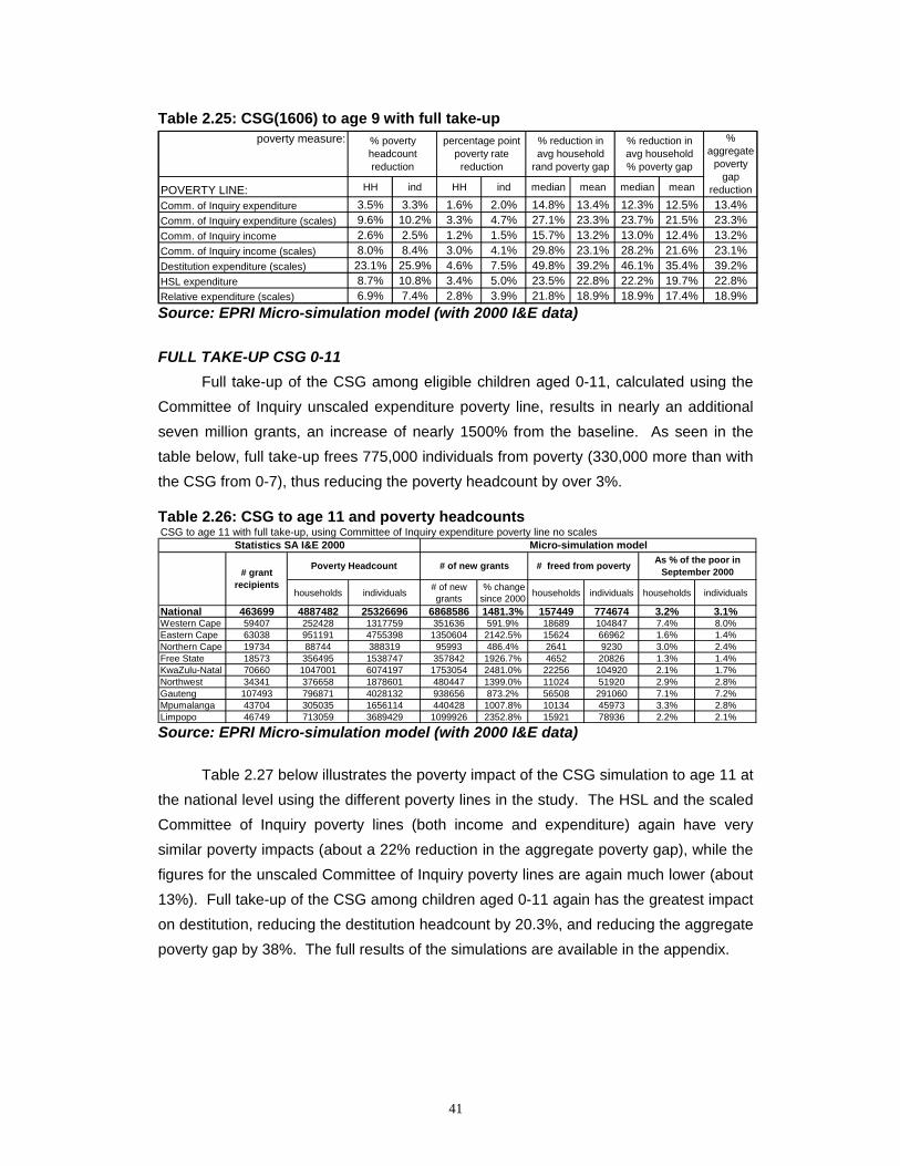
41
Table 2.25: CSG(1606) to age 9 with full take-up
Source: EPRI Micro-simulation model (with 2000 I&E data) FULL TAKE-UP CSG 0-11 Full take-up of the CSG among eligible children aged 0-11, calculated using the Committee of Inquiry unscaled expenditure poverty line, results in nearly an additional seven million grants, an increase of nearly 1500% from the baseline. As seen in the table below, full take-up frees 775,000 individuals from poverty (330,000 more than with the CSG from 0-7), thus reducing the poverty headcount by over 3%. Table 2.26: CSG to age 11 and poverty headcounts
Source: EPRI Micro-simulation model (with 2000 I&E data) Table 2.27 below illustrates the poverty impact of the CSG simulation to age 11 at the national level using the different poverty lines in the study. The HSL and the scaled Committee of Inquiry poverty lines (both income and expenditure) again have very similar poverty impacts (about a 22% reduction in the aggregate poverty gap), while the figures for the unscaled Committee of Inquiry poverty lines are again much lower (about 13%). Full take-up of the CSG among children aged 0-11 again has the greatest impact on destitution, reducing the destitution headcount by 20.3%, and reducing the aggregate poverty gap by 38%. The full results of the simulations are available in the appendix.
poverty measure:
POVERTY LINE: HH ind HH ind median mean median mean
Comm. of Inquiry expenditure 3.5% 3.3% 1.6% 2.0% 14.8% 13.4% 12.3% 12.5% 13.4%Comm. of Inquiry expenditure (scales) 9.6% 10.2% 3.3% 4.7% 27.1% 23.3% 23.7% 21.5% 23.3%Comm. of Inquiry income 2.6% 2.5% 1.2% 1.5% 15.7% 13.2% 13.0% 12.4% 13.2%Comm. of Inquiry income (scales) 8.0% 8.4% 3.0% 4.1% 29.8% 23.1% 28.2% 21.6% 23.1%Destitution expenditure (scales) 23.1% 25.9% 4.6% 7.5% 49.8% 39.2% 46.1% 35.4% 39.2%HSL expenditure 8.7% 10.8% 3.4% 5.0% 23.5% 22.8% 22.2% 19.7% 22.8%Relative expenditure (scales) 6.9% 7.4% 2.8% 3.9% 21.8% 18.9% 18.9% 17.4% 18.9%
% aggregate
poverty gap
reduction
% poverty headcount reduction
percentage point poverty rate
reduction
% reduction in avg household
rand poverty gap
% reduction in avg household % poverty gap
CSG to age 11 with full take-up, using Committee of Inquiry expenditure poverty line no scales
households individuals # of new grants
% change since 2000 households individuals households individuals
National 463699 4887482 25326696 6868586 1481.3% 157449 774674 3.2% 3.1%Western Cape 59407 252428 1317759 351636 591.9% 18689 104847 7.4% 8.0%Eastern Cape 63038 951191 4755398 1350604 2142.5% 15624 66962 1.6% 1.4%Northern Cape 19734 88744 388319 95993 486.4% 2641 9230 3.0% 2.4%Free State 18573 356495 1538747 357842 1926.7% 4652 20826 1.3% 1.4%KwaZulu-Natal 70660 1047001 6074197 1753054 2481.0% 22256 104920 2.1% 1.7%Northwest 34341 376658 1878601 480447 1399.0% 11024 51920 2.9% 2.8%Gauteng 107493 796871 4028132 938656 873.2% 56508 291060 7.1% 7.2%Mpumalanga 43704 305035 1656114 440428 1007.8% 10134 45973 3.3% 2.8%Limpopo 46749 713059 3689429 1099926 2352.8% 15921 78936 2.2% 2.1%
# of new grants # freed from poverty As % of the poor in September 2000
Micro-simulation modelStatistics SA I&E 2000
Poverty Headcount# grant
recipients
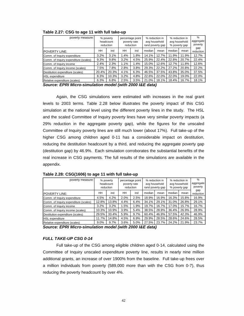
42
Table 2.27: CSG to age 11 with full take-up
Source: EPRI Micro-simulation model (with 2000 I&E data)
Again, the CSG simulations were estimated with increases in the real grant levels to 2003 terms. Table 2.28 below illustrates the poverty impact of this CSG simulation at the national level using the different poverty lines in the study. The HSL and the scaled Committee of Inquiry poverty lines have very similar poverty impacts (a 29% reduction in the aggregate poverty gap), while the figures for the unscaled Committee of Inquiry poverty lines are still much lower (about 17%). Full take-up of the higher CSG among children aged 0-11 has a considerable impact on destitution, reducing the destitution headcount by a third, and reducing the aggregate poverty gap (destitution gap) by 46.9%. Each simulation corroborates the substantial benefits of the real increase in CSG payments. The full results of the simulations are available in the appendix. Table 2.28: CSG(1606) to age 11 with full take-up
Source: EPRI Micro-simulation model (with 2000 I&E data) FULL TAKE-UP CSG 0-14
Full take-up of the CSG among eligible children aged 0-14, calculated using the Committee of Inquiry unscaled expenditure poverty line, results in nearly nine million additional grants, an increase of over 1900% from the baseline. Full take-up frees over a million individuals from poverty (589,000 more than with the CSG from 0-7), thus reducing the poverty headcount by over 4%.
poverty measure:
POVERTY LINE: HH ind HH ind median mean median mean
Comm. of Inquiry expenditure 3.2% 3.1% 1.4% 1.8% 14.1% 12.7% 11.9% 11.9% 12.7%Comm. of Inquiry expenditure (scales) 9.3% 9.8% 3.2% 4.5% 25.9% 22.4% 22.8% 20.7% 22.4%Comm. of Inquiry income 2.4% 2.3% 1.1% 1.4% 15.0% 12.6% 12.7% 11.8% 12.6%Comm. of Inquiry income (scales) 7.5% 7.8% 2.8% 3.8% 29.3% 22.2% 27.2% 20.8% 22.2%Destitution expenditure (scales) 20.4% 20.3% 4.1% 6.3% 46.5% 37.5% 43.8% 35.0% 37.5%HSL expenditure 8.3% 10.3% 3.2% 4.8% 22.6% 22.0% 22.0% 19.0% 22.0%Relative expenditure (scales) 6.3% 6.8% 2.5% 3.5% 21.0% 18.1% 18.4% 16.7% 18.1%
% poverty headcount reduction
percentage point poverty rate
reduction
% reduction in avg household
rand poverty gap
% reduction in avg household % poverty gap
% aggregate
poverty gap
reduction
poverty measure:
POVERTY LINE: HH ind HH ind median mean median mean
Comm. of Inquiry expenditure 4.5% 4.2% 2.0% 2.5% 18.9% 16.9% 16.3% 15.8% 16.9%Comm. of Inquiry expenditure (scales) 12.8% 13.8% 4.4% 6.4% 34.1% 29.1% 31.0% 26.8% 29.1%Comm. of Inquiry income 3.2% 3.2% 1.5% 1.9% 19.7% 16.7% 17.0% 15.7% 16.7%Comm. of Inquiry income (scales) 10.3% 10.9% 3.9% 5.4% 38.5% 28.9% 36.4% 26.9% 28.9%Destitution expenditure (scales) 29.5% 33.4% 5.9% 9.7% 60.4% 46.9% 57.5% 42.3% 46.9%HSL expenditure 11.7% 14.8% 4.5% 6.9% 29.9% 28.5% 28.6% 24.6% 28.5%Relative expenditure (scales) 9.0% 9.7% 3.6% 5.0% 27.5% 23.7% 24.2% 21.9% 23.7%
% poverty headcount reduction
percentage point poverty rate
reduction
% reduction in avg household
rand poverty gap
% reduction in avg household % poverty gap
% aggregate
poverty gap
reduction
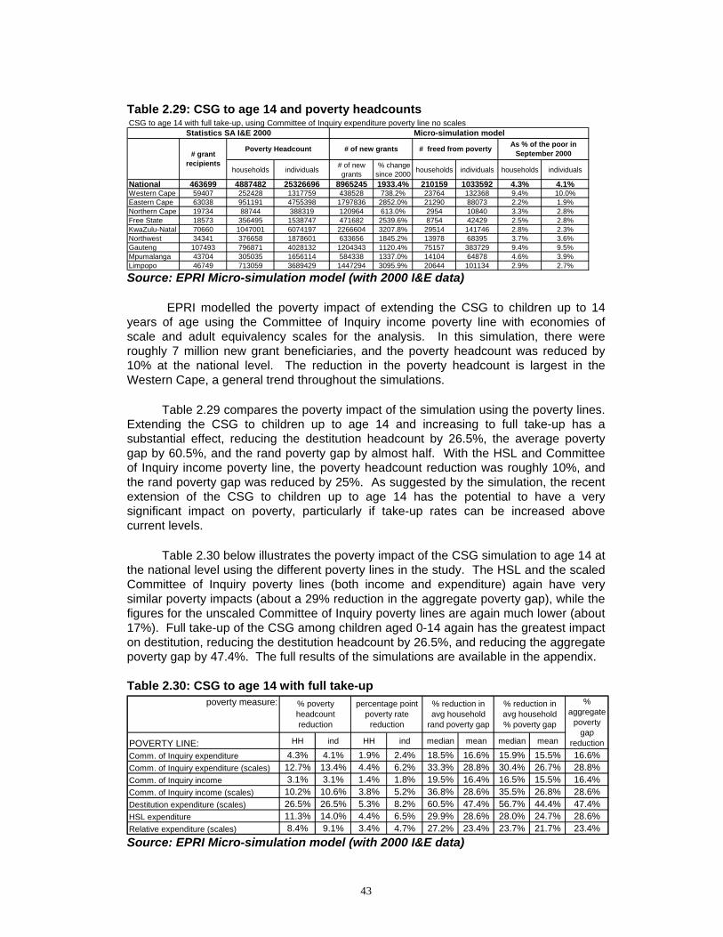
43
Table 2.29: CSG to age 14 and poverty headcounts
Source: EPRI Micro-simulation model (with 2000 I&E data)
EPRI modelled the poverty impact of extending the CSG to children up to 14 years of age using the Committee of Inquiry income poverty line with economies of scale and adult equivalency scales for the analysis. In this simulation, there were roughly 7 million new grant beneficiaries, and the poverty headcount was reduced by 10% at the national level. The reduction in the poverty headcount is largest in the Western Cape, a general trend throughout the simulations. Table 2.29 compares the poverty impact of the simulation using the poverty lines. Extending the CSG to children up to age 14 and increasing to full take-up has a substantial effect, reducing the destitution headcount by 26.5%, the average poverty gap by 60.5%, and the rand poverty gap by almost half. With the HSL and Committee of Inquiry income poverty line, the poverty headcount reduction was roughly 10%, and the rand poverty gap was reduced by 25%. As suggested by the simulation, the recent extension of the CSG to children up to age 14 has the potential to have a very significant impact on poverty, particularly if take-up rates can be increased above current levels. Table 2.30 below illustrates the poverty impact of the CSG simulation to age 14 at the national level using the different poverty lines in the study. The HSL and the scaled Committee of Inquiry poverty lines (both income and expenditure) again have very similar poverty impacts (about a 29% reduction in the aggregate poverty gap), while the figures for the unscaled Committee of Inquiry poverty lines are again much lower (about 17%). Full take-up of the CSG among children aged 0-14 again has the greatest impact on destitution, reducing the destitution headcount by 26.5%, and reducing the aggregate poverty gap by 47.4%. The full results of the simulations are available in the appendix. Table 2.30: CSG to age 14 with full take-up
Source: EPRI Micro-simulation model (with 2000 I&E data)
poverty measure:
POVERTY LINE: HH ind HH ind median mean median mean
Comm. of Inquiry expenditure 4.3% 4.1% 1.9% 2.4% 18.5% 16.6% 15.9% 15.5% 16.6%Comm. of Inquiry expenditure (scales) 12.7% 13.4% 4.4% 6.2% 33.3% 28.8% 30.4% 26.7% 28.8%Comm. of Inquiry income 3.1% 3.1% 1.4% 1.8% 19.5% 16.4% 16.5% 15.5% 16.4%Comm. of Inquiry income (scales) 10.2% 10.6% 3.8% 5.2% 36.8% 28.6% 35.5% 26.8% 28.6%Destitution expenditure (scales) 26.5% 26.5% 5.3% 8.2% 60.5% 47.4% 56.7% 44.4% 47.4%HSL expenditure 11.3% 14.0% 4.4% 6.5% 29.9% 28.6% 28.0% 24.7% 28.6%Relative expenditure (scales) 8.4% 9.1% 3.4% 4.7% 27.2% 23.4% 23.7% 21.7% 23.4%
% aggregate
poverty gap
reduction
% poverty headcount reduction
percentage point poverty rate
reduction
% reduction in avg household
rand poverty gap
% reduction in avg household % poverty gap
CSG to age 14 with full take-up, using Committee of Inquiry expenditure poverty line no scales
households individuals # of new grants
% change since 2000 households individuals households individuals
National 463699 4887482 25326696 8965245 1933.4% 210159 1033592 4.3% 4.1%Western Cape 59407 252428 1317759 438528 738.2% 23764 132368 9.4% 10.0%Eastern Cape 63038 951191 4755398 1797836 2852.0% 21290 88073 2.2% 1.9%Northern Cape 19734 88744 388319 120964 613.0% 2954 10840 3.3% 2.8%Free State 18573 356495 1538747 471682 2539.6% 8754 42429 2.5% 2.8%KwaZulu-Natal 70660 1047001 6074197 2266604 3207.8% 29514 141746 2.8% 2.3%Northwest 34341 376658 1878601 633656 1845.2% 13978 68395 3.7% 3.6%Gauteng 107493 796871 4028132 1204343 1120.4% 75157 383729 9.4% 9.5%Mpumalanga 43704 305035 1656114 584338 1337.0% 14104 64878 4.6% 3.9%Limpopo 46749 713059 3689429 1447294 3095.9% 20644 101134 2.9% 2.7%
# of new grants # freed from poverty As % of the poor in September 2000
Micro-simulation modelStatistics SA I&E 2000
Poverty Headcount# grant
recipients
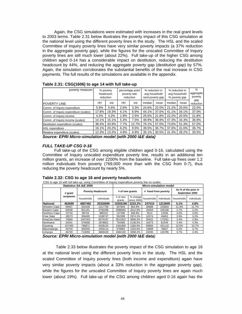
44
Again, the CSG simulations were estimated with increases in the real grant levels to 2003 terms. Table 2.31 below illustrates the poverty impact of this CSG simulation at the national level using the different poverty lines in the study. The HSL and the scaled Committee of Inquiry poverty lines have very similar poverty impacts (a 37% reduction in the aggregate poverty gap), while the figures for the unscaled Committee of Inquiry poverty lines are still much lower (about 22%). Full take-up of the higher CSG among children aged 0-14 has a considerable impact on destitution, reducing the destitution headcount by 44%, and reducing the aggregate poverty gap (destitution gap) by 57%. Again, the simulation corroborates the substantial benefits of the real increase in CSG payments. The full results of the simulations are available in the appendix. Table 2.31: CSG(1606) to age 14 with full take-up
Source: EPRI Micro-simulation model (with 2000 I&E data) FULL TAKE-UP CSG 0-16 Full take-up of the CSG among eligible children aged 0-16, calculated using the Committee of Inquiry unscaled expenditure poverty line, results in an additional ten million grants, an increase of over 2200% from the baseline. Full take-up frees over 1.2 million individuals from poverty (769,000 more than with the CSG from 0-7), thus reducing the poverty headcount by nearly 5%. Table 2.32: CSG to age 16 and poverty headcounts
Source: EPRI Micro-simulation model (with 2000 I&E data)
Table 2.33 below illustrates the poverty impact of the CSG simulation to age 16 at the national level using the different poverty lines in the study. The HSL and the scaled Committee of Inquiry poverty lines (both income and expenditure) again have very similar poverty impacts (about a 33% reduction in the aggregate poverty gap), while the figures for the unscaled Committee of Inquiry poverty lines are again much lower (about 19%). Full take-up of the CSG among children aged 0-16 again has the
poverty measure:
POVERTY LINE: HH ind HH ind median mean median mean
Comm. of Inquiry expenditure 5.9% 5.6% 2.6% 3.3% 24.6% 22.0% 21.2% 20.6% 22.0%Comm. of Inquiry expenditure (scales) 17.8% 19.3% 6.1% 8.9% 44.1% 37.0% 41.1% 34.1% 37.0%Comm. of Inquiry income 4.2% 4.2% 1.9% 2.5% 25.6% 21.8% 22.2% 20.5% 21.8%Comm. of Inquiry income (scales) 14.1% 15.1% 5.3% 7.5% 48.9% 36.9% 47.3% 34.3% 36.9%Destitution expenditure (scales) 38.4% 43.9% 7.7% 12.7% 76.1% 57.0% 73.6% 51.3% 57.0%HSL expenditure 16.1% 20.2% 6.2% 9.5% 39.5% 36.7% 37.6% 31.6% 36.7%Relative expenditure (scales) 12.3% 13.2% 4.9% 6.9% 35.1% 30.5% 31.3% 28.2% 30.5%
% aggregate
poverty gap
reduction
% poverty headcount reduction
percentage point poverty rate
reduction
% reduction in avg household
rand poverty gap
% reduction in avg household % poverty gap
CSG to age 16 with full take-up, using Committee of Inquiry expenditure poverty line no scales
households individuals # of new grants
% change since 2000 households individuals households individuals
National 463699 4887482 25326696 10355186 2233.2% 247015 1213609 5.1% 4.8%Western Cape 59407 252428 1317759 507844 854.9% 28688 153664 11.4% 11.7%Eastern Cape 63038 951191 4755398 2088364 3312.9% 25453 105108 2.7% 2.2%Northern Cape 19734 88744 388319 137499 696.8% 3514 14036 4.0% 3.6%Free State 18573 356495 1538747 552399 2974.2% 10374 49453 2.9% 3.2%KwaZulu-Natal 70660 1047001 6074197 2611822 3696.3% 35422 173261 3.4% 2.9%Northwest 34341 376658 1878601 734366 2138.5% 16573 81549 4.4% 4.3%Gauteng 107493 796871 4028132 1361809 1266.9% 83893 431116 10.5% 10.7%Mpumalanga 43704 305035 1656114 678983 1553.6% 16808 78637 5.5% 4.7%Limpopo 46749 713059 3689429 1682100 3598.2% 26290 126785 3.7% 3.4%
# of new grants # freed from poverty As % of the poor in September 2000
Micro-simulation modelStatistics SA I&E 2000
Poverty Headcount# grant
recipients
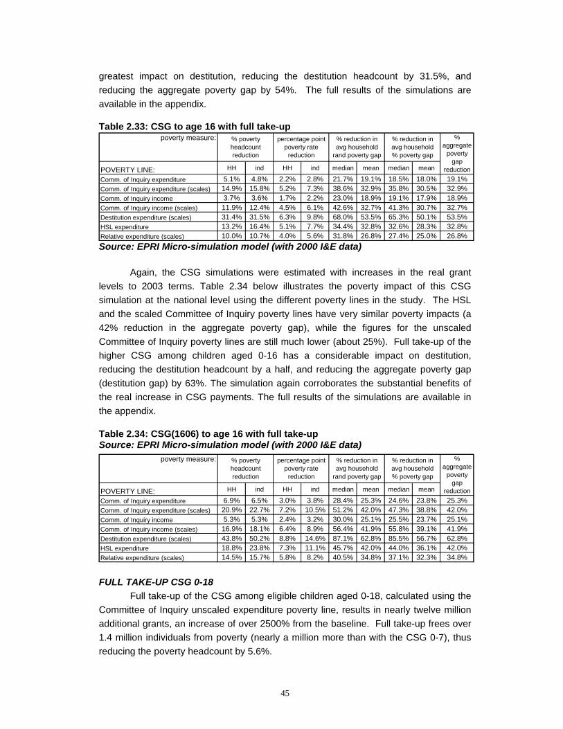
45
greatest impact on destitution, reducing the destitution headcount by 31.5%, and reducing the aggregate poverty gap by 54%. The full results of the simulations are available in the appendix. Table 2.33: CSG to age 16 with full take-up
Source: EPRI Micro-simulation model (with 2000 I&E data)
Again, the CSG simulations were estimated with increases in the real grant levels to 2003 terms. Table 2.34 below illustrates the poverty impact of this CSG simulation at the national level using the different poverty lines in the study. The HSL and the scaled Committee of Inquiry poverty lines have very similar poverty impacts (a 42% reduction in the aggregate poverty gap), while the figures for the unscaled Committee of Inquiry poverty lines are still much lower (about 25%). Full take-up of the higher CSG among children aged 0-16 has a considerable impact on destitution, reducing the destitution headcount by a half, and reducing the aggregate poverty gap (destitution gap) by 63%. The simulation again corroborates the substantial benefits of the real increase in CSG payments. The full results of the simulations are available in the appendix. Table 2.34: CSG(1606) to age 16 with full take-up Source: EPRI Micro-simulation model (with 2000 I&E data)
FULL TAKE-UP CSG 0-18
Full take-up of the CSG among eligible children aged 0-18, calculated using the Committee of Inquiry unscaled expenditure poverty line, results in nearly twelve million additional grants, an increase of over 2500% from the baseline. Full take-up frees over 1.4 million individuals from poverty (nearly a million more than with the CSG 0-7), thus reducing the poverty headcount by 5.6%.
poverty measure:
POVERTY LINE: HH ind HH ind median mean median mean
Comm. of Inquiry expenditure 5.1% 4.8% 2.2% 2.8% 21.7% 19.1% 18.5% 18.0% 19.1%Comm. of Inquiry expenditure (scales) 14.9% 15.8% 5.2% 7.3% 38.6% 32.9% 35.8% 30.5% 32.9%Comm. of Inquiry income 3.7% 3.6% 1.7% 2.2% 23.0% 18.9% 19.1% 17.9% 18.9%Comm. of Inquiry income (scales) 11.9% 12.4% 4.5% 6.1% 42.6% 32.7% 41.3% 30.7% 32.7%Destitution expenditure (scales) 31.4% 31.5% 6.3% 9.8% 68.0% 53.5% 65.3% 50.1% 53.5%HSL expenditure 13.2% 16.4% 5.1% 7.7% 34.4% 32.8% 32.6% 28.3% 32.8%Relative expenditure (scales) 10.0% 10.7% 4.0% 5.6% 31.8% 26.8% 27.4% 25.0% 26.8%
% poverty headcount reduction
percentage point poverty rate
reduction
% reduction in avg household
rand poverty gap
% reduction in avg household % poverty gap
% aggregate
poverty gap
reduction
poverty measure:
POVERTY LINE: HH ind HH ind median mean median mean
Comm. of Inquiry expenditure 6.9% 6.5% 3.0% 3.8% 28.4% 25.3% 24.6% 23.8% 25.3%Comm. of Inquiry expenditure (scales) 20.9% 22.7% 7.2% 10.5% 51.2% 42.0% 47.3% 38.8% 42.0%Comm. of Inquiry income 5.3% 5.3% 2.4% 3.2% 30.0% 25.1% 25.5% 23.7% 25.1%Comm. of Inquiry income (scales) 16.9% 18.1% 6.4% 8.9% 56.4% 41.9% 55.8% 39.1% 41.9%Destitution expenditure (scales) 43.8% 50.2% 8.8% 14.6% 87.1% 62.8% 85.5% 56.7% 62.8%HSL expenditure 18.8% 23.8% 7.3% 11.1% 45.7% 42.0% 44.0% 36.1% 42.0%Relative expenditure (scales) 14.5% 15.7% 5.8% 8.2% 40.5% 34.8% 37.1% 32.3% 34.8%
% poverty headcount reduction
percentage point poverty rate
reduction
% reduction in avg household
rand poverty gap
% reduction in avg household % poverty gap
% aggregate
poverty gap
reduction
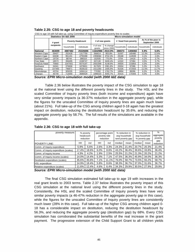
46
Table 2.35: CSG to age 18 and poverty headcounts
Source: EPRI Micro-simulation model (with 2000 I&E data)
Table 2.36 below illustrates the poverty impact of the CSG simulation to age 18 at the national level using the different poverty lines in the study. The HSL and the scaled Committee of Inquiry poverty lines (both income and expenditure) again have very similar poverty impacts (a 36-37% reduction in the aggregate poverty gap), while the figures for the unscaled Committee of Inquiry poverty lines are again much lower (about 21%). Full take-up of the CSG among children aged 0-18 again has the greatest impact on destitution, reducing the destitution headcount by 35.6%, and reducing the aggregate poverty gap by 58.7%. The full results of the simulations are available in the appendix. Table 2.36: CSG to age 18 with full take-up
Source: EPRI Micro-simulation model (with 2000 I&E data)
The final CSG simulation estimated full take-up to age 19 with increases in the real grant levels to 2003 terms. Table 2.37 below illustrates the poverty impact of this CSG simulation at the national level using the different poverty lines in the study. Consistently, the HSL and the scaled Committee of Inquiry poverty lines have very similar poverty impacts (a 46-47% reduction in the aggregate poverty gap in this case), while the figures for the unscaled Committee of Inquiry poverty lines are consistently much lower (28% in this case). Full take-up of the higher CSG among children aged 0-18 has a considerable impact on destitution, reducing the destitution headcount by 56.3%, and reducing the aggregate poverty gap (destitution gap) by 68%. Every CSG simulation has corroborated the substantial benefits of the real increase in the grant payment. The progressive extension of the Child Support Grant to all children yields
poverty measure:
POVERTY LINE: HH ind HH ind median mean median mean
Comm. of Inquiry expenditure 5.9% 5.6% 2.6% 3.3% 24.3% 21.4% 20.7% 20.3% 21.4%Comm. of Inquiry expenditure (scales) 17.4% 18.6% 6.0% 8.6% 43.2% 36.4% 39.6% 33.8% 36.4%Comm. of Inquiry income 4.3% 4.2% 1.9% 2.5% 25.5% 21.2% 21.3% 20.2% 21.2%Comm. of Inquiry income (scales) 14.0% 14.4% 5.3% 7.1% 47.5% 36.3% 45.9% 34.0% 36.3%Destitution expenditure (scales) 35.6% 35.6% 7.1% 11.1% 76.0% 58.7% 73.5% 55.2% 58.7%HSL expenditure 14.9% 18.4% 5.8% 8.6% 38.3% 36.7% 37.0% 31.6% 36.7%Relative expenditure (scales) 11.6% 12.4% 4.6% 6.4% 34.3% 29.9% 30.5% 27.9% 29.9%
% aggregate
poverty gap
reduction
% poverty headcount reduction
percentage point poverty rate
reduction
% reduction in avg household
rand poverty gap
% reduction in avg household % poverty gap
CSG to age 18 with full take-up, using Committee of Inquiry expenditure poverty line no scales
households individuals # of new grants
% change since 2000 households individuals households individuals
National 463699 4887482 25326696 11642986 2510.9% 286573 1406082 5.9% 5.6%Western Cape 59407 252428 1317759 566614 953.8% 31007 165480 12.3% 12.6%Eastern Cape 63038 951191 4755398 2359084 3742.3% 29188 124539 3.1% 2.6%Northern Cape 19734 88744 388319 152935 775.0% 3704 14416 4.2% 3.7%Free State 18573 356495 1538747 637130 3430.4% 12322 57084 3.5% 3.7%KwaZulu-Natal 70660 1047001 6074197 2931599 4148.9% 44504 215853 4.3% 3.6%Northwest 34341 376658 1878601 817929 2381.8% 20004 97086 5.3% 5.2%Gauteng 107493 796871 4028132 1511283 1405.9% 91535 472933 11.5% 11.7%Mpumalanga 43704 305035 1656114 770392 1762.7% 18894 88286 6.2% 5.3%Limpopo 46749 713059 3689429 1896020 4055.7% 35415 170405 5.0% 4.6%
# of new grants # freed from poverty As % of the poor in September 2000
Micro-simulation modelStatistics SA I&E 2000
Poverty Headcount# grant
recipients
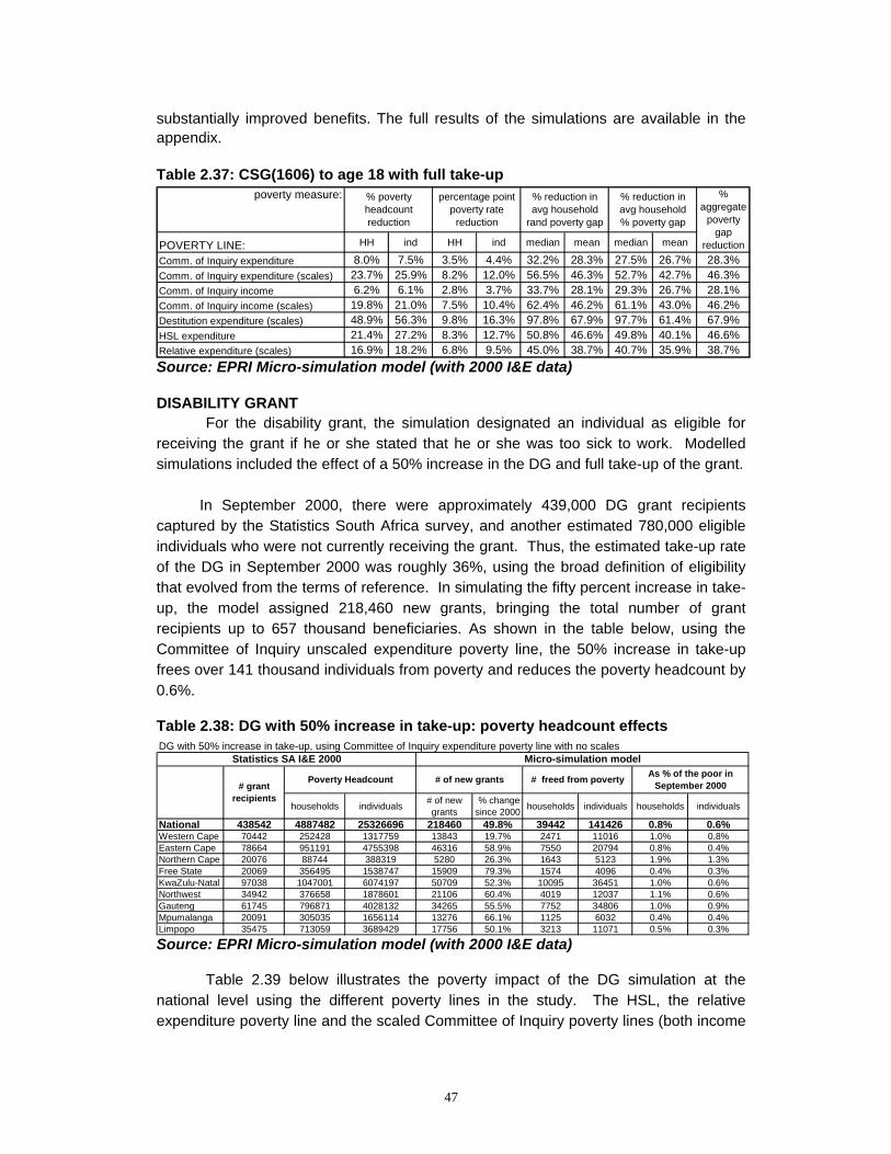
47
substantially improved benefits. The full results of the simulations are available in the appendix. Table 2.37: CSG(1606) to age 18 with full take-up
Source: EPRI Micro-simulation model (with 2000 I&E data) DISABILITY GRANT
For the disability grant, the simulation designated an individual as eligible for receiving the grant if he or she stated that he or she was too sick to work. Modelled simulations included the effect of a 50% increase in the DG and full take-up of the grant. In September 2000, there were approximately 439,000 DG grant recipients captured by the Statistics South Africa survey, and another estimated 780,000 eligible individuals who were not currently receiving the grant. Thus, the estimated take-up rate of the DG in September 2000 was roughly 36%, using the broad definition of eligibility that evolved from the terms of reference. In simulating the fifty percent increase in take-up, the model assigned 218,460 new grants, bringing the total number of grant recipients up to 657 thousand beneficiaries. As shown in the table below, using the Committee of Inquiry unscaled expenditure poverty line, the 50% increase in take-up frees over 141 thousand individuals from poverty and reduces the poverty headcount by 0.6%. Table 2.38: DG with 50% increase in take-up: poverty headcount effects
Source: EPRI Micro-simulation model (with 2000 I&E data)
Table 2.39 below illustrates the poverty impact of the DG simulation at the national level using the different poverty lines in the study. The HSL, the relative expenditure poverty line and the scaled Committee of Inquiry poverty lines (both income
poverty measure:
POVERTY LINE: HH ind HH ind median mean median mean
Comm. of Inquiry expenditure 8.0% 7.5% 3.5% 4.4% 32.2% 28.3% 27.5% 26.7% 28.3%Comm. of Inquiry expenditure (scales) 23.7% 25.9% 8.2% 12.0% 56.5% 46.3% 52.7% 42.7% 46.3%Comm. of Inquiry income 6.2% 6.1% 2.8% 3.7% 33.7% 28.1% 29.3% 26.7% 28.1%Comm. of Inquiry income (scales) 19.8% 21.0% 7.5% 10.4% 62.4% 46.2% 61.1% 43.0% 46.2%Destitution expenditure (scales) 48.9% 56.3% 9.8% 16.3% 97.8% 67.9% 97.7% 61.4% 67.9%HSL expenditure 21.4% 27.2% 8.3% 12.7% 50.8% 46.6% 49.8% 40.1% 46.6%Relative expenditure (scales) 16.9% 18.2% 6.8% 9.5% 45.0% 38.7% 40.7% 35.9% 38.7%
% aggregate
poverty gap
reduction
% poverty headcount reduction
percentage point poverty rate
reduction
% reduction in avg household
rand poverty gap
% reduction in avg household % poverty gap
DG with 50% increase in take-up, using Committee of Inquiry expenditure poverty line with no scales
households individuals # of new grants
% change since 2000 households individuals households individuals
National 438542 4887482 25326696 218460 49.8% 39442 141426 0.8% 0.6%Western Cape 70442 252428 1317759 13843 19.7% 2471 11016 1.0% 0.8%Eastern Cape 78664 951191 4755398 46316 58.9% 7550 20794 0.8% 0.4%Northern Cape 20076 88744 388319 5280 26.3% 1643 5123 1.9% 1.3%Free State 20069 356495 1538747 15909 79.3% 1574 4096 0.4% 0.3%KwaZulu-Natal 97038 1047001 6074197 50709 52.3% 10095 36451 1.0% 0.6%Northwest 34942 376658 1878601 21106 60.4% 4019 12037 1.1% 0.6%Gauteng 61745 796871 4028132 34265 55.5% 7752 34806 1.0% 0.9%Mpumalanga 20091 305035 1656114 13276 66.1% 1125 6032 0.4% 0.4%Limpopo 35475 713059 3689429 17756 50.1% 3213 11071 0.5% 0.3%
# of new grants # freed from poverty As % of the poor in September 2000
Micro-simulation modelStatistics SA I&E 2000
Poverty Headcount# grant
recipients
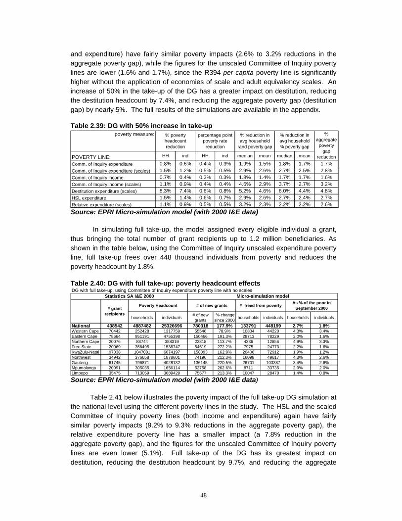
48
and expenditure) have fairly similar poverty impacts (2.6% to 3.2% reductions in the aggregate poverty gap), while the figures for the unscaled Committee of Inquiry poverty lines are lower (1.6% and 1.7%), since the R394 per capita poverty line is significantly higher without the application of economies of scale and adult equivalency scales. An increase of 50% in the take-up of the DG has a greater impact on destitution, reducing the destitution headcount by 7.4%, and reducing the aggregate poverty gap (destitution gap) by nearly 5%. The full results of the simulations are available in the appendix. Table 2.39: DG with 50% increase in take-up
Source: EPRI Micro-simulation model (with 2000 I&E data)
In simulating full take-up, the model assigned every eligible individual a grant, thus bringing the total number of grant recipients up to 1.2 million beneficiaries. As shown in the table below, using the Committee of Inquiry unscaled expenditure poverty line, full take-up frees over 448 thousand individuals from poverty and reduces the poverty headcount by 1.8%. Table 2.40: DG with full take-up: poverty headcount effects
Source: EPRI Micro-simulation model (with 2000 I&E data) Table 2.41 below illustrates the poverty impact of the full take-up DG simulation at the national level using the different poverty lines in the study. The HSL and the scaled Committee of Inquiry poverty lines (both income and expenditure) again have fairly similar poverty impacts (9.2% to 9.3% reductions in the aggregate poverty gap), the relative expenditure poverty line has a smaller impact (a 7.8% reduction in the aggregate poverty gap), and the figures for the unscaled Committee of Inquiry poverty lines are even lower (5.1%). Full take-up of the DG has its greatest impact on destitution, reducing the destitution headcount by 9.7%, and reducing the aggregate
poverty measure:
POVERTY LINE: HH ind HH ind median mean median mean
Comm. of Inquiry expenditure 0.8% 0.6% 0.4% 0.3% 1.9% 1.5% 1.8% 1.7% 1.7%Comm. of Inquiry expenditure (scales) 1.5% 1.2% 0.5% 0.5% 2.9% 2.6% 2.7% 2.5% 2.8%Comm. of Inquiry income 0.7% 0.4% 0.3% 0.3% 1.8% 1.4% 1.7% 1.7% 1.6%Comm. of Inquiry income (scales) 1.1% 0.9% 0.4% 0.4% 4.6% 2.9% 3.7% 2.7% 3.2%Destitution expenditure (scales) 8.3% 7.4% 0.6% 0.8% 5.2% 4.6% 6.0% 4.4% 4.8%HSL expenditure 1.5% 1.4% 0.6% 0.7% 2.9% 2.6% 2.7% 2.4% 2.7%Relative expenditure (scales) 1.1% 0.9% 0.5% 0.5% 3.2% 2.3% 2.2% 2.2% 2.6%
% poverty headcount reduction
percentage point poverty rate
reduction
% reduction in avg household
rand poverty gap
% reduction in avg household % poverty gap
% aggregate
poverty gap
reduction
DG with full take-up, using Committee of Inquiry expenditure poverty line with no scales
households individuals # of new grants
% change since 2000 households individuals households individuals
National 438542 4887482 25326696 780318 177.9% 133791 448199 2.7% 1.8%Western Cape 70442 252428 1317759 55546 78.9% 10804 44220 4.3% 3.4%Eastern Cape 78664 951191 4755398 150466 191.3% 28713 78229 3.0% 1.6%Northern Cape 20076 88744 388319 22818 113.7% 4336 12856 4.9% 3.3%Free State 20069 356495 1538747 54619 272.2% 7975 24773 2.2% 1.6%KwaZulu-Natal 97038 1047001 6074197 158093 162.9% 20406 72912 1.9% 1.2%Northwest 34942 376658 1878601 74196 212.3% 16098 49617 4.3% 2.6%Gauteng 61745 796871 4028132 136145 220.5% 26701 103387 3.4% 2.6%Mpumalanga 20091 305035 1656114 52758 262.6% 8711 33735 2.9% 2.0%Limpopo 35475 713059 3689429 75677 213.3% 10047 28470 1.4% 0.8%
# of new grants # freed from poverty As % of the poor in September 2000
Micro-simulation modelStatistics SA I&E 2000
Poverty Headcount# grant
recipients
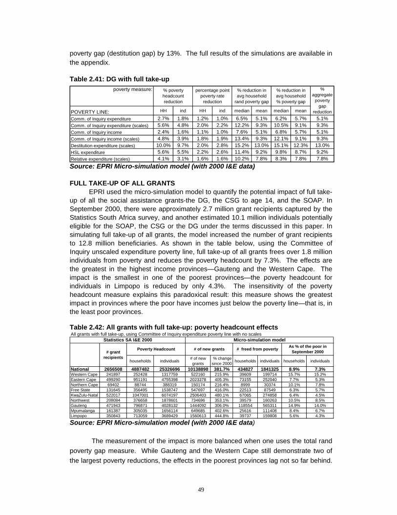
49
poverty gap (destitution gap) by 13%. The full results of the simulations are available in the appendix. Table 2.41: DG with full take-up
Source: EPRI Micro-simulation model (with 2000 I&E data) FULL TAKE-UP OF ALL GRANTS EPRI used the micro-simulation model to quantify the potential impact of full take-up of all the social assistance grants-the DG, the CSG to age 14, and the SOAP. In September 2000, there were approximately 2.7 million grant recipients captured by the Statistics South Africa survey, and another estimated 10.1 million individuals potentially eligible for the SOAP, the CSG or the DG under the terms discussed in this paper. In simulating full take-up of all grants, the model increased the number of grant recipients to 12.8 million beneficiaries. As shown in the table below, using the Committee of Inquiry unscaled expenditure poverty line, full take-up of all grants frees over 1.8 million individuals from poverty and reduces the poverty headcount by 7.3%. The effects are the greatest in the highest income provinces—Gauteng and the Western Cape. The impact is the smallest in one of the poorest provinces—the poverty headcount for individuals in Limpopo is reduced by only 4.3%. The insensitivity of the poverty headcount measure explains this paradoxical result: this measure shows the greatest impact in provinces where the poor have incomes just below the poverty line—that is, in the least poor provinces. Table 2.42: All grants with full take-up: poverty headcount effects
Source: EPRI Micro-simulation model (with 2000 I&E data)
The measurement of the impact is more balanced when one uses the total rand poverty gap measure. While Gauteng and the Western Cape still demonstrate two of the largest poverty reductions, the effects in the poorest provinces lag not so far behind.
poverty measure:
POVERTY LINE: HH ind HH ind median mean median mean
Comm. of Inquiry expenditure 2.7% 1.8% 1.2% 1.0% 6.5% 5.1% 6.2% 5.7% 5.1%Comm. of Inquiry expenditure (scales) 5.6% 4.8% 2.0% 2.2% 12.2% 9.3% 10.5% 9.1% 9.3%Comm. of Inquiry income 2.4% 1.6% 1.1% 1.0% 7.6% 5.1% 6.8% 5.7% 5.1%Comm. of Inquiry income (scales) 4.8% 3.9% 1.8% 1.9% 13.4% 9.3% 12.1% 9.1% 9.3%Destitution expenditure (scales) 10.0% 9.7% 2.0% 2.8% 15.2% 13.0% 15.1% 12.3% 13.0%HSL expenditure 5.6% 5.5% 2.2% 2.6% 11.4% 9.2% 9.8% 8.7% 9.2%Relative expenditure (scales) 4.1% 3.1% 1.6% 1.6% 10.2% 7.8% 8.3% 7.8% 7.8%
% aggregate
poverty gap
reduction
% poverty headcount reduction
percentage point poverty rate
reduction
% reduction in avg household
rand poverty gap
% reduction in avg household % poverty gap
All grants with full take-up, using Committee of Inquiry expenditure poverty line with no scales
households individuals # of new grants
% change since 2000 households individuals households individuals
National 2656508 4887482 25326696 10138898 381.7% 434827 1841325 8.9% 7.3%Western Cape 241897 252428 1317759 522160 215.9% 39609 199714 15.7% 15.2%Eastern Cape 499290 951191 4755398 2023378 405.3% 73155 252040 7.7% 5.3%Northern Cape 69402 88744 388319 150174 216.4% 8999 30374 10.1% 7.8%Free State 131645 356495 1538747 547697 416.0% 22513 87549 6.3% 5.7%KwaZulu-Natal 522017 1047001 6074197 2506403 480.1% 67065 274858 6.4% 4.5%Northwest 208084 376658 1878601 734696 353.1% 39579 160263 10.5% 8.5%Gauteng 471943 796871 4028132 1444092 306.0% 118554 565311 14.9% 14.0%Mpumalanga 161387 305035 1656114 649685 402.6% 25616 111408 8.4% 6.7%Limpopo 350843 713059 3689429 1560613 444.8% 39737 159808 5.6% 4.3%
# of new grants # freed from poverty As % of the poor in September 2000
Micro-simulation modelStatistics SA I&E 2000
Poverty Headcount# grant
recipients
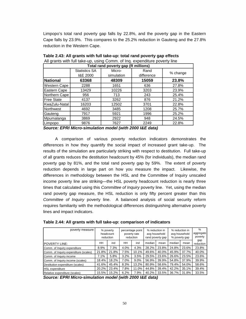
50
Limpopo’s total rand poverty gap falls by 22.8%, and the poverty gap in the Eastern Cape falls by 23.9%. This compares to the 25.2% reduction in Gauteng and the 27.8% reduction in the Western Cape. Table 2.43: All grants with full take-up: total rand poverty gap effects
Source: EPRI Micro-simulation model (with 2000 I&E data) A comparison of various poverty reduction indicators demonstrates the differences in how they quantify the social impact of increased grant take-up. The results of the simulation are particularly striking with respect to destitution. Full take-up of all grants reduces the destitution headcount by 45% (for individuals), the median rand poverty gap by 81%, and the total rand poverty gap by 59%. The extent of poverty reduction depends in large part on how you measure the impact. Likewise, the differences in methodology between the HSL and the Committee of Inquiry unscaled income poverty line are striking—the HSL poverty headcount reduction is nearly three times that calculated using this Committee of Inquiry poverty line. Yet, using the median rand poverty gap measure, the HSL reduction is only fifty percent greater than this Committee of Inquiry poverty line. A balanced analysis of social security reform requires familiarity with the methodological differences distinguishing alternative poverty lines and impact indicators. Table 2.44: All grants with full take-up: comparison of indicators
Source: EPRI Micro-simulation model (with 2000 I&E data)
poverty measure:
POVERTY LINE: HH ind HH ind median mean median mean
Comm. of Inquiry expenditure 8.9% 7.3% 4.0% 4.3% 28.2% 23.8% 24.8% 23.6% 23.8%Comm. of Inquiry expenditure (scales) 21.8% 21.8% 7.5% 10.1% 49.6% 40.0% 45.9% 37.7% 40.0%Comm. of Inquiry income 7.1% 5.8% 3.2% 3.5% 29.5% 23.6% 26.6% 23.5% 23.6%Comm. of Inquiry income (scales) 18.4% 18.2% 7.0% 9.0% 56.9% 39.9% 54.8% 37.9% 39.9%Destitution expenditure (scales) 41.6% 45.4% 8.3% 13.2% 80.9% 58.6% 79.4% 54.0% 58.6%HSL expenditure 20.2% 23.4% 7.8% 11.0% 44.8% 39.4% 42.2% 35.1% 39.4%Relative expenditure (scales) 15.5% 15.2% 6.2% 7.9% 40.2% 33.5% 36.7% 31.8% 33.5%
% poverty headcount reduction
percentage point poverty rate
reduction
% reduction in avg household
rand poverty gap
% reduction in avg household % poverty gap
% aggregate
poverty gap
reduction
All grants with full take-up, using Comm. of Inq. expenditure poverty line
Statistics SA I&E 2000
Micro- simulation
Rand difference % change
National 63368 48309 15059 23.8%Western Cape 2288 1651 636 27.8%Eastern Cape 13429 10226 3203 23.9%Northern Cape 956 713 243 25.4%Free State 4137 3262 876 21.2%KwaZulu-Natal 16203 12502 3701 22.8%Northwest 4692 3485 1208 25.7%Gauteng 7917 5921 1996 25.2%Mpumalanga 3869 2922 948 24.5%Limpopo 9876 7627 2249 22.8%
Total rand poverty gap (R millions)
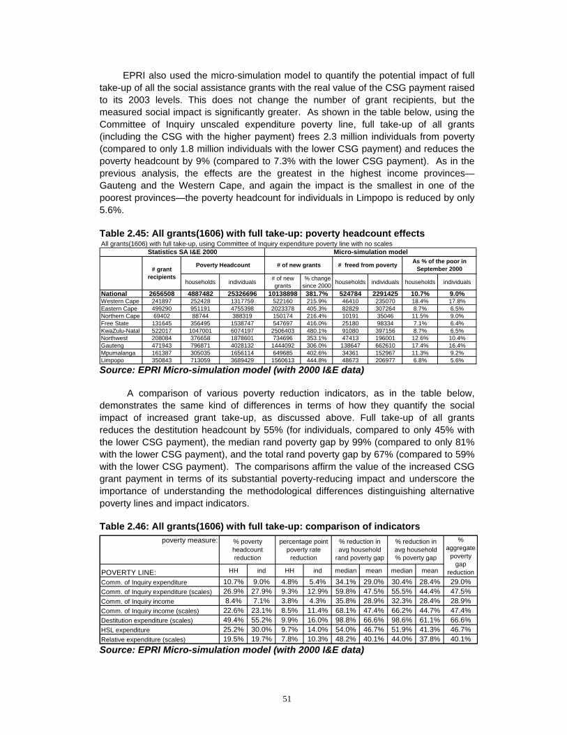
51
EPRI also used the micro-simulation model to quantify the potential impact of full take-up of all the social assistance grants with the real value of the CSG payment raised to its 2003 levels. This does not change the number of grant recipients, but the measured social impact is significantly greater. As shown in the table below, using the Committee of Inquiry unscaled expenditure poverty line, full take-up of all grants (including the CSG with the higher payment) frees 2.3 million individuals from poverty (compared to only 1.8 million individuals with the lower CSG payment) and reduces the poverty headcount by 9% (compared to 7.3% with the lower CSG payment). As in the previous analysis, the effects are the greatest in the highest income provinces—Gauteng and the Western Cape, and again the impact is the smallest in one of the poorest provinces—the poverty headcount for individuals in Limpopo is reduced by only 5.6%. Table 2.45: All grants(1606) with full take-up: poverty headcount effects
Source: EPRI Micro-simulation model (with 2000 I&E data) A comparison of various poverty reduction indicators, as in the table below, demonstrates the same kind of differences in terms of how they quantify the social impact of increased grant take-up, as discussed above. Full take-up of all grants reduces the destitution headcount by 55% (for individuals, compared to only 45% with the lower CSG payment), the median rand poverty gap by 99% (compared to only 81% with the lower CSG payment), and the total rand poverty gap by 67% (compared to 59% with the lower CSG payment). The comparisons affirm the value of the increased CSG grant payment in terms of its substantial poverty-reducing impact and underscore the importance of understanding the methodological differences distinguishing alternative poverty lines and impact indicators. Table 2.46: All grants(1606) with full take-up: comparison of indicators
Source: EPRI Micro-simulation model (with 2000 I&E data)
poverty measure:
POVERTY LINE: HH ind HH ind median mean median mean
Comm. of Inquiry expenditure 10.7% 9.0% 4.8% 5.4% 34.1% 29.0% 30.4% 28.4% 29.0%Comm. of Inquiry expenditure (scales) 26.9% 27.9% 9.3% 12.9% 59.8% 47.5% 55.5% 44.4% 47.5%Comm. of Inquiry income 8.4% 7.1% 3.8% 4.3% 35.8% 28.9% 32.3% 28.4% 28.9%Comm. of Inquiry income (scales) 22.6% 23.1% 8.5% 11.4% 68.1% 47.4% 66.2% 44.7% 47.4%Destitution expenditure (scales) 49.4% 55.2% 9.9% 16.0% 98.8% 66.6% 98.6% 61.1% 66.6%HSL expenditure 25.2% 30.0% 9.7% 14.0% 54.0% 46.7% 51.9% 41.3% 46.7%Relative expenditure (scales) 19.5% 19.7% 7.8% 10.3% 48.2% 40.1% 44.0% 37.8% 40.1%
% aggregate
poverty gap
reduction
% poverty headcount reduction
percentage point poverty rate
reduction
% reduction in avg household
rand poverty gap
% reduction in avg household % poverty gap
All grants(1606) with full take-up, using Committee of Inquiry expenditure poverty line with no scales
households individuals # of new grants
% change since 2000 households individuals households individuals
National 2656508 4887482 25326696 10138898 381.7% 524784 2291425 10.7% 9.0%Western Cape 241897 252428 1317759 522160 215.9% 46410 235070 18.4% 17.8%Eastern Cape 499290 951191 4755398 2023378 405.3% 82829 307264 8.7% 6.5%Northern Cape 69402 88744 388319 150174 216.4% 10191 35046 11.5% 9.0%Free State 131645 356495 1538747 547697 416.0% 25180 98334 7.1% 6.4%KwaZulu-Natal 522017 1047001 6074197 2506403 480.1% 91080 397156 8.7% 6.5%Northwest 208084 376658 1878601 734696 353.1% 47413 196001 12.6% 10.4%Gauteng 471943 796871 4028132 1444092 306.0% 138647 662610 17.4% 16.4%Mpumalanga 161387 305035 1656114 649685 402.6% 34361 152967 11.3% 9.2%Limpopo 350843 713059 3689429 1560613 444.8% 48673 206977 6.8% 5.6%
# of new grants # freed from poverty As % of the poor in September 2000
Micro-simulation modelStatistics SA I&E 2000
Poverty Headcount# grant
recipients
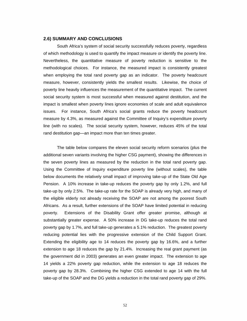
52
2.6) SUMMARY AND CONCLUSIONS South Africa’s system of social security successfully reduces poverty, regardless
of which methodology is used to quantify the impact measure or identify the poverty line.
Nevertheless, the quantitative measure of poverty reduction is sensitive to the
methodological choices. For instance, the measured impact is consistently greatest
when employing the total rand poverty gap as an indicator. The poverty headcount
measure, however, consistently yields the smallest results. Likewise, the choice of
poverty line heavily influences the measurement of the quantitative impact. The current
social security system is most successful when measured against destitution, and the
impact is smallest when poverty lines ignore economies of scale and adult equivalence
issues. For instance, South Africa’s social grants reduce the poverty headcount
measure by 4.3%, as measured against the Committee of Inquiry’s expenditure poverty
line (with no scales). The social security system, however, reduces 45% of the total
rand destitution gap—an impact more than ten times greater.
The table below compares the eleven social security reform scenarios (plus the
additional seven variants involving the higher CSG payment), showing the differences in
the seven poverty lines as measured by the reduction in the total rand poverty gap.
Using the Committee of Inquiry expenditure poverty line (without scales), the table
below documents the relatively small impact of improving take-up of the State Old Age
Pension. A 10% increase in take-up reduces the poverty gap by only 1.2%, and full
take-up by only 2.5%. The take-up rate for the SOAP is already very high, and many of
the eligible elderly not already receiving the SOAP are not among the poorest South
Africans. As a result, further extensions of the SOAP have limited potential in reducing
poverty. Extensions of the Disability Grant offer greater promise, although at
substantially greater expense. A 50% increase in DG take-up reduces the total rand
poverty gap by 1.7%, and full take-up generates a 5.1% reduction. The greatest poverty
reducing potential lies with the progressive extension of the Child Support Grant.
Extending the eligibility age to 14 reduces the poverty gap by 16.6%, and a further
extension to age 18 reduces the gap by 21.4%. Increasing the real grant payment (as
the government did in 2003) generates an even greater impact. The extension to age
14 yields a 22% poverty gap reduction, while the extension to age 18 reduces the
poverty gap by 28.3%. Combining the higher CSG extended to age 14 with the full
take-up of the SOAP and the DG yields a reduction in the total rand poverty gap of 29%.
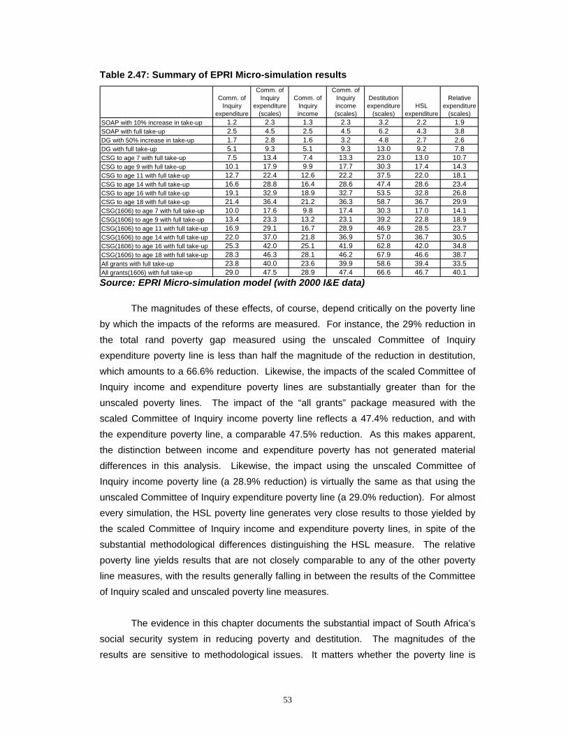
53
Table 2.47: Summary of EPRI Micro-simulation results
Source: EPRI Micro-simulation model (with 2000 I&E data)
The magnitudes of these effects, of course, depend critically on the poverty line by which the impacts of the reforms are measured. For instance, the 29% reduction in the total rand poverty gap measured using the unscaled Committee of Inquiry expenditure poverty line is less than half the magnitude of the reduction in destitution, which amounts to a 66.6% reduction. Likewise, the impacts of the scaled Committee of Inquiry income and expenditure poverty lines are substantially greater than for the unscaled poverty lines. The impact of the “all grants” package measured with the scaled Committee of Inquiry income poverty line reflects a 47.4% reduction, and with the expenditure poverty line, a comparable 47.5% reduction. As this makes apparent, the distinction between income and expenditure poverty has not generated material differences in this analysis. Likewise, the impact using the unscaled Committee of Inquiry income poverty line (a 28.9% reduction) is virtually the same as that using the unscaled Committee of Inquiry expenditure poverty line (a 29.0% reduction). For almost every simulation, the HSL poverty line generates very close results to those yielded by the scaled Committee of Inquiry income and expenditure poverty lines, in spite of the substantial methodological differences distinguishing the HSL measure. The relative poverty line yields results that are not closely comparable to any of the other poverty line measures, with the results generally falling in between the results of the Committee of Inquiry scaled and unscaled poverty line measures.
The evidence in this chapter documents the substantial impact of South Africa’s social security system in reducing poverty and destitution. The magnitudes of the results are sensitive to methodological issues. It matters whether the poverty line is
Comm. of Inquiry
expenditure
Comm. of Inquiry
expenditure (scales)
Comm. of Inquiry income
Comm. of Inquiry income (scales)
Destitution expenditure
(scales) HSL
expenditure
Relative expenditure
(scales) SOAP with 10% increase in take-up 1.2 2.3 1.3 2.3 3.2 2.2 1.9SOAP with full take-up 2.5 4.5 2.5 4.5 6.2 4.3 3.8DG with 50% increase in take-up 1.7 2.8 1.6 3.2 4.8 2.7 2.6DG with full take-up 5.1 9.3 5.1 9.3 13.0 9.2 7.8CSG to age 7 with full take-up 7.5 13.4 7.4 13.3 23.0 13.0 10.7CSG to age 9 with full take-up 10.1 17.9 9.9 17.7 30.3 17.4 14.3CSG to age 11 with full take-up 12.7 22.4 12.6 22.2 37.5 22.0 18.1CSG to age 14 with full take-up 16.6 28.8 16.4 28.6 47.4 28.6 23.4CSG to age 16 with full take-up 19.1 32.9 18.9 32.7 53.5 32.8 26.8CSG to age 18 with full take-up 21.4 36.4 21.2 36.3 58.7 36.7 29.9CSG(1606) to age 7 with full take-up 10.0 17.6 9.8 17.4 30.3 17.0 14.1CSG(1606) to age 9 with full take-up 13.4 23.3 13.2 23.1 39.2 22.8 18.9CSG(1606) to age 11 with full take-up 16.9 29.1 16.7 28.9 46.9 28.5 23.7CSG(1606) to age 14 with full take-up 22.0 37.0 21.8 36.9 57.0 36.7 30.5CSG(1606) to age 16 with full take-up 25.3 42.0 25.1 41.9 62.8 42.0 34.8CSG(1606) to age 18 with full take-up 28.3 46.3 28.1 46.2 67.9 46.6 38.7All grants with full take-up 23.8 40.0 23.6 39.9 58.6 39.4 33.5All grants(1606) with full take-up 29.0 47.5 28.9 47.4 66.6 46.7 40.1
54
relative or absolute, whether it is scaled for household composition and economies of scale or not, and to a small extent whether it measures income or expenditure. Likewise, it matters how the poverty impact is measured—using poverty headcount or variants on the poverty gap. Nevertheless, the qualitative results, and the answers to critical policy questions, are robust to different methodological approaches. South Africa’s system of social security substantially reduces deprivation, and the progressive extension of the magnitude, scope and reach of social grants holds the potential to dramatically diminish the prevalence of poverty in South Africa.
55
CHAPTER 3)
The Household Impact of Social Assistance Programmes
3.1) INTRODUCTION This chapter evaluates the impact of South Africa’s social development grants
on the well being of individuals and households, evaluating how social security affects household behaviour and access to basic needs, including education, health care, nutrition and other requirements. The previous chapter focused on aggregate household income and expenditure—some of the most common variables used in the measurement of poverty. This chapter broadens the focus, examining dis-aggregated as well as non-monetary measures of well being. The chapter focuses on the main social grants, with a particular emphasis on the State Old Age Pension (SOAP), the Child Support Grant (CSG) and the Disability Grant (DG). Targeted social programmes that provide cash transfers to the poor often have consequences for the behaviour of untargeted individuals due to income sharing within households. Because of income pooling within households, these grants have broad household impacts. This study quantifies these effects, using a linked data set of Statistic South Africa’s Income and Expenditure Survey (IES) in October 2000 and Labour Force Survey (LFS) in September 2000, as well as previous October Household Surveys.
3.2) BACKGROUND AND LITERATURE REVIEW
Non-contributory pension programmes have been adopted in several countries in Latin America and Africa, including Brazil, Argentina, Namibia, Botswana, and South Africa. In a study that reviews research on the pension programmes in these countries, Barrientos and Lloyd-Sherlock10 report the overall positive impacts on poverty. Extreme poverty is 16% lower in households with pension income than in those without pension income in Argentina. Headcount poverty among households with pensioners is significantly lower than those without in Brazil. In Namibia, access to a pension is associated with out-migration from rural areas, suggesting that young adults migrate to cities to look for jobs. Consistent with the finding in South Africa that pensions provided to women have greater impacts on the welfare of the household, one study in Brazil reports that there is a strong association between the presence of female pensioners and school enrolment of girls aged between 12 and 14. These international studies indicate that non-contributory pension programmes in developing countries play important roles in improving social welfare of the poor households.
The effectiveness of South Africa’s SOAP in reaching poor households and improving their welfare has also been widely recognised. The non-contributory pension programme was initially intended to provide a social safety net for the aged poor, who were vulnerable in the household because of “a decline in job opportunities, increased vulnerability to health conditions, limited mobility, discrimination in access to credit and
10 Barrientos, and Lloyd-Sherlock (2002).
56
financial markets, and changes in household composition and status” (Barrientos and Lloyd-Sherlock, 5). However, the benefits of the pension are found to be distributed more broadly to all members in the household because the majority of the poor households in South Africa live in multi-generation households.
Economic research usually measures the welfare of the household using income levels, expenditure patterns, health conditions, and education access. However, there exists considerable debate about how to most accurately measure the true well being of a household or an individual. Case and Deaton11 address the question of appropriate poverty measures for individual members in the household. They are specifically concerned with the differences in male and female individuals within the household, as standard income poverty measures regard all members of the household under a specified income level as "poor." They conclude that health and education are better measures of individual welfare (or poverty) than income and expenditures, because the survey questions in these two categories are usually targeted to individuals rather than to household heads.
Precise and useful measures of education and health, however, are difficult to obtain. For example, while subjective measures, such as years of education and literacy, can quantify some dimensions of education, there is no easily quantified measure of school quality in South Africa. Appropriate measures for health are also difficult to identify. One important methodology for children's health and nutrition employs anthropometric indicators, such as height-for-age and weight-for-height. Using the child anthropometric indicators, Duflo finds that the household with an eligible woman for SOAP increases the weight-for-height of girls significantly, while there was no effect on boys and in the household with an eligible man (Duflo, 2000). Her findings are relevant to the present study: household characteristics are similar between the household with an eligible man and with an eligible woman. This supports the comparison of the impact of the presence of female and male pensioners in the household, given Duflo’s evidence suggesting that there are no significant unobservable differences in household characteristics between the two groups. She also points out that the unobserved correlation between SOAP and other public transfers, such as the CSG, may overestimate the impact of SOAP. In order to isolate the impact of the SOAP, it is important to control for other social development grants that households are receiving. In the data sets from 2000 employed by this present study, however, the take up rates for other social grants are very low. As a result, this chapter evaluates household impacts controlling for the CSG and the DG (received by 2.9% and 3.4% of all households respectively), because the other grants are received by less than 1% of the sample.
11 Case and Deaton (2002).
57
Psacharopoulos (1994) concludes that primary schooling remains ‘the number one investment priority’ for developing countries, with the social rate of return to investment in primary education averaging 24 percent in Sub-Saharan Africa and roughly 20 percent in Asia and Latin America.”12 For many poor children in South Africa, the prospects of education are severely hampered by conditions of poverty. Many poor households cannot afford to invest their limited income into education. In South Africa, “although the current constitution of the Republic of South Africa (adopted in 1996) guarantees education as a right, it is not free. In addition to the direct cost of school fees (tuition), students and their families must cover the indirect costs of books and supplies, school uniforms, and often transportation to school as well. Poorer families who are disproportionately represented among [blacks] (Klasen 1997), are less able to afford the costs of education.”13 The amount that a school may charge for tuition can vary immensely. The fee may be “as little as 50 rand to 6,000 rand and above, depending in part on the quality of the school.”14
There exists a relationship between education and poverty. “Poverty, pervasive
across the region [of Africa], is a barrier to expanding education access and improving learning outcomes.”15 “Of the 35 countries the United Nations Development Programme (UNDP) classifies as having low human development, 28 are in Sub-Saharan African (UNDP 1999). More than 40 percent of Africans live below the $1 a day poverty line, and the incidence of poverty as well as the absolute numbers of people living in poverty have increased since the late 1980s.”16 Investments in education by governments and households are hindered by the vast amounts of poverty, resulting in low educational attainment.17
“When households become impoverished, older children are often pulled out of school to supplement family income and pay for the school fees of younger siblings.”18 Overall enrolment rates are drastically lower for the poor at all levels. This is particularly true at the secondary level.19 In addition, even if those who are poor remain in school, these children often spend more time contributing to the household income than those children from better off households. “As a result they are less likely to spend out-of-school hours on schoolwork, more likely to be absent from school during periods of peak labour demand, and more likely to be tired and ill-prepared for learning when they are in the classroom.”20
12 Case (2001). 13 Anderson (2001). 14 Anderson (2001). 15 World Bank (2001). 16 World Bank (2001). 17 World Bank (2001). 18 UNICEF (2001). 19 Catro et al. (1999). 20 World Bank (2001).
58
While poverty reduces the ability of children to attend school, education increases the ability of people to move out of poverty. “Poverty is a key obstacle to expanding access to education and improving learning outcomes in Africa, while education is instrumental in eliminating poverty.”21 It is instrumental in reducing poverty because “education develops intellectual capacity and social skills, and children who complete at least four years of schooling- considered the minimum for achieving basic literacy and numeracy- are better equipped to move out of poverty. For example, levels of education correlate with income levels and with the ability to hold a job in the formal sector.” 22
Those children that do not attend school are almost always poor, from disadvantaged groups, and are often in remote areas. “Nearly 60 percent of out-of-school children in Africa are girls.”23 Educating children, particularly girls is key to combating poverty. “Educated girls have greater confidence to make decisions for themselves. They marry later in life and are more likely to space out their pregnancies. As a result, they tend to have fewer children and are more likely to seek medical attention for themselves and their children. They are better informed about good nutrition and childcare. Women who were educated as girls are far more likely to enrol their own children in primary school. Educating children, particularly girls, is therefore a critical part of breaking the inter-generational cycle of poverty.”24 In South Africa, the fraction of children living with a pensioner is highest among children whose household per capita incomes are the lowest, so that the pension not only reaches the households in which the children live, but disproportionately reaches children in poverty.”25 The money reaching impoverished children augments the pool that pays for their school fees.
Case studies the impacts of SOAP on health status, comparing households where income is pooled with those where income is not pooled (Case, 2001). She uses height-for-weight and self-reported health conditions as measures of health for children and adults respectively. Although self-reporting is often considered an inconsistent measure, Case and Deaton (2002) show that it is genuinely useful. Their result was intuitive: health status in the household with income pooling improves for all members while health status in the household without income pooling improves the most for the pensioners.
On the subject of expenditure patterns, there are two opposing studies on the impacts of SOAP, which are useful to review for this study. The study by Case and
21 World Bank (2001). 22 UNICEF (2001). 23 World Bank (2001). 24 UNICEF(2001). 25 Case and Deaton (1996).

59
Deaton (1998)26 reports that the SOAP is well targeted to the poorest households and households with children. Their results show that the expenditure share of pension income on food is not significantly different from that of non-pension income. This finding supports the hypothesis of income pooling, represented in their words as the idea of “a rand is a rand.” More recently, Maitra and Ray (2003) find social grant impacts on expenditure patterns that contradict Case and Deaton’s earlier findings that the expenditure allocation of pension income is strikingly similar to that of other income. While Maitra and Ray emphasise the importance of public and private transfers in reducing poverty, they also find that poor households have a fundamentally different expenditure pattern compared to non-poor households, and that expenditure patterns significantly differ with the source of income.
Maitra and Ray’s finding of the endogeneity of income flows27 (regular income, pension income and private transfers) raises an important question for this study. They analyse the relationship between different income and expenditure shares. Their results show that the households that receive private transfers and those that receive public pensions both have higher expenditure shares on food and education, and lower expenditure shares on alcohol, tobacco and entertainment than other households do. This suggests that an increase in pension income or other social grants may have opposite effects on certain expenditure shares, compared to an increase in earned income. An increase in regular income generally decreases the expenditure share on food and increases the share spent on entertainment. They explain these different patterns of expenditures as evidence of non-income pooling: who receives the transfer within the household matters. In the case of the SOAP, it is likely that elderly pensioners allocate the resources differently compared to the household heads that are often of working age. They also find that the amount of pension is positively correlated with the number of the eligible members and negatively correlated with the number of children and adults. These findings inform this present study, which constructs a model to control for the endogeneity of income in order to evaluate the impacts of pension amounts as well as the influence of the demographic composition of the household.
The literature surveyed documents the importance of using a variety of welfare measures to evaluate the impacts of social grants. The present study employs the household school attendance rate as an education measure, the access to piped water and expenditure shares on medical care for non-aid members as health measures, and expenditure shares on food and the prevalence of adult and child hunger as measures of nutrition.
26 Case and Deaton (1998). 27 Endogeneity of income flows refers to Maitra and Ray’s finding that the amount of income from one source is one of the determinants of the other types of incomes.
60
Empirical studies demonstrate the powerful impact of the SOAP as an instrument of poverty reduction. However, most of the studies have been conducted with data collected in 1995 or earlier. As the take-up rates for social grants have increased dramatically in the past several years, more current data has the potential to illuminate a better understanding of the household impact of social development. This present study employs the Income and Expenditure Survey from 2000 and the Labour Force Surveys from 2000, 2001 and 2002, all conducted by Statistics South Africa. This is the most current nationally representative survey data available at the time of the study. 3.3) SOCIAL SECURITY AND EDUCATION
Economic theory suggests that social grants, by raising incomes, affect education in three ways. First, to the extent that there are financial barriers to school attendance – purchasing school supplies, uniforms, tuition, transportation, etc. – the boost in disposable income provided by a social grant could help pay the otherwise unaffordable costs of attending school. Second, a grant could relieve the opportunity cost of school attendance; with a cash transfer in hand, a family might be more able to forgo a child’s contribution to household income (or food production in the case of subsistence farmers) in favour of making a long-term investment in education. Third, by indirectly increasing the resources available to schools, the quality of education may improve, making education a more attractive option to households. This chapter quantifies these effects using econometric models that evaluate the correlation between measures of social grants and school attendance. METHODOLOGY
The education analysis in this study employs two methodologies—one that develops a three-stage model to control for the simultaneous interactions between social grants and income, and the second that explicitly controls for missing data through strong restrictions on the sample. The first methodology Statistics South Africa’s Income and Expenditure Survey from October 2000 and the Labour Force Surveys from September 2000. The second methodology uses previous October Household Surveys by Statistics South Africa.
The first methodology is based on a household expenditure model similar to that
of Maitra and Ray’s28 study of expenditure shares. In their study, Maitra and Ray use predicted income, pension income, and private transfers to isolate the effects of three income flows. As their findings show that sources of income affect expenditure patterns of the household, this present study categorises income into household pension income, household remittances, and other household income per capita to isolate the impacts of the social grants. Although the use of household total income and household income per capita produce significantly similar results, this present study uses household income per capita instead of household total income, as the number of people in the household varies from 1 to 25 in the sample. Given this variance, household income 28 Maitra and Ray (2003).
61
per capita reflects well being of the household members better than the total household income.
The model is a three-stage process. First, the model predicts household income per capita, based on actual income and other variables that quantify household characteristics. The specifications for the income prediction follow closely to those of Maitra and Ray’s29. Because income is not necessarily a linear function, the model employs linear non-linear estimation techniques, including log and quadratic specifications. In the second stage, the model predicts the pension amount, using the predicted income per capita and other household characteristics. This second stage addresses the issue of the simultaneity of income and pension, as explained by education as well as health, and nutrition variables. For instance, the education and health status of the household may determine both the household income and pension, while income and pensions in turn determine education and health status. By using income and pension variables predicted by other household characteristics, this model corrects for the possible simultaneity and resulting measurement errors.
In the third stage, the impacts of the social grants on household welfare are measured, using predicted income per capita, predicted pension amount, remittances, as well as other variables that are important determinants of household welfare. The main education measure—the school attendance rate—is calculated by taking the ratio of the number of children currently enrolled in school to the number of children between seven and sixteen years of age in the household.
There are several concerns with the data. The empirical analysis is based on the merged data set of the IES and LFS, resulting in mismatching issues. For example, some households reported receiving the SOAP in the LFS nevertheless report zero income in this category in the IES. The counts of these mismatches for some variables are as high as 10% of the sample. To evaluate the impact of the possible measurement errors on the robustness of the results, the model tested alternative hierarchies for resolving data inconsistencies and found no significant impacts on the results.
In order to control for missing data, the second part of this section uses a
methodology adopted by Bertrand, Miller and Mullainathan (2000) and focuses on the enrolment of children aged 6 to 18 living in three-generational households.30 31 By focusing on school age children living in households with both parents and grandparents, the study addresses the possibility that children who live with parents and grandparents in a single household differ systematically from their peers who live only with grandparents with respect to school attendance. Focusing on three-generational households thus reduces heterogeneity in the test sample, essentially controlling for 29 See Appendix for regression results for income and pension amount. 30 Three-generational households contain children, working age adults, and adults in pensionable age. 31 South African children begin the 1st grade at age 7 and receive their matric at the age of 17. This study expands the age range to account for the usual group of early- or late-starters present in every school system.
62
missing data—measures of this unobserved heterogeneity. In line with the methodology of Bertrand, Miller and Mullainathan (2000), the results reported in this section are further restricted to those households classified as African by Statistics South Africa.
Three-generational households are quite common in South Africa. Approximately a quarter of the households in the country contain three generations, and a large proportion of these three-generational households receiving some pension disbursement. These characteristics are consistent with findings by Case and Deaton in their analysis of the 1994 Southern Africa Labour and Development Research Unit (SALDRU) survey.
The dependent variables in the direct models are binary variables indicating full-time attendance at a school, college, technikon (technical school), or university. Three variables assess the impact of social grant transfers, that is, a level measure of monthly grant receipts, a discrete variable equal to one if households receive some pension transfer, and another discrete variable equal to one if any member of the household is eligible to receive a pension. As Bertrand et al. (2000) note, using discrete variables for household eligibility can help to account for potential endogeneity in take-up rates, the possibility that factors in the model (like the education of the household head) are determinants of pension take-up.
A key aspect of the analysis is the significance of poverty in the relationship between school enrolment and social grants. There is little reason to expect that the impact of pensions will be the same for upper income households as for lower income households; because it represents a greater relative increase in disposable income, an additional rand of social grant benefits is expected to have a stronger influence on the behaviour of lower income households. To investigate these effects the model is applied to consumption quartile sub-samples of the population as determined by per capita household expenditure. Another important aspect is the testing of differential gender effects of pension transfers on schooling. An interaction term in the specification provides insight into this question. EDUCATION ANALYSIS USING THE INCOME & EXPENDITURE SURVEY 2000 AND THE LABOUR FORCE SURVEY SEP. 2000 (EXPENDITURE MODEL) The first model uses the three-stage analysis of income along with other household variables to evaluate the impact of social grants on school attendance. Table 2 summarises the impacts of social grants on the school attendance rate. Using the Ordinary Least Squares (OLS) model, both the State Old Age Pension and the Child Support Grant are positively and significantly related to school attendance rates. The Three-Stage Least Squares (3SLS) model controls for the simultaneity, and yields virtually the same results. The second specification of the 3SLS separates the effect of the gender of the SOAP recipient. The number of female pensioners and the presence of a female household head are both associated with significantly higher school attendance rates. Control variables included in the regression models indicate effects
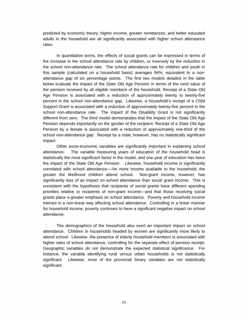
63
predicted by economic theory: higher income, greater remittances, and better educated adults in the household are all significantly associated with higher school attendance rates. In quantitative terms, the effects of social grants can be expressed in terms of the increase in the school attendance rate by children, or inversely by the reduction in the school non-attendance rate. The school attendance rate for children and youth in this sample (calculated on a household basis) averages 94%, equivalent to a non-attendance gap of six percentage points. The first two models detailed in the table below evaluate the impact of the State Old Age Pension in terms of the rand value of the pension received by all eligible members of the household. Receipt of a State Old Age Pension is associated with a reduction of approximately twenty to twenty-five percent in the school non-attendance gap. Likewise, a household’s receipt of a Child Support Grant is associated with a reduction of approximately twenty-five percent in the school non-attendance rate. The impact of the Disability Grant is not significantly different from zero. The third model demonstrates that the impact of the State Old Age Pension depends importantly on the gender of the recipient. Receipt of a State Old Age Pension by a female is associated with a reduction of approximately one-third of the school non-attendance gap. Receipt by a male, however, has no statistically significant impact. Other socio-economic variables are significantly important in explaining school attendance. The variable measuring years of education of the household head is statistically the most significant factor in the model, and one year of education has twice the impact of the State Old Age Pension. Likewise, household income is significantly correlated with school attendance-—he more income available to the household, the greater the likelihood children attend school. Non-grant income, however, has significantly less of an impact on school attendance than social grant income. This is consistent with the hypothesis that recipients of social grants have different spending priorities relative to recipients of non-grant income—and that those receiving social grants place a greater emphasis on school attendance. Poverty and household income interact in a non-linear way affecting school attendance. Controlling in a linear manner for household income, poverty continues to have a significant negative impact on school attendance. The demographics of the household also exert an important impact on school attendance. Children in households headed by women are significantly more likely to attend school. Likewise, the presence of elderly household members is associated with higher rates of school attendance, controlling for the separate effect of pension receipt. Geographic variables do not demonstrate the expected statistical significance. For instance, the variable identifying rural versus urban households is not statistically significant. Likewise, most of the provincial binary variables are not statistically significant.
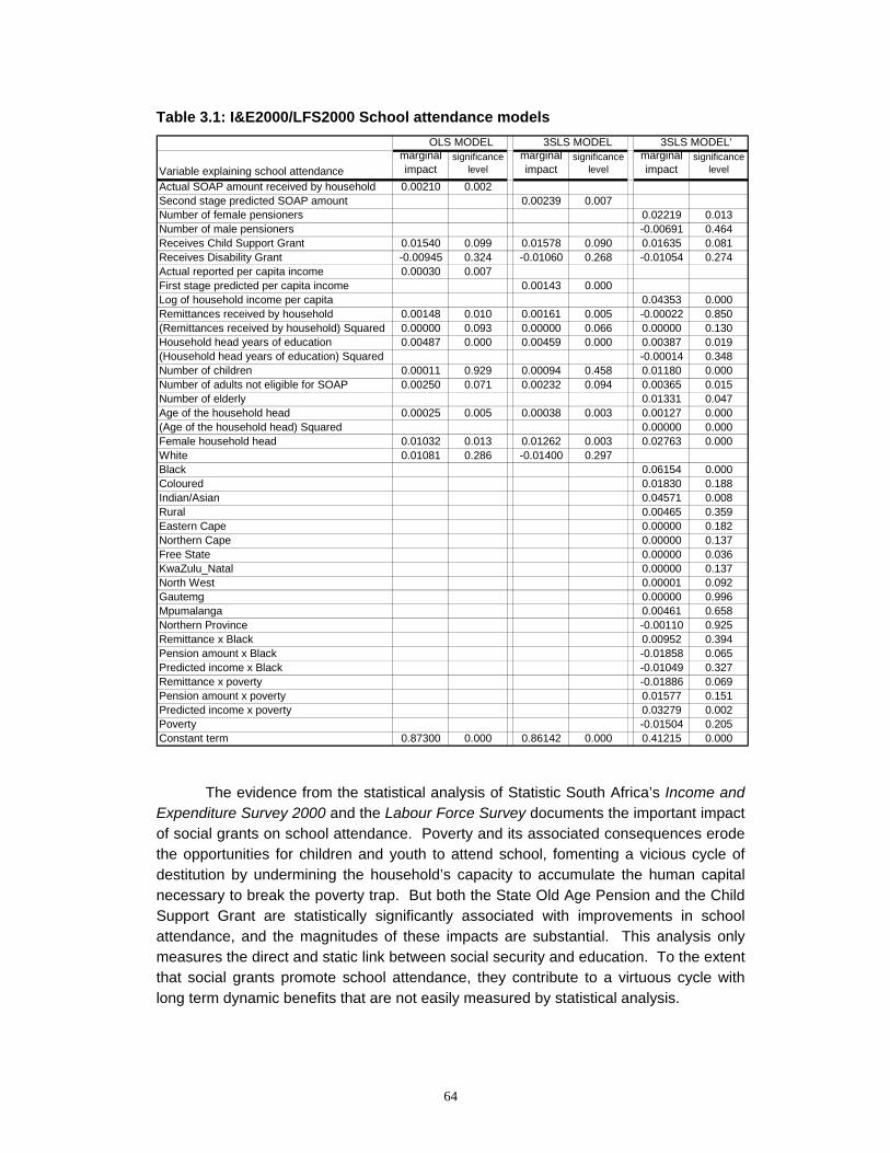
64
Table 3.1: I&E2000/LFS2000 School attendance models
The evidence from the statistical analysis of Statistic South Africa’s Income and Expenditure Survey 2000 and the Labour Force Survey documents the important impact of social grants on school attendance. Poverty and its associated consequences erode the opportunities for children and youth to attend school, fomenting a vicious cycle of destitution by undermining the household’s capacity to accumulate the human capital necessary to break the poverty trap. But both the State Old Age Pension and the Child Support Grant are statistically significantly associated with improvements in school attendance, and the magnitudes of these impacts are substantial. This analysis only measures the direct and static link between social security and education. To the extent that social grants promote school attendance, they contribute to a virtuous cycle with long term dynamic benefits that are not easily measured by statistical analysis.
OLS MODEL 3SLS MODEL 3SLS MODEL'
Variable explaining school attendancemarginal impact
significance level
marginal impact
significance level
marginal impact
significance level
Actual SOAP amount received by household 0.00210 0.002Second stage predicted SOAP amount 0.00239 0.007Number of female pensioners 0.02219 0.013Number of male pensioners -0.00691 0.464Receives Child Support Grant 0.01540 0.099 0.01578 0.090 0.01635 0.081Receives Disability Grant -0.00945 0.324 -0.01060 0.268 -0.01054 0.274Actual reported per capita income 0.00030 0.007First stage predicted per capita income 0.00143 0.000Log of household income per capita 0.04353 0.000Remittances received by household 0.00148 0.010 0.00161 0.005 -0.00022 0.850(Remittances received by household) Squared 0.00000 0.093 0.00000 0.066 0.00000 0.130Household head years of education 0.00487 0.000 0.00459 0.000 0.00387 0.019(Household head years of education) Squared -0.00014 0.348Number of children 0.00011 0.929 0.00094 0.458 0.01180 0.000Number of adults not eligible for SOAP 0.00250 0.071 0.00232 0.094 0.00365 0.015Number of elderly 0.01331 0.047Age of the household head 0.00025 0.005 0.00038 0.003 0.00127 0.000(Age of the household head) Squared 0.00000 0.000Female household head 0.01032 0.013 0.01262 0.003 0.02763 0.000White 0.01081 0.286 -0.01400 0.297Black 0.06154 0.000Coloured 0.01830 0.188Indian/Asian 0.04571 0.008Rural 0.00465 0.359Eastern Cape 0.00000 0.182Northern Cape 0.00000 0.137Free State 0.00000 0.036KwaZulu_Natal 0.00000 0.137North West 0.00001 0.092Gautemg 0.00000 0.996Mpumalanga 0.00461 0.658Northern Province -0.00110 0.925Remittance x Black 0.00952 0.394Pension amount x Black -0.01858 0.065Predicted income x Black -0.01049 0.327Remittance x poverty -0.01886 0.069Pension amount x poverty 0.01577 0.151Predicted income x poverty 0.03279 0.002Poverty -0.01504 0.205Constant term 0.87300 0.000 0.86142 0.000 0.41215 0.000
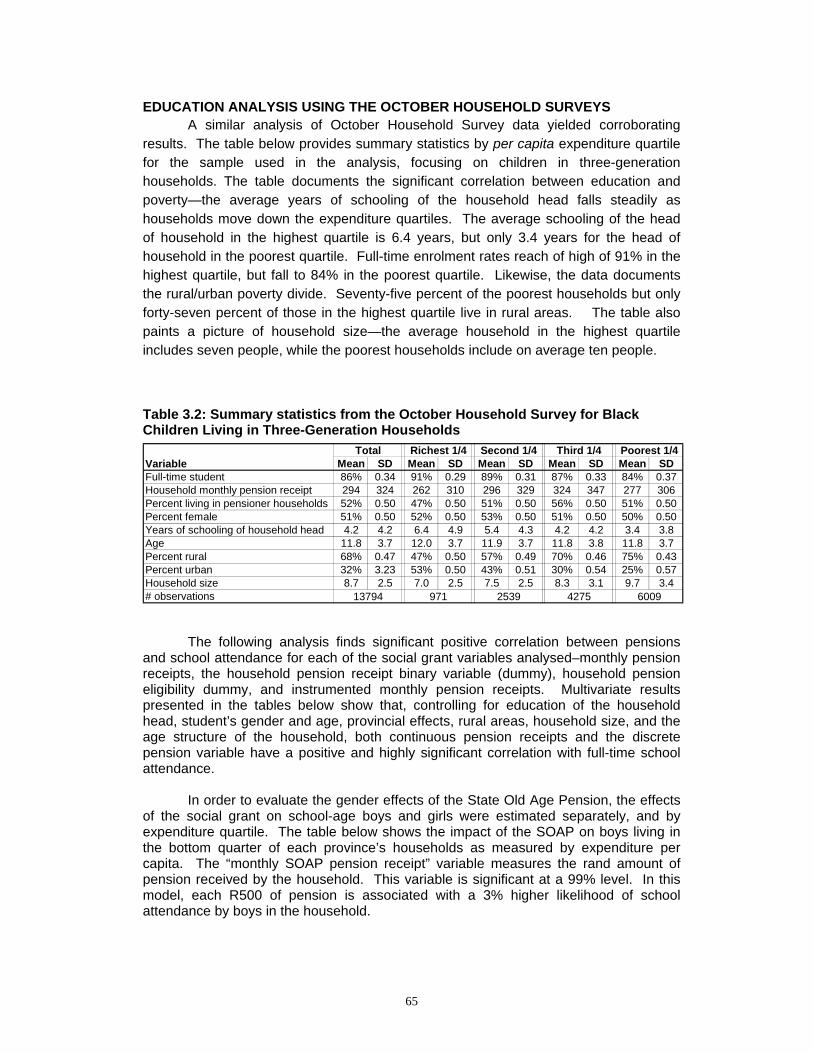
65
EDUCATION ANALYSIS USING THE OCTOBER HOUSEHOLD SURVEYS A similar analysis of October Household Survey data yielded corroborating
results. The table below provides summary statistics by per capita expenditure quartile for the sample used in the analysis, focusing on children in three-generation households. The table documents the significant correlation between education and poverty—the average years of schooling of the household head falls steadily as households move down the expenditure quartiles. The average schooling of the head of household in the highest quartile is 6.4 years, but only 3.4 years for the head of household in the poorest quartile. Full-time enrolment rates reach of high of 91% in the highest quartile, but fall to 84% in the poorest quartile. Likewise, the data documents the rural/urban poverty divide. Seventy-five percent of the poorest households but only forty-seven percent of those in the highest quartile live in rural areas. The table also paints a picture of household size—the average household in the highest quartile includes seven people, while the poorest households include on average ten people. Table 3.2: Summary statistics from the October Household Survey for Black Children Living in Three-Generation Households
The following analysis finds significant positive correlation between pensions and school attendance for each of the social grant variables analysed–monthly pension receipts, the household pension receipt binary variable (dummy), household pension eligibility dummy, and instrumented monthly pension receipts. Multivariate results presented in the tables below show that, controlling for education of the household head, student’s gender and age, provincial effects, rural areas, household size, and the age structure of the household, both continuous pension receipts and the discrete pension variable have a positive and highly significant correlation with full-time school attendance.
In order to evaluate the gender effects of the State Old Age Pension, the effects of the social grant on school-age boys and girls were estimated separately, and by expenditure quartile. The table below shows the impact of the SOAP on boys living in the bottom quarter of each province’s households as measured by expenditure per capita. The “monthly SOAP pension receipt” variable measures the rand amount of pension received by the household. This variable is significant at a 99% level. In this model, each R500 of pension is associated with a 3% higher likelihood of school attendance by boys in the household.
Mean SD Mean SD Mean SD Mean SD Mean SDFull-time student 86% 0.34 91% 0.29 89% 0.31 87% 0.33 84% 0.37Household monthly pension receipt 294 324 262 310 296 329 324 347 277 306Percent living in pensioner households 52% 0.50 47% 0.50 51% 0.50 56% 0.50 51% 0.50Percent female 51% 0.50 52% 0.50 53% 0.50 51% 0.50 50% 0.50Years of schooling of household head 4.2 4.2 6.4 4.9 5.4 4.3 4.2 4.2 3.4 3.8Age 11.8 3.7 12.0 3.7 11.9 3.7 11.8 3.8 11.8 3.7Percent rural 68% 0.47 47% 0.50 57% 0.49 70% 0.46 75% 0.43Percent urban 32% 3.23 53% 0.50 43% 0.51 30% 0.54 25% 0.57Household size 8.7 2.5 7.0 2.5 7.5 2.5 8.3 3.1 9.7 3.4# observations
VariablePoorest 1/4
13794 971 2539 4275 6009
Total Richest 1/4 Second 1/4 Third 1/4
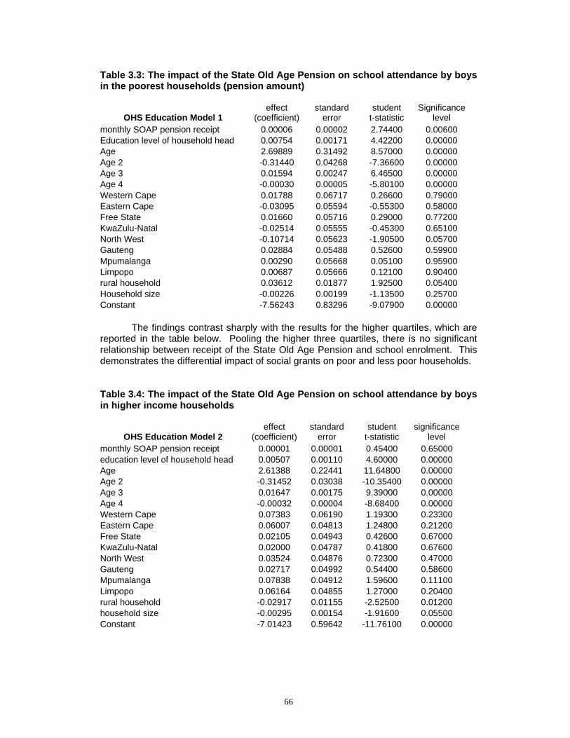
66
Table 3.3: The impact of the State Old Age Pension on school attendance by boys in the poorest households (pension amount)
OHS Education Model 1
effect (coefficient)
standard error
student t-statistic
Significance level
monthly SOAP pension receipt 0.00006 0.00002 2.74400 0.00600 Education level of household head 0.00754 0.00171 4.42200 0.00000 Age 2.69889 0.31492 8.57000 0.00000 Age 2 -0.31440 0.04268 -7.36600 0.00000 Age 3 0.01594 0.00247 6.46500 0.00000 Age 4 -0.00030 0.00005 -5.80100 0.00000 Western Cape 0.01788 0.06717 0.26600 0.79000 Eastern Cape -0.03095 0.05594 -0.55300 0.58000 Free State 0.01660 0.05716 0.29000 0.77200 KwaZulu-Natal -0.02514 0.05555 -0.45300 0.65100 North West -0.10714 0.05623 -1.90500 0.05700 Gauteng 0.02884 0.05488 0.52600 0.59900 Mpumalanga 0.00290 0.05668 0.05100 0.95900 Limpopo 0.00687 0.05666 0.12100 0.90400 rural household 0.03612 0.01877 1.92500 0.05400 Household size -0.00226 0.00199 -1.13500 0.25700 Constant -7.56243 0.83296 -9.07900 0.00000 The findings contrast sharply with the results for the higher quartiles, which are reported in the table below. Pooling the higher three quartiles, there is no significant relationship between receipt of the State Old Age Pension and school enrolment. This demonstrates the differential impact of social grants on poor and less poor households. Table 3.4: The impact of the State Old Age Pension on school attendance by boys in higher income households
OHS Education Model 2
effect (coefficient)
standard error
student t-statistic
significance level
monthly SOAP pension receipt 0.00001 0.00001 0.45400 0.65000 education level of household head 0.00507 0.00110 4.60000 0.00000 Age 2.61388 0.22441 11.64800 0.00000 Age 2 -0.31452 0.03038 -10.35400 0.00000 Age 3 0.01647 0.00175 9.39000 0.00000 Age 4 -0.00032 0.00004 -8.68400 0.00000 Western Cape 0.07383 0.06190 1.19300 0.23300 Eastern Cape 0.06007 0.04813 1.24800 0.21200 Free State 0.02105 0.04943 0.42600 0.67000 KwaZulu-Natal 0.02000 0.04787 0.41800 0.67600 North West 0.03524 0.04876 0.72300 0.47000 Gauteng 0.02717 0.04992 0.54400 0.58600 Mpumalanga 0.07838 0.04912 1.59600 0.11100 Limpopo 0.06164 0.04855 1.27000 0.20400 rural household -0.02917 0.01155 -2.52500 0.01200 household size -0.00295 0.00154 -1.91600 0.05500 Constant -7.01423 0.59642 -11.76100 0.00000
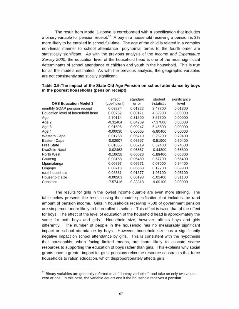
67
The result from Model 1 above is corroborated with a specification that includes a binary variable for pension receipt.32 A boy in a household receiving a pension is 3% more likely to be enrolled in school full-time. The age of the child is related in a complex non-linear manner to school attendance—polynomial terms to the fourth order are statistically significant. As with the previous analysis of the Income and Expenditure Survey 2000, the education level of the household head is one of the most significant determinants of school attendance of children and youth in the household. This is true for all the models estimated. As with the previous analysis, the geographic variables are not consistently statistically significant.
Table 3.5:The impact of the State Old Age Pension on school attendance by boys in the poorest households (pension receipt)
OHS Education Model 3 effect
(coefficient)standard
error student
t-statistic significance
level monthly SOAP pension receipt 0.03274 0.01322 2.47700 0.01300 Education level of household head 0.00752 0.00171 4.39900 0.00000 Age 2.70114 0.31500 8.57500 0.00000 Age 2 -0.31464 0.04269 -7.37000 0.00000 Age 3 0.01596 0.00247 6.46800 0.00000 Age 4 -0.00030 0.00005 -5.80400 0.00000 Western Cape 0.01758 0.06719 0.26200 0.79400 Eastern Cape -0.02907 0.05597 -0.51900 0.60400 Free State 0.01855 0.05719 0.32400 0.74600 KwaZulu-Natal -0.02463 0.05557 -0.44300 0.65800 North West -0.10658 0.05628 -1.89400 0.05800 Gauteng 0.03168 0.05489 0.57700 0.56400 Mpumalanga 0.00397 0.05671 0.07000 0.94400 Limpopo 0.00718 0.05668 0.12700 0.89900 rural household 0.03661 0.01877 1.95100 0.05100 Household size -0.00201 0.00198 -1.01400 0.31100 Constant -7.57416 0.83318 -9.09100 0.00000 The results for girls in the lowest income quartile are even more striking. The table below presents the results using the model specification that includes the rand amount of pension income. Girls in households receiving R500 of government pension are six percent more likely to be enrolled in school. This effect is twice that of the effect for boys. The effect of the level of education of the household head is approximately the same for both boys and girls. Household size, however, affects boys and girls differently. The number of people in the household has no measurably significant impact on school attendance by boys. However, household size has a significantly negative impact on school attendance by girls. This is consistent with the hypothesis that households, when facing limited means, are more likely to allocate scarce resources to supporting the education of boys rather than girls. This explains why social grants have a greater impact for girls: pensions relax the resource constraints that force households to ration education, which disproportionately affects girls. 32 Binary variables are generally referred to as “dummy variables”, and take on only two values—zero or one. In this case, the variable equals one if the household receives a pension.
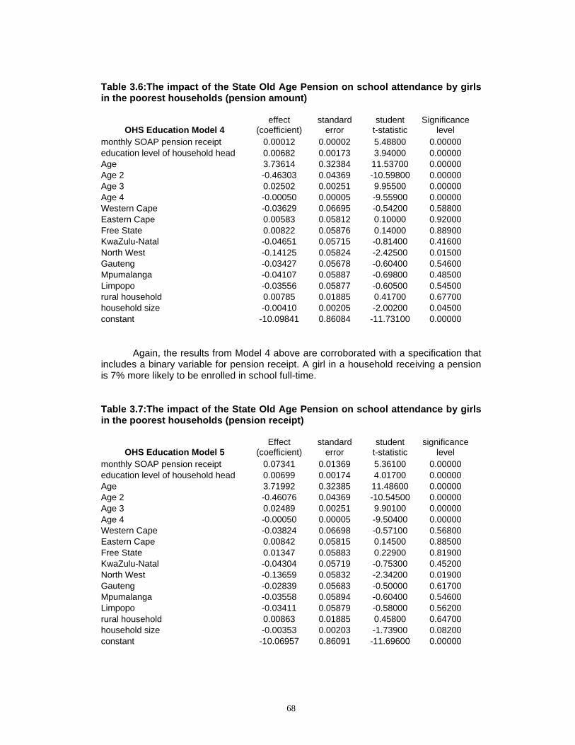
68
Table 3.6:The impact of the State Old Age Pension on school attendance by girls in the poorest households (pension amount)
OHS Education Model 4
effect (coefficient)
standard error
student t-statistic
Significance level
monthly SOAP pension receipt 0.00012 0.00002 5.48800 0.00000 education level of household head 0.00682 0.00173 3.94000 0.00000 Age 3.73614 0.32384 11.53700 0.00000 Age 2 -0.46303 0.04369 -10.59800 0.00000 Age 3 0.02502 0.00251 9.95500 0.00000 Age 4 -0.00050 0.00005 -9.55900 0.00000 Western Cape -0.03629 0.06695 -0.54200 0.58800 Eastern Cape 0.00583 0.05812 0.10000 0.92000 Free State 0.00822 0.05876 0.14000 0.88900 KwaZulu-Natal -0.04651 0.05715 -0.81400 0.41600 North West -0.14125 0.05824 -2.42500 0.01500 Gauteng -0.03427 0.05678 -0.60400 0.54600 Mpumalanga -0.04107 0.05887 -0.69800 0.48500 Limpopo -0.03556 0.05877 -0.60500 0.54500 rural household 0.00785 0.01885 0.41700 0.67700 household size -0.00410 0.00205 -2.00200 0.04500 constant -10.09841 0.86084 -11.73100 0.00000
Again, the results from Model 4 above are corroborated with a specification that includes a binary variable for pension receipt. A girl in a household receiving a pension is 7% more likely to be enrolled in school full-time. Table 3.7:The impact of the State Old Age Pension on school attendance by girls in the poorest households (pension receipt)
OHS Education Model 5
Effect (coefficient)
standard error
student t-statistic
significance level
monthly SOAP pension receipt 0.07341 0.01369 5.36100 0.00000 education level of household head 0.00699 0.00174 4.01700 0.00000 Age 3.71992 0.32385 11.48600 0.00000 Age 2 -0.46076 0.04369 -10.54500 0.00000 Age 3 0.02489 0.00251 9.90100 0.00000 Age 4 -0.00050 0.00005 -9.50400 0.00000 Western Cape -0.03824 0.06698 -0.57100 0.56800 Eastern Cape 0.00842 0.05815 0.14500 0.88500 Free State 0.01347 0.05883 0.22900 0.81900 KwaZulu-Natal -0.04304 0.05719 -0.75300 0.45200 North West -0.13659 0.05832 -2.34200 0.01900 Gauteng -0.02839 0.05683 -0.50000 0.61700 Mpumalanga -0.03558 0.05894 -0.60400 0.54600 Limpopo -0.03411 0.05879 -0.58000 0.56200 rural household 0.00863 0.01885 0.45800 0.64700 household size -0.00353 0.00203 -1.73900 0.08200 constant -10.06957 0.86091 -11.69600 0.00000
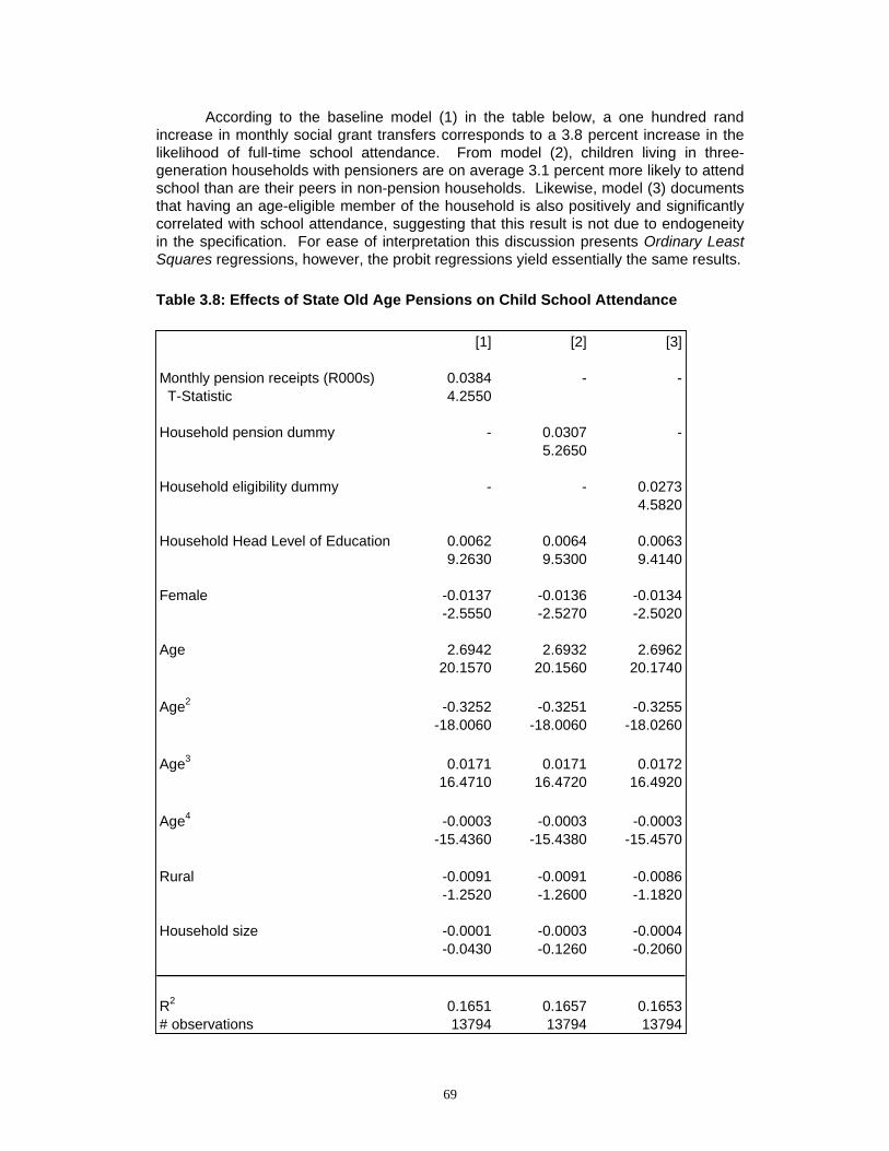
69
According to the baseline model (1) in the table below, a one hundred rand increase in monthly social grant transfers corresponds to a 3.8 percent increase in the likelihood of full-time school attendance. From model (2), children living in three-generation households with pensioners are on average 3.1 percent more likely to attend school than are their peers in non-pension households. Likewise, model (3) documents that having an age-eligible member of the household is also positively and significantly correlated with school attendance, suggesting that this result is not due to endogeneity in the specification. For ease of interpretation this discussion presents Ordinary Least Squares regressions, however, the probit regressions yield essentially the same results. Table 3.8: Effects of State Old Age Pensions on Child School Attendance
[1] [2] [3]
Monthly pension receipts (R000s) 0.0384 - - T-Statistic 4.2550
Household pension dummy - 0.0307 -5.2650
Household eligibility dummy - - 0.02734.5820
Household Head Level of Education 0.0062 0.0064 0.00639.2630 9.5300 9.4140
Female -0.0137 -0.0136 -0.0134-2.5550 -2.5270 -2.5020
Age 2.6942 2.6932 2.696220.1570 20.1560 20.1740
Age2 -0.3252 -0.3251 -0.3255-18.0060 -18.0060 -18.0260
Age3 0.0171 0.0171 0.017216.4710 16.4720 16.4920
Age4 -0.0003 -0.0003 -0.0003-15.4360 -15.4380 -15.4570
Rural -0.0091 -0.0091 -0.0086-1.2520 -1.2600 -1.1820
Household size -0.0001 -0.0003 -0.0004-0.0430 -0.1260 -0.2060
R2 0.1651 0.1657 0.1653# observations 13794 13794 13794
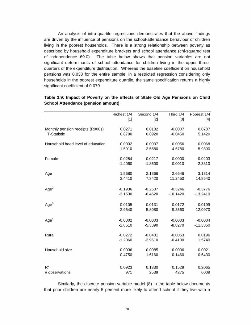
70
An analysis of intra-quartile regressions demonstrates that the above findings are driven by the influence of pensions on the school-attendance behaviour of children living in the poorest households. There is a strong relationship between poverty as described by household expenditure brackets and school attendance (chi-squared test of independence 69.0). The table below shows that pension variables are not significant determinants of school attendance for children living in the upper three-quarters of the expenditure distribution. Whereas the baseline coefficient on household pensions was 0.038 for the entire sample, in a restricted regression considering only households in the poorest expenditure quartile, the same specification returns a highly significant coefficient of 0.079. Table 3.9: Impact of Poverty on the Effects of State Old Age Pensions on Child School Attendance (pension amount)
Similarly, the discrete pension variable model (8) in the table below documents
that poor children are nearly 5 percent more likely to attend school if they live with a
Richest 1/4 Second 1/4 Third 1/4 Poorest 1/4[1] [2] [3] [4]
Monthly pension receipts (R000s) 0.0271 0.0182 -0.0007 0.0787 T-Statistic 0.8790 0.8920 -0.0450 5.1420
Household head level of education 0.0032 0.0037 0.0056 0.00681.5910 2.5580 4.6780 5.9300
Female -0.0254 -0.0217 0.0000 -0.0203-1.4060 -1.8500 0.0010 -2.3810
Age 1.5680 2.1366 2.6646 3.13143.4410 7.3420 11.2450 14.8540
Age2 -0.1936 -0.2537 -0.3246 -0.3776-3.1530 -6.4620 -10.1420 -13.2410
Age3 0.0105 0.0131 0.0172 0.01992.9640 5.8080 9.3560 12.0970
Age4 -0.0002 -0.0003 -0.0003 -0.0004-2.8510 -5.3390 -8.8270 -11.3350
Rural -0.0272 -0.0431 -0.0053 0.0196-1.2060 -2.9610 -0.4130 1.5740
Household size 0.0036 0.0085 -0.0006 -0.00210.4750 1.6160 -0.1460 -0.6430
R2 0.0923 0.1330 0.1529 0.2065# observations 971 2539 4275 6009
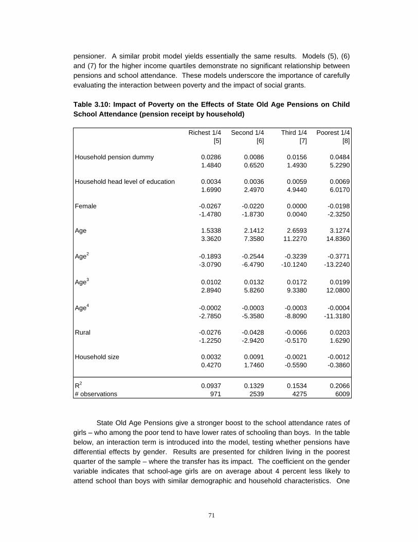
71
pensioner. A similar probit model yields essentially the same results. Models (5), (6) and (7) for the higher income quartiles demonstrate no significant relationship between pensions and school attendance. These models underscore the importance of carefully evaluating the interaction between poverty and the impact of social grants. Table 3.10: Impact of Poverty on the Effects of State Old Age Pensions on Child School Attendance (pension receipt by household)
State Old Age Pensions give a stronger boost to the school attendance rates of girls – who among the poor tend to have lower rates of schooling than boys. In the table below, an interaction term is introduced into the model, testing whether pensions have differential effects by gender. Results are presented for children living in the poorest quarter of the sample – where the transfer has its impact. The coefficient on the gender variable indicates that school-age girls are on average about 4 percent less likely to attend school than boys with similar demographic and household characteristics. One
Richest 1/4 Second 1/4 Third 1/4 Poorest 1/4[5] [6] [7] [8]
Household pension dummy 0.0286 0.0086 0.0156 0.04841.4840 0.6520 1.4930 5.2290
Household head level of education 0.0034 0.0036 0.0059 0.00691.6990 2.4970 4.9440 6.0170
Female -0.0267 -0.0220 0.0000 -0.0198-1.4780 -1.8730 0.0040 -2.3250
Age 1.5338 2.1412 2.6593 3.12743.3620 7.3580 11.2270 14.8360
Age2 -0.1893 -0.2544 -0.3239 -0.3771-3.0790 -6.4790 -10.1240 -13.2240
Age3 0.0102 0.0132 0.0172 0.01992.8940 5.8260 9.3380 12.0800
Age4 -0.0002 -0.0003 -0.0003 -0.0004-2.7850 -5.3580 -8.8090 -11.3180
Rural -0.0276 -0.0428 -0.0066 0.0203-1.2250 -2.9420 -0.5170 1.6290
Household size 0.0032 0.0091 -0.0021 -0.00120.4270 1.7460 -0.5590 -0.3860
R2 0.0937 0.1329 0.1534 0.2066# observations 971 2539 4275 6009
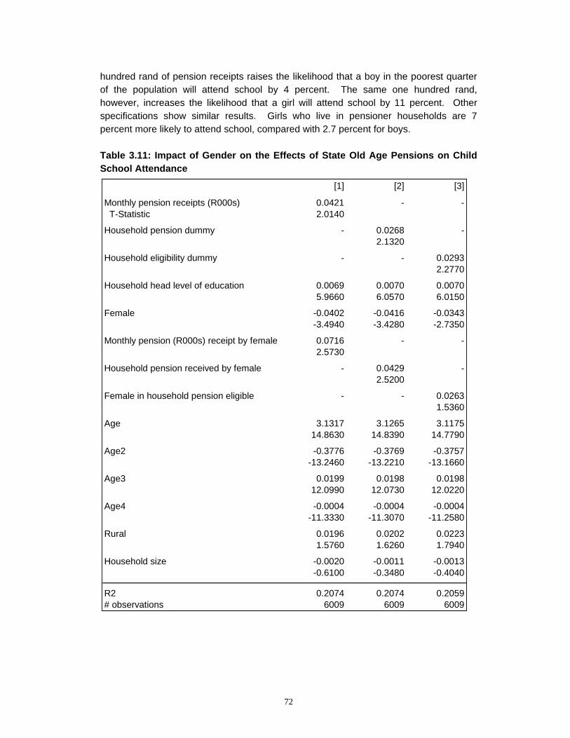
72
hundred rand of pension receipts raises the likelihood that a boy in the poorest quarter of the population will attend school by 4 percent. The same one hundred rand, however, increases the likelihood that a girl will attend school by 11 percent. Other specifications show similar results. Girls who live in pensioner households are 7 percent more likely to attend school, compared with 2.7 percent for boys. Table 3.11: Impact of Gender on the Effects of State Old Age Pensions on Child School Attendance
[1] [2] [3]
Monthly pension receipts (R000s) 0.0421 - - T-Statistic 2.0140
Household pension dummy - 0.0268 -2.1320
Household eligibility dummy - - 0.02932.2770
Household head level of education 0.0069 0.0070 0.00705.9660 6.0570 6.0150
Female -0.0402 -0.0416 -0.0343-3.4940 -3.4280 -2.7350
Monthly pension (R000s) receipt by female 0.0716 - -2.5730
Household pension received by female - 0.0429 -2.5200
Female in household pension eligible - - 0.02631.5360
Age 3.1317 3.1265 3.117514.8630 14.8390 14.7790
Age2 -0.3776 -0.3769 -0.3757-13.2460 -13.2210 -13.1660
Age3 0.0199 0.0198 0.019812.0990 12.0730 12.0220
Age4 -0.0004 -0.0004 -0.0004-11.3330 -11.3070 -11.2580
Rural 0.0196 0.0202 0.02231.5760 1.6260 1.7940
Household size -0.0020 -0.0011 -0.0013-0.6100 -0.3480 -0.4040
R2 0.2074 0.2074 0.2059# observations 6009 6009 6009
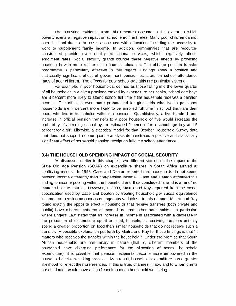
73
The statistical evidence from this research documents the extent to which poverty exerts a negative impact on school enrolment rates. Many poor children cannot attend school due to the costs associated with education, including the necessity to work to supplement family income. In addition, communities that are resource-constrained provide lower quality educational services, which negatively affects enrolment rates. Social security grants counter these negative effects by providing households with more resources to finance education. The old-age pension transfer programme is particularly effective in this regard. Findings show a positive and statistically significant effect of government pension transfers on school attendance rates of poor children. The effects for poor school-age girls are particularly strong.
For example, in poor households, defined as those falling into the lower quarter of all households in a given province ranked by expenditure per capita, school-age boys are 3 percent more likely to attend school full time if the household receives a pension benefit. The effect is even more pronounced for girls: girls who live in pensioner households are 7 percent more likely to be enrolled full time in school than are their peers who live in households without a pension. Quantitatively, a five hundred rand increase in official pension transfers to a poor household of five would increase the probability of attending school by an estimated 2 percent for a school-age boy and 5 percent for a girl. Likewise, a statistical model for that October Household Survey data that does not support income quartile analysis demonstrates a positive and statistically significant effect of household pension receipt on full-time school attendance.
3.4) THE HOUSEHOLD SPENDING IMPACT OF SOCIAL SECURITY
As discussed earlier in this chapter, two different studies on the impact of the State Old Age Pension (SOAP) on expenditure shares in South Africa arrived at conflicting results. In 1998, Case and Deaton reported that households do not spend pension income differently than non-pension income. Case and Deaton attributed this finding to income pooling within the household and thus concluded “a rand is a rand” no matter what the source. However, in 2003, Maitra and Ray departed from the model specification used by Case and Deaton by treating household per capita equivalence income and pension amount as endogenous variables. In this manner, Maitra and Ray found exactly the opposite effect – households that receive transfers (both private and public) have different patterns of expenditure than other households. In particular, where Engel’s Law states that an increase in income is associated with a decrease in the proportion of expenditure spent on food, households receiving transfers actually spend a greater proportion on food than similar households that do not receive such a transfer. A possible explanation put forth by Maitra and Ray for these findings is that “it matters who receives the transfer within the household.” Under the premise that South African households are non-unitary in nature (that is, different members of the household have diverging preferences for the allocation of overall household expenditure), it is possible that pension recipients become more empowered in the household decision-making process. As a result, household expenditure has a greater likelihood to reflect their preferences. If this is true, changes in how and to whom grants are distributed would have a significant impact on household well being.
74
Table 3.12 shows the weighted mean of expenditure shares for households that fall between the twentieth and thirtieth percentile of total household income, the decile in which most of the State Old Age Pensions are concentrated. Table 3.12 Households between the 20th and 30th Percentile of Total Income
Non-Pensioners Pensioners . Expenditure
Category #
Obs. Spending
Share #
Obs. Spending
Share Food 2132 41.3622% 645 43.9445%
Tobacco 693 4.8145% 209 3.1355% Clothing 2132 5.0107% 645 4.4643% Housing 2132 6.8624% 645 6.6656%
Fuel 2132 3.9831% 645 4.7296% Furniture & 2132 1.3922% 645 1.4893% Household 2132 2.7846% 645 3.0373%
Medical Care 2132 0.7253% 645 1.0513% Transportation 2132 3.5489% 645 2.1610% Communication 2132 0.9212% 645 0.9104% Personal Care 2132 5.4028% 645 4.3008%
Holiday 177 0.3130% 38 0.0379% Debt 2132 1.8140% 645 1.1600%
Debt Service 2132 0.0054% 645 0.0003%
Total income 2134 7804 645 7755 SOAP amount 2134 0 645 6421
The average total income of the two groups of households is comparable (R7804 for non-pensioner households versus R7755 for pensioner households. However, the composition of spending is significantly different. The pensioner households spend a larger proportion on food (43.9% versus 41.4%), a smaller proportion on tobacco (3.1% versus 4.8%), less on clothing (4.5% versus 5.0%), more on fuel (4.7% versus 4.0%), more on medical care (1.1% versus 0.7%), less on transportation (2.2% versus 3.5%), less on personal care (4.3% versus 5.4%), and less on holidays (less than 0.1% versus 0.3%). In addition, pensioner households have a lower debt burden and spend less on debt service.
The question arises as to whether these differences can be attributed to the existence of the pension, or whether pension receipt is just a coincidental factor. For pensioner households, the pension income constitutes 83% of total household income. For any given comparison between two variables, there remains the risk that a third factor determines both variables and hence the observed correlation is spurious. For instance, pensioner households spend a higher proportion on medical care. The existence of elderly individuals in the household might explain this relationship—the more elderly individuals, the more likely the household will receive a pension. And the
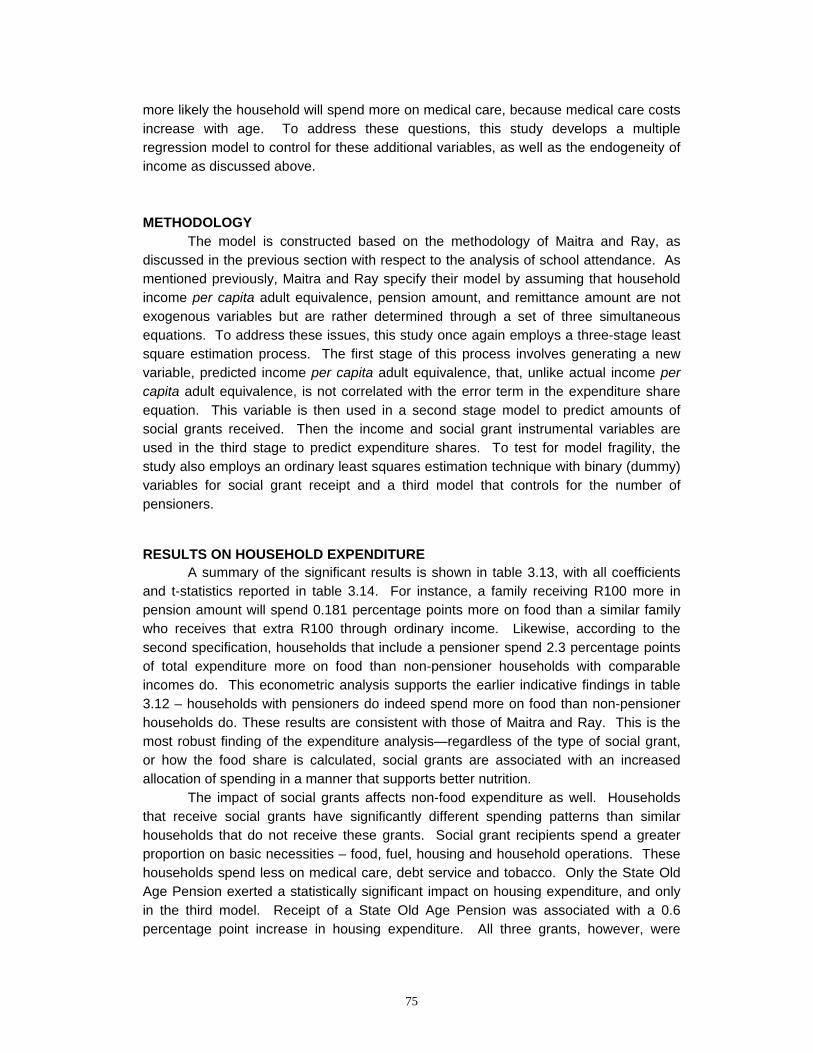
75
more likely the household will spend more on medical care, because medical care costs increase with age. To address these questions, this study develops a multiple regression model to control for these additional variables, as well as the endogeneity of income as discussed above.
METHODOLOGY The model is constructed based on the methodology of Maitra and Ray, as
discussed in the previous section with respect to the analysis of school attendance. As mentioned previously, Maitra and Ray specify their model by assuming that household income per capita adult equivalence, pension amount, and remittance amount are not exogenous variables but are rather determined through a set of three simultaneous equations. To address these issues, this study once again employs a three-stage least square estimation process. The first stage of this process involves generating a new variable, predicted income per capita adult equivalence, that, unlike actual income per capita adult equivalence, is not correlated with the error term in the expenditure share equation. This variable is then used in a second stage model to predict amounts of social grants received. Then the income and social grant instrumental variables are used in the third stage to predict expenditure shares. To test for model fragility, the study also employs an ordinary least squares estimation technique with binary (dummy) variables for social grant receipt and a third model that controls for the number of pensioners.
RESULTS ON HOUSEHOLD EXPENDITURE
A summary of the significant results is shown in table 3.13, with all coefficients and t-statistics reported in table 3.14. For instance, a family receiving R100 more in pension amount will spend 0.181 percentage points more on food than a similar family who receives that extra R100 through ordinary income. Likewise, according to the second specification, households that include a pensioner spend 2.3 percentage points of total expenditure more on food than non-pensioner households with comparable incomes do. This econometric analysis supports the earlier indicative findings in table 3.12 – households with pensioners do indeed spend more on food than non-pensioner households do. These results are consistent with those of Maitra and Ray. This is the most robust finding of the expenditure analysis—regardless of the type of social grant, or how the food share is calculated, social grants are associated with an increased allocation of spending in a manner that supports better nutrition.
The impact of social grants affects non-food expenditure as well. Households that receive social grants have significantly different spending patterns than similar households that do not receive these grants. Social grant recipients spend a greater proportion on basic necessities – food, fuel, housing and household operations. These households spend less on medical care, debt service and tobacco. Only the State Old Age Pension exerted a statistically significant impact on housing expenditure, and only in the third model. Receipt of a State Old Age Pension was associated with a 0.6 percentage point increase in housing expenditure. All three grants, however, were
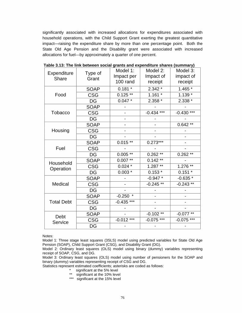
76
significantly associated with increased allocations for expenditures associated with household operations, with the Child Support Grant exerting the greatest quantitative impact—raising the expenditure share by more than one percentage point. Both the State Old Age Pension and the Disability grant were associated with increased allocations for fuel—by approximately a quarter of one percent.
Table 3.13: The link between social grants and expenditure shares (summary)
Expenditure Share
Type of Grant
Model 1: Impact per 100 rand
Model 2: Impact of
receipt
Model 3: impact of receipt
SOAP 0.181 * 2.342 * 1.465 * CSG 0.125 ** 1.161 * 1.139 *
Food
DG 0.047 * 2.358 * 2.338 * SOAP - - - CSG - -0.434 *** -0.430 ***
Tobacco
DG - - - SOAP - - 0.642 ** CSG - - -
Housing
DG - - - SOAP 0.015 ** 0.273*** - CSG - - -
Fuel
DG 0.005 ** 0.262 ** 0.262 ** SOAP 0.007 ** 0.142 ** - CSG 0.024 * 1.287 ** 1.276 **
Household Operation
DG 0.003 * 0.153 * 0.151 * SOAP - -0.947 * -0.635 * CSG - -0.245 ** -0.243 **
Medical
DG - - - SOAP -0.250 * - - CSG -0.435 *** - -
Total Debt
DG - - - SOAP - -0.102 ** -0.077 ** CSG -0.012 *** -0.075 *** -0.075 ***
Debt Service
DG - - - Notes: Model 1: Three stage least squares (3SLS) model using predicted variables for State Old Age Pension (SOAP), Child Support Grant (CSG), and Disability Grant (DG). Model 2: Ordinary least squares (OLS) model using binary (dummy) variables representing receipt of SOAP, CSG, and DG. Model 3: Ordinary least squares (OLS) model using number of pensioners for the SOAP and binary (dummy) variables representing receipt of CSG and DG. Statistics represent estimated coefficients; asterisks are coded as follows:
* significant at the 5% level ** significant at the 10% level *** significant at the 15% level

77
Table 3.14: The link between social grants and expenditure shares (statistics)
Share Grant Model 1 Model 2 Model 3
Pension .0000181 (6.80)*
.0234189 (4.19)*
0.0146481 (3.63)*
Child Support .0000125 (1.73)**
.0116115 (2.43)*
0.0113926 (2.39)*
Food
Disability 4.71e-06 (5.54)*
.0235795 (5.59)*
0.0233758 (5.34)*
Pension -2.74E-07 (-0.18)
.0009697 (0.31)
0.0003817 (0.16)
Child Support -1.73E-06 (-0.39)
-0.00434 (-1.48)***
-0.0042958 (-1.47)***
Tobacco
Disability -5.57E-07 (-1.21)
-0.0027 (-1.14)
-0.0027059 (-1.14)
Pension -1.25E-06 (-0.54)
.0043363 (0.89)
0.00642 (1.82)**
Child Support -4.89E-06 (-0.77)
-0.00285 (-0.68)
-0.002988 (-0.72)
Housing
Disability -2.04E-07 (-0.27)
-0.00104 (-0.27)
-0.0011285 (-0.29)
Pension 1.51E-06 (1.69)**
.0027325 (1.46)***
0.0013585 (1.00)
Child Support 1.62E-06 (0.67)
0.001985 (1.24)
0.0019955 (1.25)
Fuel
Disability 5.04E-07 (1.77)**
0.002622 (1.79)**
0.0026208 (1.79)**
Pension 7.19e-07 (1.86)**
.0014257 (1.76)**
.0008013 (1.37)
Child Support 2.35e-06 (2.23)*
.0012866 (1.86)**
.0012764 (1.84)**
Household Operation
Disability 3.05e-07 (2.47)*
.0015263 (2.4)*
.0015144 (2.38)*
Pension 1.05E-07 (0.13)
-.0094714 (-5.74)*
-0.0063468 (-5.32)*
Child Support -2.91E-06 (-1.35)
-0.00245 (-1.74)**
-0.0024252 (-1.72)**
Medical
Disability 2.12E-07 (0.84)
0.001457 (1.13)
0.0015237 (1.18)
Pension -.000025 (-2.37)*
-.0240303 (-1.08)
.0076321 (0.48)
Child Support -.0000435 (-1.51)***
-.0225156 (-1.19)
-.0228754 (-1.21)
Debt Disability -2.43e-06
(-0.72)-.0117609
(-0.68)-.0117574
(-0.68) Pension -1.76e-07
(-0.61)-.0010222 (-1.69)**
-.0007764 (-1.78)**
Child Support -1.21e-06 (-1.55)***
-.0007533 (-1.46)***
-.0007549 (-1.47)***
Debt Service
Disability -9.82e-08 (-1.07)
-.0004905 (-1.04)
-.0004864 (-1.03)
(First number represents coefficient estimate, below that is the calculated t-statistic.)
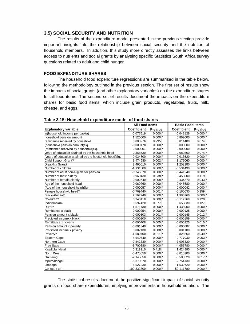
78
3.5) SOCIAL SECURITY AND NUTRITION The results of the expenditure model presented in the previous section provide
important insights into the relationship between social security and the nutrition of household members. In addition, this study more directly assesses the links between access to nutrients and social grants by analysing specific Statistics South Africa survey questions related to adult and child hunger.
FOOD EXPENDITURE SHARES
The household food expenditure regressions are summarised in the table below, following the methodology outlined in the previous section. The first set of results show the impacts of social grants (and other explanatory variables) on the expenditure shares for all food items. The second set of results document the impacts on the expenditure shares for basic food items, which include grain products, vegetables, fruits, milk, cheese, and eggs.
Table 3.15: Household expenditure model of food shares
The statistical results document the positive significant impact of social security
grants on food share expenditures, implying improvements in household nutrition. The
Explanatory variable Coefficient Coefficientln(household income per capita) -0.077619 0.000 * -0.045139 0.000 *household pension amount 1.520000 0.000 * 0.869000 0.000 *remittance received by household 0.000276 0.995 0.011400 0.674 (household pension amount)Sq. -0.000178 0.000 * 0.000000 0.000 *(remittance received by household)Sq. -0.000001 0.000 * 0.000000 0.000 *years of education attained by the household head 0.368630 0.000 * 0.080860 0.074 *(years of education attained by the household head)Sq. -0.034800 0.000 * -0.013520 0.000 *Child Support Grant? 1.474980 0.002 * 1.177060 0.000 *Disability Grant? 2.495010 0.000 * 1.252380 0.000 *Number of children -1.131300 0.000 * -0.531490 0.000 *Number of adult non-eligible for pension -0.745570 0.000 * -0.441240 0.000 *Number of male elderly 0.960430 0.038 * 0.458000 0.119 Number of female elderly -0.902540 0.008 * -0.434370 0.043 *Age of the household head -0.060260 0.000 * -0.046580 0.000 *(Age of the household head)Sq. 0.000057 0.000 * 0.000042 0.000 *Female household head? -0.769440 0.001 * -0.160630 0.259 Black/African? 2.567240 0.000 * 1.985260 0.000 *Coloured? 3.343110 0.000 * -0.117260 0.720 Indian/Asian? 0.597420 0.377 -0.653830 0.127 Rural? 1.571730 0.000 * 1.438900 0.000 *Remittance x black 0.000254 0.000 * 0.000125 0.000 *Pension amount x black -0.000303 0.001 * -0.000145 0.012 *Predicted income x black -0.000200 0.000 * -0.000159 0.000 *Remittance x poverty -0.000408 0.005 * -0.000225 0.015 *Pension amount x poverty -0.001340 0.000 * -0.000887 0.000 *Predicted income x poverty 0.002130 0.000 * 0.001100 0.000 *Poverty? -1.680700 0.011 * -0.826660 0.049 *Eastern Cape -4.640740 0.000 * -0.777930 0.003 *Northern Cape -2.842830 0.000 * -3.008320 0.000 *Free State -8.700380 0.000 * -4.056780 0.000 *KwaZulu_Natal 0.318310 0.418 1.424990 0.000 *North West -5.475550 0.000 * -3.015200 0.000 *Gautemg -2.145050 0.000 * -0.588320 0.017 *Mpumalanga -5.370670 0.000 * -2.754130 0.000 *Limpopo -5.527330 0.000 * -1.530720 0.000 *Constant term 102.332300 0.000 * 59.111780 0.000 *
P-value P-valueAll Food Items Basic Food Items
79
coefficient on the State Old Age Pension indicates that each thousand rand of annual pension receipt is associated with an increase of 1.5 percentage points in the share of household spending on all food items, and an increase nearly one percentage point in the share of spending on basic food items. Likewise, receipt of a Child Support Grant was associated with an increase of 1.5 percentage points in the share of household spending on all food items, and an increase of 1.2 percentage points in the share of spending on basic food items. Similarly, receipt of a Disability Grant was associated with an increase of 2.5 percentage points in the share of household spending on all food items, and an increase of 1.3 percentage points in the share of spending on basic food items. These results are all statistically significant at a 99% level.
The coefficients on household income document that expenditure shares for
both all food items and basic food items tend to decline as households receive more non-grant income. This finding is consistent with results generally obtained in household expenditure models for other countries. The income effects may be interacting with geographic variables included in the analysis. The provincial and rural/urban variables in the model are statistically significant in nearly every case, documenting the important variation in different parts of the country. For example, the average expenditure share on food in rural areas, where the median income is relatively low, is 1.5 percentage points higher than that in urban areas. This may reflect problems with the specification of income in the model, or alternatively a relatively lower price for food in rural areas which results in expenditure substitution. The model was also estimated for each province, and the provincial results are presented in the table below. Table 3.16: Food share household expenditure model by province
The statistical significance is weaker at a provincial level because the sample sizes for each regression are smaller. Nevertheless, all the significant results corroborate the national findings. For each province, higher non-grant income is
Province Statistic Income
State Old Age
Pension
Child Support
GrantDisability
Grant Remittances EducationWestern Cape Coefficient -0.10027 0.00000 0.03743 0.03009 0.00000 0.01091
P-value 0.00000 0.68700 0.00600 0.01100 0.37700 0.00000
Eastern Cape Coefficient -0.07856 0.00002 -0.00174 0.02454 0.00001 0.00856P-value 0.00000 0.00000 0.90700 0.02400 0.00300 0.00000
Northern Cape Coefficient -0.09225 0.00001 0.00560 0.03877 0.00000 0.00815P-value 0.00000 0.09300 0.73000 0.00200 0.08000 0.01200
Free State Coefficient -0.03552 0.00000 0.00783 0.02973 0.00001 0.00168P-value 0.00200 0.63100 0.69600 0.06700 0.00400 0.51500
KwaZulu-Natal Coefficient -0.05946 0.00002 0.03501 0.00305 0.00000 0.00043P-value 0.00000 0.00000 0.00700 0.77400 0.03000 0.78600
North West Coefficient -0.05482 0.00001 0.00971 0.02784 0.00000 0.00126P-value 0.00000 0.06000 0.57400 0.06200 0.22200 0.57700
Gauteng Coefficient -0.05646 0.00001 0.03489 -0.00199 0.00000 0.00305P-value 0.00000 0.03300 0.01400 0.90200 0.90700 0.17400
Mpumalanga Coefficient -0.05264 0.00002 0.00935 0.02156 0.00000 0.00113P-value 0.00000 0.01300 0.38000 0.14600 0.58900 0.57900
Limpopo Coefficient -0.05121 0.00001 0.00638 0.02662 0.00000 0.00308P-value 0.00000 0.05100 0.65400 0.07900 0.70600 0.15800

80
negatively and statistically significantly associated with lower expenditure shares on food. All statistically significant findings for social grants yield positive correlations between all the social grant variables and the expenditure share on food. Likewise, a greater amount of remittances and more years of schooling of the household head are associated with higher expenditure shares on food, controlling for the effect of income. HUNGER
In order to test the results of the expenditure model, this study analysed adult and child hunger as direct measures correlated with nutritional status. In the household section of the September 2000 Labour Force Survey, Statistics South Africa captured information about how many children and adults experienced hunger in the previous year because of insufficient money to buy food. This data supports the analysis of hunger using the same methodology adopted for education. This study follows the Statistics South Africa survey question, defining adult hunger as a binary variable equal to one if the household reported an adult or older child suffering from hunger in the previous year because of insufficient money to buy food. Likewise, child hunger is measured as a binary variable equal to one if the household reported a young child (under seven years of age) suffering from hunger in the previous year because of insufficient money to buy food. The table below presents summary statistics on the
prevalence of hunger in households by province. Nationally, nearly one in five households have experienced hunger over the past year. The highest income provinces—Gauteng and the Western Cape—have the lowest prevalence rates of hunger (13.58% and 10.41% respectively). The prevalence rate of hunger is highest in one of South Africa’s poorest provinces—nearly one in three households in the Eastern Cape experiences hunger. However, another of the poorest provinces—Limpopo—has a hunger prevalence rate of only 14.59%, the third lowest in the country. Meanwhile, Mpumalanga—with a poverty rate below the national average—has the second highest hunger prevalence rate in the country.
This study estimated four models to explain these variables, using the same set
of explanatory variables employed for the education household expenditure analysis. The first two models focus on adult (and older child) hunger, first across all households and second with a sample limited to low income households. The second set of models analyses young child hunger, again first with all households and second with the sample restricted to low income households. These models focus on the State Old Age Pension because of its large rand value and high rate of take-up in the sample. The pension variables included in the model are the number of female and number of male pensioners in the household, providing an assessment of gender impacts. In addition, the study focuses on the interaction between geographical variables and the other key
% of households experiencing
hungerNational 19.36%Western Cape 10.41%Eastern Cape 30.54%Northern Cape 14.31%Free State 23.33%KwaZulu-Natal 19.01%North West 20.89%Gauteng 13.58%Mpumalanga 28.79%Limpopo 14.59%
Table 3.17: Prevalence of hunger in households
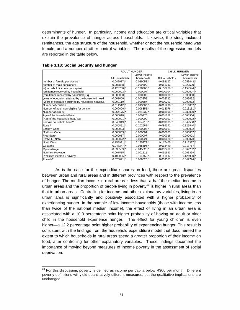
81
determinants of hunger. In particular, income and education are critical variables that explain the prevalence of hunger across households. Likewise, the study included remittances, the age structure of the household, whether or not the household head was female, and a number of other control variables. The results of the regression models are reported in the table below. Table 3.18: Social Security and hunger
As is the case for the expenditure shares on food, there are great disparities
between urban and rural areas and in different provinces with respect to the prevalence of hunger. The median income in rural areas is less than a half the median income in urban areas and the proportion of people living in poverty33 is higher in rural areas than that in urban areas. Controlling for income and other explanatory variables, living in an urban area is significantly and positively associated with a higher probability of experiencing hunger. In the sample of low income households (those with income less than twice of the national median income), the effect of living in an urban area is associated with a 10.3 percentage point higher probability of having an adult or older child in the household experience hunger. The effect for young children is even higher—a 12.2 percentage point higher probability of experiencing hunger. This result is consistent with the findings from the household expenditure model that documented the extent to which households in rural areas spend a greater proportion of their income on food, after controlling for other explanatory variables. These findings document the importance of moving beyond measures of income poverty in the assessment of social deprivation.
33 For this discussion, poverty is defined as income per capita below R300 per month. Different poverty definitions will yield quantitatively different measures, but the qualitative implications are unchanged.
number of female pensioners -0.042917 * -0.039058 * -0.058197 * -0.053443 *number of male pensioners 0.007888 0.009690 0.011313 0.022590ln(household income per capita) -0.126760 * -0.138360 * -0.136768 * -0.154544 *remittance received by household -0.000003 * -0.000004 -0.000004 * -0.000007 *(remittance received by household)Sq. 0.000000 0.000000 0.000000 * 0.000000years of education attained by the household head -0.002606 -0.003358 0.002712 0.002032(years of education attained by household head)Sq. 0.000119 0.000387 -0.000293 0.000062Number of children -0.014512 * -0.013609 * -0.011798 * -0.013852 *Number of adult non-eligible for pension -0.009606 * -0.008355 * -0.013076 * -0.013151 *Number of elderly -0.064175 * -0.071639 * -0.063998 * -0.080050 *Age of the household head 0.000018 0.000278 -0.001152 * -0.000904(Age of the household head)Sq. 0.000001 * 0.000000 0.000002 * 0.000002 *Female household head? -0.043319 * -0.054913 * -0.039335 * -0.049558 *Rural? -0.080881 * -0.102689 * -0.095141 * -0.121840 *Eastern Cape -0.000003 -0.000006 * 0.000001 -0.000002Northern Cape -0.000003 * -0.000004 -0.000003 -0.000007 *Free State -0.000017 -0.000007 -0.000016 -0.000001KwaZulu_Natal -0.000022 * -0.000021 -0.000020 * -0.000023 North West 0.155931 * 0.155372 * 0.117405 * 0.116337 *Gautemg 0.043347 * 0.065695 * 0.018440 0.013767 Mpumalanga -0.038539 * -0.045628 * -0.052409 * -0.069282 *Northern Province -0.007515 0.001811 -0.051953 * -0.068339 Predicted income x poverty -0.103096 * -0.104753 * -0.111112 * -0.126930 *Poverty? 0.070091 * 0.058626 * 0.053501 * 0.049724 *
ADULT HUNGER CHILD HUNGERLower Income
householdsAll HouseholdsLower Income
householdsAll Households
82
All four models above indicate significantly negative coefficients for the number of female pensioners in the household. The coefficients for the number of male pensioners are not significantly different from zero. The size of the impact of female pensioners is greater for children than for adults. An additional female pensioner in the household is associated with a 5.8% lower probability of a young child in the household experiencing hunger, and a 4.3% lower probability for adults and older children. (Restricting the sample to lower income households, an additional female pensioner in the household is associated with a 5.3% lower probability of a young child in the household experiencing hunger, and a 3.9% lower probability for adults and older children.) The consistent significance of female pensioners in the face or persistent statistical insignificance of male pensioners raises the question of the gender impact of social security receipt.
A gender decomposition of the pension effect on food expenditure shares and
hunger demonstrates that the number of male pensioners is significantly associated with an increased household expenditure share on food but no impact in terms of reducing hunger. The number of female pensioners has the opposite correlation—significantly lower prevalence rates of hunger but no effect on food expenditure shares. These statistical results are consistent with the theory of the non-unitary household—in this case that increases in household expenditure shares on food do not necessarily benefit the nutritional status of all members in the household. In other words, male pensioners may be spending their pension income on food for themselves, rather than for other members of the household. Female pensioners, on the other hand, may allocate more resources to other household members, particularly young children.
Remittances are another income source that significantly reduces adult and
child hunger. The quantitative impact is relatively small compared to the effect of female pensioners—an extra R100 of remittance income received by the household is associated with a 0.03% reduction in the probability of an adult or older child experiencing hunger. This effect is more than twice as strong for young children in low income households.
3.6) SOCIAL SECURITY AND HEALTH The results of the expenditure model presented in the section 3.4 also provide
some insights into the relationship between social security and the health status of household members. The household medical expenditure regressions are summarised in the table below, following the methodology previously employed. Two models are estimated—one which includes among the explanatory variables the rand amount of State Old Age Pension, and the other that includes the number of pensioners in the household. In addition, the models include indicators of whether or not the households receive the Child Support Grant or the Disability Grant. The model involves a two-stage process to control for the endogeneity of income—predicting income based on the exogenous variables in the model and using the predicted income to explain the medical shares of total expenditure. In addition, the study focuses on the interaction between
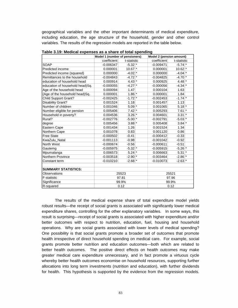
83
geographical variables and the other important determinants of medical expenditure, including education, the age structure of the household, gender and other control variables. The results of the regression models are reported in the table below. Table 3.19: Medical expenses as a share of total spending
The results of the medical expense share of total expenditure model yields robust results—the receipt of social grants is associated with significantly lower medical expenditure shares, controlling for the other explanatory variables. In some ways, this result is surprising—receipt of social grants is associated with higher expenditure and/or better outcomes with respect to nutrition, education, fuel, housing and household operations. Why are social grants associated with lower levels of medical spending? One possibility is that social grants promote a broader set of outcomes that promote health irrespective of direct household spending on medical care. For example, social grants promote better nutrition and education outcomes—both which are related to better health outcomes. The positive direct effects on health outcomes may make greater medical care expenditure unnecessary, and in fact promote a virtuous cycle whereby better health outcomes economise on household resources, supporting further allocations into long term investments (nutrition and education), with further dividends for health. This hypothesis is supported by the evidence from the regression models.
coefficient coefficientSOAP -0.006347 -5.32 * -0.009471 -5.74 *Predicted income 0.000001 10.67 * 0.000001 10.62 *Predicted income (squared) 0.000000 -4.02 * 0.000000 -4.04 *Remittances to the household -0.004843 -4.72 * -0.004825 -4.70 *education of household head 0.000914 4.43 * 0.000925 4.48 *education of household head)Sq. -0.000055 -4.27 * -0.000056 -4.34 *Age of the household head 0.000094 1.47 0.000104 1.63(Age of the household head)Sq. 0.000001 1.86 * 0.000001 1.84Child Support Grant? -0.002425 -1.72 * -0.002453 -1.74 *Disability Grant? 0.001524 1.18 0.001457 1.13Number of children 0.001046 5.09 * 0.001065 5.18 *Number eligible for pension 0.005406 7.42 * 0.005293 7.61 *Household in poverty? 0.004536 3.26 * 0.004601 3.31 *Rural? -0.002776 -5.00 * -0.002791 -5.03 *degree 0.005456 3.88 * 0.005408 3.84 *Eastern Cape 0.001434 1.26 0.001524 1.34Northern Cape 0.001078 0.83 0.001120 0.86Free State -0.000502 -0.41 -0.000412 -0.33KwaZulu_Natal -0.001113 -0.98 -0.001042 -0.92North West -0.000674 -0.56 -0.000611 -0.51Gautemg -0.005975 -5.32 * -0.005915 -5.26 *Mpumalanga 0.006573 5.24 * 0.006663 5.31 *Northern Province -0.003518 -2.90 * -0.003464 -2.86 *Constant term -0.010210 -2.68 * -0.010073 -2.63 *
SUMMARY STATISTICS:ObservationsF-statisticSignificanceR-squared
Model 1 (number of pensioners)t-statistic t-statistic
Model 2 (pension amount)
2552197.9699.9%0.12
2552397.8199.9%0.12
84
For instance, the number of people in the household eligible for the pension is positively associated with greater medical care expenditure. This is not surprising, since medical expenses tend to increase with age. However, the number of people receiving pensions is negatively associated with medical care expenditure. This is consistent with the finding that pension income supports positive health outcomes that reduce the necessity of medical care expenditure.
One important outcome may result from improved education, and the health implications may be substantial. Not only does increasing school attendance among poor children add to human capital, improving future productivity and prospects for economic growth; it also exerts an important long-term effect by stemming the spread of HIV/AIDS. The World Bank notes that increasing education, and in particular the education of women, is one of the most effective ways to combat the spread of HIV/AIDS:
“An increased level of education provides young girls with earning power to enhance their economic independence, which may keep them from resorting to commercial sex work for economic survival, thereby reducing their risk of HIV infection. Education also provides girls with the confidence and the basic knowledge to make sound decisions about their sexual health, again reducing their risk of contracting HIV. Increased efforts in girls’ education are needed now because young girls are disproportionately infected and affected by this epidemic and by the many other reproductive health problems they face, such as female genital mutilation and unwanted pregnancy. Not only are they being infected with HIV, they are being pulled out of school to care for sick relatives or assume family responsibilities as their parents die. Efforts to increase girls’ education should take these problems into account and find solutions to them.”34
3.7) OTHER SOCIAL INDICATORS This study has focused on the relationship between social security and the main objectives of social investment—health, education and nutrition. In addition, the results of the expenditure model presented in the section 3.4 also provide insights into other indicators of well-being. For example, receipt of the Child Support Grant is associated with a lower household expenditure share on tobacco, even controlling for the number of children in the household. Likewise, receipt of social grants is associated with a lower household spending share on tobacco, alcohol and gambling. In addition, households that receive social grants have lower household indebtedness and smaller debt service burdens, controlling for household income and other explanatory variables. The positive implications of the household expenditure models are corroborated by direct tests of the relationship between social grants and social indicators, where data is available. For instance, the September 2000 Labour Force Survey captured a number of measures of household well-being related to access to water and sanitation. One important variable is the prevalence of piped water, measured in binary form with a value of one if the household has access to piped water. The table below presents the results of a regression of this measure on explanatory variables such as receipt of social 34 World Bank (1999).
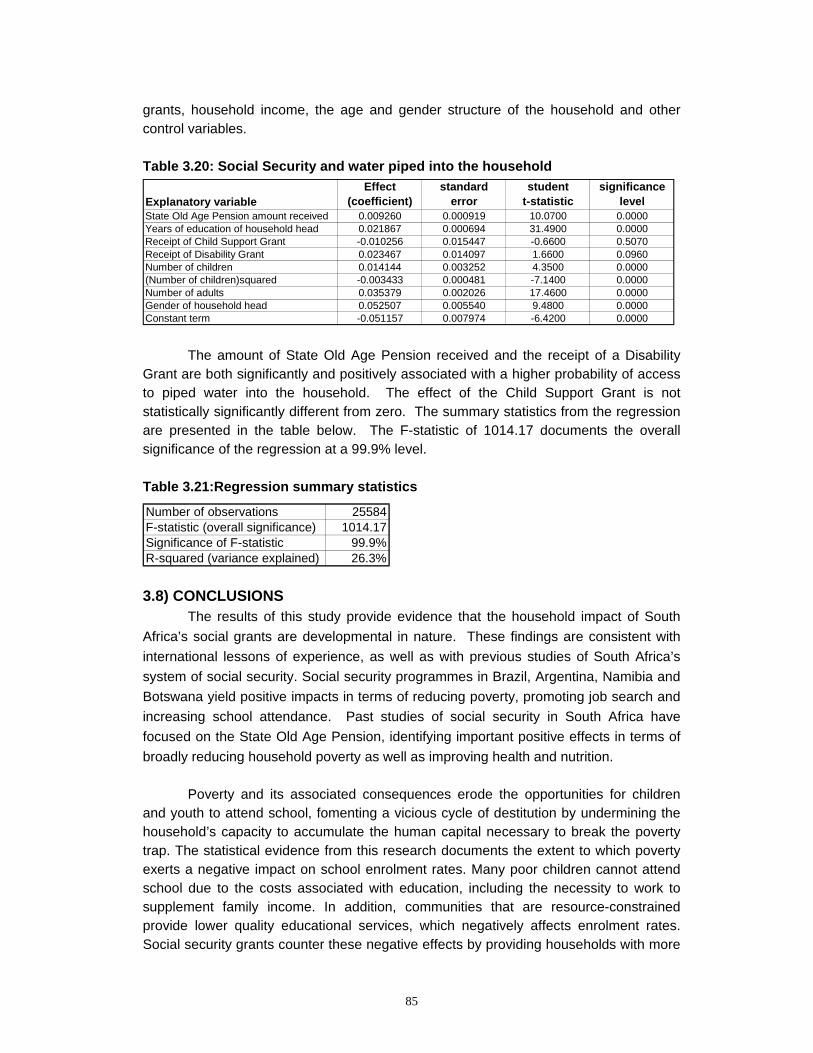
85
grants, household income, the age and gender structure of the household and other control variables. Table 3.20: Social Security and water piped into the household
The amount of State Old Age Pension received and the receipt of a Disability Grant are both significantly and positively associated with a higher probability of access to piped water into the household. The effect of the Child Support Grant is not statistically significantly different from zero. The summary statistics from the regression are presented in the table below. The F-statistic of 1014.17 documents the overall significance of the regression at a 99.9% level. Table 3.21:Regression summary statistics
3.8) CONCLUSIONS
The results of this study provide evidence that the household impact of South Africa’s social grants are developmental in nature. These findings are consistent with international lessons of experience, as well as with previous studies of South Africa’s system of social security. Social security programmes in Brazil, Argentina, Namibia and Botswana yield positive impacts in terms of reducing poverty, promoting job search and increasing school attendance. Past studies of social security in South Africa have focused on the State Old Age Pension, identifying important positive effects in terms of broadly reducing household poverty as well as improving health and nutrition.
Poverty and its associated consequences erode the opportunities for children
and youth to attend school, fomenting a vicious cycle of destitution by undermining the household’s capacity to accumulate the human capital necessary to break the poverty trap. The statistical evidence from this research documents the extent to which poverty exerts a negative impact on school enrolment rates. Many poor children cannot attend school due to the costs associated with education, including the necessity to work to supplement family income. In addition, communities that are resource-constrained provide lower quality educational services, which negatively affects enrolment rates. Social security grants counter these negative effects by providing households with more
Number of observations 25584F-statistic (overall significance) 1014.17Significance of F-statistic 99.9%R-squared (variance explained) 26.3%
Explanatory variableEffect
(coefficient)standard
errorstudent
t-statisticsignificance
levelState Old Age Pension amount received 0.009260 0.000919 10.0700 0.0000Years of education of household head 0.021867 0.000694 31.4900 0.0000Receipt of Child Support Grant -0.010256 0.015447 -0.6600 0.5070Receipt of Disability Grant 0.023467 0.014097 1.6600 0.0960Number of children 0.014144 0.003252 4.3500 0.0000(Number of children)squared -0.003433 0.000481 -7.1400 0.0000Number of adults 0.035379 0.002026 17.4600 0.0000Gender of household head 0.052507 0.005540 9.4800 0.0000Constant term -0.051157 0.007974 -6.4200 0.0000
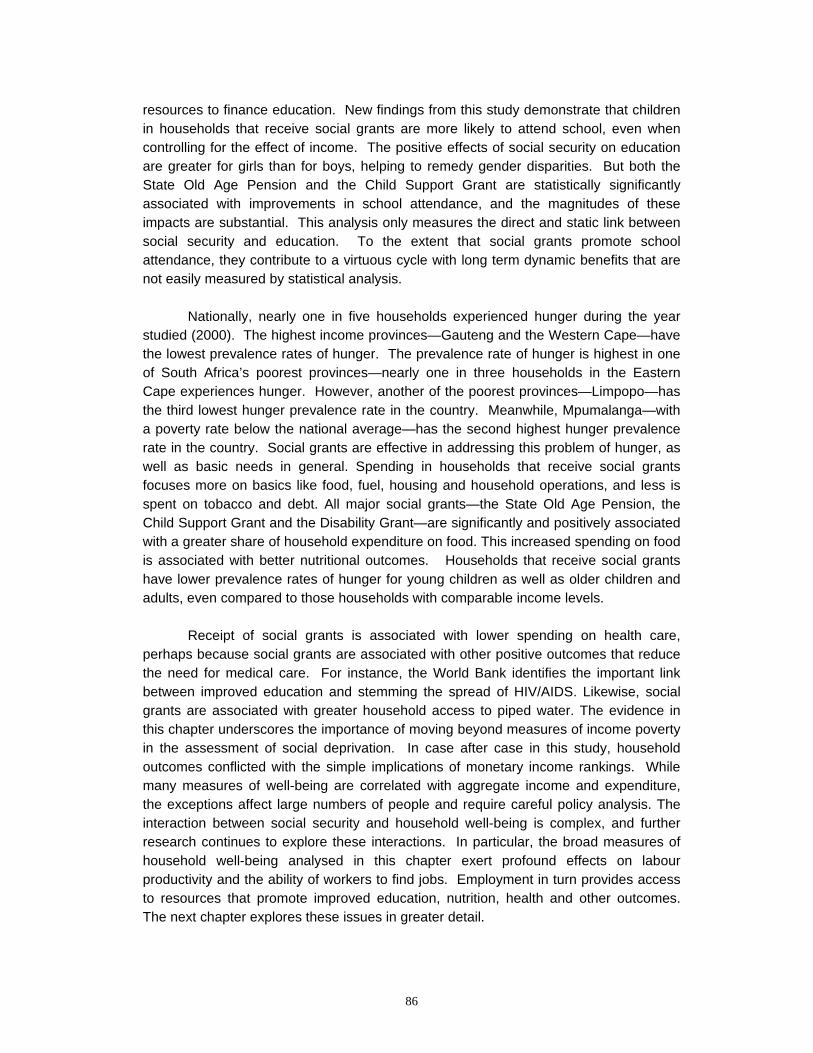
86
resources to finance education. New findings from this study demonstrate that children in households that receive social grants are more likely to attend school, even when controlling for the effect of income. The positive effects of social security on education are greater for girls than for boys, helping to remedy gender disparities. But both the State Old Age Pension and the Child Support Grant are statistically significantly associated with improvements in school attendance, and the magnitudes of these impacts are substantial. This analysis only measures the direct and static link between social security and education. To the extent that social grants promote school attendance, they contribute to a virtuous cycle with long term dynamic benefits that are not easily measured by statistical analysis.
Nationally, nearly one in five households experienced hunger during the year
studied (2000). The highest income provinces—Gauteng and the Western Cape—have the lowest prevalence rates of hunger. The prevalence rate of hunger is highest in one of South Africa’s poorest provinces—nearly one in three households in the Eastern Cape experiences hunger. However, another of the poorest provinces—Limpopo—has the third lowest hunger prevalence rate in the country. Meanwhile, Mpumalanga—with a poverty rate below the national average—has the second highest hunger prevalence rate in the country. Social grants are effective in addressing this problem of hunger, as well as basic needs in general. Spending in households that receive social grants focuses more on basics like food, fuel, housing and household operations, and less is spent on tobacco and debt. All major social grants—the State Old Age Pension, the Child Support Grant and the Disability Grant—are significantly and positively associated with a greater share of household expenditure on food. This increased spending on food is associated with better nutritional outcomes. Households that receive social grants have lower prevalence rates of hunger for young children as well as older children and adults, even compared to those households with comparable income levels.
Receipt of social grants is associated with lower spending on health care,
perhaps because social grants are associated with other positive outcomes that reduce the need for medical care. For instance, the World Bank identifies the important link between improved education and stemming the spread of HIV/AIDS. Likewise, social grants are associated with greater household access to piped water. The evidence in this chapter underscores the importance of moving beyond measures of income poverty in the assessment of social deprivation. In case after case in this study, household outcomes conflicted with the simple implications of monetary income rankings. While many measures of well-being are correlated with aggregate income and expenditure, the exceptions affect large numbers of people and require careful policy analysis. The interaction between social security and household well-being is complex, and further research continues to explore these interactions. In particular, the broad measures of household well-being analysed in this chapter exert profound effects on labour productivity and the ability of workers to find jobs. Employment in turn provides access to resources that promote improved education, nutrition, health and other outcomes. The next chapter explores these issues in greater detail.
87
CHAPTER 4) The Labour Market Impact of Social Assistance Programmes 4.1) INTRODUCTION
This chapter evaluates the impact of South Africa’s social development grants on labour market activity, identifying theoretically and empirically the impact of the social security programmes in terms of labour demand and supply. This research builds on the household impact assessment in the previous chapter, quantifying those factors that affect worker productivity and consequently employer demand for labour. In addition, the study assesses the incentive effects of social grants and their impact on labour force participation. Taken together, these two dimensions of the analysis provide evidence identifying the net impact of social grants on job creation in South Africa.
This chapter consists of four major sections. The first section (4.2) examines the theoretical and empirical literature on linkages between social security and labour markets, with a specific focus on South African evidence. The second section of the chapter (4.3) analyses the labour supply effects resulting from social development grants. Section 4.4 analyses the demand side of the labour market, evaluating the impact of social grants on wages and implicitly the productivity of labour. The final section (4.5) evaluates and summarises the policy implications of the findings. 4.2) LITERATURE REVIEW Bhorat and Leibbrandt (2001) provide an excellent analysis of the broad issues affecting poverty and the South African labour market. They examine the question of the voluntary versus involuntary nature of unemployment: are the unemployed jobless because they prefer to consume additional leisure in favour of taking a job at the market wage, or are they willing to work at the market wage but unable to find employment. Evidence documents the involuntary nature of unemployment in South Africa. Kingdon and Knight (2000) find little support for the classification of most South African unemployment as voluntary, as the unemployed are substantially worse off than even the informally employed on a broad range of indicators, including income and well-being. They hypothesise that there are barriers to entry to the informal or self-employment sector (whose participants are significantly more satisfied with the quality of their lives).
There also continues to be a debate over the appropriate definition for labour
force participation (and therefore, unemployment rates). There are two competing definitions of labour force participation, broad and narrow. The narrow definition of participation excludes discouraged workers—those that would accept a job if offered but do not engage in active search.
Conventional wisdom on the labour market impact of South Africa’s social grants
is heavily influenced by the perceived experiences of industrialised countries. Relevant
88
research, however, often contradicts this “wisdom”. Rees (1974) analyses the standard theory of labour supply in the context of a Negative Income Tax (guaranteed income) experiment run in the United States. The effect of a social assistance programme or a tax scheme on labour supply can be decomposed into two effects: an income effect and an incentive (or substitution) effect. The amount of hours a person works will depend on one’s income from other sources. The income effect is the change in labour supply due to the change in income. Leisure, defined as any non-work activity, is generally considered a normal good, meaning that as one’s income rises, fewer hours are worked, as one can now afford to “purchase” additional leisure time. The incentive effect is the change in labour supply resulting from a change in the actual wage available to a worker, that is, the marginal benefit to the worker of working an additional hour. An increase in the tax rate reduces the actual wage a worker receives, reducing the relative price of leisure, which leads to its substitution for monetary income. If the amount received from a social grant (or any other source) is reduced as one’s income increases, this constitutes an effective tax on labour supply. The sum of the income and the incentive effects yields the net effect on labour supply.
However, the empirical evidence regarding the labour supply of very low-income
households is ambiguous. Because intra-household transfers from social grant recipients to other household members may decrease as other household members receive more income, the effect of social assistance programmes can be evaluated in the context of negative income tax experiments, whose labour supply effects have been extensively studied. In a U.S. negative income tax experiment, Rees (1974) found the absence of any negative effect on the labour supply of black households, and a small but significant effect for other racial groups.
Other research has also shown that the labour supply of low-income households
may not be negatively affected by exogenous income changes. Imbens, Rubin, and Sacerdote (1999) conducted a study of the effect of unearned income on labour supply by examining lottery players in the U.S. They found that while very large changes in unearned income (greater than $15,000 per year) reduces labour supply, there was little or no evidence that smaller amounts had a negative effect on labour supply. They also found weak evidence that those with zero earnings prior to winning a modest amount actually increased their subsequent labour force participation.
Bertrand, Miller, and Mullainathan (2000) analysed the impact of South Africa’s State Old Age Pension (SOAP) programme on labour supply by examining three-generation households (households with grandparents, parents and children). They theorised that pension benefits may be redistributed within a household, reducing labour supply via an income and possibly an incentive effect. If the transfer from the pensioner to the worker(s) in the household occurs as a lump-sum transfer, there is no change in the incentives the worker faces. Given the assumption that leisure is a normal good
89
(whose demand increases with income), this increase in income would reduce the amount of time spent on work or job search. They also theorised that pension transfers may have an incentive effect. Pension transfers to an individual may decrease as he or she earns more, either because pensioners wish to insure other members against negative shocks or because individuals who work less can bargain more successfully with pensioners. In this case, variable pension transfers create a tax effect, as a worker would lose some amount of pension money for each additional rand earned. The magnitude of this incentive effect would vary negatively with the amount of altruism the recipient felt toward the pensioner(s), since an altruistic recipient would be motivated by one’s own consumption as well as that of the pensioner. Bertrand, Miller, and Mullainathan hypothesise that the closeness of blood relation to the pensioner can serve as a proxy for the level of altruism associated with the transfer.
This study finds a drop in the labour force participation of prime-age men living in households that receive pensions. The magnitude of the effect is relatively small: they estimate that a 10 percent rise in income (equivalent to 94 rand) is associated with a 2.8 percentage point drop in labour supply. They also find weak evidence that the reduction in labour supply is a result of disincentive effects, rather than from a pure income effect: the employment of in-laws is reduced more significantly than the employment of men blood-related to the pensioners. In addition, they find that the power structure within the family has a significant effect on labour force participation outcome: while male labour supply is reduced, female labour supply is unaffected by living with pension beneficiaries.
Bhorat and Leibbrandt (2001) examine four representative studies of the South
African labour market and identify in them a number of shortcomings in methodology. Bhorat and Leibbrandt sequentially model three stages of the labour market: participation probability, employment probability, and an earnings function. They use the Heckman selection model (Heckman 1979) to correct for the sample selection bias that results from having data only on a non-randomly selected sample in the employment probability and earnings function stages of their model.
Klasen and Woolard (2000) examine the effects of household formation on the
labour market in South Africa. They conclude that the absence of an effective unemployment insurance system affects household formation because unemployed individuals make household affiliation decisions in order to ensure access to resources. In particular, unemployment leads young people to delay setting up independent households and causes the dissolution of existing households, with their members returning to the households of their parents, relatives, or friends. Access to state transfers, and state old age pensions in particular, increases the probability that
90
unemployed persons will be attracted to a household. Klasen and Woolard hold that this household formation response can provide a partial explanation for high rural unemployment: unemployed individuals move to rural areas for the economic support they can receive there, rather than for the limited labour market opportunities. A simple correlation between pension receipts and low labour force participation reflects a poverty coping mechanism, not the effect of social grants on reducing labour supply.
Klasen and Woolard investigate how the economic support a household receives
affects its labour market behaviour. They estimate a three stage model predicting the share of adults in a household who are in the broad labour force, the share of those in the broad labour force who are also in the narrow labour force, and the share of those in the narrow labour force who are employed. They find that remittance income, pension, and non-wage private income in the household are correlated with lower labour force participation, search activities, and employment prospects of adult household members, with the strongest impact being on search activities.
Klasen and Woolard note that these findings have two possible interpretations:
they could show either that pension, remittance, and non-wage private income raise the reservation wage, or that unemployed people attach themselves to households with these income sources. If these households are in rural areas with high search costs or lower employment prospects, search activities might be reduced. Given the documented endogeneity of household formation, they suggest the latter interpretation is more likely. Klasen and Woolard also examine the determinants of reservation wages of the unemployed, and find that self-employment income and private income raise reservation wages, while pension and remittance incomes do not. The evidence from the international and South African literature on the relationship between social security and labour markets is inconclusive. Some research supports the conventional wisdom that social grants create adverse incentive effects, but substantial evidence contradicts this notion. In particular, many findings support the hypothesis that social grants may affect the poorest households differently, with grants potentially supporting increased access to employment opportunities. In general, however, to the extent that there are adverse consequences, these result from distortions in targeting mechanisms. For instance, targeting the poor in general through social grants for pensioners may lead to household formation responses that undermine job search. A broader-based and more comprehensive social security programme might avoid these negative effects.
91
4.3) SOCIAL SECURITY AND LABOUR SUPPLY This section evaluates the impact of South Africa’s social security programme
on the supply of labour by individuals and households. METHODOLOGY
Statistics South Africa data from the September 2000, 2001, and 2002 Labour Force Surveys and the 2000 Income and Expenditure Survey support the use of both cross-section and panel models. Each model has advantages and disadvantages in terms of data richness and effectiveness in controlling for statistical problems. The cross-section models follow the standard approach of setting up a sequential model of individuals in the labour market, with selection into participation, and then into employment. Because household formation is endogenous to labour force status and wages earned (individuals with low or no wages are less likely to set up independent households), the effect of household-level characteristics (such as social grant receipt) on these variables cannot be most efficiently assessed with a cross section model. Pensions, in this case, might be associated with unemployment or lower wages not because pensions have a negative effect on wages, but because individuals who make low or no wages are more likely to move to a household that receives pensions. The panel model can control to some extent for this effect, by examining households who receive social grants at a given point in time, and then modelling the evolution of labour market outcomes in those households, compared to households that are not receiving social grants.
An important explanatory variable—the household’s overall income—is endogenous to labour force participation decisions. Using a household’s reported income to explain labour force decisions may produce biased results, as these labour force decisions may also explain household income; household income and labour force decisions may be simultaneously determined. However, the concept of a household’s “earning power” may be viewed as largely insulated from labour force participation decisions and may be used to explain these decisions. Because a household’s earning power is not directly observable, however, it is necessary to predict it employing other observable characteristics, including demographic and educational characteristics. Linking the household data from the September 2000 LFS to that of the 2000 IES provides a basis for formalising this concept of “earning power”, by regressing specifications of household income (including linear and log forms, and excluding social grants) against explanatory variables consisting of household characteristics. These models then can predict an income variable that controls for the simultaneity bias. (See the appendix for the regression results.) This procedure cannot be applied directly to the September 2001 and 2002 LFS samples, however, because these surveys do not include complete measures of household income. However, the models developed for 2000 can be applied against the explanatory variables in subsequent Labour Force Surveys to identify measures of earning power. The study employed the model from the
92
LFS 2000 data to predict an income value for households in the September 2001 and 2002 LFS samples.35
The panel model uses Labour Force Survey data to analyse the effects of social grants on labour force participation, employment and productivity (reflected by wages). The study constructs representative households for each primary sampling unit (PSUs), each comprising an average of 10 households, and creates variables for each PSU’s demographic, employment, and social grant receipt characteristics in a given year. Among these variables are the percent of households in the PSU that received each social grant, the average size of a household, the average number of females per household, and the average number of children within each household. For employment the variables include the percent of people of working age, the percent not attending an educational institution, the share of the household in each employment category (employed, in the narrow labour force, in the broad labour force) for each PSU in each year. In the second formulation, the study analyses the share of people of working age, non school population in the broad labour force (“share in the broad labour force”), the share of people in the broad labour force who are also in the narrow labour force (“share of broad in narrow”), and the share of the narrow labour force that is employed (“share of narrow employed”). This latter formulation has the advantage of being able to determine at what stage pensions have an effect on individuals.
The cross-sectional model employed a probit regression to predict an individual’s probability of participation in the broad labour force. The use of the probit model is preferred to Ordinary Least Squares because the dependent variables are dichotomous, not continuous variables: a given individual either participates in the narrow labour force by meeting the qualifications for that status or does not meet those qualifications and is therefore considered not participating in the narrow labour force. The probit model guarantees that the probabilities it estimates are between zero and one, which are the boundaries for a well-defined probability measure. For ease of interpretation, the OLS coefficients are also reported, noting where they significantly differ from the coefficients estimated by the probit model.
In the second stage of the cross-sectional model, the analysis predicts an individual’s probability of participation in the narrow labour force, given his or her participation in the broad labour force, using a maximum-likelihood probit estimation with sample selection correction (Heckman 1979; Van de Ven and Van Pragg 1981)36.
15 This study estimated a regression against linear as well as logarithmic income for a sample of low-income households (yearly income under R17840) and used its results to predict an alternative income amount. Differences in specifications had no significant effect on the results. 16 The MLE probit estimation with sample selection is significantly more computationally intensive than the Heckman two stage sample correction procedure, but is also more theoretically appropriate for this type of estimation.
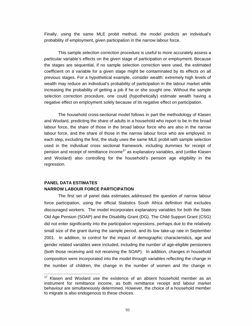
93
Finally, using the same MLE probit method, the model predicts an individual’s probability of employment, given participation in the narrow labour force.
This sample selection correction procedure is useful to more accurately assess a particular variable’s effects on the given stage of participation or employment. Because the stages are sequential, if no sample selection correction were used, the estimated coefficient on a variable for a given stage might be contaminated by its effects on all previous stages. For a hypothetical example, consider wealth: extremely high levels of wealth may reduce an individual’s probability of participation in the labour market while increasing the probability of getting a job if he or she sought one. Without the sample selection correction procedure, one could (hypothetically) estimate wealth having a negative effect on employment solely because of its negative effect on participation.
The household cross-sectional model follows in part the methodology of Klasen and Woolard, predicting the share of adults in a household who report to be in the broad labour force, the share of those in the broad labour force who are also in the narrow labour force, and the share of those in the narrow labour force who are employed. In each step, excluding the first, the study uses the same MLE probit with sample selection used in the individual cross sectional framework, including dummies for receipt of pension and receipt of remittance income37 as explanatory variables, and (unlike Klasen and Woolard) also controlling for the household’s pension age eligibility in the regression. PANEL DATA ESTIMATES NARROW LABOUR FORCE PARTICIPATION
The first set of panel data estimates addressed the question of narrow labour force participation, using the official Statistics South Africa definition that excludes discouraged workers. The model incorporates explanatory variables for both the State Old Age Pension (SOAP) and the Disability Grant (DG). The Child Support Grant (CSG) did not enter significantly into the participation regressions, perhaps due to the relatively small size of the grant during the sample period, and its low take-up rate in September 2001. In addition, to control for the impact of demographic characteristics, age and gender related variables were included, including the number of age-eligible pensioners (both those receiving and not receiving the SOAP). In addition, changes in household composition were incorporated into the model through variables reflecting the change in the number of children, the change in the number of women and the change in
17 Klasen and Woolard use the existence of an absent household member as an instrument for remittance income, as both remittance receipt and labour market behaviour are simultaneously determined. However, the choice of a household member to migrate is also endogenous to these choices.
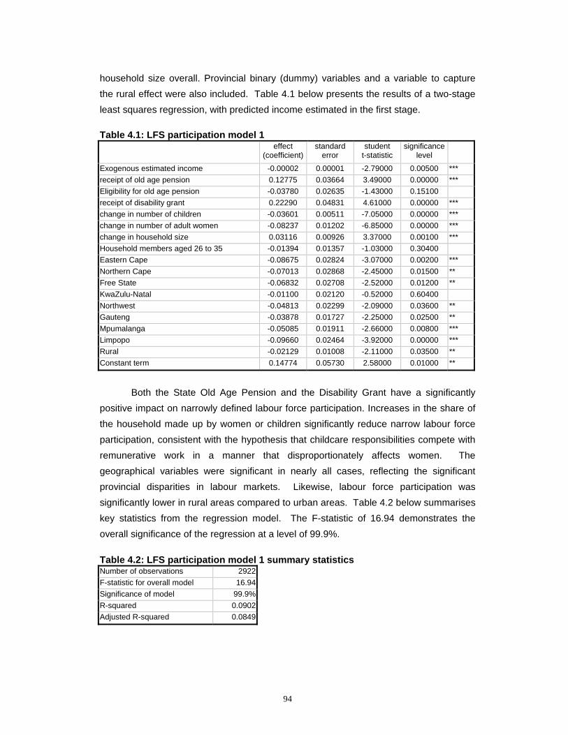
94
household size overall. Provincial binary (dummy) variables and a variable to capture the rural effect were also included. Table 4.1 below presents the results of a two-stage least squares regression, with predicted income estimated in the first stage. Table 4.1: LFS participation model 1
effect (coefficient)
standard error
student t-statistic
significance level
Exogenous estimated income -0.00002 0.00001 -2.79000 0.00500 *** receipt of old age pension 0.12775 0.03664 3.49000 0.00000 *** Eligibility for old age pension -0.03780 0.02635 -1.43000 0.15100 receipt of disability grant 0.22290 0.04831 4.61000 0.00000 *** change in number of children -0.03601 0.00511 -7.05000 0.00000 *** change in number of adult women -0.08237 0.01202 -6.85000 0.00000 *** change in household size 0.03116 0.00926 3.37000 0.00100 *** Household members aged 26 to 35 -0.01394 0.01357 -1.03000 0.30400 Eastern Cape -0.08675 0.02824 -3.07000 0.00200 *** Northern Cape -0.07013 0.02868 -2.45000 0.01500 ** Free State -0.06832 0.02708 -2.52000 0.01200 ** KwaZulu-Natal -0.01100 0.02120 -0.52000 0.60400 Northwest -0.04813 0.02299 -2.09000 0.03600 ** Gauteng -0.03878 0.01727 -2.25000 0.02500 ** Mpumalanga -0.05085 0.01911 -2.66000 0.00800 *** Limpopo -0.09660 0.02464 -3.92000 0.00000 *** Rural -0.02129 0.01008 -2.11000 0.03500 ** Constant term 0.14774 0.05730 2.58000 0.01000 **
Both the State Old Age Pension and the Disability Grant have a significantly
positive impact on narrowly defined labour force participation. Increases in the share of the household made up by women or children significantly reduce narrow labour force participation, consistent with the hypothesis that childcare responsibilities compete with remunerative work in a manner that disproportionately affects women. The geographical variables were significant in nearly all cases, reflecting the significant provincial disparities in labour markets. Likewise, labour force participation was significantly lower in rural areas compared to urban areas. Table 4.2 below summarises key statistics from the regression model. The F-statistic of 16.94 demonstrates the overall significance of the regression at a level of 99.9%. Table 4.2: LFS participation model 1 summary statistics Number of observations 2922F-statistic for overall model 16.94Significance of model 99.9%R-squared 0.0902Adjusted R-squared 0.0849
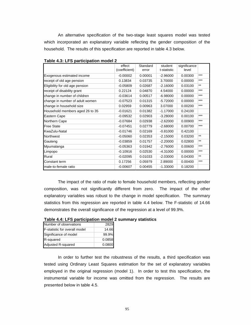
95
An alternative specification of the two-stage least squares model was tested which incorporated an explanatory variable reflecting the gender composition of the household. The results of this specification are reported in table 4.3 below. Table 4.3: LFS participation model 2
effect (coefficient)
Standard error
student t-statistic
significance level
Exogenous estimated income -0.00002 0.00001 -2.96000 0.00300 *** receipt of old age pension 0.13834 0.03735 3.70000 0.00000 *** Eligibility for old age pension -0.05809 0.02687 -2.16000 0.03100 ** receipt of disability grant 0.22124 0.04870 4.54000 0.00000 *** change in number of children -0.03614 0.00517 -6.98000 0.00000 *** change in number of adult women -0.07523 0.01315 -5.72000 0.00000 *** change in household size 0.02959 0.00963 3.07000 0.00200 *** Household members aged 26 to 35 -0.01621 0.01382 -1.17000 0.24100 Eastern Cape -0.09532 0.02903 -3.28000 0.00100 *** Northern Cape -0.07684 0.02938 -2.62000 0.00900 *** Free State -0.07451 0.02779 -2.68000 0.00700 *** KwaZulu-Natal -0.01746 0.02169 -0.81000 0.42100 Northwest -0.05060 0.02353 -2.15000 0.03200 ** Gauteng -0.03859 0.01757 -2.20000 0.02800 ** Mpumalanga -0.05363 0.01942 -2.76000 0.00600 *** Limpopo -0.10916 0.02530 -4.31000 0.00000 *** Rural -0.02095 0.01033 -2.03000 0.04300 ** Constant term 0.17256 0.05979 2.89000 0.00400 *** male-to-female ratio -0.00607 0.00455 -1.33000 0.18200
The impact of the ratio of male to female household members, reflecting gender composition, was not significantly different from zero. The impact of the other explanatory variables was robust to the change in model specification. The summary statistics from this regression are reported in table 4.4 below. The F-statistic of 14.66 demonstrates the overall significance of the regression at a level of 99.9%. Table 4.4: LFS participation model 2 summary statistics Number of observations 2829F-statistic for overall model 14.66Significance of model 99.9%R-squared 0.0858Adjusted R-squared 0.0800
In order to further test the robustness of the results, a third specification was tested using Ordinary Least Squares estimation for the set of explanatory variables employed in the original regression (model 1). In order to test this specification, the instrumental variable for income was omitted from the regression. The results are presented below in table 4.5.
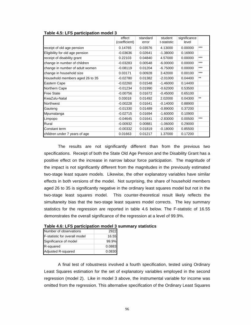
96
Table 4.5: LFS participation model 3 effect
(coefficient)standard
error student
t-statistic significance
level
receipt of old age pension 0.14765 0.03576 4.13000 0.00000 *** Eligibility for old age pension -0.03636 0.02641 -1.38000 0.16900 receipt of disability grant 0.22103 0.04840 4.57000 0.00000 *** change in number of children -0.03283 0.00548 -6.00000 0.00000 *** change in number of adult women -0.08119 0.01204 -6.75000 0.00000 *** change in household size 0.03171 0.00928 3.42000 0.00100 *** Household members aged 26 to 35 -0.02780 0.01382 -2.01000 0.04400 ** Eastern Cape -0.02260 0.01548 -1.46000 0.14400 Northern Cape -0.01234 0.01990 -0.62000 0.53500 Free State -0.00756 0.01672 -0.45000 0.65100 KwaZulu-Natal 0.03018 0.01492 2.02000 0.04300 ** Northwest -0.00228 0.01641 -0.14000 0.88900 Gauteng -0.01330 0.01489 -0.89000 0.37200 Mpumalanga -0.02715 0.01694 -1.60000 0.10900 Limpopo -0.04645 0.01641 -2.83000 0.00500 *** Rural -0.00932 0.00881 -1.06000 0.29000 Constant term -0.00332 0.01819 -0.18000 0.85500 children under 7 years of age 0.01663 0.01217 1.37000 0.17200
The results are not significantly different than from the previous two specifications. Receipt of both the State Old Age Pension and the Disability Grant has a positive effect on the increase in narrow labour force participation. The magnitude of the impact is not significantly different from the magnitudes in the previously estimated two-stage least square models. Likewise, the other explanatory variables have similar effects in both versions of the model. Not surprising, the share of household members aged 26 to 35 is significantly negative in the ordinary least squares model but not in the two-stage least squares model. This counter-theoretical result likely reflects the simultaneity bias that the two-stage least squares model corrects. The key summary statistics for the regression are reported in table 4.6 below. The F-statistic of 16.55 demonstrates the overall significance of the regression at a level of 99.9%. Table 4.6: LFS participation model 3 summary statistics Number of observations 2922F-statistic for overall model 16.55Significance of model 99.9%R-squared 0.0883Adjusted R-squared 0.0830
A final test of robustness involved a fourth specification, tested using Ordinary
Least Squares estimation for the set of explanatory variables employed in the second regression (model 2). Like in model 3 above, the instrumental variable for income was omitted from the regression. This alternative specification of the Ordinary Least Squares
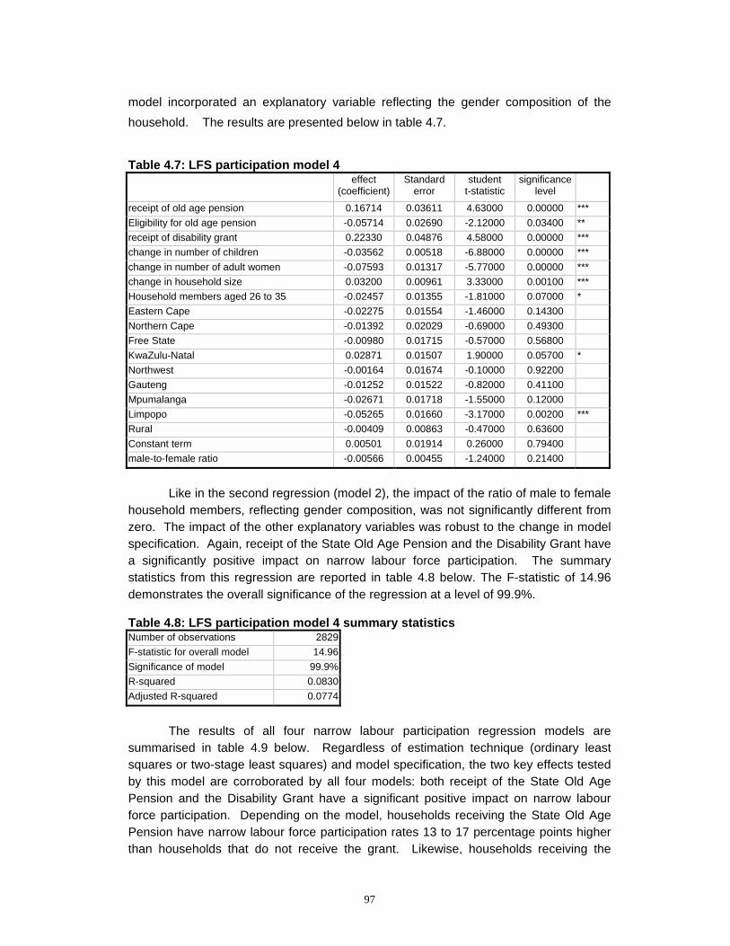
97
model incorporated an explanatory variable reflecting the gender composition of the household. The results are presented below in table 4.7. Table 4.7: LFS participation model 4
effect (coefficient)
Standard error
student t-statistic
significance level
receipt of old age pension 0.16714 0.03611 4.63000 0.00000 *** Eligibility for old age pension -0.05714 0.02690 -2.12000 0.03400 ** receipt of disability grant 0.22330 0.04876 4.58000 0.00000 *** change in number of children -0.03562 0.00518 -6.88000 0.00000 *** change in number of adult women -0.07593 0.01317 -5.77000 0.00000 *** change in household size 0.03200 0.00961 3.33000 0.00100 *** Household members aged 26 to 35 -0.02457 0.01355 -1.81000 0.07000 * Eastern Cape -0.02275 0.01554 -1.46000 0.14300 Northern Cape -0.01392 0.02029 -0.69000 0.49300 Free State -0.00980 0.01715 -0.57000 0.56800 KwaZulu-Natal 0.02871 0.01507 1.90000 0.05700 * Northwest -0.00164 0.01674 -0.10000 0.92200 Gauteng -0.01252 0.01522 -0.82000 0.41100 Mpumalanga -0.02671 0.01718 -1.55000 0.12000 Limpopo -0.05265 0.01660 -3.17000 0.00200 *** Rural -0.00409 0.00863 -0.47000 0.63600 Constant term 0.00501 0.01914 0.26000 0.79400 male-to-female ratio -0.00566 0.00455 -1.24000 0.21400
Like in the second regression (model 2), the impact of the ratio of male to female
household members, reflecting gender composition, was not significantly different from zero. The impact of the other explanatory variables was robust to the change in model specification. Again, receipt of the State Old Age Pension and the Disability Grant have a significantly positive impact on narrow labour force participation. The summary statistics from this regression are reported in table 4.8 below. The F-statistic of 14.96 demonstrates the overall significance of the regression at a level of 99.9%. Table 4.8: LFS participation model 4 summary statistics Number of observations 2829F-statistic for overall model 14.96Significance of model 99.9%R-squared 0.0830Adjusted R-squared 0.0774
The results of all four narrow labour participation regression models are summarised in table 4.9 below. Regardless of estimation technique (ordinary least squares or two-stage least squares) and model specification, the two key effects tested by this model are corroborated by all four models: both receipt of the State Old Age Pension and the Disability Grant have a significant positive impact on narrow labour force participation. Depending on the model, households receiving the State Old Age Pension have narrow labour force participation rates 13 to 17 percentage points higher than households that do not receive the grant. Likewise, households receiving the
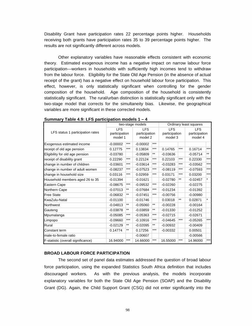
98
Disability Grant have participation rates 22 percentage points higher. Households receiving both grants have participation rates 35 to 39 percentage points higher. The results are not significantly different across models. Other explanatory variables have reasonable effects consistent with economic theory. Estimated exogenous income has a negative impact on narrow labour force participation—workers in households with sufficiently high incomes tend to withdraw from the labour force. Eligibility for the State Old Age Pension (in the absence of actual receipt of the grant) has a negative effect on household labour force participation. This effect, however, is only statistically significant when controlling for the gender composition of the household. Age composition of the household is consistently statistically significant. The rural/urban distinction is statistically significant only with the two-stage model that corrects for the simultaneity bias. Likewise, the geographical variables are more significant in these corrected models. Summary Table 4.9: LFS participation models 1 – 4
two-stage models Ordinary least squares
LFS status 1 participation rates LFS
participation model 1
LFS participation
model 2
LFS participation
model 3
LFS participation
model 4
Exogenous estimated income -0.00002 *** -0.00002 *** receipt of old age pension 0.12775 *** 0.13834 *** 0.14765 *** 0.16714 ***Eligibility for old age pension -0.03780 -0.05809 ** -0.03636 -0.05714 **receipt of disability grant 0.22290 *** 0.22124 *** 0.22103 *** 0.22330 ***change in number of children -0.03601 *** -0.03614 *** -0.03283 *** -0.03562 ***change in number of adult women -0.08237 *** -0.07523 *** -0.08119 *** -0.07593 ***change in household size 0.03116 *** 0.02959 *** 0.03171 *** 0.03200 ***Household members aged 26 to 35 -0.01394 -0.01621 -0.02780 ** -0.02457 * Eastern Cape -0.08675 *** -0.09532 *** -0.02260 -0.02275 Northern Cape -0.07013 ** -0.07684 *** -0.01234 -0.01392 Free State -0.06832 ** -0.07451 *** -0.00756 -0.00980 KwaZulu-Natal -0.01100 -0.01746 0.03018 ** 0.02871 * Northwest -0.04813 ** -0.05060 ** -0.00228 -0.00164 Gauteng -0.03878 ** -0.03859 ** -0.01330 -0.01252 Mpumalanga -0.05085 *** -0.05363 *** -0.02715 -0.02671 Limpopo -0.09660 *** -0.10916 *** -0.04645 *** -0.05265 ***Rural -0.02129 ** -0.02095 ** -0.00932 -0.00409 Constant term 0.14774 ** 0.17256 *** -0.00332 0.00501 male-to-female ratio -0.00607 -0.00566 F-statistic (overall significance) 16.94000 *** 14.66000 *** 16.55000 *** 14.96000 ***
BROAD LABOUR FORCE PARTICIPATION
The second set of panel data estimates addressed the question of broad labour force participation, using the expanded Statistics South Africa definition that includes discouraged workers. As with the previous analysis, the models incorporate explanatory variables for both the State Old Age Pension (SOAP) and the Disability Grant (DG). Again, the Child Support Grant (CSG) did not enter significantly into the
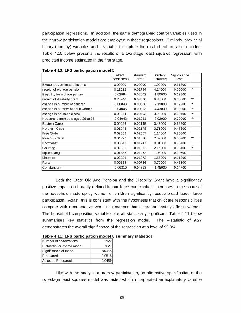
99
participation regressions. In addition, the same demographic control variables used in the narrow participation models are employed in these regressions. Similarly, provincial binary (dummy) variables and a variable to capture the rural effect are also included. Table 4.10 below presents the results of a two-stage least squares regression, with predicted income estimated in the first stage. Table 4.10: LFS participation model 5
effect (coefficient)
standard error
student t-statistic
Significance level
Exogenous estimated income 0.00000 0.00000 1.00000 0.31600 receipt of old age pension 0.11512 0.02784 4.14000 0.00000 *** Eligibility for old age pension -0.02994 0.02002 -1.50000 0.13500 receipt of disability grant 0.25240 0.03670 6.88000 0.00000 *** change in number of children -0.00848 0.00388 -2.19000 0.02900 ** change in number of adult women -0.04046 0.00913 -4.43000 0.00000 *** change in household size 0.02274 0.00703 3.23000 0.00100 *** Household members aged 26 to 35 -0.04043 0.01031 -3.92000 0.00000 *** Eastern Cape 0.00926 0.02145 0.43000 0.66600 Northern Cape 0.01543 0.02178 0.71000 0.47900 Free State 0.02353 0.02057 1.14000 0.25300 KwaZulu-Natal 0.04327 0.01610 2.69000 0.00700 *** Northwest 0.00548 0.01747 0.31000 0.75400 Gauteng 0.02831 0.01312 2.16000 0.03100 ** Mpumalanga 0.01488 0.01452 1.03000 0.30500 Limpopo 0.02926 0.01872 1.56000 0.11800 Rural 0.00535 0.00766 0.70000 0.48500 Constant term -0.06310 0.04353 -1.45000 0.14700
Both the State Old Age Pension and the Disability Grant have a significantly
positive impact on broadly defined labour force participation. Increases in the share of the household made up by women or children significantly reduce broad labour force participation. Again, this is consistent with the hypothesis that childcare responsibilities compete with remunerative work in a manner that disproportionately affects women. The household composition variables are all statistically significant. Table 4.11 below summarises key statistics from the regression model. The F-statistic of 9.27 demonstrates the overall significance of the regression at a level of 99.9%. Table 4.11: LFS participation model 5 summary statistics Number of observations 2922F-statistic for overall model 9.27Significance of model 99.9%R-squared 0.0515Adjusted R-squared 0.0459
Like with the analysis of narrow participation, an alternative specification of the two-stage least squares model was tested which incorporated an explanatory variable
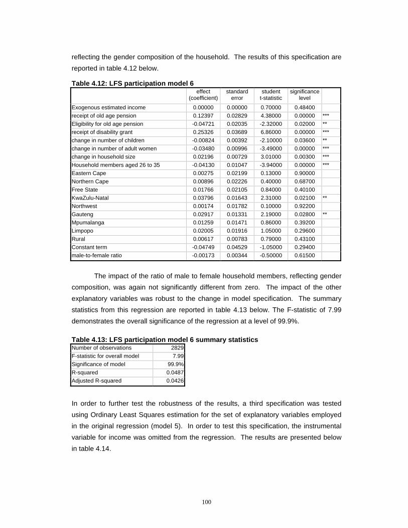
100
reflecting the gender composition of the household. The results of this specification are reported in table 4.12 below. Table 4.12: LFS participation model 6
effect (coefficient)
standard error
student t-statistic
significance level
Exogenous estimated income 0.00000 0.00000 0.70000 0.48400 receipt of old age pension 0.12397 0.02829 4.38000 0.00000 *** Eligibility for old age pension -0.04721 0.02035 -2.32000 0.02000 ** receipt of disability grant 0.25326 0.03689 6.86000 0.00000 *** change in number of children -0.00824 0.00392 -2.10000 0.03600 ** change in number of adult women -0.03480 0.00996 -3.49000 0.00000 *** change in household size 0.02196 0.00729 3.01000 0.00300 *** Household members aged 26 to 35 -0.04130 0.01047 -3.94000 0.00000 *** Eastern Cape 0.00275 0.02199 0.13000 0.90000 Northern Cape 0.00896 0.02226 0.40000 0.68700 Free State 0.01766 0.02105 0.84000 0.40100 KwaZulu-Natal 0.03796 0.01643 2.31000 0.02100 ** Northwest 0.00174 0.01782 0.10000 0.92200 Gauteng 0.02917 0.01331 2.19000 0.02800 ** Mpumalanga 0.01259 0.01471 0.86000 0.39200 Limpopo 0.02005 0.01916 1.05000 0.29600 Rural 0.00617 0.00783 0.79000 0.43100 Constant term -0.04749 0.04529 -1.05000 0.29400 male-to-female ratio -0.00173 0.00344 -0.50000 0.61500
The impact of the ratio of male to female household members, reflecting gender composition, was again not significantly different from zero. The impact of the other explanatory variables was robust to the change in model specification. The summary statistics from this regression are reported in table 4.13 below. The F-statistic of 7.99 demonstrates the overall significance of the regression at a level of 99.9%. Table 4.13: LFS participation model 6 summary statistics Number of observations 2829F-statistic for overall model 7.99Significance of model 99.9%R-squared 0.0487Adjusted R-squared 0.0426
In order to further test the robustness of the results, a third specification was tested using Ordinary Least Squares estimation for the set of explanatory variables employed in the original regression (model 5). In order to test this specification, the instrumental variable for income was omitted from the regression. The results are presented below in table 4.14.
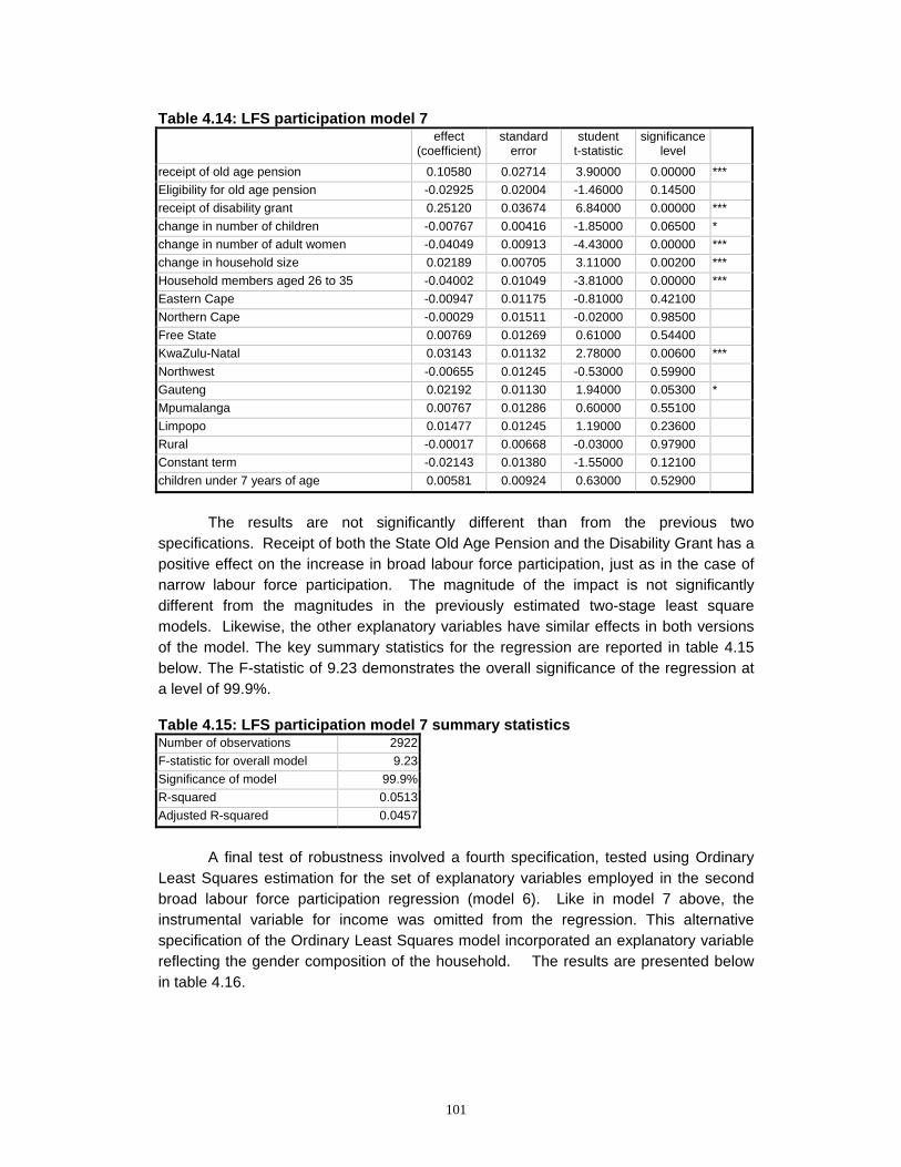
101
Table 4.14: LFS participation model 7 effect
(coefficient)standard
error student
t-statistic significance
level
receipt of old age pension 0.10580 0.02714 3.90000 0.00000 *** Eligibility for old age pension -0.02925 0.02004 -1.46000 0.14500 receipt of disability grant 0.25120 0.03674 6.84000 0.00000 *** change in number of children -0.00767 0.00416 -1.85000 0.06500 * change in number of adult women -0.04049 0.00913 -4.43000 0.00000 *** change in household size 0.02189 0.00705 3.11000 0.00200 *** Household members aged 26 to 35 -0.04002 0.01049 -3.81000 0.00000 *** Eastern Cape -0.00947 0.01175 -0.81000 0.42100 Northern Cape -0.00029 0.01511 -0.02000 0.98500 Free State 0.00769 0.01269 0.61000 0.54400 KwaZulu-Natal 0.03143 0.01132 2.78000 0.00600 *** Northwest -0.00655 0.01245 -0.53000 0.59900 Gauteng 0.02192 0.01130 1.94000 0.05300 * Mpumalanga 0.00767 0.01286 0.60000 0.55100 Limpopo 0.01477 0.01245 1.19000 0.23600 Rural -0.00017 0.00668 -0.03000 0.97900 Constant term -0.02143 0.01380 -1.55000 0.12100 children under 7 years of age 0.00581 0.00924 0.63000 0.52900
The results are not significantly different than from the previous two
specifications. Receipt of both the State Old Age Pension and the Disability Grant has a positive effect on the increase in broad labour force participation, just as in the case of narrow labour force participation. The magnitude of the impact is not significantly different from the magnitudes in the previously estimated two-stage least square models. Likewise, the other explanatory variables have similar effects in both versions of the model. The key summary statistics for the regression are reported in table 4.15 below. The F-statistic of 9.23 demonstrates the overall significance of the regression at a level of 99.9%. Table 4.15: LFS participation model 7 summary statistics Number of observations 2922F-statistic for overall model 9.23Significance of model 99.9%R-squared 0.0513Adjusted R-squared 0.0457
A final test of robustness involved a fourth specification, tested using Ordinary
Least Squares estimation for the set of explanatory variables employed in the second broad labour force participation regression (model 6). Like in model 7 above, the instrumental variable for income was omitted from the regression. This alternative specification of the Ordinary Least Squares model incorporated an explanatory variable reflecting the gender composition of the household. The results are presented below in table 4.16.
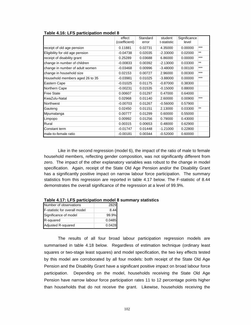
102
Table 4.16: LFS participation model 8 effect
(coefficient)Standard
error student
t-statistic Significance
level
receipt of old age pension 0.11881 0.02731 4.35000 0.00000 *** Eligibility for old age pension -0.04738 0.02035 -2.33000 0.02000 ** receipt of disability grant 0.25289 0.03688 6.86000 0.00000 *** change in number of children -0.00833 0.00392 -2.13000 0.03300 ** change in number of adult women -0.03468 0.00996 -3.48000 0.00100 *** change in household size 0.02153 0.00727 2.96000 0.00300 *** Household members aged 26 to 35 -0.03981 0.01025 -3.88000 0.00000 *** Eastern Cape -0.01025 0.01175 -0.87000 0.38300 Northern Cape -0.00231 0.01535 -0.15000 0.88000 Free State 0.00607 0.01297 0.47000 0.64000 KwaZulu-Natal 0.02968 0.01140 2.60000 0.00900 *** Northwest -0.00703 0.01267 -0.56000 0.57900 Gauteng 0.02450 0.01151 2.13000 0.03300 ** Mpumalanga 0.00777 0.01299 0.60000 0.55000 Limpopo 0.00992 0.01256 0.79000 0.43000 Rural 0.00315 0.00653 0.48000 0.62900 Constant term -0.01747 0.01448 -1.21000 0.22800 male-to-female ratio -0.00181 0.00344 -0.52000 0.60000
Like in the second regression (model 6), the impact of the ratio of male to female household members, reflecting gender composition, was not significantly different from zero. The impact of the other explanatory variables was robust to the change in model specification. Again, receipt of the State Old Age Pension and/or the Disability Grant has a significantly positive impact on narrow labour force participation. The summary statistics from this regression are reported in table 4.17 below. The F-statistic of 8.44 demonstrates the overall significance of the regression at a level of 99.9%. Table 4.17: LFS participation model 8 summary statistics Number of observations 2829F-statistic for overall model 8.44Significance of model 99.9%R-squared 0.0485Adjusted R-squared 0.0428
The results of all four broad labour participation regression models are
summarised in table 4.18 below. Regardless of estimation technique (ordinary least squares or two-stage least squares) and model specification, the two key effects tested by this model are corroborated by all four models: both receipt of the State Old Age Pension and the Disability Grant have a significant positive impact on broad labour force participation. Depending on the model, households receiving the State Old Age Pension have narrow labour force participation rates 11 to 12 percentage points higher than households that do not receive the grant. Likewise, households receiving the
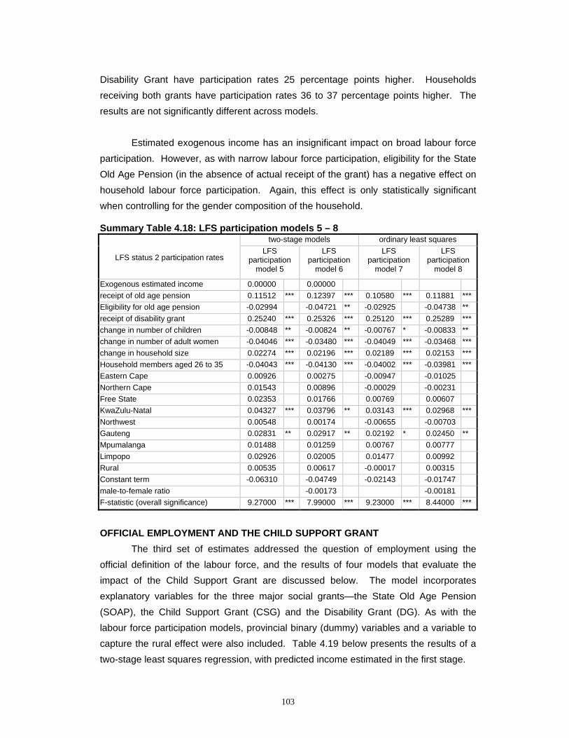
103
Disability Grant have participation rates 25 percentage points higher. Households receiving both grants have participation rates 36 to 37 percentage points higher. The results are not significantly different across models. Estimated exogenous income has an insignificant impact on broad labour force participation. However, as with narrow labour force participation, eligibility for the State Old Age Pension (in the absence of actual receipt of the grant) has a negative effect on household labour force participation. Again, this effect is only statistically significant when controlling for the gender composition of the household. Summary Table 4.18: LFS participation models 5 – 8
two-stage models ordinary least squares
LFS status 2 participation rates LFS
participation model 5
LFS participation
model 6
LFS participation
model 7
LFS participation
model 8
Exogenous estimated income 0.00000 0.00000 receipt of old age pension 0.11512 *** 0.12397 *** 0.10580 *** 0.11881 *** Eligibility for old age pension -0.02994 -0.04721 ** -0.02925 -0.04738 ** receipt of disability grant 0.25240 *** 0.25326 *** 0.25120 *** 0.25289 *** change in number of children -0.00848 ** -0.00824 ** -0.00767 * -0.00833 ** change in number of adult women -0.04046 *** -0.03480 *** -0.04049 *** -0.03468 *** change in household size 0.02274 *** 0.02196 *** 0.02189 *** 0.02153 *** Household members aged 26 to 35 -0.04043 *** -0.04130 *** -0.04002 *** -0.03981 *** Eastern Cape 0.00926 0.00275 -0.00947 -0.01025 Northern Cape 0.01543 0.00896 -0.00029 -0.00231 Free State 0.02353 0.01766 0.00769 0.00607 KwaZulu-Natal 0.04327 *** 0.03796 ** 0.03143 *** 0.02968 *** Northwest 0.00548 0.00174 -0.00655 -0.00703 Gauteng 0.02831 ** 0.02917 ** 0.02192 * 0.02450 ** Mpumalanga 0.01488 0.01259 0.00767 0.00777 Limpopo 0.02926 0.02005 0.01477 0.00992 Rural 0.00535 0.00617 -0.00017 0.00315 Constant term -0.06310 -0.04749 -0.02143 -0.01747 male-to-female ratio -0.00173 -0.00181 F-statistic (overall significance) 9.27000 *** 7.99000 *** 9.23000 *** 8.44000 ***
OFFICIAL EMPLOYMENT AND THE CHILD SUPPORT GRANT
The third set of estimates addressed the question of employment using the official definition of the labour force, and the results of four models that evaluate the impact of the Child Support Grant are discussed below. The model incorporates explanatory variables for the three major social grants—the State Old Age Pension (SOAP), the Child Support Grant (CSG) and the Disability Grant (DG). As with the labour force participation models, provincial binary (dummy) variables and a variable to capture the rural effect were also included. Table 4.19 below presents the results of a two-stage least squares regression, with predicted income estimated in the first stage.
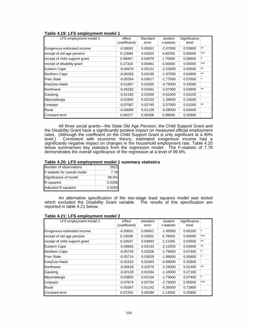
104
Table 4.19: LFS employment model 1 LFS employment model 1 effect
(coefficient)Standard
error student
t-statistic Significance
level
Exogenous estimated income -0.00001 0.00001 -2.07000 0.03900 ** receipt of old age pension 0.12684 0.02632 4.82000 0.00000 *** receipt of child support grant 0.08467 0.04979 1.70000 0.08900 * receipt of disability grant 0.27316 0.05461 5.00000 0.00000 *** Eastern Cape -0.06978 0.03131 -2.23000 0.02600 ** Northern Cape -0.06283 0.03195 -1.97000 0.04900 ** Free State -0.05354 0.03017 -1.77000 0.07600 * KwaZulu-Natal -0.01857 0.02355 -0.79000 0.43000 Northwest -0.05292 0.02561 -2.07000 0.03900 ** Gauteng -0.01182 0.01935 -0.61000 0.54100 Mpumalanga -0.02992 0.02152 -1.39000 0.16500 Limpopo -0.07067 0.02745 -2.57000 0.01000 ** Rural -0.00095 0.01139 -0.08000 0.93400 Constant term 0.06217 0.06358 0.98000 0.32800
All three social grants—the State Old Age Pension, the Child Support Grant and
the Disability Grant have a significantly positive impact on measured official employment rates. (Although the coefficient on the Child Support Grant is only significant at a 90% level.) Consistent with economic theory, estimated exogenous income had a significantly negative impact on changes in the household employment rate. Table 4.20 below summarises key statistics from the regression model. The F-statistic of 7.78 demonstrates the overall significance of the regression at a level of 99.9%. Table 4.20: LFS employment model 1 summary statistics Number of observations 2922F-statistic for overall model 7.78Significance of model 99.9%R-squared 0.0336Adjusted R-squared 0.0293
An alternative specification of the two-stage least squares model was tested
which excluded the Disability Grant variable. The results of this specification are reported in table 4.21 below. Table 4.21: LFS employment model 2
LFS employment model 2 Effect (coefficient)
standard error
student t-statistic
significance level
Exogenous estimated income -0.00001 0.00001 -1.95000 0.05200 * receipt of old age pension 0.15039 0.02601 5.78000 0.00000 *** receipt of child support grant 0.10507 0.04983 2.11000 0.03500 ** Eastern Cape -0.06662 0.03143 -2.12000 0.03400 ** Northern Cape -0.05725 0.03206 -1.79000 0.07400 * Free State -0.05714 0.03029 -1.89000 0.05900 * KwaZulu-Natal -0.02310 0.02363 -0.98000 0.32800 Northwest -0.05818 0.02570 -2.26000 0.02400 ** Gauteng -0.02128 0.01934 -1.10000 0.27100 Mpumalanga -0.03853 0.02154 -1.79000 0.07400 * Limpopo -0.07674 0.02754 -2.79000 0.00500 *** Rural -0.00397 0.01142 -0.35000 0.72800 Constant term 0.07254 0.06380 1.14000 0.25600
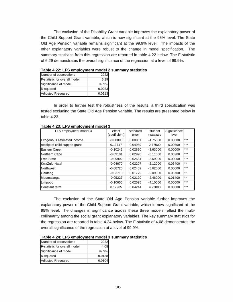
105
The exclusion of the Disability Grant variable improves the explanatory power of the Child Support Grant variable, which is now significant at the 95% level. The State Old Age Pension variable remains significant at the 99.9% level. The impacts of the other explanatory variables were robust to the change in model specification. The summary statistics from this regression are reported in table 4.22 below. The F-statistic of 6.29 demonstrates the overall significance of the regression at a level of 99.9%. Table 4.22: LFS employment model 2 summary statistics Number of observations 2922F-statistic for overall model 6.29Significance of model 99.9%R-squared 0.0253Adjusted R-squared 0.0213
In order to further test the robustness of the results, a third specification was
tested excluding the State Old Age Pension variable. The results are presented below in table 4.23. Table 4.23: LFS employment model 3
LFS employment model 3 effect (coefficient)
standard error
student t-statistic
Significance level
Exogenous estimated income -0.00003 0.00001 -4.75000 0.00000 *** receipt of child support grant 0.13747 0.04959 2.77000 0.00600 *** Eastern Cape -0.10242 0.02820 -3.63000 0.00000 *** Northern Cape -0.09101 0.02928 -3.11000 0.00200 *** Free State -0.09902 0.02684 -3.69000 0.00000 *** KwaZulu-Natal -0.04670 0.02207 -2.12000 0.03400 ** Northwest -0.08726 0.02409 -3.62000 0.00000 *** Gauteng -0.03713 0.01779 -2.09000 0.03700 ** Mpumalanga -0.05227 0.02120 -2.46000 0.01400 ** Limpopo -0.10650 0.02595 -4.10000 0.00000 *** Constant term 0.17905 0.04244 4.22000 0.00000 ***
The exclusion of the State Old Age Pension variable further improves the explanatory power of the Child Support Grant variable, which is now significant at the 99% level. The changes in significance across these three models reflect the multi-collinearity among the social grant explanatory variables. The key summary statistics for the regression are reported in table 4.24 below. The F-statistic of 4.08 demonstrates the overall significance of the regression at a level of 99.9%. Table 4.24: LFS employment model 3 summary statistics Number of observations 2922F-statistic for overall model 4.08Significance of model 99.9%R-squared 0.0138Adjusted R-squared 0.0104
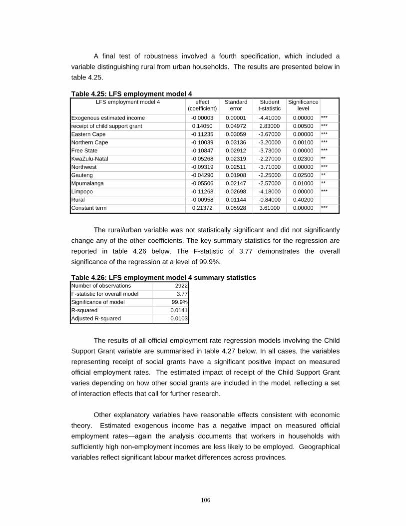
106
A final test of robustness involved a fourth specification, which included a variable distinguishing rural from urban households. The results are presented below in table 4.25. Table 4.25: LFS employment model 4
LFS employment model 4 effect (coefficient)
Standard error
Student t-statistic
Significance level
Exogenous estimated income -0.00003 0.00001 -4.41000 0.00000 *** receipt of child support grant 0.14050 0.04972 2.83000 0.00500 *** Eastern Cape -0.11235 0.03059 -3.67000 0.00000 *** Northern Cape -0.10039 0.03136 -3.20000 0.00100 *** Free State -0.10847 0.02912 -3.73000 0.00000 *** KwaZulu-Natal -0.05268 0.02319 -2.27000 0.02300 ** Northwest -0.09319 0.02511 -3.71000 0.00000 *** Gauteng -0.04290 0.01908 -2.25000 0.02500 ** Mpumalanga -0.05506 0.02147 -2.57000 0.01000 ** Limpopo -0.11268 0.02698 -4.18000 0.00000 *** Rural -0.00958 0.01144 -0.84000 0.40200 Constant term 0.21372 0.05928 3.61000 0.00000 ***
The rural/urban variable was not statistically significant and did not significantly
change any of the other coefficients. The key summary statistics for the regression are reported in table 4.26 below. The F-statistic of 3.77 demonstrates the overall significance of the regression at a level of 99.9%. Table 4.26: LFS employment model 4 summary statistics Number of observations 2922F-statistic for overall model 3.77Significance of model 99.9%R-squared 0.0141Adjusted R-squared 0.0103
The results of all official employment rate regression models involving the Child
Support Grant variable are summarised in table 4.27 below. In all cases, the variables representing receipt of social grants have a significant positive impact on measured official employment rates. The estimated impact of receipt of the Child Support Grant varies depending on how other social grants are included in the model, reflecting a set of interaction effects that call for further research.
Other explanatory variables have reasonable effects consistent with economic theory. Estimated exogenous income has a negative impact on measured official employment rates—again the analysis documents that workers in households with sufficiently high non-employment incomes are less likely to be employed. Geographical variables reflect significant labour market differences across provinces.
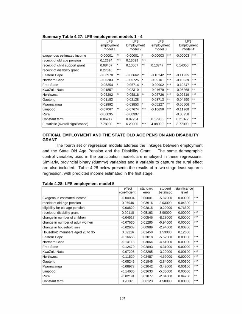
107
Summary Table 4.27: LFS employment models 1 - 4
LFS employment
model 1
LFS Employment
model 2
LFS employment
model 3
LFS Employment
model 4
exogenous estimated income -0.00001 ** -0.00001 * -0.00003 *** -0.00003 *** receipt of old age pension 0.12684 *** 0.15039 *** receipt of child support grant 0.08467 * 0.10507 ** 0.13747 *** 0.14050 *** receipt of disability grant 0.27316 *** Eastern Cape -0.06978 ** -0.06662 ** -0.10242 *** -0.11235 *** Northern Cape -0.06283 ** -0.05725 * -0.09101 *** -0.10039 *** Free State -0.05354 * -0.05714 * -0.09902 *** -0.10847 *** KwaZulu-Natal -0.01857 -0.02310 -0.04670 ** -0.05268 ** Northwest -0.05292 ** -0.05818 ** -0.08726 *** -0.09319 *** Gauteng -0.01182 -0.02128 -0.03713 ** -0.04290 ** Mpumalanga -0.02992 -0.03853 * -0.05227 ** -0.05506 ** Limpopo -0.07067 ** -0.07674 *** -0.10650 *** -0.11268 *** Rural -0.00095 -0.00397 -0.00958 Constant term 0.06217 0.07254 0.17905 *** 0.21372 *** F-statistic (overall significance) 7.78000 *** 6.29000 *** 4.08000 *** 3.77000 ***
OFFICIAL EMPLOYMENT AND THE STATE OLD AGE PENSION AND DISABILITY GRANT
The fourth set of regression models address the linkages between employment and the State Old Age Pension and the Disability Grant. The same demographic control variables used in the participation models are employed in these regressions. Similarly, provincial binary (dummy) variables and a variable to capture the rural effect are also included. Table 4.28 below presents the results of a two-stage least squares regression, with predicted income estimated in the first stage.
Table 4.28: LFS employment model 5
effect (coefficient)
standard error
student t-statistic
significance level
Exogenous estimated income -0.00004 0.00001 -5.87000 0.00000 *** receipt of old age pension 0.07946 0.03916 2.03000 0.04300 ** eligibility for old age pension -0.00829 0.02815 -0.29000 0.76800 receipt of disability grant 0.20110 0.05163 3.90000 0.00000 *** change in number of children -0.04517 0.00546 -8.28000 0.00000 *** change in number of adult women -0.07630 0.01285 -5.94000 0.00000 *** change in household size -0.02903 0.00989 -2.94000 0.00300 *** Household members aged 26 to 35 0.02216 0.01450 1.53000 0.12600 Eastern Cape -0.16665 0.03018 -5.52000 0.00000 *** Northern Cape -0.14113 0.03064 -4.61000 0.00000 *** Free State -0.12470 0.02893 -4.31000 0.00000 *** KwaZulu-Natal -0.07296 0.02265 -3.22000 0.00100 *** Northwest -0.11520 0.02457 -4.69000 0.00000 *** Gauteng -0.05245 0.01845 -2.84000 0.00500 *** Mpumalanga -0.06978 0.02042 -3.42000 0.00100 *** Limpopo -0.14086 0.02633 -5.35000 0.00000 *** Rural -0.02191 0.01077 -2.04000 0.04200 ** Constant term 0.28061 0.06123 4.58000 0.00000 ***
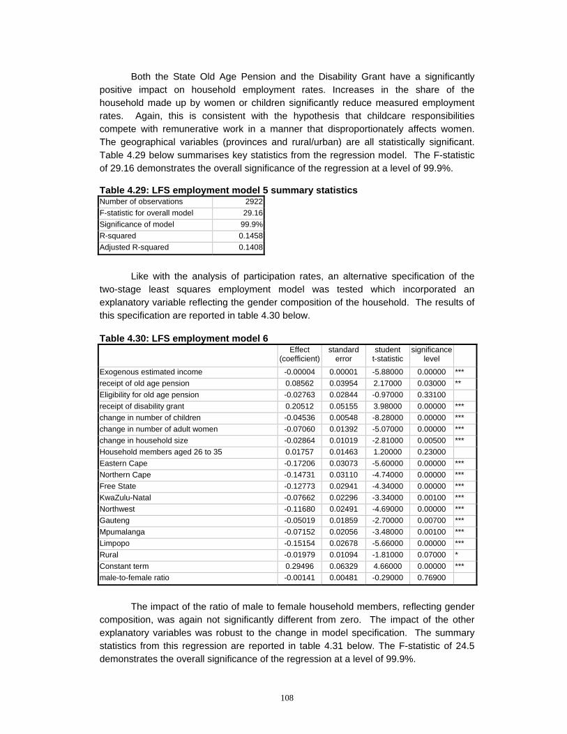
108
Both the State Old Age Pension and the Disability Grant have a significantly positive impact on household employment rates. Increases in the share of the household made up by women or children significantly reduce measured employment rates. Again, this is consistent with the hypothesis that childcare responsibilities compete with remunerative work in a manner that disproportionately affects women. The geographical variables (provinces and rural/urban) are all statistically significant. Table 4.29 below summarises key statistics from the regression model. The F-statistic of 29.16 demonstrates the overall significance of the regression at a level of 99.9%. Table 4.29: LFS employment model 5 summary statistics Number of observations 2922F-statistic for overall model 29.16Significance of model 99.9%R-squared 0.1458Adjusted R-squared 0.1408
Like with the analysis of participation rates, an alternative specification of the
two-stage least squares employment model was tested which incorporated an explanatory variable reflecting the gender composition of the household. The results of this specification are reported in table 4.30 below. Table 4.30: LFS employment model 6
Effect (coefficient)
standard error
student t-statistic
significance level
Exogenous estimated income -0.00004 0.00001 -5.88000 0.00000 *** receipt of old age pension 0.08562 0.03954 2.17000 0.03000 ** Eligibility for old age pension -0.02763 0.02844 -0.97000 0.33100 receipt of disability grant 0.20512 0.05155 3.98000 0.00000 *** change in number of children -0.04536 0.00548 -8.28000 0.00000 *** change in number of adult women -0.07060 0.01392 -5.07000 0.00000 *** change in household size -0.02864 0.01019 -2.81000 0.00500 *** Household members aged 26 to 35 0.01757 0.01463 1.20000 0.23000 Eastern Cape -0.17206 0.03073 -5.60000 0.00000 *** Northern Cape -0.14731 0.03110 -4.74000 0.00000 *** Free State -0.12773 0.02941 -4.34000 0.00000 *** KwaZulu-Natal -0.07662 0.02296 -3.34000 0.00100 *** Northwest -0.11680 0.02491 -4.69000 0.00000 *** Gauteng -0.05019 0.01859 -2.70000 0.00700 *** Mpumalanga -0.07152 0.02056 -3.48000 0.00100 *** Limpopo -0.15154 0.02678 -5.66000 0.00000 *** Rural -0.01979 0.01094 -1.81000 0.07000 * Constant term 0.29496 0.06329 4.66000 0.00000 *** male-to-female ratio -0.00141 0.00481 -0.29000 0.76900
The impact of the ratio of male to female household members, reflecting gender
composition, was again not significantly different from zero. The impact of the other explanatory variables was robust to the change in model specification. The summary statistics from this regression are reported in table 4.31 below. The F-statistic of 24.5 demonstrates the overall significance of the regression at a level of 99.9%.
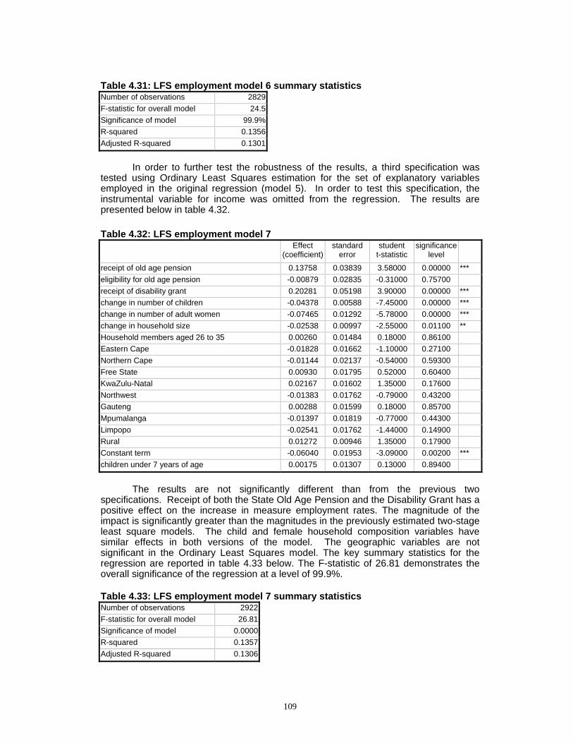
109
Table 4.31: LFS employment model 6 summary statistics Number of observations 2829F-statistic for overall model 24.5Significance of model 99.9%R-squared 0.1356Adjusted R-squared 0.1301
In order to further test the robustness of the results, a third specification was tested using Ordinary Least Squares estimation for the set of explanatory variables employed in the original regression (model 5). In order to test this specification, the instrumental variable for income was omitted from the regression. The results are presented below in table 4.32. Table 4.32: LFS employment model 7
Effect (coefficient)
standard error
student t-statistic
significance level
receipt of old age pension 0.13758 0.03839 3.58000 0.00000 *** eligibility for old age pension -0.00879 0.02835 -0.31000 0.75700 receipt of disability grant 0.20281 0.05198 3.90000 0.00000 *** change in number of children -0.04378 0.00588 -7.45000 0.00000 *** change in number of adult women -0.07465 0.01292 -5.78000 0.00000 *** change in household size -0.02538 0.00997 -2.55000 0.01100 ** Household members aged 26 to 35 0.00260 0.01484 0.18000 0.86100 Eastern Cape -0.01828 0.01662 -1.10000 0.27100 Northern Cape -0.01144 0.02137 -0.54000 0.59300 Free State 0.00930 0.01795 0.52000 0.60400 KwaZulu-Natal 0.02167 0.01602 1.35000 0.17600 Northwest -0.01383 0.01762 -0.79000 0.43200 Gauteng 0.00288 0.01599 0.18000 0.85700 Mpumalanga -0.01397 0.01819 -0.77000 0.44300 Limpopo -0.02541 0.01762 -1.44000 0.14900 Rural 0.01272 0.00946 1.35000 0.17900 Constant term -0.06040 0.01953 -3.09000 0.00200 *** children under 7 years of age 0.00175 0.01307 0.13000 0.89400
The results are not significantly different than from the previous two
specifications. Receipt of both the State Old Age Pension and the Disability Grant has a positive effect on the increase in measure employment rates. The magnitude of the impact is significantly greater than the magnitudes in the previously estimated two-stage least square models. The child and female household composition variables have similar effects in both versions of the model. The geographic variables are not significant in the Ordinary Least Squares model. The key summary statistics for the regression are reported in table 4.33 below. The F-statistic of 26.81 demonstrates the overall significance of the regression at a level of 99.9%. Table 4.33: LFS employment model 7 summary statistics Number of observations 2922F-statistic for overall model 26.81Significance of model 0.0000R-squared 0.1357Adjusted R-squared 0.1306
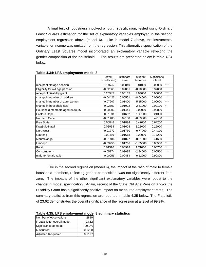
110
A final test of robustness involved a fourth specification, tested using Ordinary Least Squares estimation for the set of explanatory variables employed in the second employment regression above (model 6). Like in model 7 above, the instrumental variable for income was omitted from the regression. This alternative specification of the Ordinary Least Squares model incorporated an explanatory variable reflecting the gender composition of the household. The results are presented below is table 4.34 below.
Table 4.34: LFS employment model 8
effect (coefficient)
standard error
student t-statistic
Significance level
receipt of old age pension 0.14625 0.03840 3.81000 0.00000 *** Eligibility for old age pension -0.02563 0.02861 -0.90000 0.37000 receipt of disability grant 0.20945 0.05185 4.04000 0.00000 *** change in number of children -0.04426 0.00551 -8.04000 0.00000 *** change in number of adult women -0.07207 0.01400 -5.15000 0.00000 *** change in household size -0.02357 0.01022 -2.31000 0.02100 ** Household members aged 26 to 35 -0.00003 0.01441 0.00000 0.99800 Eastern Cape -0.01931 0.01652 -1.17000 0.24300 Northern Cape -0.01485 0.02158 -0.69000 0.49100 Free State 0.00848 0.01824 0.47000 0.64200 KwaZulu-Natal 0.02058 0.01603 1.28000 0.19900 Northwest -0.01373 0.01780 -0.77000 0.44100 Gauteng 0.00469 0.01618 0.29000 0.77200 Mpumalanga -0.01486 0.01827 -0.81000 0.41600 Limpopo -0.03258 0.01766 -1.85000 0.06500 * Rural 0.01570 0.00918 1.71000 0.08700 * Constant term -0.05774 0.02035 -2.84000 0.00500 *** male-to-female ratio -0.00056 0.00484 -0.12000 0.90800
Like in the second regression (model 6), the impact of the ratio of male to female
household members, reflecting gender composition, was not significantly different from zero. The impacts of the other significant explanatory variables were robust to the change in model specification. Again, receipt of the State Old Age Pension and/or the Disability Grant has a significantly positive impact on measured employment rates. The summary statistics from this regression are reported in table 4.35 below. The F-statistic of 23.62 demonstrates the overall significance of the regression at a level of 99.9%. Table 4.35: LFS employment model 8 summary statistics Number of observations 2829F-statistic for overall model 23.62Significance of model 99.9%R-squared 0.1250Adjusted R-squared 0.1197
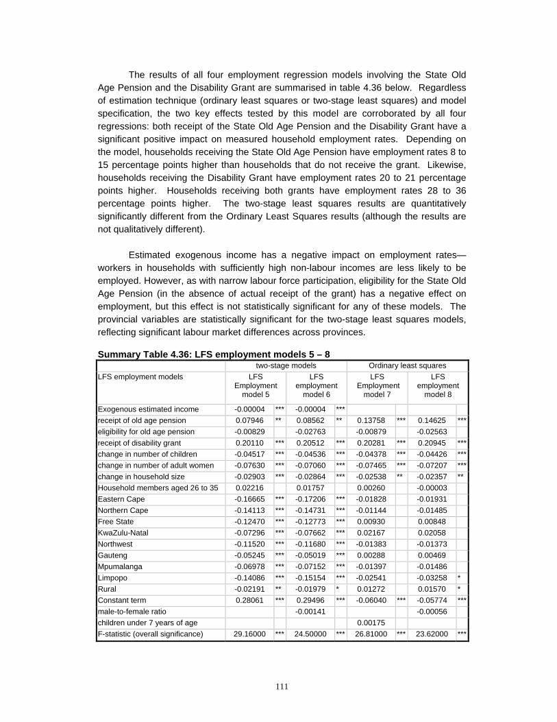
111
The results of all four employment regression models involving the State Old Age Pension and the Disability Grant are summarised in table 4.36 below. Regardless of estimation technique (ordinary least squares or two-stage least squares) and model specification, the two key effects tested by this model are corroborated by all four regressions: both receipt of the State Old Age Pension and the Disability Grant have a significant positive impact on measured household employment rates. Depending on the model, households receiving the State Old Age Pension have employment rates 8 to 15 percentage points higher than households that do not receive the grant. Likewise, households receiving the Disability Grant have employment rates 20 to 21 percentage points higher. Households receiving both grants have employment rates 28 to 36 percentage points higher. The two-stage least squares results are quantitatively significantly different from the Ordinary Least Squares results (although the results are not qualitatively different). Estimated exogenous income has a negative impact on employment rates—workers in households with sufficiently high non-labour incomes are less likely to be employed. However, as with narrow labour force participation, eligibility for the State Old Age Pension (in the absence of actual receipt of the grant) has a negative effect on employment, but this effect is not statistically significant for any of these models. The provincial variables are statistically significant for the two-stage least squares models, reflecting significant labour market differences across provinces. Summary Table 4.36: LFS employment models 5 – 8
two-stage models Ordinary least squares LFS employment models LFS
Employment model 5
LFS employment
model 6
LFS Employment
model 7
LFS employment
model 8
Exogenous estimated income -0.00004 *** -0.00004 *** receipt of old age pension 0.07946 ** 0.08562 ** 0.13758 *** 0.14625 ***eligibility for old age pension -0.00829 -0.02763 -0.00879 -0.02563 receipt of disability grant 0.20110 *** 0.20512 *** 0.20281 *** 0.20945 ***change in number of children -0.04517 *** -0.04536 *** -0.04378 *** -0.04426 ***change in number of adult women -0.07630 *** -0.07060 *** -0.07465 *** -0.07207 ***change in household size -0.02903 *** -0.02864 *** -0.02538 ** -0.02357 **Household members aged 26 to 35 0.02216 0.01757 0.00260 -0.00003 Eastern Cape -0.16665 *** -0.17206 *** -0.01828 -0.01931 Northern Cape -0.14113 *** -0.14731 *** -0.01144 -0.01485 Free State -0.12470 *** -0.12773 *** 0.00930 0.00848 KwaZulu-Natal -0.07296 *** -0.07662 *** 0.02167 0.02058 Northwest -0.11520 *** -0.11680 *** -0.01383 -0.01373 Gauteng -0.05245 *** -0.05019 *** 0.00288 0.00469 Mpumalanga -0.06978 *** -0.07152 *** -0.01397 -0.01486 Limpopo -0.14086 *** -0.15154 *** -0.02541 -0.03258 * Rural -0.02191 ** -0.01979 * 0.01272 0.01570 * Constant term 0.28061 *** 0.29496 *** -0.06040 *** -0.05774 ***male-to-female ratio -0.00141 -0.00056 children under 7 years of age 0.00175 F-statistic (overall significance) 29.16000 *** 24.50000 *** 26.81000 *** 23.62000 ***
112
CROSS-SECTION ESTIMATES The individual labour force participation and employment regressions are
reported in the appendix below. In general, because of sample selection problems and data issues, the results are not robust and most of the social grant variables are not statistically significant. Following the example of Bhorat and Leibbrandt, the econometric analysis estimates separate regressions for males and females broken down into rural and urban sub-samples. The appendix reports both employment and labour force participation regressions, including the sample selection equations in each case.
With respect to labour force participation rates, the effects of the State Old Age
Pension and the Disability Grant are statistically significantly positive for rural females. However, for rural males and urban males and females, all the social grants have effects that are not statistically different from zero. Other economically important variables have fragile relationships to labour force participation, or yield theoretically inconsistent signs.
The results from the employment equations yield somewhat more significant
results. For both rural males and females, the effects of the State Old Age Pension and the Disability Grant are statistically significantly positive. Workers in households receiving either a State Old Age Pension or a Disability Grant are about ten percent more likely to be employed. Workers in households receiving both grants are approximately twenty percent more likely to be employed. However, the effect of the State Old Age Pension for urban males is significantly negative by the same magnitude. The differential effects for urban and rural workers is a persistent theme in the literature on social security’s impact on labour markets. The results identified by the cross-sectional analysis may be spurious because the sample selection methodology is relatively weak in its capacity to control for unobserved heterogeneity in the sample.
Overall, the cross-sectional analysis provides some weak evidence that social
grants have positive effects on both labour market participation and employment. However, the results are not unambiguous and certainly not conclusive. However, they tend to corroborate the stronger results identified by the panel analysis, supporting the findings that social grants have positive labour market effects. 4.4) LABOUR DEMAND
This section builds on the household impact study as well as the evidence from the previous section in order to identify specific transmission mechanisms between social security programmes and worker productivity effects. Social assistance that increases labour productivity has the potential to increase the demand by employers for workers, which is generally measured as the marginal productivity of labour. Directly, social grants support the accumulation of human capital by a worker, and it supports the worker’s productivity-bolstering consumption. Better nutrition, health care, housing and transportation can all support the increased productivity of the worker. Indirectly, social assistance supports higher worker productivity by reducing the drain on a worker’s
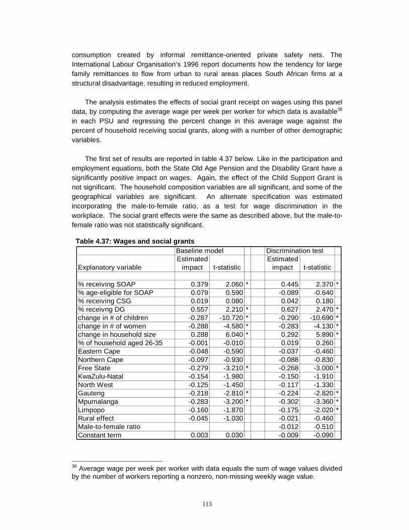
113
consumption created by informal remittance-oriented private safety nets. The International Labour Organisation’s 1996 report documents how the tendency for large family remittances to flow from urban to rural areas places South African firms at a structural disadvantage, resulting in reduced employment.
The analysis estimates the effects of social grant receipt on wages using this panel data, by computing the average wage per week per worker for which data is available38 in each PSU and regressing the percent change in this average wage against the percent of household receiving social grants, along with a number of other demographic variables.
The first set of results are reported in table 4.37 below. Like in the participation and employment equations, both the State Old Age Pension and the Disability Grant have a significantly positive impact on wages. Again, the effect of the Child Support Grant is not significant. The household composition variables are all significant, and some of the geographical variables are significant. An alternate specification was estimated incorporating the male-to-female ratio, as a test for wage discrimination in the workplace. The social grant effects were the same as described above, but the male-to-female ratio was not statistically significant. Table 4.37: Wages and social grants
38 Average wage per week per worker with data equals the sum of wage values divided by the number of workers reporting a nonzero, non-missing weekly wage value.
Baseline model Discrimination test
Explanatory variableEstimated
impact t-statisticEstimated
impact t-statistic
% receiving SOAP 0.379 2.060 * 0.445 2.370 *% age-eligible for SOAP 0.079 0.590 -0.089 -0.640% receiving CSG 0.019 0.080 0.042 0.180% receivng DG 0.557 2.210 * 0.627 2.470 *change in # of children -0.287 -10.720 * -0.290 -10.690 *change in # of women -0.288 -4.580 * -0.283 -4.130 *change in household size 0.288 6.040 * 0.292 5.890 *% of household aged 26-35 -0.001 -0.010 0.019 0.260Eastern Cape -0.048 -0.590 -0.037 -0.460Northern Cape -0.097 -0.930 -0.088 -0.830Free State -0.279 -3.210 * -0.268 -3.000 *KwaZulu-Natal -0.154 -1.980 -0.150 -1.910North West -0.125 -1.450 -0.117 -1.330Gauteng -0.218 -2.810 * -0.224 -2.820 *Mpumalanga -0.283 -3.200 * -0.302 -3.360 *Limpopo -0.160 -1.870 -0.175 -2.020 *Rural effect -0.045 -1.030 -0.021 -0.460Male-to-female ratio -0.012 -0.510Constant term 0.003 0.030 -0.009 -0.090
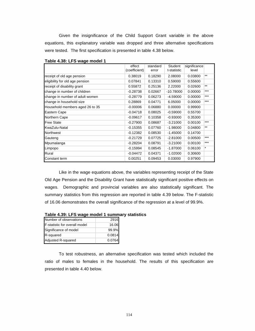
114
Given the insignificance of the Child Support Grant variable in the above
equations, this explanatory variable was dropped and three alternative specifications
were tested. The first specification is presented in table 4.38 below. Table 4.38: LFS wage model 1
effect (coefficient)
standard error
Student t-statistic
significance level
receipt of old age pension 0.38019 0.18290 2.08000 0.03800 ** eligibility for old age pension 0.07841 0.13310 0.59000 0.55600 receipt of disability grant 0.55872 0.25136 2.22000 0.02600 ** change in number of children -0.28738 0.02667 -10.78000 0.00000 *** change in number of adult women -0.28779 0.06273 -4.59000 0.00000 *** change in household size 0.28869 0.04771 6.05000 0.00000 *** Household members aged 26 to 35 -0.00006 0.06880 0.00000 0.99900 Eastern Cape -0.04718 0.08025 -0.59000 0.55700 Northern Cape -0.09617 0.10358 -0.93000 0.35300 Free State -0.27900 0.08687 -3.21000 0.00100 *** KwaZulu-Natal -0.15355 0.07760 -1.98000 0.04800 ** Northwest -0.12382 0.08530 -1.45000 0.14700 Gauteng -0.21729 0.07725 -2.81000 0.00500 *** Mpumalanga -0.28204 0.08791 -3.21000 0.00100 *** Limpopo -0.15994 0.08545 -1.87000 0.06100 * Rural -0.04472 0.04371 -1.02000 0.30600 Constant term 0.00251 0.09453 0.03000 0.97900
Like in the wage equations above, the variables representing receipt of the State
Old Age Pension and the Disability Grant have statistically significant positive effects on
wages. Demographic and provincial variables are also statistically significant. The
summary statistics from this regression are reported in table 4.39 below. The F-statistic
of 16.06 demonstrates the overall significance of the regression at a level of 99.9%.
Table 4.39: LFS wage model 1 summary statistics Number of observations 2916F-statistic for overall model 16.06Significance of model 99.9%R-squared 0.0814Adjusted R-squared 0.0764
To test robustness, an alternative specification was tested which included the
ratio of males to females in the household. The results of this specification are
presented in table 4.40 below.
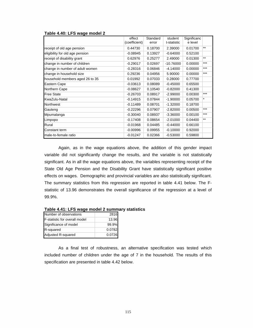
115
Table 4.40: LFS wage model 2 effect
(coefficient)Standard
error student
t-statistic Significanc
e level
receipt of old age pension 0.44730 0.18700 2.39000 0.01700 ** eligibility for old age pension -0.08945 0.13927 -0.64000 0.52100 receipt of disability grant 0.62976 0.25277 2.49000 0.01300 ** change in number of children -0.29017 0.02697 -10.76000 0.00000 *** change in number of adult women -0.28316 0.06846 -4.14000 0.00000 *** change in household size 0.29236 0.04956 5.90000 0.00000 *** household members aged 26 to 35 0.01992 0.07033 0.28000 0.77700 Eastern Cape -0.03613 0.08089 -0.45000 0.65500 Northern Cape -0.08627 0.10540 -0.82000 0.41300 Free State -0.26703 0.08917 -2.99000 0.00300 *** KwaZulu-Natal -0.14915 0.07844 -1.90000 0.05700 * Northwest -0.11489 0.08701 -1.32000 0.18700 Gauteng -0.22296 0.07907 -2.82000 0.00500 *** Mpumalanga -0.30040 0.08937 -3.36000 0.00100 *** Limpopo -0.17408 0.08654 -2.01000 0.04400 ** Rural -0.01968 0.04485 -0.44000 0.66100 Constant term -0.00996 0.09955 -0.10000 0.92000 male-to-female ratio -0.01247 0.02366 -0.53000 0.59800
Again, as in the wage equations above, the addition of this gender impact
variable did not significantly change the results, and the variable is not statistically significant. As in all the wage equations above, the variables representing receipt of the State Old Age Pension and the Disability Grant have statistically significant positive effects on wages. Demographic and provincial variables are also statistically significant. The summary statistics from this regression are reported in table 4.41 below. The F-statistic of 13.96 demonstrates the overall significance of the regression at a level of 99.9%. Table 4.41: LFS wage model 2 summary statistics Number of observations 2816F-statistic for overall model 13.96Significance of model 99.9%R-squared 0.0782Adjusted R-squared 0.0726
As a final test of robustness, an alternative specification was tested which
included number of children under the age of 7 in the household. The results of this specification are presented in table 4.42 below.
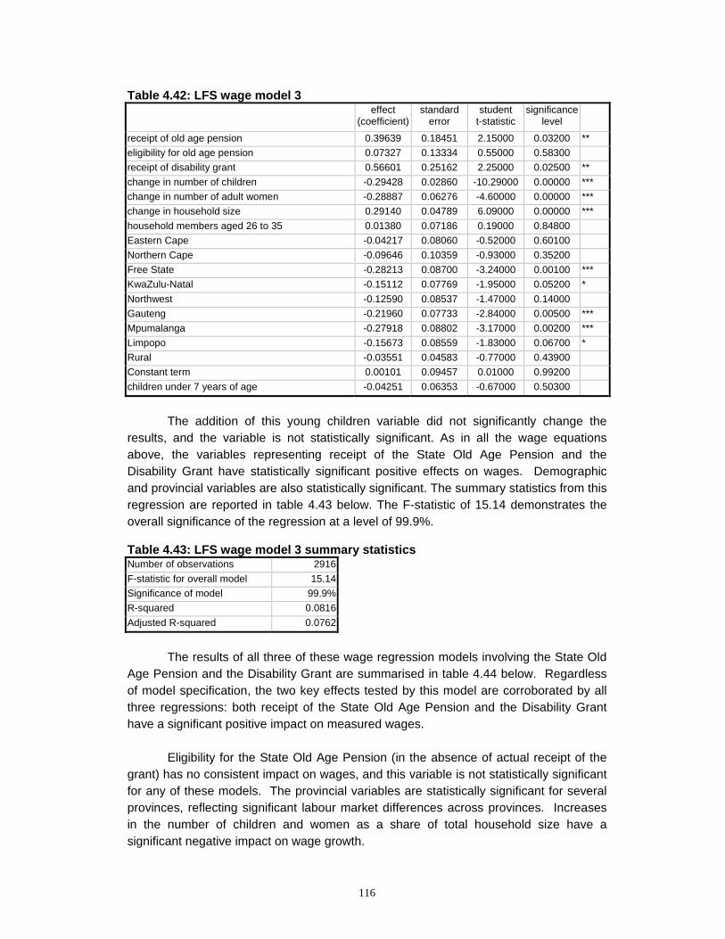
116
Table 4.42: LFS wage model 3 effect
(coefficient)standard
error student
t-statistic significance
level
receipt of old age pension 0.39639 0.18451 2.15000 0.03200 ** eligibility for old age pension 0.07327 0.13334 0.55000 0.58300 receipt of disability grant 0.56601 0.25162 2.25000 0.02500 ** change in number of children -0.29428 0.02860 -10.29000 0.00000 *** change in number of adult women -0.28887 0.06276 -4.60000 0.00000 *** change in household size 0.29140 0.04789 6.09000 0.00000 *** household members aged 26 to 35 0.01380 0.07186 0.19000 0.84800 Eastern Cape -0.04217 0.08060 -0.52000 0.60100 Northern Cape -0.09646 0.10359 -0.93000 0.35200 Free State -0.28213 0.08700 -3.24000 0.00100 *** KwaZulu-Natal -0.15112 0.07769 -1.95000 0.05200 * Northwest -0.12590 0.08537 -1.47000 0.14000 Gauteng -0.21960 0.07733 -2.84000 0.00500 *** Mpumalanga -0.27918 0.08802 -3.17000 0.00200 *** Limpopo -0.15673 0.08559 -1.83000 0.06700 * Rural -0.03551 0.04583 -0.77000 0.43900 Constant term 0.00101 0.09457 0.01000 0.99200 children under 7 years of age -0.04251 0.06353 -0.67000 0.50300
The addition of this young children variable did not significantly change the
results, and the variable is not statistically significant. As in all the wage equations above, the variables representing receipt of the State Old Age Pension and the Disability Grant have statistically significant positive effects on wages. Demographic and provincial variables are also statistically significant. The summary statistics from this regression are reported in table 4.43 below. The F-statistic of 15.14 demonstrates the overall significance of the regression at a level of 99.9%. Table 4.43: LFS wage model 3 summary statistics Number of observations 2916F-statistic for overall model 15.14Significance of model 99.9%R-squared 0.0816Adjusted R-squared 0.0762
The results of all three of these wage regression models involving the State Old
Age Pension and the Disability Grant are summarised in table 4.44 below. Regardless of model specification, the two key effects tested by this model are corroborated by all three regressions: both receipt of the State Old Age Pension and the Disability Grant have a significant positive impact on measured wages.
Eligibility for the State Old Age Pension (in the absence of actual receipt of the
grant) has no consistent impact on wages, and this variable is not statistically significant for any of these models. The provincial variables are statistically significant for several provinces, reflecting significant labour market differences across provinces. Increases in the number of children and women as a share of total household size have a significant negative impact on wage growth.
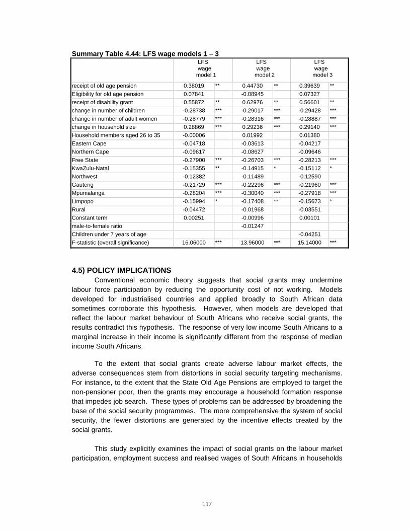
117
Summary Table 4.44: LFS wage models 1 – 3 LFS
wage model 1
LFS wage
model 2
LFS wage
model 3
receipt of old age pension 0.38019 ** 0.44730 ** 0.39639 ** Eligibility for old age pension 0.07841 -0.08945 0.07327 receipt of disability grant 0.55872 ** 0.62976 ** 0.56601 ** change in number of children -0.28738 *** -0.29017 *** -0.29428 *** change in number of adult women -0.28779 *** -0.28316 *** -0.28887 *** change in household size 0.28869 *** 0.29236 *** 0.29140 *** Household members aged 26 to 35 -0.00006 0.01992 0.01380 Eastern Cape -0.04718 -0.03613 -0.04217 Northern Cape -0.09617 -0.08627 -0.09646 Free State -0.27900 *** -0.26703 *** -0.28213 *** KwaZulu-Natal -0.15355 ** -0.14915 * -0.15112 * Northwest -0.12382 -0.11489 -0.12590 Gauteng -0.21729 *** -0.22296 *** -0.21960 *** Mpumalanga -0.28204 *** -0.30040 *** -0.27918 *** Limpopo -0.15994 * -0.17408 ** -0.15673 * Rural -0.04472 -0.01968 -0.03551 Constant term 0.00251 -0.00996 0.00101 male-to-female ratio -0.01247 Children under 7 years of age -0.04251 F-statistic (overall significance) 16.06000 *** 13.96000 *** 15.14000 ***
4.5) POLICY IMPLICATIONS
Conventional economic theory suggests that social grants may undermine labour force participation by reducing the opportunity cost of not working. Models developed for industrialised countries and applied broadly to South African data sometimes corroborate this hypothesis. However, when models are developed that reflect the labour market behaviour of South Africans who receive social grants, the results contradict this hypothesis. The response of very low income South Africans to a marginal increase in their income is significantly different from the response of median income South Africans.
To the extent that social grants create adverse labour market effects, the adverse consequences stem from distortions in social security targeting mechanisms. For instance, to the extent that the State Old Age Pensions are employed to target the non-pensioner poor, then the grants may encourage a household formation response that impedes job search. These types of problems can be addressed by broadening the base of the social security programmes. The more comprehensive the system of social security, the fewer distortions are generated by the incentive effects created by the social grants.
This study explicitly examines the impact of social grants on the labour market participation, employment success and realised wages of South Africans in households
118
receiving social grants. While statistical analysis cannot prove causation, the empirical results are consistent with the hypotheses that:
(4) Social grants provide potential labour market participants with the resources and economic security necessary to invest in high-risk/high-reward job search.
(5) Living in a household receiving social grants is correlated with a higher success rate in finding employment.
(6) Workers in households receiving social grants are better able to improve their productivity and as a result earn higher wage increases.
The empirical evidence discussed in this chapter demonstrates that people in
households receiving social grants have increased both their labour force participation and employment rates faster than those who live in households that do not receive social grants. In addition, workers in households receiving social grants have realised more rapid wage increases. These findings are consistent with the hypothesis that South Africa’s social grants increase both the supply and demand for labour. This suggests that South Africa’s system of social grants promotes employment creation.
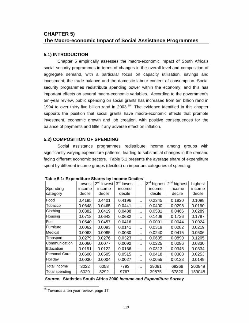
119
CHAPTER 5) The Macro-economic Impact of Social Assistance Programmes
5.1) INTRODUCTION Chapter 5 empirically assesses the macro-economic impact of South Africa's
social security programmes in terms of changes in the overall level and composition of aggregate demand, with a particular focus on capacity utilisation, savings and investment, the trade balance and the domestic labour content of consumption. Social security programmes redistribute spending power within the economy, and this has important effects on several macro-economic variables. According to the government’s ten-year review, public spending on social grants has increased from ten billion rand in 1994 to over thirty-five billion rand in 2003.39 The evidence identified in this chapter supports the position that social grants have macro-economic effects that promote investment, economic growth and job creation, with positive consequences for the balance of payments and little if any adverse effect on inflation. 5.2) COMPOSITION OF SPENDING
Social assistance programmes redistribute income among groups with significantly varying expenditure patterns, leading to substantial changes in the demand facing different economic sectors. Table 5.1 presents the average share of expenditure spent by different income groups (deciles) on important categories of spending. Table 5.1: Expenditure Shares by Income Deciles Spending category
Lowest income decile
2nd lowest income decile
3rd lowest income decile
… 3rd highest income decile
2nd highest income decile
highest income decile
Food 0.4185 0.4401 0.4196 … 0.2345 0.1820 0.1098 Tobacco 0.0648 0.0465 0.0441 … 0.0400 0.0298 0.0190 Clothing 0.0382 0.0419 0.0488 … 0.0581 0.0466 0.0289 Housing 0.0718 0.0642 0.0682 … 0.1406 0.1726 0.1797 Fuel 0.0540 0.0457 0.0416 … 0.0091 0.0044 0.0024 Furniture 0.0062 0.0093 0.0141 … 0.0319 0.0282 0.0219 Medical 0.0063 0.0085 0.0080 … 0.0240 0.0415 0.0506 Transport 0.0279 0.0276 0.0323 … 0.0685 0.0890 0.1205 Communication 0.0060 0.0077 0.0092 … 0.0225 0.0286 0.0330 Education 0.0191 0.0122 0.0166 … 0.0313 0.0345 0.0334 Personal Care 0.0600 0.0505 0.0515 … 0.0418 0.0368 0.0253 Holiday 0.0030 0.0004 0.0027 … 0.0055 0.0133 0.0149 Total income 3022 6058 7793 … 39091 69268 200949 Total spending 6029 8292 9767 … 39875 67820 189048
Source: Statistics South Africa 2000 Income and Expenditure Survey 39 Towards a ten year review, page 17.
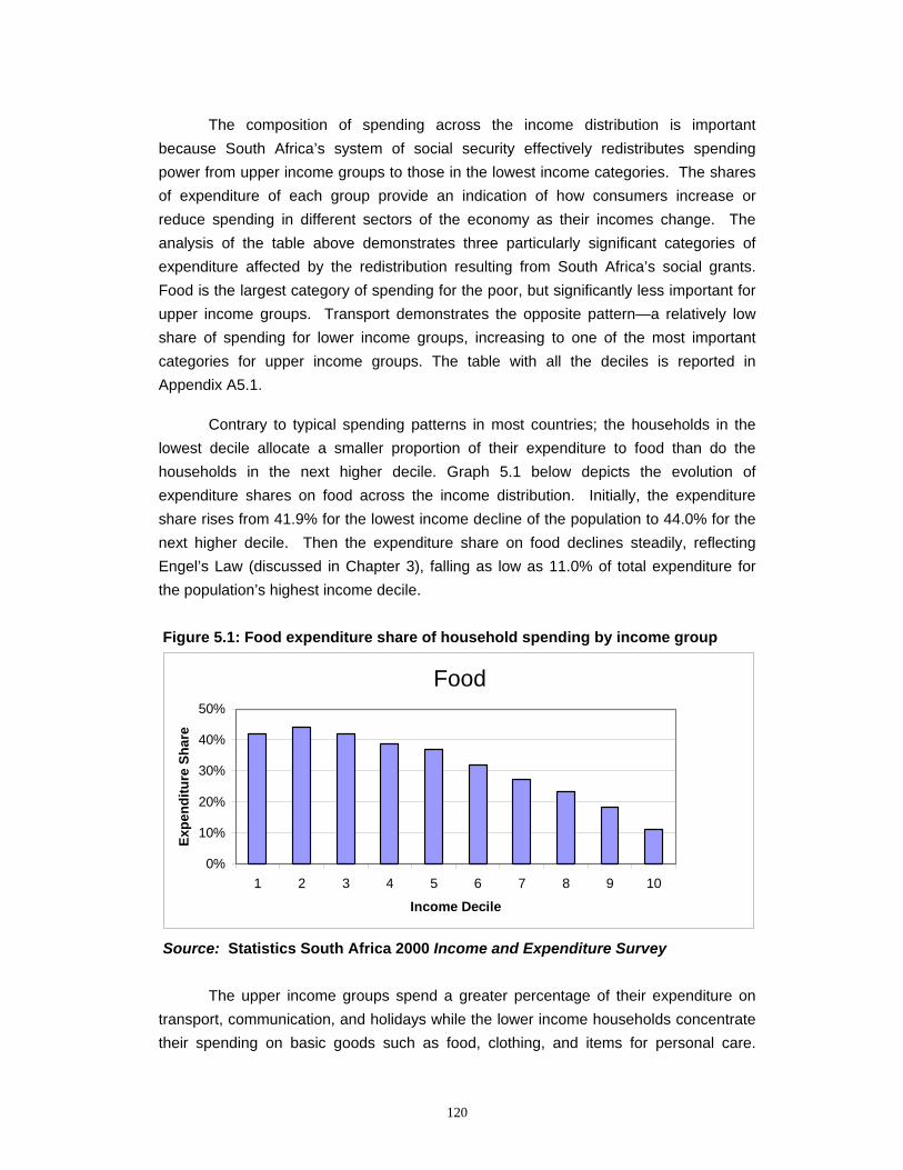
120
The composition of spending across the income distribution is important because South Africa’s system of social security effectively redistributes spending power from upper income groups to those in the lowest income categories. The shares of expenditure of each group provide an indication of how consumers increase or reduce spending in different sectors of the economy as their incomes change. The analysis of the table above demonstrates three particularly significant categories of expenditure affected by the redistribution resulting from South Africa’s social grants. Food is the largest category of spending for the poor, but significantly less important for upper income groups. Transport demonstrates the opposite pattern—a relatively low share of spending for lower income groups, increasing to one of the most important categories for upper income groups. The table with all the deciles is reported in Appendix A5.1.
Contrary to typical spending patterns in most countries; the households in the lowest decile allocate a smaller proportion of their expenditure to food than do the households in the next higher decile. Graph 5.1 below depicts the evolution of expenditure shares on food across the income distribution. Initially, the expenditure share rises from 41.9% for the lowest income decline of the population to 44.0% for the next higher decile. Then the expenditure share on food declines steadily, reflecting Engel’s Law (discussed in Chapter 3), falling as low as 11.0% of total expenditure for the population’s highest income decile. Figure 5.1: Food expenditure share of household spending by income group
Source: Statistics South Africa 2000 Income and Expenditure Survey
The upper income groups spend a greater percentage of their expenditure on
transport, communication, and holidays while the lower income households concentrate their spending on basic goods such as food, clothing, and items for personal care.
Food
0%
10%
20%
30%
40%
50%
1 2 3 4 5 6 7 8 9 10
Income Decile
Expe
nditu
re S
hare
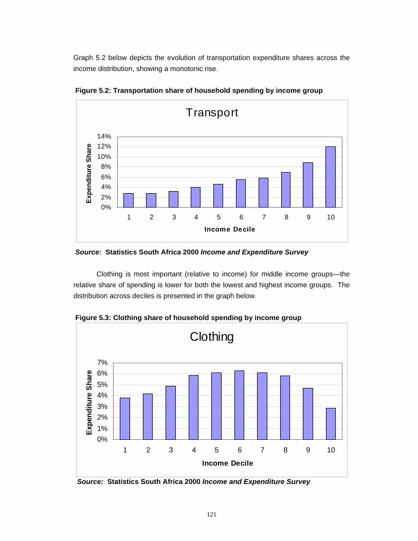
121
Graph 5.2 below depicts the evolution of transportation expenditure shares across the income distribution, showing a monotonic rise.
Figure 5.2: Transportation share of household spending by income group
Source: Statistics South Africa 2000 Income and Expenditure Survey
Clothing is most important (relative to income) for middle income groups—the relative share of spending is lower for both the lowest and highest income groups. The distribution across deciles is presented in the graph below.
Figure 5.3: Clothing share of household spending by income group
Source: Statistics South Africa 2000 Income and Expenditure Survey
Transport
0%2%4%6%8%
10%12%14%
1 2 3 4 5 6 7 8 9 10
Income Decile
Expe
nditu
re S
hare
Clothing
0%1%2%3%4%5%6%7%
1 2 3 4 5 6 7 8 9 10
Income Decile
Expe
nditu
re S
hare
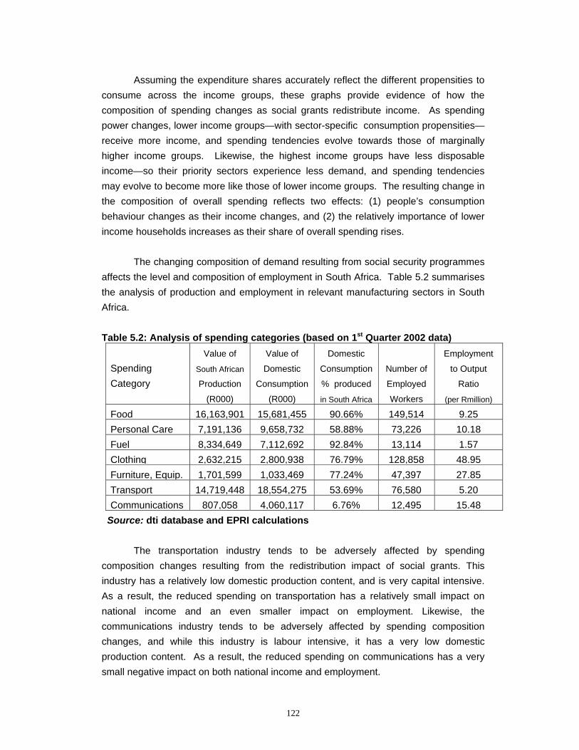
122
Assuming the expenditure shares accurately reflect the different propensities to consume across the income groups, these graphs provide evidence of how the composition of spending changes as social grants redistribute income. As spending power changes, lower income groups—with sector-specific consumption propensities—receive more income, and spending tendencies evolve towards those of marginally higher income groups. Likewise, the highest income groups have less disposable income—so their priority sectors experience less demand, and spending tendencies may evolve to become more like those of lower income groups. The resulting change in the composition of overall spending reflects two effects: (1) people’s consumption behaviour changes as their income changes, and (2) the relatively importance of lower income households increases as their share of overall spending rises.
The changing composition of demand resulting from social security programmes affects the level and composition of employment in South Africa. Table 5.2 summarises the analysis of production and employment in relevant manufacturing sectors in South Africa. Table 5.2: Analysis of spending categories (based on 1st Quarter 2002 data)
Spending Category
Value of
South African
Production
(R000)
Value of
Domestic
Consumption
(R000)
Domestic
Consumption
% produced
in South Africa
Number of
Employed
Workers
Employment
to Output
Ratio
(per Rmillion)
Food 16,163,901 15,681,455 90.66% 149,514 9.25Personal Care 7,191,136 9,658,732 58.88% 73,226 10.18Fuel 8,334,649 7,112,692 92.84% 13,114 1.57Clothing 2,632,215 2,800,938 76.79% 128,858 48.95Furniture, Equip. 1,701,599 1,033,469 77.24% 47,397 27.85Transport 14,719,448 18,554,275 53.69% 76,580 5.20Communications 807,058 4,060,117 6.76% 12,495 15.48
Source: dti database and EPRI calculations
The transportation industry tends to be adversely affected by spending composition changes resulting from the redistribution impact of social grants. This industry has a relatively low domestic production content, and is very capital intensive. As a result, the reduced spending on transportation has a relatively small impact on national income and an even smaller impact on employment. Likewise, the communications industry tends to be adversely affected by spending composition changes, and while this industry is labour intensive, it has a very low domestic production content. As a result, the reduced spending on communications has a very small negative impact on both national income and employment.
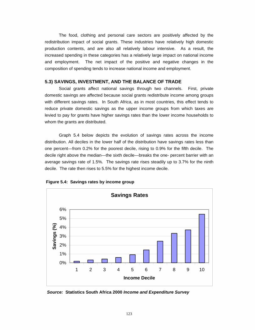
123
The food, clothing and personal care sectors are positively affected by the redistribution impact of social grants. These industries have relatively high domestic production contents, and are also all relatively labour intensive. As a result, the increased spending in these categories has a relatively large impact on national income and employment. The net impact of the positive and negative changes in the composition of spending tends to increase national income and employment. 5.3) SAVINGS, INVESTMENT, AND THE BALANCE OF TRADE
Social grants affect national savings through two channels. First, private domestic savings are affected because social grants redistribute income among groups with different savings rates. In South Africa, as in most countries, this effect tends to reduce private domestic savings as the upper income groups from which taxes are levied to pay for grants have higher savings rates than the lower income households to whom the grants are distributed.
Graph 5.4 below depicts the evolution of savings rates across the income distribution. All deciles in the lower half of the distribution have savings rates less than one percent—from 0.2% for the poorest decile, rising to 0.9% for the fifth decile. The decile right above the median—the sixth decile—breaks the one- percent barrier with an average savings rate of 1.5%. The savings rate rises steadily up to 3.7% for the ninth decile. The rate then rises to 5.5% for the highest income decile. Figure 5.4: Savings rates by income group
Source: Statistics South Africa 2000 Income and Expenditure Survey
Savings Rates
0%
1%
2%
3%
4%
5%
6%
1 2 3 4 5 6 7 8 9 10
Income Decile
Savi
ngs
(%)
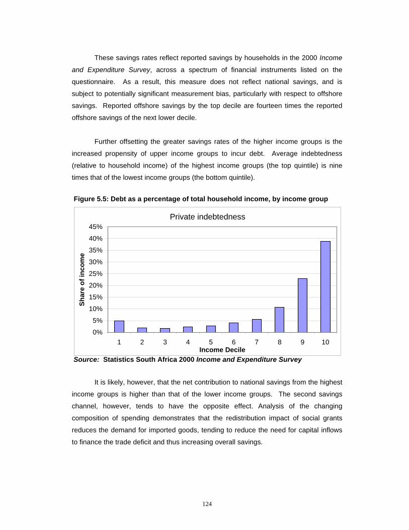
124
These savings rates reflect reported savings by households in the 2000 Income
and Expenditure Survey, across a spectrum of financial instruments listed on the
questionnaire. As a result, this measure does not reflect national savings, and is
subject to potentially significant measurement bias, particularly with respect to offshore
savings. Reported offshore savings by the top decile are fourteen times the reported
offshore savings of the next lower decile.
Further offsetting the greater savings rates of the higher income groups is the
increased propensity of upper income groups to incur debt. Average indebtedness
(relative to household income) of the highest income groups (the top quintile) is nine
times that of the lowest income groups (the bottom quintile). Figure 5.5: Debt as a percentage of total household income, by income group Source: Statistics South Africa 2000 Income and Expenditure Survey
It is likely, however, that the net contribution to national savings from the highest
income groups is higher than that of the lower income groups. The second savings
channel, however, tends to have the opposite effect. Analysis of the changing
composition of spending demonstrates that the redistribution impact of social grants
reduces the demand for imported goods, tending to reduce the need for capital inflows
to finance the trade deficit and thus increasing overall savings.
Private indebtedness
0%
5%
10%
15%
20%
25%
30%
35%
40%
45%
1 2 3 4 5 6 7 8 9 10Income Decile
Shar
e of
inco
me
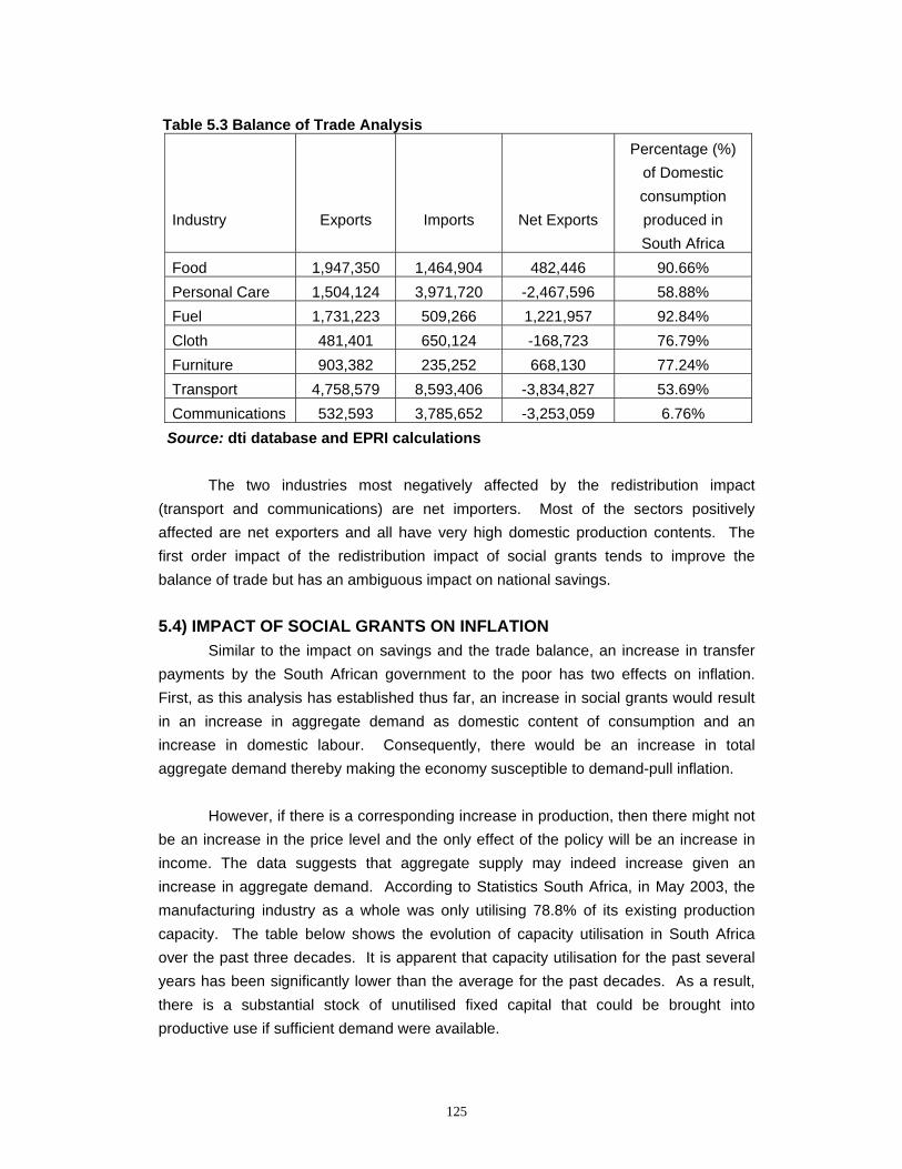
125
Table 5.3 Balance of Trade Analysis Industry
Exports
Imports
Net Exports
Percentage (%) of Domestic consumption produced in South Africa
Food 1,947,350 1,464,904 482,446 90.66% Personal Care 1,504,124 3,971,720 -2,467,596 58.88% Fuel 1,731,223 509,266 1,221,957 92.84% Cloth 481,401 650,124 -168,723 76.79% Furniture 903,382 235,252 668,130 77.24% Transport 4,758,579 8,593,406 -3,834,827 53.69% Communications 532,593 3,785,652 -3,253,059 6.76%
Source: dti database and EPRI calculations
The two industries most negatively affected by the redistribution impact (transport and communications) are net importers. Most of the sectors positively affected are net exporters and all have very high domestic production contents. The first order impact of the redistribution impact of social grants tends to improve the balance of trade but has an ambiguous impact on national savings. 5.4) IMPACT OF SOCIAL GRANTS ON INFLATION
Similar to the impact on savings and the trade balance, an increase in transfer payments by the South African government to the poor has two effects on inflation. First, as this analysis has established thus far, an increase in social grants would result in an increase in aggregate demand as domestic content of consumption and an increase in domestic labour. Consequently, there would be an increase in total aggregate demand thereby making the economy susceptible to demand-pull inflation.
However, if there is a corresponding increase in production, then there might not be an increase in the price level and the only effect of the policy will be an increase in income. The data suggests that aggregate supply may indeed increase given an increase in aggregate demand. According to Statistics South Africa, in May 2003, the manufacturing industry as a whole was only utilising 78.8% of its existing production capacity. The table below shows the evolution of capacity utilisation in South Africa over the past three decades. It is apparent that capacity utilisation for the past several years has been significantly lower than the average for the past decades. As a result, there is a substantial stock of unutilised fixed capital that could be brought into productive use if sufficient demand were available.
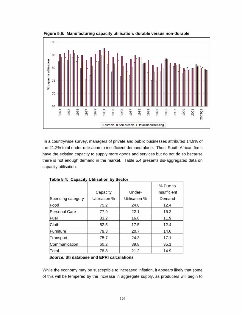
126
Figure 5.6: Manufacturing capacity utilisation: durable versus non-durable In a countrywide survey, managers of private and public businesses attributed 14.9% of the 21.2% total under-utilisation to insufficient demand alone. Thus, South African firms have the existing capacity to supply more goods and services but do not do so because there is not enough demand in the market. Table 5.4 presents dis-aggregated data on capacity utilisation. Table 5.4: Capacity Utilisation by Sector
Spending category
Capacity
Utilisation %
Under-
Utilisation %
% Due to Insufficient Demand
Food 75.2 24.8 12.4 Personal Care 77.9 22.1 16.2 Fuel 83.2 16.8 11.9 Cloth 82.5 17.5 12.4 Furniture 79.3 20.7 14.6 Transport 75.7 24.3 17.1 Communication 60.2 39.8 35.1 Total 78.8 21.2 14.9
Source: dti database and EPRI calculations While the economy may be susceptible to increased inflation, it appears likely that some of this will be tempered by the increase in aggregate supply, as producers will begin to
65
70
75
80
85
90
1971
1973
1975
1977
1979
1981
1983
1985
1987
1989
1991
1993
1995
1997
1999
2001
2003
Q1
% c
apac
ity u
tilis
atio
n
durable non-durable total manufacturing
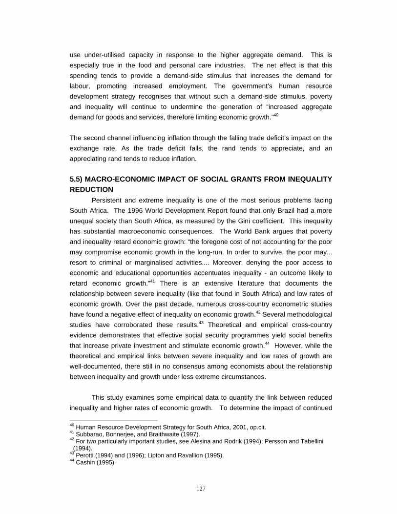
127
use under-utilised capacity in response to the higher aggregate demand. This is especially true in the food and personal care industries. The net effect is that this spending tends to provide a demand-side stimulus that increases the demand for labour, promoting increased employment. The government’s human resource development strategy recognises that without such a demand-side stimulus, poverty and inequality will continue to undermine the generation of “increased aggregate demand for goods and services, therefore limiting economic growth.”40 The second channel influencing inflation through the falling trade deficit’s impact on the exchange rate. As the trade deficit falls, the rand tends to appreciate, and an appreciating rand tends to reduce inflation. 5.5) MACRO-ECONOMIC IMPACT OF SOCIAL GRANTS FROM INEQUALITY REDUCTION
Persistent and extreme inequality is one of the most serious problems facing South Africa. The 1996 World Development Report found that only Brazil had a more unequal society than South Africa, as measured by the Gini coefficient. This inequality has substantial macroeconomic consequences. The World Bank argues that poverty and inequality retard economic growth: “the foregone cost of not accounting for the poor may compromise economic growth in the long-run. In order to survive, the poor may... resort to criminal or marginalised activities.... Moreover, denying the poor access to economic and educational opportunities accentuates inequality - an outcome likely to retard economic growth.”41 There is an extensive literature that documents the relationship between severe inequality (like that found in South Africa) and low rates of economic growth. Over the past decade, numerous cross-country econometric studies have found a negative effect of inequality on economic growth.42 Several methodological studies have corroborated these results.43 Theoretical and empirical cross-country evidence demonstrates that effective social security programmes yield social benefits that increase private investment and stimulate economic growth.44 However, while the theoretical and empirical links between severe inequality and low rates of growth are well-documented, there still in no consensus among economists about the relationship between inequality and growth under less extreme circumstances.
This study examines some empirical data to quantify the link between reduced inequality and higher rates of economic growth. To determine the impact of continued
40 Human Resource Development Strategy for South Africa, 2001, op.cit. 41 Subbarao, Bonnerjee, and Braithwaite (1997). 42 For two particularly important studies, see Alesina and Rodrik (1994); Persson and Tabellini (1994). 43 Perotti (1994) and (1996); Lipton and Ravallion (1995). 44 Cashin (1995).
128
inequality on the macro-economy, this study analyses growth rates and inequality measures (Gini coefficients) “for those countries for which reliable data are available.”45 The analysis shows that high Gini coefficients are significantly correlated with low rates of economic growth, as depicted in the graph below. Figure 5.7: Initial inequality and subsequent economic growth Source: Hoeven (2001) and EPRI calculations
A simple linear regression of cross-country Gini coefficients against growth rates estimates that a 1% decrease in the Gini is associated with a 0.12% increase in growth. (This result was statistically significant at the 90% level. The data for this regression are reported in Appendix A5.2.) These findings are corroborated by a multitude of papers that identify similar results. Studies “run over a variety of data sets and periods with many different measures of income distribution, deliver a consistent message: initial inequality is detrimental to long-run growth” (Benabou 2003). For additional studies that document a significant negative relationship between inequality and growth, see Alesina-Rodrick (1994), Clarke (1992), Perotti (1992, 1994, 1996), Persoson-Tabellini (1992, 1994), and Venieris-Gupta (1986).
An increased take-up in social grants, then, would have the effect of reducing
South Africa’s Gini coefficient as the income differentials across the income distribution
would be reduced. A redistribution programme that pays for these grants with increased
taxes would have an even more pronounced effect because the disposable income of 45 van der Hoeven (2001).
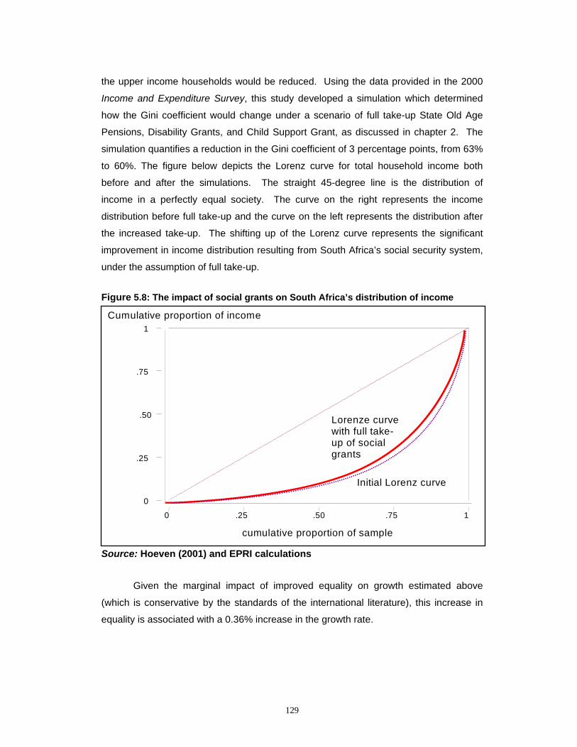
129
the upper income households would be reduced. Using the data provided in the 2000
Income and Expenditure Survey, this study developed a simulation which determined
how the Gini coefficient would change under a scenario of full take-up State Old Age
Pensions, Disability Grants, and Child Support Grant, as discussed in chapter 2. The
simulation quantifies a reduction in the Gini coefficient of 3 percentage points, from 63%
to 60%. The figure below depicts the Lorenz curve for total household income both
before and after the simulations. The straight 45-degree line is the distribution of
income in a perfectly equal society. The curve on the right represents the income
distribution before full take-up and the curve on the left represents the distribution after
the increased take-up. The shifting up of the Lorenz curve represents the significant
improvement in income distribution resulting from South Africa’s social security system,
under the assumption of full take-up. Figure 5.8: The impact of social grants on South Africa’s distribution of income - Source: Hoeven (2001) and EPRI calculations
Given the marginal impact of improved equality on growth estimated above
(which is conservative by the standards of the international literature), this increase in
equality is associated with a 0.36% increase in the growth rate.
cumulative proportion of sample
0 .25 .50 .75 1
0
.25
.50
.75
1Cumulative proportion of income
Initial Lorenz curve
Lorenze curvewith full take-up of socialgrants
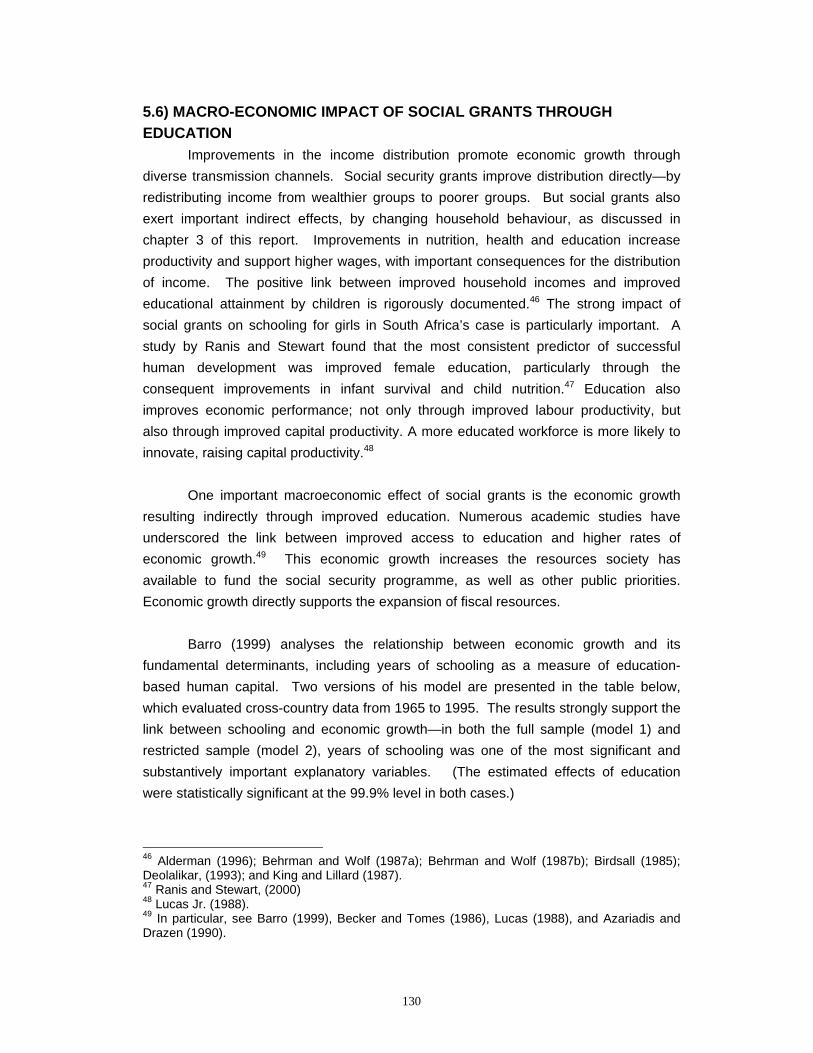
130
5.6) MACRO-ECONOMIC IMPACT OF SOCIAL GRANTS THROUGH EDUCATION
Improvements in the income distribution promote economic growth through diverse transmission channels. Social security grants improve distribution directly—by redistributing income from wealthier groups to poorer groups. But social grants also exert important indirect effects, by changing household behaviour, as discussed in chapter 3 of this report. Improvements in nutrition, health and education increase productivity and support higher wages, with important consequences for the distribution of income. The positive link between improved household incomes and improved educational attainment by children is rigorously documented.46 The strong impact of social grants on schooling for girls in South Africa’s case is particularly important. A study by Ranis and Stewart found that the most consistent predictor of successful human development was improved female education, particularly through the consequent improvements in infant survival and child nutrition.47 Education also improves economic performance; not only through improved labour productivity, but also through improved capital productivity. A more educated workforce is more likely to innovate, raising capital productivity.48
One important macroeconomic effect of social grants is the economic growth resulting indirectly through improved education. Numerous academic studies have underscored the link between improved access to education and higher rates of economic growth.49 This economic growth increases the resources society has available to fund the social security programme, as well as other public priorities. Economic growth directly supports the expansion of fiscal resources.
Barro (1999) analyses the relationship between economic growth and its fundamental determinants, including years of schooling as a measure of education-based human capital. Two versions of his model are presented in the table below, which evaluated cross-country data from 1965 to 1995. The results strongly support the link between schooling and economic growth—in both the full sample (model 1) and restricted sample (model 2), years of schooling was one of the most significant and substantively important explanatory variables. (The estimated effects of education were statistically significant at the 99.9% level in both cases.)
46 Alderman (1996); Behrman and Wolf (1987a); Behrman and Wolf (1987b); Birdsall (1985); Deolalikar, (1993); and King and Lillard (1987). 47 Ranis and Stewart, (2000) 48 Lucas Jr. (1988). 49 In particular, see Barro (1999), Becker and Tomes (1986), Lucas (1988), and Azariadis and Drazen (1990).

131
Table 5.5: The Barro model of economic growth
SOURCE: Barro (1999)
Likewise, Gylfason (2000, 2001a) has quantified the link between improvements in educational outcomes and economic growth. Recognising that secondary school enrolment rates are imperfect yet common measures of human capital accumulation, Gylfason tests and confirms that primary and tertiary enrolment rates, years of school and education expenditure indicators yield similar results. His model explains economic growth with a simpler set of explanatory variables than those employed by Barro—Gylfason focuses on education, natural capital, human capital (education), physical capital and initial levels of income. The model is presented in the table below. All the explanatory variables are statistically significant at the 99.9% level. Initial income and natural capital are associated with lower growth rates, while investment and enrolment rates are associated with higher investment rates. The second model excludes education from the specification in order to test its incremental impact—enrolment rates explain fifteen percent of the variability in growth rates. Table 5.6:The Gylfason model of economic growth
The graph below depicts the positive relationship between adjusted growth rates (excluding the effect of initial income levels) and the secondary school enrolment rates. The simple correlation is also statistically significant, and illustrates South Africa’s position in the cross-country analysis. The data underlying this graph are reported in Appendix A5.3.
Explanatory variable Coefficient t-statistic Coefficient t-statisticlog(per capita GDP) 0.1240 4.59 0.1030 3.43log(per capita GDP) squared -0.0095 -5.28 -0.0082 -4.32govt. consumption/GDP -0.1490 -6.48 -0.1530 -5.67rule-of-law index 0.0172 3.25 0.0102 1.57democracy index 0.0540 1.86 0.0430 1.30democracy index squared -0.0480 -1.85 -0.0380 -1.36inflation rate -0.0370 -3.70 -0.0140 -1.56years of schooling 0.0072 4.24 0.0066 3.88log(total fertility rate) -0.0251 -5.34 -0.0306 -5.67investment/GDP 0.0590 2.68 0.0620 2.95growth rate of terms of trade 0.1650 5.89 0.1240 3.54
MODEL 1 MODEL 2
Explanatory variable Coefficient t-statistic Coefficient t-statisticConstant 9.35 6.00 3.87 2.50Natural capital -0.06 4.30 -0.09 5.70Enrolment rate 0.04 5.90Investment 0.07 3.10 0.13 4.50Initial income -1.40 7.00 -0.51 3.20R-squared
MODEL 1 MODEL 2
0.64 0.49
132
Figure 5.9: The relationship between education and growth SOURCE: Gylfason (2001) 5.7) CONCLUSION
At the macro-economic level, South Africa’s system of social development grants tends to increase domestic employment while promoting a more equal distribution of income. The effects of grants on national savings and the trade balance are ambiguous, since grants have two competing effects on the national savings—one through private domestic savings, and the other through the trade deficit. Depending on the magnitude of the effects, grants could improve or worsen national savings and the trade balance. Initial analysis suggests that the impact on savings may be negative, while that on the trade balance may be positive. However, since much of the savings of upper income groups are offshore, the negative impact is unlikely to be significant, particularly given the small share of private savings in the national savings rate. The impact on inflation may also be ambiguous. The increase in overall demand in the economy may generate some inflationary pressure. However, the relatively low rate of capacity utilisation may enable the economy to meet this demand without significant increases in inflation. Likewise, the positive trade balance effects may lead to an appreciation of the rand, tending to dampen imported inflation. On balance, the macro-economic impact of South Africa’s social security system is largely positive. These positive macroeconomic effects support higher rates of economic growth, which are re-inforced by the social security system’s positive effects on income distribution and education.
-6
-4
-2
0
2
4
6
0 20 40 60 80 100 120
Gross secondary-school enrolment 1980-97 (%)
Ann
ual g
row
th o
f GN
P pe
r cap
ita 1
965-
98
South Africa

133
CHAPTER 6) Summary, Conclusions and Policy Implications
This study documents how South Africa’s social assistance grants play a vital role in reducing poverty and promoting social development. The key findings are summarised and discussed below. 6.1) THE IMPACT ON POVERTY
South Africa’s social grants successfully reduce poverty, regardless of which methodology is used to quantify the impact measure or identify the poverty line. Nevertheless, the quantitative measure of poverty reduction is sensitive to the methodological choices. For instance, the measured impact is consistently greatest when employing the total rand poverty gap as an indicator. The poverty headcount measure, however, consistently yields the smallest results. Likewise, the choice of poverty line heavily influences the measurement of the quantitative impact. The current social security system is most successful when measured against destitution, and the impact is smallest when poverty lines ignore economies of scale and adult equivalence issues. For instance, South Africa’s social grants reduce the poverty headcount measure by 4.3%, as measured against the Committee of Inquiry’s expenditure poverty line (with no scales). The social security system, however, reduces 45% of the total rand destitution gap—an impact more than ten times greater.
Using the Committee of Inquiry expenditure poverty line (without scales), a 10% increase in take-up of the SOAP reduces the poverty gap by only 1.2%, and full take-up by only 2.5%. The take-up rate for the SOAP is already very high, and many of the eligible elderly not already receiving the SOAP are not among the poorest South Africans. As a result, further extensions of the SOAP have limited potential in reducing poverty. Extensions of the Disability Grant offer greater promise, although at substantially greater expense. A 50% increase in DG take-up reduces the total rand poverty gap by 1.7%, and full take-up generates a 5.1% reduction. The greatest poverty reducing potential lies with the progressive extension of the Child Support Grant. Extending the eligibility age to 14 reduces the poverty gap by 16.6%, and a further extension to age 18 reduces the gap by 21.4%. Increasing the real grant payment (as the government did in 2003) generates an even greater impact. The extension to age 14 yields a 22% poverty gap reduction, while the extension to age 18 reduces the poverty gap by 28.3%. Combining the higher CSG extended to age 14 with the full take-up of the SOAP and the DG yields a reduction in the total rand poverty gap of 29%.
The evidence in this report documents the substantial impact of South Africa’s social security system in reducing poverty and destitution. The magnitudes of the results are sensitive to methodological issues. It matters whether the poverty line is relative or absolute, whether it is scaled for household composition and economies of scale or not, and to a small extent whether it measures income or expenditure. Likewise, it matters how the poverty impact is measured—using poverty headcount or variants on the poverty gap. Nevertheless, the qualitative results, and the answers to critical policy questions, are robust to different methodological approaches. South Africa’s system of social security substantially reduces deprivation, and the progressive extension of the magnitude, scope and reach of social grants holds the potential to dramatically diminish the prevalence of poverty in South Africa.
134
6.2) THE IMPACT ON HOUSEHOLD WELL-BEING The results of this study provide evidence that the household impacts of South
Africa’s social grants are developmental in nature. These findings are consistent with international lessons of experience, as well as with previous studies of South Africa’s system of social security.
Poverty and its associated consequences erode the opportunities for children and youth to attend school, fomenting a vicious cycle of destitution by undermining the household’s capacity to accumulate the human capital necessary to break the poverty trap. Children in households that receive social grants, however, are more likely to attend school. Spending in these households focuses more strongly on basic needs, like food, fuel, housing and household operations, and less is spent on tobacco and debt. In case after case in this study, household outcomes conflicted with the simple implications of monetary income rankings. While many measures of well-being are correlated with aggregate income and expenditure, the exceptions affect large numbers of people and require careful policy analysis. The evidence in this report underscores the importance of moving beyond measures of income poverty in the assessment of social deprivation. 6.3) THE LABOUR MARKET IMPACT
This study explicitly examines the impact of social grants on the labour market participation, employment success and realised wages of South Africans in households receiving social grants. While statistical analysis cannot prove causation, the empirical results are consistent with the hypotheses that: (1) Social grants provide potential labour market participants with the resources and economic security necessary to invest in high-risk/high-reward job search. (2) Living in a household receiving social grants is correlated with a higher success rate in finding employment. (3) Workers in households receiving social grants are better able to improve their productivity and as a result earn higher wage increases.
The empirical evidence discussed in this chapter demonstrates that people in households receiving social grants have increased both their labour force participation and employment rates faster than those who live in households that do not receive social grants. In addition, workers in households receiving social grants have realised more rapid wage increases. These findings are consistent with the hypothesis that South Africa’s social grants increase both the supply and demand for labour. This evidence does not support the hypothesis that South Africa’s system of social grants negatively affects employment creation. 6.4) THE MACRO-ECONOMIC IMPACT
At the macro-economic level, South Africa’s system of social development grants tends to increase domestic employment while promoting a more equal distribution of income. The effects of grants on national savings and the trade balance are ambiguous, since grants have two competing effects on the national savings—one through private domestic savings, and the other through the trade deficit. Depending on the magnitude of the effects, grants could improve or worsen national savings and the trade balance. Initial analysis suggests that the impact on savings may be negative, while that on the trade balance may be positive. However, since much of the savings of upper income groups are offshore, the negative impact is unlikely to be significant, particularly given the small share of private savings in the national savings rate. The impact on inflation may also be ambiguous. The increase in overall demand in the economy may generate some inflationary pressure. However, the relatively low rate of capacity utilisation may
135
enable the economy to meet this demand without significant increases in inflation. Likewise, the positive trade balance effects may lead to an appreciation of the rand, tending to dampen imported inflation. On balance, the macro-economic impact of South Africa’s social security system is largely positive. These positive macroeconomic effects support higher rates of economic growth, which are re-inforced by the social security system’s positive effects on income distribution and education.
136
REFERENCES Alderman, H. “Saving and Economic Shocks in Rural Pakistan”, in Journal of Development Economics, Vol. 51. No. 2. pp. 346-65 (1996); Anderson, Kermyt G. “Family Structure, Parental Investment, And Educational Outcomes Among Black South Africans.” April 5, 2001. http://www.psc.isr.umich.edu/~kganders/workingpap/safr_famstruc.pdf. Aghion, Philippe, Eve Caroli, and Cecilia García-Peñalosa (1999), “Inequality and Economic Growth: The Perspective of the New Growth Theories,” Journal of Economic Literature 37, December, 1615-1660. Azariadis, C., Drazen, A., 1990, Threshold externalities in economic development, Quarterly Journal of Economics 105, 501-526. Ardington, Elisabeth and Lund, Frances. 1995. “Pensions and development: How the social security system can complement programmes of reconstruction and development”. Durban (Development Bank of Southern Africa). (Development Paper 61 Occasional paper.) p. 28. Barker, Frans. 1999. The South African Labour Market. Pretoria: J.L. van Schaik Publishers. p.118. Barrientos, Armando and Lloyd-Sherlock, Peter. 2002. "Non-Contributory Pensions and Social Protection." Social Protection Sector, International Labour Organization Barro, Robert J. 1997. The Determinants of Economic Growth, MIT Press, Cambridge, Massachusetts Barro, Robert, 1999. “Inequality, Growth and Investment.” National Bureau of Economic Research Working Paper #7038. Becker, G.S., Tomes, N., 1986, Human capital and the rise and fall of families, Journal of Labour Economics 4(3), S1-39. Behrman, Jere and Wolfe, Barbara. 1987a. “How Does Mother’s Schooling Affect the Family’s Health, Nutrition, Medical Care Usage and Household?” Journal of Econometrics. Behrman, J. and B. Wolf, “Investments in Schooling in Two Generations in Pre- Revolutionary Nicaragua”, in Journal of Development Economics, 27. pp. 395-419, 1987b; Bertrand, M, Miller, D. and S. Mullainathan 2000. Public Policy and Extended Families: Evidence from South Africa. National Bureau of Economic Research Working Paper 7594. Cambridge, Mass. Bhorat, H and M. Leibbrandt 2001. Modelling Vulnerability and Low Earnings in the South African Labour Market. Fighting Poverty: Labour Markets and Inequality in South Africa: Cape Town: UCT Press. 107-129.
137
Birdsall, Nancy. 1985. "Public Inputs and Child Schooling in Brazil". Journal of Development Economics. Vol. 18. pp. 67-86. Bouis, H.E. and Haddad, L.J. 1992. “Are estimates of calorie-income elasticities too high? A recalibration of the plausible range.” Journal of Development Economics. Vol. 39. Budlender, Debbie. 1993. “Women and household food security”. Cape Town. Printed for private circulation. Burgess, Robin; Stern, Nicholas. “Social Security in Developing Countries” What, Why, Who, and How?” in Social Security in Developing Countries. Clarendon Press, Oxford 1991. Pp41-80. Cameron, N. 1996. “Antenatal growth and birth factors and their relationships to child growth”. In Long-term Consequences of Early Environment. Edited by C. Jeya K. Henry and Stanley J. Ulijaszek. Cambridge: Cambridge University Press. Case, Ann and Deaton, Angus. 1996. "Large cash transfers to the elderly in South Africa". NBER Working Paper Series. No. W5572. pp. 7, 23-24. Case, Ann and Deaton, Angus. 1998. "Large cash transfers to the elderly in South Africa". The Economic Journal. Vol. 108. No. 450. pp. 1330-1361. Case, Anne. “The Primacy of Education.” Research Program in Development Studies, Princeton University. June 2001. http://www.wws.princeton.edu/~rpds/primacy-of-edu.pdf. Case, Anne. "Does Money Protect Health Status? Evidence from South African Pensions" NBER Working Paper , 2001. Case Anne, and Angus Deaton. "Consumption, health, gender and poverty." Princeton University, 2002. Cashin, Paul. 1995. “Government Spending, Taxes and Economic Growth.” IMF Staff Papers. Vol. 42, No.2. International Monetary Fund. p. 262. Castro, Leal; Florencia et- al. “Public Social Spending in Africa: Do the Poor Benefit?” World Bank Research Observer. 14(1), February 1999, Pgs. 49-72. “Child Health and Household Resources in South Africa: Evidence from the Old Age Pension Program” American Economic Review, May2000, Vol. 90 Issue 2, p393 Deolalikar, A.B. “Gender Differences in the Returns to Schooling and Schooling Enrollment Rates in Indonesia”, in Journal of Human Resources, Vol. 28 No.4. pp. 899-932, 1993 Duflo, Esther. "Grandmothers and Granddaughters: Old Age Pension and Intra-household Allocation in South Africa." National Bureau of Economic Research Working Paper No. 8061, 2000. Gylfason, Thorvaldur, 2000. 'Natural Resources, Education, and Economic Development'. CEPR Discussion Paper no. 2594. London, Centre for Economic Policy Research. http://www.cepr.org/pubs/dps/DP2594.asp.
138
Gylfason, Thorvaldur, 2001a. “Natural Resources, Education, and Economic Development,” European Economic Review 45, May, pages 847-859. Gylfason, Thorvaldur, 2001b. "Natural Resources and Economic Growth: What Is the Connection?" CESifo Working Paper #530, Munich. Heckman, J. 1979. Sample selection bias as a specification error. Econometrica 47: 153-161. Imbens, G., Rubin, D. and B. Sacerdote 1999. Estimating the Effect of Unearned Income on Labour Supply, Earnings, Savings, and Consumption: Evidence from a Survey of Lottery Players. National Bureau of Economic Research Working Paper 7001. Cambridge, Mass. King, E.M. and Lillard, L.A “Education policy and schooling attainment in Malaysia and the Philippines”, in Economics of Education Review, 1987. Kingdon, G. and J. Knight 2001. Unemployment in South Africa: The Nature of the Beast. Centre for the Study of African Economies Working Paper WPS 2001/15. University of Oxford. Klasen, Stephan. 1996. "Poverty and inequality in South Africa". Centre for History and Economics King's College University of Cambridge. Forthcoming article in Social Indicator Research. Printed for private circulation. Klasen, Stephan and Woolard, Ingrid. 1999. "Levels, trends and consistency of employment and unemployment figures in South Africa". Munich, Port Elizabeth. Printed for private circulation. Klasen, S. and I. Woolard. 2000. Surviving Unemployment without State Support: Unemployment and Household Formation in South Africa. Institute for the Study of Labour (IZA) Discussion Paper No. 237. Bonn, Germany. Lipton, M. and Ravallion, M., Poverty and Policy”, in Handbook of Development Economics, Vol. III, Edited by J. Behrman and T.N. Srinivasan, Amsterdam, North Holland, 1995. Lucas, R.E. “On the Mechanics of Economic Development”, in Journal of Monetary Economics, 22 3-42, North-Holland, 1988. Lund, Frances. "Understanding South African Social Security through Recent Household Surveys: New Opportunities and Continuing Gaps." Development Southern Africa, Vol16, No1, 1999. Maitra, Pushkar, and Ray, Ranjan. "The Effect of Transfers on Household Expenditure Patterns and poverty in South Africa" Journal of Development Economics 71 (1), June 2003, p 23-49. NCPPS Newsletter: The Evaluation of Non-Contributory Pension Schemes, March 2003. http://idpm.mac.ac.uk/ncpps. Perotti, R. “Fiscal Policy, Income Distribution, and Growth”, Paper provided by Columbia Department of Economics, 1992; “Income Distribution and Investment”, in European Economic Review, pp. 827-835, 1994 and “Democracy, income distribution and growth: What the data say”, in Journal of Economic Growth, pp. 149-187, 1996
139
Persson, T. and Tabellini, G. “Is Inequality Harmful for Growth?”, in American Economic Review, Vol. 84. No. 3, 1994. Potgieter, J.F., 2000. “The Household Subsistence Level in the Major Urban Centres of the Republic of South Africa,” Fact Paper 108, Health and Development Research Institute: September 2000. Ranis and Stewart, 2000, op.cit. Rees, A. 1974. An Overview of the Labor-Supply Results. The Journal of Human Resources 9:158-180. Robins, P. 1985. A Comparison of the Labor Supply Findings from the Four Negative Income Tax Experiments. The Journal of Human Resources 20: 567-582. Subbarao, K. Bonnerjee, A. Braithwaite, J. “Safety Net Programs and Poverty Reduction: Lessons from Cross-Country Experience”, Washington, D.C., The World Bank. “Assistance to the poor has been found to also have positive long-term economic effects” p. 2, 1997. Southern Africa Labour & Development Research Unit 1994. South Africans rich and poor: Baseline household statistics. Rondebosch (SALDRU). Standing, G.; Sender, J.; Weeks, J. 1996. "Restructuring the Labour Market: the South African Challenge". Geneva: International Labour Office. Statistics South Africa. Income and Expenditure Survey September 2000. Statistics South Africa. Labour Force Survey September 2000, September 2001, and September 2002. UNICEF, United Nations Children’s Fund. “Poverty and Children: Lessons for the 90s for Least Developed Countries. 2001.” http://www.unicef.org/pubsgen/poverty-ldcs/poverty-children-ldcs.pdf. van der Hoeven, R. “Labour Markets and Income Inequality: What are the new insights after the Washington Consensus?”, TIPS conference 2001. Van de Ven, W. P. M. M. and B. M. S. Van Pragg. 1981. The demand for deductibles in private health insurance: A probit model with sample selection. Journal of Econometrics 17: 229-252. Woolard, Ingrid, and Murray Leibbrandt, “Measuring Poverty in South Africa,” Development Policy Research Unit Working paper, October 1999, p.8. World Bank. “A Chance to Learn, Knowledge and Finance for Education is Sub-Saharan Africa. February 2001. http://www-wds.worldbank.org/servlet/WDSContentServer/WDSP/IB/2001/04/24//000094946_01032905304794/Rendered/PDF/multi0page.pdf World Bank, 1999. “Intensifying Action Against HIV/AIDS in Africa: Responding to a Development Crisis” Washington, D.C. September. Page 32.

140
APPENDIX A2.1: Social security reform scenarios by poverty impact measure
This appendix presents seven summary tables of social security reform scenarios, including for each the impacts using several poverty impact measures. Each table represents one of the seven poverty lines included in the analysis, which are:
(1) The Committee of Enquiry expenditure poverty line (with no scales) (2) The Committee of Enquiry expenditure poverty line (with scales) (3) The Committee of Enquiry income poverty line (with no scales) (4) The Committee of Enquiry income poverty line (with scales) (5) The destitution poverty line (with scales) (6) The HSL expenditure line (7) The relative expenditure poverty line (with scales)
The subsequent Appendix A2.2 presents the detailed simulation reports on which these summary tables are based. Table A2.1.1: Committee of Inquiry expenditure poverty line with no scales
Source: EPRI Micro-simulation model (with 2000 I&E data)
poverty measure:
SOCIAL SECURITY REFORM: HH ind HH ind median mean median meanSOAP with 10% increase in take-up 0.5% 0.4% 0.2% 0.2% 1.4% 1.2% 1.4% 1.3% 1.2%SOAP with full take-up 1.4% 0.9% 0.6% 0.5% 2.8% 2.5% 2.9% 2.7% 2.5%DG with 50% increase in take-up 0.8% 0.6% 0.4% 0.3% 1.9% 1.5% 1.8% 1.7% 1.7%DG with full take-up 2.7% 1.8% 1.2% 1.0% 6.5% 5.1% 6.2% 5.7% 5.1%CSG to age 7 with full take-up 1.9% 1.8% 0.8% 1.0% 8.6% 7.5% 6.8% 7.0% 7.5%CSG to age 9 with full take-up 2.6% 2.5% 1.1% 1.5% 11.1% 10.1% 9.1% 9.5% 10.1%CSG to age 11 with full take-up 3.2% 3.1% 1.4% 1.8% 14.1% 12.7% 11.9% 11.9% 12.7%CSG to age 14 with full take-up 4.3% 4.1% 1.9% 2.4% 18.5% 16.6% 15.9% 15.5% 16.6%CSG to age 16 with full take-up 5.1% 4.8% 2.2% 2.8% 21.7% 19.1% 18.5% 18.0% 19.1%CSG to age 18 with full take-up 5.9% 5.6% 2.6% 3.3% 24.3% 21.4% 20.7% 20.3% 21.4%CSG(1606) to age 7 with full take-up 2.6% 2.3% 1.1% 1.4% 11.3% 10.0% 8.9% 9.3% 10.0%CSG(1606) to age 9 with full take-up 3.5% 3.3% 1.6% 2.0% 14.8% 13.4% 12.3% 12.5% 13.4%CSG(1606) to age 11 with full take-up 4.5% 4.2% 2.0% 2.5% 18.9% 16.9% 16.3% 15.8% 16.9%CSG(1606) to age 14 with full take-up 5.9% 5.6% 2.6% 3.3% 24.6% 22.0% 21.2% 20.6% 22.0%CSG(1606) to age 16 with full take-up 6.9% 6.5% 3.0% 3.8% 28.4% 25.3% 24.6% 23.8% 25.3%CSG(1606) to age 18 with full take-up 8.0% 7.5% 3.5% 4.4% 32.2% 28.3% 27.5% 26.7% 28.3%All grants with full take-up 8.9% 7.3% 4.0% 4.3% 28.2% 23.8% 24.8% 23.6% 23.8%All grants(1606) with full take-up 10.7% 9.0% 4.8% 5.4% 34.1% 29.0% 30.4% 28.4% 29.0%
%aggregate
povertygap
reduction
% povertyheadcountreduction
percentage pointpoverty ratereduction
% reduction inavg household
rand poverty gap
% reduction inavg household% poverty gap
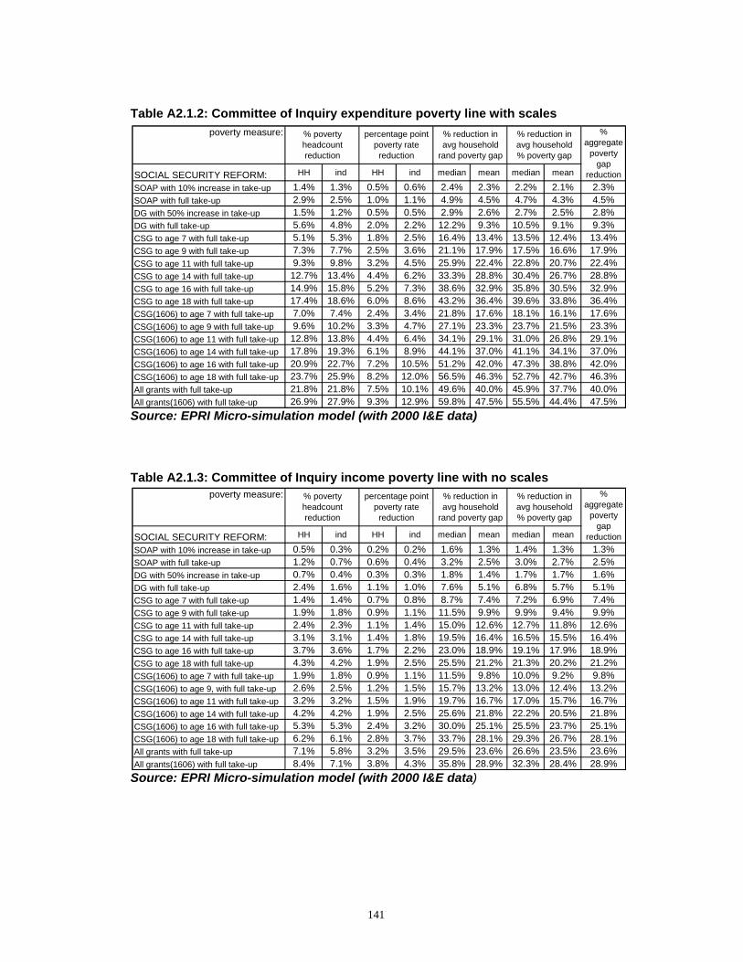
141
Table A2.1.2: Committee of Inquiry expenditure poverty line with scales
Source: EPRI Micro-simulation model (with 2000 I&E data) Table A2.1.3: Committee of Inquiry income poverty line with no scales
Source: EPRI Micro-simulation model (with 2000 I&E data)
poverty measure:
SOCIAL SECURITY REFORM: HH ind HH ind median mean median mean
SOAP with 10% increase in take-up 1.4% 1.3% 0.5% 0.6% 2.4% 2.3% 2.2% 2.1% 2.3%SOAP with full take-up 2.9% 2.5% 1.0% 1.1% 4.9% 4.5% 4.7% 4.3% 4.5%DG with 50% increase in take-up 1.5% 1.2% 0.5% 0.5% 2.9% 2.6% 2.7% 2.5% 2.8%DG with full take-up 5.6% 4.8% 2.0% 2.2% 12.2% 9.3% 10.5% 9.1% 9.3%CSG to age 7 with full take-up 5.1% 5.3% 1.8% 2.5% 16.4% 13.4% 13.5% 12.4% 13.4%CSG to age 9 with full take-up 7.3% 7.7% 2.5% 3.6% 21.1% 17.9% 17.5% 16.6% 17.9%CSG to age 11 with full take-up 9.3% 9.8% 3.2% 4.5% 25.9% 22.4% 22.8% 20.7% 22.4%CSG to age 14 with full take-up 12.7% 13.4% 4.4% 6.2% 33.3% 28.8% 30.4% 26.7% 28.8%CSG to age 16 with full take-up 14.9% 15.8% 5.2% 7.3% 38.6% 32.9% 35.8% 30.5% 32.9%CSG to age 18 with full take-up 17.4% 18.6% 6.0% 8.6% 43.2% 36.4% 39.6% 33.8% 36.4%CSG(1606) to age 7 with full take-up 7.0% 7.4% 2.4% 3.4% 21.8% 17.6% 18.1% 16.1% 17.6%CSG(1606) to age 9 with full take-up 9.6% 10.2% 3.3% 4.7% 27.1% 23.3% 23.7% 21.5% 23.3%CSG(1606) to age 11 with full take-up 12.8% 13.8% 4.4% 6.4% 34.1% 29.1% 31.0% 26.8% 29.1%CSG(1606) to age 14 with full take-up 17.8% 19.3% 6.1% 8.9% 44.1% 37.0% 41.1% 34.1% 37.0%CSG(1606) to age 16 with full take-up 20.9% 22.7% 7.2% 10.5% 51.2% 42.0% 47.3% 38.8% 42.0%CSG(1606) to age 18 with full take-up 23.7% 25.9% 8.2% 12.0% 56.5% 46.3% 52.7% 42.7% 46.3%All grants with full take-up 21.8% 21.8% 7.5% 10.1% 49.6% 40.0% 45.9% 37.7% 40.0%All grants(1606) with full take-up 26.9% 27.9% 9.3% 12.9% 59.8% 47.5% 55.5% 44.4% 47.5%
% aggregate
poverty gap
reduction
% reduction in avg household
rand poverty gap
% reduction in avg household % poverty gap
% poverty headcount reduction
percentage point poverty rate
reduction
poverty measure:
SOCIAL SECURITY REFORM: HH ind HH ind median mean median mean
SOAP with 10% increase in take-up 0.5% 0.3% 0.2% 0.2% 1.6% 1.3% 1.4% 1.3% 1.3%SOAP with full take-up 1.2% 0.7% 0.6% 0.4% 3.2% 2.5% 3.0% 2.7% 2.5%DG with 50% increase in take-up 0.7% 0.4% 0.3% 0.3% 1.8% 1.4% 1.7% 1.7% 1.6%DG with full take-up 2.4% 1.6% 1.1% 1.0% 7.6% 5.1% 6.8% 5.7% 5.1%CSG to age 7 with full take-up 1.4% 1.4% 0.7% 0.8% 8.7% 7.4% 7.2% 6.9% 7.4%CSG to age 9 with full take-up 1.9% 1.8% 0.9% 1.1% 11.5% 9.9% 9.9% 9.4% 9.9%CSG to age 11 with full take-up 2.4% 2.3% 1.1% 1.4% 15.0% 12.6% 12.7% 11.8% 12.6%CSG to age 14 with full take-up 3.1% 3.1% 1.4% 1.8% 19.5% 16.4% 16.5% 15.5% 16.4%CSG to age 16 with full take-up 3.7% 3.6% 1.7% 2.2% 23.0% 18.9% 19.1% 17.9% 18.9%CSG to age 18 with full take-up 4.3% 4.2% 1.9% 2.5% 25.5% 21.2% 21.3% 20.2% 21.2%CSG(1606) to age 7 with full take-up 1.9% 1.8% 0.9% 1.1% 11.5% 9.8% 10.0% 9.2% 9.8%CSG(1606) to age 9, with full take-up 2.6% 2.5% 1.2% 1.5% 15.7% 13.2% 13.0% 12.4% 13.2%CSG(1606) to age 11 with full take-up 3.2% 3.2% 1.5% 1.9% 19.7% 16.7% 17.0% 15.7% 16.7%CSG(1606) to age 14 with full take-up 4.2% 4.2% 1.9% 2.5% 25.6% 21.8% 22.2% 20.5% 21.8%CSG(1606) to age 16 with full take-up 5.3% 5.3% 2.4% 3.2% 30.0% 25.1% 25.5% 23.7% 25.1%CSG(1606) to age 18 with full take-up 6.2% 6.1% 2.8% 3.7% 33.7% 28.1% 29.3% 26.7% 28.1%All grants with full take-up 7.1% 5.8% 3.2% 3.5% 29.5% 23.6% 26.6% 23.5% 23.6%All grants(1606) with full take-up 8.4% 7.1% 3.8% 4.3% 35.8% 28.9% 32.3% 28.4% 28.9%
% poverty headcount reduction
percentage point poverty rate
reduction
% reduction in avg household
rand poverty gap
% reduction in avg household % poverty gap
% aggregate
poverty gap
reduction
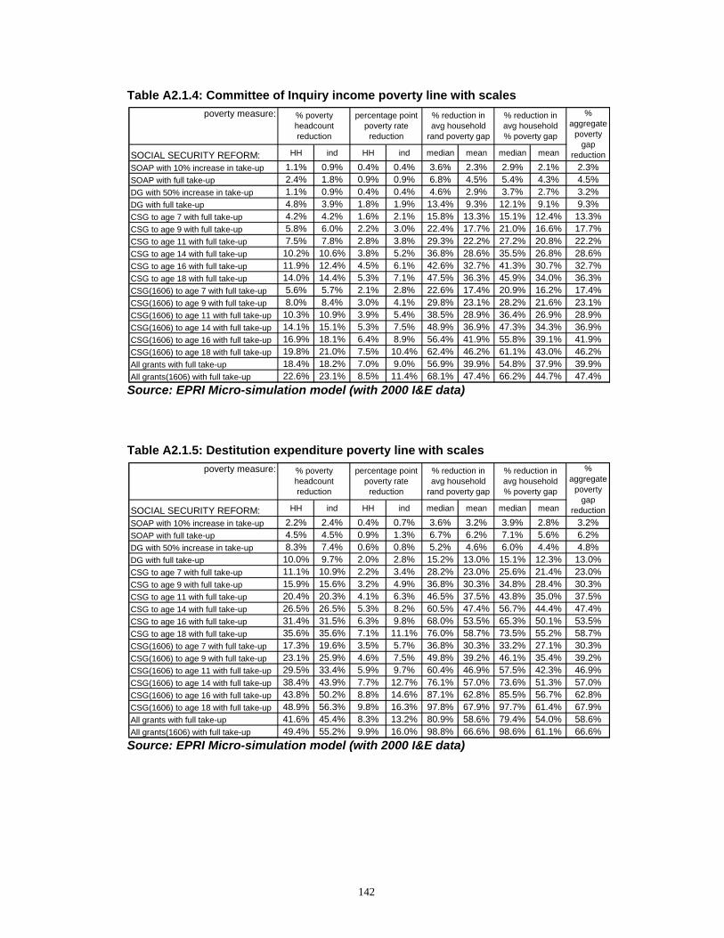
142
Table A2.1.4: Committee of Inquiry income poverty line with scales
Source: EPRI Micro-simulation model (with 2000 I&E data) Table A2.1.5: Destitution expenditure poverty line with scales
Source: EPRI Micro-simulation model (with 2000 I&E data)
poverty measure:
SOCIAL SECURITY REFORM: HH ind HH ind median mean median mean
SOAP with 10% increase in take-up 1.1% 0.9% 0.4% 0.4% 3.6% 2.3% 2.9% 2.1% 2.3%SOAP with full take-up 2.4% 1.8% 0.9% 0.9% 6.8% 4.5% 5.4% 4.3% 4.5%DG with 50% increase in take-up 1.1% 0.9% 0.4% 0.4% 4.6% 2.9% 3.7% 2.7% 3.2%DG with full take-up 4.8% 3.9% 1.8% 1.9% 13.4% 9.3% 12.1% 9.1% 9.3%CSG to age 7 with full take-up 4.2% 4.2% 1.6% 2.1% 15.8% 13.3% 15.1% 12.4% 13.3%CSG to age 9 with full take-up 5.8% 6.0% 2.2% 3.0% 22.4% 17.7% 21.0% 16.6% 17.7%CSG to age 11 with full take-up 7.5% 7.8% 2.8% 3.8% 29.3% 22.2% 27.2% 20.8% 22.2%CSG to age 14 with full take-up 10.2% 10.6% 3.8% 5.2% 36.8% 28.6% 35.5% 26.8% 28.6%CSG to age 16 with full take-up 11.9% 12.4% 4.5% 6.1% 42.6% 32.7% 41.3% 30.7% 32.7%CSG to age 18 with full take-up 14.0% 14.4% 5.3% 7.1% 47.5% 36.3% 45.9% 34.0% 36.3%CSG(1606) to age 7 with full take-up 5.6% 5.7% 2.1% 2.8% 22.6% 17.4% 20.9% 16.2% 17.4%CSG(1606) to age 9 with full take-up 8.0% 8.4% 3.0% 4.1% 29.8% 23.1% 28.2% 21.6% 23.1%CSG(1606) to age 11 with full take-up 10.3% 10.9% 3.9% 5.4% 38.5% 28.9% 36.4% 26.9% 28.9%CSG(1606) to age 14 with full take-up 14.1% 15.1% 5.3% 7.5% 48.9% 36.9% 47.3% 34.3% 36.9%CSG(1606) to age 16 with full take-up 16.9% 18.1% 6.4% 8.9% 56.4% 41.9% 55.8% 39.1% 41.9%CSG(1606) to age 18 with full take-up 19.8% 21.0% 7.5% 10.4% 62.4% 46.2% 61.1% 43.0% 46.2%All grants with full take-up 18.4% 18.2% 7.0% 9.0% 56.9% 39.9% 54.8% 37.9% 39.9%All grants(1606) with full take-up 22.6% 23.1% 8.5% 11.4% 68.1% 47.4% 66.2% 44.7% 47.4%
% reduction in avg household
rand poverty gap
% poverty headcount reduction
percentage point poverty rate
reduction
% reduction in avg household % poverty gap
% aggregate
poverty gap
reduction
poverty measure:
SOCIAL SECURITY REFORM: HH ind HH ind median mean median mean
SOAP with 10% increase in take-up 2.2% 2.4% 0.4% 0.7% 3.6% 3.2% 3.9% 2.8% 3.2%SOAP with full take-up 4.5% 4.5% 0.9% 1.3% 6.7% 6.2% 7.1% 5.6% 6.2%DG with 50% increase in take-up 8.3% 7.4% 0.6% 0.8% 5.2% 4.6% 6.0% 4.4% 4.8%DG with full take-up 10.0% 9.7% 2.0% 2.8% 15.2% 13.0% 15.1% 12.3% 13.0%CSG to age 7 with full take-up 11.1% 10.9% 2.2% 3.4% 28.2% 23.0% 25.6% 21.4% 23.0%CSG to age 9 with full take-up 15.9% 15.6% 3.2% 4.9% 36.8% 30.3% 34.8% 28.4% 30.3%CSG to age 11 with full take-up 20.4% 20.3% 4.1% 6.3% 46.5% 37.5% 43.8% 35.0% 37.5%CSG to age 14 with full take-up 26.5% 26.5% 5.3% 8.2% 60.5% 47.4% 56.7% 44.4% 47.4%CSG to age 16 with full take-up 31.4% 31.5% 6.3% 9.8% 68.0% 53.5% 65.3% 50.1% 53.5%CSG to age 18 with full take-up 35.6% 35.6% 7.1% 11.1% 76.0% 58.7% 73.5% 55.2% 58.7%CSG(1606) to age 7 with full take-up 17.3% 19.6% 3.5% 5.7% 36.8% 30.3% 33.2% 27.1% 30.3%CSG(1606) to age 9 with full take-up 23.1% 25.9% 4.6% 7.5% 49.8% 39.2% 46.1% 35.4% 39.2%CSG(1606) to age 11 with full take-up 29.5% 33.4% 5.9% 9.7% 60.4% 46.9% 57.5% 42.3% 46.9%CSG(1606) to age 14 with full take-up 38.4% 43.9% 7.7% 12.7% 76.1% 57.0% 73.6% 51.3% 57.0%CSG(1606) to age 16 with full take-up 43.8% 50.2% 8.8% 14.6% 87.1% 62.8% 85.5% 56.7% 62.8%CSG(1606) to age 18 with full take-up 48.9% 56.3% 9.8% 16.3% 97.8% 67.9% 97.7% 61.4% 67.9%All grants with full take-up 41.6% 45.4% 8.3% 13.2% 80.9% 58.6% 79.4% 54.0% 58.6%All grants(1606) with full take-up 49.4% 55.2% 9.9% 16.0% 98.8% 66.6% 98.6% 61.1% 66.6%
% reduction in avg household
rand poverty gap
% aggregate
poverty gap
reduction
% reduction in avg household % poverty gap
% poverty headcount reduction
percentage point poverty rate
reduction
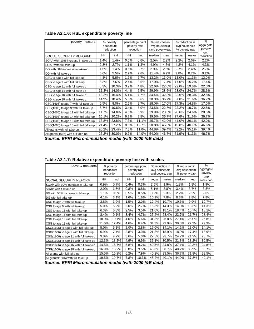
143
Table A2.1.6: HSL expenditure poverty line
Source: EPRI Micro-simulation model (with 2000 I&E data) Table A2.1.7: Relative expenditure poverty line with scales
Source: EPRI Micro-simulation model (with 2000 I&E data)
poverty measure:
SOCIAL SECURITY REFORM: HH ind HH ind median mean median mean
SOAP with 10% increase in take-up 1.4% 1.4% 0.5% 0.6% 2.5% 2.2% 2.2% 2.0% 2.2%SOAP with full take-up 2.8% 2.7% 1.1% 1.3% 4.9% 4.3% 4.3% 4.1% 4.3%DG with 50% increase in take-up 1.5% 1.4% 0.6% 0.7% 2.9% 2.6% 2.7% 2.4% 2.7%DG with full take-up 5.6% 5.5% 2.2% 2.6% 11.4% 9.2% 9.8% 8.7% 9.2%CSG to age 7 with full take-up 4.8% 5.8% 1.9% 2.7% 13.2% 13.0% 13.0% 11.3% 13.0%CSG to age 9 with full take-up 6.3% 7.6% 2.4% 3.6% 17.9% 17.4% 17.0% 15.2% 17.4%CSG to age 11 with full take-up 8.3% 10.3% 3.2% 4.8% 22.6% 22.0% 22.0% 19.0% 22.0%CSG to age 14 with full take-up 11.3% 14.0% 4.4% 6.5% 29.9% 28.6% 28.0% 24.7% 28.6%CSG to age 16 with full take-up 13.2% 16.4% 5.1% 7.7% 34.4% 32.8% 32.6% 28.3% 32.8%CSG to age 18 with full take-up 14.9% 18.4% 5.8% 8.6% 38.3% 36.7% 37.0% 31.6% 36.7%CSG(1606) to age 7 with full take-up 6.5% 8.0% 2.5% 3.7% 18.0% 17.0% 17.3% 14.8% 17.0%CSG(1606) to age 9 with full take-up 8.7% 10.8% 3.4% 5.0% 23.5% 22.8% 22.2% 19.7% 22.8%CSG(1606) to age 11 with full take-up 11.7% 14.8% 4.5% 6.9% 29.9% 28.5% 28.6% 24.6% 28.5%CSG(1606) to age 14 with full take-up 16.1% 20.2% 6.2% 9.5% 39.5% 36.7% 37.6% 31.6% 36.7%CSG(1606) to age 16 with full take-up 18.8% 23.8% 7.3% 11.1% 45.7% 42.0% 44.0% 36.1% 42.0%CSG(1606) to age 18 with full take-up 21.4% 27.2% 8.3% 12.7% 50.8% 46.6% 49.8% 40.1% 46.6%All grants with full take-up 20.2% 23.4% 7.8% 11.0% 44.8% 39.4% 42.2% 35.1% 39.4%All grants(1606) with full take-up 25.2% 30.0% 9.7% 14.0% 54.0% 46.7% 51.9% 41.3% 46.7%
% reduction in avg household
rand poverty gap
% poverty headcount reduction
percentage point poverty rate
reduction
% reduction in avg household % poverty gap
% aggregate
poverty gap
reduction
poverty measure:
SOCIAL SECURITY REFORM: HH ind HH ind median mean median mean
SOAP with 10% increase in take-up 0.9% 0.7% 0.4% 0.3% 2.5% 1.9% 1.8% 1.8% 1.9%SOAP with full take-up 2.0% 1.5% 0.8% 0.8% 5.1% 3.8% 3.4% 3.7% 3.8%DG with 50% increase in take-up 1.1% 0.9% 0.5% 0.5% 3.2% 2.3% 2.2% 2.2% 2.6%DG with full take-up 4.1% 3.1% 1.6% 1.6% 10.2% 7.8% 8.3% 7.8% 7.8%CSG to age 7 with full take-up 3.8% 3.9% 1.5% 2.0% 12.4% 10.7% 10.6% 9.9% 10.7%CSG to age 9 with full take-up 5.0% 5.2% 2.0% 2.7% 16.8% 14.3% 14.3% 13.3% 14.3%CSG to age 11 with full take-up 6.3% 6.8% 2.5% 3.5% 21.0% 18.1% 18.4% 16.7% 18.1%CSG to age 14 with full take-up 8.4% 9.1% 3.4% 4.7% 27.2% 23.4% 23.7% 21.7% 23.4%CSG to age 16 with full take-up 10.0% 10.7% 4.0% 5.6% 31.8% 26.8% 27.4% 25.0% 26.8%CSG to age 18 with full take-up 11.6% 12.4% 4.6% 6.4% 34.3% 29.9% 30.5% 27.9% 29.9%CSG(1606) to age 7 with full take-up 5.0% 5.3% 2.0% 2.8% 16.0% 14.1% 14.1% 13.0% 14.1%CSG(1606) to age 9 with full take-up 6.9% 7.4% 2.8% 3.9% 21.8% 18.9% 18.9% 17.4% 18.9%CSG(1606) to age 11 with full take-up 9.0% 9.7% 3.6% 5.0% 27.5% 23.7% 24.2% 21.9% 23.7%CSG(1606) to age 14 with full take-up 12.3% 13.2% 4.9% 6.9% 35.1% 30.5% 31.3% 28.2% 30.5%CSG(1606) to age 16 with full take-up 14.5% 15.7% 5.8% 8.2% 40.5% 34.8% 37.1% 32.3% 34.8%CSG(1606) to age 18 with full take-up 16.9% 18.2% 6.8% 9.5% 45.0% 38.7% 40.7% 35.9% 38.7%All grants with full take-up 15.5% 15.2% 6.2% 7.9% 40.2% 33.5% 36.7% 31.8% 33.5%All grants(1606) with full take-up 19.5% 19.7% 7.8% 10.3% 48.2% 40.1% 44.0% 37.8% 40.1%
% aggregate
poverty gap
reduction
% reduction in avg household
rand poverty gap
% poverty headcount reduction
percentage point poverty rate
reduction
% reduction in avg household % poverty gap

144
APPENDIX A2.2: Micro-simulation results from modelling policy scenarios Table A2.2.1.
Table A2.2.1 above shows the impact of the SOAP with 10% increase, analysed using the Committee of Inquiry expenditure poverty line with no scales. For example, the table indicates that 91,338 individuals are freed from poverty, reducing the poverty rate by 0.2 percentage points. The median rand poverty gap is reduced by 1.4% nationally, while the median percentage poverty gap falls by 1.4%. The aggregate rand poverty gap falls by 1.2% nationally.
SOAP with 10% increase in take-up, using Committee of Inquiry expenditure poverty line with no scales
households individuals # of new grants
% change since 2000 households individuals households individuals
National 1767591 4887482 25326696 170542 9.6% 26545 91338 0.5% 0.4%Western Cape 115210 252428 1317759 8359 7.3% 316 948 0.1% 0.1%Eastern Cape 359973 951191 4755398 32942 9.2% 5813 14929 0.6% 0.3%Northern Cape 30040 88744 388319 2600 8.7% 1005 2753 1.1% 0.7%Free State 93003 356495 1538747 8459 9.1% 1363 3478 0.4% 0.2%KwaZulu-Natal 358184 1047001 6074197 32751 9.1% 3455 9047 0.3% 0.1%Northwest 139114 376658 1878601 14017 10.1% 4141 16154 1.1% 0.9%Gauteng 304931 796871 4028132 39316 12.9% 7090 31433 0.9% 0.8%Mpumalanga 97852 305035 1656114 9003 9.2% 923 2981 0.3% 0.2%Limpopo 269284 713059 3689429 23095 8.6% 2439 9615 0.3% 0.3%
households individuals households individuals households individuals households individualsNational 44.3% 59.3% National 44.1% 59.1% 0.2% 0.2% 0.5% 0.4%Western Cape 23.6% 33.2% Western Cape 23.6% 33.2% 0.0% 0.0% 0.1% 0.1%Eastern Cape 65.9% 76.4% Eastern Cape 65.5% 76.1% 0.4% 0.2% 0.6% 0.3%Northern Cape 47.4% 59.5% Northern Cape 46.9% 59.1% 0.5% 0.4% 1.1% 0.7%Free State 50.6% 63.4% Free State 50.4% 63.3% 0.2% 0.1% 0.4% 0.2%KwaZulu-Natal 51.0% 68.0% KwaZulu-Natal 50.8% 67.9% 0.2% 0.1% 0.3% 0.1%Northwest 47.3% 64.1% Northwest 46.8% 63.5% 0.5% 0.6% 1.1% 0.9%Gauteng 25.8% 39.0% Gauteng 25.6% 38.7% 0.2% 0.3% 0.9% 0.8%Mpumalanga 46.8% 62.6% Mpumalanga 46.6% 62.5% 0.1% 0.1% 0.3% 0.2%Limpopo 69.2% 79.9% Limpopo 69.0% 79.7% 0.2% 0.2% 0.3% 0.3%
Median Mean Median Mean Median Mean Median MeanNational 860 1080 National 849 1067 12 13 1.4% 1.2%Western Cape 588 755 Western Cape 586 750 17 5 2.9% 0.6%Eastern Cape 997 1176 Eastern Cape 979 1161 17 16 1.7% 1.3%Northern Cape 704 898 Northern Cape 704 890 0 7 0.0% 0.8%Free State 826 967 Free State 817 956 9 11 1.1% 1.1%KwaZulu-Natal 995 1289 KwaZulu-Natal 985 1276 10 13 1.0% 1.0%Northwest 803 1038 Northwest 797 1025 6 14 0.7% 1.3%Gauteng 566 828 Gauteng 558 811 9 17 1.5% 2.0%Mpumalanga 853 1057 Mpumalanga 845 1048 8 9 0.9% 0.9%Limpopo 998 1154 Limpopo 988 1140 11 14 1.1% 1.2%
Median Mean Median Mean Median Mean Median MeanNational 50.5% 48.6% National 49.8% 48.0% 0.7% 0.6% 1.4% 1.3%Western Cape 34.6% 35.5% Western Cape 34.5% 35.3% 0.0% 0.2% 0.1% 0.5%Eastern Cape 58.1% 54.9% Eastern Cape 57.4% 54.0% 0.8% 0.9% 1.3% 1.6%Northern Cape 47.2% 47.2% Northern Cape 47.1% 46.8% 0.1% 0.4% 0.1% 0.9%Free State 56.4% 53.2% Free State 55.9% 52.6% 0.5% 0.6% 0.9% 1.1%KwaZulu-Natal 53.2% 50.8% KwaZulu-Natal 52.5% 50.2% 0.7% 0.6% 1.3% 1.1%Northwest 48.6% 48.3% Northwest 47.7% 47.6% 0.9% 0.7% 1.9% 1.4%Gauteng 37.7% 38.3% Gauteng 36.8% 37.6% 0.9% 0.7% 2.4% 1.8%Mpumalanga 46.3% 44.9% Mpumalanga 45.8% 44.5% 0.5% 0.4% 1.2% 0.9%Limpopo 55.6% 52.7% Limpopo 54.8% 52.1% 0.8% 0.6% 1.4% 1.2%
Statistics SA I&E 2000
Micro-simulation Rand difference % change
National 63368 62583 785 1.2%Western Cape 2288 2273 15 0.6%Eastern Cape 13429 13249 180 1.3%Northern Cape 956 948 8 0.8%Free State 4137 4091 47 1.1%KwaZulu-Natal 16203 16043 160 1.0%Northwest 4692 4631 61 1.3%Gauteng 7917 7757 160 2.0%Mpumalanga 3869 3835 35 0.9%Limpopo 9876 9757 119 1.2%
% change
Headcount poverty rates
# of new grants # freed from poverty As % of the poor in September 2000
Statistics SA I&E 2000 % point difference
Statistics SA I&E 2000 Micro-simulation model Rand differenceAverage household rand poverty gap
% change
% changeMicro-simulation model
Total rand poverty gap (R millions)
Statistics SA I&E 2000 Micro-simulation model
Micro-simulation modelStatistics SA I&E 2000
Poverty Headcount# grant
recipients
% point differenceAverage household percentage poverty gap
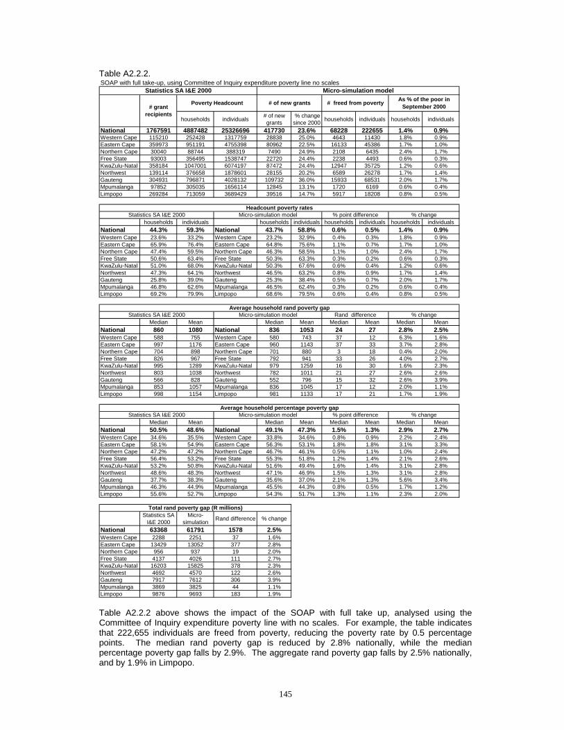
145
Table A2.2.2.
Table A2.2.2 above shows the impact of the SOAP with full take up, analysed using the Committee of Inquiry expenditure poverty line with no scales. For example, the table indicates that 222,655 individuals are freed from poverty, reducing the poverty rate by 0.5 percentage points. The median rand poverty gap is reduced by 2.8% nationally, while the median percentage poverty gap falls by 2.9%. The aggregate rand poverty gap falls by 2.5% nationally, and by 1.9% in Limpopo.
SOAP with full take-up, using Committee of Inquiry expenditure poverty line no scales
households individuals # of new grants
% change since 2000 households individuals households individuals
National 1767591 4887482 25326696 417730 23.6% 68228 222655 1.4% 0.9%Western Cape 115210 252428 1317759 28838 25.0% 4643 11430 1.8% 0.9%Eastern Cape 359973 951191 4755398 80962 22.5% 16133 45386 1.7% 1.0%Northern Cape 30040 88744 388319 7490 24.9% 2108 6435 2.4% 1.7%Free State 93003 356495 1538747 22720 24.4% 2238 4493 0.6% 0.3%KwaZulu-Natal 358184 1047001 6074197 87472 24.4% 12947 35725 1.2% 0.6%Northwest 139114 376658 1878601 28155 20.2% 6589 26278 1.7% 1.4%Gauteng 304931 796871 4028132 109732 36.0% 15933 68531 2.0% 1.7%Mpumalanga 97852 305035 1656114 12845 13.1% 1720 6169 0.6% 0.4%Limpopo 269284 713059 3689429 39516 14.7% 5917 18208 0.8% 0.5%
households individuals households individuals households individuals households individualsNational 44.3% 59.3% National 43.7% 58.8% 0.6% 0.5% 1.4% 0.9%Western Cape 23.6% 33.2% Western Cape 23.2% 32.9% 0.4% 0.3% 1.8% 0.9%Eastern Cape 65.9% 76.4% Eastern Cape 64.8% 75.6% 1.1% 0.7% 1.7% 1.0%Northern Cape 47.4% 59.5% Northern Cape 46.3% 58.5% 1.1% 1.0% 2.4% 1.7%Free State 50.6% 63.4% Free State 50.3% 63.3% 0.3% 0.2% 0.6% 0.3%KwaZulu-Natal 51.0% 68.0% KwaZulu-Natal 50.3% 67.6% 0.6% 0.4% 1.2% 0.6%Northwest 47.3% 64.1% Northwest 46.5% 63.2% 0.8% 0.9% 1.7% 1.4%Gauteng 25.8% 39.0% Gauteng 25.3% 38.4% 0.5% 0.7% 2.0% 1.7%Mpumalanga 46.8% 62.6% Mpumalanga 46.5% 62.4% 0.3% 0.2% 0.6% 0.4%Limpopo 69.2% 79.9% Limpopo 68.6% 79.5% 0.6% 0.4% 0.8% 0.5%
Median Mean Median Mean Median Mean Median MeanNational 860 1080 National 836 1053 24 27 2.8% 2.5%Western Cape 588 755 Western Cape 580 743 37 12 6.3% 1.6%Eastern Cape 997 1176 Eastern Cape 960 1143 37 33 3.7% 2.8%Northern Cape 704 898 Northern Cape 701 880 3 18 0.4% 2.0%Free State 826 967 Free State 792 941 33 26 4.0% 2.7%KwaZulu-Natal 995 1289 KwaZulu-Natal 979 1259 16 30 1.6% 2.3%Northwest 803 1038 Northwest 782 1011 21 27 2.6% 2.6%Gauteng 566 828 Gauteng 552 796 15 32 2.6% 3.9%Mpumalanga 853 1057 Mpumalanga 836 1045 17 12 2.0% 1.1%Limpopo 998 1154 Limpopo 981 1133 17 21 1.7% 1.9%
Median Mean Median Mean Median Mean Median MeanNational 50.5% 48.6% National 49.1% 47.3% 1.5% 1.3% 2.9% 2.7%Western Cape 34.6% 35.5% Western Cape 33.8% 34.6% 0.8% 0.9% 2.2% 2.4%Eastern Cape 58.1% 54.9% Eastern Cape 56.3% 53.1% 1.8% 1.8% 3.1% 3.3%Northern Cape 47.2% 47.2% Northern Cape 46.7% 46.1% 0.5% 1.1% 1.0% 2.4%Free State 56.4% 53.2% Free State 55.3% 51.8% 1.2% 1.4% 2.1% 2.6%KwaZulu-Natal 53.2% 50.8% KwaZulu-Natal 51.6% 49.4% 1.6% 1.4% 3.1% 2.8%Northwest 48.6% 48.3% Northwest 47.1% 46.9% 1.5% 1.3% 3.1% 2.8%Gauteng 37.7% 38.3% Gauteng 35.6% 37.0% 2.1% 1.3% 5.6% 3.4%Mpumalanga 46.3% 44.9% Mpumalanga 45.5% 44.3% 0.8% 0.5% 1.7% 1.2%Limpopo 55.6% 52.7% Limpopo 54.3% 51.7% 1.3% 1.1% 2.3% 2.0%
Statistics SA I&E 2000
Micro-simulation Rand difference % change
National 63368 61791 1578 2.5%Western Cape 2288 2251 37 1.6%Eastern Cape 13429 13052 377 2.8%Northern Cape 956 937 19 2.0%Free State 4137 4026 111 2.7%KwaZulu-Natal 16203 15825 378 2.3%Northwest 4692 4570 122 2.6%Gauteng 7917 7612 306 3.9%Mpumalanga 3869 3825 44 1.1%Limpopo 9876 9693 183 1.9%
Total rand poverty gap (R millions)
Statistics SA I&E 2000 Micro-simulation model
Micro-simulation modelStatistics SA I&E 2000
Poverty Headcount# grant
recipients
% point differenceAverage household percentage poverty gap
Average household rand poverty gap% change
% changeMicro-simulation model
% change
Headcount poverty rates
# of new grants # freed from poverty As % of the poor in September 2000
Statistics SA I&E 2000 % point difference
Statistics SA I&E 2000 Micro-simulation model Rand difference
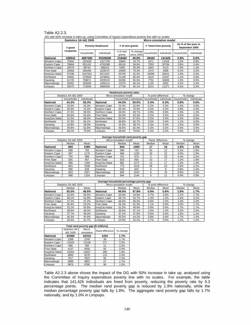
146
Table A2.2.3.
Table A2.2.3 above shows the impact of the DG with 50% increase in take up, analysed using the Committee of Inquiry expenditure poverty line with no scales. For example, the table indicates that 141,426 individuals are freed from poverty, reducing the poverty rate by 0.3 percentage points. The median rand poverty gap is reduced by 1.9% nationally, while the median percentage poverty gap falls by 1.8%. The aggregate rand poverty gap falls by 1.7% nationally, and by 1.0% in Limpopo.
DG with 50% increase in take-up, using Committee of Inquiry expenditure poverty line with no scales
households individuals # of new grants
% change since 2000 households individuals households individuals
National 438542 4887482 25326696 218460 49.8% 39442 141426 0.8% 0.6%Western Cape 70442 252428 1317759 13843 19.7% 2471 11016 1.0% 0.8%Eastern Cape 78664 951191 4755398 46316 58.9% 7550 20794 0.8% 0.4%Northern Cape 20076 88744 388319 5280 26.3% 1643 5123 1.9% 1.3%Free State 20069 356495 1538747 15909 79.3% 1574 4096 0.4% 0.3%KwaZulu-Natal 97038 1047001 6074197 50709 52.3% 10095 36451 1.0% 0.6%Northwest 34942 376658 1878601 21106 60.4% 4019 12037 1.1% 0.6%Gauteng 61745 796871 4028132 34265 55.5% 7752 34806 1.0% 0.9%Mpumalanga 20091 305035 1656114 13276 66.1% 1125 6032 0.4% 0.4%Limpopo 35475 713059 3689429 17756 50.1% 3213 11071 0.5% 0.3%
households individuals households individuals households individuals households individualsNational 44.3% 59.3% National 44.0% 59.0% 0.4% 0.3% 0.8% 0.6%Western Cape 23.6% 33.2% Western Cape 23.4% 32.9% 0.2% 0.3% 1.0% 0.8%Eastern Cape 65.9% 76.4% Eastern Cape 65.4% 76.0% 0.5% 0.3% 0.8% 0.4%Northern Cape 47.4% 59.5% Northern Cape 46.5% 58.7% 0.9% 0.8% 1.9% 1.3%Free State 50.6% 63.4% Free State 50.4% 63.3% 0.2% 0.2% 0.4% 0.3%KwaZulu-Natal 51.0% 68.0% KwaZulu-Natal 50.5% 67.6% 0.5% 0.4% 1.0% 0.6%Northwest 47.3% 64.1% Northwest 46.8% 63.7% 0.5% 0.4% 1.1% 0.6%Gauteng 25.8% 39.0% Gauteng 25.5% 38.7% 0.3% 0.3% 1.0% 0.9%Mpumalanga 46.8% 62.6% Mpumalanga 46.6% 62.4% 0.2% 0.2% 0.4% 0.4%Limpopo 69.2% 79.9% Limpopo 68.9% 79.6% 0.3% 0.2% 0.5% 0.3%
Median Mean Median Mean Median Mean Median MeanNational 860 1080 National 844 1065 17 16 1.9% 1.5%Western Cape 588 755 Western Cape 580 743 30 12 5.1% 1.6%Eastern Cape 997 1176 Eastern Cape 966 1155 30 22 3.0% 1.9%Northern Cape 704 898 Northern Cape 701 878 3 20 0.4% 2.2%Free State 826 967 Free State 816 950 10 17 1.2% 1.8%KwaZulu-Natal 995 1289 KwaZulu-Natal 982 1272 13 17 1.3% 1.3%Northwest 803 1038 Northwest 775 1015 28 23 3.5% 2.2%Gauteng 566 828 Gauteng 562 820 5 8 0.8% 1.0%Mpumalanga 853 1057 Mpumalanga 845 1042 8 15 0.9% 1.4%Limpopo 998 1154 Limpopo 994 1144 4 11 0.4% 0.9%
Median Mean Median Mean Median Mean Median MeanNational 50.5% 48.6% National 49.6% 47.8% 0.9% 0.8% 1.8% 1.7%Western Cape 34.6% 35.5% Western Cape 33.9% 34.9% 0.7% 0.6% 2.1% 1.7%Eastern Cape 58.1% 54.9% Eastern Cape 56.7% 53.7% 1.4% 1.2% 2.4% 2.2%Northern Cape 47.2% 47.2% Northern Cape 46.6% 46.2% 0.6% 1.0% 1.3% 2.2%Free State 56.4% 53.2% Free State 55.3% 52.3% 1.1% 0.9% 2.0% 1.7%KwaZulu-Natal 53.2% 50.8% KwaZulu-Natal 52.3% 49.9% 0.9% 0.9% 1.7% 1.7%Northwest 48.6% 48.3% Northwest 46.9% 47.1% 1.6% 1.2% 3.3% 2.5%Gauteng 37.7% 38.3% Gauteng 37.1% 37.9% 0.6% 0.4% 1.5% 1.1%Mpumalanga 46.3% 44.9% Mpumalanga 45.5% 44.2% 0.8% 0.6% 1.7% 1.4%Limpopo 55.6% 52.7% Limpopo 54.9% 52.2% 0.7% 0.6% 1.2% 1.0%
Statistics SA I&E 2000
Micro-simulation Rand difference % change
National 63368 62316 1052 1.7%Western Cape 2288 2249 39 1.7%Eastern Cape 13429 13158 271 2.0%Northern Cape 956 935 21 2.2%Free State 4137 4056 82 2.0%KwaZulu-Natal 16203 15937 266 1.6%Northwest 4692 4578 115 2.4%Gauteng 7917 7823 95 1.2%Mpumalanga 3869 3802 67 1.7%Limpopo 9876 9780 96 1.0%
% change
Headcount poverty rates
# of new grants # freed from poverty As % of the poor in September 2000
Statistics SA I&E 2000 % point difference
Statistics SA I&E 2000 Micro-simulation model Rand differenceAverage household rand poverty gap
% change
% changeMicro-simulation model
Total rand poverty gap (R millions)
Statistics SA I&E 2000 Micro-simulation model
Micro-simulation modelStatistics SA I&E 2000
Poverty Headcount# grant
recipients
% point differenceAverage household percentage poverty gap

147
Table A2.2.4.
Table A2.2.4 above shows the impact of the DG with full take up, analysed using the Committee of Inquiry expenditure poverty line with no scales. For example, the table indicates that 448,199 individuals are freed from poverty, reducing the poverty rate by 1.0 percentage points. The median rand poverty gap is reduced by 6.5% nationally, while the median percentage poverty gap falls by 6.2%. The aggregate rand poverty gap falls by 5.1% nationally, and by 3.8% in Limpopo.
DG with full take-up, using Committee of Inquiry expenditure poverty line with no scales
households individuals # of new grants
% change since 2000 households individuals households individuals
National 438542 4887482 25326696 780318 177.9% 133791 448199 2.7% 1.8%Western Cape 70442 252428 1317759 55546 78.9% 10804 44220 4.3% 3.4%Eastern Cape 78664 951191 4755398 150466 191.3% 28713 78229 3.0% 1.6%Northern Cape 20076 88744 388319 22818 113.7% 4336 12856 4.9% 3.3%Free State 20069 356495 1538747 54619 272.2% 7975 24773 2.2% 1.6%KwaZulu-Natal 97038 1047001 6074197 158093 162.9% 20406 72912 1.9% 1.2%Northwest 34942 376658 1878601 74196 212.3% 16098 49617 4.3% 2.6%Gauteng 61745 796871 4028132 136145 220.5% 26701 103387 3.4% 2.6%Mpumalanga 20091 305035 1656114 52758 262.6% 8711 33735 2.9% 2.0%Limpopo 35475 713059 3689429 75677 213.3% 10047 28470 1.4% 0.8%
households individuals households individuals households individuals households individualsNational 44.3% 59.3% National 43.1% 58.2% 1.2% 1.0% 2.7% 1.8%Western Cape 23.6% 33.2% Western Cape 22.6% 32.1% 1.0% 1.1% 4.3% 3.4%Eastern Cape 65.9% 76.4% Eastern Cape 63.9% 75.1% 2.0% 1.3% 3.0% 1.6%Northern Cape 47.4% 59.5% Northern Cape 45.1% 57.5% 2.3% 2.0% 4.9% 3.3%Free State 50.6% 63.4% Free State 49.5% 62.4% 1.1% 1.0% 2.2% 1.6%KwaZulu-Natal 51.0% 68.0% KwaZulu-Natal 50.0% 67.1% 1.0% 0.8% 1.9% 1.2%Northwest 47.3% 64.1% Northwest 45.3% 62.4% 2.0% 1.7% 4.3% 2.6%Gauteng 25.8% 39.0% Gauteng 24.9% 38.0% 0.9% 1.0% 3.4% 2.6%Mpumalanga 46.8% 62.6% Mpumalanga 45.4% 61.4% 1.3% 1.3% 2.9% 2.0%Limpopo 69.2% 79.9% Limpopo 68.2% 79.3% 1.0% 0.6% 1.4% 0.8%
Median Mean Median Mean Median Mean Median MeanNational 860 1080 National 804 1026 56 55 6.5% 5.1%Western Cape 588 755 Western Cape 557 712 65 43 11.1% 5.7%Eastern Cape 997 1176 Eastern Cape 931 1113 65 64 6.5% 5.4%Northern Cape 704 898 Northern Cape 625 815 79 83 11.3% 9.2%Free State 826 967 Free State 774 915 52 52 6.3% 5.4%KwaZulu-Natal 995 1289 KwaZulu-Natal 943 1234 52 54 5.3% 4.2%Northwest 803 1038 Northwest 724 958 79 80 9.8% 7.8%Gauteng 566 828 Gauteng 540 787 26 41 4.6% 5.0%Mpumalanga 853 1057 Mpumalanga 809 994 45 63 5.2% 6.0%Limpopo 998 1154 Limpopo 954 1111 44 43 4.4% 3.8%
Median Mean Median Mean Median Mean Median MeanNational 50.5% 48.6% National 47.4% 45.8% 3.2% 2.8% 6.2% 5.7%Western Cape 34.6% 35.5% Western Cape 32.2% 33.4% 2.4% 2.2% 6.9% 6.1%Eastern Cape 58.1% 54.9% Eastern Cape 55.0% 51.4% 3.2% 3.4% 5.5% 6.3%Northern Cape 47.2% 47.2% Northern Cape 43.1% 42.8% 4.1% 4.4% 8.7% 9.2%Free State 56.4% 53.2% Free State 53.7% 50.3% 2.7% 2.9% 4.9% 5.4%KwaZulu-Natal 53.2% 50.8% KwaZulu-Natal 50.1% 48.3% 3.1% 2.5% 5.8% 4.9%Northwest 48.6% 48.3% Northwest 44.4% 44.2% 4.2% 4.1% 8.6% 8.5%Gauteng 37.7% 38.3% Gauteng 34.8% 36.2% 2.9% 2.1% 7.6% 5.5%Mpumalanga 46.3% 44.9% Mpumalanga 42.7% 42.0% 3.6% 2.9% 7.9% 6.4%Limpopo 55.6% 52.7% Limpopo 53.1% 50.4% 2.5% 2.4% 4.6% 4.5%
Statistics SA I&E 2000
Micro-simulation Rand difference % change
National 63368 60158 3211 5.1%Western Cape 2288 2158 130 5.7%Eastern Cape 13429 12702 727 5.4%Northern Cape 956 868 88 9.2%Free State 4137 3915 222 5.4%KwaZulu-Natal 16203 15519 684 4.2%Northwest 4692 4329 364 7.8%Gauteng 7917 7524 393 5.0%Mpumalanga 3869 3638 231 6.0%Limpopo 9876 9505 371 3.8%
% change
Headcount poverty rates
# of new grants # freed from poverty As % of the poor in September 2000
Statistics SA I&E 2000 % point difference
Statistics SA I&E 2000 Micro-simulation model Rand differenceAverage household rand poverty gap
% change
% changeMicro-simulation model
Total rand poverty gap (R millions)
Statistics SA I&E 2000 Micro-simulation model
Micro-simulation modelStatistics SA I&E 2000
Poverty Headcount# grant
recipients
% point differenceAverage household percentage poverty gap

148
Table A2.2.5.
Table A2.2.5 above shows the impact of the CSG at an annual level of R1200 in 2000, with full take up to the age 7, analysed using the Committee of Inquiry expenditure poverty line with no scales. For example, the table indicates that 444,566 individuals are freed from poverty, reducing the poverty rate by 1.0 percentage points. The median rand poverty gap is reduced by 8.6% nationally, while the median percentage poverty gap falls by 6.8%. The aggregate rand poverty gap falls by 7.5% nationally, and by 7.7% in Limpopo.
CSG to age 7 with full take-up, using Committee of Inquiry expenditure poverty line no scales
households individuals # of new grants
% change since 2000 households individuals households individuals
National 463699 4887482 25326696 4026590 868.4% 91683 444566 1.9% 1.8%Western Cape 59407 252428 1317759 210409 354.2% 13615 75413 5.4% 5.7%Eastern Cape 63038 951191 4755398 769172 1220.2% 6687 29527 0.7% 0.6%Northern Cape 19734 88744 388319 60684 307.5% 1575 5320 1.8% 1.4%Free State 18573 356495 1538747 202617 1090.9% 2841 10125 0.8% 0.7%KwaZulu-Natal 70660 1047001 6074197 1042611 1475.5% 11702 54235 1.1% 0.9%Northwest 34341 376658 1878601 274279 798.7% 6511 31279 1.7% 1.7%Gauteng 107493 796871 4028132 574022 534.0% 37137 182037 4.7% 4.5%Mpumalanga 43704 305035 1656114 250306 572.7% 5645 22685 1.9% 1.4%Limpopo 46749 713059 3689429 642490 1374.3% 5970 33945 0.8% 0.9%
households individuals households individuals households individuals households individualsNational 44.3% 59.3% National 43.5% 58.2% 0.8% 1.0% 1.9% 1.8%Western Cape 23.6% 33.2% Western Cape 22.3% 31.3% 1.3% 1.9% 5.4% 5.7%Eastern Cape 65.9% 76.4% Eastern Cape 65.4% 75.9% 0.5% 0.5% 0.7% 0.6%Northern Cape 47.4% 59.5% Northern Cape 46.6% 58.7% 0.8% 0.8% 1.8% 1.4%Free State 50.6% 63.4% Free State 50.2% 63.0% 0.4% 0.4% 0.8% 0.7%KwaZulu-Natal 51.0% 68.0% KwaZulu-Natal 50.4% 67.3% 0.6% 0.6% 1.1% 0.9%Northwest 47.3% 64.1% Northwest 46.5% 63.0% 0.8% 1.1% 1.7% 1.7%Gauteng 25.8% 39.0% Gauteng 24.6% 37.3% 1.2% 1.8% 4.7% 4.5%Mpumalanga 46.8% 62.6% Mpumalanga 45.9% 61.8% 0.9% 0.9% 1.9% 1.4%Limpopo 69.2% 79.9% Limpopo 68.6% 79.1% 0.6% 0.7% 0.8% 0.9%
Median Mean Median Mean Median Mean Median MeanNational 860 1080 National 786 999 74 81 8.6% 7.5%Western Cape 588 755 Western Cape 517 676 76 79 13.0% 10.5%Eastern Cape 997 1176 Eastern Cape 920 1096 76 80 7.7% 6.8%Northern Cape 704 898 Northern Cape 642 831 62 67 8.8% 7.5%Free State 826 967 Free State 761 911 65 56 7.8% 5.8%KwaZulu-Natal 995 1289 KwaZulu-Natal 919 1190 77 99 7.7% 7.7%Northwest 803 1038 Northwest 733 966 70 72 8.7% 6.9%Gauteng 566 828 Gauteng 512 759 54 69 9.6% 8.3%Mpumalanga 853 1057 Mpumalanga 782 976 72 81 8.4% 7.6%Limpopo 998 1154 Limpopo 937 1065 61 89 6.1% 7.7%
Median Mean Median Mean Median Mean Median MeanNational 50.5% 48.6% National 47.1% 45.2% 3.4% 3.4% 6.8% 7.0%Western Cape 34.6% 35.5% Western Cape 30.4% 31.8% 4.2% 3.7% 12.1% 10.4%Eastern Cape 58.1% 54.9% Eastern Cape 54.5% 51.5% 3.7% 3.4% 6.3% 6.3%Northern Cape 47.2% 47.2% Northern Cape 43.9% 44.0% 3.3% 3.2% 6.9% 6.8%Free State 56.4% 53.2% Free State 53.0% 50.3% 3.5% 2.8% 6.2% 5.3%KwaZulu-Natal 53.2% 50.8% KwaZulu-Natal 49.1% 47.1% 4.1% 3.7% 7.7% 7.3%Northwest 48.6% 48.3% Northwest 44.9% 45.3% 3.6% 3.0% 7.5% 6.2%Gauteng 37.7% 38.3% Gauteng 34.2% 35.2% 3.5% 3.1% 9.4% 8.2%Mpumalanga 46.3% 44.9% Mpumalanga 42.7% 41.5% 3.6% 3.4% 7.9% 7.5%Limpopo 55.6% 52.7% Limpopo 51.9% 49.0% 3.8% 3.8% 6.8% 7.1%
Statistics SA I&E 2000
Micro-simulation Rand difference % change
National 63368 58618 4750 7.5%Western Cape 2288 2048 239 10.5%Eastern Cape 13429 12511 917 6.8%Northern Cape 956 885 71 7.5%Free State 4137 3897 241 5.8%KwaZulu-Natal 16203 14961 1242 7.7%Northwest 4692 4368 324 6.9%Gauteng 7917 7262 655 8.3%Mpumalanga 3869 3574 295 7.6%Limpopo 9876 9112 764 7.7%
Total rand poverty gap (R millions)
Statistics SA I&E 2000 Micro-simulation model
Micro-simulation modelStatistics SA I&E 2000
Poverty Headcount# grant
recipients
% point differenceAverage household percentage poverty gap
Average household rand poverty gap% change
% changeMicro-simulation model
% change
Headcount poverty rates
# of new grants # freed from poverty As % of the poor in September 2000
Statistics SA I&E 2000 % point difference
Statistics SA I&E 2000 Micro-simulation model Rand difference

149
Table A2.2.6.
Table A2.2.6 above shows the impact of the CSG at an annual level of R1200 in 2000, with full take up to the age 9, analysed using the Committee of Inquiry expenditure poverty line with no scales. For example, the table indicates that 624,262 individuals are freed from poverty, reducing the poverty rate by 1.5 percentage points. The median rand poverty gap is reduced by 11.1% nationally, while the median percentage poverty gap falls by 9.1%. The aggregate rand poverty gap falls by 10.1% nationally, and by 10.3% in Limpopo.
CSG to age 9 with full take-up, using Committee of Inquiry expenditure poverty line no scales
households individuals # of new grants
% change since 2000 households individuals households individuals
National 463699 4887482 25326696 5413470 1167.5% 124703 624262 2.6% 2.5%Western Cape 59407 252428 1317759 274483 462.0% 15551 87513 6.2% 6.6%Eastern Cape 63038 951191 4755398 1045120 1657.9% 11160 48705 1.2% 1.0%Northern Cape 19734 88744 388319 77530 392.9% 2563 8840 2.9% 2.3%Free State 18573 356495 1538747 278621 1500.1% 4161 18157 1.2% 1.2%KwaZulu-Natal 70660 1047001 6074197 1403055 1985.6% 15216 73066 1.5% 1.2%Northwest 34341 376658 1878601 372722 1085.4% 10084 47984 2.7% 2.6%Gauteng 107493 796871 4028132 755032 702.4% 47156 248945 5.9% 6.2%Mpumalanga 43704 305035 1656114 346442 792.7% 7401 30952 2.4% 1.9%Limpopo 46749 713059 3689429 860465 1840.6% 11411 60100 1.6% 1.6%
households individuals households individuals households individuals households individualsNational 44.3% 59.3% National 43.2% 57.8% 1.1% 1.5% 2.6% 2.5%Western Cape 23.6% 33.2% Western Cape 22.2% 31.0% 1.5% 2.2% 6.2% 6.6%Eastern Cape 65.9% 76.4% Eastern Cape 65.1% 75.6% 0.8% 0.8% 1.2% 1.0%Northern Cape 47.4% 59.5% Northern Cape 46.0% 58.1% 1.4% 1.4% 2.9% 2.3%Free State 50.6% 63.4% Free State 50.0% 62.7% 0.6% 0.7% 1.2% 1.2%KwaZulu-Natal 51.0% 68.0% KwaZulu-Natal 50.2% 67.1% 0.8% 0.8% 1.5% 1.2%Northwest 47.3% 64.1% Northwest 46.1% 62.4% 1.3% 1.6% 2.7% 2.6%Gauteng 25.8% 39.0% Gauteng 24.3% 36.6% 1.5% 2.4% 5.9% 6.2%Mpumalanga 46.8% 62.6% Mpumalanga 45.6% 61.5% 1.1% 1.2% 2.4% 1.9%Limpopo 69.2% 79.9% Limpopo 68.1% 78.6% 1.1% 1.3% 1.6% 1.6%
Median Mean Median Mean Median Mean Median MeanNational 860 1080 National 765 972 95 109 11.1% 10.1%Western Cape 588 755 Western Cape 489 653 97 103 16.6% 13.6%Eastern Cape 997 1176 Eastern Cape 899 1067 97 109 9.8% 9.3%Northern Cape 704 898 Northern Cape 613 812 91 85 13.0% 9.5%Free State 826 967 Free State 747 890 79 77 9.5% 8.0%KwaZulu-Natal 995 1289 KwaZulu-Natal 902 1156 94 133 9.4% 10.3%Northwest 803 1038 Northwest 718 941 85 97 10.6% 9.3%Gauteng 566 828 Gauteng 489 738 77 90 13.7% 10.8%Mpumalanga 853 1057 Mpumalanga 745 946 108 111 12.6% 10.5%Limpopo 998 1154 Limpopo 892 1035 106 119 10.6% 10.3%
Median Mean Median Mean Median Mean Median MeanNational 50.5% 48.6% National 45.9% 44.0% 4.6% 4.6% 9.1% 9.5%Western Cape 34.6% 35.5% Western Cape 29.6% 30.8% 5.0% 4.7% 14.5% 13.2%Eastern Cape 58.1% 54.9% Eastern Cape 52.9% 50.2% 5.3% 4.7% 9.1% 8.5%Northern Cape 47.2% 47.2% Northern Cape 43.3% 43.1% 3.9% 4.1% 8.3% 8.6%Free State 56.4% 53.2% Free State 51.8% 49.3% 4.7% 3.9% 8.2% 7.4%KwaZulu-Natal 53.2% 50.8% KwaZulu-Natal 48.2% 45.8% 5.0% 5.0% 9.4% 9.9%Northwest 48.6% 48.3% Northwest 43.9% 44.2% 4.6% 4.1% 9.5% 8.5%Gauteng 37.7% 38.3% Gauteng 33.0% 34.2% 4.7% 4.1% 12.5% 10.6%Mpumalanga 46.3% 44.9% Mpumalanga 41.2% 40.2% 5.1% 4.7% 11.1% 10.4%Limpopo 55.6% 52.7% Limpopo 50.5% 47.7% 5.2% 5.1% 9.3% 9.6%
Statistics SA I&E 2000
Micro-simulation Rand difference % change
National 63368 56994 6374 10.1%Western Cape 2288 1977 311 13.6%Eastern Cape 13429 12183 1246 9.3%Northern Cape 956 865 91 9.5%Free State 4137 3807 331 8.0%KwaZulu-Natal 16203 14532 1671 10.3%Northwest 4692 4254 439 9.3%Gauteng 7917 7060 858 10.8%Mpumalanga 3869 3462 408 10.5%Limpopo 9876 8855 1021 10.3%
Total rand poverty gap (R millions)
Statistics SA I&E 2000 Micro-simulation model
Micro-simulation modelStatistics SA I&E 2000
Poverty Headcount# grant
recipients
% point differenceAverage household percentage poverty gap
Average household rand poverty gap% change
% changeMicro-simulation model
% change
Headcount poverty rates
# of new grants # freed from poverty As % of the poor in September 2000
Statistics SA I&E 2000 % point difference
Statistics SA I&E 2000 Micro-simulation model Rand difference
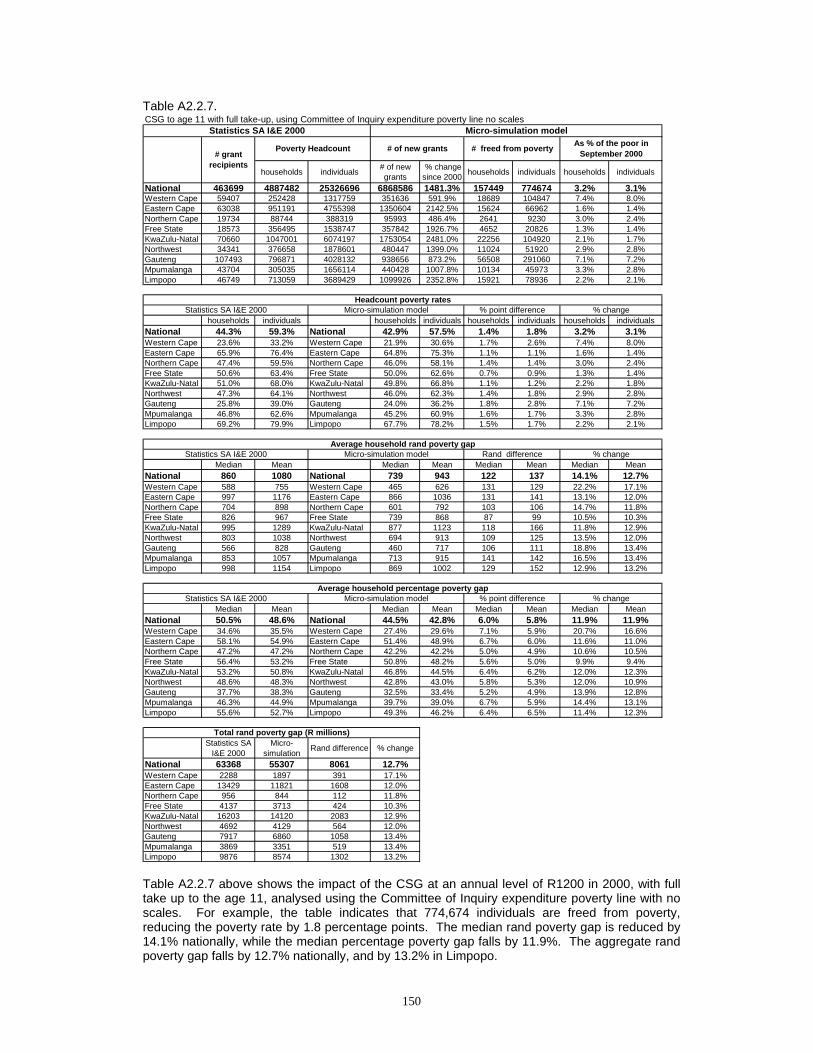
150
Table A2.2.7.
Table A2.2.7 above shows the impact of the CSG at an annual level of R1200 in 2000, with full take up to the age 11, analysed using the Committee of Inquiry expenditure poverty line with no scales. For example, the table indicates that 774,674 individuals are freed from poverty, reducing the poverty rate by 1.8 percentage points. The median rand poverty gap is reduced by 14.1% nationally, while the median percentage poverty gap falls by 11.9%. The aggregate rand poverty gap falls by 12.7% nationally, and by 13.2% in Limpopo.
CSG to age 11 with full take-up, using Committee of Inquiry expenditure poverty line no scales
households individuals # of new grants
% change since 2000 households individuals households individuals
National 463699 4887482 25326696 6868586 1481.3% 157449 774674 3.2% 3.1%Western Cape 59407 252428 1317759 351636 591.9% 18689 104847 7.4% 8.0%Eastern Cape 63038 951191 4755398 1350604 2142.5% 15624 66962 1.6% 1.4%Northern Cape 19734 88744 388319 95993 486.4% 2641 9230 3.0% 2.4%Free State 18573 356495 1538747 357842 1926.7% 4652 20826 1.3% 1.4%KwaZulu-Natal 70660 1047001 6074197 1753054 2481.0% 22256 104920 2.1% 1.7%Northwest 34341 376658 1878601 480447 1399.0% 11024 51920 2.9% 2.8%Gauteng 107493 796871 4028132 938656 873.2% 56508 291060 7.1% 7.2%Mpumalanga 43704 305035 1656114 440428 1007.8% 10134 45973 3.3% 2.8%Limpopo 46749 713059 3689429 1099926 2352.8% 15921 78936 2.2% 2.1%
households individuals households individuals households individuals households individualsNational 44.3% 59.3% National 42.9% 57.5% 1.4% 1.8% 3.2% 3.1%Western Cape 23.6% 33.2% Western Cape 21.9% 30.6% 1.7% 2.6% 7.4% 8.0%Eastern Cape 65.9% 76.4% Eastern Cape 64.8% 75.3% 1.1% 1.1% 1.6% 1.4%Northern Cape 47.4% 59.5% Northern Cape 46.0% 58.1% 1.4% 1.4% 3.0% 2.4%Free State 50.6% 63.4% Free State 50.0% 62.6% 0.7% 0.9% 1.3% 1.4%KwaZulu-Natal 51.0% 68.0% KwaZulu-Natal 49.8% 66.8% 1.1% 1.2% 2.2% 1.8%Northwest 47.3% 64.1% Northwest 46.0% 62.3% 1.4% 1.8% 2.9% 2.8%Gauteng 25.8% 39.0% Gauteng 24.0% 36.2% 1.8% 2.8% 7.1% 7.2%Mpumalanga 46.8% 62.6% Mpumalanga 45.2% 60.9% 1.6% 1.7% 3.3% 2.8%Limpopo 69.2% 79.9% Limpopo 67.7% 78.2% 1.5% 1.7% 2.2% 2.1%
Median Mean Median Mean Median Mean Median MeanNational 860 1080 National 739 943 122 137 14.1% 12.7%Western Cape 588 755 Western Cape 465 626 131 129 22.2% 17.1%Eastern Cape 997 1176 Eastern Cape 866 1036 131 141 13.1% 12.0%Northern Cape 704 898 Northern Cape 601 792 103 106 14.7% 11.8%Free State 826 967 Free State 739 868 87 99 10.5% 10.3%KwaZulu-Natal 995 1289 KwaZulu-Natal 877 1123 118 166 11.8% 12.9%Northwest 803 1038 Northwest 694 913 109 125 13.5% 12.0%Gauteng 566 828 Gauteng 460 717 106 111 18.8% 13.4%Mpumalanga 853 1057 Mpumalanga 713 915 141 142 16.5% 13.4%Limpopo 998 1154 Limpopo 869 1002 129 152 12.9% 13.2%
Median Mean Median Mean Median Mean Median MeanNational 50.5% 48.6% National 44.5% 42.8% 6.0% 5.8% 11.9% 11.9%Western Cape 34.6% 35.5% Western Cape 27.4% 29.6% 7.1% 5.9% 20.7% 16.6%Eastern Cape 58.1% 54.9% Eastern Cape 51.4% 48.9% 6.7% 6.0% 11.6% 11.0%Northern Cape 47.2% 47.2% Northern Cape 42.2% 42.2% 5.0% 4.9% 10.6% 10.5%Free State 56.4% 53.2% Free State 50.8% 48.2% 5.6% 5.0% 9.9% 9.4%KwaZulu-Natal 53.2% 50.8% KwaZulu-Natal 46.8% 44.5% 6.4% 6.2% 12.0% 12.3%Northwest 48.6% 48.3% Northwest 42.8% 43.0% 5.8% 5.3% 12.0% 10.9%Gauteng 37.7% 38.3% Gauteng 32.5% 33.4% 5.2% 4.9% 13.9% 12.8%Mpumalanga 46.3% 44.9% Mpumalanga 39.7% 39.0% 6.7% 5.9% 14.4% 13.1%Limpopo 55.6% 52.7% Limpopo 49.3% 46.2% 6.4% 6.5% 11.4% 12.3%
Statistics SA I&E 2000
Micro-simulation Rand difference % change
National 63368 55307 8061 12.7%Western Cape 2288 1897 391 17.1%Eastern Cape 13429 11821 1608 12.0%Northern Cape 956 844 112 11.8%Free State 4137 3713 424 10.3%KwaZulu-Natal 16203 14120 2083 12.9%Northwest 4692 4129 564 12.0%Gauteng 7917 6860 1058 13.4%Mpumalanga 3869 3351 519 13.4%Limpopo 9876 8574 1302 13.2%
Total rand poverty gap (R millions)
Statistics SA I&E 2000 Micro-simulation model
Micro-simulation modelStatistics SA I&E 2000
Poverty Headcount# grant
recipients
% point differenceAverage household percentage poverty gap
Average household rand poverty gap% change
% changeMicro-simulation model
% change
Headcount poverty rates
# of new grants # freed from poverty As % of the poor in September 2000
Statistics SA I&E 2000 % point difference
Statistics SA I&E 2000 Micro-simulation model Rand difference
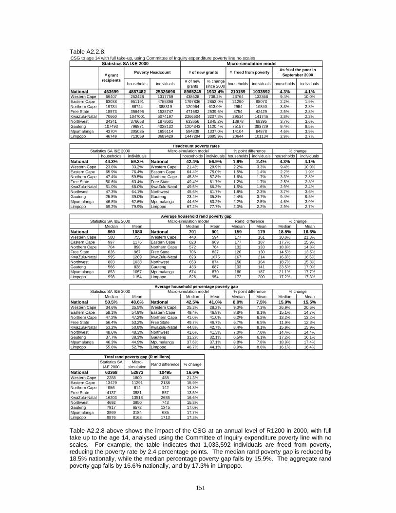
151
Table A2.2.8.
Table A2.2.8 above shows the impact of the CSG at an annual level of R1200 in 2000, with full take up to the age 14, analysed using the Committee of Inquiry expenditure poverty line with no scales. For example, the table indicates that 1,033,592 individuals are freed from poverty, reducing the poverty rate by 2.4 percentage points. The median rand poverty gap is reduced by 18.5% nationally, while the median percentage poverty gap falls by 15.9%. The aggregate rand poverty gap falls by 16.6% nationally, and by 17.3% in Limpopo.
CSG to age 14 with full take-up, using Committee of Inquiry expenditure poverty line no scales
households individuals # of new grants
% change since 2000 households individuals households individuals
National 463699 4887482 25326696 8965245 1933.4% 210159 1033592 4.3% 4.1%Western Cape 59407 252428 1317759 438528 738.2% 23764 132368 9.4% 10.0%Eastern Cape 63038 951191 4755398 1797836 2852.0% 21290 88073 2.2% 1.9%Northern Cape 19734 88744 388319 120964 613.0% 2954 10840 3.3% 2.8%Free State 18573 356495 1538747 471682 2539.6% 8754 42429 2.5% 2.8%KwaZulu-Natal 70660 1047001 6074197 2266604 3207.8% 29514 141746 2.8% 2.3%Northwest 34341 376658 1878601 633656 1845.2% 13978 68395 3.7% 3.6%Gauteng 107493 796871 4028132 1204343 1120.4% 75157 383729 9.4% 9.5%Mpumalanga 43704 305035 1656114 584338 1337.0% 14104 64878 4.6% 3.9%Limpopo 46749 713059 3689429 1447294 3095.9% 20644 101134 2.9% 2.7%
households individuals households individuals households individuals households individualsNational 44.3% 59.3% National 42.4% 56.9% 1.9% 2.4% 4.3% 4.1%Western Cape 23.6% 33.2% Western Cape 21.4% 29.9% 2.2% 3.3% 9.4% 10.0%Eastern Cape 65.9% 76.4% Eastern Cape 64.4% 75.0% 1.5% 1.4% 2.2% 1.9%Northern Cape 47.4% 59.5% Northern Cape 45.8% 57.8% 1.6% 1.7% 3.3% 2.8%Free State 50.6% 63.4% Free State 49.4% 61.7% 1.2% 1.7% 2.5% 2.8%KwaZulu-Natal 51.0% 68.0% KwaZulu-Natal 49.5% 66.3% 1.5% 1.6% 2.9% 2.4%Northwest 47.3% 64.1% Northwest 45.6% 61.7% 1.8% 2.3% 3.7% 3.6%Gauteng 25.8% 39.0% Gauteng 23.4% 35.3% 2.4% 3.7% 9.4% 9.5%Mpumalanga 46.8% 62.6% Mpumalanga 44.6% 60.2% 2.2% 2.5% 4.6% 3.9%Limpopo 69.2% 79.9% Limpopo 67.2% 77.7% 2.0% 2.2% 2.9% 2.7%
Median Mean Median Mean Median Mean Median MeanNational 860 1080 National 701 901 159 179 18.5% 16.6%Western Cape 588 755 Western Cape 440 594 177 161 30.0% 21.3%Eastern Cape 997 1176 Eastern Cape 820 989 177 187 17.7% 15.9%Northern Cape 704 898 Northern Cape 572 764 132 133 18.8% 14.8%Free State 826 967 Free State 706 837 120 130 14.5% 13.5%KwaZulu-Natal 995 1289 KwaZulu-Natal 828 1075 167 214 16.8% 16.6%Northwest 803 1038 Northwest 653 874 150 164 18.7% 15.8%Gauteng 566 828 Gauteng 433 687 133 141 23.5% 17.0%Mpumalanga 853 1057 Mpumalanga 674 870 180 187 21.1% 17.7%Limpopo 998 1154 Limpopo 826 954 172 200 17.2% 17.3%
Median Mean Median Mean Median Mean Median MeanNational 50.5% 48.6% National 42.5% 41.0% 8.0% 7.5% 15.9% 15.5%Western Cape 34.6% 35.5% Western Cape 25.3% 28.2% 9.3% 7.3% 26.9% 20.6%Eastern Cape 58.1% 54.9% Eastern Cape 49.4% 46.8% 8.8% 8.1% 15.1% 14.7%Northern Cape 47.2% 47.2% Northern Cape 41.0% 41.0% 6.2% 6.2% 13.2% 13.2%Free State 56.4% 53.2% Free State 49.7% 46.7% 6.7% 6.5% 11.9% 12.3%KwaZulu-Natal 53.2% 50.8% KwaZulu-Natal 44.8% 42.7% 8.4% 8.1% 15.9% 15.9%Northwest 48.6% 48.3% Northwest 41.6% 41.3% 7.0% 7.0% 14.4% 14.4%Gauteng 37.7% 38.3% Gauteng 31.2% 32.1% 6.5% 6.1% 17.2% 16.1%Mpumalanga 46.3% 44.9% Mpumalanga 37.6% 37.1% 8.8% 7.8% 18.9% 17.4%Limpopo 55.6% 52.7% Limpopo 46.7% 44.1% 8.9% 8.6% 16.1% 16.4%
Statistics SA I&E 2000
Micro-simulation Rand difference % change
National 63368 52873 10495 16.6%Western Cape 2288 1800 488 21.3%Eastern Cape 13429 11291 2138 15.9%Northern Cape 956 814 142 14.8%Free State 4137 3581 557 13.5%KwaZulu-Natal 16203 13518 2685 16.6%Northwest 4692 3950 743 15.8%Gauteng 7917 6572 1345 17.0%Mpumalanga 3869 3184 685 17.7%Limpopo 9876 8163 1713 17.3%
Total rand poverty gap (R millions)
Statistics SA I&E 2000 Micro-simulation model
Micro-simulation modelStatistics SA I&E 2000
Poverty Headcount# grant
recipients
% point differenceAverage household percentage poverty gap
Average household rand poverty gap% change
% changeMicro-simulation model
% change
Headcount poverty rates
# of new grants # freed from poverty As % of the poor in September 2000
Statistics SA I&E 2000 % point difference
Statistics SA I&E 2000 Micro-simulation model Rand difference

152
Table A2.2.9.
Table A2.2.9 above shows the impact of the CSG at an annual level of R1200 in 2000, with full take up to the age 16, analysed using the Committee of Inquiry expenditure poverty line with no scales. For example, the table indicates that 1,213,609 individuals are freed from poverty, reducing the poverty rate by 2.8 percentage points. The median rand poverty gap is reduced by 21.7% nationally, while the median percentage poverty gap falls by 18.5%. The aggregate rand poverty gap falls by 19.1% nationally, and by 20.1% in Limpopo.
CSG to age 16 with full take-up, using Committee of Inquiry expenditure poverty line no scales
households individuals # of new grants
% change since 2000 households individuals households individuals
National 463699 4887482 25326696 10355186 2233.2% 247015 1213609 5.1% 4.8%Western Cape 59407 252428 1317759 507844 854.9% 28688 153664 11.4% 11.7%Eastern Cape 63038 951191 4755398 2088364 3312.9% 25453 105108 2.7% 2.2%Northern Cape 19734 88744 388319 137499 696.8% 3514 14036 4.0% 3.6%Free State 18573 356495 1538747 552399 2974.2% 10374 49453 2.9% 3.2%KwaZulu-Natal 70660 1047001 6074197 2611822 3696.3% 35422 173261 3.4% 2.9%Northwest 34341 376658 1878601 734366 2138.5% 16573 81549 4.4% 4.3%Gauteng 107493 796871 4028132 1361809 1266.9% 83893 431116 10.5% 10.7%Mpumalanga 43704 305035 1656114 678983 1553.6% 16808 78637 5.5% 4.7%Limpopo 46749 713059 3689429 1682100 3598.2% 26290 126785 3.7% 3.4%
households individuals households individuals households individuals households individualsNational 44.3% 59.3% National 42.1% 56.4% 2.2% 2.8% 5.1% 4.8%Western Cape 23.6% 33.2% Western Cape 20.9% 29.3% 2.7% 3.9% 11.4% 11.7%Eastern Cape 65.9% 76.4% Eastern Cape 64.1% 74.7% 1.8% 1.7% 2.7% 2.2%Northern Cape 47.4% 59.5% Northern Cape 45.5% 57.3% 1.9% 2.2% 4.0% 3.6%Free State 50.6% 63.4% Free State 49.1% 61.4% 1.5% 2.0% 2.9% 3.2%KwaZulu-Natal 51.0% 68.0% KwaZulu-Natal 49.2% 66.0% 1.8% 2.0% 3.5% 2.9%Northwest 47.3% 64.1% Northwest 45.3% 61.3% 2.1% 2.8% 4.4% 4.3%Gauteng 25.8% 39.0% Gauteng 23.1% 34.9% 2.7% 4.2% 10.5% 10.7%Mpumalanga 46.8% 62.6% Mpumalanga 44.2% 59.7% 2.6% 3.0% 5.5% 4.7%Limpopo 69.2% 79.9% Limpopo 66.6% 77.1% 2.6% 2.7% 3.7% 3.4%
Median Mean Median Mean Median Mean Median MeanNational 860 1080 National 674 874 187 206 21.7% 19.1%Western Cape 588 755 Western Cape 429 570 204 185 34.6% 24.5%Eastern Cape 997 1176 Eastern Cape 793 959 204 217 20.4% 18.5%Northern Cape 704 898 Northern Cape 546 746 158 152 22.5% 16.9%Free State 826 967 Free State 683 815 143 152 17.3% 15.7%KwaZulu-Natal 995 1289 KwaZulu-Natal 806 1043 190 246 19.0% 19.1%Northwest 803 1038 Northwest 619 848 184 190 22.9% 18.3%Gauteng 566 828 Gauteng 424 670 143 158 25.2% 19.1%Mpumalanga 853 1057 Mpumalanga 636 840 217 217 25.4% 20.5%Limpopo 998 1154 Limpopo 789 922 209 232 21.0% 20.1%
Median Mean Median Mean Median Mean Median MeanNational 50.5% 48.6% National 41.2% 39.9% 9.3% 8.7% 18.5% 18.0%Western Cape 34.6% 35.5% Western Cape 24.8% 27.2% 9.8% 8.3% 28.4% 23.4%Eastern Cape 58.1% 54.9% Eastern Cape 47.9% 45.4% 10.2% 9.4% 17.6% 17.2%Northern Cape 47.2% 47.2% Northern Cape 40.5% 40.1% 6.7% 7.1% 14.2% 15.0%Free State 56.4% 53.2% Free State 48.4% 45.5% 8.0% 7.7% 14.2% 14.4%KwaZulu-Natal 53.2% 50.8% KwaZulu-Natal 42.9% 41.5% 10.3% 9.3% 19.4% 18.3%Northwest 48.6% 48.3% Northwest 40.3% 40.2% 8.3% 8.1% 17.1% 16.7%Gauteng 37.7% 38.3% Gauteng 30.4% 31.4% 7.3% 6.9% 19.3% 18.0%Mpumalanga 46.3% 44.9% Mpumalanga 35.6% 35.8% 10.7% 9.0% 23.0% 20.1%Limpopo 55.6% 52.7% Limpopo 45.2% 42.7% 10.5% 10.1% 18.8% 19.1%
Statistics SA I&E 2000
Micro-simulation Rand difference % change
National 63368 51275 12093 19.1%Western Cape 2288 1726 561 24.5%Eastern Cape 13429 10949 2480 18.5%Northern Cape 956 794 162 16.9%Free State 4137 3487 651 15.7%KwaZulu-Natal 16203 13112 3091 19.1%Northwest 4692 3833 859 18.3%Gauteng 7917 6405 1512 19.1%Mpumalanga 3869 3075 794 20.5%Limpopo 9876 7893 1983 20.1%
Total rand poverty gap (R millions)
Statistics SA I&E 2000 Micro-simulation model
Micro-simulation modelStatistics SA I&E 2000
Poverty Headcount# grant
recipients
% point differenceAverage household percentage poverty gap
Average household rand poverty gap% change
% changeMicro-simulation model
% change
Headcount poverty rates
# of new grants # freed from poverty As % of the poor in September 2000
Statistics SA I&E 2000 % point difference
Statistics SA I&E 2000 Micro-simulation model Rand difference

153
Table A2.2.10.
Table A2.2.10 above shows the impact of the CSG at an annual level of R1200 in 2000, with full take up to the age 18, analysed using the Committee of Inquiry expenditure poverty line with no scales. For example, the table indicates that 1,406,082 individuals are freed from poverty, reducing the poverty rate by 3.3 percentage points. The median rand poverty gap is reduced by 24.3% nationally, while the median percentage poverty gap falls by 20.7%. The aggregate rand poverty gap falls by 21.4% nationally, and by 22.5% in Limpopo.
CSG to age 18 with full take-up, using Committee of Inquiry expenditure poverty line no scales
households individuals # of new grants
% change since 2000 households individuals households individuals
National 463699 4887482 25326696 11642986 2510.9% 286573 1406082 5.9% 5.6%Western Cape 59407 252428 1317759 566614 953.8% 31007 165480 12.3% 12.6%Eastern Cape 63038 951191 4755398 2359084 3742.3% 29188 124539 3.1% 2.6%Northern Cape 19734 88744 388319 152935 775.0% 3704 14416 4.2% 3.7%Free State 18573 356495 1538747 637130 3430.4% 12322 57084 3.5% 3.7%KwaZulu-Natal 70660 1047001 6074197 2931599 4148.9% 44504 215853 4.3% 3.6%Northwest 34341 376658 1878601 817929 2381.8% 20004 97086 5.3% 5.2%Gauteng 107493 796871 4028132 1511283 1405.9% 91535 472933 11.5% 11.7%Mpumalanga 43704 305035 1656114 770392 1762.7% 18894 88286 6.2% 5.3%Limpopo 46749 713059 3689429 1896020 4055.7% 35415 170405 5.0% 4.6%
households individuals households individuals households individuals households individualsNational 44.3% 59.3% National 41.7% 56.0% 2.6% 3.3% 5.9% 5.6%Western Cape 23.6% 33.2% Western Cape 20.7% 29.0% 2.9% 4.2% 12.3% 12.6%Eastern Cape 65.9% 76.4% Eastern Cape 63.9% 74.4% 2.0% 2.0% 3.1% 2.6%Northern Cape 47.4% 59.5% Northern Cape 45.4% 57.3% 2.0% 2.2% 4.2% 3.7%Free State 50.6% 63.4% Free State 48.9% 61.1% 1.7% 2.4% 3.5% 3.7%KwaZulu-Natal 51.0% 68.0% KwaZulu-Natal 48.7% 65.5% 2.2% 2.4% 4.3% 3.6%Northwest 47.3% 64.1% Northwest 44.8% 60.8% 2.5% 3.3% 5.3% 5.2%Gauteng 25.8% 39.0% Gauteng 22.8% 34.5% 3.0% 4.6% 11.5% 11.7%Mpumalanga 46.8% 62.6% Mpumalanga 43.9% 59.3% 2.9% 3.3% 6.2% 5.3%Limpopo 69.2% 79.9% Limpopo 65.8% 76.2% 3.4% 3.7% 5.0% 4.6%
Median Mean Median Mean Median Mean Median MeanNational 860 1080 National 651 849 209 231 24.3% 21.4%Western Cape 588 755 Western Cape 403 549 222 206 37.7% 27.3%Eastern Cape 997 1176 Eastern Cape 775 931 222 245 22.2% 20.8%Northern Cape 704 898 Northern Cape 541 729 163 168 23.2% 18.7%Free State 826 967 Free State 655 792 171 175 20.7% 18.1%KwaZulu-Natal 995 1289 KwaZulu-Natal 775 1014 220 275 22.1% 21.4%Northwest 803 1038 Northwest 607 827 196 211 24.4% 20.3%Gauteng 566 828 Gauteng 417 653 150 175 26.4% 21.2%Mpumalanga 853 1057 Mpumalanga 609 812 244 246 28.6% 23.2%Limpopo 998 1154 Limpopo 759 894 239 260 24.0% 22.5%
Median Mean Median Mean Median Mean Median MeanNational 50.5% 48.6% National 40.1% 38.7% 10.4% 9.8% 20.7% 20.3%Western Cape 34.6% 35.5% Western Cape 23.6% 26.3% 10.9% 9.2% 31.7% 25.9%Eastern Cape 58.1% 54.9% Eastern Cape 46.6% 44.1% 11.5% 10.8% 19.8% 19.6%Northern Cape 47.2% 47.2% Northern Cape 39.5% 39.3% 7.7% 7.9% 16.4% 16.7%Free State 56.4% 53.2% Free State 47.2% 44.2% 9.2% 9.0% 16.3% 16.9%KwaZulu-Natal 53.2% 50.8% KwaZulu-Natal 42.1% 40.3% 11.1% 10.5% 20.8% 20.6%Northwest 48.6% 48.3% Northwest 39.6% 39.3% 9.0% 9.0% 18.5% 18.6%Gauteng 37.7% 38.3% Gauteng 29.4% 30.7% 8.3% 7.6% 21.9% 19.9%Mpumalanga 46.3% 44.9% Mpumalanga 34.9% 34.7% 11.4% 10.2% 24.6% 22.8%Limpopo 55.6% 52.7% Limpopo 43.1% 41.4% 12.5% 11.4% 22.6% 21.6%
Statistics SA I&E 2000
Micro-simulation Rand difference % change
National 63368 49800 13569 21.4%Western Cape 2288 1663 625 27.3%Eastern Cape 13429 10630 2799 20.8%Northern Cape 956 777 179 18.7%Free State 4137 3388 749 18.1%KwaZulu-Natal 16203 12743 3460 21.4%Northwest 4692 3738 955 20.3%Gauteng 7917 6240 1677 21.2%Mpumalanga 3869 2971 899 23.2%Limpopo 9876 7650 2226 22.5%
Total rand poverty gap (R millions)
Statistics SA I&E 2000 Micro-simulation model
Micro-simulation modelStatistics SA I&E 2000
Poverty Headcount# grant
recipients
% point differenceAverage household percentage poverty gap
Average household rand poverty gap% change
% changeMicro-simulation model
% change
Headcount poverty rates
# of new grants # freed from poverty As % of the poor in September 2000
Statistics SA I&E 2000 % point difference
Statistics SA I&E 2000 Micro-simulation model Rand difference

154
Table A2.2.11.
Table A2.2.11 above shows the impact of the CSG at an annual level of R1606 in 2000, with full take up to the age 7, analysed using the Committee of Inquiry expenditure poverty line with no scales. For example, the table indicates that 585,019 individuals are freed from poverty, reducing the poverty rate by 1.4 percentage points. The median rand poverty gap is reduced by 11.3% nationally, while the median percentage poverty gap falls by 8.9%. The aggregate rand poverty gap falls by 10.0% nationally, and by 10.3% in Limpopo.
CSG(1606) to age 7 with full take-up, using Committee of Inquiry expenditure poverty line with no scales
households individuals # of new grants
% change since 2000 households individuals households individuals
National 463699 4887482 25326696 4026590 868.4% 125457 585019 2.6% 2.3%Western Cape 59407 252428 1317759 210409 354.2% 17115 90240 6.8% 6.8%Eastern Cape 63038 951191 4755398 769172 1220.2% 8043 36915 0.8% 0.8%Northern Cape 19734 88744 388319 60684 307.5% 2102 6973 2.4% 1.8%Free State 18573 356495 1538747 202617 1090.9% 5066 22313 1.4% 1.5%KwaZulu-Natal 70660 1047001 6074197 1042611 1475.5% 17902 74849 1.7% 1.2%Northwest 34341 376658 1878601 274279 798.7% 9168 41466 2.4% 2.2%Gauteng 107493 796871 4028132 574022 534.0% 49576 235214 6.2% 5.8%Mpumalanga 43704 305035 1656114 250306 572.7% 7728 31149 2.5% 1.9%Limpopo 46749 713059 3689429 642490 1374.3% 8757 45900 1.2% 1.2%
households individuals households individuals households individuals households individualsNational 44.3% 59.3% National 43.2% 57.9% 1.1% 1.4% 2.6% 2.3%Western Cape 23.6% 33.2% Western Cape 22.0% 30.9% 1.6% 2.3% 6.8% 6.8%Eastern Cape 65.9% 76.4% Eastern Cape 65.3% 75.8% 0.6% 0.6% 0.8% 0.8%Northern Cape 47.4% 59.5% Northern Cape 46.3% 58.4% 1.1% 1.1% 2.4% 1.8%Free State 50.6% 63.4% Free State 49.9% 62.5% 0.7% 0.9% 1.4% 1.5%KwaZulu-Natal 51.0% 68.0% KwaZulu-Natal 50.1% 67.1% 0.9% 0.8% 1.7% 1.2%Northwest 47.3% 64.1% Northwest 46.2% 62.7% 1.2% 1.4% 2.4% 2.2%Gauteng 25.8% 39.0% Gauteng 24.2% 36.8% 1.6% 2.3% 6.2% 5.8%Mpumalanga 46.8% 62.6% Mpumalanga 45.6% 61.5% 1.2% 1.2% 2.5% 1.9%Limpopo 69.2% 79.9% Limpopo 68.3% 78.9% 0.8% 1.0% 1.2% 1.2%
Median Mean Median Mean Median Mean Median MeanNational 860 1080 National 764 973 97 108 11.3% 10.0%Western Cape 588 755 Western Cape 494 651 97 104 16.4% 13.8%Eastern Cape 997 1176 Eastern Cape 900 1069 97 107 9.7% 9.1%Northern Cape 704 898 Northern Cape 618 808 86 89 12.2% 9.9%Free State 826 967 Free State 747 892 79 75 9.6% 7.8%KwaZulu-Natal 995 1289 KwaZulu-Natal 899 1157 96 132 9.7% 10.2%Northwest 803 1038 Northwest 718 943 85 95 10.5% 9.2%Gauteng 566 828 Gauteng 494 738 72 90 12.8% 10.9%Mpumalanga 853 1057 Mpumalanga 737 950 116 107 13.6% 10.2%Limpopo 998 1154 Limpopo 910 1035 88 119 8.8% 10.3%
Median Mean Median Mean Median Mean Median MeanNational 50.5% 48.6% National 46.0% 44.0% 4.5% 4.5% 8.9% 9.3%Western Cape 34.6% 35.5% Western Cape 29.1% 30.7% 5.5% 4.8% 15.9% 13.6%Eastern Cape 58.1% 54.9% Eastern Cape 53.0% 50.3% 5.1% 4.6% 8.8% 8.3%Northern Cape 47.2% 47.2% Northern Cape 43.3% 42.9% 3.9% 4.3% 8.2% 9.0%Free State 56.4% 53.2% Free State 51.7% 49.4% 4.7% 3.8% 8.3% 7.1%KwaZulu-Natal 53.2% 50.8% KwaZulu-Natal 47.9% 45.8% 5.2% 4.9% 9.9% 9.7%Northwest 48.6% 48.3% Northwest 43.7% 44.3% 4.9% 4.0% 10.1% 8.2%Gauteng 37.7% 38.3% Gauteng 32.8% 34.2% 4.9% 4.1% 12.9% 10.7%Mpumalanga 46.3% 44.9% Mpumalanga 41.3% 40.4% 5.0% 4.5% 10.8% 9.9%Limpopo 55.6% 52.7% Limpopo 50.4% 47.7% 5.3% 5.0% 9.5% 9.5%
Statistics SA I&E 2000
Micro-simulation Rand difference % change
National 63368 57047 6321 10.0%Western Cape 2288 1973 315 13.8%Eastern Cape 13429 12204 1225 9.1%Northern Cape 956 861 95 9.9%Free State 4137 3817 321 7.8%KwaZulu-Natal 16203 14545 1658 10.2%Northwest 4692 4261 431 9.2%Gauteng 7917 7056 861 10.9%Mpumalanga 3869 3477 393 10.2%Limpopo 9876 8855 1021 10.3%
% change
Headcount poverty rates
# of new grants # freed from poverty As % of the poor in September 2000
Statistics SA I&E 2000 % point difference
Statistics SA I&E 2000 Micro-simulation model Rand differenceAverage household rand poverty gap
% change
% changeMicro-simulation model
Total rand poverty gap (R millions)
Statistics SA I&E 2000 Micro-simulation model
Micro-simulation modelStatistics SA I&E 2000
Poverty Headcount# grant
recipients
% point differenceAverage household percentage poverty gap

155
Table A2.2.12.
Table A2.2.12 above shows the impact of the CSG at an annual level of R1606 in 2000, with full take up to the age 9, analysed using the Committee of Inquiry expenditure poverty line with no scales. For example, the table indicates that 840,046 individuals are freed from poverty, reducing the poverty rate by 2.0 percentage points. The median rand poverty gap is reduced by 14.8% nationally, while the median percentage poverty gap falls by 12.3%. The aggregate rand poverty gap falls by 13.4% nationally, and by 13.8% in Limpopo.
CSG(1606) to age 9 with full take-up, using Committee of Inquiry expenditure poverty line with no scales
households individuals # of new grants
% change since 2000 households individuals households individuals
National 463699 4887482 25326696 5413470 1167.5% 173417 840046 3.5% 3.3%Western Cape 59407 252428 1317759 274483 462.0% 19507 104631 7.7% 7.9%Eastern Cape 63038 951191 4755398 1045120 1657.9% 14449 66545 1.5% 1.4%Northern Cape 19734 88744 388319 77530 392.9% 3247 11121 3.7% 2.9%Free State 18573 356495 1538747 278621 1500.1% 6932 32679 1.9% 2.1%KwaZulu-Natal 70660 1047001 6074197 1403055 1985.6% 25208 110751 2.4% 1.8%Northwest 34341 376658 1878601 372722 1085.4% 13562 62878 3.6% 3.3%Gauteng 107493 796871 4028132 755032 702.4% 63484 320779 8.0% 8.0%Mpumalanga 43704 305035 1656114 346442 792.7% 10567 44489 3.5% 2.7%Limpopo 46749 713059 3689429 860465 1840.6% 16461 86173 2.3% 2.3%
households individuals households individuals households individuals households individualsNational 44.3% 59.3% National 42.8% 57.3% 1.6% 2.0% 3.5% 3.3%Western Cape 23.6% 33.2% Western Cape 21.8% 30.6% 1.8% 2.6% 7.7% 7.9%Eastern Cape 65.9% 76.4% Eastern Cape 64.9% 75.3% 1.0% 1.1% 1.5% 1.4%Northern Cape 47.4% 59.5% Northern Cape 45.7% 57.8% 1.7% 1.7% 3.7% 2.9%Free State 50.6% 63.4% Free State 49.6% 62.1% 1.0% 1.3% 1.9% 2.1%KwaZulu-Natal 51.0% 68.0% KwaZulu-Natal 49.7% 66.7% 1.2% 1.2% 2.4% 1.8%Northwest 47.3% 64.1% Northwest 45.6% 61.9% 1.7% 2.1% 3.6% 3.3%Gauteng 25.8% 39.0% Gauteng 23.7% 35.9% 2.1% 3.1% 8.0% 8.0%Mpumalanga 46.8% 62.6% Mpumalanga 45.2% 60.9% 1.6% 1.7% 3.5% 2.7%Limpopo 69.2% 79.9% Limpopo 67.6% 78.0% 1.6% 1.9% 2.3% 2.3%
Median Mean Median Mean Median Mean Median MeanNational 860 1080 National 733 936 127 144 14.8% 13.4%Western Cape 588 755 Western Cape 453 620 132 135 22.4% 17.9%Eastern Cape 997 1176 Eastern Cape 865 1031 132 146 13.2% 12.4%Northern Cape 704 898 Northern Cape 585 784 120 113 17.0% 12.6%Free State 826 967 Free State 732 864 94 103 11.4% 10.6%KwaZulu-Natal 995 1289 KwaZulu-Natal 862 1112 133 177 13.4% 13.8%Northwest 803 1038 Northwest 678 909 125 129 15.6% 12.4%Gauteng 566 828 Gauteng 460 710 107 118 18.8% 14.2%Mpumalanga 853 1057 Mpumalanga 701 909 153 148 17.9% 14.0%Limpopo 998 1154 Limpopo 855 995 143 159 14.4% 13.8%
Median Mean Median Mean Median Mean Median MeanNational 50.5% 48.6% National 44.3% 42.5% 6.2% 6.1% 12.3% 12.5%Western Cape 34.6% 35.5% Western Cape 27.5% 29.3% 7.1% 6.2% 20.5% 17.4%Eastern Cape 58.1% 54.9% Eastern Cape 51.2% 48.7% 6.9% 6.2% 11.9% 11.3%Northern Cape 47.2% 47.2% Northern Cape 41.6% 41.8% 5.5% 5.4% 11.7% 11.4%Free State 56.4% 53.2% Free State 50.3% 48.0% 6.1% 5.2% 10.8% 9.8%KwaZulu-Natal 53.2% 50.8% KwaZulu-Natal 46.3% 44.1% 6.9% 6.7% 12.9% 13.1%Northwest 48.6% 48.3% Northwest 42.7% 42.9% 5.9% 5.4% 12.1% 11.2%Gauteng 37.7% 38.3% Gauteng 31.9% 33.0% 5.8% 5.3% 15.5% 13.9%Mpumalanga 46.3% 44.9% Mpumalanga 39.3% 38.7% 7.0% 6.2% 15.1% 13.7%Limpopo 55.6% 52.7% Limpopo 48.9% 46.0% 6.7% 6.8% 12.0% 12.8%
Statistics SA I&E 2000
Micro-simulation Rand difference % change
National 63368 54895 8474 13.4%Western Cape 2288 1879 409 17.9%Eastern Cape 13429 11767 1662 12.4%Northern Cape 956 835 121 12.6%Free State 4137 3697 440 10.6%KwaZulu-Natal 16203 13974 2229 13.8%Northwest 4692 4110 582 12.4%Gauteng 7917 6789 1128 14.2%Mpumalanga 3869 3327 542 14.0%Limpopo 9876 8517 1359 13.8%
% change
Headcount poverty rates
# of new grants # freed from poverty As % of the poor in September 2000
Statistics SA I&E 2000 % point difference
Statistics SA I&E 2000 Micro-simulation model Rand differenceAverage household rand poverty gap
% change
% changeMicro-simulation model
Total rand poverty gap (R millions)
Statistics SA I&E 2000 Micro-simulation model
Micro-simulation modelStatistics SA I&E 2000
Poverty Headcount# grant
recipients
% point differenceAverage household percentage poverty gap

156
Table A2.2.13.
Table A2.2.13 above shows the impact of the CSG at an annual level of R1606 in 2000, with full take up to the age 11, analysed using the Committee of Inquiry expenditure poverty line with no scales. For example, the table indicates that 1,072,843 individuals are freed from poverty, reducing the poverty rate by 2.5 percentage points. The median rand poverty gap is reduced by 18.9% nationally, while the median percentage poverty gap falls by 16.3%. The aggregate rand poverty gap falls by 16.9% nationally, and by 17.5% in Limpopo.
CSG(1606) to age 11 with full take-up, using Committee of Inquiry expenditure poverty line with no scales
households individuals # of new grants
% change since 2000 households individuals households individuals
National 463699 4887482 25326696 6868586 1481.3% 220717 1072843 4.5% 4.2%Western Cape 59407 252428 1317759 351636 591.9% 24228 133503 9.6% 10.1%Eastern Cape 63038 951191 4755398 1350604 2142.5% 22725 106529 2.4% 2.2%Northern Cape 19734 88744 388319 95993 486.4% 3543 12499 4.0% 3.2%Free State 18573 356495 1538747 357842 1926.7% 7690 36217 2.2% 2.4%KwaZulu-Natal 70660 1047001 6074197 1753054 2481.0% 36494 162962 3.5% 2.7%Northwest 34341 376658 1878601 480447 1399.0% 16257 76676 4.3% 4.1%Gauteng 107493 796871 4028132 938656 873.2% 74365 376816 9.3% 9.4%Mpumalanga 43704 305035 1656114 440428 1007.8% 14296 64141 4.7% 3.9%Limpopo 46749 713059 3689429 1099926 2352.8% 21119 103500 3.0% 2.8%
households individuals households individuals households individuals households individualsNational 44.3% 59.3% National 42.3% 56.8% 2.0% 2.5% 4.5% 4.2%Western Cape 23.6% 33.2% Western Cape 21.3% 29.8% 2.3% 3.4% 9.6% 10.1%Eastern Cape 65.9% 76.4% Eastern Cape 64.3% 74.7% 1.6% 1.7% 2.4% 2.2%Northern Cape 47.4% 59.5% Northern Cape 45.5% 57.6% 1.9% 1.9% 4.0% 3.2%Free State 50.6% 63.4% Free State 49.5% 61.9% 1.1% 1.5% 2.2% 2.4%KwaZulu-Natal 51.0% 68.0% KwaZulu-Natal 49.2% 66.1% 1.8% 1.8% 3.5% 2.7%Northwest 47.3% 64.1% Northwest 45.3% 61.5% 2.0% 2.6% 4.3% 4.1%Gauteng 25.8% 39.0% Gauteng 23.4% 35.4% 2.4% 3.7% 9.3% 9.4%Mpumalanga 46.8% 62.6% Mpumalanga 44.6% 60.2% 2.2% 2.4% 4.7% 3.9%Limpopo 69.2% 79.9% Limpopo 67.1% 77.6% 2.0% 2.2% 3.0% 2.8%
Median Mean Median Mean Median Mean Median MeanNational 860 1080 National 698 898 162 182 18.9% 16.9%Western Cape 588 755 Western Cape 431 585 178 170 30.3% 22.5%Eastern Cape 997 1176 Eastern Cape 819 989 178 188 17.9% 16.0%Northern Cape 704 898 Northern Cape 568 757 136 140 19.3% 15.6%Free State 826 967 Free State 710 835 116 132 14.0% 13.7%KwaZulu-Natal 995 1289 KwaZulu-Natal 827 1068 168 221 16.9% 17.1%Northwest 803 1038 Northwest 659 872 144 166 17.9% 16.0%Gauteng 566 828 Gauteng 423 683 143 145 25.3% 17.5%Mpumalanga 853 1057 Mpumalanga 673 869 181 188 21.2% 17.8%Limpopo 998 1154 Limpopo 814 952 184 203 18.4% 17.5%
Median Mean Median Mean Median Mean Median MeanNational 50.5% 48.6% National 42.3% 40.9% 8.2% 7.7% 16.3% 15.8%Western Cape 34.6% 35.5% Western Cape 26.0% 27.8% 8.6% 7.7% 24.8% 21.8%Eastern Cape 58.1% 54.9% Eastern Cape 49.2% 46.9% 9.0% 8.0% 15.4% 14.6%Northern Cape 47.2% 47.2% Northern Cape 40.4% 40.6% 6.8% 6.6% 14.5% 13.9%Free State 56.4% 53.2% Free State 49.1% 46.6% 7.4% 6.6% 13.0% 12.5%KwaZulu-Natal 53.2% 50.8% KwaZulu-Natal 44.5% 42.5% 8.7% 8.3% 16.4% 16.3%Northwest 48.6% 48.3% Northwest 41.2% 41.3% 7.4% 7.0% 15.3% 14.5%Gauteng 37.7% 38.3% Gauteng 30.5% 31.9% 7.3% 6.4% 19.2% 16.8%Mpumalanga 46.3% 44.9% Mpumalanga 37.6% 37.1% 8.7% 7.8% 18.7% 17.4%Limpopo 55.6% 52.7% Limpopo 47.1% 44.1% 8.5% 8.7% 15.4% 16.4%
Statistics SA I&E 2000
Micro-simulation Rand difference % change
National 63368 52665 10704 16.9%Western Cape 2288 1773 514 22.5%Eastern Cape 13429 11286 2143 16.0%Northern Cape 956 807 149 15.6%Free State 4137 3572 566 13.7%KwaZulu-Natal 16203 13429 2774 17.1%Northwest 4692 3943 749 16.0%Gauteng 7917 6530 1387 17.5%Mpumalanga 3869 3181 688 17.8%Limpopo 9876 8143 1733 17.5%
% change
Headcount poverty rates
# of new grants # freed from poverty As % of the poor in September 2000
Statistics SA I&E 2000 % point difference
Statistics SA I&E 2000 Micro-simulation model Rand differenceAverage household rand poverty gap
% change
% changeMicro-simulation model
Total rand poverty gap (R millions)
Statistics SA I&E 2000 Micro-simulation model
Micro-simulation modelStatistics SA I&E 2000
Poverty Headcount# grant
recipients
% point differenceAverage household percentage poverty gap

157
Table A2.2.14.
Table A2.2.14 above shows the impact of the CSG at an annual level of R1606 in 2000, with full take up to the age 14, analysed using the Committee of Inquiry expenditure poverty line with no scales. For example, the table indicates that 1,420,330 individuals are freed from poverty, reducing the poverty rate by 3.3 percentage points. The median rand poverty gap is reduced by 24.6% nationally, while the median percentage poverty gap falls by 21.2%. The aggregate rand poverty gap falls by 22.0% nationally, and by 23.1% in Limpopo.
CSG(1606) to age 14 with full take-up, using Committee of Inquiry expenditure poverty line with no scales
households individuals # of new grants
% change since 2000 households individuals households individuals
National 463699 4887482 25326696 8965245 1933.4% 288869 1420330 5.9% 5.6%Western Cape 59407 252428 1317759 438528 738.2% 30113 165778 11.9% 12.6%Eastern Cape 63038 951191 4755398 1797836 2852.0% 29835 134826 3.1% 2.8%Northern Cape 19734 88744 388319 120964 613.0% 3937 14595 4.4% 3.8%Free State 18573 356495 1538747 471682 2539.6% 11145 51276 3.1% 3.3%KwaZulu-Natal 70660 1047001 6074197 2266604 3207.8% 48761 232187 4.7% 3.8%Northwest 34341 376658 1878601 633656 1845.2% 20934 101202 5.6% 5.4%Gauteng 107493 796871 4028132 1204343 1120.4% 93971 475414 11.8% 11.8%Mpumalanga 43704 305035 1656114 584338 1337.0% 21871 102141 7.2% 6.2%Limpopo 46749 713059 3689429 1447294 3095.9% 28302 142911 4.0% 3.9%
households individuals households individuals households individuals households individualsNational 44.3% 59.3% National 41.7% 56.0% 2.6% 3.3% 5.9% 5.6%Western Cape 23.6% 33.2% Western Cape 20.8% 29.0% 2.8% 4.2% 11.9% 12.6%Eastern Cape 65.9% 76.4% Eastern Cape 63.8% 74.2% 2.1% 2.2% 3.1% 2.8%Northern Cape 47.4% 59.5% Northern Cape 45.3% 57.2% 2.1% 2.2% 4.4% 3.8%Free State 50.6% 63.4% Free State 49.0% 61.3% 1.6% 2.1% 3.1% 3.3%KwaZulu-Natal 51.0% 68.0% KwaZulu-Natal 48.6% 65.4% 2.4% 2.6% 4.7% 3.8%Northwest 47.3% 64.1% Northwest 44.7% 60.6% 2.6% 3.5% 5.6% 5.4%Gauteng 25.8% 39.0% Gauteng 22.7% 34.4% 3.0% 4.6% 11.8% 11.8%Mpumalanga 46.8% 62.6% Mpumalanga 43.4% 58.8% 3.4% 3.9% 7.2% 6.2%Limpopo 69.2% 79.9% Limpopo 66.4% 76.8% 2.7% 3.1% 4.0% 3.9%
Median Mean Median Mean Median Mean Median MeanNational 860 1080 National 649 843 212 237 24.6% 22.0%Western Cape 588 755 Western Cape 388 544 236 212 40.1% 28.0%Eastern Cape 997 1176 Eastern Cape 761 927 236 250 23.6% 21.2%Northern Cape 704 898 Northern Cape 533 720 172 177 24.4% 19.7%Free State 826 967 Free State 664 794 162 173 19.6% 17.9%KwaZulu-Natal 995 1289 KwaZulu-Natal 775 1005 221 284 22.2% 22.0%Northwest 803 1038 Northwest 607 820 196 218 24.4% 21.0%Gauteng 566 828 Gauteng 384 644 183 184 32.2% 22.2%Mpumalanga 853 1057 Mpumalanga 603 809 250 248 29.3% 23.5%Limpopo 998 1154 Limpopo 758 888 240 266 24.1% 23.1%
Median Mean Median Mean Median Mean Median MeanNational 50.5% 48.6% National 39.8% 38.6% 10.7% 10.0% 21.2% 20.6%Western Cape 34.6% 35.5% Western Cape 22.6% 25.9% 12.0% 9.6% 34.6% 27.0%Eastern Cape 58.1% 54.9% Eastern Cape 46.4% 44.1% 11.8% 10.7% 20.3% 19.6%Northern Cape 47.2% 47.2% Northern Cape 39.2% 38.9% 8.0% 8.2% 16.9% 17.5%Free State 56.4% 53.2% Free State 47.3% 44.5% 9.1% 8.7% 16.2% 16.3%KwaZulu-Natal 53.2% 50.8% KwaZulu-Natal 41.9% 40.1% 11.3% 10.7% 21.3% 21.1%Northwest 48.6% 48.3% Northwest 39.4% 39.1% 9.2% 9.2% 18.9% 19.1%Gauteng 37.7% 38.3% Gauteng 29.1% 30.3% 8.6% 8.0% 22.9% 20.9%Mpumalanga 46.3% 44.9% Mpumalanga 34.7% 34.6% 11.6% 10.3% 25.0% 22.9%Limpopo 55.6% 52.7% Limpopo 43.1% 41.3% 12.5% 11.5% 22.5% 21.8%
Statistics SA I&E 2000
Micro-simulation Rand difference % change
National 63368 49447 13921 22.0%Western Cape 2288 1647 641 28.0%Eastern Cape 13429 10580 2849 21.2%Northern Cape 956 767 189 19.7%Free State 4137 3397 740 17.9%KwaZulu-Natal 16203 12631 3572 22.0%Northwest 4692 3708 985 21.0%Gauteng 7917 6157 1760 22.2%Mpumalanga 3869 2962 907 23.5%Limpopo 9876 7598 2278 23.1%
% change
Headcount poverty rates
# of new grants # freed from poverty As % of the poor in September 2000
Statistics SA I&E 2000 % point difference
Statistics SA I&E 2000 Micro-simulation model Rand differenceAverage household rand poverty gap
% change
% changeMicro-simulation model
Total rand poverty gap (R millions)
Statistics SA I&E 2000 Micro-simulation model
Micro-simulation modelStatistics SA I&E 2000
Poverty Headcount# grant
recipients
% point differenceAverage household percentage poverty gap

158
Table A2.2.15.
Table A2.2.15 above shows the impact of the CSG at an annual level of R1606 in 2000, with full take up to the age 16, analysed using the Committee of Inquiry expenditure poverty line with no scales. For example, the table indicates that 1,637,527 individuals are freed from poverty, reducing the poverty rate by 3.8 percentage points. The median rand poverty gap is reduced by 28.4% nationally, while the median percentage poverty gap falls by 24.6%. The aggregate rand poverty gap falls by 25.3% nationally, and by 26.7% in Limpopo.
CSG(1606) to age 16 with full take-up, using Committee of Inquiry expenditure poverty line with no scales
households individuals # of new grants
% change since 2000 households individuals households individuals
National 463699 4887482 25326696 10355186 2233.2% 336009 1637527 6.9% 6.5%Western Cape 59407 252428 1317759 507844 854.9% 36079 189512 14.3% 14.4%Eastern Cape 63038 951191 4755398 2088364 3312.9% 34886 153796 3.7% 3.2%Northern Cape 19734 88744 388319 137499 696.8% 4451 18379 5.0% 4.7%Free State 18573 356495 1538747 552399 2974.2% 13400 61610 3.8% 4.0%KwaZulu-Natal 70660 1047001 6074197 2611822 3696.3% 53665 253190 5.1% 4.2%Northwest 34341 376658 1878601 734366 2138.5% 24312 120684 6.5% 6.4%Gauteng 107493 796871 4028132 1361809 1266.9% 105139 533656 13.2% 13.2%Mpumalanga 43704 305035 1656114 678983 1553.6% 25677 122442 8.4% 7.4%Limpopo 46749 713059 3689429 1682100 3598.2% 38400 184258 5.4% 5.0%
households individuals households individuals households individuals households individualsNational 44.3% 59.3% National 41.3% 55.5% 3.0% 3.8% 6.9% 6.5%Western Cape 23.6% 33.2% Western Cape 20.2% 28.4% 3.4% 4.8% 14.3% 14.4%Eastern Cape 65.9% 76.4% Eastern Cape 63.5% 73.9% 2.4% 2.5% 3.7% 3.2%Northern Cape 47.4% 59.5% Northern Cape 45.0% 56.7% 2.4% 2.8% 5.0% 4.7%Free State 50.6% 63.4% Free State 48.7% 60.9% 1.9% 2.5% 3.8% 4.0%KwaZulu-Natal 51.0% 68.0% KwaZulu-Natal 48.3% 65.1% 2.6% 2.8% 5.1% 4.2%Northwest 47.3% 64.1% Northwest 44.3% 60.0% 3.1% 4.1% 6.5% 6.4%Gauteng 25.8% 39.0% Gauteng 22.4% 33.9% 3.4% 5.2% 13.2% 13.2%Mpumalanga 46.8% 62.6% Mpumalanga 42.8% 58.0% 3.9% 4.6% 8.4% 7.4%Limpopo 69.2% 79.9% Limpopo 65.5% 75.9% 3.7% 4.0% 5.4% 5.0%
Median Mean Median Mean Median Mean Median MeanNational 860 1080 National 616 807 245 273 28.4% 25.3%Western Cape 588 755 Western Cape 367 512 272 243 46.3% 32.2%Eastern Cape 997 1176 Eastern Cape 724 887 272 289 27.3% 24.6%Northern Cape 704 898 Northern Cape 499 697 205 201 29.1% 22.4%Free State 826 967 Free State 637 765 189 202 22.8% 20.9%KwaZulu-Natal 995 1289 KwaZulu-Natal 722 962 273 327 27.4% 25.4%Northwest 803 1038 Northwest 574 786 229 252 28.5% 24.3%Gauteng 566 828 Gauteng 377 621 189 207 33.4% 25.0%Mpumalanga 853 1057 Mpumalanga 563 770 290 287 34.0% 27.2%Limpopo 998 1154 Limpopo 710 846 288 308 28.9% 26.7%
Median Mean Median Mean Median Mean Median MeanNational 50.5% 48.6% National 38.1% 37.0% 12.5% 11.5% 24.6% 23.8%Western Cape 34.6% 35.5% Western Cape 21.0% 24.6% 13.6% 10.9% 39.3% 30.6%Eastern Cape 58.1% 54.9% Eastern Cape 44.2% 42.3% 14.0% 12.6% 24.0% 22.9%Northern Cape 47.2% 47.2% Northern Cape 38.2% 37.8% 9.0% 9.4% 19.0% 19.8%Free State 56.4% 53.2% Free State 45.8% 43.0% 10.6% 10.2% 18.8% 19.2%KwaZulu-Natal 53.2% 50.8% KwaZulu-Natal 40.3% 38.4% 12.9% 12.4% 24.2% 24.3%Northwest 48.6% 48.3% Northwest 38.0% 37.6% 10.6% 10.6% 21.8% 22.0%Gauteng 37.7% 38.3% Gauteng 28.1% 29.3% 9.6% 9.0% 25.4% 23.5%Mpumalanga 46.3% 44.9% Mpumalanga 32.9% 33.0% 13.5% 11.9% 29.1% 26.5%Limpopo 55.6% 52.7% Limpopo 41.1% 39.4% 14.5% 13.4% 26.1% 25.3%
Statistics SA I&E 2000
Micro-simulation Rand difference % change
National 63368 47338 16030 25.3%Western Cape 2288 1551 736 32.2%Eastern Cape 13429 10125 3304 24.6%Northern Cape 956 742 214 22.4%Free State 4137 3273 865 20.9%KwaZulu-Natal 16203 12092 4111 25.4%Northwest 4692 3554 1138 24.3%Gauteng 7917 5940 1978 25.0%Mpumalanga 3869 2819 1051 27.2%Limpopo 9876 7242 2634 26.7%
% change
Headcount poverty rates
# of new grants # freed from poverty As % of the poor in September 2000
Statistics SA I&E 2000 % point difference
Statistics SA I&E 2000 Micro-simulation model Rand differenceAverage household rand poverty gap
% change
% changeMicro-simulation model
Total rand poverty gap (R millions)
Statistics SA I&E 2000 Micro-simulation model
Micro-simulation modelStatistics SA I&E 2000
Poverty Headcount# grant
recipients
% point differenceAverage household percentage poverty gap
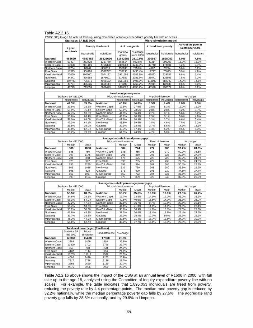
159
Table A2.2.16.
Table A2.2.16 above shows the impact of the CSG at an annual level of R1606 in 2000, with full take up to the age 18, analysed using the Committee of Inquiry expenditure poverty line with no scales. For example, the table indicates that 1,895,053 individuals are freed from poverty, reducing the poverty rate by 4.4 percentage points. The median rand poverty gap is reduced by 32.2% nationally, while the median percentage poverty gap falls by 27.5%. The aggregate rand poverty gap falls by 28.3% nationally, and by 29.9% in Limpopo.
CSG(1606) to age 18 with full take-up, using Committee of Inquiry expenditure poverty line with no scales
households individuals # of new grants
% change since 2000 households individuals households individuals
National 463699 4887482 25326696 11642986 2510.9% 390957 1895053 8.0% 7.5%Western Cape 59407 252428 1317759 566614 953.8% 40314 209293 16.0% 15.9%Eastern Cape 63038 951191 4755398 2359084 3742.3% 39740 174501 4.2% 3.7%Northern Cape 19734 88744 388319 152935 775.0% 4982 20274 5.6% 5.2%Free State 18573 356495 1538747 637130 3430.4% 17727 75073 5.0% 4.9%KwaZulu-Natal 70660 1047001 6074197 2931599 4148.9% 68833 329757 6.6% 5.4%Northwest 34341 376658 1878601 817929 2381.8% 28071 135696 7.5% 7.2%Gauteng 107493 796871 4028132 1511283 1405.9% 113809 582249 14.3% 14.5%Mpumalanga 43704 305035 1656114 770392 1762.7% 28911 137633 9.5% 8.3%Limpopo 46749 713059 3689429 1896020 4055.7% 48570 230577 6.8% 6.2%
households individuals households individuals households individuals households individualsNational 44.3% 59.3% National 40.8% 54.8% 3.5% 4.4% 8.0% 7.5%Western Cape 23.6% 33.2% Western Cape 19.8% 27.9% 3.8% 5.3% 16.0% 15.9%Eastern Cape 65.9% 76.4% Eastern Cape 63.1% 73.6% 2.8% 2.8% 4.2% 3.7%Northern Cape 47.4% 59.5% Northern Cape 44.8% 56.4% 2.7% 3.1% 5.6% 5.2%Free State 50.6% 63.4% Free State 48.1% 60.3% 2.5% 3.1% 5.0% 4.9%KwaZulu-Natal 51.0% 68.0% KwaZulu-Natal 47.6% 64.3% 3.3% 3.7% 6.6% 5.4%Northwest 47.3% 64.1% Northwest 43.8% 59.5% 3.5% 4.6% 7.5% 7.2%Gauteng 25.8% 39.0% Gauteng 22.1% 33.4% 3.7% 5.6% 14.3% 14.5%Mpumalanga 46.8% 62.6% Mpumalanga 42.3% 57.4% 4.4% 5.2% 9.5% 8.3%Limpopo 69.2% 79.9% Limpopo 64.5% 74.9% 4.7% 5.0% 6.8% 6.2%
Median Mean Median Mean Median Mean Median MeanNational 860 1080 National 584 774 277 306 32.2% 28.3%Western Cape 588 755 Western Cape 335 485 295 270 50.2% 35.8%Eastern Cape 997 1176 Eastern Cape 701 850 295 326 29.6% 27.7%Northern Cape 704 898 Northern Cape 477 675 227 223 32.2% 24.9%Free State 826 967 Free State 599 735 227 232 27.5% 24.0%KwaZulu-Natal 995 1289 KwaZulu-Natal 691 924 304 365 30.6% 28.3%Northwest 803 1038 Northwest 539 759 263 280 32.8% 26.9%Gauteng 566 828 Gauteng 371 599 195 229 34.5% 27.7%Mpumalanga 853 1057 Mpumalanga 550 732 304 325 35.6% 30.7%Limpopo 998 1154 Limpopo 673 809 325 345 32.5% 29.9%
Median Mean Median Mean Median Mean Median MeanNational 50.5% 48.6% National 36.7% 35.6% 13.9% 13.0% 27.5% 26.7%Western Cape 34.6% 35.5% Western Cape 19.7% 23.5% 14.9% 12.0% 43.0% 33.9%Eastern Cape 58.1% 54.9% Eastern Cape 42.6% 40.6% 15.6% 14.3% 26.8% 26.0%Northern Cape 47.2% 47.2% Northern Cape 37.5% 36.7% 9.7% 10.5% 20.6% 22.1%Free State 56.4% 53.2% Free State 44.6% 41.3% 11.9% 11.9% 21.0% 22.4%KwaZulu-Natal 53.2% 50.8% KwaZulu-Natal 38.6% 36.9% 14.6% 13.8% 27.5% 27.3%Northwest 48.6% 48.3% Northwest 37.2% 36.4% 11.4% 11.9% 23.4% 24.5%Gauteng 37.7% 38.3% Gauteng 27.0% 28.4% 10.7% 9.9% 28.3% 25.9%Mpumalanga 46.3% 44.9% Mpumalanga 30.6% 31.4% 15.7% 13.5% 34.0% 30.0%Limpopo 55.6% 52.7% Limpopo 39.0% 37.7% 16.6% 15.0% 29.8% 28.5%
Statistics SA I&E 2000
Micro-simulation Rand difference % change
National 63368 45408 17960 28.3%Western Cape 2288 1469 818 35.8%Eastern Cape 13429 9702 3726 27.7%Northern Cape 956 718 238 24.9%Free State 4137 3144 994 24.0%KwaZulu-Natal 16203 11611 4592 28.3%Northwest 4692 3429 1263 26.9%Gauteng 7917 5728 2189 27.7%Mpumalanga 3869 2680 1189 30.7%Limpopo 9876 6926 2950 29.9%
% change
Headcount poverty rates
# of new grants # freed from poverty As % of the poor in September 2000
Statistics SA I&E 2000 % point difference
Statistics SA I&E 2000 Micro-simulation model Rand differenceAverage household rand poverty gap
% change
% changeMicro-simulation model
Total rand poverty gap (R millions)
Statistics SA I&E 2000 Micro-simulation model
Micro-simulation modelStatistics SA I&E 2000
Poverty Headcount# grant
recipients
% point differenceAverage household percentage poverty gap

160
Table A2.2.17.
Table A2.2.17 above shows the impact of all grants with full take up, with the CSG at an annual level of R1200 in 2000, analysed using the Committee of Inquiry expenditure poverty line with no scales. For example, the table indicates that 1,841,325 individuals are freed from poverty, reducing the poverty rate by 4.3 percentage points. The median rand poverty gap is reduced by 28.2% nationally, while the median percentage poverty gap falls by 24.8%. The aggregate rand poverty gap falls by 23.8% nationally, and by 22.8% in Limpopo.
All grants with full take-up, using Committee of Inquiry expenditure poverty line with no scales
households individuals # of new grants
% change since 2000 households individuals households individuals
National 2656508 4887482 25326696 10138898 381.7% 434827 1841325 8.9% 7.3%Western Cape 241897 252428 1317759 522160 215.9% 39609 199714 15.7% 15.2%Eastern Cape 499290 951191 4755398 2023378 405.3% 73155 252040 7.7% 5.3%Northern Cape 69402 88744 388319 150174 216.4% 8999 30374 10.1% 7.8%Free State 131645 356495 1538747 547697 416.0% 22513 87549 6.3% 5.7%KwaZulu-Natal 522017 1047001 6074197 2506403 480.1% 67065 274858 6.4% 4.5%Northwest 208084 376658 1878601 734696 353.1% 39579 160263 10.5% 8.5%Gauteng 471943 796871 4028132 1444092 306.0% 118554 565311 14.9% 14.0%Mpumalanga 161387 305035 1656114 649685 402.6% 25616 111408 8.4% 6.7%Limpopo 350843 713059 3689429 1560613 444.8% 39737 159808 5.6% 4.3%
households individuals households individuals households individuals households individualsNational 44.3% 59.3% National 40.4% 55.0% 4.0% 4.3% 8.9% 7.3%Western Cape 23.6% 33.2% Western Cape 19.9% 28.2% 3.7% 5.0% 15.7% 15.2%Eastern Cape 65.9% 76.4% Eastern Cape 60.8% 72.3% 5.1% 4.0% 7.7% 5.3%Northern Cape 47.4% 59.5% Northern Cape 42.6% 54.8% 4.8% 4.7% 10.1% 7.8%Free State 50.6% 63.4% Free State 47.4% 59.8% 3.2% 3.6% 6.3% 5.7%KwaZulu-Natal 51.0% 68.0% KwaZulu-Natal 47.6% 64.9% 3.3% 3.1% 6.5% 4.6%Northwest 47.3% 64.1% Northwest 42.4% 58.6% 5.0% 5.5% 10.5% 8.5%Gauteng 25.8% 39.0% Gauteng 21.9% 33.6% 3.8% 5.5% 14.9% 14.0%Mpumalanga 46.8% 62.6% Mpumalanga 42.8% 58.4% 3.9% 4.2% 8.4% 6.7%Limpopo 69.2% 79.9% Limpopo 65.3% 76.4% 3.9% 3.5% 5.6% 4.3%
Median Mean Median Mean Median Mean Median MeanNational 860 1080 National 618 824 243 257 28.2% 23.8%Western Cape 588 755 Western Cape 403 545 264 210 44.9% 27.8%Eastern Cape 997 1176 Eastern Cape 733 896 264 281 26.5% 23.9%Northern Cape 704 898 Northern Cape 487 670 218 228 30.9% 25.4%Free State 826 967 Free State 638 762 188 205 22.8% 21.2%KwaZulu-Natal 995 1289 KwaZulu-Natal 758 995 237 294 23.8% 22.8%Northwest 803 1038 Northwest 532 771 271 267 33.8% 25.7%Gauteng 566 828 Gauteng 381 619 185 209 32.7% 25.2%Mpumalanga 853 1057 Mpumalanga 593 798 260 259 30.5% 24.5%Limpopo 998 1154 Limpopo 743 891 255 263 25.6% 22.8%
Median Mean Median Mean Median Mean Median MeanNational 50.5% 48.6% National 38.0% 37.1% 12.5% 11.4% 24.8% 23.6%Western Cape 34.6% 35.5% Western Cape 22.4% 25.5% 12.1% 10.0% 35.1% 28.1%Eastern Cape 58.1% 54.9% Eastern Cape 44.2% 41.8% 14.0% 13.1% 24.1% 23.9%Northern Cape 47.2% 47.2% Northern Cape 35.5% 35.9% 11.7% 11.3% 24.7% 23.9%Free State 56.4% 53.2% Free State 45.8% 42.7% 10.6% 10.5% 18.9% 19.8%KwaZulu-Natal 53.2% 50.8% KwaZulu-Natal 40.7% 39.0% 12.5% 11.8% 23.5% 23.2%Northwest 48.6% 48.3% Northwest 35.2% 36.1% 13.3% 12.2% 27.4% 25.2%Gauteng 37.7% 38.3% Gauteng 26.8% 28.9% 10.9% 9.4% 28.9% 24.4%Mpumalanga 46.3% 44.9% Mpumalanga 33.2% 33.9% 13.2% 11.0% 28.4% 24.5%Limpopo 55.6% 52.7% Limpopo 42.8% 40.8% 12.9% 11.9% 23.1% 22.6%
Statistics SA I&E 2000
Micro-simulation Rand difference % change
National 63368 48309 15059 23.8%Western Cape 2288 1651 636 27.8%Eastern Cape 13429 10226 3203 23.9%Northern Cape 956 713 243 25.4%Free State 4137 3262 876 21.2%KwaZulu-Natal 16203 12502 3701 22.8%Northwest 4692 3485 1208 25.7%Gauteng 7917 5921 1996 25.2%Mpumalanga 3869 2922 948 24.5%Limpopo 9876 7627 2249 22.8%
Total rand poverty gap (R millions)
Statistics SA I&E 2000 Micro-simulation model
Micro-simulation modelStatistics SA I&E 2000
Poverty Headcount# grant
recipients
% point differenceAverage household percentage poverty gap
Average household rand poverty gap% change
% changeMicro-simulation model
% change
Headcount poverty rates
# of new grants # freed from poverty As % of the poor in September 2000
Statistics SA I&E 2000 % point difference
Statistics SA I&E 2000 Micro-simulation model Rand difference

161
Table A2.2.18.
Table A2.2.18 above shows the impact of all grants with full take up, with the CSG at an annual level of R1606 in 2000, analysed using the Committee of Inquiry expenditure poverty line with no scales. For example, the table indicates that 2,291,425 individuals are freed from poverty, reducing the poverty rate by 5.4 percentage points. The median rand poverty gap is reduced by 34.1% nationally, while the median percentage poverty gap falls by 30.4%. The aggregate rand poverty gap falls by 29.0% nationally, and by 28.4% in Limpopo.
All grants(1606) with full take-up, using Committee of Inquiry expenditure poverty line with no scales
households individuals # of new grants
% change since 2000 households individuals households individuals
National 2656508 4887482 25326696 10138898 381.7% 524784 2291425 10.7% 9.0%Western Cape 241897 252428 1317759 522160 215.9% 46410 235070 18.4% 17.8%Eastern Cape 499290 951191 4755398 2023378 405.3% 82829 307264 8.7% 6.5%Northern Cape 69402 88744 388319 150174 216.4% 10191 35046 11.5% 9.0%Free State 131645 356495 1538747 547697 416.0% 25180 98334 7.1% 6.4%KwaZulu-Natal 522017 1047001 6074197 2506403 480.1% 91080 397156 8.7% 6.5%Northwest 208084 376658 1878601 734696 353.1% 47413 196001 12.6% 10.4%Gauteng 471943 796871 4028132 1444092 306.0% 138647 662610 17.4% 16.4%Mpumalanga 161387 305035 1656114 649685 402.6% 34361 152967 11.3% 9.2%Limpopo 350843 713059 3689429 1560613 444.8% 48673 206977 6.8% 5.6%
households individuals households individuals households individuals households individualsNational 44.3% 59.3% National 39.6% 53.9% 4.8% 5.4% 10.7% 9.0%Western Cape 23.6% 33.2% Western Cape 19.3% 27.3% 4.3% 5.9% 18.4% 17.8%Eastern Cape 65.9% 76.4% Eastern Cape 60.1% 71.4% 5.7% 4.9% 8.7% 6.5%Northern Cape 47.4% 59.5% Northern Cape 42.0% 54.1% 5.4% 5.4% 11.5% 9.0%Free State 50.6% 63.4% Free State 47.0% 59.4% 3.6% 4.1% 7.1% 6.4%KwaZulu-Natal 51.0% 68.0% KwaZulu-Natal 46.5% 63.5% 4.4% 4.4% 8.7% 6.5%Northwest 47.3% 64.1% Northwest 41.4% 57.4% 6.0% 6.7% 12.6% 10.4%Gauteng 25.8% 39.0% Gauteng 21.3% 32.6% 4.5% 6.4% 17.4% 16.4%Mpumalanga 46.8% 62.6% Mpumalanga 41.5% 56.8% 5.3% 5.8% 11.3% 9.2%Limpopo 69.2% 79.9% Limpopo 64.5% 75.4% 4.7% 4.5% 6.8% 5.6%
Median Mean Median Mean Median Mean Median MeanNational 860 1080 National 567 767 294 314 34.1% 29.0%Western Cape 588 755 Western Cape 350 497 320 258 54.4% 34.2%Eastern Cape 997 1176 Eastern Cape 677 835 320 341 32.1% 29.0%Northern Cape 704 898 Northern Cape 449 628 256 270 36.3% 30.1%Free State 826 967 Free State 599 721 227 246 27.5% 25.5%KwaZulu-Natal 995 1289 KwaZulu-Natal 685 925 310 364 31.1% 28.2%Northwest 803 1038 Northwest 486 719 317 319 39.5% 30.7%Gauteng 566 828 Gauteng 339 578 227 250 40.1% 30.2%Mpumalanga 853 1057 Mpumalanga 540 739 313 318 36.7% 30.1%Limpopo 998 1154 Limpopo 679 826 319 328 31.9% 28.4%
Median Mean Median Mean Median Mean Median MeanNational 50.5% 48.6% National 35.2% 34.8% 15.4% 13.8% 30.4% 28.4%Western Cape 34.6% 35.5% Western Cape 19.6% 23.4% 15.0% 12.2% 43.3% 34.2%Eastern Cape 58.1% 54.9% Eastern Cape 41.1% 39.2% 17.1% 15.7% 29.4% 28.6%Northern Cape 47.2% 47.2% Northern Cape 33.1% 34.0% 14.1% 13.2% 29.8% 28.0%Free State 56.4% 53.2% Free State 43.3% 40.6% 13.2% 12.6% 23.3% 23.7%KwaZulu-Natal 53.2% 50.8% KwaZulu-Natal 37.7% 36.4% 15.5% 14.3% 29.1% 28.3%Northwest 48.6% 48.3% Northwest 32.2% 34.0% 16.4% 14.3% 33.7% 29.7%Gauteng 37.7% 38.3% Gauteng 24.6% 27.1% 13.1% 11.1% 34.8% 29.1%Mpumalanga 46.3% 44.9% Mpumalanga 30.2% 31.5% 16.1% 13.4% 34.8% 29.9%Limpopo 55.6% 52.7% Limpopo 39.9% 38.0% 15.7% 14.7% 28.3% 27.9%
Statistics SA I&E 2000
Micro-simulation Rand difference % change
National 63368 44963 18406 29.0%Western Cape 2288 1505 783 34.2%Eastern Cape 13429 9532 3897 29.0%Northern Cape 956 669 287 30.1%Free State 4137 3083 1054 25.5%KwaZulu-Natal 16203 11628 4575 28.2%Northwest 4692 3250 1442 30.7%Gauteng 7917 5524 2394 30.2%Mpumalanga 3869 2704 1165 30.1%Limpopo 9876 7068 2808 28.4%
Total rand poverty gap (R millions)
Statistics SA I&E 2000 Micro-simulation model
Micro-simulation modelStatistics SA I&E 2000
Poverty Headcount# grant
recipients
% point differenceAverage household percentage poverty gap
Average household rand poverty gap% change
% changeMicro-simulation model
% change
Headcount poverty rates
# of new grants # freed from poverty As % of the poor in September 2000
Statistics SA I&E 2000 % point difference
Statistics SA I&E 2000 Micro-simulation model Rand difference

162
Table A2.2.19.
Table A2.2.19 above shows the impact of the SOAP with 10% increase, analysed using the Committee of Inquiry expenditure poverty line with scales. For example, the table indicates that 254,097 individuals are freed from poverty, reducing the poverty rate by 0.6 percentage points. The median rand poverty gap is reduced by 2.4% nationally, while the median percentage poverty gap falls by 2.2%. The aggregate rand poverty gap falls by 2.3% nationally, and by 2.3% in Limpopo.
SOAP with 10% increase in take-up, using Committee of Inquiry expenditure poverty line with scales
households individuals # of new grants
% change since 2000 households individuals households individuals
National 1767591 3815011 19777365 170542 9.6% 53837 254097 1.4% 1.3%Western Cape 115210 139531 703848 8359 7.3% 852 4164 0.6% 0.6%Eastern Cape 359973 830464 4198320 32942 9.2% 15338 63018 1.8% 1.5%Northern Cape 30040 73070 315361 2600 8.7% 735 1805 1.0% 0.6%Free State 93003 308999 1332936 8459 9.1% 3963 16731 1.3% 1.3%KwaZulu-Natal 358184 843701 4949219 32751 9.1% 9671 46696 1.1% 0.9%Northwest 139114 289953 1448550 14017 10.1% 5045 20826 1.7% 1.4%Gauteng 304931 526563 2594514 39316 12.9% 9113 53906 1.7% 2.1%Mpumalanga 97852 220624 1213515 9003 9.2% 2790 16180 1.3% 1.3%Limpopo 269284 582106 3021102 23095 8.6% 6330 30771 1.1% 1.0%
households individuals households individuals households individuals households individualsNational 34.6% 46.3% National 34.1% 45.7% 0.5% 0.6% 1.4% 1.3%Western Cape 13.1% 17.7% Western Cape 13.0% 17.6% 0.1% 0.1% 0.6% 0.6%Eastern Cape 57.5% 67.4% Eastern Cape 56.5% 66.4% 1.1% 1.0% 1.8% 1.5%Northern Cape 39.0% 48.3% Northern Cape 38.7% 48.0% 0.4% 0.3% 1.0% 0.6%Free State 43.9% 55.0% Free State 43.3% 54.3% 0.6% 0.7% 1.3% 1.3%KwaZulu-Natal 41.1% 55.4% KwaZulu-Natal 40.6% 54.8% 0.5% 0.5% 1.1% 0.9%Northwest 36.4% 49.4% Northwest 35.8% 48.7% 0.6% 0.7% 1.7% 1.4%Gauteng 17.0% 25.1% Gauteng 16.7% 24.6% 0.3% 0.5% 1.7% 2.1%Mpumalanga 33.8% 45.9% Mpumalanga 33.4% 45.3% 0.4% 0.6% 1.3% 1.3%Limpopo 56.5% 65.4% Limpopo 55.9% 64.7% 0.6% 0.7% 1.1% 1.0%
Median Mean Median Mean Median Mean Median MeanNational 453 575 National 442 562 11 13 2.4% 2.3%Western Cape 310 410 Western Cape 302 406 10 3 3.2% 0.8%Eastern Cape 496 587 Eastern Cape 486 573 10 14 2.0% 2.4%Northern Cape 365 491 Northern Cape 365 485 0 6 0.0% 1.2%Free State 467 547 Free State 449 537 18 10 4.0% 1.8%KwaZulu-Natal 501 658 KwaZulu-Natal 482 645 19 13 3.7% 2.0%Northwest 468 587 Northwest 454 575 14 12 3.0% 2.1%Gauteng 358 501 Gauteng 350 483 9 18 2.4% 3.6%Mpumalanga 416 533 Mpumalanga 409 524 7 9 1.6% 1.7%Limpopo 476 578 Limpopo 467 564 9 14 1.9% 2.3%
Median Mean Median Mean Median Mean Median MeanNational 39.8% 40.5% National 38.9% 39.6% 0.9% 0.8% 2.2% 2.1%Western Cape 27.1% 30.6% Western Cape 26.8% 30.4% 0.3% 0.2% 1.0% 0.6%Eastern Cape 43.7% 43.4% Eastern Cape 42.9% 42.3% 0.8% 1.1% 1.8% 2.5%Northern Cape 38.0% 39.0% Northern Cape 37.8% 38.6% 0.2% 0.4% 0.6% 1.0%Free State 45.8% 44.7% Free State 45.3% 44.0% 0.5% 0.7% 1.1% 1.6%KwaZulu-Natal 40.5% 41.0% KwaZulu-Natal 39.5% 40.2% 1.0% 0.8% 2.4% 2.0%Northwest 41.7% 42.3% Northwest 41.1% 41.5% 0.6% 0.8% 1.5% 1.9%Gauteng 32.6% 34.7% Gauteng 31.9% 33.7% 0.7% 1.0% 2.2% 2.9%Mpumalanga 34.7% 35.1% Mpumalanga 33.4% 34.6% 1.2% 0.5% 3.5% 1.5%Limpopo 41.4% 42.1% Limpopo 40.5% 41.3% 1.0% 0.8% 2.3% 2.0%
Statistics SA I&E 2000
Micro-simulation Rand difference % change
National 26327 25731 595 2.3%Western Cape 686 680 5 0.8%Eastern Cape 5851 5713 138 2.4%Northern Cape 430 425 5 1.2%Free State 2030 1993 37 1.8%KwaZulu-Natal 6669 6536 133 2.0%Northwest 2042 2000 42 2.1%Gauteng 3168 3053 115 3.6%Mpumalanga 1411 1387 24 1.7%Limpopo 4037 3943 95 2.3%
% change
Headcount poverty rates
# of new grants # freed from poverty As % of the poor in September 2000
Statistics SA I&E 2000 % point difference
Statistics SA I&E 2000 Micro-simulation model Rand differenceAverage household rand poverty gap
% change
% changeMicro-simulation model
Total rand poverty gap (R millions)
Statistics SA I&E 2000 Micro-simulation model
Micro-simulation modelStatistics SA I&E 2000
Poverty Headcount# grant
recipients
% point differenceAverage household percentage poverty gap

163
Table A2.2.20.
Table A2.2.20 above shows the impact of the SOAP with full take up, analysed using the Committee of Inquiry expenditure poverty line with scales. For example, the table indicates that 491,084 individuals are freed from poverty, reducing the poverty rate by 1.1 percentage points. The median rand poverty gap is reduced by 4.9% nationally, while the median percentage poverty gap falls by 4.7%. The aggregate rand poverty gap falls by 4.5% nationally, and by 3.6% in Limpopo.
SOAP with full take-up, using Committee of Inquiry expenditure poverty line with scales
households individuals # of new grants
% change since 2000 households individuals households individuals
National 1767591 3815011 19777365 417730 23.6% 108810 491084 2.9% 2.5%Western Cape 115210 139531 703848 28838 25.0% 4206 13407 3.0% 1.9%Eastern Cape 359973 830464 4198320 80962 22.5% 28245 111544 3.4% 2.7%Northern Cape 30040 73070 315361 7490 24.9% 1347 3570 1.8% 1.1%Free State 93003 308999 1332936 22720 24.4% 7482 33447 2.4% 2.5%KwaZulu-Natal 358184 843701 4949219 87472 24.4% 22831 93783 2.7% 1.9%Northwest 139114 289953 1448550 28155 20.2% 8628 37786 3.0% 2.6%Gauteng 304931 526563 2594514 109732 36.0% 19739 120303 3.7% 4.6%Mpumalanga 97852 220624 1213515 12845 13.1% 4178 22758 1.9% 1.9%Limpopo 269284 582106 3021102 39516 14.7% 12154 54486 2.1% 1.8%
households individuals households individuals households individuals households individualsNational 34.6% 46.3% National 33.6% 45.1% 1.0% 1.1% 2.9% 2.5%Western Cape 13.1% 17.7% Western Cape 12.7% 17.4% 0.4% 0.3% 3.0% 1.9%Eastern Cape 57.5% 67.4% Eastern Cape 55.6% 65.6% 2.0% 1.8% 3.4% 2.7%Northern Cape 39.0% 48.3% Northern Cape 38.3% 47.8% 0.7% 0.5% 1.8% 1.1%Free State 43.9% 55.0% Free State 42.8% 53.6% 1.1% 1.4% 2.4% 2.5%KwaZulu-Natal 41.1% 55.4% KwaZulu-Natal 39.9% 54.3% 1.1% 1.0% 2.7% 1.9%Northwest 36.4% 49.4% Northwest 35.4% 48.1% 1.1% 1.3% 3.0% 2.6%Gauteng 17.0% 25.1% Gauteng 16.4% 24.0% 0.6% 1.2% 3.7% 4.6%Mpumalanga 33.8% 45.9% Mpumalanga 33.2% 45.0% 0.6% 0.9% 1.9% 1.9%Limpopo 56.5% 65.4% Limpopo 55.3% 64.2% 1.2% 1.2% 2.1% 1.8%
Median Mean Median Mean Median Mean Median MeanNational 453 575 National 431 549 22 26 4.9% 4.5%Western Cape 310 410 Western Cape 302 401 22 8 7.0% 2.0%Eastern Cape 496 587 Eastern Cape 475 558 22 29 4.4% 4.9%Northern Cape 365 491 Northern Cape 347 476 18 15 4.9% 3.0%Free State 467 547 Free State 433 524 34 24 7.3% 4.3%KwaZulu-Natal 501 658 KwaZulu-Natal 467 628 34 30 6.7% 4.5%Northwest 468 587 Northwest 445 562 23 24 4.9% 4.2%Gauteng 358 501 Gauteng 345 468 14 33 3.8% 6.6%Mpumalanga 416 533 Mpumalanga 408 521 7 12 1.8% 2.2%Limpopo 476 578 Limpopo 459 557 17 21 3.6% 3.6%
Median Mean Median Mean Median Mean Median MeanNational 39.8% 40.5% National 37.9% 38.7% 1.9% 1.7% 4.7% 4.3%Western Cape 27.1% 30.6% Western Cape 26.1% 29.5% 1.0% 1.0% 3.6% 3.4%Eastern Cape 43.7% 43.4% Eastern Cape 41.7% 41.2% 2.0% 2.2% 4.6% 5.0%Northern Cape 38.0% 39.0% Northern Cape 36.5% 37.9% 1.5% 1.2% 3.9% 3.0%Free State 45.8% 44.7% Free State 44.3% 43.0% 1.5% 1.7% 3.2% 3.9%KwaZulu-Natal 40.5% 41.0% KwaZulu-Natal 38.2% 39.1% 2.3% 1.9% 5.8% 4.7%Northwest 41.7% 42.3% Northwest 40.5% 40.6% 1.2% 1.7% 3.0% 4.0%Gauteng 32.6% 34.7% Gauteng 31.4% 32.9% 1.3% 1.8% 3.9% 5.1%Mpumalanga 34.7% 35.1% Mpumalanga 33.3% 34.4% 1.4% 0.7% 3.9% 2.0%Limpopo 41.4% 42.1% Limpopo 39.8% 40.7% 1.7% 1.4% 4.1% 3.4%
Statistics SA I&E 2000
Micro-simulation Rand difference % change
National 26327 25154 1173 4.5%Western Cape 686 672 14 2.0%Eastern Cape 5851 5564 287 4.9%Northern Cape 430 418 13 3.0%Free State 2030 1942 88 4.3%KwaZulu-Natal 6669 6367 302 4.5%Northwest 2042 1957 85 4.2%Gauteng 3168 2960 208 6.6%Mpumalanga 1411 1380 31 2.2%Limpopo 4037 3893 145 3.6%
% change
Headcount poverty rates
# of new grants # freed from poverty As % of the poor in September 2000
Statistics SA I&E 2000 % point difference
Statistics SA I&E 2000 Micro-simulation model Rand differenceAverage household rand poverty gap
% change
% changeMicro-simulation model
Total rand poverty gap (R millions)
Statistics SA I&E 2000 Micro-simulation model
Micro-simulation modelStatistics SA I&E 2000
Poverty Headcount# grant
recipients
% point differenceAverage household percentage poverty gap
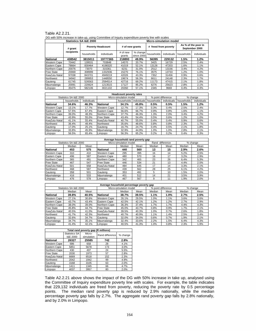
164
Table A2.2.21.
Table A2.2.21 above shows the impact of the DG with 50% increase in take up, analysed using the Committee of Inquiry expenditure poverty line with scales. For example, the table indicates that 229,132 individuals are freed from poverty, reducing the poverty rate by 0.5 percentage points. The median rand poverty gap is reduced by 2.9% nationally, while the median percentage poverty gap falls by 2.7%. The aggregate rand poverty gap falls by 2.8% nationally, and by 2.0% in Limpopo.
DG with 50% increase in take-up, using Committee of Inquiry expenditure poverty line with scales
households individuals # of new grants
% change since 2000 households individuals households individuals
National 438542 3815011 19777365 218893 49.9% 56395 229132 1.5% 1.2%Western Cape 70442 139531 703848 14570 20.7% 3425 16729 2.5% 2.4%Eastern Cape 78664 830464 4198320 41019 52.1% 13126 47203 1.6% 1.1%Northern Cape 20076 73070 315361 6231 31.0% 2512 13156 3.4% 4.2%Free State 20069 308999 1332936 15270 76.1% 3575 13733 1.2% 1.0%KwaZulu-Natal 97038 843701 4949219 42026 43.3% 7352 31456 0.9% 0.6%Northwest 34942 289953 1448550 19674 56.3% 6611 24148 2.3% 1.7%Gauteng 61745 526563 2594514 42716 69.2% 11173 47415 2.1% 1.8%Mpumalanga 20091 220624 1213515 17127 85.2% 6276 25623 2.8% 2.1%Limpopo 35475 582106 3021102 20260 57.1% 2345 9669 0.4% 0.3%
households individuals households individuals households individuals households individualsNational 34.6% 46.3% National 34.1% 45.8% 0.5% 0.5% 1.5% 1.2%Western Cape 13.1% 17.7% Western Cape 12.7% 17.3% 0.3% 0.4% 2.5% 2.4%Eastern Cape 57.5% 67.4% Eastern Cape 56.6% 66.7% 0.9% 0.8% 1.6% 1.1%Northern Cape 39.0% 48.3% Northern Cape 37.7% 46.3% 1.3% 2.0% 3.4% 4.2%Free State 43.9% 55.0% Free State 43.4% 54.4% 0.5% 0.6% 1.2% 1.0%KwaZulu-Natal 41.1% 55.4% KwaZulu-Natal 40.7% 55.0% 0.4% 0.4% 0.9% 0.6%Northwest 36.4% 49.4% Northwest 35.6% 48.6% 0.8% 0.8% 2.3% 1.7%Gauteng 17.0% 25.1% Gauteng 16.7% 24.7% 0.4% 0.5% 2.1% 1.8%Mpumalanga 33.8% 45.9% Mpumalanga 32.9% 44.9% 1.0% 1.0% 2.8% 2.1%Limpopo 56.5% 65.4% Limpopo 56.3% 65.2% 0.2% 0.2% 0.4% 0.3%
Median Mean Median Mean Median Mean Median MeanNational 453 575 National 440 560 13 15 2.9% 2.6%Western Cape 310 410 Western Cape 295 395 16 14 5.2% 3.5%Eastern Cape 496 587 Eastern Cape 480 570 16 17 3.2% 2.9%Northern Cape 365 491 Northern Cape 342 465 23 26 6.4% 5.3%Free State 467 547 Free State 446 534 21 13 4.4% 2.5%KwaZulu-Natal 501 658 KwaZulu-Natal 484 645 17 14 3.3% 2.1%Northwest 468 587 Northwest 439 562 28 25 6.1% 4.2%Gauteng 358 501 Gauteng 353 491 5 10 1.5% 2.0%Mpumalanga 416 533 Mpumalanga 401 512 14 21 3.5% 3.9%Limpopo 476 578 Limpopo 467 567 9 11 1.9% 2.0%
Median Mean Median Mean Median Mean Median MeanNational 39.8% 40.5% National 38.7% 39.5% 1.1% 1.0% 2.7% 2.5%Western Cape 27.1% 30.6% Western Cape 26.1% 29.5% 1.0% 1.1% 3.6% 3.6%Eastern Cape 43.7% 43.4% Eastern Cape 42.5% 42.1% 1.2% 1.2% 2.7% 2.9%Northern Cape 38.0% 39.0% Northern Cape 36.3% 37.4% 1.7% 1.7% 4.4% 4.3%Free State 45.8% 44.7% Free State 45.0% 43.7% 0.8% 0.9% 1.7% 2.1%KwaZulu-Natal 40.5% 41.0% KwaZulu-Natal 39.5% 40.3% 1.0% 0.7% 2.6% 1.8%Northwest 41.7% 42.3% Northwest 40.7% 40.9% 1.1% 1.4% 2.5% 3.4%Gauteng 32.6% 34.7% Gauteng 32.0% 34.0% 0.6% 0.7% 1.9% 2.1%Mpumalanga 34.7% 35.1% Mpumalanga 32.4% 33.6% 2.2% 1.5% 6.4% 4.3%Limpopo 41.4% 42.1% Limpopo 40.5% 41.3% 1.0% 0.8% 2.3% 1.9%
Statistics SA I&E 2000
Micro-simulation Rand difference % change
National 26327 25585 742 2.8%Western Cape 686 658 28 4.1%Eastern Cape 5851 5678 173 3.0%Northern Cape 430 407 24 5.5%Free State 2030 1973 57 2.8%KwaZulu-Natal 6669 6518 152 2.3%Northwest 2042 1942 99 4.9%Gauteng 3168 3105 63 2.0%Mpumalanga 1411 1345 66 4.7%Limpopo 4037 3957 80 2.0%
% change
Headcount poverty rates
# of new grants # freed from poverty As % of the poor in September 2000
Statistics SA I&E 2000 % point difference
Statistics SA I&E 2000 Micro-simulation model Rand differenceAverage household rand poverty gap
% change
% changeMicro-simulation model
Total rand poverty gap (R millions)
Statistics SA I&E 2000 Micro-simulation model
Micro-simulation modelStatistics SA I&E 2000
Poverty Headcount# grant
recipients
% point differenceAverage household percentage poverty gap

165
Table A2.2.22.
Table A2.2.22 above shows the impact of the DG with full take up, analysed using the Committee of Inquiry expenditure poverty line with scales. For example, the table indicates that 952,228 individuals are freed from poverty, reducing the poverty rate by 2.2 percentage points. The median rand poverty gap is reduced by 12.2% nationally, while the median percentage poverty gap falls by 10.5%. The aggregate rand poverty gap falls by 9.3% nationally, and by 7.4% in Limpopo.
DG with full take-up, using Committee of Inquiry expenditure poverty line with scales
households individuals # of new grants
% change since 2000 households individuals households individuals
National 438542 3815011 19777365 780318 177.9% 215066 952228 5.6% 4.8%Western Cape 70442 139531 703848 55546 78.9% 8657 39586 6.2% 5.6%Eastern Cape 78664 830464 4198320 150466 191.3% 51929 219090 6.3% 5.2%Northern Cape 20076 73070 315361 22818 113.7% 7251 31611 9.9% 10.0%Free State 20069 308999 1332936 54619 272.2% 15023 67337 4.9% 5.1%KwaZulu-Natal 97038 843701 4949219 158093 162.9% 37942 187611 4.5% 3.8%Northwest 34942 289953 1448550 74196 212.3% 23433 103272 8.1% 7.1%Gauteng 61745 526563 2594514 136145 220.5% 30890 130596 5.9% 5.0%Mpumalanga 20091 220624 1213515 52758 262.6% 15888 73641 7.2% 6.1%Limpopo 35475 582106 3021102 75677 213.3% 24053 99484 4.1% 3.3%
households individuals households individuals households individuals households individualsNational 34.6% 46.3% National 32.6% 44.1% 2.0% 2.2% 5.6% 4.8%Western Cape 13.1% 17.7% Western Cape 12.2% 16.7% 0.8% 1.0% 6.2% 5.6%Eastern Cape 57.5% 67.4% Eastern Cape 53.9% 63.9% 3.6% 3.5% 6.3% 5.2%Northern Cape 39.0% 48.3% Northern Cape 35.2% 43.5% 3.9% 4.8% 9.9% 10.0%Free State 43.9% 55.0% Free State 41.7% 52.2% 2.1% 2.8% 4.9% 5.1%KwaZulu-Natal 41.1% 55.4% KwaZulu-Natal 39.2% 53.3% 1.8% 2.1% 4.5% 3.8%Northwest 36.4% 49.4% Northwest 33.5% 45.9% 2.9% 3.5% 8.1% 7.1%Gauteng 17.0% 25.1% Gauteng 16.0% 23.9% 1.0% 1.3% 5.9% 5.0%Mpumalanga 33.8% 45.9% Mpumalanga 31.4% 43.1% 2.4% 2.8% 7.2% 6.1%Limpopo 56.5% 65.4% Limpopo 54.2% 63.2% 2.3% 2.2% 4.1% 3.3%
Median Mean Median Mean Median Mean Median MeanNational 453 575 National 398 522 55 53 12.2% 9.3%Western Cape 310 410 Western Cape 271 368 53 42 17.1% 10.2%Eastern Cape 496 587 Eastern Cape 443 530 53 57 10.7% 9.8%Northern Cape 365 491 Northern Cape 299 421 66 70 18.1% 14.3%Free State 467 547 Free State 404 500 63 47 13.6% 8.6%KwaZulu-Natal 501 658 KwaZulu-Natal 455 605 46 53 9.2% 8.0%Northwest 468 587 Northwest 381 506 87 81 18.6% 13.8%Gauteng 358 501 Gauteng 327 457 32 45 8.8% 8.9%Mpumalanga 416 533 Mpumalanga 370 473 46 60 11.1% 11.3%Limpopo 476 578 Limpopo 436 535 40 43 8.4% 7.4%
Median Mean Median Mean Median Mean Median MeanNational 39.8% 40.5% National 35.6% 36.8% 4.2% 3.7% 10.5% 9.1%Western Cape 27.1% 30.6% Western Cape 24.1% 27.7% 3.0% 2.9% 11.0% 9.4%Eastern Cape 43.7% 43.4% Eastern Cape 38.9% 39.2% 4.8% 4.2% 11.0% 9.7%Northern Cape 38.0% 39.0% Northern Cape 33.4% 34.0% 4.6% 5.1% 12.1% 13.0%Free State 45.8% 44.7% Free State 41.9% 41.2% 3.9% 3.5% 8.5% 7.8%KwaZulu-Natal 40.5% 41.0% KwaZulu-Natal 36.5% 37.7% 4.0% 3.3% 9.8% 8.1%Northwest 41.7% 42.3% Northwest 35.1% 36.7% 6.6% 5.6% 15.9% 13.1%Gauteng 32.6% 34.7% Gauteng 30.1% 31.7% 2.5% 3.0% 7.7% 8.8%Mpumalanga 34.7% 35.1% Mpumalanga 29.6% 31.3% 5.0% 3.7% 14.6% 10.6%Limpopo 41.4% 42.1% Limpopo 38.1% 38.9% 3.4% 3.2% 8.2% 7.6%
Statistics SA I&E 2000
Micro-simulation Rand difference % change
National 26327 23891 2436 9.3%Western Cape 686 616 70 10.2%Eastern Cape 5851 5280 571 9.8%Northern Cape 430 369 62 14.3%Free State 2030 1855 175 8.6%KwaZulu-Natal 6669 6133 536 8.0%Northwest 2042 1760 281 13.8%Gauteng 3168 2885 284 8.9%Mpumalanga 1411 1252 160 11.3%Limpopo 4037 3739 298 7.4%
% change
Headcount poverty rates
# of new grants # freed from poverty As % of the poor in September 2000
Statistics SA I&E 2000 % point difference
Statistics SA I&E 2000 Micro-simulation model Rand differenceAverage household rand poverty gap
% change
% changeMicro-simulation model
Total rand poverty gap (R millions)
Statistics SA I&E 2000 Micro-simulation model
Micro-simulation modelStatistics SA I&E 2000
Poverty Headcount# grant
recipients
% point differenceAverage household percentage poverty gap
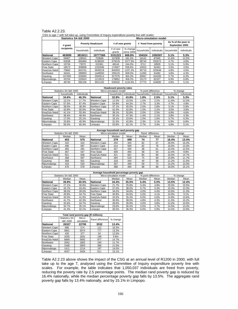
166
Table A2.2.23.
Table A2.2.23 above shows the impact of the CSG at an annual level of R1200 in 2000, with full take up to the age 7, analysed using the Committee of Inquiry expenditure poverty line with scales. For example, the table indicates that 1,050,037 individuals are freed from poverty, reducing the poverty rate by 2.5 percentage points. The median rand poverty gap is reduced by 16.4% nationally, while the median percentage poverty gap falls by 13.5%. The aggregate rand poverty gap falls by 13.4% nationally, and by 15.1% in Limpopo.
CSG to age 7 with full take-up, using Committee of Inquiry expenditure poverty line with scales
households individuals # of new grants
% change since 2000 households individuals households individuals
National 463699 3815011 19777365 3101223 668.8% 194324 1050307 5.1% 5.3%Western Cape 59407 139531 703848 107838 181.5% 16141 87845 11.6% 12.5%Eastern Cape 63038 830464 4198320 679216 1077.5% 38744 202672 4.7% 4.8%Northern Cape 19734 73070 315361 48144 244.0% 3712 18505 5.1% 5.9%Free State 18573 308999 1332936 174507 939.6% 10910 52463 3.5% 3.9%KwaZulu-Natal 70660 843701 4949219 845933 1197.2% 40715 225648 4.8% 4.6%Northwest 34341 289953 1448550 209125 609.0% 11092 61682 3.8% 4.3%Gauteng 107493 526563 2594514 327076 304.3% 30067 164335 5.7% 6.3%Mpumalanga 43704 220624 1213515 178852 409.2% 15173 82327 6.9% 6.8%Limpopo 46749 582106 3021102 530532 1134.9% 27770 154830 4.8% 5.1%
households individuals households individuals households individuals households individualsNational 34.6% 46.3% National 32.8% 43.8% 1.8% 2.5% 5.1% 5.3%Western Cape 13.1% 17.7% Western Cape 11.5% 15.5% 1.5% 2.2% 11.6% 12.5%Eastern Cape 57.5% 67.4% Eastern Cape 54.8% 64.2% 2.7% 3.3% 4.7% 4.8%Northern Cape 39.0% 48.3% Northern Cape 37.1% 45.5% 2.0% 2.8% 5.1% 5.9%Free State 43.9% 55.0% Free State 42.3% 52.8% 1.5% 2.2% 3.5% 3.9%KwaZulu-Natal 41.1% 55.4% KwaZulu-Natal 39.1% 52.8% 2.0% 2.5% 4.8% 4.6%Northwest 36.4% 49.4% Northwest 35.1% 47.3% 1.4% 2.1% 3.8% 4.3%Gauteng 17.0% 25.1% Gauteng 16.1% 23.6% 1.0% 1.6% 5.7% 6.3%Mpumalanga 33.8% 45.9% Mpumalanga 31.5% 42.8% 2.3% 3.1% 6.9% 6.8%Limpopo 56.5% 65.4% Limpopo 53.8% 62.1% 2.7% 3.4% 4.8% 5.1%
Median Mean Median Mean Median Mean Median MeanNational 453 575 National 379 498 74 77 16.4% 13.4%Western Cape 310 410 Western Cape 254 343 82 67 26.5% 16.3%Eastern Cape 496 587 Eastern Cape 414 509 82 78 16.6% 13.3%Northern Cape 365 491 Northern Cape 327 430 38 61 10.4% 12.5%Free State 467 547 Free State 409 494 58 54 12.4% 9.8%KwaZulu-Natal 501 658 KwaZulu-Natal 421 562 80 96 16.0% 14.7%Northwest 468 587 Northwest 394 518 74 69 15.8% 11.7%Gauteng 358 501 Gauteng 318 444 40 58 11.2% 11.5%Mpumalanga 416 533 Mpumalanga 357 459 59 74 14.2% 14.0%Limpopo 476 578 Limpopo 388 490 88 88 18.5% 15.1%
Median Mean Median Mean Median Mean Median MeanNational 39.8% 40.5% National 34.4% 35.5% 5.4% 5.0% 13.5% 12.4%Western Cape 27.1% 30.6% Western Cape 21.7% 25.8% 5.4% 4.8% 20.0% 15.5%Eastern Cape 43.7% 43.4% Eastern Cape 37.0% 38.0% 6.7% 5.4% 15.3% 12.3%Northern Cape 38.0% 39.0% Northern Cape 34.0% 34.6% 4.0% 4.4% 10.6% 11.3%Free State 45.8% 44.7% Free State 40.8% 40.6% 5.0% 4.1% 10.9% 9.1%KwaZulu-Natal 40.5% 41.0% KwaZulu-Natal 34.5% 35.4% 6.0% 5.6% 14.8% 13.6%Northwest 41.7% 42.3% Northwest 36.9% 38.0% 4.8% 4.3% 11.5% 10.2%Gauteng 32.6% 34.7% Gauteng 28.6% 30.9% 4.0% 3.8% 12.4% 10.9%Mpumalanga 34.7% 35.1% Mpumalanga 29.6% 30.4% 5.0% 4.7% 14.5% 13.3%Limpopo 41.4% 42.1% Limpopo 35.5% 36.3% 6.0% 5.9% 14.4% 13.9%
Statistics SA I&E 2000
Micro-simulation Rand difference % change
National 26327 22795 3532 13.4%Western Cape 686 574 112 16.3%Eastern Cape 5851 5074 777 13.3%Northern Cape 430 377 54 12.5%Free State 2030 1831 199 9.8%KwaZulu-Natal 6669 5692 977 14.7%Northwest 2042 1802 240 11.7%Gauteng 3168 2803 366 11.5%Mpumalanga 1411 1214 197 14.0%Limpopo 4037 3426 611 15.1%
Total rand poverty gap (R millions)
Statistics SA I&E 2000 Micro-simulation model
Micro-simulation modelStatistics SA I&E 2000
Poverty Headcount# grant
recipients
% point differenceAverage household percentage poverty gap
Average household rand poverty gap% change
% changeMicro-simulation model
% change
Headcount poverty rates
# of new grants # freed from poverty As % of the poor in September 2000
Statistics SA I&E 2000 % point difference
Statistics SA I&E 2000 Micro-simulation model Rand difference

167
Table A2.2.24.
Table A2.2.24 above shows the impact of the CSG at an annual level of R1200 in 2000, with full take up to the age 9, analysed using the Committee of Inquiry expenditure poverty line with scales. For example, the table indicates that 1,520,841 individuals are freed from poverty, reducing the poverty rate by 3.6 percentage points. The median rand poverty gap is reduced by 21.1% nationally, while the median percentage poverty gap falls by 17.5%. The aggregate rand poverty gap falls by 17.9% nationally, and by 20.0% in Limpopo.
CSG to age 9 with full take-up, using Committee of Inquiry expenditure poverty line with scales
households individuals # of new grants
% change since 2000 households individuals households individuals
National 463699 3815011 19777365 4171697 899.7% 277395 1520841 7.3% 7.7%Western Cape 59407 139531 703848 139948 235.6% 19930 113055 14.3% 16.1%Eastern Cape 63038 830464 4198320 925982 1468.9% 56026 299749 6.7% 7.1%Northern Cape 19734 73070 315361 60131 304.7% 4799 23938 6.6% 7.6%Free State 18573 308999 1332936 238089 1281.9% 15883 75289 5.1% 5.6%KwaZulu-Natal 70660 843701 4949219 1140500 1614.1% 61135 353017 7.2% 7.1%Northwest 34341 289953 1448550 285717 832.0% 17153 93778 5.9% 6.5%Gauteng 107493 526563 2594514 427550 397.7% 37049 206852 7.0% 8.0%Mpumalanga 43704 220624 1213515 247308 565.9% 23020 126083 10.4% 10.4%Limpopo 46749 582106 3021102 706472 1511.2% 42400 229080 7.3% 7.6%
households individuals households individuals households individuals households individualsNational 34.6% 46.3% National 32.1% 42.7% 2.5% 3.6% 7.3% 7.7%Western Cape 13.1% 17.7% Western Cape 11.2% 14.9% 1.9% 2.8% 14.3% 16.1%Eastern Cape 57.5% 67.4% Eastern Cape 53.6% 62.6% 3.9% 4.8% 6.7% 7.1%Northern Cape 39.0% 48.3% Northern Cape 36.5% 44.6% 2.6% 3.7% 6.6% 7.6%Free State 43.9% 55.0% Free State 41.6% 51.8% 2.3% 3.1% 5.1% 5.6%KwaZulu-Natal 41.1% 55.4% KwaZulu-Natal 38.1% 51.4% 3.0% 3.9% 7.2% 7.1%Northwest 36.4% 49.4% Northwest 34.3% 46.2% 2.2% 3.2% 5.9% 6.5%Gauteng 17.0% 25.1% Gauteng 15.8% 23.1% 1.2% 2.0% 7.0% 8.0%Mpumalanga 33.8% 45.9% Mpumalanga 30.3% 41.1% 3.5% 4.8% 10.4% 10.4%Limpopo 56.5% 65.4% Limpopo 52.4% 60.4% 4.1% 5.0% 7.3% 7.6%
Median Mean Median Mean Median Mean Median MeanNational 453 575 National 357 472 96 103 21.1% 17.9%Western Cape 310 410 Western Cape 246 325 111 84 36.0% 20.5%Eastern Cape 496 587 Eastern Cape 385 482 111 105 22.5% 17.9%Northern Cape 365 491 Northern Cape 311 415 54 76 14.8% 15.5%Free State 467 547 Free State 395 475 72 73 15.3% 13.3%KwaZulu-Natal 501 658 KwaZulu-Natal 395 530 106 128 21.2% 19.5%Northwest 468 587 Northwest 361 494 107 93 22.8% 15.9%Gauteng 358 501 Gauteng 304 426 54 75 15.1% 15.0%Mpumalanga 416 533 Mpumalanga 318 431 97 102 23.4% 19.1%Limpopo 476 578 Limpopo 365 463 112 115 23.4% 20.0%
Median Mean Median Mean Median Mean Median MeanNational 39.8% 40.5% National 32.8% 33.8% 7.0% 6.7% 17.5% 16.6%Western Cape 27.1% 30.6% Western Cape 20.4% 24.7% 6.6% 5.9% 24.5% 19.2%Eastern Cape 43.7% 43.4% Eastern Cape 35.1% 36.1% 8.6% 7.2% 19.7% 16.7%Northern Cape 38.0% 39.0% Northern Cape 33.0% 33.5% 5.1% 5.5% 13.3% 14.2%Free State 45.8% 44.7% Free State 39.8% 39.1% 6.0% 5.6% 13.1% 12.4%KwaZulu-Natal 40.5% 41.0% KwaZulu-Natal 32.9% 33.5% 7.6% 7.5% 18.7% 18.3%Northwest 41.7% 42.3% Northwest 35.3% 36.3% 6.4% 6.0% 15.4% 14.1%Gauteng 32.6% 34.7% Gauteng 27.8% 29.8% 4.8% 5.0% 14.7% 14.3%Mpumalanga 34.7% 35.1% Mpumalanga 27.7% 28.6% 6.9% 6.4% 20.0% 18.3%Limpopo 41.4% 42.1% Limpopo 33.2% 34.3% 8.2% 7.8% 19.9% 18.6%
Statistics SA I&E 2000
Micro-simulation Rand difference % change
National 26327 21627 4700 17.9%Western Cape 686 545 141 20.5%Eastern Cape 5851 4801 1049 17.9%Northern Cape 430 364 67 15.5%Free State 2030 1761 269 13.3%KwaZulu-Natal 6669 5372 1298 19.5%Northwest 2042 1718 324 15.9%Gauteng 3168 2692 476 15.0%Mpumalanga 1411 1141 270 19.1%Limpopo 4037 3231 806 20.0%
Total rand poverty gap (R millions)
Statistics SA I&E 2000 Micro-simulation model
Micro-simulation modelStatistics SA I&E 2000
Poverty Headcount# grant
recipients
% point differenceAverage household percentage poverty gap
Average household rand poverty gap% change
% changeMicro-simulation model
% change
Headcount poverty rates
# of new grants # freed from poverty As % of the poor in September 2000
Statistics SA I&E 2000 % point difference
Statistics SA I&E 2000 Micro-simulation model Rand difference

168
Table A2.2.25.
Table A2.2.25 above shows the impact of the CSG at an annual level of R1200 in 2000, with full take up to the age 11, analysed using the Committee of Inquiry expenditure poverty line with scales. For example, the table indicates that 1,941,408 individuals are freed from poverty, reducing the poverty rate by 4.5 percentage points. The median rand poverty gap is reduced by 25.9% nationally, while the median percentage poverty gap falls by 22.8%. The aggregate rand poverty gap falls by 22.4% nationally, and by 25.0% in Limpopo.
CSG to age 11 with full take-up, using Committee of Inquiry expenditure poverty line with scales
households individuals # of new grants
% change since 2000 households individuals households individuals
National 463699 3815011 19777365 5285914 1139.9% 355624 1941408 9.3% 9.8%Western Cape 59407 139531 703848 180280 303.5% 25397 140854 18.2% 20.0%Eastern Cape 63038 830464 4198320 1188951 1886.1% 71595 387482 8.6% 9.2%Northern Cape 19734 73070 315361 74935 379.7% 5974 30964 8.2% 9.8%Free State 18573 308999 1332936 307372 1654.9% 20886 97004 6.8% 7.3%KwaZulu-Natal 70660 843701 4949219 1420667 2010.6% 78172 438559 9.3% 8.9%Northwest 34341 289953 1448550 364967 1062.8% 23554 131910 8.1% 9.1%Gauteng 107493 526563 2594514 534330 497.1% 46515 259528 8.8% 10.0%Mpumalanga 43704 220624 1213515 313703 717.8% 29042 160185 13.2% 13.2%Limpopo 46749 582106 3021102 900709 1926.7% 54489 294922 9.4% 9.8%
households individuals households individuals households individuals households individualsNational 34.6% 46.3% National 31.4% 41.7% 3.2% 4.5% 9.3% 9.8%Western Cape 13.1% 17.7% Western Cape 10.7% 14.2% 2.4% 3.6% 18.2% 20.0%Eastern Cape 57.5% 67.4% Eastern Cape 52.6% 61.2% 5.0% 6.2% 8.6% 9.2%Northern Cape 39.0% 48.3% Northern Cape 35.9% 43.6% 3.2% 4.7% 8.2% 9.8%Free State 43.9% 55.0% Free State 40.9% 51.0% 3.0% 4.0% 6.8% 7.3%KwaZulu-Natal 41.1% 55.4% KwaZulu-Natal 37.3% 50.5% 3.8% 4.9% 9.3% 8.9%Northwest 36.4% 49.4% Northwest 33.5% 44.9% 3.0% 4.5% 8.1% 9.1%Gauteng 17.0% 25.1% Gauteng 15.5% 22.6% 1.5% 2.5% 8.8% 10.0%Mpumalanga 33.8% 45.9% Mpumalanga 29.4% 39.8% 4.5% 6.1% 13.2% 13.2%Limpopo 56.5% 65.4% Limpopo 51.2% 59.0% 5.3% 6.4% 9.4% 9.8%
Median Mean Median Mean Median Mean Median MeanNational 453 575 National 336 446 118 129 25.9% 22.4%Western Cape 310 410 Western Cape 202 303 132 107 42.7% 26.0%Eastern Cape 496 587 Eastern Cape 364 453 132 134 26.7% 22.9%Northern Cape 365 491 Northern Cape 293 398 72 93 19.8% 19.0%Free State 467 547 Free State 373 454 95 94 20.2% 17.1%KwaZulu-Natal 501 658 KwaZulu-Natal 366 500 135 158 27.0% 24.0%Northwest 468 587 Northwest 347 469 121 118 25.8% 20.1%Gauteng 358 501 Gauteng 284 409 75 93 20.8% 18.5%Mpumalanga 416 533 Mpumalanga 300 405 116 128 27.9% 24.0%Limpopo 476 578 Limpopo 330 433 147 145 30.8% 25.0%
Median Mean Median Mean Median Mean Median MeanNational 39.8% 40.5% National 30.7% 32.1% 9.1% 8.4% 22.8% 20.7%Western Cape 27.1% 30.6% Western Cape 18.2% 23.1% 8.9% 7.5% 32.9% 24.5%Eastern Cape 43.7% 43.4% Eastern Cape 32.5% 34.2% 11.2% 9.2% 25.6% 21.2%Northern Cape 38.0% 39.0% Northern Cape 31.9% 32.3% 6.1% 6.7% 16.1% 17.2%Free State 45.8% 44.7% Free State 37.9% 37.6% 8.0% 7.1% 17.4% 15.9%KwaZulu-Natal 40.5% 41.0% KwaZulu-Natal 30.2% 31.8% 10.4% 9.2% 25.6% 22.5%Northwest 41.7% 42.3% Northwest 33.8% 34.8% 8.0% 7.5% 19.1% 17.8%Gauteng 32.6% 34.7% Gauteng 26.5% 28.7% 6.1% 6.0% 18.7% 17.2%Mpumalanga 34.7% 35.1% Mpumalanga 25.6% 27.0% 9.1% 8.1% 26.1% 23.0%Limpopo 41.4% 42.1% Limpopo 31.1% 32.3% 10.3% 9.9% 24.9% 23.4%
Statistics SA I&E 2000
Micro-simulation Rand difference % change
National 26327 20434 5893 22.4%Western Cape 686 507 178 26.0%Eastern Cape 5851 4514 1337 22.9%Northern Cape 430 349 82 19.0%Free State 2030 1683 347 17.1%KwaZulu-Natal 6669 5066 1604 24.0%Northwest 2042 1632 409 20.1%Gauteng 3168 2583 585 18.5%Mpumalanga 1411 1072 339 24.0%Limpopo 4037 3026 1011 25.0%
Total rand poverty gap (R millions)
Statistics SA I&E 2000 Micro-simulation model
Micro-simulation modelStatistics SA I&E 2000
Poverty Headcount# grant
recipients
% point differenceAverage household percentage poverty gap
Average household rand poverty gap% change
% changeMicro-simulation model
% change
Headcount poverty rates
# of new grants # freed from poverty As % of the poor in September 2000
Statistics SA I&E 2000 % point difference
Statistics SA I&E 2000 Micro-simulation model Rand difference

169
Table A2.2.26.
Table A2.2.26 above shows the impact of the CSG at an annual level of R1200 in 2000, with full take up to the age 14, analysed using the Committee of Inquiry expenditure poverty line with scales. For example, the table indicates that 2,654,378 individuals are freed from poverty, reducing the poverty rate by 6.2 percentage points. The median rand poverty gap is reduced by 33.3% nationally, while the median percentage poverty gap falls by 30.4%. The aggregate rand poverty gap falls by 28.8% nationally, and by 32.4% in Limpopo.
CSG to age 14 with full take-up, using Committee of Inquiry expenditure poverty line with scales
households individuals # of new grants
% change since 2000 households individuals households individuals
National 463699 3815011 19777365 6913218 1490.9% 483619 2654378 12.7% 13.4%Western Cape 59407 139531 703848 222955 375.3% 31084 176438 22.3% 25.1%Eastern Cape 63038 830464 4198320 1583364 2511.8% 101321 544893 12.2% 13.0%Northern Cape 19734 73070 315361 94693 479.8% 7781 39845 10.6% 12.6%Free State 18573 308999 1332936 401927 2164.0% 25956 120158 8.4% 9.0%KwaZulu-Natal 70660 843701 4949219 1834931 2596.8% 104668 590024 12.4% 11.9%Northwest 34341 289953 1448550 483087 1406.7% 33914 192006 11.7% 13.3%Gauteng 107493 526563 2594514 691901 643.7% 61093 356960 11.6% 13.8%Mpumalanga 43704 220624 1213515 415348 950.4% 39491 220097 17.9% 18.1%Limpopo 46749 582106 3021102 1185012 2534.8% 78311 413957 13.5% 13.7%
households individuals households individuals households individuals households individualsNational 34.6% 46.3% National 30.2% 40.1% 4.4% 6.2% 12.7% 13.4%Western Cape 13.1% 17.7% Western Cape 10.1% 13.3% 2.9% 4.4% 22.3% 25.1%Eastern Cape 57.5% 67.4% Eastern Cape 50.5% 58.7% 7.0% 8.8% 12.2% 13.0%Northern Cape 39.0% 48.3% Northern Cape 34.9% 42.2% 4.2% 6.1% 10.6% 12.6%Free State 43.9% 55.0% Free State 40.2% 50.0% 3.7% 5.0% 8.4% 9.0%KwaZulu-Natal 41.1% 55.4% KwaZulu-Natal 36.0% 48.8% 5.1% 6.6% 12.4% 11.9%Northwest 36.4% 49.4% Northwest 32.2% 42.9% 4.3% 6.5% 11.7% 13.3%Gauteng 17.0% 25.1% Gauteng 15.1% 21.7% 2.0% 3.5% 11.6% 13.8%Mpumalanga 33.8% 45.9% Mpumalanga 27.8% 37.6% 6.1% 8.3% 17.9% 18.1%Limpopo 56.5% 65.4% Limpopo 48.9% 56.4% 7.6% 9.0% 13.5% 13.7%
Median Mean Median Mean Median Mean Median MeanNational 453 575 National 302 410 151 165 33.3% 28.8%Western Cape 310 410 Western Cape 171 281 175 128 56.5% 31.3%Eastern Cape 496 587 Eastern Cape 321 412 175 175 35.3% 29.8%Northern Cape 365 491 Northern Cape 287 374 78 117 21.4% 23.8%Free State 467 547 Free State 339 426 128 121 27.4% 22.2%KwaZulu-Natal 501 658 KwaZulu-Natal 325 457 176 201 35.1% 30.5%Northwest 468 587 Northwest 322 433 146 154 31.2% 26.2%Gauteng 358 501 Gauteng 263 383 96 118 26.7% 23.5%Mpumalanga 416 533 Mpumalanga 270 368 145 165 34.9% 30.9%Limpopo 476 578 Limpopo 285 391 192 187 40.2% 32.4%
Median Mean Median Mean Median Mean Median MeanNational 39.8% 40.5% National 27.7% 29.7% 12.1% 10.8% 30.4% 26.7%Western Cape 27.1% 30.6% Western Cape 17.0% 21.6% 10.1% 9.0% 37.1% 29.4%Eastern Cape 43.7% 43.4% Eastern Cape 29.1% 31.3% 14.6% 12.1% 33.3% 27.8%Northern Cape 38.0% 39.0% Northern Cape 29.3% 30.7% 8.7% 8.3% 22.9% 21.3%Free State 45.8% 44.7% Free State 34.9% 35.5% 10.9% 9.2% 23.8% 20.5%KwaZulu-Natal 40.5% 41.0% KwaZulu-Natal 27.5% 29.2% 13.0% 11.8% 32.2% 28.7%Northwest 41.7% 42.3% Northwest 30.7% 32.4% 11.0% 9.9% 26.5% 23.4%Gauteng 32.6% 34.7% Gauteng 24.9% 27.3% 7.7% 7.5% 23.7% 21.5%Mpumalanga 34.7% 35.1% Mpumalanga 22.2% 24.7% 12.5% 10.3% 35.9% 29.5%Limpopo 41.4% 42.1% Limpopo 27.6% 29.2% 13.9% 12.9% 33.4% 30.6%
Statistics SA I&E 2000
Micro-simulation Rand difference % change
National 26327 18755 7572 28.8%Western Cape 686 471 215 31.3%Eastern Cape 5851 4108 1743 29.8%Northern Cape 430 328 102 23.8%Free State 2030 1580 450 22.2%KwaZulu-Natal 6669 4634 2036 30.5%Northwest 2042 1507 535 26.2%Gauteng 3168 2422 746 23.5%Mpumalanga 1411 975 436 30.9%Limpopo 4037 2728 1309 32.4%
Total rand poverty gap (R millions)
Statistics SA I&E 2000 Micro-simulation model
Micro-simulation modelStatistics SA I&E 2000
Poverty Headcount# grant
recipients
% point differenceAverage household percentage poverty gap
Average household rand poverty gap% change
% changeMicro-simulation model
% change
Headcount poverty rates
# of new grants # freed from poverty As % of the poor in September 2000
Statistics SA I&E 2000 % point difference
Statistics SA I&E 2000 Micro-simulation model Rand difference
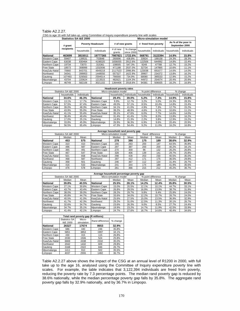
170
Table A2.2.27.
Table A2.2.27 above shows the impact of the CSG at an annual level of R1200 in 2000, with full take up to the age 16, analysed using the Committee of Inquiry expenditure poverty line with scales. For example, the table indicates that 3,122,394 individuals are freed from poverty, reducing the poverty rate by 7.3 percentage points. The median rand poverty gap is reduced by 38.6% nationally, while the median percentage poverty gap falls by 35.8%. The aggregate rand poverty gap falls by 32.9% nationally, and by 36.7% in Limpopo.
CSG to age 16 with full take-up, using Committee of Inquiry expenditure poverty line with scales
households individuals # of new grants
% change since 2000 households individuals households individuals
National 463699 3815011 19777365 7987821 1722.6% 568791 3122394 14.9% 15.8%Western Cape 59407 139531 703848 260696 438.8% 33924 199158 24.3% 28.3%Eastern Cape 63038 830464 4198320 1836055 2912.6% 122506 644992 14.8% 15.4%Northern Cape 19734 73070 315361 108005 547.3% 9249 47788 12.7% 15.2%Free State 18573 308999 1332936 471188 2537.0% 32734 147865 10.6% 11.1%KwaZulu-Natal 70660 843701 4949219 2117523 2996.8% 123038 691677 14.6% 14.0%Northwest 34341 289953 1448550 557327 1622.9% 39907 234372 13.8% 16.2%Gauteng 107493 526563 2594514 790000 734.9% 68080 395533 12.9% 15.2%Mpumalanga 43704 220624 1213515 482621 1104.3% 44972 254074 20.4% 20.9%Limpopo 46749 582106 3021102 1364406 2918.6% 94381 506935 16.2% 16.8%
households individuals households individuals households individuals households individualsNational 34.6% 46.3% National 29.4% 39.0% 5.2% 7.3% 14.9% 15.8%Western Cape 13.1% 17.7% Western Cape 9.9% 12.7% 3.2% 5.0% 24.3% 28.3%Eastern Cape 57.5% 67.4% Eastern Cape 49.0% 57.1% 8.5% 10.4% 14.8% 15.4%Northern Cape 39.0% 48.3% Northern Cape 34.1% 41.0% 4.9% 7.3% 12.7% 15.2%Free State 43.9% 55.0% Free State 39.2% 48.9% 4.6% 6.1% 10.6% 11.1%KwaZulu-Natal 41.1% 55.4% KwaZulu-Natal 35.1% 47.6% 6.0% 7.7% 14.6% 14.0%Northwest 36.4% 49.4% Northwest 31.4% 41.4% 5.0% 8.0% 13.8% 16.2%Gauteng 17.0% 25.1% Gauteng 14.8% 21.3% 2.2% 3.8% 12.9% 15.2%Mpumalanga 33.8% 45.9% Mpumalanga 26.9% 36.3% 6.9% 9.6% 20.4% 20.9%Limpopo 56.5% 65.4% Limpopo 47.3% 54.4% 9.2% 11.0% 16.2% 16.8%
Median Mean Median Mean Median Mean Median MeanNational 453 575 National 278 386 175 189 38.6% 32.9%Western Cape 310 410 Western Cape 156 263 200 147 64.5% 35.8%Eastern Cape 496 587 Eastern Cape 297 387 200 200 40.2% 34.1%Northern Cape 365 491 Northern Cape 270 359 96 132 26.2% 26.8%Free State 467 547 Free State 328 406 139 141 29.7% 25.8%KwaZulu-Natal 501 658 KwaZulu-Natal 298 428 203 230 40.5% 35.0%Northwest 468 587 Northwest 297 412 171 175 36.5% 29.8%Gauteng 358 501 Gauteng 246 367 112 134 31.4% 26.7%Mpumalanga 416 533 Mpumalanga 241 344 174 189 41.9% 35.5%Limpopo 476 578 Limpopo 261 366 215 212 45.2% 36.7%
Median Mean Median Mean Median Mean Median MeanNational 39.8% 40.5% National 25.5% 28.1% 14.2% 12.4% 35.8% 30.5%Western Cape 27.1% 30.6% Western Cape 15.0% 20.5% 12.1% 10.1% 44.7% 33.1%Eastern Cape 43.7% 43.4% Eastern Cape 26.8% 29.5% 16.9% 13.9% 38.7% 31.9%Northern Cape 38.0% 39.0% Northern Cape 28.2% 29.7% 9.8% 9.4% 25.9% 24.0%Free State 45.8% 44.7% Free State 33.6% 34.0% 12.2% 10.7% 26.7% 24.0%KwaZulu-Natal 40.5% 41.0% KwaZulu-Natal 25.6% 27.5% 15.0% 13.5% 36.9% 32.9%Northwest 41.7% 42.3% Northwest 29.2% 31.0% 12.5% 11.3% 30.1% 26.7%Gauteng 32.6% 34.7% Gauteng 23.6% 26.3% 9.0% 8.5% 27.7% 24.4%Mpumalanga 34.7% 35.1% Mpumalanga 19.9% 23.2% 14.7% 11.9% 42.5% 33.9%Limpopo 41.4% 42.1% Limpopo 24.7% 27.6% 16.7% 14.6% 40.4% 34.6%
Statistics SA I&E 2000
Micro-simulation Rand difference % change
National 26327 17674 8653 32.9%Western Cape 686 440 246 35.8%Eastern Cape 5851 3853 1997 34.1%Northern Cape 430 315 115 26.8%Free State 2030 1506 524 25.8%KwaZulu-Natal 6669 4338 2332 35.0%Northwest 2042 1432 609 29.8%Gauteng 3168 2322 846 26.7%Mpumalanga 1411 910 502 35.5%Limpopo 4037 2555 1482 36.7%
Total rand poverty gap (R millions)
Statistics SA I&E 2000 Micro-simulation model
Micro-simulation modelStatistics SA I&E 2000
Poverty Headcount# grant
recipients
% point differenceAverage household percentage poverty gap
Average household rand poverty gap% change
% changeMicro-simulation model
% change
Headcount poverty rates
# of new grants # freed from poverty As % of the poor in September 2000
Statistics SA I&E 2000 % point difference
Statistics SA I&E 2000 Micro-simulation model Rand difference
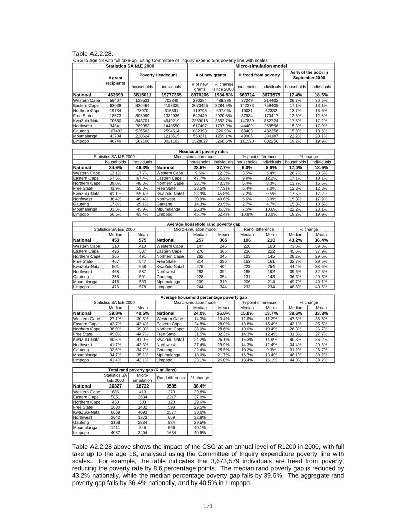
171
Table A2.2.28.
Table A2.2.28 above shows the impact of the CSG at an annual level of R1200 in 2000, with full take up to the age 18, analysed using the Committee of Inquiry expenditure poverty line with scales. For example, the table indicates that 3,673,579 individuals are freed from poverty, reducing the poverty rate by 8.6 percentage points. The median rand poverty gap is reduced by 43.2% nationally, while the median percentage poverty gap falls by 39.6%. The aggregate rand poverty gap falls by 36.4% nationally, and by 40.5% in Limpopo.
CSG to age 18 with full take-up, using Committee of Inquiry expenditure poverty line with scales
households individuals # of new grants
% change since 2000 households individuals households individuals
National 463699 3815011 19777365 8970206 1934.5% 663714 3673579 17.4% 18.6%Western Cape 59407 139531 703848 290394 488.8% 37249 214402 26.7% 30.5%Eastern Cape 63038 830464 4198320 2070456 3284.5% 142273 759409 17.1% 18.1%Northern Cape 19734 73070 315361 119795 607.0% 10031 52332 13.7% 16.6%Free State 18573 308999 1332936 542440 2920.6% 37934 170417 12.3% 12.8%KwaZulu-Natal 70660 843701 4949219 2369018 3352.7% 147839 852724 17.5% 17.2%Northwest 34341 289953 1448550 617407 1797.9% 44489 259596 15.3% 17.9%Gauteng 107493 526563 2594514 882398 820.9% 83403 482256 15.8% 18.6%Mpumalanga 43704 220624 1213515 550271 1259.1% 48906 280187 22.2% 23.1%Limpopo 46749 582106 3021102 1528027 3268.6% 111590 602256 19.2% 19.9%
households individuals households individuals households individuals households individualsNational 34.6% 46.3% National 28.6% 37.7% 6.0% 8.6% 17.4% 18.6%Western Cape 13.1% 17.7% Western Cape 9.6% 12.3% 3.5% 5.4% 26.7% 30.5%Eastern Cape 57.5% 67.4% Eastern Cape 47.7% 55.2% 9.9% 12.2% 17.1% 18.1%Northern Cape 39.0% 48.3% Northern Cape 33.7% 40.3% 5.4% 8.0% 13.7% 16.6%Free State 43.9% 55.0% Free State 38.5% 47.9% 5.4% 7.0% 12.3% 12.8%KwaZulu-Natal 41.1% 55.4% KwaZulu-Natal 33.9% 45.8% 7.2% 9.5% 17.5% 17.2%Northwest 36.4% 49.4% Northwest 30.9% 40.6% 5.6% 8.9% 15.3% 17.9%Gauteng 17.0% 25.1% Gauteng 14.3% 20.5% 2.7% 4.7% 15.8% 18.6%Mpumalanga 33.8% 45.9% Mpumalanga 26.3% 35.3% 7.5% 10.6% 22.2% 23.1%Limpopo 56.5% 65.4% Limpopo 45.7% 52.4% 10.8% 13.0% 19.2% 19.9%
Median Mean Median Mean Median Mean Median MeanNational 453 575 National 257 365 196 210 43.2% 36.4%Western Cape 310 410 Western Cape 147 246 226 163 73.0% 39.8%Eastern Cape 496 587 Eastern Cape 270 365 226 222 45.6% 37.9%Northern Cape 365 491 Northern Cape 262 345 103 145 28.2% 29.6%Free State 467 547 Free State 314 386 153 161 32.7% 29.5%KwaZulu-Natal 501 658 KwaZulu-Natal 279 404 222 254 44.4% 38.6%Northwest 468 587 Northwest 283 394 185 192 39.6% 32.8%Gauteng 358 501 Gauteng 228 354 131 148 36.5% 29.5%Mpumalanga 416 533 Mpumalanga 209 319 206 214 49.7% 40.1%Limpopo 476 578 Limpopo 244 344 233 234 48.8% 40.5%
Median Mean Median Mean Median Mean Median MeanNational 39.8% 40.5% National 24.0% 26.8% 15.8% 13.7% 39.6% 33.8%Western Cape 27.1% 30.6% Western Cape 14.3% 19.4% 12.8% 11.2% 47.3% 36.6%Eastern Cape 43.7% 43.4% Eastern Cape 24.8% 28.0% 18.8% 15.4% 43.1% 35.5%Northern Cape 38.0% 39.0% Northern Cape 28.0% 28.6% 10.0% 10.4% 26.3% 26.7%Free State 45.8% 44.7% Free State 31.5% 32.3% 14.3% 12.4% 31.3% 27.7%KwaZulu-Natal 40.5% 41.0% KwaZulu-Natal 24.2% 26.1% 16.3% 14.9% 40.3% 36.2%Northwest 41.7% 42.3% Northwest 27.4% 29.9% 14.3% 12.4% 34.4% 29.3%Gauteng 32.6% 34.7% Gauteng 22.4% 25.5% 10.2% 9.3% 31.2% 26.7%Mpumalanga 34.7% 35.1% Mpumalanga 18.0% 21.7% 16.7% 13.4% 48.1% 38.2%Limpopo 41.4% 42.1% Limpopo 23.1% 26.0% 18.4% 16.1% 44.3% 38.2%
Statistics SA I&E 2000
Micro-simulation Rand difference % change
National 26327 16732 9595 36.4%Western Cape 686 413 273 39.8%Eastern Cape 5851 3634 2217 37.9%Northern Cape 430 303 128 29.6%Free State 2030 1432 598 29.5%KwaZulu-Natal 6669 4093 2577 38.6%Northwest 2042 1373 669 32.8%Gauteng 3168 2234 934 29.5%Mpumalanga 1411 845 566 40.1%Limpopo 4037 2404 1634 40.5%
Total rand poverty gap (R millions)
Statistics SA I&E 2000 Micro-simulation model
Micro-simulation modelStatistics SA I&E 2000
Poverty Headcount# grant
recipients
% point differenceAverage household percentage poverty gap
Average household rand poverty gap% change
% changeMicro-simulation model
% change
Headcount poverty rates
# of new grants # freed from poverty As % of the poor in September 2000
Statistics SA I&E 2000 % point difference
Statistics SA I&E 2000 Micro-simulation model Rand difference

172
Table A2.2.29.
Table A2.2.29 above shows the impact of the CSG at an annual level of R1606 in 2000, with full take up to the age 7, analysed using the Committee of Inquiry expenditure poverty line with scales. For example, the table indicates that 1,466,285 individuals are freed from poverty, reducing the poverty rate by 3.4 percentage points. The median rand poverty gap is reduced by 21.8% nationally, while the median percentage poverty gap falls by 18.1%. The aggregate rand poverty gap falls by 17.6% nationally, and by 19.9% in Limpopo.
CSG(1606) to age 7 with full take-up, using Committee of Inquiry expenditure poverty line with scales
households individuals # of new grants
% change since 2000 households individuals households individuals
National 463699 3815011 19777365 3101223 668.8% 265691 1466285 7.0% 7.4%Western Cape 59407 139531 703848 107838 181.5% 20493 110721 14.7% 15.7%Eastern Cape 63038 830464 4198320 679216 1077.5% 50667 271417 6.1% 6.5%Northern Cape 19734 73070 315361 48144 244.0% 6037 29152 8.3% 9.2%Free State 18573 308999 1332936 174507 939.6% 13679 65997 4.4% 5.0%KwaZulu-Natal 70660 843701 4949219 845933 1197.2% 52597 297437 6.2% 6.0%Northwest 34341 289953 1448550 209125 609.0% 16802 101114 5.8% 7.0%Gauteng 107493 526563 2594514 327076 304.3% 43951 244300 8.3% 9.4%Mpumalanga 43704 220624 1213515 178852 409.2% 21548 120748 9.8% 10.0%Limpopo 46749 582106 3021102 530532 1134.9% 39917 225399 6.9% 7.5%
households individuals households individuals households individuals households individualsNational 34.6% 46.3% National 32.2% 42.9% 2.4% 3.4% 7.0% 7.4%Western Cape 13.1% 17.7% Western Cape 11.1% 15.0% 1.9% 2.8% 14.7% 15.7%Eastern Cape 57.5% 67.4% Eastern Cape 54.0% 63.1% 3.5% 4.4% 6.1% 6.5%Northern Cape 39.0% 48.3% Northern Cape 35.8% 43.8% 3.2% 4.5% 8.3% 9.2%Free State 43.9% 55.0% Free State 41.9% 52.2% 1.9% 2.7% 4.4% 5.0%KwaZulu-Natal 41.1% 55.4% KwaZulu-Natal 38.5% 52.0% 2.6% 3.3% 6.2% 6.0%Northwest 36.4% 49.4% Northwest 34.3% 46.0% 2.1% 3.4% 5.8% 7.0%Gauteng 17.0% 25.1% Gauteng 15.6% 22.8% 1.4% 2.4% 8.3% 9.4%Mpumalanga 33.8% 45.9% Mpumalanga 30.5% 41.3% 3.3% 4.6% 9.8% 10.0%Limpopo 56.5% 65.4% Limpopo 52.6% 60.5% 3.9% 4.9% 6.9% 7.5%
Median Mean Median Mean Median Mean Median MeanNational 453 575 National 354 474 99 101 21.8% 17.6%Western Cape 310 410 Western Cape 246 325 111 85 35.7% 20.8%Eastern Cape 496 587 Eastern Cape 386 485 111 103 22.3% 17.5%Northern Cape 365 491 Northern Cape 308 411 57 79 15.6% 16.2%Free State 467 547 Free State 392 477 75 71 16.2% 12.9%KwaZulu-Natal 501 658 KwaZulu-Natal 393 531 108 127 21.6% 19.3%Northwest 468 587 Northwest 382 496 86 91 18.4% 15.4%Gauteng 358 501 Gauteng 305 426 54 75 15.0% 15.0%Mpumalanga 416 533 Mpumalanga 333 436 83 97 19.9% 18.2%Limpopo 476 578 Limpopo 354 463 122 115 25.7% 19.9%
Median Mean Median Mean Median Mean Median MeanNational 39.8% 40.5% National 32.6% 33.9% 7.2% 6.5% 18.1% 16.1%Western Cape 27.1% 30.6% Western Cape 20.1% 24.6% 6.9% 6.0% 25.6% 19.6%Eastern Cape 43.7% 43.4% Eastern Cape 34.9% 36.4% 8.8% 7.0% 20.1% 16.2%Northern Cape 38.0% 39.0% Northern Cape 33.0% 33.3% 5.1% 5.7% 13.3% 14.6%Free State 45.8% 44.7% Free State 39.6% 39.4% 6.2% 5.3% 13.6% 11.9%KwaZulu-Natal 40.5% 41.0% KwaZulu-Natal 32.5% 33.7% 8.0% 7.3% 19.7% 17.9%Northwest 41.7% 42.3% Northwest 35.0% 36.6% 6.7% 5.7% 16.0% 13.4%Gauteng 32.6% 34.7% Gauteng 27.6% 29.8% 5.0% 4.9% 15.3% 14.1%Mpumalanga 34.7% 35.1% Mpumalanga 28.5% 29.0% 6.2% 6.0% 17.9% 17.2%Limpopo 41.4% 42.1% Limpopo 32.9% 34.5% 8.5% 7.7% 20.6% 18.2%
Statistics SA I&E 2000
Micro-simulation Rand difference % change
National 26327 21696 4631 17.6%Western Cape 686 543 142 20.8%Eastern Cape 5851 4829 1022 17.5%Northern Cape 430 361 70 16.2%Free State 2030 1768 262 12.9%KwaZulu-Natal 6669 5383 1287 19.3%Northwest 2042 1727 315 15.4%Gauteng 3168 2694 474 15.0%Mpumalanga 1411 1155 257 18.2%Limpopo 4037 3234 803 19.9%
Total rand poverty gap (R millions)
Statistics SA I&E 2000 Micro-simulation model
Micro-simulation modelStatistics SA I&E 2000
Poverty Headcount# grant
recipients
% point differenceAverage household percentage poverty gap
Average household rand poverty gap% change
% changeMicro-simulation model
% change
Headcount poverty rates
# of new grants # freed from poverty As % of the poor in September 2000
Statistics SA I&E 2000 % point difference
Statistics SA I&E 2000 Micro-simulation model Rand difference
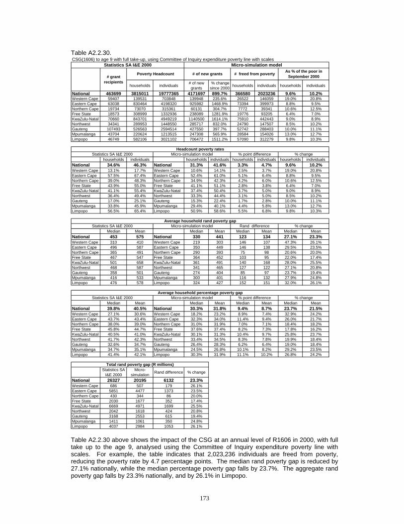
173
Table A2.2.30.
Table A2.2.30 above shows the impact of the CSG at an annual level of R1606 in 2000, with full take up to the age 9, analysed using the Committee of Inquiry expenditure poverty line with scales. For example, the table indicates that 2,023,236 individuals are freed from poverty, reducing the poverty rate by 4.7 percentage points. The median rand poverty gap is reduced by 27.1% nationally, while the median percentage poverty gap falls by 23.7%. The aggregate rand poverty gap falls by 23.3% nationally, and by 26.1% in Limpopo.
CSG(1606) to age 9 with full take-up, using Committee of Inquiry expenditure poverty line with scales
households individuals # of new grants
% change since 2000 households individuals households individuals
National 463699 3815011 19777365 4171697 899.7% 366580 2023236 9.6% 10.2%Western Cape 59407 139531 703848 139948 235.6% 26522 146059 19.0% 20.8%Eastern Cape 63038 830464 4198320 925982 1468.9% 73394 399973 8.8% 9.5%Northern Cape 19734 73070 315361 60131 304.7% 7772 39341 10.6% 12.5%Free State 18573 308999 1332936 238089 1281.9% 19776 93205 6.4% 7.0%KwaZulu-Natal 70660 843701 4949219 1140500 1614.1% 75910 442443 9.0% 8.9%Northwest 34341 289953 1448550 285717 832.0% 24790 147507 8.5% 10.2%Gauteng 107493 526563 2594514 427550 397.7% 52742 288403 10.0% 11.1%Mpumalanga 43704 220624 1213515 247308 565.9% 28584 154026 13.0% 12.7%Limpopo 46749 582106 3021102 706472 1511.2% 57090 312279 9.8% 10.3%
households individuals households individuals households individuals households individualsNational 34.6% 46.3% National 31.3% 41.6% 3.3% 4.7% 9.6% 10.2%Western Cape 13.1% 17.7% Western Cape 10.6% 14.1% 2.5% 3.7% 19.0% 20.8%Eastern Cape 57.5% 67.4% Eastern Cape 52.4% 61.0% 5.1% 6.4% 8.8% 9.5%Northern Cape 39.0% 48.3% Northern Cape 34.9% 42.3% 4.2% 6.0% 10.6% 12.5%Free State 43.9% 55.0% Free State 41.1% 51.1% 2.8% 3.8% 6.4% 7.0%KwaZulu-Natal 41.1% 55.4% KwaZulu-Natal 37.4% 50.4% 3.7% 5.0% 9.0% 8.9%Northwest 36.4% 49.4% Northwest 33.3% 44.4% 3.1% 5.0% 8.5% 10.2%Gauteng 17.0% 25.1% Gauteng 15.3% 22.4% 1.7% 2.8% 10.0% 11.1%Mpumalanga 33.8% 45.9% Mpumalanga 29.4% 40.1% 4.4% 5.8% 13.0% 12.7%Limpopo 56.5% 65.4% Limpopo 50.9% 58.6% 5.5% 6.8% 9.8% 10.3%
Median Mean Median Mean Median Mean Median MeanNational 453 575 National 330 441 123 134 27.1% 23.3%Western Cape 310 410 Western Cape 219 303 146 107 47.3% 26.1%Eastern Cape 496 587 Eastern Cape 350 449 146 138 29.5% 23.5%Northern Cape 365 491 Northern Cape 290 393 75 98 20.6% 20.0%Free State 467 547 Free State 364 452 103 95 22.0% 17.4%KwaZulu-Natal 501 658 KwaZulu-Natal 361 491 140 168 28.0% 25.5%Northwest 468 587 Northwest 341 465 127 122 27.1% 20.8%Gauteng 358 501 Gauteng 274 404 85 97 23.7% 19.4%Mpumalanga 416 533 Mpumalanga 300 401 116 132 27.9% 24.8%Limpopo 476 578 Limpopo 324 427 152 151 32.0% 26.1%
Median Mean Median Mean Median Mean Median MeanNational 39.8% 40.5% National 30.3% 31.8% 9.4% 8.7% 23.7% 21.5%Western Cape 27.1% 30.6% Western Cape 18.2% 23.2% 8.9% 7.4% 32.9% 24.2%Eastern Cape 43.7% 43.4% Eastern Cape 32.3% 34.0% 11.4% 9.4% 26.0% 21.7%Northern Cape 38.0% 39.0% Northern Cape 31.0% 31.9% 7.0% 7.1% 18.4% 18.2%Free State 45.8% 44.7% Free State 37.6% 37.4% 8.2% 7.3% 17.8% 16.2%KwaZulu-Natal 40.5% 41.0% KwaZulu-Natal 30.1% 31.3% 10.4% 9.7% 25.8% 23.7%Northwest 41.7% 42.3% Northwest 33.4% 34.5% 8.3% 7.8% 19.9% 18.4%Gauteng 32.6% 34.7% Gauteng 26.4% 28.3% 6.2% 6.4% 19.0% 18.4%Mpumalanga 34.7% 35.1% Mpumalanga 24.5% 26.8% 10.1% 8.2% 29.2% 23.5%Limpopo 41.4% 42.1% Limpopo 30.3% 31.9% 11.1% 10.2% 26.8% 24.2%
Statistics SA I&E 2000
Micro-simulation Rand difference % change
National 26327 20195 6132 23.3%Western Cape 686 507 179 26.1%Eastern Cape 5851 4477 1373 23.5%Northern Cape 430 344 86 20.0%Free State 2030 1677 352 17.4%KwaZulu-Natal 6669 4971 1699 25.5%Northwest 2042 1618 424 20.8%Gauteng 3168 2553 615 19.4%Mpumalanga 1411 1061 350 24.8%Limpopo 4037 2984 1053 26.1%
Total rand poverty gap (R millions)
Statistics SA I&E 2000 Micro-simulation model
Micro-simulation modelStatistics SA I&E 2000
Poverty Headcount# grant
recipients
% point differenceAverage household percentage poverty gap
Average household rand poverty gap% change
% changeMicro-simulation model
% change
Headcount poverty rates
# of new grants # freed from poverty As % of the poor in September 2000
Statistics SA I&E 2000 % point difference
Statistics SA I&E 2000 Micro-simulation model Rand difference

174
Table A2.2.31.
Table A2.2.31 above shows the impact of the CSG at an annual level of R1606 in 2000, with full take up to the age 11, analysed using the Committee of Inquiry expenditure poverty line with scales. For example, the table indicates that 2,728,827 individuals are freed from poverty, reducing the poverty rate by 6.4 percentage points. The median rand poverty gap is reduced by 34.1% nationally, while the median percentage poverty gap falls by 31.0%. The aggregate rand poverty gap falls by 29.1% nationally, and by 32.6% in Limpopo.
CSG(1606) to age 11 with full take-up, using Committee of Inquiry expenditure poverty line with scales
households individuals # of new grants
% change since 2000 households individuals households individuals
National 463699 3815011 19777365 5285914 1139.9% 488615 2728827 12.8% 13.8%Western Cape 59407 139531 703848 180280 303.5% 34062 189456 24.4% 26.9%Eastern Cape 63038 830464 4198320 1188951 1886.1% 98717 544010 11.9% 13.0%Northern Cape 19734 73070 315361 74935 379.7% 8885 45709 12.2% 14.5%Free State 18573 308999 1332936 307372 1654.9% 26751 124141 8.7% 9.3%KwaZulu-Natal 70660 843701 4949219 1420667 2010.6% 104115 608001 12.3% 12.3%Northwest 34341 289953 1448550 364967 1062.8% 33819 202843 11.7% 14.0%Gauteng 107493 526563 2594514 534330 497.1% 67350 382926 12.8% 14.8%Mpumalanga 43704 220624 1213515 313703 717.8% 38133 211681 17.3% 17.4%Limpopo 46749 582106 3021102 900709 1926.7% 76783 420060 13.2% 13.9%
households individuals households individuals households individuals households individualsNational 34.6% 46.3% National 30.2% 39.9% 4.4% 6.4% 12.8% 13.8%Western Cape 13.1% 17.7% Western Cape 9.9% 13.0% 3.2% 4.8% 24.4% 26.9%Eastern Cape 57.5% 67.4% Eastern Cape 50.7% 58.7% 6.8% 8.7% 11.9% 13.0%Northern Cape 39.0% 48.3% Northern Cape 34.3% 41.3% 4.7% 7.0% 12.2% 14.5%Free State 43.9% 55.0% Free State 40.1% 49.8% 3.8% 5.1% 8.7% 9.3%KwaZulu-Natal 41.1% 55.4% KwaZulu-Natal 36.0% 48.6% 5.1% 6.8% 12.3% 12.3%Northwest 36.4% 49.4% Northwest 32.2% 42.5% 4.3% 6.9% 11.7% 14.0%Gauteng 17.0% 25.1% Gauteng 14.9% 21.4% 2.2% 3.7% 12.8% 14.8%Mpumalanga 33.8% 45.9% Mpumalanga 28.0% 37.9% 5.8% 8.0% 17.3% 17.4%Limpopo 56.5% 65.4% Limpopo 49.0% 56.3% 7.5% 9.1% 13.2% 13.9%
Median Mean Median Mean Median Mean Median MeanNational 453 575 National 299 408 155 167 34.1% 29.1%Western Cape 310 410 Western Cape 170 275 175 135 56.4% 32.8%Eastern Cape 496 587 Eastern Cape 321 412 175 175 35.2% 29.8%Northern Cape 365 491 Northern Cape 271 370 94 120 25.8% 24.5%Free State 467 547 Free State 339 425 128 122 27.5% 22.3%KwaZulu-Natal 501 658 KwaZulu-Natal 330 452 171 206 34.2% 31.3%Northwest 468 587 Northwest 314 434 154 153 32.9% 26.0%Gauteng 358 501 Gauteng 250 382 108 119 30.2% 23.8%Mpumalanga 416 533 Mpumalanga 266 368 150 165 36.0% 30.9%Limpopo 476 578 Limpopo 285 390 192 188 40.2% 32.6%
Median Mean Median Mean Median Mean Median MeanNational 39.8% 40.5% National 27.5% 29.6% 12.3% 10.8% 31.0% 26.8%Western Cape 27.1% 30.6% Western Cape 15.4% 21.2% 11.7% 9.4% 43.0% 30.8%Eastern Cape 43.7% 43.4% Eastern Cape 28.7% 31.4% 14.9% 11.9% 34.2% 27.5%Northern Cape 38.0% 39.0% Northern Cape 28.8% 30.4% 9.3% 8.6% 24.3% 22.0%Free State 45.8% 44.7% Free State 35.2% 35.5% 10.6% 9.2% 23.2% 20.6%KwaZulu-Natal 40.5% 41.0% KwaZulu-Natal 27.2% 29.1% 13.3% 11.9% 32.9% 29.1%Northwest 41.7% 42.3% Northwest 31.6% 32.6% 10.2% 9.7% 24.4% 23.0%Gauteng 32.6% 34.7% Gauteng 24.2% 27.1% 8.4% 7.6% 25.8% 22.0%Mpumalanga 34.7% 35.1% Mpumalanga 22.3% 24.8% 12.4% 10.3% 35.7% 29.3%Limpopo 41.4% 42.1% Limpopo 27.4% 29.4% 14.0% 12.8% 33.8% 30.3%
Statistics SA I&E 2000
Micro-simulation Rand difference % change
National 26327 18675 7652 29.1%Western Cape 686 460 225 32.8%Eastern Cape 5851 4108 1743 29.8%Northern Cape 430 325 106 24.5%Free State 2030 1576 454 22.3%KwaZulu-Natal 6669 4579 2090 31.3%Northwest 2042 1511 531 26.0%Gauteng 3168 2416 752 23.8%Mpumalanga 1411 975 437 30.9%Limpopo 4037 2722 1315 32.6%
Total rand poverty gap (R millions)
Statistics SA I&E 2000 Micro-simulation model
Micro-simulation modelStatistics SA I&E 2000
Poverty Headcount# grant
recipients
% point differenceAverage household percentage poverty gap
Average household rand poverty gap% change
% changeMicro-simulation model
% change
Headcount poverty rates
# of new grants # freed from poverty As % of the poor in September 2000
Statistics SA I&E 2000 % point difference
Statistics SA I&E 2000 Micro-simulation model Rand difference

175
Table A2.2.32.
Table A2.2.32 above shows the impact of the CSG at an annual level of R1606 in 2000, with full take up to the age 14, analysed using the Committee of Inquiry expenditure poverty line with scales. For example, the table indicates that 3,821,524 individuals are freed from poverty, reducing the poverty rate by 8.9 percentage points. The median rand poverty gap is reduced by 44.1% nationally, while the median percentage poverty gap falls by 41.1%. The aggregate rand poverty gap falls by 37.0% nationally, and by 41.6% in Limpopo.
CSG(1606) to age 14 with full take-up, using Committee of Inquiry expenditure poverty line with scales
households individuals # of new grants
% change since 2000 households individuals households individuals
National 463699 3815011 19777365 6913218 1490.9% 677279 3821524 17.8% 19.3%Western Cape 59407 139531 703848 222955 375.3% 38850 219309 27.8% 31.2%Eastern Cape 63038 830464 4198320 1583364 2511.8% 143479 785953 17.3% 18.7%Northern Cape 19734 73070 315361 94693 479.8% 11436 59005 15.7% 18.7%Free State 18573 308999 1332936 401927 2164.0% 35376 167768 11.4% 12.6%KwaZulu-Natal 70660 843701 4949219 1834931 2596.8% 147806 880752 17.5% 17.8%Northwest 34341 289953 1448550 483087 1406.7% 47695 282153 16.4% 19.5%Gauteng 107493 526563 2594514 691901 643.7% 84225 482943 16.0% 18.6%Mpumalanga 43704 220624 1213515 415348 950.4% 49530 280207 22.4% 23.1%Limpopo 46749 582106 3021102 1185012 2534.8% 118882 663434 20.4% 22.0%
households individuals households individuals households individuals households individualsNational 34.6% 46.3% National 28.5% 37.3% 6.1% 8.9% 17.8% 19.3%Western Cape 13.1% 17.7% Western Cape 9.4% 12.2% 3.6% 5.5% 27.8% 31.2%Eastern Cape 57.5% 67.4% Eastern Cape 47.6% 54.8% 9.9% 12.6% 17.3% 18.7%Northern Cape 39.0% 48.3% Northern Cape 32.9% 39.3% 6.1% 9.0% 15.7% 18.7%Free State 43.9% 55.0% Free State 38.9% 48.0% 5.0% 6.9% 11.4% 12.6%KwaZulu-Natal 41.1% 55.4% KwaZulu-Natal 33.9% 45.5% 7.2% 9.9% 17.5% 17.8%Northwest 36.4% 49.4% Northwest 30.5% 39.8% 6.0% 9.6% 16.4% 19.5%Gauteng 17.0% 25.1% Gauteng 14.3% 20.5% 2.7% 4.7% 16.0% 18.6%Mpumalanga 33.8% 45.9% Mpumalanga 26.2% 35.3% 7.6% 10.6% 22.4% 23.1%Limpopo 56.5% 65.4% Limpopo 45.0% 51.0% 11.5% 14.4% 20.4% 22.0%
Median Mean Median Mean Median Mean Median MeanNational 453 575 National 253 362 200 213 44.1% 37.0%Western Cape 310 410 Western Cape 148 249 237 160 76.4% 39.1%Eastern Cape 496 587 Eastern Cape 260 361 237 226 47.7% 38.5%Northern Cape 365 491 Northern Cape 252 342 113 149 31.0% 30.4%Free State 467 547 Free State 310 389 157 158 33.6% 28.9%KwaZulu-Natal 501 658 KwaZulu-Natal 270 399 231 260 46.1% 39.5%Northwest 468 587 Northwest 281 390 187 197 39.9% 33.6%Gauteng 358 501 Gauteng 224 351 134 151 37.5% 30.0%Mpumalanga 416 533 Mpumalanga 216 323 200 210 48.1% 39.4%Limpopo 476 578 Limpopo 237 337 239 241 50.3% 41.6%
Median Mean Median Mean Median Mean Median MeanNational 39.8% 40.5% National 23.4% 26.7% 16.3% 13.8% 41.1% 34.1%Western Cape 27.1% 30.6% Western Cape 13.6% 19.4% 13.4% 11.2% 49.6% 36.5%Eastern Cape 43.7% 43.4% Eastern Cape 24.3% 27.9% 19.3% 15.5% 44.3% 35.7%Northern Cape 38.0% 39.0% Northern Cape 26.2% 28.5% 11.8% 10.6% 31.1% 27.1%Free State 45.8% 44.7% Free State 32.5% 32.8% 13.3% 11.9% 29.1% 26.5%KwaZulu-Natal 40.5% 41.0% KwaZulu-Natal 23.5% 25.9% 17.0% 15.1% 42.1% 36.8%Northwest 41.7% 42.3% Northwest 26.9% 29.7% 14.8% 12.6% 35.6% 29.9%Gauteng 32.6% 34.7% Gauteng 22.7% 25.2% 9.9% 9.5% 30.3% 27.3%Mpumalanga 34.7% 35.1% Mpumalanga 18.4% 22.0% 16.3% 13.1% 46.9% 37.2%Limpopo 41.4% 42.1% Limpopo 22.2% 25.7% 19.3% 16.4% 46.5% 39.0%
Statistics SA I&E 2000
Micro-simulation Rand difference % change
National 26327 16586 9741 37.0%Western Cape 686 417 268 39.1%Eastern Cape 5851 3600 2251 38.5%Northern Cape 430 300 131 30.4%Free State 2030 1444 586 28.9%KwaZulu-Natal 6669 4038 2631 39.5%Northwest 2042 1356 686 33.6%Gauteng 3168 2216 952 30.0%Mpumalanga 1411 855 556 39.4%Limpopo 4037 2357 1680 41.6%
Total rand poverty gap (R millions)
Statistics SA I&E 2000 Micro-simulation model
Micro-simulation modelStatistics SA I&E 2000
Poverty Headcount# grant
recipients
% point differenceAverage household percentage poverty gap
Average household rand poverty gap% change
% changeMicro-simulation model
% change
Headcount poverty rates
# of new grants # freed from poverty As % of the poor in September 2000
Statistics SA I&E 2000 % point difference
Statistics SA I&E 2000 Micro-simulation model Rand difference
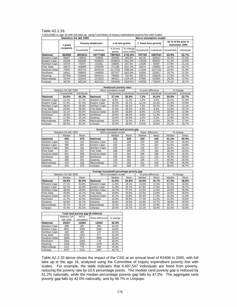
176
Table A2.2.33.
Table A2.2.33 above shows the impact of the CSG at an annual level of R1606 in 2000, with full take up to the age 16, analysed using the Committee of Inquiry expenditure poverty line with scales. For example, the table indicates that 4,497,547 individuals are freed from poverty, reducing the poverty rate by 10.5 percentage points. The median rand poverty gap is reduced by 51.2% nationally, while the median percentage poverty gap falls by 47.3%. The aggregate rand poverty gap falls by 42.0% nationally, and by 46.7% in Limpopo.
CSG(1606) to age 16 with full take-up, using Committee of Inquiry expenditure poverty line with scales
households individuals # of new grants
% change since 2000 households individuals households individuals
National 463699 3815011 19777365 7987821 1722.6% 797740 4497547 20.9% 22.7%Western Cape 59407 139531 703848 260696 438.8% 44745 260537 32.1% 37.0%Eastern Cape 63038 830464 4198320 1836055 2912.6% 176536 956037 21.3% 22.8%Northern Cape 19734 73070 315361 108005 547.3% 13105 66397 17.9% 21.1%Free State 18573 308999 1332936 471188 2537.0% 44074 208804 14.3% 15.7%KwaZulu-Natal 70660 843701 4949219 2117523 2996.8% 173161 1037125 20.5% 21.0%Northwest 34341 289953 1448550 557327 1622.9% 54309 322827 18.7% 22.3%Gauteng 107493 526563 2594514 790000 734.9% 93879 536025 17.8% 20.7%Mpumalanga 43704 220624 1213515 482621 1104.3% 57895 333391 26.2% 27.5%Limpopo 46749 582106 3021102 1364406 2918.6% 140036 776404 24.1% 25.7%
households individuals households individuals households individuals households individualsNational 34.6% 46.3% National 27.4% 35.8% 7.2% 10.5% 20.9% 22.7%Western Cape 13.1% 17.7% Western Cape 8.9% 11.2% 4.2% 6.6% 32.1% 37.0%Eastern Cape 57.5% 67.4% Eastern Cape 45.3% 52.1% 12.2% 15.4% 21.3% 22.8%Northern Cape 39.0% 48.3% Northern Cape 32.0% 38.1% 7.0% 10.2% 17.9% 21.1%Free State 43.9% 55.0% Free State 37.6% 46.3% 6.3% 8.6% 14.3% 15.7%KwaZulu-Natal 41.1% 55.4% KwaZulu-Natal 32.6% 43.8% 8.4% 11.6% 20.5% 21.0%Northwest 36.4% 49.4% Northwest 29.6% 38.4% 6.8% 11.0% 18.7% 22.3%Gauteng 17.0% 25.1% Gauteng 14.0% 20.0% 3.0% 5.2% 17.8% 20.7%Mpumalanga 33.8% 45.9% Mpumalanga 25.0% 33.3% 8.9% 12.6% 26.2% 27.5%Limpopo 56.5% 65.4% Limpopo 42.9% 48.6% 13.6% 16.8% 24.1% 25.7%
Median Mean Median Mean Median Mean Median MeanNational 453 575 National 221 333 232 242 51.2% 42.0%Western Cape 310 410 Western Cape 123 228 270 182 87.1% 44.4%Eastern Cape 496 587 Eastern Cape 226 330 270 257 54.4% 43.8%Northern Cape 365 491 Northern Cape 240 324 126 167 34.4% 34.1%Free State 467 547 Free State 288 365 179 183 38.3% 33.4%KwaZulu-Natal 501 658 KwaZulu-Natal 233 362 268 296 53.6% 45.0%Northwest 468 587 Northwest 256 364 212 223 45.3% 38.0%Gauteng 358 501 Gauteng 214 331 145 171 40.4% 34.0%Mpumalanga 416 533 Mpumalanga 175 293 241 240 57.9% 45.0%Limpopo 476 578 Limpopo 197 308 279 270 58.6% 46.7%
Median Mean Median Mean Median Mean Median MeanNational 39.8% 40.5% National 21.0% 24.8% 18.8% 15.7% 47.3% 38.8%Western Cape 27.1% 30.6% Western Cape 11.5% 18.1% 15.6% 12.5% 57.6% 40.9%Eastern Cape 43.7% 43.4% Eastern Cape 21.8% 25.7% 21.9% 17.6% 50.1% 40.7%Northern Cape 38.0% 39.0% Northern Cape 24.7% 27.2% 13.3% 11.9% 34.9% 30.4%Free State 45.8% 44.7% Free State 29.8% 30.9% 16.0% 13.8% 34.9% 30.8%KwaZulu-Natal 40.5% 41.0% KwaZulu-Natal 20.1% 23.8% 20.4% 17.2% 50.3% 41.9%Northwest 41.7% 42.3% Northwest 24.4% 28.0% 17.3% 14.3% 41.5% 33.9%Gauteng 32.6% 34.7% Gauteng 20.6% 24.0% 12.0% 10.7% 36.9% 30.9%Mpumalanga 34.7% 35.1% Mpumalanga 15.4% 20.1% 19.3% 14.9% 55.7% 42.6%Limpopo 41.4% 42.1% Limpopo 19.4% 23.7% 22.1% 18.4% 53.3% 43.8%
Statistics SA I&E 2000
Micro-simulation Rand difference % change
National 26327 15264 11063 42.0%Western Cape 686 381 305 44.4%Eastern Cape 5851 3290 2560 43.8%Northern Cape 430 284 147 34.1%Free State 2030 1353 677 33.4%KwaZulu-Natal 6669 3671 2999 45.0%Northwest 2042 1266 776 38.0%Gauteng 3168 2090 1078 34.0%Mpumalanga 1411 776 635 45.0%Limpopo 4037 2151 1887 46.7%
Total rand poverty gap (R millions)
Statistics SA I&E 2000 Micro-simulation model
Micro-simulation modelStatistics SA I&E 2000
Poverty Headcount# grant
recipients
% point differenceAverage household percentage poverty gap
Average household rand poverty gap% change
% changeMicro-simulation model
% change
Headcount poverty rates
# of new grants # freed from poverty As % of the poor in September 2000
Statistics SA I&E 2000 % point difference
Statistics SA I&E 2000 Micro-simulation model Rand difference
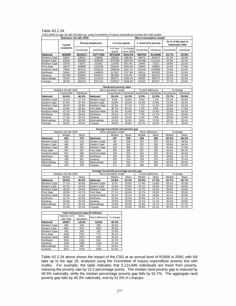
177
Table A2.2.34.
Table A2.2.34 above shows the impact of the CSG at an annual level of R1606 in 2000, with full take up to the age 18, analysed using the Committee of Inquiry expenditure poverty line with scales. For example, the table indicates that 5,114,696 individuals are freed from poverty, reducing the poverty rate by 12.0 percentage points. The median rand poverty gap is reduced by 56.5% nationally, while the median percentage poverty gap falls by 52.7%. The aggregate rand poverty gap falls by 46.3% nationally, and by 51.0% in Limpopo.
CSG(1606) to age 18 with full take-up, using Committee of Inquiry expenditure poverty line with scales
households individuals # of new grants
% change since 2000 households individuals households individuals
National 463699 3815011 19777365 8970206 1934.5% 905704 5114696 23.7% 25.9%Western Cape 59407 139531 703848 290394 488.8% 48473 281673 34.7% 40.0%Eastern Cape 63038 830464 4198320 2070456 3284.5% 201496 1110101 24.3% 26.4%Northern Cape 19734 73070 315361 119795 607.0% 14448 73313 19.8% 23.2%Free State 18573 308999 1332936 542440 2920.6% 50848 238659 16.5% 17.9%KwaZulu-Natal 70660 843701 4949219 2369018 3352.7% 201420 1200882 23.9% 24.3%Northwest 34341 289953 1448550 617407 1797.9% 58114 341933 20.0% 23.6%Gauteng 107493 526563 2594514 882398 820.9% 105289 595125 20.0% 22.9%Mpumalanga 43704 220624 1213515 550271 1259.1% 64095 368773 29.1% 30.4%Limpopo 46749 582106 3021102 1528027 3268.6% 161521 904237 27.7% 29.9%
households individuals households individuals households individuals households individualsNational 34.6% 46.3% National 26.4% 34.3% 8.2% 12.0% 23.7% 25.9%Western Cape 13.1% 17.7% Western Cape 8.5% 10.6% 4.5% 7.1% 34.7% 40.0%Eastern Cape 57.5% 67.4% Eastern Cape 43.6% 49.6% 14.0% 17.8% 24.3% 26.4%Northern Cape 39.0% 48.3% Northern Cape 31.3% 37.1% 7.7% 11.2% 19.8% 23.2%Free State 43.9% 55.0% Free State 36.7% 45.1% 7.2% 9.8% 16.5% 17.9%KwaZulu-Natal 41.1% 55.4% KwaZulu-Natal 31.3% 41.9% 9.8% 13.4% 23.9% 24.3%Northwest 36.4% 49.4% Northwest 29.1% 37.7% 7.3% 11.7% 20.0% 23.6%Gauteng 17.0% 25.1% Gauteng 13.6% 19.4% 3.4% 5.8% 20.0% 22.9%Mpumalanga 33.8% 45.9% Mpumalanga 24.0% 31.9% 9.8% 13.9% 29.1% 30.4%Limpopo 56.5% 65.4% Limpopo 40.8% 45.8% 15.7% 19.6% 27.7% 29.9%
Median Mean Median Mean Median Mean Median MeanNational 453 575 National 197 309 256 266 56.5% 46.3%Western Cape 310 410 Western Cape 98 208 297 202 95.9% 49.3%Eastern Cape 496 587 Eastern Cape 199 304 297 283 59.9% 48.3%Northern Cape 365 491 Northern Cape 218 306 147 185 40.3% 37.6%Free State 467 547 Free State 260 339 207 208 44.4% 38.1%KwaZulu-Natal 501 658 KwaZulu-Natal 199 333 302 325 60.3% 49.3%Northwest 468 587 Northwest 240 342 228 245 48.6% 41.7%Gauteng 358 501 Gauteng 205 314 154 187 42.9% 37.4%Mpumalanga 416 533 Mpumalanga 142 264 274 269 65.9% 50.5%Limpopo 476 578 Limpopo 171 283 306 295 64.2% 51.0%
Median Mean Median Mean Median Mean Median MeanNational 39.8% 40.5% National 18.8% 23.2% 20.9% 17.3% 52.7% 42.7%Western Cape 27.1% 30.6% Western Cape 9.2% 16.8% 17.9% 13.8% 66.1% 45.0%Eastern Cape 43.7% 43.4% Eastern Cape 19.5% 23.9% 24.1% 19.5% 55.3% 44.9%Northern Cape 38.0% 39.0% Northern Cape 23.4% 25.8% 14.7% 13.2% 38.6% 33.8%Free State 45.8% 44.7% Free State 27.1% 28.8% 18.7% 15.9% 40.9% 35.6%KwaZulu-Natal 40.5% 41.0% KwaZulu-Natal 18.2% 22.2% 22.3% 18.8% 55.1% 45.9%Northwest 41.7% 42.3% Northwest 22.4% 26.6% 19.4% 15.7% 46.4% 37.1%Gauteng 32.6% 34.7% Gauteng 19.5% 23.0% 13.1% 11.7% 40.1% 33.6%Mpumalanga 34.7% 35.1% Mpumalanga 13.0% 18.3% 21.6% 16.7% 62.4% 47.7%Limpopo 41.4% 42.1% Limpopo 16.5% 22.0% 24.9% 20.1% 60.2% 47.7%
Statistics SA I&E 2000
Micro-simulation Rand difference % change
National 26327 14134 12192 46.3%Western Cape 686 348 338 49.3%Eastern Cape 5851 3027 2823 48.3%Northern Cape 430 268 162 37.6%Free State 2030 1257 773 38.1%KwaZulu-Natal 6669 3379 3291 49.3%Northwest 2042 1191 851 41.7%Gauteng 3168 1985 1183 37.4%Mpumalanga 1411 699 712 50.5%Limpopo 4037 1978 2059 51.0%
Total rand poverty gap (R millions)
Statistics SA I&E 2000 Micro-simulation model
Micro-simulation modelStatistics SA I&E 2000
Poverty Headcount# grant
recipients
% point differenceAverage household percentage poverty gap
Average household rand poverty gap% change
% changeMicro-simulation model
% change
Headcount poverty rates
# of new grants # freed from poverty As % of the poor in September 2000
Statistics SA I&E 2000 % point difference
Statistics SA I&E 2000 Micro-simulation model Rand difference
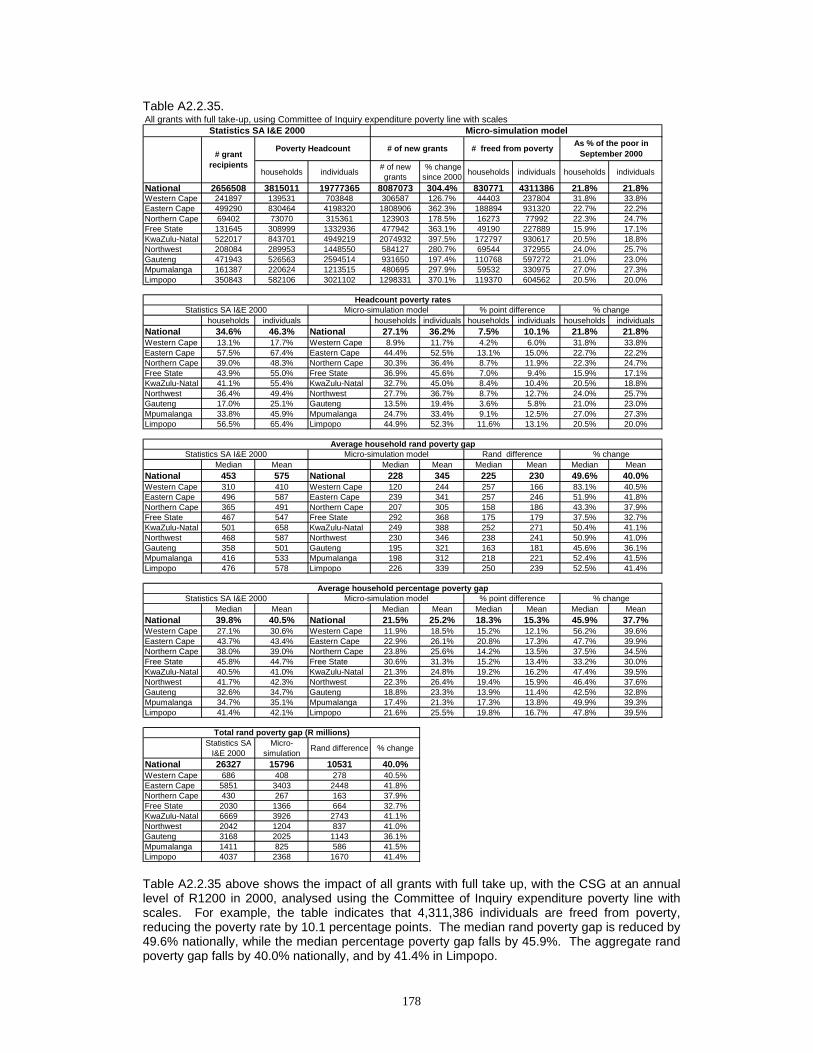
178
Table A2.2.35.
Table A2.2.35 above shows the impact of all grants with full take up, with the CSG at an annual level of R1200 in 2000, analysed using the Committee of Inquiry expenditure poverty line with scales. For example, the table indicates that 4,311,386 individuals are freed from poverty, reducing the poverty rate by 10.1 percentage points. The median rand poverty gap is reduced by 49.6% nationally, while the median percentage poverty gap falls by 45.9%. The aggregate rand poverty gap falls by 40.0% nationally, and by 41.4% in Limpopo.
All grants with full take-up, using Committee of Inquiry expenditure poverty line with scales
households individuals # of new grants
% change since 2000 households individuals households individuals
National 2656508 3815011 19777365 8087073 304.4% 830771 4311386 21.8% 21.8%Western Cape 241897 139531 703848 306587 126.7% 44403 237804 31.8% 33.8%Eastern Cape 499290 830464 4198320 1808906 362.3% 188894 931320 22.7% 22.2%Northern Cape 69402 73070 315361 123903 178.5% 16273 77992 22.3% 24.7%Free State 131645 308999 1332936 477942 363.1% 49190 227889 15.9% 17.1%KwaZulu-Natal 522017 843701 4949219 2074932 397.5% 172797 930617 20.5% 18.8%Northwest 208084 289953 1448550 584127 280.7% 69544 372955 24.0% 25.7%Gauteng 471943 526563 2594514 931650 197.4% 110768 597272 21.0% 23.0%Mpumalanga 161387 220624 1213515 480695 297.9% 59532 330975 27.0% 27.3%Limpopo 350843 582106 3021102 1298331 370.1% 119370 604562 20.5% 20.0%
households individuals households individuals households individuals households individualsNational 34.6% 46.3% National 27.1% 36.2% 7.5% 10.1% 21.8% 21.8%Western Cape 13.1% 17.7% Western Cape 8.9% 11.7% 4.2% 6.0% 31.8% 33.8%Eastern Cape 57.5% 67.4% Eastern Cape 44.4% 52.5% 13.1% 15.0% 22.7% 22.2%Northern Cape 39.0% 48.3% Northern Cape 30.3% 36.4% 8.7% 11.9% 22.3% 24.7%Free State 43.9% 55.0% Free State 36.9% 45.6% 7.0% 9.4% 15.9% 17.1%KwaZulu-Natal 41.1% 55.4% KwaZulu-Natal 32.7% 45.0% 8.4% 10.4% 20.5% 18.8%Northwest 36.4% 49.4% Northwest 27.7% 36.7% 8.7% 12.7% 24.0% 25.7%Gauteng 17.0% 25.1% Gauteng 13.5% 19.4% 3.6% 5.8% 21.0% 23.0%Mpumalanga 33.8% 45.9% Mpumalanga 24.7% 33.4% 9.1% 12.5% 27.0% 27.3%Limpopo 56.5% 65.4% Limpopo 44.9% 52.3% 11.6% 13.1% 20.5% 20.0%
Median Mean Median Mean Median Mean Median MeanNational 453 575 National 228 345 225 230 49.6% 40.0%Western Cape 310 410 Western Cape 120 244 257 166 83.1% 40.5%Eastern Cape 496 587 Eastern Cape 239 341 257 246 51.9% 41.8%Northern Cape 365 491 Northern Cape 207 305 158 186 43.3% 37.9%Free State 467 547 Free State 292 368 175 179 37.5% 32.7%KwaZulu-Natal 501 658 KwaZulu-Natal 249 388 252 271 50.4% 41.1%Northwest 468 587 Northwest 230 346 238 241 50.9% 41.0%Gauteng 358 501 Gauteng 195 321 163 181 45.6% 36.1%Mpumalanga 416 533 Mpumalanga 198 312 218 221 52.4% 41.5%Limpopo 476 578 Limpopo 226 339 250 239 52.5% 41.4%
Median Mean Median Mean Median Mean Median MeanNational 39.8% 40.5% National 21.5% 25.2% 18.3% 15.3% 45.9% 37.7%Western Cape 27.1% 30.6% Western Cape 11.9% 18.5% 15.2% 12.1% 56.2% 39.6%Eastern Cape 43.7% 43.4% Eastern Cape 22.9% 26.1% 20.8% 17.3% 47.7% 39.9%Northern Cape 38.0% 39.0% Northern Cape 23.8% 25.6% 14.2% 13.5% 37.5% 34.5%Free State 45.8% 44.7% Free State 30.6% 31.3% 15.2% 13.4% 33.2% 30.0%KwaZulu-Natal 40.5% 41.0% KwaZulu-Natal 21.3% 24.8% 19.2% 16.2% 47.4% 39.5%Northwest 41.7% 42.3% Northwest 22.3% 26.4% 19.4% 15.9% 46.4% 37.6%Gauteng 32.6% 34.7% Gauteng 18.8% 23.3% 13.9% 11.4% 42.5% 32.8%Mpumalanga 34.7% 35.1% Mpumalanga 17.4% 21.3% 17.3% 13.8% 49.9% 39.3%Limpopo 41.4% 42.1% Limpopo 21.6% 25.5% 19.8% 16.7% 47.8% 39.5%
Statistics SA I&E 2000
Micro-simulation Rand difference % change
National 26327 15796 10531 40.0%Western Cape 686 408 278 40.5%Eastern Cape 5851 3403 2448 41.8%Northern Cape 430 267 163 37.9%Free State 2030 1366 664 32.7%KwaZulu-Natal 6669 3926 2743 41.1%Northwest 2042 1204 837 41.0%Gauteng 3168 2025 1143 36.1%Mpumalanga 1411 825 586 41.5%Limpopo 4037 2368 1670 41.4%
Total rand poverty gap (R millions)
Statistics SA I&E 2000 Micro-simulation model
Micro-simulation modelStatistics SA I&E 2000
Poverty Headcount# grant
recipients
% point differenceAverage household percentage poverty gap
Average household rand poverty gap% change
% changeMicro-simulation model
% change
Headcount poverty rates
# of new grants # freed from poverty As % of the poor in September 2000
Statistics SA I&E 2000 % point difference
Statistics SA I&E 2000 Micro-simulation model Rand difference

179
Table A2.2.36.
Table A2.2.36 above shows the impact of all grants with full take up, with the CSG at an annual level of R1606 in 2000, analysed using the Committee of Inquiry expenditure poverty line with scales. For example, the table indicates that 5,520,683 individuals are freed from poverty, reducing the poverty rate by 12.9 percentage points. The median rand poverty gap is reduced by 59.8% nationally, while the median percentage poverty gap falls by 55.5%. The aggregate rand poverty gap falls by 47.5% nationally, and by 49.9% in Limpopo.
All grants(1606) with full take-up, using Committee of Inquiry expenditure poverty line with scales
households individuals # of new grants
% change since 2000 households individuals households individuals
National 2656508 3815011 19777365 8087073 304.4% 1027393 5520683 26.9% 27.9%Western Cape 241897 139531 703848 306587 126.7% 49899 267156 35.8% 38.0%Eastern Cape 499290 830464 4198320 1808906 362.3% 230597 1180707 27.8% 28.1%Northern Cape 69402 73070 315361 123903 178.5% 19524 94315 26.7% 29.9%Free State 131645 308999 1332936 477942 363.1% 58742 276240 19.0% 20.7%KwaZulu-Natal 522017 843701 4949219 2074932 397.5% 218711 1239640 25.9% 25.0%Northwest 208084 289953 1448550 584127 280.7% 82857 460264 28.6% 31.8%Gauteng 471943 526563 2594514 931650 197.4% 133968 730509 25.4% 28.2%Mpumalanga 161387 220624 1213515 480695 297.9% 69084 388728 31.3% 32.0%Limpopo 350843 582106 3021102 1298331 370.1% 164011 883124 28.2% 29.2%
households individuals households individuals households individuals households individualsNational 34.6% 46.3% National 25.3% 33.4% 9.3% 12.9% 26.9% 27.9%Western Cape 13.1% 17.7% Western Cape 8.4% 11.0% 4.7% 6.7% 35.8% 38.0%Eastern Cape 57.5% 67.4% Eastern Cape 41.5% 48.5% 16.0% 19.0% 27.8% 28.1%Northern Cape 39.0% 48.3% Northern Cape 28.6% 33.9% 10.4% 14.4% 26.7% 29.9%Free State 43.9% 55.0% Free State 35.5% 43.6% 8.3% 11.4% 19.0% 20.7%KwaZulu-Natal 41.1% 55.4% KwaZulu-Natal 30.4% 41.5% 10.6% 13.9% 25.9% 25.0%Northwest 36.4% 49.4% Northwest 26.0% 33.7% 10.4% 15.7% 28.6% 31.8%Gauteng 17.0% 25.1% Gauteng 12.7% 18.1% 4.3% 7.1% 25.4% 28.2%Mpumalanga 33.8% 45.9% Mpumalanga 23.2% 31.2% 10.6% 14.7% 31.3% 32.0%Limpopo 56.5% 65.4% Limpopo 40.6% 46.3% 15.9% 19.1% 28.2% 29.2%
Median Mean Median Mean Median Mean Median MeanNational 453 575 National 182 302 271 273 59.8% 47.5%Western Cape 310 410 Western Cape 85 215 314 194 101.2% 47.5%Eastern Cape 496 587 Eastern Cape 183 295 314 292 63.2% 49.7%Northern Cape 365 491 Northern Cape 178 277 187 214 51.2% 43.6%Free State 467 547 Free State 256 335 211 212 45.2% 38.8%KwaZulu-Natal 501 658 KwaZulu-Natal 193 333 308 325 61.5% 49.4%Northwest 468 587 Northwest 190 309 278 277 59.5% 47.3%Gauteng 358 501 Gauteng 174 292 185 210 51.6% 41.8%Mpumalanga 416 533 Mpumalanga 149 271 266 262 64.1% 49.2%Limpopo 476 578 Limpopo 171 290 305 288 64.0% 49.9%
Median Mean Median Mean Median Mean Median MeanNational 39.8% 40.5% National 17.7% 22.5% 22.1% 18.0% 55.5% 44.4%Western Cape 27.1% 30.6% Western Cape 8.0% 16.5% 19.0% 14.1% 70.3% 46.0%Eastern Cape 43.7% 43.4% Eastern Cape 18.1% 23.0% 25.6% 20.4% 58.5% 47.0%Northern Cape 38.0% 39.0% Northern Cape 20.4% 23.6% 17.6% 15.5% 46.3% 39.6%Free State 45.8% 44.7% Free State 26.8% 28.8% 19.0% 15.9% 41.4% 35.5%KwaZulu-Natal 40.5% 41.0% KwaZulu-Natal 17.0% 21.8% 23.5% 19.2% 58.0% 46.9%Northwest 41.7% 42.3% Northwest 19.3% 24.0% 22.4% 18.3% 53.8% 43.2%Gauteng 32.6% 34.7% Gauteng 16.4% 21.5% 16.2% 13.2% 49.6% 38.0%Mpumalanga 34.7% 35.1% Mpumalanga 13.5% 18.8% 21.1% 16.2% 61.0% 46.3%Limpopo 41.4% 42.1% Limpopo 17.3% 22.2% 24.2% 19.9% 58.3% 47.3%
Statistics SA I&E 2000
Micro-simulation Rand difference % change
National 26327 13829 12497 47.5%Western Cape 686 360 326 47.5%Eastern Cape 5851 2943 2907 49.7%Northern Cape 430 243 188 43.6%Free State 2030 1243 787 38.8%KwaZulu-Natal 6669 3376 3294 49.4%Northwest 2042 1077 965 47.3%Gauteng 3168 1844 1324 41.8%Mpumalanga 1411 717 694 49.2%Limpopo 4037 2024 2013 49.9%
% change
Headcount poverty rates
# of new grants # freed from poverty As % of the poor in September 2000
Statistics SA I&E 2000 % point difference
Statistics SA I&E 2000 Micro-simulation model Rand differenceAverage household rand poverty gap
% change
% changeMicro-simulation model
Total rand poverty gap (R millions)
Statistics SA I&E 2000 Micro-simulation model
Micro-simulation modelStatistics SA I&E 2000
Poverty Headcount# grant
recipients
% point differenceAverage household percentage poverty gap

180
Table A2.2.37.
Table A2.2.37 above shows the impact of the SOAP with 10% increase, analysed using the Committee of Inquiry income poverty line with no scales. For example, the table indicates that 73,053 individuals are freed from poverty, reducing the poverty rate by 0.2 percentage points. The median rand poverty gap is reduced by 1.6% nationally, while the median percentage poverty gap falls by 1.4%. The aggregate rand poverty gap falls by 1.3% nationally, and by 1.2% in Limpopo.
SOAP with 10% increase in take-up, using Committee of Inquiry income poverty line with no scales
households individuals # of new grants
% change since 2000 households individuals households individuals
National 1767591 5040446 25705260 170542 9.6% 23757 73053 0.5% 0.3%Western Cape 115210 270207 1359679 8359 7.3% 396 2376 0.1% 0.2%Eastern Cape 359973 978547 4824104 32942 9.2% 4511 9743 0.5% 0.2%Northern Cape 30040 84444 374307 2600 8.7% 1005 2753 1.2% 0.7%Free State 93003 370687 1574256 8459 9.1% 1363 3478 0.4% 0.2%KwaZulu-Natal 358184 1049229 6063166 32751 9.1% 4949 15116 0.5% 0.2%Northwest 139114 383363 1896409 14017 10.1% 3154 9728 0.8% 0.5%Gauteng 304931 855613 4197757 39316 12.9% 5320 21056 0.6% 0.5%Mpumalanga 97852 330232 1737000 9003 9.2% 1258 3565 0.4% 0.2%Limpopo 269284 718124 3678582 23095 8.6% 1801 5238 0.3% 0.1%
households individuals households individuals households individuals households individualsNational 45.7% 60.2% National 45.5% 60.0% 0.2% 0.2% 0.5% 0.3%Western Cape 25.3% 34.3% Western Cape 25.2% 34.2% 0.0% 0.1% 0.1% 0.2%Eastern Cape 67.8% 77.5% Eastern Cape 67.5% 77.3% 0.3% 0.2% 0.5% 0.2%Northern Cape 45.1% 57.3% Northern Cape 44.6% 56.9% 0.5% 0.4% 1.2% 0.7%Free State 52.6% 64.9% Free State 52.4% 64.8% 0.2% 0.1% 0.4% 0.2%KwaZulu-Natal 51.1% 67.8% KwaZulu-Natal 50.8% 67.6% 0.3% 0.2% 0.5% 0.3%Northwest 48.2% 64.7% Northwest 47.8% 64.4% 0.4% 0.3% 0.8% 0.5%Gauteng 27.7% 40.7% Gauteng 27.5% 40.5% 0.2% 0.2% 0.6% 0.5%Mpumalanga 50.6% 65.7% Mpumalanga 50.4% 65.6% 0.2% 0.1% 0.4% 0.2%Limpopo 69.7% 79.6% Limpopo 69.5% 79.5% 0.2% 0.1% 0.3% 0.1%
Median Mean Median Mean Median Mean Median MeanNational 804 1021 National 791 1008 13 13 1.6% 1.3%Western Cape 515 676 Western Cape 512 673 9 3 1.7% 0.5%Eastern Cape 950 1132 Eastern Cape 942 1116 9 15 0.9% 1.4%Northern Cape 721 896 Northern Cape 721 888 0 8 0.0% 0.9%Free State 783 918 Free State 766 908 17 11 2.1% 1.2%KwaZulu-Natal 966 1252 KwaZulu-Natal 953 1239 13 13 1.4% 1.0%Northwest 762 994 Northwest 759 981 3 13 0.4% 1.3%Gauteng 464 731 Gauteng 448 716 16 15 3.5% 2.1%Mpumalanga 767 966 Mpumalanga 763 958 5 9 0.6% 0.9%Limpopo 962 1116 Limpopo 948 1102 14 14 1.5% 1.2%
Median Mean Median Mean Median Mean Median MeanNational 48.5% 45.4% National 47.9% 44.8% 0.7% 0.6% 1.4% 1.3%Western Cape 30.1% 31.4% Western Cape 30.0% 31.2% 0.1% 0.1% 0.5% 0.4%Eastern Cape 56.7% 52.6% Eastern Cape 56.0% 51.8% 0.7% 0.9% 1.3% 1.7%Northern Cape 47.1% 45.7% Northern Cape 47.1% 45.3% 0.0% 0.4% 0.1% 1.0%Free State 55.0% 50.0% Free State 54.5% 49.5% 0.5% 0.6% 1.0% 1.1%KwaZulu-Natal 52.1% 48.4% KwaZulu-Natal 51.4% 47.9% 0.7% 0.6% 1.4% 1.2%Northwest 47.0% 45.5% Northwest 46.4% 44.8% 0.6% 0.6% 1.3% 1.4%Gauteng 32.2% 33.3% Gauteng 30.5% 32.7% 1.7% 0.6% 5.3% 1.9%Mpumalanga 42.7% 40.9% Mpumalanga 42.1% 40.5% 0.6% 0.4% 1.4% 0.9%Limpopo 54.5% 50.5% Limpopo 53.7% 49.9% 0.8% 0.6% 1.5% 1.1%
Statistics SA I&E 2000
Micro-simulation Rand difference % change
National 61785 61011 774 1.3%Western Cape 2192 2182 11 0.5%Eastern Cape 13290 13110 180 1.4%Northern Cape 908 900 8 0.9%Free State 4084 4037 47 1.2%KwaZulu-Natal 15764 15606 158 1.0%Northwest 4574 4513 61 1.3%Gauteng 7530 7373 157 2.1%Mpumalanga 3829 3795 35 0.9%Limpopo 9613 9496 117 1.2%
Total rand poverty gap (R millions)
Statistics SA I&E 2000 Micro-simulation model
Micro-simulation modelStatistics SA I&E 2000
Poverty Headcount# grant
recipients
% point differenceAverage household percentage poverty gap
Average household rand poverty gap% change
% changeMicro-simulation model
% change
Headcount poverty rates
# of new grants # freed from poverty As % of the poor in September 2000
Statistics SA I&E 2000 % point difference
Statistics SA I&E 2000 Micro-simulation model Rand difference
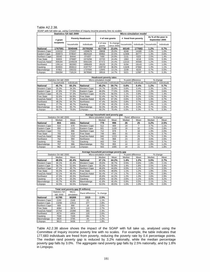
181
Table A2.2.38.
Table A2.2.38 above shows the impact of the SOAP with full take up, analysed using the Committee of Inquiry income poverty line with no scales. For example, the table indicates that 177,683 individuals are freed from poverty, reducing the poverty rate by 0.4 percentage points. The median rand poverty gap is reduced by 3.2% nationally, while the median percentage poverty gap falls by 3.0%. The aggregate rand poverty gap falls by 2.5% nationally, and by 1.8% in Limpopo.
SOAP with full take-up, using Committee of Inquiry income poverty line no scales
households individuals # of new grants
% change since 2000 households individuals households individuals
National 1767591 5040446 25705260 417730 23.6% 60140 177683 1.2% 0.7%Western Cape 115210 270207 1359679 28838 25.0% 6248 14180 2.3% 1.0%Eastern Cape 359973 978547 4824104 80962 22.5% 12306 30777 1.3% 0.6%Northern Cape 30040 84444 374307 7490 24.9% 2131 5325 2.5% 1.4%Free State 93003 370687 1574256 22720 24.4% 1963 4218 0.5% 0.3%KwaZulu-Natal 358184 1049229 6063166 87472 24.4% 12210 35568 1.2% 0.6%Northwest 139114 383363 1896409 28155 20.2% 6194 19143 1.6% 1.0%Gauteng 304931 855613 4197757 109732 36.0% 11628 47660 1.4% 1.1%Mpumalanga 97852 330232 1737000 12845 13.1% 2239 8225 0.7% 0.5%Limpopo 269284 718124 3678582 39516 14.7% 5221 12587 0.7% 0.3%
households individuals households individuals households individuals households individualsNational 45.7% 60.2% National 45.2% 59.7% 0.6% 0.4% 1.2% 0.7%Western Cape 25.3% 34.3% Western Cape 24.7% 33.9% 0.6% 0.4% 2.3% 1.0%Eastern Cape 67.8% 77.5% Eastern Cape 66.9% 77.0% 0.9% 0.5% 1.3% 0.6%Northern Cape 45.1% 57.3% Northern Cape 44.0% 56.5% 1.1% 0.8% 2.5% 1.4%Free State 52.6% 64.9% Free State 52.4% 64.7% 0.3% 0.2% 0.5% 0.3%KwaZulu-Natal 51.1% 67.8% KwaZulu-Natal 50.4% 67.3% 0.6% 0.5% 1.3% 0.7%Northwest 48.2% 64.7% Northwest 47.4% 64.0% 0.8% 0.7% 1.6% 1.0%Gauteng 27.7% 40.7% Gauteng 27.3% 40.2% 0.4% 0.5% 1.4% 1.1%Mpumalanga 50.6% 65.7% Mpumalanga 50.3% 65.4% 0.3% 0.3% 0.7% 0.5%Limpopo 69.7% 79.6% Limpopo 69.2% 79.4% 0.5% 0.3% 0.7% 0.3%
Median Mean Median Mean Median Mean Median MeanNational 804 1021 National 778 996 26 25 3.2% 2.5%Western Cape 515 676 Western Cape 512 669 19 7 3.7% 1.1%Eastern Cape 950 1132 Eastern Cape 931 1100 19 32 2.0% 2.8%Northern Cape 721 896 Northern Cape 712 878 9 18 1.3% 2.0%Free State 783 918 Free State 749 893 33 25 4.2% 2.7%KwaZulu-Natal 966 1252 KwaZulu-Natal 940 1223 26 29 2.7% 2.3%Northwest 762 994 Northwest 740 968 23 26 3.0% 2.6%Gauteng 464 731 Gauteng 443 704 21 27 4.6% 3.7%Mpumalanga 767 966 Mpumalanga 753 955 14 11 1.9% 1.2%Limpopo 962 1116 Limpopo 943 1095 19 21 2.0% 1.8%
Median Mean Median Mean Median Mean Median MeanNational 48.5% 45.4% National 47.1% 44.2% 1.4% 1.2% 3.0% 2.7%Western Cape 30.1% 31.4% Western Cape 29.6% 30.7% 0.5% 0.6% 1.8% 2.1%Eastern Cape 56.7% 52.6% Eastern Cape 55.3% 50.9% 1.4% 1.8% 2.5% 3.4%Northern Cape 47.1% 45.7% Northern Cape 46.6% 44.6% 0.5% 1.1% 1.1% 2.5%Free State 55.0% 50.0% Free State 54.0% 48.8% 1.1% 1.2% 1.9% 2.5%KwaZulu-Natal 52.1% 48.4% KwaZulu-Natal 50.4% 47.1% 1.7% 1.3% 3.3% 2.8%Northwest 47.0% 45.5% Northwest 45.8% 44.2% 1.2% 1.3% 2.6% 2.9%Gauteng 32.2% 33.3% Gauteng 29.6% 32.3% 2.6% 1.1% 8.0% 3.2%Mpumalanga 42.7% 40.9% Mpumalanga 41.8% 40.4% 0.9% 0.5% 2.1% 1.2%Limpopo 54.5% 50.5% Limpopo 53.5% 49.5% 1.0% 1.0% 1.9% 2.0%
Statistics SA I&E 2000
Micro-simulation Rand difference % change
National 61785 60269 1515 2.5%Western Cape 2192 2169 23 1.1%Eastern Cape 13290 12913 377 2.8%Northern Cape 908 890 18 2.0%Free State 4084 3974 110 2.7%KwaZulu-Natal 15764 15399 365 2.3%Northwest 4574 4454 120 2.6%Gauteng 7530 7249 281 3.7%Mpumalanga 3829 3785 44 1.2%Limpopo 9613 9436 177 1.8%
Total rand poverty gap (R millions)
Statistics SA I&E 2000 Micro-simulation model
Micro-simulation modelStatistics SA I&E 2000
Poverty Headcount# grant
recipients
% point differenceAverage household percentage poverty gap
Average household rand poverty gap% change
% changeMicro-simulation model
% change
Headcount poverty rates
# of new grants # freed from poverty As % of the poor in September 2000
Statistics SA I&E 2000 % point difference
Statistics SA I&E 2000 Micro-simulation model Rand difference
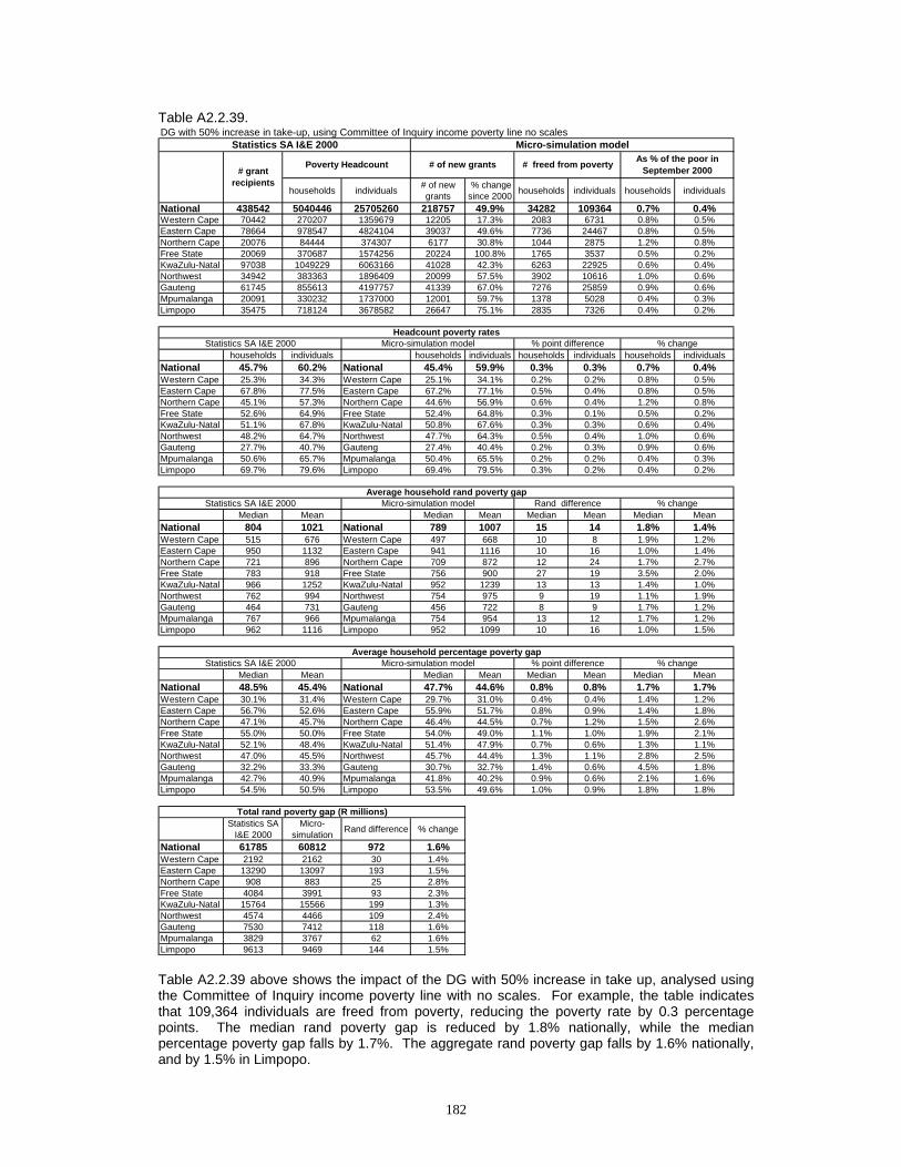
182
Table A2.2.39.
Table A2.2.39 above shows the impact of the DG with 50% increase in take up, analysed using the Committee of Inquiry income poverty line with no scales. For example, the table indicates that 109,364 individuals are freed from poverty, reducing the poverty rate by 0.3 percentage points. The median rand poverty gap is reduced by 1.8% nationally, while the median percentage poverty gap falls by 1.7%. The aggregate rand poverty gap falls by 1.6% nationally, and by 1.5% in Limpopo.
DG with 50% increase in take-up, using Committee of Inquiry income poverty line no scales
households individuals # of new grants
% change since 2000 households individuals households individuals
National 438542 5040446 25705260 218757 49.9% 34282 109364 0.7% 0.4%Western Cape 70442 270207 1359679 12205 17.3% 2083 6731 0.8% 0.5%Eastern Cape 78664 978547 4824104 39037 49.6% 7736 24467 0.8% 0.5%Northern Cape 20076 84444 374307 6177 30.8% 1044 2875 1.2% 0.8%Free State 20069 370687 1574256 20224 100.8% 1765 3537 0.5% 0.2%KwaZulu-Natal 97038 1049229 6063166 41028 42.3% 6263 22925 0.6% 0.4%Northwest 34942 383363 1896409 20099 57.5% 3902 10616 1.0% 0.6%Gauteng 61745 855613 4197757 41339 67.0% 7276 25859 0.9% 0.6%Mpumalanga 20091 330232 1737000 12001 59.7% 1378 5028 0.4% 0.3%Limpopo 35475 718124 3678582 26647 75.1% 2835 7326 0.4% 0.2%
households individuals households individuals households individuals households individualsNational 45.7% 60.2% National 45.4% 59.9% 0.3% 0.3% 0.7% 0.4%Western Cape 25.3% 34.3% Western Cape 25.1% 34.1% 0.2% 0.2% 0.8% 0.5%Eastern Cape 67.8% 77.5% Eastern Cape 67.2% 77.1% 0.5% 0.4% 0.8% 0.5%Northern Cape 45.1% 57.3% Northern Cape 44.6% 56.9% 0.6% 0.4% 1.2% 0.8%Free State 52.6% 64.9% Free State 52.4% 64.8% 0.3% 0.1% 0.5% 0.2%KwaZulu-Natal 51.1% 67.8% KwaZulu-Natal 50.8% 67.6% 0.3% 0.3% 0.6% 0.4%Northwest 48.2% 64.7% Northwest 47.7% 64.3% 0.5% 0.4% 1.0% 0.6%Gauteng 27.7% 40.7% Gauteng 27.4% 40.4% 0.2% 0.3% 0.9% 0.6%Mpumalanga 50.6% 65.7% Mpumalanga 50.4% 65.5% 0.2% 0.2% 0.4% 0.3%Limpopo 69.7% 79.6% Limpopo 69.4% 79.5% 0.3% 0.2% 0.4% 0.2%
Median Mean Median Mean Median Mean Median MeanNational 804 1021 National 789 1007 15 14 1.8% 1.4%Western Cape 515 676 Western Cape 497 668 10 8 1.9% 1.2%Eastern Cape 950 1132 Eastern Cape 941 1116 10 16 1.0% 1.4%Northern Cape 721 896 Northern Cape 709 872 12 24 1.7% 2.7%Free State 783 918 Free State 756 900 27 19 3.5% 2.0%KwaZulu-Natal 966 1252 KwaZulu-Natal 952 1239 13 13 1.4% 1.0%Northwest 762 994 Northwest 754 975 9 19 1.1% 1.9%Gauteng 464 731 Gauteng 456 722 8 9 1.7% 1.2%Mpumalanga 767 966 Mpumalanga 754 954 13 12 1.7% 1.2%Limpopo 962 1116 Limpopo 952 1099 10 16 1.0% 1.5%
Median Mean Median Mean Median Mean Median MeanNational 48.5% 45.4% National 47.7% 44.6% 0.8% 0.8% 1.7% 1.7%Western Cape 30.1% 31.4% Western Cape 29.7% 31.0% 0.4% 0.4% 1.4% 1.2%Eastern Cape 56.7% 52.6% Eastern Cape 55.9% 51.7% 0.8% 0.9% 1.4% 1.8%Northern Cape 47.1% 45.7% Northern Cape 46.4% 44.5% 0.7% 1.2% 1.5% 2.6%Free State 55.0% 50.0% Free State 54.0% 49.0% 1.1% 1.0% 1.9% 2.1%KwaZulu-Natal 52.1% 48.4% KwaZulu-Natal 51.4% 47.9% 0.7% 0.6% 1.3% 1.1%Northwest 47.0% 45.5% Northwest 45.7% 44.4% 1.3% 1.1% 2.8% 2.5%Gauteng 32.2% 33.3% Gauteng 30.7% 32.7% 1.4% 0.6% 4.5% 1.8%Mpumalanga 42.7% 40.9% Mpumalanga 41.8% 40.2% 0.9% 0.6% 2.1% 1.6%Limpopo 54.5% 50.5% Limpopo 53.5% 49.6% 1.0% 0.9% 1.8% 1.8%
Statistics SA I&E 2000
Micro-simulation Rand difference % change
National 61785 60812 972 1.6%Western Cape 2192 2162 30 1.4%Eastern Cape 13290 13097 193 1.5%Northern Cape 908 883 25 2.8%Free State 4084 3991 93 2.3%KwaZulu-Natal 15764 15566 199 1.3%Northwest 4574 4466 109 2.4%Gauteng 7530 7412 118 1.6%Mpumalanga 3829 3767 62 1.6%Limpopo 9613 9469 144 1.5%
% change
Headcount poverty rates
# of new grants # freed from poverty As % of the poor in September 2000
Statistics SA I&E 2000 % point difference
Statistics SA I&E 2000 Micro-simulation model Rand differenceAverage household rand poverty gap
% change
% changeMicro-simulation model
Total rand poverty gap (R millions)
Statistics SA I&E 2000 Micro-simulation model
Micro-simulation modelStatistics SA I&E 2000
Poverty Headcount# grant
recipients
% point differenceAverage household percentage poverty gap

183
Table A2.2.40.
Table A2.2.40 above shows the impact of the DG with full take up, analysed using the Committee of Inquiry income poverty line with no scales. For example, the table indicates that 407,875 individuals are freed from poverty, reducing the poverty rate by 1.0 percentage points. The median rand poverty gap is reduced by 7.6% nationally, while the median percentage poverty gap falls by 6.8%. The aggregate rand poverty gap falls by 5.1% nationally, and by 3.8% in Limpopo.
DG with full take-up, using Committee of Inquiry income poverty line no scales
households individuals # of new grants
% change since 2000 households individuals households individuals
National 438542 5040446 25705260 780318 177.9% 122918 407875 2.4% 1.6%Western Cape 70442 270207 1359679 55546 78.9% 9420 37785 3.5% 2.8%Eastern Cape 78664 978547 4824104 150466 191.3% 27613 73547 2.8% 1.5%Northern Cape 20076 84444 374307 22818 113.7% 3546 10603 4.2% 2.8%Free State 20069 370687 1574256 54619 272.2% 5879 16497 1.6% 1.0%KwaZulu-Natal 97038 1049229 6063166 158093 162.9% 23233 96611 2.2% 1.6%Northwest 34942 383363 1896409 74196 212.3% 13750 39503 3.6% 2.1%Gauteng 61745 855613 4197757 136145 220.5% 21304 78760 2.5% 1.9%Mpumalanga 20091 330232 1737000 52758 262.6% 6567 21127 2.0% 1.2%Limpopo 35475 718124 3678582 75677 213.3% 11606 33442 1.6% 0.9%
households individuals households individuals households individuals households individualsNational 45.7% 60.2% National 44.6% 59.2% 1.1% 1.0% 2.4% 1.6%Western Cape 25.3% 34.3% Western Cape 24.4% 33.3% 0.9% 1.0% 3.5% 2.8%Eastern Cape 67.8% 77.5% Eastern Cape 65.9% 76.3% 1.9% 1.2% 2.8% 1.5%Northern Cape 45.1% 57.3% Northern Cape 43.2% 55.7% 1.9% 1.6% 4.2% 2.8%Free State 52.6% 64.9% Free State 51.8% 64.2% 0.8% 0.7% 1.6% 1.0%KwaZulu-Natal 51.1% 67.8% KwaZulu-Natal 49.9% 66.8% 1.1% 1.1% 2.2% 1.6%Northwest 48.2% 64.7% Northwest 46.5% 63.3% 1.7% 1.3% 3.6% 2.1%Gauteng 27.7% 40.7% Gauteng 27.0% 39.9% 0.7% 0.8% 2.5% 1.9%Mpumalanga 50.6% 65.7% Mpumalanga 49.6% 64.9% 1.0% 0.8% 2.0% 1.2%Limpopo 69.7% 79.6% Limpopo 68.6% 78.9% 1.1% 0.7% 1.6% 0.9%
Median Mean Median Mean Median Mean Median MeanNational 804 1021 National 743 969 61 52 7.6% 5.1%Western Cape 515 676 Western Cape 465 639 57 38 11.1% 5.6%Eastern Cape 950 1132 Eastern Cape 894 1071 57 61 6.0% 5.4%Northern Cape 721 896 Northern Cape 643 814 78 82 10.8% 9.2%Free State 783 918 Free State 732 869 51 49 6.5% 5.3%KwaZulu-Natal 966 1252 KwaZulu-Natal 918 1200 48 53 5.0% 4.2%Northwest 762 994 Northwest 687 918 75 76 9.8% 7.7%Gauteng 464 731 Gauteng 435 694 29 37 6.3% 5.0%Mpumalanga 767 966 Mpumalanga 700 908 67 58 8.7% 6.0%Limpopo 962 1116 Limpopo 919 1073 43 43 4.4% 3.8%
Median Mean Median Mean Median Mean Median MeanNational 48.5% 45.4% National 45.3% 42.8% 3.3% 2.6% 6.8% 5.7%Western Cape 30.1% 31.4% Western Cape 27.2% 29.5% 2.9% 1.9% 9.6% 6.0%Eastern Cape 56.7% 52.6% Eastern Cape 53.4% 49.4% 3.4% 3.3% 5.9% 6.2%Northern Cape 47.1% 45.7% Northern Cape 43.1% 41.5% 4.0% 4.2% 8.5% 9.1%Free State 55.0% 50.0% Free State 52.1% 47.4% 2.9% 2.7% 5.3% 5.3%KwaZulu-Natal 52.1% 48.4% KwaZulu-Natal 49.0% 46.1% 3.1% 2.3% 5.9% 4.8%Northwest 47.0% 45.5% Northwest 42.4% 41.6% 4.7% 3.9% 9.9% 8.6%Gauteng 32.2% 33.3% Gauteng 29.2% 31.5% 2.9% 1.8% 9.2% 5.5%Mpumalanga 42.7% 40.9% Mpumalanga 39.1% 38.3% 3.6% 2.6% 8.3% 6.3%Limpopo 54.5% 50.5% Limpopo 51.5% 48.2% 3.0% 2.3% 5.5% 4.6%
Statistics SA I&E 2000
Micro-simulation Rand difference % change
National 61785 58658 3126 5.1%Western Cape 2192 2071 122 5.6%Eastern Cape 13290 12572 718 5.4%Northern Cape 908 825 83 9.2%Free State 4084 3868 217 5.3%KwaZulu-Natal 15764 15103 661 4.2%Northwest 4574 4222 352 7.7%Gauteng 7530 7153 377 5.0%Mpumalanga 3829 3600 229 6.0%Limpopo 9613 9246 367 3.8%
% change
Headcount poverty rates
# of new grants # freed from poverty As % of the poor in September 2000
Statistics SA I&E 2000 % point difference
Statistics SA I&E 2000 Micro-simulation model Rand differenceAverage household rand poverty gap
% change
% changeMicro-simulation model
Total rand poverty gap (R millions)
Statistics SA I&E 2000 Micro-simulation model
Micro-simulation modelStatistics SA I&E 2000
Poverty Headcount# grant
recipients
% point differenceAverage household percentage poverty gap

184
Table A2.2.41.
Table A2.2.41 above shows the impact of the CSG at an annual level of R1200 in 2000, with full take up to the age 7, analysed using the Committee of Inquiry income poverty line with no scales. For example, the table indicates that 355,178 individuals are freed from poverty, reducing the poverty rate by 0.8 percentage points. The median rand poverty gap is reduced by 8.7% nationally, while the median percentage poverty gap falls by 7.2%. The aggregate rand poverty gap falls by 7.4% nationally, and by 7.7% in Limpopo.
CSG to age 7 with full take-up, using Committee of Inquiry income poverty line with no scales
households individuals # of new grants
% change since 2000 households individuals households individuals
National 463699 5040446 25705260 4030489 869.2% 72967 355178 1.4% 1.4%Western Cape 59407 270207 1359679 217766 366.6% 10571 51008 3.9% 3.8%Eastern Cape 63038 978547 4824104 772770 1225.9% 9883 45184 1.0% 0.9%Northern Cape 19734 84444 374307 57803 292.9% 1710 6723 2.0% 1.8%Free State 18573 370687 1574256 205158 1104.6% 2880 11192 0.8% 0.7%KwaZulu-Natal 70660 1049229 6063166 1034041 1463.4% 8094 42204 0.8% 0.7%Northwest 34341 383363 1896409 276520 805.2% 4988 24670 1.3% 1.3%Gauteng 107493 855613 4197757 571770 531.9% 20468 103349 2.4% 2.5%Mpumalanga 43704 330232 1737000 256873 587.8% 4781 23756 1.4% 1.4%Limpopo 46749 718124 3678582 637788 1364.3% 9592 47092 1.3% 1.3%
households individuals households individuals households individuals households individualsNational 45.7% 60.2% National 45.0% 59.3% 0.7% 0.8% 1.4% 1.4%Western Cape 25.3% 34.3% Western Cape 24.3% 33.0% 1.0% 1.3% 3.9% 3.8%Eastern Cape 67.8% 77.5% Eastern Cape 67.1% 76.8% 0.7% 0.7% 1.0% 0.9%Northern Cape 45.1% 57.3% Northern Cape 44.2% 56.3% 0.9% 1.0% 2.0% 1.8%Free State 52.6% 64.9% Free State 52.2% 64.4% 0.4% 0.5% 0.8% 0.7%KwaZulu-Natal 51.1% 67.8% KwaZulu-Natal 50.7% 67.4% 0.4% 0.5% 0.8% 0.7%Northwest 48.2% 64.7% Northwest 47.6% 63.8% 0.6% 0.8% 1.3% 1.3%Gauteng 27.7% 40.7% Gauteng 27.0% 39.7% 0.7% 1.0% 2.4% 2.5%Mpumalanga 50.6% 65.7% Mpumalanga 49.9% 64.8% 0.7% 0.9% 1.4% 1.4%Limpopo 69.7% 79.6% Limpopo 68.8% 78.6% 0.9% 1.0% 1.3% 1.3%
Median Mean Median Mean Median Mean Median MeanNational 804 1021 National 734 946 70 75 8.7% 7.4%Western Cape 515 676 Western Cape 438 608 69 68 13.4% 10.1%Eastern Cape 950 1132 Eastern Cape 881 1055 69 77 7.3% 6.8%Northern Cape 721 896 Northern Cape 652 831 69 65 9.5% 7.3%Free State 783 918 Free State 735 865 48 53 6.1% 5.8%KwaZulu-Natal 966 1252 KwaZulu-Natal 899 1157 67 95 6.9% 7.6%Northwest 762 994 Northwest 695 927 67 67 8.8% 6.8%Gauteng 464 731 Gauteng 398 674 66 57 14.3% 7.8%Mpumalanga 767 966 Mpumalanga 685 893 82 74 10.7% 7.6%Limpopo 962 1116 Limpopo 894 1030 68 86 7.1% 7.7%
Median Mean Median Mean Median Mean Median MeanNational 48.5% 45.4% National 45.1% 42.3% 3.5% 3.2% 7.2% 6.9%Western Cape 30.1% 31.4% Western Cape 26.4% 28.2% 3.8% 3.2% 12.5% 10.1%Eastern Cape 56.7% 52.6% Eastern Cape 53.5% 49.4% 3.3% 3.3% 5.8% 6.2%Northern Cape 47.1% 45.7% Northern Cape 43.8% 42.6% 3.3% 3.1% 6.9% 6.8%Free State 55.0% 50.0% Free State 51.6% 47.4% 3.5% 2.7% 6.3% 5.3%KwaZulu-Natal 52.1% 48.4% KwaZulu-Natal 48.2% 44.9% 3.9% 3.5% 7.5% 7.3%Northwest 47.0% 45.5% Northwest 43.6% 42.7% 3.4% 2.8% 7.2% 6.1%Gauteng 32.2% 33.3% Gauteng 28.6% 30.8% 3.5% 2.6% 11.0% 7.7%Mpumalanga 42.7% 40.9% Mpumalanga 39.8% 37.8% 2.9% 3.1% 6.8% 7.5%Limpopo 54.5% 50.5% Limpopo 50.9% 46.9% 3.6% 3.6% 6.6% 7.1%
Statistics SA I&E 2000
Micro-simulation Rand difference % change
National 61785 57234 4551 7.4%Western Cape 2192 1972 221 10.1%Eastern Cape 13290 12385 905 6.8%Northern Cape 908 842 66 7.3%Free State 4084 3849 235 5.8%KwaZulu-Natal 15764 14569 1196 7.6%Northwest 4574 4265 309 6.8%Gauteng 7530 6940 589 7.8%Mpumalanga 3829 3537 292 7.6%Limpopo 9613 8874 739 7.7%
% change
Headcount poverty rates
# of new grants # freed from poverty As % of the poor in September 2000
Statistics SA I&E 2000 % point difference
Statistics SA I&E 2000 Micro-simulation model Rand differenceAverage household rand poverty gap
% change
% changeMicro-simulation model
Total rand poverty gap (R millions)
Statistics SA I&E 2000 Micro-simulation model
Micro-simulation modelStatistics SA I&E 2000
Poverty Headcount# grant
recipients
% point differenceAverage household percentage poverty gap

185
Table A2.2.42.
Table A2.2.42 above shows the impact of the CSG at an annual level of R1200 in 2000, with full take up to the age 9, analysed using the Committee of Inquiry income poverty line with no scales. For example, the table indicates that 466,537 individuals are freed from poverty, reducing the poverty rate by 1.1 percentage points. The median rand poverty gap is reduced by 11.5% nationally, while the median percentage poverty gap falls by 9.9%. The aggregate rand poverty gap falls by 9.9% nationally, and by 10.3% in Limpopo.
CSG to age 9 with full take-up, using Committee of Inquiry income poverty line with no scales
households individuals # of new grants
% change since 2000 households individuals households individuals
National 463699 5040446 25705260 5421401 1169.2% 95730 466537 1.9% 1.8%Western Cape 59407 270207 1359679 281355 473.6% 14121 68052 5.2% 5.0%Eastern Cape 63038 978547 4824104 1050741 1666.8% 13130 57303 1.3% 1.2%Northern Cape 19734 84444 374307 74167 375.8% 2215 9356 2.6% 2.5%Free State 18573 370687 1574256 280132 1508.3% 3522 15058 1.0% 1.0%KwaZulu-Natal 70660 1049229 6063166 1393059 1971.5% 12494 66536 1.2% 1.1%Northwest 34341 383363 1896409 376003 1094.9% 5854 29520 1.5% 1.6%Gauteng 107493 855613 4197757 756301 703.6% 26368 132789 3.1% 3.2%Mpumalanga 43704 330232 1737000 355227 812.8% 6145 30996 1.9% 1.8%Limpopo 46749 718124 3678582 854416 1827.7% 11881 56927 1.7% 1.5%
households individuals households individuals households individuals households individualsNational 45.7% 60.2% National 44.8% 59.1% 0.9% 1.1% 1.9% 1.8%Western Cape 25.3% 34.3% Western Cape 24.0% 32.6% 1.3% 1.7% 5.2% 5.0%Eastern Cape 67.8% 77.5% Eastern Cape 66.9% 76.6% 0.9% 0.9% 1.3% 1.2%Northern Cape 45.1% 57.3% Northern Cape 43.9% 55.9% 1.2% 1.4% 2.6% 2.5%Free State 52.6% 64.9% Free State 52.1% 64.3% 0.5% 0.6% 1.0% 1.0%KwaZulu-Natal 51.1% 67.8% KwaZulu-Natal 50.5% 67.1% 0.6% 0.7% 1.2% 1.1%Northwest 48.2% 64.7% Northwest 47.5% 63.7% 0.7% 1.0% 1.5% 1.6%Gauteng 27.7% 40.7% Gauteng 26.8% 39.4% 0.9% 1.3% 3.1% 3.2%Mpumalanga 50.6% 65.7% Mpumalanga 49.7% 64.5% 0.9% 1.2% 1.9% 1.8%Limpopo 69.7% 79.6% Limpopo 68.5% 78.4% 1.2% 1.2% 1.7% 1.5%
Median Mean Median Mean Median Mean Median MeanNational 804 1021 National 711 920 93 101 11.5% 9.9%Western Cape 515 676 Western Cape 431 588 86 88 16.7% 13.1%Eastern Cape 950 1132 Eastern Cape 865 1027 86 105 9.0% 9.3%Northern Cape 721 896 Northern Cape 623 813 98 83 13.6% 9.3%Free State 783 918 Free State 726 846 57 73 7.3% 7.9%KwaZulu-Natal 966 1252 KwaZulu-Natal 881 1124 85 128 8.8% 10.2%Northwest 762 994 Northwest 675 903 87 91 11.4% 9.2%Gauteng 464 731 Gauteng 386 655 78 75 16.7% 10.3%Mpumalanga 767 966 Mpumalanga 658 865 110 101 14.3% 10.5%Limpopo 962 1116 Limpopo 865 1001 97 115 10.0% 10.3%
Median Mean Median Mean Median Mean Median MeanNational 48.5% 45.4% National 43.8% 41.2% 4.8% 4.2% 9.9% 9.4%Western Cape 30.1% 31.4% Western Cape 25.2% 27.3% 4.9% 4.0% 16.3% 12.9%Eastern Cape 56.7% 52.6% Eastern Cape 51.8% 48.2% 4.9% 4.5% 8.7% 8.5%Northern Cape 47.1% 45.7% Northern Cape 43.2% 41.7% 3.9% 4.0% 8.2% 8.7%Free State 55.0% 50.0% Free State 50.3% 46.3% 4.7% 3.7% 8.5% 7.4%KwaZulu-Natal 52.1% 48.4% KwaZulu-Natal 47.0% 43.6% 5.1% 4.8% 9.9% 9.9%Northwest 47.0% 45.5% Northwest 42.7% 41.7% 4.3% 3.8% 9.2% 8.3%Gauteng 32.2% 33.3% Gauteng 27.7% 30.0% 4.5% 3.4% 13.9% 10.1%Mpumalanga 42.7% 40.9% Mpumalanga 38.0% 36.7% 4.6% 4.2% 10.9% 10.3%Limpopo 54.5% 50.5% Limpopo 49.6% 45.6% 4.9% 4.9% 9.0% 9.6%
Statistics SA I&E 2000
Micro-simulation Rand difference % change
National 61785 55664 6121 9.9%Western Cape 2192 1906 286 13.1%Eastern Cape 13290 12060 1230 9.3%Northern Cape 908 824 84 9.3%Free State 4084 3761 323 7.9%KwaZulu-Natal 15764 14150 1614 10.2%Northwest 4574 4156 419 9.2%Gauteng 7530 6755 775 10.3%Mpumalanga 3829 3427 402 10.5%Limpopo 9613 8626 987 10.3%
% change
Headcount poverty rates
# of new grants # freed from poverty As % of the poor in September 2000
Statistics SA I&E 2000 % point difference
Statistics SA I&E 2000 Micro-simulation model Rand differenceAverage household rand poverty gap
% change
% changeMicro-simulation model
Total rand poverty gap (R millions)
Statistics SA I&E 2000 Micro-simulation model
Micro-simulation modelStatistics SA I&E 2000
Poverty Headcount# grant
recipients
% point differenceAverage household percentage poverty gap

186
Table A2.2.43.
Table A2.2.43 above shows the impact of the CSG at an annual level of R1200 in 2000, with full take up to the age 11, analysed using the Committee of Inquiry income poverty line with no scales. For example, the table indicates that 597,970 individuals are freed from poverty, reducing the poverty rate by 1.4 percentage points. The median rand poverty gap is reduced by 15.0% nationally, while the median percentage poverty gap falls by 12.7%. The aggregate rand poverty gap falls by 12.6% nationally, and by 13.1% in Limpopo.
CSG to age 11 with full take-up, using Committee of Inquiry income poverty line with no scales
households individuals # of new grants
% change since 2000 households individuals households individuals
National 463699 5040446 25705260 6894195 1486.8% 120090 597970 2.4% 2.3%Western Cape 59407 270207 1359679 357630 602.0% 18140 90642 6.7% 6.7%Eastern Cape 63038 978547 4824104 1357441 2153.4% 15102 68844 1.5% 1.4%Northern Cape 19734 84444 374307 91827 465.3% 2436 10262 2.9% 2.7%Free State 18573 370687 1574256 359829 1937.4% 3831 15676 1.0% 1.0%KwaZulu-Natal 70660 1049229 6063166 1747696 2473.4% 17956 96235 1.7% 1.6%Northwest 34341 383363 1896409 485992 1415.2% 7810 38609 2.0% 2.0%Gauteng 107493 855613 4197757 942266 876.6% 34083 176942 4.0% 4.2%Mpumalanga 43704 330232 1737000 456824 1045.3% 7052 34371 2.1% 2.0%Limpopo 46749 718124 3678582 1094690 2341.6% 13680 66389 1.9% 1.8%
households individuals households individuals households individuals households individualsNational 45.7% 60.2% National 44.6% 58.8% 1.1% 1.4% 2.4% 2.3%Western Cape 25.3% 34.3% Western Cape 23.6% 32.0% 1.7% 2.3% 6.7% 6.7%Eastern Cape 67.8% 77.5% Eastern Cape 66.7% 76.4% 1.0% 1.1% 1.5% 1.4%Northern Cape 45.1% 57.3% Northern Cape 43.8% 55.8% 1.3% 1.6% 2.9% 2.7%Free State 52.6% 64.9% Free State 52.1% 64.3% 0.5% 0.6% 1.0% 1.0%KwaZulu-Natal 51.1% 67.8% KwaZulu-Natal 50.2% 66.8% 0.9% 1.1% 1.7% 1.6%Northwest 48.2% 64.7% Northwest 47.2% 63.4% 1.0% 1.3% 2.0% 2.0%Gauteng 27.7% 40.7% Gauteng 26.6% 39.0% 1.1% 1.7% 4.0% 4.2%Mpumalanga 50.6% 65.7% Mpumalanga 49.6% 64.4% 1.1% 1.3% 2.1% 2.0%Limpopo 69.7% 79.6% Limpopo 68.4% 78.2% 1.3% 1.4% 1.9% 1.8%
Median Mean Median Mean Median Mean Median MeanNational 804 1021 National 683 893 121 128 15.0% 12.6%Western Cape 515 676 Western Cape 403 564 117 113 22.8% 16.6%Eastern Cape 950 1132 Eastern Cape 833 997 117 135 12.3% 12.0%Northern Cape 721 896 Northern Cape 611 793 110 103 15.3% 11.5%Free State 783 918 Free State 693 825 89 93 11.4% 10.2%KwaZulu-Natal 966 1252 KwaZulu-Natal 851 1092 114 160 11.8% 12.8%Northwest 762 994 Northwest 650 877 112 118 14.7% 11.8%Gauteng 464 731 Gauteng 367 637 97 94 20.9% 12.8%Mpumalanga 767 966 Mpumalanga 642 837 126 129 16.4% 13.4%Limpopo 962 1116 Limpopo 832 969 130 146 13.5% 13.1%
Median Mean Median Mean Median Mean Median MeanNational 48.5% 45.4% National 42.4% 40.0% 6.2% 5.4% 12.7% 11.8%Western Cape 30.1% 31.4% Western Cape 23.3% 26.2% 6.8% 5.1% 22.5% 16.4%Eastern Cape 56.7% 52.6% Eastern Cape 50.6% 46.9% 6.1% 5.8% 10.8% 11.0%Northern Cape 47.1% 45.7% Northern Cape 42.1% 40.8% 5.0% 4.8% 10.5% 10.6%Free State 55.0% 50.0% Free State 49.4% 45.4% 5.6% 4.7% 10.2% 9.3%KwaZulu-Natal 52.1% 48.4% KwaZulu-Natal 45.3% 42.5% 6.9% 6.0% 13.2% 12.3%Northwest 47.0% 45.5% Northwest 40.9% 40.6% 6.1% 4.9% 13.0% 10.8%Gauteng 32.2% 33.3% Gauteng 27.1% 29.2% 5.1% 4.1% 15.7% 12.3%Mpumalanga 42.7% 40.9% Mpumalanga 36.0% 35.5% 6.7% 5.4% 15.7% 13.1%Limpopo 54.5% 50.5% Limpopo 48.3% 44.2% 6.2% 6.2% 11.4% 12.4%
Statistics SA I&E 2000
Micro-simulation Rand difference % change
National 61785 54022 7763 12.6%Western Cape 2192 1827 365 16.6%Eastern Cape 13290 11702 1588 12.0%Northern Cape 908 803 105 11.5%Free State 4084 3670 415 10.2%KwaZulu-Natal 15764 13751 2014 12.8%Northwest 4574 4032 542 11.8%Gauteng 7530 6567 963 12.8%Mpumalanga 3829 3317 512 13.4%Limpopo 9613 8353 1260 13.1%
% change
Headcount poverty rates
# of new grants # freed from poverty As % of the poor in September 2000
Statistics SA I&E 2000 % point difference
Statistics SA I&E 2000 Micro-simulation model Rand differenceAverage household rand poverty gap
% change
% changeMicro-simulation model
Total rand poverty gap (R millions)
Statistics SA I&E 2000 Micro-simulation model
Micro-simulation modelStatistics SA I&E 2000
Poverty Headcount# grant
recipients
% point differenceAverage household percentage poverty gap
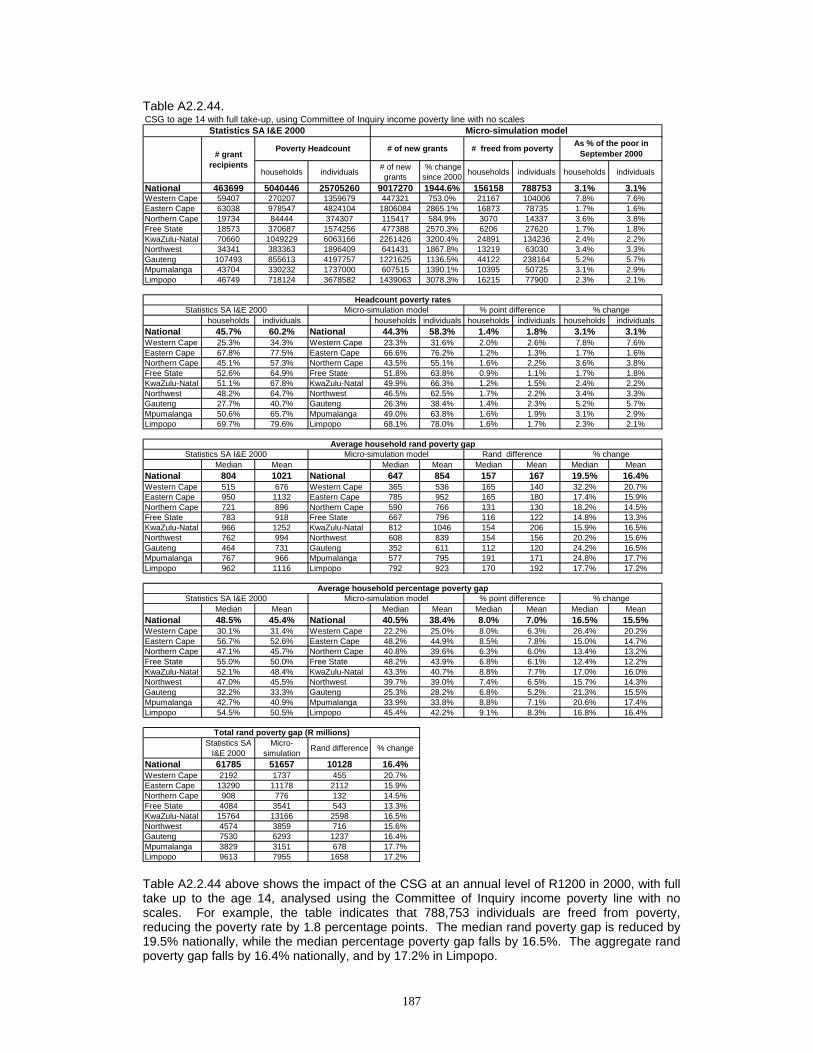
187
Table A2.2.44.
Table A2.2.44 above shows the impact of the CSG at an annual level of R1200 in 2000, with full take up to the age 14, analysed using the Committee of Inquiry income poverty line with no scales. For example, the table indicates that 788,753 individuals are freed from poverty, reducing the poverty rate by 1.8 percentage points. The median rand poverty gap is reduced by 19.5% nationally, while the median percentage poverty gap falls by 16.5%. The aggregate rand poverty gap falls by 16.4% nationally, and by 17.2% in Limpopo.
CSG to age 14 with full take-up, using Committee of Inquiry income poverty line with no scales
households individuals # of new grants
% change since 2000 households individuals households individuals
National 463699 5040446 25705260 9017270 1944.6% 156158 788753 3.1% 3.1%Western Cape 59407 270207 1359679 447321 753.0% 21167 104006 7.8% 7.6%Eastern Cape 63038 978547 4824104 1806084 2865.1% 16873 78735 1.7% 1.6%Northern Cape 19734 84444 374307 115417 584.9% 3070 14337 3.6% 3.8%Free State 18573 370687 1574256 477388 2570.3% 6206 27620 1.7% 1.8%KwaZulu-Natal 70660 1049229 6063166 2261426 3200.4% 24891 134236 2.4% 2.2%Northwest 34341 383363 1896409 641431 1867.8% 13219 63030 3.4% 3.3%Gauteng 107493 855613 4197757 1221625 1136.5% 44122 238164 5.2% 5.7%Mpumalanga 43704 330232 1737000 607515 1390.1% 10395 50725 3.1% 2.9%Limpopo 46749 718124 3678582 1439063 3078.3% 16215 77900 2.3% 2.1%
households individuals households individuals households individuals households individualsNational 45.7% 60.2% National 44.3% 58.3% 1.4% 1.8% 3.1% 3.1%Western Cape 25.3% 34.3% Western Cape 23.3% 31.6% 2.0% 2.6% 7.8% 7.6%Eastern Cape 67.8% 77.5% Eastern Cape 66.6% 76.2% 1.2% 1.3% 1.7% 1.6%Northern Cape 45.1% 57.3% Northern Cape 43.5% 55.1% 1.6% 2.2% 3.6% 3.8%Free State 52.6% 64.9% Free State 51.8% 63.8% 0.9% 1.1% 1.7% 1.8%KwaZulu-Natal 51.1% 67.8% KwaZulu-Natal 49.9% 66.3% 1.2% 1.5% 2.4% 2.2%Northwest 48.2% 64.7% Northwest 46.5% 62.5% 1.7% 2.2% 3.4% 3.3%Gauteng 27.7% 40.7% Gauteng 26.3% 38.4% 1.4% 2.3% 5.2% 5.7%Mpumalanga 50.6% 65.7% Mpumalanga 49.0% 63.8% 1.6% 1.9% 3.1% 2.9%Limpopo 69.7% 79.6% Limpopo 68.1% 78.0% 1.6% 1.7% 2.3% 2.1%
Median Mean Median Mean Median Mean Median MeanNational 804 1021 National 647 854 157 167 19.5% 16.4%Western Cape 515 676 Western Cape 365 536 165 140 32.2% 20.7%Eastern Cape 950 1132 Eastern Cape 785 952 165 180 17.4% 15.9%Northern Cape 721 896 Northern Cape 590 766 131 130 18.2% 14.5%Free State 783 918 Free State 667 796 116 122 14.8% 13.3%KwaZulu-Natal 966 1252 KwaZulu-Natal 812 1046 154 206 15.9% 16.5%Northwest 762 994 Northwest 608 839 154 156 20.2% 15.6%Gauteng 464 731 Gauteng 352 611 112 120 24.2% 16.5%Mpumalanga 767 966 Mpumalanga 577 795 191 171 24.8% 17.7%Limpopo 962 1116 Limpopo 792 923 170 192 17.7% 17.2%
Median Mean Median Mean Median Mean Median MeanNational 48.5% 45.4% National 40.5% 38.4% 8.0% 7.0% 16.5% 15.5%Western Cape 30.1% 31.4% Western Cape 22.2% 25.0% 8.0% 6.3% 26.4% 20.2%Eastern Cape 56.7% 52.6% Eastern Cape 48.2% 44.9% 8.5% 7.8% 15.0% 14.7%Northern Cape 47.1% 45.7% Northern Cape 40.8% 39.6% 6.3% 6.0% 13.4% 13.2%Free State 55.0% 50.0% Free State 48.2% 43.9% 6.8% 6.1% 12.4% 12.2%KwaZulu-Natal 52.1% 48.4% KwaZulu-Natal 43.3% 40.7% 8.8% 7.7% 17.0% 16.0%Northwest 47.0% 45.5% Northwest 39.7% 39.0% 7.4% 6.5% 15.7% 14.3%Gauteng 32.2% 33.3% Gauteng 25.3% 28.2% 6.8% 5.2% 21.3% 15.5%Mpumalanga 42.7% 40.9% Mpumalanga 33.9% 33.8% 8.8% 7.1% 20.6% 17.4%Limpopo 54.5% 50.5% Limpopo 45.4% 42.2% 9.1% 8.3% 16.8% 16.4%
Statistics SA I&E 2000
Micro-simulation Rand difference % change
National 61785 51657 10128 16.4%Western Cape 2192 1737 455 20.7%Eastern Cape 13290 11178 2112 15.9%Northern Cape 908 776 132 14.5%Free State 4084 3541 543 13.3%KwaZulu-Natal 15764 13166 2598 16.5%Northwest 4574 3859 716 15.6%Gauteng 7530 6293 1237 16.4%Mpumalanga 3829 3151 678 17.7%Limpopo 9613 7955 1658 17.2%
% change
Headcount poverty rates
# of new grants # freed from poverty As % of the poor in September 2000
Statistics SA I&E 2000 % point difference
Statistics SA I&E 2000 Micro-simulation model Rand differenceAverage household rand poverty gap
% change
% changeMicro-simulation model
Total rand poverty gap (R millions)
Statistics SA I&E 2000 Micro-simulation model
Micro-simulation modelStatistics SA I&E 2000
Poverty Headcount# grant
recipients
% point differenceAverage household percentage poverty gap

188
Table A2.2.45.
Table A2.2.45 above shows the impact of the CSG at an annual level of R1200 in 2000, with full take up to the age 16, analysed using the Committee of Inquiry income poverty line with no scales. For example, the table indicates that 931,992 individuals are freed from poverty, reducing the poverty rate by 2.2 percentage points. The median rand poverty gap is reduced by 23.0% nationally, while the median percentage poverty gap falls by 19.1%. The aggregate rand poverty gap falls by 18.9% nationally, and by 20.0% in Limpopo.
CSG to age 16 with full take-up, using Committee of Inquiry income poverty line with no scales
households individuals # of new grants
% change since 2000 households individuals households individuals
National 463699 5040446 25705260 10425391 2248.3% 187864 931992 3.7% 3.6%Western Cape 59407 270207 1359679 517005 870.3% 23552 116043 8.7% 8.5%Eastern Cape 63038 978547 4824104 2103551 3337.0% 21345 96585 2.2% 2.0%Northern Cape 19734 84444 374307 132813 673.0% 3415 16029 4.0% 4.3%Free State 18573 370687 1574256 560084 3015.6% 8798 38937 2.4% 2.5%KwaZulu-Natal 70660 1049229 6063166 2611909 3696.4% 32825 177906 3.1% 2.9%Northwest 34341 383363 1896409 743994 2166.5% 15030 69207 3.9% 3.6%Gauteng 107493 855613 4197757 1375524 1279.6% 50754 271035 5.9% 6.5%Mpumalanga 43704 330232 1737000 706884 1617.4% 12571 59038 3.8% 3.4%Limpopo 46749 718124 3678582 1673627 3580.0% 19574 87212 2.7% 2.4%
households individuals households individuals households individuals households individualsNational 45.7% 60.2% National 44.0% 58.0% 1.7% 2.2% 3.7% 3.6%Western Cape 25.3% 34.3% Western Cape 23.1% 31.3% 2.2% 2.9% 8.7% 8.5%Eastern Cape 67.8% 77.5% Eastern Cape 66.3% 75.9% 1.5% 1.6% 2.2% 2.0%Northern Cape 45.1% 57.3% Northern Cape 43.3% 54.9% 1.8% 2.5% 4.0% 4.3%Free State 52.6% 64.9% Free State 51.4% 63.3% 1.2% 1.6% 2.4% 2.5%KwaZulu-Natal 51.1% 67.8% KwaZulu-Natal 49.5% 65.8% 1.6% 2.0% 3.1% 2.9%Northwest 48.2% 64.7% Northwest 46.3% 62.3% 1.9% 2.4% 3.9% 3.6%Gauteng 27.7% 40.7% Gauteng 26.0% 38.1% 1.6% 2.6% 5.9% 6.5%Mpumalanga 50.6% 65.7% Mpumalanga 48.7% 63.5% 1.9% 2.2% 3.8% 3.4%Limpopo 69.7% 79.6% Limpopo 67.8% 77.7% 1.9% 1.9% 2.7% 2.4%
Median Mean Median Mean Median Mean Median MeanNational 804 1021 National 619 828 185 193 23.0% 18.9%Western Cape 515 676 Western Cape 353 514 198 162 38.6% 23.9%Eastern Cape 950 1132 Eastern Cape 752 923 198 209 20.9% 18.4%Northern Cape 721 896 Northern Cape 564 747 157 149 21.8% 16.6%Free State 783 918 Free State 648 775 134 143 17.2% 15.6%KwaZulu-Natal 966 1252 KwaZulu-Natal 785 1014 181 238 18.7% 19.0%Northwest 762 994 Northwest 595 814 167 180 21.9% 18.1%Gauteng 464 731 Gauteng 337 596 127 135 27.4% 18.5%Mpumalanga 767 966 Mpumalanga 545 768 222 198 29.0% 20.5%Limpopo 962 1116 Limpopo 751 893 211 223 21.9% 20.0%
Median Mean Median Mean Median Mean Median MeanNational 48.5% 45.4% National 39.3% 37.3% 9.3% 8.1% 19.1% 17.9%Western Cape 30.1% 31.4% Western Cape 20.8% 24.1% 9.3% 7.2% 31.0% 23.1%Eastern Cape 56.7% 52.6% Eastern Cape 46.5% 43.6% 10.2% 9.1% 18.0% 17.2%Northern Cape 47.1% 45.7% Northern Cape 40.1% 38.8% 7.0% 6.9% 14.9% 15.2%Free State 55.0% 50.0% Free State 47.0% 42.8% 8.0% 7.2% 14.6% 14.4%KwaZulu-Natal 52.1% 48.4% KwaZulu-Natal 42.1% 39.5% 10.0% 8.9% 19.2% 18.5%Northwest 47.0% 45.5% Northwest 38.7% 37.9% 8.4% 7.6% 17.8% 16.6%Gauteng 32.2% 33.3% Gauteng 24.5% 27.5% 7.7% 5.8% 23.8% 17.4%Mpumalanga 42.7% 40.9% Mpumalanga 33.0% 32.6% 9.7% 8.2% 22.7% 20.2%Limpopo 54.5% 50.5% Limpopo 44.0% 40.8% 10.6% 9.7% 19.4% 19.1%
Statistics SA I&E 2000
Micro-simulation Rand difference % change
National 61785 50106 11679 18.9%Western Cape 2192 1667 525 23.9%Eastern Cape 13290 10840 2451 18.4%Northern Cape 908 757 151 16.6%Free State 4084 3448 636 15.6%KwaZulu-Natal 15764 12773 2991 19.0%Northwest 4574 3744 830 18.1%Gauteng 7530 6140 1390 18.5%Mpumalanga 3829 3043 786 20.5%Limpopo 9613 7694 1919 20.0%
% change
Headcount poverty rates
# of new grants # freed from poverty As % of the poor in September 2000
Statistics SA I&E 2000 % point difference
Statistics SA I&E 2000 Micro-simulation model Rand differenceAverage household rand poverty gap
% change
% changeMicro-simulation model
Total rand poverty gap (R millions)
Statistics SA I&E 2000 Micro-simulation model
Micro-simulation modelStatistics SA I&E 2000
Poverty Headcount# grant
recipients
% point differenceAverage household percentage poverty gap

189
Table A2.2.46.
Table A2.2.46 above shows the impact of the CSG at an annual level of R1200 in 2000, with full take up to the age 18, analysed using the Committee of Inquiry income poverty line with no scales. For example, the table indicates that 1,068,506 individuals are freed from poverty, reducing the poverty rate by 2.5 percentage points. The median rand poverty gap is reduced by 25.5% nationally, while the median percentage poverty gap falls by 21.3%. The aggregate rand poverty gap falls by 21.2% nationally, and by 22.4% in Limpopo.
CSG to age 18 with full take-up, using Committee of Inquiry income poverty line with no scales
households individuals # of new grants
% change since 2000 households individuals households individuals
National 463699 5040446 25705260 11749584 2533.9% 215032 1068506 4.3% 4.2%Western Cape 59407 270207 1359679 580674 977.5% 28571 137764 10.6% 10.1%Eastern Cape 63038 978547 4824104 2379870 3775.3% 25085 106521 2.6% 2.2%Northern Cape 19734 84444 374307 148080 750.4% 3626 17179 4.3% 4.6%Free State 18573 370687 1574256 648539 3491.8% 11755 50921 3.2% 3.2%KwaZulu-Natal 70660 1049229 6063166 2933091 4151.0% 38531 219877 3.7% 3.6%Northwest 34341 383363 1896409 828159 2411.6% 16703 78342 4.4% 4.1%Gauteng 107493 855613 4197757 1541023 1433.6% 53433 287164 6.2% 6.8%Mpumalanga 43704 330232 1737000 802024 1835.1% 15321 74340 4.6% 4.3%Limpopo 46749 718124 3678582 1888124 4038.9% 22007 96398 3.1% 2.6%
households individuals households individuals households individuals households individualsNational 45.7% 60.2% National 43.8% 57.7% 1.9% 2.5% 4.3% 4.2%Western Cape 25.3% 34.3% Western Cape 22.6% 30.8% 2.7% 3.5% 10.6% 10.1%Eastern Cape 67.8% 77.5% Eastern Cape 66.0% 75.8% 1.7% 1.7% 2.6% 2.2%Northern Cape 45.1% 57.3% Northern Cape 43.2% 54.7% 1.9% 2.6% 4.3% 4.6%Free State 52.6% 64.9% Free State 51.0% 62.8% 1.7% 2.1% 3.2% 3.2%KwaZulu-Natal 51.1% 67.8% KwaZulu-Natal 49.2% 65.4% 1.9% 2.5% 3.7% 3.6%Northwest 48.2% 64.7% Northwest 46.1% 62.0% 2.1% 2.7% 4.4% 4.1%Gauteng 27.7% 40.7% Gauteng 26.0% 37.9% 1.7% 2.8% 6.2% 6.8%Mpumalanga 50.6% 65.7% Mpumalanga 48.3% 62.9% 2.3% 2.8% 4.6% 4.3%Limpopo 69.7% 79.6% Limpopo 67.6% 77.5% 2.1% 2.1% 3.1% 2.6%
Median Mean Median Mean Median Mean Median MeanNational 804 1021 National 599 804 205 217 25.5% 21.2%Western Cape 515 676 Western Cape 334 496 215 180 41.7% 26.6%Eastern Cape 950 1132 Eastern Cape 736 896 215 236 22.6% 20.8%Northern Cape 721 896 Northern Cape 547 731 174 165 24.1% 18.4%Free State 783 918 Free State 620 753 163 165 20.8% 18.0%KwaZulu-Natal 966 1252 KwaZulu-Natal 751 986 214 266 22.2% 21.2%Northwest 762 994 Northwest 576 794 186 200 24.4% 20.2%Gauteng 464 731 Gauteng 332 580 133 150 28.6% 20.6%Mpumalanga 767 966 Mpumalanga 528 742 239 224 31.2% 23.2%Limpopo 962 1116 Limpopo 734 865 228 250 23.7% 22.4%
Median Mean Median Mean Median Mean Median MeanNational 48.5% 45.4% National 38.2% 36.2% 10.3% 9.2% 21.3% 20.2%Western Cape 30.1% 31.4% Western Cape 20.4% 23.3% 9.7% 8.0% 32.3% 25.6%Eastern Cape 56.7% 52.6% Eastern Cape 45.4% 42.3% 11.3% 10.3% 20.0% 19.6%Northern Cape 47.1% 45.7% Northern Cape 38.7% 38.0% 8.4% 7.7% 17.9% 16.9%Free State 55.0% 50.0% Free State 45.6% 41.6% 9.5% 8.5% 17.2% 16.9%KwaZulu-Natal 52.1% 48.4% KwaZulu-Natal 41.0% 38.4% 11.2% 10.1% 21.4% 20.8%Northwest 47.0% 45.5% Northwest 38.2% 37.0% 8.8% 8.4% 18.7% 18.6%Gauteng 32.2% 33.3% Gauteng 23.3% 26.9% 8.8% 6.4% 27.5% 19.3%Mpumalanga 42.7% 40.9% Mpumalanga 31.1% 31.6% 11.6% 9.3% 27.1% 22.8%Limpopo 54.5% 50.5% Limpopo 41.8% 39.6% 12.8% 10.9% 23.4% 21.6%
Statistics SA I&E 2000
Micro-simulation Rand difference % change
National 61785 48671 13113 21.2%Western Cape 2192 1608 584 26.6%Eastern Cape 13290 10525 2765 20.8%Northern Cape 908 741 167 18.4%Free State 4084 3350 734 18.0%KwaZulu-Natal 15764 12415 3349 21.2%Northwest 4574 3652 922 20.2%Gauteng 7530 5983 1547 20.5%Mpumalanga 3829 2940 889 23.2%Limpopo 9613 7456 2156 22.4%
% change
Headcount poverty rates
# of new grants # freed from poverty As % of the poor in September 2000
Statistics SA I&E 2000 % point difference
Statistics SA I&E 2000 Micro-simulation model Rand differenceAverage household rand poverty gap
% change
% changeMicro-simulation model
Total rand poverty gap (R millions)
Statistics SA I&E 2000 Micro-simulation model
Micro-simulation modelStatistics SA I&E 2000
Poverty Headcount# grant
recipients
% point differenceAverage household percentage poverty gap

190
Table A2.2.47.
Table A2.2.47 above shows the impact of the CSG at an annual level of R1606 in 2000, with full take up to the age 7, analysed using the Committee of Inquiry income poverty line with scales. For example, the table indicates that 464,592 individuals are freed from poverty, reducing the poverty rate by 1.1 percentage points. The median rand poverty gap is reduced by 11.5% nationally, while the median percentage poverty gap falls by 10.0%. The aggregate rand poverty gap falls by 9.8% nationally, and by 10.3% in Limpopo.
CSG(1606) to age 7 with full take-up, using Committee of Inquiry income poverty line with no scales
households individuals # of new grants
% change since 2000 households individuals households individuals
National 463699 5040446 25705260 4030489 869.2% 94904 464592 1.9% 1.8%Western Cape 59407 270207 1359679 217766 366.6% 15044 74795 5.6% 5.5%Eastern Cape 63038 978547 4824104 772770 1225.9% 11886 53743 1.2% 1.1%Northern Cape 19734 84444 374307 57803 292.9% 2186 8409 2.6% 2.2%Free State 18573 370687 1574256 205158 1104.6% 3208 13488 0.9% 0.9%KwaZulu-Natal 70660 1049229 6063166 1034041 1463.4% 11986 65376 1.1% 1.1%Northwest 34341 383363 1896409 276520 805.2% 5546 27217 1.4% 1.4%Gauteng 107493 855613 4197757 571770 531.9% 26393 134184 3.1% 3.2%Mpumalanga 43704 330232 1737000 256873 587.8% 6459 27967 2.0% 1.6%Limpopo 46749 718124 3678582 637788 1364.3% 12196 59413 1.7% 1.6%
households individuals households individuals households individuals households individualsNational 45.7% 60.2% National 44.8% 59.1% 0.9% 1.1% 1.9% 1.8%Western Cape 25.3% 34.3% Western Cape 23.9% 32.4% 1.4% 1.9% 5.6% 5.5%Eastern Cape 67.8% 77.5% Eastern Cape 66.9% 76.6% 0.8% 0.9% 1.2% 1.1%Northern Cape 45.1% 57.3% Northern Cape 44.0% 56.0% 1.2% 1.3% 2.6% 2.2%Free State 52.6% 64.9% Free State 52.2% 64.3% 0.5% 0.6% 0.9% 0.9%KwaZulu-Natal 51.1% 67.8% KwaZulu-Natal 50.5% 67.1% 0.6% 0.7% 1.1% 1.1%Northwest 48.2% 64.7% Northwest 47.5% 63.8% 0.7% 0.9% 1.4% 1.4%Gauteng 27.7% 40.7% Gauteng 26.8% 39.4% 0.9% 1.3% 3.1% 3.2%Mpumalanga 50.6% 65.7% Mpumalanga 49.6% 64.6% 1.0% 1.1% 2.0% 1.6%Limpopo 69.7% 79.6% Limpopo 68.5% 78.4% 1.2% 1.3% 1.7% 1.6%
Median Mean Median Mean Median Mean Median MeanNational 804 1021 National 711 921 93 100 11.5% 9.8%Western Cape 515 676 Western Cape 409 586 98 90 19.0% 13.3%Eastern Cape 950 1132 Eastern Cape 853 1029 98 103 10.3% 9.1%Northern Cape 721 896 Northern Cape 627 809 94 87 13.0% 9.7%Free State 783 918 Free State 717 848 65 70 8.3% 7.7%KwaZulu-Natal 966 1252 KwaZulu-Natal 876 1125 90 127 9.3% 10.1%Northwest 762 994 Northwest 672 905 90 90 11.8% 9.0%Gauteng 464 731 Gauteng 369 655 95 76 20.5% 10.4%Mpumalanga 767 966 Mpumalanga 659 868 108 98 14.1% 10.1%Limpopo 962 1116 Limpopo 869 1001 93 115 9.7% 10.3%
Median Mean Median Mean Median Mean Median MeanNational 48.5% 45.4% National 43.7% 41.2% 4.8% 4.2% 10.0% 9.2%Western Cape 30.1% 31.4% Western Cape 25.3% 27.2% 4.9% 4.2% 16.1% 13.3%Eastern Cape 56.7% 52.6% Eastern Cape 52.2% 48.3% 4.5% 4.4% 8.0% 8.3%Northern Cape 47.1% 45.7% Northern Cape 43.3% 41.6% 3.8% 4.1% 8.1% 9.0%Free State 55.0% 50.0% Free State 50.3% 46.5% 4.7% 3.5% 8.6% 7.1%KwaZulu-Natal 52.1% 48.4% KwaZulu-Natal 46.8% 43.7% 5.3% 4.7% 10.3% 9.7%Northwest 47.0% 45.5% Northwest 42.4% 41.8% 4.7% 3.7% 9.9% 8.1%Gauteng 32.2% 33.3% Gauteng 27.6% 30.0% 4.6% 3.4% 14.3% 10.1%Mpumalanga 42.7% 40.9% Mpumalanga 38.1% 36.8% 4.6% 4.1% 10.7% 9.9%Limpopo 54.5% 50.5% Limpopo 49.5% 45.7% 5.0% 4.8% 9.2% 9.5%
Statistics SA I&E 2000
Micro-simulation Rand difference % change
National 61785 55719 6066 9.8%Western Cape 2192 1901 291 13.3%Eastern Cape 13290 12081 1209 9.1%Northern Cape 908 820 88 9.7%Free State 4084 3771 314 7.7%KwaZulu-Natal 15764 14168 1596 10.1%Northwest 4574 4162 412 9.0%Gauteng 7530 6749 780 10.4%Mpumalanga 3829 3441 388 10.1%Limpopo 9613 8626 987 10.3%
Total rand poverty gap (R millions)
Statistics SA I&E 2000 Micro-simulation model
Micro-simulation modelStatistics SA I&E 2000
Poverty Headcount# grant
recipients
% point differenceAverage household percentage poverty gap
Average household rand poverty gap% change
% changeMicro-simulation model
% change
Headcount poverty rates
# of new grants # freed from poverty As % of the poor in September 2000
Statistics SA I&E 2000 % point difference
Statistics SA I&E 2000 Micro-simulation model Rand difference

191
Table A2.2.48.
Table A2.2.48 above shows the impact of the CSG at an annual level of R1606 in 2000, with full take up to the age 9, analysed using the Committee of Inquiry income poverty line with scales. For example, the table indicates that 639,388 individuals are freed from poverty, reducing the poverty rate by 1.5 percentage points. The median rand poverty gap is reduced by 15.7% nationally, while the median percentage poverty gap falls by 13.0%. The aggregate rand poverty gap falls by 13.2% nationally, and by 13.7% in Limpopo.
CSG(1606) to age 9 with full take-up, using Committee of Inquiry income poverty line with no scales
households individuals # of new grants
% change since 2000 households individuals households individuals
National 463699 5040446 25705260 5421401 1169.2% 128773 639388 2.6% 2.5%Western Cape 59407 270207 1359679 281355 473.6% 18429 91242 6.8% 6.7%Eastern Cape 63038 978547 4824104 1050741 1666.8% 14921 63480 1.5% 1.3%Northern Cape 19734 84444 374307 74167 375.8% 3047 13178 3.6% 3.5%Free State 18573 370687 1574256 280132 1508.3% 4181 19764 1.1% 1.3%KwaZulu-Natal 70660 1049229 6063166 1393059 1971.5% 18542 98032 1.8% 1.6%Northwest 34341 383363 1896409 376003 1094.9% 9291 45297 2.4% 2.4%Gauteng 107493 855613 4197757 756301 703.6% 37008 199266 4.3% 4.7%Mpumalanga 43704 330232 1737000 355227 812.8% 8840 40631 2.7% 2.3%Limpopo 46749 718124 3678582 854416 1827.7% 14514 68498 2.0% 1.9%
households individuals households individuals households individuals households individualsNational 45.7% 60.2% National 44.5% 58.7% 1.2% 1.5% 2.6% 2.5%Western Cape 25.3% 34.3% Western Cape 23.6% 32.0% 1.7% 2.3% 6.8% 6.7%Eastern Cape 67.8% 77.5% Eastern Cape 66.7% 76.5% 1.0% 1.0% 1.5% 1.3%Northern Cape 45.1% 57.3% Northern Cape 43.5% 55.3% 1.6% 2.0% 3.6% 3.5%Free State 52.6% 64.9% Free State 52.0% 64.1% 0.6% 0.8% 1.1% 1.3%KwaZulu-Natal 51.1% 67.8% KwaZulu-Natal 50.2% 66.7% 0.9% 1.1% 1.8% 1.6%Northwest 48.2% 64.7% Northwest 47.0% 63.1% 1.2% 1.5% 2.4% 2.4%Gauteng 27.7% 40.7% Gauteng 26.5% 38.8% 1.2% 1.9% 4.3% 4.7%Mpumalanga 50.6% 65.7% Mpumalanga 49.3% 64.2% 1.4% 1.5% 2.7% 2.3%Limpopo 69.7% 79.6% Limpopo 68.3% 78.2% 1.4% 1.5% 2.0% 1.9%
Median Mean Median Mean Median Mean Median MeanNational 804 1021 National 678 886 127 135 15.7% 13.2%Western Cape 515 676 Western Cape 399 560 125 117 24.4% 17.2%Eastern Cape 950 1132 Eastern Cape 825 992 125 140 13.2% 12.4%Northern Cape 721 896 Northern Cape 603 785 117 111 16.3% 12.4%Free State 783 918 Free State 693 821 89 97 11.4% 10.6%KwaZulu-Natal 966 1252 KwaZulu-Natal 838 1081 128 171 13.2% 13.7%Northwest 762 994 Northwest 641 873 121 121 15.9% 12.2%Gauteng 464 731 Gauteng 361 631 104 100 22.3% 13.6%Mpumalanga 767 966 Mpumalanga 619 831 148 135 19.3% 14.0%Limpopo 962 1116 Limpopo 824 963 138 153 14.4% 13.7%
Median Mean Median Mean Median Mean Median MeanNational 48.5% 45.4% National 42.2% 39.8% 6.3% 5.6% 13.0% 12.4%Western Cape 30.1% 31.4% Western Cape 23.3% 26.1% 6.8% 5.3% 22.6% 17.0%Eastern Cape 56.7% 52.6% Eastern Cape 50.1% 46.7% 6.6% 6.0% 11.6% 11.3%Northern Cape 47.1% 45.7% Northern Cape 41.2% 40.4% 5.9% 5.3% 12.5% 11.6%Free State 55.0% 50.0% Free State 49.1% 45.1% 5.9% 4.9% 10.7% 9.8%KwaZulu-Natal 52.1% 48.4% KwaZulu-Natal 45.0% 42.0% 7.1% 6.4% 13.7% 13.2%Northwest 47.0% 45.5% Northwest 41.1% 40.5% 6.0% 5.0% 12.7% 11.0%Gauteng 32.2% 33.3% Gauteng 26.1% 28.9% 6.1% 4.4% 18.9% 13.3%Mpumalanga 42.7% 40.9% Mpumalanga 36.1% 35.3% 6.6% 5.6% 15.4% 13.7%Limpopo 54.5% 50.5% Limpopo 47.7% 44.0% 6.8% 6.5% 12.4% 12.8%
Statistics SA I&E 2000
Micro-simulation Rand difference % change
National 61785 53634 8150 13.2%Western Cape 2192 1814 378 17.2%Eastern Cape 13290 11648 1642 12.4%Northern Cape 908 796 112 12.4%Free State 4084 3653 431 10.6%KwaZulu-Natal 15764 13610 2154 13.7%Northwest 4574 4018 557 12.2%Gauteng 7530 6505 1025 13.6%Mpumalanga 3829 3294 535 14.0%Limpopo 9613 8297 1316 13.7%
Total rand poverty gap (R millions)
Statistics SA I&E 2000 Micro-simulation model
Micro-simulation modelStatistics SA I&E 2000
Poverty Headcount# grant
recipients
% point differenceAverage household percentage poverty gap
Average household rand poverty gap% change
% changeMicro-simulation model
% change
Headcount poverty rates
# of new grants # freed from poverty As % of the poor in September 2000
Statistics SA I&E 2000 % point difference
Statistics SA I&E 2000 Micro-simulation model Rand difference
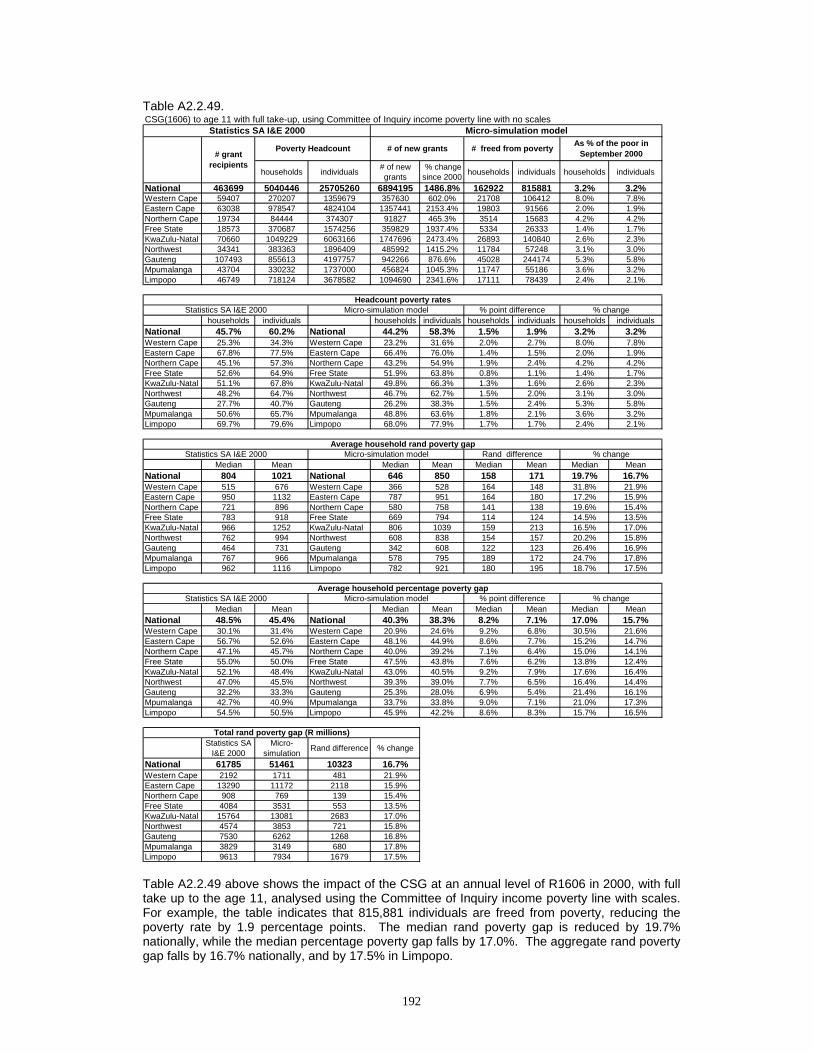
192
Table A2.2.49.
Table A2.2.49 above shows the impact of the CSG at an annual level of R1606 in 2000, with full take up to the age 11, analysed using the Committee of Inquiry income poverty line with scales. For example, the table indicates that 815,881 individuals are freed from poverty, reducing the poverty rate by 1.9 percentage points. The median rand poverty gap is reduced by 19.7% nationally, while the median percentage poverty gap falls by 17.0%. The aggregate rand poverty gap falls by 16.7% nationally, and by 17.5% in Limpopo.
CSG(1606) to age 11 with full take-up, using Committee of Inquiry income poverty line with no scales
households individuals # of new grants
% change since 2000 households individuals households individuals
National 463699 5040446 25705260 6894195 1486.8% 162922 815881 3.2% 3.2%Western Cape 59407 270207 1359679 357630 602.0% 21708 106412 8.0% 7.8%Eastern Cape 63038 978547 4824104 1357441 2153.4% 19803 91566 2.0% 1.9%Northern Cape 19734 84444 374307 91827 465.3% 3514 15683 4.2% 4.2%Free State 18573 370687 1574256 359829 1937.4% 5334 26333 1.4% 1.7%KwaZulu-Natal 70660 1049229 6063166 1747696 2473.4% 26893 140840 2.6% 2.3%Northwest 34341 383363 1896409 485992 1415.2% 11784 57248 3.1% 3.0%Gauteng 107493 855613 4197757 942266 876.6% 45028 244174 5.3% 5.8%Mpumalanga 43704 330232 1737000 456824 1045.3% 11747 55186 3.6% 3.2%Limpopo 46749 718124 3678582 1094690 2341.6% 17111 78439 2.4% 2.1%
households individuals households individuals households individuals households individualsNational 45.7% 60.2% National 44.2% 58.3% 1.5% 1.9% 3.2% 3.2%Western Cape 25.3% 34.3% Western Cape 23.2% 31.6% 2.0% 2.7% 8.0% 7.8%Eastern Cape 67.8% 77.5% Eastern Cape 66.4% 76.0% 1.4% 1.5% 2.0% 1.9%Northern Cape 45.1% 57.3% Northern Cape 43.2% 54.9% 1.9% 2.4% 4.2% 4.2%Free State 52.6% 64.9% Free State 51.9% 63.8% 0.8% 1.1% 1.4% 1.7%KwaZulu-Natal 51.1% 67.8% KwaZulu-Natal 49.8% 66.3% 1.3% 1.6% 2.6% 2.3%Northwest 48.2% 64.7% Northwest 46.7% 62.7% 1.5% 2.0% 3.1% 3.0%Gauteng 27.7% 40.7% Gauteng 26.2% 38.3% 1.5% 2.4% 5.3% 5.8%Mpumalanga 50.6% 65.7% Mpumalanga 48.8% 63.6% 1.8% 2.1% 3.6% 3.2%Limpopo 69.7% 79.6% Limpopo 68.0% 77.9% 1.7% 1.7% 2.4% 2.1%
Median Mean Median Mean Median Mean Median MeanNational 804 1021 National 646 850 158 171 19.7% 16.7%Western Cape 515 676 Western Cape 366 528 164 148 31.8% 21.9%Eastern Cape 950 1132 Eastern Cape 787 951 164 180 17.2% 15.9%Northern Cape 721 896 Northern Cape 580 758 141 138 19.6% 15.4%Free State 783 918 Free State 669 794 114 124 14.5% 13.5%KwaZulu-Natal 966 1252 KwaZulu-Natal 806 1039 159 213 16.5% 17.0%Northwest 762 994 Northwest 608 838 154 157 20.2% 15.8%Gauteng 464 731 Gauteng 342 608 122 123 26.4% 16.9%Mpumalanga 767 966 Mpumalanga 578 795 189 172 24.7% 17.8%Limpopo 962 1116 Limpopo 782 921 180 195 18.7% 17.5%
Median Mean Median Mean Median Mean Median MeanNational 48.5% 45.4% National 40.3% 38.3% 8.2% 7.1% 17.0% 15.7%Western Cape 30.1% 31.4% Western Cape 20.9% 24.6% 9.2% 6.8% 30.5% 21.6%Eastern Cape 56.7% 52.6% Eastern Cape 48.1% 44.9% 8.6% 7.7% 15.2% 14.7%Northern Cape 47.1% 45.7% Northern Cape 40.0% 39.2% 7.1% 6.4% 15.0% 14.1%Free State 55.0% 50.0% Free State 47.5% 43.8% 7.6% 6.2% 13.8% 12.4%KwaZulu-Natal 52.1% 48.4% KwaZulu-Natal 43.0% 40.5% 9.2% 7.9% 17.6% 16.4%Northwest 47.0% 45.5% Northwest 39.3% 39.0% 7.7% 6.5% 16.4% 14.4%Gauteng 32.2% 33.3% Gauteng 25.3% 28.0% 6.9% 5.4% 21.4% 16.1%Mpumalanga 42.7% 40.9% Mpumalanga 33.7% 33.8% 9.0% 7.1% 21.0% 17.3%Limpopo 54.5% 50.5% Limpopo 45.9% 42.2% 8.6% 8.3% 15.7% 16.5%
Statistics SA I&E 2000
Micro-simulation Rand difference % change
National 61785 51461 10323 16.7%Western Cape 2192 1711 481 21.9%Eastern Cape 13290 11172 2118 15.9%Northern Cape 908 769 139 15.4%Free State 4084 3531 553 13.5%KwaZulu-Natal 15764 13081 2683 17.0%Northwest 4574 3853 721 15.8%Gauteng 7530 6262 1268 16.8%Mpumalanga 3829 3149 680 17.8%Limpopo 9613 7934 1679 17.5%
Total rand poverty gap (R millions)
Statistics SA I&E 2000 Micro-simulation model
Micro-simulation modelStatistics SA I&E 2000
Poverty Headcount# grant
recipients
% point differenceAverage household percentage poverty gap
Average household rand poverty gap% change
% changeMicro-simulation model
% change
Headcount poverty rates
# of new grants # freed from poverty As % of the poor in September 2000
Statistics SA I&E 2000 % point difference
Statistics SA I&E 2000 Micro-simulation model Rand difference

193
Table A2.2.50.
Table A2.2.50 above shows the impact of the CSG at an annual level of R1606 in 2000, with full take up to the age 14, analysed using the Committee of Inquiry income poverty line with scales. For example, the table indicates that 1,067,308 individuals are freed from poverty, reducing the poverty rate by 2.5 percentage points. The median rand poverty gap is reduced by 25.6% nationally, while the median percentage poverty gap falls by 22.2%. The aggregate rand poverty gap falls by 21.8% nationally, and by 23.0% in Limpopo.
CSG(1606) to age 14 with full take-up, using Committee of Inquiry income poverty line with no scales
households individuals # of new grants
% change since 2000 households individuals households individuals
National 463699 5040446 25705260 9017270 1944.6% 213763 1067308 4.2% 4.2%Western Cape 59407 270207 1359679 447321 753.0% 26621 134192 9.9% 9.9%Eastern Cape 63038 978547 4824104 1806084 2865.1% 24228 113613 2.5% 2.4%Northern Cape 19734 84444 374307 115417 584.9% 4099 18996 4.9% 5.1%Free State 18573 370687 1574256 477388 2570.3% 7812 36558 2.1% 2.3%KwaZulu-Natal 70660 1049229 6063166 2261426 3200.4% 36940 192688 3.5% 3.2%Northwest 34341 383363 1896409 641431 1867.8% 17925 85701 4.7% 4.5%Gauteng 107493 855613 4197757 1221625 1136.5% 59248 312614 6.9% 7.4%Mpumalanga 43704 330232 1737000 607515 1390.1% 15647 75883 4.7% 4.4%Limpopo 46749 718124 3678582 1439063 3078.3% 21243 97063 3.0% 2.6%
households individuals households individuals households individuals households individualsNational 45.7% 60.2% National 43.8% 57.7% 1.9% 2.5% 4.2% 4.2%Western Cape 25.3% 34.3% Western Cape 22.8% 30.9% 2.5% 3.4% 9.9% 9.9%Eastern Cape 67.8% 77.5% Eastern Cape 66.1% 75.7% 1.7% 1.8% 2.5% 2.4%Northern Cape 45.1% 57.3% Northern Cape 42.9% 54.4% 2.2% 2.9% 4.9% 5.1%Free State 52.6% 64.9% Free State 51.5% 63.4% 1.1% 1.5% 2.1% 2.3%KwaZulu-Natal 51.1% 67.8% KwaZulu-Natal 49.3% 65.7% 1.8% 2.2% 3.5% 3.2%Northwest 48.2% 64.7% Northwest 45.9% 61.8% 2.3% 2.9% 4.7% 4.5%Gauteng 27.7% 40.7% Gauteng 25.8% 37.7% 1.9% 3.0% 6.9% 7.4%Mpumalanga 50.6% 65.7% Mpumalanga 48.2% 62.8% 2.4% 2.9% 4.7% 4.4%Limpopo 69.7% 79.6% Limpopo 67.6% 77.5% 2.1% 2.1% 3.0% 2.6%
Median Mean Median Mean Median Mean Median MeanNational 804 1021 National 598 799 206 222 25.6% 21.8%Western Cape 515 676 Western Cape 324 491 226 185 43.9% 27.3%Eastern Cape 950 1132 Eastern Cape 725 892 226 240 23.8% 21.2%Northern Cape 721 896 Northern Cape 547 723 174 173 24.1% 19.3%Free State 783 918 Free State 623 756 160 163 20.4% 17.7%KwaZulu-Natal 966 1252 KwaZulu-Natal 748 977 218 275 22.5% 22.0%Northwest 762 994 Northwest 568 788 195 207 25.6% 20.8%Gauteng 464 731 Gauteng 301 573 163 158 35.2% 21.6%Mpumalanga 767 966 Mpumalanga 532 740 235 227 30.7% 23.4%Limpopo 962 1116 Limpopo 727 859 235 256 24.4% 23.0%
Median Mean Median Mean Median Mean Median MeanNational 48.5% 45.4% National 37.8% 36.1% 10.8% 9.3% 22.2% 20.5%Western Cape 30.1% 31.4% Western Cape 19.0% 23.0% 11.1% 8.3% 37.0% 26.6%Eastern Cape 56.7% 52.6% Eastern Cape 44.9% 42.3% 11.9% 10.3% 20.9% 19.6%Northern Cape 47.1% 45.7% Northern Cape 38.8% 37.6% 8.3% 8.0% 17.7% 17.6%Free State 55.0% 50.0% Free State 45.9% 41.9% 9.1% 8.1% 16.6% 16.2%KwaZulu-Natal 52.1% 48.4% KwaZulu-Natal 40.7% 38.1% 11.4% 10.3% 21.9% 21.2%Northwest 47.0% 45.5% Northwest 37.9% 36.8% 9.2% 8.6% 19.5% 19.0%Gauteng 32.2% 33.3% Gauteng 23.1% 26.6% 9.0% 6.8% 28.1% 20.3%Mpumalanga 42.7% 40.9% Mpumalanga 30.7% 31.5% 12.0% 9.4% 28.1% 22.9%Limpopo 54.5% 50.5% Limpopo 41.9% 39.5% 12.6% 11.0% 23.1% 21.9%
Statistics SA I&E 2000
Micro-simulation Rand difference % change
National 61785 48328 13457 21.8%Western Cape 2192 1593 599 27.3%Eastern Cape 13290 10475 2815 21.2%Northern Cape 908 733 175 19.3%Free State 4084 3361 723 17.7%KwaZulu-Natal 15764 12303 3461 22.0%Northwest 4574 3623 951 20.8%Gauteng 7530 5904 1626 21.6%Mpumalanga 3829 2931 898 23.4%Limpopo 9613 7405 2208 23.0%
Total rand poverty gap (R millions)
Statistics SA I&E 2000 Micro-simulation model
Micro-simulation modelStatistics SA I&E 2000
Poverty Headcount# grant
recipients
% point differenceAverage household percentage poverty gap
Average household rand poverty gap% change
% changeMicro-simulation model
% change
Headcount poverty rates
# of new grants # freed from poverty As % of the poor in September 2000
Statistics SA I&E 2000 % point difference
Statistics SA I&E 2000 Micro-simulation model Rand difference

194
Table A2.2.51.
Table A2.2.51 above shows the impact of the CSG at an annual level of R1606 in 2000, with full take up to the age 16, analysed using the Committee of Inquiry income poverty line with scales. For example, the table indicates that 1,354,436 individuals are freed from poverty, reducing the poverty rate by 3.2 percentage points. The median rand poverty gap is reduced by 30.0% nationally, while the median percentage poverty gap falls by 25.5%. The aggregate rand poverty gap falls by 25.1% nationally, and by 26.6% in Limpopo.
CSG(1606) to age 16 with full take-up, using Committee of Inquiry income poverty line with no scales
households individuals # of new grants
% change since 2000 households individuals households individuals
National 463699 5040446 25705260 10425391 2248.3% 268423 1354436 5.3% 5.3%Western Cape 59407 270207 1359679 517005 870.3% 33426 171277 12.4% 12.6%Eastern Cape 63038 978547 4824104 2103551 3337.0% 30963 136253 3.2% 2.8%Northern Cape 19734 84444 374307 132813 673.0% 5045 23699 6.0% 6.3%Free State 18573 370687 1574256 560084 3015.6% 11421 56994 3.1% 3.6%KwaZulu-Natal 70660 1049229 6063166 2611909 3696.4% 46539 257172 4.4% 4.2%Northwest 34341 383363 1896409 743994 2166.5% 21301 102874 5.6% 5.4%Gauteng 107493 855613 4197757 1375524 1279.6% 72076 388708 8.4% 9.3%Mpumalanga 43704 330232 1737000 706884 1617.4% 19403 92862 5.9% 5.3%Limpopo 46749 718124 3678582 1673627 3580.0% 28249 124597 3.9% 3.4%
households individuals households individuals households individuals households individualsNational 45.7% 60.2% National 43.3% 57.0% 2.4% 3.2% 5.3% 5.3%Western Cape 25.3% 34.3% Western Cape 22.2% 30.0% 3.1% 4.3% 12.4% 12.6%Eastern Cape 67.8% 77.5% Eastern Cape 65.6% 75.3% 2.1% 2.2% 3.2% 2.8%Northern Cape 45.1% 57.3% Northern Cape 42.4% 53.7% 2.7% 3.6% 6.0% 6.3%Free State 52.6% 64.9% Free State 51.0% 62.6% 1.6% 2.3% 3.1% 3.6%KwaZulu-Natal 51.1% 67.8% KwaZulu-Natal 48.8% 65.0% 2.3% 2.9% 4.4% 4.2%Northwest 48.2% 64.7% Northwest 45.5% 61.2% 2.7% 3.5% 5.6% 5.4%Gauteng 27.7% 40.7% Gauteng 25.4% 36.9% 2.3% 3.8% 8.4% 9.3%Mpumalanga 50.6% 65.7% Mpumalanga 47.7% 62.2% 3.0% 3.5% 5.9% 5.3%Limpopo 69.7% 79.6% Limpopo 66.9% 76.9% 2.7% 2.7% 3.9% 3.4%
Median Mean Median Mean Median Mean Median MeanNational 804 1021 National 562 765 242 256 30.0% 25.1%Western Cape 515 676 Western Cape 295 463 260 213 50.5% 31.5%Eastern Cape 950 1132 Eastern Cape 691 854 260 278 27.3% 24.6%Northern Cape 721 896 Northern Cape 504 698 217 198 30.0% 22.1%Free State 783 918 Free State 604 728 179 190 22.9% 20.7%KwaZulu-Natal 966 1252 KwaZulu-Natal 697 936 269 316 27.9% 25.3%Northwest 762 994 Northwest 535 755 227 239 29.8% 24.1%Gauteng 464 731 Gauteng 294 553 170 177 36.6% 24.3%Mpumalanga 767 966 Mpumalanga 476 704 291 262 38.0% 27.2%Limpopo 962 1116 Limpopo 680 819 282 296 29.3% 26.6%
Median Mean Median Mean Median Mean Median MeanNational 48.5% 45.4% National 36.2% 34.6% 12.4% 10.8% 25.5% 23.7%Western Cape 30.1% 31.4% Western Cape 17.5% 21.9% 12.6% 9.5% 42.0% 30.2%Eastern Cape 56.7% 52.6% Eastern Cape 42.9% 40.6% 13.8% 12.1% 24.3% 23.0%Northern Cape 47.1% 45.7% Northern Cape 37.6% 36.5% 9.5% 9.2% 20.2% 20.1%Free State 55.0% 50.0% Free State 44.1% 40.5% 10.9% 9.6% 19.8% 19.1%KwaZulu-Natal 52.1% 48.4% KwaZulu-Natal 39.0% 36.5% 13.1% 11.9% 25.1% 24.5%Northwest 47.0% 45.5% Northwest 36.5% 35.5% 10.6% 10.0% 22.5% 22.0%Gauteng 32.2% 33.3% Gauteng 22.4% 25.7% 9.8% 7.6% 30.4% 22.8%Mpumalanga 42.7% 40.9% Mpumalanga 29.4% 30.0% 13.3% 10.9% 31.2% 26.6%Limpopo 54.5% 50.5% Limpopo 40.2% 37.7% 14.3% 12.8% 26.2% 25.4%
Statistics SA I&E 2000
Micro-simulation Rand difference % change
National 61785 46278 15507 25.1%Western Cape 2192 1502 690 31.5%Eastern Cape 13290 10024 3266 24.6%Northern Cape 908 707 201 22.1%Free State 4084 3238 846 20.7%KwaZulu-Natal 15764 11782 3983 25.3%Northwest 4574 3473 1102 24.1%Gauteng 7530 5704 1825 24.2%Mpumalanga 3829 2789 1040 27.2%Limpopo 9613 7059 2554 26.6%
Total rand poverty gap (R millions)
Statistics SA I&E 2000 Micro-simulation model
Micro-simulation modelStatistics SA I&E 2000
Poverty Headcount# grant
recipients
% point differenceAverage household percentage poverty gap
Average household rand poverty gap% change
% changeMicro-simulation model
% change
Headcount poverty rates
# of new grants # freed from poverty As % of the poor in September 2000
Statistics SA I&E 2000 % point difference
Statistics SA I&E 2000 Micro-simulation model Rand difference
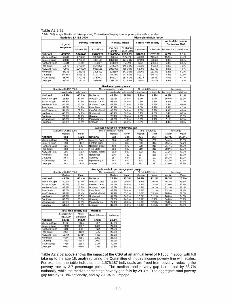
195
Table A2.2.52.
Table A2.2.52 above shows the impact of the CSG at an annual level of R1606 in 2000, with full take up to the age 18, analysed using the Committee of Inquiry income poverty line with scales. For example, the table indicates that 1,576,187 individuals are freed from poverty, reducing the poverty rate by 3.7 percentage points. The median rand poverty gap is reduced by 33.7% nationally, while the median percentage poverty gap falls by 29.3%. The aggregate rand poverty gap falls by 28.1% nationally, and by 29.8% in Limpopo.
CSG(1606) to age 18 with full take-up, using Committee of Inquiry income poverty line with no scales
households individuals # of new grants
% change since 2000 households individuals households individuals
National 463699 5040446 25705260 11749584 2533.9% 310039 1576187 6.2% 6.1%Western Cape 59407 270207 1359679 580674 977.5% 41933 215566 15.5% 15.9%Eastern Cape 63038 978547 4824104 2379870 3775.3% 37690 158608 3.9% 3.3%Northern Cape 19734 84444 374307 148080 750.4% 5355 24694 6.3% 6.6%Free State 18573 370687 1574256 648539 3491.8% 13931 66392 3.8% 4.2%KwaZulu-Natal 70660 1049229 6063166 2933091 4151.0% 51795 292762 4.9% 4.8%Northwest 34341 383363 1896409 828159 2411.6% 24369 117370 6.4% 6.2%Gauteng 107493 855613 4197757 1541023 1433.6% 80371 444740 9.4% 10.6%Mpumalanga 43704 330232 1737000 802024 1835.1% 23215 115857 7.0% 6.7%Limpopo 46749 718124 3678582 1888124 4038.9% 31380 140198 4.4% 3.8%
households individuals households individuals households individuals households individualsNational 45.7% 60.2% National 42.9% 56.5% 2.8% 3.7% 6.2% 6.1%Western Cape 25.3% 34.3% Western Cape 21.4% 28.8% 3.9% 5.4% 15.5% 15.9%Eastern Cape 67.8% 77.5% Eastern Cape 65.2% 74.9% 2.6% 2.5% 3.9% 3.3%Northern Cape 45.1% 57.3% Northern Cape 42.3% 53.6% 2.9% 3.8% 6.3% 6.6%Free State 52.6% 64.9% Free State 50.7% 62.2% 2.0% 2.7% 3.8% 4.2%KwaZulu-Natal 51.1% 67.8% KwaZulu-Natal 48.5% 64.6% 2.5% 3.3% 4.9% 4.8%Northwest 48.2% 64.7% Northwest 45.1% 60.7% 3.1% 4.0% 6.4% 6.2%Gauteng 27.7% 40.7% Gauteng 25.1% 36.4% 2.6% 4.3% 9.4% 10.6%Mpumalanga 50.6% 65.7% Mpumalanga 47.0% 61.3% 3.6% 4.4% 7.1% 6.7%Limpopo 69.7% 79.6% Limpopo 66.6% 76.6% 3.0% 3.0% 4.4% 3.8%
Median Mean Median Mean Median Mean Median MeanNational 804 1021 National 533 734 271 287 33.7% 28.1%Western Cape 515 676 Western Cape 266 439 280 237 54.4% 35.0%Eastern Cape 950 1132 Eastern Cape 671 818 280 314 29.4% 27.7%Northern Cape 721 896 Northern Cape 493 677 228 219 31.7% 24.5%Free State 783 918 Free State 563 699 219 219 28.0% 23.9%KwaZulu-Natal 966 1252 KwaZulu-Natal 663 899 303 353 31.3% 28.2%Northwest 762 994 Northwest 506 729 257 266 33.7% 26.7%Gauteng 464 731 Gauteng 287 534 177 197 38.1% 27.0%Mpumalanga 767 966 Mpumalanga 444 670 324 297 42.2% 30.7%Limpopo 962 1116 Limpopo 645 783 317 332 33.0% 29.8%
Median Mean Median Mean Median Mean Median MeanNational 48.5% 45.4% National 34.3% 33.3% 14.2% 12.1% 29.3% 26.7%Western Cape 30.1% 31.4% Western Cape 16.5% 20.9% 13.6% 10.5% 45.2% 33.5%Eastern Cape 56.7% 52.6% Eastern Cape 41.4% 38.9% 15.3% 13.8% 27.0% 26.1%Northern Cape 47.1% 45.7% Northern Cape 36.6% 35.4% 10.5% 10.2% 22.3% 22.4%Free State 55.0% 50.0% Free State 42.2% 38.8% 12.8% 11.2% 23.3% 22.4%KwaZulu-Natal 52.1% 48.4% KwaZulu-Natal 37.1% 35.1% 15.0% 13.3% 28.8% 27.5%Northwest 47.0% 45.5% Northwest 34.8% 34.3% 12.2% 11.2% 26.0% 24.5%Gauteng 32.2% 33.3% Gauteng 21.2% 24.9% 10.9% 8.4% 34.0% 25.2%Mpumalanga 42.7% 40.9% Mpumalanga 27.4% 28.6% 15.3% 12.3% 35.8% 30.0%Limpopo 54.5% 50.5% Limpopo 37.8% 36.0% 16.8% 14.5% 30.7% 28.6%
Statistics SA I&E 2000
Micro-simulation Rand difference % change
National 61785 44399 17386 28.1%Western Cape 2192 1425 767 35.0%Eastern Cape 13290 9607 3683 27.7%Northern Cape 908 686 222 24.5%Free State 4084 3109 975 23.9%KwaZulu-Natal 15764 11314 4450 28.2%Northwest 4574 3351 1223 26.7%Gauteng 7530 5503 2027 26.9%Mpumalanga 3829 2653 1176 30.7%Limpopo 9613 6750 2863 29.8%
Total rand poverty gap (R millions)
Statistics SA I&E 2000 Micro-simulation model
Micro-simulation modelStatistics SA I&E 2000
Poverty Headcount# grant
recipients
% point differenceAverage household percentage poverty gap
Average household rand poverty gap% change
% changeMicro-simulation model
% change
Headcount poverty rates
# of new grants # freed from poverty As % of the poor in September 2000
Statistics SA I&E 2000 % point difference
Statistics SA I&E 2000 Micro-simulation model Rand difference
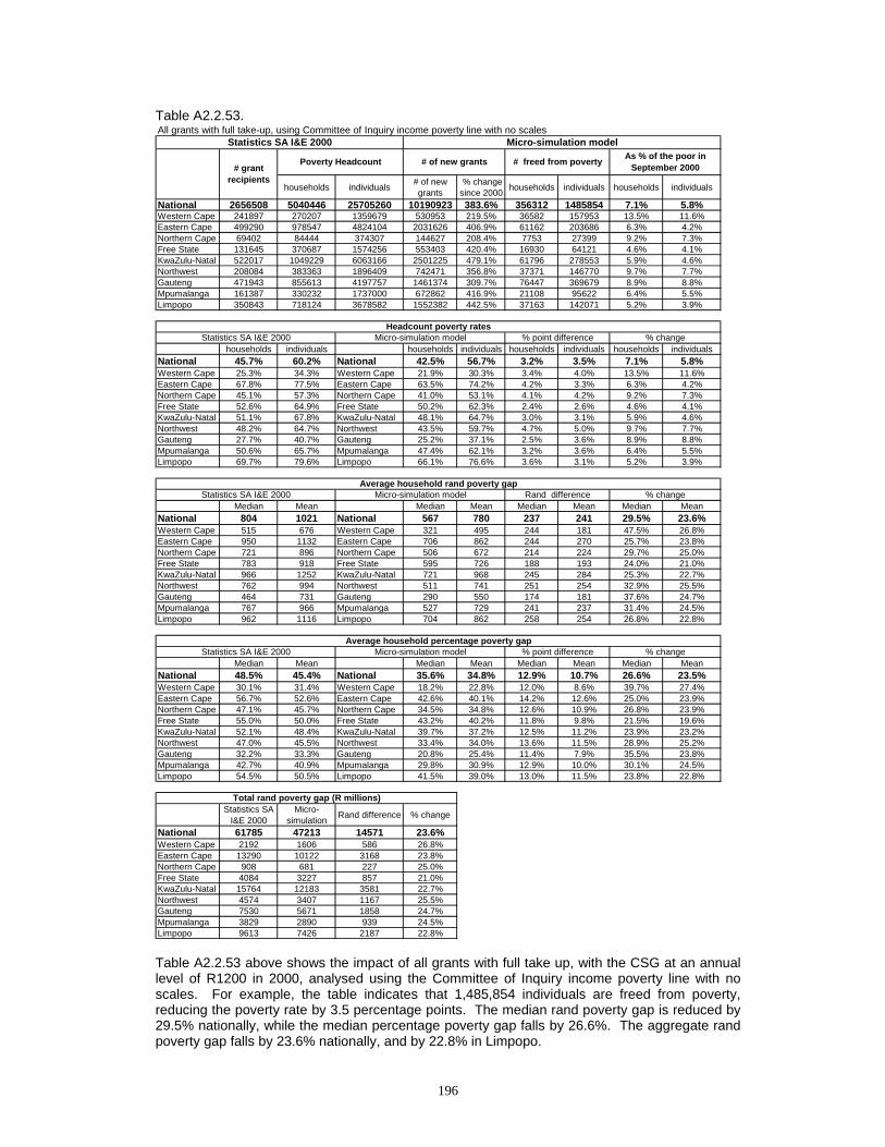
196
Table A2.2.53.
Table A2.2.53 above shows the impact of all grants with full take up, with the CSG at an annual level of R1200 in 2000, analysed using the Committee of Inquiry income poverty line with no scales. For example, the table indicates that 1,485,854 individuals are freed from poverty, reducing the poverty rate by 3.5 percentage points. The median rand poverty gap is reduced by 29.5% nationally, while the median percentage poverty gap falls by 26.6%. The aggregate rand poverty gap falls by 23.6% nationally, and by 22.8% in Limpopo.
All grants with full take-up, using Committee of Inquiry income poverty line with no scales
households individuals # of new grants
% change since 2000 households individuals households individuals
National 2656508 5040446 25705260 10190923 383.6% 356312 1485854 7.1% 5.8%Western Cape 241897 270207 1359679 530953 219.5% 36582 157953 13.5% 11.6%Eastern Cape 499290 978547 4824104 2031626 406.9% 61162 203686 6.3% 4.2%Northern Cape 69402 84444 374307 144627 208.4% 7753 27399 9.2% 7.3%Free State 131645 370687 1574256 553403 420.4% 16930 64121 4.6% 4.1%KwaZulu-Natal 522017 1049229 6063166 2501225 479.1% 61796 278553 5.9% 4.6%Northwest 208084 383363 1896409 742471 356.8% 37371 146770 9.7% 7.7%Gauteng 471943 855613 4197757 1461374 309.7% 76447 369679 8.9% 8.8%Mpumalanga 161387 330232 1737000 672862 416.9% 21108 95622 6.4% 5.5%Limpopo 350843 718124 3678582 1552382 442.5% 37163 142071 5.2% 3.9%
households individuals households individuals households individuals households individualsNational 45.7% 60.2% National 42.5% 56.7% 3.2% 3.5% 7.1% 5.8%Western Cape 25.3% 34.3% Western Cape 21.9% 30.3% 3.4% 4.0% 13.5% 11.6%Eastern Cape 67.8% 77.5% Eastern Cape 63.5% 74.2% 4.2% 3.3% 6.3% 4.2%Northern Cape 45.1% 57.3% Northern Cape 41.0% 53.1% 4.1% 4.2% 9.2% 7.3%Free State 52.6% 64.9% Free State 50.2% 62.3% 2.4% 2.6% 4.6% 4.1%KwaZulu-Natal 51.1% 67.8% KwaZulu-Natal 48.1% 64.7% 3.0% 3.1% 5.9% 4.6%Northwest 48.2% 64.7% Northwest 43.5% 59.7% 4.7% 5.0% 9.7% 7.7%Gauteng 27.7% 40.7% Gauteng 25.2% 37.1% 2.5% 3.6% 8.9% 8.8%Mpumalanga 50.6% 65.7% Mpumalanga 47.4% 62.1% 3.2% 3.6% 6.4% 5.5%Limpopo 69.7% 79.6% Limpopo 66.1% 76.6% 3.6% 3.1% 5.2% 3.9%
Median Mean Median Mean Median Mean Median MeanNational 804 1021 National 567 780 237 241 29.5% 23.6%Western Cape 515 676 Western Cape 321 495 244 181 47.5% 26.8%Eastern Cape 950 1132 Eastern Cape 706 862 244 270 25.7% 23.8%Northern Cape 721 896 Northern Cape 506 672 214 224 29.7% 25.0%Free State 783 918 Free State 595 726 188 193 24.0% 21.0%KwaZulu-Natal 966 1252 KwaZulu-Natal 721 968 245 284 25.3% 22.7%Northwest 762 994 Northwest 511 741 251 254 32.9% 25.5%Gauteng 464 731 Gauteng 290 550 174 181 37.6% 24.7%Mpumalanga 767 966 Mpumalanga 527 729 241 237 31.4% 24.5%Limpopo 962 1116 Limpopo 704 862 258 254 26.8% 22.8%
Median Mean Median Mean Median Mean Median MeanNational 48.5% 45.4% National 35.6% 34.8% 12.9% 10.7% 26.6% 23.5%Western Cape 30.1% 31.4% Western Cape 18.2% 22.8% 12.0% 8.6% 39.7% 27.4%Eastern Cape 56.7% 52.6% Eastern Cape 42.6% 40.1% 14.2% 12.6% 25.0% 23.9%Northern Cape 47.1% 45.7% Northern Cape 34.5% 34.8% 12.6% 10.9% 26.8% 23.9%Free State 55.0% 50.0% Free State 43.2% 40.2% 11.8% 9.8% 21.5% 19.6%KwaZulu-Natal 52.1% 48.4% KwaZulu-Natal 39.7% 37.2% 12.5% 11.2% 23.9% 23.2%Northwest 47.0% 45.5% Northwest 33.4% 34.0% 13.6% 11.5% 28.9% 25.2%Gauteng 32.2% 33.3% Gauteng 20.8% 25.4% 11.4% 7.9% 35.5% 23.8%Mpumalanga 42.7% 40.9% Mpumalanga 29.8% 30.9% 12.9% 10.0% 30.1% 24.5%Limpopo 54.5% 50.5% Limpopo 41.5% 39.0% 13.0% 11.5% 23.8% 22.8%
Statistics SA I&E 2000
Micro-simulation Rand difference % change
National 61785 47213 14571 23.6%Western Cape 2192 1606 586 26.8%Eastern Cape 13290 10122 3168 23.8%Northern Cape 908 681 227 25.0%Free State 4084 3227 857 21.0%KwaZulu-Natal 15764 12183 3581 22.7%Northwest 4574 3407 1167 25.5%Gauteng 7530 5671 1858 24.7%Mpumalanga 3829 2890 939 24.5%Limpopo 9613 7426 2187 22.8%
Total rand poverty gap (R millions)
Statistics SA I&E 2000 Micro-simulation model
Micro-simulation modelStatistics SA I&E 2000
Poverty Headcount# grant
recipients
% point differenceAverage household percentage poverty gap
Average household rand poverty gap% change
% changeMicro-simulation model
% change
Headcount poverty rates
# of new grants # freed from poverty As % of the poor in September 2000
Statistics SA I&E 2000 % point difference
Statistics SA I&E 2000 Micro-simulation model Rand difference

197
Table A2.2.54.
Table A2.2.54 above shows the impact of all grants with full take up, with the CSG at an annual level of R1606 in 2000, analysed using the Committee of Inquiry income poverty line with no scales. For example, the table indicates that 1,817,450 individuals are freed from poverty, reducing the poverty rate by 4.3 percentage points. The median rand poverty gap is reduced by 35.8% nationally, while the median percentage poverty gap falls by 32.3%. The aggregate rand poverty gap falls by 28.9% nationally, and by 28.4% in Limpopo.
All grants(1606) with full take-up, using Committee of Inquiry income poverty line with no scales
households individuals # of new grants
% change since 2000 households individuals households individuals
National 2656508 5040446 25705260 10190923 383.6% 423265 1817450 8.4% 7.1%Western Cape 241897 270207 1359679 530953 219.5% 41238 183711 15.3% 13.5%Eastern Cape 499290 978547 4824104 2031626 406.9% 71181 249613 7.3% 5.2%Northern Cape 69402 84444 374307 144627 208.4% 9318 34190 11.0% 9.1%Free State 131645 370687 1574256 553403 420.4% 19997 78088 5.4% 5.0%KwaZulu-Natal 522017 1049229 6063166 2501225 479.1% 74180 338408 7.1% 5.6%Northwest 208084 383363 1896409 742471 356.8% 42983 174546 11.2% 9.2%Gauteng 471943 855613 4197757 1461374 309.7% 93624 465008 10.9% 11.1%Mpumalanga 161387 330232 1737000 672862 416.9% 26237 120976 7.9% 7.0%Limpopo 350843 718124 3678582 1552382 442.5% 44507 172910 6.2% 4.7%
households individuals households individuals households individuals households individualsNational 45.7% 60.2% National 41.9% 55.9% 3.8% 4.3% 8.4% 7.1%Western Cape 25.3% 34.3% Western Cape 21.4% 29.6% 3.9% 4.6% 15.3% 13.5%Eastern Cape 67.8% 77.5% Eastern Cape 62.8% 73.5% 4.9% 4.0% 7.3% 5.2%Northern Cape 45.1% 57.3% Northern Cape 40.1% 52.1% 5.0% 5.2% 11.0% 9.1%Free State 52.6% 64.9% Free State 49.8% 61.7% 2.8% 3.2% 5.4% 5.0%KwaZulu-Natal 51.1% 67.8% KwaZulu-Natal 47.5% 64.0% 3.6% 3.8% 7.1% 5.6%Northwest 48.2% 64.7% Northwest 42.8% 58.7% 5.4% 6.0% 11.2% 9.2%Gauteng 27.7% 40.7% Gauteng 24.7% 36.2% 3.0% 4.5% 10.9% 11.1%Mpumalanga 50.6% 65.7% Mpumalanga 46.6% 61.1% 4.0% 4.6% 7.9% 7.0%Limpopo 69.7% 79.6% Limpopo 65.4% 75.9% 4.3% 3.7% 6.2% 4.7%
Median Mean Median Mean Median Mean Median MeanNational 804 1021 National 517 726 288 295 35.8% 28.9%Western Cape 515 676 Western Cape 264 452 300 224 58.3% 33.1%Eastern Cape 950 1132 Eastern Cape 650 803 300 328 31.6% 29.0%Northern Cape 721 896 Northern Cape 455 630 266 266 36.9% 29.7%Free State 783 918 Free State 561 686 222 232 28.3% 25.3%KwaZulu-Natal 966 1252 KwaZulu-Natal 651 900 314 352 32.6% 28.1%Northwest 762 994 Northwest 464 691 298 303 39.1% 30.5%Gauteng 464 731 Gauteng 250 514 214 217 46.1% 29.7%Mpumalanga 767 966 Mpumalanga 461 675 306 291 39.9% 30.1%Limpopo 962 1116 Limpopo 648 799 314 317 32.6% 28.4%
Median Mean Median Mean Median Mean Median MeanNational 48.5% 45.4% National 32.9% 32.5% 15.7% 12.9% 32.3% 28.4%Western Cape 30.1% 31.4% Western Cape 16.3% 20.9% 13.8% 10.5% 45.8% 33.5%Eastern Cape 56.7% 52.6% Eastern Cape 39.4% 37.6% 17.3% 15.1% 30.5% 28.6%Northern Cape 47.1% 45.7% Northern Cape 32.2% 32.9% 14.9% 12.8% 31.6% 28.1%Free State 55.0% 50.0% Free State 40.5% 38.3% 14.5% 11.7% 26.4% 23.5%KwaZulu-Natal 52.1% 48.4% KwaZulu-Natal 36.5% 34.7% 15.6% 13.7% 29.9% 28.3%Northwest 47.0% 45.5% Northwest 30.8% 32.0% 16.2% 13.5% 34.5% 29.7%Gauteng 32.2% 33.3% Gauteng 18.8% 23.9% 13.4% 9.5% 41.6% 28.4%Mpumalanga 42.7% 40.9% Mpumalanga 26.8% 28.6% 15.9% 12.2% 37.1% 29.9%Limpopo 54.5% 50.5% Limpopo 38.2% 36.3% 16.3% 14.2% 30.0% 28.1%
Statistics SA I&E 2000
Micro-simulation Rand difference % change
National 61785 43957 17828 28.9%Western Cape 2192 1466 726 33.1%Eastern Cape 13290 9435 3855 29.0%Northern Cape 908 639 269 29.7%Free State 4084 3052 1032 25.3%KwaZulu-Natal 15764 11333 4432 28.1%Northwest 4574 3179 1395 30.5%Gauteng 7530 5297 2233 29.7%Mpumalanga 3829 2675 1154 30.1%Limpopo 9613 6882 2731 28.4%
Total rand poverty gap (R millions)
Statistics SA I&E 2000 Micro-simulation model
Micro-simulation modelStatistics SA I&E 2000
Poverty Headcount# grant
recipients
% point differenceAverage household percentage poverty gap
Average household rand poverty gap% change
% changeMicro-simulation model
% change
Headcount poverty rates
# of new grants # freed from poverty As % of the poor in September 2000
Statistics SA I&E 2000 % point difference
Statistics SA I&E 2000 Micro-simulation model Rand difference
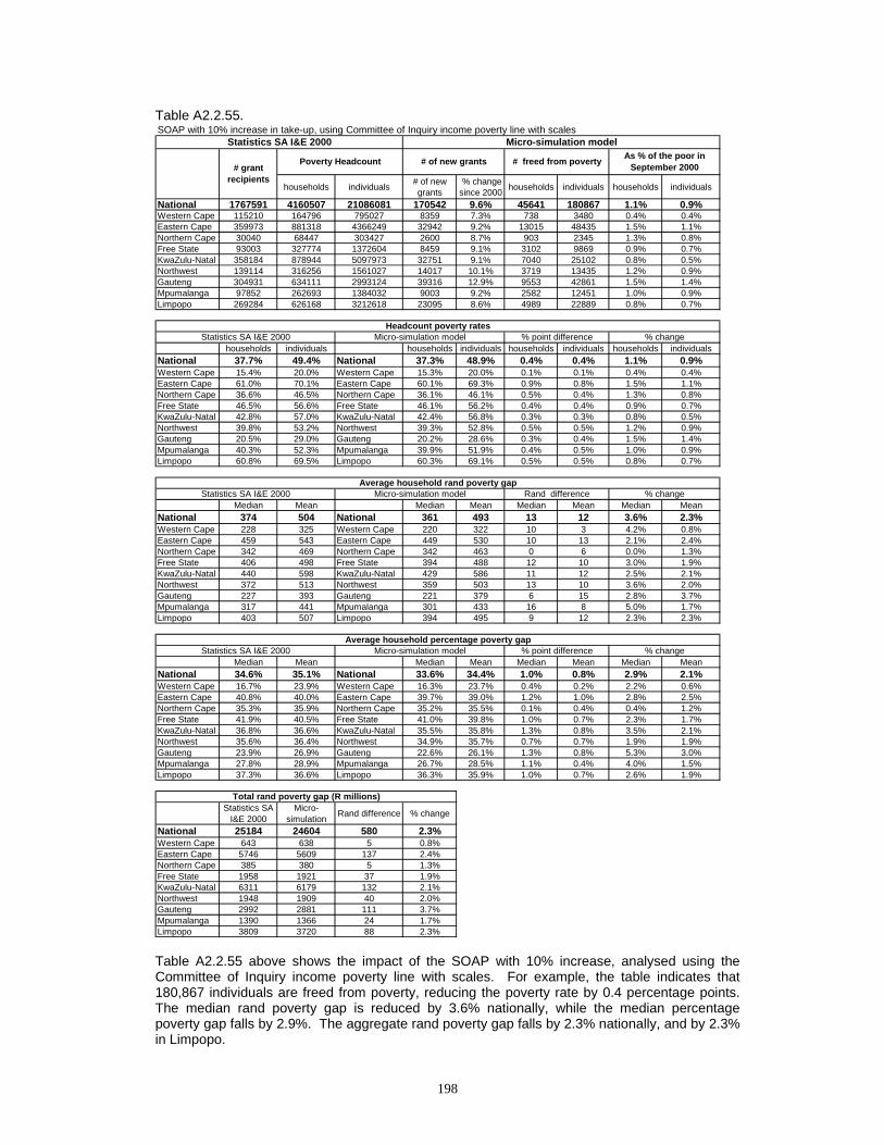
198
Table A2.2.55.
Table A2.2.55 above shows the impact of the SOAP with 10% increase, analysed using the Committee of Inquiry income poverty line with scales. For example, the table indicates that 180,867 individuals are freed from poverty, reducing the poverty rate by 0.4 percentage points. The median rand poverty gap is reduced by 3.6% nationally, while the median percentage poverty gap falls by 2.9%. The aggregate rand poverty gap falls by 2.3% nationally, and by 2.3% in Limpopo.
SOAP with 10% increase in take-up, using Committee of Inquiry income poverty line with scales
households individuals # of new grants
% change since 2000 households individuals households individuals
National 1767591 4160507 21086081 170542 9.6% 45641 180867 1.1% 0.9%Western Cape 115210 164796 795027 8359 7.3% 738 3480 0.4% 0.4%Eastern Cape 359973 881318 4366249 32942 9.2% 13015 48435 1.5% 1.1%Northern Cape 30040 68447 303427 2600 8.7% 903 2345 1.3% 0.8%Free State 93003 327774 1372604 8459 9.1% 3102 9869 0.9% 0.7%KwaZulu-Natal 358184 878944 5097973 32751 9.1% 7040 25102 0.8% 0.5%Northwest 139114 316256 1561027 14017 10.1% 3719 13435 1.2% 0.9%Gauteng 304931 634111 2993124 39316 12.9% 9553 42861 1.5% 1.4%Mpumalanga 97852 262693 1384032 9003 9.2% 2582 12451 1.0% 0.9%Limpopo 269284 626168 3212618 23095 8.6% 4989 22889 0.8% 0.7%
households individuals households individuals households individuals households individualsNational 37.7% 49.4% National 37.3% 48.9% 0.4% 0.4% 1.1% 0.9%Western Cape 15.4% 20.0% Western Cape 15.3% 20.0% 0.1% 0.1% 0.4% 0.4%Eastern Cape 61.0% 70.1% Eastern Cape 60.1% 69.3% 0.9% 0.8% 1.5% 1.1%Northern Cape 36.6% 46.5% Northern Cape 36.1% 46.1% 0.5% 0.4% 1.3% 0.8%Free State 46.5% 56.6% Free State 46.1% 56.2% 0.4% 0.4% 0.9% 0.7%KwaZulu-Natal 42.8% 57.0% KwaZulu-Natal 42.4% 56.8% 0.3% 0.3% 0.8% 0.5%Northwest 39.8% 53.2% Northwest 39.3% 52.8% 0.5% 0.5% 1.2% 0.9%Gauteng 20.5% 29.0% Gauteng 20.2% 28.6% 0.3% 0.4% 1.5% 1.4%Mpumalanga 40.3% 52.3% Mpumalanga 39.9% 51.9% 0.4% 0.5% 1.0% 0.9%Limpopo 60.8% 69.5% Limpopo 60.3% 69.1% 0.5% 0.5% 0.8% 0.7%
Median Mean Median Mean Median Mean Median MeanNational 374 504 National 361 493 13 12 3.6% 2.3%Western Cape 228 325 Western Cape 220 322 10 3 4.2% 0.8%Eastern Cape 459 543 Eastern Cape 449 530 10 13 2.1% 2.4%Northern Cape 342 469 Northern Cape 342 463 0 6 0.0% 1.3%Free State 406 498 Free State 394 488 12 10 3.0% 1.9%KwaZulu-Natal 440 598 KwaZulu-Natal 429 586 11 12 2.5% 2.1%Northwest 372 513 Northwest 359 503 13 10 3.6% 2.0%Gauteng 227 393 Gauteng 221 379 6 15 2.8% 3.7%Mpumalanga 317 441 Mpumalanga 301 433 16 8 5.0% 1.7%Limpopo 403 507 Limpopo 394 495 9 12 2.3% 2.3%
Median Mean Median Mean Median Mean Median MeanNational 34.6% 35.1% National 33.6% 34.4% 1.0% 0.8% 2.9% 2.1%Western Cape 16.7% 23.9% Western Cape 16.3% 23.7% 0.4% 0.2% 2.2% 0.6%Eastern Cape 40.8% 40.0% Eastern Cape 39.7% 39.0% 1.2% 1.0% 2.8% 2.5%Northern Cape 35.3% 35.9% Northern Cape 35.2% 35.5% 0.1% 0.4% 0.4% 1.2%Free State 41.9% 40.5% Free State 41.0% 39.8% 1.0% 0.7% 2.3% 1.7%KwaZulu-Natal 36.8% 36.6% KwaZulu-Natal 35.5% 35.8% 1.3% 0.8% 3.5% 2.1%Northwest 35.6% 36.4% Northwest 34.9% 35.7% 0.7% 0.7% 1.9% 1.9%Gauteng 23.9% 26.9% Gauteng 22.6% 26.1% 1.3% 0.8% 5.3% 3.0%Mpumalanga 27.8% 28.9% Mpumalanga 26.7% 28.5% 1.1% 0.4% 4.0% 1.5%Limpopo 37.3% 36.6% Limpopo 36.3% 35.9% 1.0% 0.7% 2.6% 1.9%
Statistics SA I&E 2000
Micro-simulation Rand difference % change
National 25184 24604 580 2.3%Western Cape 643 638 5 0.8%Eastern Cape 5746 5609 137 2.4%Northern Cape 385 380 5 1.3%Free State 1958 1921 37 1.9%KwaZulu-Natal 6311 6179 132 2.1%Northwest 1948 1909 40 2.0%Gauteng 2992 2881 111 3.7%Mpumalanga 1390 1366 24 1.7%Limpopo 3809 3720 88 2.3%
% change
Headcount poverty rates
# of new grants # freed from poverty As % of the poor in September 2000
Statistics SA I&E 2000 % point difference
Statistics SA I&E 2000 Micro-simulation model Rand differenceAverage household rand poverty gap
% change
% changeMicro-simulation model
Total rand poverty gap (R millions)
Statistics SA I&E 2000 Micro-simulation model
Micro-simulation modelStatistics SA I&E 2000
Poverty Headcount# grant
recipients
% point differenceAverage household percentage poverty gap

199
Table A2.2.56.
Table A2.2.56 above shows the impact of the SOAP with full take up, analysed using the Committee of Inquiry income poverty line with scales. For example, the table indicates that 385,185 individuals are freed from poverty, reducing the poverty rate by 0.9 percentage points. The median rand poverty gap is reduced by 6.8% nationally, while the median percentage poverty gap falls by 5.4%. The aggregate rand poverty gap falls by 4.5% nationally, and by 3.6% in Limpopo.
SOAP with full take-up, using Committee of Inquiry income poverty line with scales
households individuals # of new grants
% change since 2000 households individuals households individuals
National 1767591 4160507 21086081 417730 23.6% 98489 385185 2.4% 1.8%Western Cape 115210 164796 795027 28838 25.0% 5982 14471 3.6% 1.8%Eastern Cape 359973 881318 4366249 80962 22.5% 28305 106706 3.2% 2.4%Northern Cape 30040 68447 303427 7490 24.9% 1688 4300 2.5% 1.4%Free State 93003 327774 1372604 22720 24.4% 7289 30231 2.2% 2.2%KwaZulu-Natal 358184 878944 5097973 87472 24.4% 17645 63344 2.0% 1.2%Northwest 139114 316256 1561027 28155 20.2% 8397 37099 2.7% 2.4%Gauteng 304931 634111 2993124 109732 36.0% 15668 71664 2.5% 2.4%Mpumalanga 97852 262693 1384032 12845 13.1% 3084 14459 1.2% 1.0%Limpopo 269284 626168 3212618 39516 14.7% 10431 42911 1.7% 1.3%
households individuals households individuals households individuals households individualsNational 37.7% 49.4% National 36.8% 48.5% 0.9% 0.9% 2.4% 1.8%Western Cape 15.4% 20.0% Western Cape 14.9% 19.7% 0.6% 0.4% 3.6% 1.8%Eastern Cape 61.0% 70.1% Eastern Cape 59.1% 68.4% 2.0% 1.7% 3.2% 2.4%Northern Cape 36.6% 46.5% Northern Cape 35.7% 45.8% 0.9% 0.7% 2.5% 1.4%Free State 46.5% 56.6% Free State 45.5% 55.3% 1.0% 1.2% 2.2% 2.2%KwaZulu-Natal 42.8% 57.0% KwaZulu-Natal 41.9% 56.3% 0.9% 0.7% 2.0% 1.2%Northwest 39.8% 53.2% Northwest 38.7% 52.0% 1.1% 1.3% 2.7% 2.4%Gauteng 20.5% 29.0% Gauteng 20.0% 28.3% 0.5% 0.7% 2.5% 2.4%Mpumalanga 40.3% 52.3% Mpumalanga 39.8% 51.8% 0.5% 0.5% 1.2% 1.0%Limpopo 60.8% 69.5% Limpopo 59.8% 68.6% 1.0% 0.9% 1.7% 1.3%
Median Mean Median Mean Median Mean Median MeanNational 374 504 National 349 482 25 23 6.8% 4.5%Western Cape 228 325 Western Cape 211 318 27 7 11.7% 2.0%Eastern Cape 459 543 Eastern Cape 432 516 27 27 5.8% 5.0%Northern Cape 342 469 Northern Cape 339 454 3 15 0.9% 3.1%Free State 406 498 Free State 390 476 16 22 4.0% 4.4%KwaZulu-Natal 440 598 KwaZulu-Natal 410 571 31 27 7.0% 4.5%Northwest 372 513 Northwest 344 492 28 22 7.5% 4.2%Gauteng 227 393 Gauteng 210 367 17 26 7.6% 6.6%Mpumalanga 317 441 Mpumalanga 300 431 17 10 5.4% 2.3%Limpopo 403 507 Limpopo 382 489 20 18 5.0% 3.6%
Median Mean Median Mean Median Mean Median MeanNational 34.6% 35.1% National 32.8% 33.6% 1.9% 1.5% 5.4% 4.3%Western Cape 16.7% 23.9% Western Cape 15.5% 23.0% 1.2% 0.8% 7.1% 3.5%Eastern Cape 40.8% 40.0% Eastern Cape 38.3% 37.9% 2.6% 2.0% 6.3% 5.1%Northern Cape 35.3% 35.9% Northern Cape 34.3% 34.8% 1.1% 1.1% 3.0% 3.1%Free State 41.9% 40.5% Free State 40.1% 38.9% 1.8% 1.5% 4.3% 3.8%KwaZulu-Natal 36.8% 36.6% KwaZulu-Natal 34.3% 34.8% 2.5% 1.7% 6.8% 4.7%Northwest 35.6% 36.4% Northwest 34.1% 34.9% 1.5% 1.5% 4.2% 4.1%Gauteng 23.9% 26.9% Gauteng 21.6% 25.6% 2.3% 1.4% 9.6% 5.1%Mpumalanga 27.8% 28.9% Mpumalanga 26.2% 28.3% 1.6% 0.6% 5.7% 2.0%Limpopo 37.3% 36.6% Limpopo 35.7% 35.4% 1.6% 1.2% 4.3% 3.3%
Statistics SA I&E 2000
Micro-simulation Rand difference % change
National 25184 24059 1126 4.5%Western Cape 643 630 13 2.0%Eastern Cape 5746 5460 286 5.0%Northern Cape 385 373 12 3.1%Free State 1958 1873 86 4.4%KwaZulu-Natal 6311 6027 283 4.5%Northwest 1948 1866 82 4.2%Gauteng 2992 2796 196 6.6%Mpumalanga 1390 1358 31 2.3%Limpopo 3809 3673 135 3.6%
% change
Headcount poverty rates
# of new grants # freed from poverty As % of the poor in September 2000
Statistics SA I&E 2000 % point difference
Statistics SA I&E 2000 Micro-simulation model Rand differenceAverage household rand poverty gap
% change
% changeMicro-simulation model
Total rand poverty gap (R millions)
Statistics SA I&E 2000 Micro-simulation model
Micro-simulation modelStatistics SA I&E 2000
Poverty Headcount# grant
recipients
% point differenceAverage household percentage poverty gap
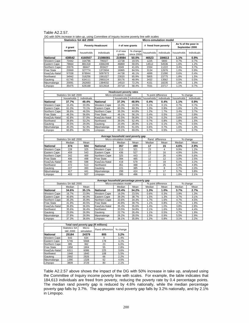
200
Table A2.2.57.
Table A2.2.57 above shows the impact of the DG with 50% increase in take up, analysed using the Committee of Inquiry income poverty line with scales. For example, the table indicates that 184,613 individuals are freed from poverty, reducing the poverty rate by 0.4 percentage points. The median rand poverty gap is reduced by 4.6% nationally, while the median percentage poverty gap falls by 3.7%. The aggregate rand poverty gap falls by 3.2% nationally, and by 2.1% in Limpopo.
DG with 50% increase in take-up, using Committee of Inquiry income poverty line with scales
households individuals # of new grants
% change since 2000 households individuals households individuals
National 438542 4160507 21086081 219084 50.0% 46523 184613 1.1% 0.9%Western Cape 70442 164796 795027 13738 19.5% 1225 5800 0.7% 0.7%Eastern Cape 78664 881318 4366249 46869 59.6% 14512 54536 1.6% 1.2%Northern Cape 20076 68447 303427 8349 41.6% 2334 11222 3.4% 3.7%Free State 20069 327774 1372604 16965 84.5% 3134 12676 1.0% 0.9%KwaZulu-Natal 97038 878944 5097973 44738 46.1% 4899 21090 0.6% 0.4%Northwest 34942 316256 1561027 23020 65.9% 5805 23775 1.8% 1.5%Gauteng 61745 634111 2993124 30176 48.9% 3432 13562 0.5% 0.5%Mpumalanga 20091 262693 1384032 14510 72.2% 4151 18235 1.6% 1.3%Limpopo 35475 626168 3212618 20719 58.4% 7031 23717 1.1% 0.7%
households individuals households individuals households individuals households individualsNational 37.7% 49.4% National 37.3% 48.9% 0.4% 0.4% 1.1% 0.9%Western Cape 15.4% 20.0% Western Cape 15.3% 19.9% 0.1% 0.1% 0.7% 0.7%Eastern Cape 61.0% 70.1% Eastern Cape 60.0% 69.3% 1.0% 0.9% 1.6% 1.2%Northern Cape 36.6% 46.5% Northern Cape 35.3% 44.8% 1.2% 1.7% 3.4% 3.7%Free State 46.5% 56.6% Free State 46.1% 56.1% 0.4% 0.5% 1.0% 0.9%KwaZulu-Natal 42.8% 57.0% KwaZulu-Natal 42.5% 56.8% 0.2% 0.2% 0.6% 0.4%Northwest 39.8% 53.2% Northwest 39.0% 52.4% 0.7% 0.8% 1.8% 1.5%Gauteng 20.5% 29.0% Gauteng 20.4% 28.9% 0.1% 0.1% 0.7% 0.5%Mpumalanga 40.3% 52.3% Mpumalanga 39.6% 51.6% 0.6% 0.7% 1.6% 1.3%Limpopo 60.8% 69.5% Limpopo 60.1% 69.0% 0.7% 0.5% 1.1% 0.7%
Median Mean Median Mean Median Mean Median MeanNational 374 504 National 357 490 17 15 4.6% 2.9%Western Cape 228 325 Western Cape 213 321 23 4 9.9% 1.2%Eastern Cape 459 543 Eastern Cape 436 527 23 16 4.9% 3.0%Northern Cape 342 469 Northern Cape 325 443 17 26 4.9% 5.6%Free State 406 498 Free State 394 485 12 12 3.0% 2.5%KwaZulu-Natal 440 598 KwaZulu-Natal 418 579 22 19 5.1% 3.2%Northwest 372 513 Northwest 351 488 22 25 5.8% 4.9%Gauteng 227 393 Gauteng 221 385 6 8 2.7% 2.0%Mpumalanga 317 441 Mpumalanga 299 424 18 17 5.7% 3.8%Limpopo 403 507 Limpopo 395 496 7 11 1.8% 2.1%
Median Mean Median Mean Median Mean Median MeanNational 34.6% 35.1% National 33.4% 34.2% 1.3% 1.0% 3.7% 2.7%Western Cape 16.7% 23.9% Western Cape 16.0% 23.5% 0.6% 0.3% 3.9% 1.3%Eastern Cape 40.8% 40.0% Eastern Cape 39.3% 38.7% 1.5% 1.3% 3.7% 3.1%Northern Cape 35.3% 35.9% Northern Cape 33.6% 34.3% 1.7% 1.6% 4.7% 4.5%Free State 41.9% 40.5% Free State 40.8% 39.7% 1.1% 0.8% 2.7% 1.9%KwaZulu-Natal 36.8% 36.6% KwaZulu-Natal 35.4% 35.6% 1.4% 1.0% 3.8% 2.8%Northwest 35.6% 36.4% Northwest 33.5% 34.8% 2.1% 1.6% 5.9% 4.4%Gauteng 23.9% 26.9% Gauteng 22.7% 26.4% 1.1% 0.5% 4.7% 1.9%Mpumalanga 27.8% 28.9% Mpumalanga 26.2% 28.0% 1.5% 0.9% 5.5% 2.9%Limpopo 37.3% 36.6% Limpopo 36.1% 35.8% 1.2% 0.8% 3.1% 2.2%
Statistics SA I&E 2000
Micro-simulation Rand difference % change
National 25184 24379 805 3.2%Western Cape 643 634 9 1.4%Eastern Cape 5746 5568 178 3.1%Northern Cape 385 362 23 6.0%Free State 1958 1904 55 2.8%KwaZulu-Natal 6311 6086 225 3.6%Northwest 1948 1840 108 5.5%Gauteng 2992 2926 66 2.2%Mpumalanga 1390 1328 62 4.5%Limpopo 3809 3729 80 2.1%
Total rand poverty gap (R millions)
Statistics SA I&E 2000 Micro-simulation model
Micro-simulation modelStatistics SA I&E 2000
Poverty Headcount# grant
recipients
% point differenceAverage household percentage poverty gap
Average household rand poverty gap% change
% changeMicro-simulation model
% change
Headcount poverty rates
# of new grants # freed from poverty As % of the poor in September 2000
Statistics SA I&E 2000 % point difference
Statistics SA I&E 2000 Micro-simulation model Rand difference
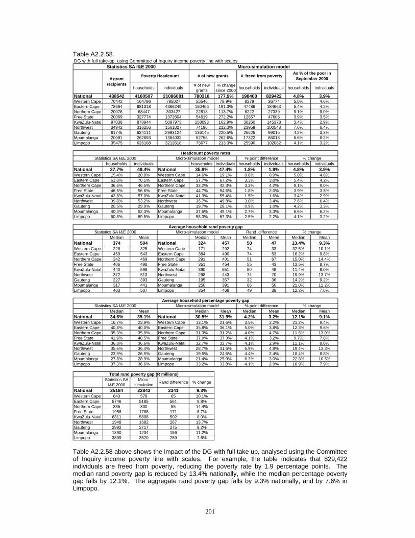
201
Table A2.2.58.
Table A2.2.58 above shows the impact of the DG with full take up, analysed using the Committee of Inquiry income poverty line with scales. For example, the table indicates that 829,422 individuals are freed from poverty, reducing the poverty rate by 1.9 percentage points. The median rand poverty gap is reduced by 13.4% nationally, while the median percentage poverty gap falls by 12.1%. The aggregate rand poverty gap falls by 9.3% nationally, and by 7.6% in Limpopo.
DG with full take-up, using Committee of Inquiry income poverty line with scales
households individuals # of new grants
% change since 2000 households individuals households individuals
National 438542 4160507 21086081 780318 177.9% 198400 829422 4.8% 3.9%Western Cape 70442 164796 795027 55546 78.9% 8279 36774 5.0% 4.6%Eastern Cape 78664 881318 4366249 150466 191.3% 47486 184663 5.4% 4.2%Northern Cape 20076 68447 303427 22818 113.7% 6222 27339 9.1% 9.0%Free State 20069 327774 1372604 54619 272.2% 12657 47605 3.9% 3.5%KwaZulu-Natal 97038 878944 5097973 158093 162.9% 30260 145378 3.4% 2.9%Northwest 34942 316256 1561027 74196 212.3% 23959 100548 7.6% 6.4%Gauteng 61745 634111 2993124 136145 220.5% 26625 99015 4.2% 3.3%Mpumalanga 20091 262693 1384032 52758 262.6% 17322 86018 6.6% 6.2%Limpopo 35475 626168 3212618 75677 213.3% 25590 102082 4.1% 3.2%
households individuals households individuals households individuals households individualsNational 37.7% 49.4% National 35.9% 47.4% 1.8% 1.9% 4.8% 3.9%Western Cape 15.4% 20.0% Western Cape 14.6% 19.1% 0.8% 0.9% 5.0% 4.6%Eastern Cape 61.0% 70.1% Eastern Cape 57.7% 67.2% 3.3% 3.0% 5.4% 4.2%Northern Cape 36.6% 46.5% Northern Cape 33.2% 42.3% 3.3% 4.2% 9.1% 9.0%Free State 46.5% 56.6% Free State 44.7% 54.6% 1.8% 2.0% 3.9% 3.5%KwaZulu-Natal 42.8% 57.0% KwaZulu-Natal 41.3% 55.4% 1.5% 1.6% 3.4% 2.9%Northwest 39.8% 53.2% Northwest 36.7% 49.8% 3.0% 3.4% 7.6% 6.4%Gauteng 20.5% 29.0% Gauteng 19.7% 28.1% 0.9% 1.0% 4.2% 3.3%Mpumalanga 40.3% 52.3% Mpumalanga 37.6% 49.1% 2.7% 3.3% 6.6% 6.2%Limpopo 60.8% 69.5% Limpopo 58.3% 67.3% 2.5% 2.2% 4.1% 3.2%
Median Mean Median Mean Median Mean Median MeanNational 374 504 National 324 457 50 47 13.4% 9.3%Western Cape 228 325 Western Cape 171 292 74 33 32.5% 10.1%Eastern Cape 459 543 Eastern Cape 384 490 74 53 16.2% 9.8%Northern Cape 342 469 Northern Cape 291 401 51 67 15.0% 14.4%Free State 406 498 Free State 351 454 55 43 13.5% 8.7%KwaZulu-Natal 440 598 KwaZulu-Natal 390 551 50 48 11.4% 8.0%Northwest 372 513 Northwest 298 443 74 70 19.9% 13.7%Gauteng 227 393 Gauteng 195 357 32 36 14.2% 9.2%Mpumalanga 317 441 Mpumalanga 250 391 66 50 21.0% 11.2%Limpopo 403 507 Limpopo 354 468 49 38 12.2% 7.6%
Median Mean Median Mean Median Mean Median MeanNational 34.6% 35.1% National 30.5% 31.9% 4.2% 3.2% 12.1% 9.1%Western Cape 16.7% 23.9% Western Cape 13.1% 21.6% 3.5% 2.2% 21.2% 9.4%Eastern Cape 40.8% 40.0% Eastern Cape 35.8% 36.1% 5.0% 3.8% 12.3% 9.6%Northern Cape 35.3% 35.9% Northern Cape 31.3% 31.2% 4.0% 4.7% 11.5% 13.0%Free State 41.9% 40.5% Free State 37.9% 37.3% 4.1% 3.2% 9.7% 7.8%KwaZulu-Natal 36.8% 36.6% KwaZulu-Natal 32.7% 33.7% 4.1% 2.9% 11.1% 8.0%Northwest 35.6% 36.4% Northwest 28.7% 31.6% 6.9% 4.8% 19.4% 13.3%Gauteng 23.9% 26.9% Gauteng 19.5% 24.6% 4.4% 2.4% 18.4% 8.8%Mpumalanga 27.8% 28.9% Mpumalanga 21.4% 25.9% 6.3% 3.0% 22.8% 10.5%Limpopo 37.3% 36.6% Limpopo 33.2% 33.8% 4.1% 2.9% 10.9% 7.9%
Statistics SA I&E 2000
Micro-simulation Rand difference % change
National 25184 22843 2341 9.3%Western Cape 643 578 65 10.1%Eastern Cape 5746 5185 561 9.8%Northern Cape 385 330 55 14.4%Free State 1958 1788 171 8.7%KwaZulu-Natal 6311 5808 502 8.0%Northwest 1948 1682 267 13.7%Gauteng 2992 2717 275 9.2%Mpumalanga 1390 1234 156 11.2%Limpopo 3809 3520 289 7.6%
Total rand poverty gap (R millions)
Statistics SA I&E 2000 Micro-simulation model
Micro-simulation modelStatistics SA I&E 2000
Poverty Headcount# grant
recipients
% point differenceAverage household percentage poverty gap
Average household rand poverty gap% change
% changeMicro-simulation model
% change
Headcount poverty rates
# of new grants # freed from poverty As % of the poor in September 2000
Statistics SA I&E 2000 % point difference
Statistics SA I&E 2000 Micro-simulation model Rand difference

202
Table A2.2.59.
Table A2.2.59 above shows the impact of the CSG at an annual level of R1200 in 2000, with full take up to the age 7, analysed using the Committee of Inquiry income poverty line with scales. For example, the table indicates that 893,766 individuals are freed from poverty, reducing the poverty rate by 2.1 percentage points. The median rand poverty gap is reduced by 15.8% nationally, while the median percentage poverty gap falls by 15.1%. The aggregate rand poverty gap falls by 13.3% nationally, and by 15.1% in Limpopo.
CSG to age 7 with full take-up, using Committee of Inquiry income poverty line with scales
households individuals # of new grants
% change since 2000 households individuals households individuals
National 463699 4160507 21086081 3296044 710.8% 173101 893766 4.2% 4.2%Western Cape 59407 164796 795027 116766 196.6% 14312 64814 8.7% 8.2%Eastern Cape 63038 881318 4366249 701101 1112.2% 25896 138630 2.9% 3.2%Northern Cape 19734 68447 303427 46674 236.5% 2710 13001 4.0% 4.3%Free State 18573 327774 1372604 179390 965.9% 7705 39392 2.4% 2.9%KwaZulu-Natal 70660 878944 5097973 880612 1246.3% 37826 200057 4.3% 3.9%Northwest 34341 316256 1561027 229190 667.4% 11613 59688 3.7% 3.8%Gauteng 107493 634111 2993124 383518 356.8% 32171 150614 5.1% 5.0%Mpumalanga 43704 262693 1384032 201777 461.7% 13296 73408 5.1% 5.3%Limpopo 46749 626168 3212618 557016 1191.5% 27572 154162 4.4% 4.8%
households individuals households individuals households individuals households individualsNational 37.7% 49.4% National 36.2% 47.3% 1.6% 2.1% 4.2% 4.2%Western Cape 15.4% 20.0% Western Cape 14.1% 18.4% 1.3% 1.6% 8.7% 8.2%Eastern Cape 61.0% 70.1% Eastern Cape 59.2% 67.9% 1.8% 2.2% 2.9% 3.2%Northern Cape 36.6% 46.5% Northern Cape 35.1% 44.5% 1.4% 2.0% 4.0% 4.3%Free State 46.5% 56.6% Free State 45.4% 55.0% 1.1% 1.6% 2.4% 2.9%KwaZulu-Natal 42.8% 57.0% KwaZulu-Natal 40.9% 54.8% 1.8% 2.2% 4.3% 3.9%Northwest 39.8% 53.2% Northwest 38.3% 51.2% 1.5% 2.0% 3.7% 3.8%Gauteng 20.5% 29.0% Gauteng 19.5% 27.6% 1.0% 1.5% 5.1% 5.0%Mpumalanga 40.3% 52.3% Mpumalanga 38.2% 49.6% 2.0% 2.8% 5.1% 5.3%Limpopo 60.8% 69.5% Limpopo 58.1% 66.2% 2.7% 3.3% 4.4% 4.8%
Median Mean Median Mean Median Mean Median MeanNational 374 504 National 315 437 59 67 15.8% 13.3%Western Cape 228 325 Western Cape 149 272 91 53 39.7% 16.2%Eastern Cape 459 543 Eastern Cape 368 472 91 72 19.8% 13.2%Northern Cape 342 469 Northern Cape 317 410 25 59 7.2% 12.6%Free State 406 498 Free State 360 449 46 49 11.4% 9.8%KwaZulu-Natal 440 598 KwaZulu-Natal 368 511 72 87 16.5% 14.6%Northwest 372 513 Northwest 318 454 54 59 14.6% 11.6%Gauteng 227 393 Gauteng 205 350 23 43 9.9% 10.9%Mpumalanga 317 441 Mpumalanga 267 379 50 62 15.7% 14.0%Limpopo 403 507 Limpopo 322 431 81 76 20.1% 15.1%
Median Mean Median Mean Median Mean Median MeanNational 34.6% 35.1% National 29.4% 30.8% 5.2% 4.3% 15.1% 12.4%Western Cape 16.7% 23.9% Western Cape 13.6% 20.1% 3.1% 3.8% 18.5% 15.7%Eastern Cape 40.8% 40.0% Eastern Cape 34.3% 35.1% 6.5% 4.9% 15.9% 12.3%Northern Cape 35.3% 35.9% Northern Cape 32.1% 31.7% 3.2% 4.2% 9.0% 11.6%Free State 41.9% 40.5% Free State 37.6% 36.8% 4.4% 3.7% 10.4% 9.1%KwaZulu-Natal 36.8% 36.6% KwaZulu-Natal 30.4% 31.5% 6.4% 5.1% 17.3% 13.8%Northwest 35.6% 36.4% Northwest 32.0% 32.7% 3.6% 3.7% 10.1% 10.2%Gauteng 23.9% 26.9% Gauteng 19.6% 24.1% 4.3% 2.9% 17.9% 10.6%Mpumalanga 27.8% 28.9% Mpumalanga 21.3% 25.0% 6.4% 3.9% 23.2% 13.4%Limpopo 37.3% 36.6% Limpopo 30.6% 31.5% 6.7% 5.1% 18.0% 13.9%
Statistics SA I&E 2000
Micro-simulation Rand difference % change
National 25184 21841 3343 13.3%Western Cape 643 539 104 16.2%Eastern Cape 5746 4988 758 13.2%Northern Cape 385 337 48 12.6%Free State 1958 1767 192 9.8%KwaZulu-Natal 6311 5389 921 14.6%Northwest 1948 1723 226 11.6%Gauteng 2992 2666 326 10.9%Mpumalanga 1390 1195 195 14.0%Limpopo 3809 3235 573 15.1%
Total rand poverty gap (R millions)
Statistics SA I&E 2000 Micro-simulation model
Micro-simulation modelStatistics SA I&E 2000
Poverty Headcount# grant
recipients
% point differenceAverage household percentage poverty gap
Average household rand poverty gap% change
% changeMicro-simulation model
% change
Headcount poverty rates
# of new grants # freed from poverty As % of the poor in September 2000
Statistics SA I&E 2000 % point difference
Statistics SA I&E 2000 Micro-simulation model Rand difference

203
Table A2.2.60.
Table A2.2.60 above shows the impact of the CSG at an annual level of R1200 in 2000, with full take up to the age 9, analysed using the Committee of Inquiry income poverty line with scales. For example, the table indicates that 1,268,179 individuals are freed from poverty, reducing the poverty rate by 3.0 percentage points. The median rand poverty gap is reduced by 22.4% nationally, while the median percentage poverty gap falls by 21.0%. The aggregate rand poverty gap falls by 17.7% nationally, and by 19.9% in Limpopo.
CSG to age 9 with full take-up, using Committee of Inquiry income poverty line with scales
households individuals # of new grants
% change since 2000 households individuals households individuals
National 463699 4160507 21086081 4438855 957.3% 240291 1268179 5.8% 6.0%Western Cape 59407 164796 795027 154864 260.7% 19619 95954 11.9% 12.1%Eastern Cape 63038 881318 4366249 954382 1514.0% 34128 176612 3.9% 4.0%Northern Cape 19734 68447 303427 58671 297.3% 3237 15984 4.7% 5.3%Free State 18573 327774 1372604 243808 1312.7% 11504 55961 3.5% 4.1%KwaZulu-Natal 70660 878944 5097973 1184537 1676.4% 52271 294848 5.9% 5.8%Northwest 34341 316256 1561027 305347 889.2% 14891 77611 4.7% 5.0%Gauteng 107493 634111 2993124 506783 471.5% 44794 225819 7.1% 7.5%Mpumalanga 43704 262693 1384032 280991 642.9% 19077 105802 7.3% 7.6%Limpopo 46749 626168 3212618 749472 1603.2% 40770 219588 6.5% 6.8%
households individuals households individuals households individuals households individualsNational 37.7% 49.4% National 35.6% 46.4% 2.2% 3.0% 5.8% 6.0%Western Cape 15.4% 20.0% Western Cape 13.6% 17.6% 1.8% 2.4% 11.9% 12.1%Eastern Cape 61.0% 70.1% Eastern Cape 58.7% 67.3% 2.4% 2.8% 3.9% 4.0%Northern Cape 36.6% 46.5% Northern Cape 34.8% 44.0% 1.7% 2.4% 4.7% 5.3%Free State 46.5% 56.6% Free State 44.9% 54.3% 1.6% 2.3% 3.5% 4.1%KwaZulu-Natal 42.8% 57.0% KwaZulu-Natal 40.2% 53.7% 2.5% 3.3% 5.9% 5.8%Northwest 39.8% 53.2% Northwest 37.9% 50.6% 1.9% 2.6% 4.7% 5.0%Gauteng 20.5% 29.0% Gauteng 19.1% 26.8% 1.4% 2.2% 7.1% 7.5%Mpumalanga 40.3% 52.3% Mpumalanga 37.4% 48.3% 2.9% 4.0% 7.3% 7.6%Limpopo 60.8% 69.5% Limpopo 56.8% 64.8% 4.0% 4.8% 6.5% 6.8%
Median Mean Median Mean Median Mean Median MeanNational 374 504 National 290 415 84 89 22.4% 17.7%Western Cape 228 325 Western Cape 134 258 111 67 48.5% 20.6%Eastern Cape 459 543 Eastern Cape 348 447 111 97 24.1% 17.8%Northern Cape 342 469 Northern Cape 298 396 44 73 12.8% 15.6%Free State 406 498 Free State 344 432 62 66 15.3% 13.2%KwaZulu-Natal 440 598 KwaZulu-Natal 336 482 105 116 23.8% 19.5%Northwest 372 513 Northwest 297 434 76 80 20.3% 15.5%Gauteng 227 393 Gauteng 185 337 42 56 18.6% 14.2%Mpumalanga 317 441 Mpumalanga 230 356 87 85 27.4% 19.2%Limpopo 403 507 Limpopo 296 406 107 101 26.6% 19.9%
Median Mean Median Mean Median Mean Median MeanNational 34.6% 35.1% National 27.4% 29.3% 7.3% 5.8% 21.0% 16.6%Western Cape 16.7% 23.9% Western Cape 12.0% 19.2% 4.7% 4.7% 28.3% 19.6%Eastern Cape 40.8% 40.0% Eastern Cape 32.7% 33.3% 8.1% 6.6% 19.8% 16.6%Northern Cape 35.3% 35.9% Northern Cape 28.8% 30.7% 6.5% 5.3% 18.5% 14.7%Free State 41.9% 40.5% Free State 36.0% 35.4% 6.0% 5.0% 14.2% 12.5%KwaZulu-Natal 36.8% 36.6% KwaZulu-Natal 28.2% 29.8% 8.6% 6.8% 23.4% 18.5%Northwest 35.6% 36.4% Northwest 30.1% 31.4% 5.5% 5.0% 15.4% 13.8%Gauteng 23.9% 26.9% Gauteng 18.3% 23.2% 5.6% 3.7% 23.5% 13.9%Mpumalanga 27.8% 28.9% Mpumalanga 19.3% 23.6% 8.4% 5.3% 30.4% 18.4%Limpopo 37.3% 36.6% Limpopo 28.0% 29.8% 9.2% 6.9% 24.8% 18.7%
Statistics SA I&E 2000
Micro-simulation Rand difference % change
National 25184 20730 4454 17.7%Western Cape 643 511 132 20.6%Eastern Cape 5746 4724 1022 17.8%Northern Cape 385 325 60 15.6%Free State 1958 1700 258 13.2%KwaZulu-Natal 6311 5083 1228 19.5%Northwest 1948 1646 302 15.5%Gauteng 2992 2566 426 14.2%Mpumalanga 1390 1123 267 19.2%Limpopo 3809 3050 759 19.9%
Total rand poverty gap (R millions)
Statistics SA I&E 2000 Micro-simulation model
Micro-simulation modelStatistics SA I&E 2000
Poverty Headcount# grant
recipients
% point differenceAverage household percentage poverty gap
Average household rand poverty gap% change
% changeMicro-simulation model
% change
Headcount poverty rates
# of new grants # freed from poverty As % of the poor in September 2000
Statistics SA I&E 2000 % point difference
Statistics SA I&E 2000 Micro-simulation model Rand difference

204
Table A2.2.61.
Table A2.2.61 above shows the impact of the CSG at an annual level of R1200 in 2000, with full take up to the age 11, analysed using the Committee of Inquiry income poverty line with scales. For example, the table indicates that 1,638,974 individuals are freed from poverty, reducing the poverty rate by 3.8 percentage points. The median rand poverty gap is reduced by 29.3% nationally, while the median percentage poverty gap falls by 27.2%. The aggregate rand poverty gap falls by 22.2% nationally, and by 25.0% in Limpopo.
CSG to age 11 with full take-up, using Committee of Inquiry income poverty line with scales
households individuals # of new grants
% change since 2000 households individuals households individuals
National 463699 4160507 21086081 5633296 1214.9% 310443 1638974 7.5% 7.8%Western Cape 59407 164796 795027 200063 336.8% 25144 119634 15.3% 15.0%Eastern Cape 63038 881318 4366249 1229486 1950.4% 46280 236409 5.3% 5.4%Northern Cape 19734 68447 303427 72679 368.3% 4151 21196 6.1% 7.0%Free State 18573 327774 1372604 310753 1673.1% 13635 65904 4.2% 4.8%KwaZulu-Natal 70660 878944 5097973 1476819 2090.0% 69018 387729 7.9% 7.6%Northwest 34341 316256 1561027 393537 1146.0% 19741 105469 6.2% 6.8%Gauteng 107493 634111 2993124 630503 586.6% 54598 283358 8.6% 9.5%Mpumalanga 43704 262693 1384032 360574 825.0% 24085 133280 9.2% 9.6%Limpopo 46749 626168 3212618 958882 2051.1% 53791 285995 8.6% 8.9%
households individuals households individuals households individuals households individualsNational 37.7% 49.4% National 34.9% 45.5% 2.8% 3.8% 7.5% 7.8%Western Cape 15.4% 20.0% Western Cape 13.1% 17.0% 2.4% 3.0% 15.3% 15.0%Eastern Cape 61.0% 70.1% Eastern Cape 57.8% 66.3% 3.2% 3.8% 5.3% 5.4%Northern Cape 36.6% 46.5% Northern Cape 34.4% 43.2% 2.2% 3.2% 6.1% 7.0%Free State 46.5% 56.6% Free State 44.6% 53.9% 1.9% 2.7% 4.2% 4.8%KwaZulu-Natal 42.8% 57.0% KwaZulu-Natal 39.4% 52.7% 3.4% 4.3% 7.9% 7.6%Northwest 39.8% 53.2% Northwest 37.3% 49.7% 2.5% 3.6% 6.2% 6.8%Gauteng 20.5% 29.0% Gauteng 18.8% 26.3% 1.8% 2.7% 8.6% 9.5%Mpumalanga 40.3% 52.3% Mpumalanga 36.6% 47.3% 3.7% 5.0% 9.2% 9.6%Limpopo 60.8% 69.5% Limpopo 55.5% 63.4% 5.2% 6.2% 8.6% 8.9%
Median Mean Median Mean Median Mean Median MeanNational 374 504 National 264 392 110 112 29.3% 22.2%Western Cape 228 325 Western Cape 111 239 131 86 57.4% 26.4%Eastern Cape 459 543 Eastern Cape 328 420 131 123 28.6% 22.7%Northern Cape 342 469 Northern Cape 280 379 62 90 18.1% 19.1%Free State 406 498 Free State 330 414 76 84 18.8% 16.9%KwaZulu-Natal 440 598 KwaZulu-Natal 309 455 131 144 29.7% 24.0%Northwest 372 513 Northwest 282 412 90 101 24.1% 19.7%Gauteng 227 393 Gauteng 175 324 53 69 23.2% 17.6%Mpumalanga 317 441 Mpumalanga 201 335 116 106 36.6% 24.1%Limpopo 403 507 Limpopo 268 380 135 127 33.4% 25.0%
Median Mean Median Mean Median Mean Median MeanNational 34.6% 35.1% National 25.2% 27.8% 9.4% 7.3% 27.2% 20.8%Western Cape 16.7% 23.9% Western Cape 10.1% 17.8% 6.6% 6.0% 39.7% 25.3%Eastern Cape 40.8% 40.0% Eastern Cape 29.9% 31.5% 10.9% 8.5% 26.8% 21.2%Northern Cape 35.3% 35.9% Northern Cape 27.1% 29.6% 8.2% 6.4% 23.2% 17.7%Free State 41.9% 40.5% Free State 34.4% 34.1% 7.5% 6.4% 17.9% 15.8%KwaZulu-Natal 36.8% 36.6% KwaZulu-Natal 26.4% 28.2% 10.4% 8.4% 28.2% 22.9%Northwest 35.6% 36.4% Northwest 27.9% 30.0% 7.6% 6.4% 21.5% 17.6%Gauteng 23.9% 26.9% Gauteng 16.7% 22.4% 7.2% 4.5% 30.0% 16.8%Mpumalanga 27.8% 28.9% Mpumalanga 18.5% 22.2% 9.3% 6.7% 33.4% 23.1%Limpopo 37.3% 36.6% Limpopo 25.5% 28.0% 11.7% 8.7% 31.5% 23.6%
Statistics SA I&E 2000
Micro-simulation Rand difference % change
National 25184 19588 5596 22.2%Western Cape 643 473 169 26.4%Eastern Cape 5746 4441 1306 22.7%Northern Cape 385 311 74 19.1%Free State 1958 1627 331 16.9%KwaZulu-Natal 6311 4794 1516 24.0%Northwest 1948 1565 384 19.7%Gauteng 2992 2465 527 17.6%Mpumalanga 1390 1055 335 24.1%Limpopo 3809 2855 954 25.0%
Total rand poverty gap (R millions)
Statistics SA I&E 2000 Micro-simulation model
Micro-simulation modelStatistics SA I&E 2000
Poverty Headcount# grant
recipients
% point differenceAverage household percentage poverty gap
Average household rand poverty gap% change
% changeMicro-simulation model
% change
Headcount poverty rates
# of new grants # freed from poverty As % of the poor in September 2000
Statistics SA I&E 2000 % point difference
Statistics SA I&E 2000 Micro-simulation model Rand difference

205
Table A2.2.62.
Table A2.2.62 above shows the impact of the CSG at an annual level of R1200 in 2000, with full take up to the age 14, analysed using the Committee of Inquiry income poverty line with scales. For example, the table indicates that 2,228,915 individuals are freed from poverty, reducing the poverty rate by 5.2 percentage points. The median rand poverty gap is reduced by 36.8% nationally, while the median percentage poverty gap falls by 35.5%. The aggregate rand poverty gap falls by 28.6% nationally, and by 32.4% in Limpopo.
CSG to age 14 with full take-up, using Committee of Inquiry income poverty line with scales
households individuals # of new grants
% change since 2000 households individuals households individuals
National 463699 4160507 21086081 7371762 1589.8% 423530 2228915 10.2% 10.6%Western Cape 59407 164796 795027 250588 421.8% 31317 158212 19.0% 19.9%Eastern Cape 63038 881318 4366249 1644685 2609.0% 76101 393864 8.6% 9.0%Northern Cape 19734 68447 303427 91709 464.7% 5312 26751 7.8% 8.8%Free State 18573 327774 1372604 408776 2200.9% 18765 85728 5.7% 6.2%KwaZulu-Natal 70660 878944 5097973 1907763 2699.9% 94879 527689 10.8% 10.4%Northwest 34341 316256 1561027 518808 1510.8% 23742 126518 7.5% 8.1%Gauteng 107493 634111 2993124 808298 752.0% 68100 352248 10.7% 11.8%Mpumalanga 43704 262693 1384032 477603 1092.8% 35332 190513 13.4% 13.8%Limpopo 46749 626168 3212618 1263532 2702.8% 69982 367392 11.2% 11.4%
households individuals households individuals households individuals households individualsNational 37.7% 49.4% National 33.9% 44.1% 3.8% 5.2% 10.2% 10.6%Western Cape 15.4% 20.0% Western Cape 12.5% 16.1% 2.9% 4.0% 19.0% 19.9%Eastern Cape 61.0% 70.1% Eastern Cape 55.8% 63.8% 5.3% 6.3% 8.6% 9.0%Northern Cape 36.6% 46.5% Northern Cape 33.7% 42.4% 2.8% 4.1% 7.8% 8.8%Free State 46.5% 56.6% Free State 43.9% 53.1% 2.7% 3.5% 5.7% 6.2%KwaZulu-Natal 42.8% 57.0% KwaZulu-Natal 38.2% 51.1% 4.6% 5.9% 10.8% 10.4%Northwest 39.8% 53.2% Northwest 36.8% 48.9% 3.0% 4.3% 7.5% 8.1%Gauteng 20.5% 29.0% Gauteng 18.3% 25.6% 2.2% 3.4% 10.7% 11.8%Mpumalanga 40.3% 52.3% Mpumalanga 34.9% 45.1% 5.4% 7.2% 13.4% 13.8%Limpopo 60.8% 69.5% Limpopo 54.0% 61.6% 6.8% 8.0% 11.2% 11.4%
Median Mean Median Mean Median Mean Median MeanNational 374 504 National 236 360 138 144 36.8% 28.6%Western Cape 228 325 Western Cape 72 223 179 102 78.5% 31.5%Eastern Cape 459 543 Eastern Cape 279 382 179 161 39.1% 29.7%Northern Cape 342 469 Northern Cape 261 357 81 112 23.7% 23.8%Free State 406 498 Free State 307 389 99 109 24.4% 21.9%KwaZulu-Natal 440 598 KwaZulu-Natal 273 415 167 183 38.0% 30.6%Northwest 372 513 Northwest 256 381 116 133 31.3% 25.8%Gauteng 227 393 Gauteng 150 305 77 89 33.9% 22.5%Mpumalanga 317 441 Mpumalanga 168 304 149 137 47.0% 31.0%Limpopo 403 507 Limpopo 225 343 178 164 44.2% 32.4%
Median Mean Median Mean Median Mean Median MeanNational 34.6% 35.1% National 22.3% 25.7% 12.3% 9.4% 35.5% 26.8%Western Cape 16.7% 23.9% Western Cape 7.4% 16.7% 9.3% 7.1% 55.6% 29.9%Eastern Cape 40.8% 40.0% Eastern Cape 26.2% 28.9% 14.6% 11.1% 35.7% 27.8%Northern Cape 35.3% 35.9% Northern Cape 26.6% 28.1% 8.7% 7.9% 24.5% 21.9%Free State 41.9% 40.5% Free State 31.6% 32.2% 10.3% 8.3% 24.7% 20.4%KwaZulu-Natal 36.8% 36.6% KwaZulu-Natal 23.9% 25.9% 12.8% 10.7% 34.9% 29.2%Northwest 35.6% 36.4% Northwest 25.3% 27.9% 10.3% 8.5% 28.8% 23.2%Gauteng 23.9% 26.9% Gauteng 14.4% 21.3% 9.5% 5.7% 39.7% 21.0%Mpumalanga 27.8% 28.9% Mpumalanga 15.3% 20.3% 12.4% 8.6% 44.8% 29.7%Limpopo 37.3% 36.6% Limpopo 21.6% 25.3% 15.6% 11.3% 42.0% 30.8%
Statistics SA I&E 2000
Micro-simulation Rand difference % change
National 25184 17982 7202 28.6%Western Cape 643 441 202 31.5%Eastern Cape 5746 4041 1705 29.7%Northern Cape 385 293 92 23.8%Free State 1958 1529 429 21.9%KwaZulu-Natal 6311 4381 1930 30.6%Northwest 1948 1445 503 25.8%Gauteng 2992 2318 674 22.5%Mpumalanga 1390 958 432 31.0%Limpopo 3809 2574 1235 32.4%
Total rand poverty gap (R millions)
Statistics SA I&E 2000 Micro-simulation model
Micro-simulation modelStatistics SA I&E 2000
Poverty Headcount# grant
recipients
% point differenceAverage household percentage poverty gap
Average household rand poverty gap% change
% changeMicro-simulation model
% change
Headcount poverty rates
# of new grants # freed from poverty As % of the poor in September 2000
Statistics SA I&E 2000 % point difference
Statistics SA I&E 2000 Micro-simulation model Rand difference

206
Table A2.2.63.
Table A2.2.63 above shows the impact of the CSG at an annual level of R1200 in 2000, with full take up to the age 16, analysed using the Committee of Inquiry income poverty line with scales. For example, the table indicates that 2,615,617 individuals are freed from poverty, reducing the poverty rate by 6.1 percentage points. The median rand poverty gap is reduced by 42.6% nationally, while the median percentage poverty gap falls by 41.3%. The aggregate rand poverty gap falls by 32.7% nationally, and by 36.7% in Limpopo.
CSG to age 16 with full take-up, using Committee of Inquiry income poverty line with scales
households individuals # of new grants
% change since 2000 households individuals households individuals
National 463699 4160507 21086081 8529103 1839.4% 496577 2615617 11.9% 12.4%Western Cape 59407 164796 795027 291943 491.4% 33870 177882 20.6% 22.4%Eastern Cape 63038 881318 4366249 1913147 3034.9% 94439 486918 10.7% 11.2%Northern Cape 19734 68447 303427 104713 530.6% 5912 30632 8.6% 10.1%Free State 18573 327774 1372604 479418 2581.3% 23735 104448 7.2% 7.6%KwaZulu-Natal 70660 878944 5097973 2200811 3114.6% 111210 618558 12.7% 12.1%Northwest 34341 316256 1561027 600583 1748.9% 28572 152802 9.0% 9.8%Gauteng 107493 634111 2993124 917098 853.2% 73181 384156 11.5% 12.8%Mpumalanga 43704 262693 1384032 556295 1272.9% 41868 221654 15.9% 16.0%Limpopo 46749 626168 3212618 1465095 3134.0% 83790 438567 13.4% 13.7%
households individuals households individuals households individuals households individualsNational 37.7% 49.4% National 33.2% 43.2% 4.5% 6.1% 11.9% 12.4%Western Cape 15.4% 20.0% Western Cape 12.2% 15.6% 3.2% 4.5% 20.6% 22.4%Eastern Cape 61.0% 70.1% Eastern Cape 54.5% 62.3% 6.5% 7.8% 10.7% 11.2%Northern Cape 36.6% 46.5% Northern Cape 33.4% 41.8% 3.2% 4.7% 8.6% 10.1%Free State 46.5% 56.6% Free State 43.2% 52.3% 3.4% 4.3% 7.2% 7.6%KwaZulu-Natal 42.8% 57.0% KwaZulu-Natal 37.4% 50.1% 5.4% 6.9% 12.7% 12.1%Northwest 39.8% 53.2% Northwest 36.2% 48.0% 3.6% 5.2% 9.0% 9.8%Gauteng 20.5% 29.0% Gauteng 18.2% 25.3% 2.4% 3.7% 11.5% 12.8%Mpumalanga 40.3% 52.3% Mpumalanga 33.9% 44.0% 6.4% 8.4% 15.9% 16.0%Limpopo 60.8% 69.5% Limpopo 52.6% 60.1% 8.1% 9.5% 13.4% 13.7%
Median Mean Median Mean Median Mean Median MeanNational 374 504 National 215 339 159 165 42.6% 32.7%Western Cape 228 325 Western Cape 57 208 204 117 89.4% 36.1%Eastern Cape 459 543 Eastern Cape 255 359 204 185 44.5% 34.0%Northern Cape 342 469 Northern Cape 242 343 100 126 29.1% 26.8%Free State 406 498 Free State 286 371 120 127 29.5% 25.5%KwaZulu-Natal 440 598 KwaZulu-Natal 244 389 197 209 44.7% 35.0%Northwest 372 513 Northwest 245 362 127 151 34.1% 29.5%Gauteng 227 393 Gauteng 140 292 87 101 38.5% 25.8%Mpumalanga 317 441 Mpumalanga 148 284 169 157 53.2% 35.7%Limpopo 403 507 Limpopo 199 321 204 186 50.5% 36.7%
Median Mean Median Mean Median Mean Median MeanNational 34.6% 35.1% National 20.3% 24.4% 14.3% 10.8% 41.3% 30.7%Western Cape 16.7% 23.9% Western Cape 5.9% 15.8% 10.8% 8.1% 64.8% 33.8%Eastern Cape 40.8% 40.0% Eastern Cape 24.0% 27.2% 16.9% 12.8% 41.3% 31.9%Northern Cape 35.3% 35.9% Northern Cape 25.7% 27.1% 9.6% 8.8% 27.2% 24.5%Free State 41.9% 40.5% Free State 30.1% 30.8% 11.8% 9.7% 28.2% 23.9%KwaZulu-Natal 36.8% 36.6% KwaZulu-Natal 21.5% 24.3% 15.3% 12.2% 41.5% 33.4%Northwest 35.6% 36.4% Northwest 22.6% 26.7% 13.0% 9.7% 36.5% 26.5%Gauteng 23.9% 26.9% Gauteng 13.9% 20.5% 10.0% 6.5% 41.9% 24.0%Mpumalanga 27.8% 28.9% Mpumalanga 14.0% 19.0% 13.7% 9.9% 49.4% 34.1%Limpopo 37.3% 36.6% Limpopo 18.9% 23.8% 18.4% 12.8% 49.4% 35.0%
Statistics SA I&E 2000
Micro-simulation Rand difference % change
National 25184 16946 8238 32.7%Western Cape 643 411 232 36.1%Eastern Cape 5746 3792 1954 34.0%Northern Cape 385 282 103 26.8%Free State 1958 1459 500 25.5%KwaZulu-Natal 6311 4102 2208 35.0%Northwest 1948 1374 574 29.5%Gauteng 2992 2221 771 25.8%Mpumalanga 1390 894 496 35.7%Limpopo 3809 2409 1400 36.7%
Total rand poverty gap (R millions)
Statistics SA I&E 2000 Micro-simulation model
Micro-simulation modelStatistics SA I&E 2000
Poverty Headcount# grant
recipients
% point differenceAverage household percentage poverty gap
Average household rand poverty gap% change
% changeMicro-simulation model
% change
Headcount poverty rates
# of new grants # freed from poverty As % of the poor in September 2000
Statistics SA I&E 2000 % point difference
Statistics SA I&E 2000 Micro-simulation model Rand difference

207
Table A2.2.64.
Table A2.2.64 above shows the impact of the CSG at an annual level of R1200 in 2000, with full take up to the age 18, analysed using the Committee of Inquiry income poverty line with scales. For example, the table indicates that 3,046,238 individuals are freed from poverty, reducing the poverty rate by 7.1 percentage points. The median rand poverty gap is reduced by 47.5% nationally, while the median percentage poverty gap falls by 45.9%. The aggregate rand poverty gap falls by 36.3% nationally, and by 40.5% in Limpopo.
CSG to age 18 with full take-up, using Committee of Inquiry income poverty line with scales
households individuals # of new grants
% change since 2000 households individuals households individuals
National 463699 4160507 21086081 9598463 2070.0% 584226 3046238 14.0% 14.4%Western Cape 59407 164796 795027 328707 553.3% 39138 205656 23.7% 25.9%Eastern Cape 63038 881318 4366249 2159087 3425.1% 111497 568498 12.7% 13.0%Northern Cape 19734 68447 303427 116464 590.2% 6188 31820 9.0% 10.5%Free State 18573 327774 1372604 553021 2977.6% 30011 128948 9.2% 9.4%KwaZulu-Natal 70660 878944 5097973 2462874 3485.5% 132973 734349 15.1% 14.4%Northwest 34341 316256 1561027 669557 1949.7% 34056 180584 10.8% 11.6%Gauteng 107493 634111 2993124 1030859 959.0% 80903 429855 12.8% 14.4%Mpumalanga 43704 262693 1384032 632102 1446.3% 50214 268433 19.1% 19.4%Limpopo 46749 626168 3212618 1645792 3520.5% 99246 498095 15.8% 15.5%
households individuals households individuals households individuals households individualsNational 37.7% 49.4% National 32.4% 42.2% 5.3% 7.1% 14.0% 14.4%Western Cape 15.4% 20.0% Western Cape 11.8% 14.9% 3.7% 5.2% 23.7% 25.9%Eastern Cape 61.0% 70.1% Eastern Cape 53.3% 61.0% 7.7% 9.1% 12.7% 13.0%Northern Cape 36.6% 46.5% Northern Cape 33.3% 41.6% 3.3% 4.9% 9.0% 10.5%Free State 46.5% 56.6% Free State 42.3% 51.3% 4.3% 5.3% 9.2% 9.4%KwaZulu-Natal 42.8% 57.0% KwaZulu-Natal 36.3% 48.8% 6.5% 8.2% 15.1% 14.4%Northwest 39.8% 53.2% Northwest 35.5% 47.1% 4.3% 6.2% 10.8% 11.6%Gauteng 20.5% 29.0% Gauteng 17.9% 24.8% 2.6% 4.2% 12.8% 14.4%Mpumalanga 40.3% 52.3% Mpumalanga 32.6% 42.2% 7.7% 10.2% 19.1% 19.4%Limpopo 60.8% 69.5% Limpopo 51.1% 58.8% 9.6% 10.8% 15.8% 15.5%
Median Mean Median Mean Median Mean Median MeanNational 374 504 National 196 321 178 183 47.5% 36.3%Western Cape 228 325 Western Cape 46 195 221 130 96.9% 40.1%Eastern Cape 459 543 Eastern Cape 238 338 221 205 48.2% 37.7%Northern Cape 342 469 Northern Cape 240 330 102 138 29.9% 29.5%Free State 406 498 Free State 272 352 134 146 32.9% 29.2%KwaZulu-Natal 440 598 KwaZulu-Natal 228 367 213 231 48.3% 38.7%Northwest 372 513 Northwest 237 347 136 167 36.4% 32.5%Gauteng 227 393 Gauteng 133 281 94 112 41.6% 28.5%Mpumalanga 317 441 Mpumalanga 130 264 187 177 59.1% 40.2%Limpopo 403 507 Limpopo 176 302 227 205 56.3% 40.5%
Median Mean Median Mean Median Mean Median MeanNational 34.6% 35.1% National 18.7% 23.2% 15.9% 12.0% 45.9% 34.0%Western Cape 16.7% 23.9% Western Cape 3.1% 14.9% 13.6% 8.9% 81.4% 37.3%Eastern Cape 40.8% 40.0% Eastern Cape 22.7% 25.8% 18.1% 14.2% 44.3% 35.5%Northern Cape 35.3% 35.9% Northern Cape 25.3% 26.2% 10.0% 9.8% 28.3% 27.2%Free State 41.9% 40.5% Free State 28.3% 29.3% 13.6% 11.2% 32.5% 27.7%KwaZulu-Natal 36.8% 36.6% KwaZulu-Natal 19.6% 23.1% 17.1% 13.5% 46.6% 36.9%Northwest 35.6% 36.4% Northwest 21.4% 25.8% 14.1% 10.6% 39.7% 29.2%Gauteng 23.9% 26.9% Gauteng 13.7% 19.9% 10.2% 7.1% 42.6% 26.2%Mpumalanga 27.8% 28.9% Mpumalanga 12.3% 17.8% 15.5% 11.1% 55.7% 38.4%Limpopo 37.3% 36.6% Limpopo 17.0% 22.5% 20.3% 14.1% 54.4% 38.5%
Statistics SA I&E 2000
Micro-simulation Rand difference % change
National 25184 16046 9139 36.3%Western Cape 643 385 258 40.1%Eastern Cape 5746 3578 2168 37.7%Northern Cape 385 271 114 29.5%Free State 1958 1386 572 29.2%KwaZulu-Natal 6311 3870 2440 38.7%Northwest 1948 1315 633 32.5%Gauteng 2992 2138 854 28.5%Mpumalanga 1390 831 559 40.2%Limpopo 3809 2268 1541 40.5%
Total rand poverty gap (R millions)
Statistics SA I&E 2000 Micro-simulation model
Micro-simulation modelStatistics SA I&E 2000
Poverty Headcount# grant
recipients
% point differenceAverage household percentage poverty gap
Average household rand poverty gap% change
% changeMicro-simulation model
% change
Headcount poverty rates
# of new grants # freed from poverty As % of the poor in September 2000
Statistics SA I&E 2000 % point difference
Statistics SA I&E 2000 Micro-simulation model Rand difference

208
Table A2.2.65.
Table A2.2.65 above shows the impact of the CSG at an annual level of R1606 in 2000, with full take up to the age 7, analysed using the Committee of Inquiry income poverty line with scales. For example, the table indicates that 1,205,020 individuals are freed from poverty, reducing the poverty rate by 2.8 percentage points. The median rand poverty gap is reduced by 22.6% nationally, while the median percentage poverty gap falls by 20.9%. The aggregate rand poverty gap falls by 17.4% nationally, and by 19.8% in Limpopo.
CSG(1606) to age 7 with full take-up, using Committee of Inquiry income poverty line with scales
households individuals # of new grants
% change since 2000 households individuals households individuals
National 463699 4160507 21086081 3296044 710.8% 231426 1205020 5.6% 5.7%Western Cape 59407 164796 795027 116766 196.6% 17646 82253 10.7% 10.3%Eastern Cape 63038 881318 4366249 701101 1112.2% 37008 194792 4.2% 4.5%Northern Cape 19734 68447 303427 46674 236.5% 3531 17396 5.2% 5.7%Free State 18573 327774 1372604 179390 965.9% 10820 51731 3.3% 3.8%KwaZulu-Natal 70660 878944 5097973 880612 1246.3% 51822 287495 5.9% 5.6%Northwest 34341 316256 1561027 229190 667.4% 13886 71150 4.4% 4.6%Gauteng 107493 634111 2993124 383518 356.8% 44134 209565 7.0% 7.0%Mpumalanga 43704 262693 1384032 201777 461.7% 19298 106763 7.3% 7.7%Limpopo 46749 626168 3212618 557016 1191.5% 33281 183875 5.3% 5.7%
households individuals households individuals households individuals households individualsNational 37.7% 49.4% National 35.6% 46.5% 2.1% 2.8% 5.6% 5.7%Western Cape 15.4% 20.0% Western Cape 13.8% 18.0% 1.7% 2.1% 10.7% 10.3%Eastern Cape 61.0% 70.1% Eastern Cape 58.5% 67.0% 2.6% 3.1% 4.2% 4.5%Northern Cape 36.6% 46.5% Northern Cape 34.7% 43.8% 1.9% 2.7% 5.2% 5.7%Free State 46.5% 56.6% Free State 45.0% 54.5% 1.5% 2.1% 3.3% 3.8%KwaZulu-Natal 42.8% 57.0% KwaZulu-Natal 40.3% 53.8% 2.5% 3.2% 5.9% 5.6%Northwest 39.8% 53.2% Northwest 38.0% 50.8% 1.7% 2.4% 4.4% 4.6%Gauteng 20.5% 29.0% Gauteng 19.1% 27.0% 1.4% 2.0% 7.0% 7.0%Mpumalanga 40.3% 52.3% Mpumalanga 37.3% 48.3% 3.0% 4.0% 7.3% 7.7%Limpopo 60.8% 69.5% Limpopo 57.5% 65.6% 3.2% 4.0% 5.3% 5.7%
Median Mean Median Mean Median Mean Median MeanNational 374 504 National 290 416 84 88 22.6% 17.4%Western Cape 228 325 Western Cape 125 258 114 67 50.1% 20.8%Eastern Cape 459 543 Eastern Cape 344 449 114 94 24.9% 17.4%Northern Cape 342 469 Northern Cape 298 392 44 77 12.8% 16.4%Free State 406 498 Free State 345 434 61 64 15.0% 12.9%KwaZulu-Natal 440 598 KwaZulu-Natal 336 483 104 115 23.7% 19.2%Northwest 372 513 Northwest 301 435 71 78 19.2% 15.3%Gauteng 227 393 Gauteng 177 337 50 56 22.2% 14.2%Mpumalanga 317 441 Mpumalanga 245 360 72 81 22.6% 18.3%Limpopo 403 507 Limpopo 298 406 104 100 25.9% 19.8%
Median Mean Median Mean Median Mean Median MeanNational 34.6% 35.1% National 27.4% 29.4% 7.2% 5.7% 20.9% 16.2%Western Cape 16.7% 23.9% Western Cape 12.0% 19.1% 4.7% 4.8% 28.3% 20.0%Eastern Cape 40.8% 40.0% Eastern Cape 32.3% 33.5% 8.6% 6.5% 21.0% 16.1%Northern Cape 35.3% 35.9% Northern Cape 28.8% 30.5% 6.5% 5.4% 18.5% 15.1%Free State 41.9% 40.5% Free State 36.2% 35.6% 5.7% 4.9% 13.6% 12.0%KwaZulu-Natal 36.8% 36.6% KwaZulu-Natal 28.6% 29.9% 8.2% 6.6% 22.3% 18.1%Northwest 35.6% 36.4% Northwest 30.5% 31.5% 5.1% 4.9% 14.4% 13.4%Gauteng 23.9% 26.9% Gauteng 18.8% 23.2% 5.1% 3.7% 21.4% 13.8%Mpumalanga 27.8% 28.9% Mpumalanga 20.0% 23.9% 7.8% 5.0% 28.0% 17.3%Limpopo 37.3% 36.6% Limpopo 28.3% 29.9% 9.0% 6.7% 24.0% 18.3%
Statistics SA I&E 2000
Micro-simulation Rand difference % change
National 25184 20792 4392 17.4%Western Cape 643 509 133 20.8%Eastern Cape 5746 4749 997 17.4%Northern Cape 385 322 63 16.4%Free State 1958 1706 253 12.9%KwaZulu-Natal 6311 5096 1215 19.2%Northwest 1948 1651 297 15.3%Gauteng 2992 2567 425 14.2%Mpumalanga 1390 1136 254 18.3%Limpopo 3809 3054 755 19.8%
% change
Headcount poverty rates
# of new grants # freed from poverty As % of the poor in September 2000
Statistics SA I&E 2000 % point difference
Statistics SA I&E 2000 Micro-simulation model Rand differenceAverage household rand poverty gap
% change
% changeMicro-simulation model
Total rand poverty gap (R millions)
Statistics SA I&E 2000 Micro-simulation model
Micro-simulation modelStatistics SA I&E 2000
Poverty Headcount# grant
recipients
% point differenceAverage household percentage poverty gap

209
Table A2.2.66.
Table A2.2.66 above shows the impact of the CSG at an annual level of R1606 in 2000, with full take up to the age 9, analysed using the Committee of Inquiry income poverty line with scales. For example, the table indicates that 1,766,530 individuals are freed from poverty, reducing the poverty rate by 4.1 percentage points. The median rand poverty gap is reduced by 29.8% nationally, while the median percentage poverty gap falls by 28.2%. The aggregate rand poverty gap falls by 23.1% nationally, and by 26.0% in Limpopo.
CSG(1606) to age 9 with full take-up, using Committee of Inquiry income poverty line with scales
households individuals # of new grants
% change since 2000 households individuals households individuals
National 463699 4160507 21086081 4438855 957.3% 331622 1766530 8.0% 8.4%Western Cape 59407 164796 795027 154864 260.7% 23340 113307 14.2% 14.3%Eastern Cape 63038 881318 4366249 954382 1514.0% 50801 271233 5.8% 6.2%Northern Cape 19734 68447 303427 58671 297.3% 4612 22821 6.7% 7.5%Free State 18573 327774 1372604 243808 1312.7% 15716 74594 4.8% 5.4%KwaZulu-Natal 70660 878944 5097973 1184537 1676.4% 72447 414604 8.2% 8.1%Northwest 34341 316256 1561027 305347 889.2% 19634 103731 6.2% 6.6%Gauteng 107493 634111 2993124 506783 471.5% 62091 316867 9.8% 10.6%Mpumalanga 43704 262693 1384032 280991 642.9% 27075 146812 10.3% 10.6%Limpopo 46749 626168 3212618 749472 1603.2% 55906 302561 8.9% 9.4%
households individuals households individuals households individuals households individualsNational 37.7% 49.4% National 34.7% 45.2% 3.0% 4.1% 8.0% 8.4%Western Cape 15.4% 20.0% Western Cape 13.2% 17.2% 2.2% 2.9% 14.2% 14.3%Eastern Cape 61.0% 70.1% Eastern Cape 57.5% 65.8% 3.5% 4.4% 5.8% 6.2%Northern Cape 36.6% 46.5% Northern Cape 34.1% 43.0% 2.5% 3.5% 6.7% 7.5%Free State 46.5% 56.6% Free State 44.3% 53.5% 2.2% 3.1% 4.8% 5.4%KwaZulu-Natal 42.8% 57.0% KwaZulu-Natal 39.2% 52.4% 3.5% 4.6% 8.2% 8.1%Northwest 39.8% 53.2% Northwest 37.3% 49.7% 2.5% 3.5% 6.2% 6.6%Gauteng 20.5% 29.0% Gauteng 18.5% 25.9% 2.0% 3.1% 9.8% 10.6%Mpumalanga 40.3% 52.3% Mpumalanga 36.1% 46.8% 4.2% 5.6% 10.3% 10.6%Limpopo 60.8% 69.5% Limpopo 55.3% 63.0% 5.4% 6.6% 8.9% 9.4%
Median Mean Median Mean Median Mean Median MeanNational 374 504 National 263 388 111 117 29.8% 23.1%Western Cape 228 325 Western Cape 111 240 140 85 61.3% 26.2%Eastern Cape 459 543 Eastern Cape 319 417 140 127 30.5% 23.3%Northern Cape 342 469 Northern Cape 272 374 70 95 20.6% 20.2%Free State 406 498 Free State 329 412 77 86 19.0% 17.3%KwaZulu-Natal 440 598 KwaZulu-Natal 308 446 133 153 30.1% 25.5%Northwest 372 513 Northwest 277 409 95 105 25.6% 20.4%Gauteng 227 393 Gauteng 168 320 59 73 26.1% 18.5%Mpumalanga 317 441 Mpumalanga 183 331 134 110 42.2% 25.0%Limpopo 403 507 Limpopo 265 375 138 132 34.3% 26.0%
Median Mean Median Mean Median Mean Median MeanNational 34.6% 35.1% National 24.9% 27.6% 9.8% 7.6% 28.2% 21.6%Western Cape 16.7% 23.9% Western Cape 10.6% 17.9% 6.1% 5.9% 36.3% 24.8%Eastern Cape 40.8% 40.0% Eastern Cape 29.6% 31.3% 11.3% 8.7% 27.6% 21.7%Northern Cape 35.3% 35.9% Northern Cape 26.8% 29.1% 8.5% 6.8% 24.2% 18.9%Free State 41.9% 40.5% Free State 34.1% 33.9% 7.9% 6.6% 18.7% 16.3%KwaZulu-Natal 36.8% 36.6% KwaZulu-Natal 25.9% 27.7% 10.9% 8.8% 29.6% 24.2%Northwest 35.6% 36.4% Northwest 27.6% 29.8% 7.9% 6.6% 22.3% 18.0%Gauteng 23.9% 26.9% Gauteng 16.5% 22.1% 7.4% 4.8% 30.8% 17.9%Mpumalanga 27.8% 28.9% Mpumalanga 17.3% 22.1% 10.4% 6.8% 37.5% 23.7%Limpopo 37.3% 36.6% Limpopo 25.7% 27.7% 11.6% 8.9% 31.2% 24.4%
Statistics SA I&E 2000
Micro-simulation Rand difference % change
National 25184 19360 5824 23.1%Western Cape 643 474 169 26.2%Eastern Cape 5746 4407 1339 23.3%Northern Cape 385 307 78 20.2%Free State 1958 1620 339 17.3%KwaZulu-Natal 6311 4700 1610 25.5%Northwest 1948 1552 397 20.4%Gauteng 2992 2438 554 18.5%Mpumalanga 1390 1043 347 25.0%Limpopo 3809 2817 992 26.0%
% change
Headcount poverty rates
# of new grants # freed from poverty As % of the poor in September 2000
Statistics SA I&E 2000 % point difference
Statistics SA I&E 2000 Micro-simulation model Rand differenceAverage household rand poverty gap
% change
% changeMicro-simulation model
Total rand poverty gap (R millions)
Statistics SA I&E 2000 Micro-simulation model
Micro-simulation modelStatistics SA I&E 2000
Poverty Headcount# grant
recipients
% point differenceAverage household percentage poverty gap

210
Table A2.2.67.
Table A2.2.67 above shows the impact of the CSG at an annual level of R1606 in 2000, with full take up to the age 11, analysed using the Committee of Inquiry income poverty line with scales. For example, the table indicates that 2,304,252 individuals are freed from poverty, reducing the poverty rate by 5.4 percentage points. The median rand poverty gap is reduced by 38.5% nationally, while the median percentage poverty gap falls by 36.4%. The aggregate rand poverty gap falls by 28.9% nationally, and by 32.6% in Limpopo.
CSG(1606) to age 11 with full take-up, using Committee of Inquiry income poverty line with scales
households individuals # of new grants
% change since 2000 households individuals households individuals
National 463699 4160507 21086081 5633296 1214.9% 430554 2304252 10.3% 10.9%Western Cape 59407 164796 795027 200063 336.8% 29440 143180 17.9% 18.0%Eastern Cape 63038 881318 4366249 1229486 1950.4% 71154 382789 8.1% 8.8%Northern Cape 19734 68447 303427 72679 368.3% 5553 28390 8.1% 9.4%Free State 18573 327774 1372604 310753 1673.1% 19321 90708 5.9% 6.6%KwaZulu-Natal 70660 878944 5097973 1476819 2090.0% 93921 534317 10.7% 10.5%Northwest 34341 316256 1561027 393537 1146.0% 27814 151422 8.8% 9.7%Gauteng 107493 634111 2993124 630503 586.6% 74540 384808 11.8% 12.9%Mpumalanga 43704 262693 1384032 360574 825.0% 36836 199112 14.0% 14.4%Limpopo 46749 626168 3212618 958882 2051.1% 71975 389526 11.5% 12.1%
households individuals households individuals households individuals households individualsNational 37.7% 49.4% National 33.8% 44.0% 3.9% 5.4% 10.3% 10.9%Western Cape 15.4% 20.0% Western Cape 12.7% 16.4% 2.8% 3.6% 17.9% 18.0%Eastern Cape 61.0% 70.1% Eastern Cape 56.1% 64.0% 4.9% 6.1% 8.1% 8.8%Northern Cape 36.6% 46.5% Northern Cape 33.6% 42.1% 3.0% 4.3% 8.1% 9.4%Free State 46.5% 56.6% Free State 43.8% 52.8% 2.7% 3.7% 5.9% 6.6%KwaZulu-Natal 42.8% 57.0% KwaZulu-Natal 38.2% 51.1% 4.6% 6.0% 10.7% 10.5%Northwest 39.8% 53.2% Northwest 36.3% 48.1% 3.5% 5.2% 8.8% 9.7%Gauteng 20.5% 29.0% Gauteng 18.1% 25.3% 2.4% 3.7% 11.8% 12.9%Mpumalanga 40.3% 52.3% Mpumalanga 34.6% 44.8% 5.6% 7.5% 14.0% 14.4%Limpopo 60.8% 69.5% Limpopo 53.8% 61.1% 7.0% 8.4% 11.5% 12.1%
Median Mean Median Mean Median Mean Median MeanNational 374 504 National 230 358 144 146 38.5% 28.9%Western Cape 228 325 Western Cape 60 216 184 109 80.6% 33.4%Eastern Cape 459 543 Eastern Cape 275 382 184 161 40.1% 29.7%Northern Cape 342 469 Northern Cape 255 353 87 116 25.4% 24.8%Free State 406 498 Free State 302 388 104 110 25.7% 22.1%KwaZulu-Natal 440 598 KwaZulu-Natal 264 411 176 188 39.9% 31.4%Northwest 372 513 Northwest 256 382 116 132 31.3% 25.6%Gauteng 227 393 Gauteng 145 304 82 90 36.1% 22.8%Mpumalanga 317 441 Mpumalanga 165 304 152 137 48.0% 31.1%Limpopo 403 507 Limpopo 225 342 177 165 44.0% 32.6%
Median Mean Median Mean Median Mean Median MeanNational 34.6% 35.1% National 22.0% 25.7% 12.6% 9.5% 36.4% 26.9%Western Cape 16.7% 23.9% Western Cape 6.8% 16.2% 9.9% 7.6% 59.5% 32.0%Eastern Cape 40.8% 40.0% Eastern Cape 25.8% 29.0% 15.0% 11.0% 36.8% 27.5%Northern Cape 35.3% 35.9% Northern Cape 25.4% 27.7% 9.9% 8.2% 28.0% 22.9%Free State 41.9% 40.5% Free State 31.4% 32.1% 10.5% 8.3% 25.0% 20.6%KwaZulu-Natal 36.8% 36.6% KwaZulu-Natal 23.6% 25.7% 13.2% 10.8% 35.8% 29.6%Northwest 35.6% 36.4% Northwest 24.9% 28.1% 10.7% 8.3% 30.1% 22.8%Gauteng 23.9% 26.9% Gauteng 14.3% 21.1% 9.6% 5.8% 40.2% 21.6%Mpumalanga 27.8% 28.9% Mpumalanga 15.1% 20.4% 12.7% 8.5% 45.8% 29.5%Limpopo 37.3% 36.6% Limpopo 21.3% 25.4% 15.9% 11.2% 42.7% 30.6%
Statistics SA I&E 2000
Micro-simulation Rand difference % change
National 25184 17900 7284 28.9%Western Cape 643 428 215 33.4%Eastern Cape 5746 4042 1704 29.7%Northern Cape 385 290 95 24.8%Free State 1958 1525 433 22.1%KwaZulu-Natal 6311 4330 1981 31.4%Northwest 1948 1449 499 25.6%Gauteng 2992 2310 682 22.8%Mpumalanga 1390 958 432 31.1%Limpopo 3809 2567 1242 32.6%
% change
Headcount poverty rates
# of new grants # freed from poverty As % of the poor in September 2000
Statistics SA I&E 2000 % point difference
Statistics SA I&E 2000 Micro-simulation model Rand differenceAverage household rand poverty gap
% change
% changeMicro-simulation model
Total rand poverty gap (R millions)
Statistics SA I&E 2000 Micro-simulation model
Micro-simulation modelStatistics SA I&E 2000
Poverty Headcount# grant
recipients
% point differenceAverage household percentage poverty gap

211
Table A2.2.68.
Table A2.2.68 above shows the impact of the CSG at an annual level of R1606 in 2000, with full take up to the age 14, analysed using the Committee of Inquiry income poverty line with scales. For example, the table indicates that 3,188,186 individuals are freed from poverty, reducing the poverty rate by 7.5 percentage points. The median rand poverty gap is reduced by 48.9% nationally, while the median percentage poverty gap falls by 47.3%. The aggregate rand poverty gap falls by 36.9% nationally, and by 41.6% in Limpopo.
CSG91606) to age 14 with full take-up, using Committee of Inquiry income poverty line with scales
households individuals # of new grants
% change since 2000 households individuals households individuals
National 463699 4160507 21086081 7371762 1589.8% 588174 3188186 14.1% 15.1%Western Cape 59407 164796 795027 250588 421.8% 38648 206291 23.5% 25.9%Eastern Cape 63038 881318 4366249 1644685 2609.0% 105568 565388 12.0% 12.9%Northern Cape 19734 68447 303427 91709 464.7% 7134 36965 10.4% 12.2%Free State 18573 327774 1372604 408776 2200.9% 26514 122091 8.1% 8.9%KwaZulu-Natal 70660 878944 5097973 1907763 2699.9% 130257 765702 14.8% 15.0%Northwest 34341 316256 1561027 518808 1510.8% 36465 199750 11.5% 12.8%Gauteng 107493 634111 2993124 808298 752.0% 89327 464186 14.1% 15.5%Mpumalanga 43704 262693 1384032 477603 1092.8% 52241 284607 19.9% 20.6%Limpopo 46749 626168 3212618 1263532 2702.8% 102020 543206 16.3% 16.9%
households individuals households individuals households individuals households individualsNational 37.7% 49.4% National 32.4% 41.9% 5.3% 7.5% 14.1% 15.1%Western Cape 15.4% 20.0% Western Cape 11.8% 14.8% 3.6% 5.2% 23.5% 25.9%Eastern Cape 61.0% 70.1% Eastern Cape 53.7% 61.0% 7.3% 9.1% 12.0% 12.9%Northern Cape 36.6% 46.5% Northern Cape 32.8% 40.8% 3.8% 5.7% 10.4% 12.2%Free State 46.5% 56.6% Free State 42.8% 51.6% 3.8% 5.0% 8.1% 8.9%KwaZulu-Natal 42.8% 57.0% KwaZulu-Natal 36.4% 48.5% 6.3% 8.6% 14.8% 15.0%Northwest 39.8% 53.2% Northwest 35.2% 46.4% 4.6% 6.8% 11.5% 12.8%Gauteng 20.5% 29.0% Gauteng 17.6% 24.5% 2.9% 4.5% 14.1% 15.5%Mpumalanga 40.3% 52.3% Mpumalanga 32.3% 41.6% 8.0% 10.8% 19.9% 20.6%Limpopo 60.8% 69.5% Limpopo 50.9% 57.8% 9.9% 11.8% 16.3% 16.9%
Median Mean Median Mean Median Mean Median MeanNational 374 504 National 191 318 183 186 48.9% 36.9%Western Cape 228 325 Western Cape 40 197 239 128 104.6% 39.4%Eastern Cape 459 543 Eastern Cape 220 335 239 208 52.0% 38.4%Northern Cape 342 469 Northern Cape 230 325 112 144 32.8% 30.6%Free State 406 498 Free State 274 356 132 142 32.5% 28.6%KwaZulu-Natal 440 598 KwaZulu-Natal 217 361 224 237 50.8% 39.6%Northwest 372 513 Northwest 230 343 143 171 38.3% 33.3%Gauteng 227 393 Gauteng 118 279 109 114 48.1% 29.0%Mpumalanga 317 441 Mpumalanga 130 266 187 175 59.1% 39.7%Limpopo 403 507 Limpopo 176 296 227 211 56.3% 41.6%
Median Mean Median Mean Median Mean Median MeanNational 34.6% 35.1% National 18.3% 23.1% 16.4% 12.1% 47.3% 34.3%Western Cape 16.7% 23.9% Western Cape 3.8% 15.0% 12.9% 8.9% 77.1% 37.2%Eastern Cape 40.8% 40.0% Eastern Cape 21.7% 25.7% 19.1% 14.3% 46.9% 35.7%Northern Cape 35.3% 35.9% Northern Cape 23.1% 25.8% 12.2% 10.1% 34.5% 28.1%Free State 41.9% 40.5% Free State 27.8% 29.7% 14.1% 10.7% 33.6% 26.5%KwaZulu-Natal 36.8% 36.6% KwaZulu-Natal 18.7% 22.9% 18.1% 13.7% 49.2% 37.5%Northwest 35.6% 36.4% Northwest 21.2% 25.6% 14.3% 10.8% 40.3% 29.8%Gauteng 23.9% 26.9% Gauteng 12.3% 19.7% 11.6% 7.2% 48.4% 26.8%Mpumalanga 27.8% 28.9% Mpumalanga 11.9% 18.0% 15.9% 10.8% 57.3% 37.5%Limpopo 37.3% 36.6% Limpopo 16.9% 22.2% 20.4% 14.4% 54.7% 39.4%
Statistics SA I&E 2000
Micro-simulation Rand difference % change
National 25184 15897 9287 36.9%Western Cape 643 390 253 39.4%Eastern Cape 5746 3542 2204 38.4%Northern Cape 385 267 118 30.6%Free State 1958 1399 560 28.6%KwaZulu-Natal 6311 3811 2499 39.6%Northwest 1948 1301 648 33.3%Gauteng 2992 2124 868 29.0%Mpumalanga 1390 839 551 39.7%Limpopo 3809 2223 1586 41.6%
% change
Headcount poverty rates
# of new grants # freed from poverty As % of the poor in September 2000
Statistics SA I&E 2000 % point difference
Statistics SA I&E 2000 Micro-simulation model Rand differenceAverage household rand poverty gap
% change
% changeMicro-simulation model
Total rand poverty gap (R millions)
Statistics SA I&E 2000 Micro-simulation model
Micro-simulation modelStatistics SA I&E 2000
Poverty Headcount# grant
recipients
% point differenceAverage household percentage poverty gap

212
Table A2.2.69.
Table A2.2.69 above shows the impact of the CSG at an annual level of R1606 in 2000, with full take up to the age 16, analysed using the Committee of Inquiry income poverty line with scales. For example, the table indicates that 3,815,797 individuals are freed from poverty, reducing the poverty rate by 8.9 percentage points. The median rand poverty gap is reduced by 56.4% nationally, while the median percentage poverty gap falls by 55.8%. The aggregate rand poverty gap falls by 41.9% nationally, and by 46.8% in Limpopo.
CSG(1606) to age16 with full take-up, using Committee of Inquiry income poverty line with scales
households individuals # of new grants
% change since 2000 households individuals households individuals
National 463699 4160507 21086081 8529103 1839.4% 703715 3815797 16.9% 18.1%Western Cape 59407 164796 795027 291943 491.4% 40963 221745 24.9% 27.9%Eastern Cape 63038 881318 4366249 1913147 3034.9% 137150 726461 15.6% 16.6%Northern Cape 19734 68447 303427 104713 530.6% 7642 39269 11.2% 12.9%Free State 18573 327774 1372604 479418 2581.3% 35587 160007 10.9% 11.7%KwaZulu-Natal 70660 878944 5097973 2200811 3114.6% 152246 891317 17.3% 17.5%Northwest 34341 316256 1561027 600583 1748.9% 44247 246359 14.0% 15.8%Gauteng 107493 634111 2993124 917098 853.2% 101265 548621 16.0% 18.3%Mpumalanga 43704 262693 1384032 556295 1272.9% 63476 349681 24.2% 25.3%Limpopo 46749 626168 3212618 1465095 3134.0% 121139 632337 19.3% 19.7%
households individuals households individuals households individuals households individualsNational 37.7% 49.4% National 31.3% 40.4% 6.4% 8.9% 16.9% 18.1%Western Cape 15.4% 20.0% Western Cape 11.6% 14.4% 3.8% 5.6% 24.9% 27.9%Eastern Cape 61.0% 70.1% Eastern Cape 51.5% 58.5% 9.5% 11.7% 15.6% 16.6%Northern Cape 36.6% 46.5% Northern Cape 32.5% 40.5% 4.1% 6.0% 11.2% 12.9%Free State 46.5% 56.6% Free State 41.5% 50.0% 5.1% 6.6% 10.9% 11.7%KwaZulu-Natal 42.8% 57.0% KwaZulu-Natal 35.4% 47.1% 7.4% 10.0% 17.3% 17.5%Northwest 39.8% 53.2% Northwest 34.2% 44.8% 5.6% 8.4% 14.0% 15.8%Gauteng 20.5% 29.0% Gauteng 17.2% 23.7% 3.3% 5.3% 16.0% 18.3%Mpumalanga 40.3% 52.3% Mpumalanga 30.5% 39.1% 9.7% 13.2% 24.2% 25.3%Limpopo 60.8% 69.5% Limpopo 49.0% 55.9% 11.8% 13.7% 19.3% 19.7%
Median Mean Median Mean Median Mean Median MeanNational 374 504 National 163 293 211 211 56.4% 41.9%Western Cape 228 325 Western Cape 13 179 265 146 116.3% 44.9%Eastern Cape 459 543 Eastern Cape 193 306 265 237 57.9% 43.6%Northern Cape 342 469 Northern Cape 207 308 135 161 39.6% 34.4%Free State 406 498 Free State 249 333 158 165 38.8% 33.1%KwaZulu-Natal 440 598 KwaZulu-Natal 173 329 268 270 60.8% 45.1%Northwest 372 513 Northwest 203 320 169 194 45.5% 37.7%Gauteng 227 393 Gauteng 104 263 123 130 54.2% 33.1%Mpumalanga 317 441 Mpumalanga 106 242 210 199 66.4% 45.2%Limpopo 403 507 Limpopo 139 270 264 237 65.6% 46.8%
Median Mean Median Mean Median Mean Median MeanNational 34.6% 35.1% National 15.3% 21.4% 19.3% 13.7% 55.8% 39.1%Western Cape 16.7% 23.9% Western Cape 1.1% 13.9% 15.6% 10.0% 93.6% 41.8%Eastern Cape 40.8% 40.0% Eastern Cape 18.7% 23.7% 22.1% 16.3% 54.2% 40.7%Northern Cape 35.3% 35.9% Northern Cape 21.6% 24.7% 13.7% 11.3% 38.9% 31.4%Free State 41.9% 40.5% Free State 25.7% 28.0% 16.2% 12.5% 38.7% 30.9%KwaZulu-Natal 36.8% 36.6% KwaZulu-Natal 15.7% 21.0% 21.1% 15.6% 57.3% 42.7%Northwest 35.6% 36.4% Northwest 18.7% 24.1% 16.9% 12.3% 47.5% 33.8%Gauteng 23.9% 26.9% Gauteng 11.2% 18.7% 12.7% 8.2% 53.2% 30.6%Mpumalanga 27.8% 28.9% Mpumalanga 9.0% 16.5% 18.8% 12.4% 67.7% 42.8%Limpopo 37.3% 36.6% Limpopo 13.0% 20.4% 24.3% 16.2% 65.2% 44.2%
Statistics SA I&E 2000
Micro-simulation Rand difference % change
National 25184 14629 10556 41.9%Western Cape 643 354 289 44.9%Eastern Cape 5746 3238 2508 43.6%Northern Cape 385 253 132 34.4%Free State 1958 1310 648 33.1%KwaZulu-Natal 6311 3467 2844 45.1%Northwest 1948 1214 734 37.7%Gauteng 2992 2002 990 33.1%Mpumalanga 1390 762 628 45.2%Limpopo 3809 2026 1782 46.8%
% change
Headcount poverty rates
# of new grants # freed from poverty As % of the poor in September 2000
Statistics SA I&E 2000 % point difference
Statistics SA I&E 2000 Micro-simulation model Rand differenceAverage household rand poverty gap
% change
% changeMicro-simulation model
Total rand poverty gap (R millions)
Statistics SA I&E 2000 Micro-simulation model
Micro-simulation modelStatistics SA I&E 2000
Poverty Headcount# grant
recipients
% point differenceAverage household percentage poverty gap

213
Table A2.2.70.
Table A2.2.70 above shows the impact of the CSG at an annual level of R1606 in 2000, with full take up to the age 18, analysed using the Committee of Inquiry income poverty line with scales. For example, the table indicates that 4,425,587 individuals are freed from poverty, reducing the poverty rate by 10.4 percentage points. The median rand poverty gap is reduced by 62.4% nationally, while the median percentage poverty gap falls by 61.1%. The aggregate rand poverty gap falls by 46.2% nationally, and by 51.0% in Limpopo.
CSG(1606) to age 18 with full take-up, using Committee of Inquiry income poverty line with scales
households individuals # of new grants
% change since 2000 households individuals households individuals
National 463699 4160507 21086081 9598463 2070.0% 823312 4425587 19.8% 21.0%Western Cape 59407 164796 795027 328707 553.3% 46371 249053 28.1% 31.3%Eastern Cape 63038 881318 4366249 2159087 3425.1% 163548 854930 18.6% 19.6%Northern Cape 19734 68447 303427 116464 590.2% 8099 41718 11.8% 13.7%Free State 18573 327774 1372604 553021 2977.6% 43848 194208 13.4% 14.1%KwaZulu-Natal 70660 878944 5097973 2462874 3485.5% 178906 1041747 20.4% 20.4%Northwest 34341 316256 1561027 669557 1949.7% 51753 285988 16.4% 18.3%Gauteng 107493 634111 2993124 1030859 959.0% 112351 599753 17.7% 20.0%Mpumalanga 43704 262693 1384032 632102 1446.3% 71224 393398 27.1% 28.4%Limpopo 46749 626168 3212618 1645792 3520.5% 147212 764792 23.5% 23.8%
households individuals households individuals households individuals households individualsNational 37.7% 49.4% National 30.3% 39.0% 7.5% 10.4% 19.8% 21.0%Western Cape 15.4% 20.0% Western Cape 11.1% 13.8% 4.3% 6.3% 28.1% 31.3%Eastern Cape 61.0% 70.1% Eastern Cape 49.7% 56.4% 11.3% 13.7% 18.6% 19.6%Northern Cape 36.6% 46.5% Northern Cape 32.2% 40.1% 4.3% 6.4% 11.8% 13.7%Free State 46.5% 56.6% Free State 40.3% 48.6% 6.2% 8.0% 13.4% 14.1%KwaZulu-Natal 42.8% 57.0% KwaZulu-Natal 34.1% 45.4% 8.7% 11.7% 20.4% 20.4%Northwest 39.8% 53.2% Northwest 33.2% 43.5% 6.5% 9.8% 16.4% 18.3%Gauteng 20.5% 29.0% Gauteng 16.9% 23.2% 3.6% 5.8% 17.7% 20.0%Mpumalanga 40.3% 52.3% Mpumalanga 29.4% 37.5% 10.9% 14.9% 27.1% 28.4%Limpopo 60.8% 69.5% Limpopo 46.5% 53.0% 14.3% 16.6% 23.5% 23.8%
Median Mean Median Mean Median Mean Median MeanNational 374 504 National 141 271 234 233 62.4% 46.2%Western Cape 228 325 Western Cape 0 164 290 162 127.0% 49.7%Eastern Cape 459 543 Eastern Cape 169 282 290 262 63.2% 48.1%Northern Cape 342 469 Northern Cape 194 291 148 178 43.2% 37.9%Free State 406 498 Free State 224 309 182 188 44.8% 37.8%KwaZulu-Natal 440 598 KwaZulu-Natal 150 302 290 296 65.9% 49.5%Northwest 372 513 Northwest 172 300 200 213 53.8% 41.5%Gauteng 227 393 Gauteng 99 250 128 143 56.4% 36.4%Mpumalanga 317 441 Mpumalanga 80 218 237 223 74.9% 50.6%Limpopo 403 507 Limpopo 118 248 285 259 70.8% 51.0%
Median Mean Median Mean Median Mean Median MeanNational 34.6% 35.1% National 13.5% 20.0% 21.2% 15.1% 61.1% 43.0%Western Cape 16.7% 23.9% Western Cape 0.0% 12.9% 16.7% 11.0% 100.0% 45.9%Eastern Cape 40.8% 40.0% Eastern Cape 16.9% 22.0% 24.0% 18.0% 58.7% 45.0%Northern Cape 35.3% 35.9% Northern Cape 21.1% 23.4% 14.2% 12.5% 40.3% 34.8%Free State 41.9% 40.5% Free State 23.3% 26.0% 18.6% 14.4% 44.4% 35.7%KwaZulu-Natal 36.8% 36.6% KwaZulu-Natal 13.8% 19.5% 22.9% 17.1% 62.3% 46.7%Northwest 35.6% 36.4% Northwest 16.2% 22.9% 19.3% 13.5% 54.4% 37.2%Gauteng 23.9% 26.9% Gauteng 10.1% 18.0% 13.8% 9.0% 57.6% 33.3%Mpumalanga 27.8% 28.9% Mpumalanga 6.4% 15.0% 21.3% 13.8% 76.8% 47.9%Limpopo 37.3% 36.6% Limpopo 11.0% 19.0% 26.3% 17.7% 70.6% 48.2%
Statistics SA I&E 2000
Micro-simulation Rand difference % change
National 25184 13544 11641 46.2%Western Cape 643 323 319 49.7%Eastern Cape 5746 2979 2767 48.1%Northern Cape 385 239 146 37.9%Free State 1958 1217 741 37.8%KwaZulu-Natal 6311 3190 3121 49.5%Northwest 1948 1140 809 41.5%Gauteng 2992 1901 1091 36.4%Mpumalanga 1390 686 704 50.6%Limpopo 3809 1865 1944 51.0%
% change
Headcount poverty rates
# of new grants # freed from poverty As % of the poor in September 2000
Statistics SA I&E 2000 % point difference
Statistics SA I&E 2000 Micro-simulation model Rand differenceAverage household rand poverty gap
% change
% changeMicro-simulation model
Total rand poverty gap (R millions)
Statistics SA I&E 2000 Micro-simulation model
Micro-simulation modelStatistics SA I&E 2000
Poverty Headcount# grant
recipients
% point differenceAverage household percentage poverty gap

214
Table A2.2.71.
Table A2.2.71 above shows the impact of all grants with full take up, with the CSG at an annual level of R1200 in 2000, analysed using the Committee of Inquiry income poverty line with scales. For example, the table indicates that 3,842,326 individuals are freed from poverty, reducing the poverty rate by 9.0 percentage points. The median rand poverty gap is reduced by 56.9% nationally, while the median percentage poverty gap falls by 54.8%. The aggregate rand poverty gap falls by 39.9% nationally, and by 41.4% in Limpopo.
All grants with full take-up, using Committee of Inquiry income poverty line with scales
households individuals # of new grants
% change since 2000 households individuals households individuals
National 2656508 4160507 21086081 8545415 321.7% 767198 3842326 18.4% 18.2%Western Cape 241897 164796 795027 334220 138.2% 45263 217866 27.5% 27.4%Eastern Cape 499290 881318 4366249 1870227 374.6% 161379 766792 18.3% 17.6%Northern Cape 69402 68447 303427 120919 174.2% 14057 66809 20.5% 22.0%Free State 131645 327774 1372604 484791 368.3% 43204 198249 13.2% 14.4%KwaZulu-Natal 522017 878944 5097973 2147562 411.4% 157122 848697 17.9% 16.6%Northwest 208084 316256 1561027 619848 297.9% 58887 291580 18.6% 18.7%Gauteng 471943 634111 2993124 1048047 222.1% 116827 582179 18.4% 19.5%Mpumalanga 161387 262693 1384032 542950 336.4% 57818 309164 22.0% 22.3%Limpopo 350843 626168 3212618 1376851 392.4% 112641 560990 18.0% 17.5%
households individuals households individuals households individuals households individualsNational 37.7% 49.4% National 30.8% 40.4% 7.0% 9.0% 18.4% 18.2%Western Cape 15.4% 20.0% Western Cape 11.2% 14.5% 4.2% 5.5% 27.5% 27.4%Eastern Cape 61.0% 70.1% Eastern Cape 49.9% 57.8% 11.2% 12.3% 18.3% 17.6%Northern Cape 36.6% 46.5% Northern Cape 29.1% 36.2% 7.5% 10.2% 20.5% 22.0%Free State 46.5% 56.6% Free State 40.4% 48.4% 6.1% 8.2% 13.2% 14.4%KwaZulu-Natal 42.8% 57.0% KwaZulu-Natal 35.1% 47.5% 7.6% 9.5% 17.9% 16.6%Northwest 39.8% 53.2% Northwest 32.3% 43.3% 7.4% 9.9% 18.6% 18.7%Gauteng 20.5% 29.0% Gauteng 16.7% 23.4% 3.8% 5.6% 18.4% 19.5%Mpumalanga 40.3% 52.3% Mpumalanga 31.4% 40.6% 8.9% 11.7% 22.0% 22.3%Limpopo 60.8% 69.5% Limpopo 49.8% 57.4% 10.9% 12.1% 18.0% 17.5%
Median Mean Median Mean Median Mean Median MeanNational 374 504 National 161 303 213 201 56.9% 39.9%Western Cape 228 325 Western Cape 24 193 265 132 116.3% 40.5%Eastern Cape 459 543 Eastern Cape 193 316 265 227 57.8% 41.8%Northern Cape 342 469 Northern Cape 174 291 168 178 49.2% 37.9%Free State 406 498 Free State 249 336 158 162 38.8% 32.5%KwaZulu-Natal 440 598 KwaZulu-Natal 190 352 250 246 56.8% 41.1%Northwest 372 513 Northwest 152 304 220 209 59.1% 40.7%Gauteng 227 393 Gauteng 90 254 137 139 60.4% 35.4%Mpumalanga 317 441 Mpumalanga 110 257 207 184 65.3% 41.6%Limpopo 403 507 Limpopo 163 297 239 210 59.4% 41.4%
Median Mean Median Mean Median Mean Median MeanNational 34.6% 35.1% National 15.7% 21.8% 19.0% 13.3% 54.8% 37.9%Western Cape 16.7% 23.9% Western Cape 2.0% 14.3% 14.7% 9.6% 88.3% 40.1%Eastern Cape 40.8% 40.0% Eastern Cape 19.7% 24.0% 21.1% 16.0% 51.8% 39.9%Northern Cape 35.3% 35.9% Northern Cape 20.9% 23.3% 14.4% 12.6% 40.7% 35.1%Free State 41.9% 40.5% Free State 26.9% 28.4% 15.1% 12.1% 35.9% 29.9%KwaZulu-Natal 36.8% 36.6% KwaZulu-Natal 17.4% 22.0% 19.3% 14.6% 52.5% 39.9%Northwest 35.6% 36.4% Northwest 15.6% 22.6% 20.0% 13.8% 56.1% 37.8%Gauteng 23.9% 26.9% Gauteng 8.8% 18.2% 15.1% 8.7% 63.2% 32.4%Mpumalanga 27.8% 28.9% Mpumalanga 9.8% 17.5% 17.9% 11.4% 64.5% 39.5%Limpopo 37.3% 36.6% Limpopo 15.6% 22.0% 21.6% 14.6% 58.0% 39.9%
Statistics SA I&E 2000
Micro-simulation Rand difference % change
National 25184 15136 10048 39.9%Western Cape 643 382 261 40.5%Eastern Cape 5746 3342 2404 41.8%Northern Cape 385 239 146 37.9%Free State 1958 1321 637 32.5%KwaZulu-Natal 6311 3718 2593 41.1%Northwest 1948 1155 794 40.7%Gauteng 2992 1934 1058 35.4%Mpumalanga 1390 811 579 41.6%Limpopo 3809 2231 1577 41.4%
% change
Headcount poverty rates
# of new grants # freed from poverty As % of the poor in September 2000
Statistics SA I&E 2000 % point difference
Statistics SA I&E 2000 Micro-simulation model Rand differenceAverage household rand poverty gap
% change
% changeMicro-simulation model
Total rand poverty gap (R millions)
Statistics SA I&E 2000 Micro-simulation model
Micro-simulation modelStatistics SA I&E 2000
Poverty Headcount# grant
recipients
% point differenceAverage household percentage poverty gap

215
Table A2.2.72.
Table A2.2.54 above shows the impact of all grants with full take up, with the CSG at an annual level of R1606 in 2000, analysed using the Committee of Inquiry income poverty line with scales. For example, the table indicates that 4,861,052 individuals are freed from poverty, reducing the poverty rate by 11.4 percentage points. The median rand poverty gap is reduced by 68.1% nationally, while the median percentage poverty gap falls by 66.2%. The aggregate rand poverty gap falls by 47.4% nationally, and by 49.9% in Limpopo.
All grants(1606) with full take-up, using Committee of Inquiry income poverty line with scales
households individuals # of new grants
% change since 2000 households individuals households individuals
National 2656508 4160507 21086081 8545415 321.7% 938680 4861052 22.6% 23.1%Western Cape 241897 164796 795027 334220 138.2% 52383 263318 31.8% 33.1%Eastern Cape 499290 881318 4366249 1870227 374.6% 192977 948623 21.9% 21.7%Northern Cape 69402 68447 303427 120919 174.2% 16225 78712 23.7% 25.9%Free State 131645 327774 1372604 484791 368.3% 51071 236973 15.6% 17.3%KwaZulu-Natal 522017 878944 5097973 2147562 411.4% 192374 1090567 21.9% 21.4%Northwest 208084 316256 1561027 619848 297.9% 72904 381841 23.1% 24.5%Gauteng 471943 634111 2993124 1048047 222.1% 139092 702723 21.9% 23.5%Mpumalanga 161387 262693 1384032 542950 336.4% 74253 402765 28.3% 29.1%Limpopo 350843 626168 3212618 1376851 392.4% 147401 755530 23.5% 23.5%
households individuals households individuals households individuals households individualsNational 37.7% 49.4% National 29.2% 38.0% 8.5% 11.4% 22.6% 23.1%Western Cape 15.4% 20.0% Western Cape 10.5% 13.4% 4.9% 6.6% 31.8% 33.1%Eastern Cape 61.0% 70.1% Eastern Cape 47.7% 54.9% 13.4% 15.2% 21.9% 21.7%Northern Cape 36.6% 46.5% Northern Cape 27.9% 34.4% 8.7% 12.1% 23.7% 25.9%Free State 46.5% 56.6% Free State 39.3% 46.8% 7.3% 9.8% 15.6% 17.3%KwaZulu-Natal 42.8% 57.0% KwaZulu-Natal 33.4% 44.8% 9.4% 12.2% 21.9% 21.4%Northwest 39.8% 53.2% Northwest 30.6% 40.2% 9.2% 13.0% 23.1% 24.5%Gauteng 20.5% 29.0% Gauteng 16.0% 22.2% 4.5% 6.8% 21.9% 23.5%Mpumalanga 40.3% 52.3% Mpumalanga 28.9% 37.1% 11.4% 15.2% 28.3% 29.1%Limpopo 60.8% 69.5% Limpopo 46.5% 53.2% 14.3% 16.4% 23.5% 23.5%
Median Mean Median Mean Median Mean Median MeanNational 374 504 National 120 265 255 239 68.1% 47.4%Western Cape 228 325 Western Cape 0 170 308 155 135.0% 47.6%Eastern Cape 459 543 Eastern Cape 151 273 308 270 67.2% 49.7%Northern Cape 342 469 Northern Cape 161 263 181 206 52.9% 43.9%Free State 406 498 Free State 211 306 195 192 48.0% 38.5%KwaZulu-Natal 440 598 KwaZulu-Natal 140 303 300 296 68.1% 49.4%Northwest 372 513 Northwest 128 272 244 241 65.7% 47.0%Gauteng 227 393 Gauteng 64 232 163 161 71.8% 41.0%Mpumalanga 317 441 Mpumalanga 69 223 247 218 78.1% 49.4%Limpopo 403 507 Limpopo 114 254 289 253 71.7% 49.9%
Median Mean Median Mean Median Mean Median MeanNational 34.6% 35.1% National 11.7% 19.4% 22.9% 15.7% 66.2% 44.7%Western Cape 16.7% 23.9% Western Cape 0.0% 12.7% 16.7% 11.1% 100.0% 46.7%Eastern Cape 40.8% 40.0% Eastern Cape 15.0% 21.2% 25.8% 18.8% 63.3% 47.1%Northern Cape 35.3% 35.9% Northern Cape 16.8% 21.4% 18.6% 14.6% 52.5% 40.6%Free State 41.9% 40.5% Free State 22.7% 26.1% 19.3% 14.3% 45.9% 35.5%KwaZulu-Natal 36.8% 36.6% KwaZulu-Natal 12.6% 19.2% 24.1% 17.4% 65.6% 47.6%Northwest 35.6% 36.4% Northwest 12.7% 20.6% 22.8% 15.8% 64.2% 43.4%Gauteng 23.9% 26.9% Gauteng 6.4% 16.8% 17.5% 10.1% 73.3% 37.5%Mpumalanga 27.8% 28.9% Mpumalanga 5.6% 15.4% 22.2% 13.4% 79.9% 46.5%Limpopo 37.3% 36.6% Limpopo 11.2% 19.1% 26.1% 17.5% 70.0% 47.8%
Statistics SA I&E 2000
Micro-simulation Rand difference % change
National 25184 13249 11935 47.4%Western Cape 643 337 306 47.6%Eastern Cape 5746 2891 2855 49.7%Northern Cape 385 216 169 43.9%Free State 1958 1204 755 38.5%KwaZulu-Natal 6311 3192 3119 49.4%Northwest 1948 1033 916 47.0%Gauteng 2992 1764 1228 41.0%Mpumalanga 1390 703 687 49.4%Limpopo 3809 1907 1902 49.9%
% change
Headcount poverty rates
# of new grants # freed from poverty As % of the poor in September 2000
Statistics SA I&E 2000 % point difference
Statistics SA I&E 2000 Micro-simulation model Rand differenceAverage household rand poverty gap
% change
% changeMicro-simulation model
Total rand poverty gap (R millions)
Statistics SA I&E 2000 Micro-simulation model
Micro-simulation modelStatistics SA I&E 2000
Poverty Headcount# grant
recipients
% point differenceAverage household percentage poverty gap
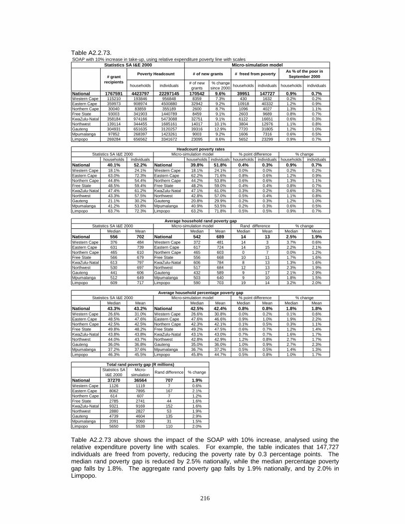
216
Table A2.2.73.
Table A2.2.73 above shows the impact of the SOAP with 10% increase, analysed using the relative expenditure poverty line with scales. For example, the table indicates that 147,727 individuals are freed from poverty, reducing the poverty rate by 0.3 percentage points. The median rand poverty gap is reduced by 2.5% nationally, while the median percentage poverty gap falls by 1.8%. The aggregate rand poverty gap falls by 1.9% nationally, and by 2.0% in Limpopo.
SOAP with 10% increase in take-up, using relative expenditure poverty line with scales
households individuals # of new grants
% change since 2000 households individuals households individuals
National 1767591 4423797 22297145 170542 9.6% 39951 147727 0.9% 0.7%Western Cape 115210 193846 956848 8359 7.3% 430 1632 0.2% 0.2%Eastern Cape 359973 908974 4500880 32942 9.2% 10918 40332 1.2% 0.9%Northern Cape 30040 83859 355189 2600 8.7% 1096 4027 1.3% 1.1%Free State 93003 341903 1440789 8459 9.1% 2603 9689 0.8% 0.7%KwaZulu-Natal 358184 974166 5473088 32751 9.1% 6122 16651 0.6% 0.3%Northwest 139114 344455 1685161 14017 10.1% 3804 12976 1.1% 0.8%Gauteng 304931 651635 3120257 39316 12.9% 7720 31805 1.2% 1.0%Mpumalanga 97852 268397 1423261 9003 9.2% 1606 7316 0.6% 0.5%Limpopo 269284 656562 3341672 23095 8.6% 5652 23299 0.9% 0.7%
households individuals households individuals households individuals households individualsNational 40.1% 52.2% National 39.8% 51.8% 0.4% 0.3% 0.9% 0.7%Western Cape 18.1% 24.1% Western Cape 18.1% 24.1% 0.0% 0.0% 0.2% 0.2%Eastern Cape 63.0% 72.3% Eastern Cape 62.2% 71.6% 0.8% 0.6% 1.2% 0.9%Northern Cape 44.8% 54.4% Northern Cape 44.2% 53.8% 0.6% 0.6% 1.3% 1.1%Free State 48.5% 59.4% Free State 48.2% 59.0% 0.4% 0.4% 0.8% 0.7%KwaZulu-Natal 47.4% 61.2% KwaZulu-Natal 47.1% 61.0% 0.3% 0.2% 0.6% 0.3%Northwest 43.3% 57.5% Northwest 42.8% 57.0% 0.5% 0.4% 1.1% 0.8%Gauteng 21.1% 30.2% Gauteng 20.8% 29.9% 0.2% 0.3% 1.2% 1.0%Mpumalanga 41.2% 53.8% Mpumalanga 40.9% 53.5% 0.2% 0.3% 0.6% 0.5%Limpopo 63.7% 72.3% Limpopo 63.2% 71.8% 0.5% 0.5% 0.9% 0.7%
Median Mean Median Mean Median Mean Median MeanNational 556 702 National 542 689 14 13 2.5% 1.9%Western Cape 376 484 Western Cape 372 481 14 3 3.7% 0.6%Eastern Cape 631 739 Eastern Cape 617 724 14 15 2.2% 2.1%Northern Cape 465 610 Northern Cape 465 603 0 7 0.0% 1.2%Free State 566 679 Free State 556 668 10 11 1.7% 1.6%KwaZulu-Natal 613 797 KwaZulu-Natal 606 784 8 13 1.3% 1.6%Northwest 530 697 Northwest 517 684 12 13 2.3% 1.9%Gauteng 441 606 Gauteng 432 589 9 17 2.1% 2.9%Mpumalanga 512 649 Mpumalanga 503 640 9 10 1.8% 1.5%Limpopo 609 717 Limpopo 590 703 19 14 3.2% 2.0%
Median Mean Median Mean Median Mean Median MeanNational 43.3% 43.2% National 42.5% 42.4% 0.8% 0.8% 1.8% 1.8%Western Cape 26.6% 31.0% Western Cape 26.6% 30.8% 0.0% 0.2% 0.1% 0.6%Eastern Cape 48.5% 47.6% Eastern Cape 47.6% 46.6% 0.9% 1.0% 1.9% 2.2%Northern Cape 42.5% 42.5% Northern Cape 42.3% 42.1% 0.1% 0.5% 0.3% 1.1%Free State 49.8% 48.2% Free State 49.2% 47.5% 0.6% 0.7% 1.2% 1.4%KwaZulu-Natal 43.8% 43.8% KwaZulu-Natal 43.1% 43.0% 0.7% 0.7% 1.6% 1.7%Northwest 44.0% 43.7% Northwest 42.8% 42.9% 1.2% 0.8% 2.7% 1.7%Gauteng 36.0% 36.8% Gauteng 35.0% 36.0% 1.0% 0.9% 2.7% 2.3%Mpumalanga 37.2% 37.6% Mpumalanga 36.7% 37.2% 0.5% 0.5% 1.4% 1.3%Limpopo 46.3% 45.5% Limpopo 45.8% 44.7% 0.5% 0.8% 1.0% 1.7%
Statistics SA I&E 2000
Micro-simulation Rand difference % change
National 37270 36564 707 1.9%Western Cape 1126 1119 7 0.6%Eastern Cape 8062 7895 167 2.1%Northern Cape 614 607 7 1.2%Free State 2785 2741 44 1.6%KwaZulu-Natal 9321 9169 152 1.6%Northwest 2880 2827 53 1.9%Gauteng 4739 4604 135 2.9%Mpumalanga 2091 2060 31 1.5%Limpopo 5650 5539 110 2.0%
Total rand poverty gap (R millions)
Statistics SA I&E 2000 Micro-simulation model
Micro-simulation modelStatistics SA I&E 2000
Poverty Headcount# grant
recipients
% point differenceAverage household percentage poverty gap
Average household rand poverty gap% change
% changeMicro-simulation model
% change
Headcount poverty rates
# of new grants # freed from poverty As % of the poor in September 2000
Statistics SA I&E 2000 % point difference
Statistics SA I&E 2000 Micro-simulation model Rand difference

217
Table A2.2.74.
Table A2.2.74 above shows the impact of the SOAP with full take up, analysed using the relative expenditure poverty line with scales. For example, the table indicates that 331,097 individuals are freed from poverty, reducing the poverty rate by 0.8 percentage points. The median rand poverty gap is reduced by 5.1% nationally, while the median percentage poverty gap falls by 3.4%. The aggregate rand poverty gap falls by 3.8% nationally, and by 3.0% in Limpopo.
SOAP with full take-up, using relative expenditure poverty line with scales
households individuals # of new grants
% change since 2000 households individuals households individuals
National 1767591 4423797 22297145 417730 23.6% 88168 331097 2.0% 1.5%Western Cape 115210 193846 956848 28838 25.0% 4720 12637 2.4% 1.3%Eastern Cape 359973 908974 4500880 80962 22.5% 23816 87080 2.6% 1.9%Northern Cape 30040 83859 355189 7490 24.9% 1783 5967 2.1% 1.7%Free State 93003 341903 1440789 22720 24.4% 5574 22978 1.6% 1.6%KwaZulu-Natal 358184 974166 5473088 87472 24.4% 18862 64256 1.9% 1.2%Northwest 139114 344455 1685161 28155 20.2% 7422 33559 2.2% 2.0%Gauteng 304931 651635 3120257 109732 36.0% 15465 66079 2.4% 2.1%Mpumalanga 97852 268397 1423261 12845 13.1% 1968 8764 0.7% 0.6%Limpopo 269284 656562 3341672 39516 14.7% 8558 29777 1.3% 0.9%
households individuals households individuals households individuals households individualsNational 40.1% 52.2% National 39.3% 51.4% 0.8% 0.8% 2.0% 1.5%Western Cape 18.1% 24.1% Western Cape 17.7% 23.8% 0.4% 0.3% 2.4% 1.3%Eastern Cape 63.0% 72.3% Eastern Cape 61.3% 70.9% 1.6% 1.4% 2.6% 1.9%Northern Cape 44.8% 54.4% Northern Cape 43.9% 53.5% 1.0% 0.9% 2.1% 1.7%Free State 48.5% 59.4% Free State 47.8% 58.5% 0.8% 0.9% 1.6% 1.6%KwaZulu-Natal 47.4% 61.2% KwaZulu-Natal 46.5% 60.5% 0.9% 0.7% 1.9% 1.2%Northwest 43.3% 57.5% Northwest 42.4% 56.3% 0.9% 1.1% 2.2% 2.0%Gauteng 21.1% 30.2% Gauteng 20.6% 29.6% 0.5% 0.6% 2.4% 2.1%Mpumalanga 41.2% 53.8% Mpumalanga 40.9% 53.5% 0.3% 0.3% 0.7% 0.6%Limpopo 63.7% 72.3% Limpopo 62.9% 71.7% 0.8% 0.6% 1.3% 0.9%
Median Mean Median Mean Median Mean Median MeanNational 556 702 National 528 676 28 26 5.1% 3.8%Western Cape 376 484 Western Cape 368 475 30 9 8.0% 1.9%Eastern Cape 631 739 Eastern Cape 601 708 30 31 4.7% 4.2%Northern Cape 465 610 Northern Cape 457 594 9 16 1.9% 2.6%Free State 566 679 Free State 541 654 25 25 4.5% 3.7%KwaZulu-Natal 613 797 KwaZulu-Natal 590 768 23 30 3.8% 3.7%Northwest 530 697 Northwest 499 671 30 26 5.7% 3.7%Gauteng 441 606 Gauteng 426 573 15 33 3.4% 5.4%Mpumalanga 512 649 Mpumalanga 499 637 12 12 2.4% 1.9%Limpopo 609 717 Limpopo 583 696 26 21 4.2% 3.0%
Median Mean Median Mean Median Mean Median MeanNational 43.3% 43.2% National 41.8% 41.6% 1.5% 1.6% 3.4% 3.7%Western Cape 26.6% 31.0% Western Cape 25.5% 30.0% 1.1% 1.0% 4.1% 3.2%Eastern Cape 48.5% 47.6% Eastern Cape 46.6% 45.5% 1.9% 2.1% 4.0% 4.4%Northern Cape 42.5% 42.5% Northern Cape 41.3% 41.4% 1.2% 1.1% 2.8% 2.7%Free State 49.8% 48.2% Free State 48.4% 46.6% 1.4% 1.6% 2.7% 3.3%KwaZulu-Natal 43.8% 43.8% KwaZulu-Natal 42.0% 42.0% 1.9% 1.7% 4.3% 3.9%Northwest 44.0% 43.7% Northwest 42.0% 42.2% 2.0% 1.5% 4.6% 3.5%Gauteng 36.0% 36.8% Gauteng 34.3% 35.2% 1.6% 1.6% 4.5% 4.4%Mpumalanga 37.2% 37.6% Mpumalanga 36.4% 37.0% 0.8% 0.7% 2.3% 1.7%Limpopo 46.3% 45.5% Limpopo 45.0% 44.2% 1.2% 1.3% 2.7% 2.9%
Statistics SA I&E 2000
Micro-simulation Rand difference % change
National 37270 35869 1401 3.8%Western Cape 1126 1104 22 1.9%Eastern Cape 8062 7722 340 4.2%Northern Cape 614 598 16 2.6%Free State 2785 2682 103 3.7%KwaZulu-Natal 9321 8972 348 3.7%Northwest 2880 2773 107 3.7%Gauteng 4739 4483 256 5.4%Mpumalanga 2091 2051 40 1.9%Limpopo 5650 5480 169 3.0%
Total rand poverty gap (R millions)
Statistics SA I&E 2000 Micro-simulation model
Micro-simulation modelStatistics SA I&E 2000
Poverty Headcount# grant
recipients
% point differenceAverage household percentage poverty gap
Average household rand poverty gap% change
% changeMicro-simulation model
% change
Headcount poverty rates
# of new grants # freed from poverty As % of the poor in September 2000
Statistics SA I&E 2000 % point difference
Statistics SA I&E 2000 Micro-simulation model Rand difference

218
TABLE A2.2.75.
Table A2.2.75 above shows the impact of the DG with 50% increase in take up, analysed using the relative expenditure poverty line with scales. For example, the table indicates that 195,233 individuals are freed from poverty, reducing the poverty rate by 0.5 percentage points. The median rand poverty gap is reduced by 3.2% nationally, while the median percentage poverty gap falls by 2.2%. The aggregate rand poverty gap falls by 2.6% nationally.
DG with 50% increase in take-up, using relative expenditure poverty line with scales
households individuals # of new grants
% change since 2000 households individuals households individuals
National 438542 4423797 22297145 218643 49.9% 50239 195233 1.1% 0.9%Western Cape 70442 193846 956848 14967 21.2% 3400 15864 1.8% 1.7%Eastern Cape 78664 908974 4500880 42630 54.2% 11283 38575 1.2% 0.9%Northern Cape 20076 83859 355189 6958 34.7% 1587 5720 1.9% 1.6%Free State 20069 341903 1440789 16374 81.6% 3051 9888 0.9% 0.7%KwaZulu-Natal 97038 974166 5473088 47750 49.2% 7713 36191 0.8% 0.7%Northwest 34942 344455 1685161 20419 58.4% 5922 19896 1.7% 1.2%Gauteng 61745 651635 3120257 33469 54.2% 9148 34571 1.4% 1.1%Mpumalanga 20091 268397 1423261 16801 83.6% 4836 23945 1.8% 1.7%Limpopo 35475 656562 3341672 19275 54.3% 3299 10583 0.5% 0.3%
households individuals households individuals households individuals households individualsNational 40.1% 52.2% National 39.7% 51.7% 0.5% 0.5% 1.1% 0.9%Western Cape 18.1% 24.1% Western Cape 17.8% 23.7% 0.3% 0.4% 1.8% 1.7%Eastern Cape 63.0% 72.3% Eastern Cape 62.2% 71.7% 0.8% 0.6% 1.2% 0.9%Northern Cape 44.8% 54.4% Northern Cape 44.0% 53.5% 0.8% 0.9% 1.9% 1.6%Free State 48.5% 59.4% Free State 48.1% 59.0% 0.4% 0.4% 0.9% 0.7%KwaZulu-Natal 47.4% 61.2% KwaZulu-Natal 47.0% 60.8% 0.4% 0.4% 0.8% 0.7%Northwest 43.3% 57.5% Northwest 42.6% 56.8% 0.7% 0.7% 1.7% 1.2%Gauteng 21.1% 30.2% Gauteng 20.8% 29.9% 0.3% 0.3% 1.4% 1.1%Mpumalanga 41.2% 53.8% Mpumalanga 40.4% 52.9% 0.8% 0.9% 2.0% 1.7%Limpopo 63.7% 72.3% Limpopo 63.4% 72.1% 0.3% 0.2% 0.5% 0.3%
Median Mean Median Mean Median Mean Median MeanNational 556 702 National 539 686 18 16 3.2% 2.3%Western Cape 376 484 Western Cape 360 471 20 13 5.4% 2.7%Eastern Cape 631 739 Eastern Cape 611 721 20 18 3.2% 2.4%Northern Cape 465 610 Northern Cape 454 587 11 23 2.5% 3.8%Free State 566 679 Free State 560 664 6 15 1.1% 2.2%KwaZulu-Natal 613 797 KwaZulu-Natal 605 780 8 17 1.3% 2.1%Northwest 530 697 Northwest 514 674 15 23 2.9% 3.3%Gauteng 441 606 Gauteng 432 594 9 12 2.1% 2.0%Mpumalanga 512 649 Mpumalanga 505 633 6 16 1.2% 2.5%Limpopo 609 717 Limpopo 586 705 23 12 3.8% 1.6%
Median Mean Median Mean Median Mean Median MeanNational 43.3% 43.2% National 42.3% 42.2% 0.9% 1.0% 2.2% 2.2%Western Cape 26.6% 31.0% Western Cape 25.6% 30.2% 1.0% 0.8% 3.7% 2.5%Eastern Cape 48.5% 47.6% Eastern Cape 47.0% 46.4% 1.5% 1.2% 3.1% 2.6%Northern Cape 42.5% 42.5% Northern Cape 40.8% 41.0% 1.7% 1.6% 3.9% 3.7%Free State 49.8% 48.2% Free State 48.9% 47.2% 0.9% 1.0% 1.8% 2.0%KwaZulu-Natal 43.8% 43.8% KwaZulu-Natal 43.2% 42.9% 0.7% 0.8% 1.5% 1.9%Northwest 44.0% 43.7% Northwest 42.2% 42.5% 1.8% 1.2% 4.1% 2.8%Gauteng 36.0% 36.8% Gauteng 34.9% 36.0% 1.1% 0.8% 2.9% 2.1%Mpumalanga 37.2% 37.6% Mpumalanga 36.5% 36.7% 0.7% 1.0% 1.9% 2.5%Limpopo 46.3% 45.5% Limpopo 45.6% 44.7% 0.7% 0.8% 1.4% 1.7%
Statistics SA I&E 2000
Micro-simulation Rand difference % change
National 37270 36319 952 2.6%Western Cape 1126 1096 30 2.7%Eastern Cape 8062 7852 210 2.6%Northern Cape 614 590 24 3.8%Free State 2785 2717 68 2.5%KwaZulu-Natal 9321 9080 240 2.6%Northwest 2880 2772 108 3.8%Gauteng 4739 4629 110 2.3%Mpumalanga 2091 2022 69 3.3%Limpopo 5650 5557 92 1.6%
% change
Headcount poverty rates
# of new grants # freed from poverty As % of the poor in September 2000
Statistics SA I&E 2000 % point difference
Statistics SA I&E 2000 Micro-simulation model Rand differenceAverage household rand poverty gap
% change
% changeMicro-simulation model
Total rand poverty gap (R millions)
Statistics SA I&E 2000 Micro-simulation model
Micro-simulation modelStatistics SA I&E 2000
Poverty Headcount# grant
recipients
% point differenceAverage household percentage poverty gap
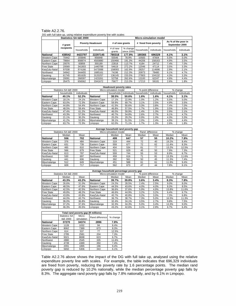
219
Table A2.2.76.
Table A2.2.76 above shows the impact of the DG with full take up, analysed using the relative expenditure poverty line with scales. For example, the table indicates that 696,329 individuals are freed from poverty, reducing the poverty rate by 1.6 percentage points. The median rand poverty gap is reduced by 10.2% nationally, while the median percentage poverty gap falls by 8.3%. The aggregate rand poverty gap falls by 7.8% nationally, and by 6.1% in Limpopo.
DG with full take-up, using relative expenditure poverty line with scales
households individuals # of new grants
% change since 2000 households individuals households individuals
National 438542 4423797 22297145 780318 177.9% 180365 696329 4.1% 3.1%Western Cape 70442 193846 956848 55546 78.9% 10583 47604 5.5% 5.0%Eastern Cape 78664 908974 4500880 150466 191.3% 44206 158163 4.9% 3.5%Northern Cape 20076 83859 355189 22818 113.7% 6184 24712 7.4% 7.0%Free State 20069 341903 1440789 54619 272.2% 12046 47114 3.5% 3.3%KwaZulu-Natal 97038 974166 5473088 158093 162.9% 28257 114696 2.9% 2.1%Northwest 34942 344455 1685161 74196 212.3% 20973 78480 6.1% 4.7%Gauteng 61745 651635 3120257 136145 220.5% 27803 104132 4.3% 3.3%Mpumalanga 20091 268397 1423261 52758 262.6% 13100 62247 4.9% 4.4%Limpopo 35475 656562 3341672 75677 213.3% 17213 59181 2.6% 1.8%
households individuals households individuals households individuals households individualsNational 40.1% 52.2% National 38.5% 50.6% 1.6% 1.6% 4.1% 3.1%Western Cape 18.1% 24.1% Western Cape 17.1% 22.9% 1.0% 1.2% 5.5% 5.0%Eastern Cape 63.0% 72.3% Eastern Cape 59.9% 69.7% 3.1% 2.5% 4.9% 3.5%Northern Cape 44.8% 54.4% Northern Cape 41.5% 50.6% 3.3% 3.8% 7.4% 7.0%Free State 48.5% 59.4% Free State 46.8% 57.5% 1.7% 1.9% 3.5% 3.3%KwaZulu-Natal 47.4% 61.2% KwaZulu-Natal 46.0% 59.9% 1.4% 1.3% 2.9% 2.1%Northwest 43.3% 57.5% Northwest 40.7% 54.8% 2.6% 2.7% 6.1% 4.7%Gauteng 21.1% 30.2% Gauteng 20.2% 29.2% 0.9% 1.0% 4.3% 3.3%Mpumalanga 41.2% 53.8% Mpumalanga 39.1% 51.5% 2.0% 2.4% 4.9% 4.4%Limpopo 63.7% 72.3% Limpopo 62.0% 71.1% 1.7% 1.3% 2.6% 1.8%
Median Mean Median Mean Median Mean Median MeanNational 556 702 National 499 647 57 55 10.2% 7.8%Western Cape 376 484 Western Cape 319 444 72 40 19.2% 8.4%Eastern Cape 631 739 Eastern Cape 559 677 72 62 11.4% 8.3%Northern Cape 465 610 Northern Cape 404 534 61 77 13.2% 12.5%Free State 566 679 Free State 521 629 45 50 7.9% 7.3%KwaZulu-Natal 613 797 KwaZulu-Natal 559 744 55 53 8.9% 6.7%Northwest 530 697 Northwest 459 616 71 81 13.3% 11.6%Gauteng 441 606 Gauteng 392 561 50 45 11.3% 7.4%Mpumalanga 512 649 Mpumalanga 451 588 61 61 11.9% 9.4%Limpopo 609 717 Limpopo 562 673 47 44 7.8% 6.1%
Median Mean Median Mean Median Mean Median MeanNational 43.3% 43.2% National 39.7% 39.8% 3.6% 3.4% 8.3% 7.8%Western Cape 26.6% 31.0% Western Cape 24.2% 28.5% 2.4% 2.5% 9.0% 8.0%Eastern Cape 48.5% 47.6% Eastern Cape 44.5% 43.6% 4.0% 4.0% 8.3% 8.5%Northern Cape 42.5% 42.5% Northern Cape 36.6% 37.6% 5.9% 4.9% 13.8% 11.6%Free State 49.8% 48.2% Free State 46.6% 44.9% 3.2% 3.2% 6.4% 6.7%KwaZulu-Natal 43.8% 43.8% KwaZulu-Natal 40.7% 40.8% 3.2% 3.0% 7.3% 6.8%Northwest 44.0% 43.7% Northwest 36.7% 38.7% 7.3% 5.0% 16.5% 11.3%Gauteng 36.0% 36.8% Gauteng 32.4% 34.1% 3.5% 2.7% 9.8% 7.5%Mpumalanga 37.2% 37.6% Mpumalanga 32.3% 34.3% 5.0% 3.4% 13.3% 9.0%Limpopo 46.3% 45.5% Limpopo 43.2% 42.6% 3.1% 2.9% 6.7% 6.4%
Statistics SA I&E 2000
Micro-simulation Rand difference % change
National 37270 34374 2896 7.8%Western Cape 1126 1032 94 8.4%Eastern Cape 8062 7389 673 8.3%Northern Cape 614 537 77 12.5%Free State 2785 2581 204 7.3%KwaZulu-Natal 9321 8698 623 6.7%Northwest 2880 2545 335 11.6%Gauteng 4739 4389 350 7.4%Mpumalanga 2091 1895 196 9.4%Limpopo 5650 5306 343 6.1%
% change
Headcount poverty rates
# of new grants # freed from poverty As % of the poor in September 2000
Statistics SA I&E 2000 % point difference
Statistics SA I&E 2000 Micro-simulation model Rand differenceAverage household rand poverty gap
% change
% changeMicro-simulation model
Total rand poverty gap (R millions)
Statistics SA I&E 2000 Micro-simulation model
Micro-simulation modelStatistics SA I&E 2000
Poverty Headcount# grant
recipients
% point differenceAverage household percentage poverty gap

220
Table A2.2.77.
Table A2.2.77 above shows the impact of the CSG at an annual level of R1200 in 2000, with full take up to the age 7, analysed using the relative expenditure poverty line with scales. For example, the table indicates that 863,256 individuals are freed from poverty, reducing the poverty rate by 2.0 percentage points. The median rand poverty gap is reduced by 12.4% nationally, while the median percentage poverty gap falls by 10.6%. The aggregate rand poverty gap falls by 10.7% nationally, and by 12.0% in Limpopo.
CSG to age 7 with full take-up, using relative expenditure poverty line with scales
households individuals # of new grants
% change since 2000 households individuals households individuals
National 463699 4423797 22297145 3458297 745.8% 166771 863256 3.8% 3.9%Western Cape 59407 193846 956848 143575 241.7% 17540 87688 9.0% 9.2%Eastern Cape 63038 908974 4500880 719919 1142.0% 20852 109699 2.3% 2.4%Northern Cape 19734 83859 355189 53904 273.2% 2476 13730 3.0% 3.9%Free State 18573 341903 1440789 185579 999.2% 5752 27132 1.7% 1.9%KwaZulu-Natal 70660 974166 5473088 920791 1303.1% 30881 161978 3.2% 3.0%Northwest 34341 344455 1685161 242082 704.9% 13664 69506 4.0% 4.1%Gauteng 107493 651635 3120257 405354 377.1% 42659 227927 6.5% 7.3%Mpumalanga 43704 268397 1423261 208019 476.0% 13664 66769 5.1% 4.7%Limpopo 46749 656562 3341672 579074 1238.7% 19283 98827 2.9% 3.0%
households individuals households individuals households individuals households individualsNational 40.1% 52.2% National 38.6% 50.2% 1.5% 2.0% 3.8% 3.9%Western Cape 18.1% 24.1% Western Cape 16.5% 21.9% 1.6% 2.2% 9.0% 9.2%Eastern Cape 63.0% 72.3% Eastern Cape 61.5% 70.5% 1.4% 1.8% 2.3% 2.4%Northern Cape 44.8% 54.4% Northern Cape 43.5% 52.3% 1.3% 2.1% 3.0% 3.9%Free State 48.5% 59.4% Free State 47.7% 58.3% 0.8% 1.1% 1.7% 1.9%KwaZulu-Natal 47.4% 61.2% KwaZulu-Natal 45.9% 59.4% 1.5% 1.8% 3.2% 3.0%Northwest 43.3% 57.5% Northwest 41.6% 55.1% 1.7% 2.4% 4.0% 4.1%Gauteng 21.1% 30.2% Gauteng 19.7% 28.0% 1.4% 2.2% 6.5% 7.3%Mpumalanga 41.2% 53.8% Mpumalanga 39.1% 51.3% 2.1% 2.5% 5.1% 4.7%Limpopo 63.7% 72.3% Limpopo 61.8% 70.2% 1.9% 2.1% 2.9% 3.0%
Median Mean Median Mean Median Mean Median MeanNational 556 702 National 487 627 69 75 12.4% 10.7%Western Cape 376 484 Western Cape 305 416 88 68 23.3% 14.0%Eastern Cape 631 739 Eastern Cape 544 661 88 78 13.9% 10.5%Northern Cape 465 610 Northern Cape 419 548 46 62 9.9% 10.2%Free State 566 679 Free State 523 626 43 53 7.6% 7.8%KwaZulu-Natal 613 797 KwaZulu-Natal 536 705 77 92 12.6% 11.5%Northwest 530 697 Northwest 465 629 64 67 12.1% 9.7%Gauteng 441 606 Gauteng 391 549 51 57 11.5% 9.4%Mpumalanga 512 649 Mpumalanga 454 576 58 73 11.4% 11.3%Limpopo 609 717 Limpopo 523 631 86 86 14.1% 12.0%
Median Mean Median Mean Median Mean Median MeanNational 43.3% 43.2% National 38.7% 38.9% 4.6% 4.3% 10.6% 9.9%Western Cape 26.6% 31.0% Western Cape 23.6% 26.8% 3.0% 4.2% 11.4% 13.4%Eastern Cape 48.5% 47.6% Eastern Cape 43.2% 43.0% 5.3% 4.6% 10.9% 9.7%Northern Cape 42.5% 42.5% Northern Cape 38.4% 38.7% 4.1% 3.9% 9.7% 9.1%Free State 49.8% 48.2% Free State 46.3% 44.7% 3.5% 3.5% 7.0% 7.3%KwaZulu-Natal 43.8% 43.8% KwaZulu-Natal 38.7% 39.1% 5.1% 4.7% 11.7% 10.7%Northwest 44.0% 43.7% Northwest 40.2% 40.0% 3.8% 3.7% 8.6% 8.5%Gauteng 36.0% 36.8% Gauteng 32.3% 33.5% 3.7% 3.3% 10.2% 8.9%Mpumalanga 37.2% 37.6% Mpumalanga 32.1% 33.6% 5.1% 4.1% 13.7% 10.8%Limpopo 46.3% 45.5% Limpopo 40.8% 40.5% 5.5% 5.0% 11.9% 11.0%
Statistics SA I&E 2000
Micro-simulation Rand difference % change
National 37270 33276 3995 10.7%Western Cape 1126 968 158 14.0%Eastern Cape 8062 7215 846 10.5%Northern Cape 614 552 62 10.2%Free State 2785 2567 218 7.8%KwaZulu-Natal 9321 8247 1073 11.5%Northwest 2880 2602 278 9.7%Gauteng 4739 4293 446 9.4%Mpumalanga 2091 1855 236 11.3%Limpopo 5650 4974 676 12.0%
% change
Headcount poverty rates
# of new grants # freed from poverty As % of the poor in September 2000
Statistics SA I&E 2000 % point difference
Statistics SA I&E 2000 Micro-simulation model Rand differenceAverage household rand poverty gap
% change
% changeMicro-simulation model
Total rand poverty gap (R millions)
Statistics SA I&E 2000 Micro-simulation model
Micro-simulation modelStatistics SA I&E 2000
Poverty Headcount# grant
recipients
% point differenceAverage household percentage poverty gap
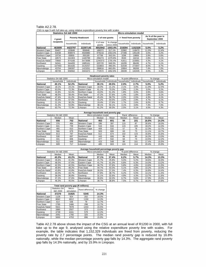
221
Table A2.2.78.
Table A2.2.78 above shows the impact of the CSG at an annual level of R1200 in 2000, with full take up to the age 9, analysed using the relative expenditure poverty line with scales. For example, the table indicates that 1,152,329 individuals are freed from poverty, reducing the poverty rate by 2.7 percentage points. The median rand poverty gap is reduced by 16.8% nationally, while the median percentage poverty gap falls by 14.3%. The aggregate rand poverty gap falls by 14.3% nationally, and by 15.9% in Limpopo.
CSG to age 9 with full take-up, using relative expenditure poverty line with scales
households individuals # of new grants
% change since 2000 households individuals households individuals
National 463699 4423797 22297145 4652942 1003.4% 219294 1152329 5.0% 5.2%Western Cape 59407 193846 956848 188372 317.1% 22982 118470 11.9% 12.4%Eastern Cape 63038 908974 4500880 979216 1553.4% 27396 145149 3.0% 3.2%Northern Cape 19734 83859 355189 67796 343.5% 3298 19806 3.9% 5.6%Free State 18573 341903 1440789 256274 1379.8% 9530 44216 2.8% 3.1%KwaZulu-Natal 70660 974166 5473088 1240373 1755.4% 41811 223691 4.3% 4.1%Northwest 34341 344455 1685161 325720 948.5% 16295 86436 4.7% 5.1%Gauteng 107493 651635 3120257 533803 496.6% 52039 272847 8.0% 8.7%Mpumalanga 43704 268397 1423261 288816 660.8% 19904 99269 7.4% 7.0%Limpopo 46749 656562 3341672 772572 1652.6% 26039 142445 4.0% 4.3%
households individuals households individuals households individuals households individualsNational 40.1% 52.2% National 38.1% 49.5% 2.0% 2.7% 5.0% 5.2%Western Cape 18.1% 24.1% Western Cape 16.0% 21.1% 2.1% 3.0% 11.9% 12.4%Eastern Cape 63.0% 72.3% Eastern Cape 61.1% 70.0% 1.9% 2.3% 3.0% 3.2%Northern Cape 44.8% 54.4% Northern Cape 43.0% 51.4% 1.8% 3.0% 3.9% 5.6%Free State 48.5% 59.4% Free State 47.2% 57.6% 1.4% 1.8% 2.8% 3.1%KwaZulu-Natal 47.4% 61.2% KwaZulu-Natal 45.4% 58.7% 2.0% 2.5% 4.3% 4.1%Northwest 43.3% 57.5% Northwest 41.2% 54.5% 2.0% 2.9% 4.7% 5.1%Gauteng 21.1% 30.2% Gauteng 19.4% 27.6% 1.7% 2.6% 8.0% 8.7%Mpumalanga 41.2% 53.8% Mpumalanga 38.1% 50.1% 3.1% 3.8% 7.4% 7.0%Limpopo 63.7% 72.3% Limpopo 61.2% 69.3% 2.5% 3.1% 4.0% 4.3%
Median Mean Median Mean Median Mean Median MeanNational 556 702 National 463 601 94 101 16.8% 14.3%Western Cape 376 484 Western Cape 286 397 115 87 30.6% 18.0%Eastern Cape 631 739 Eastern Cape 516 634 115 105 18.2% 14.3%Northern Cape 465 610 Northern Cape 408 532 57 78 12.3% 12.7%Free State 566 679 Free State 503 606 63 73 11.1% 10.7%KwaZulu-Natal 613 797 KwaZulu-Natal 512 674 102 123 16.6% 15.5%Northwest 530 697 Northwest 443 606 86 90 16.3% 13.0%Gauteng 441 606 Gauteng 377 532 64 74 14.5% 12.2%Mpumalanga 512 649 Mpumalanga 423 548 89 101 17.4% 15.5%Limpopo 609 717 Limpopo 485 603 124 114 20.4% 15.9%
Median Mean Median Mean Median Mean Median MeanNational 43.3% 43.2% National 37.1% 37.4% 6.2% 5.7% 14.3% 13.3%Western Cape 26.6% 31.0% Western Cape 21.7% 25.8% 5.0% 5.2% 18.6% 16.9%Eastern Cape 48.5% 47.6% Eastern Cape 41.7% 41.3% 6.8% 6.3% 14.0% 13.2%Northern Cape 42.5% 42.5% Northern Cape 36.7% 37.6% 5.8% 4.9% 13.6% 11.5%Free State 49.8% 48.2% Free State 44.7% 43.3% 5.1% 4.8% 10.2% 10.0%KwaZulu-Natal 43.8% 43.8% KwaZulu-Natal 36.5% 37.5% 7.4% 6.3% 16.8% 14.4%Northwest 44.0% 43.7% Northwest 37.8% 38.7% 6.2% 5.0% 14.1% 11.5%Gauteng 36.0% 36.8% Gauteng 31.1% 32.6% 4.9% 4.3% 13.7% 11.6%Mpumalanga 37.2% 37.6% Mpumalanga 30.6% 32.0% 6.7% 5.6% 17.9% 15.0%Limpopo 46.3% 45.5% Limpopo 38.7% 38.8% 7.5% 6.7% 16.3% 14.8%
Statistics SA I&E 2000
Micro-simulation Rand difference % change
National 37270 31925 5345 14.3%Western Cape 1126 924 202 18.0%Eastern Cape 8062 6912 1150 14.3%Northern Cape 614 536 78 12.7%Free State 2785 2486 298 10.7%KwaZulu-Natal 9321 7878 1443 15.5%Northwest 2880 2507 373 13.0%Gauteng 4739 4161 579 12.2%Mpumalanga 2091 1766 325 15.5%Limpopo 5650 4753 896 15.9%
% change
Headcount poverty rates
# of new grants # freed from poverty As % of the poor in September 2000
Statistics SA I&E 2000 % point difference
Statistics SA I&E 2000 Micro-simulation model Rand differenceAverage household rand poverty gap
% change
% changeMicro-simulation model
Total rand poverty gap (R millions)
Statistics SA I&E 2000 Micro-simulation model
Micro-simulation modelStatistics SA I&E 2000
Poverty Headcount# grant
recipients
% point differenceAverage household percentage poverty gap

222
Table A2.2.79.
Table A2.2.79 above shows the impact of the CSG at an annual level of R1200 in 2000, with full take up to the age 11, analysed using the relative expenditure poverty line with scales. For example, the table indicates that 1,513,462 individuals are freed from poverty, reducing the poverty rate by 3.5 percentage points. The median rand poverty gap is reduced by 21.0% nationally, while the median percentage poverty gap falls by 18.4%. The aggregate rand poverty gap falls by 18.1% nationally, and by 20.1% in Limpopo.
CSG to age 11 with full take-up, using relative expenditure poverty line with scales
households individuals # of new grants
% change since 2000 households individuals households individuals
National 463699 4423797 22297145 5898534 1272.1% 278995 1513462 6.3% 6.8%Western Cape 59407 193846 956848 242765 408.6% 28885 159461 14.9% 16.7%Eastern Cape 63038 908974 4500880 1261509 2001.2% 38106 190009 4.2% 4.2%Northern Cape 19734 83859 355189 84407 427.7% 4666 27311 5.6% 7.7%Free State 18573 341903 1440789 329032 1771.6% 10968 53042 3.2% 3.7%KwaZulu-Natal 70660 974166 5473088 1547232 2189.7% 53372 310085 5.5% 5.7%Northwest 34341 344455 1685161 418385 1218.3% 23374 127128 6.8% 7.5%Gauteng 107493 651635 3120257 659456 613.5% 58401 317639 9.0% 10.2%Mpumalanga 43704 268397 1423261 369237 844.9% 27775 143516 10.3% 10.1%Limpopo 46749 656562 3341672 986511 2110.2% 33448 185271 5.1% 5.5%
households individuals households individuals households individuals households individualsNational 40.1% 52.2% National 37.6% 48.6% 2.5% 3.5% 6.3% 6.8%Western Cape 18.1% 24.1% Western Cape 15.4% 20.1% 2.7% 4.0% 14.9% 16.7%Eastern Cape 63.0% 72.3% Eastern Cape 60.3% 69.2% 2.6% 3.1% 4.2% 4.2%Northern Cape 44.8% 54.4% Northern Cape 42.3% 50.2% 2.5% 4.2% 5.6% 7.7%Free State 48.5% 59.4% Free State 47.0% 57.2% 1.6% 2.2% 3.2% 3.7%KwaZulu-Natal 47.4% 61.2% KwaZulu-Natal 44.8% 57.8% 2.6% 3.5% 5.5% 5.7%Northwest 43.3% 57.5% Northwest 40.4% 53.1% 2.9% 4.3% 6.8% 7.5%Gauteng 21.1% 30.2% Gauteng 19.2% 27.2% 1.9% 3.1% 9.0% 10.2%Mpumalanga 41.2% 53.8% Mpumalanga 36.9% 48.4% 4.3% 5.4% 10.3% 10.1%Limpopo 63.7% 72.3% Limpopo 60.5% 68.3% 3.2% 4.0% 5.1% 5.5%
Median Mean Median Mean Median Mean Median MeanNational 556 702 National 440 575 117 127 21.0% 18.1%Western Cape 376 484 Western Cape 250 375 148 110 39.4% 22.6%Eastern Cape 631 739 Eastern Cape 483 604 148 135 23.5% 18.2%Northern Cape 465 610 Northern Cape 404 515 61 95 13.2% 15.6%Free State 566 679 Free State 488 585 78 93 13.8% 13.8%KwaZulu-Natal 613 797 KwaZulu-Natal 472 644 141 153 23.0% 19.2%Northwest 530 697 Northwest 428 582 101 115 19.1% 16.5%Gauteng 441 606 Gauteng 349 515 93 91 21.0% 15.0%Mpumalanga 512 649 Mpumalanga 407 521 105 128 20.6% 19.7%Limpopo 609 717 Limpopo 468 573 141 144 23.2% 20.1%
Median Mean Median Mean Median Mean Median MeanNational 43.3% 43.2% National 35.3% 36.0% 8.0% 7.2% 18.4% 16.7%Western Cape 26.6% 31.0% Western Cape 20.5% 24.3% 6.1% 6.7% 23.0% 21.5%Eastern Cape 48.5% 47.6% Eastern Cape 39.4% 39.5% 9.1% 8.1% 18.8% 17.0%Northern Cape 42.5% 42.5% Northern Cape 36.2% 36.6% 6.2% 5.9% 14.7% 14.0%Free State 49.8% 48.2% Free State 43.6% 42.0% 6.2% 6.1% 12.4% 12.7%KwaZulu-Natal 43.8% 43.8% KwaZulu-Natal 35.7% 35.9% 8.1% 7.8% 18.5% 17.9%Northwest 44.0% 43.7% Northwest 36.6% 37.3% 7.4% 6.4% 16.8% 14.7%Gauteng 36.0% 36.8% Gauteng 30.0% 31.7% 6.0% 5.1% 16.6% 14.0%Mpumalanga 37.2% 37.6% Mpumalanga 29.9% 30.5% 7.3% 7.1% 19.7% 19.0%Limpopo 46.3% 45.5% Limpopo 36.7% 37.0% 9.6% 8.6% 20.7% 18.8%
Statistics SA I&E 2000
Micro-simulation Rand difference % change
National 37270 30539 6731 18.1%Western Cape 1126 871 255 22.6%Eastern Cape 8062 6591 1471 18.2%Northern Cape 614 518 96 15.6%Free State 2785 2402 383 13.8%KwaZulu-Natal 9321 7531 1790 19.2%Northwest 2880 2405 475 16.5%Gauteng 4739 4027 713 15.0%Mpumalanga 2091 1679 412 19.7%Limpopo 5650 4513 1137 20.1%
% change
Headcount poverty rates
# of new grants # freed from poverty As % of the poor in September 2000
Statistics SA I&E 2000 % point difference
Statistics SA I&E 2000 Micro-simulation model Rand differenceAverage household rand poverty gap
% change
% changeMicro-simulation model
Total rand poverty gap (R millions)
Statistics SA I&E 2000 Micro-simulation model
Micro-simulation modelStatistics SA I&E 2000
Poverty Headcount# grant
recipients
% point differenceAverage household percentage poverty gap
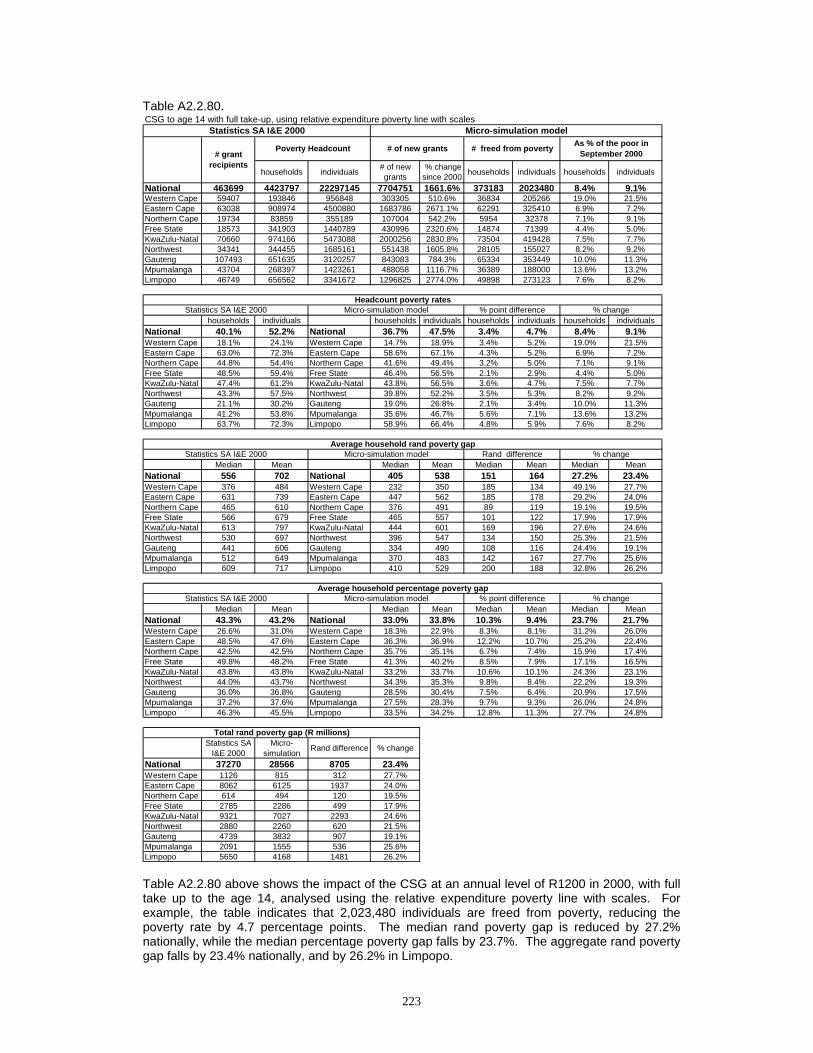
223
Table A2.2.80.
Table A2.2.80 above shows the impact of the CSG at an annual level of R1200 in 2000, with full take up to the age 14, analysed using the relative expenditure poverty line with scales. For example, the table indicates that 2,023,480 individuals are freed from poverty, reducing the poverty rate by 4.7 percentage points. The median rand poverty gap is reduced by 27.2% nationally, while the median percentage poverty gap falls by 23.7%. The aggregate rand poverty gap falls by 23.4% nationally, and by 26.2% in Limpopo.
CSG to age 14 with full take-up, using relative expenditure poverty line with scales
households individuals # of new grants
% change since 2000 households individuals households individuals
National 463699 4423797 22297145 7704751 1661.6% 373183 2023480 8.4% 9.1%Western Cape 59407 193846 956848 303305 510.6% 36834 205266 19.0% 21.5%Eastern Cape 63038 908974 4500880 1683786 2671.1% 62291 325410 6.9% 7.2%Northern Cape 19734 83859 355189 107004 542.2% 5954 32378 7.1% 9.1%Free State 18573 341903 1440789 430996 2320.6% 14874 71399 4.4% 5.0%KwaZulu-Natal 70660 974166 5473088 2000256 2830.8% 73504 419428 7.5% 7.7%Northwest 34341 344455 1685161 551438 1605.8% 28105 155027 8.2% 9.2%Gauteng 107493 651635 3120257 843083 784.3% 65334 353449 10.0% 11.3%Mpumalanga 43704 268397 1423261 488058 1116.7% 36389 188000 13.6% 13.2%Limpopo 46749 656562 3341672 1296825 2774.0% 49898 273123 7.6% 8.2%
households individuals households individuals households individuals households individualsNational 40.1% 52.2% National 36.7% 47.5% 3.4% 4.7% 8.4% 9.1%Western Cape 18.1% 24.1% Western Cape 14.7% 18.9% 3.4% 5.2% 19.0% 21.5%Eastern Cape 63.0% 72.3% Eastern Cape 58.6% 67.1% 4.3% 5.2% 6.9% 7.2%Northern Cape 44.8% 54.4% Northern Cape 41.6% 49.4% 3.2% 5.0% 7.1% 9.1%Free State 48.5% 59.4% Free State 46.4% 56.5% 2.1% 2.9% 4.4% 5.0%KwaZulu-Natal 47.4% 61.2% KwaZulu-Natal 43.8% 56.5% 3.6% 4.7% 7.5% 7.7%Northwest 43.3% 57.5% Northwest 39.8% 52.2% 3.5% 5.3% 8.2% 9.2%Gauteng 21.1% 30.2% Gauteng 19.0% 26.8% 2.1% 3.4% 10.0% 11.3%Mpumalanga 41.2% 53.8% Mpumalanga 35.6% 46.7% 5.6% 7.1% 13.6% 13.2%Limpopo 63.7% 72.3% Limpopo 58.9% 66.4% 4.8% 5.9% 7.6% 8.2%
Median Mean Median Mean Median Mean Median MeanNational 556 702 National 405 538 151 164 27.2% 23.4%Western Cape 376 484 Western Cape 232 350 185 134 49.1% 27.7%Eastern Cape 631 739 Eastern Cape 447 562 185 178 29.2% 24.0%Northern Cape 465 610 Northern Cape 376 491 89 119 19.1% 19.5%Free State 566 679 Free State 465 557 101 122 17.9% 17.9%KwaZulu-Natal 613 797 KwaZulu-Natal 444 601 169 196 27.6% 24.6%Northwest 530 697 Northwest 396 547 134 150 25.3% 21.5%Gauteng 441 606 Gauteng 334 490 108 116 24.4% 19.1%Mpumalanga 512 649 Mpumalanga 370 483 142 167 27.7% 25.6%Limpopo 609 717 Limpopo 410 529 200 188 32.8% 26.2%
Median Mean Median Mean Median Mean Median MeanNational 43.3% 43.2% National 33.0% 33.8% 10.3% 9.4% 23.7% 21.7%Western Cape 26.6% 31.0% Western Cape 18.3% 22.9% 8.3% 8.1% 31.2% 26.0%Eastern Cape 48.5% 47.6% Eastern Cape 36.3% 36.9% 12.2% 10.7% 25.2% 22.4%Northern Cape 42.5% 42.5% Northern Cape 35.7% 35.1% 6.7% 7.4% 15.9% 17.4%Free State 49.8% 48.2% Free State 41.3% 40.2% 8.5% 7.9% 17.1% 16.5%KwaZulu-Natal 43.8% 43.8% KwaZulu-Natal 33.2% 33.7% 10.6% 10.1% 24.3% 23.1%Northwest 44.0% 43.7% Northwest 34.3% 35.3% 9.8% 8.4% 22.2% 19.3%Gauteng 36.0% 36.8% Gauteng 28.5% 30.4% 7.5% 6.4% 20.9% 17.5%Mpumalanga 37.2% 37.6% Mpumalanga 27.5% 28.3% 9.7% 9.3% 26.0% 24.8%Limpopo 46.3% 45.5% Limpopo 33.5% 34.2% 12.8% 11.3% 27.7% 24.8%
Statistics SA I&E 2000
Micro-simulation Rand difference % change
National 37270 28566 8705 23.4%Western Cape 1126 815 312 27.7%Eastern Cape 8062 6125 1937 24.0%Northern Cape 614 494 120 19.5%Free State 2785 2286 499 17.9%KwaZulu-Natal 9321 7027 2293 24.6%Northwest 2880 2260 620 21.5%Gauteng 4739 3832 907 19.1%Mpumalanga 2091 1555 536 25.6%Limpopo 5650 4168 1481 26.2%
% change
Headcount poverty rates
# of new grants # freed from poverty As % of the poor in September 2000
Statistics SA I&E 2000 % point difference
Statistics SA I&E 2000 Micro-simulation model Rand differenceAverage household rand poverty gap
% change
% changeMicro-simulation model
Total rand poverty gap (R millions)
Statistics SA I&E 2000 Micro-simulation model
Micro-simulation modelStatistics SA I&E 2000
Poverty Headcount# grant
recipients
% point differenceAverage household percentage poverty gap
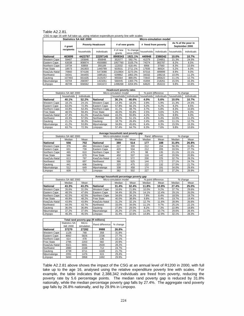
224
Table A2.2.81.
Table A2.2.81 above shows the impact of the CSG at an annual level of R1200 in 2000, with full take up to the age 16, analysed using the relative expenditure poverty line with scales. For example, the table indicates that 2,388,342 individuals are freed from poverty, reducing the poverty rate by 5.6 percentage points. The median rand poverty gap is reduced by 31.8% nationally, while the median percentage poverty gap falls by 27.4%. The aggregate rand poverty gap falls by 26.8% nationally, and by 29.9% in Limpopo.
CSG to age 16 with full take-up, using relative expenditure poverty line with scales
households individuals # of new grants
% change since 2000 households individuals households individuals
National 463699 4423797 22297145 8908343 1921.1% 440948 2388342 10.0% 10.7%Western Cape 59407 193846 956848 352077 592.7% 41379 234851 21.3% 24.5%Eastern Cape 63038 908974 4500880 1957760 3105.7% 74374 383787 8.2% 8.5%Northern Cape 19734 83859 355189 122032 618.4% 6956 37560 8.3% 10.6%Free State 18573 341903 1440789 503531 2711.1% 17935 86924 5.2% 6.0%KwaZulu-Natal 70660 974166 5473088 2310804 3270.3% 87016 489899 8.9% 9.0%Northwest 34341 344455 1685161 639862 1863.3% 34332 188216 10.0% 11.2%Gauteng 107493 651635 3120257 955564 889.0% 72642 395622 11.1% 12.7%Mpumalanga 43704 268397 1423261 568445 1300.7% 41694 218261 15.5% 15.3%Limpopo 46749 656562 3341672 1498268 3204.9% 64620 353222 9.8% 10.6%
households individuals households individuals households individuals households individualsNational 40.1% 52.2% National 36.1% 46.6% 4.0% 5.6% 10.0% 10.7%Western Cape 18.1% 24.1% Western Cape 14.3% 18.2% 3.9% 5.9% 21.3% 24.5%Eastern Cape 63.0% 72.3% Eastern Cape 57.8% 66.1% 5.2% 6.2% 8.2% 8.5%Northern Cape 44.8% 54.4% Northern Cape 41.1% 48.7% 3.7% 5.8% 8.3% 10.6%Free State 48.5% 59.4% Free State 46.0% 55.8% 2.5% 3.6% 5.2% 6.0%KwaZulu-Natal 47.4% 61.2% KwaZulu-Natal 43.2% 55.8% 4.2% 5.5% 8.9% 9.0%Northwest 43.3% 57.5% Northwest 39.0% 51.1% 4.3% 6.4% 10.0% 11.2%Gauteng 21.1% 30.2% Gauteng 18.7% 26.4% 2.4% 3.8% 11.1% 12.7%Mpumalanga 41.2% 53.8% Mpumalanga 34.8% 45.6% 6.4% 8.3% 15.5% 15.3%Limpopo 63.7% 72.3% Limpopo 57.4% 64.7% 6.3% 7.6% 9.8% 10.6%
Median Mean Median Mean Median Mean Median MeanNational 556 702 National 380 514 177 188 31.8% 26.8%Western Cape 376 484 Western Cape 217 330 212 154 56.3% 31.8%Eastern Cape 631 739 Eastern Cape 420 534 212 205 33.5% 27.7%Northern Cape 465 610 Northern Cape 367 475 98 135 21.1% 22.1%Free State 566 679 Free State 450 537 116 142 20.5% 20.9%KwaZulu-Natal 613 797 KwaZulu-Natal 413 572 200 225 32.7% 28.2%Northwest 530 697 Northwest 386 525 144 172 27.1% 24.7%Gauteng 441 606 Gauteng 320 475 122 132 27.5% 21.7%Mpumalanga 512 649 Mpumalanga 338 458 174 191 34.0% 29.4%Limpopo 609 717 Limpopo 382 502 227 215 37.2% 29.9%
Median Mean Median Mean Median Mean Median MeanNational 43.3% 43.2% National 31.4% 32.4% 11.8% 10.8% 27.4% 25.0%Western Cape 26.6% 31.0% Western Cape 16.6% 21.8% 10.0% 9.2% 37.7% 29.6%Eastern Cape 48.5% 47.6% Eastern Cape 34.4% 35.2% 14.1% 12.4% 29.1% 26.0%Northern Cape 42.5% 42.5% Northern Cape 34.6% 34.1% 7.8% 8.4% 18.5% 19.7%Free State 49.8% 48.2% Free State 40.0% 38.8% 9.8% 9.4% 19.7% 19.4%KwaZulu-Natal 43.8% 43.8% KwaZulu-Natal 31.2% 32.1% 12.7% 11.6% 28.9% 26.6%Northwest 44.0% 43.7% Northwest 33.0% 34.0% 11.1% 9.7% 25.1% 22.1%Gauteng 36.0% 36.8% Gauteng 27.8% 29.5% 8.2% 7.3% 22.9% 19.8%Mpumalanga 37.2% 37.6% Mpumalanga 26.2% 27.0% 11.0% 10.7% 29.6% 28.4%Limpopo 46.3% 45.5% Limpopo 31.4% 32.6% 14.8% 12.9% 32.1% 28.3%
Statistics SA I&E 2000
Micro-simulation Rand difference % change
National 37270 27282 9988 26.8%Western Cape 1126 768 358 31.8%Eastern Cape 8062 5826 2236 27.7%Northern Cape 614 478 136 22.1%Free State 2785 2203 582 20.9%KwaZulu-Natal 9321 6691 2630 28.2%Northwest 2880 2168 712 24.7%Gauteng 4739 3711 1028 21.7%Mpumalanga 2091 1476 615 29.4%Limpopo 5650 3958 1692 29.9%
% change
Headcount poverty rates
# of new grants # freed from poverty As % of the poor in September 2000
Statistics SA I&E 2000 % point difference
Statistics SA I&E 2000 Micro-simulation model Rand differenceAverage household rand poverty gap
% change
% changeMicro-simulation model
Total rand poverty gap (R millions)
Statistics SA I&E 2000 Micro-simulation model
Micro-simulation modelStatistics SA I&E 2000
Poverty Headcount# grant
recipients
% point differenceAverage household percentage poverty gap

225
Table A2.2.82.
Table A2.2.82 above shows the impact of the CSG at an annual level of R1200 in 2000, with full take up to the age 18, analysed using the relative expenditure poverty line with scales. For example, the table indicates that 2,755,081 individuals are freed from poverty, reducing the poverty rate by 6.4 percentage points. The median rand poverty gap is reduced by 34.3% nationally, while the median percentage poverty gap falls by 30.5%. The aggregate rand poverty gap falls by 29.9% nationally, and by 33.3% in Limpopo.
CSG to age 18 with full take-up, using relative expenditure poverty line with scales
households individuals # of new grants
% change since 2000 households individuals households individuals
National 463699 4423797 22297145 10004785 2157.6% 511311 2755081 11.6% 12.4%Western Cape 59407 193846 956848 394058 663.3% 45637 259460 23.5% 27.1%Eastern Cape 63038 908974 4500880 2207293 3501.5% 93614 473718 10.3% 10.5%Northern Cape 19734 83859 355189 135505 686.7% 7695 41702 9.2% 11.7%Free State 18573 341903 1440789 578117 3112.7% 21586 104634 6.3% 7.3%KwaZulu-Natal 70660 974166 5473088 2584348 3657.4% 100183 561953 10.3% 10.3%Northwest 34341 344455 1685161 712385 2074.4% 37703 206793 10.9% 12.3%Gauteng 107493 651635 3120257 1067394 993.0% 80865 440491 12.4% 14.1%Mpumalanga 43704 268397 1423261 646154 1478.5% 46974 248759 17.5% 17.5%Limpopo 46749 656562 3341672 1679531 3592.7% 77054 417571 11.7% 12.5%
households individuals households individuals households individuals households individualsNational 40.1% 52.2% National 35.5% 45.7% 4.6% 6.4% 11.6% 12.4%Western Cape 18.1% 24.1% Western Cape 13.9% 17.6% 4.3% 6.5% 23.5% 27.1%Eastern Cape 63.0% 72.3% Eastern Cape 56.5% 64.7% 6.5% 7.6% 10.3% 10.5%Northern Cape 44.8% 54.4% Northern Cape 40.7% 48.0% 4.1% 6.4% 9.2% 11.7%Free State 48.5% 59.4% Free State 45.5% 55.1% 3.1% 4.3% 6.3% 7.3%KwaZulu-Natal 47.4% 61.2% KwaZulu-Natal 42.5% 54.9% 4.9% 6.3% 10.3% 10.3%Northwest 43.3% 57.5% Northwest 38.6% 50.4% 4.7% 7.1% 10.9% 12.3%Gauteng 21.1% 30.2% Gauteng 18.5% 26.0% 2.6% 4.3% 12.4% 14.1%Mpumalanga 41.2% 53.8% Mpumalanga 34.0% 44.4% 7.2% 9.4% 17.5% 17.5%Limpopo 63.7% 72.3% Limpopo 56.2% 63.3% 7.5% 9.0% 11.7% 12.5%
Median Mean Median Mean Median Mean Median MeanNational 556 702 National 366 492 191 210 34.3% 29.9%Western Cape 376 484 Western Cape 197 315 234 169 62.3% 35.0%Eastern Cape 631 739 Eastern Cape 397 510 234 229 37.1% 31.0%Northern Cape 465 610 Northern Cape 364 461 101 149 21.8% 24.4%Free State 566 679 Free State 440 517 126 162 22.3% 23.9%KwaZulu-Natal 613 797 KwaZulu-Natal 386 547 227 250 37.0% 31.4%Northwest 530 697 Northwest 377 507 153 190 28.8% 27.3%Gauteng 441 606 Gauteng 314 460 128 146 29.0% 24.2%Mpumalanga 512 649 Mpumalanga 314 434 197 215 38.6% 33.2%Limpopo 609 717 Limpopo 366 479 244 239 40.0% 33.3%
Median Mean Median Mean Median Mean Median MeanNational 43.3% 43.2% National 30.1% 31.1% 13.2% 12.0% 30.5% 27.9%Western Cape 26.6% 31.0% Western Cape 15.8% 21.0% 10.8% 10.0% 40.5% 32.3%Eastern Cape 48.5% 47.6% Eastern Cape 33.3% 33.7% 15.2% 13.9% 31.2% 29.2%Northern Cape 42.5% 42.5% Northern Cape 34.0% 33.3% 8.4% 9.3% 19.9% 21.8%Free State 49.8% 48.2% Free State 38.5% 37.3% 11.3% 10.8% 22.7% 22.5%KwaZulu-Natal 43.8% 43.8% KwaZulu-Natal 29.8% 30.8% 14.0% 12.9% 31.9% 29.5%Northwest 44.0% 43.7% Northwest 31.9% 33.0% 12.2% 10.7% 27.6% 24.5%Gauteng 36.0% 36.8% Gauteng 26.7% 28.7% 9.3% 8.1% 25.9% 21.9%Mpumalanga 37.2% 37.6% Mpumalanga 24.8% 25.6% 12.5% 12.0% 33.5% 31.9%Limpopo 46.3% 45.5% Limpopo 29.5% 31.2% 16.8% 14.4% 36.2% 31.5%
Statistics SA I&E 2000
Micro-simulation Rand difference % change
National 37270 26128 11143 29.9%Western Cape 1126 732 394 35.0%Eastern Cape 8062 5560 2502 31.0%Northern Cape 614 464 150 24.4%Free State 2785 2119 666 23.9%KwaZulu-Natal 9321 6394 2926 31.4%Northwest 2880 2094 786 27.3%Gauteng 4739 3594 1145 24.2%Mpumalanga 2091 1397 694 33.2%Limpopo 5650 3770 1879 33.3%
% change
Headcount poverty rates
# of new grants # freed from poverty As % of the poor in September 2000
Statistics SA I&E 2000 % point difference
Statistics SA I&E 2000 Micro-simulation model Rand differenceAverage household rand poverty gap
% change
% changeMicro-simulation model
Total rand poverty gap (R millions)
Statistics SA I&E 2000 Micro-simulation model
Micro-simulation modelStatistics SA I&E 2000
Poverty Headcount# grant
recipients
% point differenceAverage household percentage poverty gap

226
Table A2.2.83.
Table A2.2.83 above shows the impact of the CSG at an annual level of R1606 in 2000, with full take up to the age 7, analysed using the relative expenditure poverty line with scales. For example, the table indicates that 1,175,154 individuals are freed from poverty, reducing the poverty rate by 2.8 percentage points. The median rand poverty gap is reduced by 16.0% nationally, while the median percentage poverty gap falls by 14.1%. The aggregate rand poverty gap falls by 14.1% nationally, and by 15.8% in Limpopo.
CSG(1606) to age 7 with full take-up, using relative expenditure poverty line with scales
households individuals # of new grants
% change since 2000 households individuals households individuals
National 463699 4423797 22297145 3458297 745.8% 223168 1175154 5.0% 5.3%Western Cape 59407 193846 956848 143575 241.7% 22769 124437 11.7% 13.0%Eastern Cape 63038 908974 4500880 719919 1142.0% 29287 144618 3.2% 3.2%Northern Cape 19734 83859 355189 53904 273.2% 3511 18037 4.2% 5.1%Free State 18573 341903 1440789 185579 999.2% 7609 35670 2.2% 2.5%KwaZulu-Natal 70660 974166 5473088 920791 1303.1% 41622 224511 4.3% 4.1%Northwest 34341 344455 1685161 242082 704.9% 17876 98051 5.2% 5.8%Gauteng 107493 651635 3120257 405354 377.1% 51066 268393 7.8% 8.6%Mpumalanga 43704 268397 1423261 208019 476.0% 19756 103308 7.4% 7.3%Limpopo 46749 656562 3341672 579074 1238.7% 29672 158129 4.5% 4.7%
households individuals households individuals households individuals households individualsNational 40.1% 52.2% National 38.1% 49.4% 2.0% 2.8% 5.0% 5.3%Western Cape 18.1% 24.1% Western Cape 16.0% 21.0% 2.1% 3.1% 11.7% 13.0%Eastern Cape 63.0% 72.3% Eastern Cape 60.9% 70.0% 2.0% 2.3% 3.2% 3.2%Northern Cape 44.8% 54.4% Northern Cape 42.9% 51.6% 1.9% 2.8% 4.2% 5.1%Free State 48.5% 59.4% Free State 47.5% 57.9% 1.1% 1.5% 2.2% 2.5%KwaZulu-Natal 47.4% 61.2% KwaZulu-Natal 45.4% 58.7% 2.0% 2.5% 4.3% 4.1%Northwest 43.3% 57.5% Northwest 41.0% 54.1% 2.2% 3.3% 5.2% 5.8%Gauteng 21.1% 30.2% Gauteng 19.4% 27.6% 1.7% 2.6% 7.8% 8.6%Mpumalanga 41.2% 53.8% Mpumalanga 38.1% 49.9% 3.0% 3.9% 7.4% 7.3%Limpopo 63.7% 72.3% Limpopo 60.8% 68.9% 2.9% 3.4% 4.5% 4.7%
Median Mean Median Mean Median Mean Median MeanNational 556 702 National 467 603 89 99 16.0% 14.1%Western Cape 376 484 Western Cape 285 396 118 88 31.5% 18.2%Eastern Cape 631 739 Eastern Cape 513 636 118 103 18.8% 13.9%Northern Cape 465 610 Northern Cape 406 529 60 81 12.8% 13.3%Free State 566 679 Free State 513 608 54 71 9.5% 10.4%KwaZulu-Natal 613 797 KwaZulu-Natal 509 676 105 122 17.1% 15.3%Northwest 530 697 Northwest 442 608 88 89 16.6% 12.7%Gauteng 441 606 Gauteng 377 532 65 74 14.7% 12.3%Mpumalanga 512 649 Mpumalanga 427 553 84 96 16.5% 14.8%Limpopo 609 717 Limpopo 498 604 111 113 18.3% 15.8%
Median Mean Median Mean Median Mean Median MeanNational 43.3% 43.2% National 37.2% 37.6% 6.1% 5.6% 14.1% 13.0%Western Cape 26.6% 31.0% Western Cape 22.4% 25.6% 4.2% 5.4% 15.9% 17.4%Eastern Cape 48.5% 47.6% Eastern Cape 41.4% 41.5% 7.1% 6.1% 14.7% 12.9%Northern Cape 42.5% 42.5% Northern Cape 36.6% 37.4% 5.9% 5.1% 13.8% 11.9%Free State 49.8% 48.2% Free State 45.2% 43.5% 4.6% 4.6% 9.3% 9.6%KwaZulu-Natal 43.8% 43.8% KwaZulu-Natal 37.0% 37.6% 6.8% 6.2% 15.5% 14.1%Northwest 44.0% 43.7% Northwest 39.0% 38.8% 5.0% 4.9% 11.4% 11.1%Gauteng 36.0% 36.8% Gauteng 31.2% 32.5% 4.8% 4.3% 13.2% 11.6%Mpumalanga 37.2% 37.6% Mpumalanga 31.0% 32.3% 6.2% 5.3% 16.7% 14.1%Limpopo 46.3% 45.5% Limpopo 39.0% 38.9% 7.3% 6.6% 15.8% 14.5%
Statistics SA I&E 2000
Micro-simulation Rand difference % change
National 37270 31998 5272 14.1%Western Cape 1126 921 205 18.2%Eastern Cape 8062 6940 1121 13.9%Northern Cape 614 532 82 13.3%Free State 2785 2495 289 10.4%KwaZulu-Natal 9321 7898 1423 15.3%Northwest 2880 2514 366 12.7%Gauteng 4739 4157 582 12.3%Mpumalanga 2091 1781 310 14.8%Limpopo 5650 4756 894 15.8%
Total rand poverty gap (R millions)
Statistics SA I&E 2000 Micro-simulation model
Micro-simulation modelStatistics SA I&E 2000
Poverty Headcount# grant
recipients
% point differenceAverage household percentage poverty gap
Average household rand poverty gap% change
% changeMicro-simulation model
% change
Headcount poverty rates
# of new grants # freed from poverty As % of the poor in September 2000
Statistics SA I&E 2000 % point difference
Statistics SA I&E 2000 Micro-simulation model Rand difference

227
Table A2.2.84.
Table A2.2.84 above shows the impact of the CSG at an annual level of R1606 in 2000, with full take up to the age 9, analysed using the relative expenditure poverty line with scales. For example, the table indicates that 1,650,419 individuals are freed from poverty, reducing the poverty rate by 3.9 percentage points. The median rand poverty gap is reduced by 21.8% nationally, while the median percentage poverty gap falls by 18.9%. The aggregate rand poverty gap falls by 18.9% nationally, and by 20.9% in Limpopo.
CSG(1606) to age 9 with full take-up, using relative expenditure poverty line with scales
households individuals # of new grants
% change since 2000 households individuals households individuals
National 463699 4423797 22297145 4652942 1003.4% 306770 1650419 6.9% 7.4%Western Cape 59407 193846 956848 188372 317.1% 31100 172674 16.0% 18.0%Eastern Cape 63038 908974 4500880 979216 1553.4% 43893 232579 4.8% 5.2%Northern Cape 19734 83859 355189 67796 343.5% 4928 27307 5.9% 7.7%Free State 18573 341903 1440789 256274 1379.8% 11997 54612 3.5% 3.8%KwaZulu-Natal 70660 974166 5473088 1240373 1755.4% 60320 345882 6.2% 6.3%Northwest 34341 344455 1685161 325720 948.5% 22021 127754 6.4% 7.6%Gauteng 107493 651635 3120257 533803 496.6% 63587 331719 9.8% 10.6%Mpumalanga 43704 268397 1423261 288816 660.8% 28143 140441 10.5% 9.9%Limpopo 46749 656562 3341672 772572 1652.6% 40781 217451 6.2% 6.5%
households individuals households individuals households individuals households individualsNational 40.1% 52.2% National 37.3% 48.3% 2.8% 3.9% 6.9% 7.4%Western Cape 18.1% 24.1% Western Cape 15.2% 19.8% 2.9% 4.4% 16.0% 18.0%Eastern Cape 63.0% 72.3% Eastern Cape 59.9% 68.6% 3.0% 3.7% 4.8% 5.2%Northern Cape 44.8% 54.4% Northern Cape 42.2% 50.2% 2.6% 4.2% 5.9% 7.7%Free State 48.5% 59.4% Free State 46.8% 57.1% 1.7% 2.3% 3.5% 3.8%KwaZulu-Natal 47.4% 61.2% KwaZulu-Natal 44.5% 57.4% 2.9% 3.9% 6.2% 6.3%Northwest 43.3% 57.5% Northwest 40.5% 53.1% 2.8% 4.4% 6.4% 7.6%Gauteng 21.1% 30.2% Gauteng 19.0% 27.0% 2.1% 3.2% 9.8% 10.6%Mpumalanga 41.2% 53.8% Mpumalanga 36.8% 48.5% 4.3% 5.3% 10.5% 9.9%Limpopo 63.7% 72.3% Limpopo 59.8% 67.6% 4.0% 4.7% 6.2% 6.5%
Median Mean Median Mean Median Mean Median MeanNational 556 702 National 435 570 121 132 21.8% 18.9%Western Cape 376 484 Western Cape 252 373 151 111 40.0% 22.9%Eastern Cape 631 739 Eastern Cape 481 600 151 139 23.8% 18.8%Northern Cape 465 610 Northern Cape 391 509 74 101 15.9% 16.6%Free State 566 679 Free State 484 583 83 96 14.6% 14.2%KwaZulu-Natal 613 797 KwaZulu-Natal 472 634 142 163 23.1% 20.4%Northwest 530 697 Northwest 414 578 116 119 21.9% 17.1%Gauteng 441 606 Gauteng 359 510 82 96 18.7% 15.9%Mpumalanga 512 649 Mpumalanga 388 517 124 132 24.2% 20.3%Limpopo 609 717 Limpopo 451 567 159 150 26.0% 20.9%
Median Mean Median Mean Median Mean Median MeanNational 43.3% 43.2% National 35.1% 35.7% 8.2% 7.5% 18.9% 17.4%Western Cape 26.6% 31.0% Western Cape 20.5% 24.3% 6.1% 6.7% 23.0% 21.5%Eastern Cape 48.5% 47.6% Eastern Cape 39.1% 39.3% 9.4% 8.3% 19.4% 17.4%Northern Cape 42.5% 42.5% Northern Cape 35.0% 36.1% 7.5% 6.4% 17.7% 15.0%Free State 49.8% 48.2% Free State 43.2% 41.8% 6.6% 6.4% 13.2% 13.2%KwaZulu-Natal 43.8% 43.8% KwaZulu-Natal 35.2% 35.5% 8.7% 8.3% 19.7% 19.0%Northwest 44.0% 43.7% Northwest 35.7% 37.1% 8.3% 6.6% 18.8% 15.1%Gauteng 36.0% 36.8% Gauteng 30.3% 31.3% 5.7% 5.5% 15.8% 15.0%Mpumalanga 37.2% 37.6% Mpumalanga 29.1% 30.3% 8.2% 7.3% 22.0% 19.5%Limpopo 46.3% 45.5% Limpopo 37.0% 36.7% 9.3% 8.8% 20.1% 19.4%
Statistics SA I&E 2000
Micro-simulation Rand difference % change
National 37270 30239 7031 18.9%Western Cape 1126 868 258 22.9%Eastern Cape 8062 6543 1519 18.8%Northern Cape 614 512 102 16.6%Free State 2785 2390 394 14.2%KwaZulu-Natal 9321 7416 1904 20.4%Northwest 2880 2388 492 17.1%Gauteng 4739 3985 754 15.9%Mpumalanga 2091 1666 425 20.3%Limpopo 5650 4467 1182 20.9%
Total rand poverty gap (R millions)
Statistics SA I&E 2000 Micro-simulation model
Micro-simulation modelStatistics SA I&E 2000
Poverty Headcount# grant
recipients
% point differenceAverage household percentage poverty gap
Average household rand poverty gap% change
% changeMicro-simulation model
% change
Headcount poverty rates
# of new grants # freed from poverty As % of the poor in September 2000
Statistics SA I&E 2000 % point difference
Statistics SA I&E 2000 Micro-simulation model Rand difference
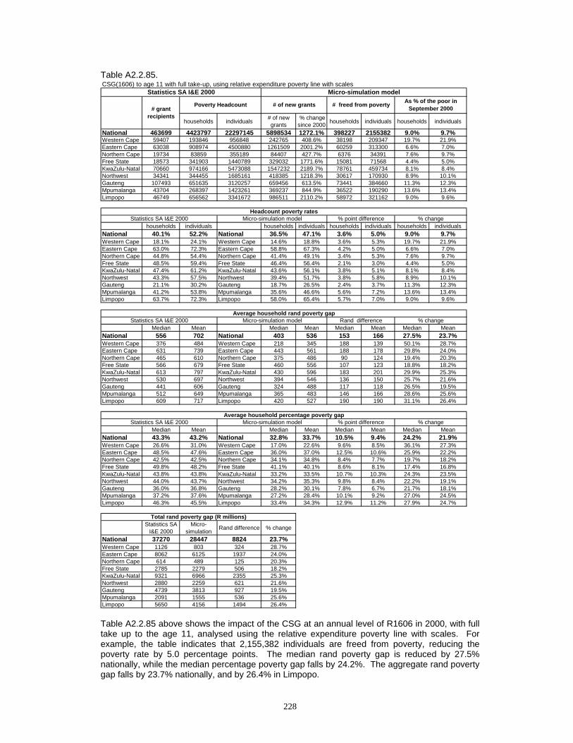
228
Table A2.2.85.
Table A2.2.85 above shows the impact of the CSG at an annual level of R1606 in 2000, with full take up to the age 11, analysed using the relative expenditure poverty line with scales. For example, the table indicates that 2,155,382 individuals are freed from poverty, reducing the poverty rate by 5.0 percentage points. The median rand poverty gap is reduced by 27.5% nationally, while the median percentage poverty gap falls by 24.2%. The aggregate rand poverty gap falls by 23.7% nationally, and by 26.4% in Limpopo.
CSG(1606) to age 11 with full take-up, using relative expenditure poverty line with scales
households individuals # of new grants
% change since 2000 households individuals households individuals
National 463699 4423797 22297145 5898534 1272.1% 398227 2155382 9.0% 9.7%Western Cape 59407 193846 956848 242765 408.6% 38198 209347 19.7% 21.9%Eastern Cape 63038 908974 4500880 1261509 2001.2% 60259 313300 6.6% 7.0%Northern Cape 19734 83859 355189 84407 427.7% 6376 34391 7.6% 9.7%Free State 18573 341903 1440789 329032 1771.6% 15081 71568 4.4% 5.0%KwaZulu-Natal 70660 974166 5473088 1547232 2189.7% 78761 459734 8.1% 8.4%Northwest 34341 344455 1685161 418385 1218.3% 30617 170930 8.9% 10.1%Gauteng 107493 651635 3120257 659456 613.5% 73441 384660 11.3% 12.3%Mpumalanga 43704 268397 1423261 369237 844.9% 36522 190290 13.6% 13.4%Limpopo 46749 656562 3341672 986511 2110.2% 58972 321162 9.0% 9.6%
households individuals households individuals households individuals households individualsNational 40.1% 52.2% National 36.5% 47.1% 3.6% 5.0% 9.0% 9.7%Western Cape 18.1% 24.1% Western Cape 14.6% 18.8% 3.6% 5.3% 19.7% 21.9%Eastern Cape 63.0% 72.3% Eastern Cape 58.8% 67.3% 4.2% 5.0% 6.6% 7.0%Northern Cape 44.8% 54.4% Northern Cape 41.4% 49.1% 3.4% 5.3% 7.6% 9.7%Free State 48.5% 59.4% Free State 46.4% 56.4% 2.1% 3.0% 4.4% 5.0%KwaZulu-Natal 47.4% 61.2% KwaZulu-Natal 43.6% 56.1% 3.8% 5.1% 8.1% 8.4%Northwest 43.3% 57.5% Northwest 39.4% 51.7% 3.8% 5.8% 8.9% 10.1%Gauteng 21.1% 30.2% Gauteng 18.7% 26.5% 2.4% 3.7% 11.3% 12.3%Mpumalanga 41.2% 53.8% Mpumalanga 35.6% 46.6% 5.6% 7.2% 13.6% 13.4%Limpopo 63.7% 72.3% Limpopo 58.0% 65.4% 5.7% 7.0% 9.0% 9.6%
Median Mean Median Mean Median Mean Median MeanNational 556 702 National 403 536 153 166 27.5% 23.7%Western Cape 376 484 Western Cape 218 345 188 139 50.1% 28.7%Eastern Cape 631 739 Eastern Cape 443 561 188 178 29.8% 24.0%Northern Cape 465 610 Northern Cape 375 486 90 124 19.4% 20.3%Free State 566 679 Free State 460 556 107 123 18.8% 18.2%KwaZulu-Natal 613 797 KwaZulu-Natal 430 596 183 201 29.9% 25.3%Northwest 530 697 Northwest 394 546 136 150 25.7% 21.6%Gauteng 441 606 Gauteng 324 488 117 118 26.5% 19.5%Mpumalanga 512 649 Mpumalanga 365 483 146 166 28.6% 25.6%Limpopo 609 717 Limpopo 420 527 190 190 31.1% 26.4%
Median Mean Median Mean Median Mean Median MeanNational 43.3% 43.2% National 32.8% 33.7% 10.5% 9.4% 24.2% 21.9%Western Cape 26.6% 31.0% Western Cape 17.0% 22.6% 9.6% 8.5% 36.1% 27.3%Eastern Cape 48.5% 47.6% Eastern Cape 36.0% 37.0% 12.5% 10.6% 25.9% 22.2%Northern Cape 42.5% 42.5% Northern Cape 34.1% 34.8% 8.4% 7.7% 19.7% 18.2%Free State 49.8% 48.2% Free State 41.1% 40.1% 8.6% 8.1% 17.4% 16.8%KwaZulu-Natal 43.8% 43.8% KwaZulu-Natal 33.2% 33.5% 10.7% 10.3% 24.3% 23.5%Northwest 44.0% 43.7% Northwest 34.2% 35.3% 9.8% 8.4% 22.2% 19.1%Gauteng 36.0% 36.8% Gauteng 28.2% 30.1% 7.8% 6.7% 21.7% 18.1%Mpumalanga 37.2% 37.6% Mpumalanga 27.2% 28.4% 10.1% 9.2% 27.0% 24.5%Limpopo 46.3% 45.5% Limpopo 33.4% 34.3% 12.9% 11.2% 27.9% 24.7%
Statistics SA I&E 2000
Micro-simulation Rand difference % change
National 37270 28447 8824 23.7%Western Cape 1126 803 324 28.7%Eastern Cape 8062 6125 1937 24.0%Northern Cape 614 489 125 20.3%Free State 2785 2279 506 18.2%KwaZulu-Natal 9321 6966 2355 25.3%Northwest 2880 2259 621 21.6%Gauteng 4739 3813 927 19.5%Mpumalanga 2091 1555 536 25.6%Limpopo 5650 4156 1494 26.4%
Total rand poverty gap (R millions)
Statistics SA I&E 2000 Micro-simulation model
Micro-simulation modelStatistics SA I&E 2000
Poverty Headcount# grant
recipients
% point differenceAverage household percentage poverty gap
Average household rand poverty gap% change
% changeMicro-simulation model
% change
Headcount poverty rates
# of new grants # freed from poverty As % of the poor in September 2000
Statistics SA I&E 2000 % point difference
Statistics SA I&E 2000 Micro-simulation model Rand difference

229
Table A2.2.86.
Table A2.2.86 above shows the impact of the CSG at an annual level of R1606 in 2000, with full take up to the age 14, analysed using the relative expenditure poverty line with scales. For example, the table indicates that 2,940,818 individuals are freed from poverty, reducing the poverty rate by 6.9 percentage points. The median rand poverty gap is reduced by 35.1% nationally, while the median percentage poverty gap falls by 31.3%. The aggregate rand poverty gap falls by 30.5% nationally, and by 34.2% in Limpopo.
CSG(1606) to age 14 with full take-up, using relative expenditure poverty line with scales
households individuals # of new grants
% change since 2000 households individuals households individuals
National 463699 4423797 22297145 7704751 1661.6% 543587 2940818 12.3% 13.2%Western Cape 59407 193846 956848 303305 510.6% 45377 252223 23.4% 26.4%Eastern Cape 63038 908974 4500880 1683786 2671.1% 89754 476052 9.9% 10.6%Northern Cape 19734 83859 355189 107004 542.2% 7932 41341 9.5% 11.6%Free State 18573 341903 1440789 430996 2320.6% 22650 107287 6.6% 7.4%KwaZulu-Natal 70660 974166 5473088 2000256 2830.8% 115315 656362 11.8% 12.0%Northwest 34341 344455 1685161 551438 1605.8% 38351 212575 11.1% 12.6%Gauteng 107493 651635 3120257 843083 784.3% 88676 475847 13.6% 15.3%Mpumalanga 43704 268397 1423261 488058 1116.7% 51704 273286 19.3% 19.2%Limpopo 46749 656562 3341672 1296825 2774.0% 83828 445845 12.8% 13.3%
households individuals households individuals households individuals households individualsNational 40.1% 52.2% National 35.2% 45.3% 4.9% 6.9% 12.3% 13.2%Western Cape 18.1% 24.1% Western Cape 13.9% 17.8% 4.2% 6.4% 23.4% 26.4%Eastern Cape 63.0% 72.3% Eastern Cape 56.7% 64.6% 6.2% 7.6% 9.9% 10.6%Northern Cape 44.8% 54.4% Northern Cape 40.6% 48.1% 4.2% 6.3% 9.5% 11.6%Free State 48.5% 59.4% Free State 45.3% 55.0% 3.2% 4.4% 6.6% 7.4%KwaZulu-Natal 47.4% 61.2% KwaZulu-Natal 41.8% 53.9% 5.6% 7.3% 11.8% 12.0%Northwest 43.3% 57.5% Northwest 38.5% 50.2% 4.8% 7.3% 11.1% 12.6%Gauteng 21.1% 30.2% Gauteng 18.2% 25.6% 2.9% 4.6% 13.6% 15.3%Mpumalanga 41.2% 53.8% Mpumalanga 33.2% 43.5% 7.9% 10.3% 19.3% 19.2%Limpopo 63.7% 72.3% Limpopo 55.6% 62.7% 8.1% 9.7% 12.8% 13.3%
Median Mean Median Mean Median Mean Median MeanNational 556 702 National 361 488 195 214 35.1% 30.5%Western Cape 376 484 Western Cape 193 315 242 169 64.4% 34.9%Eastern Cape 631 739 Eastern Cape 389 507 242 232 38.3% 31.5%Northern Cape 465 610 Northern Cape 347 455 118 155 25.4% 25.4%Free State 566 679 Free State 437 519 130 160 22.9% 23.6%KwaZulu-Natal 613 797 KwaZulu-Natal 390 541 224 256 36.5% 32.1%Northwest 530 697 Northwest 374 501 155 196 29.3% 28.1%Gauteng 441 606 Gauteng 300 455 142 151 32.1% 24.9%Mpumalanga 512 649 Mpumalanga 315 435 197 214 38.5% 33.0%Limpopo 609 717 Limpopo 361 472 248 245 40.7% 34.2%
Median Mean Median Mean Median Mean Median MeanNational 43.3% 43.2% National 29.7% 31.0% 13.5% 12.2% 31.3% 28.2%Western Cape 26.6% 31.0% Western Cape 15.3% 20.8% 11.3% 10.2% 42.5% 32.8%Eastern Cape 48.5% 47.6% Eastern Cape 32.4% 33.7% 16.1% 13.9% 33.1% 29.2%Northern Cape 42.5% 42.5% Northern Cape 32.6% 32.9% 9.8% 9.6% 23.2% 22.6%Free State 49.8% 48.2% Free State 38.1% 37.7% 11.7% 10.5% 23.6% 21.7%KwaZulu-Natal 43.8% 43.8% KwaZulu-Natal 29.7% 30.6% 14.1% 13.1% 32.3% 30.0%Northwest 44.0% 43.7% Northwest 31.4% 32.8% 12.6% 11.0% 28.6% 25.1%Gauteng 36.0% 36.8% Gauteng 25.9% 28.5% 10.0% 8.3% 27.9% 22.6%Mpumalanga 37.2% 37.6% Mpumalanga 24.4% 25.7% 12.8% 11.9% 34.3% 31.6%Limpopo 46.3% 45.5% Limpopo 29.4% 30.9% 16.8% 14.7% 36.4% 32.2%
Statistics SA I&E 2000
Micro-simulation Rand difference % change
National 37270 25920 11350 30.5%Western Cape 1126 734 393 34.9%Eastern Cape 8062 5526 2536 31.5%Northern Cape 614 458 156 25.4%Free State 2785 2128 657 23.6%KwaZulu-Natal 9321 6324 2996 32.1%Northwest 2880 2070 810 28.1%Gauteng 4739 3561 1178 24.9%Mpumalanga 2091 1401 690 33.0%Limpopo 5650 3716 1933 34.2%
Total rand poverty gap (R millions)
Statistics SA I&E 2000 Micro-simulation model
Micro-simulation modelStatistics SA I&E 2000
Poverty Headcount# grant
recipients
% point differenceAverage household percentage poverty gap
Average household rand poverty gap% change
% changeMicro-simulation model
% change
Headcount poverty rates
# of new grants # freed from poverty As % of the poor in September 2000
Statistics SA I&E 2000 % point difference
Statistics SA I&E 2000 Micro-simulation model Rand difference

230
Table A2.2.87.
Table A2.2.87 above shows the impact of the CSG at an annual level of R1606 in 2000, with full take up to the age 16, analysed using the relative expenditure poverty line with scales. For example, the table indicates that 3,495,288 individuals are freed from poverty, reducing the poverty rate by 8.2 percentage points. The median rand poverty gap is reduced by 40.5% nationally, while the median percentage poverty gap falls by 37.1%. The aggregate rand poverty gap falls by 34.8% nationally, and by 38.9% in Limpopo.
CSG(1606) to age 16 with full take-up, using relative expenditure poverty line with scales
households individuals # of new grants
% change since 2000 households individuals households individuals
National 463699 4423797 22297145 8908343 1921.1% 643609 3495288 14.5% 15.7%Western Cape 59407 193846 956848 352077 592.7% 55207 311685 28.5% 32.6%Eastern Cape 63038 908974 4500880 1957760 3105.7% 112204 594895 12.3% 13.2%Northern Cape 19734 83859 355189 122032 618.4% 9612 49217 11.5% 13.9%Free State 18573 341903 1440789 503531 2711.1% 28017 130331 8.2% 9.0%KwaZulu-Natal 70660 974166 5473088 2310804 3270.3% 134076 752627 13.8% 13.8%Northwest 34341 344455 1685161 639862 1863.3% 48911 280895 14.2% 16.7%Gauteng 107493 651635 3120257 955564 889.0% 96578 532518 14.8% 17.1%Mpumalanga 43704 268397 1423261 568445 1300.7% 57336 303829 21.4% 21.3%Limpopo 46749 656562 3341672 1498268 3204.9% 101668 539291 15.5% 16.1%
households individuals households individuals households individuals households individualsNational 40.1% 52.2% National 34.3% 44.0% 5.8% 8.2% 14.5% 15.7%Western Cape 18.1% 24.1% Western Cape 13.0% 16.3% 5.2% 7.9% 28.5% 32.6%Eastern Cape 63.0% 72.3% Eastern Cape 55.2% 62.7% 7.8% 9.6% 12.3% 13.2%Northern Cape 44.8% 54.4% Northern Cape 39.7% 46.9% 5.1% 7.5% 11.5% 13.9%Free State 48.5% 59.4% Free State 44.6% 54.0% 4.0% 5.4% 8.2% 9.0%KwaZulu-Natal 47.4% 61.2% KwaZulu-Natal 40.9% 52.8% 6.5% 8.4% 13.8% 13.8%Northwest 43.3% 57.5% Northwest 37.1% 47.9% 6.1% 9.6% 14.2% 16.7%Gauteng 21.1% 30.2% Gauteng 18.0% 25.1% 3.1% 5.2% 14.8% 17.1%Mpumalanga 41.2% 53.8% Mpumalanga 32.4% 42.3% 8.8% 11.5% 21.4% 21.3%Limpopo 63.7% 72.3% Limpopo 53.8% 60.7% 9.9% 11.7% 15.5% 16.1%
Median Mean Median Mean Median Mean Median MeanNational 556 702 National 331 458 225 244 40.5% 34.8%Western Cape 376 484 Western Cape 171 293 273 192 72.5% 39.6%Eastern Cape 631 739 Eastern Cape 359 472 273 267 43.2% 36.2%Northern Cape 465 610 Northern Cape 338 435 127 175 27.3% 28.6%Free State 566 679 Free State 398 493 168 186 29.7% 27.4%KwaZulu-Natal 613 797 KwaZulu-Natal 350 504 263 294 42.9% 36.8%Northwest 530 697 Northwest 355 473 175 224 33.0% 32.1%Gauteng 441 606 Gauteng 288 436 153 170 34.7% 28.1%Mpumalanga 512 649 Mpumalanga 281 404 230 245 45.0% 37.8%Limpopo 609 717 Limpopo 322 438 287 279 47.2% 38.9%
Median Mean Median Mean Median Mean Median MeanNational 43.3% 43.2% National 27.2% 29.2% 16.0% 13.9% 37.1% 32.3%Western Cape 26.6% 31.0% Western Cape 13.2% 19.6% 13.4% 11.4% 50.3% 36.8%Eastern Cape 48.5% 47.6% Eastern Cape 29.9% 31.5% 18.6% 16.1% 38.4% 33.8%Northern Cape 42.5% 42.5% Northern Cape 31.7% 31.7% 10.8% 10.8% 25.4% 25.5%Free State 49.8% 48.2% Free State 36.2% 35.9% 13.6% 12.2% 27.2% 25.4%KwaZulu-Natal 43.8% 43.8% KwaZulu-Natal 26.8% 28.7% 17.0% 15.1% 38.8% 34.4%Northwest 44.0% 43.7% Northwest 29.5% 31.2% 14.5% 12.5% 33.0% 28.7%Gauteng 36.0% 36.8% Gauteng 25.1% 27.4% 10.8% 9.4% 30.2% 25.5%Mpumalanga 37.2% 37.6% Mpumalanga 21.9% 24.0% 15.3% 13.6% 41.1% 36.1%Limpopo 46.3% 45.5% Limpopo 26.1% 28.9% 20.2% 16.7% 43.6% 36.6%
Statistics SA I&E 2000
Micro-simulation Rand difference % change
National 37270 24295 12975 34.8%Western Cape 1126 681 446 39.6%Eastern Cape 8062 5146 2915 36.2%Northern Cape 614 438 176 28.6%Free State 2785 2021 764 27.4%KwaZulu-Natal 9321 5889 3431 36.8%Northwest 2880 1955 925 32.1%Gauteng 4739 3407 1333 28.1%Mpumalanga 2091 1301 790 37.8%Limpopo 5650 3454 2196 38.9%
Total rand poverty gap (R millions)
Statistics SA I&E 2000 Micro-simulation model
Micro-simulation modelStatistics SA I&E 2000
Poverty Headcount# grant
recipients
% point differenceAverage household percentage poverty gap
Average household rand poverty gap% change
% changeMicro-simulation model
% change
Headcount poverty rates
# of new grants # freed from poverty As % of the poor in September 2000
Statistics SA I&E 2000 % point difference
Statistics SA I&E 2000 Micro-simulation model Rand difference

231
Table A2.2.88.
Table A2.2.88 above shows the impact of the CSG at an annual level of R1606 in 2000, with full take up to the age 18, analysed using the relative expenditure poverty line with scales. For example, the table indicates that 4,048,927 individuals are freed from poverty, reducing the poverty rate by 9.5 percentage points. The median rand poverty gap is reduced by 45.0% nationally, while the median percentage poverty gap falls by 40.7%. The aggregate rand poverty gap falls by 38.7% nationally, and by 43.0% in Limpopo.
CSG(1606) to age 18 with full take-up, using relative expenditure poverty line with scales
households individuals # of new grants
% change since 2000 households individuals households individuals
National 463699 4423797 22297145 10004785 2157.6% 746192 4048927 16.9% 18.2%Western Cape 59407 193846 956848 394058 663.3% 59200 334112 30.5% 34.9%Eastern Cape 63038 908974 4500880 2207293 3501.5% 137764 722581 15.2% 16.1%Northern Cape 19734 83859 355189 135505 686.7% 10517 55269 12.5% 15.6%Free State 18573 341903 1440789 578117 3112.7% 33356 155957 9.8% 10.8%KwaZulu-Natal 70660 974166 5473088 2584348 3657.4% 159107 902921 16.3% 16.5%Northwest 34341 344455 1685161 712385 2074.4% 57071 324364 16.6% 19.2%Gauteng 107493 651635 3120257 1067394 993.0% 104878 570693 16.1% 18.3%Mpumalanga 43704 268397 1423261 646154 1478.5% 64527 340757 24.0% 23.9%Limpopo 46749 656562 3341672 1679531 3592.7% 119772 642273 18.2% 19.2%
households individuals households individuals households individuals households individualsNational 40.1% 52.2% National 33.4% 42.7% 6.8% 9.5% 16.9% 18.2%Western Cape 18.1% 24.1% Western Cape 12.6% 15.7% 5.5% 8.4% 30.5% 34.9%Eastern Cape 63.0% 72.3% Eastern Cape 53.4% 60.7% 9.5% 11.6% 15.2% 16.1%Northern Cape 44.8% 54.4% Northern Cape 39.2% 45.9% 5.6% 8.5% 12.5% 15.6%Free State 48.5% 59.4% Free State 43.8% 53.0% 4.7% 6.4% 9.8% 10.8%KwaZulu-Natal 47.4% 61.2% KwaZulu-Natal 39.7% 51.1% 7.7% 10.1% 16.3% 16.5%Northwest 43.3% 57.5% Northwest 36.1% 46.4% 7.2% 11.1% 16.6% 19.2%Gauteng 21.1% 30.2% Gauteng 17.7% 24.7% 3.4% 5.5% 16.1% 18.3%Mpumalanga 41.2% 53.8% Mpumalanga 31.3% 40.9% 9.9% 12.9% 24.0% 23.9%Limpopo 63.7% 72.3% Limpopo 52.1% 58.4% 11.6% 13.9% 18.2% 19.2%
Median Mean Median Mean Median Mean Median MeanNational 556 702 National 306 430 250 272 45.0% 38.7%Western Cape 376 484 Western Cape 137 273 297 211 78.9% 43.5%Eastern Cape 631 739 Eastern Cape 335 442 297 297 47.0% 40.2%Northern Cape 465 610 Northern Cape 322 418 143 192 30.7% 31.5%Free State 566 679 Free State 382 466 184 212 32.5% 31.3%KwaZulu-Natal 613 797 KwaZulu-Natal 326 472 287 325 46.8% 40.8%Northwest 530 697 Northwest 336 450 194 247 36.6% 35.4%Gauteng 441 606 Gauteng 279 417 162 189 36.7% 31.2%Mpumalanga 512 649 Mpumalanga 256 373 256 276 49.9% 42.5%Limpopo 609 717 Limpopo 297 409 312 308 51.2% 43.0%
Median Mean Median Mean Median Mean Median MeanNational 43.3% 43.2% National 25.7% 27.7% 17.6% 15.5% 40.7% 35.9%Western Cape 26.6% 31.0% Western Cape 12.2% 18.5% 14.4% 12.5% 54.1% 40.2%Eastern Cape 48.5% 47.6% Eastern Cape 28.4% 29.7% 20.1% 17.9% 41.5% 37.6%Northern Cape 42.5% 42.5% Northern Cape 30.8% 30.6% 11.7% 12.0% 27.5% 28.1%Free State 49.8% 48.2% Free State 34.2% 34.0% 15.5% 14.1% 31.2% 29.3%KwaZulu-Natal 43.8% 43.8% KwaZulu-Natal 25.5% 27.1% 18.3% 16.7% 41.8% 38.1%Northwest 44.0% 43.7% Northwest 27.8% 29.9% 16.2% 13.8% 36.7% 31.6%Gauteng 36.0% 36.8% Gauteng 24.3% 26.4% 11.7% 10.4% 32.4% 28.2%Mpumalanga 37.2% 37.6% Mpumalanga 20.4% 22.4% 16.8% 15.2% 45.1% 40.5%Limpopo 46.3% 45.5% Limpopo 24.3% 27.1% 22.0% 18.4% 47.5% 40.5%
Statistics SA I&E 2000
Micro-simulation Rand difference % change
National 37270 22852 14418 38.7%Western Cape 1126 636 490 43.5%Eastern Cape 8062 4820 3241 40.2%Northern Cape 614 420 193 31.5%Free State 2785 1914 871 31.3%KwaZulu-Natal 9321 5516 3805 40.8%Northwest 2880 1861 1019 35.4%Gauteng 4739 3259 1481 31.2%Mpumalanga 2091 1203 888 42.5%Limpopo 5650 3221 2429 43.0%
Total rand poverty gap (R millions)
Statistics SA I&E 2000 Micro-simulation model
Micro-simulation modelStatistics SA I&E 2000
Poverty Headcount# grant
recipients
% point differenceAverage household percentage poverty gap
Average household rand poverty gap% change
% changeMicro-simulation model
% change
Headcount poverty rates
# of new grants # freed from poverty As % of the poor in September 2000
Statistics SA I&E 2000 % point difference
Statistics SA I&E 2000 Micro-simulation model Rand difference

232
Table A2.2.89.
Table A2.2.89 above shows the impact of all grants with full take up, with the CSG at an annual level of R1200 in 2000, analysed using the relative expenditure poverty line with scales. For example, the table indicates that 3,386,274 individuals are freed from poverty, reducing the poverty rate by 7.9 percentage points. The median rand poverty gap is reduced by 40.2% nationally, while the median percentage poverty gap falls by 36.7%. The aggregate rand poverty gap falls by 33.5% nationally, and by 34.2% in Limpopo.
All grants with full take-up, using relative expenxiture poverty line with scales
households individuals # of new grants
% change since 2000 households individuals households individuals
National 2656508 4423797 22297145 8878404 334.2% 683579 3386274 15.5% 15.2%Western Cape 241897 193846 956848 386937 160.0% 48907 254792 25.2% 26.6%Eastern Cape 499290 908974 4500880 1909328 382.4% 136668 626181 15.0% 13.9%Northern Cape 69402 83859 355189 136214 196.3% 13652 65111 16.3% 18.3%Free State 131645 341903 1440789 507011 385.1% 35808 162739 10.5% 11.3%KwaZulu-Natal 522017 974166 5473088 2240055 429.1% 131876 687486 13.5% 12.6%Northwest 208084 344455 1685161 652478 313.6% 64098 321081 18.6% 19.1%Gauteng 471943 651635 3120257 1082832 229.4% 113493 573792 17.4% 18.4%Mpumalanga 161387 268397 1423261 553405 342.9% 52565 265423 19.6% 18.6%Limpopo 350843 656562 3341672 1410144 401.9% 86512 429669 13.2% 12.9%
households individuals households individuals households individuals households individualsNational 40.1% 52.2% National 33.9% 44.3% 6.2% 7.9% 15.5% 15.2%Western Cape 18.1% 24.1% Western Cape 13.6% 17.7% 4.6% 6.4% 25.2% 26.6%Eastern Cape 63.0% 72.3% Eastern Cape 53.5% 62.2% 9.5% 10.1% 15.0% 13.9%Northern Cape 44.8% 54.4% Northern Cape 37.5% 44.4% 7.3% 10.0% 16.3% 18.3%Free State 48.5% 59.4% Free State 43.5% 52.7% 5.1% 6.7% 10.5% 11.3%KwaZulu-Natal 47.4% 61.2% KwaZulu-Natal 41.0% 53.5% 6.4% 7.7% 13.5% 12.6%Northwest 43.3% 57.5% Northwest 35.2% 46.5% 8.1% 11.0% 18.6% 19.1%Gauteng 21.1% 30.2% Gauteng 17.4% 24.7% 3.7% 5.6% 17.4% 18.4%Mpumalanga 41.2% 53.8% Mpumalanga 33.1% 43.8% 8.1% 10.0% 19.6% 18.6%Limpopo 63.7% 72.3% Limpopo 55.3% 63.0% 8.4% 9.3% 13.2% 12.9%
Median Mean Median Mean Median Mean Median MeanNational 556 702 National 333 467 224 235 40.2% 33.5%Western Cape 376 484 Western Cape 171 309 274 176 72.9% 36.3%Eastern Cape 631 739 Eastern Cape 357 480 274 259 43.4% 35.1%Northern Cape 465 610 Northern Cape 295 411 171 199 36.7% 32.7%Free State 566 679 Free State 398 493 168 186 29.8% 27.4%KwaZulu-Natal 613 797 KwaZulu-Natal 367 527 246 270 40.2% 33.8%Northwest 530 697 Northwest 324 452 205 245 38.8% 35.2%Gauteng 441 606 Gauteng 274 422 167 184 37.9% 30.4%Mpumalanga 512 649 Mpumalanga 290 420 222 229 43.3% 35.3%Limpopo 609 717 Limpopo 366 472 244 245 40.0% 34.2%
Median Mean Median Mean Median Mean Median MeanNational 43.3% 43.2% National 27.4% 29.5% 15.9% 13.7% 36.7% 31.8%Western Cape 26.6% 31.0% Western Cape 13.4% 20.0% 13.2% 11.0% 49.6% 35.4%Eastern Cape 48.5% 47.6% Eastern Cape 30.9% 31.5% 17.6% 16.1% 36.2% 33.7%Northern Cape 42.5% 42.5% Northern Cape 28.3% 29.9% 14.2% 12.7% 33.5% 29.8%Free State 49.8% 48.2% Free State 37.2% 36.0% 12.6% 12.1% 25.2% 25.2%KwaZulu-Natal 43.8% 43.8% KwaZulu-Natal 28.0% 29.5% 15.8% 14.3% 36.0% 32.7%Northwest 44.0% 43.7% Northwest 26.8% 29.5% 17.2% 14.2% 39.2% 32.5%Gauteng 36.0% 36.8% Gauteng 23.4% 26.5% 12.6% 10.3% 35.0% 27.9%Mpumalanga 37.2% 37.6% Mpumalanga 22.8% 24.9% 14.4% 12.7% 38.7% 33.8%Limpopo 46.3% 45.5% Limpopo 28.6% 30.5% 17.7% 15.0% 38.2% 32.9%
Statistics SA I&E 2000
Micro-simulation Rand difference % change
National 37270 24786 12484 33.5%Western Cape 1126 718 408 36.3%Eastern Cape 8062 5232 2830 35.1%Northern Cape 614 413 201 32.7%Free State 2785 2021 764 27.4%KwaZulu-Natal 9321 6166 3155 33.8%Northwest 2880 1867 1014 35.2%Gauteng 4739 3298 1442 30.4%Mpumalanga 2091 1352 739 35.3%Limpopo 5650 3717 1933 34.2%
Total rand poverty gap (R millions)
Statistics SA I&E 2000 Micro-simulation model
Micro-simulation modelStatistics SA I&E 2000
Poverty Headcount# grant
recipients
% point differenceAverage household percentage poverty gap
Average household rand poverty gap% change
% changeMicro-simulation model
% change
Headcount poverty rates
# of new grants # freed from poverty As % of the poor in September 2000
Statistics SA I&E 2000 % point difference
Statistics SA I&E 2000 Micro-simulation model Rand difference
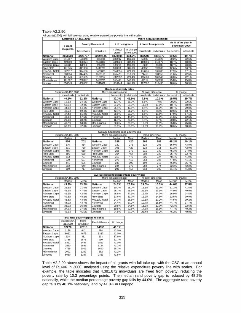
233
Table A2.2.90.
Table A2.2.90 above shows the impact of all grants with full take up, with the CSG at an annual level of R1606 in 2000, analysed using the relative expenditure poverty line with scales. For example, the table indicates that 4,381,872 individuals are freed from poverty, reducing the poverty rate by 10.3 percentage points. The median rand poverty gap is reduced by 48.2% nationally, while the median percentage poverty gap falls by 44.0%. The aggregate rand poverty gap falls by 40.1% nationally, and by 41.8% in Limpopo.
All grants(1606) with full take-up, using relative expenxiture poverty line with scales
households individuals # of new grants
% change since 2000 households individuals households individuals
National 2656508 4423797 22297145 8878404 334.2% 862706 4381872 19.5% 19.7%Western Cape 241897 193846 956848 386937 160.0% 58599 312025 30.2% 32.6%Eastern Cape 499290 908974 4500880 1909328 382.4% 169596 810579 18.7% 18.0%Northern Cape 69402 83859 355189 136214 196.3% 15698 73878 18.7% 20.8%Free State 131645 341903 1440789 507011 385.1% 42950 197832 12.6% 13.7%KwaZulu-Natal 522017 974166 5473088 2240055 429.1% 174736 937283 17.9% 17.1%Northwest 208084 344455 1685161 652478 313.6% 74418 381555 21.6% 22.6%Gauteng 471943 651635 3120257 1082832 229.4% 135588 689346 20.8% 22.1%Mpumalanga 161387 268397 1423261 553405 342.9% 69119 366939 25.8% 25.8%Limpopo 350843 656562 3341672 1410144 401.9% 122002 612435 18.6% 18.3%
households individuals households individuals households individuals households individualsNational 40.1% 52.2% National 32.3% 41.9% 7.8% 10.3% 19.5% 19.7%Western Cape 18.1% 24.1% Western Cape 12.7% 16.3% 5.5% 7.9% 30.2% 32.6%Eastern Cape 63.0% 72.3% Eastern Cape 51.2% 59.3% 11.7% 13.0% 18.7% 18.0%Northern Cape 44.8% 54.4% Northern Cape 36.4% 43.1% 8.4% 11.3% 18.7% 20.8%Free State 48.5% 59.4% Free State 42.4% 51.2% 6.1% 8.2% 12.6% 13.7%KwaZulu-Natal 47.4% 61.2% KwaZulu-Natal 38.9% 50.7% 8.5% 10.5% 17.9% 17.1%Northwest 43.3% 57.5% Northwest 33.9% 44.5% 9.4% 13.0% 21.6% 22.6%Gauteng 21.1% 30.2% Gauteng 16.7% 23.6% 4.4% 6.7% 20.8% 22.1%Mpumalanga 41.2% 53.8% Mpumalanga 30.6% 39.9% 10.6% 13.9% 25.8% 25.8%Limpopo 63.7% 72.3% Limpopo 51.9% 59.1% 11.8% 13.3% 18.6% 18.3%
Median Mean Median Mean Median Mean Median MeanNational 556 702 National 288 420 268 282 48.2% 40.1%Western Cape 376 484 Western Cape 130 276 323 208 85.9% 43.0%Eastern Cape 631 739 Eastern Cape 308 429 323 311 51.2% 42.0%Northern Cape 465 610 Northern Cape 255 379 211 232 45.3% 37.9%Free State 566 679 Free State 364 457 202 222 35.7% 32.7%KwaZulu-Natal 613 797 KwaZulu-Natal 318 470 295 327 48.1% 41.0%Northwest 530 697 Northwest 276 410 253 286 47.8% 41.1%Gauteng 441 606 Gauteng 243 390 199 216 45.0% 35.7%Mpumalanga 512 649 Mpumalanga 244 375 268 274 52.3% 42.2%Limpopo 609 717 Limpopo 296 417 313 300 51.4% 41.8%
Median Mean Median Mean Median Mean Median MeanNational 43.3% 43.2% National 24.2% 26.8% 19.0% 16.3% 44.0% 37.8%Western Cape 26.6% 31.0% Western Cape 10.3% 18.0% 16.3% 13.0% 61.2% 41.8%Eastern Cape 48.5% 47.6% Eastern Cape 26.7% 28.5% 21.8% 19.1% 44.9% 40.0%Northern Cape 42.5% 42.5% Northern Cape 26.8% 27.9% 15.7% 14.7% 36.9% 34.5%Free State 49.8% 48.2% Free State 33.6% 33.7% 16.2% 14.5% 32.5% 30.0%KwaZulu-Natal 43.8% 43.8% KwaZulu-Natal 24.3% 26.6% 19.5% 17.2% 44.5% 39.2%Northwest 44.0% 43.7% Northwest 24.4% 27.2% 19.7% 16.5% 44.7% 37.7%Gauteng 36.0% 36.8% Gauteng 20.8% 24.8% 15.2% 12.0% 42.3% 32.6%Mpumalanga 37.2% 37.6% Mpumalanga 19.5% 22.5% 17.8% 15.1% 47.7% 40.2%Limpopo 46.3% 45.5% Limpopo 24.8% 27.3% 21.4% 18.2% 46.3% 40.0%
Statistics SA I&E 2000
Micro-simulation Rand difference % change
National 37270 22315 14955 40.1%Western Cape 1126 642 484 43.0%Eastern Cape 8062 4675 3387 42.0%Northern Cape 614 381 233 37.9%Free State 2785 1875 910 32.7%KwaZulu-Natal 9321 5497 3823 41.0%Northwest 2880 1696 1184 41.1%Gauteng 4739 3049 1690 35.7%Mpumalanga 2091 1209 882 42.2%Limpopo 5650 3287 2363 41.8%
Total rand poverty gap (R millions)
Statistics SA I&E 2000 Micro-simulation model
Micro-simulation modelStatistics SA I&E 2000
Poverty Headcount# grant
recipients
% point differenceAverage household percentage poverty gap
Average household rand poverty gap% change
% changeMicro-simulation model
% change
Headcount poverty rates
# of new grants # freed from poverty As % of the poor in September 2000
Statistics SA I&E 2000 % point difference
Statistics SA I&E 2000 Micro-simulation model Rand difference
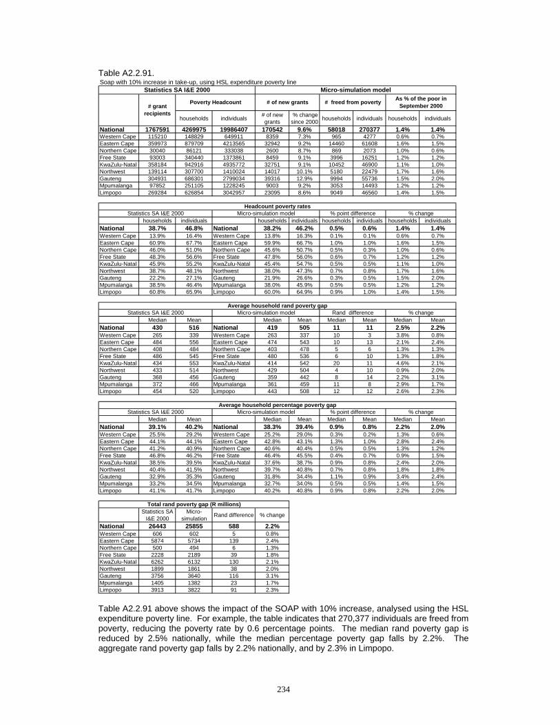
234
Table A2.2.91.
Table A2.2.91 above shows the impact of the SOAP with 10% increase, analysed using the HSL expenditure poverty line. For example, the table indicates that 270,377 individuals are freed from poverty, reducing the poverty rate by 0.6 percentage points. The median rand poverty gap is reduced by 2.5% nationally, while the median percentage poverty gap falls by 2.2%. The aggregate rand poverty gap falls by 2.2% nationally, and by 2.3% in Limpopo.
Soap with 10% increase in take-up, using HSL expenditure poverty line
households individuals # of new grants
% change since 2000 households individuals households individuals
National 1767591 4269975 19986407 170542 9.6% 58018 270377 1.4% 1.4%Western Cape 115210 148829 649911 8359 7.3% 965 4277 0.6% 0.7%Eastern Cape 359973 879709 4213565 32942 9.2% 14460 61608 1.6% 1.5%Northern Cape 30040 86121 333038 2600 8.7% 869 2073 1.0% 0.6%Free State 93003 340440 1373861 8459 9.1% 3996 16251 1.2% 1.2%KwaZulu-Natal 358184 942916 4935772 32751 9.1% 10452 46900 1.1% 1.0%Northwest 139114 307700 1410024 14017 10.1% 5180 22479 1.7% 1.6%Gauteng 304931 686301 2799034 39316 12.9% 9994 55736 1.5% 2.0%Mpumalanga 97852 251105 1228245 9003 9.2% 3053 14493 1.2% 1.2%Limpopo 269284 626854 3042957 23095 8.6% 9049 46560 1.4% 1.5%
households individuals households individuals households individuals households individualsNational 38.7% 46.8% National 38.2% 46.2% 0.5% 0.6% 1.4% 1.4%Western Cape 13.9% 16.4% Western Cape 13.8% 16.3% 0.1% 0.1% 0.6% 0.7%Eastern Cape 60.9% 67.7% Eastern Cape 59.9% 66.7% 1.0% 1.0% 1.6% 1.5%Northern Cape 46.0% 51.0% Northern Cape 45.6% 50.7% 0.5% 0.3% 1.0% 0.6%Free State 48.3% 56.6% Free State 47.8% 56.0% 0.6% 0.7% 1.2% 1.2%KwaZulu-Natal 45.9% 55.2% KwaZulu-Natal 45.4% 54.7% 0.5% 0.5% 1.1% 1.0%Northwest 38.7% 48.1% Northwest 38.0% 47.3% 0.7% 0.8% 1.7% 1.6%Gauteng 22.2% 27.1% Gauteng 21.9% 26.6% 0.3% 0.5% 1.5% 2.0%Mpumalanga 38.5% 46.4% Mpumalanga 38.0% 45.9% 0.5% 0.5% 1.2% 1.2%Limpopo 60.8% 65.9% Limpopo 60.0% 64.9% 0.9% 1.0% 1.4% 1.5%
Median Mean Median Mean Median Mean Median MeanNational 430 516 National 419 505 11 11 2.5% 2.2%Western Cape 265 339 Western Cape 263 337 10 3 3.8% 0.8%Eastern Cape 484 556 Eastern Cape 474 543 10 13 2.1% 2.4%Northern Cape 408 484 Northern Cape 403 478 5 6 1.3% 1.3%Free State 486 545 Free State 480 536 6 10 1.3% 1.8%KwaZulu-Natal 434 553 KwaZulu-Natal 414 542 20 11 4.6% 2.1%Northwest 433 514 Northwest 429 504 4 10 0.9% 2.0%Gauteng 368 456 Gauteng 359 442 8 14 2.2% 3.1%Mpumalanga 372 466 Mpumalanga 361 459 11 8 2.9% 1.7%Limpopo 454 520 Limpopo 443 508 12 12 2.6% 2.3%
Median Mean Median Mean Median Mean Median MeanNational 39.1% 40.2% National 38.3% 39.4% 0.9% 0.8% 2.2% 2.0%Western Cape 25.5% 29.2% Western Cape 25.2% 29.0% 0.3% 0.2% 1.3% 0.6%Eastern Cape 44.1% 44.1% Eastern Cape 42.8% 43.1% 1.3% 1.0% 2.8% 2.4%Northern Cape 41.2% 40.9% Northern Cape 40.6% 40.4% 0.5% 0.5% 1.3% 1.2%Free State 46.8% 46.2% Free State 46.4% 45.5% 0.4% 0.7% 0.9% 1.5%KwaZulu-Natal 38.5% 39.5% KwaZulu-Natal 37.6% 38.7% 0.9% 0.8% 2.4% 2.0%Northwest 40.4% 41.5% Northwest 39.7% 40.8% 0.7% 0.8% 1.8% 1.8%Gauteng 32.9% 35.3% Gauteng 31.8% 34.4% 1.1% 0.9% 3.4% 2.4%Mpumalanga 33.2% 34.5% Mpumalanga 32.7% 34.0% 0.5% 0.5% 1.4% 1.5%Limpopo 41.1% 41.7% Limpopo 40.2% 40.8% 0.9% 0.8% 2.2% 2.0%
Statistics SA I&E 2000
Micro-simulation Rand difference % change
National 26443 25855 588 2.2%Western Cape 606 602 5 0.8%Eastern Cape 5874 5734 139 2.4%Northern Cape 500 494 6 1.3%Free State 2228 2189 39 1.8%KwaZulu-Natal 6262 6132 130 2.1%Northwest 1899 1861 38 2.0%Gauteng 3756 3640 116 3.1%Mpumalanga 1405 1382 23 1.7%Limpopo 3913 3822 91 2.3%
% change
Headcount poverty rates
# of new grants # freed from poverty As % of the poor in September 2000
Statistics SA I&E 2000 % point difference
Statistics SA I&E 2000 Micro-simulation model Rand differenceAverage household rand poverty gap
% change
% changeMicro-simulation model
Total rand poverty gap (R millions)
Statistics SA I&E 2000 Micro-simulation model
Micro-simulation modelStatistics SA I&E 2000
Poverty Headcount# grant
recipients
% point differenceAverage household percentage poverty gap
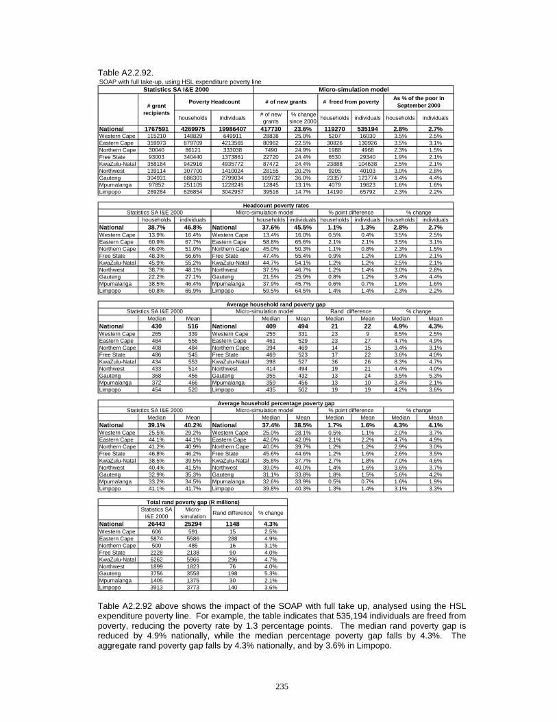
235
Table A2.2.92.
Table A2.2.92 above shows the impact of the SOAP with full take up, analysed using the HSL expenditure poverty line. For example, the table indicates that 535,194 individuals are freed from poverty, reducing the poverty rate by 1.3 percentage points. The median rand poverty gap is reduced by 4.9% nationally, while the median percentage poverty gap falls by 4.3%. The aggregate rand poverty gap falls by 4.3% nationally, and by 3.6% in Limpopo.
SOAP with full take-up, using HSL expenditure poverty line
households individuals # of new grants
% change since 2000 households individuals households individuals
National 1767591 4269975 19986407 417730 23.6% 119270 535194 2.8% 2.7%Western Cape 115210 148829 649911 28838 25.0% 5207 16030 3.5% 2.5%Eastern Cape 359973 879709 4213565 80962 22.5% 30826 130926 3.5% 3.1%Northern Cape 30040 86121 333038 7490 24.9% 1988 4968 2.3% 1.5%Free State 93003 340440 1373861 22720 24.4% 6530 29340 1.9% 2.1%KwaZulu-Natal 358184 942916 4935772 87472 24.4% 23888 104638 2.5% 2.1%Northwest 139114 307700 1410024 28155 20.2% 9205 40103 3.0% 2.8%Gauteng 304931 686301 2799034 109732 36.0% 23357 123774 3.4% 4.4%Mpumalanga 97852 251105 1228245 12845 13.1% 4079 19623 1.6% 1.6%Limpopo 269284 626854 3042957 39516 14.7% 14190 65792 2.3% 2.2%
households individuals households individuals households individuals households individualsNational 38.7% 46.8% National 37.6% 45.5% 1.1% 1.3% 2.8% 2.7%Western Cape 13.9% 16.4% Western Cape 13.4% 16.0% 0.5% 0.4% 3.5% 2.5%Eastern Cape 60.9% 67.7% Eastern Cape 58.8% 65.6% 2.1% 2.1% 3.5% 3.1%Northern Cape 46.0% 51.0% Northern Cape 45.0% 50.3% 1.1% 0.8% 2.3% 1.5%Free State 48.3% 56.6% Free State 47.4% 55.4% 0.9% 1.2% 1.9% 2.1%KwaZulu-Natal 45.9% 55.2% KwaZulu-Natal 44.7% 54.1% 1.2% 1.2% 2.5% 2.1%Northwest 38.7% 48.1% Northwest 37.5% 46.7% 1.2% 1.4% 3.0% 2.8%Gauteng 22.2% 27.1% Gauteng 21.5% 25.9% 0.8% 1.2% 3.4% 4.4%Mpumalanga 38.5% 46.4% Mpumalanga 37.9% 45.7% 0.6% 0.7% 1.6% 1.6%Limpopo 60.8% 65.9% Limpopo 59.5% 64.5% 1.4% 1.4% 2.3% 2.2%
Median Mean Median Mean Median Mean Median MeanNational 430 516 National 409 494 21 22 4.9% 4.3%Western Cape 265 339 Western Cape 255 331 23 9 8.5% 2.5%Eastern Cape 484 556 Eastern Cape 461 529 23 27 4.7% 4.9%Northern Cape 408 484 Northern Cape 394 469 14 15 3.4% 3.1%Free State 486 545 Free State 469 523 17 22 3.6% 4.0%KwaZulu-Natal 434 553 KwaZulu-Natal 398 527 36 26 8.3% 4.7%Northwest 433 514 Northwest 414 494 19 21 4.4% 4.0%Gauteng 368 456 Gauteng 355 432 13 24 3.5% 5.3%Mpumalanga 372 466 Mpumalanga 359 456 13 10 3.4% 2.1%Limpopo 454 520 Limpopo 435 502 19 19 4.2% 3.6%
Median Mean Median Mean Median Mean Median MeanNational 39.1% 40.2% National 37.4% 38.5% 1.7% 1.6% 4.3% 4.1%Western Cape 25.5% 29.2% Western Cape 25.0% 28.1% 0.5% 1.1% 2.0% 3.7%Eastern Cape 44.1% 44.1% Eastern Cape 42.0% 42.0% 2.1% 2.2% 4.7% 4.9%Northern Cape 41.2% 40.9% Northern Cape 40.0% 39.7% 1.2% 1.2% 2.9% 3.0%Free State 46.8% 46.2% Free State 45.6% 44.6% 1.2% 1.6% 2.6% 3.5%KwaZulu-Natal 38.5% 39.5% KwaZulu-Natal 35.8% 37.7% 2.7% 1.8% 7.0% 4.6%Northwest 40.4% 41.5% Northwest 39.0% 40.0% 1.4% 1.6% 3.6% 3.7%Gauteng 32.9% 35.3% Gauteng 31.1% 33.8% 1.8% 1.5% 5.6% 4.2%Mpumalanga 33.2% 34.5% Mpumalanga 32.6% 33.9% 0.5% 0.7% 1.6% 1.9%Limpopo 41.1% 41.7% Limpopo 39.8% 40.3% 1.3% 1.4% 3.1% 3.3%
Statistics SA I&E 2000
Micro-simulation Rand difference % change
National 26443 25294 1148 4.3%Western Cape 606 591 15 2.5%Eastern Cape 5874 5586 288 4.9%Northern Cape 500 485 16 3.1%Free State 2228 2138 90 4.0%KwaZulu-Natal 6262 5966 296 4.7%Northwest 1899 1823 76 4.0%Gauteng 3756 3558 198 5.3%Mpumalanga 1405 1375 30 2.1%Limpopo 3913 3773 140 3.6%
% change
Headcount poverty rates
# of new grants # freed from poverty As % of the poor in September 2000
Statistics SA I&E 2000 % point difference
Statistics SA I&E 2000 Micro-simulation model Rand differenceAverage household rand poverty gap
% change
% changeMicro-simulation model
Total rand poverty gap (R millions)
Statistics SA I&E 2000 Micro-simulation model
Micro-simulation modelStatistics SA I&E 2000
Poverty Headcount# grant
recipients
% point differenceAverage household percentage poverty gap
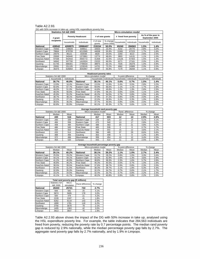
236
Table A2.2.93.
Table A2.2.93 above shows the impact of the DG with 50% increase in take up, analysed using the HSL expenditure poverty line. For example, the table indicates that 284,563 individuals are freed from poverty, reducing the poverty rate by 0.7 percentage points. The median rand poverty gap is reduced by 2.9% nationally, while the median percentage poverty gap falls by 2.7%. The aggregate rand poverty gap falls by 2.7% nationally, and by 1.9% in Limpopo.
DG with 50% increase in take-up, using HSL expenditure poverty line
households individuals # of new grants
% change since 2000 households individuals households individuals
National 438542 4269975 19986407 219154 50.0% 65240 284563 1.5% 1.4%Western Cape 70442 148829 649911 16503 23.4% 4142 20770 2.8% 3.2%Eastern Cape 78664 879709 4213565 44008 55.9% 15381 67223 1.7% 1.6%Northern Cape 20076 86121 333038 6828 34.0% 2260 8213 2.6% 2.5%Free State 20069 340440 1373861 13774 68.6% 3893 14131 1.1% 1.0%KwaZulu-Natal 97038 942916 4935772 41358 42.6% 14126 67403 1.5% 1.4%Northwest 34942 307700 1410024 23220 66.5% 6271 27161 2.0% 1.9%Gauteng 61745 686301 2799034 38975 63.1% 7026 26379 1.0% 0.9%Mpumalanga 20091 251105 1228245 14701 73.2% 4962 24989 2.0% 2.0%Limpopo 35475 626854 3042957 19787 55.8% 7179 28294 1.1% 0.9%
households individuals households individuals households individuals households individualsNational 38.7% 46.8% National 38.1% 46.1% 0.6% 0.7% 1.5% 1.4%Western Cape 13.9% 16.4% Western Cape 13.5% 15.9% 0.4% 0.5% 2.8% 3.2%Eastern Cape 60.9% 67.7% Eastern Cape 59.9% 66.6% 1.1% 1.1% 1.7% 1.6%Northern Cape 46.0% 51.0% Northern Cape 44.8% 49.8% 1.2% 1.3% 2.6% 2.5%Free State 48.3% 56.6% Free State 47.8% 56.1% 0.6% 0.6% 1.1% 1.0%KwaZulu-Natal 45.9% 55.2% KwaZulu-Natal 45.2% 54.5% 0.7% 0.8% 1.5% 1.4%Northwest 38.7% 48.1% Northwest 37.9% 47.2% 0.8% 0.9% 2.0% 1.9%Gauteng 22.2% 27.1% Gauteng 22.0% 26.9% 0.2% 0.3% 1.0% 0.9%Mpumalanga 38.5% 46.4% Mpumalanga 37.7% 45.5% 0.8% 0.9% 2.0% 2.0%Limpopo 60.8% 65.9% Limpopo 60.1% 65.3% 0.7% 0.6% 1.1% 0.9%
Median Mean Median Mean Median Mean Median MeanNational 430 516 National 417 503 12 13 2.9% 2.6%Western Cape 265 339 Western Cape 234 325 13 14 5.1% 4.1%Eastern Cape 484 556 Eastern Cape 470 540 13 17 2.8% 3.0%Northern Cape 408 484 Northern Cape 388 463 20 21 4.8% 4.2%Free State 486 545 Free State 483 536 3 9 0.7% 1.7%KwaZulu-Natal 434 553 KwaZulu-Natal 418 542 15 12 3.6% 2.1%Northwest 433 514 Northwest 396 485 37 29 8.6% 5.6%Gauteng 368 456 Gauteng 363 448 5 8 1.2% 1.8%Mpumalanga 372 466 Mpumalanga 359 454 13 12 3.4% 2.5%Limpopo 454 520 Limpopo 443 510 11 10 2.5% 1.9%
Median Mean Median Mean Median Mean Median MeanNational 39.1% 40.2% National 38.1% 39.2% 1.1% 1.0% 2.7% 2.4%Western Cape 25.5% 29.2% Western Cape 24.7% 28.2% 0.8% 1.0% 3.3% 3.4%Eastern Cape 44.1% 44.1% Eastern Cape 42.5% 42.9% 1.6% 1.3% 3.6% 2.9%Northern Cape 41.2% 40.9% Northern Cape 38.8% 39.3% 2.3% 1.6% 5.7% 3.9%Free State 46.8% 46.2% Free State 46.3% 45.5% 0.5% 0.7% 1.0% 1.6%KwaZulu-Natal 38.5% 39.5% KwaZulu-Natal 37.6% 38.7% 0.9% 0.8% 2.3% 2.0%Northwest 40.4% 41.5% Northwest 38.3% 39.7% 2.1% 1.8% 5.3% 4.4%Gauteng 32.9% 35.3% Gauteng 32.2% 34.7% 0.7% 0.6% 2.1% 1.7%Mpumalanga 33.2% 34.5% Mpumalanga 32.4% 33.7% 0.7% 0.8% 2.2% 2.4%Limpopo 41.1% 41.7% Limpopo 40.2% 40.8% 0.9% 0.8% 2.2% 2.0%
Statistics SA I&E 2000
Micro-simulation Rand difference % change
National 26443 25721 722 2.7%Western Cape 606 581 25 4.1%Eastern Cape 5874 5695 178 3.0%Northern Cape 500 479 21 4.2%Free State 2228 2187 41 1.8%KwaZulu-Natal 6262 6119 143 2.3%Northwest 1899 1781 118 6.2%Gauteng 3756 3678 78 2.1%Mpumalanga 1405 1363 42 3.0%Limpopo 3913 3837 76 1.9%
Total rand poverty gap (R millions)
Statistics SA I&E 2000 Micro-simulation model
Micro-simulation modelStatistics SA I&E 2000
Poverty Headcount# grant
recipients
% point differenceAverage household percentage poverty gap
Average household rand poverty gap% change
% changeMicro-simulation model
% change
Headcount poverty rates
# of new grants # freed from poverty As % of the poor in September 2000
Statistics SA I&E 2000 % point difference
Statistics SA I&E 2000 Micro-simulation model Rand difference

237
Table A2.2.94.
Table A2.2.94 above shows the impact of the DG with full take up, analysed using the HSL expenditure poverty line. For example, the table indicates that 1,097,716 individuals are freed from poverty, reducing the poverty rate by 2.6 percentage points. The median rand poverty gap is reduced by 11.4% nationally, while the median percentage poverty gap falls by 9.8%. The aggregate rand poverty gap falls by 9.2% nationally, and by 7.6% in Limpopo.
DG with full take-up, using HSL expenditure poverty line
households individuals # of new grants
% change since 2000 households individuals households individuals
National 463699 4269975 19986407 780318 168.3% 237831 1097716 5.6% 5.5%Western Cape 59407 148829 649911 55546 93.5% 11258 53087 7.6% 8.2%Eastern Cape 63038 879709 4213565 150466 238.7% 57289 248634 6.5% 5.9%Northern Cape 19734 86121 333038 22818 115.6% 7276 31937 8.4% 9.6%Free State 18573 340440 1373861 54619 294.1% 15508 77412 4.6% 5.6%KwaZulu-Natal 70660 942916 4935772 158093 223.7% 46299 226573 4.9% 4.6%Northwest 34341 307700 1410024 74196 216.1% 24414 102905 7.9% 7.3%Gauteng 107493 686301 2799034 136145 126.7% 31543 147777 4.6% 5.3%Mpumalanga 43704 251105 1228245 52758 120.7% 17255 85465 6.9% 7.0%Limpopo 46749 626854 3042957 75677 161.9% 26989 123926 4.3% 4.1%
households individuals households individuals households individuals households individualsNational 38.7% 46.8% National 36.6% 44.2% 2.2% 2.6% 5.6% 5.5%Western Cape 13.9% 16.4% Western Cape 12.9% 15.0% 1.1% 1.3% 7.6% 8.2%Eastern Cape 60.9% 67.7% Eastern Cape 57.0% 63.7% 4.0% 4.0% 6.5% 5.9%Northern Cape 46.0% 51.0% Northern Cape 42.1% 46.1% 3.9% 4.9% 8.4% 9.6%Free State 48.3% 56.6% Free State 46.1% 53.4% 2.2% 3.2% 4.6% 5.6%KwaZulu-Natal 45.9% 55.2% KwaZulu-Natal 43.6% 52.7% 2.3% 2.5% 4.9% 4.6%Northwest 38.7% 48.1% Northwest 35.6% 44.6% 3.1% 3.5% 7.9% 7.3%Gauteng 22.2% 27.1% Gauteng 21.2% 25.7% 1.0% 1.4% 4.6% 5.3%Mpumalanga 38.5% 46.4% Mpumalanga 35.9% 43.2% 2.6% 3.2% 6.9% 7.0%Limpopo 60.8% 65.9% Limpopo 58.2% 63.2% 2.6% 2.7% 4.3% 4.1%
Median Mean Median Mean Median Mean Median MeanNational 430 516 National 381 469 49 47 11.4% 9.2%Western Cape 265 339 Western Cape 225 307 50 32 18.7% 9.5%Eastern Cape 484 556 Eastern Cape 434 502 50 54 10.2% 9.8%Northern Cape 408 484 Northern Cape 360 420 48 64 11.7% 13.3%Free State 486 545 Free State 449 502 37 43 7.6% 7.9%KwaZulu-Natal 434 553 KwaZulu-Natal 380 507 54 46 12.5% 8.3%Northwest 433 514 Northwest 345 442 88 72 20.2% 14.1%Gauteng 368 456 Gauteng 332 419 36 38 9.7% 8.2%Mpumalanga 372 466 Mpumalanga 325 414 47 52 12.6% 11.2%Limpopo 454 520 Limpopo 412 481 43 40 9.4% 7.6%
Median Mean Median Mean Median Mean Median MeanNational 39.1% 40.2% National 35.3% 36.7% 3.8% 3.5% 9.8% 8.7%Western Cape 25.5% 29.2% Western Cape 23.1% 26.8% 2.4% 2.4% 9.5% 8.2%Eastern Cape 44.1% 44.1% Eastern Cape 39.3% 39.9% 4.8% 4.2% 10.9% 9.6%Northern Cape 41.2% 40.9% Northern Cape 35.2% 36.0% 5.9% 4.9% 14.4% 11.9%Free State 46.8% 46.2% Free State 44.6% 43.0% 2.2% 3.2% 4.8% 7.0%KwaZulu-Natal 38.5% 39.5% KwaZulu-Natal 34.3% 36.4% 4.2% 3.1% 11.0% 7.9%Northwest 40.4% 41.5% Northwest 34.3% 36.1% 6.1% 5.4% 15.2% 13.0%Gauteng 32.9% 35.3% Gauteng 30.0% 32.7% 2.9% 2.6% 8.8% 7.5%Mpumalanga 33.2% 34.5% Mpumalanga 29.7% 31.1% 3.5% 3.5% 10.4% 10.0%Limpopo 41.1% 41.7% Limpopo 38.3% 38.5% 2.7% 3.1% 6.7% 7.5%
Statistics SA I&E 2000
Micro-simulation Rand difference % change
National 26443 24019 2423 9.2%Western Cape 606 549 57 9.5%Eastern Cape 5874 5301 573 9.8%Northern Cape 500 434 66 13.3%Free State 2228 2052 176 7.9%KwaZulu-Natal 6262 5742 520 8.3%Northwest 1899 1632 267 14.1%Gauteng 3756 3447 309 8.2%Mpumalanga 1405 1248 157 11.2%Limpopo 3913 3615 298 7.6%
Total rand poverty gap (R millions)
Statistics SA I&E 2000 Micro-simulation model
Micro-simulation modelStatistics SA I&E 2000
Poverty Headcount# grant
recipients
% point differenceAverage household percentage poverty gap
Average household rand poverty gap% change
% changeMicro-simulation model
% change
Headcount poverty rates
# of new grants # freed from poverty As % of the poor in September 2000
Statistics SA I&E 2000 % point difference
Statistics SA I&E 2000 Micro-simulation model Rand difference

238
Table A2.2.95.
Table A2.2.95 above shows the impact of the CSG at an annual level of R1200 in 2000, with full take up to the age 7, analysed using the HSL expenditure poverty line. For example, the table indicates that 1,153,970 individuals are freed from poverty, reducing the poverty rate by 2.7 percentage points. The median rand poverty gap is reduced by 13.2% nationally, while the median percentage poverty gap falls by 13.0%. The aggregate rand poverty gap falls by 13.0% nationally, and by 15.0% in Limpopo.
CSG to age 7 with full take-up, using HSL expenditure poverty line
households individuals # of new grants
% change since 2000 households individuals households individuals
National 463699 4269975 19986407 3033848 654.3% 205605 1153970 4.8% 5.8%Western Cape 59407 148829 649911 99428 167.4% 18941 95591 12.7% 14.7%Eastern Cape 63038 879709 4213565 670387 1063.5% 34898 200926 4.0% 4.8%Northern Cape 19734 86121 333038 47384 240.1% 3585 17650 4.2% 5.3%Free State 18573 340440 1373861 173563 934.5% 10449 47998 3.1% 3.5%KwaZulu-Natal 70660 942916 4935772 822232 1163.6% 42204 229958 4.5% 4.7%Northwest 34341 307700 1410024 194982 567.8% 12933 82545 4.2% 5.9%Gauteng 107493 686301 2799034 331153 308.1% 31043 185222 4.5% 6.6%Mpumalanga 43704 251105 1228245 175133 400.7% 15837 82731 6.3% 6.7%Limpopo 46749 626854 3042957 519586 1111.4% 35715 211349 5.7% 6.9%
households individuals households individuals households individuals households individualsNational 38.7% 46.8% National 36.9% 44.1% 1.9% 2.7% 4.8% 5.8%Western Cape 13.9% 16.4% Western Cape 12.2% 14.0% 1.8% 2.4% 12.7% 14.7%Eastern Cape 60.9% 67.7% Eastern Cape 58.5% 64.4% 2.4% 3.2% 4.0% 4.8%Northern Cape 46.0% 51.0% Northern Cape 44.1% 48.3% 1.9% 2.7% 4.2% 5.3%Free State 48.3% 56.6% Free State 46.9% 54.7% 1.5% 2.0% 3.1% 3.5%KwaZulu-Natal 45.9% 55.2% KwaZulu-Natal 43.8% 52.6% 2.1% 2.6% 4.5% 4.7%Northwest 38.7% 48.1% Northwest 37.1% 45.3% 1.6% 2.8% 4.2% 5.9%Gauteng 22.2% 27.1% Gauteng 21.2% 25.3% 1.0% 1.8% 4.5% 6.6%Mpumalanga 38.5% 46.4% Mpumalanga 36.1% 43.3% 2.4% 3.1% 6.3% 6.7%Limpopo 60.8% 65.9% Limpopo 57.4% 61.3% 3.5% 4.6% 5.7% 6.9%
Median Mean Median Mean Median Mean Median MeanNational 430 516 National 373 449 57 67 13.2% 13.0%Western Cape 265 339 Western Cape 206 284 62 56 23.5% 16.4%Eastern Cape 484 556 Eastern Cape 421 484 62 73 12.9% 13.1%Northern Cape 408 484 Northern Cape 372 432 36 52 8.8% 10.7%Free State 486 545 Free State 447 497 39 49 7.9% 8.9%KwaZulu-Natal 434 553 KwaZulu-Natal 363 470 71 83 16.4% 15.1%Northwest 433 514 Northwest 374 454 59 60 13.7% 11.6%Gauteng 368 456 Gauteng 327 411 40 45 10.9% 9.8%Mpumalanga 372 466 Mpumalanga 313 402 58 65 15.7% 13.9%Limpopo 454 520 Limpopo 386 442 68 78 15.0% 15.0%
Median Mean Median Mean Median Mean Median MeanNational 39.1% 40.2% National 34.0% 35.6% 5.1% 4.5% 13.0% 11.3%Western Cape 25.5% 29.2% Western Cape 20.1% 24.8% 5.4% 4.4% 21.2% 15.0%Eastern Cape 44.1% 44.1% Eastern Cape 38.4% 39.0% 5.6% 5.2% 12.8% 11.7%Northern Cape 41.2% 40.9% Northern Cape 37.4% 37.1% 3.8% 3.7% 9.1% 9.2%Free State 46.8% 46.2% Free State 43.0% 42.5% 3.8% 3.7% 8.0% 8.0%KwaZulu-Natal 38.5% 39.5% KwaZulu-Natal 32.7% 34.4% 5.8% 5.1% 15.1% 13.0%Northwest 40.4% 41.5% Northwest 36.6% 37.4% 3.8% 4.1% 9.5% 9.8%Gauteng 32.9% 35.3% Gauteng 29.4% 32.3% 3.6% 2.9% 10.8% 8.3%Mpumalanga 33.2% 34.5% Mpumalanga 29.2% 30.3% 4.0% 4.2% 11.9% 12.3%Limpopo 41.1% 41.7% Limpopo 35.3% 36.2% 5.8% 5.5% 14.2% 13.2%
Statistics SA I&E 2000
Micro-simulation Rand difference % change
National 26443 23008 3434 13.0%Western Cape 606 507 100 16.4%Eastern Cape 5874 5106 768 13.1%Northern Cape 500 447 53 10.7%Free State 2228 2029 199 8.9%KwaZulu-Natal 6262 5319 943 15.1%Northwest 1899 1678 221 11.6%Gauteng 3756 3389 367 9.8%Mpumalanga 1405 1210 195 13.9%Limpopo 3913 3324 588 15.0%
Total rand poverty gap (R millions)
Statistics SA I&E 2000 Micro-simulation model
Micro-simulation modelStatistics SA I&E 2000
Poverty Headcount# grant
recipients
% point differenceAverage household percentage poverty gap
Average household rand poverty gap% change
% changeMicro-simulation model
% change
Headcount poverty rates
# of new grants # freed from poverty As % of the poor in September 2000
Statistics SA I&E 2000 % point difference
Statistics SA I&E 2000 Micro-simulation model Rand difference

239
Table A2.2.96.
Table A2.2.96 above shows the impact of the CSG at an annual level of R1200 in 2000, with full take up to the age 9, analysed using the HSL expenditure poverty line. For example, the table indicates that 1,522,761 individuals are freed from poverty, reducing the poverty rate by 3.6 percentage points. The median rand poverty gap is reduced by 17.9% nationally, while the median percentage poverty gap falls by 17.0%. The aggregate rand poverty gap falls by 17.4% nationally, and by 20.1% in Limpopo.
CSG to age 9 with full take-up, using HSL expenditure poverty line
households individuals # of new grants
% change since 2000 households individuals households individuals
National 463699 4269975 19986407 4108401 886.0% 269171 1522761 6.3% 7.6%Western Cape 59407 148829 649911 129262 217.6% 23782 124080 16.0% 19.1%Eastern Cape 63038 879709 4213565 916100 1453.3% 46218 263242 5.3% 6.2%Northern Cape 19734 86121 333038 60125 304.7% 4975 25319 5.8% 7.6%Free State 18573 340440 1373861 239684 1290.5% 14492 67694 4.3% 4.9%KwaZulu-Natal 70660 942916 4935772 1109800 1570.6% 59926 339278 6.4% 6.9%Northwest 34341 307700 1410024 269057 783.5% 17286 109213 5.6% 7.7%Gauteng 107493 686301 2799034 440699 410.0% 36211 212895 5.3% 7.6%Mpumalanga 43704 251105 1228245 244771 560.1% 19422 104454 7.7% 8.5%Limpopo 46749 626854 3042957 698903 1495.0% 46859 276586 7.5% 9.1%
households individuals households individuals households individuals households individualsNational 38.7% 46.8% National 36.3% 43.2% 2.4% 3.6% 6.3% 7.6%Western Cape 13.9% 16.4% Western Cape 11.7% 13.3% 2.2% 3.1% 16.0% 19.1%Eastern Cape 60.9% 67.7% Eastern Cape 57.7% 63.4% 3.2% 4.2% 5.3% 6.2%Northern Cape 46.0% 51.0% Northern Cape 43.4% 47.1% 2.7% 3.9% 5.8% 7.6%Free State 48.3% 56.6% Free State 46.3% 53.8% 2.1% 2.8% 4.3% 4.9%KwaZulu-Natal 45.9% 55.2% KwaZulu-Natal 43.0% 51.4% 2.9% 3.8% 6.4% 6.9%Northwest 38.7% 48.1% Northwest 36.5% 44.4% 2.2% 3.7% 5.6% 7.7%Gauteng 22.2% 27.1% Gauteng 21.0% 25.1% 1.2% 2.1% 5.3% 7.6%Mpumalanga 38.5% 46.4% Mpumalanga 35.5% 42.5% 3.0% 4.0% 7.7% 8.5%Limpopo 60.8% 65.9% Limpopo 56.3% 59.9% 4.5% 6.0% 7.5% 9.1%
Median Mean Median Mean Median Mean Median MeanNational 430 516 National 353 426 77 90 17.9% 17.4%Western Cape 265 339 Western Cape 186 269 90 70 34.1% 20.7%Eastern Cape 484 556 Eastern Cape 393 457 90 99 18.7% 17.8%Northern Cape 408 484 Northern Cape 364 419 44 65 10.7% 13.5%Free State 486 545 Free State 431 479 55 67 11.3% 12.2%KwaZulu-Natal 434 553 KwaZulu-Natal 339 442 94 111 21.7% 20.1%Northwest 433 514 Northwest 352 432 81 82 18.7% 15.9%Gauteng 368 456 Gauteng 311 397 56 59 15.4% 12.9%Mpumalanga 372 466 Mpumalanga 294 377 77 90 20.8% 19.2%Limpopo 454 520 Limpopo 363 416 91 105 20.0% 20.1%
Median Mean Median Mean Median Mean Median MeanNational 39.1% 40.2% National 32.5% 34.1% 6.7% 6.1% 17.0% 15.2%Western Cape 25.5% 29.2% Western Cape 18.8% 23.8% 6.7% 5.4% 26.3% 18.5%Eastern Cape 44.1% 44.1% Eastern Cape 36.8% 37.2% 7.2% 7.0% 16.4% 15.8%Northern Cape 41.2% 40.9% Northern Cape 35.8% 36.1% 5.3% 4.7% 12.9% 11.6%Free State 46.8% 46.2% Free State 41.3% 41.2% 5.5% 5.0% 11.7% 10.9%KwaZulu-Natal 38.5% 39.5% KwaZulu-Natal 31.0% 32.7% 7.5% 6.9% 19.4% 17.4%Northwest 40.4% 41.5% Northwest 35.4% 35.9% 5.0% 5.6% 12.5% 13.5%Gauteng 32.9% 35.3% Gauteng 28.9% 31.4% 4.1% 3.9% 12.3% 10.9%Mpumalanga 33.2% 34.5% Mpumalanga 27.2% 28.7% 5.9% 5.9% 17.9% 17.0%Limpopo 41.1% 41.7% Limpopo 33.0% 34.3% 8.1% 7.4% 19.7% 17.7%
Statistics SA I&E 2000
Micro-simulation Rand difference % change
National 26443 21831 4611 17.4%Western Cape 606 481 126 20.7%Eastern Cape 5874 4829 1044 17.8%Northern Cape 500 433 67 13.5%Free State 2228 1956 272 12.2%KwaZulu-Natal 6262 5002 1260 20.1%Northwest 1899 1597 302 15.9%Gauteng 3756 3272 484 12.9%Mpumalanga 1405 1135 270 19.2%Limpopo 3913 3127 786 20.1%
Total rand poverty gap (R millions)
Statistics SA I&E 2000 Micro-simulation model
Micro-simulation modelStatistics SA I&E 2000
Poverty Headcount# grant
recipients
% point differenceAverage household percentage poverty gap
Average household rand poverty gap% change
% changeMicro-simulation model
% change
Headcount poverty rates
# of new grants # freed from poverty As % of the poor in September 2000
Statistics SA I&E 2000 % point difference
Statistics SA I&E 2000 Micro-simulation model Rand difference

240
Table A2.2.97.
Table A2.2.97 above shows the impact of the CSG at an annual level of R1200 in 2000, with full take up to the age 11, analysed using the HSL expenditure poverty line. For example, the table indicates that 2,054,320 individuals are freed from poverty, reducing the poverty rate by 4.8 percentage points. The median rand poverty gap is reduced by 22.6% nationally, while the median percentage poverty gap falls by 22.0%. The aggregate rand poverty gap falls by 22.0% nationally, and by 25.4% in Limpopo.
CSG to age 11 with full take-up, using HSL expenditure poverty line
households individuals # of new grants
% change since 2000 households individuals households individuals
National 463699 4269975 19986407 5237916 1129.6% 353420 2054320 8.3% 10.3%Western Cape 59407 148829 649911 167029 281.2% 27961 150279 18.8% 23.1%Eastern Cape 63038 879709 4213565 1185418 1880.5% 61238 351447 7.0% 8.3%Northern Cape 19734 86121 333038 75216 381.1% 6133 32077 7.1% 9.6%Free State 18573 340440 1373861 311051 1674.7% 18544 88251 5.4% 6.4%KwaZulu-Natal 70660 942916 4935772 1389883 1967.0% 82072 485074 8.7% 9.8%Northwest 34341 307700 1410024 347104 1010.8% 25243 149806 8.2% 10.6%Gauteng 107493 686301 2799034 549950 511.6% 47146 300737 6.9% 10.7%Mpumalanga 43704 251105 1228245 314253 719.0% 25957 143662 10.3% 11.7%Limpopo 46749 626854 3042957 898012 1920.9% 59126 352987 9.4% 11.6%
households individuals households individuals households individuals households individualsNational 38.7% 46.8% National 35.5% 42.0% 3.2% 4.8% 8.3% 10.3%Western Cape 13.9% 16.4% Western Cape 11.3% 12.6% 2.6% 3.8% 18.8% 23.1%Eastern Cape 60.9% 67.7% Eastern Cape 56.7% 62.0% 4.2% 5.6% 7.0% 8.3%Northern Cape 46.0% 51.0% Northern Cape 42.7% 46.1% 3.3% 4.9% 7.1% 9.6%Free State 48.3% 56.6% Free State 45.7% 53.0% 2.6% 3.6% 5.4% 6.4%KwaZulu-Natal 45.9% 55.2% KwaZulu-Natal 41.9% 49.8% 4.0% 5.4% 8.7% 9.8%Northwest 38.7% 48.1% Northwest 35.5% 43.0% 3.2% 5.1% 8.2% 10.6%Gauteng 22.2% 27.1% Gauteng 20.7% 24.2% 1.5% 2.9% 6.9% 10.7%Mpumalanga 38.5% 46.4% Mpumalanga 34.5% 41.0% 4.0% 5.4% 10.3% 11.7%Limpopo 60.8% 65.9% Limpopo 55.1% 58.2% 5.7% 7.6% 9.4% 11.6%
Median Mean Median Mean Median Mean Median MeanNational 430 516 National 333 402 97 114 22.6% 22.0%Western Cape 265 339 Western Cape 161 249 110 90 41.3% 26.6%Eastern Cape 484 556 Eastern Cape 374 430 110 127 22.7% 22.8%Northern Cape 408 484 Northern Cape 356 403 52 81 12.8% 16.7%Free State 486 545 Free State 418 459 67 86 13.9% 15.8%KwaZulu-Natal 434 553 KwaZulu-Natal 317 415 116 138 26.8% 25.0%Northwest 433 514 Northwest 333 410 100 104 23.0% 20.2%Gauteng 368 456 Gauteng 299 384 69 73 18.7% 15.9%Mpumalanga 372 466 Mpumalanga 275 353 97 113 26.0% 24.3%Limpopo 454 520 Limpopo 333 388 121 132 26.6% 25.4%
Median Mean Median Mean Median Mean Median MeanNational 39.1% 40.2% National 30.5% 32.5% 8.6% 7.6% 22.0% 19.0%Western Cape 25.5% 29.2% Western Cape 17.8% 22.3% 7.8% 6.9% 30.5% 23.6%Eastern Cape 44.1% 44.1% Eastern Cape 33.8% 35.3% 10.2% 8.9% 23.2% 20.1%Northern Cape 41.2% 40.9% Northern Cape 34.6% 35.1% 6.6% 5.8% 16.0% 14.1%Free State 46.8% 46.2% Free State 39.8% 39.8% 7.0% 6.4% 14.9% 13.9%KwaZulu-Natal 38.5% 39.5% KwaZulu-Natal 29.1% 31.0% 9.4% 8.5% 24.3% 21.5%Northwest 40.4% 41.5% Northwest 32.8% 34.4% 7.6% 7.1% 18.8% 17.2%Gauteng 32.9% 35.3% Gauteng 28.3% 30.6% 4.6% 4.7% 14.0% 13.3%Mpumalanga 33.2% 34.5% Mpumalanga 25.5% 27.2% 7.7% 7.4% 23.1% 21.4%Limpopo 41.1% 41.7% Limpopo 30.3% 32.3% 10.8% 9.3% 26.3% 22.4%
Statistics SA I&E 2000
Micro-simulation Rand difference % change
National 26443 20626 5817 22.0%Western Cape 606 445 161 26.6%Eastern Cape 5874 4536 1337 22.8%Northern Cape 500 417 83 16.7%Free State 2228 1875 353 15.8%KwaZulu-Natal 6262 4698 1564 25.0%Northwest 1899 1514 384 20.2%Gauteng 3756 3159 597 15.9%Mpumalanga 1405 1064 341 24.3%Limpopo 3913 2918 995 25.4%
Total rand poverty gap (R millions)
Statistics SA I&E 2000 Micro-simulation model
Micro-simulation modelStatistics SA I&E 2000
Poverty Headcount# grant
recipients
% point differenceAverage household percentage poverty gap
Average household rand poverty gap% change
% changeMicro-simulation model
% change
Headcount poverty rates
# of new grants # freed from poverty As % of the poor in September 2000
Statistics SA I&E 2000 % point difference
Statistics SA I&E 2000 Micro-simulation model Rand difference

241
Table A2.2.98.
Table A2.2.98 above shows the impact of the CSG at an annual level of R1200 in 2000, with full take up to the age 14, analysed using the HSL expenditure poverty line. For example, the table indicates that 2,789,822 individuals are freed from poverty, reducing the poverty rate by 6.5 percentage points. The median rand poverty gap is reduced by 29.9% nationally, while the median percentage poverty gap falls by 28.0%. The aggregate rand poverty gap falls by 28.6% nationally, and by 33.2% in Limpopo.
CSG to age 14 with full take-up, using HSL expenditure poverty line
households individuals # of new grants
% change since 2000 households individuals households individuals
National 463699 4269975 19986407 6903080 1488.7% 480382 2789822 11.3% 14.0%Western Cape 59407 148829 649911 208037 350.2% 35428 187147 23.8% 28.8%Eastern Cape 63038 879709 4213565 1587610 2518.5% 88727 500924 10.1% 11.9%Northern Cape 19734 86121 333038 96330 488.1% 7476 39772 8.7% 11.9%Free State 18573 340440 1373861 410471 2210.0% 25535 124033 7.5% 9.0%KwaZulu-Natal 70660 942916 4935772 1804875 2554.3% 108891 655771 11.5% 13.3%Northwest 34341 307700 1410024 463631 1350.1% 34179 205377 11.1% 14.6%Gauteng 107493 686301 2799034 722152 671.8% 61534 381533 9.0% 13.6%Mpumalanga 43704 251105 1228245 419360 959.5% 36265 209043 14.4% 17.0%Limpopo 46749 626854 3042957 1190614 2546.8% 82347 486222 13.1% 16.0%
households individuals households individuals households individuals households individualsNational 38.7% 46.8% National 34.4% 40.3% 4.4% 6.5% 11.2% 14.0%Western Cape 13.9% 16.4% Western Cape 10.6% 11.7% 3.3% 4.7% 23.8% 28.8%Eastern Cape 60.9% 67.7% Eastern Cape 54.8% 59.6% 6.1% 8.0% 10.1% 11.9%Northern Cape 46.0% 51.0% Northern Cape 42.0% 44.9% 4.0% 6.1% 8.7% 11.9%Free State 48.3% 56.6% Free State 44.7% 51.5% 3.6% 5.1% 7.5% 9.0%KwaZulu-Natal 45.9% 55.2% KwaZulu-Natal 40.6% 47.9% 5.3% 7.3% 11.5% 13.3%Northwest 38.7% 48.1% Northwest 34.4% 41.1% 4.3% 7.0% 11.1% 14.6%Gauteng 22.2% 27.1% Gauteng 20.2% 23.4% 2.0% 3.7% 9.0% 13.6%Mpumalanga 38.5% 46.4% Mpumalanga 32.9% 38.5% 5.6% 7.9% 14.4% 17.0%Limpopo 60.8% 65.9% Limpopo 52.8% 55.4% 8.0% 10.5% 13.1% 16.0%
Median Mean Median Mean Median Mean Median MeanNational 430 516 National 301 368 128 148 29.9% 28.6%Western Cape 265 339 Western Cape 153 230 153 109 57.5% 32.2%Eastern Cape 484 556 Eastern Cape 331 389 153 168 31.5% 30.1%Northern Cape 408 484 Northern Cape 345 381 63 103 15.3% 21.2%Free State 486 545 Free State 397 432 89 113 18.3% 20.8%KwaZulu-Natal 434 553 KwaZulu-Natal 287 377 147 177 33.9% 32.0%Northwest 433 514 Northwest 316 376 117 138 27.1% 26.8%Gauteng 368 456 Gauteng 274 362 94 94 25.5% 20.6%Mpumalanga 372 466 Mpumalanga 245 318 127 148 34.2% 31.8%Limpopo 454 520 Limpopo 301 347 153 173 33.8% 33.2%
Median Mean Median Mean Median Mean Median MeanNational 39.1% 40.2% National 28.2% 30.3% 11.0% 9.9% 28.0% 24.7%Western Cape 25.5% 29.2% Western Cape 16.2% 20.9% 9.3% 8.3% 36.6% 28.3%Eastern Cape 44.1% 44.1% Eastern Cape 30.4% 32.5% 13.6% 11.7% 31.0% 26.5%Northern Cape 41.2% 40.9% Northern Cape 33.1% 33.6% 8.1% 7.3% 19.6% 17.8%Free State 46.8% 46.2% Free State 37.5% 37.9% 9.3% 8.3% 20.0% 18.0%KwaZulu-Natal 38.5% 39.5% KwaZulu-Natal 26.8% 28.7% 11.7% 10.9% 30.3% 27.5%Northwest 40.4% 41.5% Northwest 30.5% 32.1% 9.9% 9.4% 24.5% 22.6%Gauteng 32.9% 35.3% Gauteng 27.0% 29.3% 5.9% 6.0% 17.8% 16.9%Mpumalanga 33.2% 34.5% Mpumalanga 22.7% 24.9% 10.5% 9.7% 31.6% 28.0%Limpopo 41.1% 41.7% Limpopo 27.3% 29.4% 13.8% 12.2% 33.6% 29.3%
Statistics SA I&E 2000
Micro-simulation Rand difference % change
National 26443 18879 7564 28.6%Western Cape 606 411 195 32.2%Eastern Cape 5874 4104 1770 30.1%Northern Cape 500 394 106 21.2%Free State 2228 1766 462 20.8%KwaZulu-Natal 6262 4261 2001 32.0%Northwest 1899 1390 509 26.8%Gauteng 3756 2981 775 20.6%Mpumalanga 1405 959 446 31.8%Limpopo 3913 2614 1299 33.2%
% change
Headcount poverty rates
# of new grants # freed from poverty As % of the poor in September 2000
Statistics SA I&E 2000 % point difference
Statistics SA I&E 2000 Micro-simulation model Rand differenceAverage household rand poverty gap
% change
% changeMicro-simulation model
Total rand poverty gap (R millions)
Statistics SA I&E 2000 Micro-simulation model
Micro-simulation modelStatistics SA I&E 2000
Poverty Headcount# grant
recipients
% point differenceAverage household percentage poverty gap
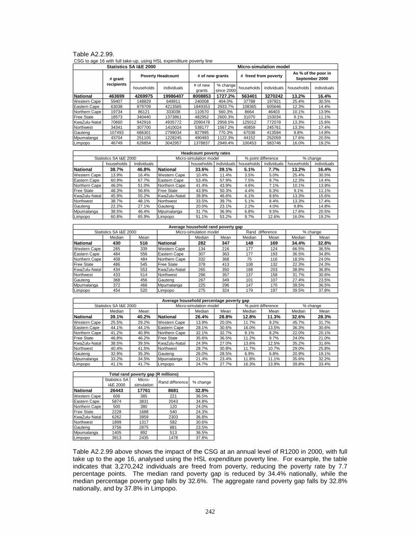
242
Table A2.2.99.
Table A2.2.99 above shows the impact of the CSG at an annual level of R1200 in 2000, with full take up to the age 16, analysed using the HSL expenditure poverty line. For example, the table indicates that 3,270,242 individuals are freed from poverty, reducing the poverty rate by 7.7 percentage points. The median rand poverty gap is reduced by 34.4% nationally, while the median percentage poverty gap falls by 32.6%. The aggregate rand poverty gap falls by 32.8% nationally, and by 37.8% in Limpopo.
CSG to age 16 with full take-up, using HSL expenditure poverty line
households individuals # of new grants
% change since 2000 households individuals households individuals
National 463699 4269975 19986407 8008853 1727.2% 563401 3270242 13.2% 16.4%Western Cape 59407 148829 649911 240008 404.0% 37788 197921 25.4% 30.5%Eastern Cape 63038 879709 4213565 1849353 2933.7% 108365 605646 12.3% 14.4%Northern Cape 19734 86121 333038 110570 560.3% 8664 46403 10.1% 13.9%Free State 18573 340440 1373861 482952 2600.3% 31070 153034 9.1% 11.1%KwaZulu-Natal 70660 942916 4935772 2090478 2958.5% 125012 772078 13.3% 15.6%Northwest 34341 307700 1410024 538177 1567.2% 40859 245761 13.3% 17.4%Gauteng 107493 686301 2799034 827995 770.3% 67038 413594 9.8% 14.8%Mpumalanga 43704 251105 1228245 490483 1122.3% 44152 252059 17.6% 20.5%Limpopo 46749 626854 3042957 1378837 2949.4% 100453 583746 16.0% 19.2%
households individuals households individuals households individuals households individualsNational 38.7% 46.8% National 33.6% 39.1% 5.1% 7.7% 13.2% 16.4%Western Cape 13.9% 16.4% Western Cape 10.4% 11.4% 3.5% 5.0% 25.4% 30.5%Eastern Cape 60.9% 67.7% Eastern Cape 53.4% 57.9% 7.5% 9.7% 12.3% 14.4%Northern Cape 46.0% 51.0% Northern Cape 41.4% 43.9% 4.6% 7.1% 10.1% 13.9%Free State 48.3% 56.6% Free State 43.9% 50.3% 4.4% 6.3% 9.1% 11.1%KwaZulu-Natal 45.9% 55.2% KwaZulu-Natal 39.8% 46.6% 6.1% 8.6% 13.3% 15.6%Northwest 38.7% 48.1% Northwest 33.5% 39.7% 5.1% 8.4% 13.3% 17.4%Gauteng 22.2% 27.1% Gauteng 20.0% 23.1% 2.2% 4.0% 9.8% 14.8%Mpumalanga 38.5% 46.4% Mpumalanga 31.7% 36.9% 6.8% 9.5% 17.6% 20.5%Limpopo 60.8% 65.9% Limpopo 51.1% 53.2% 9.7% 12.6% 16.0% 19.2%
Median Mean Median Mean Median Mean Median MeanNational 430 516 National 282 347 148 169 34.4% 32.8%Western Cape 265 339 Western Cape 134 216 177 124 66.5% 36.5%Eastern Cape 484 556 Eastern Cape 307 363 177 193 36.5% 34.8%Northern Cape 408 484 Northern Cape 332 368 75 116 18.5% 24.0%Free State 486 545 Free State 378 413 108 132 22.3% 24.3%KwaZulu-Natal 434 553 KwaZulu-Natal 265 350 168 203 38.8% 36.8%Northwest 433 514 Northwest 296 357 137 158 31.7% 30.6%Gauteng 368 456 Gauteng 267 349 101 107 27.4% 23.5%Mpumalanga 372 466 Mpumalanga 225 296 147 170 39.5% 36.5%Limpopo 454 520 Limpopo 275 324 179 197 39.5% 37.8%
Median Mean Median Mean Median Mean Median MeanNational 39.1% 40.2% National 26.4% 28.8% 12.8% 11.3% 32.6% 28.3%Western Cape 25.5% 29.2% Western Cape 13.9% 20.0% 11.7% 9.2% 45.7% 31.7%Eastern Cape 44.1% 44.1% Eastern Cape 28.1% 30.6% 16.0% 13.5% 36.3% 30.6%Northern Cape 41.2% 40.9% Northern Cape 32.1% 32.7% 9.1% 8.2% 22.0% 20.1%Free State 46.8% 46.2% Free State 35.6% 36.5% 11.2% 9.7% 24.0% 21.0%KwaZulu-Natal 38.5% 39.5% KwaZulu-Natal 24.9% 27.0% 13.6% 12.5% 35.2% 31.6%Northwest 40.4% 41.5% Northwest 28.7% 30.8% 11.7% 10.7% 29.0% 25.8%Gauteng 32.9% 35.3% Gauteng 26.0% 28.5% 6.9% 6.8% 20.9% 19.1%Mpumalanga 33.2% 34.5% Mpumalanga 21.4% 23.4% 11.8% 11.1% 35.6% 32.2%Limpopo 41.1% 41.7% Limpopo 24.7% 27.7% 16.3% 13.9% 39.8% 33.4%
Statistics SA I&E 2000
Micro-simulation Rand difference % change
National 26443 17761 8681 32.8%Western Cape 606 385 221 36.5%Eastern Cape 5874 3831 2043 34.8%Northern Cape 500 380 120 24.0%Free State 2228 1688 540 24.3%KwaZulu-Natal 6262 3959 2303 36.8%Northwest 1899 1317 582 30.6%Gauteng 3756 2875 881 23.5%Mpumalanga 1405 892 513 36.5%Limpopo 3913 2435 1478 37.8%
Total rand poverty gap (R millions)
Statistics SA I&E 2000 Micro-simulation model
Micro-simulation modelStatistics SA I&E 2000
Poverty Headcount# grant
recipients
% point differenceAverage household percentage poverty gap
Average household rand poverty gap% change
% changeMicro-simulation model
% change
Headcount poverty rates
# of new grants # freed from poverty As % of the poor in September 2000
Statistics SA I&E 2000 % point difference
Statistics SA I&E 2000 Micro-simulation model Rand difference

243
Table A2.2.100.
Table A2.2.100 above shows the impact of the CSG at an annual level of R1200 in 2000, with full take up to the age 18, analysed using the HSL expenditure poverty line. For example, the table indicates that 3,686,839 individuals are freed from poverty, reducing the poverty rate by 8.6 percentage points. The median rand poverty gap is reduced by 38.3% nationally, while the median percentage poverty gap falls by 37.0%. The aggregate rand poverty gap falls by 36.7% nationally, and by 42.0% in Limpopo.
CSG to age 18 with full take-up, using HSL expenditure poverty line
households individuals # of new grants
% change since 2000 households individuals households individuals
National 463699 4269975 19986407 9042075 1950.0% 635465 3686839 14.9% 18.4%Western Cape 59407 148829 649911 269710 454.0% 40775 214882 27.4% 33.1%Eastern Cape 63038 879709 4213565 2091513 3317.9% 122997 691664 14.0% 16.4%Northern Cape 19734 86121 333038 123839 627.5% 9559 49464 11.1% 14.9%Free State 18573 340440 1373861 558742 3008.4% 33372 165727 9.8% 12.1%KwaZulu-Natal 70660 942916 4935772 2348492 3323.7% 145987 908653 15.5% 18.4%Northwest 34341 307700 1410024 602743 1755.2% 47235 275710 15.4% 19.6%Gauteng 107493 686301 2799034 934821 869.7% 75312 457374 11.0% 16.3%Mpumalanga 43704 251105 1228245 561625 1285.1% 49588 285428 19.7% 23.2%Limpopo 46749 626854 3042957 1550590 3316.8% 110640 637937 17.7% 21.0%
households individuals households individuals households individuals households individualsNational 38.7% 46.8% National 33.0% 38.2% 5.8% 8.6% 14.9% 18.4%Western Cape 13.9% 16.4% Western Cape 10.1% 11.0% 3.8% 5.4% 27.4% 33.1%Eastern Cape 60.9% 67.7% Eastern Cape 52.4% 56.6% 8.5% 11.1% 14.0% 16.4%Northern Cape 46.0% 51.0% Northern Cape 40.9% 43.4% 5.1% 7.6% 11.1% 14.9%Free State 48.3% 56.6% Free State 43.6% 49.8% 4.7% 6.8% 9.8% 12.1%KwaZulu-Natal 45.9% 55.2% KwaZulu-Natal 38.8% 45.1% 7.1% 10.2% 15.5% 18.4%Northwest 38.7% 48.1% Northwest 32.7% 38.7% 5.9% 9.4% 15.4% 19.6%Gauteng 22.2% 27.1% Gauteng 19.8% 22.7% 2.4% 4.4% 11.0% 16.3%Mpumalanga 38.5% 46.4% Mpumalanga 30.9% 35.7% 7.6% 10.8% 19.7% 23.2%Limpopo 60.8% 65.9% Limpopo 50.1% 52.1% 10.7% 13.8% 17.7% 21.0%
Median Mean Median Mean Median Mean Median MeanNational 430 516 National 265 327 165 189 38.3% 36.7%Western Cape 265 339 Western Cape 131 200 195 139 73.4% 41.0%Eastern Cape 484 556 Eastern Cape 289 340 195 217 40.3% 39.0%Northern Cape 408 484 Northern Cape 330 354 78 129 19.1% 26.8%Free State 486 545 Free State 368 393 118 153 24.3% 28.0%KwaZulu-Natal 434 553 KwaZulu-Natal 244 327 189 226 43.7% 40.9%Northwest 433 514 Northwest 286 340 147 174 33.9% 33.9%Gauteng 368 456 Gauteng 258 337 109 119 29.8% 26.1%Mpumalanga 372 466 Mpumalanga 213 273 159 193 42.8% 41.3%Limpopo 454 520 Limpopo 252 302 202 218 44.6% 42.0%
Median Mean Median Mean Median Mean Median MeanNational 39.1% 40.2% National 24.6% 27.5% 14.5% 12.7% 37.0% 31.6%Western Cape 25.5% 29.2% Western Cape 13.0% 18.9% 12.5% 10.3% 49.0% 35.3%Eastern Cape 44.1% 44.1% Eastern Cape 26.4% 29.0% 17.7% 15.2% 40.2% 34.4%Northern Cape 41.2% 40.9% Northern Cape 31.9% 31.7% 9.3% 9.1% 22.5% 22.3%Free State 46.8% 46.2% Free State 34.7% 34.9% 12.1% 11.3% 25.8% 24.4%KwaZulu-Natal 38.5% 39.5% KwaZulu-Natal 23.4% 25.7% 15.1% 13.9% 39.2% 35.1%Northwest 40.4% 41.5% Northwest 27.4% 29.7% 13.0% 11.8% 32.2% 28.4%Gauteng 32.9% 35.3% Gauteng 25.1% 27.8% 7.8% 7.5% 23.7% 21.2%Mpumalanga 33.2% 34.5% Mpumalanga 19.5% 22.0% 13.6% 12.5% 41.1% 36.3%Limpopo 41.1% 41.7% Limpopo 22.9% 26.2% 18.1% 15.5% 44.2% 37.1%
Statistics SA I&E 2000
Micro-simulation Rand difference % change
National 26443 16741 9702 36.7%Western Cape 606 357 249 41.0%Eastern Cape 5874 3584 2289 39.0%Northern Cape 500 366 134 26.8%Free State 2228 1604 624 28.0%KwaZulu-Natal 6262 3704 2558 40.9%Northwest 1899 1256 643 33.9%Gauteng 3756 2775 981 26.1%Mpumalanga 1405 824 581 41.3%Limpopo 3913 2271 1642 42.0%
% change
Headcount poverty rates
# of new grants # freed from poverty As % of the poor in September 2000
Statistics SA I&E 2000 % point difference
Statistics SA I&E 2000 Micro-simulation model Rand differenceAverage household rand poverty gap
% change
% changeMicro-simulation model
Total rand poverty gap (R millions)
Statistics SA I&E 2000 Micro-simulation model
Micro-simulation modelStatistics SA I&E 2000
Poverty Headcount# grant
recipients
% point differenceAverage household percentage poverty gap
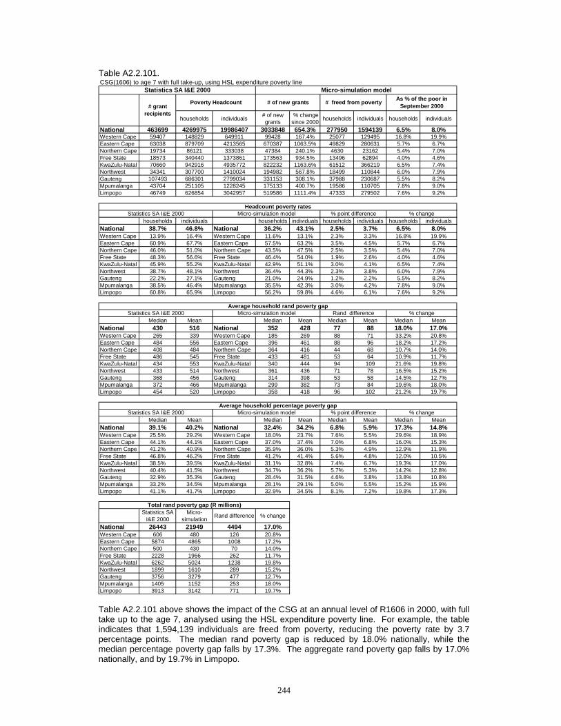
244
Table A2.2.101.
Table A2.2.101 above shows the impact of the CSG at an annual level of R1606 in 2000, with full take up to the age 7, analysed using the HSL expenditure poverty line. For example, the table indicates that 1,594,139 individuals are freed from poverty, reducing the poverty rate by 3.7 percentage points. The median rand poverty gap is reduced by 18.0% nationally, while the median percentage poverty gap falls by 17.3%. The aggregate rand poverty gap falls by 17.0% nationally, and by 19.7% in Limpopo.
CSG(1606) to age 7 with full take-up, using HSL expenditure poverty line
households individuals # of new grants
% change since 2000 households individuals households individuals
National 463699 4269975 19986407 3033848 654.3% 277950 1594139 6.5% 8.0%Western Cape 59407 148829 649911 99428 167.4% 25077 129495 16.8% 19.9%Eastern Cape 63038 879709 4213565 670387 1063.5% 49829 280631 5.7% 6.7%Northern Cape 19734 86121 333038 47384 240.1% 4630 23162 5.4% 7.0%Free State 18573 340440 1373861 173563 934.5% 13496 62894 4.0% 4.6%KwaZulu-Natal 70660 942916 4935772 822232 1163.6% 61512 366219 6.5% 7.4%Northwest 34341 307700 1410024 194982 567.8% 18499 110844 6.0% 7.9%Gauteng 107493 686301 2799034 331153 308.1% 37988 230687 5.5% 8.2%Mpumalanga 43704 251105 1228245 175133 400.7% 19586 110705 7.8% 9.0%Limpopo 46749 626854 3042957 519586 1111.4% 47333 279502 7.6% 9.2%
households individuals households individuals households individuals households individualsNational 38.7% 46.8% National 36.2% 43.1% 2.5% 3.7% 6.5% 8.0%Western Cape 13.9% 16.4% Western Cape 11.6% 13.1% 2.3% 3.3% 16.8% 19.9%Eastern Cape 60.9% 67.7% Eastern Cape 57.5% 63.2% 3.5% 4.5% 5.7% 6.7%Northern Cape 46.0% 51.0% Northern Cape 43.5% 47.5% 2.5% 3.5% 5.4% 7.0%Free State 48.3% 56.6% Free State 46.4% 54.0% 1.9% 2.6% 4.0% 4.6%KwaZulu-Natal 45.9% 55.2% KwaZulu-Natal 42.9% 51.1% 3.0% 4.1% 6.5% 7.4%Northwest 38.7% 48.1% Northwest 36.4% 44.3% 2.3% 3.8% 6.0% 7.9%Gauteng 22.2% 27.1% Gauteng 21.0% 24.9% 1.2% 2.2% 5.5% 8.2%Mpumalanga 38.5% 46.4% Mpumalanga 35.5% 42.3% 3.0% 4.2% 7.8% 9.0%Limpopo 60.8% 65.9% Limpopo 56.2% 59.8% 4.6% 6.1% 7.6% 9.2%
Median Mean Median Mean Median Mean Median MeanNational 430 516 National 352 428 77 88 18.0% 17.0%Western Cape 265 339 Western Cape 185 269 88 71 33.2% 20.8%Eastern Cape 484 556 Eastern Cape 396 461 88 96 18.2% 17.2%Northern Cape 408 484 Northern Cape 364 416 44 68 10.7% 14.0%Free State 486 545 Free State 433 481 53 64 10.9% 11.7%KwaZulu-Natal 434 553 KwaZulu-Natal 340 444 94 109 21.6% 19.8%Northwest 433 514 Northwest 361 436 71 78 16.5% 15.2%Gauteng 368 456 Gauteng 314 398 53 58 14.5% 12.7%Mpumalanga 372 466 Mpumalanga 299 382 73 84 19.6% 18.0%Limpopo 454 520 Limpopo 358 418 96 102 21.2% 19.7%
Median Mean Median Mean Median Mean Median MeanNational 39.1% 40.2% National 32.4% 34.2% 6.8% 5.9% 17.3% 14.8%Western Cape 25.5% 29.2% Western Cape 18.0% 23.7% 7.6% 5.5% 29.6% 18.9%Eastern Cape 44.1% 44.1% Eastern Cape 37.0% 37.4% 7.0% 6.8% 16.0% 15.3%Northern Cape 41.2% 40.9% Northern Cape 35.9% 36.0% 5.3% 4.9% 12.9% 11.9%Free State 46.8% 46.2% Free State 41.2% 41.4% 5.6% 4.8% 12.0% 10.5%KwaZulu-Natal 38.5% 39.5% KwaZulu-Natal 31.1% 32.8% 7.4% 6.7% 19.3% 17.0%Northwest 40.4% 41.5% Northwest 34.7% 36.2% 5.7% 5.3% 14.2% 12.8%Gauteng 32.9% 35.3% Gauteng 28.4% 31.5% 4.6% 3.8% 13.8% 10.8%Mpumalanga 33.2% 34.5% Mpumalanga 28.1% 29.1% 5.0% 5.5% 15.2% 15.9%Limpopo 41.1% 41.7% Limpopo 32.9% 34.5% 8.1% 7.2% 19.8% 17.3%
Statistics SA I&E 2000
Micro-simulation Rand difference % change
National 26443 21949 4494 17.0%Western Cape 606 480 126 20.8%Eastern Cape 5874 4865 1008 17.2%Northern Cape 500 430 70 14.0%Free State 2228 1966 262 11.7%KwaZulu-Natal 6262 5024 1238 19.8%Northwest 1899 1610 289 15.2%Gauteng 3756 3279 477 12.7%Mpumalanga 1405 1152 253 18.0%Limpopo 3913 3142 771 19.7%
Total rand poverty gap (R millions)
Statistics SA I&E 2000 Micro-simulation model
Micro-simulation modelStatistics SA I&E 2000
Poverty Headcount# grant
recipients
% point differenceAverage household percentage poverty gap
Average household rand poverty gap% change
% changeMicro-simulation model
% change
Headcount poverty rates
# of new grants # freed from poverty As % of the poor in September 2000
Statistics SA I&E 2000 % point difference
Statistics SA I&E 2000 Micro-simulation model Rand difference

245
Table A2.2.102.
Table A2.2.102 above shows the impact of the CSG at an annual level of R1606 in 2000, with full take up to the age 9, analysed using the HSL expenditure poverty line. For example, the table indicates that 2,151,375 individuals are freed from poverty, reducing the poverty rate by 5.0 percentage points. The median rand poverty gap is reduced by 23.5% nationally, while the median percentage poverty gap falls by 22.2%. The aggregate rand poverty gap falls by 22.8% nationally, and by 26.1% in Limpopo.
CSG(1606) to age 9 with full take-up, using HSL expenditure poverty line
households individuals # of new grants
% change since 2000 households individuals households individuals
National 463699 4269975 19986407 4108401 886.0% 372366 2151375 8.7% 10.8%Western Cape 59407 148829 649911 129262 217.6% 30390 163644 20.4% 25.2%Eastern Cape 63038 879709 4213565 916100 1453.3% 67417 388537 7.7% 9.2%Northern Cape 19734 86121 333038 60125 304.7% 6455 33313 7.5% 10.0%Free State 18573 340440 1373861 239684 1290.5% 19556 93356 5.7% 6.8%KwaZulu-Natal 70660 942916 4935772 1109800 1570.6% 83429 494175 8.8% 10.0%Northwest 34341 307700 1410024 269057 783.5% 23650 142616 7.7% 10.1%Gauteng 107493 686301 2799034 440699 410.0% 47415 281154 6.9% 10.0%Mpumalanga 43704 251105 1228245 244771 560.1% 27206 155104 10.8% 12.6%Limpopo 46749 626854 3042957 698903 1495.0% 66848 399476 10.7% 13.1%
households individuals households individuals households individuals households individualsNational 38.7% 46.8% National 35.3% 41.7% 3.4% 5.0% 8.7% 10.8%Western Cape 13.9% 16.4% Western Cape 11.1% 12.3% 2.8% 4.1% 20.4% 25.2%Eastern Cape 60.9% 67.7% Eastern Cape 56.3% 61.4% 4.7% 6.2% 7.7% 9.2%Northern Cape 46.0% 51.0% Northern Cape 42.6% 45.9% 3.4% 5.1% 7.5% 10.0%Free State 48.3% 56.6% Free State 45.6% 52.8% 2.8% 3.8% 5.7% 6.8%KwaZulu-Natal 45.9% 55.2% KwaZulu-Natal 41.8% 49.7% 4.1% 5.5% 8.8% 10.0%Northwest 38.7% 48.1% Northwest 35.7% 43.2% 3.0% 4.9% 7.7% 10.1%Gauteng 22.2% 27.1% Gauteng 20.7% 24.4% 1.5% 2.7% 6.9% 10.0%Mpumalanga 38.5% 46.4% Mpumalanga 34.3% 40.6% 4.2% 5.9% 10.8% 12.6%Limpopo 60.8% 65.9% Limpopo 54.3% 57.2% 6.5% 8.6% 10.7% 13.1%
Median Mean Median Mean Median Mean Median MeanNational 430 516 National 329 399 101 117 23.5% 22.8%Western Cape 265 339 Western Cape 158 251 113 89 42.5% 26.1%Eastern Cape 484 556 Eastern Cape 371 427 113 130 23.3% 23.3%Northern Cape 408 484 Northern Cape 348 399 59 85 14.6% 17.5%Free State 486 545 Free State 414 458 72 88 14.7% 16.1%KwaZulu-Natal 434 553 KwaZulu-Natal 311 408 122 145 28.2% 26.3%Northwest 433 514 Northwest 330 408 103 107 23.9% 20.8%Gauteng 368 456 Gauteng 299 380 68 76 18.6% 16.8%Mpumalanga 372 466 Mpumalanga 270 350 102 116 27.3% 25.0%Limpopo 454 520 Limpopo 333 384 121 136 26.7% 26.1%
Median Mean Median Mean Median Mean Median MeanNational 39.1% 40.2% National 30.4% 32.2% 8.7% 7.9% 22.2% 19.7%Western Cape 25.5% 29.2% Western Cape 16.8% 22.4% 8.8% 6.8% 34.4% 23.2%Eastern Cape 44.1% 44.1% Eastern Cape 33.6% 35.0% 10.5% 9.1% 23.8% 20.7%Northern Cape 41.2% 40.9% Northern Cape 34.8% 34.7% 6.3% 6.1% 15.4% 15.0%Free State 46.8% 46.2% Free State 39.3% 39.6% 7.5% 6.6% 16.0% 14.3%KwaZulu-Natal 38.5% 39.5% KwaZulu-Natal 28.7% 30.6% 9.8% 8.9% 25.4% 22.6%Northwest 40.4% 41.5% Northwest 33.4% 34.2% 7.0% 7.3% 17.4% 17.6%Gauteng 32.9% 35.3% Gauteng 27.8% 30.3% 5.1% 5.0% 15.4% 14.2%Mpumalanga 33.2% 34.5% Mpumalanga 25.2% 26.9% 7.9% 7.6% 23.9% 22.0%Limpopo 41.1% 41.7% Limpopo 30.1% 32.1% 11.0% 9.6% 26.8% 23.0%
Statistics SA I&E 2000
Micro-simulation Rand difference % change
National 26443 20427 6016 22.8%Western Cape 606 448 158 26.1%Eastern Cape 5874 4504 1370 23.3%Northern Cape 500 413 87 17.5%Free State 2228 1870 358 16.1%KwaZulu-Natal 6262 4617 1645 26.3%Northwest 1899 1505 394 20.8%Gauteng 3756 3126 630 16.8%Mpumalanga 1405 1054 351 25.0%Limpopo 3913 2890 1023 26.1%
Total rand poverty gap (R millions)
Statistics SA I&E 2000 Micro-simulation model
Micro-simulation modelStatistics SA I&E 2000
Poverty Headcount# grant
recipients
% point differenceAverage household percentage poverty gap
Average household rand poverty gap% change
% changeMicro-simulation model
% change
Headcount poverty rates
# of new grants # freed from poverty As % of the poor in September 2000
Statistics SA I&E 2000 % point difference
Statistics SA I&E 2000 Micro-simulation model Rand difference
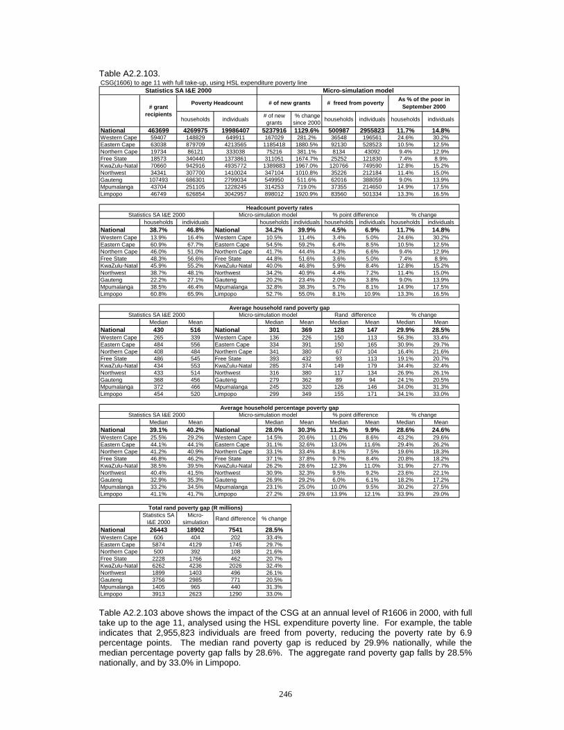
246
Table A2.2.103.
Table A2.2.103 above shows the impact of the CSG at an annual level of R1606 in 2000, with full take up to the age 11, analysed using the HSL expenditure poverty line. For example, the table indicates that 2,955,823 individuals are freed from poverty, reducing the poverty rate by 6.9 percentage points. The median rand poverty gap is reduced by 29.9% nationally, while the median percentage poverty gap falls by 28.6%. The aggregate rand poverty gap falls by 28.5% nationally, and by 33.0% in Limpopo.
CSG(1606) to age 11 with full take-up, using HSL expenditure poverty line
households individuals # of new grants
% change since 2000 households individuals households individuals
National 463699 4269975 19986407 5237916 1129.6% 500987 2955823 11.7% 14.8%Western Cape 59407 148829 649911 167029 281.2% 36548 196561 24.6% 30.2%Eastern Cape 63038 879709 4213565 1185418 1880.5% 92130 528523 10.5% 12.5%Northern Cape 19734 86121 333038 75216 381.1% 8134 43092 9.4% 12.9%Free State 18573 340440 1373861 311051 1674.7% 25252 121830 7.4% 8.9%KwaZulu-Natal 70660 942916 4935772 1389883 1967.0% 120766 749590 12.8% 15.2%Northwest 34341 307700 1410024 347104 1010.8% 35226 212184 11.4% 15.0%Gauteng 107493 686301 2799034 549950 511.6% 62016 388059 9.0% 13.9%Mpumalanga 43704 251105 1228245 314253 719.0% 37355 214650 14.9% 17.5%Limpopo 46749 626854 3042957 898012 1920.9% 83560 501334 13.3% 16.5%
households individuals households individuals households individuals households individualsNational 38.7% 46.8% National 34.2% 39.9% 4.5% 6.9% 11.7% 14.8%Western Cape 13.9% 16.4% Western Cape 10.5% 11.4% 3.4% 5.0% 24.6% 30.2%Eastern Cape 60.9% 67.7% Eastern Cape 54.5% 59.2% 6.4% 8.5% 10.5% 12.5%Northern Cape 46.0% 51.0% Northern Cape 41.7% 44.4% 4.3% 6.6% 9.4% 12.9%Free State 48.3% 56.6% Free State 44.8% 51.6% 3.6% 5.0% 7.4% 8.9%KwaZulu-Natal 45.9% 55.2% KwaZulu-Natal 40.0% 46.8% 5.9% 8.4% 12.8% 15.2%Northwest 38.7% 48.1% Northwest 34.2% 40.9% 4.4% 7.2% 11.4% 15.0%Gauteng 22.2% 27.1% Gauteng 20.2% 23.4% 2.0% 3.8% 9.0% 13.9%Mpumalanga 38.5% 46.4% Mpumalanga 32.8% 38.3% 5.7% 8.1% 14.9% 17.5%Limpopo 60.8% 65.9% Limpopo 52.7% 55.0% 8.1% 10.9% 13.3% 16.5%
Median Mean Median Mean Median Mean Median MeanNational 430 516 National 301 369 128 147 29.9% 28.5%Western Cape 265 339 Western Cape 136 226 150 113 56.3% 33.4%Eastern Cape 484 556 Eastern Cape 334 391 150 165 30.9% 29.7%Northern Cape 408 484 Northern Cape 341 380 67 104 16.4% 21.6%Free State 486 545 Free State 393 432 93 113 19.1% 20.7%KwaZulu-Natal 434 553 KwaZulu-Natal 285 374 149 179 34.4% 32.4%Northwest 433 514 Northwest 316 380 117 134 26.9% 26.1%Gauteng 368 456 Gauteng 279 362 89 94 24.1% 20.5%Mpumalanga 372 466 Mpumalanga 245 320 126 146 34.0% 31.3%Limpopo 454 520 Limpopo 299 349 155 171 34.1% 33.0%
Median Mean Median Mean Median Mean Median MeanNational 39.1% 40.2% National 28.0% 30.3% 11.2% 9.9% 28.6% 24.6%Western Cape 25.5% 29.2% Western Cape 14.5% 20.6% 11.0% 8.6% 43.2% 29.6%Eastern Cape 44.1% 44.1% Eastern Cape 31.1% 32.6% 13.0% 11.6% 29.4% 26.2%Northern Cape 41.2% 40.9% Northern Cape 33.1% 33.4% 8.1% 7.5% 19.6% 18.3%Free State 46.8% 46.2% Free State 37.1% 37.8% 9.7% 8.4% 20.8% 18.2%KwaZulu-Natal 38.5% 39.5% KwaZulu-Natal 26.2% 28.6% 12.3% 11.0% 31.9% 27.7%Northwest 40.4% 41.5% Northwest 30.9% 32.3% 9.5% 9.2% 23.6% 22.1%Gauteng 32.9% 35.3% Gauteng 26.9% 29.2% 6.0% 6.1% 18.2% 17.2%Mpumalanga 33.2% 34.5% Mpumalanga 23.1% 25.0% 10.0% 9.5% 30.2% 27.5%Limpopo 41.1% 41.7% Limpopo 27.2% 29.6% 13.9% 12.1% 33.9% 29.0%
Statistics SA I&E 2000
Micro-simulation Rand difference % change
National 26443 18902 7541 28.5%Western Cape 606 404 202 33.4%Eastern Cape 5874 4129 1745 29.7%Northern Cape 500 392 108 21.6%Free State 2228 1766 462 20.7%KwaZulu-Natal 6262 4236 2026 32.4%Northwest 1899 1403 496 26.1%Gauteng 3756 2985 771 20.5%Mpumalanga 1405 965 440 31.3%Limpopo 3913 2623 1290 33.0%
Total rand poverty gap (R millions)
Statistics SA I&E 2000 Micro-simulation model
Micro-simulation modelStatistics SA I&E 2000
Poverty Headcount# grant
recipients
% point differenceAverage household percentage poverty gap
Average household rand poverty gap% change
% changeMicro-simulation model
% change
Headcount poverty rates
# of new grants # freed from poverty As % of the poor in September 2000
Statistics SA I&E 2000 % point difference
Statistics SA I&E 2000 Micro-simulation model Rand difference

247
Table A2.2.104.
Table A2.2.104 above shows the impact of the CSG at an annual level of R1606 in 2000, with full take up to the age 14, analysed using the HSL expenditure poverty line. For example, the table indicates that 4,038,520 individuals are freed from poverty, reducing the poverty rate by 9.5 percentage points. The median rand poverty gap is reduced by 39.5% nationally, while the median percentage poverty gap falls by 37.6%. The aggregate rand poverty gap falls by 36.7% nationally, and by 42.5% in Limpopo.
CSG(1606) to age 14 with full take-up, using HSL expenditure poverty line
households individuals # of new grants
% change since 2000 households individuals households individuals
National 463699 4269975 19986407 6903080 1488.7% 685356 4038520 16.1% 20.2%Western Cape 59407 148829 649911 208037 350.2% 41289 222380 27.7% 34.2%Eastern Cape 63038 879709 4213565 1587610 2518.5% 136638 783166 15.5% 18.6%Northern Cape 19734 86121 333038 96330 488.1% 9846 52234 11.4% 15.7%Free State 18573 340440 1373861 410471 2210.0% 35978 180749 10.6% 13.2%KwaZulu-Natal 70660 942916 4935772 1804875 2554.3% 157177 988730 16.7% 20.0%Northwest 34341 307700 1410024 463631 1350.1% 46518 275666 15.1% 19.6%Gauteng 107493 686301 2799034 722152 671.8% 89481 548683 13.0% 19.6%Mpumalanga 43704 251105 1228245 419360 959.5% 48994 283741 19.5% 23.1%Limpopo 46749 626854 3042957 1190614 2546.8% 119435 703171 19.1% 23.1%
households individuals households individuals households individuals households individualsNational 38.7% 46.8% National 32.5% 37.3% 6.2% 9.5% 16.0% 20.2%Western Cape 13.9% 16.4% Western Cape 10.1% 10.8% 3.9% 5.6% 27.7% 34.2%Eastern Cape 60.9% 67.7% Eastern Cape 51.5% 55.1% 9.5% 12.6% 15.5% 18.6%Northern Cape 46.0% 51.0% Northern Cape 40.8% 43.0% 5.3% 8.0% 11.4% 15.7%Free State 48.3% 56.6% Free State 43.2% 49.2% 5.1% 7.5% 10.6% 13.2%KwaZulu-Natal 45.9% 55.2% KwaZulu-Natal 38.2% 44.2% 7.6% 11.1% 16.7% 20.0%Northwest 38.7% 48.1% Northwest 32.8% 38.7% 5.8% 9.4% 15.1% 19.6%Gauteng 22.2% 27.1% Gauteng 19.3% 21.8% 2.9% 5.3% 13.0% 19.6%Mpumalanga 38.5% 46.4% Mpumalanga 31.0% 35.7% 7.5% 10.7% 19.5% 23.1%Limpopo 60.8% 65.9% Limpopo 49.2% 50.7% 11.6% 15.2% 19.1% 23.1%
Median Mean Median Mean Median Mean Median MeanNational 430 516 National 260 326 170 190 39.5% 36.7%Western Cape 265 339 Western Cape 128 204 196 135 73.9% 39.9%Eastern Cape 484 556 Eastern Cape 287 340 196 216 40.6% 38.9%Northern Cape 408 484 Northern Cape 322 352 85 132 20.9% 27.3%Free State 486 545 Free State 360 398 126 147 26.0% 27.0%KwaZulu-Natal 434 553 KwaZulu-Natal 240 326 194 228 44.7% 41.1%Northwest 433 514 Northwest 281 338 152 177 35.1% 34.4%Gauteng 368 456 Gauteng 255 336 112 120 30.5% 26.4%Mpumalanga 372 466 Mpumalanga 209 277 163 189 43.9% 40.5%Limpopo 454 520 Limpopo 240 299 215 221 47.2% 42.5%
Median Mean Median Mean Median Mean Median MeanNational 39.1% 40.2% National 24.4% 27.5% 14.7% 12.7% 37.6% 31.6%Western Cape 25.5% 29.2% Western Cape 12.8% 19.0% 12.8% 10.2% 50.0% 34.9%Eastern Cape 44.1% 44.1% Eastern Cape 26.2% 29.1% 17.9% 15.0% 40.6% 34.1%Northern Cape 41.2% 40.9% Northern Cape 29.2% 31.5% 11.9% 9.3% 29.0% 22.9%Free State 46.8% 46.2% Free State 34.1% 35.4% 12.7% 10.8% 27.1% 23.5%KwaZulu-Natal 38.5% 39.5% KwaZulu-Natal 22.7% 25.6% 15.8% 13.9% 41.0% 35.2%Northwest 40.4% 41.5% Northwest 27.3% 29.5% 13.1% 12.0% 32.4% 28.9%Gauteng 32.9% 35.3% Gauteng 25.1% 27.7% 7.8% 7.6% 23.7% 21.6%Mpumalanga 33.2% 34.5% Mpumalanga 19.2% 22.3% 13.9% 12.3% 42.0% 35.5%Limpopo 41.1% 41.7% Limpopo 22.4% 26.0% 18.7% 15.6% 45.5% 37.5%
Statistics SA I&E 2000
Micro-simulation Rand difference % change
National 26443 16731 9712 36.7%Western Cape 606 364 242 39.9%Eastern Cape 5874 3591 2283 38.9%Northern Cape 500 364 136 27.3%Free State 2228 1626 602 27.0%KwaZulu-Natal 6262 3687 2575 41.1%Northwest 1899 1246 652 34.4%Gauteng 3756 2766 990 26.4%Mpumalanga 1405 836 569 40.5%Limpopo 3913 2250 1663 42.5%
% change
Headcount poverty rates
# of new grants # freed from poverty As % of the poor in September 2000
Statistics SA I&E 2000 % point difference
Statistics SA I&E 2000 Micro-simulation model Rand differenceAverage household rand poverty gap
% change
% changeMicro-simulation model
Total rand poverty gap (R millions)
Statistics SA I&E 2000 Micro-simulation model
Micro-simulation modelStatistics SA I&E 2000
Poverty Headcount# grant
recipients
% point differenceAverage household percentage poverty gap
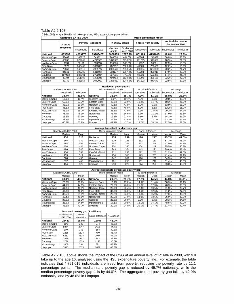
248
Table A2.2.105.
Table A2.2.105 above shows the impact of the CSG at an annual level of R1606 in 2000, with full take up to the age 16, analysed using the HSL expenditure poverty line. For example, the table indicates that 4,751,015 individuals are freed from poverty, reducing the poverty rate by 11.1 percentage points. The median rand poverty gap is reduced by 45.7% nationally, while the median percentage poverty gap falls by 44.0%. The aggregate rand poverty gap falls by 42.0% nationally, and by 48.0% in Limpopo.
CSG(1606) to age 16 with full take-up, using HSL expenditure poverty line
households individuals # of new grants
% change since 2000 households individuals households individuals
National 463699 4269975 19986407 8008853 1727.2% 801199 4751015 18.8% 23.8%Western Cape 59407 148829 649911 240008 404.0% 45804 249027 30.8% 38.3%Eastern Cape 63038 879709 4213565 1849353 2933.7% 161295 917669 18.3% 21.8%Northern Cape 19734 86121 333038 110570 560.3% 11092 59801 12.9% 18.0%Free State 18573 340440 1373861 482952 2600.3% 41389 208421 12.2% 15.2%KwaZulu-Natal 70660 942916 4935772 2090478 2958.5% 190084 1219002 20.2% 24.7%Northwest 34341 307700 1410024 538177 1567.2% 55204 328915 17.9% 23.3%Gauteng 107493 686301 2799034 827995 770.3% 96739 592379 14.1% 21.2%Mpumalanga 43704 251105 1228245 490483 1122.3% 58399 335158 23.3% 27.3%Limpopo 46749 626854 3042957 1378837 2949.4% 141193 840643 22.5% 27.6%
households individuals households individuals households individuals households individualsNational 38.7% 46.8% National 31.5% 35.7% 7.3% 11.1% 18.8% 23.8%Western Cape 13.9% 16.4% Western Cape 9.6% 10.1% 4.3% 6.3% 30.8% 38.3%Eastern Cape 60.9% 67.7% Eastern Cape 49.8% 52.9% 11.2% 14.7% 18.3% 21.8%Northern Cape 46.0% 51.0% Northern Cape 40.1% 41.9% 5.9% 9.2% 12.9% 18.0%Free State 48.3% 56.6% Free State 42.5% 48.0% 5.9% 8.6% 12.2% 15.2%KwaZulu-Natal 45.9% 55.2% KwaZulu-Natal 36.6% 41.6% 9.3% 13.6% 20.2% 24.7%Northwest 38.7% 48.1% Northwest 31.7% 36.9% 6.9% 11.2% 17.9% 23.3%Gauteng 22.2% 27.1% Gauteng 19.1% 21.4% 3.1% 5.7% 14.1% 21.2%Mpumalanga 38.5% 46.4% Mpumalanga 29.6% 33.8% 9.0% 12.7% 23.3% 27.3%Limpopo 60.8% 65.9% Limpopo 47.1% 47.7% 13.7% 18.2% 22.5% 27.6%
Median Mean Median Mean Median Mean Median MeanNational 430 516 National 233 299 196 217 45.7% 42.0%Western Cape 265 339 Western Cape 110 186 232 153 87.3% 45.2%Eastern Cape 484 556 Eastern Cape 252 308 232 249 47.9% 44.7%Northern Cape 408 484 Northern Cape 304 335 104 149 25.5% 30.8%Free State 486 545 Free State 343 374 143 171 29.4% 31.4%KwaZulu-Natal 434 553 KwaZulu-Natal 211 293 222 260 51.2% 47.0%Northwest 433 514 Northwest 254 313 179 201 41.4% 39.1%Gauteng 368 456 Gauteng 242 319 126 137 34.3% 30.0%Mpumalanga 372 466 Mpumalanga 181 250 191 216 51.4% 46.3%Limpopo 454 520 Limpopo 210 270 244 250 53.8% 48.0%
Median Mean Median Mean Median Mean Median MeanNational 39.1% 40.2% National 21.9% 25.7% 17.2% 14.5% 44.0% 36.1%Western Cape 25.5% 29.2% Western Cape 10.7% 17.8% 14.9% 11.4% 58.3% 39.1%Eastern Cape 44.1% 44.1% Eastern Cape 22.8% 26.8% 21.3% 17.3% 48.3% 39.3%Northern Cape 41.2% 40.9% Northern Cape 28.3% 30.4% 12.9% 10.5% 31.3% 25.7%Free State 46.8% 46.2% Free State 32.2% 33.6% 14.6% 12.6% 31.2% 27.3%KwaZulu-Natal 38.5% 39.5% KwaZulu-Natal 20.2% 23.6% 18.3% 15.9% 47.6% 40.3%Northwest 40.4% 41.5% Northwest 25.5% 27.9% 14.9% 13.6% 36.9% 32.8%Gauteng 32.9% 35.3% Gauteng 23.6% 26.6% 9.3% 8.7% 28.1% 24.5%Mpumalanga 33.2% 34.5% Mpumalanga 17.1% 20.5% 16.1% 14.1% 48.6% 40.7%Limpopo 41.1% 41.7% Limpopo 20.0% 24.0% 21.1% 17.7% 51.4% 42.4%
Statistics SA I&E 2000
Micro-simulation Rand difference % change
National 26443 15345 11098 42.0%Western Cape 606 332 274 45.2%Eastern Cape 5874 3247 2626 44.7%Northern Cape 500 346 154 30.8%Free State 2228 1528 700 31.4%KwaZulu-Natal 6262 3318 2944 47.0%Northwest 1899 1157 742 39.1%Gauteng 3756 2629 1127 30.0%Mpumalanga 1405 754 651 46.3%Limpopo 3913 2033 1879 48.0%
% change
Headcount poverty rates
# of new grants # freed from poverty As % of the poor in September 2000
Statistics SA I&E 2000 % point difference
Statistics SA I&E 2000 Micro-simulation model Rand differenceAverage household rand poverty gap
% change
% changeMicro-simulation model
Total rand poverty gap (R millions)
Statistics SA I&E 2000 Micro-simulation model
Micro-simulation modelStatistics SA I&E 2000
Poverty Headcount# grant
recipients
% point differenceAverage household percentage poverty gap

249
Table A2.2.106.
Table A2.2.106 above shows the impact of the CSG at an annual level of R1606 in 2000, with full take up to the age 18, analysed using the HSL expenditure poverty line. For example, the table indicates that 5,435,113 individuals are freed from poverty, reducing the poverty rate by 12.7 percentage points. The median rand poverty gap is reduced by 50.8% nationally, while the median percentage poverty gap falls by 49.8%. The aggregate rand poverty gap falls by 46.6% nationally, and by 53.0% in Limpopo.
CSG(1606) to age 18 with full take-up, using HSL expenditure poverty line
households individuals # of new grants
% change since 2000 households individuals households individuals
National 463699 4269975 19986407 9042075 1950.0% 915300 5435113 21.4% 27.2%Western Cape 59407 148829 649911 269710 454.0% 50424 275660 33.9% 42.4%Eastern Cape 63038 879709 4213565 2091513 3317.9% 189162 1098019 21.5% 26.1%Northern Cape 19734 86121 333038 123839 627.5% 12629 65084 14.7% 19.5%Free State 18573 340440 1373861 558742 3008.4% 48925 249314 14.4% 18.1%KwaZulu-Natal 70660 942916 4935772 2348492 3323.7% 217591 1389595 23.1% 28.2%Northwest 34341 307700 1410024 602743 1755.2% 60593 352434 19.7% 25.0%Gauteng 107493 686301 2799034 934821 869.7% 104622 637058 15.2% 22.8%Mpumalanga 43704 251105 1228245 561625 1285.1% 65085 377084 25.9% 30.7%Limpopo 46749 626854 3042957 1550590 3316.8% 166269 990865 26.5% 32.6%
households individuals households individuals households individuals households individualsNational 38.7% 46.8% National 30.4% 34.1% 8.3% 12.7% 21.4% 27.2%Western Cape 13.9% 16.4% Western Cape 9.2% 9.4% 4.7% 6.9% 33.9% 42.4%Eastern Cape 60.9% 67.7% Eastern Cape 47.8% 50.0% 13.1% 17.6% 21.5% 26.1%Northern Cape 46.0% 51.0% Northern Cape 39.3% 41.0% 6.7% 10.0% 14.7% 19.5%Free State 48.3% 56.6% Free State 41.4% 46.4% 6.9% 10.3% 14.4% 18.1%KwaZulu-Natal 45.9% 55.2% KwaZulu-Natal 35.3% 39.7% 10.6% 15.5% 23.1% 28.2%Northwest 38.7% 48.1% Northwest 31.1% 36.1% 7.6% 12.0% 19.7% 25.0%Gauteng 22.2% 27.1% Gauteng 18.8% 21.0% 3.4% 6.2% 15.2% 22.8%Mpumalanga 38.5% 46.4% Mpumalanga 28.5% 32.2% 10.0% 14.3% 25.9% 30.7%Limpopo 60.8% 65.9% Limpopo 44.7% 44.4% 16.1% 21.5% 26.5% 32.6%
Median Mean Median Mean Median Mean Median MeanNational 430 516 National 211 275 218 241 50.8% 46.6%Western Cape 265 339 Western Cape 93 168 258 171 97.1% 50.5%Eastern Cape 484 556 Eastern Cape 226 280 258 277 53.3% 49.7%Northern Cape 408 484 Northern Cape 296 318 112 166 27.4% 34.2%Free State 486 545 Free State 320 348 166 198 34.1% 36.2%KwaZulu-Natal 434 553 KwaZulu-Natal 191 266 243 287 56.0% 51.9%Northwest 433 514 Northwest 236 292 197 222 45.5% 43.2%Gauteng 368 456 Gauteng 229 304 138 152 37.6% 33.4%Mpumalanga 372 466 Mpumalanga 159 223 213 244 57.2% 52.2%Limpopo 454 520 Limpopo 182 245 272 276 60.0% 53.0%
Median Mean Median Mean Median Mean Median MeanNational 39.1% 40.2% National 19.7% 24.0% 19.5% 16.1% 49.8% 40.1%Western Cape 25.5% 29.2% Western Cape 9.5% 16.5% 16.1% 12.7% 62.9% 43.4%Eastern Cape 44.1% 44.1% Eastern Cape 20.0% 24.8% 24.1% 19.3% 54.6% 43.8%Northern Cape 41.2% 40.9% Northern Cape 28.0% 29.2% 13.2% 11.7% 32.0% 28.6%Free State 46.8% 46.2% Free State 30.8% 31.6% 16.0% 14.6% 34.2% 31.6%KwaZulu-Natal 38.5% 39.5% KwaZulu-Natal 18.4% 22.0% 20.1% 17.6% 52.3% 44.4%Northwest 40.4% 41.5% Northwest 23.6% 26.5% 16.8% 15.0% 41.6% 36.1%Gauteng 32.9% 35.3% Gauteng 22.0% 25.7% 10.9% 9.6% 33.2% 27.2%Mpumalanga 33.2% 34.5% Mpumalanga 14.5% 18.7% 18.6% 15.8% 56.1% 45.8%Limpopo 41.1% 41.7% Limpopo 16.9% 22.1% 24.1% 19.5% 58.7% 46.9%
Statistics SA I&E 2000
Micro-simulation Rand difference % change
National 26443 14108 12335 46.6%Western Cape 606 300 306 50.5%Eastern Cape 5874 2952 2922 49.7%Northern Cape 500 329 171 34.2%Free State 2228 1421 807 36.2%KwaZulu-Natal 6262 3013 3248 51.9%Northwest 1899 1079 820 43.2%Gauteng 3756 2502 1254 33.4%Mpumalanga 1405 671 734 52.2%Limpopo 3913 1840 2073 53.0%
% change
Headcount poverty rates
# of new grants # freed from poverty As % of the poor in September 2000
Statistics SA I&E 2000 % point difference
Statistics SA I&E 2000 Micro-simulation model Rand differenceAverage household rand poverty gap
% change
% changeMicro-simulation model
Total rand poverty gap (R millions)
Statistics SA I&E 2000 Micro-simulation model
Micro-simulation modelStatistics SA I&E 2000
Poverty Headcount# grant
recipients
% point differenceAverage household percentage poverty gap

250
Table A2.2.107.
Table A2.2.107 above shows the impact of all grants with full take up, with the CSG at an annual level of R1200 in 2000, analysed using the HSL expenditure poverty line. For example, the table indicates that 4,683,960 individuals are freed from poverty, reducing the poverty rate by 11.0 percentage points. The median rand poverty gap is reduced by 44.8% nationally, while the median percentage poverty gap falls by 42.2%. The aggregate rand poverty gap falls by 39.4% nationally, and by 41.9% in Limpopo.
All grants with full take-up, using HSL expenditure poverty line
households individuals # of new grants
% change since 2000 households individuals households individuals
National 2656508 4269975 19986407 8076935 304.0% 863921 4683960 20.2% 23.4%Western Cape 241897 148829 649911 291669 120.6% 48600 241164 32.7% 37.1%Eastern Cape 499290 879709 4213565 1813152 363.1% 183219 934980 20.8% 22.2%Northern Cape 69402 86121 333038 125540 180.9% 16357 78521 19.0% 23.6%Free State 131645 340440 1373861 486486 369.5% 48215 238819 14.2% 17.4%KwaZulu-Natal 522017 942916 4935772 2044876 391.7% 190002 1095353 20.2% 22.2%Northwest 208084 307700 1410024 564671 271.4% 72068 390787 23.4% 27.7%Gauteng 471943 686301 2799034 961901 203.8% 119340 668597 17.4% 23.9%Mpumalanga 161387 251105 1228245 484707 300.3% 58346 326554 23.2% 26.6%Limpopo 350843 626854 3042957 1303933 371.7% 127774 709185 20.4% 23.3%
households individuals households individuals households individuals households individualsNational 38.7% 46.8% National 30.9% 35.8% 7.8% 11.0% 20.2% 23.4%Western Cape 13.9% 16.4% Western Cape 9.4% 10.3% 4.5% 6.1% 32.7% 37.1%Eastern Cape 60.9% 67.7% Eastern Cape 48.2% 52.7% 12.7% 15.0% 20.8% 22.2%Northern Cape 46.0% 51.0% Northern Cape 37.3% 39.0% 8.7% 12.0% 19.0% 23.6%Free State 48.3% 56.6% Free State 41.5% 46.8% 6.8% 9.8% 14.2% 17.4%KwaZulu-Natal 45.9% 55.2% KwaZulu-Natal 36.6% 43.0% 9.2% 12.3% 20.2% 22.2%Northwest 38.7% 48.1% Northwest 29.6% 34.8% 9.1% 13.3% 23.4% 27.7%Gauteng 22.2% 27.1% Gauteng 18.3% 20.7% 3.9% 6.5% 17.4% 23.9%Mpumalanga 38.5% 46.4% Mpumalanga 29.6% 34.1% 8.9% 12.3% 23.2% 26.6%Limpopo 60.8% 65.9% Limpopo 48.4% 50.5% 12.4% 15.4% 20.4% 23.3%
Median Mean Median Mean Median Mean Median MeanNational 430 516 National 237 313 192 203 44.8% 39.4%Western Cape 265 339 Western Cape 126 200 216 139 81.5% 40.9%Eastern Cape 484 556 Eastern Cape 267 323 216 233 44.8% 41.9%Northern Cape 408 484 Northern Cape 259 317 149 167 36.6% 34.4%Free State 486 545 Free State 349 380 137 165 28.1% 30.3%KwaZulu-Natal 434 553 KwaZulu-Natal 223 317 211 236 48.6% 42.7%Northwest 433 514 Northwest 228 302 204 213 47.2% 41.3%Gauteng 368 456 Gauteng 228 312 139 144 37.8% 31.6%Mpumalanga 372 466 Mpumalanga 191 272 181 195 48.6% 41.7%Limpopo 454 520 Limpopo 242 302 212 218 46.8% 41.9%
Median Mean Median Mean Median Mean Median MeanNational 39.1% 40.2% National 22.6% 26.1% 16.5% 14.1% 42.2% 35.1%Western Cape 25.5% 29.2% Western Cape 12.6% 18.2% 12.9% 11.0% 50.5% 37.6%Eastern Cape 44.1% 44.1% Eastern Cape 24.2% 27.2% 19.8% 16.9% 45.0% 38.3%Northern Cape 41.2% 40.9% Northern Cape 26.8% 28.6% 14.4% 12.3% 34.9% 30.0%Free State 46.8% 46.2% Free State 32.8% 33.9% 14.0% 12.3% 29.9% 26.6%KwaZulu-Natal 38.5% 39.5% KwaZulu-Natal 21.2% 24.5% 17.3% 15.0% 45.0% 37.9%Northwest 40.4% 41.5% Northwest 22.2% 26.4% 18.3% 15.1% 45.2% 36.5%Gauteng 32.9% 35.3% Gauteng 22.3% 25.9% 10.6% 9.4% 32.1% 26.6%Mpumalanga 33.2% 34.5% Mpumalanga 17.6% 21.7% 15.6% 12.8% 46.9% 37.1%Limpopo 41.1% 41.7% Limpopo 22.1% 25.8% 19.0% 15.8% 46.2% 38.0%
Statistics SA I&E 2000
Micro-simulation Rand difference % change
National 26443 16016 10427 39.4%Western Cape 606 358 248 40.9%Eastern Cape 5874 3412 2462 41.9%Northern Cape 500 328 172 34.4%Free State 2228 1554 674 30.3%KwaZulu-Natal 6262 3591 2671 42.7%Northwest 1899 1114 785 41.3%Gauteng 3756 2568 1188 31.6%Mpumalanga 1405 819 586 41.7%Limpopo 3913 2272 1640 41.9%
% change
Headcount poverty rates
# of new grants # freed from poverty As % of the poor in September 2000
Statistics SA I&E 2000 % point difference
Statistics SA I&E 2000 Micro-simulation model Rand differenceAverage household rand poverty gap
% change
% changeMicro-simulation model
Total rand poverty gap (R millions)
Statistics SA I&E 2000 Micro-simulation model
Micro-simulation modelStatistics SA I&E 2000
Poverty Headcount# grant
recipients
% point differenceAverage household percentage poverty gap
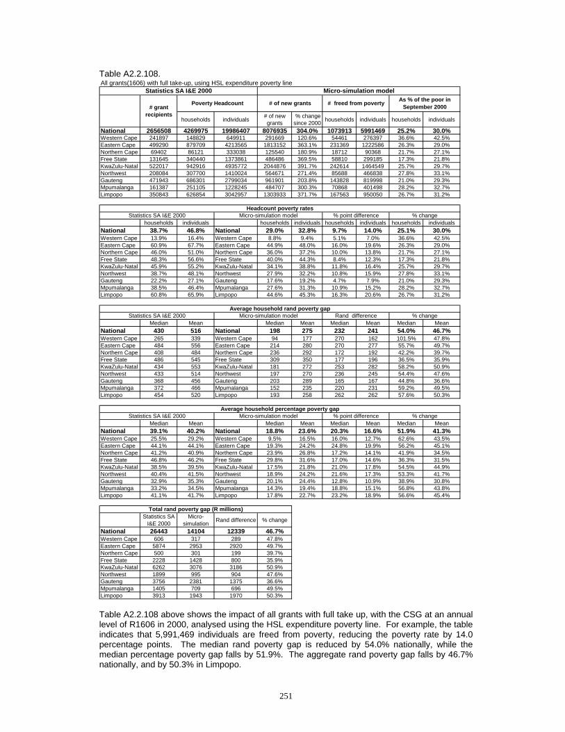
251
Table A2.2.108.
Table A2.2.108 above shows the impact of all grants with full take up, with the CSG at an annual level of R1606 in 2000, analysed using the HSL expenditure poverty line. For example, the table indicates that 5,991,469 individuals are freed from poverty, reducing the poverty rate by 14.0 percentage points. The median rand poverty gap is reduced by 54.0% nationally, while the median percentage poverty gap falls by 51.9%. The aggregate rand poverty gap falls by 46.7% nationally, and by 50.3% in Limpopo.
All grants(1606) with full take-up, using HSL expenditure poverty line
households individuals # of new grants
% change since 2000 households individuals households individuals
National 2656508 4269975 19986407 8076935 304.0% 1073913 5991469 25.2% 30.0%Western Cape 241897 148829 649911 291669 120.6% 54461 276397 36.6% 42.5%Eastern Cape 499290 879709 4213565 1813152 363.1% 231369 1222586 26.3% 29.0%Northern Cape 69402 86121 333038 125540 180.9% 18712 90368 21.7% 27.1%Free State 131645 340440 1373861 486486 369.5% 58810 299185 17.3% 21.8%KwaZulu-Natal 522017 942916 4935772 2044876 391.7% 242614 1464549 25.7% 29.7%Northwest 208084 307700 1410024 564671 271.4% 85688 466838 27.8% 33.1%Gauteng 471943 686301 2799034 961901 203.8% 143828 819998 21.0% 29.3%Mpumalanga 161387 251105 1228245 484707 300.3% 70868 401498 28.2% 32.7%Limpopo 350843 626854 3042957 1303933 371.7% 167563 950050 26.7% 31.2%
households individuals households individuals households individuals households individualsNational 38.7% 46.8% National 29.0% 32.8% 9.7% 14.0% 25.1% 30.0%Western Cape 13.9% 16.4% Western Cape 8.8% 9.4% 5.1% 7.0% 36.6% 42.5%Eastern Cape 60.9% 67.7% Eastern Cape 44.9% 48.0% 16.0% 19.6% 26.3% 29.0%Northern Cape 46.0% 51.0% Northern Cape 36.0% 37.2% 10.0% 13.8% 21.7% 27.1%Free State 48.3% 56.6% Free State 40.0% 44.3% 8.4% 12.3% 17.3% 21.8%KwaZulu-Natal 45.9% 55.2% KwaZulu-Natal 34.1% 38.8% 11.8% 16.4% 25.7% 29.7%Northwest 38.7% 48.1% Northwest 27.9% 32.2% 10.8% 15.9% 27.8% 33.1%Gauteng 22.2% 27.1% Gauteng 17.6% 19.2% 4.7% 7.9% 21.0% 29.3%Mpumalanga 38.5% 46.4% Mpumalanga 27.6% 31.3% 10.9% 15.2% 28.2% 32.7%Limpopo 60.8% 65.9% Limpopo 44.6% 45.3% 16.3% 20.6% 26.7% 31.2%
Median Mean Median Mean Median Mean Median MeanNational 430 516 National 198 275 232 241 54.0% 46.7%Western Cape 265 339 Western Cape 94 177 270 162 101.5% 47.8%Eastern Cape 484 556 Eastern Cape 214 280 270 277 55.7% 49.7%Northern Cape 408 484 Northern Cape 236 292 172 192 42.2% 39.7%Free State 486 545 Free State 309 350 177 196 36.5% 35.9%KwaZulu-Natal 434 553 KwaZulu-Natal 181 272 253 282 58.2% 50.9%Northwest 433 514 Northwest 197 270 236 245 54.4% 47.6%Gauteng 368 456 Gauteng 203 289 165 167 44.8% 36.6%Mpumalanga 372 466 Mpumalanga 152 235 220 231 59.2% 49.5%Limpopo 454 520 Limpopo 193 258 262 262 57.6% 50.3%
Median Mean Median Mean Median Mean Median MeanNational 39.1% 40.2% National 18.8% 23.6% 20.3% 16.6% 51.9% 41.3%Western Cape 25.5% 29.2% Western Cape 9.5% 16.5% 16.0% 12.7% 62.6% 43.5%Eastern Cape 44.1% 44.1% Eastern Cape 19.3% 24.2% 24.8% 19.9% 56.2% 45.1%Northern Cape 41.2% 40.9% Northern Cape 23.9% 26.8% 17.2% 14.1% 41.9% 34.5%Free State 46.8% 46.2% Free State 29.8% 31.6% 17.0% 14.6% 36.3% 31.5%KwaZulu-Natal 38.5% 39.5% KwaZulu-Natal 17.5% 21.8% 21.0% 17.8% 54.5% 44.9%Northwest 40.4% 41.5% Northwest 18.9% 24.2% 21.6% 17.3% 53.3% 41.7%Gauteng 32.9% 35.3% Gauteng 20.1% 24.4% 12.8% 10.9% 38.9% 30.8%Mpumalanga 33.2% 34.5% Mpumalanga 14.3% 19.4% 18.8% 15.1% 56.8% 43.8%Limpopo 41.1% 41.7% Limpopo 17.8% 22.7% 23.2% 18.9% 56.6% 45.4%
Statistics SA I&E 2000
Micro-simulation Rand difference % change
National 26443 14104 12339 46.7%Western Cape 606 317 289 47.8%Eastern Cape 5874 2953 2920 49.7%Northern Cape 500 301 199 39.7%Free State 2228 1428 800 35.9%KwaZulu-Natal 6262 3076 3186 50.9%Northwest 1899 995 904 47.6%Gauteng 3756 2381 1375 36.6%Mpumalanga 1405 709 696 49.5%Limpopo 3913 1943 1970 50.3%
Total rand poverty gap (R millions)
Statistics SA I&E 2000 Micro-simulation model
Micro-simulation modelStatistics SA I&E 2000
Poverty Headcount# grant
recipients
% point differenceAverage household percentage poverty gap
Average household rand poverty gap% change
% changeMicro-simulation model
% change
Headcount poverty rates
# of new grants # freed from poverty As % of the poor in September 2000
Statistics SA I&E 2000 % point difference
Statistics SA I&E 2000 Micro-simulation model Rand difference
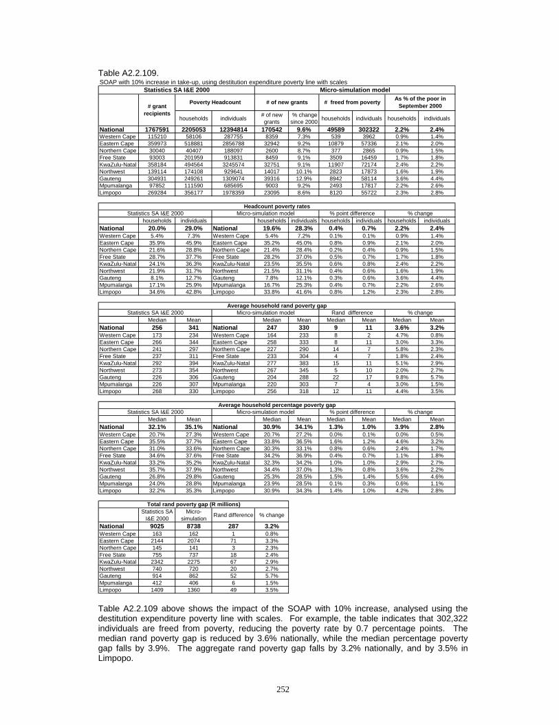
252
Table A2.2.109.
Table A2.2.109 above shows the impact of the SOAP with 10% increase, analysed using the destitution expenditure poverty line with scales. For example, the table indicates that 302,322 individuals are freed from poverty, reducing the poverty rate by 0.7 percentage points. The median rand poverty gap is reduced by 3.6% nationally, while the median percentage poverty gap falls by 3.9%. The aggregate rand poverty gap falls by 3.2% nationally, and by 3.5% in Limpopo.
SOAP with 10% increase in take-up, using destitution expenditure poverty line with scales
households individuals # of new grants
% change since 2000 households individuals households individuals
National 1767591 2205053 12394814 170542 9.6% 49589 302322 2.2% 2.4%Western Cape 115210 58106 287755 8359 7.3% 539 3962 0.9% 1.4%Eastern Cape 359973 518881 2856788 32942 9.2% 10879 57336 2.1% 2.0%Northern Cape 30040 40407 188097 2600 8.7% 377 2865 0.9% 1.5%Free State 93003 201959 913831 8459 9.1% 3509 16459 1.7% 1.8%KwaZulu-Natal 358184 494564 3245574 32751 9.1% 11907 72174 2.4% 2.2%Northwest 139114 174108 929641 14017 10.1% 2823 17873 1.6% 1.9%Gauteng 304931 249261 1309074 39316 12.9% 8942 58114 3.6% 4.4%Mpumalanga 97852 111590 685695 9003 9.2% 2493 17817 2.2% 2.6%Limpopo 269284 356177 1978359 23095 8.6% 8120 55722 2.3% 2.8%
households individuals households individuals households individuals households individualsNational 20.0% 29.0% National 19.6% 28.3% 0.4% 0.7% 2.2% 2.4%Western Cape 5.4% 7.3% Western Cape 5.4% 7.2% 0.1% 0.1% 0.9% 1.4%Eastern Cape 35.9% 45.9% Eastern Cape 35.2% 45.0% 0.8% 0.9% 2.1% 2.0%Northern Cape 21.6% 28.8% Northern Cape 21.4% 28.4% 0.2% 0.4% 0.9% 1.5%Free State 28.7% 37.7% Free State 28.2% 37.0% 0.5% 0.7% 1.7% 1.8%KwaZulu-Natal 24.1% 36.3% KwaZulu-Natal 23.5% 35.5% 0.6% 0.8% 2.4% 2.2%Northwest 21.9% 31.7% Northwest 21.5% 31.1% 0.4% 0.6% 1.6% 1.9%Gauteng 8.1% 12.7% Gauteng 7.8% 12.1% 0.3% 0.6% 3.6% 4.4%Mpumalanga 17.1% 25.9% Mpumalanga 16.7% 25.3% 0.4% 0.7% 2.2% 2.6%Limpopo 34.6% 42.8% Limpopo 33.8% 41.6% 0.8% 1.2% 2.3% 2.8%
Median Mean Median Mean Median Mean Median MeanNational 256 341 National 247 330 9 11 3.6% 3.2%Western Cape 173 234 Western Cape 164 233 8 2 4.7% 0.8%Eastern Cape 266 344 Eastern Cape 258 333 8 11 3.0% 3.3%Northern Cape 241 297 Northern Cape 227 290 14 7 5.8% 2.3%Free State 237 311 Free State 233 304 4 7 1.8% 2.4%KwaZulu-Natal 292 394 KwaZulu-Natal 277 383 15 11 5.1% 2.9%Northwest 273 354 Northwest 267 345 5 10 2.0% 2.7%Gauteng 226 306 Gauteng 204 288 22 17 9.8% 5.7%Mpumalanga 226 307 Mpumalanga 220 303 7 4 3.0% 1.5%Limpopo 268 330 Limpopo 256 318 12 11 4.4% 3.5%
Median Mean Median Mean Median Mean Median MeanNational 32.1% 35.1% National 30.9% 34.1% 1.3% 1.0% 3.9% 2.8%Western Cape 20.7% 27.3% Western Cape 20.7% 27.2% 0.0% 0.1% 0.0% 0.5%Eastern Cape 35.5% 37.7% Eastern Cape 33.8% 36.5% 1.6% 1.2% 4.6% 3.2%Northern Cape 31.0% 33.6% Northern Cape 30.3% 33.1% 0.8% 0.6% 2.4% 1.7%Free State 34.6% 37.6% Free State 34.2% 36.9% 0.4% 0.7% 1.1% 1.8%KwaZulu-Natal 33.2% 35.2% KwaZulu-Natal 32.3% 34.2% 1.0% 1.0% 2.9% 2.7%Northwest 35.7% 37.9% Northwest 34.4% 37.0% 1.3% 0.8% 3.6% 2.2%Gauteng 26.8% 29.8% Gauteng 25.3% 28.5% 1.5% 1.4% 5.5% 4.6%Mpumalanga 24.0% 28.8% Mpumalanga 23.9% 28.5% 0.1% 0.3% 0.6% 1.1%Limpopo 32.2% 35.3% Limpopo 30.9% 34.3% 1.4% 1.0% 4.2% 2.8%
Statistics SA I&E 2000
Micro-simulation Rand difference % change
National 9025 8738 287 3.2%Western Cape 163 162 1 0.8%Eastern Cape 2144 2074 71 3.3%Northern Cape 145 141 3 2.3%Free State 755 737 18 2.4%KwaZulu-Natal 2342 2275 67 2.9%Northwest 740 720 20 2.7%Gauteng 914 862 52 5.7%Mpumalanga 412 406 6 1.5%Limpopo 1409 1360 49 3.5%
% change
Headcount poverty rates
# of new grants # freed from poverty As % of the poor in September 2000
Statistics SA I&E 2000 % point difference
Statistics SA I&E 2000 Micro-simulation model Rand differenceAverage household rand poverty gap
% change
% changeMicro-simulation model
Total rand poverty gap (R millions)
Statistics SA I&E 2000 Micro-simulation model
Micro-simulation modelStatistics SA I&E 2000
Poverty Headcount# grant
recipients
% point differenceAverage household percentage poverty gap

253
Table A2.2.110.
Table A2.2.110 above shows the impact of the SOAP with full take up, analysed using the destitution expenditure poverty line with scales. For example, the table indicates that 563,506 individuals are freed from poverty, reducing the poverty rate by 1.3 percentage points. The median rand poverty gap is reduced by 6.7% nationally, while the median percentage poverty gap falls by 7.1%. The aggregate rand poverty gap falls by 6.2% nationally, and by 5.0% in Limpopo.
SOAP with full take-up, using destitution expenditure poverty line with scales
households individuals # of new grants
% change since 2000 households individuals households individuals
National 1767591 2205053 12394814 417730 23.6% 99190 563506 4.5% 4.5%Western Cape 115210 58106 287755 28838 25.0% 1974 5397 3.4% 1.9%Eastern Cape 359973 518881 2856788 80962 22.5% 24228 124066 4.7% 4.3%Northern Cape 30040 40407 188097 7490 24.9% 1140 6160 2.8% 3.3%Free State 93003 201959 913831 22720 24.4% 7251 32602 3.6% 3.6%KwaZulu-Natal 358184 494564 3245574 87472 24.4% 27005 162391 5.5% 5.0%Northwest 139114 174108 929641 28155 20.2% 6395 33417 3.7% 3.6%Gauteng 304931 249261 1309074 109732 36.0% 13339 90559 5.4% 6.9%Mpumalanga 97852 111590 685695 12845 13.1% 3334 22442 3.0% 3.3%Limpopo 269284 356177 1978359 39516 14.7% 14524 86472 4.1% 4.4%
households individuals households individuals households individuals households individualsNational 20.0% 29.0% National 19.1% 27.7% 0.9% 1.3% 4.5% 4.5%Western Cape 5.4% 7.3% Western Cape 5.3% 7.1% 0.2% 0.1% 3.4% 1.9%Eastern Cape 35.9% 45.9% Eastern Cape 34.3% 43.9% 1.7% 2.0% 4.7% 4.3%Northern Cape 21.6% 28.8% Northern Cape 21.0% 27.9% 0.6% 0.9% 2.8% 3.3%Free State 28.7% 37.7% Free State 27.6% 36.3% 1.0% 1.3% 3.6% 3.6%KwaZulu-Natal 24.1% 36.3% KwaZulu-Natal 22.8% 34.5% 1.3% 1.8% 5.5% 5.0%Northwest 21.9% 31.7% Northwest 21.1% 30.6% 0.8% 1.1% 3.7% 3.6%Gauteng 8.1% 12.7% Gauteng 7.6% 11.8% 0.4% 0.9% 5.4% 6.9%Mpumalanga 17.1% 25.9% Mpumalanga 16.6% 25.1% 0.5% 0.8% 3.0% 3.3%Limpopo 34.6% 42.8% Limpopo 33.2% 41.0% 1.4% 1.9% 4.1% 4.4%
Median Mean Median Mean Median Mean Median MeanNational 256 341 National 239 320 17 21 6.7% 6.2%Western Cape 173 234 Western Cape 164 230 14 5 8.3% 2.0%Eastern Cape 266 344 Eastern Cape 252 321 14 23 5.4% 6.7%Northern Cape 241 297 Northern Cape 217 281 24 16 10.0% 5.4%Free State 237 311 Free State 223 292 14 20 5.8% 6.4%KwaZulu-Natal 292 394 KwaZulu-Natal 257 368 34 26 11.8% 6.7%Northwest 273 354 Northwest 259 335 14 20 5.2% 5.5%Gauteng 226 306 Gauteng 192 280 35 26 15.3% 8.5%Mpumalanga 226 307 Mpumalanga 220 302 7 5 3.0% 1.7%Limpopo 268 330 Limpopo 246 313 22 17 8.2% 5.0%
Median Mean Median Mean Median Mean Median MeanNational 32.1% 35.1% National 29.9% 33.1% 2.3% 2.0% 7.1% 5.6%Western Cape 20.7% 27.3% Western Cape 20.3% 26.0% 0.4% 1.3% 1.9% 4.7%Eastern Cape 35.5% 37.7% Eastern Cape 32.5% 35.2% 3.0% 2.4% 8.4% 6.5%Northern Cape 31.0% 33.6% Northern Cape 29.7% 32.0% 1.3% 1.7% 4.2% 4.9%Free State 34.6% 37.6% Free State 32.7% 35.6% 1.9% 2.0% 5.4% 5.4%KwaZulu-Natal 33.2% 35.2% KwaZulu-Natal 30.7% 32.9% 2.5% 2.3% 7.5% 6.5%Northwest 35.7% 37.9% Northwest 33.5% 36.0% 2.2% 1.8% 6.2% 4.9%Gauteng 26.8% 29.8% Gauteng 25.1% 27.9% 1.8% 2.0% 6.6% 6.5%Mpumalanga 24.0% 28.8% Mpumalanga 23.9% 28.4% 0.1% 0.4% 0.6% 1.3%Limpopo 32.2% 35.3% Limpopo 30.2% 33.7% 2.0% 1.6% 6.3% 4.5%
Statistics SA I&E 2000
Micro-simulation Rand difference % change
National 9025 8469 556 6.2%Western Cape 163 160 3 2.0%Eastern Cape 2144 2000 145 6.7%Northern Cape 145 137 8 5.4%Free State 755 707 48 6.4%KwaZulu-Natal 2342 2186 156 6.7%Northwest 740 699 41 5.5%Gauteng 914 836 78 8.5%Mpumalanga 412 405 7 1.7%Limpopo 1409 1338 71 5.0%
% change
Headcount poverty rates
# of new grants # freed from poverty As % of the poor in September 2000
Statistics SA I&E 2000 % point difference
Statistics SA I&E 2000 Micro-simulation model Rand differenceAverage household rand poverty gap
% change
% changeMicro-simulation model
Total rand poverty gap (R millions)
Statistics SA I&E 2000 Micro-simulation model
Micro-simulation modelStatistics SA I&E 2000
Poverty Headcount# grant
recipients
% point differenceAverage household percentage poverty gap
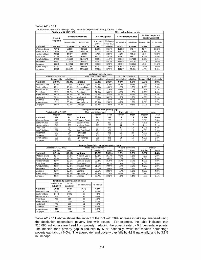
254
Table A2.2.111.
Table A2.2.111 above shows the impact of the DG with 50% increase in take up, analysed using the destitution expenditure poverty line with scales. For example, the table indicates that 916,096 individuals are freed from poverty, reducing the poverty rate by 0.8 percentage points. The median rand poverty gap is reduced by 5.2% nationally, while the median percentage poverty gap falls by 6.0%. The aggregate rand poverty gap falls by 4.8% nationally, and by 3.3% in Limpopo.
DG with 50% increase in take-up, using destitution expenditure poverty line with scales
households individuals # of new grants
% change since 2000 households individuals households individuals
National 438542 2205053 12394814 219203 50.0% 184047 916096 8.3% 7.4%Western Cape 70442 58106 287755 18805 26.7% 17282 74547 29.7% 25.9%Eastern Cape 78664 518881 2856788 42725 54.3% 35529 174419 6.8% 6.1%Northern Cape 20076 40407 188097 5753 28.7% 4528 20142 11.2% 10.7%Free State 20069 201959 913831 15315 76.3% 13007 68523 6.4% 7.5%KwaZulu-Natal 97038 494564 3245574 40651 41.9% 33012 167444 6.7% 5.2%Northwest 34942 174108 929641 22057 63.1% 18655 95176 10.7% 10.2%Gauteng 61745 249261 1309074 38562 62.5% 31799 153450 12.8% 11.7%Mpumalanga 20091 111590 685695 14782 73.6% 12948 70945 11.6% 10.3%Limpopo 35475 356177 1978359 20553 57.9% 17287 91450 4.9% 4.6%
households individuals households individuals households individuals households individualsNational 20.0% 29.0% National 19.4% 28.2% 0.6% 0.8% 3.0% 2.9%Western Cape 5.4% 7.3% Western Cape 5.2% 6.9% 0.2% 0.3% 3.9% 4.5%Eastern Cape 35.9% 45.9% Eastern Cape 34.8% 44.6% 1.1% 1.3% 3.2% 2.9%Northern Cape 21.6% 28.8% Northern Cape 20.8% 27.6% 0.8% 1.2% 3.7% 4.1%Free State 28.7% 37.7% Free State 27.8% 36.2% 0.9% 1.5% 3.2% 4.0%KwaZulu-Natal 24.1% 36.3% KwaZulu-Natal 23.4% 35.4% 0.7% 0.9% 2.8% 2.4%Northwest 21.9% 31.7% Northwest 20.9% 30.1% 1.0% 1.6% 4.6% 5.1%Gauteng 8.1% 12.7% Gauteng 7.9% 12.4% 0.2% 0.3% 2.7% 2.2%Mpumalanga 17.1% 25.9% Mpumalanga 16.5% 25.0% 0.6% 1.0% 3.6% 3.7%Limpopo 34.6% 42.8% Limpopo 33.9% 42.0% 0.7% 0.8% 2.0% 2.0%
Median Mean Median Mean Median Mean Median MeanNational 256 341 National 243 325 13 16 5.2% 4.6%Western Cape 173 234 Western Cape 153 220 12 15 7.0% 6.3%Eastern Cape 266 344 Eastern Cape 254 329 12 15 4.5% 4.5%Northern Cape 241 297 Northern Cape 207 270 34 27 14.2% 9.1%Free State 237 311 Free State 217 298 20 14 8.2% 4.4%KwaZulu-Natal 292 394 KwaZulu-Natal 273 379 18 15 6.3% 3.9%Northwest 273 354 Northwest 254 331 18 23 6.7% 6.5%Gauteng 226 306 Gauteng 213 286 13 19 5.6% 6.3%Mpumalanga 226 307 Mpumalanga 212 291 14 16 6.3% 5.3%Limpopo 268 330 Limpopo 259 319 9 11 3.4% 3.3%
Median Mean Median Mean Median Mean Median MeanNational 32.1% 35.1% National 30.2% 33.5% 1.9% 1.5% 6.0% 4.4%Western Cape 20.7% 27.3% Western Cape 19.8% 25.7% 0.9% 1.6% 4.5% 5.9%Eastern Cape 35.5% 37.7% Eastern Cape 33.1% 35.9% 2.3% 1.8% 6.6% 4.8%Northern Cape 31.0% 33.6% Northern Cape 28.3% 31.0% 2.7% 2.7% 8.7% 7.9%Free State 34.6% 37.6% Free State 33.2% 36.1% 1.4% 1.5% 4.0% 4.0%KwaZulu-Natal 33.2% 35.2% KwaZulu-Natal 31.5% 33.9% 1.7% 1.3% 5.2% 3.8%Northwest 35.7% 37.9% Northwest 33.1% 35.6% 2.6% 2.2% 7.4% 5.9%Gauteng 26.8% 29.8% Gauteng 25.1% 28.3% 1.7% 1.5% 6.5% 4.9%Mpumalanga 24.0% 28.8% Mpumalanga 23.5% 27.6% 0.5% 1.3% 2.2% 4.4%Limpopo 32.2% 35.3% Limpopo 30.7% 34.2% 1.5% 1.1% 4.8% 3.1%
Statistics SA I&E 2000
Micro-simulation Rand difference % change
National 9025 8594 431 4.8%Western Cape 163 153 10 6.3%Eastern Cape 2144 2045 99 4.6%Northern Cape 145 131 14 9.4%Free State 755 719 36 4.8%KwaZulu-Natal 2342 2247 95 4.0%Northwest 740 689 51 6.9%Gauteng 914 856 58 6.3%Mpumalanga 412 390 23 5.5%Limpopo 1409 1363 46 3.3%
% change
Headcount poverty rates
# of new grants # freed from poverty As % of the poor in September 2000
Statistics SA I&E 2000 % point difference
Statistics SA I&E 2000 Micro-simulation model Rand differenceAverage household rand poverty gap
% change
% changeMicro-simulation model
Total rand poverty gap (R millions)
Statistics SA I&E 2000 Micro-simulation model
Micro-simulation modelStatistics SA I&E 2000
Poverty Headcount# grant
recipients
% point differenceAverage household percentage poverty gap
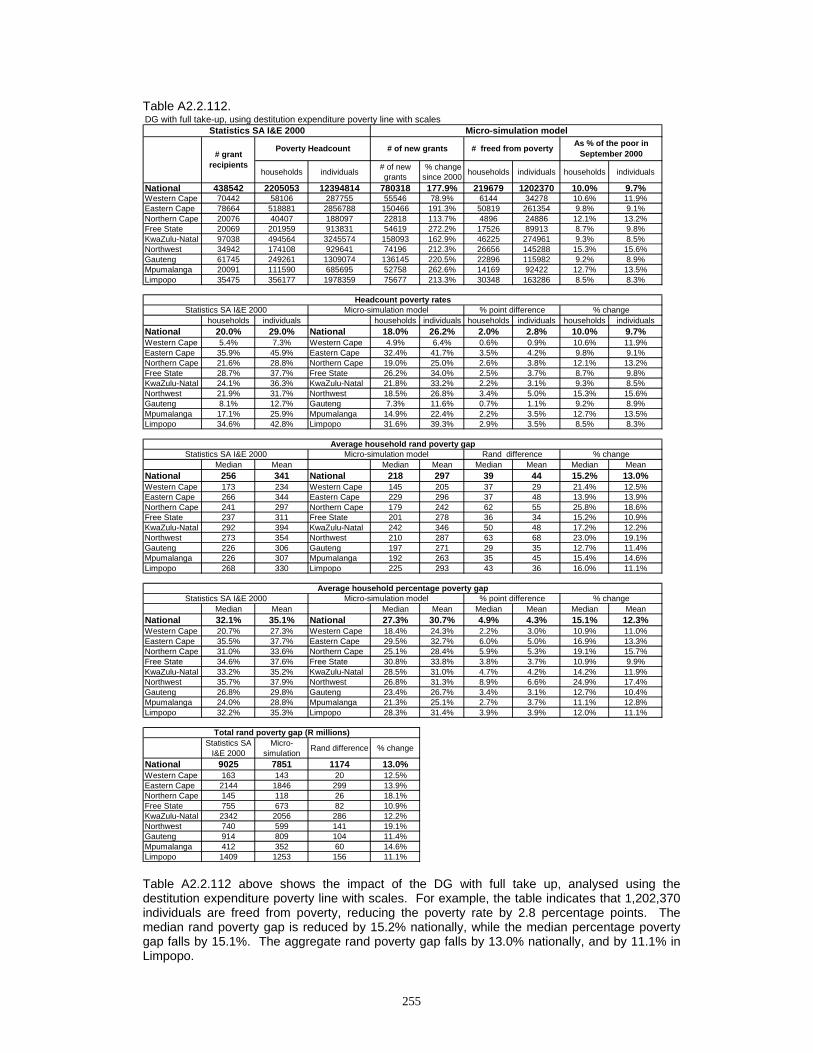
255
Table A2.2.112.
Table A2.2.112 above shows the impact of the DG with full take up, analysed using the destitution expenditure poverty line with scales. For example, the table indicates that 1,202,370 individuals are freed from poverty, reducing the poverty rate by 2.8 percentage points. The median rand poverty gap is reduced by 15.2% nationally, while the median percentage poverty gap falls by 15.1%. The aggregate rand poverty gap falls by 13.0% nationally, and by 11.1% in Limpopo.
DG with full take-up, using destitution expenditure poverty line with scales
households individuals # of new grants
% change since 2000 households individuals households individuals
National 438542 2205053 12394814 780318 177.9% 219679 1202370 10.0% 9.7%Western Cape 70442 58106 287755 55546 78.9% 6144 34278 10.6% 11.9%Eastern Cape 78664 518881 2856788 150466 191.3% 50819 261354 9.8% 9.1%Northern Cape 20076 40407 188097 22818 113.7% 4896 24886 12.1% 13.2%Free State 20069 201959 913831 54619 272.2% 17526 89913 8.7% 9.8%KwaZulu-Natal 97038 494564 3245574 158093 162.9% 46225 274961 9.3% 8.5%Northwest 34942 174108 929641 74196 212.3% 26656 145288 15.3% 15.6%Gauteng 61745 249261 1309074 136145 220.5% 22896 115982 9.2% 8.9%Mpumalanga 20091 111590 685695 52758 262.6% 14169 92422 12.7% 13.5%Limpopo 35475 356177 1978359 75677 213.3% 30348 163286 8.5% 8.3%
households individuals households individuals households individuals households individualsNational 20.0% 29.0% National 18.0% 26.2% 2.0% 2.8% 10.0% 9.7%Western Cape 5.4% 7.3% Western Cape 4.9% 6.4% 0.6% 0.9% 10.6% 11.9%Eastern Cape 35.9% 45.9% Eastern Cape 32.4% 41.7% 3.5% 4.2% 9.8% 9.1%Northern Cape 21.6% 28.8% Northern Cape 19.0% 25.0% 2.6% 3.8% 12.1% 13.2%Free State 28.7% 37.7% Free State 26.2% 34.0% 2.5% 3.7% 8.7% 9.8%KwaZulu-Natal 24.1% 36.3% KwaZulu-Natal 21.8% 33.2% 2.2% 3.1% 9.3% 8.5%Northwest 21.9% 31.7% Northwest 18.5% 26.8% 3.4% 5.0% 15.3% 15.6%Gauteng 8.1% 12.7% Gauteng 7.3% 11.6% 0.7% 1.1% 9.2% 8.9%Mpumalanga 17.1% 25.9% Mpumalanga 14.9% 22.4% 2.2% 3.5% 12.7% 13.5%Limpopo 34.6% 42.8% Limpopo 31.6% 39.3% 2.9% 3.5% 8.5% 8.3%
Median Mean Median Mean Median Mean Median MeanNational 256 341 National 218 297 39 44 15.2% 13.0%Western Cape 173 234 Western Cape 145 205 37 29 21.4% 12.5%Eastern Cape 266 344 Eastern Cape 229 296 37 48 13.9% 13.9%Northern Cape 241 297 Northern Cape 179 242 62 55 25.8% 18.6%Free State 237 311 Free State 201 278 36 34 15.2% 10.9%KwaZulu-Natal 292 394 KwaZulu-Natal 242 346 50 48 17.2% 12.2%Northwest 273 354 Northwest 210 287 63 68 23.0% 19.1%Gauteng 226 306 Gauteng 197 271 29 35 12.7% 11.4%Mpumalanga 226 307 Mpumalanga 192 263 35 45 15.4% 14.6%Limpopo 268 330 Limpopo 225 293 43 36 16.0% 11.1%
Median Mean Median Mean Median Mean Median MeanNational 32.1% 35.1% National 27.3% 30.7% 4.9% 4.3% 15.1% 12.3%Western Cape 20.7% 27.3% Western Cape 18.4% 24.3% 2.2% 3.0% 10.9% 11.0%Eastern Cape 35.5% 37.7% Eastern Cape 29.5% 32.7% 6.0% 5.0% 16.9% 13.3%Northern Cape 31.0% 33.6% Northern Cape 25.1% 28.4% 5.9% 5.3% 19.1% 15.7%Free State 34.6% 37.6% Free State 30.8% 33.8% 3.8% 3.7% 10.9% 9.9%KwaZulu-Natal 33.2% 35.2% KwaZulu-Natal 28.5% 31.0% 4.7% 4.2% 14.2% 11.9%Northwest 35.7% 37.9% Northwest 26.8% 31.3% 8.9% 6.6% 24.9% 17.4%Gauteng 26.8% 29.8% Gauteng 23.4% 26.7% 3.4% 3.1% 12.7% 10.4%Mpumalanga 24.0% 28.8% Mpumalanga 21.3% 25.1% 2.7% 3.7% 11.1% 12.8%Limpopo 32.2% 35.3% Limpopo 28.3% 31.4% 3.9% 3.9% 12.0% 11.1%
Statistics SA I&E 2000
Micro-simulation Rand difference % change
National 9025 7851 1174 13.0%Western Cape 163 143 20 12.5%Eastern Cape 2144 1846 299 13.9%Northern Cape 145 118 26 18.1%Free State 755 673 82 10.9%KwaZulu-Natal 2342 2056 286 12.2%Northwest 740 599 141 19.1%Gauteng 914 809 104 11.4%Mpumalanga 412 352 60 14.6%Limpopo 1409 1253 156 11.1%
% change
Headcount poverty rates
# of new grants # freed from poverty As % of the poor in September 2000
Statistics SA I&E 2000 % point difference
Statistics SA I&E 2000 Micro-simulation model Rand differenceAverage household rand poverty gap
% change
% changeMicro-simulation model
Total rand poverty gap (R millions)
Statistics SA I&E 2000 Micro-simulation model
Micro-simulation modelStatistics SA I&E 2000
Poverty Headcount# grant
recipients
% point differenceAverage household percentage poverty gap

256
Table A2.2.113.
Table A2.2.113 above shows the impact of the CSG at an annual level of R1200 in 2000, with full take up to the age 7, analysed using the destitution expenditure poverty line with scales. For example, the table indicates that 1,448,854 individuals are freed from poverty, reducing the poverty rate by 3.4 percentage points. The median rand poverty gap is reduced by 28.2% nationally, while the median percentage poverty gap falls by 25.6%. The aggregate rand poverty gap falls by 23.0% nationally, and by 25.7% in Limpopo.
CSG to age 7 with full take-up, using destitution expenditure poverty line with scales
households individuals # of new grants
% change since 2000 households individuals households individuals
National 463699 2200788 13316315 2320241 500.4% 244227 1448854 11.1% 10.9%Western Cape 59407 55111 302993 50923 85.7% 10291 56333 18.7% 18.6%Eastern Cape 63038 531349 3076074 549628 871.9% 54053 312821 10.2% 10.2%Northern Cape 19734 35660 190811 31219 158.2% 3361 18679 9.4% 9.8%Free State 18573 192035 937503 135622 730.2% 20051 104287 10.4% 11.1%KwaZulu-Natal 70660 505623 3511949 672028 951.1% 53916 333092 10.7% 9.5%Northwest 34341 165412 960219 152488 444.0% 12801 82311 7.7% 8.6%Gauteng 107493 227113 1365952 176377 164.1% 29404 164390 12.9% 12.0%Mpumalanga 43704 117363 767171 127010 290.6% 17279 109310 14.7% 14.2%Limpopo 46749 371122 2203643 424946 909.0% 43071 267631 11.6% 12.1%
households individuals households individuals households individuals households individualsNational 20.0% 31.2% National 17.7% 27.8% 2.2% 3.4% 11.1% 10.9%Western Cape 5.2% 7.6% Western Cape 4.2% 6.2% 1.0% 1.4% 18.7% 18.6%Eastern Cape 36.8% 49.4% Eastern Cape 33.1% 44.4% 3.7% 5.0% 10.2% 10.2%Northern Cape 19.1% 29.2% Northern Cape 17.3% 26.4% 1.8% 2.9% 9.4% 9.8%Free State 27.3% 38.6% Free State 24.4% 34.4% 2.8% 4.3% 10.4% 11.1%KwaZulu-Natal 24.6% 39.3% KwaZulu-Natal 22.0% 35.6% 2.6% 3.7% 10.7% 9.5%Northwest 20.8% 32.8% Northwest 19.2% 29.9% 1.6% 2.8% 7.7% 8.6%Gauteng 7.3% 13.2% Gauteng 6.4% 11.6% 1.0% 1.6% 12.9% 12.0%Mpumalanga 18.0% 29.0% Mpumalanga 15.3% 24.9% 2.6% 4.1% 14.7% 14.2%Limpopo 36.0% 47.7% Limpopo 31.8% 41.9% 4.2% 5.8% 11.6% 12.1%
Median Mean Median Mean Median Mean Median MeanNational 313 419 National 225 323 88 96 28.2% 23.0%Western Cape 209 276 Western Cape 114 196 92 80 43.9% 28.9%Eastern Cape 343 425 Eastern Cape 251 329 92 95 26.7% 22.4%Northern Cape 268 361 Northern Cape 203 282 64 79 24.1% 21.8%Free State 262 343 Free State 203 280 58 62 22.3% 18.2%KwaZulu-Natal 377 505 KwaZulu-Natal 269 382 108 123 28.7% 24.4%Northwest 343 427 Northwest 262 341 80 85 23.5% 20.0%Gauteng 239 345 Gauteng 157 277 83 67 34.5% 19.5%Mpumalanga 276 388 Mpumalanga 192 295 84 93 30.5% 24.1%Limpopo 321 410 Limpopo 215 305 106 105 33.0% 25.7%
Median Mean Median Mean Median Mean Median MeanNational 34.9% 36.8% National 26.0% 28.9% 8.9% 7.9% 25.6% 21.4%Western Cape 22.2% 28.3% Western Cape 13.9% 20.7% 8.3% 7.6% 37.5% 26.8%Eastern Cape 38.5% 39.7% Eastern Cape 29.3% 31.4% 9.2% 8.2% 23.9% 20.7%Northern Cape 36.1% 36.1% Northern Cape 26.7% 28.8% 9.5% 7.2% 26.2% 20.1%Free State 35.3% 37.9% Free State 28.4% 31.4% 6.9% 6.5% 19.5% 17.1%KwaZulu-Natal 36.9% 37.6% KwaZulu-Natal 27.8% 28.9% 9.1% 8.7% 24.8% 23.1%Northwest 38.3% 39.9% Northwest 29.2% 32.9% 9.2% 7.0% 23.9% 17.5%Gauteng 26.3% 29.0% Gauteng 19.4% 23.3% 6.8% 5.7% 26.0% 19.7%Mpumalanga 26.1% 31.0% Mpumalanga 19.2% 23.8% 6.9% 7.1% 26.5% 23.1%Limpopo 35.7% 37.4% Limpopo 24.8% 28.5% 10.9% 8.9% 30.5% 23.8%
Statistics SA I&E 2000
Micro-simulation Rand difference % change
National 11060 8521 2540 23.0%Western Cape 185 132 53 28.9%Eastern Cape 2707 2100 607 22.4%Northern Cape 155 121 34 21.8%Free State 790 646 144 18.2%KwaZulu-Natal 3064 2316 748 24.4%Northwest 847 677 170 20.0%Gauteng 940 756 184 19.5%Mpumalanga 546 415 131 24.1%Limpopo 1826 1358 468 25.7%
% change
Headcount poverty rates
# of new grants # freed from poverty As % of the poor in September 2000
Statistics SA I&E 2000 % point difference
Statistics SA I&E 2000 Micro-simulation model Rand differenceAverage household rand poverty gap
% change
% changeMicro-simulation model
Total rand poverty gap (R millions)
Statistics SA I&E 2000 Micro-simulation model
Micro-simulation modelStatistics SA I&E 2000
Poverty Headcount# grant
recipients
% point differenceAverage household percentage poverty gap

257
Table A2.2.114.
Table A2.2.114 above shows the impact of the CSG at an annual level of R1200 in 2000, with full take up to the age 9, analysed using the destitution expenditure poverty line with scales. For example, the table indicates that 2,081,908 individuals are freed from poverty, reducing the poverty rate by 4.9 percentage points. The median rand poverty gap is reduced by 36.8% nationally, while the median percentage poverty gap falls by 34.8%. The aggregate rand poverty gap falls by 30.3% nationally, and by 33.5% in Limpopo.
CSG to age 9 with full take-up, using destitution expenditure poverty line with scales
households individuals # of new grants
% change since 2000 households individuals households individuals
National 463699 2200788 13316315 3132856 675.6% 349160 2081908 15.9% 15.6%Western Cape 59407 55111 302993 63471 106.8% 11867 67998 21.5% 22.4%Eastern Cape 63038 531349 3076074 746214 1183.8% 77702 447749 14.6% 14.6%Northern Cape 19734 35660 190811 39625 200.8% 4641 25720 13.0% 13.5%Free State 18573 192035 937503 184231 991.9% 26216 130002 13.7% 13.9%KwaZulu-Natal 70660 505623 3511949 901740 1276.2% 77774 500822 15.4% 14.3%Northwest 34341 165412 960219 208895 608.3% 21243 129750 12.8% 13.5%Gauteng 107493 227113 1365952 247971 230.7% 46772 275211 20.6% 20.1%Mpumalanga 43704 117363 767171 175101 400.7% 23870 147718 20.3% 19.3%Limpopo 46749 371122 2203643 565608 1209.9% 59075 356938 15.9% 16.2%
households individuals households individuals households individuals households individualsNational 20.0% 31.2% National 16.8% 26.3% 3.2% 4.9% 15.9% 15.6%Western Cape 5.2% 7.6% Western Cape 4.0% 5.9% 1.1% 1.7% 21.5% 22.4%Eastern Cape 36.8% 49.4% Eastern Cape 31.4% 42.2% 5.4% 7.2% 14.6% 14.6%Northern Cape 19.1% 29.2% Northern Cape 16.6% 25.3% 2.5% 3.9% 13.0% 13.5%Free State 27.3% 38.6% Free State 23.5% 33.3% 3.7% 5.4% 13.7% 13.9%KwaZulu-Natal 24.6% 39.3% KwaZulu-Natal 20.8% 33.7% 3.8% 5.6% 15.4% 14.3%Northwest 20.8% 32.8% Northwest 18.1% 28.3% 2.7% 4.4% 12.8% 13.5%Gauteng 7.3% 13.2% Gauteng 5.8% 10.6% 1.5% 2.7% 20.6% 20.1%Mpumalanga 18.0% 29.0% Mpumalanga 14.3% 23.4% 3.7% 5.6% 20.3% 19.3%Limpopo 36.0% 47.7% Limpopo 30.3% 40.0% 5.7% 7.7% 15.9% 16.2%
Median Mean Median Mean Median Mean Median MeanNational 313 419 National 198 292 115 127 36.8% 30.3%Western Cape 209 276 Western Cape 96 178 120 98 57.6% 35.4%Eastern Cape 343 425 Eastern Cape 223 298 120 127 35.1% 29.9%Northern Cape 268 361 Northern Cape 173 265 95 96 35.5% 26.7%Free State 262 343 Free State 178 259 84 84 32.0% 24.5%KwaZulu-Natal 377 505 KwaZulu-Natal 224 343 154 162 40.8% 32.0%Northwest 343 427 Northwest 234 312 109 115 31.8% 26.8%Gauteng 239 345 Gauteng 139 254 100 91 41.8% 26.4%Mpumalanga 276 388 Mpumalanga 167 261 109 127 39.7% 32.7%Limpopo 321 410 Limpopo 188 273 133 137 41.5% 33.5%
Median Mean Median Mean Median Mean Median MeanNational 34.9% 36.8% National 22.7% 26.3% 12.1% 10.4% 34.8% 28.4%Western Cape 22.2% 28.3% Western Cape 13.2% 19.1% 9.0% 9.2% 40.7% 32.5%Eastern Cape 38.5% 39.7% Eastern Cape 25.2% 28.7% 13.3% 10.9% 34.5% 27.6%Northern Cape 36.1% 36.1% Northern Cape 24.1% 27.0% 12.0% 9.0% 33.3% 25.0%Free State 35.3% 37.9% Free State 24.5% 29.1% 10.8% 8.8% 30.6% 23.2%KwaZulu-Natal 36.9% 37.6% KwaZulu-Natal 24.4% 26.1% 12.5% 11.5% 33.8% 30.5%Northwest 38.3% 39.9% Northwest 27.9% 30.4% 10.4% 9.5% 27.1% 23.8%Gauteng 26.3% 29.0% Gauteng 16.8% 21.1% 9.5% 7.8% 36.2% 27.1%Mpumalanga 26.1% 31.0% Mpumalanga 17.1% 21.4% 9.1% 9.5% 34.7% 30.8%Limpopo 35.7% 37.4% Limpopo 21.9% 25.6% 13.8% 11.8% 38.7% 31.5%
Statistics SA I&E 2000
Micro-simulation Rand difference % change
National 11060 7706 3355 30.3%Western Cape 185 120 66 35.4%Eastern Cape 2707 1899 809 29.9%Northern Cape 155 113 41 26.7%Free State 790 597 193 24.5%KwaZulu-Natal 3064 2084 980 32.0%Northwest 847 620 227 26.8%Gauteng 940 691 248 26.4%Mpumalanga 546 368 179 32.7%Limpopo 1826 1215 611 33.5%
Total rand poverty gap (R millions)
Statistics SA I&E 2000 Micro-simulation model
Micro-simulation modelStatistics SA I&E 2000
Poverty Headcount# grant
recipients
% point differenceAverage household percentage poverty gap
Average household rand poverty gap% change
% changeMicro-simulation model
% change
Headcount poverty rates
# of new grants # freed from poverty As % of the poor in September 2000
Statistics SA I&E 2000 % point difference
Statistics SA I&E 2000 Micro-simulation model Rand difference

258
Table A2.2.115.
Table A2.2.115 above shows the impact of the CSG at an annual level of R1200 in 2000, with full take up to the age 11, analysed using the destitution expenditure poverty line with scales. For example, the table indicates that 2,709,735 individuals are freed from poverty, reducing the poverty rate by 6.3 percentage points. The median rand poverty gap is reduced by 46.5% nationally, while the median percentage poverty gap falls by 43.8%. The aggregate rand poverty gap falls by 37.5% nationally, and by 41.5% in Limpopo.
CSG to age 11 with full take-up, using destitution expenditure poverty line with scales
households individuals # of new grants
% change since 2000 households individuals households individuals
National 463699 2200788 13316315 3954846 852.9% 447959 2709735 20.4% 20.3%Western Cape 59407 55111 302993 82994 139.7% 16520 95579 30.0% 31.5%Eastern Cape 63038 531349 3076074 958002 1519.7% 100368 576941 18.9% 18.8%Northern Cape 19734 35660 190811 50116 254.0% 6394 36702 17.9% 19.2%Free State 18573 192035 937503 236325 1272.4% 32186 165220 16.8% 17.6%KwaZulu-Natal 70660 505623 3511949 1112695 1574.7% 104896 696232 20.7% 19.8%Northwest 34341 165412 960219 268088 780.7% 27530 166615 16.6% 17.4%Gauteng 107493 227113 1365952 303122 282.0% 52496 311147 23.1% 22.8%Mpumalanga 43704 117363 767171 222577 509.3% 29392 180320 25.0% 23.5%Limpopo 46749 371122 2203643 720927 1542.1% 78177 480979 21.1% 21.8%
households individuals households individuals households individuals households individualsNational 20.0% 31.2% National 15.9% 24.8% 4.1% 6.3% 20.3% 20.3%Western Cape 5.2% 7.6% Western Cape 3.6% 5.2% 1.5% 2.4% 30.0% 31.5%Eastern Cape 36.8% 49.4% Eastern Cape 29.8% 40.1% 7.0% 9.3% 18.9% 18.8%Northern Cape 19.1% 29.2% Northern Cape 15.6% 23.6% 3.4% 5.6% 17.9% 19.2%Free State 27.3% 38.6% Free State 22.7% 31.8% 4.6% 6.8% 16.8% 17.6%KwaZulu-Natal 24.6% 39.3% KwaZulu-Natal 19.5% 31.5% 5.1% 7.8% 20.7% 19.8%Northwest 20.8% 32.8% Northwest 17.3% 27.1% 3.5% 5.7% 16.6% 17.4%Gauteng 7.3% 13.2% Gauteng 5.7% 10.2% 1.7% 3.0% 23.1% 22.8%Mpumalanga 18.0% 29.0% Mpumalanga 13.5% 22.2% 4.5% 6.8% 25.0% 23.5%Limpopo 36.0% 47.7% Limpopo 28.4% 37.3% 7.6% 10.4% 21.1% 21.8%
Median Mean Median Mean Median Mean Median MeanNational 313 419 National 167 262 145 157 46.5% 37.5%Western Cape 209 276 Western Cape 69 155 158 122 75.7% 44.0%Eastern Cape 343 425 Eastern Cape 185 265 158 160 46.0% 37.7%Northern Cape 268 361 Northern Cape 158 240 110 121 41.1% 33.4%Free State 262 343 Free State 162 237 100 106 38.2% 31.0%KwaZulu-Natal 377 505 KwaZulu-Natal 194 309 184 196 48.7% 38.8%Northwest 343 427 Northwest 199 283 143 144 41.8% 33.7%Gauteng 239 345 Gauteng 128 237 111 108 46.6% 31.3%Mpumalanga 276 388 Mpumalanga 124 230 152 158 55.1% 40.7%Limpopo 321 410 Limpopo 156 240 165 170 51.4% 41.5%
Median Mean Median Mean Median Mean Median MeanNational 34.9% 36.8% National 19.6% 23.9% 15.3% 12.9% 43.8% 35.0%Western Cape 22.2% 28.3% Western Cape 9.6% 16.9% 12.6% 11.4% 56.8% 40.2%Eastern Cape 38.5% 39.7% Eastern Cape 22.1% 25.9% 16.4% 13.7% 42.7% 34.6%Northern Cape 36.1% 36.1% Northern Cape 22.3% 25.0% 13.9% 11.1% 38.3% 30.7%Free State 35.3% 37.9% Free State 21.9% 27.0% 13.4% 10.9% 38.0% 28.8%KwaZulu-Natal 36.9% 37.6% KwaZulu-Natal 20.8% 23.8% 16.1% 13.8% 43.7% 36.8%Northwest 38.3% 39.9% Northwest 23.2% 27.9% 15.1% 12.0% 39.5% 30.1%Gauteng 26.3% 29.0% Gauteng 15.6% 19.9% 10.6% 9.1% 40.5% 31.5%Mpumalanga 26.1% 31.0% Mpumalanga 13.1% 18.9% 13.1% 12.0% 50.0% 38.8%Limpopo 35.7% 37.4% Limpopo 17.7% 22.7% 18.1% 14.7% 50.5% 39.3%
Statistics SA I&E 2000
Micro-simulation Rand difference % change
National 11060 6915 4145 37.5%Western Cape 185 104 82 44.0%Eastern Cape 2707 1688 1019 37.7%Northern Cape 155 103 52 33.4%Free State 790 545 245 31.0%KwaZulu-Natal 3064 1877 1187 38.8%Northwest 847 562 285 33.7%Gauteng 940 645 294 31.3%Mpumalanga 546 324 222 40.7%Limpopo 1826 1067 759 41.5%
Total rand poverty gap (R millions)
Statistics SA I&E 2000 Micro-simulation model
Micro-simulation modelStatistics SA I&E 2000
Poverty Headcount# grant
recipients
% point differenceAverage household percentage poverty gap
Average household rand poverty gap% change
% changeMicro-simulation model
% change
Headcount poverty rates
# of new grants # freed from poverty As % of the poor in September 2000
Statistics SA I&E 2000 % point difference
Statistics SA I&E 2000 Micro-simulation model Rand difference

259
Table A2.2.116.
Table A2.2.116 above shows the impact of the CSG at an annual level of R1200 in 2000, with full take up to the age 14, analysed using the destitution expenditure poverty line with scales. For example, the table indicates that 3,524,301 individuals are freed from poverty, reducing the poverty rate by 8.2 percentage points. The median rand poverty gap is reduced by 60.5% nationally, while the median percentage poverty gap falls by 56.7%. The aggregate rand poverty gap falls by 47.4% nationally, and by 51.7% in Limpopo.
CSG to age 14 with full take-up, using destitution expenditure poverty line with scales
households individuals # of new grants
% change since 2000 households individuals households individuals
National 463699 2200788 13316315 5183537 1117.9% 582803 3524301 26.5% 26.5%Western Cape 59407 55111 302993 102148 171.9% 19764 113951 35.9% 37.6%Eastern Cape 63038 531349 3076074 1268209 2011.8% 133673 765154 25.2% 24.9%Northern Cape 19734 35660 190811 64653 327.6% 7577 43950 21.2% 23.0%Free State 18573 192035 937503 311742 1678.5% 42537 226796 22.2% 24.2%KwaZulu-Natal 70660 505623 3511949 1436891 2033.5% 132974 883893 26.3% 25.2%Northwest 34341 165412 960219 357496 1041.0% 37169 227745 22.5% 23.7%Gauteng 107493 227113 1365952 404853 376.6% 61536 371432 27.1% 27.2%Mpumalanga 43704 117363 767171 294237 673.2% 38360 237402 32.7% 30.9%Limpopo 46749 371122 2203643 943308 2017.8% 109213 653978 29.4% 29.7%
households individuals households individuals households individuals households individualsNational 20.0% 31.2% National 14.7% 22.9% 5.3% 8.2% 26.5% 26.5%Western Cape 5.2% 7.6% Western Cape 3.3% 4.8% 1.8% 2.9% 35.9% 37.6%Eastern Cape 36.8% 49.4% Eastern Cape 27.5% 37.1% 9.3% 12.3% 25.2% 24.9%Northern Cape 19.1% 29.2% Northern Cape 15.0% 22.5% 4.0% 6.7% 21.2% 23.0%Free State 27.3% 38.6% Free State 21.2% 29.3% 6.0% 9.3% 22.2% 24.2%KwaZulu-Natal 24.6% 39.3% KwaZulu-Natal 18.1% 29.4% 6.5% 9.9% 26.3% 25.2%Northwest 20.8% 32.8% Northwest 16.1% 25.0% 4.7% 7.8% 22.5% 23.7%Gauteng 7.3% 13.2% Gauteng 5.4% 9.6% 2.0% 3.6% 27.1% 27.2%Mpumalanga 18.0% 29.0% Mpumalanga 12.1% 20.0% 5.9% 9.0% 32.7% 30.9%Limpopo 36.0% 47.7% Limpopo 25.4% 33.5% 10.6% 14.2% 29.4% 29.7%
Median Mean Median Mean Median Mean Median MeanNational 313 419 National 124 220 189 199 60.5% 47.4%Western Cape 209 276 Western Cape 50 135 211 141 101.1% 51.2%Eastern Cape 343 425 Eastern Cape 132 220 211 205 61.5% 48.2%Northern Cape 268 361 Northern Cape 121 211 147 150 54.7% 41.5%Free State 262 343 Free State 122 206 140 137 53.4% 40.1%KwaZulu-Natal 377 505 KwaZulu-Natal 145 259 233 246 61.6% 48.7%Northwest 343 427 Northwest 163 240 179 187 52.3% 43.8%Gauteng 239 345 Gauteng 105 207 134 138 56.2% 40.0%Mpumalanga 276 388 Mpumalanga 87 188 189 200 68.4% 51.7%Limpopo 321 410 Limpopo 111 198 210 212 65.4% 51.7%
Median Mean Median Mean Median Mean Median MeanNational 34.9% 36.8% National 15.1% 20.4% 19.8% 16.3% 56.7% 44.4%Western Cape 22.2% 28.3% Western Cape 6.9% 15.2% 15.3% 13.1% 69.0% 46.2%Eastern Cape 38.5% 39.7% Eastern Cape 16.2% 22.0% 22.3% 17.6% 57.9% 44.4%Northern Cape 36.1% 36.1% Northern Cape 18.6% 22.3% 17.5% 13.8% 48.5% 38.3%Free State 35.3% 37.9% Free State 18.1% 23.8% 17.3% 14.1% 48.9% 37.2%KwaZulu-Natal 36.9% 37.6% KwaZulu-Natal 16.2% 20.1% 20.7% 17.5% 56.2% 46.6%Northwest 38.3% 39.9% Northwest 20.6% 24.2% 17.7% 15.7% 46.2% 39.3%Gauteng 26.3% 29.0% Gauteng 12.3% 17.6% 13.9% 11.3% 53.1% 39.1%Mpumalanga 26.1% 31.0% Mpumalanga 9.3% 15.6% 16.8% 15.3% 64.5% 49.5%Limpopo 35.7% 37.4% Limpopo 13.2% 19.0% 22.6% 18.3% 63.1% 49.1%
Statistics SA I&E 2000
Micro-simulation Rand difference % change
National 11060 5813 5247 47.4%Western Cape 185 90 95 51.2%Eastern Cape 2707 1402 1305 48.2%Northern Cape 155 90 64 41.5%Free State 790 474 317 40.1%KwaZulu-Natal 3064 1571 1493 48.7%Northwest 847 476 371 43.8%Gauteng 940 564 376 40.0%Mpumalanga 546 264 282 51.7%Limpopo 1826 883 943 51.7%
Total rand poverty gap (R millions)
Statistics SA I&E 2000 Micro-simulation model
Micro-simulation modelStatistics SA I&E 2000
Poverty Headcount# grant
recipients
% point differenceAverage household percentage poverty gap
Average household rand poverty gap% change
% changeMicro-simulation model
% change
Headcount poverty rates
# of new grants # freed from poverty As % of the poor in September 2000
Statistics SA I&E 2000 % point difference
Statistics SA I&E 2000 Micro-simulation model Rand difference

260
Table A2.2.117.
Table A2.2.117 above shows the impact of the CSG at an annual level of R1200 in 2000, with full take up to the age 16, analysed using the destitution expenditure poverty line with scales. For example, the table indicates that 4,191,509 individuals are freed from poverty, reducing the poverty rate by 9.8 percentage points. The median rand poverty gap is reduced by 68.0% nationally, while the median percentage poverty gap falls by 65.3%. The aggregate rand poverty gap falls by 53.5% nationally, and by 57.1% in Limpopo.
CSG to age 16 with full take-up, using destitution expenditure poverty line with scales
households individuals # of new grants
% change since 2000 households individuals households individuals
National 463699 2200788 13316315 5981852 1290.0% 692067 4191509 31.4% 31.5%Western Cape 59407 55111 302993 118670 199.8% 22053 131760 40.0% 43.5%Eastern Cape 63038 531349 3076074 1466400 2326.2% 158278 920828 29.8% 29.9%Northern Cape 19734 35660 190811 73424 372.1% 8785 50869 24.6% 26.7%Free State 18573 192035 937503 366980 1975.9% 50390 266986 26.2% 28.5%KwaZulu-Natal 70660 505623 3511949 1652697 2338.9% 158724 1053996 31.4% 30.0%Northwest 34341 165412 960219 413315 1203.6% 45162 278537 27.3% 29.0%Gauteng 107493 227113 1365952 473944 440.9% 75533 452823 33.3% 33.2%Mpumalanga 43704 117363 767171 340082 778.1% 44755 278558 38.1% 36.3%Limpopo 46749 371122 2203643 1076340 2302.4% 128387 757152 34.6% 34.4%
households individuals households individuals households individuals households individualsNational 20.0% 31.2% National 13.7% 21.4% 6.3% 9.8% 31.4% 31.5%Western Cape 5.2% 7.6% Western Cape 3.1% 4.3% 2.1% 3.3% 40.0% 43.5%Eastern Cape 36.8% 49.4% Eastern Cape 25.8% 34.6% 11.0% 14.8% 29.8% 29.9%Northern Cape 19.1% 29.2% Northern Cape 14.4% 21.4% 4.7% 7.8% 24.6% 26.7%Free State 27.3% 38.6% Free State 20.1% 27.6% 7.2% 11.0% 26.2% 28.5%KwaZulu-Natal 24.6% 39.3% KwaZulu-Natal 16.9% 27.5% 7.7% 11.8% 31.4% 30.0%Northwest 20.8% 32.8% Northwest 15.1% 23.3% 5.7% 9.5% 27.3% 29.0%Gauteng 7.3% 13.2% Gauteng 4.9% 8.9% 2.4% 4.4% 33.3% 33.2%Mpumalanga 18.0% 29.0% Mpumalanga 11.1% 18.5% 6.9% 10.5% 38.1% 36.3%Limpopo 36.0% 47.7% Limpopo 23.6% 31.3% 12.5% 16.4% 34.6% 34.4%
Median Mean Median Mean Median Mean Median MeanNational 313 419 National 100 195 213 224 68.0% 53.5%Western Cape 209 276 Western Cape 36 118 232 158 111.4% 57.3%Eastern Cape 343 425 Eastern Cape 111 193 232 231 67.7% 54.4%Northern Cape 268 361 Northern Cape 115 194 153 167 57.0% 46.1%Free State 262 343 Free State 105 185 157 158 60.1% 46.2%KwaZulu-Natal 377 505 KwaZulu-Natal 114 228 263 277 69.8% 54.9%Northwest 343 427 Northwest 138 216 204 211 59.7% 49.4%Gauteng 239 345 Gauteng 86 185 153 160 63.9% 46.3%Mpumalanga 276 388 Mpumalanga 58 162 218 226 78.9% 58.4%Limpopo 321 410 Limpopo 89 176 231 234 72.1% 57.1%
Median Mean Median Mean Median Mean Median MeanNational 34.9% 36.8% National 12.1% 18.3% 22.8% 18.4% 65.3% 50.1%Western Cape 22.2% 28.3% Western Cape 4.6% 13.9% 17.6% 14.4% 79.1% 50.8%Eastern Cape 38.5% 39.7% Eastern Cape 12.8% 19.7% 25.7% 19.9% 66.7% 50.3%Northern Cape 36.1% 36.1% Northern Cape 16.4% 20.8% 19.7% 15.3% 54.6% 42.5%Free State 35.3% 37.9% Free State 15.7% 21.6% 19.6% 16.3% 55.6% 43.1%KwaZulu-Natal 36.9% 37.6% KwaZulu-Natal 13.3% 17.8% 23.6% 19.8% 63.9% 52.7%Northwest 38.3% 39.9% Northwest 17.2% 22.1% 21.1% 17.8% 55.1% 44.6%Gauteng 26.3% 29.0% Gauteng 9.9% 15.9% 16.4% 13.1% 62.4% 45.3%Mpumalanga 26.1% 31.0% Mpumalanga 6.0% 13.7% 20.1% 17.2% 77.1% 55.6%Limpopo 35.7% 37.4% Limpopo 10.3% 17.1% 25.4% 20.2% 71.1% 54.2%
Statistics SA I&E 2000
Micro-simulation Rand difference % change
National 11060 5148 5912 53.5%Western Cape 185 79 106 57.3%Eastern Cape 2707 1233 1474 54.4%Northern Cape 155 83 71 46.1%Free State 790 425 365 46.2%KwaZulu-Natal 3064 1383 1682 54.9%Northwest 847 429 418 49.4%Gauteng 940 505 435 46.3%Mpumalanga 546 228 319 58.4%Limpopo 1826 784 1043 57.1%
Total rand poverty gap (R millions)
Statistics SA I&E 2000 Micro-simulation model
Micro-simulation modelStatistics SA I&E 2000
Poverty Headcount# grant
recipients
% point differenceAverage household percentage poverty gap
Average household rand poverty gap% change
% changeMicro-simulation model
% change
Headcount poverty rates
# of new grants # freed from poverty As % of the poor in September 2000
Statistics SA I&E 2000 % point difference
Statistics SA I&E 2000 Micro-simulation model Rand difference

261
Table A2.2.118.
Table A2.2.118 above shows the impact of the CSG at an annual level of R1200 in 2000, with full take up to the age 18, analysed using the destitution expenditure poverty line with scales. For example, the table indicates that 4,746,600 individuals are freed from poverty, reducing the poverty rate by 11.1 percentage points. The median rand poverty gap is reduced by 76.0% nationally, while the median percentage poverty gap falls by 73.5%. The aggregate rand poverty gap falls by 58.7% nationally, and by 62.1% in Limpopo.
CSG to age 18 with full take-up, using destitution expenditure poverty line with scales
households individuals # of new grants
% change since 2000 households individuals households individuals
National 463699 2200788 13316315 6705610 1446.1% 783401 4746600 35.6% 35.6%Western Cape 59407 55111 302993 138048 232.4% 27946 171271 50.7% 56.5%Eastern Cape 63038 531349 3076074 1650648 2618.5% 185216 1082770 34.9% 35.2%Northern Cape 19734 35660 190811 82157 416.3% 9621 54944 27.0% 28.8%Free State 18573 192035 937503 420781 2265.6% 59104 303101 30.8% 32.3%KwaZulu-Natal 70660 505623 3511949 1837535 2600.5% 176304 1166575 34.9% 33.2%Northwest 34341 165412 960219 457845 1333.2% 49917 309153 30.2% 32.2%Gauteng 107493 227113 1365952 532780 495.6% 78926 473894 34.8% 34.7%Mpumalanga 43704 117363 767171 388489 888.9% 53656 339362 45.7% 44.2%Limpopo 46749 371122 2203643 1197327 2561.2% 142711 845530 38.5% 38.4%
households individuals households individuals households individuals households individualsNational 20.0% 31.2% National 12.9% 20.1% 7.1% 11.1% 35.6% 35.7%Western Cape 5.2% 7.6% Western Cape 2.5% 3.3% 2.6% 4.3% 50.7% 56.5%Eastern Cape 36.8% 49.4% Eastern Cape 24.0% 32.0% 12.8% 17.4% 34.9% 35.2%Northern Cape 19.1% 29.2% Northern Cape 13.9% 20.8% 5.1% 8.4% 27.0% 28.8%Free State 27.3% 38.6% Free State 18.8% 26.1% 8.4% 12.6% 30.9% 32.5%KwaZulu-Natal 24.6% 39.3% KwaZulu-Natal 16.0% 26.2% 8.6% 13.1% 34.9% 33.2%Northwest 20.8% 32.8% Northwest 14.5% 22.2% 6.3% 10.5% 30.2% 32.2%Gauteng 7.3% 13.2% Gauteng 4.8% 8.6% 2.6% 4.6% 34.8% 34.7%Mpumalanga 18.0% 29.0% Mpumalanga 9.8% 16.2% 8.2% 12.8% 45.7% 44.2%Limpopo 36.0% 47.7% Limpopo 22.2% 29.4% 13.8% 18.3% 38.5% 38.4%
Median Mean Median Mean Median Mean Median MeanNational 313 419 National 75 173 238 246 76.0% 58.7%Western Cape 209 276 Western Cape 0 96 258 180 123.7% 65.2%Eastern Cape 343 425 Eastern Cape 85 170 258 255 75.3% 60.0%Northern Cape 268 361 Northern Cape 96 174 172 187 64.2% 51.8%Free State 262 343 Free State 83 163 178 180 68.2% 52.4%KwaZulu-Natal 377 505 KwaZulu-Natal 94 203 284 302 75.2% 59.7%Northwest 343 427 Northwest 109 196 234 230 68.3% 54.0%Gauteng 239 345 Gauteng 64 168 175 177 73.4% 51.3%Mpumalanga 276 388 Mpumalanga 22 137 254 251 91.9% 64.7%Limpopo 321 410 Limpopo 57 156 264 254 82.4% 62.1%
Median Mean Median Mean Median Mean Median MeanNational 34.9% 36.8% National 9.2% 16.5% 25.6% 20.3% 73.5% 55.2%Western Cape 22.2% 28.3% Western Cape 0.0% 11.9% 22.2% 16.5% 100.0% 58.1%Eastern Cape 38.5% 39.7% Eastern Cape 10.4% 17.6% 28.1% 22.1% 72.9% 55.7%Northern Cape 36.1% 36.1% Northern Cape 14.9% 18.5% 21.2% 17.5% 58.7% 48.6%Free State 35.3% 37.9% Free State 12.0% 19.1% 23.3% 18.8% 66.0% 49.6%KwaZulu-Natal 36.9% 37.6% KwaZulu-Natal 10.2% 16.1% 26.7% 21.6% 72.3% 57.3%Northwest 38.3% 39.9% Northwest 14.6% 20.5% 23.7% 19.4% 61.8% 48.7%Gauteng 26.3% 29.0% Gauteng 7.7% 14.6% 18.5% 14.4% 70.6% 49.7%Mpumalanga 26.1% 31.0% Mpumalanga 2.4% 11.8% 23.7% 19.2% 90.9% 61.9%Limpopo 35.7% 37.4% Limpopo 7.0% 15.4% 28.7% 22.0% 80.3% 58.9%
Statistics SA I&E 2000
Micro-simulation Rand difference % change
National 11060 4565 6495 58.7%Western Cape 185 64 121 65.2%Eastern Cape 2707 1083 1624 60.0%Northern Cape 155 75 80 51.8%Free State 790 376 414 52.4%KwaZulu-Natal 3064 1234 1830 59.7%Northwest 847 389 458 54.0%Gauteng 940 458 482 51.3%Mpumalanga 546 193 354 64.7%Limpopo 1826 693 1133 62.1%
Total rand poverty gap (R millions)
Statistics SA I&E 2000 Micro-simulation model
Micro-simulation modelStatistics SA I&E 2000
Poverty Headcount# grant
recipients
% point differenceAverage household percentage poverty gap
Average household rand poverty gap% change
% changeMicro-simulation model
% change
Headcount poverty rates
# of new grants # freed from poverty As % of the poor in September 2000
Statistics SA I&E 2000 % point difference
Statistics SA I&E 2000 Micro-simulation model Rand difference

262
Table A2.2.119.
Table A2.2.119 above shows the impact of the CSG at an annual level of R1606 in 2000, with full take up to the age 7, analysed using the destitution expenditure poverty line with scales. For example, the table indicates that 2,426,883 individuals are freed from poverty, reducing the poverty rate by 5.7 percentage points. The median rand poverty gap is reduced by 36.8% nationally, while the median percentage poverty gap falls by 33.2%. The aggregate rand poverty gap falls by 30.3% nationally, and by 34.3% in Limpopo.
CSG(1606) to age 7 with full take-up, using destitution expenditure poverty line with scales
households individuals # of new grants
% change since 2000 households individuals households individuals
National 463699 2205053 12394814 2040840 440.1% 382315 2426883 17.3% 19.6%Western Cape 59407 58106 287755 43217 72.7% 13758 85417 23.7% 29.7%Eastern Cape 63038 518881 2856788 488536 775.0% 97045 607844 18.7% 21.3%Northern Cape 19734 40407 188097 27715 140.4% 5313 27554 13.1% 14.6%Free State 18573 201959 913831 121038 651.7% 22929 118073 11.4% 12.9%KwaZulu-Natal 70660 494564 3245574 602511 852.7% 91854 632514 18.6% 19.5%Northwest 34341 174108 929641 134733 392.3% 22600 140004 13.0% 15.1%Gauteng 107493 249261 1309074 151059 140.5% 32342 185470 13.0% 14.2%Mpumalanga 43704 111590 685695 104363 238.8% 22297 142295 20.0% 20.8%Limpopo 46749 356177 1978359 367668 786.5% 74177 487712 20.8% 24.7%
households individuals households individuals households individuals households individualsNational 20.0% 29.0% National 16.5% 23.3% 3.5% 5.7% 17.3% 19.6%Western Cape 5.4% 7.3% Western Cape 4.1% 5.1% 1.3% 2.2% 23.7% 29.7%Eastern Cape 35.9% 45.9% Eastern Cape 29.2% 36.1% 6.7% 9.8% 18.7% 21.3%Northern Cape 21.6% 28.8% Northern Cape 18.8% 24.6% 2.8% 4.2% 13.1% 14.6%Free State 28.7% 37.7% Free State 25.4% 32.8% 3.3% 4.9% 11.4% 12.9%KwaZulu-Natal 24.1% 36.3% KwaZulu-Natal 19.6% 29.2% 4.5% 7.1% 18.6% 19.5%Northwest 21.9% 31.7% Northwest 19.0% 26.9% 2.8% 4.8% 13.0% 15.1%Gauteng 8.1% 12.7% Gauteng 7.0% 10.9% 1.0% 1.8% 13.0% 14.2%Mpumalanga 17.1% 25.9% Mpumalanga 13.7% 20.5% 3.4% 5.4% 20.0% 20.8%Limpopo 34.6% 42.8% Limpopo 27.4% 32.3% 7.2% 10.6% 20.8% 24.7%
Median Mean Median Mean Median Mean Median MeanNational 256 341 National 162 238 94 103 36.8% 30.3%Western Cape 173 234 Western Cape 96 162 92 73 53.5% 31.0%Eastern Cape 266 344 Eastern Cape 173 240 92 105 34.8% 30.4%Northern Cape 241 297 Northern Cape 150 218 91 79 37.7% 26.7%Free State 237 311 Free State 168 241 69 70 29.1% 22.5%KwaZulu-Natal 292 394 KwaZulu-Natal 182 258 110 137 37.7% 34.7%Northwest 273 354 Northwest 198 265 75 89 27.5% 25.2%Gauteng 226 306 Gauteng 143 238 83 68 36.8% 22.2%Mpumalanga 226 307 Mpumalanga 129 204 98 103 43.2% 33.5%Limpopo 268 330 Limpopo 143 217 125 113 46.5% 34.3%
Median Mean Median Mean Median Mean Median MeanNational 32.1% 35.1% National 21.5% 25.6% 10.7% 9.5% 33.2% 27.1%Western Cape 20.7% 27.3% Western Cape 13.5% 19.8% 7.2% 7.5% 34.8% 27.6%Eastern Cape 35.5% 37.7% Eastern Cape 23.2% 27.4% 12.2% 10.3% 34.5% 27.4%Northern Cape 31.0% 33.6% Northern Cape 22.0% 25.7% 9.1% 7.9% 29.2% 23.6%Free State 34.6% 37.6% Free State 25.6% 29.8% 9.0% 7.8% 26.0% 20.7%KwaZulu-Natal 33.2% 35.2% KwaZulu-Natal 21.2% 24.2% 12.0% 11.0% 36.2% 31.3%Northwest 35.7% 37.9% Northwest 25.0% 29.7% 10.8% 8.2% 30.1% 21.6%Gauteng 26.8% 29.8% Gauteng 20.2% 23.6% 6.7% 6.2% 24.8% 20.9%Mpumalanga 24.0% 28.8% Mpumalanga 13.6% 20.1% 10.4% 8.8% 43.2% 30.4%Limpopo 32.2% 35.3% Limpopo 20.1% 24.3% 12.1% 11.0% 37.5% 31.0%
Statistics SA I&E 2000
Micro-simulation Rand difference % change
National 9025 6293 2732 30.3%Western Cape 163 113 51 31.0%Eastern Cape 2144 1493 651 30.4%Northern Cape 145 106 39 26.7%Free State 755 585 169 22.5%KwaZulu-Natal 2342 1530 812 34.7%Northwest 740 554 187 25.2%Gauteng 914 711 203 22.2%Mpumalanga 412 274 138 33.5%Limpopo 1409 926 483 34.3%
% change
Headcount poverty rates
# of new grants # freed from poverty As % of the poor in September 2000
Statistics SA I&E 2000 % point difference
Statistics SA I&E 2000 Micro-simulation model Rand differenceAverage household rand poverty gap
% change
% changeMicro-simulation model
Total rand poverty gap (R millions)
Statistics SA I&E 2000 Micro-simulation model
Micro-simulation modelStatistics SA I&E 2000
Poverty Headcount# grant
recipients
% point differenceAverage household percentage poverty gap

263
Table A2.2.120.
Table A2.2.120 above shows the impact of the CSG at an annual level of R1606 in 2000, with full take up to the age 9, analysed using the destitution expenditure poverty line with scales. For example, the table indicates that 3,209,264 individuals are freed from poverty, reducing the poverty rate by 7.5 percentage points. The median rand poverty gap is reduced by 49.8% nationally, while the median percentage poverty gap falls by 46.1%. The aggregate rand poverty gap falls by 39.2% nationally, and by 43.8% in Limpopo.
CSG(1606) to age 9 with full take-up, using destitution expenditure poverty line with scales
households individuals # of new grants
% change since 2000 households individuals households individuals
National 463699 2205053 12394814 2742740 591.5% 509044 3209264 23.1% 25.9%Western Cape 59407 58106 287755 54685 92.1% 16067 99350 27.7% 34.5%Eastern Cape 63038 518881 2856788 661095 1048.7% 129359 805916 24.9% 28.2%Northern Cape 19734 40407 188097 34344 174.0% 6865 35307 17.0% 18.8%Free State 18573 201959 913831 165691 892.1% 31035 158751 15.4% 17.4%KwaZulu-Natal 70660 494564 3245574 800505 1132.9% 123437 858198 25.0% 26.4%Northwest 34341 174108 929641 186665 543.6% 29899 180623 17.2% 19.4%Gauteng 107493 249261 1309074 208793 194.2% 46407 256076 18.6% 19.6%Mpumalanga 43704 111590 685695 145320 332.5% 32426 216884 29.1% 31.6%Limpopo 46749 356177 1978359 485642 1038.8% 93549 598159 26.3% 30.2%
households individuals households individuals households individuals households individualsNational 20.0% 29.0% National 15.4% 21.5% 4.6% 7.5% 23.1% 25.9%Western Cape 5.4% 7.3% Western Cape 3.9% 4.7% 1.5% 2.5% 27.7% 34.5%Eastern Cape 35.9% 45.9% Eastern Cape 27.0% 32.9% 9.0% 12.9% 24.9% 28.2%Northern Cape 21.6% 28.8% Northern Cape 17.9% 23.4% 3.7% 5.4% 17.0% 18.8%Free State 28.7% 37.7% Free State 24.3% 31.1% 4.4% 6.5% 15.4% 17.4%KwaZulu-Natal 24.1% 36.3% KwaZulu-Natal 18.1% 26.7% 6.0% 9.6% 25.0% 26.4%Northwest 21.9% 31.7% Northwest 18.1% 25.6% 3.8% 6.2% 17.2% 19.4%Gauteng 8.1% 12.7% Gauteng 6.6% 10.2% 1.5% 2.5% 18.6% 19.6%Mpumalanga 17.1% 25.9% Mpumalanga 12.1% 17.7% 5.0% 8.2% 29.1% 31.6%Limpopo 34.6% 42.8% Limpopo 25.5% 29.9% 9.1% 12.9% 26.3% 30.2%
Median Mean Median Mean Median Mean Median MeanNational 256 341 National 129 207 128 134 49.8% 39.2%Western Cape 173 234 Western Cape 95 146 130 89 75.4% 37.9%Eastern Cape 266 344 Eastern Cape 136 208 130 136 49.0% 39.5%Northern Cape 241 297 Northern Cape 137 204 104 94 43.2% 31.5%Free State 237 311 Free State 143 218 94 93 39.6% 30.0%KwaZulu-Natal 292 394 KwaZulu-Natal 145 220 147 175 50.4% 44.3%Northwest 273 354 Northwest 169 235 104 119 38.0% 33.7%Gauteng 226 306 Gauteng 114 213 112 93 49.4% 30.4%Mpumalanga 226 307 Mpumalanga 93 174 134 134 59.0% 43.5%Limpopo 268 330 Limpopo 107 185 161 144 60.2% 43.8%
Median Mean Median Mean Median Mean Median MeanNational 32.1% 35.1% National 17.3% 22.7% 14.8% 12.4% 46.1% 35.4%Western Cape 20.7% 27.3% Western Cape 11.7% 18.2% 9.0% 9.1% 43.2% 33.4%Eastern Cape 35.5% 37.7% Eastern Cape 18.0% 24.3% 17.5% 13.4% 49.3% 35.5%Northern Cape 31.0% 33.6% Northern Cape 19.3% 24.1% 11.7% 9.5% 37.6% 28.4%Free State 34.6% 37.6% Free State 21.9% 27.1% 12.6% 10.5% 36.5% 28.0%KwaZulu-Natal 33.2% 35.2% KwaZulu-Natal 16.6% 21.0% 16.6% 14.1% 50.0% 40.2%Northwest 35.7% 37.9% Northwest 22.4% 26.8% 13.3% 11.1% 37.3% 29.2%Gauteng 26.8% 29.8% Gauteng 16.4% 21.1% 10.4% 8.7% 38.7% 29.1%Mpumalanga 24.0% 28.8% Mpumalanga 10.4% 17.5% 13.6% 11.3% 56.5% 39.1%Limpopo 32.2% 35.3% Limpopo 14.0% 21.1% 18.2% 14.2% 56.6% 40.1%
Statistics SA I&E 2000
Micro-simulation Rand difference % change
National 9025 5485 3540 39.2%Western Cape 163 102 62 37.9%Eastern Cape 2144 1298 847 39.5%Northern Cape 145 99 46 31.5%Free State 755 529 226 30.0%KwaZulu-Natal 2342 1305 1037 44.3%Northwest 740 491 249 33.7%Gauteng 914 636 277 30.4%Mpumalanga 412 233 179 43.5%Limpopo 1409 792 616 43.8%
% change
Headcount poverty rates
# of new grants # freed from poverty As % of the poor in September 2000
Statistics SA I&E 2000 % point difference
Statistics SA I&E 2000 Micro-simulation model Rand differenceAverage household rand poverty gap
% change
% changeMicro-simulation model
Total rand poverty gap (R millions)
Statistics SA I&E 2000 Micro-simulation model
Micro-simulation modelStatistics SA I&E 2000
Poverty Headcount# grant
recipients
% point differenceAverage household percentage poverty gap

264
Table A2.2.121.
Table A2.2.121 above shows the impact of the CSG at an annual level of R1606 in 2000, with full take up to the age 11, analysed using the destitution expenditure poverty line with scales. For example, the table indicates that 4,145,385 individuals are freed from poverty, reducing the poverty rate by 9.7 percentage points. The median rand poverty gap is reduced by 60.4% nationally, while the median percentage poverty gap falls by 57.5%. The aggregate rand poverty gap falls by 46.9% nationally, and by 52.1% in Limpopo.
CSG(1606) to age 11 with full take-up, using destitution expenditure poverty line with scales
households individuals # of new grants
% change since 2000 households individuals households individuals
National 463699 2205053 12394814 3450219 744.1% 651016 4145385 29.5% 33.4%Western Cape 59407 58106 287755 71043 119.6% 20100 121905 34.6% 42.4%Eastern Cape 63038 518881 2856788 852572 1352.5% 162530 1013912 31.3% 35.5%Northern Cape 19734 40407 188097 43386 219.9% 9209 51594 22.8% 27.4%Free State 18573 201959 913831 211499 1138.7% 42211 221555 20.9% 24.2%KwaZulu-Natal 70660 494564 3245574 983647 1392.1% 154047 1093634 31.1% 33.7%Northwest 34341 174108 929641 239644 697.8% 42754 263863 24.6% 28.4%Gauteng 107493 249261 1309074 252382 234.8% 57610 329225 23.1% 25.1%Mpumalanga 43704 111590 685695 183046 418.8% 42682 289674 38.2% 42.2%Limpopo 46749 356177 1978359 613000 1311.3% 119873 760023 33.7% 38.4%
households individuals households individuals households individuals households individualsNational 20.0% 29.0% National 14.1% 19.3% 5.9% 9.7% 29.5% 33.4%Western Cape 5.4% 7.3% Western Cape 3.6% 4.2% 1.9% 3.1% 34.6% 42.4%Eastern Cape 35.9% 45.9% Eastern Cape 24.7% 29.6% 11.3% 16.3% 31.3% 35.5%Northern Cape 21.6% 28.8% Northern Cape 16.7% 20.9% 4.9% 7.9% 22.8% 27.4%Free State 28.7% 37.7% Free State 22.7% 28.5% 6.0% 9.1% 20.9% 24.2%KwaZulu-Natal 24.1% 36.3% KwaZulu-Natal 16.6% 24.1% 7.5% 12.2% 31.1% 33.7%Northwest 21.9% 31.7% Northwest 16.5% 22.7% 5.4% 9.0% 24.6% 28.4%Gauteng 8.1% 12.7% Gauteng 6.2% 9.5% 1.9% 3.2% 23.1% 25.1%Mpumalanga 17.1% 25.9% Mpumalanga 10.6% 15.0% 6.5% 11.0% 38.2% 42.2%Limpopo 34.6% 42.8% Limpopo 22.9% 26.4% 11.6% 16.5% 33.7% 38.4%
Median Mean Median Mean Median Mean Median MeanNational 256 341 National 101 181 155 160 60.4% 46.9%Western Cape 173 234 Western Cape 62 129 160 105 92.3% 44.8%Eastern Cape 266 344 Eastern Cape 106 179 160 165 60.0% 47.9%Northern Cape 241 297 Northern Cape 113 182 128 115 53.0% 38.6%Free State 237 311 Free State 130 196 107 115 45.0% 37.0%KwaZulu-Natal 292 394 KwaZulu-Natal 109 189 183 205 62.7% 52.0%Northwest 273 354 Northwest 134 207 139 148 51.0% 41.7%Gauteng 226 306 Gauteng 102 196 124 110 54.8% 35.9%Mpumalanga 226 307 Mpumalanga 57 148 170 159 75.0% 51.9%Limpopo 268 330 Limpopo 81 158 186 172 69.7% 52.1%
Median Mean Median Mean Median Mean Median MeanNational 32.1% 35.1% National 13.7% 20.2% 18.5% 14.8% 57.5% 42.3%Western Cape 20.7% 27.3% Western Cape 7.7% 16.7% 13.0% 10.6% 62.6% 38.9%Eastern Cape 35.5% 37.7% Eastern Cape 14.7% 21.4% 20.7% 16.2% 58.5% 43.1%Northern Cape 31.0% 33.6% Northern Cape 18.3% 22.1% 12.7% 11.5% 40.9% 34.2%Free State 34.6% 37.6% Free State 19.2% 24.8% 15.4% 12.8% 44.5% 34.1%KwaZulu-Natal 33.2% 35.2% KwaZulu-Natal 12.8% 18.6% 20.4% 16.5% 61.5% 47.0%Northwest 35.7% 37.9% Northwest 17.9% 24.1% 17.8% 13.8% 49.9% 36.4%Gauteng 26.8% 29.8% Gauteng 15.0% 19.8% 11.8% 10.0% 44.2% 33.5%Mpumalanga 24.0% 28.8% Mpumalanga 6.6% 15.3% 17.4% 13.6% 72.4% 47.1%Limpopo 32.2% 35.3% Limpopo 10.7% 18.4% 21.6% 16.8% 66.9% 47.8%
Statistics SA I&E 2000
Micro-simulation Rand difference % change
National 9025 4788 4237 46.9%Western Cape 163 90 73 44.8%Eastern Cape 2144 1117 1027 47.9%Northern Cape 145 89 56 38.6%Free State 755 475 279 37.0%KwaZulu-Natal 2342 1124 1218 52.0%Northwest 740 432 308 41.7%Gauteng 914 586 328 35.9%Mpumalanga 412 198 214 51.9%Limpopo 1409 675 734 52.1%
% change
Headcount poverty rates
# of new grants # freed from poverty As % of the poor in September 2000
Statistics SA I&E 2000 % point difference
Statistics SA I&E 2000 Micro-simulation model Rand differenceAverage household rand poverty gap
% change
% changeMicro-simulation model
Total rand poverty gap (R millions)
Statistics SA I&E 2000 Micro-simulation model
Micro-simulation modelStatistics SA I&E 2000
Poverty Headcount# grant
recipients
% point differenceAverage household percentage poverty gap

265
Table A2.2.122.
TABLE A2.2.122 above shows the impact of the CSG at an annual level of R1606 in 2000, with full take up to the age 14, analysed using the destitution expenditure poverty line with scales. For example, the table indicates that 5,445,065 individuals are freed from poverty, reducing the poverty rate by 12.7 percentage points. The median rand poverty gap is reduced by 76.1% nationally, while the median percentage poverty gap falls by 73.6%. The aggregate rand poverty gap falls by 57.0% nationally, and by 62.0% in Limpopo.
CSG(1606) to age 14 with full take-up, using destitution expenditure poverty line with scales
households individuals # of new grants
% change since 2000 households individuals households individuals
National 463699 2205053 12394814 4490365 968.4% 847212 5445065 38.4% 43.9%Western Cape 59407 58106 287755 87316 147.0% 26489 157254 45.6% 54.6%Eastern Cape 63038 518881 2856788 1116318 1770.9% 211564 1320199 40.8% 46.2%Northern Cape 19734 40407 188097 55092 279.2% 11841 67355 29.3% 35.8%Free State 18573 201959 913831 278808 1501.1% 55294 287576 27.4% 31.5%KwaZulu-Natal 70660 494564 3245574 1266209 1792.0% 203177 1463754 41.1% 45.1%Northwest 34341 174108 929641 320401 933.0% 56579 354549 32.5% 38.1%Gauteng 107493 249261 1309074 333809 310.5% 74167 441670 29.8% 33.7%Mpumalanga 43704 111590 685695 240922 551.3% 55690 386691 49.9% 56.4%Limpopo 46749 356177 1978359 791490 1693.1% 152411 966017 42.8% 48.8%
households individuals households individuals households individuals households individualsNational 20.0% 29.0% National 12.3% 16.3% 7.7% 12.7% 38.4% 43.9%Western Cape 5.4% 7.3% Western Cape 3.0% 3.3% 2.5% 4.0% 45.6% 54.6%Eastern Cape 35.9% 45.9% Eastern Cape 21.3% 24.7% 14.7% 21.2% 40.8% 46.2%Northern Cape 21.6% 28.8% Northern Cape 15.3% 18.5% 6.3% 10.3% 29.3% 35.8%Free State 28.7% 37.7% Free State 20.8% 25.8% 7.9% 11.9% 27.4% 31.5%KwaZulu-Natal 24.1% 36.3% KwaZulu-Natal 14.2% 19.9% 9.9% 16.4% 41.1% 45.1%Northwest 21.9% 31.7% Northwest 14.8% 19.6% 7.1% 12.1% 32.5% 38.1%Gauteng 8.1% 12.7% Gauteng 5.7% 8.4% 2.4% 4.3% 29.8% 33.7%Mpumalanga 17.1% 25.9% Mpumalanga 8.6% 11.3% 8.5% 14.6% 49.9% 56.4%Limpopo 34.6% 42.8% Limpopo 19.8% 21.9% 14.8% 20.9% 42.8% 48.8%
Median Mean Median Mean Median Mean Median MeanNational 256 341 National 61 147 195 194 76.1% 57.0%Western Cape 173 234 Western Cape 22 115 209 119 120.9% 50.9%Eastern Cape 266 344 Eastern Cape 57 144 209 201 78.6% 58.3%Northern Cape 241 297 Northern Cape 92 159 149 138 61.9% 46.4%Free State 237 311 Free State 98 169 138 143 58.5% 45.9%KwaZulu-Natal 292 394 KwaZulu-Natal 53 147 239 248 81.9% 62.8%Northwest 273 354 Northwest 95 169 178 185 65.2% 52.2%Gauteng 226 306 Gauteng 80 169 146 136 64.7% 44.7%Mpumalanga 226 307 Mpumalanga 0 116 226 191 99.9% 62.3%Limpopo 268 330 Limpopo 35 125 233 204 87.0% 62.0%
Median Mean Median Mean Median Mean Median MeanNational 32.1% 35.1% National 8.5% 17.1% 23.7% 18.0% 73.6% 51.3%Western Cape 20.7% 27.3% Western Cape 4.9% 15.2% 15.8% 12.1% 76.5% 44.3%Eastern Cape 35.5% 37.7% Eastern Cape 7.6% 17.9% 27.8% 19.8% 78.5% 52.6%Northern Cape 31.0% 33.6% Northern Cape 13.8% 19.7% 17.2% 13.9% 55.5% 41.3%Free State 34.6% 37.6% Free State 14.8% 21.7% 19.8% 15.8% 57.1% 42.1%KwaZulu-Natal 33.2% 35.2% KwaZulu-Natal 6.5% 15.1% 26.7% 20.0% 80.5% 56.9%Northwest 35.7% 37.9% Northwest 12.4% 20.5% 23.3% 17.4% 65.4% 46.0%Gauteng 26.8% 29.8% Gauteng 12.1% 17.8% 14.7% 12.1% 54.9% 40.4%Mpumalanga 24.0% 28.8% Mpumalanga 0.0% 12.4% 24.0% 16.4% 99.9% 57.0%Limpopo 32.2% 35.3% Limpopo 5.2% 15.2% 27.1% 20.1% 84.0% 57.0%
Statistics SA I&E 2000
Micro-simulation Rand difference % change
National 9025 3882 5143 57.0%Western Cape 163 80 83 50.9%Eastern Cape 2144 894 1251 58.3%Northern Cape 145 77 67 46.4%Free State 755 408 346 45.9%KwaZulu-Natal 2342 870 1471 62.8%Northwest 740 353 387 52.2%Gauteng 914 506 408 44.7%Mpumalanga 412 155 257 62.3%Limpopo 1409 536 873 62.0%
% change
Headcount poverty rates
# of new grants # freed from poverty As % of the poor in September 2000
Statistics SA I&E 2000 % point difference
Statistics SA I&E 2000 Micro-simulation model Rand differenceAverage household rand poverty gap
% change
% changeMicro-simulation model
Total rand poverty gap (R millions)
Statistics SA I&E 2000 Micro-simulation model
Micro-simulation modelStatistics SA I&E 2000
Poverty Headcount# grant
recipients
% point differenceAverage household percentage poverty gap

266
Table A2.2.123.
Table A2.2.123 above shows the impact of the CSG at an annual level of R1606 in 2000, with full take up to the age 16, analysed using the destitution expenditure poverty line with scales. For example, the table indicates that 6,227,166 individuals are freed from poverty, reducing the poverty rate by 14.6 percentage points. The median rand poverty gap is reduced by 87.1% nationally, while the median percentage poverty gap falls by 85.5%. The aggregate rand poverty gap falls by 62.8% nationally, and by 67.2% in Limpopo.
CSG(1606) to age 16 with full take-up, using destitution expenditure poverty line with scales
households individuals # of new grants
% change since 2000 households individuals households individuals
National 463699 2205053 12394814 5178729 1116.8% 965472 6227166 43.8% 50.2%Western Cape 59407 58106 287755 100469 169.1% 28748 172410 49.5% 59.9%Eastern Cape 63038 518881 2856788 1287779 2042.9% 242078 1520905 46.7% 53.2%Northern Cape 19734 40407 188097 62850 318.5% 13333 74776 33.0% 39.8%Free State 18573 201959 913831 329012 1771.5% 66270 348025 32.8% 38.1%KwaZulu-Natal 70660 494564 3245574 1452265 2055.3% 228438 1642717 46.2% 50.6%Northwest 34341 174108 929641 370267 1078.2% 66425 418287 38.2% 45.0%Gauteng 107493 249261 1309074 394823 367.3% 88797 544969 35.6% 41.6%Mpumalanga 43704 111590 685695 278989 638.4% 61656 430660 55.3% 62.8%Limpopo 46749 356177 1978359 902275 1930.0% 169727 1074417 47.7% 54.3%
households individuals households individuals households individuals households individualsNational 20.0% 29.0% National 11.2% 14.4% 8.8% 14.6% 43.8% 50.2%Western Cape 5.4% 7.3% Western Cape 2.7% 2.9% 2.7% 4.3% 49.5% 59.9%Eastern Cape 35.9% 45.9% Eastern Cape 19.2% 21.5% 16.8% 24.4% 46.7% 53.2%Northern Cape 21.6% 28.8% Northern Cape 14.5% 17.4% 7.1% 11.5% 33.0% 39.8%Free State 28.7% 37.7% Free State 19.3% 23.3% 9.4% 14.3% 32.8% 38.1%KwaZulu-Natal 24.1% 36.3% KwaZulu-Natal 13.0% 17.9% 11.1% 18.4% 46.2% 50.6%Northwest 21.9% 31.7% Northwest 13.5% 17.4% 8.3% 14.3% 38.2% 45.0%Gauteng 8.1% 12.7% Gauteng 5.2% 7.4% 2.9% 5.3% 35.6% 41.6%Mpumalanga 17.1% 25.9% Mpumalanga 7.7% 9.6% 9.5% 16.3% 55.3% 62.8%Limpopo 34.6% 42.8% Limpopo 18.1% 19.6% 16.5% 23.3% 47.7% 54.3%
Median Mean Median Mean Median Mean Median MeanNational 256 341 National 33 127 223 214 87.1% 62.8%Western Cape 173 234 Western Cape 7 106 244 129 140.9% 54.9%Eastern Cape 266 344 Eastern Cape 22 123 244 221 91.7% 64.3%Northern Cape 241 297 Northern Cape 74 144 168 153 69.5% 51.4%Free State 237 311 Free State 71 148 166 163 70.2% 52.3%KwaZulu-Natal 292 394 KwaZulu-Natal 24 121 268 273 91.9% 69.2%Northwest 273 354 Northwest 63 151 210 203 77.1% 57.3%Gauteng 226 306 Gauteng 56 150 170 155 75.1% 50.8%Mpumalanga 226 307 Mpumalanga 0 101 226 206 100.0% 67.1%Limpopo 268 330 Limpopo 12 108 256 222 95.6% 67.2%
Median Mean Median Mean Median Mean Median MeanNational 32.1% 35.1% National 4.6% 15.2% 27.5% 19.9% 85.5% 56.7%Western Cape 20.7% 27.3% Western Cape 0.9% 14.4% 19.8% 12.9% 95.7% 47.3%Eastern Cape 35.5% 37.7% Eastern Cape 3.3% 15.7% 32.2% 22.0% 90.7% 58.3%Northern Cape 31.0% 33.6% Northern Cape 11.5% 18.3% 19.5% 15.3% 62.8% 45.6%Free State 34.6% 37.6% Free State 11.0% 19.4% 23.6% 18.2% 68.1% 48.3%KwaZulu-Natal 33.2% 35.2% KwaZulu-Natal 2.9% 13.1% 30.3% 22.1% 91.1% 62.9%Northwest 35.7% 37.9% Northwest 8.7% 18.7% 27.0% 19.2% 75.7% 50.7%Gauteng 26.8% 29.8% Gauteng 10.0% 16.1% 16.9% 13.7% 62.9% 46.0%Mpumalanga 24.0% 28.8% Mpumalanga 0.0% 11.1% 24.0% 17.8% 100.0% 61.6%Limpopo 32.2% 35.3% Limpopo 1.9% 13.5% 30.3% 21.8% 94.2% 61.7%
Statistics SA I&E 2000
Micro-simulation Rand difference % change
National 9025 3354 5671 62.8%Western Cape 163 74 90 54.9%Eastern Cape 2144 766 1379 64.3%Northern Cape 145 70 74 51.4%Free State 755 360 395 52.3%KwaZulu-Natal 2342 720 1621 69.2%Northwest 740 316 424 57.3%Gauteng 914 450 464 50.8%Mpumalanga 412 136 277 67.1%Limpopo 1409 462 947 67.2%
% change
Headcount poverty rates
# of new grants # freed from poverty As % of the poor in September 2000
Statistics SA I&E 2000 % point difference
Statistics SA I&E 2000 Micro-simulation model Rand differenceAverage household rand poverty gap
% change
% changeMicro-simulation model
Total rand poverty gap (R millions)
Statistics SA I&E 2000 Micro-simulation model
Micro-simulation modelStatistics SA I&E 2000
Poverty Headcount# grant
recipients
% point differenceAverage household percentage poverty gap

267
Table A2.2.124.
Table A2.2.124 above shows the impact of the CSG at an annual level of R1606 in 2000, with full take up to the age 18, analysed using the destitution expenditure poverty line with scales. For example, the table indicates that 6,983,263 individuals are freed from poverty, reducing the poverty rate by 16.3 percentage points. The median rand poverty gap is reduced by 97.8% nationally, while the median percentage poverty gap falls by 97.7%. The aggregate rand poverty gap falls by 67.9% nationally, and by 71.8% in Limpopo.
CSG(1606) to age 18 with full take-up, using destitution expenditure poverty line with scales
households individuals # of new grants
% change since 2000 households individuals households individuals
National 463699 2205053 12394814 5798413 1250.5% 1078633 6983263 48.9% 56.3%Western Cape 59407 58106 287755 116862 196.7% 30810 184349 53.0% 64.1%Eastern Cape 63038 518881 2856788 1448355 2297.6% 273168 1710168 52.6% 59.9%Northern Cape 19734 40407 188097 70901 359.3% 14819 81641 36.7% 43.4%Free State 18573 201959 913831 378488 2037.8% 78786 402500 39.0% 44.0%KwaZulu-Natal 70660 494564 3245574 1608933 2277.0% 257262 1880251 52.0% 57.9%Northwest 34341 174108 929641 410154 1194.4% 71976 461661 41.3% 49.7%Gauteng 107493 249261 1309074 443492 412.6% 98142 618409 39.4% 47.2%Mpumalanga 43704 111590 685695 319144 730.2% 65205 454230 58.4% 66.2%Limpopo 46749 356177 1978359 1002084 2143.5% 188465 1190054 52.9% 60.2%
households individuals households individuals households individuals households individualsNational 20.0% 29.0% National 10.2% 12.7% 9.8% 16.3% 48.9% 56.3%Western Cape 5.4% 7.3% Western Cape 2.6% 2.6% 2.9% 4.6% 53.0% 64.1%Eastern Cape 35.9% 45.9% Eastern Cape 17.0% 18.4% 18.9% 27.5% 52.6% 59.9%Northern Cape 21.6% 28.8% Northern Cape 13.7% 16.3% 7.9% 12.5% 36.7% 43.4%Free State 28.7% 37.7% Free State 17.5% 21.1% 11.2% 16.6% 39.0% 44.0%KwaZulu-Natal 24.1% 36.3% KwaZulu-Natal 11.5% 15.3% 12.5% 21.0% 52.0% 57.9%Northwest 21.9% 31.7% Northwest 12.8% 16.0% 9.0% 15.7% 41.3% 49.7%Gauteng 8.1% 12.7% Gauteng 4.9% 6.7% 3.2% 6.0% 39.4% 47.2%Mpumalanga 17.1% 25.9% Mpumalanga 7.1% 8.8% 10.0% 17.2% 58.4% 66.2%Limpopo 34.6% 42.8% Limpopo 16.3% 17.1% 18.3% 25.8% 52.9% 60.2%
Median Mean Median Mean Median Mean Median MeanNational 256 341 National 6 109 251 232 97.8% 67.9%Western Cape 173 234 Western Cape 0 87 266 147 153.8% 62.9%Eastern Cape 266 344 Eastern Cape 0 104 266 240 100.0% 69.8%Northern Cape 241 297 Northern Cape 60 128 181 169 75.0% 57.0%Free State 237 311 Free State 47 128 190 183 80.0% 58.8%KwaZulu-Natal 292 394 KwaZulu-Natal 0 102 292 292 100.0% 74.0%Northwest 273 354 Northwest 38 135 235 219 86.1% 61.8%Gauteng 226 306 Gauteng 53 137 173 169 76.7% 55.2%Mpumalanga 226 307 Mpumalanga 0 86 226 222 100.0% 72.1%Limpopo 268 330 Limpopo 0 93 268 237 100.0% 71.8%
Median Mean Median Mean Median Mean Median MeanNational 32.1% 35.1% National 0.7% 13.5% 31.4% 21.5% 97.7% 61.4%Western Cape 20.7% 27.3% Western Cape 0.0% 12.5% 20.7% 14.8% 100.0% 54.1%Eastern Cape 35.5% 37.7% Eastern Cape 0.0% 13.8% 35.5% 23.9% 100.0% 63.4%Northern Cape 31.0% 33.6% Northern Cape 9.7% 16.3% 21.3% 17.4% 68.7% 51.6%Free State 34.6% 37.6% Free State 7.1% 17.0% 27.4% 20.6% 79.4% 54.7%KwaZulu-Natal 33.2% 35.2% KwaZulu-Natal 0.0% 11.6% 33.2% 23.6% 100.0% 67.1%Northwest 35.7% 37.9% Northwest 6.4% 17.2% 29.3% 20.7% 82.1% 54.6%Gauteng 26.8% 29.8% Gauteng 8.9% 15.1% 17.9% 14.7% 66.8% 49.3%Mpumalanga 24.0% 28.8% Mpumalanga 0.0% 9.7% 24.0% 19.1% 100.0% 66.3%Limpopo 32.2% 35.3% Limpopo 0.0% 12.0% 32.2% 23.3% 100.0% 65.9%
Statistics SA I&E 2000
Micro-simulation Rand difference % change
National 9025 2895 6130 67.9%Western Cape 163 61 103 62.9%Eastern Cape 2144 648 1497 69.8%Northern Cape 145 62 82 57.0%Free State 755 311 444 58.8%KwaZulu-Natal 2342 608 1734 74.0%Northwest 740 283 457 61.8%Gauteng 914 409 505 55.2%Mpumalanga 412 115 297 72.1%Limpopo 1409 397 1012 71.8%
% change
Headcount poverty rates
# of new grants # freed from poverty As % of the poor in September 2000
Statistics SA I&E 2000 % point difference
Statistics SA I&E 2000 Micro-simulation model Rand differenceAverage household rand poverty gap
% change
% changeMicro-simulation model
Total rand poverty gap (R millions)
Statistics SA I&E 2000 Micro-simulation model
Micro-simulation modelStatistics SA I&E 2000
Poverty Headcount# grant
recipients
% point differenceAverage household percentage poverty gap
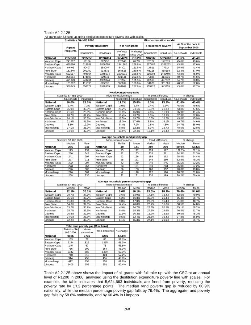
268
Table A2.2.125.
Table A2.2.125 above shows the impact of all grants with full take up, with the CSG at an annual level of R1200 in 2000, analysed using the destitution expenditure poverty line with scales. For example, the table indicates that 5,624,663 individuals are freed from poverty, reducing the poverty rate by 13.2 percentage points. The median rand poverty gap is reduced by 80.9% nationally, while the median percentage poverty gap falls by 79.4%. The aggregate rand poverty gap falls by 58.6% nationally, and by 60.4% in Limpopo.
All grants with full take-up, using destitution expenditure poverty line with scales
households individuals # of new grants
% change since 2000 households individuals households individuals
National 2656508 2205053 12394814 5664220 213.2% 916837 5624663 41.6% 45.4%Western Cape 241897 58106 287755 170948 70.7% 26127 142673 45.0% 49.6%Eastern Cape 499290 518881 2856788 1341860 268.8% 227489 1359253 43.8% 47.6%Northern Cape 69402 40407 188097 84302 121.5% 14511 77914 35.9% 41.4%Free State 131645 201959 913831 354823 269.5% 65215 338293 32.3% 37.0%KwaZulu-Natal 522017 494564 3245574 1506210 288.5% 216794 1489046 43.8% 45.9%Northwest 208084 174108 929641 421441 202.5% 70886 414531 40.7% 44.6%Gauteng 471943 249261 1309074 573558 121.5% 86518 497772 34.7% 38.0%Mpumalanga 161387 111590 685695 306269 189.8% 54070 361826 48.5% 52.8%Limpopo 350843 356177 1978359 904809 257.9% 155227 943355 43.6% 47.7%
households individuals households individuals households individuals households individualsNational 20.0% 29.0% National 11.7% 15.8% 8.3% 13.2% 41.6% 45.4%Western Cape 5.4% 7.3% Western Cape 3.0% 3.7% 2.4% 3.6% 45.0% 49.6%Eastern Cape 35.9% 45.9% Eastern Cape 20.2% 24.1% 15.8% 21.8% 43.8% 47.6%Northern Cape 21.6% 28.8% Northern Cape 13.8% 16.9% 7.8% 11.9% 35.9% 41.4%Free State 28.7% 37.7% Free State 19.4% 23.7% 9.3% 13.9% 32.3% 37.0%KwaZulu-Natal 24.1% 36.3% KwaZulu-Natal 13.5% 19.7% 10.6% 16.7% 43.8% 45.9%Northwest 21.9% 31.7% Northwest 13.0% 17.6% 8.9% 14.1% 40.7% 44.6%Gauteng 8.1% 12.7% Gauteng 5.3% 7.9% 2.8% 4.8% 34.7% 38.0%Mpumalanga 17.1% 25.9% Mpumalanga 8.8% 12.2% 8.3% 13.7% 48.5% 52.8%Limpopo 34.6% 42.8% Limpopo 19.5% 22.4% 15.1% 20.4% 43.6% 47.7%
Median Mean Median Mean Median Mean Median MeanNational 256 341 National 49 141 207 200 80.9% 58.6%Western Cape 173 234 Western Cape 25 112 224 122 129.7% 52.1%Eastern Cape 266 344 Eastern Cape 42 133 224 211 84.3% 61.3%Northern Cape 241 297 Northern Cape 52 136 189 162 78.4% 54.4%Free State 237 311 Free State 88 161 149 150 62.8% 48.3%KwaZulu-Natal 292 394 KwaZulu-Natal 42 149 249 246 85.5% 62.3%Northwest 273 354 Northwest 63 151 210 203 76.9% 57.2%Gauteng 226 306 Gauteng 66 153 160 152 70.8% 49.8%Mpumalanga 226 307 Mpumalanga 4 118 222 190 98.2% 61.8%Limpopo 268 330 Limpopo 32 131 236 199 88.2% 60.4%
Median Mean Median Mean Median Mean Median MeanNational 32.1% 35.1% National 6.6% 16.1% 25.5% 18.9% 79.4% 54.0%Western Cape 20.7% 27.3% Western Cape 3.6% 13.9% 17.1% 13.4% 82.6% 49.0%Eastern Cape 35.5% 37.7% Eastern Cape 5.2% 16.3% 30.3% 21.4% 85.4% 56.7%Northern Cape 31.0% 33.6% Northern Cape 9.0% 17.3% 22.0% 16.4% 71.0% 48.7%Free State 34.6% 37.6% Free State 14.4% 20.8% 20.2% 16.8% 58.5% 44.8%KwaZulu-Natal 33.2% 35.2% KwaZulu-Natal 4.9% 14.7% 28.3% 20.5% 85.1% 58.2%Northwest 35.7% 37.9% Northwest 8.4% 18.3% 27.3% 19.6% 76.5% 51.7%Gauteng 26.8% 29.8% Gauteng 10.9% 16.3% 15.9% 13.5% 59.5% 45.3%Mpumalanga 24.0% 28.8% Mpumalanga 0.5% 12.4% 23.5% 16.4% 97.8% 56.9%Limpopo 32.2% 35.3% Limpopo 5.1% 15.3% 27.1% 20.0% 84.1% 56.7%
Statistics SA I&E 2000
Micro-simulation Rand difference % change
National 9025 3739 5286 58.6%Western Cape 163 78 85 52.1%Eastern Cape 2144 829 1315 61.3%Northern Cape 145 67 78 53.8%Free State 755 390 364 48.3%KwaZulu-Natal 2342 882 1459 62.3%Northwest 740 316 424 57.2%Gauteng 914 458 455 49.8%Mpumalanga 412 158 255 61.8%Limpopo 1409 558 851 60.4%
Total rand poverty gap (R millions)
Statistics SA I&E 2000 Micro-simulation model
Micro-simulation modelStatistics SA I&E 2000
Poverty Headcount# grant
recipients
% point differenceAverage household percentage poverty gap
Average household rand poverty gap% change
% changeMicro-simulation model
% change
Headcount poverty rates
# of new grants # freed from poverty As % of the poor in September 2000
Statistics SA I&E 2000 % point difference
Statistics SA I&E 2000 Micro-simulation model Rand difference

269
Table A2.2.126.
Table A2.2.126 above shows the impact of all grants with full take up, with the CSG at an annual level of R1606 in 2000, analysed using the destitution expenditure poverty line with scales. For example, the table indicates that 6,837,195 individuals are freed from poverty, reducing the poverty rate by 16.0 percentage points. The median rand poverty gap is reduced by 98.8% nationally, while the median percentage poverty gap falls by 98.6%. The aggregate rand poverty gap falls by 66.6% nationally, and by 69.2% in Limpopo.
All grants(1606) with full take-up, using destitution expenditure poverty line with scales
households individuals # of new grants
% change since 2000 households individuals households individuals
National 2656508 2205053 12394814 5664220 213.2% 1090127 6837195 49.4% 55.2%Western Cape 241897 58106 287755 170948 70.7% 30204 167184 52.0% 58.1%Eastern Cape 499290 518881 2856788 1341860 268.8% 271490 1646907 52.3% 57.6%Northern Cape 69402 40407 188097 84302 121.5% 17295 94560 42.8% 50.3%Free State 131645 201959 913831 354823 269.5% 75256 389873 37.3% 42.7%KwaZulu-Natal 522017 494564 3245574 1506210 288.5% 262398 1858260 53.1% 57.3%Northwest 208084 174108 929641 421441 202.5% 81790 486516 47.0% 52.3%Gauteng 471943 249261 1309074 573558 121.5% 103811 622735 41.6% 47.6%Mpumalanga 161387 111590 685695 306269 189.8% 65402 445340 58.6% 64.9%Limpopo 350843 356177 1978359 904809 257.9% 182481 1125820 51.2% 56.9%
households individuals households individuals households individuals households individualsNational 20.0% 29.0% National 10.1% 13.0% 9.9% 16.0% 49.4% 55.2%Western Cape 5.4% 7.3% Western Cape 2.6% 3.0% 2.8% 4.2% 52.0% 58.1%Eastern Cape 35.9% 45.9% Eastern Cape 17.1% 19.4% 18.8% 26.5% 52.3% 57.6%Northern Cape 21.6% 28.8% Northern Cape 12.3% 14.3% 9.2% 14.5% 42.8% 50.3%Free State 28.7% 37.7% Free State 18.0% 21.6% 10.7% 16.1% 37.3% 42.7%KwaZulu-Natal 24.1% 36.3% KwaZulu-Natal 11.3% 15.5% 12.8% 20.8% 53.1% 57.3%Northwest 21.9% 31.7% Northwest 11.6% 15.1% 10.3% 16.6% 47.0% 52.3%Gauteng 8.1% 12.7% Gauteng 4.7% 6.7% 3.4% 6.0% 41.6% 47.6%Mpumalanga 17.1% 25.9% Mpumalanga 7.1% 9.1% 10.0% 16.8% 58.6% 64.9%Limpopo 34.6% 42.8% Limpopo 16.9% 18.5% 17.7% 24.4% 51.2% 56.9%
Median Mean Median Mean Median Mean Median MeanNational 256 341 National 3 114 253 227 98.8% 66.6%Western Cape 173 234 Western Cape 0 96 266 138 153.8% 58.9%Eastern Cape 266 344 Eastern Cape 0 106 266 238 100.0% 69.2%Northern Cape 241 297 Northern Cape 37 116 204 181 84.7% 60.8%Free State 237 311 Free State 62 139 175 173 73.9% 55.4%KwaZulu-Natal 292 394 KwaZulu-Natal 0 114 292 280 100.0% 71.0%Northwest 273 354 Northwest 21 125 252 230 92.5% 64.8%Gauteng 226 306 Gauteng 50 132 176 174 77.9% 56.9%Mpumalanga 226 307 Mpumalanga 0 94 226 213 100.0% 69.4%Limpopo 268 330 Limpopo 0 102 268 228 100.0% 69.2%
Median Mean Median Mean Median Mean Median MeanNational 32.1% 35.1% National 0.4% 13.6% 31.7% 21.4% 98.6% 61.1%Western Cape 20.7% 27.3% Western Cape 0.0% 12.2% 20.7% 15.1% 100.0% 55.2%Eastern Cape 35.5% 37.7% Eastern Cape 0.0% 13.7% 35.5% 24.0% 100.0% 63.7%Northern Cape 31.0% 33.6% Northern Cape 6.5% 15.3% 24.5% 18.3% 79.0% 54.4%Free State 34.6% 37.6% Free State 9.1% 18.3% 25.4% 19.3% 73.6% 51.4%KwaZulu-Natal 33.2% 35.2% KwaZulu-Natal 0.0% 12.0% 33.2% 23.2% 100.0% 65.8%Northwest 35.7% 37.9% Northwest 2.6% 15.8% 33.1% 22.1% 92.6% 58.4%Gauteng 26.8% 29.8% Gauteng 6.1% 14.4% 20.7% 15.4% 77.4% 51.6%Mpumalanga 24.0% 28.8% Mpumalanga 0.0% 10.4% 24.0% 18.4% 100.0% 63.8%Limpopo 32.2% 35.3% Limpopo 0.0% 12.5% 32.2% 22.8% 100.0% 64.7%
Statistics SA I&E 2000
Micro-simulation Rand difference % change
National 9025 3017 6008 66.6%Western Cape 163 67 96 58.9%Eastern Cape 2144 661 1483 69.2%Northern Cape 145 57 87 60.3%Free State 755 336 418 55.4%KwaZulu-Natal 2342 679 1662 71.0%Northwest 740 260 480 64.8%Gauteng 914 394 520 56.9%Mpumalanga 412 126 286 69.4%Limpopo 1409 434 975 69.2%
% change
Headcount poverty rates
# of new grants # freed from poverty As % of the poor in September 2000
Statistics SA I&E 2000 % point difference
Statistics SA I&E 2000 Micro-simulation model Rand differenceAverage household rand poverty gap
% change
% changeMicro-simulation model
Total rand poverty gap (R millions)
Statistics SA I&E 2000 Micro-simulation model
Micro-simulation modelStatistics SA I&E 2000
Poverty Headcount# grant
recipients
% point differenceAverage household percentage poverty gap
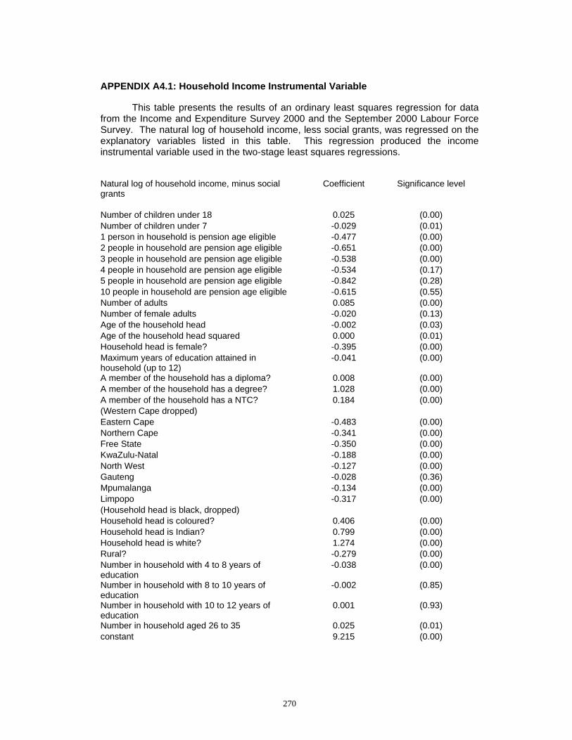
270
APPENDIX A4.1: Household Income Instrumental Variable
This table presents the results of an ordinary least squares regression for data from the Income and Expenditure Survey 2000 and the September 2000 Labour Force Survey. The natural log of household income, less social grants, was regressed on the explanatory variables listed in this table. This regression produced the income instrumental variable used in the two-stage least squares regressions.
Natural log of household income, minus social grants
Coefficient Significance level
Number of children under 18 0.025 (0.00) Number of children under 7 -0.029 (0.01) 1 person in household is pension age eligible -0.477 (0.00) 2 people in household are pension age eligible -0.651 (0.00) 3 people in household are pension age eligible -0.538 (0.00) 4 people in household are pension age eligible -0.534 (0.17) 5 people in household are pension age eligible -0.842 (0.28) 10 people in household are pension age eligible -0.615 (0.55) Number of adults 0.085 (0.00) Number of female adults -0.020 (0.13) Age of the household head -0.002 (0.03) Age of the household head squared 0.000 (0.01) Household head is female? -0.395 (0.00) Maximum years of education attained in household (up to 12)
-0.041 (0.00)
A member of the household has a diploma? 0.008 (0.00) A member of the household has a degree? 1.028 (0.00) A member of the household has a NTC? 0.184 (0.00) (Western Cape dropped) Eastern Cape -0.483 (0.00) Northern Cape -0.341 (0.00) Free State -0.350 (0.00) KwaZulu-Natal -0.188 (0.00) North West -0.127 (0.00) Gauteng -0.028 (0.36) Mpumalanga -0.134 (0.00) Limpopo -0.317 (0.00) (Household head is black, dropped) Household head is coloured? 0.406 (0.00) Household head is Indian? 0.799 (0.00) Household head is white? 1.274 (0.00) Rural? -0.279 (0.00) Number in household with 4 to 8 years of education
-0.038 (0.00)
Number in household with 8 to 10 years of education
-0.002 (0.85)
Number in household with 10 to 12 years of education
0.001 (0.93)
Number in household aged 26 to 35 0.025 (0.01) constant 9.215 (0.00)
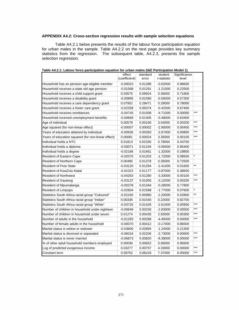
271
APPENDIX A4.2: Cross-section regression results with sample selection equations
Table A4.2.1 below presents the results of the labour force participation equation for urban males in the sample. Table A4.2.2 on the next page provides key summary statistics from the regression. The subsequent table, A4.2.3, presents the sample selection regression. Table A4.2.1: Labour force participation equation for urban males (I&E Participation Model 1)
effect (coefficient)
standard error
student t-statistic
Significance level
Household has an pension age-eligible member -0.00023 0.01288 -0.02000 0.98600 Household receives a state old age pension -0.01568 0.01291 -1.21000 0.22500 Household receives a child support grant 0.03575 0.09924 0.36000 0.71900 Household receives a disability grant -0.00895 0.01590 -0.56000 0.57300 Household receives a care dependency grant 0.07952 0.28471 0.28000 0.78000 Household receives a foster care grant -0.02258 0.05374 -0.42000 0.67400 Household receives remittances -0.04745 0.01008 -4.71000 0.00000 *** Household received unemployment benefits -0.00669 0.01405 -0.48000 0.63400 Age of individual 0.00578 0.00190 3.04000 0.00200 *** Age squared (for non-linear effect) -0.00007 0.00002 -2.90000 0.00400 *** Years of education attained by individual -0.00936 0.00350 -2.67000 0.00800 *** Years of education squared (for non-linear effect) 0.00081 0.00024 3.35000 0.00100 *** Individual holds a NTC 0.01813 0.02335 0.78000 0.43700 Individual holds a diploma -0.00071 0.01245 -0.06000 0.95400 Individual holds a degree -0.02186 0.01661 -1.32000 0.18800 Resident of Eastern Cape -0.02070 0.01203 -1.72000 0.08500 * Resident of Northern Cape 0.00485 0.01378 0.35000 0.72500 Resident of Free State -0.03120 0.01294 -2.41000 0.01600 ** Resident of KwaZulu-Natal -0.01022 0.01177 -0.87000 0.38500 Resident of Northwest -0.04263 0.01280 -3.33000 0.00100 *** Resident of Gauteng -0.03137 0.01005 -3.12000 0.00200 *** Resident of Mpumalanga -0.00378 0.01344 -0.28000 0.77800 Resident of Limpopo -0.02834 0.01598 -1.77000 0.07600 * Statistics South Africa racial group "Coloured" -0.02160 0.00980 -2.20000 0.02800 ** Statistics South Africa racial group "Indian" 0.00336 0.01540 0.22000 0.82700 Statistics South Africa racial group "White" -0.03725 0.01426 -2.61000 0.00900 *** Number of children in household under eighteen -0.00649 0.00230 -2.83000 0.00500 *** Number of children in household under seven 0.01274 0.00435 2.93000 0.00300 *** Number of adults in the household -0.01283 0.00288 -4.45000 0.00000 *** Number of female adults in the household -0.00070 0.00412 -0.17000 0.86500 Marital status is widow or widower -0.03600 0.02894 -1.24000 0.21300 Marital status is divorced or separated -0.06016 0.02206 -2.73000 0.00600 *** Marital status is never married -0.06873 0.00820 -8.38000 0.00000 *** % of other adult household members employed 0.00036 0.00652 0.06000 0.95600 Log of predicted exogenous income 0.03277 0.00757 4.33000 0.00000 *** Constant term 0.59752 0.08103 7.37000 0.00000 ***

272
Table A4.2.2: I&E Participation Model 1 summary statistics Number of observations 10836Censored observations 1094Uncensored observations 9742Wald chi-squared statistic 638.90Significance of statistic 99.9%Log likelihood -3463.09
Table A4.2.3: Selection equation for labour force participation model for urban males (I&E Participation Model 1)
effect (coefficient)
standard error
student t-statistic
significance level
Household has an pension age-eligible member 0.02572 0.07639 0.34000 0.73600 Household receives a state old age pension -0.32461 0.07224 -4.49000 0.00000 *** Household receives a child support grant 6.19645 36102.2 0.00000 1.00000 Household receives a disability grant -1.08934 0.06151 -17.71000 0.00000 *** Household receives a care dependency grant 0.51280 122020.4 0.00000 1.00000 Household receives a foster care grant 0.35582 0.36451 0.98000 0.32900 Household receives remittances -0.21484 0.06334 -3.39000 0.00100 *** Household received unemployment benefits -0.22395 0.09229 -2.43000 0.01500 ** Age of individual 0.12420 0.01068 11.63000 0.00000 *** Age squared (for non-linear effect) -0.00198 0.00013 -15.63000 0.00000 *** Years of education attained by individual 0.01190 0.01975 0.60000 0.54700 Years of education squared (for non-linear effect) 0.00230 0.00149 1.54000 0.12300 Individual holds a NTC -0.02840 0.16892 -0.17000 0.86600 Individual holds a diploma 0.34389 0.10915 3.15000 0.00200 *** Individual holds a degree 0.40110 0.14116 2.84000 0.00400 *** Resident of Eastern Cape -0.03211 0.07909 -0.41000 0.68500 Resident of Northern Cape -0.03008 0.08672 -0.35000 0.72900 Resident of Free State 0.01883 0.08902 0.21000 0.83200 Resident of KwaZulu-Natal 0.06037 0.08282 0.73000 0.46600 Resident of Northwest -0.09855 0.08643 -1.14000 0.25400 Resident of Gauteng 0.14905 0.07167 2.08000 0.03800 ** Resident of Mpumalanga 0.17406 0.09740 1.79000 0.07400 * Resident of Limpopo -0.12826 0.10986 -1.17000 0.24300 Statistics South Africa racial group "Coloured" -0.07673 0.06527 -1.18000 0.24000 Statistics South Africa racial group "Indian" -0.10244 0.10927 -0.94000 0.34900 Statistics South Africa racial group "White" -0.13244 0.09875 -1.34000 0.18000 Number of children in household under eighteen -0.00597 0.01585 -0.38000 0.70600 Number of children in household under seven 0.01220 0.03076 0.40000 0.69200 Number of adults in the household 0.00199 0.01914 0.10000 0.91700 Number of female adults in the household -0.00573 0.02660 -0.22000 0.83000 Marital status is widow or widower -0.33394 0.13757 -2.43000 0.01500 ** Marital status is divorced or separated -0.49483 0.12079 -4.10000 0.00000 *** Marital status is never married -0.49435 0.05849 -8.45000 0.00000 *** % of other adult household members employed -0.00537 0.04864 -0.11000 0.91200 Log of predicted exogenous income -0.08780 0.04911 -1.79000 0.07400 * Constant term 0.74446 0.52002 1.43000 0.15200
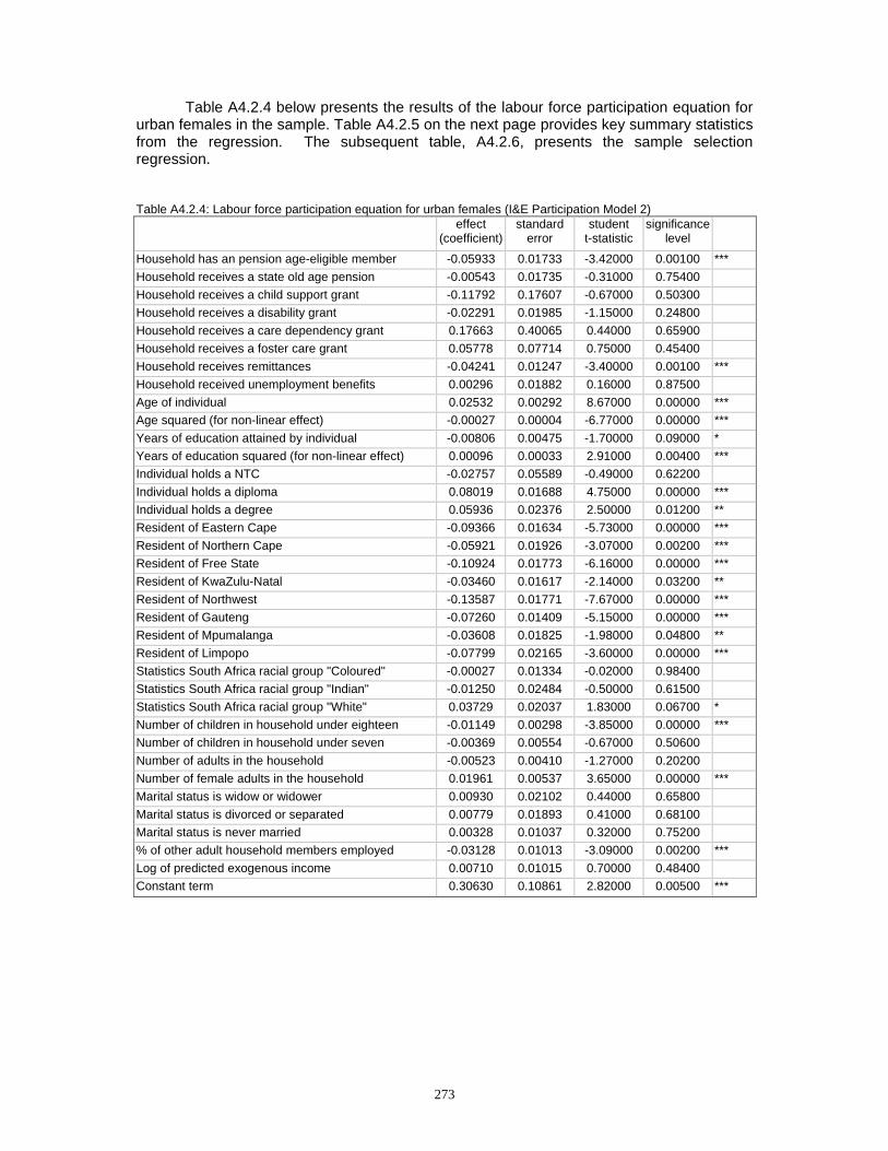
273
Table A4.2.4 below presents the results of the labour force participation equation for urban females in the sample. Table A4.2.5 on the next page provides key summary statistics from the regression. The subsequent table, A4.2.6, presents the sample selection regression. Table A4.2.4: Labour force participation equation for urban females (I&E Participation Model 2)
effect (coefficient)
standard error
student t-statistic
significance level
Household has an pension age-eligible member -0.05933 0.01733 -3.42000 0.00100 *** Household receives a state old age pension -0.00543 0.01735 -0.31000 0.75400 Household receives a child support grant -0.11792 0.17607 -0.67000 0.50300 Household receives a disability grant -0.02291 0.01985 -1.15000 0.24800 Household receives a care dependency grant 0.17663 0.40065 0.44000 0.65900 Household receives a foster care grant 0.05778 0.07714 0.75000 0.45400 Household receives remittances -0.04241 0.01247 -3.40000 0.00100 *** Household received unemployment benefits 0.00296 0.01882 0.16000 0.87500 Age of individual 0.02532 0.00292 8.67000 0.00000 *** Age squared (for non-linear effect) -0.00027 0.00004 -6.77000 0.00000 *** Years of education attained by individual -0.00806 0.00475 -1.70000 0.09000 * Years of education squared (for non-linear effect) 0.00096 0.00033 2.91000 0.00400 *** Individual holds a NTC -0.02757 0.05589 -0.49000 0.62200 Individual holds a diploma 0.08019 0.01688 4.75000 0.00000 *** Individual holds a degree 0.05936 0.02376 2.50000 0.01200 ** Resident of Eastern Cape -0.09366 0.01634 -5.73000 0.00000 *** Resident of Northern Cape -0.05921 0.01926 -3.07000 0.00200 *** Resident of Free State -0.10924 0.01773 -6.16000 0.00000 *** Resident of KwaZulu-Natal -0.03460 0.01617 -2.14000 0.03200 ** Resident of Northwest -0.13587 0.01771 -7.67000 0.00000 *** Resident of Gauteng -0.07260 0.01409 -5.15000 0.00000 *** Resident of Mpumalanga -0.03608 0.01825 -1.98000 0.04800 ** Resident of Limpopo -0.07799 0.02165 -3.60000 0.00000 *** Statistics South Africa racial group "Coloured" -0.00027 0.01334 -0.02000 0.98400 Statistics South Africa racial group "Indian" -0.01250 0.02484 -0.50000 0.61500 Statistics South Africa racial group "White" 0.03729 0.02037 1.83000 0.06700 * Number of children in household under eighteen -0.01149 0.00298 -3.85000 0.00000 *** Number of children in household under seven -0.00369 0.00554 -0.67000 0.50600 Number of adults in the household -0.00523 0.00410 -1.27000 0.20200 Number of female adults in the household 0.01961 0.00537 3.65000 0.00000 *** Marital status is widow or widower 0.00930 0.02102 0.44000 0.65800 Marital status is divorced or separated 0.00779 0.01893 0.41000 0.68100 Marital status is never married 0.00328 0.01037 0.32000 0.75200 % of other adult household members employed -0.03128 0.01013 -3.09000 0.00200 *** Log of predicted exogenous income 0.00710 0.01015 0.70000 0.48400 Constant term 0.30630 0.10861 2.82000 0.00500 ***

274
Table A4.2.5: I&E Participation Model 2 summary statistics Number of observations 11665Censored observations 2248Uncensored observations 9417Wald chi-squared statistic 614.71Significance of statistic 99.9%Log likelihood -8258.13
Table A4.2.6: Selection equation for labour force participation model for urban females (I&E Participation Model 2)
effect (coefficient)
standard error
student t-statistic
significance level
Household has an pension age-eligible member 0.03155 0.06743 0.47000 0.64000 Household receives a state old age pension -0.27584 0.06492 -4.25000 0.00000 *** Household receives a child support grant 0.07572 0.63472 0.12000 0.90500 Household receives a disability grant -0.73782 0.05608 -13.16000 0.00000 *** Household receives a care dependency grant 7.32170 236935.3 0.00000 1.00000 Household receives a foster care grant -0.17305 0.26550 -0.65000 0.51500 Household receives remittances -0.08179 0.05114 -1.60000 0.11000 Household received unemployment benefits -0.01732 0.07781 -0.22000 0.82400 Age of individual 0.11483 0.01020 11.26000 0.00000 *** Age squared (for non-linear effect) -0.00177 0.00013 -13.60000 0.00000 *** Years of education attained by individual -0.00692 0.01610 -0.43000 0.66700 Years of education squared (for non-linear effect) 0.00500 0.00120 4.16000 0.00000 *** Individual holds a NTC 0.49351 0.35276 1.40000 0.16200 Individual holds a diploma 0.63428 0.07767 8.17000 0.00000 *** Individual holds a degree 0.89864 0.11186 8.03000 0.00000 *** Resident of Eastern Cape 0.00711 0.06405 0.11000 0.91200 Resident of Northern Cape -0.19449 0.06726 -2.89000 0.00400 *** Resident of Free State 0.11771 0.07086 1.66000 0.09700 * Resident of KwaZulu-Natal -0.00588 0.06405 -0.09000 0.92700 Resident of Northwest -0.12463 0.06802 -1.83000 0.06700 * Resident of Gauteng 0.12367 0.05596 2.21000 0.02700 ** Resident of Mpumalanga 0.13483 0.07407 1.82000 0.06900 * Resident of Limpopo 0.14241 0.09230 1.54000 0.12300 Statistics South Africa racial group "Coloured" -0.11619 0.05069 -2.29000 0.02200 ** Statistics South Africa racial group "Indian" -0.64957 0.07872 -8.25000 0.00000 *** Statistics South Africa racial group "White" -0.35017 0.07516 -4.66000 0.00000 *** Number of children in household under eighteen -0.01659 0.01202 -1.38000 0.16800 Number of children in household under seven -0.03233 0.02221 -1.46000 0.14600 Number of adults in the household 0.01662 0.01660 1.00000 0.31700 Number of female adults in the household 0.00342 0.02288 0.15000 0.88100 Marital status is widow or widower 0.10957 0.06902 1.59000 0.11200 Marital status is divorced or separated 0.53334 0.08152 6.54000 0.00000 *** Marital status is never married 0.35866 0.04257 8.43000 0.00000 *** % of other adult household members employed -0.17820 0.04179 -4.26000 0.00000 *** Log of predicted exogenous income -0.19917 0.03758 -5.30000 0.00000 *** Constant term 0.92641 0.40596 2.28000 0.02200 **
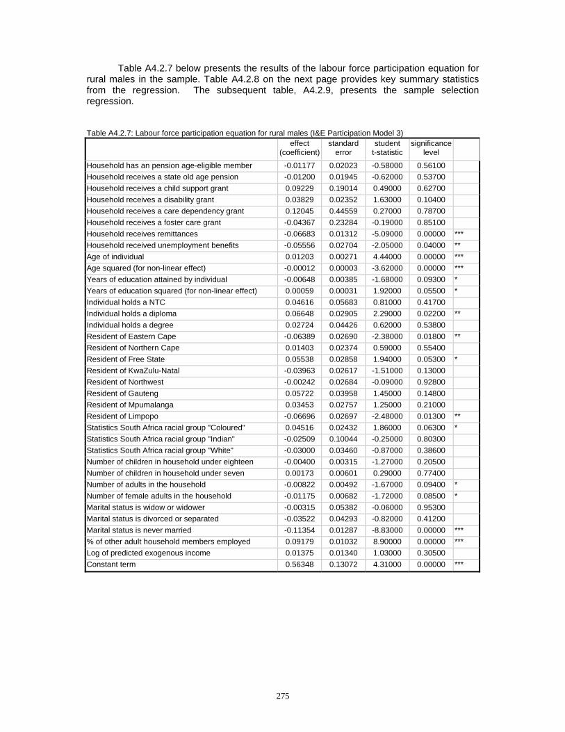
275
Table A4.2.7 below presents the results of the labour force participation equation for rural males in the sample. Table A4.2.8 on the next page provides key summary statistics from the regression. The subsequent table, A4.2.9, presents the sample selection regression. Table A4.2.7: Labour force participation equation for rural males (I&E Participation Model 3)
effect (coefficient)
standard error
student t-statistic
significance level
Household has an pension age-eligible member -0.01177 0.02023 -0.58000 0.56100 Household receives a state old age pension -0.01200 0.01945 -0.62000 0.53700 Household receives a child support grant 0.09229 0.19014 0.49000 0.62700 Household receives a disability grant 0.03829 0.02352 1.63000 0.10400 Household receives a care dependency grant 0.12045 0.44559 0.27000 0.78700 Household receives a foster care grant -0.04367 0.23284 -0.19000 0.85100 Household receives remittances -0.06683 0.01312 -5.09000 0.00000 *** Household received unemployment benefits -0.05556 0.02704 -2.05000 0.04000 ** Age of individual 0.01203 0.00271 4.44000 0.00000 *** Age squared (for non-linear effect) -0.00012 0.00003 -3.62000 0.00000 *** Years of education attained by individual -0.00648 0.00385 -1.68000 0.09300 * Years of education squared (for non-linear effect) 0.00059 0.00031 1.92000 0.05500 * Individual holds a NTC 0.04616 0.05683 0.81000 0.41700 Individual holds a diploma 0.06648 0.02905 2.29000 0.02200 ** Individual holds a degree 0.02724 0.04426 0.62000 0.53800 Resident of Eastern Cape -0.06389 0.02690 -2.38000 0.01800 ** Resident of Northern Cape 0.01403 0.02374 0.59000 0.55400 Resident of Free State 0.05538 0.02858 1.94000 0.05300 * Resident of KwaZulu-Natal -0.03963 0.02617 -1.51000 0.13000 Resident of Northwest -0.00242 0.02684 -0.09000 0.92800 Resident of Gauteng 0.05722 0.03958 1.45000 0.14800 Resident of Mpumalanga 0.03453 0.02757 1.25000 0.21000 Resident of Limpopo -0.06696 0.02697 -2.48000 0.01300 ** Statistics South Africa racial group "Coloured" 0.04516 0.02432 1.86000 0.06300 * Statistics South Africa racial group "Indian" -0.02509 0.10044 -0.25000 0.80300 Statistics South Africa racial group "White" -0.03000 0.03460 -0.87000 0.38600 Number of children in household under eighteen -0.00400 0.00315 -1.27000 0.20500 Number of children in household under seven 0.00173 0.00601 0.29000 0.77400 Number of adults in the household -0.00822 0.00492 -1.67000 0.09400 * Number of female adults in the household -0.01175 0.00682 -1.72000 0.08500 * Marital status is widow or widower -0.00315 0.05382 -0.06000 0.95300 Marital status is divorced or separated -0.03522 0.04293 -0.82000 0.41200 Marital status is never married -0.11354 0.01287 -8.83000 0.00000 *** % of other adult household members employed 0.09179 0.01032 8.90000 0.00000 *** Log of predicted exogenous income 0.01375 0.01340 1.03000 0.30500 Constant term 0.56348 0.13072 4.31000 0.00000 ***

276
Table A4.2.8 I&E Participation Model 3 summary statistics Number of observations 6788Censored observations 805Uncensored observations 5983Wald chi-squared statistic 916.17Significance of statistic 99.9%Log likelihood -3779.78
Table A4.2.9: Selection equation for labour force participation model for rural males (I&E Participation Model 3)
effect (coefficient)
standard error
student t-statistic
significance level
Household has an pension age-eligible member 0.06328 0.09001 0.70000 0.48200 Household receives a state old age pension -0.42774 0.08123 -5.27000 0.00000 *** Household receives a child support grant 6.80054 751315.6 0.00000 1.00000 Household receives a disability grant -0.93256 0.07411 -12.58000 0.00000 *** Household receives a care dependency grant 1.91760 1286249.0 0.00000 1.00000 Household receives a foster care grant -1.14644 1.00647 -1.14000 0.25500 Household receives remittances -0.23180 0.06076 -3.82000 0.00000 *** Household received unemployment benefits -0.09728 0.13944 -0.70000 0.48500 Age of individual 0.07335 0.01231 5.96000 0.00000 *** Age squared (for non-linear effect) -0.00129 0.00015 -8.86000 0.00000 *** Years of education attained by individual 0.06389 0.01825 3.50000 0.00000 *** Years of education squared (for non-linear effect) -0.00104 0.00158 -0.66000 0.50900 Individual holds a NTC 0.46965 0.47712 0.98000 0.32500 Individual holds a diploma 0.43017 0.22081 1.95000 0.05100 * Individual holds a degree 0.85629 0.46159 1.86000 0.06400 * Resident of Eastern Cape -0.52887 0.17622 -3.00000 0.00300 Resident of Northern Cape -0.18581 0.15527 -1.20000 0.23100 Resident of Free State -0.18157 0.19396 -0.94000 0.34900 Resident of KwaZulu-Natal -0.39093 0.17495 -2.23000 0.02500 ** Resident of Northwest -0.41917 0.17868 -2.35000 0.01900 ** Resident of Gauteng 0.03137 0.31359 0.10000 0.92000 Resident of Mpumalanga -0.36100 0.18260 -1.98000 0.04800 ** Resident of Limpopo -0.50866 0.17816 -2.86000 0.00400 *** Statistics South Africa racial group "Coloured" -0.01962 0.15851 -0.12000 0.90200 Statistics South Africa racial group "Indian" -0.54330 0.48140 -1.13000 0.25900 Statistics South Africa racial group "White" -0.19810 0.21020 -0.94000 0.34600 Number of children in household under eighteen -0.03276 0.01528 -2.14000 0.03200 ** Number of children in household under seven 0.05762 0.02931 1.97000 0.04900 ** Number of adults in the household 0.02930 0.02465 1.19000 0.23500 Number of female adults in the household -0.03006 0.03275 -0.92000 0.35900 Marital status is widow or widower -0.52270 0.19041 -2.75000 0.00600 *** Marital status is divorced or separated -0.89227 0.15671 -5.69000 0.00000 *** Marital status is never married -0.63518 0.06764 -9.39000 0.00000 *** % of other adult household members employed 0.14895 0.05712 2.61000 0.00900 *** Log of predicted exogenous income -0.08071 0.06575 -1.23000 0.22000 Constant term 1.77280 0.65003 2.73000 0.00600 ***
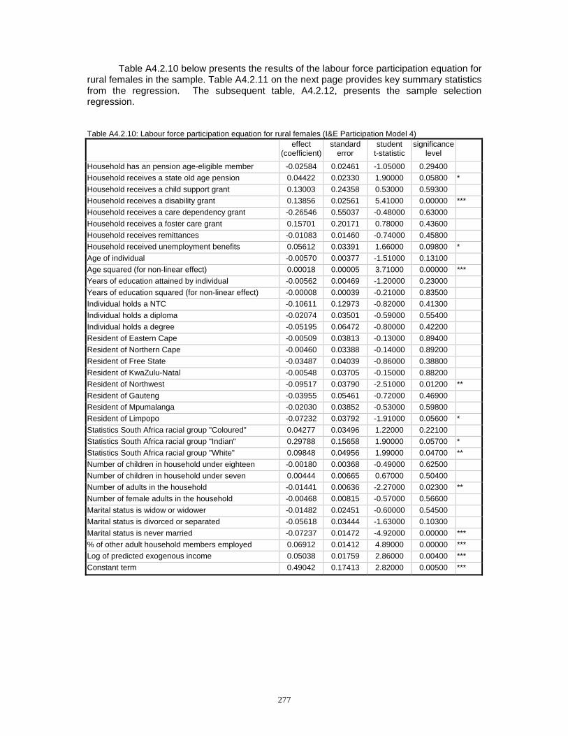
277
Table A4.2.10 below presents the results of the labour force participation equation for rural females in the sample. Table A4.2.11 on the next page provides key summary statistics from the regression. The subsequent table, A4.2.12, presents the sample selection regression. Table A4.2.10: Labour force participation equation for rural females (I&E Participation Model 4)
effect (coefficient)
standard error
student t-statistic
significance level
Household has an pension age-eligible member -0.02584 0.02461 -1.05000 0.29400 Household receives a state old age pension 0.04422 0.02330 1.90000 0.05800 * Household receives a child support grant 0.13003 0.24358 0.53000 0.59300 Household receives a disability grant 0.13856 0.02561 5.41000 0.00000 *** Household receives a care dependency grant -0.26546 0.55037 -0.48000 0.63000 Household receives a foster care grant 0.15701 0.20171 0.78000 0.43600 Household receives remittances -0.01083 0.01460 -0.74000 0.45800 Household received unemployment benefits 0.05612 0.03391 1.66000 0.09800 * Age of individual -0.00570 0.00377 -1.51000 0.13100 Age squared (for non-linear effect) 0.00018 0.00005 3.71000 0.00000 *** Years of education attained by individual -0.00562 0.00469 -1.20000 0.23000 Years of education squared (for non-linear effect) -0.00008 0.00039 -0.21000 0.83500 Individual holds a NTC -0.10611 0.12973 -0.82000 0.41300 Individual holds a diploma -0.02074 0.03501 -0.59000 0.55400 Individual holds a degree -0.05195 0.06472 -0.80000 0.42200 Resident of Eastern Cape -0.00509 0.03813 -0.13000 0.89400 Resident of Northern Cape -0.00460 0.03388 -0.14000 0.89200 Resident of Free State -0.03487 0.04039 -0.86000 0.38800 Resident of KwaZulu-Natal -0.00548 0.03705 -0.15000 0.88200 Resident of Northwest -0.09517 0.03790 -2.51000 0.01200 ** Resident of Gauteng -0.03955 0.05461 -0.72000 0.46900 Resident of Mpumalanga -0.02030 0.03852 -0.53000 0.59800 Resident of Limpopo -0.07232 0.03792 -1.91000 0.05600 * Statistics South Africa racial group "Coloured" 0.04277 0.03496 1.22000 0.22100 Statistics South Africa racial group "Indian" 0.29788 0.15658 1.90000 0.05700 * Statistics South Africa racial group "White" 0.09848 0.04956 1.99000 0.04700 ** Number of children in household under eighteen -0.00180 0.00368 -0.49000 0.62500 Number of children in household under seven 0.00444 0.00665 0.67000 0.50400 Number of adults in the household -0.01441 0.00636 -2.27000 0.02300 ** Number of female adults in the household -0.00468 0.00815 -0.57000 0.56600 Marital status is widow or widower -0.01482 0.02451 -0.60000 0.54500 Marital status is divorced or separated -0.05618 0.03444 -1.63000 0.10300 Marital status is never married -0.07237 0.01472 -4.92000 0.00000 *** % of other adult household members employed 0.06912 0.01412 4.89000 0.00000 *** Log of predicted exogenous income 0.05038 0.01759 2.86000 0.00400 *** Constant term 0.49042 0.17413 2.82000 0.00500 ***
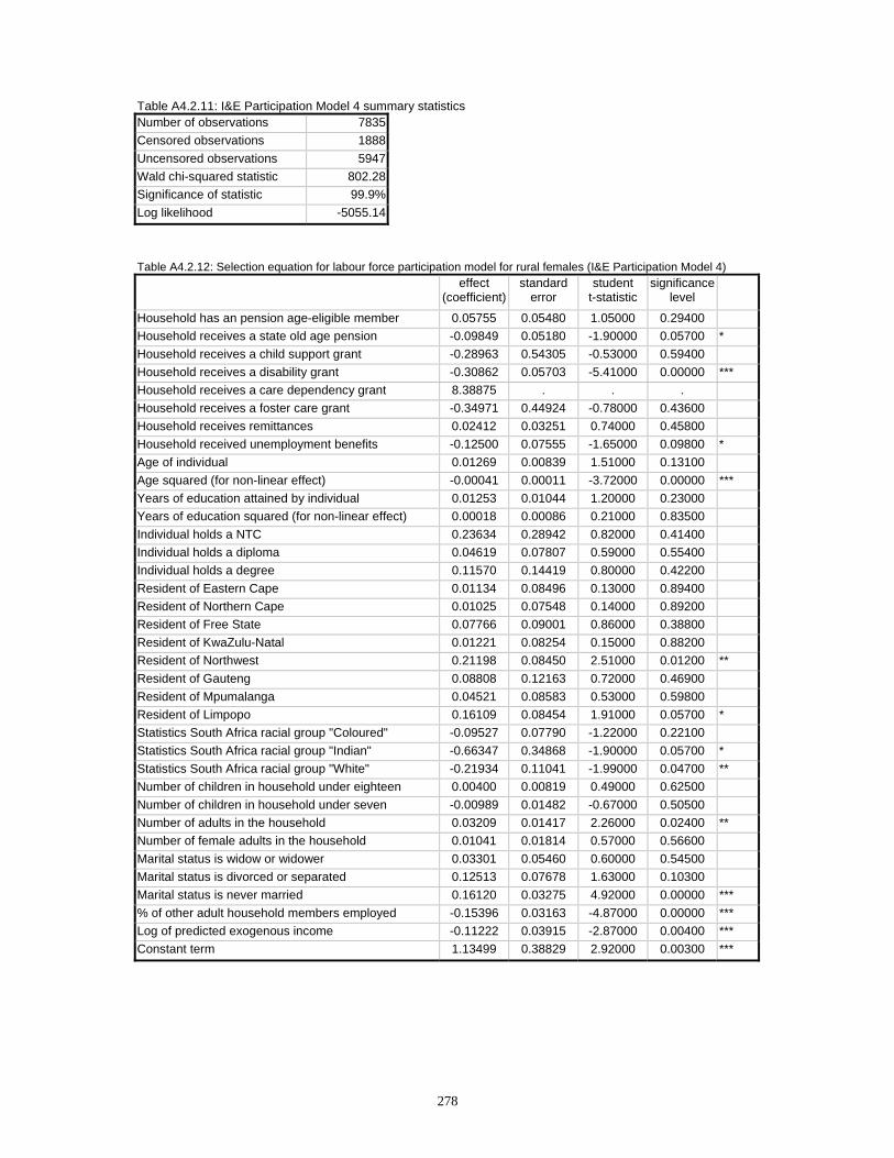
278
Table A4.2.11: I&E Participation Model 4 summary statistics Number of observations 7835Censored observations 1888Uncensored observations 5947Wald chi-squared statistic 802.28Significance of statistic 99.9%Log likelihood -5055.14
Table A4.2.12: Selection equation for labour force participation model for rural females (I&E Participation Model 4)
effect (coefficient)
standard error
student t-statistic
significance level
Household has an pension age-eligible member 0.05755 0.05480 1.05000 0.29400 Household receives a state old age pension -0.09849 0.05180 -1.90000 0.05700 * Household receives a child support grant -0.28963 0.54305 -0.53000 0.59400 Household receives a disability grant -0.30862 0.05703 -5.41000 0.00000 *** Household receives a care dependency grant 8.38875 . . . Household receives a foster care grant -0.34971 0.44924 -0.78000 0.43600 Household receives remittances 0.02412 0.03251 0.74000 0.45800 Household received unemployment benefits -0.12500 0.07555 -1.65000 0.09800 * Age of individual 0.01269 0.00839 1.51000 0.13100 Age squared (for non-linear effect) -0.00041 0.00011 -3.72000 0.00000 *** Years of education attained by individual 0.01253 0.01044 1.20000 0.23000 Years of education squared (for non-linear effect) 0.00018 0.00086 0.21000 0.83500 Individual holds a NTC 0.23634 0.28942 0.82000 0.41400 Individual holds a diploma 0.04619 0.07807 0.59000 0.55400 Individual holds a degree 0.11570 0.14419 0.80000 0.42200 Resident of Eastern Cape 0.01134 0.08496 0.13000 0.89400 Resident of Northern Cape 0.01025 0.07548 0.14000 0.89200 Resident of Free State 0.07766 0.09001 0.86000 0.38800 Resident of KwaZulu-Natal 0.01221 0.08254 0.15000 0.88200 Resident of Northwest 0.21198 0.08450 2.51000 0.01200 ** Resident of Gauteng 0.08808 0.12163 0.72000 0.46900 Resident of Mpumalanga 0.04521 0.08583 0.53000 0.59800 Resident of Limpopo 0.16109 0.08454 1.91000 0.05700 * Statistics South Africa racial group "Coloured" -0.09527 0.07790 -1.22000 0.22100 Statistics South Africa racial group "Indian" -0.66347 0.34868 -1.90000 0.05700 * Statistics South Africa racial group "White" -0.21934 0.11041 -1.99000 0.04700 ** Number of children in household under eighteen 0.00400 0.00819 0.49000 0.62500 Number of children in household under seven -0.00989 0.01482 -0.67000 0.50500 Number of adults in the household 0.03209 0.01417 2.26000 0.02400 ** Number of female adults in the household 0.01041 0.01814 0.57000 0.56600 Marital status is widow or widower 0.03301 0.05460 0.60000 0.54500 Marital status is divorced or separated 0.12513 0.07678 1.63000 0.10300 Marital status is never married 0.16120 0.03275 4.92000 0.00000 *** % of other adult household members employed -0.15396 0.03163 -4.87000 0.00000 *** Log of predicted exogenous income -0.11222 0.03915 -2.87000 0.00400 *** Constant term 1.13499 0.38829 2.92000 0.00300 ***
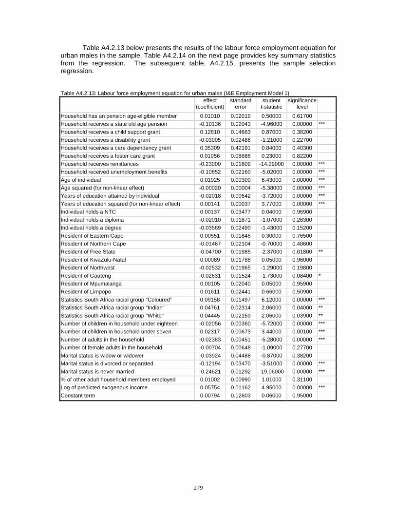
279
Table A4.2.13 below presents the results of the labour force employment equation for urban males in the sample. Table A4.2.14 on the next page provides key summary statistics from the regression. The subsequent table, A4.2.15, presents the sample selection regression. Table A4.2.13: Labour force employment equation for urban males (I&E Employment Model 1)
effect (coefficient)
standard error
student t-statistic
significance level
Household has an pension age-eligible member 0.01010 0.02019 0.50000 0.61700 Household receives a state old age pension -0.10136 0.02043 -4.96000 0.00000 *** Household receives a child support grant 0.12810 0.14663 0.87000 0.38200 Household receives a disability grant -0.03005 0.02486 -1.21000 0.22700 Household receives a care dependency grant 0.35309 0.42191 0.84000 0.40300 Household receives a foster care grant 0.01956 0.08686 0.23000 0.82200 Household receives remittances -0.23000 0.01609 -14.29000 0.00000 *** Household received unemployment benefits -0.10852 0.02160 -5.02000 0.00000 *** Age of individual 0.01925 0.00300 6.43000 0.00000 *** Age squared (for non-linear effect) -0.00020 0.00004 -5.38000 0.00000 *** Years of education attained by individual -0.02018 0.00542 -3.72000 0.00000 *** Years of education squared (for non-linear effect) 0.00141 0.00037 3.77000 0.00000 *** Individual holds a NTC 0.00137 0.03477 0.04000 0.96900 Individual holds a diploma -0.02010 0.01871 -1.07000 0.28300 Individual holds a degree -0.03569 0.02490 -1.43000 0.15200 Resident of Eastern Cape 0.00551 0.01845 0.30000 0.76500 Resident of Northern Cape -0.01467 0.02104 -0.70000 0.48600 Resident of Free State -0.04700 0.01985 -2.37000 0.01800 ** Resident of KwaZulu-Natal 0.00089 0.01788 0.05000 0.96000 Resident of Northwest -0.02532 0.01965 -1.29000 0.19800 Resident of Gauteng -0.02631 0.01524 -1.73000 0.08400 * Resident of Mpumalanga 0.00105 0.02040 0.05000 0.95900 Resident of Limpopo 0.01611 0.02441 0.66000 0.50900 Statistics South Africa racial group "Coloured" 0.09158 0.01497 6.12000 0.00000 *** Statistics South Africa racial group "Indian" 0.04761 0.02314 2.06000 0.04000 ** Statistics South Africa racial group "White" 0.04445 0.02159 2.06000 0.03900 ** Number of children in household under eighteen -0.02056 0.00360 -5.72000 0.00000 *** Number of children in household under seven 0.02317 0.00673 3.44000 0.00100 *** Number of adults in the household -0.02383 0.00451 -5.28000 0.00000 *** Number of female adults in the household -0.00704 0.00648 -1.09000 0.27700 Marital status is widow or widower -0.03924 0.04488 -0.87000 0.38200 Marital status is divorced or separated -0.12194 0.03470 -3.51000 0.00000 *** Marital status is never married -0.24621 0.01292 -19.06000 0.00000 *** % of other adult household members employed 0.01002 0.00990 1.01000 0.31100 Log of predicted exogenous income 0.05754 0.01162 4.95000 0.00000 *** Constant term 0.00794 0.12603 0.06000 0.95000
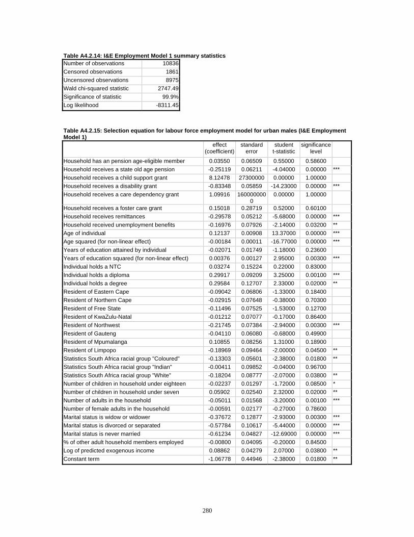
280
Table A4.2.14: I&E Employment Model 1 summary statistics Number of observations 10836Censored observations 1861Uncensored observations 8975Wald chi-squared statistic 2747.49Significance of statistic 99.9%Log likelihood -8311.45
Table A4.2.15: Selection equation for labour force employment model for urban males (I&E Employment Model 1)
effect (coefficient)
standard error
student t-statistic
significance level
Household has an pension age-eligible member 0.03550 0.06509 0.55000 0.58600 Household receives a state old age pension -0.25119 0.06211 -4.04000 0.00000 *** Household receives a child support grant 8.12478 27300000 0.00000 1.00000 Household receives a disability grant -0.83348 0.05859 -14.23000 0.00000 *** Household receives a care dependency grant 1.09916 160000000
0 0.00000 1.00000
Household receives a foster care grant 0.15018 0.28719 0.52000 0.60100 Household receives remittances -0.29578 0.05212 -5.68000 0.00000 *** Household received unemployment benefits -0.16976 0.07926 -2.14000 0.03200 ** Age of individual 0.12137 0.00908 13.37000 0.00000 *** Age squared (for non-linear effect) -0.00184 0.00011 -16.77000 0.00000 *** Years of education attained by individual -0.02071 0.01749 -1.18000 0.23600 Years of education squared (for non-linear effect) 0.00376 0.00127 2.95000 0.00300 *** Individual holds a NTC 0.03274 0.15224 0.22000 0.83000 Individual holds a diploma 0.29917 0.09209 3.25000 0.00100 *** Individual holds a degree 0.29584 0.12707 2.33000 0.02000 ** Resident of Eastern Cape -0.09042 0.06806 -1.33000 0.18400 Resident of Northern Cape -0.02915 0.07648 -0.38000 0.70300 Resident of Free State -0.11496 0.07525 -1.53000 0.12700 Resident of KwaZulu-Natal -0.01212 0.07077 -0.17000 0.86400 Resident of Northwest -0.21745 0.07384 -2.94000 0.00300 *** Resident of Gauteng -0.04110 0.06080 -0.68000 0.49900 Resident of Mpumalanga 0.10855 0.08256 1.31000 0.18900 Resident of Limpopo -0.18969 0.09464 -2.00000 0.04500 ** Statistics South Africa racial group "Coloured" -0.13303 0.05601 -2.38000 0.01800 ** Statistics South Africa racial group "Indian" -0.00411 0.09852 -0.04000 0.96700 Statistics South Africa racial group "White" -0.18204 0.08777 -2.07000 0.03800 ** Number of children in household under eighteen -0.02237 0.01297 -1.72000 0.08500 * Number of children in household under seven 0.05902 0.02540 2.32000 0.02000 ** Number of adults in the household -0.05011 0.01568 -3.20000 0.00100 *** Number of female adults in the household -0.00591 0.02177 -0.27000 0.78600 Marital status is widow or widower -0.37672 0.12877 -2.93000 0.00300 *** Marital status is divorced or separated -0.57784 0.10617 -5.44000 0.00000 *** Marital status is never married -0.61234 0.04827 -12.69000 0.00000 *** % of other adult household members employed -0.00800 0.04095 -0.20000 0.84500 Log of predicted exogenous income 0.08862 0.04279 2.07000 0.03800 ** Constant term -1.06778 0.44946 -2.38000 0.01800 **
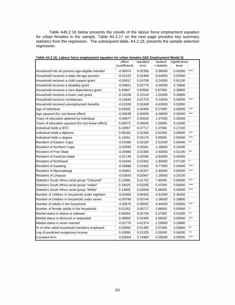
281
Table A46.2.16 below presents the results of the labour force employment equation
for urban females in the sample. Table A4.2.17 on the next page provides key summary statistics from the regression. The subsequent table, A4.2.18, presents the sample selection regression. Table A4.2.16: Labour force employment equation for urban females (I&E Employment Model 2)
effect (coefficient)
standard error
student t-statistic
significance level
Household has an pension age-eligible member -0.06974 0.02358 -2.96000 0.00300 *** Household receives a state old age pension -0.01523 0.02368 -0.64000 0.52000 Household receives a child support grant -0.05917 0.24708 -0.24000 0.81100 Household receives a disability grant -0.00821 0.02779 -0.30000 0.76800 Household receives a care dependency grant 0.43847 0.50580 0.87000 0.38600 Household receives a foster care grant -0.10338 0.10144 -1.02000 0.30800 Household receives remittances -0.15844 0.01723 -9.19000 0.00000 *** Household received unemployment benefits -0.01559 0.02469 -0.63000 0.52800 Age of individual 0.04305 0.00465 9.27000 0.00000 *** Age squared (for non-linear effect) -0.00038 0.00006 -6.06000 0.00000 *** Years of education attained by individual -0.00677 0.00632 -1.07000 0.28400 Years of education squared (for non-linear effect) 0.00073 0.00045 1.63000 0.10300 Individual holds a NTC 0.10557 0.07717 1.37000 0.17100 Individual holds a diploma 0.09183 0.02346 3.91000 0.00000 *** Individual holds a degree 0.13001 0.03176 4.09000 0.00000 *** Resident of Eastern Cape -0.04396 0.02185 -2.01000 0.04400 ** Resident of Northern Cape -0.03593 0.02581 -1.39000 0.16400 Resident of Free State -0.05980 0.02366 -2.53000 0.01100 ** Resident of KwaZulu-Natal -0.01748 0.02090 -0.84000 0.40300 Resident of Northwest -0.04444 0.02462 -1.80000 0.07100 * Resident of Gauteng -0.06888 0.01825 -3.77000 0.00000 *** Resident of Mpumalanga -0.06601 0.02357 -2.80000 0.00500 *** Resident of Limpopo -0.03643 0.02847 -1.28000 0.20100 Statistics South Africa racial group "Coloured" 0.12966 0.01752 7.40000 0.00000 *** Statistics South Africa racial group "Indian" 0.18025 0.03295 5.47000 0.00000 *** Statistics South Africa racial group "White" 0.14505 0.02608 5.56000 0.00000 *** Number of children in household under eighteen -0.00366 0.00403 -0.91000 0.36400 Number of children in household under seven -0.00789 0.00744 -1.06000 0.28800 Number of adults in the household -0.02675 0.00552 -4.84000 0.00000 *** Number of female adults in the household 0.01352 0.00717 1.88000 0.05900 * Marital status is widow or widower 0.06954 0.02706 2.57000 0.01000 ** Marital status is divorced or separated 0.08860 0.02489 3.56000 0.00000 *** Marital status is never married -0.01770 0.01374 -1.29000 0.19800 % of other adult household members employed 0.02809 0.01355 2.07000 0.03800 ** Log of predicted exogenous income 0.02695 0.01325 2.03000 0.04200 ** Constant term -0.60004 0.14984 -4.00000 0.00000 ***
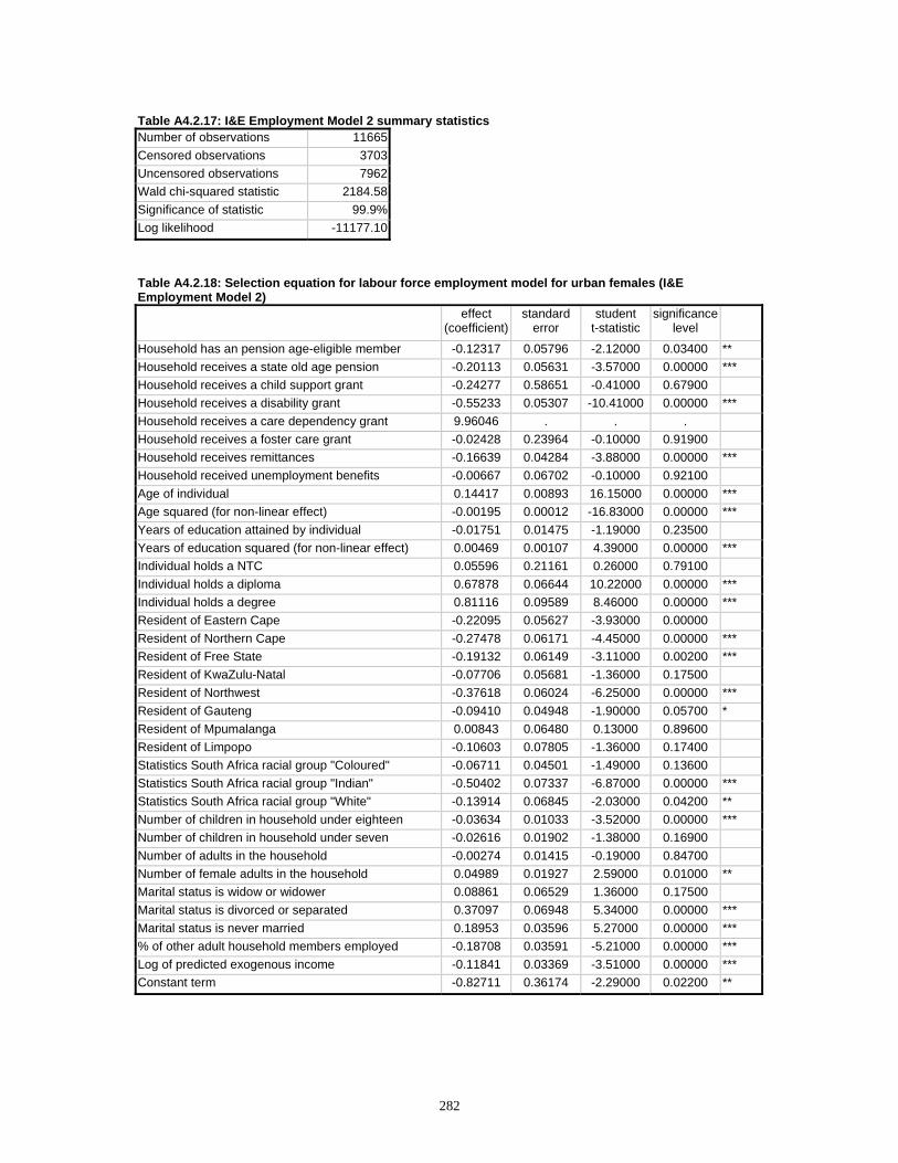
282
Table A4.2.17: I&E Employment Model 2 summary statistics Number of observations 11665Censored observations 3703Uncensored observations 7962Wald chi-squared statistic 2184.58Significance of statistic 99.9%Log likelihood -11177.10
Table A4.2.18: Selection equation for labour force employment model for urban females (I&E Employment Model 2)
effect (coefficient)
standard error
student t-statistic
significance level
Household has an pension age-eligible member -0.12317 0.05796 -2.12000 0.03400 ** Household receives a state old age pension -0.20113 0.05631 -3.57000 0.00000 *** Household receives a child support grant -0.24277 0.58651 -0.41000 0.67900 Household receives a disability grant -0.55233 0.05307 -10.41000 0.00000 *** Household receives a care dependency grant 9.96046 . . . Household receives a foster care grant -0.02428 0.23964 -0.10000 0.91900 Household receives remittances -0.16639 0.04284 -3.88000 0.00000 *** Household received unemployment benefits -0.00667 0.06702 -0.10000 0.92100 Age of individual 0.14417 0.00893 16.15000 0.00000 *** Age squared (for non-linear effect) -0.00195 0.00012 -16.83000 0.00000 *** Years of education attained by individual -0.01751 0.01475 -1.19000 0.23500 Years of education squared (for non-linear effect) 0.00469 0.00107 4.39000 0.00000 *** Individual holds a NTC 0.05596 0.21161 0.26000 0.79100 Individual holds a diploma 0.67878 0.06644 10.22000 0.00000 *** Individual holds a degree 0.81116 0.09589 8.46000 0.00000 *** Resident of Eastern Cape -0.22095 0.05627 -3.93000 0.00000 Resident of Northern Cape -0.27478 0.06171 -4.45000 0.00000 *** Resident of Free State -0.19132 0.06149 -3.11000 0.00200 *** Resident of KwaZulu-Natal -0.07706 0.05681 -1.36000 0.17500 Resident of Northwest -0.37618 0.06024 -6.25000 0.00000 *** Resident of Gauteng -0.09410 0.04948 -1.90000 0.05700 * Resident of Mpumalanga 0.00843 0.06480 0.13000 0.89600 Resident of Limpopo -0.10603 0.07805 -1.36000 0.17400 Statistics South Africa racial group "Coloured" -0.06711 0.04501 -1.49000 0.13600 Statistics South Africa racial group "Indian" -0.50402 0.07337 -6.87000 0.00000 *** Statistics South Africa racial group "White" -0.13914 0.06845 -2.03000 0.04200 ** Number of children in household under eighteen -0.03634 0.01033 -3.52000 0.00000 *** Number of children in household under seven -0.02616 0.01902 -1.38000 0.16900 Number of adults in the household -0.00274 0.01415 -0.19000 0.84700 Number of female adults in the household 0.04989 0.01927 2.59000 0.01000 ** Marital status is widow or widower 0.08861 0.06529 1.36000 0.17500 Marital status is divorced or separated 0.37097 0.06948 5.34000 0.00000 *** Marital status is never married 0.18953 0.03596 5.27000 0.00000 *** % of other adult household members employed -0.18708 0.03591 -5.21000 0.00000 *** Log of predicted exogenous income -0.11841 0.03369 -3.51000 0.00000 *** Constant term -0.82711 0.36174 -2.29000 0.02200 **

283
Table A4.2.19 below presents the results of the labour force employment equation for rural males in the sample. Table A4.2.20 on the next page provides key summary statistics from the regression. The subsequent table, A4.2.21, presents the sample selection regression. Table A4.2.19: Labour force employment equation for rural males (I&E Employment Model 3)
effect (coefficient)
standard error
student t-statistic
significance level
Household has an pension age-eligible member -0.10139 0.02491 -4.07000 0.00000 *** Household receives a state old age pension 0.09995 0.02472 4.04000 0.00000 *** Household receives a child support grant 0.02036 0.26287 0.08000 0.93800 Household receives a disability grant 0.13230 0.02718 4.87000 0.00000 *** Household receives a care dependency grant -1.28798 0.60199 -2.14000 0.03200 ** Household receives a foster care grant 0.17324 0.29661 0.58000 0.55900 Household receives remittances -0.06036 0.01751 -3.45000 0.00100 *** Household received unemployment benefits 0.01023 0.03671 0.28000 0.78000 Age of individual -0.01349 0.00327 -4.13000 0.00000 *** Age squared (for non-linear effect) 0.00022 0.00004 5.61000 0.00000 *** Years of education attained by individual 0.00040 0.00505 0.08000 0.93700 Years of education squared (for non-linear effect) -0.00098 0.00041 -2.41000 0.01600 ** Individual holds a NTC -0.16055 0.07852 -2.04000 0.04100 ** Individual holds a diploma 0.00919 0.03801 0.24000 0.80900 Individual holds a degree -0.03090 0.05825 -0.53000 0.59600 Resident of Eastern Cape -0.03850 0.03445 -1.12000 0.26400 Resident of Northern Cape -0.03000 0.03100 -0.97000 0.33300 Resident of Free State -0.07824 0.03832 -2.04000 0.04100 ** Resident of KwaZulu-Natal -0.07056 0.03510 -2.01000 0.04400 ** Resident of Northwest -0.10250 0.03630 -2.82000 0.00500 *** Resident of Gauteng -0.05192 0.05784 -0.90000 0.36900 Resident of Mpumalanga -0.10897 0.03753 -2.90000 0.00400 *** Resident of Limpopo -0.07368 0.03575 -2.06000 0.03900 ** Statistics South Africa racial group "Coloured" -0.00640 0.03410 -0.19000 0.85100 Statistics South Africa racial group "Indian" 0.21965 0.13335 1.65000 0.10000 Statistics South Africa racial group "White" 0.06999 0.04710 1.49000 0.13700 Number of children in household under eighteen -0.00024 0.00421 -0.06000 0.95500 Number of children in household under seven 0.00964 0.00801 1.20000 0.22900 Number of adults in the household -0.02058 0.00621 -3.32000 0.00100 *** Number of female adults in the household 0.01865 0.00909 2.05000 0.04000 ** Marital status is widow or widower 0.06304 0.06586 0.96000 0.33800 Marital status is divorced or separated -0.05949 0.05266 -1.13000 0.25900 Marital status is never married -0.06437 0.01638 -3.93000 0.00000 *** % of other adult household members employed 0.01833 0.01394 1.31000 0.18900 Log of predicted exogenous income 0.01888 0.00836 2.26000 0.02400 ** Constant term 1.05705 0.00076 1395.17000 0.00000 ***
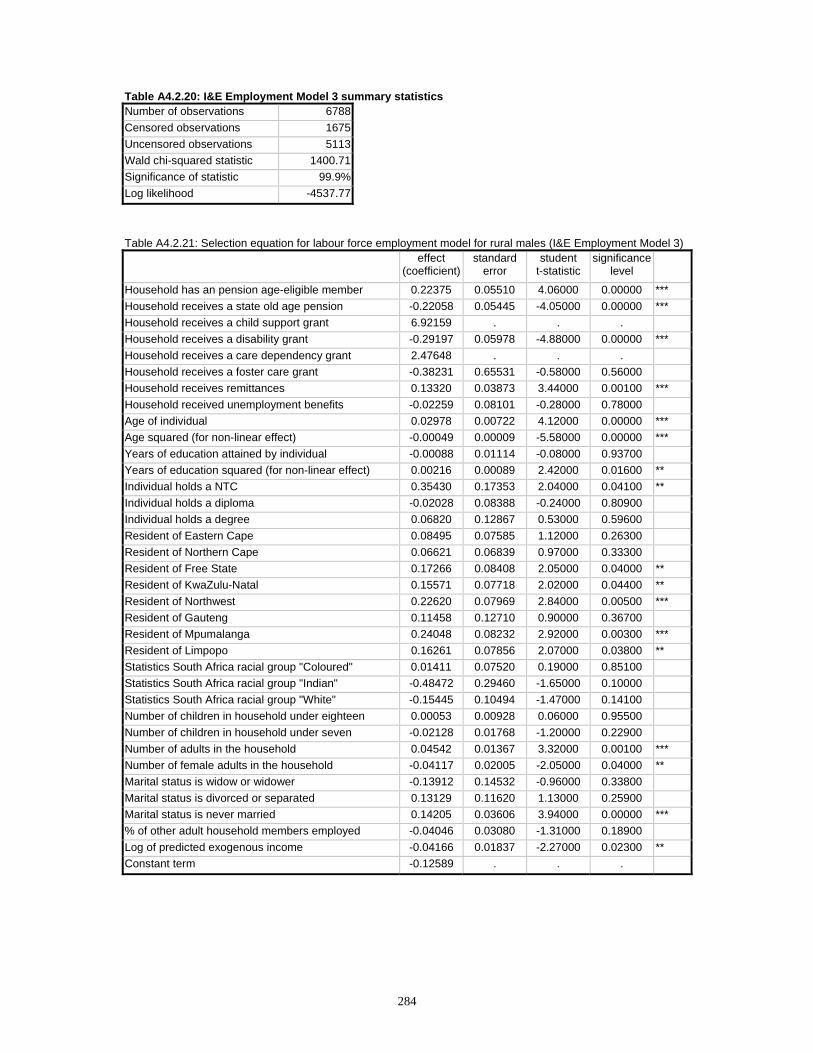
284
Table A4.2.20: I&E Employment Model 3 summary statistics Number of observations 6788Censored observations 1675Uncensored observations 5113Wald chi-squared statistic 1400.71Significance of statistic 99.9%Log likelihood -4537.77
Table A4.2.21: Selection equation for labour force employment model for rural males (I&E Employment Model 3)
effect (coefficient)
standard error
student t-statistic
significance level
Household has an pension age-eligible member 0.22375 0.05510 4.06000 0.00000 *** Household receives a state old age pension -0.22058 0.05445 -4.05000 0.00000 *** Household receives a child support grant 6.92159 . . . Household receives a disability grant -0.29197 0.05978 -4.88000 0.00000 *** Household receives a care dependency grant 2.47648 . . . Household receives a foster care grant -0.38231 0.65531 -0.58000 0.56000 Household receives remittances 0.13320 0.03873 3.44000 0.00100 *** Household received unemployment benefits -0.02259 0.08101 -0.28000 0.78000 Age of individual 0.02978 0.00722 4.12000 0.00000 *** Age squared (for non-linear effect) -0.00049 0.00009 -5.58000 0.00000 *** Years of education attained by individual -0.00088 0.01114 -0.08000 0.93700 Years of education squared (for non-linear effect) 0.00216 0.00089 2.42000 0.01600 ** Individual holds a NTC 0.35430 0.17353 2.04000 0.04100 ** Individual holds a diploma -0.02028 0.08388 -0.24000 0.80900 Individual holds a degree 0.06820 0.12867 0.53000 0.59600 Resident of Eastern Cape 0.08495 0.07585 1.12000 0.26300 Resident of Northern Cape 0.06621 0.06839 0.97000 0.33300 Resident of Free State 0.17266 0.08408 2.05000 0.04000 ** Resident of KwaZulu-Natal 0.15571 0.07718 2.02000 0.04400 ** Resident of Northwest 0.22620 0.07969 2.84000 0.00500 *** Resident of Gauteng 0.11458 0.12710 0.90000 0.36700 Resident of Mpumalanga 0.24048 0.08232 2.92000 0.00300 *** Resident of Limpopo 0.16261 0.07856 2.07000 0.03800 ** Statistics South Africa racial group "Coloured" 0.01411 0.07520 0.19000 0.85100 Statistics South Africa racial group "Indian" -0.48472 0.29460 -1.65000 0.10000 Statistics South Africa racial group "White" -0.15445 0.10494 -1.47000 0.14100 Number of children in household under eighteen 0.00053 0.00928 0.06000 0.95500 Number of children in household under seven -0.02128 0.01768 -1.20000 0.22900 Number of adults in the household 0.04542 0.01367 3.32000 0.00100 *** Number of female adults in the household -0.04117 0.02005 -2.05000 0.04000 ** Marital status is widow or widower -0.13912 0.14532 -0.96000 0.33800 Marital status is divorced or separated 0.13129 0.11620 1.13000 0.25900 Marital status is never married 0.14205 0.03606 3.94000 0.00000 *** % of other adult household members employed -0.04046 0.03080 -1.31000 0.18900 Log of predicted exogenous income -0.04166 0.01837 -2.27000 0.02300 ** Constant term -0.12589 . . .
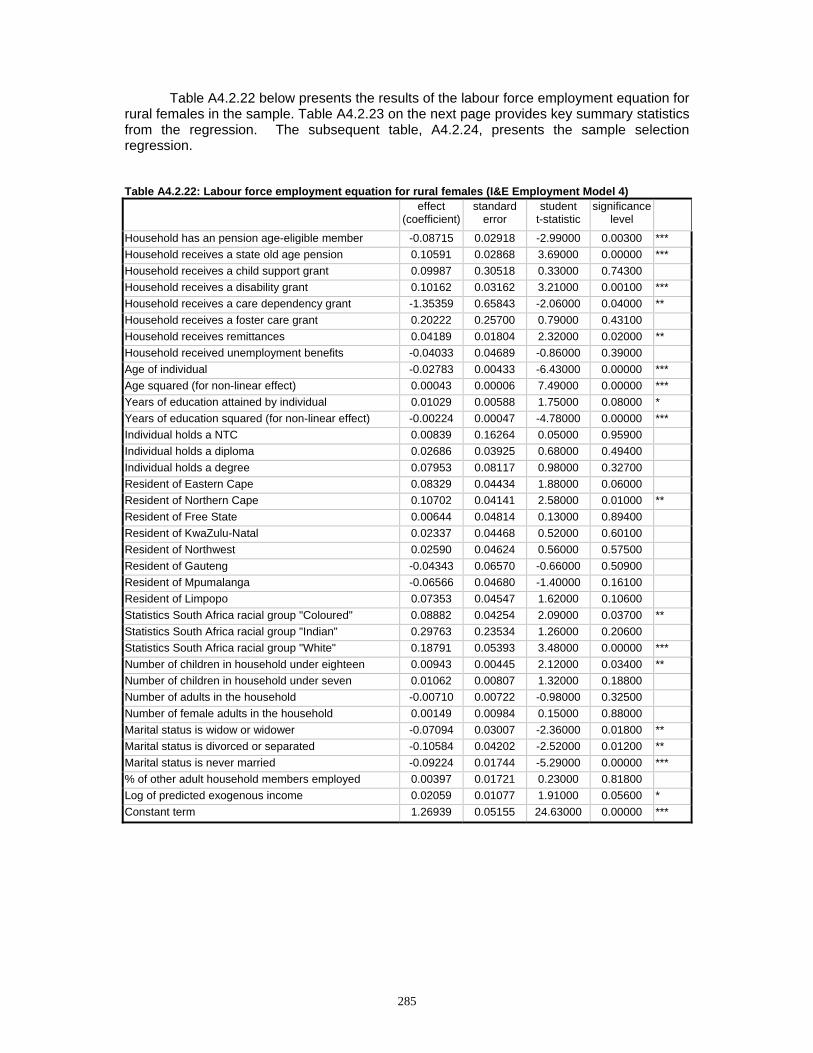
285
Table A4.2.22 below presents the results of the labour force employment equation for rural females in the sample. Table A4.2.23 on the next page provides key summary statistics from the regression. The subsequent table, A4.2.24, presents the sample selection regression. Table A4.2.22: Labour force employment equation for rural females (I&E Employment Model 4)
effect (coefficient)
standard error
student t-statistic
significance level
Household has an pension age-eligible member -0.08715 0.02918 -2.99000 0.00300 *** Household receives a state old age pension 0.10591 0.02868 3.69000 0.00000 *** Household receives a child support grant 0.09987 0.30518 0.33000 0.74300 Household receives a disability grant 0.10162 0.03162 3.21000 0.00100 *** Household receives a care dependency grant -1.35359 0.65843 -2.06000 0.04000 ** Household receives a foster care grant 0.20222 0.25700 0.79000 0.43100 Household receives remittances 0.04189 0.01804 2.32000 0.02000 ** Household received unemployment benefits -0.04033 0.04689 -0.86000 0.39000 Age of individual -0.02783 0.00433 -6.43000 0.00000 *** Age squared (for non-linear effect) 0.00043 0.00006 7.49000 0.00000 *** Years of education attained by individual 0.01029 0.00588 1.75000 0.08000 * Years of education squared (for non-linear effect) -0.00224 0.00047 -4.78000 0.00000 *** Individual holds a NTC 0.00839 0.16264 0.05000 0.95900 Individual holds a diploma 0.02686 0.03925 0.68000 0.49400 Individual holds a degree 0.07953 0.08117 0.98000 0.32700 Resident of Eastern Cape 0.08329 0.04434 1.88000 0.06000 Resident of Northern Cape 0.10702 0.04141 2.58000 0.01000 ** Resident of Free State 0.00644 0.04814 0.13000 0.89400 Resident of KwaZulu-Natal 0.02337 0.04468 0.52000 0.60100 Resident of Northwest 0.02590 0.04624 0.56000 0.57500 Resident of Gauteng -0.04343 0.06570 -0.66000 0.50900 Resident of Mpumalanga -0.06566 0.04680 -1.40000 0.16100 Resident of Limpopo 0.07353 0.04547 1.62000 0.10600 Statistics South Africa racial group "Coloured" 0.08882 0.04254 2.09000 0.03700 ** Statistics South Africa racial group "Indian" 0.29763 0.23534 1.26000 0.20600 Statistics South Africa racial group "White" 0.18791 0.05393 3.48000 0.00000 *** Number of children in household under eighteen 0.00943 0.00445 2.12000 0.03400 ** Number of children in household under seven 0.01062 0.00807 1.32000 0.18800 Number of adults in the household -0.00710 0.00722 -0.98000 0.32500 Number of female adults in the household 0.00149 0.00984 0.15000 0.88000 Marital status is widow or widower -0.07094 0.03007 -2.36000 0.01800 ** Marital status is divorced or separated -0.10584 0.04202 -2.52000 0.01200 ** Marital status is never married -0.09224 0.01744 -5.29000 0.00000 *** % of other adult household members employed 0.00397 0.01721 0.23000 0.81800 Log of predicted exogenous income 0.02059 0.01077 1.91000 0.05600 * Constant term 1.26939 0.05155 24.63000 0.00000 ***
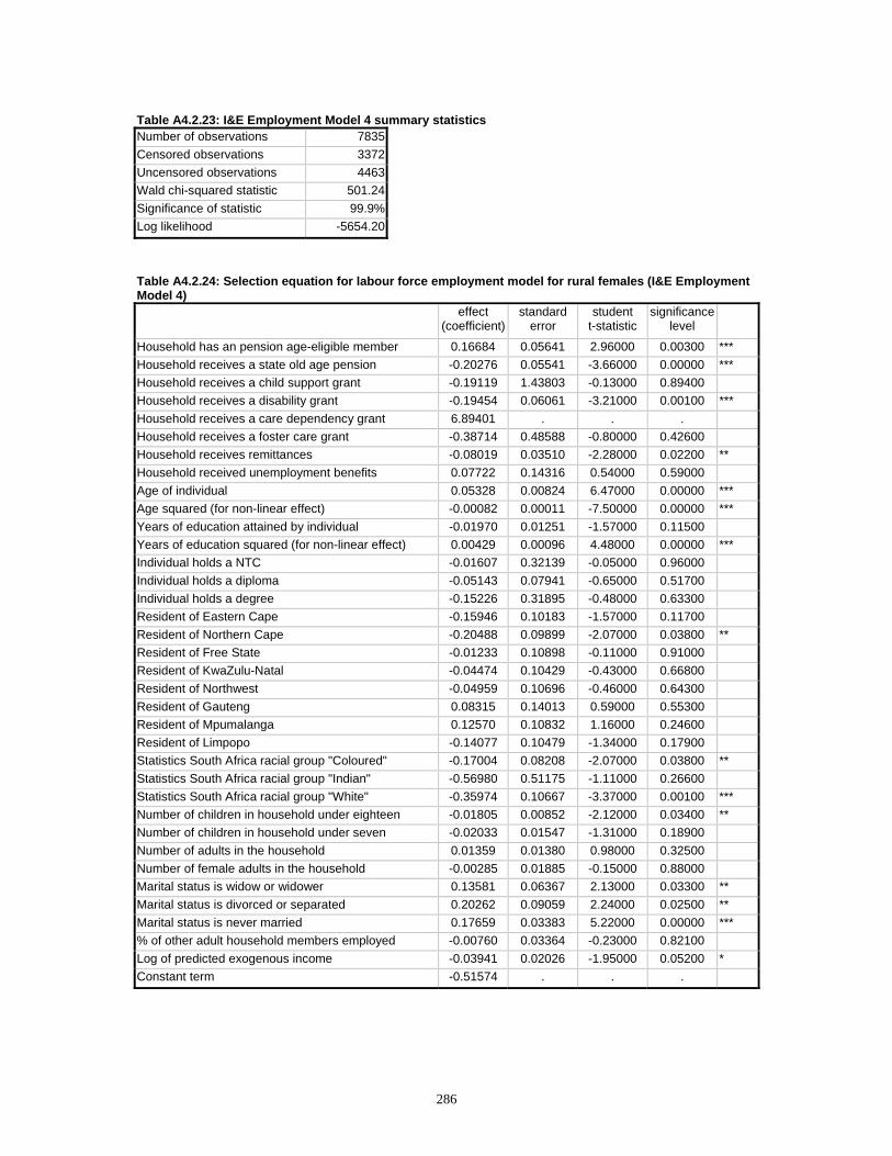
286
Table A4.2.23: I&E Employment Model 4 summary statistics Number of observations 7835Censored observations 3372Uncensored observations 4463Wald chi-squared statistic 501.24Significance of statistic 99.9%Log likelihood -5654.20
Table A4.2.24: Selection equation for labour force employment model for rural females (I&E Employment Model 4)
effect (coefficient)
standard error
student t-statistic
significance level
Household has an pension age-eligible member 0.16684 0.05641 2.96000 0.00300 *** Household receives a state old age pension -0.20276 0.05541 -3.66000 0.00000 *** Household receives a child support grant -0.19119 1.43803 -0.13000 0.89400 Household receives a disability grant -0.19454 0.06061 -3.21000 0.00100 *** Household receives a care dependency grant 6.89401 . . . Household receives a foster care grant -0.38714 0.48588 -0.80000 0.42600 Household receives remittances -0.08019 0.03510 -2.28000 0.02200 ** Household received unemployment benefits 0.07722 0.14316 0.54000 0.59000 Age of individual 0.05328 0.00824 6.47000 0.00000 *** Age squared (for non-linear effect) -0.00082 0.00011 -7.50000 0.00000 *** Years of education attained by individual -0.01970 0.01251 -1.57000 0.11500 Years of education squared (for non-linear effect) 0.00429 0.00096 4.48000 0.00000 *** Individual holds a NTC -0.01607 0.32139 -0.05000 0.96000 Individual holds a diploma -0.05143 0.07941 -0.65000 0.51700 Individual holds a degree -0.15226 0.31895 -0.48000 0.63300 Resident of Eastern Cape -0.15946 0.10183 -1.57000 0.11700 Resident of Northern Cape -0.20488 0.09899 -2.07000 0.03800 ** Resident of Free State -0.01233 0.10898 -0.11000 0.91000 Resident of KwaZulu-Natal -0.04474 0.10429 -0.43000 0.66800 Resident of Northwest -0.04959 0.10696 -0.46000 0.64300 Resident of Gauteng 0.08315 0.14013 0.59000 0.55300 Resident of Mpumalanga 0.12570 0.10832 1.16000 0.24600 Resident of Limpopo -0.14077 0.10479 -1.34000 0.17900 Statistics South Africa racial group "Coloured" -0.17004 0.08208 -2.07000 0.03800 ** Statistics South Africa racial group "Indian" -0.56980 0.51175 -1.11000 0.26600 Statistics South Africa racial group "White" -0.35974 0.10667 -3.37000 0.00100 *** Number of children in household under eighteen -0.01805 0.00852 -2.12000 0.03400 ** Number of children in household under seven -0.02033 0.01547 -1.31000 0.18900 Number of adults in the household 0.01359 0.01380 0.98000 0.32500 Number of female adults in the household -0.00285 0.01885 -0.15000 0.88000 Marital status is widow or widower 0.13581 0.06367 2.13000 0.03300 ** Marital status is divorced or separated 0.20262 0.09059 2.24000 0.02500 ** Marital status is never married 0.17659 0.03383 5.22000 0.00000 *** % of other adult household members employed -0.00760 0.03364 -0.23000 0.82100 Log of predicted exogenous income -0.03941 0.02026 -1.95000 0.05200 * Constant term -0.51574 . . .
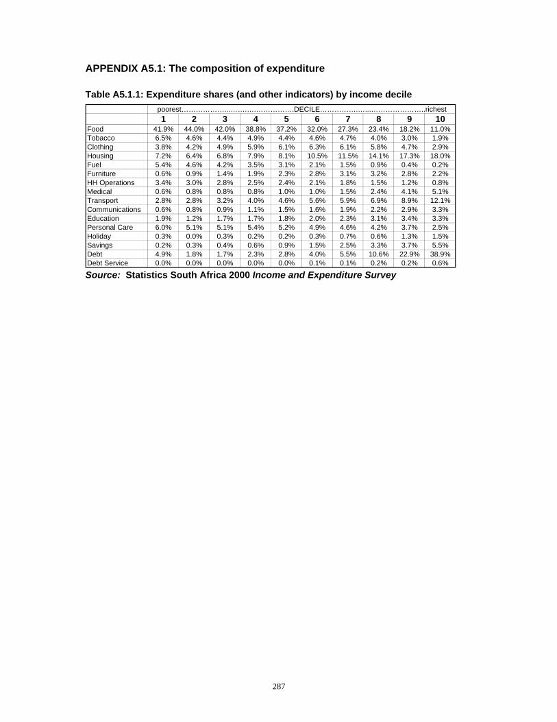
287
APPENDIX A5.1: The composition of expenditure Table A5.1.1: Expenditure shares (and other indicators) by income decile
Source: Statistics South Africa 2000 Income and Expenditure Survey
1 2 3 4 5 6 7 8 9 10Food 41.9% 44.0% 42.0% 38.8% 37.2% 32.0% 27.3% 23.4% 18.2% 11.0%Tobacco 6.5% 4.6% 4.4% 4.9% 4.4% 4.6% 4.7% 4.0% 3.0% 1.9%Clothing 3.8% 4.2% 4.9% 5.9% 6.1% 6.3% 6.1% 5.8% 4.7% 2.9%Housing 7.2% 6.4% 6.8% 7.9% 8.1% 10.5% 11.5% 14.1% 17.3% 18.0%Fuel 5.4% 4.6% 4.2% 3.5% 3.1% 2.1% 1.5% 0.9% 0.4% 0.2%Furniture 0.6% 0.9% 1.4% 1.9% 2.3% 2.8% 3.1% 3.2% 2.8% 2.2%HH Operations 3.4% 3.0% 2.8% 2.5% 2.4% 2.1% 1.8% 1.5% 1.2% 0.8%Medical 0.6% 0.8% 0.8% 0.8% 1.0% 1.0% 1.5% 2.4% 4.1% 5.1%Transport 2.8% 2.8% 3.2% 4.0% 4.6% 5.6% 5.9% 6.9% 8.9% 12.1%Communications 0.6% 0.8% 0.9% 1.1% 1.5% 1.6% 1.9% 2.2% 2.9% 3.3%Education 1.9% 1.2% 1.7% 1.7% 1.8% 2.0% 2.3% 3.1% 3.4% 3.3%Personal Care 6.0% 5.1% 5.1% 5.4% 5.2% 4.9% 4.6% 4.2% 3.7% 2.5%Holiday 0.3% 0.0% 0.3% 0.2% 0.2% 0.3% 0.7% 0.6% 1.3% 1.5%Savings 0.2% 0.3% 0.4% 0.6% 0.9% 1.5% 2.5% 3.3% 3.7% 5.5%Debt 4.9% 1.8% 1.7% 2.3% 2.8% 4.0% 5.5% 10.6% 22.9% 38.9%Debt Service 0.0% 0.0% 0.0% 0.0% 0.0% 0.1% 0.1% 0.2% 0.2% 0.6%
poorest………………...…….….…………….DECILE…………….…...…………………..richest
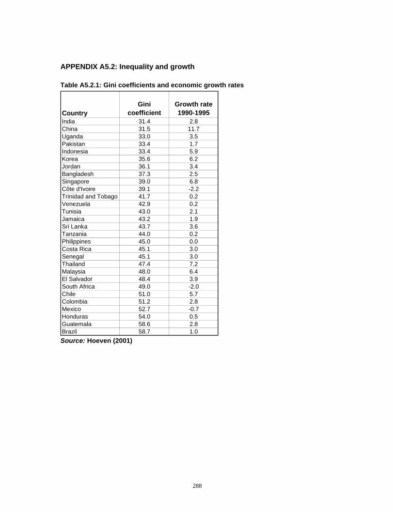
288
APPENDIX A5.2: Inequality and growth Table A5.2.1: Gini coefficients and economic growth rates
Source: Hoeven (2001)
CountryGini
coefficientGrowth rate 1990-1995
India 31.4 2.8China 31.5 11.7Uganda 33.0 3.5Pakistan 33.4 1.7Indonesia 33.4 5.9Korea 35.6 6.2Jordan 36.1 3.4Bangladesh 37.3 2.5Singapore 39.0 6.8Côte d'Ivoire 39.1 -2.2Trinidad and Tobago 41.7 0.2Venezuela 42.9 0.2Tunisia 43.0 2.1Jamaica 43.2 1.9Sri Lanka 43.7 3.6Tanzania 44.0 0.2Philippines 45.0 0.0Costa Rica 45.1 3.0Senegal 45.1 3.0Thailand 47.4 7.2Malaysia 48.0 6.4El Salvador 48.4 3.9South Africa 49.0 -2.0Chile 51.0 5.7Colombia 51.2 2.8Mexico 52.7 -0.7Honduras 54.0 0.5Guatemala 58.6 2.8Brazil 58.7 1.0
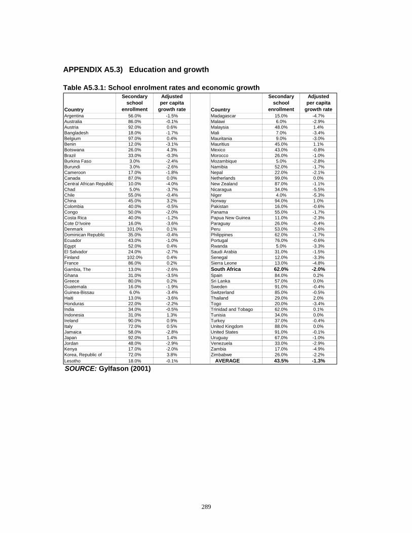
289
APPENDIX A5.3) Education and growth Table A5.3.1: School enrolment rates and economic growth
SOURCE: Gylfason (2001)
Country
Secondary school
enrollment
Adjusted per capita
growth rate Country
Secondary school
enrollment
Adjusted per capita
growth rateArgentina 56.0% -1.5% Madagascar 15.0% -4.7%Australia 86.0% -0.1% Malawi 6.0% -2.9%Austria 92.0% 0.6% Malaysia 48.0% 1.4%Bangladesh 18.0% -1.7% Mali 7.0% -3.4%Belgium 97.0% 0.4% Mauritania 9.0% -3.0%Benin 12.0% -3.1% Mauritius 45.0% 1.1%Botswana 26.0% 4.3% Mexico 43.0% -0.8%Brazil 33.0% -0.3% Morocco 26.0% -1.0%Burkina Faso 3.0% -2.4% Mozambique 5.0% -2.8%Burundi 3.0% -2.6% Namibia 52.0% -1.7%Cameroon 17.0% -1.8% Nepal 22.0% -2.1%Canada 87.0% 0.0% Netherlands 99.0% 0.0%Central African Republic 10.0% -4.0% New Zealand 87.0% -1.1%Chad 5.0% -3.7% Nicaragua 34.0% -5.5%Chile 55.0% -0.4% Niger 4.0% -5.3%China 45.0% 3.2% Norway 94.0% 1.0%Colombia 40.0% -0.5% Pakistan 16.0% -0.6%Congo 50.0% -2.0% Panama 55.0% -1.7%Costa Rica 40.0% -1.2% Papua New Guinea 11.0% -2.3%Cote D’Ivoire 16.0% -3.6% Paraguay 26.0% -0.4%Denmark 101.0% 0.1% Peru 53.0% -2.6%Dominican Republic 35.0% -0.4% Philippines 62.0% -1.7%Ecuador 43.0% -1.0% Portugal 76.0% -0.6%Egypt 52.0% 0.4% Rwanda 5.0% -3.3%El Salvador 24.0% -2.7% Saudi Arabia 31.0% -1.5%Finland 102.0% 0.4% Senegal 12.0% -3.3%France 86.0% 0.2% Sierra Leone 13.0% -4.8%Gambia, The 13.0% -2.6% South Africa 62.0% -2.0%Ghana 31.0% -3.5% Spain 84.0% 0.2%Greece 80.0% 0.2% Sri Lanka 57.0% 0.0%Guatemala 16.0% -1.9% Sweden 91.0% -0.4%Guinea-Bissau 6.0% -3.4% Switzerland 85.0% -0.5%Haiti 13.0% -3.6% Thailand 29.0% 2.0%Honduras 22.0% -2.2% Togo 20.0% -3.4%India 34.0% -0.5% Trinidad and Tobago 62.0% 0.1%Indonesia 31.0% 1.3% Tunisia 34.0% 0.0%Ireland 90.0% 0.9% Turkey 37.0% -0.4%Italy 72.0% 0.5% United Kingdom 88.0% 0.0%Jamaica 58.0% -2.8% United States 91.0% -0.1%Japan 92.0% 1.4% Uruguay 67.0% -1.0%Jordan 48.0% -2.9% Venezuela 33.0% -2.9%Kenya 17.0% -2.0% Zambia 17.0% -4.9%Korea, Republic of 72.0% 3.8% Zimbabwe 26.0% -2.2%Lesotho 18.0% -0.1% AVERAGE 43.5% -1.3%