THE SLEUTH URBAN GROWTH MODEL AS FORECASTING

AND DECISION-MAKING TOOL BRENDON MILES WATKISS Thesis presented in partial fulfilment of the requirements for the degree of

Master of Natural Sciences at the University of Stellenbosch

Supervisor: Prof. JH. Van der Merwe March 2008

ii

Declaration

I, the undersigned, hereby declare that the work contained in this thesis is my own original work

and that I have not previously in its entirety or in part submitted it at any university for a degree

Signature: ____ ____

Copyright ©2007 Stellenbosch University

All rights reserved

iii

ABSTRACT

Accelerating urban growth places increasing pressure not only on the efficiency of infrastructure

and service provision, but also on the natural environment. City managers are delegated the task of

identifying problem areas that arise from this phenomenon and planning the strategies with which to

alleviate them. It is with this in mind that the research investigates the implementation of an urban

growth model, SLEUTH, as a support tool in the planning and decision making process. These

investigations are carried out on historical urban data for the region falling under the control of the

Cape Metropolitan Authority. The primary aim of the research was to simulate future urban

expansion of Cape Town based on past growth patterns by making use of cellular automata

methodology in the SLEUTH modeling platform.

The following objectives were explored, namely to: a) determine the impact of urbanization on the

study area, b) identify strategies for managing urban growth from literature, c) apply cellular

automata as a modeling tool and decision-making aid, d) formulate an urban growth policy based on

strategies from literature, and e) justify SLEUTH as the desired modeling framework from

literature. An extensive data base for the study area was acquired from the product of a joint

initiative between the private and public sector, called “Urban Monitoring”. The data base included:

a) five historical urban extent images (1977, 1988, 1993, 1996 and 1998); b) an official urban buffer

zone or ‘urban edge’, c) a Metropolitan Open Space System (MOSS) database, d) two road

networks, and d) a Digital Elevation Model (DEM). Each dataset was converted to raster format in

ArcEdit and finally .gif images were created of each data layer for compliance with SLEUTH

requirements. SLEUTH processed this historic data to calibrate the growth variables for best fit of

observed historic growth. An urban growth forecast was run based on the calibration parameters.

Findings suggest SLEUTH can be applied successfully and produce realistic projection of urban

expansion. A comparison between modelled and real urban area revealed 76% model accuracy. The

research then attempts to mimic urban growth policy in the modeling environment, with mixed

results.

iv

OPSOMMING

Versnelde stedelike groei plaas verhoogde druk op, nie net die effektiwiteit van infrastruktuur- en

dienste-voorsiening nie, maar ook op die natuurlike omgewing. Stadsbestuurders het die taak om

probleemareas wat voortspruit uit hierdie verskynsel te identifiseer en om verligtingstrategieë te

beplan. Daarmee in gedagte, ondersoek die navorsing die implementering van ’n stedelike

ontwikkelingsmodel, SLEUTH, as steuninstrument vir die beplannings- en besluitnemingsproses.

Hierdie ondersoek is uitgevoer op historiese stedelike data vir die streek onder die beheer van die

Kaapse Metropool. Die primêre doel van die navorsing was om toekomstige stedelike uitbreiding

van Kaapstad te simuleer, gebaseer op historiese ontwikkelingspatrone en die gebruik van die

sellulêre outomaat-metodiek in die SLEUTH modelleringsprogram.

Die volgende doelwitte is gestel: a) bepaal die impak van verstedeliking op die studiegebied; b)

identifiseer strategieë vir die bestuur van stedelike ontwikkeling; c) pas sellulêre outomata toe as

modelleringsmeganisme vir besluitsteun; d) formuleer ’n stedelike ontwikkelingsbeleid gebaseer op

strategieë uit die literatuur; e) evalueer SLEUTH as ’n modelleringsraamwerk uit die literatuur. ’n

Omvattende databasis vir die studiegebied is onttrek uit die “Urban Monitoring” inisiatief − ’n

gesamentlike poging tussen die private en openbare sektore. Die databasis het ingesluit: a) vyf

historiese stedelike uitbreidingsbeelde (1977, 1988, 1993, 1996 en 1998); b) ’n amptelike stedelike

buffersone of stadsrand; c) ’n Metropolitaanse Oop Spasie Stelsel (MOSS); d) twee padnetwerke,

en e) ’n Digitale Elevasiemodel (DEM). Elke datastel is in ArcEdit omgeskakel na raster-formaat

en afgevoer as -beelde in .gif-formaat om aan SLEUTH se vereistes te voldoen. Hierdie historiese

data is deur SLEUTH geprosesseer om die ontwikkelingsveranderlikes te kalibreer om

waargeneemde historiese ontwikkelingspatrone ten beste te pas. Stedelike uitbreiding is daarna

voorspel volgens hierdie parameters. Die bevindings dui daarop dat SLEUTH suksesvol toegepas

kan word om realistiese projeksies van stedelike uitbreiding te maak. ’n Vergelyking tussen

gemodelleerde en ware stedelike gebiede toon ’n 76% vlak van akkuraatheid. Die poging om die

effek van stedelike ontwikkelingsbeleid met modellering na te boots, lewer gemengde resultate.

v

Acknowledgements

I thank my family for their emotional, spiritual and financial support for all my years of study.

Thank you for the doors you’ve opened and the blessing you are in my life.

To Sherry, my beautiful fiancé, whom I love very much. Thank you for all your love. For the hours

you’ve invested and for your patience.

Thanks be to God for all these people and for leading me down this road.

vi

CONTENTS

ABSTRACT iii OPSOMMING iv Acknowledgements v CHAPTER 1: URBAN GROWTH AS A RESEARCH PROBLEM 1

1.1 REAL-WORLD PROBLEM TRENDS IN URBAN EXPANSION 1

1.2 FINDING TECHNICAL PLANNING SOLUTIONS 1

1.3 RESEARCH PROBLEM 2

1.4 RESEARCH AIM AND OBJECTIVES 3

1.4.1 Research aim 3

1.4.2 Research objectives 3

1.5 DEMARCATION OF THE STUDY AREA 3

1.6 RESEARCH DESIGN, DATA AND METHODOLOGY 4

1.6.1 Research Design 5

1.6.2 SLEUTH requirements and methods for data collection and analysis 5

1.7 REPORT STRUCTURE 7 CHAPTER 2: URBAN GROWTH MANAGEMENT INSTRUMENTS 8

2.1 POLICY INSTRUMENTS FOR URBAN GROWTH MANAGEMENT IN CAPE TOWN 8

2.1.1 Urbanisation and urban form in the South African context 8

2.1.2 The Metropolitan Spatial Development Framework 9

2.1.3 Related spatial management strategies 11

2.2 CELLULAR AUTOMATA AS TECHNICAL MANAGEMENT INSTRUMENT 12

2.2.1 Defining cellular automata 12

2.2.2 Data requirements of a CA model 13

2.3 THE SLEUTH MODEL AND ITS REQUIREMENTS 13

2.3.1 Model overview 14

2.3.2 SLEUTH applications examples 14

2.3.3 The urban growth dynamics simulated by SLEUTH 17

2.3.3.1 Spontaneous urban growth 18 2.3.3.2 New spreading centre urban growth 18 2.3.3.3 Urban edge-influenced growth 19 2.3.3.4 Road-influenced growth 19 2.3.3.5 Slope coefficient 20 2.3.3.6 Self-modification of growth rate allowed 21

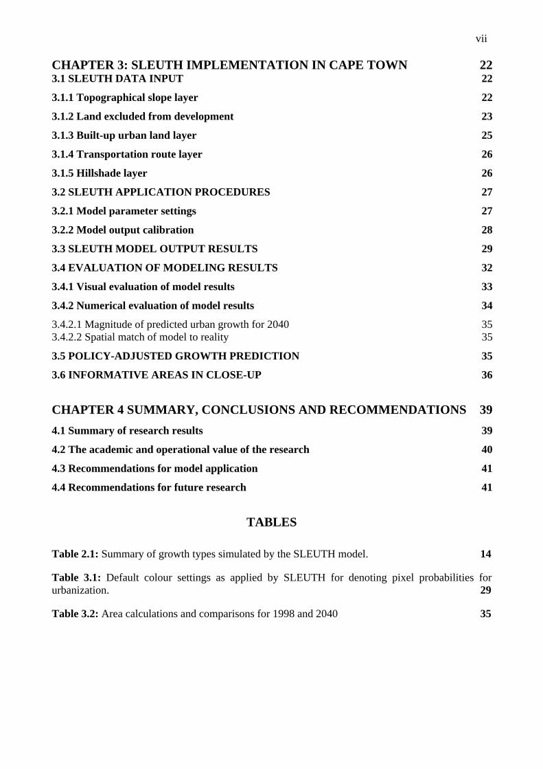
vii CHAPTER 3: SLEUTH IMPLEMENTATION IN CAPE TOWN 22 3.1 SLEUTH DATA INPUT 22

3.1.1 Topographical slope layer 22

3.1.2 Land excluded from development 23

3.1.3 Built-up urban land layer 25

3.1.4 Transportation route layer 26

3.1.5 Hillshade layer 26

3.2 SLEUTH APPLICATION PROCEDURES 27

3.2.1 Model parameter settings 27

3.2.2 Model output calibration 28

3.3 SLEUTH MODEL OUTPUT RESULTS 29

3.4 EVALUATION OF MODELING RESULTS 32

3.4.1 Visual evaluation of model results 33

3.4.2 Numerical evaluation of model results 34

3.4.2.1 Magnitude of predicted urban growth for 2040 35 3.4.2.2 Spatial match of model to reality 35

3.5 POLICY-ADJUSTED GROWTH PREDICTION 35

3.6 INFORMATIVE AREAS IN CLOSE-UP 36

CHAPTER 4 SUMMARY, CONCLUSIONS AND RECOMMENDATIONS 39

4.1 Summary of research results 39

4.2 The academic and operational value of the research 40

4.3 Recommendations for model application 41

4.4 Recommendations for future research 41

TABLES

Table 2.1: Summary of growth types simulated by the SLEUTH model. 14

Table 3.1: Default colour settings as applied by SLEUTH for denoting pixel probabilities for urbanization. 29

Table 3.2: Area calculations and comparisons for 1998 and 2040 35

viii

FIGURES

Figure 1.1: The study area: Metropolitan Cape Town 4

Figure 1.2: Research design 5

Figure 2.1: Illustration of spontaneous urban growth 18

Figure 2.2: Illustration of new spreading centre urban growth 19

Figure 2.3: Illustration of urban edge growth 19

Figure 2.4: Illustration of road-influenced urban growth 20

Figure 2.5: Behaviour of the slope coefficient in grid modeling 20

Figure 3.1: Slope layer of the study area produced from DEM 23

Figure 3.2: Excluded from urban growth layer of the study area 24

Figure 3.3: Extent of urban development in the study area (1998 ). 25

Figure 3.4: Transportation network of the study area constituting all major transport routes for 1998. 26

Figure 3.5: Hillshade of the study area derived from DEM 27

Figure 3.6: Modeling output result: Urban extent for the seed year 1999 30

Figure 3.7: Modeling output result: Urban extent for 2010 30

Figure 3.8: Modeling output result: Urban extent for 2020 31

Figure 3.9: Modeling output result: Urban extent for 2030 31

Figure 3.10: Modeling output result: Urban extent for 2040 32

Figure 3.11: The effect of the exclusion layer and year 2040 prediction 32

Figure 3.12: Comparison of modelled and real world urban extent for 2007 34

Figure 3.13: Exaggerated growth for year 2040 36

Figure 3.14: Exaggerated growth with urban edge modification for year 2040 36

Figure 3.15: Enlarged view of a problem area under the exaggerated growth scenario 37

Figure 3.16: Enlarged view of a problem area under the urban edge modification scenario 37

REFERENCES 43

APPENDICES 45

APPENDIX A: The SLEUTH scenario file as provided with the programme download 46

ix APPENDIX B: Animation of prediction for growth coefficients derived from historic data calibration (Electronic version on CD in cover sleeve) 53

1

CHAPTER 1: URBAN GROWTH AS A RESEARCH PROBLEM

1.1 REAL-WORLD PROBLEM TRENDS IN URBAN EXPANSION

Masser (2001) states that urban growth is inevitable for the next two decades and that the majority

of this growth will occur in the developing countries. Furthermore, by 2025 at least five billion

people will be living in cities. This scenario has implications for urban planning and infrastructure

particularly within the South African context.

As a developing country, South Africa is experiencing extensive growth of its urban areas due to a

number of factors, most notably population growth via rural-urban migration and natural increase.

This urban expansion, indeed at the rapid rate in which it is occurring, “presents a formidable

challenge to urban planners and managers” (Masser 2001:503). Urban planners are faced with the

problem of upgrading heavily stressed infrastructures, while simultaneously being required to

protect the natural environment and valuable arable lands.

According to the State of Cape Town Report (City of Cape Town 2006:25) the city has increased in

area by 40% since 1985 with most of this expansion “occurring without coordinated direction,

management or alignment with infrastructure provision”. In addition, it is observed [that] “the

growth has also lacked an integrated approach to transport and land use resulting in inefficient and

costly transport systems and negative social and economic impacts.” This situation is typical of the

post-apartheid city structure in South Africa that requires new planning approaches.

1.2 FINDING TECHNICAL PLANNING SOLUTIONS

As urban planners and city managers face the challenges of urban expansion and restructuring,

access to new planning techniques and the role that technology can play in the formulation of urban

growth strategies would be beneficial, especially in predicting the influence of these strategies on

future urban extent. Dynamic spatial urban models that provide an improved ability to assess future

growth and to create planning scenarios, allowing the exploration of impacts of decisions that

follow different urban planning and management policies (Kaiser, Godschalk, & Chapin 1995;

Klostermann 1999; Herold, Goldstein & Clarke 2002) are now becoming available. The

2 combination of new spatial data and modeling methods will be able to support far better informed

decision-making for city planners, economists, urban ecologists and resource managers.

One such tool is Cellular Automata (CA), a modeling procedure which is widely suggested and

implemented by researchers of urban growth for forecasting future urban extents. According to

Silva & Clarke (2002:526), “…modeling is essential for the analysis, and especially for the

prediction, of the dynamics of urban growth.” This statement is supported by the views of Barredo,

Kasanko, McCormick & Lavalle (2003:145) who state that “the most potentially useful applications

of CA from the point of view of spatial planning, is their use in simulations of urban growth at local

and regional level.”

Li & Gar-On Yeh (2000) propose integrating CA with GIS as a tool to aid planners in the search for

better urban forms for sustainable development. Furthermore they state that “the results of modeling

can provide useful guidelines for policy making and urban management in developing countries...”

(Li & Gar-On Yeh 2000:150). At this point in time, very little evidence of research in the

application of modeling exists in the South African context.

1.3 RESEARCH PROBLEM

The lack of coordinated urban growth management together with the challenges of accelerated

urbanisation in the Cape Metropolitan region has led to a re-evaluation of management principles

and strategies to reshape the future urban footprint. There is little evidence of the incorporation of

urban growth modeling tools in the local arena, even though the subject has been widely researched

and highly praised as a decision-making tool in the global arena.

This research makes use of a Cellular Automata program known as SLEUTH, which was created by

Professor Keith Clarke (Candau, Rasmussen & Clarke 2000) and is currently used by the United

States Geological Survey (USGS s.d.) in “Project Gigalopolis”, aimed at investigating urban growth

in the United States. The question arises: Can SLEUTH be used in a South African context to

usefully project, manage and monitor ‘natural’ urban growth and the effect of urban expansion

policies in the South African setting offered by Cape Town?

3

1.4 RESEARCH AIM AND OBJECTIVES

To guide and direct the research process and the application of the chosen methodology, a clear

research aim and set of research objectives have been formulated at the outset.

1.4.1 Research aim

The thesis aims to simulate future urban expansion of Cape Town, by making use of cellular

automata methodology in the SLEUTH modeling platform from empirically mapped past urban

growth extent patterns over an extended period, and to show the effect of policy measures to contain

the unfolding growth pattern.

1.4.2 Research objectives

To ensure that the research process remained on track throughout and was guided by the production

of concrete deliverable products, three salient research objectives were set. These objectives were

to:

- identify strategies currently formulated by the metropolitan government to manage the

extent and nature of urban growth in Cape Town;

- from literature, explore and evaluate the feasibility of cellular automata and the SLEUTH

software in particular as a modeling framework tool to simulate urban growth; and

- practically implement and evaluate the performance of the SLEUTH software to model

future urban expansion and the effect of urban policy measures in Cape Town.

The thesis subsequently reports sequentially on the conduct of these processes and the nature of the

research products through which these objectives were met.

1.5 DEMARCATION OF THE STUDY AREA

The study area is defined as the jurisdiction boundary of the Cape Metropolitan Council area and

incorporates all urban areas falling within this boundary. This area is indicated in Figure 1.1, and

4

Study AreaJurisdiction of Cape Metropolitan Council

Urban Areas within Metro Jurisdiction

Municipal Authority

stretches from Cape Point and False Bay in the south to Atlantis in the north. It includes the whole

Cape Peninsula and the Helderberg Basin containing Strand and Somerset West in the east.

Figure 1.1: The study area: Metropolitan Cape Town

This large urban region encompasses a total of some 246501ha. On the eastern and northern

periphery it is surrounded by five neighbouring municipal authorities, of which at least two

(Stellenbosch and Drakenstein-Paarl) are considered to be part of what is termed the ‘functional

region’ of Cape Town and with which extensive functional urban linkages indeed exist.

1.6 RESEARCH DESIGN, DATA AND METHODOLOGY

Attaining the objectives required a particular research design to be followed and specific spatially

formatted data to be gathered according to acceptable scientific standards. This section in the

various rubrics provides the necessary detail to judge the scientific standard of the work by.

5

1.6.1 Research Design

As Figure 1.2 indicates, the research was conducted according to a series of succinct analytical

steps.

Figure 1.2: Research design

Firstly, the spatial extent of urban land coverage had to be obtained for five time intervals spanning

a 20-year period in map form and then converted into a format suitable for SLEUTH application.

The model had to be calibrated by using the trends in these spatial images before the simulation of

future patterns could be generated. Finally the possible effect of urban management policies could

be mimicked and the modelled results compared with the real-world patterns observed, to be able to

evaluate the efficacy of the SLEUTH model.

1.6.2 SLEUTH requirements and methods for data collection and analysis

The SLEUTH Urban Growth Model is an open source package and is available to the public on the

USGS affiliated, Project Gigalopolis (USGS s.d.), at its research webpage

www.ncgia.ucsb.edu/projects/gig/. Several versions of SLEUTH as well as its forerunner; the Urban

Data analysis and conversion to SLEUTH data input

requirements

Calibrate model using historical data.

1977

1988

1993

1996

1998

Produce simulation of growth from 1998 to 2040.

Compare modeled 2007 output extent to real world 2007 extent derived from a shapefile database of all surveyed land parcels extracted for the study area, acquired from the Offices of the Surveyor General (Cape Town).

Manipulate variables to mimic possible policy scenarios.

6 Growth Model are available. The earliest versions of SLEUTH are ported for platforms running the

UNIX operating system, however the latest SLEUTH release (June 2005) is ported for both UNIX

and Linux compatibility. The version of SLEUTH used in this investigation is a UNIX release

modified by Professor Larry Zietsman of Stellenbosch University for operation on the Microsoft

DOS platform.

SLEUTH is an acronym derived from the input data requirements of the urban growth model: Slope,

Land-use, Excluded, Urban, Topology, Hillshade. The model requires the compilation of a data

base comprising a broad spectrum of data types. These data must be standardized and reformatted to

SLEUTH requirements. The data set applied in this research was primarily the product of a joint

initiative between the public and private sector named “Urban Monitoring” the chief role-player of

which being The City of Cape Towns Department of Strategy and Planning, Spatial Planning and

Urban Design. The project sought to gain an understanding of the growth patterns shaping the City

of Cape Town by comparing graphic representations of the City’s spatial extent for several time

periods. The data comprised of five historic data layers of urban extent for the years 1977, 1988,

1993, 1996 and 1998 compiled and digitally stored in shapefile format. The years identified for

inclusion in the database were dictated by the availability of historic aerial photography. The aerial

photography used in the project was 1:10000 orthographic imagery. Methodology for data capture

required the imagery to be scanned and geographically corrected within a digital database. The

images were then viewed in the ESRI ArcGIS software environment, and urban areas were

identified manually and digitized on screen. To improve the accuracy of identification in the more

recent years (1996; 1998), a shapefile database of all surveyed land parcels (erven) for the

corresponding years was overlaid upon the imagery to assist in the identification of smaller

developed erven (< = 5000m²). Apart from historic urban extent data gathered for SLEUTH input, a

database of surveyed erven for 2007 was also acquired from the Office of the Surveyor General to

aid in the evaluation of SLEUTH modeling output. Processing of this data layer is discussed in

section 3.4.

Furthermore, a Metropolitan Open Space System (MOSS) database was included to facilitate the

production of a layer showing areas that would be excluded from all development. The MOSS

database represents areas identified as having conservation, agricultural, recreational or cultural

value for preservation both within the City, and areas beyond the urban footprint, earmarked for

protection in the future. Two major road networks incorporating major links such as freeways, main

roads, national routes and arterial roads representative of 1988 and 1998, were extracted from a road

database digitized from 1:50 000 topographical maps, produced and maintained by the Chief

7 Directorate of Surveys and Mapping. Finally, a Digital Elevation Model (DEM) of 20m resolution

was produced by creating a Triangular Irregular Network (TIN) from a 20m contour line shapefile

database produced and maintained by the Chief Directorate of Surveys and Mapping. This TIN was

converted to a DEM using ESRI ArcGIS functionality, from which the Hillshade, Slope, and

Topology layers were subsequently produced using further ESRI ArcGIS functionality. The land-

use modeling functionality of the model was not required for the purposes of the study, thus no

land-use data was acquired.

The acquired spatial data were clipped to a common extent and converted to a common projection.

All Arc shape files were converted to raster grids by using the PolyGrid command in ArcEdit. All

rasterized data were then resampled to a common pixel resolution and converted to greyscale .tiff

image format with the ArcEdit command, Gridimage. Finally, the .tiff images were converted to

SLEUTH compatible .gif image format using the Photoshop photo editor. The actual application of

SLEUTH is reported on in the relevant content section.

1.7 REPORT STRUCTURE

The report in Chapter 1 introduces the phenomenon of urbanization, the problems that are

associated with it in the realms of urban management and planning, and a modeling tool to aid

decision makers in this area is briefly described together with the data particulars for the research.

Chapter 2 expands the topic of urbanization in the South African context and highlights

management strategies identified for managing the problems arising. Also included there, is an

exploration in greater depth, of the SLEUTH urban growth model. Chapter 3 provides an overview

of the data applied in the model, from which growth statistics are derived through a calibration

process. The output of model prediction is presented in this same chapter in which the model is

further explored for accuracy and scenario modeling capability. In Chapter 4 a summary of results

and conclusions are drawn from the various observations and recommendations for application and

further research are presented.

8

CHAPTER 2: URBAN GROWTH MANAGEMENT INSTRUMENTS

Local authorities endeavour to deal with and manage urban growth in a variety of ways. The

argument here will be that such management may take the form of policy/government instruments

to guide growth trends and also to aid this process and monitor its progress or viability by recourse

to technological instruments by which the spatially manifested effects of policy implementation

may be simulated. Therefore this chapter is divided into two sections; firstly an overview of urban

policy instruments devised for spatial governance in Cape Town, followed by an exposé of Cellular

Automata and particularly the SLEUTH software modeling platform by which the effects of these

policies may be technically simulated.

2.1 POLICY INSTRUMENTS FOR URBAN GROWTH MANAGEMENT IN CAPE TOWN

Cape Town suffers from typical South African spatio-morphological problems and hence this

background needs initial discussion in this section. Then follow sections on the MSDF and related

policy instruments specifically designed by city authorities to address its unique spatial

development trends.

2.1.1 Urbanisation and urban form in the South African context

The unique history of South Africa is reflected in the structure of its cities. At their inception towns

inherited the structure of their colonial counterparts, the grid pattern, established on the European

continent (Davies, 1963). As populations increased, so too the disorder and public health issues,

which at the turn of the century led to an urban management approach which sought to curtail urban

growth by controlling city life. The rise of apartheid saw these laws expanded and rigorously

enforced, to the point of completely reshaping the urban landscape and minimizing expansion by

controlling movement in and out of urban areas of certain population groups.

Three distinct spatial patterns are evident in South African cities and continue to influence urban

form; the first of these is low density urban sprawl, attributed to local government’s efforts to both

accommodate the expansion of affluent households into peri-urban areas and to contain the growth

of informal settlements beyond the urban edge. Secondly, zoning legislation and land and housing

policies, formulated to reduce contact between racial groups, led to fragmentation as development

9 occurred in discrete pockets separated by physical boundaries such as freeways and open spaces.

Thirdly, an urban management philosophy which separated land uses, race and income groups,

attributed to the separation of places of work and residence. These urban management practices led

to the rapid growth of townships on the urban fringe as these accommodated both the urban poor

and segregated population as well as rural migrants seeking better opportunities and living

conditions from the rural areas (Smith, s.d.)

In the case of Cape Town, the massive growth of townships has accounted for approximately 80%

of recent population growth. Consider the following statistics according to the State of Cape Town

Report (City of Cape Town 2006): the urban footprint grew by 40% in the period 1985 to 2005;

from 1977 to 1988 the city was expanding in developed area by an average of 701 hectares per year;

by 2006 this figure was nearly double at 1232 hectares per year. As the city expands in area, so too

do the challenges that face urban planners. Large quantities of natural resources are expended each

year, infrastructure must be expanded and the natural habitat and economic farming sectors must be

protected. Urban sprawl which is attributed to accelerated growth in low-density suburban

residential developments, contributes to increased commuting times and congestion, the loss of

valuable agricultural land and areas of high biodiversity value, and increased cost of providing

services such as piped water, sewers, drains and roads.

The State of Cape Town Report of 2006 states clearly that “[the] current urban form is

unsustainable, economically unproductive and prevents spatial, racial and economic integration.”

(City of Cape Town 2006:25). It is with these challenges in mind that town managers and planners

formulate guidelines to direct future expansion and serve as a point of departure for the

establishment of policies to curb urban sprawl and to enforce the adherence to developmental

regulations.

2.1.2 The Metropolitan Spatial Development Framework

The Metropolitan Spatial Development Framework (MSDF) outlines the vision for the future

spatial form of Cape Town and provides the necessary guidelines to realize the vision for future

expansion. This document, released in 1996, has since been revised and expanded, yet the core

objectives remain central to the management initiative. The MSDF was endorsed by the Cape

Metropolitan Council (CMC) in April 1996 and is available as a Technical Report (Metropolitaanse

Ruimtelike Ontwikkelingsraamwerk 1996). Its primary function is to serve as a guide for spatial

10 development in the Cape Metropolitan functional region. Much of what follows summarise and

capture salient policy aspects from this document.

The core purpose of the MSDF was to guide the form and location of physical development in the

Cape Metropolitan Region (CMR) on a metropolitan scale.

It highlighted four areas of focus, namely:

- providing direction for physical growth at metropolitan scale;

- providing spatial direction to Reconstruction and Development projects (RDP);

- providing a framework for co-ordinated action between the public, private and

community sectors; and

- providing the basis for the preparation of policies, programmes and development

strategies at local and metropolitan levels.

Furthermore the document proceeded to outline both the spatial and non-spatial guidelines required

to meet these goals. The spatial guidelines are specifically aimed at:

- management of all urban resources to ensure sustainability in utilization;

- containing urban sprawl;

- intensifying urban development within the existing urban areas;

- integrating isolated urban area through mixed-use development, public transport and road

network connectivity;

- redressing imbalances in the location of urban services and employment opportunities;

and

- developing quality urban environments.

The non-spatial guidelines include aims for:

- ensuring that development is people-driven;

- co-ordinating spatial planning with economic and social development policy;

- focusing public investment on identified priority areas; and

- planning and goal-setting linked to budgeting and financing.

The MSDF therefore clearly provides a broad framework within which further policies could then

be formulated to achieve specific urban development outcomes.

11

2.1.3 Related spatial management strategies

As the MSDF’s functional approach, four spatial strategies were identified through which these

guidelines could be implemented: Metropolitan Urban Nodes, Metropolitan Activity Corridors, A

Metropolitan Open Space System (MOSS), and the Urban Edge. Although the MSDF failed in its

endeavour “because it assumed that it could redirect economic trends” (City of Cape Town 2006) it

did highlight areas of concern and provided a foundation upon which future planning initiatives

could be expanded and improved.

Recently the State of Cape Town Report (City of Cape Town 2006) presented an extensive proposal

and growth options for the “Planning for Future Cape Town” initiative; a long-term development

path and planning logic for the spatial form and structure of a future Cape Town which may take 40

to 100 years to realise. Five strategic areas of action are recognised (City of Cape Town 2006):

- Protecting natural assets and developing a quality open space system;

- Redefining and developing a new economic backbone for the city;

- Developing an equitable pattern of access;

- Developing an integrated city development path; and

- Developing a new pattern of special places

For each of these goals to be realized, the city’s growth must be contained and directed.

Development, therefore, should occur within the urban footprint and promote densification of units.

Vacant land within the urban footprint must be prioritised for development and infrastructure in

older areas must be upgraded. Furthermore, high potential agricultural land is to be protected, thus

any expansion threatening these areas needs to be deflected. Investment in integrated growth nodes

and integrated transport and land use is needed, and the public transport system must be expanded

and improved to serve both business and the community.

While these plans provide direction and guidance on paper, it is difficult to envisage how they could

influence the city in the space of five years, much less twenty. Ideally the more information

available to planners the more confident they can be in their decision making processes. Previous

attempts have been made to use computerised stochastic simulation of urban expansion, particularly

in the case of Cape Town (Van der Merwe 1980), but more recent spatial information technology

and a modeling process known as Cellular Automata may provide an even better solution. It has

been explored in the realms of urban modeling, where Li & Gar-On Yeh (2000:131) maintain that

12 geographers can apply “CA to simulate land use change, urban development and other changes of

geographical phenomena.”

2.2 CELLULAR AUTOMATA AS TECHNICAL MANAGEMENT INSTRUMENT

In order to gain a better understanding of Cellular Automata (CA), the research discusses its

application and operation in this section, before applying it in the next chapter. Possible

shortcomings will be explored as well as the possibility of successfully implementing CA as a

decision-making tool. One such model, the SLEUTH Urban Growth Model, is explored in great

detail.

2.2.1 Defining cellular automata

Batty (1997:266) defines CA as “…models in which contiguous or adjacent cells, such as those that

might comprise a rectangular grid, change their states − their attributes or characteristics − through

the repetitive application of simple rules.” According to Li & Gar-On Yeh (2000:131) “[a] CA

system usually consists of four elements − cells, states, neighbourhoods and rules.” These authors

continue to explain that the spatial cell is the smallest unit of the model, and that each cell has an

adjacency or proximity value. A cell’s state can be changed by transition rules that are defined by

neighbourhood functions.

Torrens & O’Sullivan (2001) define a CA as a lattice of cells, where each cell can exist in any

number of finite allowed states that will change depending on the states of its neighbouring cells,

which are influenced by a uniformly applied set of transition rules. In addition, they too mention the

four elements sited by Li & Gar-On Yeh (2000); however, they do add a fifth element, namely the

temporal component. Furthermore Torrens & O’Sullivan (2001) examine how CA can be

manipulated and programmed toward specific objectives and approaches depending on the

requirements of their application.

Clarke (s.d.), who is at the forefront of CA model development, first introduced a model labelled

the Clarke Urban Growth Model (UGM). This early model merely perpetuated transitions between

two land use states, urban and non-urban. A later report by Candau, Rasmussen & Clarke (2000)

introduces a new, more robust model, SLEUTH, created by combining the UGM with a Deltatron

13 Land Use/Land Cover Model (DLM). These deltatrons are seen as ‘living’ cells that will try to

enforce change on their neighbouring cells. If no change occurs in any of their neighbouring cells

within a set period of time the cell will ‘die’. Thus a model is created in which land cover

transitions are only permanent if the new cells are supported by their neighbours. This new model

takes a turn-based approach; firstly, the UGM models the extent of land use change (urban and non-

urban), then “[t]he DLM uses CA- based rules, class transition probabilities, and local topography

to create deltatrons (bringers of change) and enforce land class transitions within homogenous land

class areas, as well as at the interface of land use/land cover types” (Candau, Rasmussen & Clarke,

2000:3).

2.2.2 Data requirements of a CA model

CA models depend on the availability of very specific spatial information sets. According to

Herold, Menz & Clarke (s.d.) the most widely used spatial datasets for the most common CA

models (such as SLEUTH) are topography and transportation infrastructure. In addition some

models require data on population density, socio-economic distribution factors, location of

employment and population distribution and density. In short, the data requirements of the CA

model are influenced by the purpose for which the model is designed. Wilson, Hurd & Civco (2002)

states that remotely sourced data is ideally suited to CA models as it exists in raster format and is

easily classifiable into land use zones. A groundbreaking study by Compas & Sugumaran (2004)

includes the development of a web based CA model, used as a decision making tool, which makes

use almost entirely of remotely sensed data, as this data already exists to a greater degree, in digital

format. Candau (2000) states that in order for a CA to accurately model the future growth of an

urban extent, the dataset needs to include historical data of the region to be modelled, and often

requires the scanning and digitizing of historical analogue map sources. Once the required spatial

data has been gathered the process of calibrating the CA can commence.

2.3 THE SLEUTH MODEL AND ITS REQUIREMENTS

As pointed out, the SLEUTH model is at the forefront of CA development. This section reviews its

operating process, describes application examples and concludes with the simulated urban growth

dynamics processes captured by this particular instrument.

14

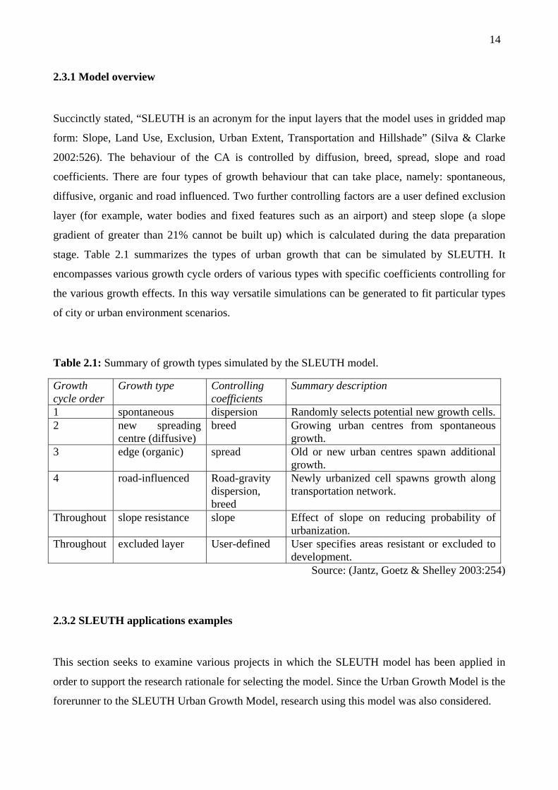
2.3.1 Model overview

Succinctly stated, “SLEUTH is an acronym for the input layers that the model uses in gridded map

form: Slope, Land Use, Exclusion, Urban Extent, Transportation and Hillshade” (Silva & Clarke

2002:526). The behaviour of the CA is controlled by diffusion, breed, spread, slope and road

coefficients. There are four types of growth behaviour that can take place, namely: spontaneous,

diffusive, organic and road influenced. Two further controlling factors are a user defined exclusion

layer (for example, water bodies and fixed features such as an airport) and steep slope (a slope

gradient of greater than 21% cannot be built up) which is calculated during the data preparation

stage. Table 2.1 summarizes the types of urban growth that can be simulated by SLEUTH. It

encompasses various growth cycle orders of various types with specific coefficients controlling for

the various growth effects. In this way versatile simulations can be generated to fit particular types

of city or urban environment scenarios.

Table 2.1: Summary of growth types simulated by the SLEUTH model.

Growth cycle order

Growth type Controlling coefficients

Summary description

1 spontaneous dispersion Randomly selects potential new growth cells.2 new spreading

centre (diffusive) breed Growing urban centres from spontaneous

growth. 3 edge (organic) spread Old or new urban centres spawn additional

growth. 4 road-influenced Road-gravity

dispersion, breed

Newly urbanized cell spawns growth along transportation network.

Throughout slope resistance slope Effect of slope on reducing probability of urbanization.

Throughout excluded layer User-defined User specifies areas resistant or excluded to development.

Source: (Jantz, Goetz & Shelley 2003:254)

2.3.2 SLEUTH applications examples

This section seeks to examine various projects in which the SLEUTH model has been applied in

order to support the research rationale for selecting the model. Since the Urban Growth Model is the

forerunner to the SLEUTH Urban Growth Model, research using this model was also considered.

15 In their article, Clarke & Gaydos (1998) combine a CA and Geographical Information Systems

(GIS) to produce a long-term urban growth prediction for the San Francisco and

Washington/Baltimore urban areas. The model used is the Urban Growth Model (UGM) developed

by Clarke. The project seeks to test the ability of the model to predict growth in areas with distinctly

different growth trends. Historical data for the two regions is used to calibrate the model, after

which the process of forecasting commences. The role played by GIS is also explored and the

research finds that there are three main areas in which GIS plays an important role. Firstly the

system acts as a data integrator, secondly as a visualization tool to generate map displays from the

model output, and thirdly, but most importantly, the ability for a GIS to store and manipulate the

new data sets for such applications as decision making tools.

Candau, Rasmussen & Clarke (2000) introduce SLEUTH as a new model applied to an extensive

region that includes the states of Delaware, District of Columbia, Maryland, North Carolina, New

York, Pennsylvania, Virginia and West Virginia. This model is based on the original UGM,

however it is coupled with a Deltatron Land-use Model (DLM). This model uses a turn-based

approach whereby the UGM applies the standard parameters to propagate land cover change

between urban and non-urban land use for a time interval of one year. Each pixel which undergoes

change in the cycle is then tested using the deltatron parameters and will revert back to its’ original

state if these parameters are not met. Such cells are logged and an uncertainty map can be produced

if desired, this allows one to distinguish between areas of high transition confidence and areas of

transition uncertainty.

Silva & Clarke (2002) expand upon the earlier work of Clarke & Gaydos (1998) by testing the

universality of the SLEUTH model in a European context by using it to model two Portuguese

cities, Lisbon and Porto, which present very different spatial and developmental characteristics due

to topographical and ancient cultural differences. The application focuses on the calibration of the

model for the two cities, as this is the most crucial stage in ensuring a high level of modeling

accuracy. They list the purposes of the study as: “(1) to demonstrate that the same model could

apply not only to North American but also to European cities; (2) to demonstrate how important

structural and geographical differences between applications could be revealed by the calibrations

that may be of use in comparative urban study; (3) to reveal how spatial resolution improves model

performance by making the model more sensitive to local conditions; and (4) how a sequential

multistage optimization throughout different phases of calibration is the key to model application

comparison” (Silva & Clarke 2002:528). The model accurately captured the definitive growth

patterns for each city and the results were pleasing. The model is very well suited to the

16 comparative analysis of different cities, as well as providing insight as to the early growth

processes. The research does remark on the excessive amounts of CPU time required, but it was

found that the SLEUTH model is easy to use and is well suited to the environment of planning

application.

Jantz, Goetz & Shelley (2003) used the SLEUTH model to simulate the impacts of future policy

scenarios on urban land use in the Baltimore-Washington metropolitan area. The topic of concern

was the affect that urban growth is having on the water quality and health of the Chesapeake Bay

estuary and its’ tributaries. SLEUTH was used to project the extent of urban growth to the year

2030 taking into account “three different policy scenarios: (1) current trends, (2) managed growth,

and (3) ecologically sustainable growth” (Jantz, Goetz & Shelley 2003:251). SLEUTH is chosen for

the project because of its easy operation, its ability to incorporate different levels of protection for

different areas, and its easy integration with raster GIS. This view is also held by Kocabas &

Dragicevic (2004). Remotely sensed data is used as a source of historic data, with 1986 chosen as

‘seed’ year followed by 1990, 1996, and 2000. The data had to be re-scaled to a coarser scale as the

available computational resources would not have been sufficient to process a resolution finer than

45m. A Monte Carlo simulation method was applied in the calibration of the model, which required

over a week of processing time on a 16-node Beowulf PC Cluster (each node consists of an AMD

processor, a 750-MHZ CPU and 1,5-GB RAM). This is extremely time consuming and hardware

extensive, however the data set is of a large area covering 23700km2. In reviewing their results the

research found that SLEUTH produced very good output for the regional level but was not accurate

at pinpointing development at the local level. This led the research to conclude that SLEUTH is

well suited to decision making and policy analysis at the regional level; however, some refinement

is needed before the model can be applied solely for this purpose at the local level.

Yang & Lo (2003) also made use of SLEUTH in their simulation to predict urban growth and test

influences of different policy scenarios in the Atlanta metropolitan area. The focus of the project

was to determine how vegetative land cover can be affected by future urban growth and how the

natural environment can be protected. Data for the model consisted of remotely sensed satellite

imagery from 1973 to 1999. Before the model could be run the data format, resolution and

dimension had to be standardized. Due to hardware constraints the calibration process, which makes

use of Monte Carlo iterations, took roughly two weeks of CPU time. The results were encouraging,

however the researchers believe that more accurate simulations could be achieved by modifying the

model’s transition rules and considering the inclusion of more growth constraints. One concluding

remark states that the model was an effective tool “to imagine, test and choose between possible

17 future urban growth scenarios in relation to different environmental and development conditions...”

(pp485).

Goldstein, Candau & Clarke (2004) take an interesting approach to CA modeling. They apply

SLEUTH to the historic modeling of urban growth in Santa Barbara. They argue that little focus has

been placed on modeling historical urban extent as current research emphasizes the modeling of

cities of the future. The researchers maintain that “understanding the growth dynamics of a region’s

past allows more intelligent forecasts of its future” (Goldstein, Candau & Clarke 2004:125). This

form of modeling allows the researcher to explore the effects that consequences of war, economic

booms and crashes, technical innovations, and disasters had on city growth. The greatest retarding

factor to such an application is the lack of historic spatio-temporal data or the high level of

distortion in geographic data. Modeling of this kind takes far more time due to the extended period

of data acquisition, and the interpolation requirements for incomplete data sets. A modified

SLEUTH model is used to rebuild data sets by using the “past” future.

Most of the literature explored praises the power of a CA to model the urban future, and promotes

CA implementation as a decision making tool. According to Yang & Lo (2003:485) “Efforts need

to be made in order to adopt cellular modeling technology for problem solving in applied urban

studies”; however, Cheng & Masser (2004) warn that local knowledge is an important ancillary data

source for CA modeling. During the modeling process “…project planning, site selection and

temporal control needs more input from local experts...(and) local knowledge is an essential source

of qualitative information.” (Cheng & Masser 2004:193).

This review has shown conclusively that the literature strongly supports the use of SLEUTH as an

effective tool for modeling urban growth and assisting urban management functions.

2.3.3 The urban growth dynamics simulated by SLEUTH

Considerations when implementing the SLEUTH model are discussed in this section. SLEUTH

requires input data to be in raster format where each pixel is unique in its value and location in the

raster grid or lattice. Each pixel or ‘cell’s’ eligibility for ‘urbanization’ is defined firstly by an

exclusion layer, which tests whether the pixel falls within an area allocated as unsuitable for

urbanization such as a water body or user defined areas such as nature reserves, and secondly, by a

18 slope layer which is produced during the data preparation stage and records the percentage slope for

each pixels location. A pixel located on a slope greater than 21% cannot be urbanized.

Following this process the dataset is subjected to numerous simulated growth cycles, each cycle

consisting of four steps in which a specific growth dynamic is modelled:

(i) Spontaneous Growth (the effect of unforeseeable growth stimulus);

(ii) New Spreading Centres (the effect of adjacency to new urban impetus cells, typically on the

urban periphery);

(iii) Edge Growth (the effect of adjacency to existing urban cells); and

(iv) Road-Influenced Growth (the effect of adjacency to existing transportation line cells).

These dynamics concur exactly with the growth triggering mechanisms identified empirically by

Van der Merwe (1980) for Cape Town and are further explored separately below.

2.3.3.1 Spontaneous urban growth

Spontaneous growth defines the occurrence of random urbanization of land. In the cellular

automaton framework this means that any pixel may be randomly urbanized during any one of the

growth cycles. In SLEUTH this growth function is controlled by the dispersion coefficient (also

referred to as diffusion) which regulates the number of times a pixel will be randomly selected

(USGS s.d.). Figure 2.1 provides a graphic rendition of such a random switch-on process of grid

cells.

Source: (www.ncgia.ucsb.edu/projects/gig , 2005)

Figure 2.1: Illustration of spontaneous urban growth

The cells being simulated as newly ‘urbanised’ are clearly not affected by existing cell conditions.

2.3.3.2 New spreading centre urban growth

This process (or modeling step) determines whether any of the new, spontaneously urbanized cells

will become new urban spreading centres. The breed coefficient is the controlling factor during this

step and requires that a newly urbanized cell have at least two urbanized neighbouring cells before

it is recognized as a spreading centre (Project Gigalopolis at USGS s.d.). Figure 2.2 offers an

19

Source: www.ncgia.ucsb.edu, /projects/gig 2005

Figure 2.2: Illustration of new spreading centre urban growth

example of a gridded modeling instance where new growth is attracted to and encouraged by an

earlier ‘growth’ cell, leading to a clustering of new growth in its vicinity.

2.3.3.3 Urban edge-influenced growth

Edge-growth applies to both new spreading centres and existing spreading centres. The spread

coefficient identifies non-urbanized cells with at least three urbanized neighbours as having a

higher probability for urbanization (Project Gigalopolis: USGS s.d.). Figure 2.3 once more

demonstrates an example of a gridded modeling instance where new growth is attracted to and

encouraged to the edge of existing urban development (cells).

Source: www.ncgia.ucsb.edu, /projects/gig 2005

Figure 2.3: Illustration of urban edge growth

This type of development is to some extent encouraged in planning because it represents the

antithesis of so-called ‘leap-frog’ development where the existing urban edge is ‘jumped’, leading

to sprawl and sterilisation of intermediate land.

2.3.3.4 Road-influenced growth

This is the final growth step where growth is determined by both the existing transportation

infrastructure and the most recent urbanization development types covered by the previous three

steps. Once the breed coefficient has assigned a transition probability to the cells, the road gravity

coefficient is applied which seeks out the nearest road to a cell up to a maximum distance scaled

according to the proportions of the raster dataset. As Figure 2.4 shows for the usual gridded

20

Source: www.ncgia.ucsb.edu, /projects/gig 2005

Figure 2.4: Illustration of road-influenced urban growth

modeling example, if a road is found within the maximum distance of the cell, a temporary urban

cell is placed on the nearest point along that road. Next, this temporary urban cell conducts a

random walk along the road where the number of steps is determined by the dispersion coefficient.

The final location of this temporary urbanized cell is then considered as a new urban spreading

nucleus (Project Gigalopolis: USGS s.d.).

2.3.3.5 Slope coefficient

The slope coefficient influences each of the four growth types and is constant throughout the

growth cycle. In SLEUTH, cells on a slope of greater than 21% (critical slope) cannot be

urbanized. Figure 2.5 shows the terminating influence of this critical factor in allowing zero

probability for a cell being switched to ‘urban’.

Source: www.ncgia.ucsb.edu, /projects/gig 2005

Figure 2.5: Behaviour of the slope coefficient in grid modeling

As it is easier to urbanize level ground, cells in these areas will be prioritized for urbanization,

alternatively, based on the dynamic of the proportion of flat land available and the proximity of

21 established urbanized cells, urbanization on increasing slopes (but less than the critical slope) can

be accommodated (Project Gigalopolis: USGS s.d.)

2.3.3.6 Self-modification of growth rate allowed

The overall growth produced by the four growth rules explored above is referred to as the growth

rate. If the growth rate level becomes unusually high or low a second level of growth rules are

initiated. Termed self-modification rules, these rules will either increase or decrease the growth

parameters of breed, spread or dispersion. Growth rate is compared to two controlling factors in the

scenario file, namely, critical high and critical low. If the growth rate exceeds the critical high

value, the growth parameters are multiplied by a factor greater than one to simulate a growth

“boom” phase. When the critical low value is reached, the growth parameters are multiplied by a

factor less than one to simulate a lag or “bust” phase. This behaviour allows the system to simulate

the typical S-curve growth common in urban expansion (Project Gigalopolis: USGS s.d.)

22

CHAPTER 3: SLEUTH IMPLEMENTATION IN CAPE TOWN

In running SLEUTH for the Cape Town application it is necessary to firstly consider the nature and

spatial patterns displayed by the various spatial data sets prepared as input into the model. The

discussion proceeds to consider the actual implementation process and finally evaluates and

interprets the results of the application.

3.1 SLEUTH DATA INPUT

SLEUTH requires five different data layers as input for both the calibration and prediction

functions. Each layer must be compiled as a greyscale .gif image. If one wishes to model land-use,

one is able to input a sixth file, a land-use classification image. For each of these input layers, a

pixel value of zero is considered inactive or nonexistent, while all values 0<n>255 are considered

active, or existing entities for that theme. Each data image must be consistent in resolution to ensure

that pixels in all layers conform in size and location in model space. For the same reason all raw

data images gathered must conform to the same projection before processing and conversion. For

calibration of the model, at least four urban layers depicting urban extent at differing time periods

must be provided. Together with these should be included two road layers, a slope layer, an

exclusion layer and a hillshade layer. These layers are discussed sequentially next.

3.1.1 Topographical slope layer

The slope input image is commonly derived from a Digital Elevation Model (DEM) for the study

area. SLEUTH requires all slope values to be calculated as percentage. Pixels in the greyscale

image shown in Figure 3.1 are assigned pixel values equivalent to the percent slope, thus a pixel

value of one equates to a slope percentage of one.

23

Source: output of SLEUTH data processing step.

Figure 3.1: Slope layer of the study area produced from DEM

The darker pixels in the figure denote the flatter (more readily urbanised) areas, while the white

pixels denote the steep slopes of the mountainous areas around Table Mountain and the ranges to

the east of the study area. Topography is clearly not a prohibiting factor to urban growth in most of

the land in the immediate surroundings of Cape Town.

3.1.2 Land excluded from development

The exclusion layer defines all locations resistant to urbanization from a physical (e.g. water bodies)

or planning (e.g. conservation reserves) perspective. This layer may be customised during

production to include user defined areas for protection, and is the logical vehicle by which political

and/or planning considerations are introduced into the modeling exercise. In Figure 3.2 the

exclusion layer comprises all areas shown in white, with the rest of the area free of any urban

expansion constraints. Constrained areas represent water bodies, national parks, provincial and

24 private reserves and other protected areas. It also includes all areas earmarked for retention in the

MOSS policy for metropolitan open spaces. The excluded areas are furthermore largely located in

mountainous or steep hilly zones already not suitable for urban development for that reason. This

image was compiled form the various shapefiles obtained from the Strategic Development

Information and GIS Department (City of Cape Town). A short analysis of this layer reveals the

natural areas along the slopes of Table Mountain to Cape Point in the south, while smaller

‘speckles’ of excluded areas are found within city limits representative of the green ‘islands’

maintained for beautification of the urban areas. Along the northern edge of the city and into the

hinterland we find large areas identified as having either conservation value or high potential

agriculture.

Source: output of SLEUTH data processing step.

Figure 3.2: Excluded from urban growth layer of the study area

25 3.1.3 Built-up urban land layer

SLEUTH requires urban extent data for at least four different time periods to allow it to obtain

sufficient indication of the overall growth dynamic of the city. It also acts as the starting point from

which simulation of future expansion proceeds. Figure 3.3 depicts the urban extent layer for 1998.

White areas are existing urban footprint,

black areas are undeveloped areas to be tested for urban expansion potential.

Source: Department of Strategic Development Information and GIS (City of Cape Town)

Figure 3.3: Extent of urban development in the study area (1998).

The figure shows the urban concentration to the north of False Bay and the linear development

beginning to manifest along the West Coast. The historical data layers are processed

chronologically during the calibration of the model, to allow the ‘natural expansion’ trend to

register. The growth patterns observed between the layers are translated into growth coefficient

values for implementation in the prediction stage. The data set used for this investigation included

images showing the urban extents for 1977, 1988, 1993, 1996 and 1998. From these images the

model is then able to detect the dynamic expansion of urban land and calibrate that information into

the simulation.

26

3.1.4 Transportation route layer

The inclusion of transportation layers is essential for accurate calibration of the model as transport

networks are greatly influential for the manner in which a region develops. Figure 3.4 shows Cape

Town’s well-developed and extensive network of National roads, freeways, main roads and major

arterials that act as ‘natural’ conduits and spatial stimuli for urban expansion.

1998 1988

Source: Directorate of Surveys and Mapping

Figure 3.4: Transportation network of the study area constituting all major transport routes for 1998 and 1988.

Just as with the urban extent layers, road layers are read into the model chronologically to refine the

calibration of growth co-efficients affected by road-influenced growth.

3.1.5 Hillshade layer

The hillshade input layer is commonly derived from the DEM for the area. Its function is merely to

provide spatio-topographical context for the urban extent and to add lustre to the display of mapped

results. Figure 3.5 shows in three dimensions the location of the mountainous areas of the Peninsula

and the eastern mountain chains. The image should be viewed together with the slope image to

obtain a proper impression of the topography upon which urban simulation in the study area is

done.

27

Source: Output of SLEUTH data processing step.

Figure 3.5: Hillshade of the study area derived from DEM

If so desired one can stipulate that all pixel values of zero be displayed in a specific colour. The

default for SLEUTH is blue − most effective for distinguishing large bodies of water.

3.2 SLEUTH APPLICATION PROCEDURES

Executing the SLEUTH programme requires that specific procedures be followed in a prescribed

sequence and that parameters for the various factors determining the growth output simulation be

set beforehand. This allows the model to calibrate its various functions with appropriate coefficients

to allow the expected modeling results to be generated. These steps are discussed below.

3.2.1 Model parameter settings

SLEUTH comprises three primary modules or modes: the test, calibrate, and predict functions.

Each of these modes is initiated from a common text file, namely the scenario file in which one is

able to set a number of control parameters. The scenario file allows the user to selectively activate

or deactivate a number of supporting functions in the code, such as various additional output

elements to be recorded for a mode, or the colour to assign to different outputs pixel values. An

example of the default scenario file supplied with the SLEUTH download is included as Appendix

A.

28 Once a data set for a study area has been compiled, the operator must execute the test command.

The test mode merely applies random growth coefficients to the data set to ensure the input data is

properly formatted and meets all SLEUTH operational requirements. Thereafter the process of

calibrating the model may begin.

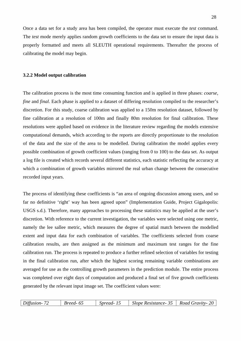
3.2.2 Model output calibration

The calibration process is the most time consuming function and is applied in three phases: coarse,

fine and final. Each phase is applied to a dataset of differing resolution compiled to the researcher’s

discretion. For this study, coarse calibration was applied to a 150m resolution dataset, followed by

fine calibration at a resolution of 100m and finally 80m resolution for final calibration. These

resolutions were applied based on evidence in the literature review regarding the models extensive

computational demands, which according to the reports are directly proportionate to the resolution

of the data and the size of the area to be modelled. During calibration the model applies every

possible combination of growth coefficient values (ranging from 0 to 100) to the data set. As output

a log file is created which records several different statistics, each statistic reflecting the accuracy at

which a combination of growth variables mirrored the real urban change between the consecutive

recorded input years.

The process of identifying these coefficients is “an area of ongoing discussion among users, and so

far no definitive ‘right’ way has been agreed upon” (Implementation Guide, Project Gigalopolis:

USGS s.d.). Therefore, many approaches to processing these statistics may be applied at the user’s

discretion. With reference to the current investigation, the variables were selected using one metric,

namely the lee sallee metric, which measures the degree of spatial match between the modelled

extent and input data for each combination of variables. The coefficients selected from coarse

calibration results, are then assigned as the minimum and maximum test ranges for the fine

calibration run. The process is repeated to produce a further refined selection of variables for testing

in the final calibration run, after which the highest scoring remaining variable combinations are

averaged for use as the controlling growth parameters in the prediction module. The entire process

was completed over eight days of computation and produced a final set of five growth coefficients

generated by the relevant input image set. The coefficient values were:

Diffusion- 72 Breed- 65 Spread- 15 Slope Resistance- 35 Road Gravity- 20

29 These parameters were then entered into the scenario file from which point prediction of growth

was initiated.

3.3 SLEUTH MODEL OUTPUT RESULTS

The final growth parameters derived through the calibration process were applied in the predict

function. The final urban layer for historic input now became the seed year from which the growth

variables were propagated. For this study the prediction was run from 1998 to 2040. SLEUTH

produced an output image of modelled urban extent for each year following the start or “seed” year

to the end year requested, thus a total of 42 output images were created. All 42 images are not

displayed in the text but rather, to highlight the changes in modelled urban extent, images were

selected at an interval of roughly ten years. If desired by the user the result images may be

simultaneously converted to an animation format through a supporting extension, Whirlgif, which is

supplied together with the SLEUTH download file. However, this function was not operational in

the modified MSDOS SLEUTH code, thus animations were created using IrfanView, a freeware

image viewer and editor. These animations can be viewed by accessing the compact disk supplied

in Appendix B and double-clicking the executable file Prediction_1998_to_2040. Watch the

simulation process over this time span enacted onscreen in a display that provides a powerful policy

presentation tool.

On the image displayed in Figure 3.6 all existing urban pixels derived from the seed year input are

displayed as yellow. Newly urbanized pixels as identified during the prediction process are assigned

colour based on the percentage probability of urbanization for that pixel. For the purposes of this

exercise the default colour settings for simulated pixels as prescribed in the scenario file were used

as listed in Table 3.1

Table 3.1: Default colour settings as applied by SLEUTH for denoting pixel probabilities for

urbanization.

Pixel colour probability for urbanization

Dark green 50% to 79%

Light green 80% to 94%

Dark red 95% to 100%

Yellow 100% (existing in seed year)

30 The images in Figures 3.8-3.10 are a selection of the result of the predict function applied through

the implementation of the growth rules and governed by the growth coefficients derived from the

calibration process. All of which is realistically controlled by the self modification function, as

discussed in the previous sections. This process is applied to each of the 42 years or ‘steps’ between

the ‘seed’ year and the end date for prediction.

Figure 3.6 displays the first year of the prediction run (after the seed year 1998) and reveals no trace

yet of pixel transitions from non-urban to urban. The modeling period is clearly too short to activate

noticeable growth simulation at this scale and furthermore may be accredited to the self

modification function as the model is acclimatized to the modeling environment. By 2010, however

(Figure 3.7), a dramatic change in the urban environment growth scenario has become evident;

expansion is clearly visible along urban fringes, most notably in the suburbs where vacant land

parcels are absorbed efficiently. This edge growth is attributed to that particular spread coefficient

and would fit exactly into the urban growth philosophy of the MSDF.

Figure 3.6: Modeling output result: Urban extent for the seed year 1999

Figure 3.7: Modeling output result: Urban extent for 2010

31 The first large scale evidence of high probability urban transition pixels become visible in the

patterns of Figure 3.8, where most of the peri-urban and rural nodes are displaying noticeable edge

growth as the city runs out of internal fill-up space by 2020. Thirty years down the line (Figure 3.9)

further densification becomes clearly visible in the city due to the high saturation of red pixels

starting to show in the image.

Figure 3.8: Modeling output result: Urban extent for 2020

Figure 3.9: Modeling output result: Urban extent for 2030

Rural nodes then become more prominent in the landscape as their edges expand. This expansion

retroactively increases the influence of the spread coefficient thereby compounding further growth.

Figure 3.10 shows the final image in the prediction sequence. With most land previously open to

development now absorbed, development creeps outward in classical urban sprawl configuration.

32

Figure 3.10: Modeling output result: Urban extent for 2040

Figure 3.11: The effect of the exclusion layer and year 2040 prediction

The outline of roads as development conduit magnets becomes noticeable as new developments

move along them. In the framed region A the eminent merging of several smaller nodes can be

observed, while framed region B shows strong contrast with a sharp urban edge realistically

enforced by the exclusion areas shown in Figure 3.11 of the zoned Rietvlei and adjacent

conservancies. Region B contains a predominantly agricultural region − the ‘soft’ target for all

natural urban expansion.

3.4 EVALUATION OF MODELING RESULTS

The results of the SLEUTH application exercise were evaluated in two ways: visually by comparing

various imagery, and numerically by recording the spatial coverage of various simulation classes on

these images. The results are discussed in the next two sections.

33

3.4.1 Visual evaluation of model results

In reviewing the model output, the growth pattern observed does not appear to be occurring at an

alarming rate. In fact, it would seem the growth pattern reflects the desired outcome of the

“Planning for Future Cape Town” initiative, as highlighted in Chapter 2. This is a highly positive

reflection on the Metropolitan planning practice in the era preceding the modeling exercise period,

because the model takes its growth cue from the preceding growth trend and extends that expansion

pace into the future. Growth appears controlled and directed with no alarming encroachment on

agricultural areas. Strong visual evidence supports both densification and the development of vacant

land in the city. Growth along the transport network between nodes is evident and the merging of a

number of satellite nodes reflects the desire for integration between existing nodes.

With visual inspection projecting a seemingly favourable image of Cape Town’s expansion, the

extent of growth also needs to be traced numerically. In an effort to evaluate the spatial extent of the

SLEUTH model prediction, the urban classified pixels in the output image for the year 2007 were

extracted and converted to a polygon theme in ESRI’s ArcGIS 9.1 software package. To create a

real-world urban extent layer for 2007, a shapefile of 2007 surveyed erven representing land parcels

registered within urban allotment areas (thus available to urban development) was acquired from

the Office of the Surveyor General (Cape Town). This shapefile was then clipped with the

Jurisdiction boundary of the Cape Metropolitan Council to extract only erven falling within the

demarcated study area. What remained after the clip was then compared with the excluded layer

produced for SLEUTH input. All erven greater than four hectares corresponding with an excluded

location were removed unless they showed signs of development such as a street layout. Finally, all

erven on the urban extremities were removed if they were greater than six hectares in size, unless

they showed evidence of development as in the previous step − this to account for smallholdings

and light agricultural functions which do not contribute to the developed urban extent. Figure 3.12

presents the result of the manipulation. The red pixels represent areas where the real world extent is

not ‘covered’ or correctly emulated by the urban model prediction and may be interpreted from the

map as areas of model under-estimation.

34

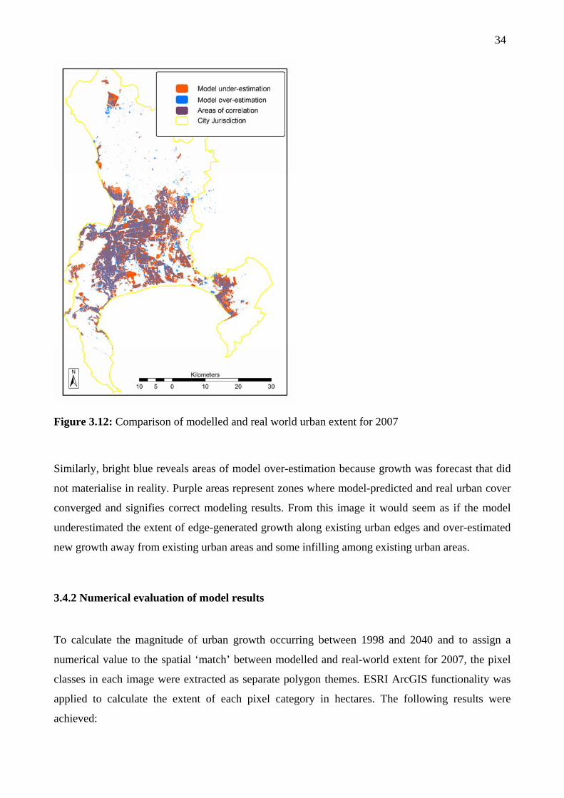
Figure 3.12: Comparison of modelled and real world urban extent for 2007

Similarly, bright blue reveals areas of model over-estimation because growth was forecast that did

not materialise in reality. Purple areas represent zones where model-predicted and real urban cover

converged and signifies correct modeling results. From this image it would seem as if the model

underestimated the extent of edge-generated growth along existing urban edges and over-estimated

new growth away from existing urban areas and some infilling among existing urban areas.

3.4.2 Numerical evaluation of model results

To calculate the magnitude of urban growth occurring between 1998 and 2040 and to assign a

numerical value to the spatial ‘match’ between modelled and real-world extent for 2007, the pixel

classes in each image were extracted as separate polygon themes. ESRI ArcGIS functionality was

applied to calculate the extent of each pixel category in hectares. The following results were

achieved:

35

3.4.2.1 Magnitude of predicted urban growth for 2040

A calculation of the total developed urban extent for 1998 produces a figure of 34483ha, and 42

years later the simulated total extent has increased to 76475ha of which 26465ha is attributed to

pixels in the range of 80% to 100% probability for urbanization. Table 3.2 represents the values

derived from SLEUTH output.

Table 3.2: Area calculations and comparisons for 1998 and 2040

Year Developed Area (seed)

Modelled Area Total Area 80% to 100% Probability

Probable area of urban extent

1998 34483ha - 34483ha - - 2040 34483ha 41992ha 76475ha 26465ha 60948ha

Thus, according to the calibrated growth coefficients, the urban developed area, consisting

primarily of the city of Cape Town, will have increased in area by 56.5% from 34483ha (1998) to

60948ha (2040). This figure is calculated using only the value for pixels in the 80% to 100%

urbanization probability range.

3.4.2.2 Spatial match of model to reality

A comparison of area calculations for the two 2007 themes reveals a 76% spatial overlap in

developed area, with the real world extent measuring 57163ha and the modelled extent measuring

43206ha. Based on these findings SLEUTH is judged by the research as a capable urban growth

prediction tool.

3.5 POLICY-ADJUSTED GROWTH PREDICTION

For the purpose of investigating the flexibility of the SLEUTH model to synthesise a scenario of

generic policy intervention, an exaggerated prediction run was performed. The urban growth

parameters for breed and spread were increased realistically as follows: the original calibration

derived values for breed was increased from 65 to 80 and for spread from 15 to 25. These new

values were assigned in an effort to simulate problematic urban sprawl and exaggerate the pressure

of development on agricultural land surrounding the urban areas. A modified exclusion layer was

36 then created which included a solid urban edge, completely surrounding the urban footprint of the

city. This was done to simulate an urban growth intervention policy, derived from the real-world

guidelines in Chapter 2. The policy scenario aimed to curb growth away from agricultural areas

using the urban edge as a no-go buffer zone, while relying on the pressure of expansion produced

by the same breed value to channel the growth along existing transport routes.

The resultant model prediction shown in Figure 3.13 attests to the absence of proper urban

containment policy, with urban sprawl consuming agricultural areas in uncontrolled fashion.

Figure 3.13: Exaggerated growth for year 2040 Figure 3.14: Exaggerated growth with urban edge modification for year 2040

Figure 3.14 reveals much the same growth pattern as the same variables were used for this

prediction, but subtle variations attributable to the urban edge buffer zone policy are clearly evident

in the resultant spatial pattern of predicted urbanisation.

3.6 INFORMATIVE AREAS IN CLOSE-UP

In order to better evaluate the efficacy of the previous model manipulations, the locations framed as

A and B in Figures 3.13. and 3.14, and that focus on a common area between the two scenarios,

37 were enlarged for closer scrutiny as seen in Figures 3.15 and 3.16. Locality B reflects the influence

of including an urban edge as a solid barrier to urban expansion. The most obvious variation is

viewed in the south west corner of each locality. In Locality A an amalgamation of nodes occurring

on the edge of the city extent is observed. In Locality B the same nodes show little or no evidence

of urbanization. Upon closer inspection one observes a broad belt of no development that accurately

outlines the position of an urban edge. However a comparison of the north eastern corner reveals

that the boundary did little to divert or suppress urbanization beyond its location in model space.

Figure 3.15: Enlarged view of a problem area under the exaggerated growth scenario

Figure 3.16: Enlarged view of a problem area under the urban edge modification scenario

From these observations it is deduced that a) one is able to produce high impact emergency

scenarios by exaggerating growth values and b) it is possible to influence the growth pattern,

however these influences will be localized to the immediate vicinity of the controlling factor. Thus

to effectively redirect or control growth one would need to apply a blanket control such as

expanding the excluded layer to include all identified land to be preserved. For the urban edge

scenario to have produced the desired results the exclusion layer would have to include all areas

38 falling beyond the edge itself and road growth would have to be accommodated or directed by

providing growth channels in the hard exclusion layer.

In summary, it is clear that the SLEUTH model does allow a high level of user manipulation to

approximate real word urban expansion trends or, on the other hand to simulate the effect of the

measures to be expected by interventionist policy measures from the planning and political

authorities of a major metropolis.

39

CHAPTER 4 SUMMARY, CONCLUSIONS AND RECOMMENDATIONS

In this final chapter the salient research results are summarised and the work is evaluated in terms

of its contribution to practical urban governance on the one hand and academic enquiry on the other

hand. In conclusion some recommendations for model application are made and the future

generations of Geography researchers are provided with suggestions for future research.

4.1 SUMMARY OF RESEARCH RESULTS

Since the research was driven by the concise objectives set in Section 1.4.2, these may now be

revisited to summarise the results. Objective 1 was to identify strategies currently formulated by the

metropolitan government to manage the extent and nature of urban growth in Cape Town. In

consequence, in Chapter 2 the MSDF was discussed as a guideline for directing urban planning

initiatives. The document identified four spatial planning goals of the metropolitan government,

namely; to provide direction for physical growth at metropolitan scale; to provide spatial direction

to Reconstruction and Development projects (RDP); to provide a framework for co-ordinated action

between the public, private and community sectors; and to provide the basis for the preparation of

policies, programmes and development strategies at local and metropolitan levels, following which,

the guidelines and strategies for achieving these goals were identified. Secondly, the State of Cape

Town Report (City of Cape Town 2006) was briefly discussed. The document served to present

extensive proposal and growth options for the “Planning for Future Cape Town” initiative for which

five strategic areas of action were recognised being; the protection of natural assets and

development of a quality open space system; the redefining and development of a new economic

backbone for the city; development of an equitable pattern of access; the development of an

integrated city development path; and developing a new pattern of special places. The research thus

delivered positively on the first objective.

Objective 2, largely also covered in Chapter 2, set out to explore and evaluate the feasibility of

cellular automata and the SLEUTH software in particular as a modeling framework tool to simulate

urban growth in support of growth management policy. It found that this modeling tool had been

successfully implemented in a range of locations mainly in the developed world to model urban

expansion. The model was praised for its adaptability, especially in the modeling of policy

scenarios, the researchers also found the model to be considerably user friendly. A common concern

however, was the models intensive computing demands on hardware. This survey also included

40 obtaining and describing the technical procedures and requirements of the SLEUTH model

documented in the second part of Chapter 2. It is felt that the report will provide sufficient

particulars concerning model application to inform and encourage future users, operational and

academic, in the use of the software for urban growth and related modeling endeavours.

In Chapter 3 the third objective, namely to practically implement and evaluate the performance and

efficacy of the SLEUTH software to model future urban expansion in Cape Town was achieved

successfully. The model was calibrated using several data sets of historic urban extent as well as an

exclusion layer, transport layers and slope data. The growth parameters derived from this process

were applied to project the growth of the city from 1998 to 2040. The results show a realistic

pattern of growth and expansion for the city, fortified by the model’s adherence to outcomes

identified in the MSDF document discussed in Chapter 2. Further analysis of the forecast for the

period 1998 to 2040 revealed an increase in the area of the urban footprint by at least 56.5% when

calculated conservatively using only pixels in the 80% to 100% probability for urbanization range.

Furthermore, a spatial comparison of modelled urban extent and real-world urban extent for the

output year of 2007 revealed a spatial match of 76%. In order to investigate the flexibility of the

SLEUTH model to synthesise a scenario of generic policy intervention, an exaggerated prediction

run was performed in which the growth parameters were realistically altered. These new values

were assigned in an effort to simulate problematic urban sprawl and exaggerate the pressure of

development on agricultural land surrounding the urban areas. It was deduced that a) one is able to

produce high impact emergency scenarios by exaggerating growth values and b) it is possible to

influence the growth pattern, however these influences will be localized to the immediate vicinity of

the controlling factor.

In conclusion SLEUTH was judged by the research as a capable urban growth prediction tool, not

only for propagating the subject city’s unique growth trends but also for its allowance of user

manipulation to approximate real word urban expansion trends or, on the other hand to simulate the

effect of the measures to be expected by interventionist policy measures from the planning and

political authorities of a major metropolis.

4.2 THE ACADEMIC AND OPERATIONAL VALUE OF THE RESEARCH

SLEUTH not only functions as a tool for forecasting urban growth into the future, but allows the

user to gain an insight into the historical growth patterns that resulted in the city’s present tense. It

is this graphic visualisation of the past together with a glimpse into their future that will allow both

41 geographers and historians to “rewind” what has past, and planners to make more informed

strategic decisions. By considering the output of these forecasts city managers are able to identify

areas of concern for the future and implement preventative or controlling factors in advance.

Infrastructure and services may be planned or upgraded in advance of demand. It is this function of

SLEUTH which is of greatest value.

4.3 RECOMMENDATIONS FOR MODEL APPLICATION

A study of the literature revealed a general consensus as to the ease of model application, however

in the experience of the research it is advisable to have a good understanding of the command

driven computing environment and a basic understanding of scripting and basic c# programming

language. Solid knowledge of GIS software functionality is strongly advised as this is imperative

for not only preparation and conversion of data for compatibility with SLEUTH but also post

processing and analysis of SLEUTH output. Finally, SLEUTH is memory intensive and it is

recommended that the application be executed on a computing system with high specifications.

Larger study areas will require more computing power.

4.4 RECOMMENDATIONS FOR FUTURE RESEARCH

A thorough data set of the City of Cape Town was available for the research; this may not

necessarily be the case for all cities and regions. The process of constructing a historic database

where such data is unavailable will be time consuming and utterly reliant on the availability of

historic image datasets from which urban footprints can be extracted.

Though the model may be viewed as a valuable planning tool it remains just that, a prediction tool,

reliant on interpretation by experienced professionals. Model output is a forecast of the urban/ non-

urban state of a pixel based on basic factors of slope influence and road gravity. As such,

phenomena such as rural-urban migration patterns and socio-economic influences are not addressed,

a major contributing factor in the growth and transformation of the city-scape. This however, should

not limit the further application of SLEUTH output in other modeling environments such as

modeling the effect of future urban extent on drainage patterns or local micro-climates.

This research is the first evidence of a SLEUTH application in the South African context; as such

the topic invites many opportunities for further investigation. In closing the research suggests the

following possibilities:

42

- The application of SLEUTH to investigate urban growth in other regions of South Africa;

- To model growth for the country in its entirety;

- To re-explore and refine the simulation of policy scenarios in the model;

- An investigation into the influence of data resolution in the SLEUTH modeling

environment;

- Exploring the various methods of gathering data for the model;

- Exploring the influence of varying temporal differences between historic input layers on

calibration results;

- Application of SLEUTH output with other modeling environments.

43

REFERENCES

Barredo JI, Kasanko M, McCormick N & Lavalle C 2003. Modeling dynamic spatial processes: simulation of urban future scenarios through cellular automata. Landscape and Urban Planning 64: 145-160. [online], Available from: http://www.elsevier.com/locate/landurbplan/ [Accessed 22 March 2005].

Batty M 1997. Cellular automata and urban form: a primer. Journal of the American Planning Association 63, 2: 266-275. [online], Available from: http://www.weblinks3.epnet.com/citation.asp/ [Accessed 24 March 2005].

Candau J 2000. Calibrating a cellular automaton model of urban growth in a timely manner. 4th International Conference on Integrating GIS and Environmental Modeling (GIS/EM4): problems, prospects and research needs, Alberta, Canada. [online], Available from: http://www.geog.ucsb.edu/ [Accessed 21 March 2005].

Candau J, Rasmussen S & Clarke KC 2000. A coupled cellular automaton model for land use/land cover dynamics. 4th International Conference on Integrating GIS and Environmental Modeling (GIS/EM4): problems, prospects and research needs, Alberta, Canada. [online], Available from: http://www.geog.ucsb.edu/ [Accessed 21 March 2005].

Cheng J & Masser I 2004. Understanding spatial and temporal processes of urban growth: Cellular automata modeling. Environment and Planning B: Planning and Design 31: 167-194. [online], Available from: http://www.envplan.com [Accessed 22 March 2005].

City of Cape Town 2006. State of Cape Town Report 2006: Development issues in Cape Town. Cape Town, City of Cape Town.

Clarke KC (s.d.) Land transition modeling with deltatrons. Santa Barbara: University of California, Department of Geography. [online], Available from: http://geog.ucsb.edu/~kclarke [Accessed 21 March 2005].

Clarke KC & Gaydos LJ 1998. Loose-coupling a cellular automaton model and GIS: Long-term urban growth prediction for San Francisco and Washington/Baltimore. International Journal of Geographical Information Science 12, 7: 699-714. [online], Available from: http://www.tandf.co.uk/journals/tf/ [Accessed 23 March 2005].

Compas E & Sugumaran R 2004. Urban growth modeling on the web: A decision support tool for community planners. Papers of the Applied Geography Conference (s.l.). [online], Available from: http://www.champlain.geography.wisc.edu/~educompas/ [Accessed 21 March 2005].

Davies, DH 1963. Land use in Central Cape Town. Doctoral dissertation. Cape Town: University of Cape Town.

Goldstein NC, Candau JT & Clarke KC 2004. Approaches to simulating the “March of Bricks and Mortar”. Computers, Environment and Urban Systems 28: 125-147. [online], Available from: http://www.elsevier.com/locate/landurbplan/ [Accessed 22 March 2005].

Herold M, Goldstein NC & Clarke KC 2002. The spatiotemporal form of urban growth: measurement, analysis and modeling. Santa Barbara, University of California, Department of Geography. [online], Available from: http:// www.sciencedircect.com. [Accessed 25 March 2005].

Herold M, Menz G & Clarke KC (s.d.). Remote sensing and urban growth models - demands and perspectives. Santa Barbara: University of California, Department of Geography. [online], Available from: http://geog.ucsb.edu/~mherold/herold_menz_clarke. [Accessed 21 March 2005].

Jantz CA, Goetz SJ & Shelley MK 2003. Using the SLEUTH urban growth model to simulate the impacts of future policy scenarios on urban land use in the Baltimore-Washington metropolitan area. Environment and Planning B: Planning and Design 30: 251-271. [online], Available from: http://www.envplan.com [Accessed 22 March 2005].

Kaiser E, Godschalk D & Chapin Jr SF 1995. Urban land use planning. Urbana, IL: University of Illinois.

44 Klostermann RE 1999. The what if? Collaborative planning support system. Environment and

Planning. B, Planning and Design 26: 393– 408. Kocabas V & Dragicevic S 2004. Sensitivity analysis of a GIS- based cellular automata model.

Spatial Analysis Modeling Laboratory. [online], Available from: http://www.isprs.org/istanbul 2004/comm4/papers/321.pdf [Accessed 21 March 2005].

Li X & Gar-On Yeh A 2000. Modeling sustainable urban development by the integration of constrained cellular automata and GIS. International Journal of Geographical Information Science 14, 2: 131-152. [online], Available from: http://www.tandf.co.uk/journals/tf/ [Accessed 23 March 2005].

Masser I 2001. Managing our urban future: The role of remote sensing and geographic information systems. Habitat International 25: 503-512. [online] Available from: http://www.elsevier.com/locate/habitatint [Accessed 22 March 2005].

Metropolitaanse Ruimtelike Ontwikkelingsraamwerk, 1996. ‘n Gids vir ruimtelike ontwikkeling in die Kaapse Metropolitaanse Funksionele Streek: Tegniese verslag April 2006.

United States Geological Survey (USGS) s.d. Project Gigalopolis. [online], Available from: http:/www.ncgia.ucsb.edu/projects/gig [Accessed 15 September 2005].

Silva EA & Clarke KC 2002. Calibration of the SLEUTH urban growth model for Lisbon and Porto, Portugal. Computers, Environment and Urban Systems 26: 525-552. [online], Available from: http://www.elsevier.com/locate/landurbplan/. [Accessed 22 March 2005].

Smith L (s.d.) The urban political ecology of water in Cape Town, South Africa (s.n.). [online], Available from: http://www.queensu.ca/msp/pages/Project_Publications [Accessed 27 May 2007].

Torrens PM & O’Sullivan D 2001. Editorial: Cellular automata and urban simulation: Where do we go from here? Environment and Planning B: Planning and Design 28: 163-168. [online], Available from: http://www.envplan.com [Accessed 22 March 2005].

Van der Merwe JH 1980. Ontwikkeling en struktuur van die landelik-stedelike oorgangsone van Kaapstad. Masters thesis. Stellenbosch: Stellenbosch University, Department of Geography.

Wilson E, Hurd J & Civco D 2002. Development of a model to quantify and map urban growth. ASPRS-ACSM Annual Conference and FIG XXII Congress, Connecticut: University of Connecticut. [online], Available from: http://www.resac.uconn.edu/publications/tech-papers/ [Accessed 24 March 2005].

Yang X & Lo CP 2003. Modeling urban growth and landscape changes in the Atlanta metropolitan area. International Journal of Geographical Information Science 17, 5: 463-488. [online], Available from: http://www.tandf.co.uk/journals/tf/ [Accessed 23 March 2005].

45

APPENDICES A. The SLEUTH scenario file B Animation of prediction for growth coefficients derived from historic data

calibration

46

APPENDIX A: THE SLEUTH SCENARIO FILE AS PROVIDED WITH THE

PROGRAMME DOWNLOAD

(Note to users: this file is used for both calibration runs and forecasting runs, as such, it is

constantly edited and amended. For this reason it is recommended that this file be kept as a

reference for default settings.)

# FILE: 'scenario file' for SLEUTH land cover transition model # (UGM v3.0 beta) # Comments start with # # # I. Path Name Variables # II. Running Status (Echo) # III. Output ASCII Files # IV. Log File Preferences # V. Working Grids # VI. Random Number Seed # VII. Monte Carlo Iteration #VIII. Coefficients # A. Coefficients and Growth Types # B. Modes and Coefficient Settings # IX. Prediction Date Range # X. Input Images # XI. Output Images # XII. Colortable Settings # A. Date_Color # B. Non-Landuse Colortable # C. Land Cover Colortable # D. Growth Type Images # E. Deltatron Images #XIII. Self Modification Parameters # I. PATH NAME VARIABLES # INPUT_DIR: relative or absolute path where input image files are # located. # OUTPUT_DIR: relative or absolute path where all output files will # be located. # WHIRLGIF_BINARY: relative path to 'whirlgif' gif animation program. # These must be compiled before execution. INPUT_DIR=../Input/demo200/ OUTPUT_DIR=../Output/ WHIRLGIF_BINARY=../Whirlgif/whirlgif # II. RUNNING STATUS (ECHO) # Status of model run, monte carlo iteration, and year will be # printed to the screen during model execution. ECHO(YES/NO)=yes # III. Output Files # INDICATE TYPES OF ASCII DATA FILES TO BE WRITTEN TO OUTPUT_DIRECTORY. # # COEFF_FILE: contains coefficient values for every run, monte carlo # iteration and year. # AVG_FILE: contains measured values of simulated data averaged over # monte carlo iterations for every run and control year. # STD_DEV_FILE: contains standard deviation of averaged values # in the AVG_FILE. # MEMORY_MAP: logs memory map to file 'memory.log'

47 # LOGGING: will create a 'LOG_#' file where # signifies the processor # number that created the file if running code in parallel. # Otherwise, # will be 0. Contents of the LOG file are # described below. WRITE_COEFF_FILE(YES/NO)=yes WRITE_AVG_FILE(YES/NO)=yes WRITE_STD_DEV_FILE(YES/NO)=yes WRITE_MEMORY_MAP(YES/NO)=no LOGGING(YES/NO)=YES # IV. Log File Preferences # INDICATE CONTENT OF LOG_# FILE (IF LOGGING == ON). # LANDCLASS_SUMMARY: (if landuse is being modelled) summary of input # from 'landuse.classes' file # SLOPE_WEIGHTS(YES/NO): annual slope weight values as affected # by slope_coeff # READS(YES/NO)= notes if a file is read in # WRITES(YES/NO)= notes if a file is written # COLORTABLES(YES/NO)= rgb lookup tables for all colortables generated # PROCESSING_STATUS(0:off/1:low verbosity/2:high verbosity)= ???? # TRANSITION_MATRIX(YES/NO)= pixel count and annual probability of # land class transitions # URBANIZATION_ATTEMPTS(YES/NO)= number of times an attempt to urbanize # a pixel occurred # INITIAL_COEFFICIENTS(YES/NO)= initial coefficient values for # each monte carlo # BASE_STATISTICS(YES/NO)= measurements of urban control year data # DEBUG(YES/NO)= data dump of igrid object and grid pointers # TIMINGS(0:off/1:low verbosity/2:high verbosity)= time spent within # each module. If running in parallel, LOG_0 will contain timing for # complete job. LOG_LANDCLASS_SUMMARY(YES/NO)=yes LOG_SLOPE_WEIGHTS(YES/NO)=no LOG_READS(YES/NO)=no LOG_WRITES(YES/NO)=no LOG_COLORTABLES(YES/NO)=NO LOG_PROCESSING_STATUS(0:off/1:low verbosity/2:high verbosity)=1 LOG_TRANSITION_MATRIX(YES/NO)=yes LOG_URBANIZATION_ATTEMPTS(YES/NO)=no LOG_INITIAL_COEFFICIENTS(YES/NO)=no LOG_BASE_STATISTICS(YES/NO)=yes LOG_DEBUG(YES/NO)= no LOG_TIMINGS(0:off/1:low verbosity/2:high verbosity)=1 # V. WORKING GRIDS # The number of working grids needed from memory during model execution is # designated up front. This number may change depending upon modes. If # NUM_WORKING_GRIDS needs to be increased, the execution will be exited and # an error message will be written to the screen and to 'ERROR_LOG' in the # OUTPUT_DIRECTORY. If the number may be decreased an optimal number will # be written to the end of the LOG_0 file. NUM_WORKING_GRIDS=5 # VI. RANDOM NUMBER SEED # This number initializes the random number generator. This seed will be used # to initialize each model run. RANDOM_SEED=47392074 # VII. MONTE CARLO ITERATIONS # Each model run may be completed in a monte carlo fashion. # For CALIBRATION or TEST mode, measurements of simulated data will be taken # for years of known data, and averaged over the number of monte carlo # iterations. These averages are written to the "avg.log" file, and the

48 # associated standard deviation is written to the "std_dev.log" file. The # averaged values are compared to the known data, and a Pearson correlation # coefficient measure is calculated and written to the "control.stats.log" # file. The input per run may be associated across files using the 'index' # number in the files' first column. # MONTE_CARLO_ITERATIONS=2

# VIII. COEFFICIENTS # The coefficients affect how the growth rules are applied to the data. # For additional information see our publications and PROJECT # GIGALOPOLIS web site (www.ncgia.ucsb.edu/project/gig/About/gwCoef.htm) # and (www.ncgia.ucsb.edu/project/gig/About/gwRules.htm). # A. COEFFICIENTS AND GROWTH TYPES # DIFFUSION: affects SPONTANEOUS GROWTH and search distance along the # road network as part of ROAD INFLUENCED GROWTH. # BREED: NEW SPREADING CENTER probability and affects number of ROAD # INFLUENCED GROWTH attempts. # SPREAD: the probability of ORGANIC GROWTH from established urban pixels # occurring. # SLOPE_RESISTANCE: affects the influence of slope to urbanization. As # value increases, the ability to urbanize steepening # slopes decreases. # ROAD_GRAVITY: affects the outward distance from a selected pixel for # which a road pixel will be searched for as part of ROAD # INFLUENCED GROWTH. # # B. MODES AND COEFFICIENT SETTINGS # TEST: TEST mode will perform a single run through the historical # data using the CALIBRATION_*_START values to initialize # growth, complete the MONTE_CARLO_ITERATIONS, and then conclude # execution. GIF images of the simulated urban growth will be # written to the OUTPUT_DIRECTORY. # CALIBRATE: CALIBRATE will perform monte carlo runs through the # historical data using every combination of the coefficient # values indicated. The CALIBRATION_*_START coefficient # values will initialize the first run. A coefficient # will then be increased by its _STEP value, and # another run performed. This will be repeated for all possible # permutations of given ranges and increments until the # _STOP value is reached or exceeded. # PREDICTION: PREDICTION will perform a single run, a # NUMBER_OF_ITERATIONS times in monte carlo fashion, using # the PREDICTION_*_BEST_FIT values for initialization.

CALIBRATION_DIFFUSION_START= 0 CALIBRATION_DIFFUSION_STEP= 25 CALIBRATION_DIFFUSION_STOP= 100

CALIBRATION_BREED_START= 0 CALIBRATION_BREED_STEP= 25 CALIBRATION_BREED_STOP= 100

CALIBRATION_SPREAD_START= 0 CALIBRATION_SPREAD_STEP= 25 CALIBRATION_SPREAD_STOP= 100

CALIBRATION_SLOPE_START= 0 CALIBRATION_SLOPE_STEP= 25 CALIBRATION_SLOPE_STOP= 100

49 CALIBRATION_ROAD_START= 0 CALIBRATION_ROAD_STEP= 25 CALIBRATION_ROAD_STOP= 100

PREDICTION_DIFFUSION_BEST_FIT= 20 PREDICTION_BREED_BEST_FIT= 20 PREDICTION_SPREAD_BEST_FIT= 20 PREDICTION_SLOPE_BEST_FIT= 2 PREDICTION_ROAD_BEST_FIT= 20 # IX. PREDICTION DATE RANGE # The urban and road images used to initialize growth during # prediction are those with dates equal to, or greater than, # the PREDICTION_START_DATE. If the PREDICTION_START_DATE is greater # than any of the urban dates, the last urban file on the list will be # used. Similarly, if the PREDICTION_START_DATE is greater # than any of the road dates, the last road file on the list will be # used. The prediction run will terminate at PREDICTION_STOP_DATE. # PREDICTION_START_DATE=1990 PREDICTION_STOP_DATE=2010 # X. INPUT IMAGES # The model expects grayscale, GIF image files with file name # format as described below. For more information see our # PROJECT GIGALOPOLIS web site: # (www.ncgia.ucsb.edu/project/gig/About/dtInput.htm). # # IF LAND COVER IS NOT BEING MODELED: Remove or comment out # the LANDUSE_DATA data input flags below. # # < > = user selected fields # [< >] = optional fields # # Urban data GIFs # format: <location>.urban.<date>.[<user info>].gif # # URBAN_DATA= demo200.urban.1930.gif URBAN_DATA= demo200.urban.1950.gif URBAN_DATA= demo200.urban.1970.gif URBAN_DATA= demo200.urban.1990.gif # # Road data GIFs # format: <location>.roads.<date>.[<user info>].gif # ROAD_DATA= demo200.roads.1930.gif ROAD_DATA= demo200.roads.1950.gif ROAD_DATA= demo200.roads.1970.gif ROAD_DATA= demo200.roads.1990.gif # # Landuse data GIFs # format: <location>.landuse.<date>.[<user info>].gif # #LANDUSE_DATA= demo200.landuse.1930.gif #LANDUSE_DATA= demo200.landuse.1990.gif # # Excluded data GIF # format: <location>.excluded.[<user info>].gif # EXCLUDED_DATA= demo200.excluded.gif # # Slope data GIF

50 # format: <location>.slope.[<user info>].gif # SLOPE_DATA= demo200.slope.gif # # Background data GIF # format: <location>.hillshade.[<user info>].gif # BACKGROUND_DATA= demo200.hillshade.gif # XI. OUTPUT IMAGES # WRITE_COLOR_KEY_IMAGES: Creates image maps of each colortable. # File name format: 'key_[type]_COLORMAP' # where [type] represents the colortable. # ECHO_IMAGE_FILES: Creates GIF of each input file used in that job. # File names format: 'echo_of_[input_filename]' # where [input_filename] represents the input name. # ANIMATION: if whirlgif has been compiled, and the WHIRLGIF_BINARY # path has been defined, animated gifs beginning with the # file name 'animated' will be created in PREDICT and # CALIBRATE mode. WRITE_COLOR_KEY_IMAGES(YES/NO)=yes ECHO_IMAGE_FILES(YES/NO)=yes ANIMATION(YES/NO)= yes # XII. COLORTABLE SETTINGS # A. DATE COLOR SETTING # The date will automatically be placed in the lower left corner # of output images. DATE_COLOR may be designated in with red, green, # and blue values (format: <red_value, green_value, blue_value> ) # or with hexadecimal beginning with '0X' (format: <0X######> ). #default DATE_COLOR= 0XFFFFFF white DATE_COLOR= 0XFFFFFF #white

# B. URBAN (NON-LANDUSE) COLORTABLE SETTINGS # 1. URBAN MODE OUTPUTS # TEST mode: Annual images of simulated urban growth will be # created using SEED_COLOR to indicate urbanized areas. # CALIBRATE mode: Images will not be created. # PREDICT mode: Annual probability images of simulated urban # growth will be created using the PROBABILITY # _COLORTABLE. The initializing urban data will be # indicated by SEED_COLOR. # # 2. COLORTABLE SETTINGS # SEED_COLOR: initializing and extrapolated historic urban extent # WATER_COLOR: BACKGROUND_DATA is used as a backdrop for simulated # urban growth. If pixels in this file contain the # value zero (0), they will be filled with the color # value in WATER_COLOR. In this way, major water bodies # in a study area may be included in output images. # #SEED_COLOR= 0XFFFF00 #yellow SEED_COLOR= 255, 255, 0 #yellow WATER_COLOR= 0X0000FF # blue

# 3. PROBABILITY COLORTABLE FOR URBAN GROWTH # For PREDICTION, annual probability images of urban growth # will be created using the monte carlo iterations. In these # images, the higher the value, the more likely urbanizaion is. # In order to interpret these 'continuous' values more easily # they may be color classified by range. #

51 # If 'hex' is not present then the range is transparent. # The transparent range must be the first on the list. # The max number of entries is 100. # PROBABILITY_COLOR: a color value in hexadecimal that indicates a # probability range. # low/upper: indicate the boundaries of the range. # # low, upper, hex, (Optional Name) PROBABILITY_COLOR= 0, 50, , #transparent PROBABILITY_COLOR= 50, 60, 0X005A00, #0, 90,0 PROBABILITY_COLOR= 60, 70, 0X008200, #0,130,0 PROBABILITY_COLOR= 70, 80, 0X00AA00, #0,170,0 PROBABILITY_COLOR= 80, 90, 0X00D200, #0,210,0 PROBABILITY_COLOR= 90, 95, 0X00FF00, #0,255,0 PROBABILITY_COLOR= 95, 100, 0X8B0000, #dark red

# C. LAND COVER COLORTABLE # Land cover input images should be in grayscale GIF image format. # The 'pix' value indicates a land class grayscale pixel value in # the image. If desired, the model will create color classified # land cover output. The output colortable is designated by the # 'hex/rgb' values. # pix: input land class pixel value # name: text string indicating land class # flag: special case land classes # URB - urban class (area is included in urban input data # and will not be transitioned by deltatron) # UNC - unclass (no data areas in image) # EXC - excluded (land class will be ignored by deltatron) # hex/rgb: hexadecimal or rgb (red, green, blue) output colors # # pix, name, flag, hex/rgb, #comment LANDUSE_CLASS= 0, Unclass , UNC , 0X000000 LANDUSE_CLASS= 1, Urban , URB , 0X8b2323 LANDUSE_CLASS= 2, Agric , , 0Xffec8b #pale yellow LANDUSE_CLASS= 3, Range , , 0Xee9a49 #tan LANDUSE_CLASS= 4, Forest , , 0X006400 LANDUSE_CLASS= 5, Water , EXC , 0X104e8b LANDUSE_CLASS= 6, Wetland , , 0X483d8b LANDUSE_CLASS= 7, Barren , , 0Xeec591 LANDUSE_CLASS= 8, Tundra , , 0X323232 LANDUSE_CLASS= 9, Ice&Sno , , 0XFFFFFF # D. GROWTH TYPE IMAGE OUTPUT CONTROL AND COLORTABLE # # From here you can control the output of the Z grid # (urban growth) just after it is returned from the spr_spread() # function. In this way it is possible to see the different types # of growth that have occurred. # # VIEW_GROWTH_TYPES(YES/NO) provides an on/off # toggle to control whether the images are generated. # # GROWTH_TYPE_PRINT_WINDOW provides a print window # to control the amount of images created. # format: <start_run>,<end_run>,<start_monte_carlo>, # <end_monte_carlo>,<start_year>,<end_year> # for example: # GROWTH_TYPE_PRINT_WINDOW=run1,run2,mc1,mc2,year1,year2 # so images are only created when # run1<= current run <=run2 AND # mc1 <= current monte carlo <= mc2 AND # year1 <= current year <= year2

52 # # 0 == first VIEW_GROWTH_TYPES(YES/NO)=NO GROWTH_TYPE_PRINT_WINDOW=0,0,0,0,1995,2020 PHASE0G_GROWTH_COLOR= 0xff0000 # seed urban area PHASE1G_GROWTH_COLOR= 0X00ff00 # diffusion growth PHASE2G_GROWTH_COLOR= 0X0000ff # NOT USED PHASE3G_GROWTH_COLOR= 0Xffff00 # breed growth PHASE4G_GROWTH_COLOR= 0Xffffff # spread growth PHASE5G_GROWTH_COLOR= 0X00ffff # road influenced growth #************************************************************ # # E. DELTATRON AGING SECTION # # From here you can control the output of the deltatron grid # just before they are aged # # VIEW_DELTATRON_AGING(YES/NO) provides an on/off # toggle to control whether the images are generated. # # DELTATRON_PRINT_WINDOW provides a print window # to control the amount of images created. # format: <start_run>,<end_run>,<start_monte_carlo>, # <end_monte_carlo>,<start_year>,<end_year> # for example: # DELTATRON_PRINT_WINDOW=run1,run2,mc1,mc2,year1,year2 # so images are only created when # run1<= current run <=run2 AND # mc1 <= current monte carlo <= mc2 AND # year1 <= current year <= year2 # # 0 == first VIEW_DELTATRON_AGING(YES/NO)=NO DELTATRON_PRINT_WINDOW=0,0,0,0,1930,2020 DELTATRON_COLOR= 0x000000 # index 0 No or dead deltatron DELTATRON_COLOR= 0X00FF00 # index 1 age = 1 year DELTATRON_COLOR= 0X00D200 # index 2 age = 2 year DELTATRON_COLOR= 0X00AA00 # index 3 age = 3 year DELTATRON_COLOR= 0X008200 # index 4 age = 4 year DELTATRON_COLOR= 0X005A00 # index 5 age = 5 year # XI.SELF-MODIFICATION PARAMETERS # SLEUTH is a self-modifying cellular automata. For more information # see our PROJECT GIGALOPOLIS web site: # (www.ncgia.ucsb.edu/project/gig/About/gwSelfMod.htm) # and publications (and/or grep 'self modification' in code). ROAD_GRAV_SENSITIVITY=0.01 SLOPE_SENSITIVITY=0.1 CRITICAL_LOW=0.97 CRITICAL_HIGH=1.03 #CRITICAL_LOW=0.0 #CRITICAL_HIGH=10000000000000.0 CRITICAL_SLOPE=15.0 BOOM=1.1 BUST=0.9

53

APPENDIX B: ANIMATION OF PREDICTION FOR GROWTH COEFFICIENTS

DERIVED FROM HISTORIC DATA CALIBRATION (Electronic version on CD in cover

sleeve)

Directions: Double-click the executable file Prediction_1998_to_2040