The Shortest Route - VU · large amount of route planning software available, ... 2.7 ALT algorithms ... algorithms is given. In Chapter 3 a number of other route planners are discussed

The Shortest Route

Developing an online bicycle route planner for the Netherlands

Wouter Pepping

BMI Paper VU University Amsterdam

April 2009

Supervisor: Peter Kampstra Second reader: Sandjai Bhulai

B M

I

The Shortest Route: Developing a bicycle route planner for the Netherlands April 2009

2 / 40


3 / 40

Preface

This paper was written as an assignment for my Master in Business Mathematics &

Informatics. The goal of the assignment is to write a paper on a research subject

combining the business, mathematics and computer science aspects of the Master.

During my search for a suitable subject, Peter Kampstra mentioned that while there was a

large amount of route planning software available, the Netherlands is still lacking an

online bicycle route planner. Sure, some stand alone route planners have the option to

plan bicycle routes and some provinces offer their own bicycle route planner, but an

online planner covering all of the country is still not available.

Having encountered this issue myself in the past (I ended up taking the bus), my interest

was awakened. Would it be possible to implement a bicycle route planner for the

Netherlands with acceptable response times within the timeframe of a month? I took on

the challenge and this paper presents the results of the research that I did, the choices that

I made for the implementation and the resulting product.

I would like to thank Peter for proposing the subject and for all his useful suggestions as

my supervisor. Furthermore, thanks to Sandjai Bhulai for agreeing to be the second

reader, despite his busy schedule. And last but not least my thanks go out to Annemieke

van Goor for not resting until I finally got started on the project.

Wouter Pepping,

March 2009.


4 / 40


5 / 40

Summary

In the past few years, route planners have rapidly become a part of every day life. All

route planners depend on a routing algorithm to calculate the shortest or fastest route

from a starting point to a destination. However, there is not one best algorithm that is

used everywhere. Each route planner uses its own algorithm, based on a number of

considerations: calculation time, preprocessing time, memory usage, complexity and

whether the solution is optimal or suboptimal.

The most well-known routing algorithm is Dijkstra’s algorithm. However, in terms of

speed and memory usage, Dijkstra cannot compete with more recent methods. A* and

bidirectional search try to improve Dijkstra’s performance by only changing the routing

algorithm, which results in small speedups. Geometric pruning, ALT algorithms and the

multi-level approach use preprocessing to analyze the data. While adding preprocessing

time and increasing complexity, these methods can greatly reduce calculation times, even

up to a factor 1,000. Moreover, most methods can be combined to achieve even greater

speedups. This means calculation times can be decreased to a few milliseconds. With

calculation times this small, this will no longer form a bottleneck, but overhead like

transmitting the data over a network or displaying the route will. For this reason, recent

research indicates it is no longer interesting to accept suboptimal solutions in order to

decrease calculation times.

During the course of the project, a study on existing route planners was performed. This

study confirmed that there still is no Dutch route planner that offers decent support for

planning bicycle routes and covers the entire Netherlands. The Dutch route planners that

do offer the option to plan bicycle routes do not have bicycle paths in their data, resulting

in inaccurate results.

Using the gained knowledge about routing algorithms, an online bicycle route planner

was implemented for the Netherlands. In order to achieve acceptable processing times,

the A* algorithm is used in combination with a specific data structure known as a

Fibonacci heap. Using this method, even the longest routes can be calculated within

acceptable time, while short routes take only a few milliseconds.

The speedup of A* over Dijkstra is impressive for shorter routes, but almost negligible

for routes that cross the entire country. The most probably cause for this effect is that the

borders of the dataset prevent unnecessary expansion of Dijkstra’s search space for the

latter.


6 / 40


7 / 40

Contents

1 Introduction ........................................................................................................... 9

2 Literature ............................................................................................................. 10 2.1 Shortest path problem ..................................................................................... 10

2.2 LP model ......................................................................................................... 11

2.3 Dijkstra ............................................................................................................ 12

2.4 A* .................................................................................................................... 14

2.5 Bidirectional search ........................................................................................ 17

2.6 Geometric pruning using bounding-boxes ...................................................... 18

2.7 ALT algorithms ............................................................................................... 18

2.8 Multi-level approach ....................................................................................... 19

2.9 Suboptimal algorithms .................................................................................... 20

2.10 Priority queue .................................................................................................. 20

2.11 Comparison ..................................................................................................... 24

3 Implementation ................................................................................................... 24 3.1 Programming language ................................................................................... 28

3.2 Algorithm ........................................................................................................ 28

3.3 Data source ...................................................................................................... 29

3.4 Other issues ..................................................................................................... 30

3.5 Results ............................................................................................................. 31

4 Conclusion & future work .................................................................................. 34 4.1 Conclusion ...................................................................................................... 36

4.2 Future work ..................................................................................................... 36


8 / 40


9 / 40

1 Introduction

In the past few years, route planners have rapidly become part of every day life.

Navigation devices appear in a growing number of cars and people that do not have them

find their routes online. Many types of route planners exist, online or stand-alone,

offering routes for cars, bicycles or pedestrians. However, a Dutch route planner that

offers decent support for planning bicycle routes and covers the entire Netherlands is not

yet available. The Dutch route planners that do offer the option to plan bicycle routes do

not have bicycle paths in their data, resulting in inaccurate results. The aim of this project

is to develop a Dutch bicycle route planner for the Netherlands.

Using a route planner is simple enough for everyone to understand. The technology

behind it though, is not quite as simple. Finding a shortest route from one point to another

can be solved by solving a shortest path problem. The shortest path problem means

finding a shortest path from one node to another in a graph. Because maps can easily be

translated to graphs, this problem applies to finding a shortest route on a map. However,

when problems grow larger, algorithms for solving a shortest path problem can take a

large amount of time and computer memory to come up with a solution.

One method to solve this type of problem is using Linear Programming (LP), but there

are faster methods. A well-known algorithm for solving this type of problem is known as

Dijkstra’s algorithm. While the algorithm is faster than LP models, Dijkstra’s original

implementation still takes O(n2) time for a graph with n nodes. Fortunately, there are a

number of ways to speed things up, but it will be clear that the fastest route to a solution

is not as easy to find as the fastest route to a destination.

In Chapter 2 of this paper, the existing literature on the subject of shortest path problems

is discussed. Several algorithms are presented, a data structure designed specifically to

speed up this kind of algorithms is explained and a comparison of the performance of the

algorithms is given.

In Chapter 3 a number of other route planners are discussed. These route planners will be

compared based on algorithm, data source, user interface, language and whether or not

they support bicycle routes.

Chapter 4 describes how a bicycle route planner for the Netherlands was implemented. It

describes where the data that was used was obtained, what choices were made for the

programming language, the algorithm and data structure and several other issues. The

chapter ends with some statistics on the performance.

Chapter 5 concludes this paper. It presents a conclusion and a number of suggestions for

future work.


10 / 40

A B E

D

C F

5 5

4

3 3

8

7

5

6

2 Literature

Many articles have been written on the topic of solving shortest path problems. Many

different algorithms exist, some optimal, some sub-optimal, one even faster than the

other. This chapter will summarize what has been written on the subject, facilitating the

choice of an algorithm in the next chapter.

This chapter is organized as follows. Section 2.1 describes the shortest path problem.

First a graphical representation will be given, then a formal description is presented. In

Section 2.2 an LP formulation of the problem is given. This LP model will solve any

shortest path problem with nonnegative edge weights, but calculation time increases

rapidly when problems grow large. Section 2.3 continues with Dijkstra’s algorithm,

which reaches a solution much faster than solving the LP formulation.

Still, Dijkstra is far from optimal in calculation time. Sections 2.4 to 2.8 all describe

adaptations of Dijkstra’s algorithm, meant to decrease either the calculation time, or the

memory usage. Section 2.9 briefly mentions suboptimal algorithms. Finally, Section 2.10

discusses data structures used for implementations of the algorithms and Section 2.11

offers a comparison.

2.1 Shortest path problem

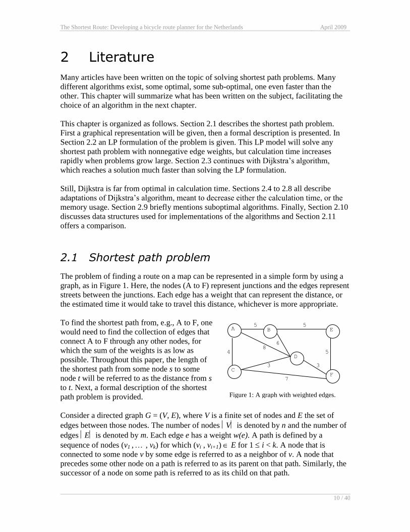
The problem of finding a route on a map can be represented in a simple form by using a

graph, as in Figure 1. Here, the nodes (A to F) represent junctions and the edges represent

streets between the junctions. Each edge has a weight that can represent the distance, or

the estimated time it would take to travel this distance, whichever is more appropriate.

To find the shortest path from, e.g., A to F, one

would need to find the collection of edges that

connect A to F through any other nodes, for

which the sum of the weights is as low as

possible. Throughout this paper, the length of

the shortest path from some node s to some

node t will be referred to as the distance from s

to t. Next, a formal description of the shortest

path problem is provided.

Consider a directed graph G = (V, E), where V is a finite set of nodes and E the set of

edges between those nodes. The number of nodes V is denoted by n and the number of

edges E is denoted by m. Each edge e has a weight w(e). A path is defined by a

sequence of nodes (v1 , , vk) for which (vi , vi+1) E for 1 i < k. A node that is

connected to some node v by some edge is referred to as a neighbor of v. A node that

precedes some other node on a path is referred to as its parent on that path. Similarly, the

successor of a node on some path is referred to as its child on that path.

Figure 1: A graph with weighted edges.


11 / 40

Given a source node s V and a target node t V, the shortest path is defined as the path

(s , , t) that minimizes the sum of the weights of all edges on the path. The length of

the shortest path from s to node v is defined as g(v) and is also referred to as the distance

from s to v.

2.2 LP model

One way to solve a shortest path problem is using the linear programming model

described in [1]. In order to formulate this model, the following variables need to be

defined.

otherwise0

path optimal in the used is edge if1 exe

ii u entering edges ofset the:

ii u leaving edges ofset the:

An LP model can now be defined as shown below.

n

Ee

e ewx )( Minimize

Where

Eex

xx

xx

V\{s,t}i:vxx

e

δe

e

δe

e

δe

e

δe

e

i

δe

e

δe

e

tt

ss

ii

0

1

1

0

The first constraint describes the demand that every node that is not s or t should be left

as many times as it is entered. The second constraint describes that s should be left one

time more than it is entered. The third constraint describes that node t be left one time

less than it is entered. The fourth constraint describes that the decision variables should

be larger than or equal to 0. The model itself ensures all decision variables take either the

value 0 or the value 1, because any other values will lead to a non-optimal solution.

Route planners need to solve shortest path problems of substantial size. For this case, LP

is not the most suitable method to find a solution. No matter how good the model, no


12 / 40

matter how efficient the code, calculation times will grow too large if a problem specific

approach is not used. The following sections describe a number of algorithms that offer a

more efficient way to solve shortest path problems.

2.3 Dijkstra

In [2], Dijkstra describes an algorithm that solves a shortest path problem with

nonnegative edge weights much more efficiently than LP. This algorithm is now known

as Dijkstra’s algorithm and has been documented thoroughly. For each node v, two

properties are stored. The first is the length of the shortest path from s to v found so far,

the second the node preceding v on that path. The algorithm will construct better paths in

an iterative way, improving the solution in each step. Once finished, it will have found

the shortest path from source node s to all other nodes in a graph.

2.3.1 The algorithm

In order to explain the algorithm, the following definitions are needed:

A := the set of nodes v for which a shortest path from s to v has been found (also

known as the closed set).

X := the set of nodes v for which a path from s to v has been found of which it is

uncertain if it is the shortest (also knows as the open set).

ĝ(v) := length of the shortest path from s to v found so far (this can be seen as an

estimate or upper bound for the shortest path from s to v).

ĝ(s) := 0

Initialize the algorithm with:

A =

X = {s}

Repeat the following steps until X equals the empty set.

1. Take node v from X for which )(ˆmin)(ˆ ugvgXu

, remove v from X and add it to A.

2. For each u for which (v, u) E (each neighbor of v)

If u is in A, do nothing.

If u is in X

If ĝ(v) + w(v,u) < ĝ(u), then set ĝ(u) = ĝ(v) + w(v,u) and parent(u) = v.

If u is not in A and not in X, add u to X and set ĝ(u) = ĝ(v) + w(v,u) and parent(u)

= v.

When the algorithm ends, all nodes that can be reached from s will be in A (including t)

and the solution has been found. To save some calculation time, the algorithm can be

stopped once t is moved to A, because at that point the shortest path to t has been found.


13 / 40

2.3.2 Proof of optimality

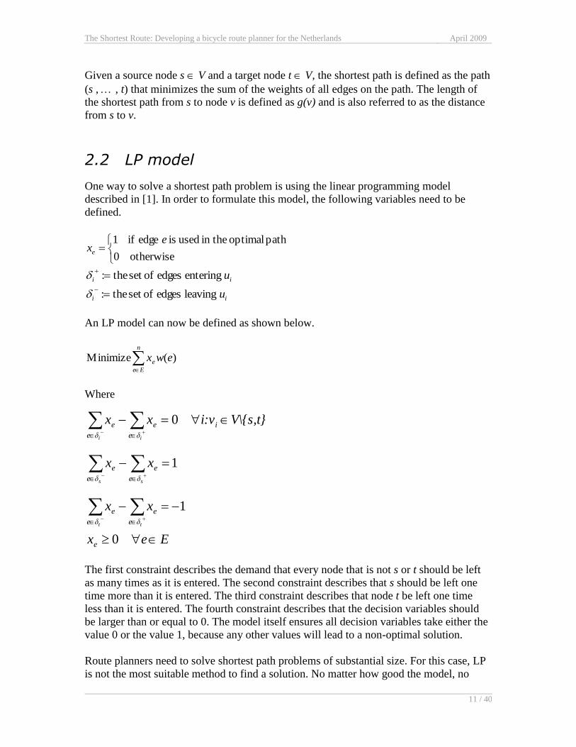
This section will show why Dijkstra always finds an optimal path. See the collection A as

an expanding border around the source node s, where every node inside the border is

closer to s than any node outside the border. A keeps expanding, until it contains the

target node. This principle is illustrated in Figure 2.

Define vk as the node that is added to A in step k. Using induction it is shown that vk is the

node for which the length of the shortest path g(vk) is the shortest of all nodes not in A.

This is trivial for step 1, because s is added with g(s)=0.

Say that this holds up to some step k, then after this step any node not in A will have a

larger distance from s than any node in A. Necessarily, all neighbors of all nodes in A,

will be in X. As a consequence, any node not in A and not in X will have a longer distance

from s than at least one node in X, because you will have to travel through a node in X to

get there. This means the node vk+1 that needs to be added to A in step k+1 will be in X

and will therefore be found by the algorithm.

Because this holds for k = 1, this proves it holds for any k 1, or any step in the

algorithm. Because the shortest path to vk is shorter than to any node outside of A, this

path does not contain any nodes outside of A and therefore the shortest path found so far

is the actual shortest path, or ĝ(vk) = g(vk), making it valid to add it to A. A formal prove

for Dijkstra is provided next.

When a node is added to A, the shortest path is found and the algorithm does not touch

the node again. To prove that the path Dijkstra finds to each node is indeed the shortest

path, we need to prove for each iteration k, there exists no path to vk shorter than ĝ(vk), or

ĝ(vk) = g(vk). For this proof Lemma 1 provided in [3] is used.

A after iteration 1.




A B E

D

C F

5 5

4

3 3

8

7

5

3

Figure 2: Expansion of A in Dijkstra’s algorithm.


14 / 40

Lemma 1

For any optimal path P from s to some node u A, there exists a node v X on P

with ĝ(v) = g(vk).

Proof

If s X, this is trivially true, since ĝ(s) = g(s) = 0. Otherwise, let v* be the node that

was last added to A. Note that this cannot be the same node as v, because v A. Let v

be the successor of v* on P. By definition of ĝ, ĝ(v) ĝ(v*) + w(v*, v). Because v*

A, ĝ(v*) = g(v*) and because P is an optimal path, g(v) = g(v*) + w(v*, v).

Combining these results leads to ĝ(v) g(v), but in general ĝ(v) g(v). From this it

follows that ĝ(v) = g(v).

Lemma 1 shows that for each iteration there is a node vk X where ĝ(vk) = g(vk), as long

as there is a node u A. When this node u does not exist, X equals the empty set and the

algorithm is terminated. This proves that for every node that is added to A the shortest

path has been found, so for every node v A, Dijkstra’s algorithm has found the shortest

path from s to v.

2.4 A*

When traveling to a certain destination, there is usually no point taking a road in the

opposite direction. An algorithm would do well to give priority to roads that travel in the

direction of the destination. That is where Dijkstra falls short. Dijkstra searches the search

space in any direction, as indicated by the fact that the algorithm finds the shortest path

from s to any other node. Clearly, the algorithm does not search in the direction of the

target node.

Hart, Nilsson and Raphael [3] introduce the A* algorithm, that adds a heuristic to

Dijkstra, making it more goal oriented. Instead of evaluating a node v using an estimate

for the shortest path to this node ĝ(v), Hart et al. introduce the following evaluation

function.

)()()( vhvgvf .

The evaluation function f(v) represents the length of the shortest path from the source

node s to the target node t when traveling through node v. The g(v) part is the distance

from s to v and the h(v) part is the distance from v to t. They also introduce an estimate

for the evaluation function:

)(ˆ)(ˆ)(ˆ vhvgvf .

The estimated distance from s to v, ĝ(v), is determined in the same way as in Dijkstra’s

algorithm, the shortest path from s to v found so far. The estimated distance from v to t,

ĥ(v), is determined by using a heuristic. This heuristic can be any function and is often


15 / 40

problem specific; there is no best heuristic. For route planning problems, a heuristic that

is often used is the Euclidean distance from v to t.

The only alteration that A* makes in the algorithm shown in the previous section is that

)(ˆmin)(ˆ ugvgXu

is replaced by )(ˆmin)(ˆ ufvfXu

in step 1.

Next, Hart et al. prove that the A* algorithm finds an optimal solution if

)()(ˆ vhvh for all v.

This is the same as saying the heuristic ĥ(v) should always underestimate the true

distance h(v), or ĥ(v) should give a lower bound on h(v). This is known as an admissible

heuristic.

2.4.1 Proof of optimality

The proof for A* is slightly more complicated than the proof Dijkstra. Russel and Norwig

[4] try to give a feeling for the algorithm by describing the collection A as a contour

around all nodes having f(v)<c for some constant c, much like Dijkstra does for g(v).

With every iteration the value of c is increased and the contour is expanded.

Of course this does not provide a complete proof. Therefore the formal proof from [3] is

given below. First the following corollary to Lemma 1 from the previous section is

needed.

Corollary to lemma 1

Suppose a heuristic h(v) is admissible and A* has not terminated. Then for any

optimal path P from s to t, there exists a node v X with )()(ˆ sfvf .

Proof

By Lemma 1 there exists a node v X on P with ĝ(v) = g(vk). Then:

)ˆ of definition(by )(

)admissible is ˆ (because)()(

1) lemma(by )(ˆ)(

)ˆ of definition(by )(ˆ)(ˆ)(ˆ

fvf

hvhvg

vhvg

fvhvgvf

Suppose A* terminates after finding a non-optimal route to t. Then

)()(ˆ)(ˆ sftgtf . According to the corollary, just before termination, there was

a note v on an optimal path with )()()(ˆ tfsfvf . At this point the algorithm

would have selected v at step 1 instead of t and the algorithm could not have

terminated. This proves that A* cannot terminate after finding a non-optimal route

to t.


16 / 40

2.4.2 Optimally efficient

It should be noted that A* is optimally efficient for any given heuristic function. This

means no other optimal algorithm using the same knowledge is guaranteed to expand

fewer nodes than A*. A short explanation for this is given in [4]: “any algorithm that does

not expand all nodes in the contours between the root and the goal contour runs the risk

of missing the optimal solution”. A formal proof is given in [3].

This observation does not mean there are no ways to get to a solution faster. As shown in

the next sections, by improving the heuristic, or by performing some form of

preprocessing, the calculation time can be decreased significantly.

2.4.3 Memory usage

One downside of both Dijkstra and A* is that when the search space grows large,

memory usage increases rapidly for both methods. A search space may contain millions

of nodes and for each node that is visited by the algorithm one integer ĝ(v) and one

pointer to the preceding node need to be stored in memory. Because of these memory

requirements, methods were developed that can compete with A* in terms of

performance, but use less memory. These algorithms are IDA*, MA* and SMA*.

IDA*

IDA* stands for Iterative Deepening A*. The method is based on Depth First Iterative

Deepening. In each iteration, IDA* sets a threshold for the evaluation function )(ˆ vf . It

then searches one path until the evaluation function for this path exceeds the threshold.

When the threshold is exceeded, the path is backtracked until a node is found with

neighbors that have not been searched yet and the algorithm continues with a path from

this neighbor. An iteration ends when all possible paths up to the threshold have been

searched.

Once an iteration has finished, IDA* sets the threshold for the next iteration to the

minimum of all values found that exceeded the current threshold. This process continues

until the target node has been found.

Although it would seem that IDA* performs a lot of extra calculations by expanding

nodes multiple times, the actual overhead this causes is rather small. The reason behind

this is that the outer layer of the expanded nodes, expanded in the last iteration, contains

by far the most nodes. The fact that other layers are expanded multiple times does not

make much difference. IDA* returns an optimal solution under the same constraints as

A*. A more detailed description of IDA* can be found in [11].

SMA*

The weakness of IDA* is that it effectively throws information away after each iteration.

A method that tries to retain as much information as possible is known as Memory

Bounded A*, or MA* [12]. Russel [13] introduces SMA* that improves MA* by letting

even less information get lost and making the algorithm slightly easier to implement.


17 / 40

SMA* works roughly the same as A*, with the difference that it has a limit on the

number of nodes that are allowed to be stored in memory. Once this limit has been

reached, it will prune a leaf node only when space is needed for a better one. When a

node has to be pruned, it will remove the shallowest node with the highest value of

)(ˆ vf .

In order to prevent unnecessary information loss, information from the successors is

stored in preceding nodes. Once all successors of a node v have been expanded, the value

of )(ˆ vf is replaced by the lowest value of all successors. This information is then

updated for all predecessors of v.

Theorem 4 in [13] says that except for its ability to generate single successors, SMA*

behaves identically to A* when the number of nodes generated by A* does not exceed the

limit. SMA* returns an optimal path when enough memory is available to store the

shallowest optimal solution.

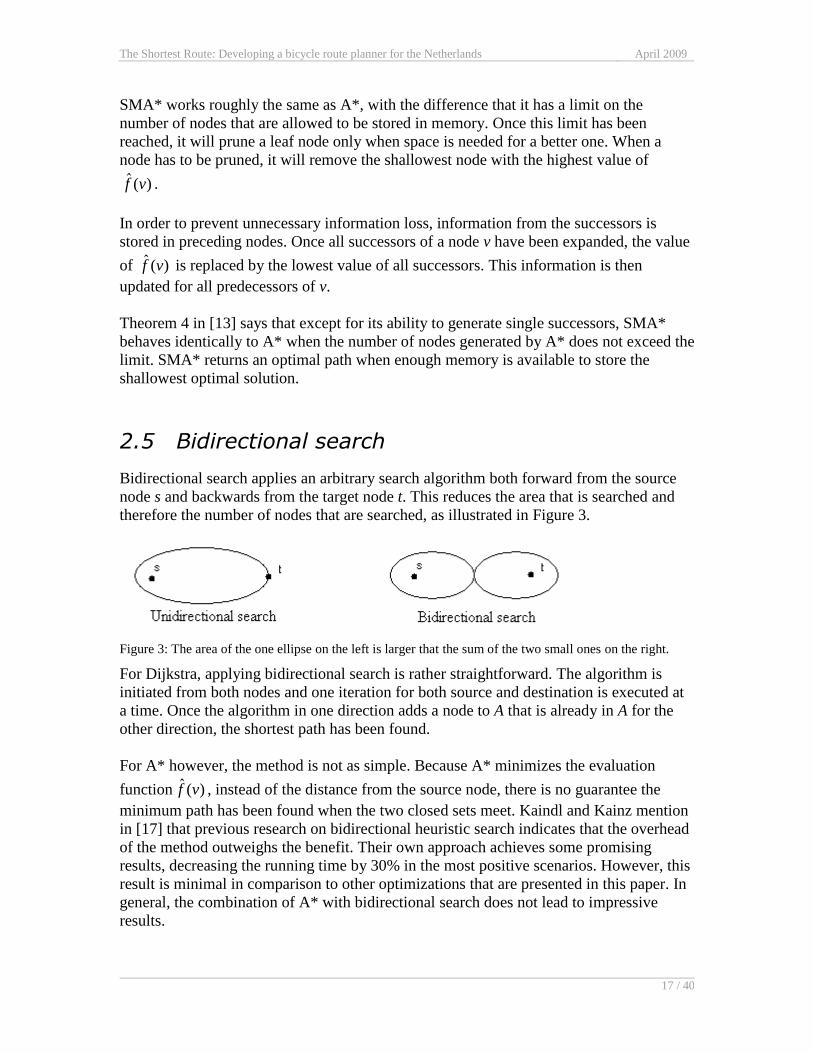
2.5 Bidirectional search

Bidirectional search applies an arbitrary search algorithm both forward from the source

node s and backwards from the target node t. This reduces the area that is searched and

therefore the number of nodes that are searched, as illustrated in Figure 3.

Figure 3: The area of the one ellipse on the left is larger that the sum of the two small ones on the right.

For Dijkstra, applying bidirectional search is rather straightforward. The algorithm is

initiated from both nodes and one iteration for both source and destination is executed at

a time. Once the algorithm in one direction adds a node to A that is already in A for the

other direction, the shortest path has been found.

For A* however, the method is not as simple. Because A* minimizes the evaluation

function )(ˆ vf , instead of the distance from the source node, there is no guarantee the

minimum path has been found when the two closed sets meet. Kaindl and Kainz mention

in [17] that previous research on bidirectional heuristic search indicates that the overhead

of the method outweighs the benefit. Their own approach achieves some promising

results, decreasing the running time by 30% in the most positive scenarios. However, this

result is minimal in comparison to other optimizations that are presented in this paper. In

general, the combination of A* with bidirectional search does not lead to impressive

results.


18 / 40

2.6 Geometric pruning using bounding-boxes

Every road is only useful to get to a number of different places. For any other place, it is

faster to take another road. If this information is known when planning a route, roads that

are not in the shortest path to the destination can easily be ignored. Unfortunately, storing

all this information takes up an enormous amount of memory.

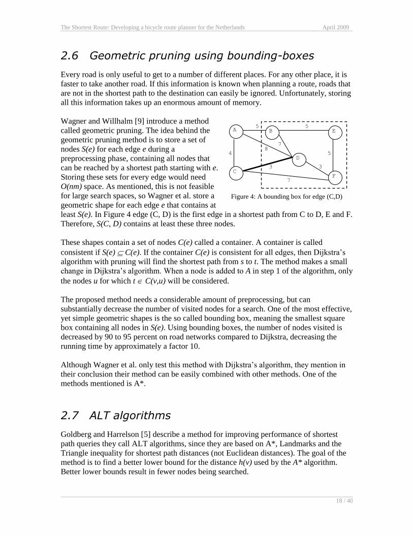
Wagner and Willhalm [9] introduce a method

called geometric pruning. The idea behind the

geometric pruning method is to store a set of

nodes S(e) for each edge e during a

preprocessing phase, containing all nodes that

can be reached by a shortest path starting with e.

Storing these sets for every edge would need

O(nm) space. As mentioned, this is not feasible

for large search spaces, so Wagner et al. store a

geometric shape for each edge e that contains at

least S(e). In Figure 4 edge (C, D) is the first edge in a shortest path from C to D, E and F.

Therefore, S(C, D) contains at least these three nodes.

These shapes contain a set of nodes C(e) called a container. A container is called

consistent if S(e) C(e). If the container C(e) is consistent for all edges, then Dijkstra’s

algorithm with pruning will find the shortest path from s to t. The method makes a small

change in Dijkstra’s algorithm. When a node is added to A in step 1 of the algorithm, only

the nodes u for which t C(v,u) will be considered.

The proposed method needs a considerable amount of preprocessing, but can

substantially decrease the number of visited nodes for a search. One of the most effective,

yet simple geometric shapes is the so called bounding box, meaning the smallest square

box containing all nodes in S(e). Using bounding boxes, the number of nodes visited is

decreased by 90 to 95 percent on road networks compared to Dijkstra, decreasing the

running time by approximately a factor 10.

Although Wagner et al. only test this method with Dijkstra’s algorithm, they mention in

their conclusion their method can be easily combined with other methods. One of the

methods mentioned is A*.

2.7 ALT algorithms

Goldberg and Harrelson [5] describe a method for improving performance of shortest

path queries they call ALT algorithms, since they are based on A*, Landmarks and the

Triangle inequality for shortest path distances (not Euclidean distances). The goal of the

method is to find a better lower bound for the distance h(v) used by the A* algorithm.

Better lower bounds result in fewer nodes being searched.

A B E

D

C F

5 5

4

3 3

8

7

5

7

Figure 4: A bounding box for edge (C,D)


19 / 40

An ALT algorithm selects a number of landmarks during preprocessing. For every node

the distance to and from these landmarks is computed. Consider a landmark L and let

d(u,v) be the distance from any node u to any node v. Then by the triangle inequality,

d(u,L) – d(v,L) d(u,v). Similarly, d(L,v) – d(L,u) d(v,u).

Since d(w,L) and d(L,w) were computed during preprocessing, this fact can then be used

to compute a lower bound for the distance between two nodes. To achieve the tightest

lower bound, the maximum over all landmarks is used. Once the lower bound is found,

this can be used as the heuristic for ĥ(v) in the A* algorithm.

Finding good landmarks is critical for the overall performance of ALT algorithms.

Goldberg et al. describe three ways of selecting landmarks. If k is the number of

landmarks that need to be selected, the simplest method described is selecting k nodes at

random. However, there are better methods.

The second method described is called farthest landmark selection. It is initiated by

picking one random node and picking the node farthest away from it as the first

landmark. Then, for each new landmark that is to be selected, find the node that is

farthest away from the current set of landmarks.

For road maps, having a landmark lying behind the destination tends to give good

bounds. In this case, the method called planar landmark selection is a good choice. Find a

node v near the center of the graph and divide the graph into k pie-slice sectors with v as

their center, so that each slice contains approximately the same number of nodes. Then

for each sector select the node farthest from c as a landmark. To avoid having two

landmarks close to each other, if a landmark in sector A was chosen close to the border of

the next sector B, skip the nodes in B that are close to the border with A.

For the number of landmarks that should be selected, Goldberg et al. suggest a moderate

amount, e.g. 16, as the improvement when choosing more landmarks is relatively small

compared to the extra calculation time. Finally, when calculating a shortest path from s to

t, they suggest taking a small subset of landmarks (e.g. 4) that give the highest lower

bounds on the distance from s to t.

Results show an improved efficiency of a factor 10 to 20 compared to Dijkstra when

using ALT algorithms.

2.8 Multi-level approach

When traveling from one city to another, the largest part of the shortest path will be fixed,

no matter what the exact starting point and destination of the journey is. It is obvious

some paths are part of a large number of different shortest paths. The multi-level

approach tries to take advantage of this fact.


20 / 40

Sanders and Schultes [6], [7] introduce a variant of this method they call highway

hierarchies. Their method creates multiple levels for the original graph during

preprocessing, where each higher level is an abstraction of a lower one. The original

graph is the lowest level. When generating a new level, some nodes and edges may be

removed and some edges may be added.

The multi-level approach tries to find so-called highways in the graph and add these to a

new level. First a neighborhood around each node is determined. Highways consist of

edges that are on a shortest path from some source node s to some target node t and have

their beginning and end outside of both the neighborhoods of s and t and edges that either

leave the neighborhood around s or enter the neighborhood around t, but not both.

Finally some steps are taken to clean up the newly created level. Paths consisting only of

nodes with 2 neighbors are removed completely and replaced by a single edge connecting

the start and end node of the path. Furthermore, all isolated nodes are removed.

Once a new level is created, the steps can be repeated to generate another level. When the

desired number of levels has been created, all nodes in each level are linked to the

corresponding ones in the level below to form the final graph. This step ensures that the

shortest path is found; the algorithm can always take a step down to a more detailed level.

The queries on the final graph are performed by a slightly modified version of the A*

algorithm and were shown to be between 500 and 2,000 times faster than Dijkstra’s

algorithm on real road networks.

2.9 Suboptimal algorithms

Some authors, for instance Botea, Müller, and Schaeffer in [10], have introduced

suboptimal algorithms that lower calculation times significantly, while giving results

within a small margin of the optimal solution. Although this could be interesting, Sanders

and Schultes describe in [8] that shortest path algorithms have improved so much in

terms of speed in the past years, they are actually becoming too fast.

With the latest methods, query times of only a few milliseconds can be achieved, causing

overhead like displaying routes or transmitting them over a network to become the

bottleneck. Considering this argument, it is no longer interesting to accept suboptimal

solutions to decrease query times.

2.10 Priority queue

The data structure behind Dijkstra’s algorithm, or variations of it, can have a significant

effect on the performance. Because Dijkstra and A* will need to find the node in X with

the lowest value for ĝ or ĥ respectively, implementations of Dijkstra, A* or one of their

variations generally use a priority queue, or heap. This type of queue will always have the


21 / 40

value with the highest priority (or in this case the lowest value for ĝ or ĥ) available

without needing to search the whole collection, thereby decreasing processing time.

Dijkstra’s algorithm runs in O(m) time plus the time required to perform the heap

operations. Where Dijkstra’s original implementation, using an array, needed O(n2),

implementations using a Fibonacci heap [14] are able to decrease this to O(m + n log n).

Under certain restrictions double buckets [15], or multi-level buckets [16] can achieve

even greater speed-ups.

A priority queue consists of a set of items, each with its own real-valued key. This type of

queue should support at least the following operations:

Insert(h, x) - Insert item x, with predefined key, into heap h.

Delete min(h) - Find the item with the minimum key in heap h,

delete it from the heap and return it.

Decrease key(h, x, d) - Subtract d from the key of item x in h and replace

its key with this value.

2.10.1 Fibonacci heaps

A Fibonacci heap is designed to not only minimize the time needed for the delete min

operation, but more importantly, the decrease key operation. Because the latter is

generally performed multiple times in each iteration, this approach benefits the running

times for Dijkstra and A*. How this goal is achieved will be explained in this section.

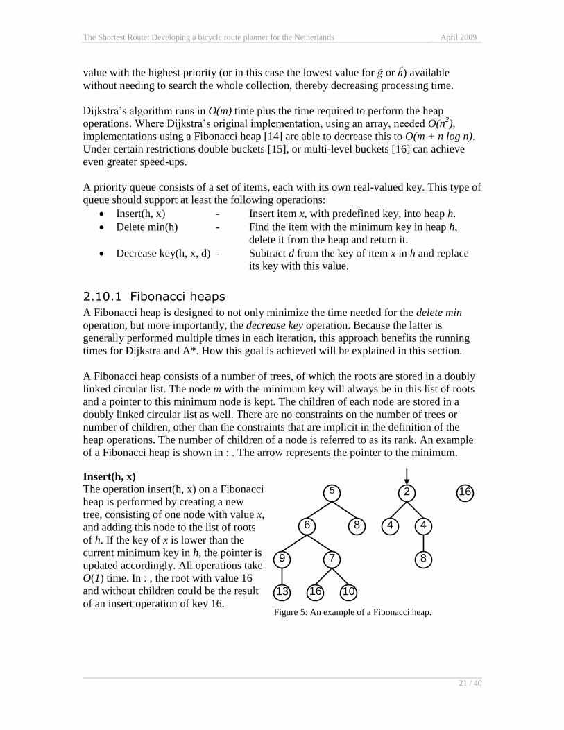
A Fibonacci heap consists of a number of trees, of which the roots are stored in a doubly

linked circular list. The node m with the minimum key will always be in this list of roots

and a pointer to this minimum node is kept. The children of each node are stored in a

doubly linked circular list as well. There are no constraints on the number of trees or

number of children, other than the constraints that are implicit in the definition of the

heap operations. The number of children of a node is referred to as its rank. An example

of a Fibonacci heap is shown in : . The arrow represents the pointer to the minimum.

Insert(h, x)

The operation insert(h, x) on a Fibonacci

heap is performed by creating a new

tree, consisting of one node with value x,

and adding this node to the list of roots

of h. If the key of x is lower than the

current minimum key in h, the pointer is

updated accordingly. All operations take

O(1) time. In : , the root with value 16

and without children could be the result

of an insert operation of key 16. Figure 5: An example of a Fibonacci heap.

5 2 16

6 8 4 4

8 7 9

13 16 10


22 / 40

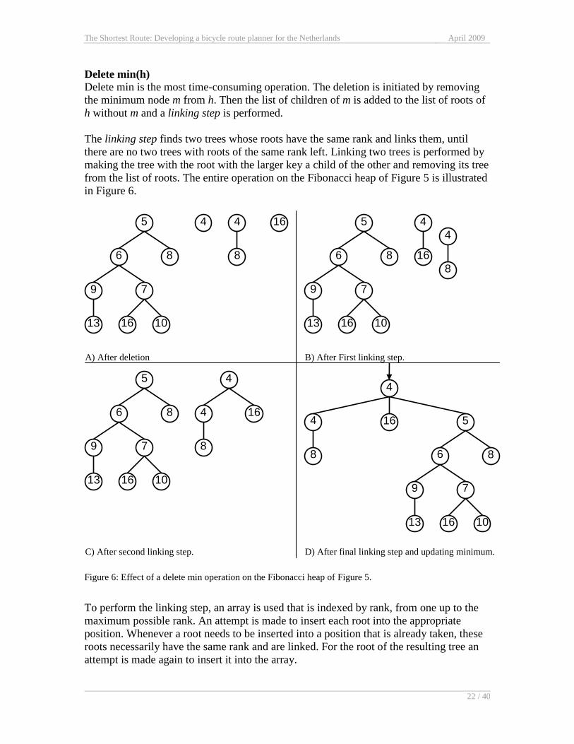
Delete min(h)

Delete min is the most time-consuming operation. The deletion is initiated by removing

the minimum node m from h. Then the list of children of m is added to the list of roots of

h without m and a linking step is performed.

The linking step finds two trees whose roots have the same rank and links them, until

there are no two trees with roots of the same rank left. Linking two trees is performed by

making the tree with the root with the larger key a child of the other and removing its tree

from the list of roots. The entire operation on the Fibonacci heap of Figure 5 is illustrated

in Figure 6.

Figure 6: Effect of a delete min operation on the Fibonacci heap of Figure 5.

To perform the linking step, an array is used that is indexed by rank, from one up to the

maximum possible rank. An attempt is made to insert each root into the appropriate

position. Whenever a root needs to be inserted into a position that is already taken, these

roots necessarily have the same rank and are linked. For the root of the resulting tree an

attempt is made again to insert it into the array.

5 16

6 8

4 4

8

7

16 10

9

13

5

16 6 8

4

7 9

13 16 10

5

16 6 8

4

4

8 7 9

13 16 10

5 16

6 8

4

4

8

7 9

13 16 10

A) After deletion B) After First linking step.

C) After second linking step. D) After final linking step and updating minimum.

4

8


23 / 40

A property of a Fibonacci heap is that a node of rank k has at least Fk+2 φk descendants,

including itself, where Fk is the k-th Fibonacci number and φ = (1 + 5) / 2 is the golden

ratio. Therefore, any root will have a maximum possible rank of logφ n, where n is the

total number of nodes in the heap.

When the linking is finished, the minimum is updated to point to the new minimum in the

root list. The delete min operation takes O(log n), where n is the number of items in the

heap.

Decrease key(h, x, d)

For the decrease key operation, it is assumed that the position of x in h is known. First, d

is subtracted from the key of x. Next, the node k containing x is cut from its parent and

added to the list of roots. This action forms a new tree with k as its root. If k already was a

root, decrease key is performed by simply subtracting d from the key of k.

If the new key of x is smaller than the key of m, the pointer is updated to reflect this. A

decrease key operation takes O(1) time. After each decrease operation, cascading cuts

may have to be performed, as described in the next section.

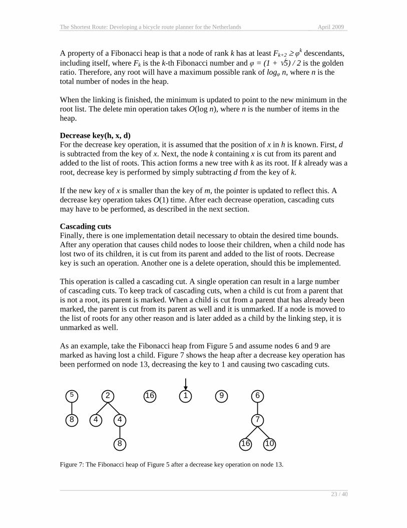
Cascading cuts

Finally, there is one implementation detail necessary to obtain the desired time bounds.

After any operation that causes child nodes to loose their children, when a child node has

lost two of its children, it is cut from its parent and added to the list of roots. Decrease

key is such an operation. Another one is a delete operation, should this be implemented.

This operation is called a cascading cut. A single operation can result in a large number

of cascading cuts. To keep track of cascading cuts, when a child is cut from a parent that

is not a root, its parent is marked. When a child is cut from a parent that has already been

marked, the parent is cut from its parent as well and it is unmarked. If a node is moved to

the list of roots for any other reason and is later added as a child by the linking step, it is

unmarked as well.

As an example, take the Fibonacci heap from Figure 5 and assume nodes 6 and 9 are

marked as having lost a child. Figure 7 shows the heap after a decrease key operation has

been performed on node 13, decreasing the key to 1 and causing two cascading cuts.

Figure 7: The Fibonacci heap of Figure 5 after a decrease key operation on node 13.

5 2 16 6

8 4 4

8

7

9 1

16 10


24 / 40

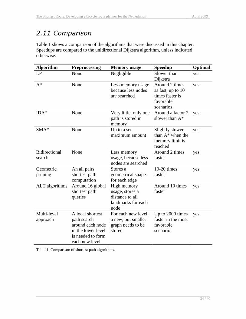
2.11 Comparison

Table 1 shows a comparison of the algorithms that were discussed in this chapter.

Speedups are compared to the unidirectional Dijkstra algorithm, unless indicated

otherwise.

Algorithm Preprocessing Memory usage Speedup Optimal

LP None Negligible Slower than

Dijkstra

yes

A* None Less memory usage

because less nodes

are searched

Around 2 times

as fast, up to 10

times faster is

favorable

scenarios

yes

IDA* None Very little, only one

path is stored in

memory

Around a factor 2

slower than A*

yes

SMA* None Up to a set

maximum amount

Slightly slower

than A* when the

memory limit is

reached

yes

Bidirectional

search

None Less memory

usage, because less

nodes are searched

Around 2 times

faster

yes

Geometric

pruning

An all pairs

shortest path

computation

Stores a

geometrical shape

for each edge

10-20 times

faster

yes

ALT algorithms Around 16 global

shortest path

queries

High memory

usage, stores a

distance to all

landmarks for each

node

Around 10 times

faster

yes

Multi-level

approach

A local shortest

path search

around each node

in the lower level

is needed to form

each new level

For each new level,

a new, but smaller

graph needs to be

stored

Up to 2000 times

faster in the most

favorable

scenario

yes

Table 1: Comparison of shortest path algorithms.


25 / 40

3 Other routing services

There are two main types of existing routing applications: offline, or onboard planners

and online or web planners. Numerous applications of both types exist, this chapter will

only name a few very popular ones and several that are in some way related to this

project.

3.1 TomTom

TomTom is a large international company that offers stand alone navigation devices.

Their devices are among the most popular ones, mainly because of the intuitive user

interface, the speed with which it calculates routes and the accuracy of their data. The

devices can calculate routes by car, by bike or on foot. Unfortunately, their routing

algorithm and data source are not open to the public.

Recently TomTom has released an online version of their route planner as well, however,

this version misses many of the features the stand alone device offers. Among other

things, it lacks an option to plan routes by bike or on foot. Both the online version and the

stand alone version are available in Dutch.

3.2 Google Maps

Google has recently started their own online map and routing service, named Google

Maps. It is a very fast, free service. It is obvious that Google has performed some kind of

preprocessing or caching to make their routing service this fast, but details or their

routing algorithm stay within the company. Google Maps is available in Dutch, but only

offers routes by car and on foot.

3.3 Via Michelin

Via Michelin is an online routing service based on the maps from the well-known

publisher of road maps, Michelin. It is another impressively fast service. The service is

free and seems to have only one purpose, as marking for Michelin. Again, some kind of

preprocessing or caching would be necessary to achieve these calculation times, but this

information is confidential. Via Michelin is available in Dutch and does offer an option to

plan bicycle routes. However, the database lacks information on bicycle paths, so the

results are often inaccurate.


26 / 40

3.4 Routenet.nl

Routenet.nl is a popular Dutch online routing service. The service is not quite as fast as

the previous two, but the calculation times within the Netherlands are still very

acceptable. It is a commercial service that is freely accessible and makes money from

advertisements. Therefore, like TomTom and Google, their routing algorithm and data

are not open to the public. Routenet.nl has recently added the option to plan bicycle

routes, however, like Via Michelin, it lacks information on bicycle paths.

3.5 YourNavigation.org

YourNavigation.org is a demonstration website for the YOURS project. The goal of the

project is to use OpenStreetMap (OSM) data to make a routing website utilizing as much

other (opensource) applications as possible. It uses an opensource routing engine called

Gosmore. The service is not very fast on longer routes and their website mentions that

Gosmore is not designed for generating routes longer than 200km. The routeplanner

offers an option to plan bicycle routes and the does have bicycle paths in their data

source, but it is only available in English.

3.6 OpenRouteService.org

OpenRouteService.org is another online service that uses OSM data. It is a project of the

Geography department of the University of Bonn in Germany. Like YourNavigation.org,

it is a non-commercial service that is free and has no advertising on their website. Apart

from the source code, almost every bit of information on the implementation is available

on the website. The service uses A* and is not as fast on longer routes the commercial

applications. OpenRouteService.org is only available in English, but can plan bicycle

routes. It uses the same data source as YourNavigation.org, so it includes bicycle paths.

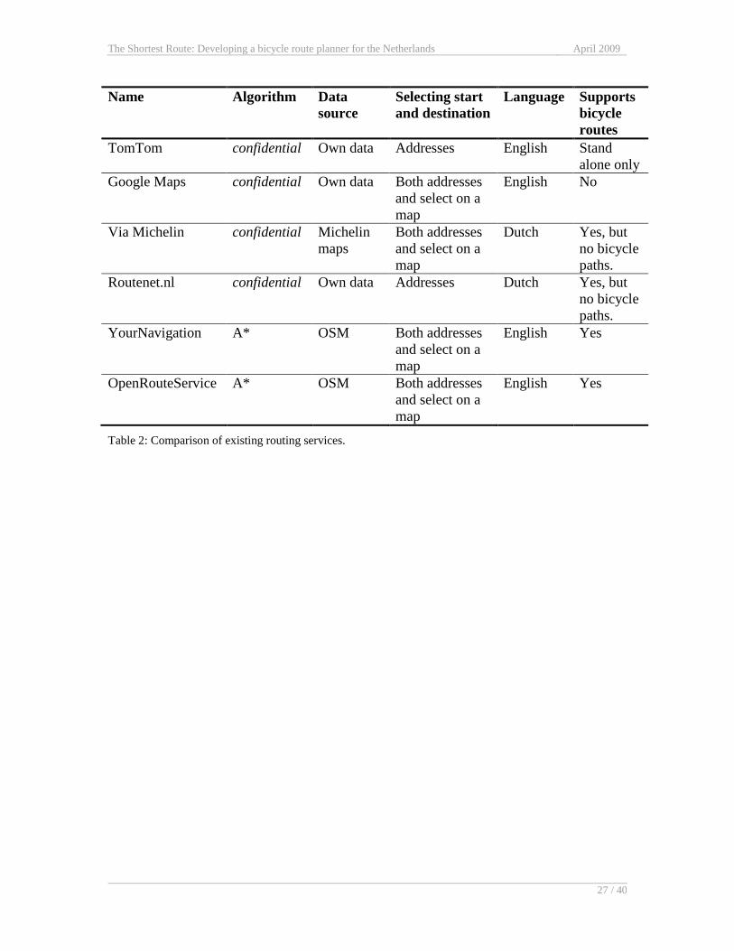
3.7 Comparison

Table 2 shows a comparison of the six routing applications that were discussed in this

section. Unfortunately for the best performing applications the routing algorithms were

confidential. The two that did reveal their routing algorithm both used A*. It is obvious

that non-commercial routing services tend to stick with less complex algorithms, to limit

the time that needs to be invested. Commercial applications have a lot depending on the

performance of their service and can afford to invest more time and money in order to

increase performance.


27 / 40

Name Algorithm Data

source

Selecting start

and destination

Language Supports

bicycle

routes

TomTom confidential Own data Addresses English Stand

alone only

Google Maps confidential Own data Both addresses

and select on a

map

English No

Via Michelin confidential Michelin

maps

Both addresses

and select on a

map

Dutch Yes, but

no bicycle

paths.

Routenet.nl confidential Own data Addresses Dutch Yes, but

no bicycle

paths.

YourNavigation A* OSM Both addresses

and select on a

map

English Yes

OpenRouteService A* OSM Both addresses

and select on a

map

English Yes

Table 2: Comparison of existing routing services.


28 / 40

4 Implementation

As a result of the study performed in Chapter 3, it can be concluded that there still is no

Dutch route planner that offers decent support for planning bicycle routes and covers the

entire Netherlands. Therefore, as part of this project, a bicycle route planner for the

Netherlands will be implemented.

For the implementation, a number of decisions need to be made. First of all the decision

needs to be made what programming language to use. Second, a suitable algorithm needs

to be chosen. Based on the choice of algorithm, a suitable data structure may be needed to

optimize the time for data storage and retrieval. Finally, this data needs to come from

somewhere. A data source with data on all roads in the Netherlands is a requirement for

the success of the project.

This chapter is organized as follows. Sections 4.1 to 4.4 describe these decisions and

other details of the implementation. Section 4.5 shows the resulting application and some

numbers on performance. Section 4.6 presents a validation of the routes the application

finds.

4.1 Programming language

For the choice of programming language, the project implies a number of constraints.

Because the application will likely need a substantial amount of processing time to

calculate a route, the code should be compiled to benefit the speed of the calculations.

Furthermore, to facilitate structured design, maintainability and extensibility of the

application, an object-oriented language should be preferred over a non object-oriented

language.

Taking these constraints into account, several options still remain. The choice was made

to use ASP.NET, specifically C#, based on the availability and previous experience.

4.2 Algorithm

In Chapter 2 several algorithms were described for calculating the shortest route from one

point to another. For the implementation, one algorithm, or a combination of several,

needs to be chosen. The first constraint on this choice is the speed. The algorithm must

find a solution within an acceptable timeframe.

Studies have shown that users start to believe an error has occurred when delays rise

above 10 seconds and quality of service is rated as low for higher delays [18]. An online

service should therefore aim for a response time below 10 seconds. The algorithm should

at least be able to find a solution for any route within 10 seconds, preferably less, since

transmitting results and displaying routes may increase the response time.


29 / 40

The second constraint for the choice of algorithm is complexity. Since there is only a

limited amount of time available for the project, algorithms that are too complex may not

be feasible.

The decision was made to use the A* algorithm with the Euclidean distance as heuristic,

based on two arguments. First of all A* is one of the least complex algorithms, being

only slightly more complex than Dijkstra. Second, methods such as geometrical pruning,

ALT and multi-level approach can be combined with A* with only small adjustments to

the algorithm. The major change for these methods is in the preprocessing phase. As a

result, the application can be easily extended to support any of these methods at a later

time.

The decision to use A* makes the choice for a data structure rather obvious. Because

Fibonacci heaps have been created specifically for Dijkstra and A*, this should be a good

choice.

4.3 Data source

As mentioned before, a data source that can supply accurate data on the complete road

network in the Netherlands is a requirement for the success of the project.

openstreetmap.org offers such a data source.

OpenStreetMap (OSM) is an openly available online world map. Anyone can contribute

GPS data, which is used to form a dataset describing all the roads in the world. The data

is by far not complete, but fortunately Automotive Navigation Data (AND) has donated a

street network of the entire Netherlands. As a result the data is fairly complete for the

Netherlands and a suitable source for the route planner.

The entire street network for the Netherlands (and other countries) can be downloaded as

an XML file. This file contains node tags containing latitude and longitude and way tags

containing the nodes it covers and several tags to indicate the type of road.


30 / 40

A road will be designated as allowing bicycles if at least one of the following tag/value

combinations is included.

Tag Value

highway secondary

tertiary

unclassified

residential

livingstreet

service

track

cycleway

cycleway - any -

cycle

true

yes

1

Table 3: Roads designated as allowing bicycles.

4.4 Other issues

When implementing a route planner, there are a number of issues to take into account.

First of all there are several coordinate systems that can be used to specify a location on

earth. Each system has its benefits and a decision needs to be made on which system to

use. Also selecting a starting point and destination is not as trivial as it seems. Finally, a

way to display the calculated route must be found. This section will describe these issues

and the way they were handled.

4.4.1 Coordinates

The standard method to specify a location on earth is by specifying a longitude and

latitude pair. Latitude is the angle between a point on the Earth's surface and the

equatorial plane. Longitude is the angle east or west of a reference line that was chosen

near Greenwich. The benefit of this sytem is that any location on earth can be pinpointed

exactly. The downside however, is that calculating distances between two locations gets

significantly more complicated. As a result, calculation times grow when distances need

to be calculated often.

Fortunately, these coordinates can be approximated by coordinates in a plane[19], [20].

The exact width of one longitudinal degree on latitude φ can be calculated by

rM)cos(180


31 / 40

where Mr is the earth's average radius, which equals 6,367,449m. The width of one

latitudinal degree can be approximated by

rM180

By calculating longitude and latitude for each node in meters during startup, distances

can be calculated in very little time.

4.4.2 Selecting a starting point and destination

In general, there are two methods of selecting a starting point and destination. Either have

users enter an address, or let them select a location on a map. Unfortunately, both

methods have their own issues.

The dataset from OSM does not specify a town for each way. This makes selecting an

address difficult, because road names can be shared between towns. The second option,

letting the user select a location on a map, creates the difficulty that the selected location

will usually not be exactly on a node.

In the end the second method was implemented. To overcome the problem mentioned,

the closest way to the selected location is determined by calculating the distance to all

nearby ways. The closest node on that way is selected.

4.4.3 Displaying the route

For displaying the route there are again two options. Either use text to describe the route,

or plot the route on a map. Since the map was already available for selecting the starting

point and destination, this was the method that was chosen for the implementation.

4.5 Results

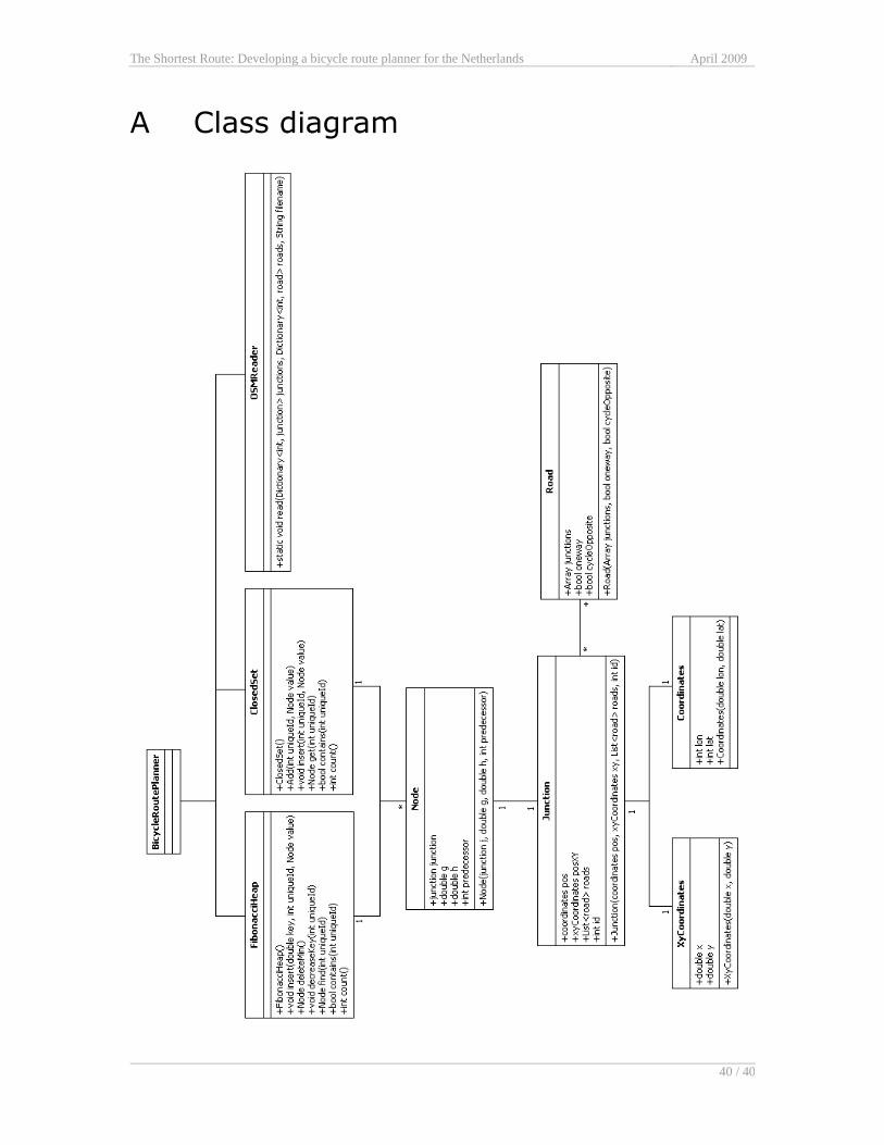
During the course of the project, a bicycle route planner for the Netherlands was

implemented successfully. The application is called Cycle Route Planner. A class

diagram describing the design of the implementation can be found in Appendix A. As

mentioned, a Fibonacci heap is used to implement the open set. For the closed set, a

Dictionary object as present in the C# API was used.

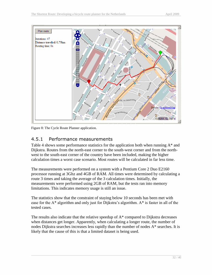
Figure 8 shows the application after a route has been plotted. A starting point can be

selected by left clicking on the map and a destination point by right clicking on the map.

When a user clicks “plan route”, both points are slightly adjusted to match an existing

node and a route between both nodes is calculated and displayed on the map.


32 / 40

Figure 8: The Cycle Route Planner application.

4.5.1 Performance measurements

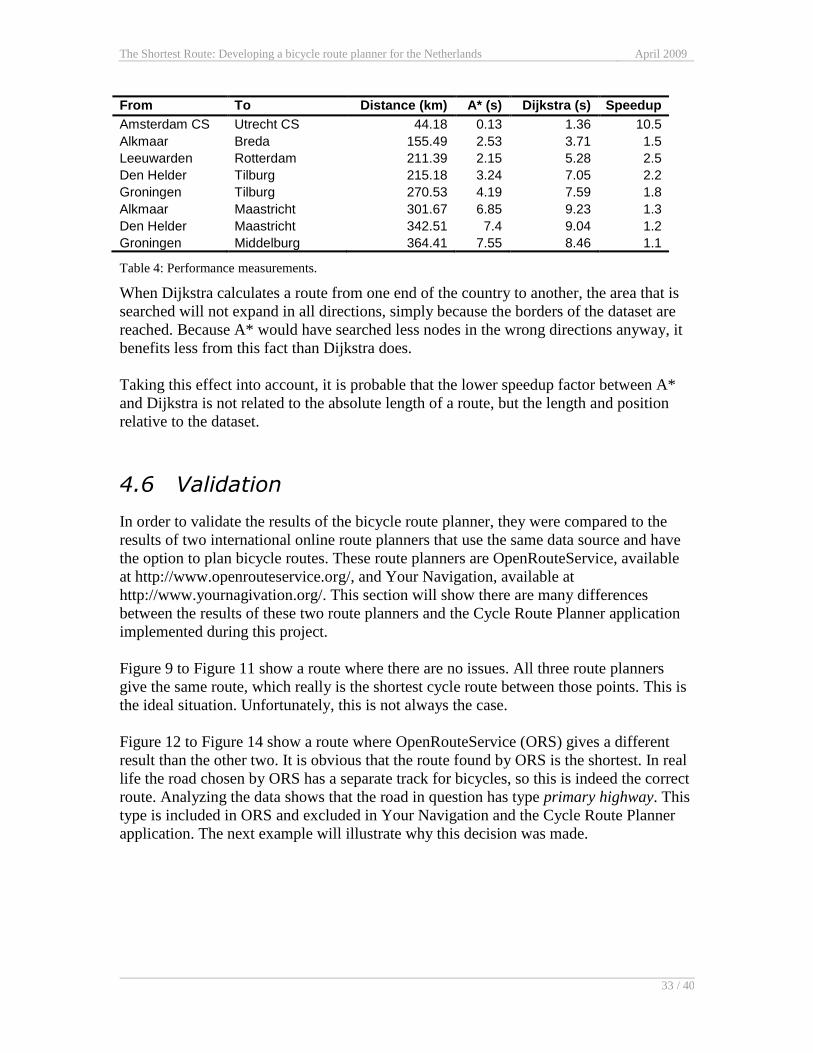
Table 4 shows some performance statistics for the application both when running A* and

Dijkstra. Routes from the north-east corner to the south-west corner and from the north-

west to the south-east corner of the country have been included, making the higher

calculation times a worst case scenario. Most routes will be calculated in far less time.

The measurements were performed on a system with a Pentium Core 2 Duo E2160

processor running at 3Ghz and 4GB of RAM. All times were determined by calculating a

route 3 times and taking the average of the 3 calculation times. Initially, the

measurements were performed using 2GB of RAM, but the tests ran into memory

limitations. This indicates memory usage is still an issue.

The statistics show that the constraint of staying below 10 seconds has been met with

ease for the A* algorithm and only just for Dijkstra’s algorithm. A* is faster in all of the

tested cases.

The results also indicate that the relative speedup of A* compared to Dijkstra decreases

when distances get longer. Apparently, when calculating a longer route, the number of

nodes Dijkstra searches increases less rapidly than the number of nodes A* searches. It is

likely that the cause of this is that a limited dataset is being used.


33 / 40

From To Distance (km) A* (s) Dijkstra (s) Speedup

Amsterdam CS Utrecht CS 44.18 0.13 1.36 10.5

Alkmaar Breda 155.49 2.53 3.71 1.5

Leeuwarden Rotterdam 211.39 2.15 5.28 2.5

Den Helder Tilburg 215.18 3.24 7.05 2.2

Groningen Tilburg 270.53 4.19 7.59 1.8

Alkmaar Maastricht 301.67 6.85 9.23 1.3

Den Helder Maastricht 342.51 7.4 9.04 1.2

Groningen Middelburg 364.41 7.55 8.46 1.1

Table 4: Performance measurements.

When Dijkstra calculates a route from one end of the country to another, the area that is

searched will not expand in all directions, simply because the borders of the dataset are

reached. Because A* would have searched less nodes in the wrong directions anyway, it

benefits less from this fact than Dijkstra does.

Taking this effect into account, it is probable that the lower speedup factor between A*

and Dijkstra is not related to the absolute length of a route, but the length and position

relative to the dataset.

4.6 Validation

In order to validate the results of the bicycle route planner, they were compared to the

results of two international online route planners that use the same data source and have

the option to plan bicycle routes. These route planners are OpenRouteService, available

at http://www.openrouteservice.org/, and Your Navigation, available at

http://www.yournagivation.org/. This section will show there are many differences

between the results of these two route planners and the Cycle Route Planner application

implemented during this project.

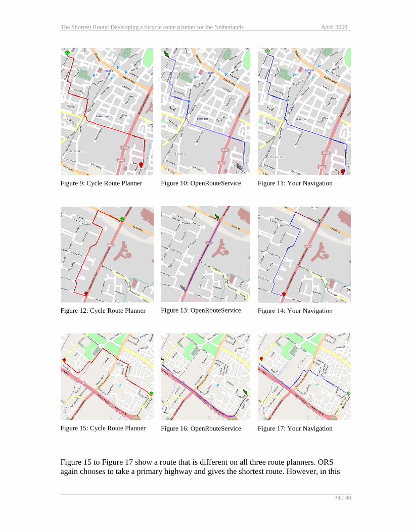
Figure 9 to Figure 11 show a route where there are no issues. All three route planners

give the same route, which really is the shortest cycle route between those points. This is

the ideal situation. Unfortunately, this is not always the case.

Figure 12 to Figure 14 show a route where OpenRouteService (ORS) gives a different

result than the other two. It is obvious that the route found by ORS is the shortest. In real

life the road chosen by ORS has a separate track for bicycles, so this is indeed the correct

route. Analyzing the data shows that the road in question has type primary highway. This

type is included in ORS and excluded in Your Navigation and the Cycle Route Planner

application. The next example will illustrate why this decision was made.


34 / 40

Figure 9: Cycle Route Planner

Figure 10: OpenRouteService

Figure 11: Your Navigation







Figure 15 to Figure 17 show a route that is different on all three route planners. ORS

again chooses to take a primary highway and gives the shortest route. However, in this


35 / 40

case the road does not allow bicycles. As a result, the route given by ORS cannot be

taken by bike, although it should have planned a bicycle route.

The route that Your Navigation gives is still shorter than the one that the Cycle Route

Planner gives. Closer analysis reveals that this route includes a pedestrian path to get to

the destination. This means the Cycle Route Planner is the only planner that actually

gives an admissible route.

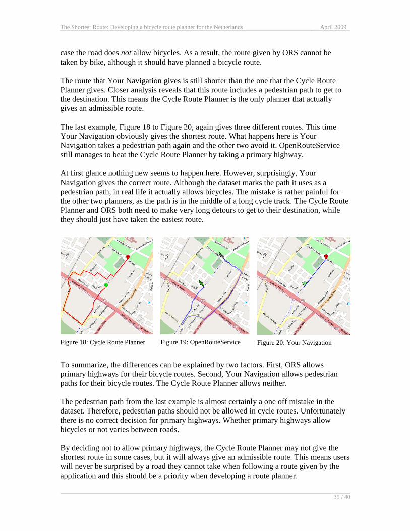
The last example, Figure 18 to Figure 20, again gives three different routes. This time

Your Navigation obviously gives the shortest route. What happens here is Your

Navigation takes a pedestrian path again and the other two avoid it. OpenRouteService

still manages to beat the Cycle Route Planner by taking a primary highway.

At first glance nothing new seems to happen here. However, surprisingly, Your

Navigation gives the correct route. Although the dataset marks the path it uses as a

pedestrian path, in real life it actually allows bicycles. The mistake is rather painful for

the other two planners, as the path is in the middle of a long cycle track. The Cycle Route

Planner and ORS both need to make very long detours to get to their destination, while

they should just have taken the easiest route.




To summarize, the differences can be explained by two factors. First, ORS allows

primary highways for their bicycle routes. Second, Your Navigation allows pedestrian

paths for their bicycle routes. The Cycle Route Planner allows neither.

The pedestrian path from the last example is almost certainly a one off mistake in the

dataset. Therefore, pedestrian paths should not be allowed in cycle routes. Unfortunately

there is no correct decision for primary highways. Whether primary highways allow

bicycles or not varies between roads.

By deciding not to allow primary highways, the Cycle Route Planner may not give the

shortest route in some cases, but it will always give an admissible route. This means users

will never be surprised by a road they cannot take when following a route given by the

application and this should be a priority when developing a route planner.


36 / 40

5 Conclusion & future work

5.1 Conclusion

The most well-known algorithm for solving a shortest path problem is Dijkstra’s

algorithm. However, when implementing an online service, where delays cannot be more

than a few seconds, Dijkstra does not always suffice in terms of speed. Chapter 2

presented several methods to speed it up.

A* and bidirectional search are two methods that only adjust the route calculation

algorithm and lead to small speedups. Geometric pruning, ALT algorithms and the multi-

level approach use preprocessing to analyze the data. Preprocessing may take up to

several hours during startup, but can decrease the query time by impressive amounts.

When using these methods, routes can be found thousands of times faster than when

using Dijkstra. If necessary, most of these methods can even be combined to achieve

even greater speedups. For online route planners, this means that the calculation time can

be decreased to a few milliseconds. With calculation times this small, these no longer

form a bottleneck, but overhead like transmitting the data over a network or displaying

the route will.

Using the knowledge from Chapter 2, a bicycle route planner for the Netherlands was

implemented. The route planner was written in C# and uses A* to calculate the routes,

based on data from openstreetmap.org, which offers a complete road network for the

Netherlands. In order to write the bicycle route planner application, a Fibonacci heap was

implemented in C#. The Fibonacci heap uses general data types and can therefore be

reused in alternate applications.

Performance statistics show that even the longest routes can be calculated within 8

seconds. Quality of service is only rated as low for response times over 10 seconds, so

every route can be calculated with an acceptable QoS. The speedup of A* over Dijkstra is

impressive for shorter routes, but almost negligible for routes that cross the entire

country. Because of inconsistencies in the dataset, the bicycle route planner does not

always give the shortest route. However, it will always give a route that can be taken by

bike. This makes it stand out from the two route planners it was compared with during

validation, where this was not always the case.

5.2 Future work

A relatively easy improvement for the bicycle route planner application would be adding

another method for input and output. Another method for the location input would be to

enter an address as text. This would have to be translated to longitude and latitude by

means of reverse geocoding before it can be mapped to a node. Another method for the


37 / 40

output would be to offer a written description that indicates where to go left or right and

what the streets should be taken.

At the moment, the bicycle route planner supports only Dijkstra’s algorithm and A*,

using a Fibonacci heap for the open set. Implementing additional algorithms and/or data

structures would result in two separate benefits. First, some of the algorithms discussed in

the paper have been shown to decrease processing times substantially. Secondly,

implementing several algorithms and data structures offers the opportunity to compare

their performance.

When several methods are implemented, it should be relatively easy to combine them.

This could lead to even greater speedups. Moreover, comparison of combinations of

algorithms offers another subject of research. Finding the highest performing

combination of algorithms and data structures in order to reach minimal processing times

should offer an interesting challenge.

Finally, it was observed that the speedup of A* compared to Dijkstra grows smaller when

the calculated routes grow larger. As mentioned, this effect is likely the result of the

length and position of the route relative to the dataset. It would be interesting to confirm

this effect for other datasets and see if similar effects can be found when comparing other

methods.


38 / 40

References

1. M. J. de Smith, M. F. Goodchild, and P. A. Longley, “Geospatial Analysis: A

comprehensive guide to principles, techniques, and software tools”, 2nd ed. London:

Troubador, 2007.

2. E. Dijkstra, “A note on two problems in connexion with graphs,” in Numerische

Mathematik, vol. 1. 1959, pp. 269–271.

3. P. E. Hart, N. J. Nilsson and B. Raphael, “A Formal Basis for the Heuristic

Determination of Minimum Cost Paths,” in IEEE Transactions on Systems Science and

Cybernetics SSC4, vol. 2. 1968, pp. 100–107.

4. S. J. Russell and P. Norvig, Artificial Intelligence: A Modern Approach. Englewood

Cliffs, NJ: Prentice Hall, 2003, pp. 55–121.

5. A. V. Goldberg and C. Harrelson, “Computing the shortest path: A search meets

graph theory,” in Proceedings of the Sixteenth Annual ACM-SIAM Symposium on

Discrete Algorithms, 2005, pp. 156-165.

6. P. Sanders and D. Schultes, “Highway hierarchies hasten exact shortest path queries,”

in Proceedings of the 17th European Symposium on Algorithms, 2005, pp. 568–579.

7. P. Sanders and D. Schultes, “Engineering highway hierarchies,” in Proceedings of

the 14th European Symposium on Algorithms, 2006, pp. 804–816.

8. P. Sanders and D. Schultes, “Engineering Fast Route Planning Algorithms,” in 6th

Workshop on Experimental Algorithms, 2007, pp. 23-36.

9. D. Wagner, T. Willhalm, “Geometric Speed-Up Techniques for Finding Shortest

Paths in Large Sparse Graphs,” in Proceedings of the 11th European Symposium on

Algorithms, 2003, pp. 776-787.

10. A. Botea, M. Müller, and J. Schaeffer. Near Optimal Hierarchical Path-finding. In

Journal of Game Development, vol. 1, issue 1, 2004.

11. R. E. Korf, “Depth-first iterative-deepening: an optimal admissible tree search,” in

Artificial Intelligence, vol. 27, 1985, pp. 97-109.

12. P. P. Chakrabarti, S. Ghose, A. Acharya, and S. C. de Sarkar, “Heuristic search in

restricted memory (research note),” in Artificial Intelligence, vol. 41, 1989, pp. 197-222.

13. S. Russell, “Efficient memory-bounded search methods,” in Proceedings of the 10th

European Conference on Artificial intelligence, 1992, pp. 1-5.


39 / 40

14. M. L. Fredman and R. E. Tarjan, “Fibonacci heaps and their uses in improved

network optimization algorithms” in 25th Annual Symposium on Foundations of

Computer Science, 1984, pp. 596-615.

15. B. V. Cherkassky, A. V. Goldberg, and T. Radzik. Shortest Paths Algorithms: Theory

and Experimental Evaluation. In Proc. 5th ACMSIAM Symposium on Discrete

Algorithms, pages 516--525, 1994.

16. A. V. Goldberg and C. Silverstein. Implementations of Dijkstra's Algorithm Based on

Multi-Level Buckets. In Lecture Notes in Economics and Mathematical Systems 450

(Refereed Proceedings), pages 292--327. Springer Verlag, 1997.

17. H. Kaindl and G. Kainz, “Bidirectional heuristic search reconsidered,” in Journal of

Artificial Intelligence Research, vol. 7, 1997, pp. 283-317.

18. A. Bouch, A. Kuchinsky and N. Bhatti. “Quality is in the Eye of the Beholder:

Meeting Users' Requirements for Internet Quality of Service,” in Proceedings of

CHI2000 Conference on Human Factors in Computing Systems, 2000, pp. 297-304.

19. Wikipedia, “Geographic coordinate system,” April 2009. [Online]. Available:

http://en.wikipedia.org/wiki/Geographic_coordinate_system. [Accessed: Apr. 15, 2009].

20. Wikipedia, “Latitude,” April 2009. [Online]. Available:

http://en.wikipedia.org/wiki/Latitude. [Accessed: Apr. 15, 2009].

21. OpenStreetMap, “YOURS”, April 2009 [Online]. Available:

http://wiki.openstreetmap.org/index.php/YOURS. [Accessed: Apr. 28, 2009].


40 / 40

A Class diagram

Documents

The Shortest Route - VU · large amount of route planning software available, ... 2.7 ALT algorithms ... algorithms is given. In Chapter 3 a number of other route planners are discussed