Embed Size (px)
Citation preview

Willeke Veninga
Wageningen University
October 2017
The shadow price of fossil groundwater

ii
MSc thesis Management, Economics and Consumer Studies
Student: Willeke Veninga, 920823-868-120
Supervisors: Dr. ir. A.J. Reinhard
Dr. ir. J.H.M. Peerlings
Examiner: Dr. ir. C. Gardebroek
Date: October 2017

iii
Acknowledgements This thesis was written for Wageningen Economic Research in The Hague, to finish my master
Management, Economics and Governance at Wageningen University. I would like to thank Dr. Stijn
Reinhard of Wageningen Economic Research and Dr. Jack Peerlings of the Agricultural Economics and
Rural Policy Group at Wageningen University, for their advice, quick responses and constructive
feedback during the process of writing this thesis. I would also like to thank Dr. Vincent Linderhof for
his help by the derivation of the translog production function for yield.

iv
Abstract On the basis of a translog production function, a fixed effects panel data model has been estimated to
calculate the shadow prices of non-renewable groundwater for citrus, maize and sugarcane using data
of the twelve largest non-renewable groundwater using countries. Shadow prices of non-renewable
groundwater were positive for citrus and maize during the period 1991-2013, while shadow prices for
sugarcane were negative during the same period. The positive shadow prices indicate that farmers
could increase their yield by adding extra non-renewable groundwater. The negative shadow prices
imply that non-renewable groundwater is used inefficiently since yield is decreased by adding extra
non-renewable groundwater.
v
Contents Acknowledgements ................................................................................................................................. iii
Abstract ................................................................................................................................................... iv
1 Introduction .......................................................................................................................................... 1
2 Theoretical framework ......................................................................................................................... 4
3 Data ...................................................................................................................................................... 6
4 Empirical model .................................................................................................................................... 9
5 Results ................................................................................................................................................ 12
6 Conclusions and discussion ................................................................................................................ 16
References ............................................................................................................................................. 19
Appendix A ............................................................................................................................................ 21
Appendix B ............................................................................................................................................ 26
Appendix C............................................................................................................................................. 29
Appendix D ............................................................................................................................................ 38
Appendix E ............................................................................................................................................. 40
Appendix F ............................................................................................................................................. 42
Appendix G ............................................................................................................................................ 45
Appendix H ............................................................................................................................................ 49

1 Introduction Demand for surface water and groundwater increases worldwide. Drivers are the increasing world
population and increasing standard of living resulting in a higher demand for food (Aeschbach-Hertig
& Gleeson, 2012; Kiani & Abbasi, 2012; Wada et al., 2010; Wada et al., 2014). In most arid and semiarid
areas, agriculture is the largest user of water for crop irrigation during the growing season (Nikouei &
Ward, 2013). In those areas, where surface water availability is limited, additional water originates
mainly from groundwater resources. Use of groundwater is effective for food production in the short
term, but in the long run it is not sustainable (Kiani & Abbasi, 2012). When groundwater extraction
exceeds groundwater recharge, this may result in overexploitation and depletion of aquifers (Wada et
al., 2010; Wada et al., 2014). Figure 1 shows a map of the ratio between the groundwater footprint
and the aquifer area for several
countries across the world. Gleeson et
al. (2012) define the groundwater
footprint as “the area required to
sustain groundwater use and
groundwater use dependent
ecosystem services of a region of
interest”. According to Gleeson et al.
(2012), almost 80% of the global
aquifers can sustain themselves.
Arid areas are dependent on groundwater for food production. For example, the North China Plain is
essential for China’s food provision by providing half of the wheat and one-third of the maize produced
in China (Aeschbach-Hertig & Gleeson, 2012). In those areas groundwater depletion threatens
agricultural production and eventually may lead to a decline in production as water for irrigation
becomes less accessible. Decreasing supply of food crops may lead to a rise in food prices as
groundwater becomes scarcer and water withdrawal costs increase. Figure 1 shows that in particular
poorer parts of the world are vulnerable to groundwater depletion. Trade in agricultural crops may
lead to relatively more indirect water supplies for countries that import groundwater depleting crops
(Dalin et al., 2017). Consequently, depletion of aquifers may affect world food supplies and eventually
increase inequality between consumers in richer and poorer parts of the world.
According to Konikow & Kendy (2005) depletion can be considered both as a reduction in volume of
groundwater and a reduction in quality of fresh groundwater. Quality of residual water in aquifers
Figure 1: Groundwater footprints for six major aquifers (Gleeson et al., 2012)

2
deteriorates by leakage from the land surface; saline or contaminated water from neighbouring
aquifers and sea water intrusion in coastal areas (Aeschbach-Hertig & Gleeson, 2012; Konikow &
Kendy, 2005). Depletion is expected to exaggerate effects from climate change. As more extreme
weather circumstances like droughts and floods will occur, the buffering capacity of groundwater
becomes more important for food production (Taylor et al., 2013). Periods of extreme droughts will
increase demand for irrigation water, while periods of heavy rainfall will change the recharge and
discharge process. Groundwater depletion also contributes to global sea level rise as it reduces
terrestrial water storage capacities and transfers fossil groundwater to the active hydrological cycle
(Wada et al., 2012; Wada et al., 2016).
In many countries, a well-functioning market for water does not exist and the price of groundwater is
not determined by supply and demand. The supply of groundwater is unknown and farmers may not
consider the needs of future generations in their production decisions. Therefore, the price of
groundwater paid by users does not reflect the scarcity. Often, policy with respect to groundwater use
is insufficient or lacking as well. In those countries, groundwater is freely available for land owners who
buy a water pump installation (Famiglietti, 2014). The price paid for groundwater consists of the water
extraction costs and transport costs and does not reflect to the real value of the resource (Ziolkowska,
2015). Therefore, the price of water used for irrigation is below the actual value (Ziolkowska, 2015).
This may result in inefficient water allocation and depletion of aquifers (OECD, 2015; Ziolkowska,
2015). The farmer is assumed to be a price taker and a profit maximiser. The higher the profit, the
higher the chance that the firm will survive. Therefore, production decisions are based on maximising
profit, i.e. the farmer will continue production until the marginal costs are equal to the marginal
revenue. Given the marginal cost of the water input, which is the price the farmer pays for water, the
farmer will add water until he reaches maximum profit. When the price of water is lower than the
actual value, the farmer faces lower marginal costs and he will use more water until he reaches
maximum profit, which may result in depletion.
“Knowledge about the actual value of water as a resource is very limited” (Ziolkowska, 2015). The
actual value of water as a resource, which is unknown, can be approached by the shadow price of
water. Ziolkowska (2015) defines the actual value of water for irrigation as the shadow price of water:
“the ratio between the production net returns and the total amount of water used for irrigating the
respective crops”. Several economic definitions of the shadow price of water are available in literature,
see He et al. (2007). In this paper, we define the shadow price of water as the marginal value of water,
which is the crop value produced by the last m3 of non-renewable groundwater. A relatively low
shadow price indicates that the application of non-renewable groundwater can generate higher crop

3
value for crops with a higher shadow price. Changing production to crops with a higher shadow price
may provide opportunities to reduce non-renewable groundwater use or generate higher crop yields
per m3 of non-renewable groundwater.
This paper aims at determining the shadow price of non-renewable groundwater used to produce
major agricultural crops in the twelve largest non-renewable groundwater consuming countries. The
main research question is: What is the shadow price of non-renewable groundwater for major
agricultural crops in countries that use large quantities of non-renewable groundwater? In order to
answer this question, three sub questions are formulated:
1. How to build a theoretical model for determination of shadow prices?
2. How to solve the empirical model including the available data?
3. What are the inefficiencies in non-renewable groundwater use of countries that
use large quantities of non-renewable groundwater?
Chapter 2 provides the theoretical background. Chapter 3 describes the available data. Chapter 4
contains the empirical model used for estimation in Stata, followed by the results in Chapter 5. The
paper ends with conclusions and a general discussion.

4
2 Theoretical framework This chapter describes how the shadow price of non-renewable groundwater is derived from a
production function. Frank (2010) defines a production function as “the relationship that describes
how inputs are transformed into output”. The shadow price is calculated by multiplying the marginal
product of non-renewable groundwater by the crop output price. The marginal product of non-
renewable groundwater is determined by estimating a production function and taking the partial
derivative with respect to non-renewable groundwater. In this chapter, we describe two types of
production functions that can be used for determining the marginal product. Firstly, we describe the
Cobb-Douglas production function and secondly the trans-log production function, which is a
generalisation of the Cobb-Douglas production function. Appendix A shows the intermediate steps for
deriving the marginal products of all three production functions.
We start with the Cobb-Douglas production function which is most widely used. We consider the inputs
land, labour and capital; three types of water inputs (green, blue and non-renewable groundwater1)
and variable inputs. The Cobb-Douglas production function is represented by the following equation:
𝑌 = 𝛽0 ∙ 𝐴𝛽1 ∙ 𝐿𝛽2 ∙ 𝐾𝛽3 ∙ 𝐺𝑊𝛽4 ∙ 𝐵𝑊𝛽5 ∙ 𝑁𝑅𝐺𝑊𝛽6 ∙ 𝑋𝛽7
(1)
where Y= crop production, A= area, L= labour, K= capital, GW= green water, BW= blue water, NRGW=
non-renewable groundwater, X= variable inputs and β’s are model coefficients. This equation can be
rewritten into log form for estimation purposes:
𝑙𝑛𝑌 = 𝑙𝑛𝛽0 + ∑ 𝛽𝑖
𝑛
𝑖=1
𝑙𝑛𝐼𝑖
(2)
where 𝐼𝑖= inputs (area, labour, capital, green water, blue water, non-renewable water and variable
inputs). The marginal product of non-renewable groundwater (𝑀𝑃𝑁𝑅𝐺𝑊) is derived by taking the
partial derivative of crop production with respect to non-renewable groundwater:
𝑀𝑃𝑁𝑅𝐺𝑊 =𝜕𝑌
𝜕𝑁𝑅𝐺𝑊= 𝛽6 ∙
𝑌
𝑁𝑅𝐺𝑊
(3)
Multiplying the marginal product by the crop output price gives the shadow price:
𝑃𝑠ℎ𝑎𝑑𝑜𝑤 = 𝑝𝑜𝑢𝑡𝑝𝑢𝑡 ∙ 𝑀𝑃𝑁𝑅𝐺𝑊
(4)
1 The types of water inputs are green water (evapotranspiration flows), blue water (withdrawal from rivers, surface water and renewable groundwater) and non-renewable groundwater (Oki & Kanae, 2006).

5
where Pshadow= shadow price and poutput= crop output price.
The Cobb-Douglas production function assumes that all inputs are substitutes and that the elasticity
of substitution between inputs is equal to one. This implies that our model assumes that green, blue
and groundwater are substitutes. However, the hydrological model (which provides the data for the
water inputs) states that green, blue and non-renewable groundwater are applied in sequence (Wada
et al., 2014). If we include this statement in our model, all types of water should be aggregated into
one water input. In that case, the marginal product of water is the marginal product of the last applied
water source. This reflects a situation where on the margin only one out of three water sources will
adjust due to a change in one of the other variables. Still, the farmer may have a choice in application
of blue water or non-renewable groundwater and the amounts of both. We prefer to analyse the
different effects of green water (the amount of green water applied is not influenced by the farmer)
and water applied by the farmer on the crop yield. Therefore, we decide to include green water (GW)
as a separate input and blue water together with non-renewable groundwater as a separate input (WI)
in the production functions. The marginal product of the water input is equal to the marginal product
of non-renewable groundwater, if non-renewable groundwater is applied.
Estimating a trans-log production function may be more appropriate since this functional form allows
for more flexibility and does not impose that all inputs are substitutes and that the substitution
elasticity equals 1, in contrast to the Cobb-Douglas production function. An F-test can be performed
to decide if the trans-log production function is more appropriate than the Cobb-Douglas production
function. A trans-log production function is represented by the following equation:
𝑙𝑛𝑌 = 𝑙𝑛𝛽0 + ∑ 𝛽𝑖
𝑛
𝑖=1
𝑙𝑛𝐼𝑖 +1
2∑ 𝛽𝑖𝑖
𝑛
𝑖=1
𝑙𝑛𝐼𝑖2 + ∑ ∑ 𝛽𝑖𝑗
𝑛
𝑗
𝑛
𝑖 <
𝑙𝑛𝐼𝑖𝑙𝑛𝐼𝑗
(5)
where Y= crop production; 𝐼𝑖 and 𝐼𝑗 are inputs (area, labour, capital, GW, WI and variable inputs) and
𝛽𝑖, 𝛽𝑖𝑖 and 𝛽𝑖𝑗 are model coefficients. The marginal product of the water input is derived by taking the
partial derivative of crop production with respect to the water input:
𝑀𝑃𝑊𝐼 =𝜕𝑙𝑛𝑌
𝜕𝑙𝑛𝑊𝐼∙
𝑌
𝑊𝐼= (𝛾0 + 𝛾1𝑙𝑛𝑊𝐼 + 𝛾2𝑙𝑛𝐴 + 𝛾3𝑙𝑛𝐿 + 𝛾4𝑙𝑛𝐾 + 𝛾5𝑙𝑛𝑊𝐼) ∙
𝑌
𝑊𝐼
(6)
where 𝛾0 = 𝛽5, 𝛾1 = 𝛽65, 𝛾2 = 𝛽15, 𝛾3 = 𝛽25, 𝛾4 = 𝛽35 and 𝛾5 = 𝛽45.
6
3 Data This chapter describes the data used for our empirical research. We provide a general description of
our data, the correlation coefficients and the outcomes of panel unit root tests. For our research, we
selected the twelve largest non-renewable groundwater using countries, which are: China, Egypt,
India, Iran, Italy, Mexico, Pakistan, Saudi Arabia, South Africa, Spain, Turkey and USA (Bierkens et al.,
2016). The focus is on maize, sugarcane and citrus, since we want to estimate production functions for
high and low water consumption crops. Sugarcane and maize have relatively high crop water needs,
while citrus has relatively low crop water needs compared to the standard grass (FAO, 1986).
Moreover, these crops are produced by a large part of the twelve countries, see Appendix B for an
overview of the most important crops produced by each country.
For each crop, we have production (tonnes), total area (ha) and producer prices (USD/tonne) retrieved
from the FAO database. Data for production and area are available from 1961-2014 and data for
producer prices are available from 1991-2014 (FAO, 2016a, 2016b). Water consumption rates (km3)
are retrieved from the global hydrological model (PCRGLOB-WB) developed by Wada et al. (2014). This
model provides data for three water sources: actual evapotranspiration (green water); surface water
and renewable groundwater (blue water) and non-renewable groundwater used by plants, for the
period 1971-2010. Data on the amount of capital, labour and variable inputs per crop are not available.
Therefore, we use agricultural value added per worker (USD) as proxy for capital, employment in
agriculture (1000 persons) as proxy for labour and fertiliser (kg/ ha) as proxy for variable inputs. Data
for fertiliser are retrieved from the Worldbank database and available for all twelve countries from
2003-2014. Data for agricultural value added per worker and employment in agriculture are also
retrieved from the Worldbank database for the same period, but there are many missing observations.
For the period 2003-2010, all observations for agricultural value added per worker and employment in
agriculture are available for Italy, South Africa, Spain and the USA.
Table 1 contains the means, standard deviations and minimum and maximum values of the available
data for citrus, maize and sugarcane, produced by the countries in our sample. India does not produce
any significant amount of citrus, therefore data for India are not included in the estimation of citrus.
Italy, Saudi Arabia, Spain and Turkey do not produce (any significant amount of) sugarcane (see
Appendix B). Therefore, data of these countries cannot be included for this crop. Large differences
exist between the minimum and maximum values of production, hectares grown and water application
for all three commodities (Table 1). Considering the means of water application, sugarcane uses most
non-renewable groundwater compared to citrus and maize, while maize uses most green water

7
compared to the other crops. Considering each crop separately, citrus and sugarcane use most blue
water and maize uses most green water.
Table 1: Summary statistics for the variables in the production functions of citrus, maize and sugarcane: production (tonnes), area (ha), GW (km3), BW (km3) and NRGW (km3)
Variable Mean Std. Dev. Min. Value Max. Value
Citrus Production 3633975 4164741 7800 2.65E+07
Area 243068 322227 1350 2196000
GW 494.89 890.11 0.17 4004.66
BW 746.74 1079.33 6.30 5018.64
NRGW 166.71 187.76 6.81 734.73
Maize Production 3.01E+07 6.39E+07 606 3.33E+08
Area 5974784 9123658 392 3.50E+07
GW 11514.90 22572.77 0.02 99322.94
BW 8469.98 13698.01 1.10 97237.98
NRGW 528.81 757.48 1.87 4856.50
Sugarcane Production 5.31E+07 7.11E+07 578000 3.56E+08
Area 852016 1108850 4536 5150000
GW 2632.36 3556.06 15.55 15215.94
BW 4636.64 6126.94 52.95 25762.30
NRGW 1290.72 2152.67 10.25 10390.09
Table 2 gives an overview of the correlation coefficients of the variables for citrus, maize and
sugarcane. A more extensive overview of all correlation coefficients, including the quadratic terms and
cross terms of the variables, is provided in Appendix D. Overall, the correlation coefficients between
the water inputs are rather high (Table 4). Blue water and green water are highly correlated for all
three crops. For sugarcane, blue water and green water are also highly correlated with non-renewable
groundwater. This may lead to multicollinearity and biased estimators when the production functions
are estimated. A possible explanation for the high correlations coefficients is a common trend, due to
e.g. technological progress, in our data. Therefore, we add a time variable into our empirical model.
Using two water inputs instead of three water inputs may also reduce the risk of multicollinearity.

8
Table 2: Correlation coefficients for variables in the production functions of citrus, maize and sugarcane
Production Area GW BW NRGW
Citrus Production 1.0000
Area 0.7705 1.0000
GW 0.5346 0.8271 1.0000
BW 0.5289 0.8264 0.9907 1.0000
NRGW 0.2208 0.2712 0.2092 0.2668 1.0000
Maize Production 1.0000
Area 0.9294 1.0000
GW 0.9591 0.9190 1.0000
BW 0.8207 0.8530 0.8784 1.0000
NRGW 0.2832 0.5172 0.2740 0.4350 1.0000
Sugarcane Production 1.0000
Area 0.9861 1.0000
GW 0.9607 0.9607 1.0000
BW 0.9756 0.9863 0.9857 1.0000
NRGW 0.8387 0.8774 0.7515 0.8424 1.0000
For stationarity testing we used the Levin–Lin–Chu test, which tests for unit roots in panel datasets.
The null hypothesis states that each time series contains a unit root and the alternative hypothesis
states that each time series is stationary (Baltagi, 2008). In a stationary process, the mean, variance
and covariance of the error term are constant over time. A non-stationary variable cannot be used for
predicting the future based on observations in the past. Details about the Levin–Lin–Chu test are
available in the Stata manual (Stata, 2015). Table 3 provides an overview of the panel variables of
citrus, maize and sugarcane. In this table, yes means that the data are stationary and no means that
the data are nonstationary. Using the natural logarithm of the data solves the non-stationarity problem
to a large extent. Still, the production data of maize and the blue water and non-renewable
groundwater data of sugarcane are nonstationary (Table 3). This problem is largely solved by panel
data estimation since this estimation method uses the first differences of the data. Appendix C contains
all panel graphs and panel unit root tests for the variables of citrus, maize and sugarcane.
Table 3: Results of the panel stationarity tests for the variables in the production functions of citrus, maize and sugarcane, where yes means stationary and no means nonstationary
* Yes/No: Depends on the addition of a trend in the Levin-Lin-Chu test, see Appendix C for the details.
Citrus Maize Sugarcane
Original Ln Original Ln Original Ln Production No Yes No No Yes/No* Yes Yield No Yes No Yes Yes Yes GW No Yes Yes Yes Yes/No* Yes BW No Yes No Yes No No NRGW No Yes Yes/No* Yes Yes/No* No

9
4 Empirical model Several alternative model specifications and estimation methods exist for estimating the production
functions. We decide to perform our estimations with a trans-log specification, since this functional
form allows for more flexibility than the Cobb-Douglas production function (see Chapter 2). We start
with estimating the production function per country, including the proxies for the input variables, using
OLS. Data are available for the following four countries: Italy, South Africa, Spain and the USA for the
period 2003-2010. However, due to the limited number of observations per country, the available
degrees of freedom are insufficient and it is not possible to calculate unbiased and efficient estimators.
Therefore, we estimate the following production function for the four countries together (i.e. cross-
section):
ln 𝑌𝑖 = 𝛽0 + 𝛽1𝑙𝑛𝐴𝑖 + 𝛽2𝑙𝑛𝐸𝑚𝑝𝑖 + 𝛽3𝑙𝑛𝐴𝑉𝐴𝑖 + 𝛽4𝑙𝑛𝐺𝑊𝑖 + 𝛽5𝑙𝑛𝑊𝐼𝑖 + 𝛽6𝑙𝑛𝐹𝑒𝑟𝑖 + 0.5𝛽7𝑙𝑛𝐴𝑖2
+ 0.5𝛽8𝑙𝑛𝐸𝑚𝑝𝑖2 + 0.5𝛽9𝑙𝑛𝐴𝑉𝐴𝑖
2 + 0.5𝛽10𝑙𝑛𝐺𝑊𝑖2 + 0.5𝛽11𝑙𝑛𝑊𝐼𝑖
2
+ 0.5𝛽12𝑙𝑛𝐹𝑒𝑟𝑖2 + 𝛽13𝑙𝑛𝐴𝑖 ∙ 𝑙𝑛𝐸𝑚𝑝𝑖 + 𝛽14𝑙𝑛𝐴𝑖 ∙ 𝑙𝑛𝐴𝑉𝐴𝑖 + 𝛽15𝑙𝑛𝐴𝑖 ∙ 𝑙𝑛𝐺𝑊𝑖
+ 𝛽16𝑙𝑛𝐴𝑖 ∙ 𝑙𝑛𝑊𝐼𝑖 + 𝛽17𝑙𝑛𝐴𝑖 ∙ 𝑙𝑛𝐹𝑒𝑟𝑖 + 𝛽18𝑙𝑛𝐸𝑚𝑝𝑖 ∙ 𝑙𝑛𝐴𝑉𝐴𝑖 + 𝛽19𝑙𝑛𝐸𝑚𝑝𝑖 ∙ 𝑙𝑛𝐺𝑊𝑖
+ 𝛽20𝑙𝑛𝐸𝑚𝑝𝑖 ∙ 𝑙𝑛𝑊𝐼𝑖 + 𝛽21𝑙𝑛𝐸𝑚𝑝𝑖 ∙ 𝑙𝑛𝐹𝑒𝑟𝑖 + 𝛽22𝑙𝑛𝐴𝑉𝐴𝑖 ∙ 𝑙𝑛𝐺𝑊𝑖 + 𝛽23𝑙𝑛𝐴𝑉𝐴𝑖
∙ 𝑙𝑛𝑊𝐼𝑖 + 𝛽24𝑙𝑛𝐴𝑉𝐴𝑖 ∙ 𝑙𝑛𝐹𝑒𝑟𝑖 + 𝛽25𝑙𝑛𝐺𝑊𝑖 ∙ 𝑙𝑛𝑊𝐼𝑖 + 𝛽26𝑙𝑛𝐺𝑊𝑖 ∙ 𝑙𝑛𝐹𝑒𝑟𝑖 + 𝛽27𝑙𝑛𝑊𝐼𝑖
∙ 𝑙𝑛𝐹𝑒𝑟𝑖 + 𝛽28𝑙𝑛t + μ𝑖
(7)
where 𝑌= production, 𝐴= area, 𝐸𝑚𝑝= employment in agriculture, 𝐴𝑉𝐴= agricultural value added per
worker, 𝐺𝑊= green water, 𝑊𝐼= aggregate water input (blue water and non-renewable groundwater),
𝐹𝑒𝑟= fertiliser, 𝑖= number of observations= 1, …, 32 and μ𝑖= random error term. The estimation results
are available in Appendix E. However, Italy and Spain do not produce sugarcane. Consequently, the
production function for sugarcane cannot be estimated and estimation results for sugarcane are not
available in Appendix E.
The estimation results may be improved by using the data of all countries (i.e. cross-section), which
ensures enough degrees of freedom. Unfortunately, data of proxy variables for some inputs are not
available for all countries, so these data cannot be included. Therefore, the following equation is
estimated:

10
𝑙𝑛𝑌𝑖𝑡 = 𝛽0 + 𝛽1𝑙𝑛𝐴𝑖𝑡 + 𝛽2𝑙𝑛𝐺𝑊𝑖𝑡 + 𝛽3𝑙𝑛𝑊𝐼𝑖𝑡 + 0.5𝛽4(𝑙𝑛𝐴𝑖𝑡)2 + 0.5𝛽5(𝑙𝑛𝐺𝑊𝑖𝑡)2
+ 0.5𝛽6(𝑙𝑛𝑊𝐼𝑖𝑡)2 + 𝛽7𝑙𝑛𝐴𝑖𝑡 ∙ 𝑙𝑛𝐺𝑊𝑖𝑡 + 𝛽8𝑙𝑛𝐴𝑖𝑡 ∙ 𝑙𝑛𝑊𝐼𝑖𝑡 + 𝛽9𝑙𝑛𝐺𝑊𝑖𝑡 ∙ 𝑙𝑛𝑊𝐼𝑖𝑡
+ 𝛽10𝑙𝑛𝑡𝑖𝑡 + ∑ 𝛽10+𝑖
12
𝑖=1
𝐷𝑢𝑚𝑖 + 𝜀𝑖𝑡
(8)
where 𝑖= country= 1,…,122, 𝑡= year= 1,...,40 and 𝐷𝑢𝑚= country dummy variable. In this regression, all
observations are taken together and we assume that the observations are not related over time. We
include a dummy for each country to distinguish country specific effects. The production function of
maize includes twelve country dummies. The productions functions of citrus and sugarcane include
eleven and eight country dummies respectively. The USA is used as reference country. Appendix F
contains the regression results for OLS estimation including the country dummy variables.
An alternative for a cross-section model with country dummies is panel data estimation. Panel data
analysis allows for repeated observations over the same units during a number of periods (Verbeek,
2012). Both a fixed effects model and random effects model can be estimated. A fixed effects model
contains a unit specific intercept and is represented by the following equation:
𝑙𝑛𝑌𝑖𝑡 = 𝛼𝑖 + ∑ 𝛽𝑖
𝑛
𝑖=1
𝑙𝑛𝐼𝑖𝑡 +1
2∑ 𝛽𝑖𝑖
𝑛
𝑖=1
𝑙𝑛𝐼𝑖𝑡2 + ∑ ∑ 𝛽𝑖𝑗
𝑛
𝑗
𝑛
𝑖 <
𝑙𝑛𝐼𝑖𝑡𝑙𝑛𝐼𝑗𝑡 + ε𝑖𝑡
(9)
where 𝐼= inputs (𝐴, 𝐺𝑊 and 𝑊𝐼), 𝛼𝑖= unit specific intercept, ε𝑖𝑡= residual term, 𝑖 and 𝑗= country=
1,…,12 and 𝑡= year= 1,...,40. Estimation of fixed effects is based on within variation (variation over time
for a given unit). The random effects model combines within and between variation (variation between
units) and is represented by the following equation:
𝑙𝑛𝑌𝑖𝑡 = μ + ∑ 𝛽𝑖
𝑛
𝑖=1
𝑙𝑛𝐼𝑖𝑡 +1
2∑ 𝛽𝑖𝑖
𝑛
𝑖=1
𝑙𝑛𝐼𝑖𝑡2 + ∑ ∑ 𝛽𝑖𝑗
𝑛
𝑗
𝑛
𝑖
𝑙𝑛𝐼𝑖𝑡𝑙𝑛𝐼𝑗𝑡 + 𝛼𝑖 + ε𝑖𝑡
(10)
where μ= intercept, 𝛼𝑖= individual specific residual (not varying over time) and ε𝑖𝑡 = common residual
term. See Appendix A for derivation of the panel data production funtions for yield.
A fixed effects model can be considered as rather similar to the model with country dummies since the
country specific effects are estimated by the unit specific intercepts. However, a fixed effects model
has less parameters to be estimated and less degrees of freedom compared to the model with country
2 In equation (7) 𝑖 means number of observations; in equation (8) - (11) 𝑖 means number of countries.
11
dummy variables (Appendix F and Appendix G). Advantages of panel data estimation are the modelling
of time and unit-specific effects; the potential omitted variable bias is smaller; separation of within
and between variation; smaller effect of multicollinearity and more efficient estimates (Baltagi, 2008;
Verbeek, 2012). Our estimations are likely to suffer from omitted variable bias, since no data are
available for the labour, capital and variable inputs for the entire period. The water inputs are highly
correlated which may enlarge the risk of multicollinearity. Therefore, panel data estimation is most
appropriate for estimation of the production functions with our data. First-difference transformations
in fixed effects estimation have the cost of losing one year of data for each variable and losing all time-
invariant variables. Consequently, there is a trade-off between the loss of data and more efficient
estimates.
Usually, total production is used as dependent variable in production functions. However, large
differences in total production exist between the countries, see Appendix C for the graphs of total
citrus, maize and sugarcane production per country. Therefore, it may be appropriate to use yield
(production per ha) instead of total production as dependent variable, which enables comparison
between countries. Using yield as dependent variable implies that the interpretation of the parameters
of the production function is slightly different:
𝑙𝑛 (𝑌𝑖𝑡
𝐴𝑖𝑡) = 𝛾0 + 𝛾1𝑙𝑛𝐴𝑖𝑡 + 𝛾2 (
𝑙𝑛𝐺𝑊𝑖𝑡
𝑙𝑛𝐴𝑖𝑡) + 𝛾3 (
𝑙𝑛𝑊𝐼𝑖𝑡
𝑙𝑛𝐴𝑖𝑡) + 𝛾4𝑙𝑛2𝐴𝑖𝑡 + 𝛾5 (
𝑙𝑛𝐺𝑊𝑖𝑡
𝑙𝑛𝐴𝑖𝑡) 𝑙𝑛𝐴𝑖𝑡
+ 𝛾6 (𝑙𝑛𝑊𝐼𝑖𝑡
𝑙𝑛𝐴𝑖𝑡) 𝑙𝑛𝐴𝑖𝑡 + 𝛾7 (
𝑙𝑛𝐺𝑊𝑖𝑡
𝑙𝑛𝐴𝑖𝑡)
2
+ 𝛾8 (𝑙𝑛𝑊𝐼𝑖𝑡
𝑙𝑛𝐴𝑖𝑡)
2
+ 𝛾9 (𝑙𝑛𝐺𝑊𝑖𝑡
𝑙𝑛𝐴𝑖𝑡) (
𝑙𝑛𝑊𝐼𝑖𝑡
𝑙𝑛𝐴𝑖𝑡)
+ 𝛾10𝑙𝑛𝑡𝑖𝑡 + ε𝑖𝑡
(11)
where 𝛾0 = 𝛽0, 𝛾1 = (𝛽1 + 𝛽2 + 𝛽3 − 1), 𝛾2 = 𝛽2, 𝛾3 = 𝛽3, 𝛾4 = (0.5𝛽4 + 𝛽7 + 𝛽8 + 0.5𝛽5 + 𝛽9 +
0.5𝛽6), 𝛾5 = (𝛽7 + 𝛽5 + 𝛽9), 𝛾6 = (𝛽8 + 𝛽6 + 𝛽9), 𝛾7 = 0.5𝛽5, 𝛾8 = 0.5𝛽6 and 𝛾9 = 𝛽9.
Appendix A shows the derivation of the trans-log production function for yield and a description of the
marginal products. The regression results for both production and yield estimation are available in
Appendix G.

12
5 Results Three estimation methods, described in the previous chapter, could be used for calculation of the
shadow prices: OLS estimation including proxy variables (model 1); OLS estimation including country
dummy variables (model 2) and panel data estimation (model 3). First, the input elasticities are
calculated to see if the estimated production function behaves like a translog production function
(output is monotonically increasing in all inputs and diminishing marginal productivity) (Boisvert,
1982). The following formula is used for calculating the input elasticities (Boisvert, 1982):
𝑒𝑖 =𝜕 ln 𝑦
𝜕 ln 𝑥𝑖= 𝛼𝑖 + ∑ 𝛽𝑖𝑗
𝑛
𝑗=1
ln 𝑥𝑗 (𝑖 = 1, … , 𝑛)
(12)
where 𝑦= production, 𝑥𝑗= input j and 𝛼𝑖 and 𝛽𝑖𝑗 are unknown parameters. Table 4 shows the input
elasticities for the green water variable and the water input variable in the production functions of
citrus, maize and sugarcane. The calculations are performed for the OLS estimation methods including
proxy variables and dummy variables.
For model 1, the input elasticities are calculated for
citrus and maize since no estimation results are
available for sugarcane. For both crops, the green
water and water inputs are relatively inelastic
(absolute value of the input elasticity is smaller than
1), which implies that the production is not very
sensitive to a change in water input. Both input
elasticities of citrus are positive, in accordance to the
assumption of the translog production function.
However, the water input elasticity of maize is
negative, which is not in accordance with the assumption of the translog production function.
Moreover, none of the estimated parameters is significant (see Appendix E) and just four countries
could be included to estimate the production functions of citrus and maize. Therefore, we conclude
that the estimation results of model 1 are insufficient to be used for the calculation of the shadow
prices.
For model 2, the water input elasticities are relatively inelastic. This is reasonable for citrus and maize
since these crops are relatively low water consuming crops. However, for sugarcane we would expect
a higher water input elasticity since this crop is a high water consuming crop (and in particular blue
Variable OLS with proxies
OLS with dummies
Citrus GW 0.69 -1.03
WI 0.87 0.37
Maize GW 0.23 -1.18
WI -0.22 0.36
Sugarcane GW n.a. 0.60
WI n.a. -0.33
Table 4: Input elasticities of the green water variable and the water input variable in the production functions of citrus, maize and sugarcane using OLS estimation

13
water). The water input elasticities of citrus and maize are positive, in contrast to the water input
elasticity of sugarcane. The negative water input elasticity for sugarcane is not what we expected
according to the assumptions of the translog production function but reasonable since sugarcane is
produced in wet areas with water abundance. The green water inputs for citrus and maize are rather
elastic (absolute value of the input elasticity is greater than 1), implying that citrus and maize
production are relatively sensitive to a change in green water input. However, the negative elasticities
are not in accordance with the assumptions of the translog production function. Considering the
advantages of model 3 compared to model 2 (described in Chapter 4) and the negative input elasticities
in model 2, we decide not to use the estimation results of model 2 for the calculation of the shadow
prices. Table 5 shows the input elasticities for model 3. When production is estimated, the input
elasticity of area is larger than 1 for all three crops. Indicating that there are increasing returns to scale
(an increase in area results in a higher increase in output). For citrus and maize, all input elasticities
are positive which corresponds with the assumption of the translog production function. The water
input elasticities for sugarcane are negative3 (as in model 2). Possible reasons are an excess of water
supply to sugarcane or insufficient data.
Table 4: Elasticities of the input variables in the production functions of citrus, maize and sugarcane using fixed effects panel estimation
Citrus Maize Sugarcane
Production Yield Production Yield Production Yield
Area 1.15 0.04 1.22 0.09 1.21 0.01
GW 0.06 0.02 0.49 0.50 0.49 0.44
WI 0.37 0.27 0.33 0.32 -0.29 -0.33
Hausman’s specification test is performed to test if the fixed effects model or random effects model is
appropriate. In the Hausman test two estimators are compared: the fixed effects estimator is
consistent under the null and alternative hypothesis and the random effects estimator is consistent
(and efficient) under the null hypothesis only (Verbeek, 2012). Details about the Hausman test are
available in the Stata manual (Stata, 2015). Hausman’s test indicated that the fixed effects model was
most appropriate for all three crops. The estimation results for the fixed effects regression are offered
in Table 6. Both production and yield are estimated for each crop. Table 6 shows that for most variables
there is considerable variation. Moreover, many estimates are non-significant. The three reported R2
measures are defined as the squared correlation coefficients between the actual and fitted values
(Verbeek, 2012). They explain the within variation, between variation and overall variation (which is
3 When a Cobb-Douglas production function for sugarcane yield is estimated, the elasticities of area, green water and water input are positive: 0.06, 0.32 and 0.39 respectively, see Appendix I for the estimates.
14
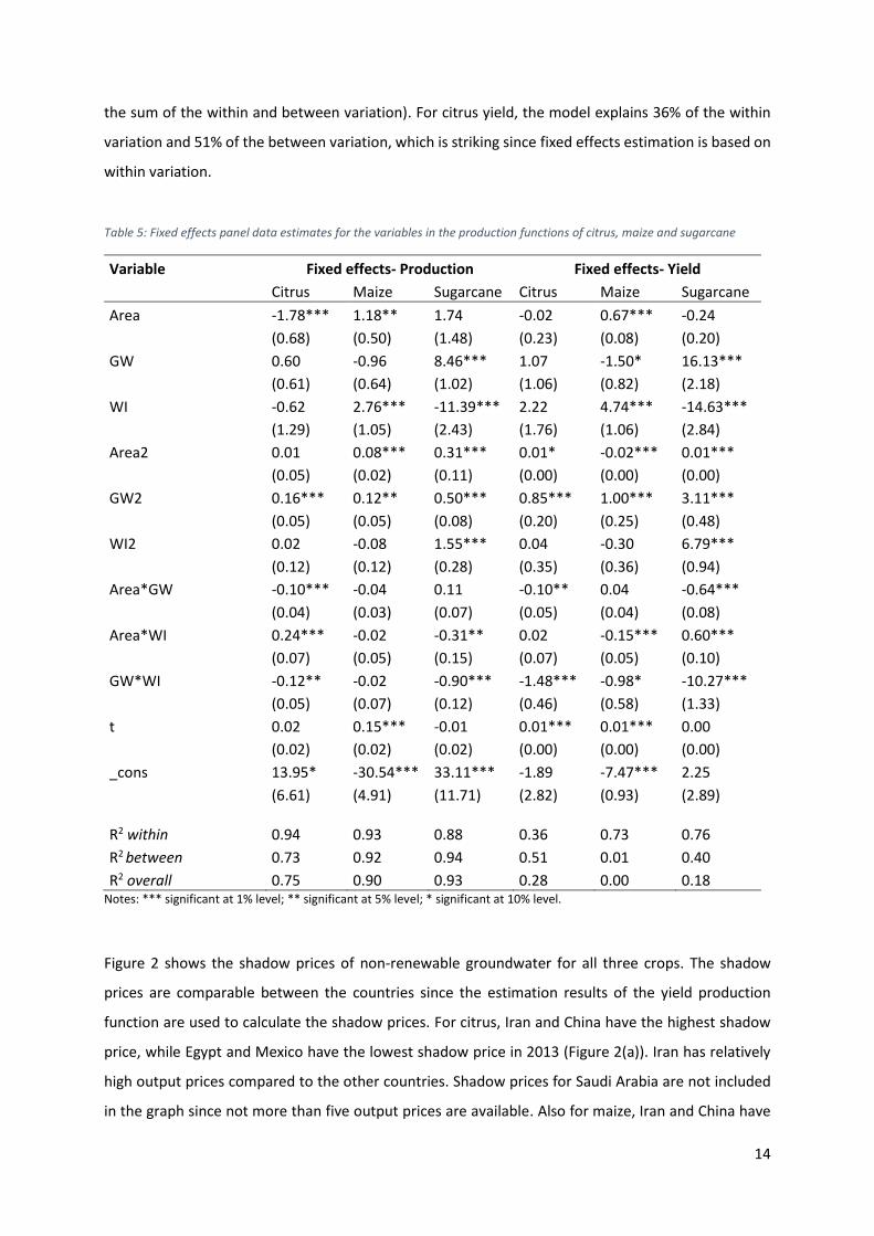
the sum of the within and between variation). For citrus yield, the model explains 36% of the within
variation and 51% of the between variation, which is striking since fixed effects estimation is based on
within variation.
Table 5: Fixed effects panel data estimates for the variables in the production functions of citrus, maize and sugarcane
Variable Fixed effects- Production Fixed effects- Yield
Citrus Maize Sugarcane Citrus Maize Sugarcane
Area -1.78*** 1.18** 1.74 -0.02 0.67*** -0.24
(0.68) (0.50) (1.48) (0.23) (0.08) (0.20)
GW 0.60 -0.96 8.46*** 1.07 -1.50* 16.13***
(0.61) (0.64) (1.02) (1.06) (0.82) (2.18)
WI -0.62 2.76*** -11.39*** 2.22 4.74*** -14.63***
(1.29) (1.05) (2.43) (1.76) (1.06) (2.84)
Area2 0.01 0.08*** 0.31*** 0.01* -0.02*** 0.01***
(0.05) (0.02) (0.11) (0.00) (0.00) (0.00)
GW2 0.16*** 0.12** 0.50*** 0.85*** 1.00*** 3.11***
(0.05) (0.05) (0.08) (0.20) (0.25) (0.48)
WI2 0.02 -0.08 1.55*** 0.04 -0.30 6.79***
(0.12) (0.12) (0.28) (0.35) (0.36) (0.94)
Area*GW -0.10*** -0.04 0.11 -0.10** 0.04 -0.64***
(0.04) (0.03) (0.07) (0.05) (0.04) (0.08)
Area*WI 0.24*** -0.02 -0.31** 0.02 -0.15*** 0.60***
(0.07) (0.05) (0.15) (0.07) (0.05) (0.10)
GW*WI -0.12** -0.02 -0.90*** -1.48*** -0.98* -10.27***
(0.05) (0.07) (0.12) (0.46) (0.58) (1.33)
t 0.02 0.15*** -0.01 0.01*** 0.01*** 0.00
(0.02) (0.02) (0.02) (0.00) (0.00) (0.00)
_cons 13.95* -30.54*** 33.11*** -1.89 -7.47*** 2.25
(6.61) (4.91) (11.71) (2.82) (0.93) (2.89) R2 within 0.94 0.93 0.88 0.36 0.73 0.76
R2 between 0.73 0.92 0.94 0.51 0.01 0.40
R2 overall 0.75 0.90 0.93 0.28 0.00 0.18 Notes: *** significant at 1% level; ** significant at 5% level; * significant at 10% level.
Figure 2 shows the shadow prices of non-renewable groundwater for all three crops. The shadow
prices are comparable between the countries since the estimation results of the yield production
function are used to calculate the shadow prices. For citrus, Iran and China have the highest shadow
price, while Egypt and Mexico have the lowest shadow price in 2013 (Figure 2(a)). Iran has relatively
high output prices compared to the other countries. Shadow prices for Saudi Arabia are not included
in the graph since not more than five output prices are available. Also for maize, Iran and China have

15
the highest shadow prices in 2013. South Africa and the USA have the lowest shadow prices, indicating
that a m3 of non-renewable groundwater generates the lowest crop value in those countries in 2013.
Overall, the graph shows an upward trend in shadow prices between 1991-2013 (Figure 2(b)). The
shadow prices for sugarcane are negative (Figure 2(c)). This is not what we expected and could be
caused by adding to much groundwater to sugarcane or an inappropriate model for sugarcane yield
estimation. Therefore, the results for sugarcane should be handled with care.
0
0,2
0,4
0,6
0,8
1
1 9 9 1 1 9 9 3 1 9 9 5 1 9 9 7 1 9 9 9 2 0 0 1 2 0 0 3 2 0 0 5 2 0 0 7 2 0 0 9 2 0 1 1 2 0 1 3
SHA
DO
WP
RIC
E ($
/M3
)
YEAR
SHADOWPRICES FOR CITRUS (A)
Iran Italy Mexico Pakistan
South Africa Spain Turkey USA
China Egypt
0
0,1
0,2
0,3
0,4
0,5
0,6
1 9 9 1 1 9 9 3 1 9 9 5 1 9 9 7 2 0 0 0 2 0 0 2 2 0 0 4 2 0 0 6 2 0 0 8 2 0 1 0 2 0 1 2 2 0 1 4SHA
DO
WP
RIC
E ($
/M3
)
YEAR
SHADOWPRICES FOR MAIZE (B)
India Iran Italy Mexico
Pakistan South Africa Spain Turkey
USA China Egypt
-0,8
-0,6
-0,4
-0,2
0
1 9 9 1 1 9 9 3 1 9 9 5 1 9 9 7 1 9 9 9 2 0 0 1 2 0 0 3 2 0 0 5 2 0 0 7 2 0 0 9 2 0 1 1 2 0 1 3
SHA
DO
WP
RIC
E ($
/M3
)
YEAR
SHADOWPRICES FOR SUGARCANE (C)
India Mexico Pakistan South Africa
Spain USA China Egypt
Figure 2: Shadow prices of non-renewable groundwater for citrus (a), maize (b) and sugarcane (c) between 1991 and 2014.
16
6 Conclusions and discussion This chapter provides the answers on the research questions which are presented in Chapter 1. In
addition, we deliver a general reflection on the model we used and show how the results are related
to previous studies. On the basis of a translog production function, a fixed effects panel data model
has been estimated to calculate the shadow prices of non-renewable groundwater for citrus, maize
and sugarcane by including data of the twelve largest non-renewable groundwater using countries.
Crop yield is used as dependent variable which enables comparison between the countries. Area, green
water and water input (blue water and non-renewable groundwater) are the independent variables in
our model. All independent variables are converted to inputs per hectare. Taking the partial derivative
of crop yield with respect to the water input gives the marginal product of non-renewable
groundwater. Multiplying the marginal product by the crop output price gives the shadow price. A
fixed effects panel data model was most appropriate since this model results in more efficient
estimates compared to other estimation methods. We tested if a fixed effects model would be more
appropriate than a random effects model, which was not the case.
We found positive shadow prices for non-renewable groundwater applied to citrus and maize during
the period 1991-2013, indicating that farmers could increase their yield by adding extra non-renewable
groundwater. In 2013, shadow prices for citrus ranged between 0.81 USD/m3 and 0.15 USD/m3 and
for maize between 0.53 USD/m3 and 0.19 USD/m3. For sugarcane, we found negative shadow prices,
ranging between -0.10 USD/m3 and -0.62 USD/m3 in 2013. A negative shadow price implies that for
each m3 non-renewable groundwater added yield is decreased, i.e. farmers could increase their profits
when they decrease the non-renewable water input for sugarcane. Probably, risk plays an important
role in the farmer’s water application decision. Sugarcane is a high water consumption crop. Farmers
may apply an excess of water since the price for water is low and they are avoiding the risk of lower
yield due to a deficiency in water application. We recommend to calculate shadow prices for more
crops. Results can be used to determine the optimal crop mix to be produced in a certain region,
dependent on the aim of reducing non-renewable groundwater use or maximising crop yield per m3
of non-renewable groundwater. In the first case, farmers should produce a crop (mix) which generates
the same profit but uses less non-renewable groundwater (i.e. crops that generate a higher value per
added m3 of non-renewable groundwater). In the latter case, farmers produce the crop with the
highest shadow price for non-renewable groundwater.
Our model might suffer from omitted variable(s) since no data were available for labour, capital and
variable inputs for each country. These variables are usually included into a production function. In

17
panel data estimation, the potential omitted variable bias is smaller compared to ordinary least
squares estimation (Baltagi, 2008). We decided to estimate a translog production function however a
Cobb-Douglas and quadratic production can be estimated as well. Our research obtained one marginal
product for farmers in all countries together. The research may be further improved by estimating the
production function for each country separately which results in a specific marginal product for each
country. The production level for maximum profit is reached when the value of the marginal product
is equal to zero. Comparison of marginal products between countries provides an inside in the
production efficiency of crops per country. Some countries can produce a certain crop more efficiently
and use groundwater more efficiently.
Groundwater depletion can be considered as an external cost. Other people (probably in the future)
may face higher costs because of a shortage of non-renewable groundwater, while they are not
involved in the decisions about groundwater use. These external costs are not included in the farmer’s
decision making. Therefore, government regulation should prevent groundwater depletion and
encourage farmers to produce a crop mix that reduces non-renewable groundwater use. In order to
reduce inefficient groundwater use, production of crops with a negative shadow price, like sugarcane,
should be banned in regions with a risk of groundwater depletion. Regulations should be developed
for the amount of non-renewable groundwater used for irrigation since a well-functioning market for
water does not exist. In environmental policy two main types of economic instruments exist: price-
based measures (e.g. taxes or charges) and rights-based measures (e.g. tradeable permits) (Carter,
2001). De Fraiture & Perry (2002) show that irrigation water demand is inelastic at low prices. The
response of water demand to increased water charges is therefore low until a certain threshold (water
price is equal to productive value), beyond that threshold water demand becomes elastic. Only a
considerable increase in water prices can encourage farmers to use less water for irrigation (De
Fraiture & Perry, 2002). Governments can maintain a ban on certain crops rather easy at relatively low
costs, since it is visible which crop is produced. However, if the government sets charges or permits for
groundwater use, this system should be monitored which involves additional costs. In some of the
largest non-renewable groundwater using countries this system may also be vulnerable to corruption.
According to Kumar (2006), water use can be broadly divided into three categories: agricultural,
industrial and domestic. In our research, we calculated shadow prices for agricultural water use. Liu
and Chen (2008) calculated shadow prices for industrial water (all water used in the industrial sector)
and productive water (all water used in agriculture, industry, construction and service sectors) in nine
river basins in China in 1999. They found that shadow prices were higher for industrial water than for
productive water for each river basin. Shadow prices for industrial water range between 0.18 RMB/ton

18
(≈0.03 USD/m3) and 5.13 RMB/ton (≈0.77 USD/m3), while shadow prices for productive water range
between 0.02 RMB/ton (≈0.003 USD/m3) and 2.34 RMB/ton (≈0.35 USD/m3). Their explanation for the
lower shadow price for productive water is that productive water mainly consists of agricultural water,
which is free or very low priced in China. The shadow prices we found for China in 1999 (citrus 0.13
USD/m3 and maize 0.16 USD/m3) fit well within the range of shadow prices for productive water found
by Liu and Chen (2008).
Kumar (2006) investigated the water demand of 92 manufacturing firms in India between 1996/97 and
1998/99. He found an average shadow price of 7.21 INR/m3 (≈0.11 USD/m3). This shadow price is
comparable to the shadow price we found for maize in India (0.12 USD/m3 for 1996, 1997 and 1998),
implying that the average value produced by the last m3 of water was not higher for the industrial
sector than for maize production. Kumar (2006)found that the price elasticity for water in the industrial
sector in India is high (-1.11 on average), so in this sector water charges may be more effective than in
the agricultural sector. Ziolkowska (2015) analysed the shadow prices of irrigation water in three High
Plain states in the USA: Texas, Kansas and Nebraska. The estimated values of shadow prices for maize
were 0.07 USD/m3 (Texas Northern High Plain), 0.004 USD/m3 (Texas Southern High Plain), 0.06
USD/m3 (Kansas) and 0.02 USD/m3 (Nebraska) in 2010. These values are substantially lower than the
shadow price of 0.22 USD/m3 which we found for maize in the USA in 2010. Shadow prices may differ
per region, and therefore our model results may be further improved by estimating a production
function per region rather than per country.

19
References Aeschbach-Hertig, W., & Gleeson, T. (2012). Regional strategies for the accelerating global problem of
groundwater depletion. Nature Geoscience, 5(12), 853-861.
Baltagi, B. (2008). Econometric analysis of panel data: John Wiley & Sons.
Bierkens, M. F. P., Reinhard, S., Bruijn, J. d., & Wada, Y. (2016). The shadow price of fossil groundwater.
Paper presented at the AGU, San Fansisco.
Boisvert, R. N. (1982). The Translog Production Function: Its Properties, Its Several Interpretations and
Estimation Problems. Cornell University, Department of Applied Economics and Management.
Carter, N. (2001). The politics of the environment: Ideas, activism, policy: Cambridge University Press.
Dalin, C., Wada, Y., Kastner, T., & Puma, M. J. (2017). Groundwater depletion embedded in
international food trade. Nature, 543(7647), 700-704.
De Fraiture, C., & Perry, C. (2002). Why is irrigation water demand inelastic at low price ranges. Paper
presented at the Conference on Irrigation Water Policies: Micro and Macro Considerations.
Famiglietti, J. (2014). The global groundwater crisis. Nature Climate Change, 4(11), 945-948.
FAO. (1986). Irrigation Water Management: Irrigation Water Needs. Rome, Italy.
FAO. (2016a). Crop Statistics: Production. Retrieved from: http://www.fao.org/faostat/en/#data/QC
FAO. (2016b). Price Statistics: Producer Prices- Annual. Retrieved from:
http://www.fao.org/faostat/en/#data/PP
Frank, R. H. (2010). Microeconomics and Behavior (8th ed.). New York: The McGraw-Hill Companies,
Inc.
Gleeson, T., Wada, Y., Bierkens, M. F., & van Beek, L. P. (2012). Water balance of global aquifers
revealed by groundwater footprint. Nature, 488(7410), 197-200.
He, J., Chen, X., Shi, Y., & Li, A. (2007). Dynamic computable general equilibrium model and sensitivity
analysis for shadow price of water resource in China. Water Resources Management, 21(9),
1517-1533.
Kiani, A. R., & Abbasi, F. (2012). Optimizing water consumption using crop water production functions:
INTECH Open Access Publisher.
Konikow, L. F., & Kendy, E. (2005). Groundwater depletion: A global problem. Hydrogeology Journal,
13(1), 317-320.
Kumar, S. (2006). Analysing industrial water demand in India: An input distance function approach.
Water Policy, 8(1), 15-29.
Liu, X., & Chen, X. (2008). Methods for approximating the shadow price of water in China. Economic
Systems Research, 20(2), 173-185.

20
Nikouei, A., & Ward, F. A. (2013). Pricing irrigation water for drought adaptation in Iran. Journal of
Hydrology, 503, 29-46.
OECD. (2015). Environment at a glance 2015: OECD indicators. Retrieved from www.oecd-
ilibrary.org/environment/environment-at-a-glance-2015_9789264235199-en
Oki, T., & Kanae, S. (2006). Global hydrological cycles and world water resources. science, 313(5790),
1068-1072.
Stata, A. (2015). Stata Base Reference Manual Release 14. Available:
http://www.stata.com/manuals13/xtxtunitroot.pdf.
Taylor, R. G., Scanlon, B., Döll, P., Rodell, M., Van Beek, R., Wada, Y., Longuevergne, L., Leblanc, M.,
Famiglietti, J. S., & Edmunds, M. (2013). Ground water and climate change. Nature Climate
Change, 3(4), 322-329.
Verbeek, M. (2012). A Guide to Modern Econometrics (4th ed.). Chichester: John Wiley & Sons Ltd.
Wada, Y., Beek, L. P., Sperna Weiland, F. C., Chao, B. F., Wu, Y. H., & Bierkens, M. F. (2012). Past and
future contribution of global groundwater depletion to sea‐level rise. Geophysical Research
Letters, 39(9).
Wada, Y., Lo, M.-H., Yeh, P. J.-F., Reager, J. T., Famiglietti, J. S., Wu, R.-J., & Tseng, Y.-H. (2016). Fate of
water pumped from underground and contributions to sea-level rise. Nature Climate Change,
6(8), 777-780.
Wada, Y., van Beek, L. P., van Kempen, C. M., Reckman, J. W., Vasak, S., & Bierkens, M. F. (2010). Global
depletion of groundwater resources. Geophysical Research Letters, 37(20).
Wada, Y., Wisser, D., & Bierkens, M. (2014). Global modeling of withdrawal, allocation and
consumptive use of surface water and groundwater resources. Earth System Dynamics, 5(1),
15.
Ziolkowska, J. R. (2015). Shadow price of water for irrigation—A case of the High Plains. Agricultural
Water Management, 153, 20-31.
21
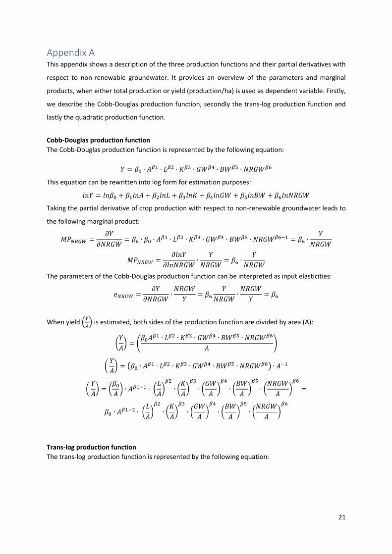
Appendix A This appendix shows a description of the three production functions and their partial derivatives with
respect to non-renewable groundwater. It provides an overview of the parameters and marginal
products, when either total production or yield (production/ha) is used as dependent variable. Firstly,
we describe the Cobb-Douglas production function, secondly the trans-log production function and
lastly the quadratic production function.
Cobb-Douglas production function
The Cobb-Douglas production function is represented by the following equation:
𝑌 = 𝛽0 ∙ 𝐴𝛽1 ∙ 𝐿𝛽2 ∙ 𝐾𝛽3 ∙ 𝐺𝑊𝛽4 ∙ 𝐵𝑊𝛽5 ∙ 𝑁𝑅𝐺𝑊𝛽6
This equation can be rewritten into log form for estimation purposes:
𝑙𝑛𝑌 = 𝑙𝑛𝛽0 + 𝛽1𝑙𝑛𝐴 + 𝛽2𝑙𝑛𝐿 + 𝛽3𝑙𝑛𝐾 + 𝛽4𝑙𝑛𝐺𝑊 + 𝛽5𝑙𝑛𝐵𝑊 + 𝛽6𝑙𝑛𝑁𝑅𝐺𝑊
Taking the partial derivative of crop production with respect to non-renewable groundwater leads to
the following marginal product:
𝑀𝑃𝑁𝑅𝐺𝑊 =𝜕𝑌
𝜕𝑁𝑅𝐺𝑊= 𝛽6 ∙ 𝛽0 ∙ 𝐴𝛽1 ∙ 𝐿𝛽2 ∙ 𝐾𝛽3 ∙ 𝐺𝑊𝛽4 ∙ 𝐵𝑊𝛽5 ∙ 𝑁𝑅𝐺𝑊𝛽6−1 = 𝛽6 ∙
𝑌
𝑁𝑅𝐺𝑊
𝑀𝑃𝑁𝑅𝐺𝑊 =𝜕𝑙𝑛𝑌
𝜕𝑙𝑛𝑁𝑅𝐺𝑊∙
𝑌
𝑁𝑅𝐺𝑊= 𝛽6 ∙
𝑌
𝑁𝑅𝐺𝑊
The parameters of the Cobb-Douglas production function can be interpreted as input elasticities:
𝑒𝑁𝑅𝐺𝑊 =𝜕𝑌
𝜕𝑁𝑅𝐺𝑊∙
𝑁𝑅𝐺𝑊
𝑌= 𝛽6
𝑌
𝑁𝑅𝐺𝑊∙
𝑁𝑅𝐺𝑊
𝑌= 𝛽6
When yield (𝑌
𝐴) is estimated, both sides of the production function are divided by area (A):
(𝑌
𝐴) = (
𝛽0𝐴𝛽1 ∙ 𝐿𝛽2 ∙ 𝐾𝛽3 ∙ 𝐺𝑊𝛽4 ∙ 𝐵𝑊𝛽5 ∙ 𝑁𝑅𝐺𝑊𝛽6
𝐴)
( 𝑌
𝐴) = (𝛽0 ∙ 𝐴𝛽1 ∙ 𝐿𝛽2 ∙ 𝐾𝛽3 ∙ 𝐺𝑊𝛽4 ∙ 𝐵𝑊𝛽5 ∙ 𝑁𝑅𝐺𝑊𝛽6) ∙ 𝐴−1
( 𝑌
𝐴) = (
𝛽0
𝐴) ∙ 𝐴𝛽1−1 ∙ (
𝐿
𝐴)
𝛽2
∙ (𝐾
𝐴)
𝛽3
∙ (𝐺𝑊
𝐴)
𝛽4
∙ (𝐵𝑊
𝐴)
𝛽5
∙ (𝑁𝑅𝐺𝑊
𝐴)
𝛽6
=
𝛽0 ∙ 𝐴𝛽1−2 ∙ (𝐿
𝐴)
𝛽2
∙ (𝐾
𝐴)
𝛽3
∙ (𝐺𝑊
𝐴)
𝛽4
∙ (𝐵𝑊
𝐴)
𝛽5
∙ (𝑁𝑅𝐺𝑊
𝐴)
𝛽6
Trans-log production function
The trans-log production function is represented by the following equation:
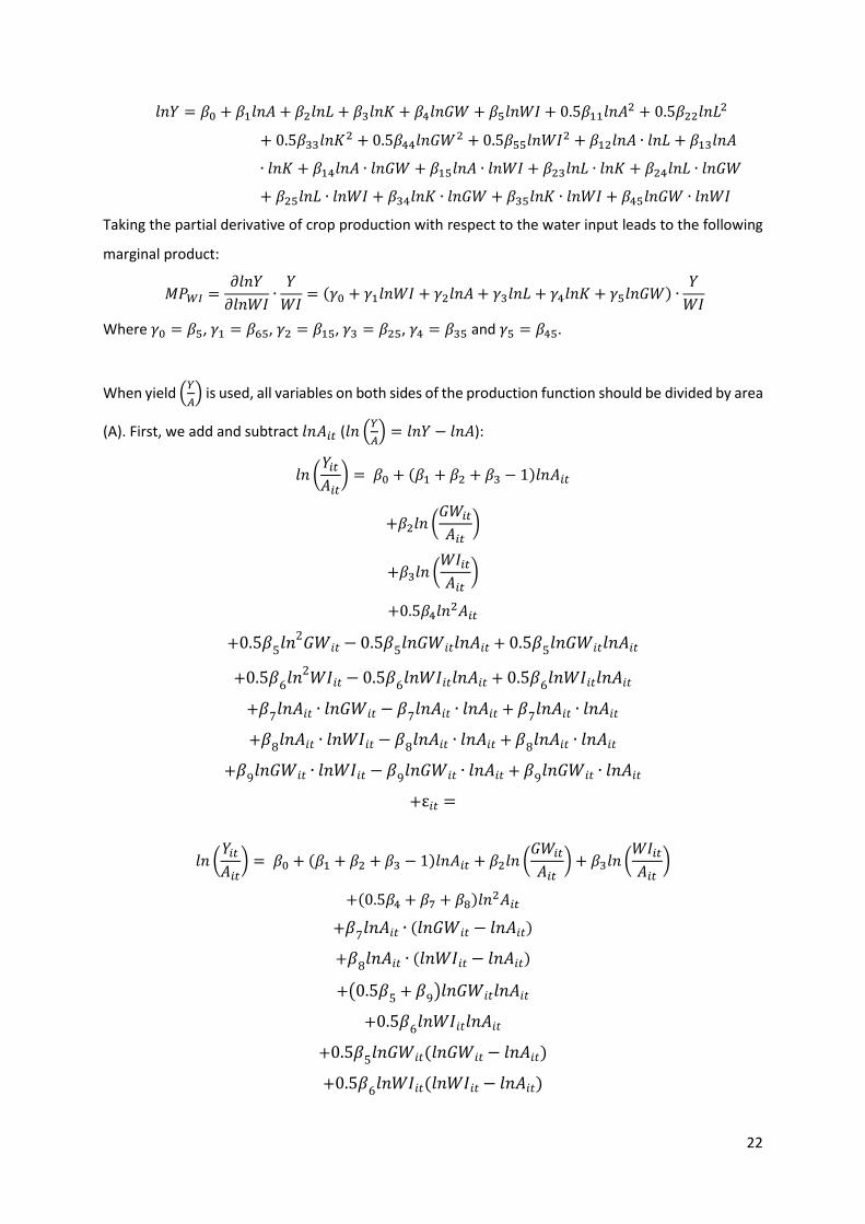
22
𝑙𝑛𝑌 = 𝛽0 + 𝛽1𝑙𝑛𝐴 + 𝛽2𝑙𝑛𝐿 + 𝛽3𝑙𝑛𝐾 + 𝛽4𝑙𝑛𝐺𝑊 + 𝛽5𝑙𝑛𝑊𝐼 + 0.5𝛽11𝑙𝑛𝐴2 + 0.5𝛽22𝑙𝑛𝐿2
+ 0.5𝛽33𝑙𝑛𝐾2 + 0.5𝛽44𝑙𝑛𝐺𝑊2 + 0.5𝛽55𝑙𝑛𝑊𝐼2 + 𝛽12𝑙𝑛𝐴 ∙ 𝑙𝑛𝐿 + 𝛽13𝑙𝑛𝐴
∙ 𝑙𝑛𝐾 + 𝛽14𝑙𝑛𝐴 ∙ 𝑙𝑛𝐺𝑊 + 𝛽15𝑙𝑛𝐴 ∙ 𝑙𝑛𝑊𝐼 + 𝛽23𝑙𝑛𝐿 ∙ 𝑙𝑛𝐾 + 𝛽24𝑙𝑛𝐿 ∙ 𝑙𝑛𝐺𝑊
+ 𝛽25𝑙𝑛𝐿 ∙ 𝑙𝑛𝑊𝐼 + 𝛽34𝑙𝑛𝐾 ∙ 𝑙𝑛𝐺𝑊 + 𝛽35𝑙𝑛𝐾 ∙ 𝑙𝑛𝑊𝐼 + 𝛽45𝑙𝑛𝐺𝑊 ∙ 𝑙𝑛𝑊𝐼
Taking the partial derivative of crop production with respect to the water input leads to the following
marginal product:
𝑀𝑃𝑊𝐼 =𝜕𝑙𝑛𝑌
𝜕𝑙𝑛𝑊𝐼∙
𝑌
𝑊𝐼= (𝛾0 + 𝛾1𝑙𝑛𝑊𝐼 + 𝛾2𝑙𝑛𝐴 + 𝛾3𝑙𝑛𝐿 + 𝛾4𝑙𝑛𝐾 + 𝛾5𝑙𝑛𝐺𝑊) ∙
𝑌
𝑊𝐼
Where 𝛾0 = 𝛽5, 𝛾1 = 𝛽65, 𝛾2 = 𝛽15, 𝛾3 = 𝛽25, 𝛾4 = 𝛽35 and 𝛾5 = 𝛽45.
When yield (𝑌
𝐴) is used, all variables on both sides of the production function should be divided by area
(A). First, we add and subtract 𝑙𝑛𝐴𝑖𝑡 (𝑙𝑛 (𝑌
𝐴) = 𝑙𝑛𝑌 − 𝑙𝑛𝐴):
𝑙𝑛 (𝑌𝑖𝑡
𝐴𝑖𝑡) = 𝛽0 + (𝛽1 + 𝛽2 + 𝛽3 − 1)𝑙𝑛𝐴𝑖𝑡
+𝛽2𝑙𝑛 (𝐺𝑊𝑖𝑡
𝐴𝑖𝑡)
+𝛽3𝑙𝑛 (𝑊𝐼𝑖𝑡
𝐴𝑖𝑡)
+0.5𝛽4𝑙𝑛2𝐴𝑖𝑡
+0.5𝛽5𝑙𝑛2𝐺𝑊𝑖𝑡 − 0.5𝛽5𝑙𝑛𝐺𝑊𝑖𝑡𝑙𝑛𝐴𝑖𝑡 + 0.5𝛽5𝑙𝑛𝐺𝑊𝑖𝑡𝑙𝑛𝐴𝑖𝑡
+0.5𝛽6𝑙𝑛2𝑊𝐼𝑖𝑡 − 0.5𝛽6𝑙𝑛𝑊𝐼𝑖𝑡𝑙𝑛𝐴𝑖𝑡 + 0.5𝛽6𝑙𝑛𝑊𝐼𝑖𝑡𝑙𝑛𝐴𝑖𝑡
+𝛽7𝑙𝑛𝐴𝑖𝑡 ∙ 𝑙𝑛𝐺𝑊𝑖𝑡 − 𝛽7𝑙𝑛𝐴𝑖𝑡 ∙ 𝑙𝑛𝐴𝑖𝑡 + 𝛽7𝑙𝑛𝐴𝑖𝑡 ∙ 𝑙𝑛𝐴𝑖𝑡
+𝛽8𝑙𝑛𝐴𝑖𝑡 ∙ 𝑙𝑛𝑊𝐼𝑖𝑡 − 𝛽8𝑙𝑛𝐴𝑖𝑡 ∙ 𝑙𝑛𝐴𝑖𝑡 + 𝛽8𝑙𝑛𝐴𝑖𝑡 ∙ 𝑙𝑛𝐴𝑖𝑡
+𝛽9𝑙𝑛𝐺𝑊𝑖𝑡 ∙ 𝑙𝑛𝑊𝐼𝑖𝑡 − 𝛽9𝑙𝑛𝐺𝑊𝑖𝑡 ∙ 𝑙𝑛𝐴𝑖𝑡 + 𝛽9𝑙𝑛𝐺𝑊𝑖𝑡 ∙ 𝑙𝑛𝐴𝑖𝑡
+ε𝑖𝑡 =
𝑙𝑛 (𝑌𝑖𝑡
𝐴𝑖𝑡) = 𝛽0 + (𝛽1 + 𝛽2 + 𝛽3 − 1)𝑙𝑛𝐴𝑖𝑡 + 𝛽2𝑙𝑛 (
𝐺𝑊𝑖𝑡
𝐴𝑖𝑡) + 𝛽3𝑙𝑛 (
𝑊𝐼𝑖𝑡
𝐴𝑖𝑡)
+(0.5𝛽4 + 𝛽7 + 𝛽8)𝑙𝑛2𝐴𝑖𝑡
+𝛽7𝑙𝑛𝐴𝑖𝑡 ∙ (𝑙𝑛𝐺𝑊𝑖𝑡 − 𝑙𝑛𝐴𝑖𝑡)
+𝛽8𝑙𝑛𝐴𝑖𝑡 ∙ (𝑙𝑛𝑊𝐼𝑖𝑡 − 𝑙𝑛𝐴𝑖𝑡)
+(0.5𝛽5 + 𝛽9)𝑙𝑛𝐺𝑊𝑖𝑡𝑙𝑛𝐴𝑖𝑡
+0.5𝛽6𝑙𝑛𝑊𝐼𝑖𝑡𝑙𝑛𝐴𝑖𝑡
+0.5𝛽5𝑙𝑛𝐺𝑊𝑖𝑡(𝑙𝑛𝐺𝑊𝑖𝑡 − 𝑙𝑛𝐴𝑖𝑡)
+0.5𝛽6𝑙𝑛𝑊𝐼𝑖𝑡(𝑙𝑛𝑊𝐼𝑖𝑡 − 𝑙𝑛𝐴𝑖𝑡)

23
+𝛽9𝑙𝑛𝐺𝑊𝑖𝑡 ∙ (𝑙𝑛𝑊𝐼𝑖𝑡 − 𝑙𝑛𝐴𝑖𝑡)
+ε𝑖𝑡
Next, we divide the remaining terms by area:
𝑙𝑛 (𝑌𝑖𝑡
𝐴𝑖𝑡) = 𝛽0 + (𝛽1 + 𝛽2 + 𝛽3 − 1)𝑙𝑛𝐴𝑖𝑡 + 𝛽2𝑙𝑛 (
𝐺𝑊𝑖𝑡
𝐴𝑖𝑡) + 𝛽3𝑙𝑛 (
𝑊𝐼𝑖𝑡
𝐴𝑖𝑡)
+(0.5𝛽4 + 𝛽7 + 𝛽8)𝑙𝑛2𝐴𝑖𝑡
+𝛽7𝑙𝑛𝐴𝑖𝑡 ∙ (𝑙𝑛𝐺𝑊𝑖𝑡 − 𝑙𝑛𝐴𝑖𝑡)
+𝛽8𝑙𝑛𝐴𝑖𝑡 ∙ (𝑙𝑛𝑊𝐼𝑖𝑡 − 𝑙𝑛𝐴𝑖𝑡)
+(0.5𝛽5 + 𝛽9)𝑙𝑛𝐺𝑊𝑖𝑡𝑙𝑛𝐴𝑖𝑡 − (0.5𝛽5 + 𝛽9)𝑙𝑛𝐴𝑖𝑡𝑙𝑛𝐴𝑖𝑡 + (0.5𝛽5 + 𝛽9)𝑙𝑛𝐴𝑖𝑡𝑙𝑛𝐴𝑖𝑡
+0.5𝛽6𝑙𝑛𝑊𝐼𝑖𝑡𝑙𝑛𝐴𝑖𝑡 − (0.5𝛽6)𝑙𝑛𝐴𝑖𝑡𝑙𝑛𝐴𝑖𝑡 + (0.5𝛽6)𝑙𝑛𝐴𝑖𝑡𝑙𝑛𝐴𝑖𝑡
+0.5𝛽5𝑙𝑛𝐺𝑊𝑖𝑡(𝑙𝑛𝐺𝑊𝑖𝑡 − 𝑙𝑛𝐴𝑖𝑡) − 0.5𝛽5𝑙𝑛𝐴𝑖𝑡(𝑙𝑛𝐺𝑊𝑖𝑡 − 𝑙𝑛𝐴𝑖𝑡)
+ 0.5𝛽5𝑙𝑛𝐴𝑖𝑡(𝑙𝑛𝐺𝑊𝑖𝑡 − 𝑙𝑛𝐴𝑖𝑡)
+0.5𝛽6𝑙𝑛𝑊𝐼𝑖𝑡(𝑙𝑛𝑊𝐼𝑖𝑡 − 𝑙𝑛𝐴𝑖𝑡) − 0.5𝛽6𝑙𝑛𝐴𝑖𝑡(𝑙𝑛𝑊𝐼𝑖𝑡 − 𝑙𝑛𝐴𝑖𝑡) + 0.5𝛽6𝑙𝑛𝐴𝑖𝑡(𝑙𝑛𝑊𝐼𝑖𝑡 − 𝑙𝑛𝐴𝑖𝑡)
+𝛽9𝑙𝑛𝐺𝑊𝑖𝑡 ∙ (𝑙𝑛𝑊𝐼𝑖𝑡 − 𝑙𝑛𝐴𝑖𝑡) − 𝛽9𝑙𝑛𝐴𝑖𝑡 ∙ (𝑙𝑛𝑊𝐼𝑖𝑡 − 𝑙𝑛𝐴𝑖𝑡) + 𝛽9𝑙𝑛𝐴𝑖𝑡 ∙ (𝑙𝑛𝑊𝐼𝑖𝑡 − 𝑙𝑛𝐴𝑖𝑡)
+ε𝑖𝑡 =
𝑙𝑛 (𝑌𝑖𝑡
𝐴𝑖𝑡) = 𝛽0 + (𝛽1 + 𝛽2 + 𝛽3 − 1)𝑙𝑛𝐴𝑖𝑡 + 𝛽2𝑙𝑛 (
𝐺𝑊𝑖𝑡
𝐴𝑖𝑡) + 𝛽3𝑙𝑛 (
𝑊𝐼𝑖𝑡
𝐴𝑖𝑡)
+(0.5𝛽4 + 𝛽7 + 𝛽8)𝑙𝑛2𝐴𝑖𝑡
+𝛽7𝑙𝑛𝐴𝑖𝑡 ∙ (𝑙𝑛𝐺𝑊𝑖𝑡 − 𝑙𝑛𝐴𝑖𝑡)
+𝛽8𝑙𝑛𝐴𝑖𝑡 ∙ (𝑙𝑛𝑊𝐼𝑖𝑡 − 𝑙𝑛𝐴𝑖𝑡)
+(0.5𝛽5 + 𝛽9)(𝑙𝑛𝐺𝑊𝑖𝑡 − 𝑙𝑛𝐴𝑖𝑡)𝑙𝑛𝐴𝑖𝑡 + (0.5𝛽5 + 𝛽9)𝑙𝑛𝐴𝑖𝑡𝑙𝑛𝐴𝑖𝑡
+(0.5𝛽6)(𝑙𝑛𝑊𝐼𝑖𝑡 − 𝑙𝑛𝐴𝑖𝑡)𝑙𝑛𝐴𝑖𝑡 + (0.5𝛽6)𝑙𝑛𝐴𝑖𝑡𝑙𝑛𝐴𝑖𝑡
+0.5𝛽5(𝑙𝑛𝐺𝑊𝑖𝑡 − 𝑙𝑛𝐴𝑖𝑡)(𝑙𝑛𝐺𝑊𝑖𝑡 − 𝑙𝑛𝐴𝑖𝑡) + 0.5𝛽5𝑙𝑛𝐴𝑖𝑡(𝑙𝑛𝐺𝑊𝑖𝑡 − 𝑙𝑛𝐴𝑖𝑡)
+0.5𝛽6(𝑙𝑛𝑊𝐼𝑖𝑡 − 𝑙𝑛𝐴𝑖𝑡)(𝑙𝑛𝑊𝐼𝑖𝑡 − 𝑙𝑛𝐴𝑖𝑡) + 0.5𝛽6𝑙𝑛𝐴𝑖𝑡(𝑙𝑛𝑊𝐼𝑖𝑡 − 𝑙𝑛𝐴𝑖𝑡)
+𝛽9(𝑙𝑛𝐺𝑊𝑖𝑡 − 𝑙𝑛𝐴𝑖𝑡) (𝑙𝑛𝑊𝐼𝑖𝑡 − 𝑙𝑛𝐴𝑖𝑡) + 𝛽9𝑙𝑛𝐴𝑖𝑡 ∙ (𝑙𝑛𝑊𝐼𝑖𝑡 − 𝑙𝑛𝐴𝑖𝑡)
+ε𝑖𝑡 =
𝑙𝑛 (𝑌𝑖𝑡
𝐴𝑖𝑡) = 𝛽0 + (𝛽1 + 𝛽2 + 𝛽3 − 1)𝑙𝑛𝐴𝑖𝑡 + 𝛽2𝑙𝑛 (
𝐺𝑊𝑖𝑡
𝐴𝑖𝑡) + 𝛽3𝑙𝑛 (
𝑊𝐼𝑖𝑡
𝐴𝑖𝑡)
+(0.5𝛽4 + 𝛽7 + 𝛽8 + 0.5𝛽5 + 𝛽9 + 0.5𝛽6)𝑙𝑛2𝐴𝑖𝑡
+(𝛽7 + 𝛽5 + 𝛽9)(𝑙𝑛𝐺𝑊𝑖𝑡 − 𝑙𝑛𝐴𝑖𝑡)𝑙𝑛𝐴𝑖𝑡

24
+(𝛽8 + 𝛽6 + 𝛽9)(𝑙𝑛𝑊𝐼𝑖𝑡 − 𝑙𝑛𝐴𝑖𝑡)𝑙𝑛𝐴𝑖𝑡
+0.5𝛽5(𝑙𝑛𝐺𝑊𝑖𝑡 − 𝑙𝑛𝐴𝑖𝑡)(𝑙𝑛𝐺𝑊𝑖𝑡 − 𝑙𝑛𝐴𝑖𝑡)
+0.5𝛽6(𝑙𝑛𝑊𝐼𝑖𝑡 − 𝑙𝑛𝐴𝑖𝑡)(𝑙𝑛𝑊𝐼𝑖𝑡 − 𝑙𝑛𝐴𝑖𝑡)
+𝛽9(𝑙𝑛𝐺𝑊𝑖𝑡 − 𝑙𝑛𝐴𝑖𝑡) (𝑙𝑛𝑊𝐼𝑖𝑡 − 𝑙𝑛𝐴𝑖𝑡)
+ε𝑖𝑡 =
𝑙𝑛 (𝑌𝑖𝑡
𝐴𝑖𝑡) = 𝛽0 + (𝛽1 + 𝛽2 + 𝛽3 − 1)𝑙𝑛𝐴𝑖𝑡 + 𝛽2𝑙𝑛 (
𝐺𝑊𝑖𝑡
𝐴𝑖𝑡) + 𝛽3𝑙𝑛 (
𝑊𝐼𝑖𝑡
𝐴𝑖𝑡)
+(0.5𝛽4 + 𝛽7 + 𝛽8 + 0.5𝛽5 + 𝛽9 + 0.5𝛽6)𝑙𝑛2𝐴𝑖𝑡
+(𝛽7 + 𝛽5 + 𝛽9) (𝑙𝑛𝐺𝑊𝑖𝑡
𝑙𝑛𝐴𝑖𝑡) 𝑙𝑛𝐴𝑖𝑡
+(𝛽8 + 𝛽6 + 𝛽9) (𝑙𝑛𝑊𝐼𝑖𝑡
𝑙𝑛𝐴𝑖𝑡) 𝑙𝑛𝐴𝑖𝑡
+0.5𝛽5 (𝑙𝑛𝐺𝑊𝑖𝑡
𝑙𝑛𝐴𝑖𝑡)
2
+0.5𝛽6 (𝑙𝑛𝑊𝐼𝑖𝑡
𝑙𝑛𝐴𝑖𝑡)
2
+𝛽9 (𝑙𝑛𝐺𝑊𝑖𝑡
𝑙𝑛𝐴𝑖𝑡) (
𝑙𝑛𝑊𝐼𝑖𝑡
𝑙𝑛𝐴𝑖𝑡)
+ε𝑖𝑡 =
𝑙𝑛 (𝑌𝑖𝑡
𝐴𝑖𝑡) = 𝛾0 + 𝛾1𝑙𝑛𝐴𝑖𝑡 + 𝛾2 (
𝑙𝑛𝐺𝑊𝑖𝑡
𝑙𝑛𝐴𝑖𝑡) + 𝛾3 (
𝑙𝑛𝑊𝐼𝑖𝑡
𝑙𝑛𝐴𝑖𝑡) + 𝛾4𝑙𝑛2𝐴𝑖𝑡 + 𝛾5 (
𝑙𝑛𝐺𝑊𝑖𝑡
𝑙𝑛𝐴𝑖𝑡) 𝑙𝑛𝐴𝑖𝑡
+ 𝛾6 (𝑙𝑛𝑊𝐼𝑖𝑡
𝑙𝑛𝐴𝑖𝑡) 𝑙𝑛𝐴𝑖𝑡 + 𝛾7 (
𝑙𝑛𝐺𝑊𝑖𝑡
𝑙𝑛𝐴𝑖𝑡)
2
+ 𝛾8 (𝑙𝑛𝑊𝐼𝑖𝑡
𝑙𝑛𝐴𝑖𝑡)
2
+ 𝛾9 (𝑙𝑛𝐺𝑊𝑖𝑡
𝑙𝑛𝐴𝑖𝑡) (
𝑙𝑛𝑊𝐼𝑖𝑡
𝑙𝑛𝐴𝑖𝑡)
+ ε𝑖𝑡
Where 𝛾0 = 𝛽0, 𝛾1 = (𝛽1 + 𝛽2 + 𝛽3 − 1), 𝛾2 = 𝛽2, 𝛾3 = 𝛽3, 𝛾4 = (0.5𝛽4 + 𝛽7 + 𝛽8 + 0.5𝛽5 + 𝛽9 +
0.5𝛽6), 𝛾5 = (𝛽7 + 𝛽5 + 𝛽9), 𝛾6 = (𝛽8 + 𝛽6 + 𝛽9), 𝛾7 = 0.5𝛽5, 𝛾8 = 0.5𝛽6 and 𝛾9 = 𝛽9.
Taking the partial derivative of yield with respect to the water input per hectare gives the following
marginal product:
𝑀𝑃𝑊𝐼 =𝜕𝑙𝑛 (
𝑌𝐴)
𝜕𝑙𝑛 (𝑊𝐼𝐴 )
∙(
𝑌𝐴)
(𝑊𝐼𝐴 )
= 𝛾3 + 𝛾6𝑙𝑛𝐴 + 2𝛾8𝑙𝑛 (𝑊𝐼
𝐴) + 𝛾9𝑙𝑛 (
𝐺𝑊
𝐴) ∙
(𝑌𝐴)
(𝑊𝐼𝐴 )

25
Quadratic production function
The quadratic production function is represented by the following equation:
𝑌 = 𝛽0 + 𝛽1𝐴 + 𝛽2𝐴2 + 𝛽3𝐿 + 𝛽4𝐿2 + 𝛽5𝐾 + 𝛽6𝐾2 + 𝛽7𝐺𝑊 + 𝛽8𝐺𝑊2 + 𝛽9𝑊𝐼 + 𝛽10𝑊𝐼2 + 𝛽11𝐴
∙ 𝐿 + 𝛽12𝐴 ∙ 𝐾 + 𝛽13𝐴 ∙ 𝐺𝑊 + 𝛽14𝐴 ∙ 𝑊𝐼 + 𝛽15𝐿 ∙ 𝐾 + 𝛽16𝐿 ∙ 𝐺𝑊 + 𝛽17𝐿 ∙ 𝑊𝐼
+ 𝛽18𝐾 ∙ 𝐺𝑊 + 𝛽19𝐾 ∙ 𝑊𝐼 + 𝛽20𝐺𝑊 ∙ 𝑊𝐼
Taking the partial derivative of crop production with respect to the water input leads to the following
marginal product:
𝑀𝑃𝑁𝑅𝑊𝐼 =𝜕𝑌
𝜕𝑊𝐼= 𝛾0 + 𝛾1𝑊𝐼 + 𝛾2𝐴 + 𝛾3𝐿 + 𝛾4𝐾 + 𝛾5𝐺𝑊
Where 𝛾0 = 𝛽9, 𝛾1 = 2𝛽10, 𝛾2 = 𝛽14, 𝛾3 = 𝛽17, 𝛾4 = 𝛽19 and 𝛾5 = 𝛽20.
When yield (𝑌
𝐴) is used, both sides of the production function are divided by area (A):
(𝑌
𝐴) = (
𝛽0
𝐴) + 𝛽1 (
𝐴
𝐴) + 𝛽2 (
𝐴
𝐴)
2
+ 𝛽3 (𝐿
𝐴) + 𝛽4 (
𝐿
𝐴)
2
+ 𝛽5 (𝐾
𝐴) + 𝛽6 (
𝐾
𝐴)
2
+ 𝛽7 (𝐺𝑊
𝐴) + 𝛽8 (
𝐺𝑊
𝐴)
2
+ 𝛽9 (𝑊𝐼
𝐴) + 𝛽10 (
𝑊𝐼
𝐴)
2
+ 𝛽11 (𝐴
𝐴) ∙ (
𝐿
𝐴) + 𝛽12 (
𝐴
𝐴) ∙ (
𝐾
𝐴) + 𝛽13 (
𝐴
𝐴) ∙ (
𝐺𝑊
𝐴)
+ 𝛽14 (𝐴
𝐴) ∙ (
𝑊𝐼
𝐴) + 𝛽15 (
𝐿
𝐴) ∙ (
𝐾
𝐴) + 𝛽16 (
𝐿
𝐴) ∙ (
𝐺𝑊
𝐴) + 𝛽17 (
𝐿
𝐴) ∙ (
𝑊𝐼
𝐴) + 𝛽18 (
𝐾
𝐴)
∙ (𝐺𝑊
𝐴) + 𝛽19 (
𝐾
𝐴) ∙ (
𝑊𝐼
𝐴) + 𝛽20 (
𝐺𝑊
𝐴) ∙ (
𝑊𝐼
𝐴) =
(𝑌
𝐴) = (
𝛽0
𝐴) + (𝛽1 + 𝛽2) + 𝛽3 (
𝐿
𝐴) + 𝛽4 (
𝐿
𝐴)
2
+ 𝛽5 (𝐾
𝐴) + 𝛽6 (
𝐾
𝐴)
2
+ 𝛽7 (𝐺𝑊
𝐴) + 𝛽8 (
𝐺𝑊
𝐴)
2
+ 𝛽9 (𝑊𝐼
𝐴) + 𝛽10 (
𝑊𝐼
𝐴)
2
+ 𝛽11 (𝐴
𝐴) ∙ (
𝐿
𝐴) + 𝛽12 (
𝐴
𝐴) ∙ (
𝐾
𝐴) + 𝛽13 (
𝐴
𝐴) ∙ (
𝐺𝑊
𝐴)
+ 𝛽14 (𝐴
𝐴) ∙ (
𝑊𝐼
𝐴) + 𝛽15 (
𝐿
𝐴) ∙ (
𝐾
𝐴) + 𝛽16 (
𝐿
𝐴) ∙ (
𝐺𝑊
𝐴) + 𝛽17 (
𝐿
𝐴) ∙ (
𝑊𝐼
𝐴) + 𝛽18 (
𝐾
𝐴)
∙ (𝐺𝑊
𝐴) + 𝛽19 (
𝐾
𝐴) ∙ (
𝑊𝐼
𝐴) + 𝛽20 (
𝐺𝑊
𝐴) ∙ (
𝑊𝐼
𝐴)
Taking the partial derivative of yield with respect to the water input per hectare leads to the following
marginal product:
𝑀𝑃𝑁𝑅𝐺𝑊 =𝜕 (
𝑌𝐴
)
𝜕 (𝑁𝑅𝐺𝑊
𝐴 )= 𝛾0 + 𝛾1 (
𝑊𝐼
𝐴) + 𝛾2 (
𝐴
𝐴) + 𝛾3 (
𝐿
𝐴) + 𝛾4 (
𝐾
𝐴) + 𝛾5 (
𝐺𝑊
𝐴)
Where 𝛾0 = 𝛽9, 𝛾1 = 2𝛽10, 𝛾2 = 𝛽14, 𝛾3 = 𝛽17, 𝛾4 = 𝛽19 and 𝛾5 = 𝛽20.

26
Appendix B Overview of the ten most important crops produced per country (1000 tonnes), based on FAO
(2016a):
Overview of crop production of India, Italy, Saudi Arabia, Spain and Turkey, based on FAO (2016a):
China Egypt India Iran Italy Mexico
rice 7618477 sugarcane 545520 sugarcane 10380218 wheat 389700 sugarbeet 469532 sugarcane 1908256
maize 4605872 maize 218993 rice 4883753 sugarbeet 195320 grapes 423516 maize 701844
wheat 3885583 wheat 209482 wheat 2488556 potatoes 119337 wheat 369367 sorghum 235927
sugarcane 2816625 rice 182485 potatoes 851666 sugarcane 118492 maize 342143 citrus 193877
potatoes 2117499 sugarbeet 99347 pulses 549034 barley 105994 citrus 132437 wheat 152455
soybeans 532829 citrus 91411 maize 499044 citrus 95793 potatoes 102576 oranges 124752
groundnuts 385108 potatoes 87927 millet 455181 rice 89777 oranges 81200 pulses 61312
sugarbeet 383230 oranges 65160 sorghum 409950 grapes 75516 rice 54770 potatoes 53152
citrus 383085 sorghum 33757 groundnuts 303164 oranges 52789 barley 50979 lemons 48573
pulses 234736 dates 33282 chick_peas 246636 maize 33766 lemons 28103 beans_dry 47558
Pakistan Saudi Arabia South Africa Spain Turkey USA
sugarcane 1818223 wheat 71039 sugarcane 830753 barley 353128 wheat 807912 maize 9939061
wheat 694647 dates 26722 maize 420585 sugarbeet 305093 sugarbeet 567777 soybeans 2807977
rice 260722 potatoes 8827 wheat 90526 grapes 242389 barley 296971 wheat 2638283
maize 80514 barley 8657 potatoes 59500 wheat 235746 potatoes 178128 sugarcane 1224835
citrus 66531 sorghum 7282 grapes 57379 citrus 196454 grapes 157945 sugarbeet 1156796
cotton 61513 grapes 4158 citrus 55294 potatoes 188185 maize 108172 potatoes 819369
potatoes 56996 citrus 2979 oranges 39360 maize 141687 citrus 81887 sorghum 695640
oranges 46634 citrus_fruit_nes2979 sunflower 21763 oranges 105938 pulses 60013 citrus 537170
pulses 33327 maize 1375 sorghum 16776 tangerines 63106 oranges 41563 oranges 386555
chick_peas 24529 groundnuts 99 grapefruit 8131 sunflower 34926 sunflower 38275 barley 351470
0100000000200000000300000000400000000500000000600000000700000000800000000900000000
1E+09
19
70
19
72
19
74
19
76
19
78
19
80
19
82
19
84
19
86
19
88
19
90
19
92
19
94
19
96
19
98
20
00
20
02
20
04
20
06
20
08
20
10
20
12
Pro
du
ctio
n (
ton
s)
Year
Crop production India (1970-2012)
sugarcane rice wheat other_crops perennial_other
potatoes pulses maize millet sorghum
groundnuts chick_peas soybeans citrus beans_dry
pigeon_peas oranges cotton barley lemons
grapes lentils sunflower peas coffee
citrus_fruit_nes grapefruit cocoa

27
0
10000000
20000000
30000000
40000000
50000000
60000000
70000000
80000000
90000000
19
70
19
72
19
74
19
76
19
78
19
80
19
82
19
84
19
86
19
88
19
90
19
92
19
94
19
96
19
98
20
00
20
02
20
04
20
06
20
08
20
10
20
12
Pro
du
ctio
n (
ton
s)
Year
Crop production Italy (1970-2013)
other_crops sugarbeet grapes perennial_other wheat
maize citrus potatoes oranges rice
barley lemons soybeans tangerines sunflower
pulses broad_beans sorghum beans_dry citrus_fruit_nes
rye peas chick_peas vetches lupins
grapefruit lentils groundnuts
0
1000000
2000000
3000000
4000000
5000000
6000000
7000000
8000000
9000000
19
70
19
72
19
74
19
76
19
78
19
80
19
82
19
84
19
86
19
88
19
90
19
92
19
94
19
96
19
98
20
00
20
02
20
04
20
06
20
08
20
10
20
12
Pro
du
ctio
n (
ton
s)
Year
Crop production Saudi Arabia (1970-2012)
wheat other_crops dates potatoes
barley perennial_other sorghum grapes
citrus citrus_fruit_nes maize groundnuts

28
0
10000000
20000000
30000000
40000000
50000000
60000000
70000000
80000000
19
70
19
72
19
74
19
76
19
78
19
80
19
82
19
84
19
86
19
88
19
90
19
92
19
94
19
96
19
98
20
00
20
02
20
04
20
06
20
08
20
10
20
12
Pro
du
ctio
n (
ton
s)
Year
Crop production Spain (1970-2012)
barley perennial_other other_crops sugarbeet grapes
wheat citrus potatoes maize oranges
tangerines sunflower rice lemons pulses
rye sugarcane sorghum cotton peas
vetches broad_beans beans_dry chick_peas lentils
grapefruit dates soybeans citrus_fruit_nes lupins
groundnuts
0
20000000
40000000
60000000
80000000
100000000
120000000
19
70
19
72
19
74
19
76
19
78
19
80
19
82
19
84
19
86
19
88
19
90
19
92
19
94
19
96
19
98
20
00
20
02
20
04
20
06
20
08
20
10
20
12
Pro
du
ctio
n (
ton
s)
Year
Crop production Turkey (1970-2012)
wheat other_crops sugarbeet barley perennial_other
potatoes grapes maize citrus pulses
oranges sunflower cotton chick_peas lentils
lemons tangerines rice rye beans_dry
vetches grapefruit groundnuts soybeans broad_beans
dates citrus_fruit_nes peas sorghum

29
Appendix C This appendix contains panel graphs and panel unit root tests for the variables of citrus, maize and
sugarcane. The panel unit root test is shown for citrus production and performed in the same way for
the other variables. The table below gives a summary of the outcomes: yes means that the data are
stationary and no means that the data are nonstationary.
*Yes/No: Dependent on including a trend in the test or not. May be caused by country 100 (India)
which deviates from rest of the countries in case of sugarcane.
In the graphs, the countries are represented by numbers:
41 China 165 Pakistan
59 Egypt 194 Saudi Arabia
100 India 202 South Africa
102 Iran 203 Spain
106 Italy 223 Turkey
138 Mexico 231 USA
Citrus
0
5000000
10000000
15000000
20000000
25000000
Pro
du
ction
0 10 20 30 40group(Year)
Country = 41 Country = 59
Country = 102 Country = 106
Country = 138 Country = 165
Country = 194 Country = 202
Country = 203 Country = 223
Country = 231
Citrus Maize Sugarcane
Variables Original Ln Original Ln Original Ln
Production No Yes No No Yes/No* Yes
Yield No Yes No Yes Yes Yes
Green water No Yes Yes Yes Yes/No* Yes
Blue water No Yes No Yes No No
Non-renewable groundwater
No Yes Yes/No* Yes Yes/No*
No

30

31

32
Maize
0
1.000e+08
2.000e+08
3.000e+08
4.000e+08
Pro
du
ction
0 10 20 30 40group(Year)
Country = 41 Country = 59
Country = 100 Country = 102
Country = 106 Country = 138
Country = 165 Country = 194
Country = 202 Country = 203
Country = 223 Country = 231

33

34
35
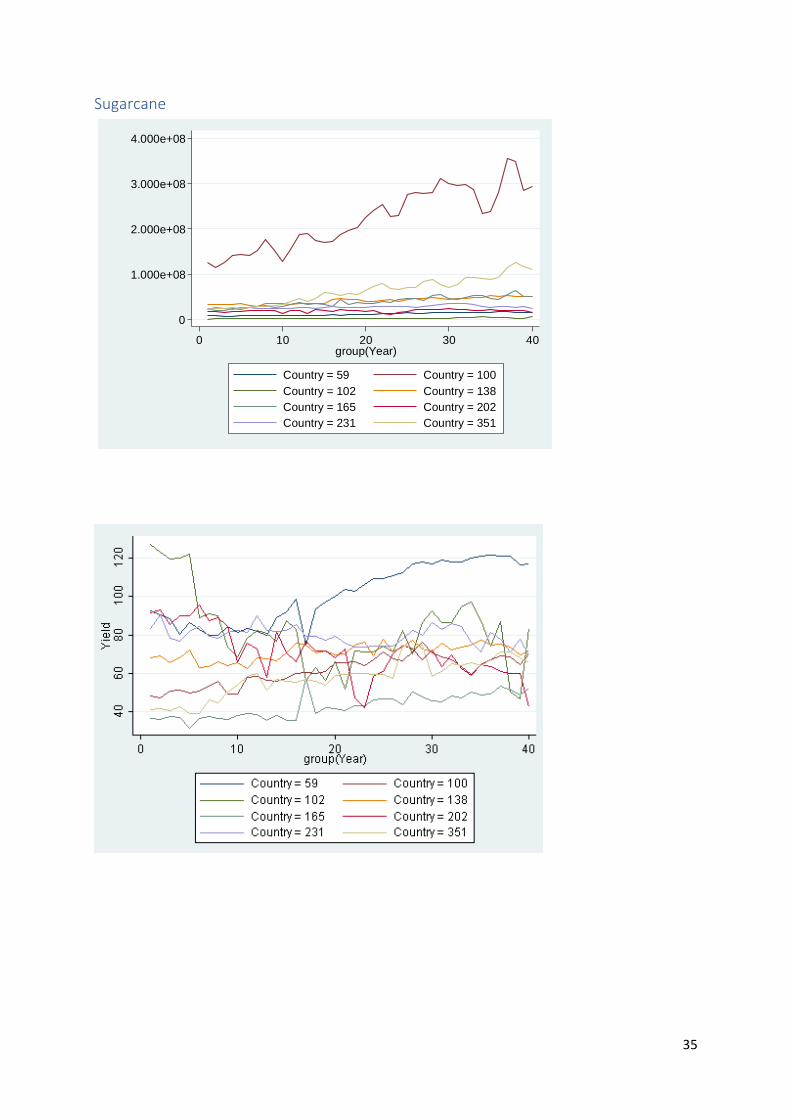
Sugarcane
0
1.000e+08
2.000e+08
3.000e+08
4.000e+08
Pro
du
ction
0 10 20 30 40group(Year)
Country = 59 Country = 100
Country = 102 Country = 138
Country = 165 Country = 202
Country = 231 Country = 351

36

37

38
Appendix D This appendix contains the correlation coefficient tables, including the quadratic terms and cross
terms, for the variables of citrus, maize and sugarcane.
Citrus
Maize
Sugarcane

39

40
Appendix E This appendix contains the OLS regression results for citrus and maize of the four countries together.
The estimations include the proxy variables for some inputs (mentioned in Chapter 4).
Citrus

41
Maize
Sugarcane
Italy and Spain do not produce sugarcane, so the estimation could include only South Africa and the
USA. Due to insufficient observations, no estimation for sugarcane can be performed.
42
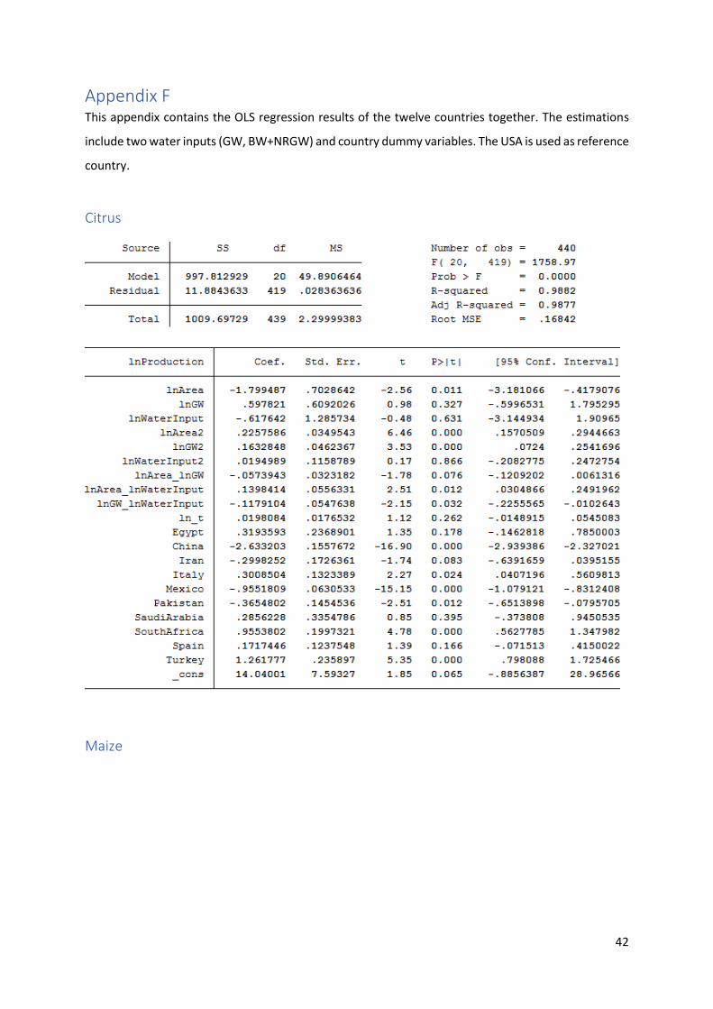
Appendix F This appendix contains the OLS regression results of the twelve countries together. The estimations
include two water inputs (GW, BW+NRGW) and country dummy variables. The USA is used as reference
country.
Citrus
Maize

43

44
Sugarcane

45
Appendix G This appendix contains the panel estimation results by including two water inputs (GW, BW+NRGW)
for production and yield estimation of citrus, maize and sugarcane.
Citrus
Production

46
Yield
Maize
Production

47
Yield
Sugarcane
Production
Yield

48
Cobb Douglas

49
Appendix H This appendix contains the calculated shadow prices per year for the countries included in the
estimation of citrus, maize and sugarcane yield.
Citrus
Maize
1991 1992 1993 1994 1995 1996 1997 1998 1999 2000 2001 2002 2003 2004 2005 2006 2007 2008 2009 2010 2011 2012 2013
Iran 0,678715 1,145815 0,128727 0,1418187 0,358392 0,469977 0,4538105 0,594121 0,887446 0,85213 0,840424 0,30308 0,276793 0,206956 0,25188 0,307191 0,37885 0,396143 0,488574 0,537966 0,600141 0,935176 0,811308
Italy 0,661861 0,567946 0,388126 0,3686698 0,402193 0,434209 0,3831434 0,362305 0,387411 0,307337 0,323632 0,367775 0,46751 0,488933 0,440581 0,44858 0,517156 0,442244 0,493536 0,464743 0,511121 0,458629 0,536529
Mexico 0,203355 0,191301 0,193511 0,1233311 0,089844 0,107091 0,1002737 0,125156 0,157455 0,132468 0,095894 0,105171 0,114225 0,101887 0,094922 0,117933 0,137641 0,12938 0,114848 0,142619 0,166623 0,152591 0,148573
Pakistan 0,104501 0,101088 0,129277 0,1451964 0,12747 0,11456 0,116057 0,114863 0,067366 0,099207 0,081982 0,159772 0,190191 0,191802 0,188917 0,211241 0,209273 0,191299 0,191962 0,201755
Saudi Arabia 0,768866 0,711913 0,797343 0,711913 0,711913
South Africa0,220348 0,242068 0,23792 0,2278053 0,325127 0,243541 0,196686 0,242287 0,225565 0,137097 0,164727 0,145005 0,235703 0,30939 0,204457 0,222464 0,317044 0,32657 0,270175 0,434495 0,487713 0,437525 0,297762
Spain 0,308215 0,262712 0,185368 0,261328 0,372941 0,42272 0,2910872 0,259563 0,272248 0,213062 0,22142 0,23183 0,275274 0,305148 0,316889 0,238851 0,296029 0,416176 0,335821 0,367958 0,309194 0,265858 0,316204
Turkey 0,329884 0,321137 0,339755 0,2776004 0,387099 0,401926 0,343936 0,336166 0,310479 0,305252 0,207955 0,244284 0,336092 0,400936 0,472564 0,428539 0,558318 0,621452 0,486354 0,520909 0,471448 0,424748 0,354756
USA 0,249595 0,22285 0,16287 0,1794977 0,170819 0,191379 0,1715958 0,118215 0,154873 0,114662 0,108144 0,128475 0,10817 0,113925 0,160291 0,194806 0,353178 0,220084 0,191151 0,233958 0,250868 0,381135 0,339301
China 0,068882 0,065811 0,05601 0,0475197 0,041523 0,0843 0,0218977 0,096728 0,134938 0,13472 0,122869 0,129982 0,108871 0,119356 0,122658 0,162936 0,476663 0,648864 0,632894 0,538113 0,652762 0,613001 0,755788
Egypt 0,11351 0,1155452 0,112645 0,127932 0,1344745 0,136487 0,136485 0,135539 0,116911 0,105348 0,081939 0,082285 0,09038 0,146855 0,197373 0,154367 0,286307 0,194937 0,192247 0,189297 0,167366
1991 1992 1993 1994 1995 1996 1997 1998 1999 2000 2001 2002 2003 2004 2005 2006 2007 2008 2009 2010 2011 2012 2013
India 0,150624 0,133127 0,116694 0,12977 0,129984 0,118651 0,12228868 0,121135 0,12782 0,119692 0,107842 0,113747 0,116694 0,142219 0,138084 0,182808 0,210199 0,208515
Iran 0,218946 0,191323 0,149014 0,184363 0,264377 0,26374327 0,337815 0,556439 0,540021 0,551066 0,165189 0,158421 0,159956 0,172845 0,193735 0,262596 0,269145 0,263248 0,299017 0,430771 0,52182 0,518286
Italy 0,327155 0,290649 0,232137 0,214883 0,254043 0,247059 0,18515155 0,174153 0,179486 0,141185 0,134456 0,130501 0,165153 0,193885 0,169109 0,186317 0,268953 0,295661 0,196939 0,238581 0,34153 0,311521 0,323584
Mexico 0,252951 0,265544 0,266205 0,209901 0,183707 0,203924 0,18466164 0,170926 0,164243 0,172232 0,16773 0,167874 0,161955 0,16071 0,156433 0,199296 0,241343 0,273339 0,224321 0,240827 0,355717 0,329036 0,284737
Pakistan 0,208222 0,196201 0,175282 0,200643 0,22614 0,21393 0,22480574 0,209051 0,177129 0,161362 0,14401 0,151891 0,165024 0,187187 0,183537 0,197122 0,204474 0,180992 0,235661 0,247249
South Africa0,139621 0,171153 0,13616 0,111011 0,171797 0,148702 0,13827443 0,11213 0,119139 0,08481 0,111266 0,139849 0,133337 0,14016 0,107229 0,157561 0,222431 0,217786 0,168781 0,148473 0,229001 0,259765 0,225054
Spain 0,284972 0,270462 0,241725 0,214346 0,239937 0,220171 0,17230931 0,165863 0,161996 0,142578 0,131814 0,139242 0,180389 0,197376 0,181621 0,20598 0,302701 0,28791 0,216288 0,259753 0,325331 0,322597 0,285287
Turkey 0,177582 0,216697 0,206458 0,169639 0,197802 0,227291 0,20827195 0,199577 0,184133 0,17791 0,149019 0,181133 0,232237 0,266384 0,281372 0,272994 0,332792 0,360112 0,307956 0,336221 0,406535 0,34732 0,348133
USA 0,100434 0,087475 0,105834 0,096114 0,138232 0,151191 0,10367403 0,082075 0,077756 0,078835 0,084235 0,098274 0,102594 0,087475 0,085315 0,129593 0,17819 0,17279 0,151191 0,220307 0,264585 0,292663 0,190069
China 0,087233 0,091258 0,104771 0,106005 0,15414 0,279266 0,22928016 0,202188 0,15785 0,443533 0,168311 0,157875 0,230939 0,20485 0,204301 0,272261 0,208822 0,235767 0,262474 0,295109 0,347553 0,414176 0,528182
Egypt 0,151769 0,141423 0,147534 0,152812 0,163636 0,170677 0,17591315 0,184558 0,192434 0,1888 0,166625 0,150962 0,127912 0,180564 0,193612 0,203249 0,303933 0,281291 0,271739 0,361068 0,352573 0,387423 0,35129

50
Sugarcane
1991 1992 1993 1994 1995 1996 1997 1998 1999 2000 2001 2002 2003 2004 2005 2006 2007 2008 2009 2010 2011 2012 2013
India -0,04866 -0,06124 -0,06305 -0,06412 -0,06844 -0,05267 -0,054904199 -0,0379 -0,03866 -0,03928 -0,03898 -0,04242 -0,04649 -0,04879 -0,05108 -0,0526 -0,05823 -0,05524
Iran 0 0 0
Mexico -0,06979 -0,07957 -0,08285 -0,09406 -0,05731 -0,06926 -0,079881897 -0,07222 -0,07643 -0,08014 -0,09187 -0,09206 -0,08629 -0,08641 -0,09894 -0,10131 -0,10356 -0,10639 -0,08529 -0,1456 -0,14633 -0,14961 -0,1196459
Pakistan -0,04799 -0,04992 -0,04655 -0,04397 -0,04829 -0,04441 -0,043733161
South Africa-0,06124 -0,09883 -0,09079 -0,0869 -0,08589 -0,07522 -0,076619617 -0,06762 -0,05876 -0,056 -0,05514 -0,04841 -0,06628 -0,07324 -0,08089 -0,07942 -0,0826 -0,07578 -0,10091 -0,13353 -0,14465 -0,14092 -0,1208216
Spain -0,15247 -0,16229 -0,12076 -0,12181 -0,14039 -0,14078 -0,123609056 -0,12114 -0,11873 -0,10268 -0,10866 -0,10052 -0,13394 -0,1328 -0,13306 -0,1356 -0,14762 -0,15776
USA -0,08604 -0,08307 -0,08604 -0,08604 -0,08901 -0,09197 -0,091973686 -0,08901 -0,08307 -0,08604 -0,09494 -0,09197 -0,09791 -0,09197 -0,09197 -0,10087 -0,09494 -0,09791 -0,11274 -0,13648 -0,15428 -0,13648 -0,1038413
China -0,07914 -0,06886 -0,06333 -0,05301 -0,07816 -0,09278 -0,090905608 -0,08171 -0,06559 -0,05806 -0,0681 -0,09571 -0,30468 -0,32261 -0,3766 -0,44283 -0,51104 -0,6063 -0,63856 -0,82828 -0,73483 -1,08143 -0,6225694
Egypt -0,05484 -0,05895 -0,0646 -0,07099 -0,07872 -0,08311 -0,083173691 -0,08319 -0,08301 -0,08118 -0,07094 -0,06923 -0,05324 -0,06225 -0,08215 -0,0828 -0,09582 -0,10923 -0,12585 -0,14782 -0,16761 -0,17625 -0,1555209