Embed Size (px)
Citation preview
HAL Id: hal-00725987https://hal-mines-paristech.archives-ouvertes.fr/hal-00725987
Submitted on 16 Oct 2012
HAL is a multi-disciplinary open accessarchive for the deposit and dissemination of sci-entific research documents, whether they are pub-lished or not. The documents may come fromteaching and research institutions in France orabroad, or from public or private research centers.
L’archive ouverte pluridisciplinaire HAL, estdestinée au dépôt et à la diffusion de documentsscientifiques de niveau recherche, publiés ou non,émanant des établissements d’enseignement et derecherche français ou étrangers, des laboratoirespublics ou privés.
The SG2 algorithm for a fast and accurate computationof the position of the Sun for multi-decadal time period
Philippe Blanc, Lucien Wald
To cite this version:Philippe Blanc, Lucien Wald. The SG2 algorithm for a fast and accurate computation of the positionof the Sun for multi-decadal time period. Solar Energy, Elsevier, 2012, 88 (10), pp.Pages 3072-3083.<10.1016/j.solener.2012.07.018>. <hal-00725987>
Submitted to Solar Energy (Nov. 2011) Complete article
Accepted version (v1, Jul. 2012)
1
THE SG2 ALGORITHM FOR A FAST AND ACCURATE
COMPUTATION OF THE POSITION OF THE SUN FOR MULTI-
DECADAL TIME PERIOD
Ph. Blanc, L. Wald
Centre Energétique et Procédés, MINES ParisTech, BP 207, 06904, Sophia Antipolis cedex, France
Corresponding author: Philippe Blanc, [email protected]
ABSTRACT
The solar position algorithm (SPA) is a very accurate but slow algorithm for the computation of the
Sun position with respect to an observer at ground surface. We compare the results of three fast
algorithms to the SPA and establish their performances. We propose a new algorithm SG2 that is
faster than the three others and offers the same level of accuracy than the most accurate, i.e., maximum
error in solar vector of order of 10'', for a multi-decadal time period, with an example of a 50-year
period: 1980-2030. This performance is achieved by devising approximations of the original equations
of the SPA to decrease the number of operations. This yields a decrease in accuracy that is controlled
and bounded. The mathematical tools permitting to determine these approximations with a selected
uncertainty level are described.
Keywords: Sun position; Solar azimuth angle; Solar zenithal angle; Declination; Universal Time;
Solar radiation.
1. NOMENCLATURE AND ABREVIATIONS
Time references
TT Terrestrial Time (s)
TAI International Atomic Time (TAI: Temps Atomique International) (s)
UT Universal time (s). Also called UT1
UTC Coordinated universal time (s)
TT Difference between TT and UT (s)
jTT Terrestrial julian date (decimal day, d)
jUT Universal julian date (d)
Submitted to Solar Energy (Nov. 2011) Complete article
Accepted version (v1, Jul. 2012)
2
j*
TT Modified terrestrial julian date, defined from 1980-01-01T00:00:00 TT(d)
j*
UT Modified universal julian date, defined from 1980-01-01T00:00:00 UT (d)
Solar radiation
ESC Solar constant, set to 1367 W m-2
E0 Irradiance at top of atmosphere received by a surface constantly facing the Sun
(W m-2
)
Heliocentric coordinates of the Earth
AU Astronomical unit is a unit of length equal to 149597870691 m ± 6 m (McCarthy et Petit,
2003), corresponding to the yearly mean of the Earth–Sun distance.
R Earth heliocentric radius (AU)
L Earth heliocentric longitude (rad)
B Earth heliocentric latitude (rad)
Geocentric coordinates of the Sun
a Apparent Sun geocentric longitude (rad)
Stellar aberration correction (rad)
Nutation in Sun geocentric longitude (rad)
True Earth obliquity (rad)
gr Sun geocentric right ascension (rad)
g Sun geocentric declination (rad)
g Geocentric hour angle (rad)
Quantities related to a local observer on Earth
Geographical latitude of the observer (rad). It refers to a reference geographical
ellipsoid of the Earth
Geographical longitude of the observer (rad). It refers to a reference geographical
ellipsoid of the Earth
h Altitude or elevation of the local observer above the reference geographical
ellipsoid (m)
a Semi-major axis of the reference geographical ellipsoid, or equatorial axis (m)
f Earth flattening of the reference geographical ellipsoid (unitless)
T
Annual average of local air temperature (°C)
P
Annual average of local air pressure (hPa)
Equatorial horizontal parallax of the Sun (rad)
Submitted to Solar Energy (Nov. 2011) Complete article
Accepted version (v1, Jul. 2012)
3
r Parallax effects in the Sun right ascension (rad)
Sun topocentric declination (rad)
Topocentric hour angle (rad)
0S Sun topocentric elevation angle without atmospheric refraction correction (rad)
S Sun topocentric elevation angle with atmospheric refraction correction (rad)
S Sun topocentric zenith angle with atmospheric refraction correction (rad)
S Sun topocentric azimuth, measured eastward from North (rad)
Surface azimuth rotation angle, measured eastward from North (rad)
Slope of the surface measured from the horizontal plane (rad)
,I
Incidence angle for a surface oriented in direction ( , ) (rad)
Algorithms for Sun position
SPA Sun Position Algorithm from the National Renewable Energy Laboratory (NREL)
(Reda, Andreas 2003, 2004)
SG Algorithm Solar Geometry from the European Solar Radiation Atlas (ESRA, 2000;
Wald, 2007)
ENEA Algorithm from Italian National Agency for New Technologies, Energy and
Sustainable Economic Development (ENEA) (Grena, 2008)
MICH Algorithm from (Michalsky, 1988)
Statistical quantities for comparison
MBE Mean Bias Error
RMSE Root Mean Square Error
MAXE Maximum of Absolute Error
2. INTRODUCTION
At any time, the Earth intercepts approximately 180106 GW of the power emitted by the Sun. The
amount of power received at a given geographical site at the Earth surface varies in time: between day-
night due to the Earth’s rotation and between seasons because of the Earth’s orbit and Earth’s axis
inclination. At a given time it also varies in space, because of the changes in the obliquity of the solar
rays with longitude and latitude. Accordingly, the amount of power received at a given location, plan
orientation and time depends upon the relative position of the Sun and the Earth. This is why both
Sun-Earth geometry and time play an important role in solar energy conversion and photo-energy
systems.
Submitted to Solar Energy (Nov. 2011) Complete article
Accepted version (v1, Jul. 2012)
4
Technological advances and increasing deployment of such systems result in an increasing demand for
more accurate knowledge on the position of the Sun with respect to a system. The demand may be
direct, e.g., for pointing a concentrating device or a measuring instrument (Blanco-Muriel et al., 2001;
Stafford et al., 2009), or indirect, e.g., for computing radiation quantities by models and exploitation
of satellite images (Espinar et al., 2009; Perez et al., 2002; Rigollier et al., 2004).
The major rationale of our work on solar position takes place in the development of the HelioClim
family of satellite-based surface solar irradiation databases, but without being limited to them. The
HelioClim databases are initiatives of MINES ParisTech to increasing knowledge on downwards solar
irradiance at surface (surface solar irradiance, SSI) for any site, any instant within a large geographical
area and large period of time (Blanc et al., 2011; Cros et al., 2004, Diabate et al., 1989). The databases
HelioClim cover Europe, Africa and the Atlantic Ocean. They are widely used by companies and
practitioners (Gschwind et al., 2006). The database HelioClim-1 contains daily values of SSI for the
period 1985-2005 and has been discussed in this journal by Lefèvre et al. (2007). It has been created
from archives of images of the Meteosat First Generation, series of geostationary satellites. The
database HelioClim-3 represents a step forward regarding spatial and time resolution, uncertainty on
SSI and time to access to recent data (Blanc et al., 2011). It exploits the enhanced capabilities of the
series of satellites Meteosat Second Generation to offer values of SSI every 15 min and every 3 km.
Building upon the experience gained with the previous Meteosat (Diabaté et al., 1989), MINES
ParisTech has a Meteosat Second Generation receiving station since 2003, and set up a routine
operation for converting Meteosat data into global SSI on horizontal plane, in quasi-real time. Other
parameters such as the different components of SSI received by a tilted plane are computed from the
into global SSI on horizontal plane using, for example, the algorithms adopted by the European Solar
Radiation Atlas (ESRA, 2000). These real-time operations creating 1-min averaged time series of SSI
require computation of solar positions for each second within the minute. Accordingly, the
requirements set on the algorithm for computing the solar position are:
an accuracy better than 0.005° (~ 18'');
a period of validity from 1980 to 2030 covering, with a margin, the planned periods of the
HelioClim databases;
a computational speed fast enough so that it can be used to process rapidly an image of
9 million pixels that requires approximately 1 millions of sun positions calculated in less than
1 min.
These requirements for sun position calculation are not only for HelioClim. They may stand for other
application as mentioned earlier for irradiation data processing such as quality control, global-to-direct
conversion or solar-tracking devices.
Submitted to Solar Energy (Nov. 2011) Complete article
Accepted version (v1, Jul. 2012)
5
Accurate knowledge of Sun-Earth geometry and of time is one of the results reached in astronomy
(Bretagnon, Francou, 1988; Meeus, 1999). Algorithms implementing this knowledge for solar
radiation applications exist and have been published (Reda, Andreas, 2003, 2004). Their
implementation is meant to calculate solar zenith and azimuth angles – and other related parameters –
in the period from -2000 to 6000 with standard deviation of 0.0003° (1''). In practice, time requested
for computation may be excessive. Approximately 2300 floating operations and more than 300 direct
and inverse trigonometric functions are used for one solar position calculation at a given location and
time. In order to speed up computations, approximations of these equations are made, aiming at
reducing the number of floating operations. Several articles have been published in the solar energy
domain, documenting algorithms for computing the solar position with respect to an observer at a
given location on the Earth (Blanco-Muriel et al., 2001; ESRA, 2000; Grena, 2008; Kambezidis,
Tsangrassoulis, 1993; Michalsky, 1988; Pitman and Vant-Hull, 1978; Walraven, 1978). These
algorithms differ in the attained accuracy, in their period of validity: from a few years to several
thousands of years, and in the computation cost. Various strategies exist to reduce operations, such as
reducing the period of validity still keeping a high accuracy (Blanco-Muriel et al., 2001; Grena, 2008;
Kambezidis, Tsangrassoulis, 1993), or keeping a large period and reducing the accuracy (ESRA, 2000;
Michalsky, 1988).
None of the proposed algorithms meets the requirements expressed above as discussed in next section.
After having studied the possibilities of extending or enhancing the published algorithms, we have
opted for a new algorithm whose description is one of the aims of this article. Another aim is to
describe the mathematical tools permitting to determine the various approximations requested to
achieve a given uncertainty level for a given time period. These tools should permit further
development of other algorithms on Sun position meeting other requirements than those of HelioClim.
Libraries in Matlab and C are proposed on the web to this purpose, and a Web service has been
implemented.
3. AVAILABLE ALGORITHMS AND THEIR PERFORMANCES
Reda, Andreas (2003, 2004) propose the solar position algorithm, called SPA, for solar radiation
applications. It is based on the VSOP87 solutions to planetary theories (Bretagnon and Francou, 1988)
and the equations proposed by Meeus (1999). The uncertainty, in terms of standard deviation of solar
azimuth and elevation angles is stated to be within 5 µrad (0.0003 °, or 1'') for a very large period from
-2000 to 6000. Libraries in C, Matlab and Python that implement the SPA algorithm are available
(respectively at: rredc.nrel.gov/solar/codesandalgorithms/spa,
www.mathworks.com/matlabcentral/fileexchange/4605 and www.pysolar.org). The number of
operations required for one computation of the solar position is approximately 1000 additions, 1300
Submitted to Solar Energy (Nov. 2011) Complete article
Accepted version (v1, Jul. 2012)
6
multiplications and 300 calls of direct or inverse trigonometric functions. This algorithm is not fast
enough for our purpose: an implementation in C of SPA on a 8-CPU machine would take
approximately 2 h for the computation of the solar position every second within 15 min for the 9
millions of usable pixel of the HelioClim-3 database. Nevertheless, its accuracy is very high and we
have selected the SPA as a reference against which three other algorithms are tested. The SPA
constitutes the reference on which our approximations are constructed as well.
Currently, the HelioClim process exploits the solar position algorithm of the European Solar Radiation
Atlas (ESRA, 2000; Wald, 2007). This algorithm, called hereinafter SG (Solar Geometry), is defined
for the time period starting from 1980 and is considered as a fast solar position algorithm: it requires,
for one solar position at one location and one time, approximately 25 additions, 35 multiplications and
25 calls of direct or inverse trigonometric functions. The time for the computation of the solar
positions every second within 15 min for the 9 millions of usable pixels of the HelioClim-3 database is
less than 8 minutes, compared to the 2 h needed for SPA.
We have tested two other fast algorithms. The algorithm of Michalsky (1988), called hereafter MICH,
offers an uncertainty of approximately 0.01° (~ 40'') in term of root mean square error, for the period
1950 to 2050. It requires approximately 20 additions, 35 multiplications and 25 calls of direct or
inverse trigonometric functions. The fast algorithm proposed by Grena (2008), called hereafter ENEA,
offers an uncertainty of 0.001° (~ 4''), for the period 2003-2022. It requires approximately 40
additions, 40 multiplications and 25 calls of direct or inverse trigonometric functions. We have not
retained that of Muriel-Blanco et al. (2001) because the uncertainty is close to that of MICH, but for a
more restricted period: 1999 to 2015. In term of computation time, these two fast algorithms are more
than 20 times faster than SPA.
To assess the performances in accuracy and precision of each algorithm in the time period 1980 to
2030, we have considered the SPA as a reference, and have computed the differences between the
SPA and each of the three others, for 20000 dates randomly sampled between 1980 and 2030, for
daylight time, at location 45°N and longitude 0°, at sea level. The solar position errors are computed
for the solar azimuth S and the solar zenithal angle S, as well as for the solar vector VS defined
by Grena (2008) as:
22 sins S S SV (1)
The errors are then summarized by a few statistical quantities: mean bias error (MBE), root mean
square error (RMSE) and maximum of absolute error (MAXE), for each algorithm and each solar
position errors (Table 1).
Submitted to Solar Energy (Nov. 2011) Complete article
Accepted version (v1, Jul. 2012)
7
Algorithm Errors MBE RMSE MAXE
SG
1980-2030
Azimuth S 68.0'' (0.02°) 592.7'' (0.16°) 1501.3'' (0.42°)
Zenithal angle S 466.8'' (0.13°) 516.8'' (0.14°) 848.3'' (0.24°)
Solar vector VS 652.3'' (0.18°) 674.5'' (0.19°) 1101.3'' (0.31°)
MICH
1980-2030
Azimuth S -4.9'' 24.8'' 99.4''
Zenithal angle S 7.9'' 26.0'' 60.1''
Solar vector VS 28.7'' 31.4'' 61.8''
ENEA
2003-2022
Azimuth S -0.0'' 2.9'' 10.6''
Zenithal angle S -0.0'' 1.5'' 6.3''
Solar vector VS 2.3'' 2.7'' 8.0''
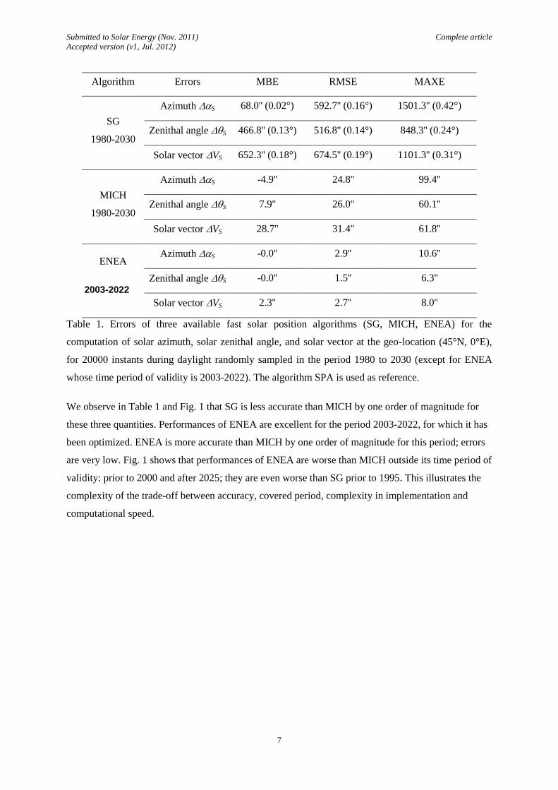
Table 1. Errors of three available fast solar position algorithms (SG, MICH, ENEA) for the
computation of solar azimuth, solar zenithal angle, and solar vector at the geo-location (45°N, 0°E),
for 20000 instants during daylight randomly sampled in the period 1980 to 2030 (except for ENEA
whose time period of validity is 2003-2022). The algorithm SPA is used as reference.
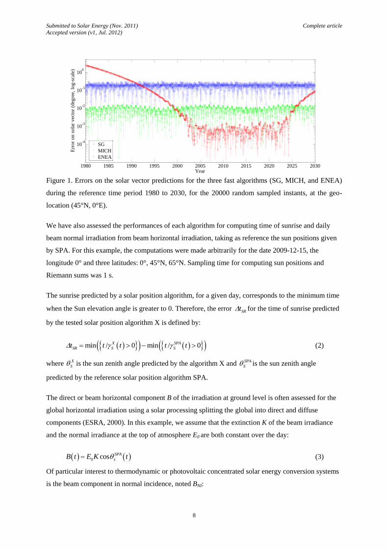
We observe in Table 1 and Fig. 1 that SG is less accurate than MICH by one order of magnitude for
these three quantities. Performances of ENEA are excellent for the period 2003-2022, for which it has
been optimized. ENEA is more accurate than MICH by one order of magnitude for this period; errors
are very low. Fig. 1 shows that performances of ENEA are worse than MICH outside its time period of
validity: prior to 2000 and after 2025; they are even worse than SG prior to 1995. This illustrates the
complexity of the trade-off between accuracy, covered period, complexity in implementation and
computational speed.
Submitted to Solar Energy (Nov. 2011) Complete article
Accepted version (v1, Jul. 2012)
8
Figure 1. Errors on the solar vector predictions for the three fast algorithms (SG, MICH, and ENEA)
during the reference time period 1980 to 2030, for the 20000 random sampled instants, at the geo-
location (45°N, 0°E).
We have also assessed the performances of each algorithm for computing time of sunrise and daily
beam normal irradiation from beam horizontal irradiation, taking as reference the sun positions given
by SPA. For this example, the computations were made arbitrarily for the date 2009-12-15, the
longitude 0° and three latitudes: 0°, 45°N, 65°N. Sampling time for computing sun positions and
Riemann sums was 1 s.
The sunrise predicted by a solar position algorithm, for a given day, corresponds to the minimum time
when the Sun elevation angle is greater to 0. Therefore, the error SRt for the time of sunrise predicted
by the tested solar position algorithm X is defined by:
min / 0 min / 0X SPA
SR S St t t t t (2)
where X
S is the sun zenith angle predicted by the algorithm X and SPA
S is the sun zenith angle
predicted by the reference solar position algorithm SPA.
The direct or beam horizontal component B of the irradiation at ground level is often assessed for the
global horizontal irradiation using a solar processing splitting the global into direct and diffuse
components (ESRA, 2000). In this example, we assume that the extinction K of the beam irradiance
and the normal irradiance at the top of atmosphere E0 are both constant over the day:
0 cos SPA
sB t E K t (3)
Of particular interest to thermodynamic or photovoltaic concentrated solar energy conversion systems
is the beam component in normal incidence, noted BNI:
1980 1985 1990 1995 2000 2005 2010 2015 2020 2025 2030
10-4
10-3
10-2
10-1
100
Year
Err
or
on s
ola
r vec
tor
(deg
ree,
log-s
cale
)
SG
MICH
ENEA
Submitted to Solar Energy (Nov. 2011) Complete article
Accepted version (v1, Jul. 2012)
9
0 cos 0SPAs
NI tB t E K t
(4)
where C t is the indicator function for the condition C(t).
When using the solar position algorithm X, the beam normal irradiance from the beam component on
horizontal surface is actually computed as follows:
0 cos 0
cos
cos cosXs
SPA
SX
NI X X tS S
B t tB t E K t
t
(5)
The relative error NI in the daily beam normal irradiation is defined:
cos 0 cos 0
cos 0
X SPAS S
SPAS
X SPA
NI NI
NISPA
NI
B t dt B t dt
B t dt
(6)
where the integrals are computed with Riemann sums with a sampling period of 1 s.
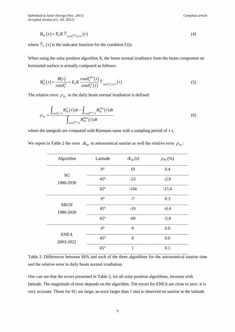
We report in Table 2 the error SRt in astronomical sunrise as well the relative error NI :
Algorithm Latitude SRt (s) NI (%)
SG
1980-2030
0° 19 0.4
45° -23 -2.0
65° -194 -15.6
MICH
1980-2030
0° -7 0.3
45° -19 -0.4
65° -69 -5.8
ENEA
2003-2022
0° 0 0.0
45° 0 0.0
65° 1 0.1
Table 2. Differences between SPA and each of the three algorithms for the astronomical sunrise time
and the relative error in daily beam normal irradiation.
One can see that the errors presented in Table 2, for all solar position algorithms, increase with
latitude. The magnitude of error depends on the algorithm. The errors for ENEA are close to zero: it is
very accurate. Those for SG are large; an error larger than 1 min is observed on sunrise at the latitude
Submitted to Solar Energy (Nov. 2011) Complete article
Accepted version (v1, Jul. 2012)
10
65°N. Furthermore, the relative error due only to the Sun position can amount up to 15.6 % in the case
of computation of beam normal irradiation from beam horizontal irradiation.
At latitude 65°N, MICH performs better than SG. Nevertheless, error in Sunrise may amount to 69 s.
Relative error can be greater than 5.8 % for computation of daily beam normal irradiation. The figures
indicated here are valid for the selected day only and are given for illustration; no conclusion should
be drawn for other days.
Table 2 demonstrates that an accurate assessment of the position of the Sun is needed for the accurate
assessment of the SSI. Together with Table 1, it also demonstrates that none of the proposed
algorithms meets our requirements. After having contemplated the extension or enhancement of the
three algorithms, we have opted for a new algorithm SG2, which is described now. The target for SG2
is the accuracy achieved by ENEA but extended to the period 1980-2030, instead of 2003-2022.
4. TIME SYSTEMS
Various time references should be considered. The International Atomic Time (TAI) is the basis of the
definition of the second, under the responsibility of the Bureau International des Poids et Mesures
(BIPM, www.bipm.org). The terrestrial time TT is equal to the TAI plus 32.184 s, and is the time scale
of ephemerides for Earth heliocentric position. The daily rotation of the Earth about itself determines
daytime and nighttime. A day is the time duration for one rotation; a day is divided into 24 h of 60 min
each as an average (mean solar day). The Universal Time (UT), also noted UT1, corresponds to a
fraction of the mean solar day; it is equal to 0 at midnight for longitude 0°. This time is not plainly
regular due to irregularities in Earth rotation (Markov et al., 2010; Mendes Cerveira et al., 2009). The
standard time is Coordinated Universal Time, abbreviated UTC. It is the basis of legal time and is
derived from International Atomic Time. The difference between UT and UTC is kept less than 1 s.
Therefore, the difference between UTC and TAI varies with the years and is under the responsibility
of the International Earth Rotation Service (McCarthy, Petit, 2003), which issues every June and
December a "Bulletin C'' message (ftp://hpiers.obspm.fr/iers/bul/bulc/bulletinc.dat), which reports the
introduction or not of a leap second, in order to guarantee |UT-UTC| < 1 s. Algorithms for Sun
position, including the one presented in this paper, usually require UT: to avoid small but systematic
angular errors related to the use of such algorithms in UTC time, one should refer to the "Bulletin D"
message at ftp://hpiers.obspm.fr/iers/bul/buld to get updated (bulltetind.dat) and previous (bulletind.*)
values of UT-UTC.
Of particular interest is the difference between the time TT and UT, TT:
TT = TT – UT (7)
Submitted to Solar Energy (Nov. 2011) Complete article
Accepted version (v1, Jul. 2012)
11
Values of TT are derived from observations only. The United States Naval Observatory (USNO)
provides monthly values of TT updated every 4 months, and a prediction of quarterly values for the
next seven years. The SPA also needs such values as an input parameter to correct for the Earth
irregular rotation (Reda and Andreas, 2004).
Analytical approximation of TT offers advantage in implementation and operation of the algorithm
and in prediction. Morrison and Stephenson (2004) proposed polynomial approximations for three
different periods: 1961-1986, 1986-2005, 2005-2050. Espenak and Meeus (2009) brought corrections
to these approximations. The last approximation was established in 2005 and has not yet been updated.
We propose to adopt these approximations whose piece-wise form per period permits to add new
approximations to the existing ones to account for measures and 9-year predictions of TT issued every
4 months by the USNO respectively at the web addresses http://maia.usno.navy.mil/ser7/deltat.data
and http://maia.usno.navy.mil/ser7/deltat.preds.
If y denotes the year, in integer form, e.g., 2010, and m the month ranging from 1 to 12, the year y in
decimal form is:
y = y + (m – 0.5)/12 (8)
We propose an approximation, notes TT-SG2:
5
1, 1
0
5
2, 2
0
3
2
3
, 3
0
if y 1980,1986
if y 1986,2005
if y 2005,2030
k
k
k
TT
k
k
k
k
k
k
TT SG
a y y
a y y
a y y
y
y (9)
The Table 3 provides the parameters yi and ai,k. These parameters are derived from Morrison and
Stephenson (2005) including modifications proposed by Espenak and Meerus (2009). Parameters of
the last third period 2005-2030 have been slightly modified to take into account USNO measurements
up to May 2012.
Submitted to Solar Energy (Nov. 2011) Complete article
Accepted version (v1, Jul. 2012)
12
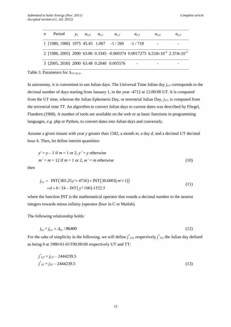
n Period yn an,0 an,1 an,2 an,3 an,4 an,5
1 [1980, 1986] 1975 45.45 1.067 -1 / 260 -1 / 718 - -
2 [1986, 2005] 2000 63.86 0.3345 -0.060374 0.0017275 6.51810-4
2.37410-5
3 [2005, 2030] 2000 63.48 0.2040 0.005576 - - -
Table 3. Parameters for TT-SG2.
In astronomy, it is convenient to use Julian days. The Universal Time Julian day jUT corresponds to the
decimal number of days starting from January 1, in the year -4712 at 12:00:00 UT. It is computed
from the UT time, whereas the Julian Ephemeris Day, or terrestrial Julian Day, jTT, is computed from
the terrestrial time TT. An algorithm to convert Julian days to current dates was described by Fliegel,
Flandern (1968). A number of tools are available on the web or as basic functions in programming
languages, e.g. php or Python, to convert dates into Julian days and conversely.
Assume a given instant with year y greater than 1582, a month m, a day d, and a decimal UT decimal
hour h. Then, let define interim quantities:
y' = y – 1 if m = 1 or 2, y’ = y otherwise
m’ = m + 12 if m = 1 or 2, m’ = m otherwise (10)
then
INT 365.25 ' 4716 INT 30.6001 ' 1
/ 24 – '/100 -1522.5
UTj y m
d h INT y
(11)
where the function INT is the mathematical operator that rounds a decimal number to the nearest
integers towards minus infinity (operator floor in C or Matlab).
The following relationship holds:
TT= / 86400TT UTj j (12)
For the sake of simplicity in the following, we will define j*
UT, respectively j*
TT, the Julian day defined
as being 0 at 1980-01-01T00:00:00 respectively UT and TT:
j*UT = jUT – 2444239.5
j*TT = jTT – 2444239.5 (13)
Submitted to Solar Energy (Nov. 2011) Complete article
Accepted version (v1, Jul. 2012)
13
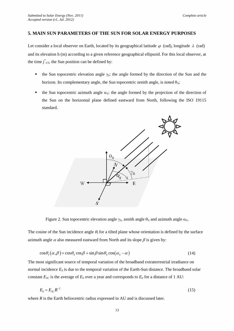
5. MAIN SUN PARAMETERS OF THE SUN FOR SOLAR ENERGY PURPOSES
Let consider a local observer on Earth, located by its geographical latitude (rad), longitude (rad)
and its elevation h (m) according to a given reference geographical ellipsoid. For this local observer, at
the time j*
UT, the Sun position can be defined by:
the Sun topocentric elevation angle S: the angle formed by the direction of the Sun and the
horizon. Its complementary angle, the Sun topocentric zenith angle, is noted S;
the Sun topocentric azimuth angle S: the angle formed by the projection of the direction of
the Sun on the horizontal plane defined eastward from North, following the ISO 19115
standard.
Figure 2. Sun topocentric elevation angle S, zenith angle S and azimuth angle S.
The cosine of the Sun incidence angle I for a tilted plane whose orientation is defined by the surface
azimuth angle also measured eastward from North and its slope is given by:
cos , cos cos sin sin cosI S S S (14)
The most significant source of temporal variation of the broadband extraterrestrial irradiance on
normal incidence E0 is due to the temporal variation of the Earth-Sun distance. The broadband solar
constant ESC is the average of E0 over a year and corresponds to E0 for a distance of 1 AU:
2
0 SCE E R (15)
where R is the Earth heliocentric radius expressed in AU and is discussed later.
Submitted to Solar Energy (Nov. 2011) Complete article
Accepted version (v1, Jul. 2012)
14
The value of the broadband solar constant Esc is set to 1367 W/m2: the typical day-to-day relative
variations of ESC due to solar activity are less than 0.15% and are considered negligible in the field of
solar energy (Schatten and Orosz, 1990; Wald, 2007).
These Sun parameters S, S, S, cosI and E0 are commonly used for solar energy studies as they
enable for example the computations of the extraterrestrial surface solar irradiance on a tilted plan, the
sunrise and sunset times or the shadow effects due to local horizon.
Submitted to Solar Energy (Nov. 2011) Complete article
Accepted version (v1, Jul. 2012)
15
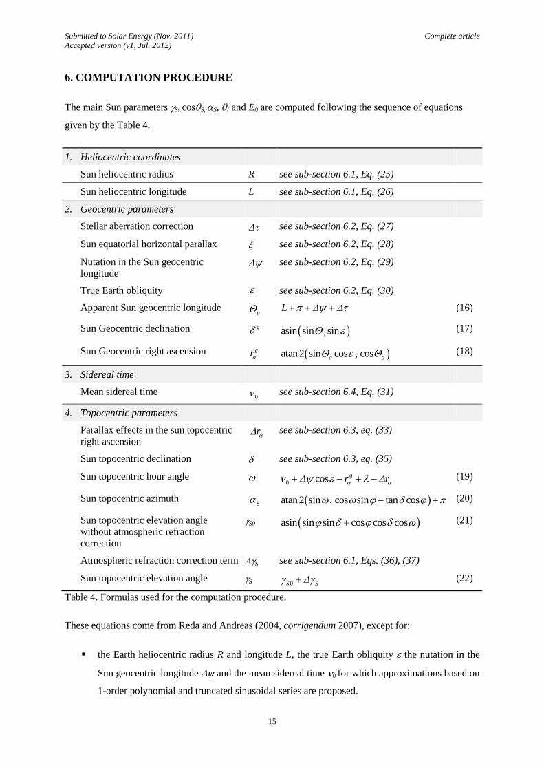
6. COMPUTATION PROCEDURE
The main Sun parameters S, cosS, S, I and E0 are computed following the sequence of equations
given by the Table 4.
1. Heliocentric coordinates
Sun heliocentric radius R see sub-section 6.1, Eq. (25)
Sun heliocentric longitude L see sub-section 6.1, Eq. (26)
2. Geocentric parameters
Stellar aberration correction
see sub-section 6.2, Eq. (27)
Sun equatorial horizontal parallax see sub-section 6.2, Eq. (28)
Nutation in the Sun geocentric
longitude
see sub-section 6.2, Eq. (29)
True Earth obliquity see sub-section 6.2, Eq. (30)
Apparent Sun geocentric longitude a
L
(16)
Sun Geocentric declination g asin sin sina (17)
Sun Geocentric right ascension gr atan 2 sin cos , cosa a
(18)
3. Sidereal time
Mean sidereal time 0 see sub-section 6.4, Eq. (31)
4. Topocentric parameters
Parallax effects in the sun topocentric
right ascension r see sub-section 6.3, eq. (33)
Sun topocentric declination see sub-section 6.3, eq. (35)
Sun topocentric hour angle 0 cos gr r
(19)
Sun topocentric azimuth S
atan2 sin , cos sin tan cos
(20)
Sun topocentric elevation angle
without atmospheric refraction
correction
S0 asin sin sin cos cos cos (21)
Atmospheric refraction correction term S see sub-section 6.1, Eqs. (36), (37)
Sun topocentric elevation angle S 0S S (22)
Table 4. Formulas used for the computation procedure.
These equations come from Reda and Andreas (2004, corrigendum 2007), except for:
the Earth heliocentric radius R and longitude L, the true Earth obliquity the nutation in the
Sun geocentric longitude and the mean sidereal time 0 for which approximations based on
1-order polynomial and truncated sinusoidal series are proposed.
Submitted to Solar Energy (Nov. 2011) Complete article
Accepted version (v1, Jul. 2012)
16
the Sun equatorial horizontal parallax and the stellar aberration correction for which
constant values are proposed ;
the parallax effects in the sun topocentric right ascension r and Sun topocentric
declination for which approximations based on simple 1-order Taylor expansion are
proposed ;
the atmospheric refraction correction s for which we propose to use an extended version for
low negative Sun topocentric elevation angle ;
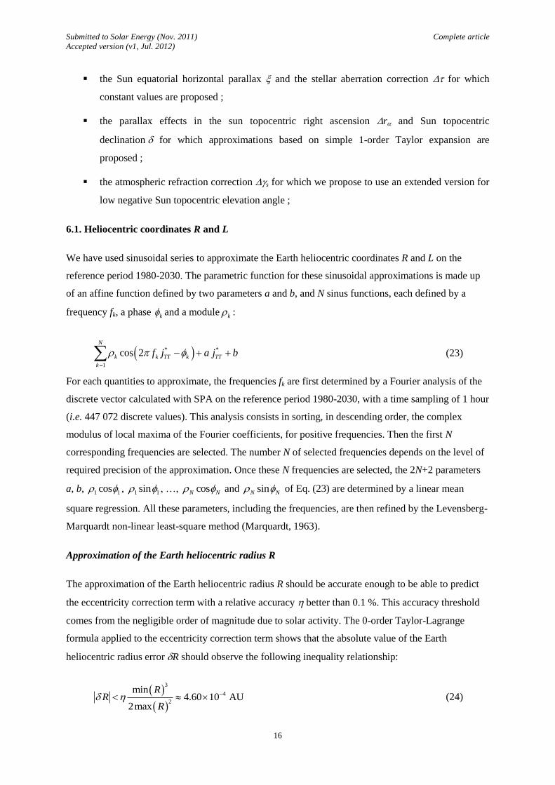
6.1. Heliocentric coordinates R and L
We have used sinusoidal series to approximate the Earth heliocentric coordinates R and L on the
reference period 1980-2030. The parametric function for these sinusoidal approximations is made up
of an affine function defined by two parameters a and b, and N sinus functions, each defined by a
frequency fk, a phase k and a module k :
* *
1
cos 2N
k k TT k TT
k
f j a j b
(23)
For each quantities to approximate, the frequencies fk are first determined by a Fourier analysis of the
discrete vector calculated with SPA on the reference period 1980-2030, with a time sampling of 1 hour
(i.e. 447 072 discrete values). This analysis consists in sorting, in descending order, the complex
modulus of local maxima of the Fourier coefficients, for positive frequencies. Then the first N
corresponding frequencies are selected. The number N of selected frequencies depends on the level of
required precision of the approximation. Once these N frequencies are selected, the 2N+2 parameters
a, b, 1 1cos , 1 1sin , …, cosN N and sinN N of Eq. (23) are determined by a linear mean
square regression. All these parameters, including the frequencies, are then refined by the Levensberg-
Marquardt non-linear least-square method (Marquardt, 1963).
Approximation of the Earth heliocentric radius R
The approximation of the Earth heliocentric radius R should be accurate enough to be able to predict
the eccentricity correction term with a relative accuracy better than 0.1 %. This accuracy threshold
comes from the negligible order of magnitude due to solar activity. The 0-order Taylor-Lagrange
formula applied to the eccentricity correction term shows that the absolute value of the Earth
heliocentric radius error R should observe the following inequality relationship:
3
4
2
min4.60 10 AU
2max
RR
R (24)
Submitted to Solar Energy (Nov. 2011) Complete article
Accepted version (v1, Jul. 2012)
17
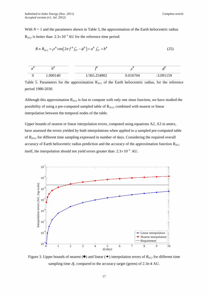
With N = 1 and the parameters shown in Table 5, the approximation of the Earth heliocentric radius
RSG2 is better than 42.3 10 AU for the reference time period:
* *
2 cos 2R R R R R
SG TT TTR R f j a j b (25)
aR b
R f
R ρ
R R
0 1.000140 1/365.254902 0.016704 -3.091159
Table 5. Parameters for the approximation RSG2 of the Earth heliocentric radius, for the reference
period 1980-2030.
Although this approximation RSG2 is fast to compute with only one sinus function, we have studied the
possibility of using a pre-computed sampled table of RSG2, combined with nearest or linear
interpolation between the temporal nodes of the table.
Upper bounds of nearest or linear interpolation errors, computed using equations A2, A3 in annex,
have assessed the errors yielded by both interpolations when applied to a sampled pre-computed table
of RSG2, for different time sampling expressed in number of days. Considering the required overall
accuracy of Earth heliocentric radius prediction and the accuracy of the approximation function RSG2
itself, the interpolation should not yield errors greater than 42.3 10 AU.
Figure 3. Upper bounds of nearest () and linear () interpolation errors of RSG2 for different time
sampling time j, compared to the accuracy target (green) of 2.3e-4 AU.
0 1 2 3 4 5 6 7 8 9 1010
-9
10-8
10-7
10-6
10-5
10-4
10-3
10-2
j (day)
Inte
rpo
lati
on
err
ors
(A
U,
log
-sca
le)
Linear interpolation
Nearest interpolation
Requirement
Submitted to Solar Energy (Nov. 2011) Complete article
Accepted version (v1, Jul. 2012)
18
Fig. 3 depicts the upper bounds of nearest and linear interpolation errors of RSG2 for different time
sampling. Linear interpolation always fits the accuracy requirement even with a pre-computed table of
RSG2 sampled every 10 days. As for the nearest interpolation, at least to a daily pre-computed table
should be sampled to fit the accuracy requirement.
Nearest interpolation applied on daily pre-computed table of RSG2 has been finally chosen for SG2, as
it requires only 2 floating operations per interpolation request, instead of 7 floating operations for the
linear interpolation.
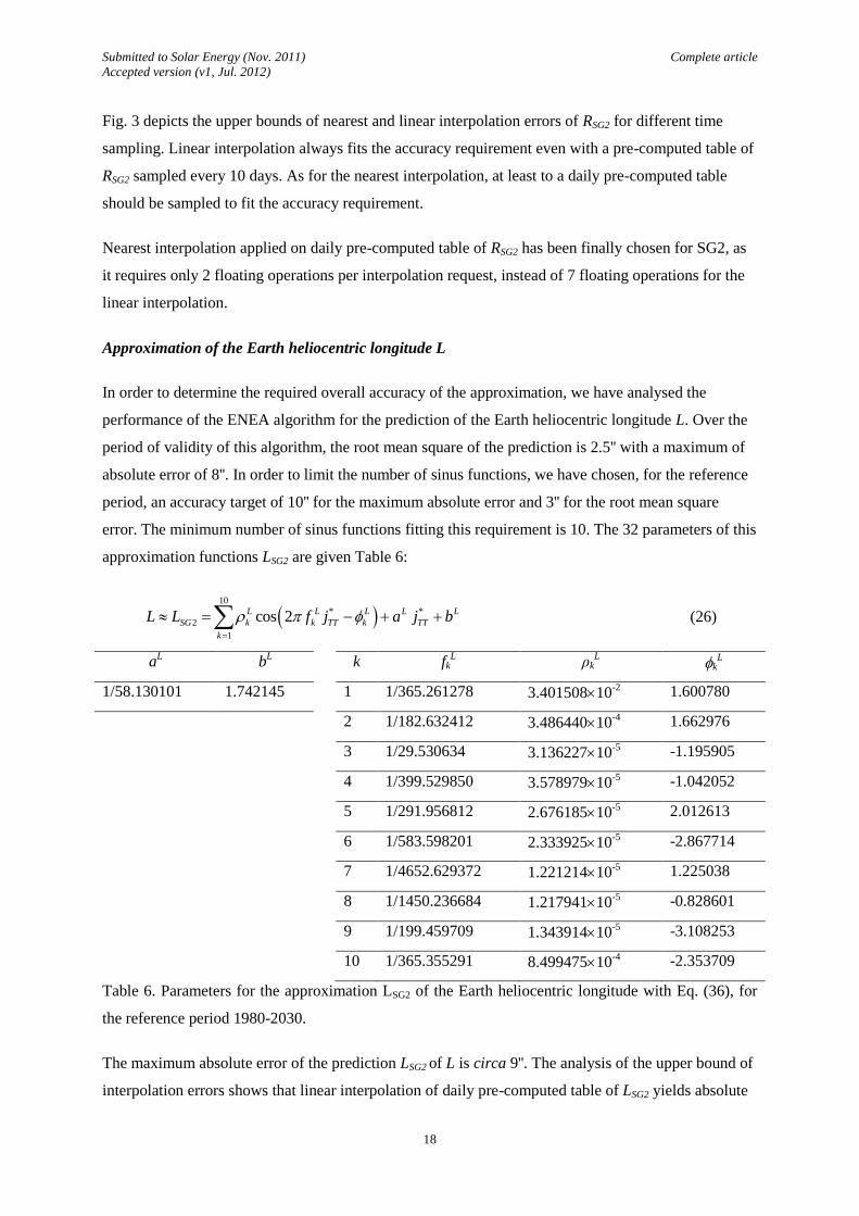
Approximation of the Earth heliocentric longitude L
In order to determine the required overall accuracy of the approximation, we have analysed the
performance of the ENEA algorithm for the prediction of the Earth heliocentric longitude L. Over the
period of validity of this algorithm, the root mean square of the prediction is 2.5'' with a maximum of
absolute error of 8''. In order to limit the number of sinus functions, we have chosen, for the reference
period, an accuracy target of 10'' for the maximum absolute error and 3'' for the root mean square
error. The minimum number of sinus functions fitting this requirement is 10. The 32 parameters of this
approximation functions LSG2 are given Table 6:
10
* *
2
1
cos 2L L L L L
SG k k TT k TT
k
L L f j a j b
(26)
aL b
L k fk
L ρk
L k
L
1/58.130101 1.742145 1 1/365.261278 3.40150810-2
1.600780
2 1/182.632412 3.48644010-4
1.662976
3 1/29.530634 3.13622710-5
-1.195905
4 1/399.529850 3.57897910-5
-1.042052
5 1/291.956812 2.67618510-5
2.012613
6 1/583.598201 2.33392510-5
-2.867714
7 1/4652.629372 1.22121410-5
1.225038
8 1/1450.236684 1.21794110-5
-0.828601
9 1/199.459709 1.34391410-5
-3.108253
10 1/365.355291 8.49947510-4
-2.353709
Table 6. Parameters for the approximation LSG2 of the Earth heliocentric longitude with Eq. (36), for
the reference period 1980-2030.
The maximum absolute error of the prediction LSG2 of L is circa 9''. The analysis of the upper bound of
interpolation errors shows that linear interpolation of daily pre-computed table of LSG2 yields absolute
Submitted to Solar Energy (Nov. 2011) Complete article
Accepted version (v1, Jul. 2012)
19
errors less than 1''. Therefore, linear interpolation applied on daily pre-computed table of LSG2 has been
finally chosen for the Earth heliocentric longitude in SG2.
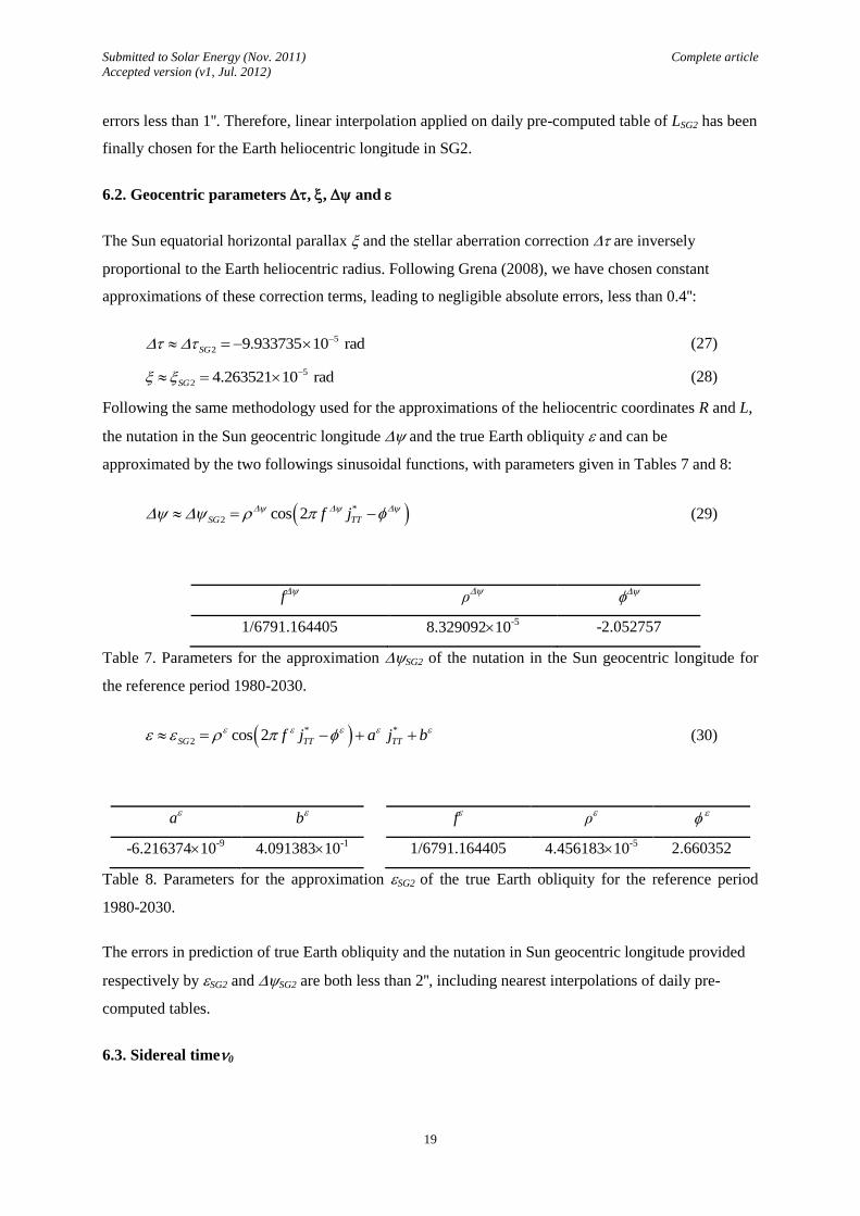
6.2. Geocentric parameters , , and
The Sun equatorial horizontal parallax and the stellar aberration correction are inversely
proportional to the Earth heliocentric radius. Following Grena (2008), we have chosen constant
approximations of these correction terms, leading to negligible absolute errors, less than 0.4'':
5
2 9.933735 10 radSG (27)
5
2 4.263521 10 radSG (28)
Following the same methodology used for the approximations of the heliocentric coordinates R and L,
the nutation in the Sun geocentric longitude and the true Earth obliquity and can be
approximated by the two followings sinusoidal functions, with parameters given in Tables 7 and 8:
*
2 cos 2SG TTf j (29)
f
ρ
1/6791.164405 8.32909210-5
-2.052757
Table 7. Parameters for the approximation SG2 of the nutation in the Sun geocentric longitude for
the reference period 1980-2030.
* *
2 cos 2SG TT TTf j a j b (30)
a b
f
ρ
-6.21637410-9
4.09138310-1
1/6791.164405 4.45618310-5
2.660352
Table 8. Parameters for the approximation SG2 of the true Earth obliquity for the reference period
1980-2030.
The errors in prediction of true Earth obliquity and the nutation in Sun geocentric longitude provided
respectively by SG2 and SG2 are both less than 2'', including nearest interpolations of daily pre-
computed tables.
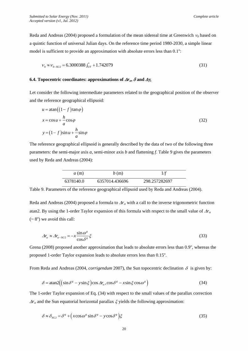
6.3. Sidereal time0
Submitted to Solar Energy (Nov. 2011) Complete article
Accepted version (v1, Jul. 2012)
20
Reda and Andreas (2004) proposed a formulation of the mean sidereal time at Greenwich 0 based on
a quintic function of universal Julian days. On the reference time period 1980-2030, a simple linear
model is sufficient to provide an approximation with absolute errors less than 0.1'':
*
0 0 2 6.3000388 1.742079SG UTj
(31)
6.4. Topocentric coordinates: approximations of r, and s
Let consider the following intermediate parameters related to the geographical position of the observer
and the reference geographical ellipsoid:
atan 1 tan
cos cos
1 sin sin
u f
hx u
a
hy f u
a
(32)
The reference geographical ellipsoid is generally described by the data of two of the following three
parameters: the semi-major axis a, semi-minor axis b and flattening f. Table 9 gives the parameters
used by Reda and Andreas (2004):
a (m) b (m) 1/f
6378140.0 6357014.436696 298.257282697
Table 9. Parameters of the reference geographical ellipsoid used by Reda and Andreas (2004).
Reda and Andreas (2004) proposed a formula to r with a call to the inverse trigonometric function
atan2. By using the 1-order Taylor expansion of this formula with respect to the small value of r
(~ 8'') we avoid this call:
2
sin
cos
g
SG gr r x
(33)
Grena (2008) proposed another approximation that leads to absolute errors less than 0.9'', whereas the
proposed 1-order Taylor expansion leads to absolute errors less than 0.15''.
From Reda and Andreas (2004, corrigendum 2007), the Sun topocentric declination is given by:
atan2 sin sin cos ,cos sin cosg g gy r x (34)
The 1-order Taylor expansion of Eq. (34) with respect to the small values of the parallax correction
r and the Sun equatorial horizontal parallax yields the following approximation:
2 cos sin cosg g g g
SG x y (35)
Submitted to Solar Energy (Nov. 2011) Complete article
Accepted version (v1, Jul. 2012)
21
As for the parallax effects in the sun topocentric right ascension, Grena (2008) proposed another
approximation that exhibits absolute errors less than 2.8'' whereas this 1-order Taylor expansion yields
absolute errors less than 0.15'', with the same order of computational complexity.
Reda and Andreas (2004) use the atmospheric refraction correction term of Meeus (1999), taking into
account the yearly average local air pressure P expressed in hPa, the yearly average of local air
temperature T expressed in °C and the Sun topocentric elevation angle.
This correction, valid for S0 greater than -0.01 rad, is
S0 0.01
4
2 1
0 0
283 2.96706 10
1010 273 tan 0.0031376 0.089186S S SG
S S
P
T
(36)
For S0 less than -0.01 rad, we use the correction term of Cornwall et al. (2011):
2
S0 0.01
4
0
283 1.005516 10
1010 273 tanS SGS
S
P
T
(37)
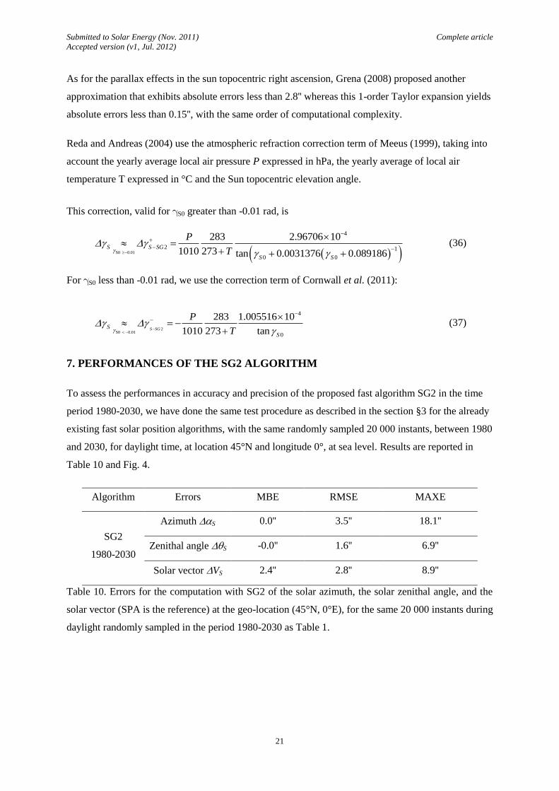
7. PERFORMANCES OF THE SG2 ALGORITHM
To assess the performances in accuracy and precision of the proposed fast algorithm SG2 in the time
period 1980-2030, we have done the same test procedure as described in the section §3 for the already
existing fast solar position algorithms, with the same randomly sampled 20 000 instants, between 1980
and 2030, for daylight time, at location 45°N and longitude 0°, at sea level. Results are reported in
Table 10 and Fig. 4.
Algorithm Errors MBE RMSE MAXE
SG2
1980-2030
Azimuth S 0.0'' 3.5'' 18.1''
Zenithal angle S -0.0'' 1.6'' 6.9''
Solar vector VS 2.4'' 2.8'' 8.9''
Table 10. Errors for the computation with SG2 of the solar azimuth, the solar zenithal angle, and the
solar vector (SPA is the reference) at the geo-location (45°N, 0°E), for the same 20 000 instants during
daylight randomly sampled in the period 1980-2030 as Table 1.
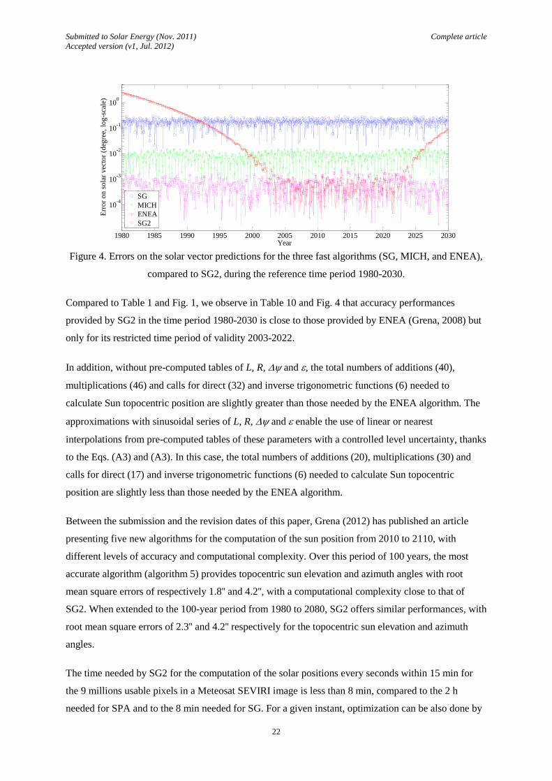
Submitted to Solar Energy (Nov. 2011) Complete article
Accepted version (v1, Jul. 2012)
22
Figure 4. Errors on the solar vector predictions for the three fast algorithms (SG, MICH, and ENEA),
compared to SG2, during the reference time period 1980-2030.
Compared to Table 1 and Fig. 1, we observe in Table 10 and Fig. 4 that accuracy performances
provided by SG2 in the time period 1980-2030 is close to those provided by ENEA (Grena, 2008) but
only for its restricted time period of validity 2003-2022.
In addition, without pre-computed tables of L, R, and , the total numbers of additions (40),
multiplications (46) and calls for direct (32) and inverse trigonometric functions (6) needed to
calculate Sun topocentric position are slightly greater than those needed by the ENEA algorithm. The
approximations with sinusoidal series of L, R, and enable the use of linear or nearest
interpolations from pre-computed tables of these parameters with a controlled level uncertainty, thanks
to the Eqs. (A3) and (A3). In this case, the total numbers of additions (20), multiplications (30) and
calls for direct (17) and inverse trigonometric functions (6) needed to calculate Sun topocentric
position are slightly less than those needed by the ENEA algorithm.
Between the submission and the revision dates of this paper, Grena (2012) has published an article
presenting five new algorithms for the computation of the sun position from 2010 to 2110, with
different levels of accuracy and computational complexity. Over this period of 100 years, the most
accurate algorithm (algorithm 5) provides topocentric sun elevation and azimuth angles with root
mean square errors of respectively 1.8'' and 4.2'', with a computational complexity close to that of
SG2. When extended to the 100-year period from 1980 to 2080, SG2 offers similar performances, with
root mean square errors of 2.3'' and 4.2'' respectively for the topocentric sun elevation and azimuth
angles.
The time needed by SG2 for the computation of the solar positions every seconds within 15 min for
the 9 millions usable pixels in a Meteosat SEVIRI image is less than 8 min, compared to the 2 h
needed for SPA and to the 8 min needed for SG. For a given instant, optimization can be also done by
1980 1985 1990 1995 2000 2005 2010 2015 2020 2025 2030
10-4
10-3
10-2
10-1
100
Year
Err
or
on s
ola
r vec
tor
(deg
ree,
log-s
cale
)
SG
MICH
ENEA
SG2
Submitted to Solar Energy (Nov. 2011) Complete article
Accepted version (v1, Jul. 2012)
23
pre-computing tables for quantities not depending on the geographical coordinates, such as the sun
geocentric positions.
8. CONCLUSION
The present article proposes a new algorithm SG2 which is fast and accurate: over the period 1980-
2030, the maximum error in the solar vector is less than 0.0025° (~ 9'') and the uncertainty of the Sun
topocentric azimuth and elevation is c. 0.0015° (~ 5''). It is accurate enough for calibration of
pyranometers and pointing devices (Reda and Andreas, 2003, 2004; Stafford et al., 2009). It is fast
enough for its use in the HelioClim processing and post-processing chains and other similar
computational chains. It is accurate enough so that the influence of the Sun position on the error
budget of satellite-derived assessment of SSI is of second-order or negligible.
Several approximations are made of the original equations of the SPA to decrease the number of
operations. These approximations result in a decrease of accuracy compared to SPA and we have
presented the mathematical tools permitting to determine these approximations with a selected
uncertainty level. These tools will permit further development of other algorithms meeting other
requirements than HelioClim. Like the ESRA algorithm, software libraries in C and Matlab are
available on the Web (www.helioclim.org) and should help such developments. A Web service is also
available at www.webservice-energy.org. It is an application that can be invoked via the Web. It could
be used to check the correctness of implementation of the SG2 algorithm or can be used for the
computation of the Sun position.
ANNEX A – COMPUTATION OF UPPER BOUND OF ERROR IN
INTERPOLATING A DISCRETE SINUSOIDAL SERIES
Let consider a function s(t) defined by a truncated Fourier series and an affine function:
1
cos 2N
k k k
k
s t f t t
(A1)
st is a discrete signal resulting from the sampling of s(t) with a sampling period t, and an arbitrary
sampling phase t0:
0ts k s k t t (A2)
The upper bounds of error when interpolating the discrete signal st by the nearest neighbor and linear
interpolations are respectively noted UBN and UBL, and are given:
Submitted to Solar Energy (Nov. 2011) Complete article
Accepted version (v1, Jul. 2012)
24
1
2
N
N k k
k
UB f t
(A3)
2 2 2
1
4N
L k k
k
UB t f
(A4)
ACKNOWLEDGMENTS
The research leading to these results has received funding from the European Union’s Seventh
Framework Programme (FP7/2007-2013) under Grant Agreement no. 262892 (ENDORSE project).
Submitted to Solar Energy (Nov. 2011) Complete article
Accepted version (v1, Jul. 2012)
25
REFERENCES
Blanc, Ph., Gschwind, B., Lefèvre, M., Wald, L., 2011. The HelioClim project: surface solar
irradiance data for climate application. Remote Sensing, in press, 3(2), 343-361,
doi:10.3390/rs20x000x
Blanco-Muriel, M., Alarcón-Padilla, D. C., López-Moratalla, T., Lara-Coira, M., 2001. Computing the
solar vector. Solar Energy, 70(5), 431-441.
Bretagnon, P., Francou, G., 1988. Planetary theories in rectangular and spherical variables. VSOP87
solutions. Astronomy & Astrophysics, 202, 309-315.
Cornwall, C., Horiuchi, A., Lehman, C. 2011. Solar calculator. NOAA Earth System Research Lab.
http://www.srrb.noaa.gov/highlights/sunrise/azel.html, last accessed: May 2011.
Cros, S., Albuisson, M., Lefèvre, M., Rigollier, C., Wald, L., 2004. HelioClim: a long-term database
on solar radiation for Europe and Africa. In Proceedings of EuroSun 2004, published by PSE GmbH,
Freiburg, Germany, pp. (3)916-920.
Diabaté, L., Moussu, G., Wald, L., 1989. Description of an operational tool for determining global
solar radiation at ground using geostationary satellite images. Solar Energy, 42(3), 201-207.
Espenak, F., Meeus, J., 2009. Five millennium catalog of solar eclipses: –1999 to +3000 (2000 bce to
3000 ce)—revised. Technical Report NASA/TP–2009–214174, NASA.
Espinar, B., Ramírez, L., Polo, J., Zarzalejo, L.F., Wald, L., 2009. Analysis of the influences of
uncertainties in input variables on the outcomes of the Heliosat-2 method. Solar Energy, 83, 1731-
1741, doi:10.1016/j.solener.2009.06.010
ESRA, 2000. European Solar Radiation Atlas. Fourth edition, includ. CD-ROM. Edited by Greif, J.,
and K. Scharmer. Scientific advisors: R. Dogniaux, J. K. Page. Authors: L. Wald, M. Albuisson, G.
Czeplak, B. Bourges, R. Aguiar, H. Lund, A. Joukoff, U. Terzenbach, H. G. Beyer, E. P. Borisenko.
Published for the Commission of the European Communities by Presses de l'Ecole, Ecole des Mines
de Paris, Paris, France.
Fliegel, H. F., Flandern, T. C. V., 1968. A machine algorithm for processing calendar dates.
Communications of the ACM, 11(10), 657.
Grena, R., 2008. An algorithm for the computation of the solar position. Solar Energy, 82(5), 462-470,
doi:10.1016/j.solener.2007.10.001.
R. Grena, 2012. Five new algorithms for the computation of sun position from 2010 to 2110, Solar
Energy, vol. 86(5), 1323-1337, doi:10.1016/j.solener.2012.01.024.
Submitted to Solar Energy (Nov. 2011) Complete article
Accepted version (v1, Jul. 2012)
26
Gschwind, B., Ménard, L., Albuisson, M., Wald, L., 2006. Converting a successful research project
into a sustainable service: the case of the SoDa Web service. Environmental Modelling and Software,
21, 1555-1561, doi:10.1016/j.envsoft.2006.05.002.
ISO 19115, 2003. Geographic information – Metadata. Correction 2006. International Organization
for Standardization. Geneva, Switzerland.
Kambezidis, H. D., Tsangrassoulis, A. E., 1993. Solar position and right ascension. Solar Energy,
50(5), 415-416.
Lefèvre, M., Diabaté, L., Wald, L., 2007. Using reduced data sets ISCCP-B2 from the Meteosat
satellites to assess surface solar irradiance. Solar Energy, 81, 240-253,
doi:10.1016/j.solener.2006.03.008.
Markov, Y. G., Perepelkin, V. V., Sinitsyn, I. N., Semendyaev, N. N., 2010. Rotational-oscillatory
motion of the Earth and the global component of the seismic process. Doklady Physics, 55(11), 583-
587, doi: 10.1134/S1028335810110121.
McCarthy, D. D., Petit, G., 2003. IERS conventions (2003). IERS Technical Note 32, International
Earth Rotation and Reference System Service. Verlag des Bundesamts für Kartographie und Geodäsie,
Frankfurt am Main, Germany, 2004. 127 pp.
Marquardt, D., 1963. An algorithm for least-squares estimation of nonlinear parameters, SIAM
Journal Applied Math., 11, 431–441.
Meeus, J., 1999. Astronomical Algorithms (2nd
edition). Willmann-Bell Inc., Richmond, Va, USA,
477 pp.
Mendes Cerveira, P. J., Boehm, J., Schuh, H., Kluegel, T., Velikoseltsev, A., Schreiber, K. U.,
Brzezinski, A., 2009. Earth rotation observed by very long baseline interferometry and ring laser. Pure
and Applied Geophysics, 166(8-9), 1499-1517, doi: 10.1007/s00024-004-0487-z.
Michalsky, J., 1988. The astronomical almanac's algorithm for approximate solar position (1950–
2050). Solar Energy, 40(3), 227-235.
Morrison, L., Stephenson, F. R., 2004. Historical values of the Earth's clock error Delta T and the
calculation of eclipses. Journal for the History of Astronomy, 35(120), 327–336.
Perez, R., Ineichen, P., Moore, K., Kmiecik, M., Chain, C., George, R., Vignola, F., 2002. A new
operational model for satellite-derived irradiances: description and validation. Solar Energy, 73(5),
307-317, doi: 10.1016/S0038-092X(02)00122-6.
Pitman, C.L., Vant-Hull, L.L., 1978. Errors in locating the Sun and their effect on solar intensity
predictions. In: Meeting of the American Section of the International Solar Energy Society, Denver,
28 August 1978, pp. 701–706.
Submitted to Solar Energy (Nov. 2011) Complete article
Accepted version (v1, Jul. 2012)
27
Reda, I., Andreas, A., 2003. Solar position algorithm for solar radiation applications: Technical
Report, National Renewable Energy Laboratory, Golden, Co, USA. Revised version: January 2008.
Reda, I., Andreas, A., 2004. Solar position algorithm for solar radiation applications: Solar Energy,
76(5), 577–589. Corrigendum, 81, 838-838, 2007.
Rigollier, C., Lefèvre, M., Wald, L., 2004. The method Heliosat-2 for deriving shortwave solar
radiation from satellite images. Solar Energy, 77(2), 159-169.
Stafford, B., Davis, M., Chambers, J., Martínez, M., Sanchez, D., 2009. Tracker accuracy: field
experience, analysis, and correlation with meteorological conditions. In Proceedings of the 34th IEEE
Photovoltaic Specialists Conference, Philadelphia, USA, June 7-12, 2009, pp. 2256-2259.
Schatten, K. H., Orosz, J. A., 1990. Solar constant secular changes. Solar physics, 125, 179-184,
doi:10.1007/BF00154787.
Wald, L., 2007. Solar radiation energy (fundamentals). In Solar Energy Conversion and Photoenergy
Systems, edited by Julian Blanco and Sixto Malato, in Encyclopedia of Life Support Systems
(EOLSS), Developed under the Auspices of the UNESCO, Eolss Publishers, Oxford ,UK,
[http://www.eolss.net]
Walraven, R., 1978. Calculating the position of the Sun. Solar Energy, 20, 393-397.