THE SENSITIVITY OF EVAPORATION RATE TO CLIMATE CHANGE-

RESULTS OF AN ENERGY-BALANCE APPROACH

By Larry Benson

U.S. GEOLOGICAL SURVEY

Water-Resources Investigations Report 86-4148

Denver, Colorado 1986

UNITED STATES DEPARTMENT OF THE INTERIOR

DONALD PAUL HODEL, Secretary

GEOLOGICAL SURVEY

Dallas L. Peck, Director

For additional information write to:

L. Benson, Project Chief U.S. Geological Survey Box 25046, Mail Stop 403 Denver Federal Center Denver, CO 80225

Telephone: (303) 236-5917

For sale by:

Open-File Services Section Western Distribution Branch U.S. Geological Survey Box 25425, Mail Stop 306 Denver Federal Center Denver, CO 80225

Telephone: (303) 236-7476

CONTENTS

Page Symbols, variables, dimensions, and definitions used in equations andEVAP computer program------------ ---------------- __________________ v

Abstract--------------- ---------------------------- _________ _______ iIntroduction---- _________________ ___ ___________ __________________ ±

Changes in the surface altitudes of Great Basin lakes---------- --- 1Change in the size of lakes in the Lahontan basin, 12,500 to

12,000 years before present--------------- -- -----__________-__ 4Methods for the calculation of evaporation rate-------- - _____________ 10

Covariance methods--------------- ---- _________ ________________ IQAerodynamic (mass-transfer) method-- ------ --- - -------------- 12The Dalton concept--------------------- --------- ________________ 12Energy-balance method----------------------------------------------- 13Combination methods------------------------------------- ---- ---- 14Empirical methods-------------------------------------------------- 16Comparison of methods and choice of energy-balance method for the

calculation of evaporation rate for use in sensitivity analyses--- 18 Theoretical and empirical formulae used in the energy-balance method----- 19

Solar radiation--------------- --------------------------------- - 19Short-wave radiation--------- -- ------------ ___________________ 20Long-wave radiation- ____________________________________ _ ____ 21

Sensitivity analysis--------------------------------- ----- ----------- 24Parameter variation----------------------------- ------------------ 32Parameter combinations-------- -------------------------- ________ 34Results of sensitivity analysis-------- -- -- -------------- --- 35

Possible causes of evaporation-rate reduction in the Lahontan basin14,000 to 12,500 years ago 35

Air temperature-------------- ---------------------------- _______ 37Cloud cover------------------------------------- ----- ----------- 37Water temperature--- -------------------------- __-__ _________ 37

Summary and conclusions-- ___-____________________________-------------- 37References------- ------ ________--_-- _______________________________ 33

FIGURES

Page Figure 1. Map showing Late Pleistocene lakes of the Great Basin--------- 2

2. Graph showing fluctuations in lake-surface altitudes for LakeRussell, Lake Lahontan, and Lake Bonneville----------------- 3

3. Map showing surface area of Lake Lahontan 14,000 to 12,500 years before present and location of subbasins and sills separating subbasins---------------------------------------- 5

4. Map showing location of streamflow-gaging and weather stationsfor which data are available for 1969----------------------- 7

5. Graph showing mean annual discharge for the Carson (1942-82),Truckee (1942-82), and Walker (1958-77) Rivers 8

6. Map showing hypothetical surface areas of lakes in theLahontan basin if the runoff and precipitation that occurredin 1969 became the mean----------------- -______------- -- n

111

Figures 7-9

Table 1

2

345

8

Graphs showing:7. Relation of evaporation and

United States---- Deviations of solar

at 40° north latitude Evaporation rate as

(Q-0; B, relativetype fraction ofof medium-level cloudslevel clouds (f-i-iE, increase in tri

irradiation from their 1950 values

function of: A, solar radiation umidity (RH); C, cloud-cover

high-level clouds (f,,), fraction(f ,), and fraction of low-

; D, amount of sky cover (x); and

(T ) and water a temperature

TABLES

Streamflow statistics Lahontan basin- -----

Precipitation statistics the floor of the Lahon

Reference-climate dataEVAP computer program liComputed evaporation rat

tions of cloud type, combinations of air relative humidity---

Solar irradiation for th latitude for 1950, 12, 18,000 years before pr

Values of parameters used analys i s---------

for rivers that discharge to the

temperature in the western

Page

17

19

difference between air temperature36

for weather stations located on tan basin, California and Nevada--- et for Pyramid Lake, Nevada----- -sting--p---------------------------IBS, in meters per year, for frac-

ainount of sky cover, and various temperature, water temperature, and

e 21st of each month at 40° north 300 yeatrs before present, and esent-in evaporation-sensitivity

Page

92526

31

33

34

IV

A. J

hi

11

ml

hi

11

'ml

hi

11

ml

m

w

SYMBOLS, VARIABLES, DIMENSIONS, AND DEFINITIONS USED IN EQUATIONS AND EVAP COMPUTER PROGRAM

- (cm2 ) area of the jth layer of water.

- ALBHI - (dimensionless) albedo of high-altitude cirrus clouds;

- (cm2 )

AU1 = 0.21. hi

area of lake.

- ALBLO - (dimensionless) albedo of low-level heap clouds;A = 0.70.

- ALBMED - (dimensionless) albedo of medium-altitude clouds;

"°' 19l6a

A , = 0.48. ml

AH

AL

AM

ALTHI

- (dimensionless) = 0. hl) .

- (dimensionless) a = 0. 74+f 1 ,(0.025xe~°' 19l6ofn) .

- (dimensionless) a ̂ = 0.74+f (0.025xe~°* 19l60 ml) .

- (dimensionless) altitude of high-level clouds;a, .. = 6 km. hi

- ALTLO - (dimensionless) altitude of low-level clouds;a = 1 km.

- ALTMED - (dimensionless) altitude of medium-level clouds;

~°* 1969a

a .. = 4 km. ml

BH

BL

BM

BOWRAT

- (dimensionless)

- (dimensionless)

= 0.00490-fhl (0.00054xe hl) .

= 0.00490-fn (0.00054xe~°* 1969an) .

- (dimensionless) b _ = 0.00490-f 1 (0.00054xe~°' 1969°ml) .ml ml

- (dimensionless) Bowen ratio; the ratio of the energy con­ducted to (or from) the air as sensible heat to energy used for evaporation (latent heat) .

- (dimensionless) bulk-vaporation coefficient.

- (dimensionless) mass-transfer coefficient.

- (cal g~ l °K~ 1 ) specific heat of water; C - 1.0.w

P d d" 1

- (cal g" 1 °K-1 OT/--I specific heat of air at constant pressure.

- (dimensionless) ratio of the mean Earth-sun distance to theinstantaneous distance; d d" 1 - 1.0.

do

dld2

d3

d4

d5

d6

D g

Dr

A

E

EV

E iE30

E365

e

e

- DO - (dimensionless) d_ =

- Dl - (dimensionless) d 1 =

- D2 - (dimensionless) d_ =

- D3 - (dimensionless) d~ =

- D4 - (dimensionless) d, =

- D5 - (dimensionless) d_ =

- D6 - (dimensionless) d,, = o

- (cm3 ) grou

- (cm3 ) runo

- (dimensionless) slop

- (cm yr" 1 ) evap

- (cm3 cm" 2 s" 1 ) eddy

- EVAP - (cm d" 1 ) dail

- MEVAP - (cm mo" 1 ) mont

- ANEVAP - (m yr" 1 ) annu

- (dimensionless) Napi

- (dimensionless) the

6984.5D5294.

-188.9039310.

2.13*3357675.

-1.288580973E-2.

4.393587233E-5.

-8.023923082E-8.

6.136820929E-11.

nd-water discharge into lake.

ff into lake.

e of saturation water-vapor curve.

oration rate.

-vapor flux.

y evaporation rate.

tily evaporation rate.

al evaporation rate.

erian logarithm base; e = 2.7183.

emissivity of water at water-surfa

'hi

11

ml

- MVP

- SVPOM

- SVP2M

- FRHI

- FRLO

- FRMED

(mb)

(mb)

(mb)

(dimensionless)

(dimensionless)

(dimensionless)

(dimensionless)

temperature, T ; e - 0.97.

vapor pressure of the air, for the actual condition of humidity.

ivapor pressure of saturated air at tempera­

ture. T . of the water surface.~ ' o'

vapor pressure of saturated air at the

cJ

cJ

ol served air temperature, T

fraction oi: sky covered by high-altitudeouds.

fraction of sky covered by low-altitudeouds.

fraction of sky covered by medium-altitude ci.ouds.

psychrometric constant.

Y* - (degrees) solar altitude, the angle of the sunabove the horizon.

L - LHEAT - (cal g" 1 ) latent heat of vaporization of water attemperature, T .

A. - (cal cm" 2 ) Langley; the energy unit of solar radia­ tion; A. = 1 cal cm" 2 .

M - MASSAIR - (dimensionless) mean optical air mass, the length of theatmospheric path traversed by the sun's rays in reaching the Earth, measured in terms of the length of this path when the sun is in the zenith.

P - P - (mb) atmospheric pressure at a standard distanceabove the water surface.

P, - (cm) precipitation that falls on lake.

Q* - QSTAR - (cal cm" 2 d" 1 ) solar irradiation incident on the upperatmosphere at a specified latitude.

Q - QA - (cal cm" 2 d" 1 ) long-wave radiation falling on the watersurface from the atmosphere.

Q , .. - QAH - (cal cm" 2 d" 1 ) long-wave radiation falling on the water ' surface from high-level clouds.

Q .... - QAL - (cal cm" 2 d" 1 ) long-wave radiation falling on the water ' surface from low-level clouds.

Q , - QAM - (cal cm" 2 d"" 1 ) long-wave radiation falling on the water ' surface from medium-level clouds.

Q - QAR - (cal cm" 2 d" 1 ) the part of the incoming long-wave radia­ tion that is reflected from the water surface back to the atmosphere.

Q. - QBS - (cal cm" 2 d" 1 ) long-wave radiation emitted by the body ofwater; the numerical value of Q, is determined by the surface temperature of the water.

Q - - (cal cm" 2 d" 1 ) energy flux resulting from a change in thelatent heat content of evaporating water.

Q, - (cal cm" 2 d" 1 ) energy flux conducted from the water as sen­ sible heat (enthalpy) during evaporation.

Q - QR - (cal cm" 2 d" 1 ) the part of the incoming solar radiationthat is reflected from the water surface.

VII

v

w

R

R

R

RH

QS

QV

- QNU

- HUMID

(cal cm 2 d *)

(cal cm" 2 d" 1 )

(cal)

(cal cm~ 2 d' 1 )

solar radiation incident to the water surface.

net thi

leat energy brought (advected) intoe body

ground-water sources and sinks.

net leat stored in body of water.

energy flux

(dimensionless)

(dimensionless) diff

(dimensionless)

(cal cm" 2 d" 1 )

(dimensionless)

(cal cm" 2 s" 1 )

(dimensionless)

(dimensionless)

(g cm" 3 )

(g cm" 3 )

(g cm" 3 )

(g cm" 3 )

of

long

of water by all surface- and

resulting from advection ofevaporating water,

specific humidity.

erence between turbulent fluctuation specific humidity and its mean valuein

saturation- specific humidity at water- surface temperature.

change in the energy stored in the bodywater.

-wave reflectivity of the watersurface; R - 0.030.^ ' a

netsurface.

solasurface;

rel, wa tosaturation.

air

dens

dens

- (cal cm" 2 min" 1 ) the

(cal cm" 2 d" 1 OR' 1 )

- (h)

radiative flux density reaching water

r-radiation reflectivity of the water

ter vap

R 0.07.

tive humidity; ratio of the actualor present in a parcel of air

that which would be present at

density.

ity of

ity of

density of

water undergoing evaporation,

jth layer of lake water,

advected surface and groundwa ter.

solar constant; S = 1.94.

Steiian's constant; a = 11.71X10" 8 .

duration of sunshine at a specific titude

V] 11

T - AIRT - (°K) temperature of the air at a standarddistance above the body of water.

T - BASET - (°K) arbitrary base temperature of the body ofwater; Tb = 273.15°K.

T. - (°K) mean temperature of ith source of advectedwater.

T. - (°K) mean temperature of jth layer of lake J water.

T - WATERT - (°K) surface temperature of the body of waterundergoing evaporation.

T, - DEWPT - (°K) dewpoint temperature, the temperature to P which a parcel of air must be cooled at

constant pressure and water-vapor content to achieve saturation.

T , - TAUALB - (dimensionless) atmospheric transmission coefficientresulting from cloud albedo.

T, - TAUDRY - (dimensionless) atmospheric transmission coefficient result­ ing from dry-air scattering.

T - TAUWET - (dimensionless) atmospheric transmission coefficient result­ ing from water-vapor absorption.

T - TAUSCAT - (dimensionless) atmospheric transmission coefficient result­ ing from water-vapor scattering.

u - - (cm s" 1 ) wind velocity.

V. - - (cm3 ) volume of water input to the lake from theith surface- or ground-water source.

W - WLOFT - (cm) precipitable water aloft, (that is, totalwater-vapor content of the air at all levels).

w' - - (cm s" 1 ) difference between turbulent fluctuation invertical windspeed and mean value.

Q - - (dimensionless) constant in the Priestly-Taylor equation.

Ax. - - (cm) thickness of the jth layer of water.J

X - SKY - (dimensionless) fraction of sky covered with clouds.

Z - - (degrees) zenith angle, the angular distance of thesun from the local vertical.

IX

CONVERSION TABLE

The SI units (International System converted to inch-pound units by use of

Multiply SI units

micrometer (pro) centimeter (cm) meter (m) kilometer (km) centimeter squared (cm2 ) kilometer squared (km2 ) centimeter cubed (cm 3 ) kilometer cubed (km3 ) gram (g)meter per year (m yr" 1 ) cubic kilometer per year

(km3 yr' 1 )

B\j

xlO3.9370.3933.2816.214x100.15500.38610.061020.23990.2205x103.2810.2397

To convert degrees Celsius (°C) to following formula: °F=9/5 °C+32.

of units) used in this report may be the following conversion factors:

-5

-l

-2

To obtain inch-pound units

inchinchfootmileinch squaredmile squaredinch cubedmile cubedpoundfeet per yearcubic miles per year

degrees Fahrenheit (°F) use the

THE SENSITIVITY OF EVAPORATION RATE TO CLIMATE CHANGE- RESULTS OF AN ENERGY-BALANCE APPROACH

By Larry Benson

ABSTRACT

This paper documents research indicating a reduction in mean-annual evaporation rate was probably necessary for the creation of Great Basin paleo- lake systems, which were at their highest levels 17,000 to 12,500 years before present. A review of various methods used to estimate evaporation rate indicates that the energy-balance method is preferred for paleoclimatic application. An energy-balance model (EVAP) was used to calculate the sensi­ tivity of evaporation rate to changes in commonly measured climate parameters. Results of the analysis indicate evaporation rate is strongly dependent on the difference between air and water-surface temperatures, the type of clouds, and the degree of cloudiness. Neither changes in solar irradiation nor changes in relative humidity exert significant changes in the calculated evaporation rate.

INTRODUCTION

During the past 20,000 years, radical changes occurred in the size of lakes located in the western Great Basin of the United States. These changes, resulting from variations in the hydrologic balance, were in part due to changes in evaporation rate. The purpose of this study is to estimate the sensitivity of evaporation rate to variation in values of parameters commonly used to describe climate. In realizing this purpose, we can begin to set quantitative bounds on the magnitudes and rates of climate change that have occurred in the western Great Basin in the past and that may occur in the future.

Changes in the Surface Altitudes of Great Basin Lakes

Well-documented lake-level chronologies exist for three Great Basin paleolake systems: Lake Russell in California, Lake Lahontan in Nevada and California, and Lake Bonneville in Utah (fig. 1). The timing of the last high lake level (highstand) of Lake Russell in the Mono drainage basin and of Lake Lahontan in the Lahontan drainage basin is nearly identical, occurring about 14,000 to 12,500 years before present (yr B.P.); Lake Bonneville appears to have achieved a highstand at a slightly earlier period, about 17,000 to 14,000 yr B.P. (fig. 2).

43° -

41° -

39° -

37° -

35° -

LAKE BONNEVILLE

GREAT SALT LAKE

NEVADA

LAKE LAHONTA

PYRAMID LAKE

LAKE RUSSELL

PHYSIOGRAPHIC BOUNDARY OF

^^ GREAT BASIN

|B EXISTING BODIES OF WATER

| | FORMER LATE-WISCONSIN AGE BODIES OF WATER

LAKE SEARLES

400 KILOMETERS

Figure 1. Late Pleistoc (modified after Spau

i;ne lakes of the Great Basin ding and others, 1983).

CJ COLU

LUoc

CJ<LLccID CO

ILU

10 15 20 25 30

TIME, IN THOUSANDS OF YEARS BEFORE PRESENT

Figure 2.--Fluctuations in lake-surface altitudes for Lake Russell (K. W. Lajoie, U.S. Geological Survey, written commun., 1985), Lake Lahontan (Thompson and others, 1986), and Lake Bonneville (Curry and Oviatt, 1985).

The difference in timing may be the result of differences in the geo­ graphical settings of the Mono, Lahontaty, and ^onneville drainage basins, combined with the variability in time and spac£ of climate change; or the difference may be the result of incorrect assumptions used in the calculation of radiocarbon ages of carbonate and wotj>dy materials associated with thehighstands. However, for the purposes of this study, the timing is not asimportant as the magnitude of change intake size that occurred during thetransition from a highstand to a lowstand.

i iWhat was the climate during the last highstand? Was it colder, wetter,

or cloudier than the climate of today (1985)? ] Very little is known about climate during the late Wisconsin. DohrenwendFs (1984) study of nivation landforms in the western Great Basin indicates) mean annual temperatures were about 7 °K lower during the full glaciaj- compared to today. This assumption is supported by studies conducted in the eastern part of the Great Basin by Thompson and Meade (1982) and Thompson (1984). | These studies determined that the lower limit of subalpine and woodland conifers lowered about 1,000 m during the full glacial; this lowering implies] a minimum reduction in summer temperatures of 5 to 6 °K. These estimates of! full-glacial air temperature, however, are not sufficient for an understanding of changes in the hydrologic balance that led to the formation of th,e highstand lakes. Runoff data, precipitation data, and evaporation-rate data for highstand periods also are needed. Lacking such data, another approach is adopted, where it is assumed that available historical-data sets record certain events that are representa­ tive of the hydrologic and meteorologic conditions that existed during the time of a highstand lake. Thus, an analogy is made between the climate of a single year and the average climate that persisted for several hundred to a few thousand years in the distant past,

Change in the Size of Lakes in the Lahontan Basin, 12,500 to 12,000 years before present

[We have chosen to work with the Lahontan basin, because of the availabil­

ity of bathymetric data (Benson and Mi^flin, 1985), precipitation data (U.S. Weather Bureau, 1950-65; National Oceanjic and 'Atmospheric Administration, 1966-75), runoff data (U.S. Geological Survey,! 1884-1950, 1950-60, 1961-83), and lake-level data (Benson, 1978, 1981; Thompson and others, 1986). About 12,500 yr B.P., Lake Lahontan existed as a single body of water with a surface altitude of 1,330 m. The lake at its deepest Ipoint was 278 m and had a surface area of 22,300 km2 and a volume of 2,020 km3 . Radiocarbon ages of tufa, gastropod, and fossil plant samples (Born, 1972; Benson, 1981; andThompson and others, 1986) from the adjoining subbasins (fig. 3) indicate that by 12,,000 yr to a level (1,180 m) similar to that observed

Pyramid and Winnemucca Dry Lake B.P., Lake Lahontan had fallen by King (1878) in 1867. The

combined surface area of lakes existing in th^ seven Lahontan subbasins at that time was about 1,550 km2 . Assumiig the Combined surface areas of lakes to be similar in 1882 and 12,000 yr B.I 1 ., the|decline in lake level between 12,500 and 12,000 yr B.P. was determined to be associated with a 93-percent reduction in surface area.

40° ~

OREGON CALIFORNIA NEVADA

EXPLANATION ;;{v^; -'

PRIMARY SILLS SECONDARY SILLS

PRESENT DAY LAKES

LAND AREAS

PRIMARY SILLS Pronto Chocolate Adrian Valley Darwin Pass Mud Lake Slough Astor Pass

Emerson Pass

MAJOR SUBBASINS Smoke Creek/

Black Rock Desert

Carson Desert Buena Vista Walker Lake Pyramid Lake Winnemucca Dry Lake Honey Lake

39° -

38° -

Figure 3. Surface area of Lake Lahontan 14,000 to 12,500 years before present and location of subbasins and sills separating subbasins.

The steady-state hydrologic balance written:

for a

E n A =P,A^+D +D 1 1 1 1 r g

where E, is lake-evaporation rate,

A, is surface area of the lake,

P, is precipitation on the lake,

closed-basin lake can be

(1)

D is surface-water runoff into the lake' andII 1

D is net ground-water discharge into thet lake.

8 , ' For the Lahontan basin, D «D (Everett and Rush, 1967; Van Denburgh and

others, 1973). From equation (1): an iiicrease in the surface area of Lake Lahontan primarily was the result of increased "precipitation on the lake surface, increased surface-water runoff ,to the |lake basin, decreased evapo­ ration rate acting on the lake surface, 'or a combination of these factors. The role of increased precipitation and runoff,in the creation and maintenance of the highstand of Lake Lahontan 12,500 yr B.P. can be assessed if values for mean annual discharge and precipitation 12,500iyr B.P. can be assumed to have been identical with a particularly "wet1} year for which data are available. This assumption is somewhat arbitrary in that historical values of surface- water runoff and precipitation for an extremely wet year may be larger or smaller than mean values characteristic of runoff and precipitation 12,500 yr B.P. However, use of extreme Rvaluesifrom the historical record of climate as proxies for Pleistocene climate, to a limited extent, is supported by Bryson and Hare (1974) and LaMarche (1974). Bryson and Hare state "***Late Pleistocene monthly climatic means appear to have been not much different than extreme individual months at the present time.| It apparently takes only a changed frequency and combination of present-day weather patterns to produce an ice-age climate."

Streamflow for three of the four major rivers (the Carson, Humboldt, and Truckee Rivers) that discharge to the Lahontan(basin (fig. 4) are available for 1942-82; however, discharge data for the fourth major river, the Walker River, only are available for 1958-77. Considering only the time span for which discharge data are available for all four rivers, these data indicate that extremely high runoff occurred during 1969 (fig. 5).

Streamflow data for all six rivers that discharge to the Lahontan basin-- the Carson, Humboldt, Quinn, Susan, Truckee, and Walker Rivers as well as precipitation data from nine basin-floor weather stations (see fig. 4 for location of streamflow-gaging and weather stations) were assembled for 1969 (tables 1 and 2). These data, with water-balance estimates of historical mean-annual evaporation rates (Harding, 1965),(were used to estimate the hypo­ thetical surface areas of lakes that would be Created in Lahontan subbasins as the result of an increase in mean-annua!j. fluid^ input equal to 1969 values, while leaving the value of the mean-annual evaporation rate unchanged from its historical value. The combined surface area of lakes in the Lahontan basin

______OREGON___ CALIFORNIA TNEVADA

LAKE LAHONTAN 14.000 TO 12,500 YEARS BEFORE PRESENT KING

RIVERVAL

. 329000^LITTLE HUMBOLDT RIVER

BLACK ROCK PLAY A

HUMBOLDT RIVER 322500

EXPLANATION

EXISTING WATER BODY

SUSANV1 AIRPOR

ACTIVE STREAMFLOW STATION WITH ABBREVIATED STATION NUMBER

PYRAMID LAKE

,.,, , RENO 346000 I AIRPORT

ACTIVE PRECIPITATION- COLLECTION SYSTEM WITH STATION NAME

TRUCKEE RIVER FALLON

IEXPERIMESTATIC

CARSON RIVER

HAWTHORNE AIRPORT

38

Figure 4. Location of streamflow-gaging and weather stations for which data are available for 1969.

2.0

cc <LLJ

-| I i r i , , , ,

__ TRUCKEE RIVER

CARSON RIVER

- WALKER RIVER

HUMBOLT RIVER

1982 1942

Figure 5.--Mean annual discharge for the Carson (1942-82), Truckee (1942-82), Humboldt (1946-82), anjd Walker Rivers (1958-77).

Table 1. --Streamflow statistics for rivers that dischargeto the Lahontan basin

[km3 yr" 1 , cubic kilometers per year]

River name

Carson River --

Humboldt River

Quinn River-----

Susan River ---Truckee River---Walker River--

Streamflow- gaging station number

103090001031000010322500103245001032900010329500

10353500 1035360010356500103460001029350010297500

Sample size (complete data sets)

575276434562

34 1334843136

Mean streamflow discharge (km3 yr" 1 )

0.352.102.344.033.022.030

i.SSO

.032

.004

.085

.725

.127

.213 ^039

1969 streamflow discharge (km3 yr" 1 )

0.614.156.546.112.064.059 ^580

.077 2 .010.153

1.390.365.417 ^039

Estimated consumptive use occurring upstream from streamflow-gaging stations; evapotranspiration rate of 1 meter per year used in estimate.

2Estimate made by regression.

Table 2.--Precipitation statistics for weather stations located on thefloor of the Lahontan basin

[yr, years; cm, centimeters; x, mean; a, standard deviation]

Record Weather-station name length

(yr)

Fallen Experimental Station Gerlach- - --- -Hawthorne Airport- --Kings River Valley-- - - Lovelock --- -

Reno Airport - oanu irabsSusanville Airport - - -W JL 11 llC ill U. l~ V~ d

78 38 47 28 91

123 59 57114 71

Sample size (complete data sets)

77 38 37 21 68

123 48 56 114A9

Precipitation statistics (cm)

X

12.7 15.6 13.5 23.5 13.7

17.9 16.4 38.3 21.31 Q O

a

4.2 6.8 4.3 5.9 5.6

6.6 4.8

12.5 6.1A fi

1969 precipi­

tation (cm)

14.8 26.1 18.7 26.4 19.2

26.0 24.6 50.7 25.6 on o

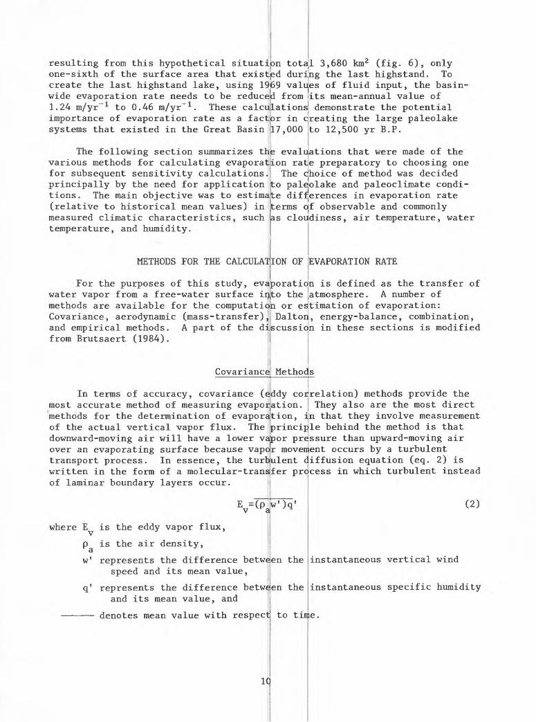
resulting from this hypothetical situation tota.! 3,680 km2 (fig. 6), only one-sixth of the surface area that existed during the last highstand. To create the last highstand lake, using 1969 values of fluid input, the basin- wide evaporation rate needs to be reduced from iits mean-annual value of 1.24 m/yr" 1 to 0.46 m/yr" 1 . These calculations^ demonstrate the potential importance of evaporation rate as a factpr in creating the large paleolake systems that existed in the Great Basin 17,000 to 12,500 yr B.P.

IThe following section summarizes the evaluations that were made of the

various methods for calculating evaporation rate preparatory to choosing one for subsequent sensitivity calculations. 1 The cjhoice of method was decided principally by the need for application to paleiolake and paleoclimate condi­ tions. The main objective was to estimate differences in evaporation rate(relative to historical mean values) in measured climatic characteristics, such temperature, and humidity.

terms qf observable and commonlyas cloudiness, air temperature, water

METHODS FOR THE CALCULATION OF EVAPORATION RATE

For the purposes of this study, evaporation is defined as the transfer of water vapor from a free-water surface ifyto the .atmosphere. A number of methods are available for the computation or estimation of evaporation: Covariance, aerodynamic (mass-transfer), Dalton, energy-balance, combination, and empirical methods. A part of the discussion in these sections is modified from Brutsaert (1984).

Covariance Methods

In terms of accuracy, covariance (eddy correlation) methods provide the most accurate method of measuring evaporation. They also are the most direct methods for the determination of evaporation, in that they involve measurement of the actual vertical vapor flux. The principle behind the method is that downward-moving air will have a lower vajpor pressure than upward-moving air over an evaporating surface because vapor movement occurs by a turbulent transport process. In essence, the turbulent diffusion equation (eq. 2) is written in the form of a molecular-transfer process in which turbulent instead of laminar boundary layers occur. \\

E =(p w f )q f v *a ^ (2)

where E is the eddy vapor flux,

p is the air density,

w 1 represents the difference between the instantaneous vertical windspeed and its mean value,

11 q 1 represents the difference between the instantaneous specific humidity

and its mean value, and

denotes mean value with respect

1C

to time.

120° 119° 118° 117° 116°

42'

41'

40°

39C

38 C

LAKE TAHOE

CARSON RIVER \

100 KILOMETERS

1 50 MILES

AREA COVERED BY SURFACE- WATER BODY

SILL OVER WHICH SPILL OCCURS

Figure 6. Hypothetical surface areas of lakes in the Lahontan basin if the runoff and precipitation that occurred in 1969 became the mean.

11

Turbulence consists of individual eddies; having the same function in turbulent transfer that individual molecules have in molecular transfer. These eddies are responsible for the vertical transfer of heat and water vapor. In prac­ tice, the evaporation flux, E , is determined by measuring the fluctuations, w' and q'.

Aerodynamic (Mass*Transfer) Method

The bulk-aerodynamic equation is eXpresse fl as (Quinn, 1979):

(3)

where E is evaporation rate,

p is air density,3

C is bulk-evaporation coefficient,

q is saturation-specific humidity at water-surface temperature,

q is specific humidity, and

u is wind velocity.

Quinn (1979) showed that the bulk-aerodynamic equation is similar to the classic mass-transfer equation (U.S. Geological Survey, 1954):

E=C (e -e )u mo. a

where C is mass-transfer coefficient,m '

e is saturated vapor pressure atithe water-surface temperature, and

e is vapor pressure of ambient aLr.

(4)

In both equations, evaporation is consi dered proportional to wind speed andvapor-pressure (humidity) difference. The coefficient of proportionality represents a combination of many variables, such as size of the lake, roughness of the water surface, kinematic viscosity of the air, and manner of variation of wind speed with height (Harbeck, 1962).

The Daltoft Concept

Brutsaert (1984) recently discussed Dalton's (1802) contribution to the development of evaporation theory. Dalton recognized the state of evaporation is increased by: (1) Increasing water-surface; temperature; (2) increasing wind speed; and (3) decreasing humidity of ambient air.

Dalton's concept in equation form tis:

E=f(u)(eo-ea )

where f(u) is a function of wind velocity, u.

12

(5)

The application of equation (5) to lake evaporation generally involves a wind-speed function of the form (Stelling, 1882):

f(u)=a(l+bu) (6a)or

f(u)=au (6b)

where a and b are empirical constants.

The aerodynamic, mass-transfer, and Dalton-type equations are similar in that evaporation is expressed explicitly as a function of wind speed and the vertical gradient of vapor pressure (or humidity). Evaporation is implicitly a function of water temperature and vapor pressure, in that e is calculated

using the temperature of the water surface (T ), and q is calculated, in part,

using the temperature of ambient air (T ). The equations also are similar in3.

that the unexplained physics of the evaporation process is lumped in the valueof empirical constants (C_, C , a, b) that multiply the (e -e )u term.iii ro o a

Energy-Balance Method

Evaporation can be considered as the link between the hydrologic balance, and the energy balance for any surface-water system. A change in the heat stored in a reservoir or lake is the result of heat gains from radiation and advective processes, coupled with heat losses occurring as the result of evaporation. In equation form, this balance can be expressed as:

Q =R +Q.-Q -Qu-Q (7) xv n ^v xe xh w

where Q is change in stored-energy content of the water body,

R is net-radiative flux density at water surface,

Q is heat flux advected by surface- and ground-water sources,

Q is latent-heat flux in evaporating water,

Q, is sensible-heat flux, and

Q is the heat flux advected by evaporating water.W

Net radiation, R , can be divided into several components:

R =Q (1-R )+Q (1-R )-Q, (8) n s s a a bs

where Q is solar short-wave radiation incident to water surface, s '

R is reflectivity of water surface to short-wave radiation,S

Q is long-wave radiation incident to water surface, a

R is reflectivity of water surface to long-wave radiation, and3.

Q, is long-wave radiation emitted by water surface.

13

To write the energy balance in relations are used:

Qe=P

rPeECK (

where p is density of water undergoing

L is latent heat of vaporization

C is specific heat of water,

T is surface temperature of wate

T, is an arbitrary base temperatu

p is the Bowen (1926) ratio

such that

terras of evaporation, the following

EL,

o -Tb ), and

e'

evaporation,

of wate;r,

undergoing evaporation,

e, and

E=Q +Q +Q -(Q +Q s xa v xr arp [L(l+0)+C (T -T, re r w o 1

where Q =R Q , short-wave radiation ref r s s'Q =R Q , long-wave radiation refl ar a a' 6

The components of equation 12 can parameterization of each component in t and empirical formulae (for example, U. 1954; U.S. Geological Survey, 1958; Rei others, 1975; and Berger, 1978). By using the formulae, the rate of evaporation can b able climate parameters: (1) Amount of (3) air temperature, (4) water temperature humidity), and (6) solar irradiation inc

Combinati

This description usually is given derived from a combination of energy-ba of the most widely used combination equ (1948):

E=A ~

cn~ A-

where A is slope of the saturation-wate temperature, T ;

Y is psychrometric constant; and Q is available energy-flux densit;

vaporization.

14

ected

cted by

(9)

(10)

(11)

(12)

by water surface; and

water surface.

be obtained by measurement, or by a rms of a combination of theoretical . Geological Survey, 1954; Houghton, an, 1963; Kasten, 1966; Davies and

n Methods

theoretical and empiricalestimated from values of six measur-

sky cover, (2) type of sky cover, (5'l dew-point temperature (or

ident on the upper atmosphere.

o a group of semiempirical methods ance and Dalton-like approaches. One tions is that derived by Penman

vapor-pressure curve at air

divid

(13)

5d by latent heat of

The E. term is of the form:A

EA=f(u)(es -ea ) (14)

where e is the vapor pressure of saturated air at ambient air temperature; sand f(u) (wind function) generally has been formulated in terms of a Stelling- type equation (eq. 6a).

In his derivation, Penman (1948) assummed that the advection (Q ) and

storage (AQ ) terms of the energy-balance equation (eq. 9) were negligible.

He also made the assumption that the saturation vapor-pressure curve varied linearly with temperature between the temperature of the water surface, T , and the temperature of the air at the level of measurement, T ,:

(15)

One advantage of the Penman equation is that it only requires measurement of humidity, wind speed, and temperature at one level. Another advantage is that it can be used with standard climatological data.

Slatyer and Mcllroy (1967) suggested that the first term of equation 13 represented a lower limit to evaporation. They reasoned that, when air has been in contact with a wet surface over a long distance, it will become vapor- saturated, and the value of EA in the second term of equation 13 will tend to be zero, such that:

E_A5n (16)E"An-Priestly and Taylor (1972) used equation 16 as the basis of an empirical

relation for evaporation from a wet surface under assumed conditions of vapor saturation. They determined that for large water surfaces, presumably free from advective processes that would tend to reset the vapor-pressure deficit, equilibrium was best described by:

where values of Q usually range from 1.26 to 1.28. Brutsaert (1984) noted this implies, over large wet surfaces, large-scale advection processes still account for 21 to 22 percent of evaporation.

15

Empirical

A large number of empirical methods tion of evaporation from water surfaces parameters, such as humidity or air temp application, a number of authors (Leopold Orr, 1958; Snyder and Langbein, 1962; Ga Brakenridge, 1978; and Mifflin and Wheat evaporation and precipitation responsibl paleolake systems of probable late-Wisconsin ag method used by these authors to estimate to include the following steps.

have been developed for the estima- ising commonly measured meteorological jratureu In terms of paleoclimate

1951; Antevs, 1952; Broecker andLloway, 1979)

» for tie maintenance of variousThe empirical-estimation

evaporation rate can be generalized

(1) Some indicator of the location(cirque-excavation features, rhollows) was used to estimate depression relative to the timberline)

of past snowline or timberline lict-cryogenic deposits, or nivation he amojnt of snowline (or timberline)

location of modern snowline (or

(2) Location of the modern snowlin seasonal value of temperature the -6 °C annual isotherm).

(3) A constant-value temperature lapse rate level meteorological data and other data, was used to estimate the air- with snowline depression.

(4) The same air-temperature decre drainage basin also was assumed the lake.

(5) The mean-monthly air-temperaturewithin the calendar year either by mean-monthly temperature, with the decrease in January, or by imposing a air temperature.

(6) A correlation between values o temperature (at lake-surface a attempted and applied to the p fig. 7).

Early development and application oestimation of evaporation by certain Snyder and Langbein, 1962) stimulated responsible for paleolake highstands. assumptions on which it was based were rof these seminal papers. Unfortunately,generally have left unexamined theoutlined before. The assumptions are examined

Methods

1970; Reeves, 1973;have attempted to estimate the

was the

correlated with some mean- suinmer 0 °C, the July 0 °C, or

based sometimes on ground- times on free-air radiosonde temperature decrease associated

ase in the high-altitude part of the to have occurred at the altitude of

decrease usually was distributed imposing a graduated decrease of maximum decrease in July and no

uniform decrease in monthly

: mean-annual or mean-monthly air .titudes) and lake-evaporation rate was aleolakfe system (see, for example,

autlors consider;

cogni: authors

assumptions

these empirical procedures for the (especially Leopold, 1951, andtion of the climatic conditions

The shortcomings of the method and the ed and clearly stated in both

of subsequent papers underlying the general method in the following section.

(/D DC LU

LU5

Z

0.4

0.3

DCO Q_

LU

5X

Z O

LU

0.2

0.1

I05 10 15 20 25 30 35

MEAN MONTHLY AIR TEMPERATURE, IN DEGREES CELSIUS

Figure 7.--Relation of evaporation and temperature in the western United States (modified from Galloway, 1970).

Assumption 1: The time of maximum snowline depression is coincident with the time of highest lake stand.

Highstands of large lake systems located in the western United States between 38° and 42° N latitude lag the last continental glacial maximum by periods ranging from 1,000 to 4,000 years (fig. 2). Few data exist on the timing of montane glaciation and deglaciation. Therefore, temperature esti­ mates for times of snowline depression are not necessarily applicable to times of high lake level.

Assumption 2: Free-air and ground-level lapse rates are identical.

Dohrenwend (1984) recently reported that free-air lapse rates are not representative of temperature variation with altitude measured at ground level.

17

Assumption 3: Temperature-Iapse rates ar<3 constant in time and space.

Dohrenwend (1984) suggested the following ture variation with altitude, based on areas in the western United States and (1975): Below 300 m above basin floors mately zero; above 300 m, mean annual 1 altitudes below 2,000 m and -0.76 °K/100 m for Dohrenwend (1984) suggested that the la not a constant, as assumed by previous \

generalized model of tempera- mpirical data from eight mountain m the work of Houghton and othersmean annual lapse rates are approxi-

pse rates are -0.057 °K/100 m foraltitudes above 2,000 m.

])se rate changed with altitude and was workers.

near )ytimes

(leat

However, even this lapse-rate mode level and mountain glaciation. During altitudes would be affected by the above the lake would be affected by the the lake; that is, both the highstand boundary conditions that "buffer" the lapse rate Therefore, any quantitative extrapolation estimates to the surface air mass locat distant basin floors seems tenuous.

lake

Assumption 4: Evaporation is sole. !y a function of air temperature.

theThat this assumption is incorrect

for any mean monthly air temperature, about the mean at any particular time i scatter is not unexpected, as the review day evaporation rates indicates that la of air temperature, but also of water t change in heat stored in the lake.

Comparison of Methods and ChoiceCalculation of Evaporation Rate

In terms of calculating the sensit in one or more commonly measured climat appears the most promising. Each of th energy-balance equation has been shown relation to one or more commonly measur theoretically is sound and, when applied 1 week, has resulted in estimates of eva obtained from water-budget calculations Historically, the energy-balance method evaporation methods have been compared.

The covariance method is of little because evaporation rate is not treated parameters (eq. 2). Mass-transfer and presented in this paper (eq. 3 and 4) that also vary with lake size and way exists of predicting the way the fo past changes in lake size and climate.

18

need uchmass

mass and

of

not apply to times of high laketemperature at high

of glacial ice, and temperature content) of water stored in

the mountain glacier represent in their immediate vicinity,

siiowline air-temperature d immediately above lakes situated on

s shown in figure 7, which shows that range of measured evaporation rates

about 0.12 m. This magnitude of of methods used to calculate present-

ice evaporation is a function not only mperature, humidity, cloudiness, and

of Energy-Balance Method for thefor Usg in Sensitivity Analyses

vity of evaporation rate to variation parameters, the energy-balance method heat terms contained within the

o have a theoretical or empirical d climate parameters. The methodto computational periods greater than

poration rate nearly the same as those(U.S. Geological Survey, 1954).has been the standard to which other

use in studies of past climates in terms of commonly measured climate aerodynamic equations of the form

contain coefficients of proportionality stability. Unfortunately, noatmospheric

rm of the wind function varied with The Dalton and combination equations

are similar in that they contain a wind function (eq. 5, 6a, and 6b) whose form changes with lake size and atmospheric stability. Empirical methods are based on incorrect assumptions, and evaporation rates calculated using them have been determined to be substantially inaccurate. For these reasons, the energy-balance method was chosen for use in the sensitivity analysis.

THEORETICAL AND EMPIRICAL FORMULAE USED IN THE ENERGY-BALANCE METHOD

Solar Radiation

The sun behaves like a black body with a surface temperature of about 6,000 °K. Most of the emitted radiation is within the shortwave band between 0.3 and 3.0 pm. The shortwave irradiation at the upper atmosphere of the Earth, normal to the solar beam, is known as the Solar Constant and has a value of about 1.94 cal cm~ 2 min" 1 . The irradiation is not truly constant; it changes as the Earth's orbit varies in response to lunar and planetary gravitational perturbations (fig. 8).

TIME, IN THOUSANDS OF YEARS BEFORE PRESENT

Figure 8.--Deviations of solar irradiation from their 1950 values at 40° north latitude.

19

Short-wave Radiation

As it passes through the atmosphere tering, absorption, and reflection by pa of solar radiation that reaches the Eartli use of atmospheric-transmission coeffici solar radiation to scattering, absorption

Q =Q*T , Ts da \

solar radiation is modified by scat- cticles and molecules. The proportion

' s surtface may be calculated with the snts that relate the attenuation of

s wa ab

Land surface

is solar irradiation incident o:a the

where Q is solar radiation incident toS

t, is atmospheric-transmission coe da 4.4. scattering,

upper atmosphere,

fficient resulting from dry-air

T is atmospheric-transmissionWS 4.4. scattering,

t is atmospheric-transmission wawater vapor, and

T , is atmospheric-transmission coe (albedo) by clouds.

coefficient resulting from water-vapor

coe Eficient resulting from absorption by

:ficienit resulting from reflection

at anyThe solar irradiation (insolation) a single-valued function of the solar Earth's orbit, its eccentricity, the obliquity helion measured from the moving vernal were obtained from Berger (1978).

Equations for calculation of atmospheric-transmission coefficients are given in Davies and others (1975):

T, =0.972-0.8262M+0.00933M2 da

T =l-0.0225Wp ws

T =1-0.007 wa

dew-point temperature (T, ) through an

W=exp[0.1102+(0.06l3

and the mean optical air mass (M); that by the solar beam. M can be approximated Kasten (1966):

M=l/[sin(90°-Z)+0.150(90

in which the mean zenith angle (Z) can

cosZ=Q*/[(Sd/d)

2C

and reflection processes:

(18)

constant,

equinox.

given latitude on the Earth is the semimajor axis of the and the longitude of the peri- Values of solar irradiation

-0.00095M3+0.0000437M4

and

0.3(WM)

(19)

(20)

(21)

W, the precipitable water vapor aloft, car be related to measured surfaceequation formulated by Reitan (1963):

8(Td -273.15))]; (22)

is, the depth of atmosphere traversed with an equation formulated by

°-Z+3.&85)" 1 - 253 ]

e calculated using

(60t)]

(23)

(24)

where S is solar constant,d/d is ratio of the mean Earth-sun distance to instantaneous distance, and

t is duration of sunshine at any specific latitude.

Sunshine durations are tabulated in List (1951) and also can be calculated using an algorithm derived by Swift (1976).

The atmospheric-transmission coefficient resulting from cloud albedo can be calculated from:

fX) (25)

where A, .. is albedo of high-altitude cirrus clouds,

A , is albedo of medium-altitude clouds, ml '

A, 1 is albedo of low-level heap clouds,

f, , is fraction of sky covered by high-altitude clouds,

f , , is fraction of sky covered by low-altitude clouds,

f , is fraction of sky covered by medium-altitude clouds, and

X is total fraction of sky covered by clouds.

Houghton (1954) recommends cloud-albedo values of A, =0.21, A =0.48, and Al;L=0.70.

A part of the solar radiation reaching a water surface also is reflected by that surface:

Ws (26)

where Q is the part of incoming solar radiation that is reflected from watersurface, and

R is solar-radiation reflectivity of the water surface.

Houghton (1954) recommends the use of a value of 0.07 for R .S

Long-Wave Radiation

Long-wave radiation is absorbed and emitted mainly by water vapor, carbon dioxide, and ozone, to a lesser extent. Long-wave radiation incident to a water surface can be approximated by empirical formulae relating radiation to cloud height, cloud amount, and ambient vapor pressure (U.S. Geological Survey, 1954):

Q =Q -+Q n +Q , (27) xa a, hi a, ml xa,ll

Q , =ful oT 4 (au ,+bu ,e ), (28) xa,hl hi a hi hi a '

(29)

(30)

21

where Q , .. is long-wave radiation ' clouds,

0 i is long-wave radiation a,ml _ .clouds,

Q -,, is long-wave radiation ' clouds, and

a is Stefan's constant (a = 11

Additional parameterizations used in equ

ah] =0.74+fhl (0.025x

a =0.74+f ..(0.025X ml ml A

falling on water surface from high-level

falling on water surface from medium-level

falling on water surface from low-level

1(0.025X-

b, =0.00490-f, n (0.000 hi hi

b =0.00490-f ,(0.000 ml ml

b11=0.00490-f11 (0.000

where « is altitude .of high-level

, ,

., ml

clouds (6 kin),

is altitude of low-level clouds (1 km), and

is altitude of medium-level clouds (4

Part of the long-wave radiation reaching

Q =R Q ar a a

where R is long-wave reflectivity of wa3.

recommends a value of 0.03 for '.

Q is the part of incoming long-wa

water surface back to atmosphere

Part of the long-wave radiation to the atmosphere:

Q, =oT 4 xbs o

where e, the emissivity of water, equals 1954).

22

71 x

tions

ll)~ 8 cal cm 2 d' 1 °K~ 1 day)

28-30 are:

"hi),

-0.1916«

-0.19l6oc

ml),

ID,

, -0.1969« _. 4xe hi),

, -O.L9690C _, , 4xe ml), and

(31)

(32)

(33)

(34)

(35)

(36)

km).

the water surface is reflected:

;:er surface; Houghton (1954)

, and

(37)

/e radiation that is reflected from

absorbed the body of water is emitted

(38)

0.970±0.005 (U.S. Geological Survey,

During the process of evaporation, heat is transferred to the atmosphere as latent heat (Q ), sensible heat (Qh )> and advected heat (Q ). These heat fluxes can be calculated from:

Q =p EL, and e re '

Q =p C E(T -T, ). xw re w o b

Because the atmospheric-transport mechanisms of sensible heat and water vapor are similar, the sensible-heat flux generally is treated with the rate of evaporation. The ratio of these fluxes is called the Bowen ratio, (3:

which, combined with equation 9, yields:

Bowen (1926) determined that if water vapor and sensible-heat transport both were expressed in the form of a diffusion equation, the Bowen ratio, (3, would be written in terms of temperature and vapor pressure gradients; that is:

T -T

o a

where y, the psychrometric constant, is given by

and where P is the ambient air pressure, in millibars, and c is the specific heat of air at constant pressure.

Heat reaching the water body by advection (streamflow and overland runoff, ground-water discharge, and precipitation directly onto the water body) can be calculated from a knowledge of the volumes of advected fluids, their temperatures, and their heat capacities:

n0 = I p V.(T.-T,)C (42) ^ r

where p is density of advected water,

V. is volume of the ith source of advected water integrated over any convenient time, and

T. is mean temperature of the ith source of advected water averaged overthe time used to calculate V. .i

23

A change in the heat stored in the water the sum of the individual heat-transfer proces calculated from a knowledge of the mean temperature of the body of water. This calculation usually dividing the body of water into a number of lay heat content of each layer is calculated, and are summed:

kQ = I p.C (T. v _._ 1 Kj v -

where p. is density of the jth layer of_J

T. is mean temperature of the jthJ

Ax. is thickness of each layer of

A. is area of the jth layer of wa

body can occur as the result of es. The stored heat can be

, heat capacity, and volume is made by vertically sub-

ers of equal thickness. The the heat contents of all layers

In certain situations, the time ove calculated can be chosen so that AQ =0.

over a time starting and ending with th For certain situations, the advection h

example, the temperature of much of the 0 °C (the base temperature in our compu transported by such streams tends to be terms in the energy-balance equation, can be carried out over a time for whici equivalent to the increase of stored

T. J

of

th

f

wa

ov0.

thL h

hetpube

tiche

-VAx.

water,

layer

tfater,

ter .

er whicFor e

e lakeeat ter

runofftationssmallfinallyi the aat, sue

A. (43)J

of water,

and

i the energy balance isxample, the balance can be made

in the same isothermal state.m, Q , also can be ignored. For

from the Sierra Nevada is near); therefore, the heatin comparison to the other heat, the heat-balance calculationddition of advected heat ish that:

AQ -Q =0.

Having established theoretical anc the energy balance (eq. 9 and 10) in terms of(eqs. 11 through 43), the sensitivity of evaporation rate to changes in each of six climate parameters--(1) amount and (2) temperature, (4) water temperature, ( and (6) solar irradiation incident on the determined.

SENSITIVITY ANALYSIS

lake-

For the sensitivity analysis, a to be established. The lake chosen as (fig. 1 and table 3). The reference land-based mean monthly meteorological weather station (U.S. Weather Bureau, 1 Atmospheric Administration, 1966-75) measurements made at Pyramid Lake reference sky was assumed to be composed

arid during

(44)

empirical relations for components ofmeasurable climate parameters ration rate to changes in e type of sky cover, (3) air

dew-point temperature (or humidity), upper atmosphere now can be

950-65

reference; lake-climate system first needs a reference site was Pyramid Lake, Nev.

-climate system was a composite of data recorded at the Reno, Nev.,

National Oceanic and laketbased water-surface temperature 1976 and 1977 (Benson, 1984). The of 80-percent high-level clouds,

10-percent medium-level clouds, and 10-percent low-level clouds. A computer program (EVAP, table 4) was used to calculate evaporation rate in terms of the empirical and theoretical relations previously established between the climatic parameters of the reference data set and the heat terms contained in equation 12. The calculated evaporation rate of 1.10 m yr" 1 (table 5) was in reasonable agreement with mean annual evaporation rate of 1.2±0.1 m, deter­ mined by Harding (1965) for 1932-52, using a water-budget method. However, the agreement between the results of the energy-balance and water-budget methods resulted from use of meteorological data recorded at a land-based site located 60 km south of the center of Pyramid Lake. The temperature and relative humidity of air at some standard distance over the land-based site will not be the same over the lake surface. Therefore the agreement between calculated and measured rates of evaporation may be fortuitous.

Table 3.--Reference-climate data set for Pyramid Lake, Nevada

[°K, degrees Kelvin; mb, millibars; cal cm~ 2 day" 1 , calories per centimetersquared per day]

Month

January- ---February---lid I. V,I1

April------May--------

June-------July August-----September--October----

November---December---

Air temper­ ature (°K)

273.0276.4O7Q OZ /O . ZOO 1 OZo 1 . ZOQc oZoD . o

290.0294 2^* j ~ 4+

293.0288.6283.6

277.6273.6

Water temper­ ature (°K)

279.7279.7279.7OQO oZoZ . ZOQC OZoj . Z

289.7O f\ / O294.2294.2293.2290.7

287.2283.2

Sky cover (frac­ tion)

0.65.61CLC

. JO

.55

.48

35* <*s *J

.22

.21

.23

.39

.57

.63

Pres­ sure (mb)

866865Q£QCOOQ£QbooQ£Qobo

Q£ QoboO/T cobj864864865

866866

Opti­ cal air

mass

2.992.572.111.901 Cl1 . o 1

1.701 7Q1 . /o

1.842.012.36

2.833.16

Solar irradiation

(cal cm" 2 day" 1 )

374513690oc ooDZn £ i9bl

996954842680507

372322

Dew- point temper­ ature (°K)

267.4269.6269.1270.6O T / O274.2

277.3279.4279.0276.7273.9

270.7268.4

25

Table 4. EVAP computer program listing

[Abbreviations in table are included in symbols;definitions list at the leginnirig

REAL REAL REAL REAL REAL REAL REAL REAL REAL REAL

SXY(12)/HUMID(12 TAUSCATd 2)/TAUW TAUAL3M 2)/MASSA SVP2M(12)/QA(12) 30WRAT(12)/QBS(1 AH(12)/AM(12)/AL ALBHI/ALBMED/AL3 3AS£T/FRLO(10)/F QV(12)/QNU(12)/Q SUMARY(20/10)/HI

) /kL ETd IRd /QR( 2),L (12) LO/A RHI ( AHd (20/

OFTd 2)/?d 2) / Q S12)/QAHEAT(/3H(1LTHI/a10)/Fq2)/3AN1 0 ) / M 0

CHARACTER * 30 TITLE INTEGER I/LHEAD/J

OPEN (5/FILE =OPEN (o/FILE =OPEN (7/FILE =

'WORK. INI') 'WORK.OUT') 'SUMMARY')

READ(5/102)(FRhl(I),1=1/10)READ(5/102)(FRMED(I)/I=1/10) READ(5/102)(FRLO(I)/I=1/10)

00 1500 J=1/20

READ (5/100) TITLE IF (TITLE.EQ.'QUIT'.OR.TITLEREAD (5/101) (SKY (I)/I = 1/12)READ (5/1G1) (DE'WPT(I) ,1 = 1/12)READ (5/101)(AIRT(I)/I=1/12)READ (5/101)(WATERT(I)/I=1/12)READ (5/*)(QSTAR(I)/I=1/12)READ (5/101)(MASSAIR(I)/I=1/12)READ (5/101)(P(I)/I=1/12)READ (5/101)(QV(I)/I=1/12)READ (5/101)(QNU(I)/I=1/12)

CONSTANTS

ALBHI=.21AL3MED=.48ALBLO=.7GALTHI=6.0ALTMED=4.0ALTLO = 1 .000=6984.505294D1=-133.903931002=2.133357675D3=-1.238530973E-2D4=4.393587233E-5D5 = -8.0239233S2E-<506=6.136820929E-11

variables, dimensions, and of manuscript]

)/AIt?T(12)/WATERT(12)/TAUORY(12)2)/NUM(12)/OENOMd2)/OEWPT(12)12)/Q:5TAR(12)/SVPDEW(12)R(12),'SVPOV(12)2)/MEVAP(12)/ANEVAP)/3M(12)/BL(12)/APWATR(12)LTMEO.-ALTLO/00/D1/D2/D3/04/D5/06M10 (1 0)(12)/OAL(12)0(20/'IO)/LOW(20/10)

it') GO TO 8

2:6

Table 4. EVAP computer program listing Continued

BASET=273.15

WRITE(6,899)N = 000 1100 K=1,10

WRITE (6/98) TITLE

HI(JrK)=FRHI(lO*100.MED(J/K)=FRMED(K)*100.LOW(J,K)=FRLO(K)*100.

WRITEC6/702) HKJ/K)WRITE(6/703) MEQU/K)WRITE(6/704) LOWCJ/K)

WRITE (6/490) ANEVAP=0

00 1000 1=1/12

WLOFT(I)=EXP((.1 10? + .06133*(OEWPT(I)-273.15)))TAU5CAT(I)=1-(0.0225*WLOFT(I)*MASSAIR(D)TAUORY(I)=0.972-(C.03262*MASSAIR(I))*Q.00933*

C (MASSAIR(I)**2)-0.00095*(MASSAIR(I)**3)*C 0.0300437*(MASSAIR(I)**4)

TAUWET(I)=1-(0.077*((WLOFT(I)*MASSAIR(I))**.3)> TAUALd(I)=1-((ALSHI*FRHI(K)*SKY(I))-»-(AL3MEO*FRMED(K)*

C SKY(I))*(ALBLO*FRLO(K)*SKY(I)))QS(I)=QSTAR(I)*TAUDRY(I)*TAUSCAT(I)*TAUWET(I)*TAUALB(I)QR(I)=. 07*35(1)AM(I)=.74*PRMED(K)*(.'025*SKY(I)*EXP(-0.1916*ALTMEO»5M(I)=0.0049-(0.0054*SKY(I)*EXP(-Q.1969*ALTMED))*FRMED(K)AH(I)=.74*FRHI(K)*(.025*SKY(I)*EXP(-0.1916*ALTHI)>AL(I)=.74+FRLO(K)*(.025*SKY(I)*EX3(-3.1916*AITIO))BH(I)=0.0049-(0.0054*SKY(I)*EXP(-0.1969*ALTHI))*FRHI(K)3L(I)=0.0049-(0.005^*SKY(I)*EXP(-0.1969*ALTLO))*FRLO(K)

C (D4+AIRT(I)*(05+C6*AIRT(I))))))SVPOEW(I) = 00 *OEWPT(I)*(01*OEWPT(I)*(D2-«-O

C OEWPT(I)*(04*DEWPT(I)*(05*D6*OEWPT(I)))))) HUMID(I)=SVPDEW(I) / SVP2M(I)

QAH(I)=FRHI(K) * (1.171E-07 * AIRT(I)**4)* C (AHd)* 3H(D* SVPDEW(D)

QAM(I)=FRMEO(K) * (1.171E-Q7 * AIRT(I)**4)* C (AM(I)* BM(I)* SVPOEW(D)

QAL(I)=FRLO(K) * (1.171E-07 * AIRT(I)**4)*

C (ALCD* 3L (I)* SVPOEW(I))QA(I)=QAH(I)+QAM(I)+QAL(I)QAR(I)=0.0301*QA(I)QBS(I)=1.171E-07*(WATERT(I)**4)*0.97LHEAT(I)=(-0.57*WATERT(I))*753.1SVPOM(I) =DO+WATERT(I) *(D1*WATERT(I)*(D2*WATERT(I)*

C (D3*WATERT(I)*(D4-»-WATERT(I)*(05*06*WATERT(I))))))BOWRAT(I)=0.61*(WATERT(I)-AIRT(I))/((SVPOM(I)-SVPOEW(I))*

27

1000

1111

1100

1500Cc

3

Table 4. EVAP comput

C C1000/PCINUM(I)=QSCI)+QACI)OENOM(I)=(LHEAT(I)MEVAP(I)=(NUM(I) /DANEVAP=MEVAPCI)+ANARWATR(I)= WATERTC

CONTINUEANEVAP=ANEVAP/100SUMARYCJ,K)=ANEVAPWRITEC6/90Q)WRITEC6/304) CAIRTCI)/I=WRITEC6/305) CWATERT CI )/WRITEC6/301 ) CSKYCI),I=1WRITEC6/311 ) (PCI), 1=1 /1WRITEC6/310) CMASSAIRCI)WRITEC6/309) CQSTAR(I) ,1WRITEC6/495)CDEWPT(I)/IWRITECo/^90)WRITEC6/423) CARWATRCI)/WRITE C6/ 30 2) CHUMIOCI) /IWRITEC6/303) CWLOFT(I) /IWRITEC6/45Q)CLHEAT(I)/IWRITEC6/306) CTAUORY(I),WRITEC6/307) CTAUSCATCI)WRITEC6/303)CTAUWET(I),WRITEC6/411 ) (TAUALB (I )/WRITEC6/455) CSVPDMCI) /IWRITEC6/456) CSVP2MCD/IWRITE C6/457)CSVPO£W CD/WRITEC6/412) CQSCI)/I=1/WRITEC6/420) CQRCI)/I=1,WRITEC6/417) CQBSCI) /I=1WRITEC6/458) (QAHCI)/I=1WRIT EC 6/459) CQAMCI) /I=1WRITEC6/460) (QAL(I) /I=1WRITc(6/41 5) (QACI) /I=1,WRITEC6/41&) CCARCI)/I=1WRITE(6/461 ) (QV(I),I=1,WRITE(6/462) (QNU(I)/I=1WRITE (6/41 8) (BOW RAT (I),WRITEC6/421 ) CNUMCI) /I=1WRITEC6/422) CDENOMCD/IWRITEC6/490)WRITEC6/425) CMEVAPCI) /IWRITEC6/485) ANEVAPWRITEC6/399)

CONTINUE

CONTINUETHIS NEXT SECTION IS TO SUTHE DATA FILE IS CLOSED AN

CONTINUE

REWINOC5)

*r program listing Continued

))+QV(I)-(QR(I)+QAR<I)+QSS(I)+QNU(I)*C1+BCWRATCI)))+CWATERT(I)-3ASET)ENOM(I))*39.42EVAPI) - AIRTCI)

1/12)1=1/1^)/12)2)/I=1/12)=1/12)=1/12)

1=1/12)= 1/12)= 1/12)!=1/12)1=1/12)/I=1/12)1=1/12)1=1/12)=1 /12)=1/12)1=1/12)12)12)/12)/12)/12)/12)12)/12)12)/12)1=1/12)'12)=1/12)

=1/12)

IMARUE THt EVAPORATION RESULTSD REOPENED FOR THE TITLE

28

Table 4. EVAP computer program listing Continued

94

96

DO 11 J=1,20IF (J ,LT. 2)GO TO 94READ (5,97,END = 999,ERR = <*99) TITLEGO TO 96READ (5,99,END=999,ERR=999) TITLE

201198979910010110210330130230330430530630730830931031141 1412415416417418420421422423425450455456457458459460461462465466

485

WRITEC7, 00 23 K = 1,

WRITEC7, WRITEC7, WRITEC7,

CONTINUE CONTINUEFORMATC13X,FORMATU80,FORMAT(3C/)FORMAT(ASO)FORMATdFORMATdFORMATC5FORMATdFORMATdFORMATdFORMATdFORMATdFORMATdFORMATdFORMATdFORMATdFORMATdFORMATdFORMATdFORMATdFORMATdFORMATdFORMATdFORMATdFORMATC1XFORMATdFORMATdFORMATdFORMATdFORMATdFORMATdFORMATdFORMATdFORMATdFORMATdFORMATdFORMATdFORMATdFORMATdFORMATdH

F4FORMATdH

899) 10465)TITLE466)HI(J,K),MEO(J 485)SUMARY(J,K)

A80)

A80

K),LOW( J,K)

12F6.2)10F4.3)5F6.2,F7.2,1 X,'SKY1X, 'HUMID1X,'WLOFT1X,'AIRT1X,'WATERT1X,'TAU OA1 X , ' T A U W S1 X , ' T A U W A1X,'QSTAR1X,'MASSAIR1X,'P1X,'TAU AB1X,'QS1X,'QA1 X, 'QAR1X,'Q5S1X,'30WRAT1X,' QR1X,'NUM1 X,' JENOM1 X,'WATERT-1 X,'MEVAP1 X,'LHEAT1 X,'SVPOM1 X , ' S V P 2 M1X,'SVPDEW1 X,'QAH1 X,' QAM1 X,'QAL1 X , ' Q V1 X,'QNU1HO/3X/A80)1H ,15X,F4.F4,1,'% MED1H ,20X,'M£

6F6.2)',12F6.2)',12F6.2)',12F6.2)',12F6.1)*,12F6.1 )',12<=6.2)',12 C 6.2)'/12F6.2)',12F6.0) /12F6.2)'/12F6.0)',12F6.2)'/12F6.O'/12F6.0)'/12F6.0)'/12F6.0)',12F6.3)',12«=6.0)',12F6.1:',12F/D.O)

AIRT',12F6.1)',12F6.2)',12F6.1 )',12F6.2)',12F6.2)

',12F6',12F6.0)',12=0.0) /12F6.0)',12F6.2)'/12F6.2)

1,'% HI CLOUDCLOUDS', /1H

AN ANNUAL EVA

2)

S',5X,,25X,F4.1,'% LOW CLOUDS')

EVAPORATION =',F8.3,' M/Y')

29

490495702703704899900

999

Table 4. EVAP computer

FORMATdHO)FORMATdX^'OEWPT ',12F6FORMATdH *30X,F4.1/' PERCENFORMATdH ,30X,F4.1/' PERCENFORMATC1H ,30X/F4.1/' PERCENFORMAT (1H1)FORMAK6X/-' JAN FE3

SEP OCT NOV DEC')

^ * * M. ^ v / f f ^

prograi

.1)T Ht JT MEDlT LOW

MAR

i listing Continued

;LOUDS'):UM CLOUDS')CLOUDS')

APR MAY JUN

ENDFILE ENDFILE

CLOSE (6) CLOSE (5) CLOSE (7)

(7)

9999 STOPEND

JUL AUG

30

Tabl

e 5. Co

mput

ed evaporation

rate

s, in

met

ers

per

year

for

fractions

of clou

d ty

pe,

amount of

sky

cove

r,

and

vari

ous

combinations of

ai

r te

mper

atur

e, wa

ter

temp

erat

ure,

an

d relative hum

idit

y

[Val

ues

of solar

irra

diat

ion

are

for

12,000 years

befo

re pr

esen

t, unless ot

herw

ise

noted,

f,,

, fr

acti

on of

hi

gh-l

evel

cl

ouds

f , fraction of

me

dium

-lev

el cl

ouds

; f

, fraction of lo

w-le

vel

clou

ds;

°K,

degr

ee Ke

lvin

]

Fractions

ofcloud

type

fhl>

0.80 .70

.70

.60

.60

.50

.50

.50

.40

.33

0.80 .70

.70

.60

.60

.50

.50

.50

.40

.33

0.80 .70

.70

.60

.60

.50

.50

.50

.40

.33

0.80 .70

.70

.60

.60

.50

.50

.50

.40

.33

f ,,

f ml'

0.10

0.

.20

..10

..30

..20

.

.40

..30

..20

..30

..33

.

0.10 0.

.20

..10

..30

..20

.

.40

. .30

..20

..3

0 .

.33

.

0.10 0.

.20

..10

..30

..20

.

.40

..30

..20

..30

..3

3 .

0.10 0.

.20

..10

..3

0 .

.20

.

.40

. .30

..20

..30

..33

.11 10 10 20 10 20 10 20 30 30 33 10 10 20 10 20 10

20 30 30 33 10 10 20 10 20 10 20 30 30 33 10 10 20 10 20 10

20 30 30 33

Incr

ease

in

amount

0 pe

rcen

t

1 1 1 1 1 1 1 1 1 0 0 0

.166

.139

.117

.112

.090

.085

.063

.041

.014

.986

.753

.732

.715

.711

.694

.690

.673

.656

.635

.576

.639

.617

.599

.595

.577

.573

.555

.538

.516

.494

.569

.549

.533

.529

.513

.509

.493

.477

.458

.438

10 pe

rcen

tin

Ja

nuar

y

1.13

51.105

1.081

1.076

1.05

1

1.04

61.

021

.997

.967

.936

0.72

9.7

06.6

88.6

83.6

65

.660

.641

.622

.599

.576

0.614

.590

.570

.565

.546

.541

.521

.502

.478

.453

0.547

.525

.507

.503

.486

.482

.4

64.4

46.424

.403

of sk

y co

ver

rela

tive

to re

fere

nce

10 pe

rcen

tin

August

1.124

1.094

1.069

1.063

1.038

1.032

1.007

.982

.951

.920

0.719

.695

.675

.671

.652

.647

.6

28.6

08.584

.559

0.607

.582

.561

.557

.536

.532

.512

.491

.467

.442

0.537

.514

.495

.491

.473

.468

.450

.431

.409

.386

20 pe

rcen

tin Ja

nuar

y

1.104

1.07

11.044

1.039

1.01

2

1.00

6.9

79.9

52.9

19.886

0.70

6.6

81.6

60.6

55.6

35

.630

.609

.588

.563

.537

0.589

.562

.541

.535

.514

.509

.487

.466

.439

.413

0.52

5.5

01.482

.477

.458

.453

.434

.415

.391

.367

10 pe

rcen

teach month

1.094

1.06

11.

033

1.02

71.000

.994

.966

.939

.905

.871

0.696

.670

.649

.644

.623

.618

.5

96.5

75.5

49.5

22

0.58

2.5

55.5

33.5

28.506

.500

.478

.456

.429

.402

0.51

6.491

.471

.466

.446

.441

.4

21.4

01.376

.352

data se

t (table 3)

20 pe

rcen

tin August

1.083

1.04

91.

021

1.015

.987

.980

.952

.924

.889

.854

0.685

.659

.636

.632

.609

.604

.582

.560

.533

.505

0.57

5.5

47.524

.519

.496

.491

.468

.446

.418

.390

0.505

.479

.459

.454

.433

.428

.4

07.386

.361

.335

20 pe

rcen

tea

ch month

1.022

.983

.949

.943

.910

.902

.869

.836

.796

.756

0.63

9.6

08.582

.577

.551

.545

.520

.493

.462

.430

0.526

.493

.467

.460

.434

.428

.401

.375

.342

.310

0.463

.433

.409

.403

.379

.373

.3

49.3

25.2

95.2

66

Variations in

ai

r te

mper

­ature, wa

ter

temperature,

and

rela

tive

humidity

Values for

air

temp

era­

ture

, water

temperature,

and

rela

tive

humidity

taken

from

reference

data set

(table 3).

Valu

es for

air

temp

era­

ture re

duce

d 5°

K and

values fo

r relative

humidity increased

20 pe

rcen

t each month

relative to

re

fere

nce

data

se

t (t

able

3)

.

Valu

es fo

r ai

r tempera­

ture

re

duce

d 15 °K

in

July an

d no

re

duct

ion

in Ja

nuar

y relative to

refe

renc

e da

ta se

t(t

able

3)

.

Valu

es fo

r ai

r tempera­

ture

re

duce

d 10

°K

an

dva

lues

fo

r relative

humidity in

crea

sed

10 percent

each m

onth

relative to

re

fere

nce

data

se

t (t

able

3).

Parameter

Eight parameters: (1) Air temperature (T

(3) amount of sky cover (x); (4) solar irradia (QvV ); (5) fraction of high-level clouds

clouds (f _); (7) fraction of low-level clouds mltemperature (T, ) were varied in the sensitivi

dewpoint temperatures were adjusted toin relative humidity (RH). Dewpoint temperatureair and water temperature by adjusting the ambient

:orrespond to simple percentage changes was varied independently of

vapor pressure.

Four types of parameter distributions wer of distribution, the same change or set of monthly reference state. Examples are a decrease temperature, and a 20-percent increase :Ln the

The second type of distribution wa (or increase) in a parameter each month increase) in July or August and no redu decrease of 10 °K in the July air tempe January air temperature, and a 20-percent incr no increase in January sky cover. Mean tribution were calculated using an equation of

characterized by a scaled reduction with the maximum reduction (or

:tion ipi January. Examples are a rature, with no reduction in the

ease in August sky cover, with monthly values for this type of dis-

x -(xo-x.) +x.O

where X. is historical mean monthly

X. is maximum mean monthly value

X is minimum mean monthly value

increaseAX. is maximum reduction (or iJ of X, and

X.+AX. is scaled value of parameter X

The third type of distribution was sky cover each month, with the maximum August. Mean monthly values for this equation of the form:

AX

X -X. v o i' iL o j

where all symbols have been previously increase applied to the January value.

32

Variation

); (2) water temperature (T );

tion at the upper atmosphere (6) fraction of medium-level

(f,,); and (8) dewpoint

ty study. Variations in

e employed. In the first type conditions was imposed on the

of 5 °K in mean monthly air absolute mean monthly sky cover,

the form:

=X.+AX. i i (45)

value for parameter X,

or parameter X,

or parameter X,

) made to July (or August) value

for the ith month.

characterized by a scaled increase in increase in January and no change in

distribution were calculated using an

=X.+AX

define^, except AX , the maximum

(46)

The fourth type of distribution was used for the solar-irradiation param­ eter (Q*). Three distributions of this parameter were assigned, corresponding to three specific times: 1950, 12,000 yr B.P., and 18,000 yr B.P. (table 6). The data for 1950 represent the present reference state; the data for 12,000 yr B.P. represent the time at or shortly after maximum lake levels recorded in the Lahontan and Mono basins; and the data for 18,000 yr B.P. represent the time of maximum worldwide glacial accumulation (fig. 2). In terms of seasonal deviation of solar irradiation, the situation 18,000 yr B.P. was very similar to the situation in 1950; however, winter solar irradiation was at a minimum, and summer solar irradiation was at a maximum 12,000 yr B.P. (fig. 8).

Table 6.--Solar irradiation for the 21st of each month at 40° north latitude for 1950, 12,000 years before

present, and 18,000 years before present

[yr B.P., years before present]

_______Calories per centimeter squared per day_________Date 1950 12,000 yr B.P. 18,000 yr B.P

January 21----February 21---Marrh 91------I let i. l~J.l ^. J.

April 21 May 21

June 21 July 21 August 21-----September 21--October 21

November 21---December 21---

374513690Or oODZ

961

996954-/ *J T

842680507

372322

343489/T Onoo9QR7OO /

1,030

1,0801,024

879682484

341289

373521711QQ/iOO't

994

1,019958829660488

359315

A listing of the various parameter distributions, as well as the change allotted to a given parameter used in the sensitivity analysis, is shown in table 7. Note that values for dew-point temperature have been replaced with equivalent values of relative humidity to aid the reader in understanding the magnitude of the change in terms of a familiar parameter.

Mean optical air mass (M), and air pressure (P), are relatively invariant with time; therefore they were held constant in the sensitivity analysis. For the purpose of the sensitivity analysis, the advected heat energy was assumed equal and opposite in size to the mean annual change in stored heat energy (eq. 43).

33

Table 7.--Values of parameters used

to[Values refer to differences relative following value indicates time at which scaled-parameter distribution; °K, deg

level clouds; f -. , fraction of medium

hi'

-level clouds; f

rapin evaporation-sensitivity analysis

reference data set (table 3); monthdifference was maximized for a

rees Kelvin; f^-, , fraction of high-

fraction of low-level clouds]

Air Water Relative temperature temperature humidity

(°K) (°K) (percent)

000-5 July -5 July -10

-10 July -10 July -20 -15 July -5 +10

-5 -10 +20 -10

Parameter C

In the sensitivity analysis, the r using three different values of Q* combf,.. : f , : f , n (tables 6 and 7). Havi hi ml 11evaporation rate, all subsequent comput 12,000-yr B.P. value of Q*, combined wi of T T RH, X , and f : f : f

a U 11 J_ lllx J-J-

calculations were made, using the EVAP program represents a major refinement t developed by Benson (1981). Improvemen

1. Incorporation of more accurateterms of T and T, (Lowe, 1977); a dp

2. Explicit treatment of the depe

3. Inclusion of the dependence ofan ;

4. Values of Q* based on a solar

5. Use of the EVAP computer progr energy-flux balance, except Q and AQ .

Sky- amo (per

+10 A +20 A +10 J +20 J

+1+1+2

ombinat

eferenc ined wi ng demo

er calc th vari A tota

compute o an ea ts incl

series

ndence

Qa on

constar

am to c

4

' 11'

cover Cloud Typeunt f f f cent) hi ml 11

0 0.80 0.10 0.10ugust .70 .20 .10 ugust .70 .10 .20 anuary .60 .30 .10 anuary .60 .20 .20 0 .50 .40 .105 .50 .30 .200 .50 .20 .30

.40 .30 .30

.33 .33 .33

ions

e data set (table 3) was run, th the nine variations in nstrated the effect of Q* on

ulations were done, using the ous combinations of the values 1 of about 6,000 evaporation

r program. The EVAP computer rlier energy-flux balance model ude:

approximations for e and e in s a

of RH on both T and T , ; a dp

fui , f , , f T ., , a, T , a T , and hi' ml' 11 hi' ml'

it of 1.94 \ min' 1 ; and

alculate all components of the

Results of Sensitivity Analysis

In former studies (for example, Galloway, 1970), great emphasis has been placed on decrease of evaporation rate due to air-temperature reduction. However, the sensitivity analysis showed that evaporation rate does not change when both T and T are reduced by equal amounts. For example, reduction of

3. O

both July T and July T by 10 °K resulted in a calculated evaporation rate of a o1.18 m yr" 1 , which is nearly identical to the rate calculated using reference- state data that is, 1.17 m yr" 1 . Therefore, the difference between T and

aT --that is, T -T --is the fundamental thermal parameter affecting evapora- o a otion. A change in air temperature alone does not necessarily indicate a change in evaporation rate.

Certain computed evaporation data sets are given in table 5. The data are ordered so the maximum computed rate of evaporation is located at the upper left of the table, and the minimum computed rate of evaporation is located at the lower right of the table. The range of computed rates is significant, ranging from 0.266 to 1.166 m yr" 1 .

The response of the computed evaporation rate to change in each of the climate parameters is summarized in figure 9. Several conclusions can be drawn from these data:

1. Evaporation rate is most dependent on the thermal parameter, T -T .a o

For example, monthly decreases of 5 and 10 °K in T -T result in evaporation-

rate reductions of 0.35 and 0.58 m yr" 1 .

2. Use of solar-irradiation values for 12,000 and 18,000 yr B.P. result in small increases in the computed rate of evaporation.

3. Relatively large absolute changes in relative humidity (RH) result in rather small changes in the computed rate of evaporation. For example, an extrapolated monthly increase of relative humidity by 40 percent increases the relative humidity of the dryest month (July) to 64 percent, while 4 of the more humid months acquire humidities in excess of 95 percent; however, the calculated mean annual evaporation rate decreases by only 0.06 m.

4. Change in the fractional distribution and absolute amount of sky cover can result in a significant reduction in the computed evaporation rate.

POSSIBLE CAUSES OF EVAPORATION-RATE REDUCTION IN THE LAHONTAN BASIN14,000 TO 12,500 YEARS AGO

It has been stated previously that, given a mean-annual fluid input to the Lahontan Basin equivalent to the fluid input occurring in 1969, the creation and maintenance of the last highstand lake necessitated a reduction in evaporation rate to 0.46 m yr" 1 . The following discussion will attempt to associate the reduction of evaporation rate to changes in certain climate parameters.

35

1.2

ii? CCK < < £cc >-

§1

P GL

Aj

~Solar Irradiation Change

-.1950

6 12 18

TIME IN THOUSANDS OF YEARS BEFORE PRESENT CHANGE

HUMID!IN RELA1

Y, IN PERCENT

t .20 Q

.05

.10

.15

0.8/0.1/0.1 fhl/fml/fll

I 0.7/0,2/0.1

0.7/0.1/0.2

0.6/0.3/0.2

0.5/0.3/0.2

0.5/0.2/0.3

0.4/0.3/0.2'

0.3/0.3/0.3

40

WE

CHANGE IN FRACTION OF CLOUD COVER TYPE INCREASE IN AMOUNT OF

CLOUD COVER, IN

Figure 9. Evaporation as a fun B, relative humidity (RH); C, level clouds (f^-,), fraction fraction of low-level clouds and E, AT -T , increase in th(T ) and water temperature (T a i

ofztion cloud-

of medium

PERCENT

EXPLANATION

fhl/fml/fll 0.8/0.1/0.1 ON ALL FIGURES EXCEPT C

C INDICATES SOLARIRRADIATION IN 1950

INDICATES SOLARIRRADIATION 12,000 YEARS BEFORE PRESENT

« INDICATES SOLAR IRRADIATION 18,000 YEARS BEFORE PRESENT

0 5 10 15 20

INCREASE IN AIR TEMPERATUREWATER TEMPERATURE

DIFFERENCE, IN DEGREES

A, solar irradiation (Q*); cover type fraction of high-rlevel clouds (f ,), and

D, amount of sky cover (x); difference between air temperature

).

Air Temperature

Results of paleobotanic and geomorphic studies, previously cited, indicate a decrease of mean annual air temperature by 7 °K. Results of the sensitivity analysis (summarized in fig. 9) indicate that reducing the mean monthly air temperature by 7 °K results in a decrease of evaporation rate to0.72 m yr" 1 , with f, , : f , : f,, set to 0.8 : 0.1 : 0.1, and lake-surface J ' hi ml 11 'temperatures set to present-day values. If the 7 °K reduction in mean annual air temperature is distributed in a scaled manner, with a maximum reduction of 15 °K occurring in July, and no reduction occurring in January, and under the same conditions of water temperature and fractional sky cover as stated previously, the evaporation rate is reduced to about 0.64 m yr" 1 (table 5). This indicates that a reduction of 7 °K in mean annual air temperature is not sufficient to lower the evaporation rate to 0.46 m yr" 1 .

Cloud Cover

Increases in the amount and type of cloud cover, relative to values used in the historical reference set, combined with an increase in the difference between air and water temperature, can result in evaporation rates <0.46 m yr" 1 . The data set for 15 °K in table 5 illustrates this effect. For sky-cover increases of 20 percent each month, 7 of 10 cloud distributions have computed evaporation rates of <0.46 m yr" 1 .

Water Temperature

Before continuing, it should be pointed out that the assumption that mean-annual air temperature will decrease without a corresponding proportional decrease in mean-annual water-surface temperature probably is erroneous, because experience indicates that the colder the air, the colder the lake. This means that a reduction by 7 °K in mean-annual air temperature does not necessitate an increase in the air-water temperature difference (T -T ) by

7 °K. This has significant consequences in terms of fixing the cause of evaporation reduction in the Lahontan basin from 14,000 to 12,500 yr B.P. If,for example, T -T changed by only 5 °K each month, only the most extreme a oconditions of cloudiness considered in the sensitivity analysis result in calculated evaporation rates of <Q.b6 m yr" 1 (table 5). Other physical processes, such as ice cover, may have to be considered to account for the highstand of Lake Lahontan 14,000 to 12,500 yr B.P.

SUMMARY AND CONCLUSIONS

In this paper, the data indicate that evaporation may have had a substan­ tial effect in the creation and maintenance of highstands of paleolakes, such as Lake Lahontan. Using precipitation and runoff data for a particularly wet year as a proxy for mean-annual fluid input 14,000 to 12,500 yr B.P., calcula­ tions indicate that evaporation had to have been reduced to about 40 percent of its present-day value to support the large surface area of Lake Lahontan.

37

To assess the sensitivity of evaporation review of evaporation methods was made, mined to be the most useful, as evaporation could of commonly measured climatic parameters solar irradiation, humidity, fraction of

Results of the sensitivity analysis indies dependent on the difference in air and water of clouds and degree of cloudiness. A knowledge determined to be insufficient for the estimation

REFERENCES

Antevs, E., 1952, Cenozoic climates of the Gre4t Basin: Geological Research,v. 40, p. 94-108.

Benson, L.V., 1978, Fluctuation in thethe last 40,000 years: Quaternary

____1981, Paleoclimatic significance ofLahontan Basin: Quaternary Research

____1984, Hydrochemical data for thenia and Nevada:

TruckeeSurvey

to Institute

U.S. GeologicalBenson, L.V., and Mifflin, M.D., 1985,

occupied by Pleistocene Lake Lahontan Geological Survey Water-Resources

Berger, A.L., 1978, A simple algorithm daily or monthly insolation: Georges Lemgitre Universit e Catholiqu 29 p.

Born, S.M., 1972, Late Quaternary history formation at Pyramid Lake, Nevada: Institute, Center for Water Resources, 97

Bowen, I.S., 1926, The ratio of heat losses by from any water surface: Physical Review,

Brakenridge, G.R., 1978, Evidence for a American Southwest:

Broecker, W.S., and Orr, P.C., 1958, and Lake Bonneville: Geological p. 1009-1032.

Brutsaert, W., 1984, Evaporation into applications: Boston, D. Reidel

Bryson, R.A., and Hare, F.K., 1974, The Bryson, R.A., and Hare, F.K., eds., of Landsberg, H.E., ed., World Survey Elsevier, p. 1-47.

Currey, D.R., and Oviatt, C.G., 1985,cause of Lake Bonneville expansions the last deep-lake cycle, 32,000 to Diaz, H.F., eds., Problems of and Lake Levels: Salt Lake City, University Affairs and Administration, p. 1-9

Quaternary ResearchRaciocarbon

(air sky

rate to variation in climate, a The energy-balance method was deter-

be calculated as a function t.emperature, water temperature,

, and amount of sky cover).cover,

ted evaporation rate to be most temperature as well as the type

of air temperature alone was of paleoevaporation rates.

v.

level of pluvial Lake Lahontan during Research, v. 9, p. 300-318. lake-level fluctuations in the

6, p. 390-403.iver drainage system, Califor-

Open-File Report 84-440, 35 p. Reconnaissance bathymetry of basins

Nevada and California: U.S. Investigations Report 85-4262, 14 p.

compute long-term variations ofd'Astrononie, et de Geophysique

e de Louvain, Contribution No. 18,

deltaic sedimentation and mudlump Reno, Nevada, Desert Research

P-conduction and by evaporation v. 27, p. 779-787.

cold, dry full-glacial climate in the v. 9, p. 22-40.

chronology of Lake Lahontan of America Bulletin, v. 69,Society

tlie atmosphere, theory, history, and Publishing Co., 299 p.

climates of North America, chap. 1 of Climat.es of North America [Volume 11

of Climatology (series)]: New York,

Durations;stil

10,000 Prospects

, average rates, and probablestand, and contractions duringyears ago, in Kay, P.A., andfor Predicting Great Salt

of Utah, Center for Public

Dalton, J., 1802, Experimental essays on the constitution of mixed gases; onthe force of steam or vapor from water and other liquids in differenttemperatures, both in a Torricellian vacuum and in air; on evaporationand on the expansion of gases by heat: Manchester Literary and Philo­ sophical Society Memoirs, v. 5, p. 535-602.

Davies, J.A., Schertzer, W., and Nunez, M., 1975, Estimating global solarradiation: Boundary-layer meteorology, v. 9, p. 33-52.

Dohrenwend, J.C., 1984, Nivation landforms in the western Great Basin andtheir paleoclimatic significance: Quaternary Research, v. 22, p. 275-288.

Everett, D.E., and Rush, F.E., 1967, A brief appraisal of the Walker Lakearea, Mineral, Lyon, and Churchill Counties, Nevada: U.S. GeologicalSurvey Water Resources Reconnaissance Series Report 40, 41 p.

Galloway, R.W., 1970, The full-glacial climate in the southwestern UnitedStates: Association of American Geographers Annual, v. 60, p. 245-256.

Harbeck, G.E., Jr., 1962, A practical field technique for measuring reservoirevaporation utilizing mass-transfer theory: U.S. Geological SurveyProfessional Paper 272-E, p. 101-105.

Harding, S.T., 1965, Recent variations in the water supply of the westernGreat Basin: University of California Berkeley, Archive SeriesReport 16, 226 p.

Houghton, H.G., 1954, On the annual heat balance of the northern hemisphere:Journal of Meteorology, v. 11, p. 1-9.

Houghton, J.G., Sakamoto, C.M., and Gifford, R.O., 1975, Nevada's weather andclimate: Nevada Bureau of Mines and Geology Special Publication 2, 150 p.

Kasten, F., 1966, A new table and approximation formula for the relative opti­ cal air mass: Archiv fiir Meteorologie, Geophysik, and Bioklimatologie,Serie B, band 14, w. heft, p. 206-223.

King, Clarence, 1878, United States geological explorations of the fortiethparallel, v. 1, Systematic geology: Washington, B.C., U.S. GovernmentPrinting Office, 803 p.

LaMarche, V.C., Jr., 1974, Paleoclimatic inferences from long tree-ringrecords: Science, v. 183, p. 1043-1048.

Leopold, L.H., 1951, Pleistocene climate in New Mexico, American Journal ofScience, v. 249, p. 152-168.

List, R.J., 1951, Smithsonian meteorological tables (6th ed.): Washington,B.C., Smithsonian Institute, Smithsonian miscellaneous collections,v. 114, 527 p.

Lowe, P.R., 1977, An approximation polynomial for the computation of satura­ tion vapor pressure: Journal of Applied Meteorology, v. 16, p. 100-103.

Mifflin, M.B., and Wheat, M.M., 1979, Pluvial lakes and estimated pluvialclimates of Nevada: Nevada Bureau of Mines and Geology Bulletin 94,57 p.

Penman, H.L., 1948, Natural evaporation from open water, bare soil, and grass:Royal Society of London Proceedings, v. A193, p. 120-146.

Priestley, C.H.B., and Taylor, R.J., 1972, On the assessment of surface heatflux and evaporation using large-scale parameters: Monthly WeatherReview, v. 200, p. 81-92.

Quinn, F.H., 1979, An improved aerodynamic evaporation technique for largelakes with application to the Interntational Field Year for the GreatLakes: Water Resources Research, v. 15, p. 935-940.

Reeves, C.C., Jr., 1973, The full-glacial climate of the southern High Plains,west Texas, Journal of Geology, v. 81, p. 693-704.

39

Sout] west

Wissensc] aften

Reitan, C.H., 1963, Surface dew pointApplied Meteorology, v. 2, p. 766

Russell, I.C., 1885, Geological historySurvey Monograph 11, 288 p.

Sellers, W.D., 1965, Physical climatolcPress, 272 p.

Slatyer, R.O., and Mcllroy, J.C., 1967Australia, CSIRO, 310 p.

Snyder", C.T., and Langbein, W.B. , 1962Nevada, and its climatic implicatv. 67, p. 2385-2394.

Spaulding, W.G., Leopold, E.B., and VanPaleoecology of the Americanternary environments of the UnitecMinneapolis, University of Minnesc

Stelling, E., 1822, 'Ueber die Abhangijseiner Temperatur und von der Feu(vorgelegt 1881): St. PetersburgKaiserliche Akademie derImperatorskoj Akademii Nauk) v. 8

Swift, L.W., 1976, Algorithm for solarResources Research, v. 12, p. 108

Thompson, R.S., 1984, Late PleistoceneBasin: Tucson, University of Ari256 p.

Thompson, R.S., Benson, L.V., and Hattcfor the last Pleistocene lake eyeQuaternary Research, v. 25, p. 1-

Thompson, R.S., and Mead, J.I., 1982,biogeography in the Great Basin:

U.S. Department of Commerce, National (tration, 1966-74, ClimatologicalN.C., Environmental Data Service,annually.

U.S. Geological Survey, 1884-1950,of the United States through SeptU.S. Geological Survey Water-Supp

____1950-60, Compilation of records oOctober 1950 to September 1960.ical Survey Water-Supply Paper

and water vapor aloft: Journal of

Lake Lahontan, U.S. Geological

U.S. Geological Survey, 1954, Water-lojtechnical report: U.S. Geologica

____1958, Water-loss investigations--!U.S. Geological Survey Profession

___1961-83, Water Resources Data forGeological Survey Water-Data Repo

U.S. Weather Bureau, 1950-65, ClimatoLAsheville, N.C., Environmental Dapublished annually.

Van Denburgh, A.S., Lamke, R.D., and Hresources appraisal of the TruckeGeological Survey Water Resources122 p.

* U. S. GOVERNMENT PRINTING OFFICE: 1986 672-331/45264 REGION NO. 8

779. of

gy: Chicago, University of Chicago

Practical microclimatology: Melbourne,

The Pleistocene lake in Spring Valley, ons: Journal of Geophysical Research,

Devender, T.R., 1983, Late Wisconsin in Porter, S.C., ed., Late Qua-

States, v. 1, The Late Pleistocene: ta Press, p. 259-293. keit 4e:r Verdunstung des Wassers von htigkeit und Bewegung der LuftRepertorium fiir Meteorologie,

iMeteorologicheskii Sbornik,p. 1-49.radiation on mountain slopes: Water 112.and Holocene environments in the Great ona. unpublished Ph. D. dissertation,

ri, E.H., 1986, A revised chronology e in the central Lahontan Basin:

ate quaternary environments and Quaternary Research, v. 17, p. 39-55. ceanographic and Atmospheric Adminis-

clata National summary: Asheville, National Climatic Center, published

Compilation of records of surface water of mber 1<)50. Part 10, The Great Basin: y Paper 1314, 485 p.surface water of the United States,

Part 10, The Great Basin: U.S. Geolog- 4, 318ip.s inveutigations--Lake Hefner studies, Survey Professional Paper 269, 158 p.

ake Me;id studies, technical report:1 Pape Nevada

r 298, 100 p. and California (1961-84): U.S.

t Series.gical data National summary:a Service, National Climatic Center,

ghes, J.L., 1973, A brief water- River basin, western Nevada: U.S Reconnaissance Series, Report 57,