The Second Journal of Instruction-Level Parallelism

The Second Journal of Instruction-LevelParallelism Championship Branch Prediction

Competition (CBP-2)December 9, 2006

Orlando, Florida, U.S.A.

In conjunction withThe 39th Annual IEEE/ACM International Symposium on

Microarchitecture (MICRO-39)

Sponsored byIntel MRL

IEEE TC-uARCH

Steering Committee:

Dan Connors, Univ. of ColoradoTom Conte, NCSUPhil Emma, IBMKonrad Lai , IntelYale Patt, Univ. of TexasJared Stark, IntelMateo Valero, UPCChris Wilkerson , Intel

Program Committee:

Chair:Daniel A. Jimenez, RutgersVeerle Desmet, Ghent UniversityPhil Emma, IBMAyose Falcon, HP LabsAlan Fern, Oregon StateDavid Kaeli, NortheasternGabriel Loh , Georgia TechSonerOnder, Michigan TechAlex Ramirez, UPC and BSCOliverio Santana, ULPGCAndr e Seznec, IRISAJared Stark, IntelChris Wilkerson , IntelHuiyang Zhou, University of Central Florida

ii

CBP-2 ForewordThe Second Journal of Instruction-Level Parallelism Championship Branch Prediction Competition (CBP-2)brings together researchers in a competition to evaluate the best ideas in branch prediction. Following on thesuccess of the first CBP held at MICRO in 2004, CBP-2 presents astrong program with contestants from diversebackgrounds.

This second CBP divide the competition into two tracks:idealistic branch predictors andrealistic branchpredictors. Idealistic branch predictors have only accuracy as a goal; feasibility is not taken into account. Realisticpredictors attempt to balance implementability with accuracy.

Contestants submitted proposed branch predictors in the form of simulator code and papers explaining theideas. The predictors were evaluated by simulating them in acommon framework to determine their accuracy.Idealistic entries were selected as finalists solely based on their accuracy on an undistributed set of traces whilerealistic predictors were selected based on their accuracyas well as their feasibility as determined by the programcommittee.

In the end, seven entries were selected to compete as finalists out of a total of 13 submissions. There were fourrealistic and three idealistic predictors selected. One idealistic and one realistic predictor (Gao and Zhou) werecombined into a single entry into both tracks, giving a totalof six finalists.

Each entry was reviewed by at least three program committee,with an average of 4.1 reviews for realisticand 3.0 for idealistic entries. For the realistic track, reviewers were asked to evaluate each entry in terms of itsfeasibility as a component of a future microarchitecture aswell as in terms of its accuracy. For the idealistictrack, reviews focused on the presentation of the material since accuracy was the only concern. The finalists wereselected during an email-based PC meeting held on November 13. One winner will be announced from each trackat the workshop in Orlando.

I would like to thank the program committee, the steering committee, and above all, the authors who put forthconsiderable effort in coding and writing up their branch predictors.

Daniel A. Jimenez, Chair

iii

Advance Program

• Opening Remarks (8:30am)

• Session 1: Realistic Track (8:40am)

– A 256 Kbits L-TAGE Branch PredictorAndre Seznec,(IRISA/INRIA/HiPEAC)

– Path Traced Perceptron Branch Predictor Using Local History for Weight Se-lectionYasuyuki Ninomiya(Department of Computer Science The University of Electro-Communications, Tokyo, Japan)Koki Abe (Department of Computer Science The University of Electro-Communications,Tokyo, Japan)

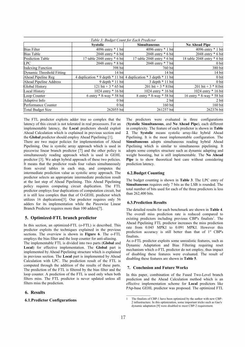
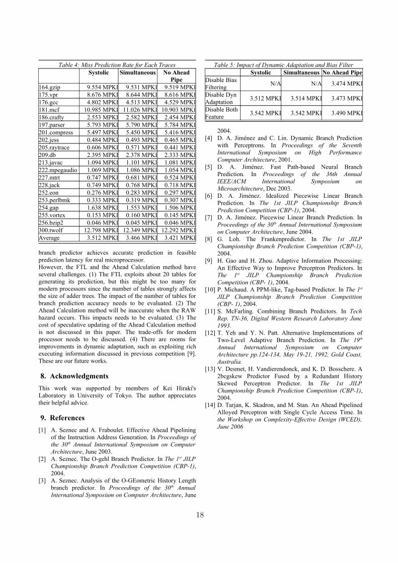
– Fused Two-Level Branch Prediction with Ahead CalculationYasuo Ishii(NEC Corporation, Computer Division)

• Selection of the Winner of the Realistic Track (9:55am)

• Coffee Break (10:00am)

• Session 2: Idealistic Track (10:30am)– PMPM: Prediction by Combining Multiple Partial Matches

(This finalist competes in both tracks)Hongliang Gao(School of Electrical Engineering and Computer Science, Universityof Central Florida)Huiyang Zhou(School of Electrical Engineering and Computer Science, Universityof Central Florida)

– Looking for Limits in Branch Prediction with the GTL Predict orAndre Seznec(IRISA/INRIA/HiPEAC)

– Neuro-PPM Branch PredictionRam Srinivasan(CCS-3 Modeling, Algorithms and Informatics, Los Alamos NationalLaboratory and Klipsch School of Electrical and Computer Engineering, New Mex-ico State University)Eitan Frachtenberg(CCS-3 Modeling, Algorithms and Informatics, Los Alamos Na-tional Laboratory)Olaf Lubeck(CCS-3 Modeling, Algorithms and Informatics, Los Alamos NationalLaboratory)Scott Pakin(CCS-3 Modeling, Algorithms and Informatics, Los Alamos NationalLaboratory)Jeanine Cook(Klipsch School of Electrical and Computer Engineering, New MexicoState University)

• Selection of the Winner of the Idealistic Track and Future Directions(11:45am)

iv

A 256 Kbits L-TAGE branch predictor

Andre Seznec

IRISA/INRIA/HIPEAC

Abstract

The TAGE predictor, TAgged GEometric length predictor,

was introduced in [10].

TAGE relies on several predictor tables indexed through

independent functions of the global branch/path history and

the branch address. The TAGE predictor uses (partially)

tagged components as the PPM-like predictor [5]. It relies

on (partial) match as the prediction computation function.

TAGE also uses GEometric history length as the O-GEHL

predictor [6], i.e. , the set of used global history lengths

forms a geometric series, i.e., . This al-

lows to efficiently capture correlation on recent branch out-

comes as well as on very old branches.

For the realistic track of CBP-2, we present a L-TAGE

predictor consisting of a 13-component TAGE predictor

combined with a 256-entry loop predictor. This predictor

achieves 3.314 misp/KI on the set of distributed traces.

Presentation outline

We first recall the TAGE predictor principles [10] and its

main characteristics. Then, we describe the L-TAGE con-

figuration submitted to CBP-2 combining a loop predictor

and a TAGE predictor. Section 3 discusses implementation

issues on the L-TAGE predictor. Section 4 presents simula-

tion results for the submitted L-TAGE predictor and a few

other TAGE predictor configurations. Section 5 briefly re-

views the related works that had major influences in the L-

TAGE predictor proposition and discusses a few tradeoffs

that might influence the choice of a TAGE configuration for

an effective implementation.

1. The TAGE conditional branch predictor

The TAGE predictor is derived from Michaud’s PPM-

like tag-based branch predictor [5] and uses geometric his-

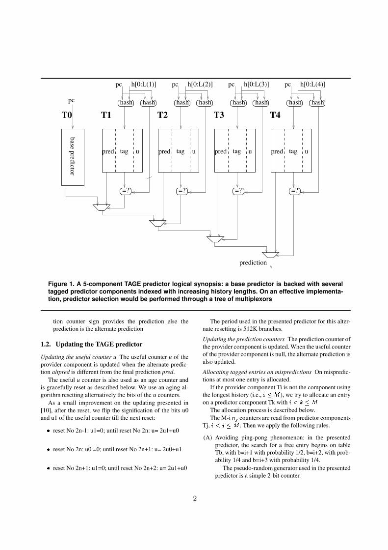
tory lengths [6]. Figure 1 illustrates a TAGE predictor. The

TAGE predictor features a base predictor T0 in charge of

providing a basic prediction and a set of (partially) tagged

This work was partially supported by an Intel research grant, an Intelresearch equipment donation and by the European Commission in the

context of the SARC integrated project #27648 (FP6).

predictor components Ti. These tagged predictor compo-

nents Ti, are indexed using different his-

tory lengths that form a geometric series, i.e,

.

Throughout this paper, the base predictor will be a sim-

ple PC-indexed 2-bit counter bimodal table; in order to save

storage space, the hysteresis bit is shared among several

counters as in [7].

An entry in a tagged component consists in a signed

counter ctr which sign provides the prediction, a (partial)

tag and an unsigned useful counter u. Throughout this pa-

per, u is a 2-bit counter and ctr is a 3-bit counter.

A few definitions and notations The provider component is

the matching component with the longest history. The al-

ternate prediction altpred is the prediction that would have

occurred if there had been a miss on the provider compo-

nent.

If there is no hitting component then altpred is the de-

fault prediction.

1.1. Prediction computation

At prediction time, the base predictor and the tagged

components are accessed simultaneously. The base predic-

tor provides a default prediction. The tagged components

provide a prediction only on a tag match.

In the general case, the overall prediction is provided by

the hitting tagged predictor component that uses the longest

history, or in case of no matching tagged predictor compo-

nent, the default prediction is used.

However, we found that, on several applications, using

the alternate prediction for newly allocated entries is more

efficient. Our experiments showed this property is essen-

tially global to the application and can be dynamicallymon-

itored through a single 4-bit counter (USE ALT ON NA in

the simulator). On the predictor an entry is classified as

“newly allocated” if its prediction counter is weak.

Therefore the prediction computation algorithm is as fol-

lows:

1. Find the matching component with the longest history

2. if (the prediction counter is not weak or

USE ALT ON NA is negative) then the predic-

1

h[0:L(4)]h[0:L(3)]h[0:L(2)]h[0:L(1)]

hash

=?

hash hash

=?

hash hash

=?

hash hash

=?

hash

tag u tag u pred tag u pred tag upred pred

prediction

pc pc pc pc

pc

base p

redicto

r

T0 T1 T2 T3 T4

Figure 1. A 5-component TAGE predictor logical synopsis: a base predictor is backed with several

tagged predictor components indexed with increasing history lengths. On an effective implementa-tion, predictor selection would be performed thrrough a tree of multiplexors

tion counter sign provides the prediction else the

prediction is the alternate prediction

1.2. Updating the TAGE predictor

Updating the useful counter u The useful counter u of the

provider component is updated when the alternate predic-

tion altpred is different from the final prediction pred.

The useful u counter is also used as an age counter and

is gracefully reset as described below. We use an aging al-

gorithm resetting alternatively the bits of the u counters.

As a small improvement on the updating presented in

[10], after the reset, we flip the signification of the bits u0

and u1 of the useful counter till the next reset:

reset No 2n-1: u1=0; until reset No 2n: u= 2u1+u0

reset No 2n: u0 =0; until reset No 2n+1: u= 2u0+u1

reset No 2n+1: u1=0; until reset No 2n+2: u= 2u1+u0

The period used in the presented predictor for this alter-

nate resetting is 512K branches.

Updating the prediction counters The prediction counter of

the provider component is updated.When the useful counter

of the provider component is null, the alternate prediction is

also updated.

Allocating tagged entries on mispredictions On mispredic-

tions at most one entry is allocated.

If the provider component Ti is not the component using

the longest history (i.e., ), we try to allocate an entry

on a predictor component Tk with

The allocation process is described below.

The M-i counters are read from predictor components

Tj, . Then we apply the following rules.

(A) Avoiding ping-pong phenomenon: in the presented

predictor, the search for a free entry begins on table

Tb, with b=i+1 with probability 1/2, b=i+2, with prob-

ability 1/4 and b=i+3 with probability 1/4.

The pseudo-randomgenerator used in the presented

predictor is a simple 2-bit counter.

2

(B) Initializing the allocated entry: An allocated entry is

initialized with the prediction counter set to weak cor-

rect. Counter u is initialized to 0 (i.e., strong not use-

ful).

2. Characteristics of the submitted L-TAGE

predictor

2.1. Information used for indexing the branch pre-dictor

2.1.1. Path and branch history The predictor compo-

nents are indexed using a hash function of the program

counter, the global branch history ghist (including non-

conditional branches as in [6]) and a (limited) 16-bit path

history phist consisting of 1 address bit per branch.

2.1.2. Discriminating kernel and user branchs Kernel

and user codes appear in the traces. In practice in the traces,

we were able to discrimate user code from kernal through

the address range. In order to avoid history pollution by ker-

nel code, we use two sets of histories: the user history is up-

dated only on user branches, kernel history is updated on all

branches.

2.2. Tag width tradeoff

Using a large tag width leads to waste part of the storage

while using a too small tag width leads to false tag match

detections. Experiments showed that one can use narrower

tags on the tables with smaller history lengths.

2.3. Number of the TAGE predictor components

For a 256 Kbits predictor, the best accuracy we found is

achieved by a 13 components TAGE predictor.

2.4. The submitted L-TAGE predictor

2.4.1. The loop predictor component The loop predictor

simply tries to identify regular loops with constant number

of iterations.

The loop predictor provides the global prediction when

the loop has successively been executed 3 times with the

same number of iterations. The loop predictor used in the

submission features 256 entries and is 4-way associative.

Each entry consists of a past iteration count on 14 bits, a

current iteration count on 14 bits, a partial tag on 14 bits, a

confidence counter on 2 bits and an age counter on 8 bits,

i.e. 52 bits per entry. The loop predictor storage is therefore

13 Kbits.

Replacement policy is based on the age. An entry can be

replaced only if its age counter is null. On allocation, age is

first set to 255. Age is decremented whenever the entry was

a possible replacement target and incremented when the en-

try is used and has provided a valid prediction. Age is re-

set to zero whenever the branch is determined as not being

a regular loop.

2.4.2. The TAGE predictor component The TAGE pre-

dictor features 12 tagged components and a base bimodal

predictor. Hysteresis bits are shared on the base predictor.

Each entry in predictor table Ti features a Wi bits wide tag,

a 3-bit prediction counter and a 2-bit useful counter.

The submitted predictor uses 4 as its minimum history

length and 640 as its maximum history length.

The characteristics of the TAGE component are summa-

rized in Table 1. The TAGE predictor features a total of

241.5 Kbits of prediction storage.

2.4.3. Total predictor storage budget Apart the predic-

tion table storage, the predictor uses two 640 bits global

history vectors, two 16 bits path history vectors, a 4 bits

USE ALT ON NA counter, a 19 bits counter for gracefully

resetting the u counters, a 2-bit counter as pseudo-random

generator and a 7-bit counter WITHLOOP to determine the

usefulness of the loop predictor. That is an extra storage of

1344 bits.

Therefore the predictor uses a total of (241.5+13)*1024

+ 1344 = 261,952 storage bits.

3. Implementation issues

3.1. The prediction response time

Since the loop predictor features a small number of en-

tries, the response time of the submitted predictor is domi-

nated by the TAGE response time.

The prediction response time on most global history

predictors involves three components: the index computa-

tion, the predictor table read and the prediction computa-

tion logic.

It was shown in [6] that very simple indexing functions

using a single stage of 3-entry exclusive-OR gates can be

used for indexing the predictor components without sig-

nificantly impairing the prediction accuracy. In the simula-

tion results presented in this paper, full hash functions were

used. However experiments using the 3-entry exclusive-OR

indexing functions described in [6] showed a very similar

total misprediction numbers (+0.03 misp/KI).

The predictor table read delay depends on the size of ta-

bles. On the TAGE predictor, the (partial) tags are needed

for the prediction computation. The tag computation may

span during the index computation and table read without

impacting the overall prediction computation time. Com-

plex hash functions may then be implemented.

The last stage in the prediction computation on the

TAGE predictor consists in the tag match followed by the

3

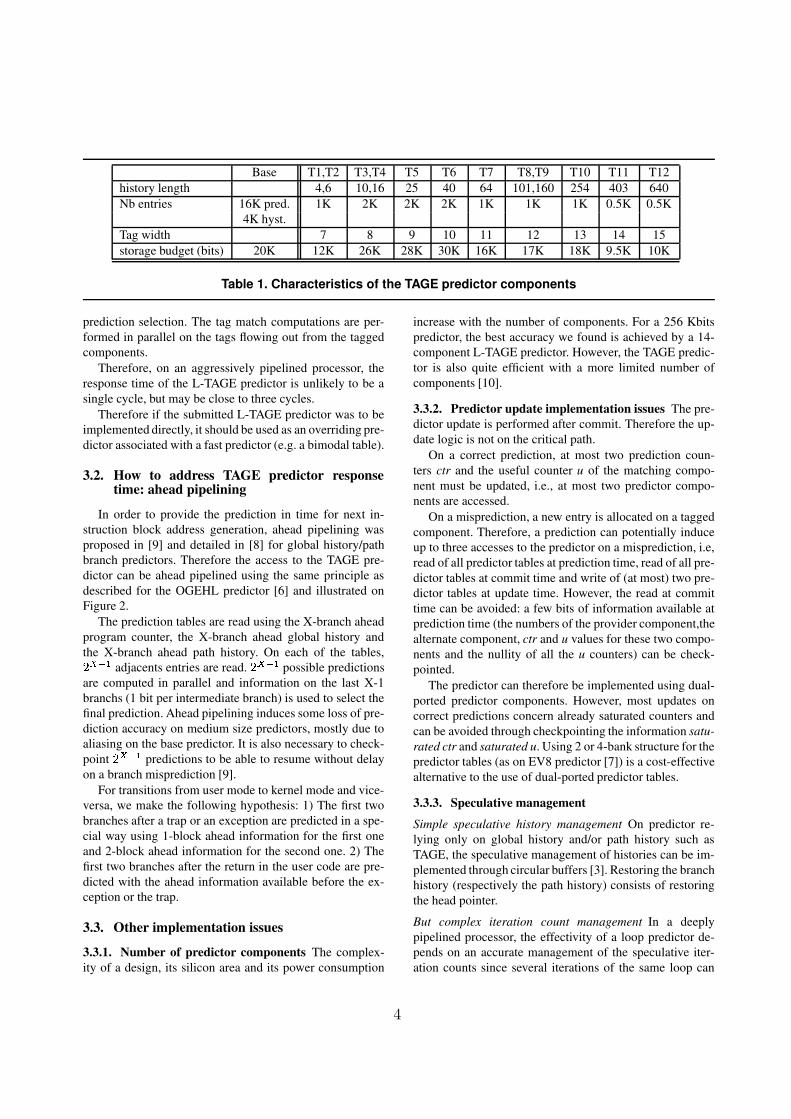
Base T1,T2 T3,T4 T5 T6 T7 T8,T9 T10 T11 T12

history length 4,6 10,16 25 40 64 101,160 254 403 640

Nb entries 16K pred. 1K 2K 2K 2K 1K 1K 1K 0.5K 0.5K

4K hyst.

Tag width 7 8 9 10 11 12 13 14 15

storage budget (bits) 20K 12K 26K 28K 30K 16K 17K 18K 9.5K 10K

Table 1. Characteristics of the TAGE predictor components

prediction selection. The tag match computations are per-

formed in parallel on the tags flowing out from the tagged

components.

Therefore, on an aggressively pipelined processor, the

response time of the L-TAGE predictor is unlikely to be a

single cycle, but may be close to three cycles.

Therefore if the submitted L-TAGE predictor was to be

implemented directly, it should be used as an overriding pre-

dictor associated with a fast predictor (e.g. a bimodal table).

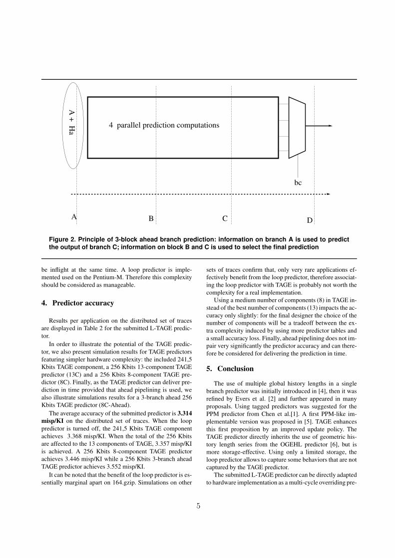
3.2. How to address TAGE predictor responsetime: ahead pipelining

In order to provide the prediction in time for next in-

struction block address generation, ahead pipelining was

proposed in [9] and detailed in [8] for global history/path

branch predictors. Therefore the access to the TAGE pre-

dictor can be ahead pipelined using the same principle as

described for the OGEHL predictor [6] and illustrated on

Figure 2.

The prediction tables are read using the X-branch ahead

program counter, the X-branch ahead global history and

the X-branch ahead path history. On each of the tables,

adjacents entries are read. possible predictions

are computed in parallel and information on the last X-1

branchs (1 bit per intermediate branch) is used to select the

final prediction. Ahead pipelining induces some loss of pre-

diction accuracy on medium size predictors, mostly due to

aliasing on the base predictor. It is also necessary to check-

point predictions to be able to resume without delay

on a branch misprediction [9].

For transitions from user mode to kernel mode and vice-

versa, we make the following hypothesis: 1) The first two

branches after a trap or an exception are predicted in a spe-

cial way using 1-block ahead information for the first one

and 2-block ahead information for the second one. 2) The

first two branches after the return in the user code are pre-

dicted with the ahead information available before the ex-

ception or the trap.

3.3. Other implementation issues

3.3.1. Number of predictor components The complex-

ity of a design, its silicon area and its power consumption

increase with the number of components. For a 256 Kbits

predictor, the best accuracy we found is achieved by a 14-

component L-TAGE predictor. However, the TAGE predic-

tor is also quite efficient with a more limited number of

components [10].

3.3.2. Predictor update implementation issues The pre-

dictor update is performed after commit. Therefore the up-

date logic is not on the critical path.

On a correct prediction, at most two prediction coun-

ters ctr and the useful counter u of the matching compo-

nent must be updated, i.e., at most two predictor compo-

nents are accessed.

On a misprediction, a new entry is allocated on a tagged

component. Therefore, a prediction can potentially induce

up to three accesses to the predictor on a misprediction, i.e,

read of all predictor tables at prediction time, read of all pre-

dictor tables at commit time and write of (at most) two pre-

dictor tables at update time. However, the read at commit

time can be avoided: a few bits of information available at

prediction time (the numbers of the provider component,the

alternate component, ctr and u values for these two compo-

nents and the nullity of all the u counters) can be check-

pointed.

The predictor can therefore be implemented using dual-

ported predictor components. However, most updates on

correct predictions concern already saturated counters and

can be avoided through checkpointing the information satu-

rated ctr and saturated u. Using 2 or 4-bank structure for the

predictor tables (as on EV8 predictor [7]) is a cost-effective

alternative to the use of dual-ported predictor tables.

3.3.3. Speculative management

Simple speculative history management On predictor re-

lying only on global history and/or path history such as

TAGE, the speculative management of histories can be im-

plemented through circular buffers [3]. Restoring the branch

history (respectively the path history) consists of restoring

the head pointer.

But complex iteration count management In a deeply

pipelined processor, the effectivity of a loop predictor de-

pends on an accurate management of the speculative iter-

ation counts since several iterations of the same loop can

4

A +

Ha

A B C D

4 parallel prediction computations

bc

Figure 2. Principle of 3-block ahead branch prediction: information on branch A is used to predict

the output of branch C; information on block B and C is used to select the final prediction

be inflight at the same time. A loop predictor is imple-

mented used on the Pentium-M. Therefore this complexity

should be considered as manageable.

4. Predictor accuracy

Results per application on the distributed set of traces

are displayed in Table 2 for the submitted L-TAGE predic-

tor.

In order to illustrate the potential of the TAGE predic-

tor, we also present simulation results for TAGE predictors

featuring simpler hardware complexity: the included 241,5

Kbits TAGE component, a 256 Kbits 13-component TAGE

predictor (13C) and a 256 Kbits 8-component TAGE pre-

dictor (8C). Finally, as the TAGE predictor can deliver pre-

diction in time provided that ahead pipelining is used, we

also illustrate simulations results for a 3-branch ahead 256

Kbits TAGE predictor (8C-Ahead).

The average accuracy of the submitted predictor is 3.314

misp/KI on the distributed set of traces. When the loop

predictor is turned off, the 241,5 Kbits TAGE component

achieves 3.368 misp/KI. When the total of the 256 Kbits

are affected to the 13 components of TAGE, 3.357 misp/KI

is achieved. A 256 Kbits 8-component TAGE predictor

achieves 3.446 misp/KI while a 256 Kbits 3-branch ahead

TAGE predictor achieves 3.552 misp/KI.

It can be noted that the benefit of the loop predictor is es-

sentially marginal apart on 164.gzip. Simulations on other

sets of traces confirm that, only very rare applications ef-

fectively benefit from the loop predictor, therefore associat-

ing the loop predictor with TAGE is probably not worth the

complexity for a real implementation.

Using a medium number of components (8) in TAGE in-

stead of the best number of components (13) impacts the ac-

curacy only slightly: for the final designer the choice of the

number of components will be a tradeoff between the ex-

tra complexity induced by using more predictor tables and

a small accuracy loss. Finally, ahead pipelining does not im-

pair very significantly the predictor accuracy and can there-

fore be considered for delivering the prediction in time.

5. Conclusion

The use of multiple global history lengths in a single

branch predictor was initially introduced in [4], then it was

refined by Evers et al. [2] and further appeared in many

proposals. Using tagged predictors was suggested for the

PPM predictor from Chen et al.[1]. A first PPM-like im-

plementable version was proposed in [5]. TAGE enhances

this first proposition by an improved update policy. The

TAGE predictor directly inherits the use of geometric his-

tory length series from the OGEHL predictor [6], but is

more storage-effective. Using only a limited storage, the

loop predictor allows to capture some behaviors that are not

captured by the TAGE predictor.

The submitted L-TAGE predictor can be directly adapted

to hardware implementation as a multi-cycle overriding pre-

5

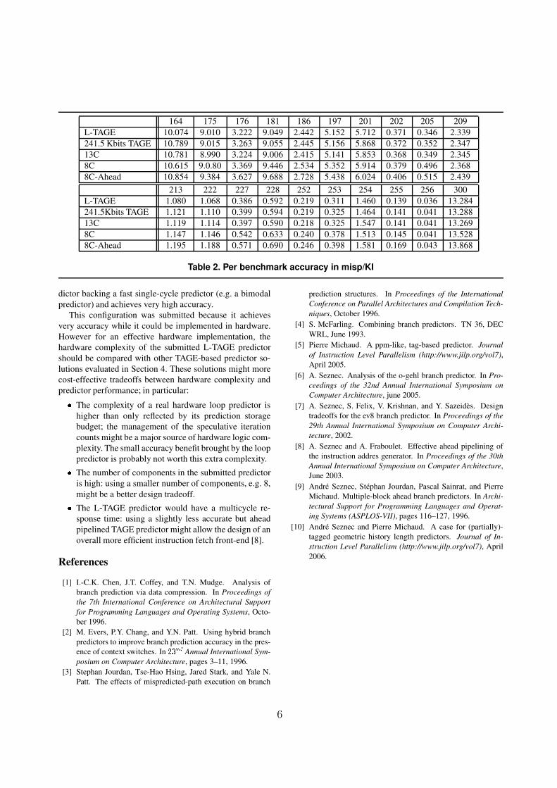
164 175 176 181 186 197 201 202 205 209

L-TAGE 10.074 9.010 3.222 9.049 2.442 5.152 5.712 0.371 0.346 2.339

241.5 Kbits TAGE 10.789 9.015 3.263 9.055 2.445 5.156 5.868 0.372 0.352 2.347

13C 10.781 8.990 3.224 9.006 2.415 5.141 5.853 0.368 0.349 2.345

8C 10.615 9.0.80 3.369 9.446 2.534 5.352 5.914 0.379 0.496 2.368

8C-Ahead 10.854 9.384 3.627 9.688 2.728 5.438 6.024 0.406 0.515 2.439

213 222 227 228 252 253 254 255 256 300

L-TAGE 1.080 1.068 0.386 0.592 0.219 0.311 1.460 0.139 0.036 13.284

241.5Kbits TAGE 1.121 1.110 0.399 0.594 0.219 0.325 1.464 0.141 0.041 13.288

13C 1.119 1.114 0.397 0.590 0.218 0.325 1.547 0.141 0.041 13.269

8C 1.147 1.146 0.542 0.633 0.240 0.378 1.513 0.145 0.041 13.528

8C-Ahead 1.195 1.188 0.571 0.690 0.246 0.398 1.581 0.169 0.043 13.868

Table 2. Per benchmark accuracy in misp/KI

dictor backing a fast single-cycle predictor (e.g. a bimodal

predictor) and achieves very high accuracy.

This configuration was submitted because it achieves

very accuracy while it could be implemented in hardware.

However for an effective hardware implementation, the

hardware complexity of the submitted L-TAGE predictor

should be compared with other TAGE-based predictor so-

lutions evaluated in Section 4. These solutions might more

cost-effective tradeoffs between hardware complexity and

predictor performance; in particular:

The complexity of a real hardware loop predictor is

higher than only reflected by its prediction storage

budget; the management of the speculative iteration

counts might be a major source of hardware logic com-

plexity. The small accuracy benefit brought by the loop

predictor is probably not worth this extra complexity.

The number of components in the submitted predictor

is high: using a smaller number of components, e.g. 8,

might be a better design tradeoff.

The L-TAGE predictor would have a multicycle re-

sponse time: using a slightly less accurate but ahead

pipelined TAGE predictor might allow the design of an

overall more efficient instruction fetch front-end [8].

References

[1] I.-C.K. Chen, J.T. Coffey, and T.N. Mudge. Analysis of

branch prediction via data compression. In Proceedings of

the 7th International Conference on Architectural Support

for Programming Languages and Operating Systems, Octo-

ber 1996.

[2] M. Evers, P.Y. Chang, and Y.N. Patt. Using hybrid branch

predictors to improve branch prediction accuracy in the pres-

ence of context switches. In Annual International Sym-

posium on Computer Architecture, pages 3–11, 1996.

[3] Stephan Jourdan, Tse-Hao Hsing, Jared Stark, and Yale N.

Patt. The effects of mispredicted-path execution on branch

prediction structures. In Proceedings of the International

Conference on Parallel Architectures and Compilation Tech-

niques, October 1996.

[4] S. McFarling. Combining branch predictors. TN 36, DEC

WRL, June 1993.

[5] Pierre Michaud. A ppm-like, tag-based predictor. Journal

of Instruction Level Parallelism (http://www.jilp.org/vol7),

April 2005.

[6] A. Seznec. Analysis of the o-gehl branch predictor. In Pro-

ceedings of the 32nd Annual International Symposium on

Computer Architecture, june 2005.

[7] A. Seznec, S. Felix, V. Krishnan, and Y. Sazeides. Design

tradeoffs for the ev8 branch predictor. In Proceedings of the

29th Annual International Symposium on Computer Archi-

tecture, 2002.

[8] A. Seznec and A. Fraboulet. Effective ahead pipelining of

the instruction addres generator. In Proceedings of the 30th

Annual International Symposium on Computer Architecture,

June 2003.

[9] Andre Seznec, Stephan Jourdan, Pascal Sainrat, and Pierre

Michaud. Multiple-block ahead branch predictors. In Archi-

tectural Support for Programming Languages and Operat-

ing Systems (ASPLOS-VII), pages 116–127, 1996.

[10] Andre Seznec and Pierre Michaud. A case for (partially)-

tagged geometric history length predictors. Journal of In-

struction Level Parallelism (http://www.jilp.org/vol7), April

2006.

6

Path Traced Perceptron Branch Predictor Using Local History

for Weight Selection

Yasuyuki Ninomiya and Koki Abe

Department of Computer Science

The University of Electro-Communications

1-5-1 Chofugaoka Chofu-shi

Tokyo 182-8585 Japan

{y-nino, abe}@cacao.cs.uec.ac.jp

Abstract

In this paper, we present a new perceptron branch pre-

dictor called Advanced Anti-Aliasing Perceptron Branch

Predictor (A3PBP), which can be reasonably implemented

as part of a modern micro-processor. Features of the predic-

tor are twofold: (1) Local history is used as part of the index

for weight tables; (2) Execution path history is effectively

used. Contrary to global/local perceptron branch predictor

where pipelining can not be realized, the scheme enables

accumulation of weights to be pipelined, and effectively re-

duces destructive aliasing, leading to increasing prediction

accuracy significantly. Compared with existing perceptron

branch predictors such as Piecewise Branch Predictor and

Path Trace Branch Predictor, our scheme requires less com-

putational costs than the former and utilizes execution path

history more efficiently than the latter. We present a ver-

sion of A3PBP where the number of pipeline stages is re-

duced as much as possible without increasing critical path

delay. The resulting predictor realizes a high prediction ac-

curacy. Discussions on implementability of the presented

predictor with respect to computational latency, memory re-

quirements, and computational costs are given.

1 Introduction

In recent years, central processing units tend to become

more deeply pipelined. The deeper the pipeline becomes,

the more the cycle time is reduced, but the more seriously

the performance can be degraded due to branch mispredic-

tion.

Perceptron branch predictors have extensively been stud-

ied these years to reduce the misprediction rate[6]. In

this paper, we propose a new perceptron branch predictor

called Advanced Anti-Aliasing Perceptron Branch Predic-

tor (A3PBP), which can be reasonably implemented as part

of a modern micro-processor. It is known that the behavior

of a branch is well predicted through learning its past be-

haviors with respect to the execution path history up to the

branch[3]. However, there is a possibility that a branch hav-

ing the same execution path history behaves differently in

some cases, and if it occurs the predictors solely based on

the path history fails to predict the outcome of the branch.

The phenomenon is called a destructive aliasing. In order

to resolve the destructive aliasing we propose to use the lo-

cal history of each branch on the execution path history. The

proposed scheme modifies the address of each branch on the

execution path history by substituting a part of the address

with its local history, and indexes the weight table by the

modified execution path history. By doing so, when predict-

ing the behavior of a branch, we can use individual weight

table entries on such occurrences that the execution paths

are the same but the modified execution paths are different,

resulting in resolving the destructive aliasing.

Contrary to the conventional global/local perceptron

branch predictor which can not be pipelined, the scheme

enables accumulation of weights to be pipelined. Com-

pared with existing perceptron branch predictors such as

Piecewise Branch Predictor[5] and Path Trace Branch

Predictor[2], our scheme requires less computational costs

than the former and utilizes execution history more effi-

ciently than the latter.

In this paper, we first describe recent studies on percep-

tron branch predictors, focusing on their methods of im-

provements and problems to be overcome. As a solution

to solve the problems A3PBP is proposed. A version of

A3PBP with reduced pipeline stages without increasing the

critical path delay are then described. Lastly, discussions on

implementability of the presented predictor with respect to

latency, memory requirements, and computational costs are

given.

7

2 Related Work

We refer to the current branch whose outcome is to be

predicted as “branch B” hereafter. Idealized Piecewise Lin-

ear Branch Predictor[4] uses the address of branch B as well

as the path, i.e., a dynamic sequence of branches leading to

B, as an index to access weight tables. It uses XOR of the

branch B address and the n-th older address within the path

as the index to access weights for the n-th global branch

history. The scheme reveals high prediction accuracy than

Global/Local[6] or Path-Based Neural Branch Predictor[3].

However, using the address of the current branch B as the

index to access every weight table does not allow to accu-

mulate the weights before the branch is fetched. The abil-

ity of accumulating the weights in advance is essential for

reducing the latency by pipelining. Thus Idealized Piece-

wise Linear Branch Predictor can not be pipelined with-

out exhausting in advance branches which will possibly be

fetched.

The problem was tried to be overcome by Ahead

Pipelined Piecewise Linear Branch Predictor[5] which uses

all possible values of reduced address of the branch B as

indices for accessing weight tables in upstream of pipeline

structure. However, it requires a large amount of compu-

tational cost to exhaust possible cases to occur, even if the

number of cases are reduced by limiting the width of the

branch B address.

Path Trace Branch Predictor (PTBP)[2] has a pipelined

structure with weight tables which are accessed in parallel.

A weight table in a stage is accessed by a hashed value of

addresses of branches at intervals of pipeline depth within

the path leading to the branch B. The scheme is motivated

by trying to utilize the path information as much as possible

within a pipelined structure. However, learning in PTBP

tends too sensitive to path history, resulting in a waste of

memory used by weight tables.

3 Advanced Anti-Aliasing Perceptron

Branch Predictor

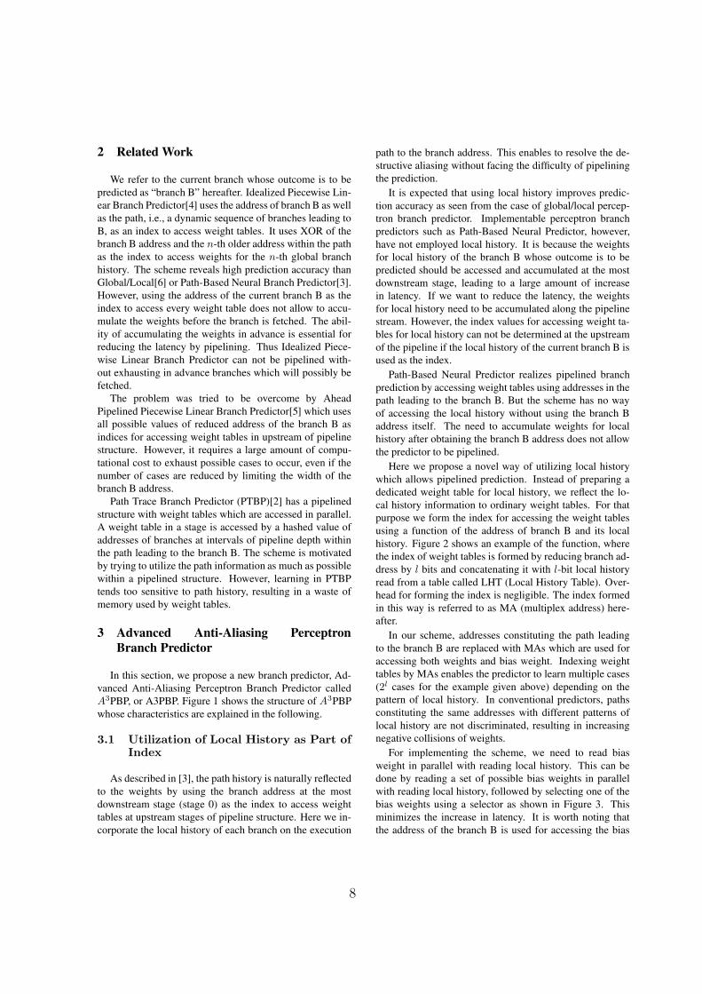
In this section, we propose a new branch predictor, Ad-

vanced Anti-Aliasing Perceptron Branch Predictor called

A3PBP, or A3PBP. Figure 1 shows the structure of A3PBP

whose characteristics are explained in the following.

3.1 Utilization of Local History as Part ofIndex

As described in [3], the path history is naturally reflected

to the weights by using the branch address at the most

downstream stage (stage 0) as the index to access weight

tables at upstream stages of pipeline structure. Here we in-

corporate the local history of each branch on the execution

path to the branch address. This enables to resolve the de-

structive aliasing without facing the difficulty of pipelining

the prediction.

It is expected that using local history improves predic-

tion accuracy as seen from the case of global/local percep-

tron branch predictor. Implementable perceptron branch

predictors such as Path-Based Neural Predictor, however,

have not employed local history. It is because the weights

for local history of the branch B whose outcome is to be

predicted should be accessed and accumulated at the most

downstream stage, leading to a large amount of increase

in latency. If we want to reduce the latency, the weights

for local history need to be accumulated along the pipeline

stream. However, the index values for accessing weight ta-

bles for local history can not be determined at the upstream

of the pipeline if the local history of the current branch B is

used as the index.

Path-Based Neural Predictor realizes pipelined branch

prediction by accessing weight tables using addresses in the

path leading to the branch B. But the scheme has no way

of accessing the local history without using the branch B

address itself. The need to accumulate weights for local

history after obtaining the branch B address does not allow

the predictor to be pipelined.

Here we propose a novel way of utilizing local history

which allows pipelined prediction. Instead of preparing a

dedicated weight table for local history, we reflect the lo-

cal history information to ordinary weight tables. For that

purpose we form the index for accessing the weight tables

using a function of the address of branch B and its local

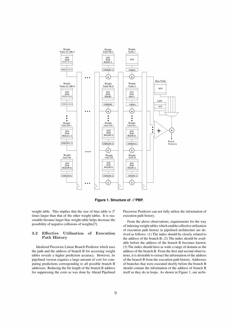
history. Figure 2 shows an example of the function, where

the index of weight tables is formed by reducing branch ad-

dress by l bits and concatenating it with l-bit local history

read from a table called LHT (Local History Table). Over-

head for forming the index is negligible. The index formed

in this way is referred to as MA (multiplex address) here-

after.

In our scheme, addresses constituting the path leading

to the branch B are replaced with MAs which are used for

accessing both weights and bias weight. Indexing weight

tables by MAs enables the predictor to learn multiple cases

(2l cases for the example given above) depending on the

pattern of local history. In conventional predictors, paths

constituting the same addresses with different patterns of

local history are not discriminated, resulting in increasing

negative collisions of weights.

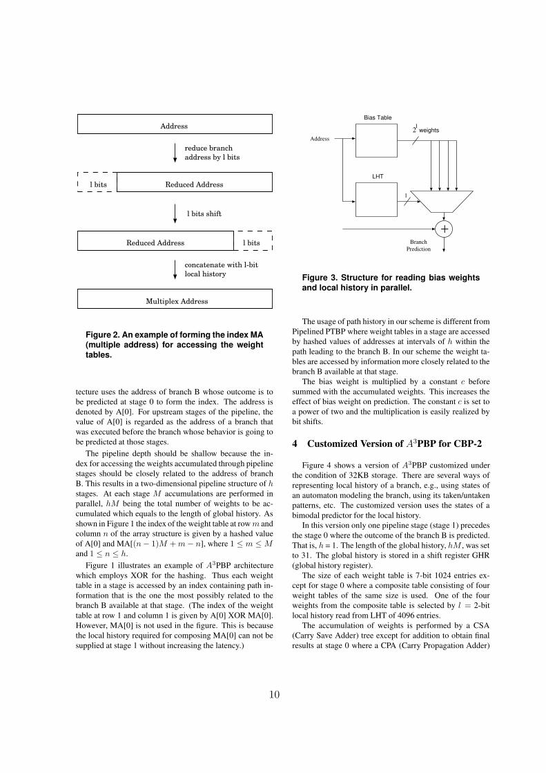
For implementing the scheme, we need to read bias

weight in parallel with reading local history. This can be

done by reading a set of possible bias weights in parallel

with reading local history, followed by selecting one of the

bias weights using a selector as shown in Figure 3. This

minimizes the increase in latency. It is worth noting that

the address of the branch B is used for accessing the bias

8

+

Table (h-1)M+1

A[0]XOR

MA[(M-1)(h-1)]

+

GHR[(M-1)(h-1)]

Branch

Prediction

Table (h-1)M+2

A[0]XOR

MA[hM-h-M+2]

GHR[hM-h-M+2]

A[0]XOR

MA[hM-h-1]

GHR[hM-h-1]

A[0]XOR

MA[hM-h]

GHR[hM-h]

Table 1

A[0]

GHR[0]

Table 2

A[0]

XOR

MA[1]

GHR[1]

A[0]XOR

MA[M-2]

GHR[M-2]

A[0]XOR

MA[M-1]

GHR[M-1]

+

+

+

+

Table hM-1

Table hM

Table M-1

Table M

Table M+1

GHR[M-1]

Table M+2

A[0]XOR

MA[M]

GHR[M]

A[0]XOR

MA[2M-3]

GHR[2M-3]

A[0]

XOR

MA[2M-2]

GHR[2M-2]

+

+

+

+

Table 2M-1

Table 2M

...

...

...

...

A[0]XOR

MA[M-1]

Weight Weight Weight

WeightWeightWeight

WeightWeightWeight

Weight Weight Weight

Bias Table

LHT

A[0]

A[0]

Figure 1. Structure of A3PBP.

weight table. This implies that the size of bias table is 2l

times larger than that of the other weight tables. It is rea-

sonable because larger bias weight table helps decrease the

possibility of negative collisions of weights[7].

3.2 Effective Utilization of ExecutionPath History

Idealized Piecewise Linear Branch Predictor which uses

the path and the address of branch B for accessing weight

tables reveals a higher prediction accuracy. However, its

pipelined version requires a large amount of cost for com-

puting predictions corresponding to all possible branch B

addresses. Reducing the bit length of the branch B address

for suppressing the costs as was done by Ahead Pipelined

Piecewise Predictor can not fully utilize the information of

execution path history.

From the above observations, requirements for the way

of indexing weight tables which enables effective utilization

of execution path history in pipelined architecture are de-

rived as follows: (1) The index should be closely related to

the address of the branch B; (2) The index should be avail-

able before the address of the branch B becomes known;

(3) The index should have as wide a range of domain as the

address of the branch B. From the first and second observa-

tions, it is desirable to extract the information of the address

of the branch B from the execution path history. Addresses

of branches that were executed shortly before the branch B

should contain the information of the address of branch B

itself as they do in loops. As shown in Figure 1, our archi-

9

Address

Reduced Address l bits

Multiplex Address

reduce branch

address by l bits

concatenate with l-bit

local history

Reduced Addressl bits

l bits shift

Figure 2. An example of forming the index MA(multiple address) for accessing the weight

tables.

tecture uses the address of branch B whose outcome is to

be predicted at stage 0 to form the index. The address is

denoted by A[0]. For upstream stages of the pipeline, the

value of A[0] is regarded as the address of a branch that

was executed before the branch whose behavior is going to

be predicted at those stages.

The pipeline depth should be shallow because the in-

dex for accessing the weights accumulated through pipeline

stages should be closely related to the address of branch

B. This results in a two-dimensional pipeline structure of h

stages. At each stage M accumulations are performed in

parallel, hM being the total number of weights to be ac-

cumulated which equals to the length of global history. As

shown in Figure 1 the index of the weight table at row m and

column n of the array structure is given by a hashed value

of A[0] and MA[(n − 1)M + m − n], where 1 ≤ m ≤ M

and 1 ≤ n ≤ h.

Figure 1 illustrates an example of A3PBP architecture

which employs XOR for the hashing. Thus each weight

table in a stage is accessed by an index containing path in-

formation that is the one the most possibly related to the

branch B available at that stage. (The index of the weight

table at row 1 and column 1 is given by A[0] XOR MA[0].

However, MA[0] is not used in the figure. This is because

the local history required for composing MA[0] can not be

supplied at stage 1 without increasing the latency.)

+

Bias Table

LHT

Branch

Prediction

weights

Address

l

2l

Figure 3. Structure for reading bias weights

and local history in parallel.

The usage of path history in our scheme is different from

Pipelined PTBP where weight tables in a stage are accessed

by hashed values of addresses at intervals of h within the

path leading to the branch B. In our scheme the weight ta-

bles are accessed by information more closely related to the

branch B available at that stage.

The bias weight is multiplied by a constant c before

summed with the accumulated weights. This increases the

effect of bias weight on prediction. The constant c is set to

a power of two and the multiplication is easily realized by

bit shifts.

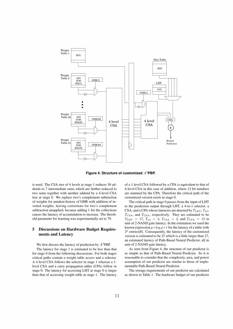
4 Customized Version of A3PBP for CBP-2

Figure 4 shows a version of A3PBP customized under

the condition of 32KB storage. There are several ways of

representing local history of a branch, e.g., using states of

an automaton modeling the branch, using its taken/untaken

patterns, etc. The customized version uses the states of a

bimodal predictor for the local history.

In this version only one pipeline stage (stage 1) precedes

the stage 0 where the outcome of the branch B is predicted.

That is, h = 1. The length of the global history, hM , was set

to 31. The global history is stored in a shift register GHR

(global history register).

The size of each weight table is 7-bit 1024 entries ex-

cept for stage 0 where a composite table consisting of four

weight tables of the same size is used. One of the four

weights from the composite table is selected by l = 2-bit

local history read from LHT of 4096 entries.

The accumulation of weights is performed by a CSA

(Carry Save Adder) tree except for addition to obtain final

results at stage 0 where a CPA (Carry Propagation Adder)

10

+

Branch

Prediction

Table 1A[0]

GHR[1]

Table 2 A[0]

XOR

MA[1]

GHR[1]

Weight

Bias Table

LHT

A[0]

A[0]

Weight

Table 30 A[0]

XOR

MA[29]

GHR[29]

Weight

Table 31 A[0]

XOR

MA[30]

GHR[30]

Weight

4 levelCSA

4 levelCSA

CSA

Figure 4. Structure of customized A3PBP.

is used. The CSA tree of 4 levels at stage 1 reduces 30 ad-

dends to 7 intermediate sums which are further reduced to

two sums together with another addend by a 4-level CSA

tree at stage 0. We replace two’s complement subtraction

of weights for untaken history of GHR with addition of in-

verted weights, leaving corrections for two’s complement

subtraction unapplied, because adding 1 for the collections

causes the latency of accumulation to increase. The thresh-

old parameter for learning was experimentally set to 79.

5 Discussions on Hardware Budget Require-

ments and Latency

We first discuss the latency of prediction by A3PBP.

The latency for stage 1 is estimated to be less than that

for stage 0 from the following discussions. For both stages

critical paths contain a weight table access and a selector.

A 4-level CSA follows the selector in stage 1 whereas a 1-

level CSA and a carry propagation adder (CPA) follow in

stage 0. The latency for accessing LHT at stage 0 is larger

than that of accessing weight table at stage 1. The latency

of a 1-level CSA followed by a CPA is equivalent to that of

4-level CSA in this case of addition, where 12 bit numbers

are summed by the CPA. Therefore the critical path of the

customized version exists in stage 0.

The critical path in stage 0 passes from the input of LHT

to the prediction output through LHT, a 4-to-1 selector, a

CSA, and a CPA whose latencies are denoted by TLHT, Tsel,

TCSA, and TCPA, respectively. They are estimated to be

TLHT = 17, Tsel = 4, TCSA = 4, and TCPA = 12 in

unit of 2-NAND gate latency. In the estimation we used the

known expression p+log p+1 for the latency of a table with

2p entries[8]. Consequently, the latency of the customized

version is estimated to be 37 which is a little larger than 27,

an estimated latency of Path-Based Neural Predictor, all in

unit of 2-NAND gate latency.

As seen from Figure 4, the structure of our predictor is

as simple as that of Path-Based Neural Predictor. So it is

reasonable to consider that the complexity, area, and power

assumption of our predictor are similar to those of imple-

mentable Path-Based Neural Predictor.

The storage requirements of our predictor are calculated

as shown in Table 1. The hardware budget of our predictor

11

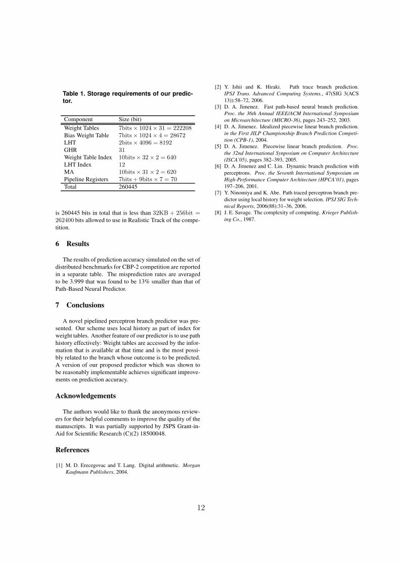
Table 1. Storage requirements of our predic-tor.

Component Size (bit)

Weight Tables 7bits × 1024 × 31 = 222208Bias Weight Table 7bits × 1024 × 4 = 28672LHT 2bits × 4096 = 8192GHR 31Weight Table Index 10bits × 32 × 2 = 640LHT Index 12MA 10bits × 31 × 2 = 620Pipeline Registers 7bits + 9bits × 7 = 70Total 260445

is 260445 bits in total that is less than 32KB + 256bit =262400 bits allowed to use in Realistic Track of the compe-

tition.

6 Results

The results of prediction accuracy simulated on the set of

distributed benchmarks for CBP-2 competition are reported

in a separate table. The misprediction rates are averaged

to be 3.999 that was found to be 13% smaller than that of

Path-Based Neural Predictor.

7 Conclusions

A novel pipelined perceptron branch predictor was pre-

sented. Our scheme uses local history as part of index for

weight tables. Another feature of our predictor is to use path

history effectively: Weight tables are accessed by the infor-

mation that is available at that time and is the most possi-

bly related to the branch whose outcome is to be predicted.

A version of our proposed predictor which was shown to

be reasonably implementable achieves significant improve-

ments on prediction accuracy.

Acknowledgements

The authors would like to thank the anonymous review-

ers for their helpful comments to improve the quality of the

manuscripts. It was partially supported by JSPS Grant-in-

Aid for Scientific Research (C)(2) 18500048.

References

[1] M. D. Erecegovac and T. Lang. Digital arithmetic. Morgan

Kaufmann Publishers, 2004.

[2] Y. Ishii and K. Hiraki. Path trace branch prediction.

IPSJ Trans. Advanced Computing Systems., 47(SIG 3(ACS

13)):58–72, 2006.

[3] D. A. Jimenez. Fast path-based neural branch prediction.

Proc. the 36th Annual IEEE/ACM International Symposium

on Microarchitecture (MICRO-36), pages 243–252, 2003.

[4] D. A. Jimenez. Idealized piecewise linear branch prediction.

in the First JILP Championship Branch Prediction Competi-

tion (CPB-1), 2004.

[5] D. A. Jimenez. Piecewise linear branch prediction. Proc.

the 32nd International Synposium on Computer Architecture

(ISCA’05), pages 382–393, 2005.

[6] D. A. Jimenez and C. Lin. Dynamic branch prediction with

perceptrons. Proc. the Seventh International Symposium on

High-Performance Computer Architecture (HPCA’01), pages

197–206, 2001.

[7] Y. Ninomiya and K. Abe. Path traced perceptron branch pre-

dictor using local history for weight selection. IPSJ SIG Tech-

nical Reports, 2006(88):31–36, 2006.

[8] J. E. Savage. The complexity of computing. Krieger Publish-

ing Co., 1987.

12

��

��

��

��

��

�� !"�!��!��

��

��

��

��

�� !� �� ! �"�� #��

$�� !�� #%$��

�� &��! � �� #%$��

�� &� � ��

��

�� !� � ��

��

��!��

��

��

�� &��! � �� ' � ��

#%$� � ��

��

��

�� (�)�� "��

��"��

�� (�)��

��!��!��

��*��+",��

��' � �� *��

��-�.//�)"0��,/,�.11�

��!��

��

��#��$��#�� #�� %�&��'�&��&�� ! ��

&��& � �� &�� (�� #��

#�� #� ��$�� $��&��$��

)�� * �� + �#�� ,�*+- � �%�&��# � &��&�

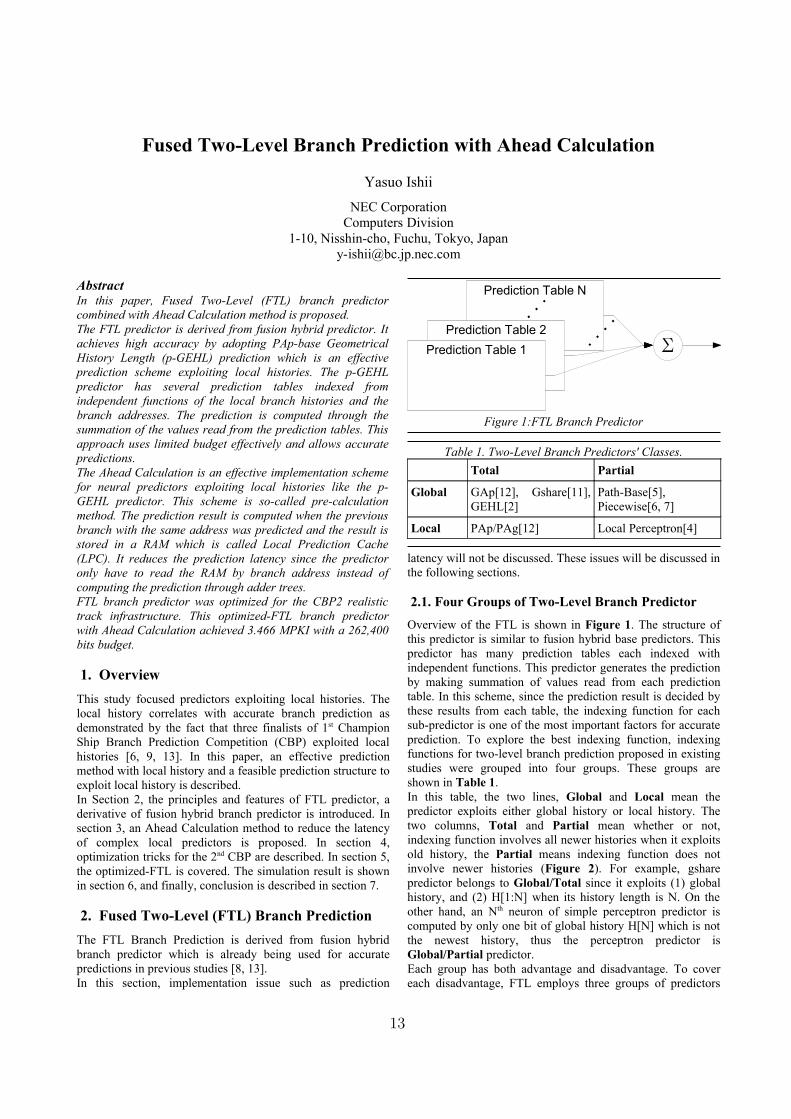
�� ./� � 0� � �12! � �� $$�� #��

��#�(��&��&�� #��$�� &�� #��

�%�&��&��&�� #�� #!

��)��3�� &��#�$�� $��4�� #��

#� ��$�$�� #� �� #�� #��#!��

��1��5��#��&��&��#�� #��&��

�$ � ��&�% � &��& � � �#�� #! � �� 6��

��7�� $� ��3�#��*+�� #�� #!��8��

��7�#��4�� #!��&�� &��(��

��/��#�$��&&��&��#�� #��9!

��

�� 4 �* �� + �#�� #� ��# � $ �� $�� #�

�� #�� (�� & ��#� � ��' � ��# � $� � ��

� �#�� #��.:��12!

�� &�� #��

&��(&&�� #��#!��(&&� ��#��#��

��$�&&�(�'��!

�� !��

;�� (��$��4��(�� "��!�� $�

�� #�� &� ��$�� #� �� #�� !��

� �#�� #�� &�� #�%�# � (��

�#��#��$��!�� #�� '�� #��

� ��' � �� $ ��&�� # � $ �� #��

�� &�!�� #�� &��#��#�#� ��

�� &��$ �� &��#�%�'�$��$� ��

�� #�� $�� $�� $� ��

� �#��! �� %�&� � � �� #�%�' � $�� #�%�'�

$��$� ��(��&��&� �� #�� #��%��'�

��#�� (� � � ' ��# � �� $�� ' ��! � �� ' ��

��(��# ��!

�� &�� (� � &�� #� � ��# ��

� �#�� %�&�� '&� �&�� &��& �� ! ��

�(� � ��&�� # �� (��

�#�%�'�$��&��&&��(� �� (��%�&��

�&# � �� #�%�' � $�� #��

��&�� (� � �� ,��"�� -! � �� %��&�� '��

� �#�� &��'�� #� $�� %�&��,�-�'&� �&�

�� #�,3-�<.�=2�(�� &��'��!�;��

�� #� �� $ ��&� �� #��

��#� ��&�� $�'&� �&�� <.2�(��

�� (�� #��

� #� $�� #�� !�

��' �� #��'��#�#��#��'�! ��

��#��#��'�� 4��&�� ' ��$ �� #��

�!��23 ��+��"��

��2��+��"��4��

��

� #� >5�.�32� � >�� .��2��

>�<4.32

+��*��.82��

+��(��./��92

�� +5�?+5'.�32 4��&�+� �� .62

��

��

��

13

$ �� #� $�� #� $�� # �� $�� ! � ��

��$��#�%�'��&��$�� ' ��

#�� #!

�� #� $��

��#�%�' �$�� $ �� #� $�� ' �� #� ��#�$ ��

>�<4�� #�� $�� #��

�$�� #� $�� #�� !�<�� &��'��$� �� #��

�� &��#�� #� ��'�� &�� 4,"-�@��"��

4,�-!��#�%�'�$��&��&��$� ��

��'��#�� &�� !�

�� #� $��

��#�%�'�$��$ �� #� $�� ' �� #� ��#�$ ��

>��A��#.02�(��%�&�� &�� $$��&�!��

�� #�%�' � $�� '�� ## �� $�

� �#�� &�� (��&&�� $�'&� �&�

�� !��&��'��$�� $�� !�

�� ' �� &�� %�&�� $� �� $� � ��

� �#��! � �� &�� #�� &�%�� $ � ��

� �#�� '�$��&�� #��'�� $��(�'��##� ��

�� #��&�� #�� !

��%�� $��

��*+�$��&��##��%�&��' ��!�<�(��

' ��&��$$�� #��!��

�#�%�'�$��$ �� $�� ' �� (��

>�<4�� #�� %��#�%�'�$��%�&��

&��& � �� ! �B� ��&& � �� +5�� >�<4� ,��

>�<4-�� #��!�� #�� &�� #��

�7� � �$ � �##� � � �� $ �� $��

�� #�� &�� &�� &�� &��&�

�� !

��& ��"�� "��'

�� #��&'� ��(��(��& ��#�� #��#��3!��

��#��#��'��&'� �� (��"��%!

�� $��' � ��# � � � ��&��# � � � �� ##� � � ��! � 5�

� �#�� &��#��#�#�$ ��'�� $��

�$��&�� #�$ �� #�� &��!��#� ��#�

$ ��$�� #�� #�� .:��12!��4��#��'��&��

� ��&��#� ��#�$ ��$�� #��#��'��&��! ��

��4�� #�� &��#��#�(�� #��

(�� &�� &�� $ � �� &&� � ��

�� &#�C!

�%� �� (��

�� 5��# � ��&��&�� # � $� ��

� �#�� #�� #��&��#�� #!

�%��)' �'��)��!��

D�#� �� #�� #��(�'�$��#��

#�� $�� #��&��#$$��&��$��

��&��&��$$��&�� !��&&��#$$��&��

$� �� #�� #��

�E� ��(��$� ��&��&�� &��#��

�� $� �� &�!��&��'�&�� $�&�$� �

�� $� ��! �� #� �� &��

��#� �� #�� &�� 5��#�

+��&��'!�<�(�� 5��#�+��&��'��#��

��&�#� $� �� #�� &��& �� &��

�� #��&�� #��#� �� #��#�#�

.�62! � �� &�� ( � ��&�� #�

��&&�#�5��#��&��&��#�� #!

�%�� "��'

�� 5��#��&��&��#��%�&��#!��

��E�� #�� #��&��$ �� #�� !�

�� #�� &��&�� %� �� #�� &� �(��

�� #�� #��!��&��&��#� ��&��$� ��

��%� � � �#�� # � � � � �F5D�(�� &&�# �4��&�

+ �#�� ,4+�-! � �� #�� %�&�� #�

��&��(�� #�� (��

1��+��"��3��!��

2��35�1

,��

-��35��6�7��&��$��

.��

8�� 1��

/��%��"��

1��9��:��3��!��;��3��

2��<5;��=>��=�?�@��

,��

-��;��5��'��

.��7��&��$��357��&��$��6�2

8��

/��7��&��$��357��&��$��2

A��

B��

C��

21�%��:��

�!��-3"��!��:��!��!��

1��+��D"��3��!��

2��35�1

,��

-��35��6�7��&��$��E�3F��

.��GH�%��&��

��$E��F�HG

8��

/�� 1��

A��%��D"��

1��+��"��D"��3��!��

2��35�1

,��

-��35��6�7��&��$��E��F��

.��GH�%�� &��

��$E��F�HG

8��

/�� 1��

A��%��"��D"��

�!��,3�%&��"��"��"��

14

�## ��! �� #�� (�� 5��# ��&��&�� &� ��

��#��4+��(�� #�� '�� !�� #��

&��&�� #�&��$�4+�!��

��&�� &�!��&��$$��&��&�� &�!�

5�� (��$��5��#��&��&��(��"��*!

�%�%��+��'��

�%�� &��$� �5��#��&��&��&��4+�!��7�#�

��4��4+��3�6:�� &��#�� 9�� :�

��!��&��#�� E� �� &��

#��&��$��'�&�'�!��4+��(��&��

F5D��&�� E� �� &��&��&&� ��#�&�(� ��(� �

��&�'��#��&��#��##� �

� ��!�� 4+��%��$� ��#� ��

� �� !

�%�*��,��!��-��.�/�� # � �$�� ( �� ,F5B- � ��7� # � ��' � ��

� �#�� (��5��#��&��&��!�<�(��

��$$��$��&&��7� #�� &��

(�� &��$�� #��$� ��

(�� $�( � ��&��! � )�� '�� &�� (&& � � � �� &&�# � ��

��7�#��#�� $&�� #� ��&�� !�� $��

�� (��&&��'�� #!

�*� ��0�

�� &�� #� � �(�#��E��$� ��

��7�#��4�� #�� #�� #!

�*�� "

��4��&�� $&�� '&�� #� ��!�

�� &� �� &7�#� �� A�A ��#�� #�%�#� ��

�## ��!�B�� #�� E� �#�� #�� #��

� �� (�� ## ��! �B�� &�� A�A � ��

� �#�� '�� #��&�� &��$��

��4�� #�� !�B�� #�� &��( ��'��

�� &�� E� �#�� #��#��#��#�� $�$&�� '�

� ��A�A��%��(�� #� ��&��7� �!��

� �#�� %�&�� #�� #� � ��&� �(��

��&�� #�$ �� $&�� '�� A�A!

�� &�� $�� &#� �� A�A�

�� '! �B�� &�� &&�

�� $ � �� (&& � �� A�A � �$�� %��

�(��! �� &#� �� (�� '��

�$$� �� !�� $�� &��&��&&�

��#� �� &�� # � ��

�� '�� $$� ! � <�(�� ' � ��# � ��

��&��# � � � �*+ � �$ ��

�� '�� $$� ��!��$��$&�� #��

�� $&�� '��#��$�� &�� &�

� �� !

�*��

�!��.3��

�

��

��

��

��

��

��

��

��

��

��

��

��

!��"��#��

$�# $�#

�� #�%��

$�#

��#�%�� &'�

$�#

�!��83%�� &��!

15

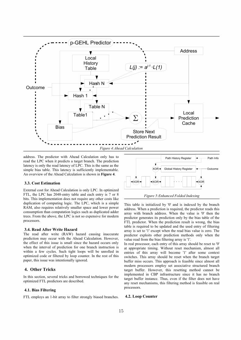
4�� &�� E�� (�#�$ ��>��A� � &��

��'��#�.02!�� #�&��

�� !�� $��&�� &��

�$� �� (�� $#�� &��! � �� &��

$�� &�� &�%�� $��

�� #� �� '�� $$� !��7�#��4�� #��

��&��:�(��&�� !

�*�%��+�� )��1��"

��4��%�&�� &��'�'&� �&�� &��'��>�<4�

� �#�� !��&�%��$$��#�%�'�� $� �

� #� �� #�� #�$�&#�#��#�%�'�� (��

��"��2�� #!��$�&#�#��#�%�'��#��

� ��#�� *+�.��2!��#�$�&#�#��#�%�'�

� ��%��#�#��&�#�� $�3� ��%�&��

� ��$�&#��$� ��!�5��&��$��

�#�%�'�$��$�� '�� #�� 3� ��%�&��

� �!�� &�� #�� #��

>�<4�� #�� !

�*�*��34��'�� "

G�#��'�� &#�C��'�$��&��$$�� $��

� �#�� (��#��'��&�� #� ��#�$ ��

� �#�� !�� &#�#$$� ��'� �� ! ��

��7�� &#��&��(��&��#��

&��'��$��'! ��$��'��&'� ��& ��#�� #�.32��

��# � � � � � � � �� $$�� #��'�! �B� �#��'� � � � �� 6� ��

�� !�

*�2��34��'��

�� $��&��$�� &��#�#��

�� &��'�� #��'! � �� #� � �&�� &�� &� �

#�� #�� '� � �%�&��' � �� %��

�$� ��=�� $�� $&�� #��&��

��#�� $��#��&� ��!

�� '�� $� � ��&��

� �#�� (�� &�� &��# �(�� #�� #��

#�� &�#!

�*�5�� "�!�� #� ��

�!��/3;��*�� +��"��

��

�� (��%��

��

��

)

��

��*��

��#��

*��&��"*��

��+��

#�%��

��

*��&��"��

�� (��%��(��%��

*��

��

��*��%#��

��

,-$

��

*��

��,3��!��%��"��

64�� 6�'� �� 7��

5��#�

+��&��'

)��&��

&�� #

)��&�� #�'�

�� #�� &�

5��#�

��&��&�� &� �� &� �� &�

*��

�&�� '�� &� �� &� �� &�

��#�%�'�

�� &� �� &� �� &�

��

�� &� �� &� �� &�

��

5#��'�� &� �� &� �� &�

B�'��

*��'�� &� �� &� �� &�

16

�� 4�� #�� %�&�� ##� � � �� &�% � ��

&��$�� &� ��#�� &�� !��

��&�� &� � &�� #�� &# � �%�&��

5��#��&��&��(��%�&��#�� #�

�� #� �� #�� &#��&��5��#�+��&��'�.�2!

�� (� ��"� ��&�� $� � ��&�� $ �5��#�

+��&��'! �;�� &� �� (�� #� ��

��(��&�� #�� .92��#�� &��

��&��&� � ��#�' � �� (�� # � � � >�<4�

� �#�� .12!�B��#�� #�� $��(��&��!�

�� #�� #��$�� &��&��&��

$ �� & � �� &�� # � ��

�� #�� #��&��&�� !��

� �#�� &�� #�� #�� &��

�� &�� $ �5��#�+��&��'! �� 5��#�+��&��'�

��&�� E� �� ' � � �� #��&��! � �� 4�

� �#�� &��$�� #��&��$��

��&&�&��&�%��$�;�>�<4�� #�� (��

��&7�� / � #��&��.12! �;� � � �#�� E� �� &� � 8/�

�##� � � $� � �� &�� (�&� � �� +��(�� 4��

* ��+ �#�� E� �� ##� �.92!

�2� � ��'�/��#��

��7�#��4�,��4-��#�� #!��

� �#�� %�&�� E�� %�&��# � � � ��

��! �� ( � � � ��(� � � ��"�� 5! � �� 4�

��&�� $&�� #��&�� $� ��&��'!

��&�� &��4��#�#�#��(�� ,� #� ��#�

�� - � $� � �$$�� &��!� �� #� � ��

��&��#� ��5��#�+��&��'�� (��%�&��#�

�� !�� &��#� ��5��#�

��&��&�� (�� 4+�! �� #�� &� � �$ � �� 4� ��

��#� �� '��##��$� �� &�� $� �� !�

�� #��$��4��$&�� #� �� $&�� #��

&�� !�5�� #��$��4��#��&��(��

$&�� ! �� 4�� #�� #��# ��&�� &&�

$&�� #��!

�5� ,��

�5��!�"��

�� #�� (� � � ��&��# � � � �� $'� ��

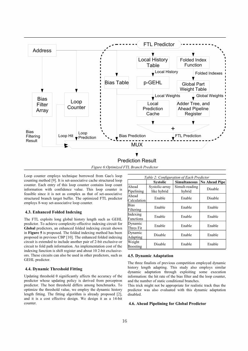
,64�� 6�'� ��#�7�� -��#$$� ��

��&�%��!��$�� $�� #�� (��# ��

�! � �� 64�� &� � � ��&�� # � 5��#�

+��&��'! � �� &�� &� ��$'� ��! ��

6�'� �� #�� &�� #�' � �� # � 5��#�

+��&��' � (�� &� � �� &�� &��'! � ��

�#��&�%�� #��#��'��#�

(�'�� '� � �� && � ��&�� &�! �� 7��

�� ( � �� & � �� (�� #� �'�

� �#��&��!

�5��"��"

�� #'��'��(�� # ��%!��4+�� $�

6�'� �� E� ��&��9� ��4)*�� #�#!��

��&�� $� ��#�$� ��$�� #�� &��

��3/3�6�� !

�5�%��,��

��#��&�#� ��&��$� �� (��# ��*!�

�� && � �� #�� #��# � �� # � ��

�%��' � � �#�� &�#�' � � �� *+A� � $��&��! � ��

5��#�+��&��'��4�� #�� #��

�� $ �� !�68 � D+H� � �� !�0� � D+H�! � <�(��

� �#�� && � �� $ � �� *+A��

$��&��!

5��4�� #�� %�&�� &��$��

�� 5#�� # � *�� &�� ' � �E� �' � ��

��(��4�� #�� #��&��

�$ � #�� &�' � �� $�� (� � � ��&��#! � �� &� � �$�

#�� &�'��$�� (��# ��2!

�8� �� -�0�

�� $ � �� # ��(��4��& � ��

� �#�� # � �� 5��# ��&��&�� # �(��

�$$�� &�� $� �� #�� &��

+5�� >�<4�� #�� (�� #!��7�#��4�

� ��$��&��$��*+�� 7�#� �� (��(��*+�

3��$ �� !��7�� >��A��

#��#��.02�(� ��#�� &�#��*+�3� �E� ��!

��-3�+��!��%��"��

64�� 6�'� �� 7��

*��&�� 6�0/�� I�� 6�0/�� I�� 6�0/�� I��

*�� &� 3�6:�� I�/� � 3�6:�� I�/� � 3�6:�� I�/� �

+ �#�� &� �9�� &��3�6:�� I�/� � �9�� &��3�6:�� I�/� � �:�� &��3�6:�� I�/� �

4+� 3�6:�� I�:� � 3�6:�� I�9� � ��

��#�%�'�� 10:� � 9/�� 1:��

�� &#��' �6� � �6� � �6� �

5��#�+��&��F�' 6�#��&��I�0�#��I�� 6�#��&��I�1�#��I��

5��#�+��&��5## �� 0�#��I�� 1�#��I��

>&� �&�<�� 3�� J�1�I�/8� � 3�� J�1�I�:� � 3�� J�1�I�:� �

4��&�<�� 36�� I��/� � ��36�� I��/� � ��36�� I��/� �

4�� /�� I�:�(��I�8:� � :�� I�:�(��I�8:� � �/�� I�:�(��I�8:� �

5#��$� �� 3� � 3� �

+� $� �� /�� /��

��&�*�#'��)7� 3/3�88� � 3/�389� � 3/319/� �

17

�� #�� #�� $�� &��

� �#��&��$� � ��&�� !

<�(�� 4��#� ��5��#��&��&��#��

�� &��&&��'��!�,�-��4��%�&�� 3�� &��$� �

'�� ' � �� #�� '�� $� �

��#� �� $�� &�� '&��$$��

��7��$��##� �� !��$�� $�� &��$� �

�� #�� #� � �� &��#! � ,3- ��

5��#��&��&��#�(&&� �� (��F5B�

��7� #�� ! �� #�� &��#! � ,1- ��

��$��&��#��'��$��5��#��&��&��#�

� � �� #��# � � � �� ! � �� #��$$� � $� ��#� ��

� �� #� � �� #��#! � ,6- � �� $� �

�� #��#��%�&��'� ��

�%��'��$� ��#��#�� .02!�

�� $�� (� ��!

�9� ��0�� "'��

�� (� � � (�� # � � � �� $ � H� � < ��A��

4� � �� G�� $ ��! ��

�� &�$�&��#��!

�:� ,�!��

.�2 5!�)�7��#�5!�� &��!��$$��5��#�+��&��'�

�$�� 5## ��>�� !��"��!��

��-1�� > ��

��3��1!

.32 5!�)�7��!��;�'��&�* ��+ �#�� !��2��I��"�

��+��"��+"�2��

3��6!

.12 5!�)�7��!�5��&��$��;�>�� <�� 4��'��

�� #�� ! � �� "��!� � �� -1��

��> ��

3��6!

.62 �!�5!��K��7��#��!�4�!��* ��+ �#��

(�� +� �� ! �� "��!� � �� >��

�� > �� $�!� � "��

��3��!

.82 �! � 5! � ��K��7! � �� +�� # � �� & � * ��

+ �#��! � �� "��!� � �� -/��

�%%%G��) � �� > ��

)��3��1!

./2 �! � 5! � ��K��7! � �#��&7�# � +��(�� 4�� * ��

+ �#��! �� 2�� I��" � �� +��

"��+"�2��3��6!

.92 �! �5!��K��7! �+��(�� 4�� * ��+ �#��! ��

"��!��-1��> ��

��3��6!

.:2 >! � 4��! � �� #�� ! � �� 2�� I��"�

��+��"��+"�2��

3��6!

.02 <!�>��#�<!�L��!�5#��$� ��+ ��'=�

5��$$��B�� +� �� + �#�� !��

�� 2�� I��" � �� +�� "��

��+"��2��3��6!

.��2 +!�D��#!�5�++D�&��'� ��#�+ �#�� !��2��

I��" � �� +�� "��

��+"��2��3��6!

.��2 )! �D�� &�'! � �� ' � * �� + �#�� ! � ��

(��J�-/��K�!��7��(�� I��

2CC-�

.�32 �!��#��! �!�+��! �5&�� &�� $�

�(��4��& � 5#�� * �� + �#��! � �� 2C��

�� > ��

��2,.�2-.��) �2C�,2��2CC,��#��

��

.�12 M!��<!�M��#� ��#��#�H!��!�*�� !�5�

3 �'��( � + �#�� # � � � � � F�#��#�� <��

)��(�# � +� �� + �#�� ! � �� 2�� I��"�

��+��"��+"�2��

3��6!

.�62 �!�� "��H!�)��# ��#�D!�)��!�5��5��#�+��&��#�

5&&��#�+� �� (��)�'&��&��5��!��

��7��'��&�� %��K��!��7�%K��

I��,11/

��83��K ��+��

64�� 6�'� �� 7��

�� &��*��

�&�� '?5 ?5 1!696�D+H�

�� &��

5#��1!8�3�D+H� 1!8�6�D+H� 1!691�D+H�

�� &��*��

�� 1!863�D+H� 1!863�D+H� 1!60��D+H�

��.3�)��"��(��%��

64�� 6�'� �� 7��

��

�/6!'7� 0!886�D+H� 0!81��D+H� 0!8�0�D+H�

�98!�� :!/9/�D+H� :!/66�D+H� :!/�/�D+H�

�9/!'�� 6!:�3�D+H� 6!8�1�D+H� 6!830�D+H�

�:�!��$ ��!0:8�D+H� ��!�3/�D+H� ��!0�1�D+H�

�:/!� �$�� 3!881�D+H� 3!8:3�D+H� 3!686�D+H�

�09!�� 8!901�D+H� 8!90��D+H� 8!9:6�D+H�

3��!�� 8!609�D+H� 8!68��D+H� 8!6�/�D+H�

3�3!"�� !6:6�D+H� �!601�D+H� �!6/8�D+H�

3�8! �� !/�/�D+H� �!89��D+H� �!66��D+H�

3�0!# 3!108�D+H� 3!19:�D+H� 3!111�D+H�

3�1!"�� !�06�D+H� �!��D+H� �!�:��D+H�

333!��'��#� �!�/0�D+H� �!�:/�D+H� �!�86�D+H�

339!�� !969�D+H� �!/:��D+H� �!836�D+H�

33:!"�� !960�D+H� �!9/:�D+H� �!9�:�D+H�

383!�� !39/�D+H� �!3:1�D+H� �!309�D+H�

381!�� & �� !111�D+H� �!1�0�D+H� �!1�9�D+H�

386!'�� !/1:�D+H� �!881�D+H� �!8�/�D+H�

388!�� % �!�81�D+H� �!�/��D+H� �!�68�D+H�

38/! 7�3 �!�6/�D+H� �!�68�D+H� �!�6/�D+H�

1��!�(�&$ �3!90:�D+H� �3!160�D+H� �3!303�D+H�

5�� '� 1!8�3�D+H� 1!6//�D+H� 1!63��D+H�

18

Abstract�The PPM prediction algorithm has been well known

for its high prediction accuracy. Recent proposals of PPM-like

predictors confirm its effectiveness on branch prediction. In this

paper, we introduce a new branch prediction algorithm, named

Prediction by combining Multiple Partial Matches (PMPM). The

PMPM algorithm selectively combines multiple matches instead

of using the longest match as in PPM. We analyze the PPM and

PMPM algorithms and show why PMPM is capable of making

more accurate predictions than PPM.

Based on PMPM, we propose both an idealistic predictor to

push the limit of branch prediction accuracy and a realistic

predictor for practical implementation. The simulation results

show that the proposed PMPM predictors achieve higher

prediction accuracy than the existing PPM-like branch predictors

such as the TAGE predictor. In addition, we model the effect of

ahead pipelining on our implementation and the results show that

the accuracy loss is relatively small.

1. INTRODUCTION

iven its importance on high performance microprocessor

design, branch prediction has been extensively studied. As

analyzed in [1], [9], the prediction by partial matching (PPM)

algorithm [2], originally proposed for text compression, can

achieve very high prediction accuracy for conditional branches.

Recent studies of PPM-like predictors [13], [8] confirm the

effectiveness of PPM and show that PPM-like predictors

outperform many state-of-art branch predictors.

In this paper, we propose to improve PPM-like branch

predictors by combining multiple partial matches rather than

the longest partial match as used in the PPM algorithm. We first

examine why longest partial match may lead to suboptimal

prediction accuracy. We then propose a prediction algorithm to

selectively combine multiple partial matches (PMPM) with an

adder tree.

Based on the PMPM algorithm, we develop an idealistic

predictor which explores extremely long history to push the

limit on branch prediction accuracy and a realistic predictor for

practical implementation. The realistic design is based on

recently developed PPM-like TAGE branch predictors [13] and

it has similar hardware complexity compared to the TAGE

predictor. Besides exploiting correlation from various global

branch histories, our design enables efficient integration of

local history information. The experimental results show that

the proposed designs can achieve higher accuracy than TAGE

predictors. Finally, we implement ahead pipelining to evaluate

the impact of the access latency of the proposed PMPM

predictor and the results show that with ahead pipelining, our

design can provide a prediction every cycle with relatively

small accuracy loss.

The rest of this paper is organized as follows. In Section 2 we

study the PPM branch prediction algorithm and introduce the

PMPM algorithm. An idealistic PMPM predictor is presented

in Section 3. Section 4 describes our design of realistic PMPM

predictors. Finally, Section 5 concludes the paper.

2. PREDICTION BY COMBINING MULTIPLE PARTIAL MATCHES

2.1. PPM with the (Confident) Longest Match

In the PPM algorithm, the Markov model, which determines

the prediction, is updated based on input information. When

used for branch prediction, the Markov model keeps track of

branch history and uses the longest match to make a prediction.

The assumption behind the longest match is that the longer

history provides a more accurate context to determine the

branch behavior.

However, since branches exhibit non-stationary behavior,

partial context matches may not be sufficient to accurately

predict branch outcomes. To examine this effect, we

implemented a PPM-based branch predictor, in which the

global branch history is used as the context for each branch. We

assign a signed saturating prediction counter with the range [-4,

4] for each (branch address, history) pair. The prediction

counter is incremented if the branch outcome is taken and

decremented otherwise. When both of the branch address and

history are matched, the corresponding prediction counter is

used to make a prediction. When there are multiple history

matches for the same branch with different history lengths, the

prediction counter associated with the longest history is used.

In order to show that the longest match may not be the best

choice for branch prediction, we implemented another scheme,

in which the prediction counter with the longest-history match

is not always selected to make a prediction. Instead, we use the

prediction counter as a confidence measure of the potential

prediction. Only when the prediction counter is a non-zero

value, it can be selected to make a prediction. We call such a

scheme as PPM with the confident longest match. We simulate

both schemes, i.e., PPM with the longest match and PPM with

the confident longest match, and report the misprediction rate

reductions, measured in mispredictions per 1000 instructions

(MPKI), achieved by the confident longest match. The results

are shown in Figure 1. In this experiment, the maximum history

length is set as 40.

From Figure 1, we can see that the confidence-based PPM

has lower misprediction rates than the PPM scheme for all the

benchmarks except the benchmark vortex, which implies that

the longest match used in PPM may lead to suboptimal

PMPM: Prediction by Combining Multiple Partial Matches

Hongliang Gao Huiyang Zhou

School of Electrical Engineering and Computer Science

University of Central Florida

{hgao, zhou}@cs.ucf.edu

G

19

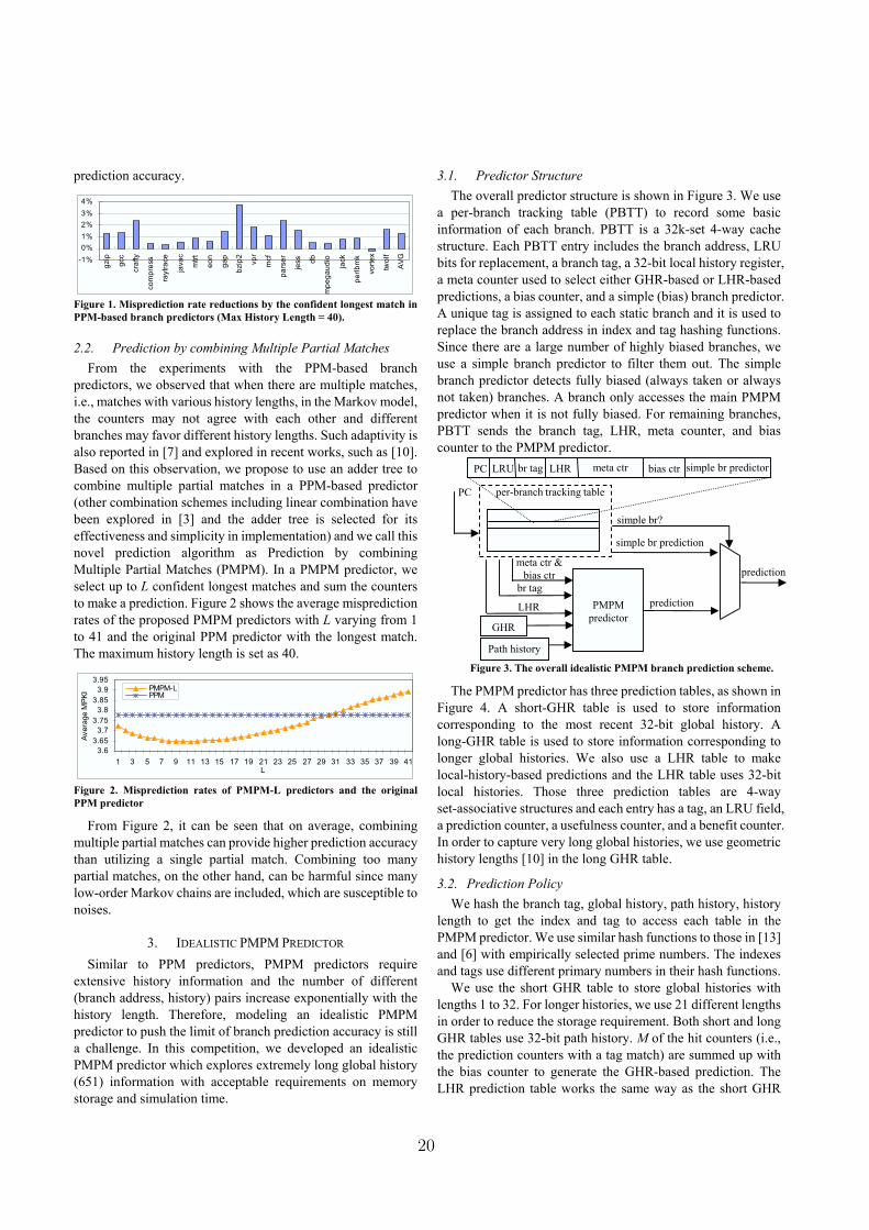
prediction accuracy.

-1%

0%

1%

2%

3%

4%

gzip

gcc

cra

fty

co

mp

ress

raytr

ace

java

c

mtr

t

eo

n

ga

p

bzip

2

vp

r

mcf

pa

rse

r

jess

db

mp

eg

au

dio

jack

pe

rlb

mk

vo

rte

x

two

lf

AV

G

Figure 1. Misprediction rate reductions by the confident longest match in

PPM-based branch predictors (Max History Length = 40).

2.2. Prediction by combining Multiple Partial Matches

From the experiments with the PPM-based branch

predictors, we observed that when there are multiple matches,

i.e., matches with various history lengths, in the Markov model,

the counters may not agree with each other and different

branches may favor different history lengths. Such adaptivity is

also reported in [7] and explored in recent works, such as [10].

Based on this observation, we propose to use an adder tree to

combine multiple partial matches in a PPM-based predictor

(other combination schemes including linear combination have

been explored in [3] and the adder tree is selected for its

effectiveness and simplicity in implementation) and we call this

novel prediction algorithm as Prediction by combining

Multiple Partial Matches (PMPM). In a PMPM predictor, we

select up to L confident longest matches and sum the counters

to make a prediction. Figure 2 shows the average misprediction

rates of the proposed PMPM predictors with L varying from 1

to 41 and the original PPM predictor with the longest match.

The maximum history length is set as 40.

3.6

3.65

3.7

3.75

3.8

3.85

3.9

3.95

1 3 5 7 9 11 13 15 17 19 21 23 25 27 29 31 33 35 37 39 41L

Avera

ge M

PK

I PMPM-LPPM

Figure 2. Misprediction rates of PMPM-L predictors and the original

PPM predictor

From Figure 2, it can be seen that on average, combining

multiple partial matches can provide higher prediction accuracy

than utilizing a single partial match. Combining too many

partial matches, on the other hand, can be harmful since many

low-order Markov chains are included, which are susceptible to

noises.

3. IDEALISTIC PMPM PREDICTOR

Similar to PPM predictors, PMPM predictors require

extensive history information and the number of different

(branch address, history) pairs increase exponentially with the

history length. Therefore, modeling an idealistic PMPM

predictor to push the limit of branch prediction accuracy is still

a challenge. In this competition, we developed an idealistic

PMPM predictor which explores extremely long global history

(651) information with acceptable requirements on memory

storage and simulation time.

3.1. Predictor Structure

The overall predictor structure is shown in Figure 3. We use

a per-branch tracking table (PBTT) to record some basic

information of each branch. PBTT is a 32k-set 4-way cache

structure. Each PBTT entry includes the branch address, LRU

bits for replacement, a branch tag, a 32-bit local history register,

a meta counter used to select either GHR-based or LHR-based

predictions, a bias counter, and a simple (bias) branch predictor.

A unique tag is assigned to each static branch and it is used to

replace the branch address in index and tag hashing functions.

Since there are a large number of highly biased branches, we

use a simple branch predictor to filter them out. The simple

branch predictor detects fully biased (always taken or always

not taken) branches. A branch only accesses the main PMPM

predictor when it is not fully biased. For remaining branches,

PBTT sends the branch tag, LHR, meta counter, and bias

counter to the PMPM predictor.

The PMPM predictor has three prediction tables, as shown in

Figure 4. A short-GHR table is used to store information

corresponding to the most recent 32-bit global history. A

long-GHR table is used to store information corresponding to

longer global histories. We also use a LHR table to make

local-history-based predictions and the LHR table uses 32-bit

local histories. Those three prediction tables are 4-way

set-associative structures and each entry has a tag, an LRU field,

a prediction counter, a usefulness counter, and a benefit counter.

In order to capture very long global histories, we use geometric

history lengths [10] in the long GHR table.

3.2. Prediction Policy

We hash the branch tag, global history, path history, history

length to get the index and tag to access each table in the

PMPM predictor. We use similar hash functions to those in [13]

and [6] with empirically selected prime numbers. The indexes

and tags use different primary numbers in their hash functions.

We use the short GHR table to store global histories with

lengths 1 to 32. For longer histories, we use 21 different lengths

in order to reduce the storage requirement. Both short and long

GHR tables use 32-bit path history. M of the hit counters (i.e.,

the prediction counters with a tag match) are summed up with

the bias counter to generate the GHR-based prediction. The

LHR prediction table works the same way as the short GHR

per-branch tracking table PC

PC br tag simple br predictorLRU

GHR

PMPM

predictor

simple br?

simple br prediction

prediction

prediction

Figure 3. The overall idealistic PMPM branch prediction scheme.

meta ctr

br tag

LHR

LHR bias ctr

meta ctr &

bias ctr

Path history

20

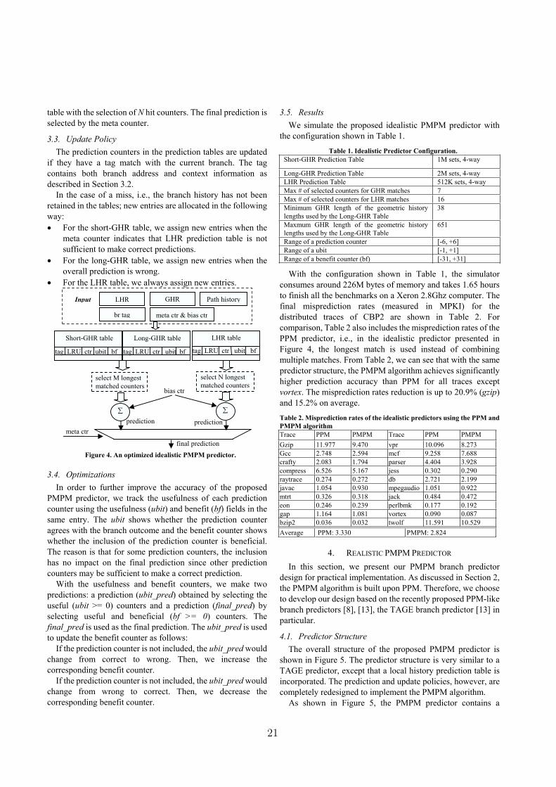
table with the selection of N hit counters. The final prediction is

selected by the meta counter.

3.3. Update Policy

The prediction counters in the prediction tables are updated

if they have a tag match with the current branch. The tag

contains both branch address and context information as

described in Section 3.2.

In the case of a miss, i.e., the branch history has not been

retained in the tables; new entries are allocated in the following

way:

For the short-GHR table, we assign new entries when the

meta counter indicates that LHR prediction table is not

sufficient to make correct predictions.

For the long-GHR table, we assign new entries when the

overall prediction is wrong.

For the LHR table, we always assign new entries.

3.4. Optimizations

In order to further improve the accuracy of the proposed

PMPM predictor, we track the usefulness of each prediction

counter using the usefulness (ubit) and benefit (bf) fields in the

same entry. The ubit shows whether the prediction counter

agrees with the branch outcome and the benefit counter shows

whether the inclusion of the prediction counter is beneficial.

The reason is that for some prediction counters, the inclusion

has no impact on the final prediction since other prediction

counters may be sufficient to make a correct prediction.

With the usefulness and benefit counters, we make two

predictions: a prediction (ubit_pred) obtained by selecting the

useful (ubit >= 0) counters and a prediction (final_pred) by

selecting useful and beneficial (bf >= 0) counters. The

final_pred is used as the final prediction. The ubit_pred is used

to update the benefit counter as follows:

If the prediction counter is not included, the ubit_pred would

change from correct to wrong. Then, we increase the

corresponding benefit counter.

If the prediction counter is not included, the ubit_pred would

change from wrong to correct. Then, we decrease the

corresponding benefit counter.

3.5. Results

We simulate the proposed idealistic PMPM predictor with

the configuration shown in Table 1.

Table 1. Idealistic Predictor Configuration.

Short-GHR Prediction Table 1M sets, 4-way

Long-GHR Prediction Table 2M sets, 4-way

LHR Prediction Table 512K sets, 4-way

Max # of selected counters for GHR matches 7

Max # of selected counters for LHR matches 16

Minimum GHR length of the geometric history

lengths used by the Long-GHR Table

38

Maxmum GHR length of the geometric history

lengths used by the Long-GHR Table

651

Range of a prediction counter [-6, +6]

Range of a ubit [-1, +1]

Range of a benefit counter (bf) [-31, +31]

With the configuration shown in Table 1, the simulator

consumes around 226M bytes of memory and takes 1.65 hours

to finish all the benchmarks on a Xeron 2.8Ghz computer. The

final misprediction rates (measured in MPKI) for the

distributed traces of CBP2 are shown in Table 2. For

comparison, Table 2 also includes the misprediction rates of the

PPM predictor, i.e., in the idealistic predictor presented in

Figure 4, the longest match is used instead of combining

multiple matches. From Table 2, we can see that with the same

predictor structure, the PMPM algorithm achieves significantly

higher prediction accuracy than PPM for all traces except

vortex. The misprediction rates reduction is up to 20.9% (gzip)

and 15.2% on average.

Table 2. Misprediction rates of the idealistic predictors using the PPM and

PMPM algorithm

Trace PPM PMPM Trace PPM PMPM

Gzip 11.977 9.470 vpr 10.096 8.273

Gcc 2.748 2.594 mcf 9.258 7.688

crafty 2.083 1.794 parser 4.404 3.928

compress 6.526 5.167 jess 0.302 0.290

raytrace 0.274 0.272 db 2.721 2.199

javac 1.054 0.930 mpegaudio 1.051 0.922

mtrt 0.326 0.318 jack 0.484 0.472

eon 0.246 0.239 perlbmk 0.177 0.192

gap 1.164 1.081 vortex 0.090 0.087

bzip2 0.036 0.032 twolf 11.591 10.529

Average PPM: 3.330 PMPM: 2.824

4. REALISTIC PMPM PREDICTOR

In this section, we present our PMPM branch predictor

design for practical implementation. As discussed in Section 2,

the PMPM algorithm is built upon PPM. Therefore, we choose

to develop our design based on the recently proposed PPM-like

branch predictors [8], [13], the TAGE branch predictor [13] in

particular.

4.1. Predictor Structure

The overall structure of the proposed PMPM predictor is

shown in Figure 5. The predictor structure is very similar to a

TAGE predictor, except that a local history prediction table is

incorporated. The prediction and update policies, however, are

completely redesigned to implement the PMPM algorithm.

As shown in Figure 5, the PMPM predictor contains a

Short-GHR table

prediction

tag LRU ctr ubit bf

br tag

LHR GHR Path historyInput

Long-GHR table

tag LRU ctr ubit bf

LHR table

tag LRU ctr ubit bf

select M longest

matched counters

select N longest

matched counters bias ctr

final prediction

meta ctr

meta ctr & bias ctr

prediction

Figure 4. An optimized idealistic PMPM predictor.

21

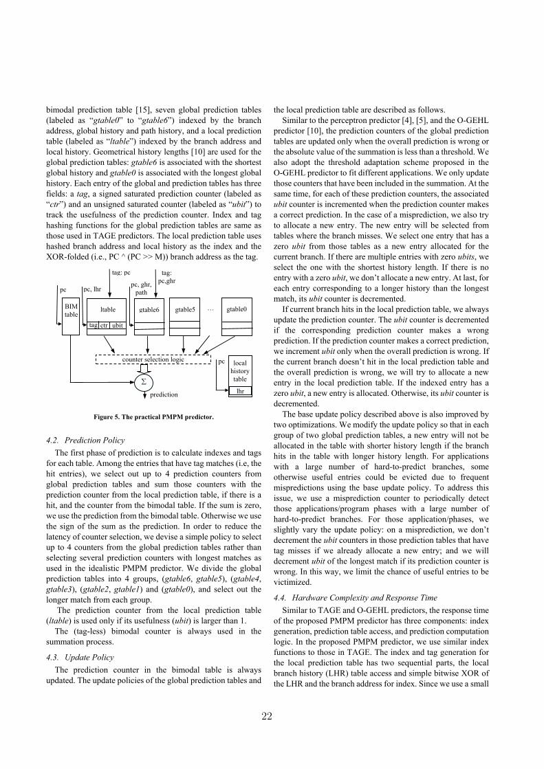
bimodal prediction table [15], seven global prediction tables

(labeled as �gtable0� to �gtable6�) indexed by the branch

address, global history and path history, and a local prediction

table (labeled as �ltable�) indexed by the branch address and

local history. Geometrical history lengths [10] are used for the

global prediction tables: gtable6 is associated with the shortest

global history and gtable0 is associated with the longest global

history. Each entry of the global and prediction tables has three

fields: a tag, a signed saturated prediction counter (labeled as

�ctr�) and an unsigned saturated counter (labeled as �ubit�) to

track the usefulness of the prediction counter. Index and tag

hashing functions for the global prediction tables are same as

those used in TAGE predictors. The local prediction table uses

hashed branch address and local history as the index and the

XOR-folded (i.e., PC ^ (PC >> M)) branch address as the tag.

Figure 5. The practical PMPM predictor.

4.2. Prediction Policy

The first phase of prediction is to calculate indexes and tags

for each table. Among the entries that have tag matches (i.e, the

hit entries), we select out up to 4 prediction counters from

global prediction tables and sum those counters with the

prediction counter from the local prediction table, if there is a

hit, and the counter from the bimodal table. If the sum is zero,

we use the prediction from the bimodal table. Otherwise we use

the sign of the sum as the prediction. In order to reduce the

latency of counter selection, we devise a simple policy to select

up to 4 counters from the global prediction tables rather than

selecting several prediction counters with longest matches as

used in the idealistic PMPM predictor. We divide the global

prediction tables into 4 groups, (gtable6, gtable5), (gtable4,

gtable3), (gtable2, gtable1) and (gtable0), and select out the

longer match from each group.

The prediction counter from the local prediction table

(ltable) is used only if its usefulness (ubit) is larger than 1.

The (tag-less) bimodal counter is always used in the

summation process.

4.3. Update Policy

The prediction counter in the bimodal table is always

updated. The update policies of the global prediction tables and

the local prediction table are described as follows.

Similar to the perceptron predictor [4], [5], and the O-GEHL

predictor [10], the prediction counters of the global prediction

tables are updated only when the overall prediction is wrong or

the absolute value of the summation is less than a threshold. We

also adopt the threshold adaptation scheme proposed in the

O-GEHL predictor to fit different applications. We only update

those counters that have been included in the summation. At the

same time, for each of these prediction counters, the associated

ubit counter is incremented when the prediction counter makes

a correct prediction. In the case of a misprediction, we also try

to allocate a new entry. The new entry will be selected from

tables where the branch misses. We select one entry that has a

zero ubit from those tables as a new entry allocated for the

current branch. If there are multiple entries with zero ubits, we

select the one with the shortest history length. If there is no

entry with a zero ubit, we don�t allocate a new entry. At last, for

each entry corresponding to a longer history than the longest

match, its ubit counter is decremented.

If current branch hits in the local prediction table, we always

update the prediction counter. The ubit counter is decremented

if the corresponding prediction counter makes a wrong

prediction. If the prediction counter makes a correct prediction,

we increment ubit only when the overall prediction is wrong. If

the current branch doesn�t hit in the local prediction table and

the overall prediction is wrong, we will try to allocate a new

entry in the local prediction table. If the indexed entry has a

zero ubit, a new entry is allocated. Otherwise, its ubit counter is

decremented.

The base update policy described above is also improved by

two optimizations. We modify the update policy so that in each

group of two global prediction tables, a new entry will not be

allocated in the table with shorter history length if the branch

hits in the table with longer history length. For applications

with a large number of hard-to-predict branches, some

otherwise useful entries could be evicted due to frequent

mispredictions using the base update policy. To address this

issue, we use a misprediction counter to periodically detect

those applications/program phases with a large number of

hard-to-predict branches. For those application/phases, we

slightly vary the update policy: on a misprediction, we don�t

decrement the ubit counters in those prediction tables that have

tag misses if we already allocate a new entry; and we will

decrement ubit of the longest match if its prediction counter is

wrong. In this way, we limit the chance of useful entries to be

victimized.

4.4. Hardware Complexity and Response Time

Similar to TAGE and O-GEHL predictors, the response time

of the proposed PMPM predictor has three components: index

generation, prediction table access, and prediction computation

logic. In the proposed PMPM predictor, we use similar index

functions to those in TAGE. The index and tag generation for

the local prediction table has two sequential parts, the local

branch history (LHR) table access and simple bitwise XOR of

the LHR and the branch address for index. Since we use a small

ltable

tag ctr ubit

counter selection logic

BIM

table

prediction

pc pc, lhr

tag: pc

local

history

table

pc

lhr

gtable6

pc, ghr,

path

tag:

pc,ghr

gtable5 gtable0�

22

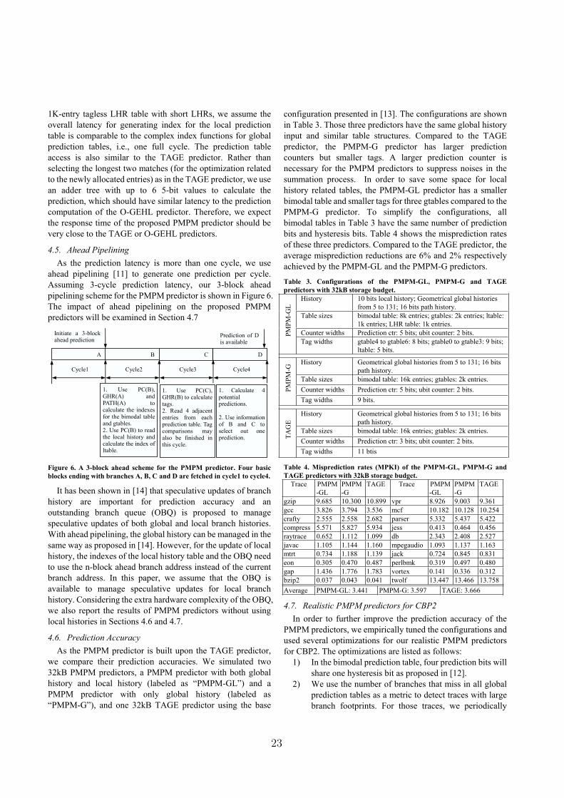
1K-entry tagless LHR table with short LHRs, we assume the

overall latency for generating index for the local prediction

table is comparable to the complex index functions for global

prediction tables, i.e., one full cycle. The prediction table

access is also similar to the TAGE predictor. Rather than

selecting the longest two matches (for the optimization related

to the newly allocated entries) as in the TAGE predictor, we use

an adder tree with up to 6 5-bit values to calculate the

prediction, which should have similar latency to the prediction

computation of the O-GEHL predictor. Therefore, we expect

the response time of the proposed PMPM predictor should be

very close to the TAGE or O-GEHL predictors.

4.5. Ahead Pipelining

As the prediction latency is more than one cycle, we use

ahead pipelining [11] to generate one prediction per cycle.

Assuming 3-cycle prediction latency, our 3-block ahead

pipelining scheme for the PMPM predictor is shown in Figure 6.

The impact of ahead pipelining on the proposed PMPM

predictors will be examined in Section 4.7

A B C D

1. Use PC(B), GHR(A) and PATH(A) to calculate the indexes for the bimodal table and gtables. 2. Use PC(B) to read the local history and calculate the index of ltable.

Initiate a 3-block ahead prediction

Prediction of D is available

1. Use PC(C), GHR(B) to calculate tags. 2. Read 4 adjacent entries from each prediction table. Tag comparisons may also be finished in this cycle.

1. Calculate 4 potential predictions.

2. Use information of B and C to select out one prediction.

Cycle1 Cycle2 Cycle3 Cycle4

Figure 6. A 3-block ahead scheme for the PMPM predictor. Four basic

blocks ending with branches A, B, C and D are fetched in cycle1 to cycle4.

It has been shown in [14] that speculative updates of branch

history are important for prediction accuracy and an

outstanding branch queue (OBQ) is proposed to manage

speculative updates of both global and local branch histories.

With ahead pipelining, the global history can be managed in the

same way as proposed in [14]. However, for the update of local

history, the indexes of the local history table and the OBQ need

to use the n-block ahead branch address instead of the current

branch address. In this paper, we assume that the OBQ is

available to manage speculative updates for local branch

history. Considering the extra hardware complexity of the OBQ,

we also report the results of PMPM predictors without using

local histories in Sections 4.6 and 4.7.

4.6. Prediction Accuracy

As the PMPM predictor is built upon the TAGE predictor,

we compare their prediction accuracies. We simulated two

32kB PMPM predictors, a PMPM predictor with both global

history and local history (labeled as �PMPM-GL�) and a

PMPM predictor with only global history (labeled as

�PMPM-G�), and one 32kB TAGE predictor using the base

configuration presented in [13]. The configurations are shown

in Table 3. Those three predictors have the same global history

input and similar table structures. Compared to the TAGE

predictor, the PMPM-G predictor has larger prediction

counters but smaller tags. A larger prediction counter is

necessary for the PMPM predictors to suppress noises in the

summation process. In order to save some space for local

history related tables, the PMPM-GL predictor has a smaller

bimodal table and smaller tags for three gtables compared to the

PMPM-G predictor. To simplify the configurations, all

bimodal tables in Table 3 have the same number of prediction

bits and hysteresis bits. Table 4 shows the misprediction rates

of these three predictors. Compared to the TAGE predictor, the

average misprediction reductions are 6% and 2% respectively

achieved by the PMPM-GL and the PMPM-G predictors.

Table 3. Configurations of the PMPM-GL, PMPM-G and TAGE

predictors with 32kB storage budget.

History 10 bits local history; Geometrical global histories

from 5 to 131; 16 bits path history.

Table sizes bimodal table: 8k entries; gtables: 2k entries; ltable:

1k entries; LHR table: 1k entries.

Counter widths Prediction ctr: 5 bits; ubit counter: 2 bits. PM

PM

-GL

Tag widths gtable4 to gtable6: 8 bits; gtable0 to gtable3: 9 bits;

ltable: 5 bits.

History Geometrical global histories from 5 to 131; 16 bits

path history.

Table sizes bimodal table: 16k entries; gtables: 2k entries.

Counter widths Prediction ctr: 5 bits; ubit counter: 2 bits. PM

PM

-G

Tag widths 9 bits.

History Geometrical global histories from 5 to 131; 16 bits

path history.

Table sizes bimodal table: 16k entries; gtables: 2k entries.

Counter widths Prediction ctr: 3 bits; ubit counter: 2 bits.

TA

GE

Tag widths 11 btis

Table 4. Misprediction rates (MPKI) of the PMPM-GL, PMPM-G and

TAGE predictors with 32kB storage budget.

Trace PMPM

-GL

PMPM

-G

TAGE Trace PMPM

-GL

PMPM

-G

TAGE

gzip 9.685 10.300 10.899 vpr 8.926 9.003 9.361

gcc 3.826 3.794 3.536 mcf 10.182 10.128 10.254

crafty 2.555 2.558 2.682 parser 5.332 5.437 5.422

compress 5.571 5.827 5.934 jess 0.413 0.464 0.456

raytrace 0.652 1.112 1.099 db 2.343 2.408 2.527

javac 1.105 1.144 1.160 mpegaudio 1.093 1.137 1.163

mtrt 0.734 1.188 1.139 jack 0.724 0.845 0.831

eon 0.305 0.470 0.487 perlbmk 0.319 0.497 0.480

gap 1.436 1.776 1.783 vortex 0.141 0.336 0.312

bzip2 0.037 0.043 0.041 twolf 13.447 13.466 13.758

Average PMPM-GL: 3.441 PMPM-G: 3.597 TAGE: 3.666

4.7. Realistic PMPM predictors for CBP2

In order to further improve the prediction accuracy of the

PMPM predictors, we empirically tuned the configurations and

used several optimizations for our realistic PMPM predictors

for CBP2. The optimizations are listed as follows:

1) In the bimodal prediction table, four prediction bits will

share one hysteresis bit as proposed in [12].

2) We use the number of branches that miss in all global

prediction tables as a metric to detect traces with large

branch footprints. For those traces, we periodically

23

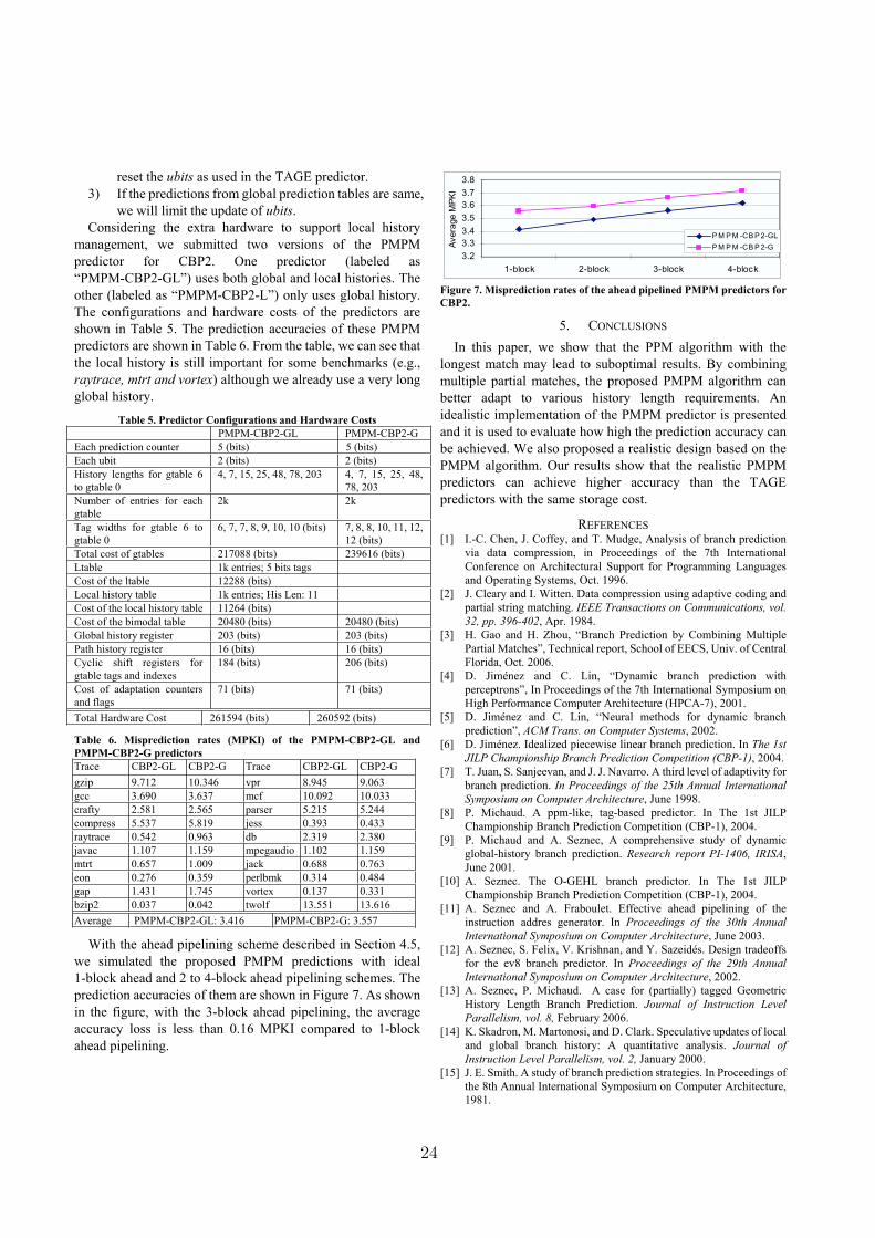
reset the ubits as used in the TAGE predictor.

3) If the predictions from global prediction tables are same,

we will limit the update of ubits.

Considering the extra hardware to support local history

management, we submitted two versions of the PMPM

predictor for CBP2. One predictor (labeled as

�PMPM-CBP2-GL�) uses both global and local histories. The

other (labeled as �PMPM-CBP2-L�) only uses global history.

The configurations and hardware costs of the predictors are

shown in Table 5. The prediction accuracies of these PMPM

predictors are shown in Table 6. From the table, we can see that

the local history is still important for some benchmarks (e.g.,

raytrace, mtrt and vortex) although we already use a very long

global history.

Table 5. Predictor Configurations and Hardware Costs

PMPM-CBP2-GL PMPM-CBP2-G

Each prediction counter 5 (bits) 5 (bits)

Each ubit 2 (bits) 2 (bits)

History lengths for gtable 6

to gtable 0

4, 7, 15, 25, 48, 78, 203 4, 7, 15, 25, 48,

78, 203

Number of entries for each

gtable

2k 2k

Tag widths for gtable 6 to

gtable 0

6, 7, 7, 8, 9, 10, 10 (bits) 7, 8, 8, 10, 11, 12,

12 (bits)

Total cost of gtables 217088 (bits) 239616 (bits)

Ltable 1k entries; 5 bits tags

Cost of the ltable 12288 (bits)

Local history table 1k entries; His Len: 11

Cost of the local history table 11264 (bits)

Cost of the bimodal table 20480 (bits) 20480 (bits)

Global history register 203 (bits) 203 (bits)

Path history register 16 (bits) 16 (bits)

Cyclic shift registers for

gtable tags and indexes

184 (bits) 206 (bits)

Cost of adaptation counters

and flags

71 (bits) 71 (bits)

Total Hardware Cost 261594 (bits) 260592 (bits)

Table 6. Misprediction rates (MPKI) of the PMPM-CBP2-GL and

PMPM-CBP2-G predictors

Trace CBP2-GL CBP2-G Trace CBP2-GL CBP2-G

gzip 9.712 10.346 vpr 8.945 9.063

gcc 3.690 3.637 mcf 10.092 10.033

crafty 2.581 2.565 parser 5.215 5.244

compress 5.537 5.819 jess 0.393 0.433

raytrace 0.542 0.963 db 2.319 2.380

javac 1.107 1.159 mpegaudio 1.102 1.159

mtrt 0.657 1.009 jack 0.688 0.763

eon 0.276 0.359 perlbmk 0.314 0.484

gap 1.431 1.745 vortex 0.137 0.331

bzip2 0.037 0.042 twolf 13.551 13.616

Average PMPM-CBP2-GL: 3.416 PMPM-CBP2-G: 3.557

With the ahead pipelining scheme described in Section 4.5,

we simulated the proposed PMPM predictions with ideal

1-block ahead and 2 to 4-block ahead pipelining schemes. The

prediction accuracies of them are shown in Figure 7. As shown

in the figure, with the 3-block ahead pipelining, the average

accuracy loss is less than 0.16 MPKI compared to 1-block

ahead pipelining.

3.2

3.3

3.4

3.5

3.6

3.7

3.8

1-block 2-block 3-block 4-block

Avera

ge M

PK

I

P M P M -CB P 2-GL

P M P M -CB P 2-G

Figure 7. Misprediction rates of the ahead pipelined PMPM predictors for

CBP2.

5. CONCLUSIONS

In this paper, we show that the PPM algorithm with the

longest match may lead to suboptimal results. By combining

multiple partial matches, the proposed PMPM algorithm can

better adapt to various history length requirements. An

idealistic implementation of the PMPM predictor is presented

and it is used to evaluate how high the prediction accuracy can

be achieved. We also proposed a realistic design based on the

PMPM algorithm. Our results show that the realistic PMPM

predictors can achieve higher accuracy than the TAGE

predictors with the same storage cost.

REFERENCES

[1] I.-C. Chen, J. Coffey, and T. Mudge, Analysis of branch prediction

via data compression, in Proceedings of the 7th International

Conference on Architectural Support for Programming Languages

and Operating Systems, Oct. 1996.

[2] J. Cleary and I. Witten. Data compression using adaptive coding and

partial string matching. IEEE Transactions on Communications, vol.

32, pp. 396-402, Apr. 1984.

[3] H. Gao and H. Zhou, �Branch Prediction by Combining Multiple

Partial Matches�, Technical report, School of EECS, Univ. of Central

Florida, Oct. 2006.

[4] D. Jiménez and C. Lin, �Dynamic branch prediction with

perceptrons�, In Proceedings of the 7th International Symposium on

High Performance Computer Architecture (HPCA-7), 2001.

[5] D. Jiménez and C. Lin, �Neural methods for dynamic branch

prediction�, ACM Trans. on Computer Systems, 2002.

[6] D. Jiménez. Idealized piecewise linear branch prediction. In The 1st

JILP Championship Branch Prediction Competition (CBP-1), 2004.

[7] T. Juan, S. Sanjeevan, and J. J. Navarro. A third level of adaptivity for

branch prediction. In Proceedings of the 25th Annual International

Symposium on Computer Architecture, June 1998.

[8] P. Michaud. A ppm-like, tag-based predictor. In The 1st JILP

Championship Branch Prediction Competition (CBP-1), 2004.

[9] P. Michaud and A. Seznec, A comprehensive study of dynamic

global-history branch prediction. Research report PI-1406, IRISA,

June 2001.

[10] A. Seznec. The O-GEHL branch predictor. In The 1st JILP

Championship Branch Prediction Competition (CBP-1), 2004.

[11] A. Seznec and A. Fraboulet. Effective ahead pipelining of the

instruction addres generator. In Proceedings of the 30th Annual

International Symposium on Computer Architecture, June 2003.

[12] A. Seznec, S. Felix, V. Krishnan, and Y. Sazeidés. Design tradeoffs

for the ev8 branch predictor. In Proceedings of the 29th Annual

International Symposium on Computer Architecture, 2002.

[13] A. Seznec, P. Michaud. A case for (partially) tagged Geometric

History Length Branch Prediction. Journal of Instruction Level

Parallelism, vol. 8, February 2006.

[14] K. Skadron, M. Martonosi, and D. Clark. Speculative updates of local

and global branch history: A quantitative analysis. Journal of

Instruction Level Parallelism, vol. 2, January 2000.

[15] J. E. Smith. A study of branch prediction strategies. In Proceedings of

the 8th Annual International Symposium on Computer Architecture,

1981.

24

Looking for limits in branch prediction with the GTL predictor

Andre Seznec

IRISA/INRIA/HIPEAC

Abstract

The geometric history length predictors, GEHL [7] and

TAGE [8], are among the most storage effective condi-

tional branch predictors. They rely on several predictor ta-

bles indexed through independent functions of the global

branch/path history and branch address. The set of used

global history lengths forms a geometric series, i.e.,

. This allows to efficiently capture correlation on

recent branch outcomes as well as on very old branches.

GEHL and TAGE differ through their final prediction

computation functions. GEHL uses a tree adder as predic-

tion computation function. TAGE uses (partial) tag match.

For realistic storage budgets (e.g., 64Kbits or 256Kbits),

TAGE was shown to be more accurate than GEHL. How-

ever, for very large storage budgets and very large num-

ber of predictor components, GEHL is more accurate than

TAGE on most benchmarks. Moreover a loop predictor can

capture part of the remaining mispredictions.

We submit the GTL predictor, combining a large GEHL

predictor, a TAGE predictor and a loop predictor, to the ide-

alistic track at CBP2.

Presentation outline

In the two past years, we have introduced the geometric

history length predictors, GEHL [7] and TAGE [8]. These

predictors are among the most storage effective branch pre-

dictors, TAGE beingmore efficient than OGEHL for limited

storage budgets. These predictors are natural candidates to

serve as basis for the design of a limit branch predictor.

In a a preliminary study, we found that, for very

large storage budget and very large number of compo-

nents, the GEHL predictor, i.e. OGEHL without dy-

namic history length fitting [7], achieves higher accuracy

than the TAGE predictor: we got respective accuracy lim-

its of 2.842 misp/KI and 3.054 misp/KI on the distributed

set of traces.

This work was partially supported by an Intel research grant, an Intelresearch equipment donation and by the European Commission in thecontext of the SARC integrated project #27648 (FP6).

Therefore the GTL predictor presented for the idealist

track at CBP-2 is an hybrid predictor, using a very large

GEHL predictor as its main component. It is combined with

a TAGE predictor and a loop predictor.

In Section 1, we first briefly present the principles of the

predictor components and the configurations used.

Section 2 presents the accuracy limits we found for the

GTL predictor and its components.

1. The GTL predictor

The GTL predictor is illustrated on Figure 1. The GTL

predictor features a GEHL predictor [7], a TAGE predictor

[8] and a loop predictor as components.

The GEHL predictor is the main predictor, since it is the

most accurate component. The GEHL predictor is used as

the base predictor component in TAGE, i.e. when there is no

partial hit on any of the TAGE components, the TAGE pre-

diction is the GEHL prediction. Moreover, the GEHL pre-

diction is used as part of the indices for the tagged compo-

nents of the TAGE predictor as well as for the components

of the metapredictor. Using a (partial) prediction as part of

the index of another table was already used on the YAGS

predictor [1] and the bimode predictor [4].

GTL uses a metapredictor to discriminate between the

TAGE and the GEHL predictions. We use a metapredictor

derived from the skewed predictor [5].

Finally, the prediction features a loop predictor. The loop

predictor provides the prediction when a loop has been suc-

cessively executed with 8 times the same number of itera-

tions as in [2].

1.1. The loop predictor

The loop predictor simply tries to identify regular loops

with constant number of iterations.

As in [2], the loop predictor provides the global predic-

tion when the loop has succesively been executed 8 times

with the same number of iterations. The loop predictor used

in the submission features 512K entries.

1.2. Common features of TAGE and GEHL

The GEHL predictor [7] and the TAGE predictor [8]

rely on several predictor tables indexed through indepen-

25

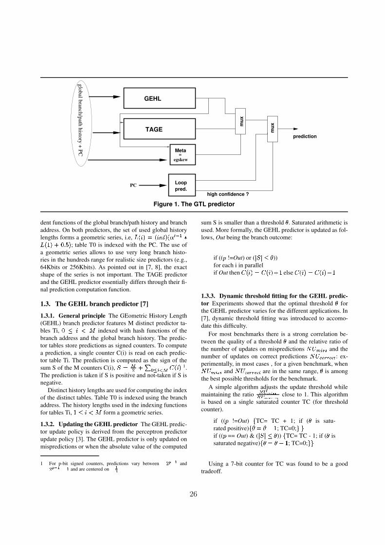
TAGE

GEHL

Loop

pred.high confidence ?

prediction

mu

x

mu

x

PC

Meta=

egskew

glo

bal b

ranch

/path

histo

ry +

PC

Figure 1. The GTL predictor

dent functions of the global branch/path history and branch

address. On both predictors, the set of used global history

lengths forms a geometric series, i.e,

; table T0 is indexed with the PC. The use of

a geometric series allows to use very long branch histo-

ries in the hundreds range for realistic size predictors (e.g.,

64Kbits or 256Kbits). As pointed out in [7, 8], the exact

shape of the series is not important. The TAGE predictor

and the GEHL predictor essentially differs through their fi-

nal prediction computation function.

1.3. The GEHL branch predictor [7]

1.3.1. General principle The GEometric History Length

(GEHL) branch predictor features M distinct predictor ta-

bles Ti, indexed with hash functions of the

branch address and the global branch history. The predic-

tor tables store predictions as signed counters. To compute

a prediction, a single counter C(i) is read on each predic-

tor table Ti. The prediction is computed as the sign of the

sum S of the M counters C(i), 1.

The prediction is taken if S is positive and not-taken if S is

negative.

Distinct history lengths are used for computing the index

of the distinct tables. Table T0 is indexed using the branch

address. The history lengths used in the indexing functions

for tables Ti, form a geometric series.

1.3.2. Updating the GEHL predictor The GEHL predic-

tor update policy is derived from the perceptron predictor

update policy [3]. The GEHL predictor is only updated on

mispredictions or when the absolute value of the computed

1 For p-bit signed counters, predictions vary between andand are centered on

sum S is smaller than a threshold . Saturated arithmetic is

used. More formally, the GEHL predictor is updated as fol-

lows, Out being the branch outcome:

if (( !=Out) or ( ))

for each i in parallel

if Out then else

1.3.3. Dynamic threshold fitting for the GEHL predic-

tor Experiments showed that the optimal threshold for

the GEHL predictor varies for the different applications. In

[7], dynamic threshold fitting was introduced to accomo-

date this difficulty.

For most benchmarks there is a strong correlation be-

tween the quality of a threshold and the relative ratio of

the number of updates on mispredictions and the

number of updates on correct predictions : ex-

perimentally, in most cases , for a given benchmark, when

and are in the same range, is among

the best possible thresholds for the benchmark.

A simple algorithm adjusts the update threshold while

maintaining the ratio close to 1. This algorithm

is based on a single saturated counter TC (for threshold

counter).

if (( !=Out) TC= TC + 1; if ( is satu-

rated positive) ; TC=0;

if (( == Out) & ( )) TC= TC - 1; if ( is

saturated negative) ; TC=0;

Using a 7-bit counter for TC was found to be a good

tradeoff.

26

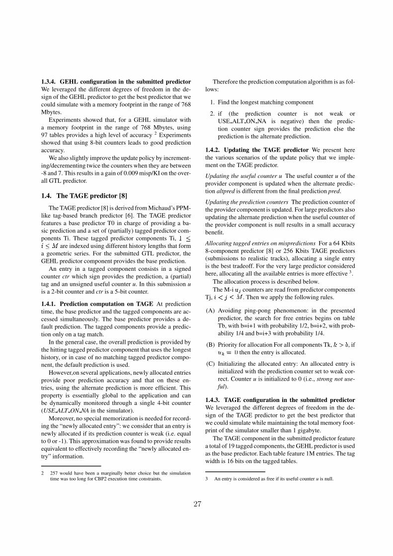
1.3.4. GEHL configuration in the submitted predictor

We leveraged the different degrees of freedom in the de-

sign of the GEHL predictor to get the best predictor that we

could simulate with a memory footprint in the range of 768

Mbytes.

Experiments showed that, for a GEHL simulator with

a memory footprint in the range of 768 Mbytes, using

97 tables provides a high level of accuracy 2 Experiments

showed that using 8-bit counters leads to good prediction

accuracy.

We also slightly improve the update policy by increment-

ing/decrementing twice the counters when they are between

-8 and 7. This results in a gain of 0.009misp/KI on the over-

all GTL predictor.

1.4. The TAGE predictor [8]

The TAGE predictor [8] is derived fromMichaud’s PPM-

like tag-based branch predictor [6]. The TAGE predictor

features a base predictor T0 in charge of providing a ba-

sic prediction and a set of (partially) tagged predictor com-

ponents Ti. These tagged predictor components Ti,

are indexed using different history lengths that form

a geometric series. For the submitted GTL predictor, the

GEHL predictor component provides the base prediction.

An entry in a tagged component consists in a signed

counter ctr which sign provides the prediction, a (partial)

tag and an unsigned useful counter u. In this submission u

is a 2-bit counter and ctr is a 5-bit counter.

1.4.1. Prediction computation on TAGE At prediction

time, the base predictor and the tagged components are ac-

cessed simultaneously. The base predictor provides a de-

fault prediction. The tagged components provide a predic-

tion only on a tag match.

In the general case, the overall prediction is provided by

the hitting tagged predictor component that uses the longest

history, or in case of no matching tagged predictor compo-

nent, the default prediction is used.

However,on several applications, newly allocated entries

provide poor prediction accuracy and that on these en-

tries, using the alternate prediction is more efficient. This

property is essentially global to the application and can

be dynamically monitored through a single 4-bit counter

(USE ALT ON NA in the simulator).

Moreover, no special memorization is needed for record-

ing the “newly allocated entry”: we consider that an entry is

newly allocated if its prediction counter is weak (i.e. equal

to 0 or -1). This approximation was found to provide results

equivalent to effectively recording the “newly allocated en-

try” information.

2 257 would have been a marginally better choice but the simulationtime was too long for CBP2 execution time constraints.

Therefore the prediction computation algorithm is as fol-

lows:

1. Find the longest matching component

2. if (the prediction counter is not weak or

USE ALT ON NA is negative) then the predic-

tion counter sign provides the prediction else the

prediction is the alternate prediction.

1.4.2. Updating the TAGE predictor We present here

the various scenarios of the update policy that we imple-

ment on the TAGE predictor.

Updating the useful counter u The useful counter u of the

provider component is updated when the alternate predic-

tion altpred is different from the final prediction pred.

Updating the prediction counters The prediction counter of

the provider component is updated. For large predictors also

updating the alternate prediction when the useful counter of

the provider component is null results in a small accuracy

benefit.

Allocating tagged entries on mispredictions For a 64 Kbits

8-component predictor [8] or 256 Kbits TAGE predictors

(submissions to realistic tracks), allocating a single entry

is the best tradeoff. For the very large predictor considered

here, allocating all the available entries is more effective 3.

The allocation process is described below.

The M-i counters are read from predictor components

Tj, . Then we apply the following rules.

(A) Avoiding ping-pong phenomenon: in the presented

predictor, the search for free entries begins on table

Tb, with b=i+1 with probability 1/2, b=i+2, with prob-

ability 1/4 and b=i+3 with probability 1/4.

(B) Priority for allocation For all components Tk, , if

then the entry is allocated.

(C) Initializing the allocated entry: An allocated entry is

initialized with the prediction counter set to weak cor-

rect. Counter u is initialized to 0 (i.e., strong not use-

ful).

1.4.3. TAGE configuration in the submitted predictor

We leveraged the different degrees of freedom in the de-

sign of the TAGE predictor to get the best predictor that

we could simulate while maintaining the total memory foot-

print of the simulator smaller than 1 gigabyte.

The TAGE component in the submitted predictor feature

a total of 19 tagged components, the GEHL predictor is used

as the base predictor. Each table feature 1M entries. The tag

width is 16 bits on the tagged tables.

3 An entry is considered as free if its useful counter u is null.

27

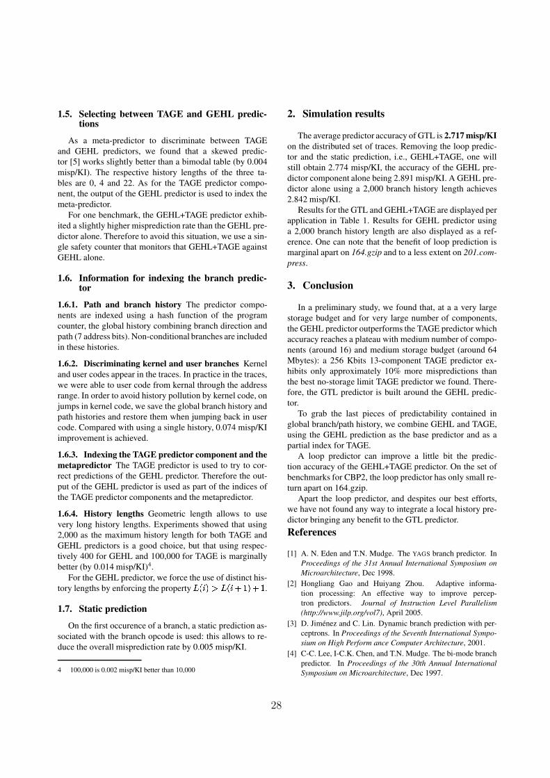
1.5. Selecting between TAGE and GEHL predic-tions

As a meta-predictor to discriminate between TAGE

and GEHL predictors, we found that a skewed predic-

tor [5] works slightly better than a bimodal table (by 0.004

misp/KI). The respective history lengths of the three ta-

bles are 0, 4 and 22. As for the TAGE predictor compo-

nent, the output of the GEHL predictor is used to index the

meta-predictor.

For one benchmark, the GEHL+TAGE predictor exhib-

ited a slightly higher misprediction rate than the GEHL pre-

dictor alone. Therefore to avoid this situation, we use a sin-

gle safety counter that monitors that GEHL+TAGE against

GEHL alone.

1.6. Information for indexing the branch predic-tor

1.6.1. Path and branch history The predictor compo-

nents are indexed using a hash function of the program

counter, the global history combining branch direction and

path (7 address bits). Non-conditional branches are included

in these histories.

1.6.2. Discriminating kernel and user branches Kernel

and user codes appear in the traces. In practice in the traces,

we were able to user code from kernal through the address

range. In order to avoid history pollution by kernel code, on

jumps in kernel code, we save the global branch history and

path histories and restore them when jumping back in user

code. Compared with using a single history, 0.074 misp/KI

improvement is achieved.

1.6.3. Indexing the TAGE predictor component and the

metapredictor The TAGE predictor is used to try to cor-

rect predictions of the GEHL predictor. Therefore the out-

put of the GEHL predictor is used as part of the indices of

the TAGE predictor components and the metapredictor.

1.6.4. History lengths Geometric length allows to use

very long history lengths. Experiments showed that using

2,000 as the maximum history length for both TAGE and

GEHL predictors is a good choice, but that using respec-

tively 400 for GEHL and 100,000 for TAGE is marginally

better (by 0.014 misp/KI)4.

For the GEHL predictor, we force the use of distinct his-

tory lengths by enforcing the property .

1.7. Static prediction

On the first occurence of a branch, a static prediction as-

sociated with the branch opcode is used: this allows to re-

duce the overall misprediction rate by 0.005 misp/KI.

4 100,000 is 0.002 misp/KI better than 10,000

2. Simulation results

The average predictor accuracy of GTL is 2.717misp/KI

on the distributed set of traces. Removing the loop predic-

tor and the static prediction, i.e., GEHL+TAGE, one will

still obtain 2.774 misp/KI, the accuracy of the GEHL pre-

dictor component alone being 2.891 misp/KI. A GEHL pre-

dictor alone using a 2,000 branch history length achieves

2.842 misp/KI.

Results for the GTL and GEHL+TAGE are displayed per

application in Table 1. Results for GEHL predictor using

a 2,000 branch history length are also displayed as a ref-

erence. One can note that the benefit of loop prediction is

marginal apart on 164.gzip and to a less extent on 201.com-

press.

3. Conclusion

In a preliminary study, we found that, at a a very large

storage budget and for very large number of components,

the GEHL predictor outperforms the TAGE predictor which

accuracy reaches a plateau with medium number of compo-

nents (around 16) and medium storage budget (around 64

Mbytes): a 256 Kbits 13-component TAGE predictor ex-

hibits only approximately 10% more mispredictions than

the best no-storage limit TAGE predictor we found. There-

fore, the GTL predictor is built around the GEHL predic-

tor.

To grab the last pieces of predictability contained in

global branch/path history, we combine GEHL and TAGE,

using the GEHL prediction as the base predictor and as a

partial index for TAGE.

A loop predictor can improve a little bit the predic-

tion accuracy of the GEHL+TAGE predictor. On the set of

benchmarks for CBP2, the loop predictor has only small re-

turn apart on 164.gzip.

Apart the loop predictor, and despites our best efforts,

we have not found any way to integrate a local history pre-

dictor bringing any benefit to the GTL predictor.

References

[1] A. N. Eden and T.N. Mudge. The YAGS branch predictor. In

Proceedings of the 31st Annual International Symposium on

Microarchitecture, Dec 1998.

[2] Hongliang Gao and Huiyang Zhou. Adaptive informa-

tion processing: An effective way to improve percep-

tron predictors. Journal of Instruction Level Parallelism

(http://www.jilp.org/vol7), April 2005.

[3] D. Jimenez and C. Lin. Dynamic branch prediction with per-

ceptrons. In Proceedings of the Seventh International Sympo-

sium on High Perform ance Computer Architecture, 2001.

[4] C-C. Lee, I-C.K. Chen, and T.N. Mudge. The bi-mode branch

predictor. In Proceedings of the 30th Annual International

Symposium on Microarchitecture, Dec 1997.

28

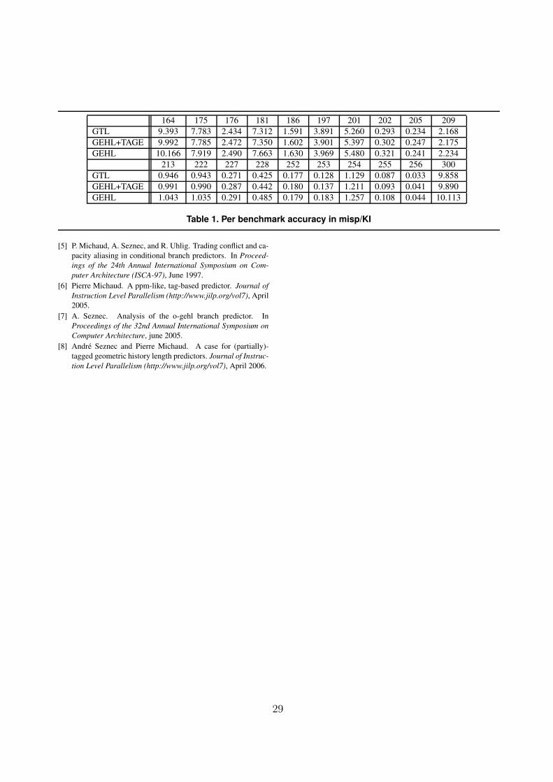
164 175 176 181 186 197 201 202 205 209

GTL 9.393 7.783 2.434 7.312 1.591 3.891 5.260 0.293 0.234 2.168

GEHL+TAGE 9.992 7.785 2.472 7.350 1.602 3.901 5.397 0.302 0.247 2.175

GEHL 10.166 7.919 2.490 7.663 1.630 3.969 5.480 0.321 0.241 2.234

213 222 227 228 252 253 254 255 256 300

GTL 0.946 0.943 0.271 0.425 0.177 0.128 1.129 0.087 0.033 9.858

GEHL+TAGE 0.991 0.990 0.287 0.442 0.180 0.137 1.211 0.093 0.041 9.890

GEHL 1.043 1.035 0.291 0.485 0.179 0.183 1.257 0.108 0.044 10.113

Table 1. Per benchmark accuracy in misp/KI

[5] P. Michaud, A. Seznec, and R. Uhlig. Trading conflict and ca-

pacity aliasing in conditional branch predictors. In Proceed-

ings of the 24th Annual International Symposium on Com-

puter Architecture (ISCA-97), June 1997.

[6] Pierre Michaud. A ppm-like, tag-based predictor. Journal of

Instruction Level Parallelism (http://www.jilp.org/vol7), April

2005.

[7] A. Seznec. Analysis of the o-gehl branch predictor. In

Proceedings of the 32nd Annual International Symposium on

Computer Architecture, june 2005.

[8] Andre Seznec and Pierre Michaud. A case for (partially)-

tagged geometric history length predictors. Journal of Instruc-

tion Level Parallelism (http://www.jilp.org/vol7), April 2006.

29

Neuro-PPM Branch Prediction

Ram Srinivasan† *, Eitan Frachtenberg†, Olaf Lubeck†, Scott Pakin†, Jeanine Cook*

†CCS-3 Modeling, Algorithms and Informatics. Los Alamos National Laboratory.*Klipsch School of Electrical and Computer Engineering. New Mexico State University.

{[email protected], [email protected], [email protected], [email protected], [email protected]}

Abstract

Historically, Markovian predictors have been very success-

ful in predicting branch outcomes. In this work we propose a

hybrid scheme that employs two Prediction by Partial Match-

ing (PPM) Markovian predictors, one that predicts based on

local branch histories and one based on global branch his-

tories. The two independent predictions are combined us-

ing a neural network. On the CBP-2 traces the proposed

scheme achieves over twice the prediction accuracy of the

gshare predictor.

1. Introduction

Data compression and branch prediction share many sim-

ilarities. Given a stream of symbols (e.g., ASCII characters

for text compression or past branch outcomes for branch pre-

diction), the goal in both cases is to predict future symbols

as accurately as possible. One common way of achieving

this goal in data compression is Prediction by Partial Match-

ing (PPM) [1, 5]. PPM is a Markov predictor in which the

prediction is a function of the current state. The state infor-

mation in an mth-order PPM predictor is an ensemble of the

m most recent symbols. If the pattern formed by the m re-

cent symbols has occurred earlier, the symbol following the

pattern is used as the prediction.

As an example of how PPM works, consider the sample

stream of binary symbols presented in Figure 1. To predict

what symbol will appear at position 0 we look for clues ear-

lier in the stream. For example, we observe that the pre-

vious symbol is a 1. The last time a 1 was observed—at

position 2—the following symbol was a 1. Hence, we can

predict that position 0 will be a 1. However, we do not

have to limit ourselves to examining a single-symbol pattern.

The last time 1 1 (positions 2 and 1) appeared was at posi-

tions 10 and 9 and the subsequent symbol (position 8) was a

0 so we can predict 0. We find the next longer pattern, 0 1 1

(at positions {3, 2, 1}), at positions {13, 12, 11} with posi-

tion 10 predicting 1. The longest pattern with a prior match

is 0 1 0 1 0 0 1 1 (positions {8, 7, 6, 5, 4, 3, 2, 1}) at positions

{24, 23, 22, 21, 20, 19, 18, 17}. The subsequent symbol is 0

so we can choose 0 as our best guess for position 0’s value.

Generally, predictors that use longer patterns to make a

prediction are more accurate than those that use shorter pat-

terns. However, with longer patterns, the likelihood of the

same pattern having occurred earlier diminishes and hence

the ability to predict decreases. To address this problem, an

mth-order PPM scheme first attempts to predict using the m

most recent symbols. Progressively smaller patterns are uti-

lized until a matching pattern is found and a prediction can

thereby be made.

In the context of branch prediction, the symbols are

branch outcomes. The past outcomes used in prediction can

be either local or global. In a local scheme, the prediction

for a given branch is based solely on the past outcomes of

the (static) branch that we are trying to predict. In contrast,

a global scheme uses outcomes from all branches to make

the prediction. In this paper we propose a hybrid PPM-based

branch predictor that employs pattern matching on both lo-

cal and global histories. The predictions based on the two

histories are combined using a perceptron-based neural net-

work [3] to achieve a high prediction accuracy. Hardware

implementability is not our goal. Rather, we determine the

best prediction accuracy that can be achieved from PPM-like

schemes given virtually unlimited memory and processing

time. This approach corresponds to the “idealistic” track

of the 2nd JILP Championship Branch Prediction Compe-

tition [2].

There are many optimizations and heuristics that improve

the speed, accuracy, and memory utilization of the basic PPM

method. In Section 2 we present our implementation tech-

nique and a set of modifications that prove empirically to

be beneficial to performance or resource usage. Finally, we

draw some conclusions in Section 3.

2. Implementation

Figure 2 shows the high-level block diagram of the Neuro-

PPM predictor. Our scheme consists of two PPM-based pre-

dictors [1], one that uses local-history information and the

other that uses global-history information to identify patterns

and predict branch outcomes. For a given branch, both PPM

predictors are invoked to predict the branch outcome. The

two predictions are combined using a perceptron-based neu-

30

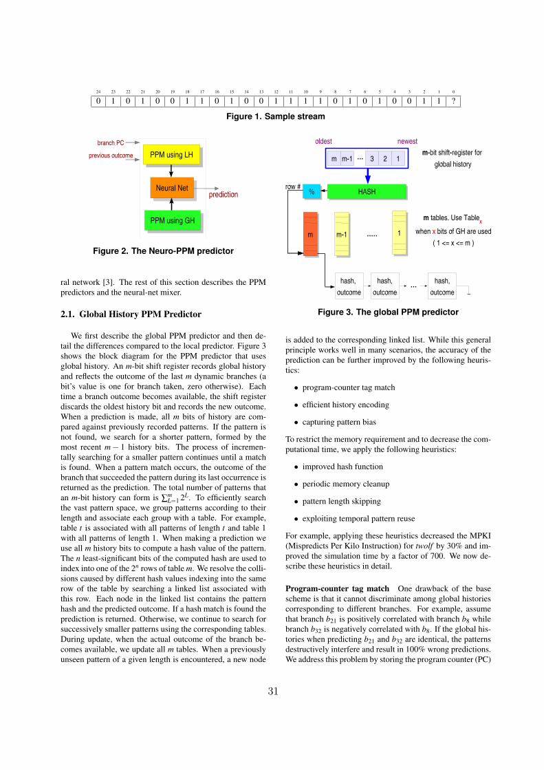
24 23 22 21 20 19 18 17 16 15 14 13 12 11 10 9 8 7 6 5 4 3 2 1 0

0 1 0 1 0 0 1 1 0 1 0 0 1 1 1 1 0 1 0 1 0 0 1 1 ?

Figure 1. Sample stream

Figure 2. The Neuro-PPM predictor

ral network [3]. The rest of this section describes the PPM

predictors and the neural-net mixer.

2.1. Global History PPM Predictor

We first describe the global PPM predictor and then de-

tail the differences compared to the local predictor. Figure 3

shows the block diagram for the PPM predictor that uses

global history. An m-bit shift register records global history

and reflects the outcome of the last m dynamic branches (a

bit’s value is one for branch taken, zero otherwise). Each

time a branch outcome becomes available, the shift register

discards the oldest history bit and records the new outcome.

When a prediction is made, all m bits of history are com-

pared against previously recorded patterns. If the pattern is

not found, we search for a shorter pattern, formed by the

most recent m − 1 history bits. The process of incremen-

tally searching for a smaller pattern continues until a match

is found. When a pattern match occurs, the outcome of the

branch that succeeded the pattern during its last occurrence is

returned as the prediction. The total number of patterns that

an m-bit history can form is ∑mL=1 2L. To efficiently search

the vast pattern space, we group patterns according to their

length and associate each group with a table. For example,

table t is associated with all patterns of length t and table 1

with all patterns of length 1. When making a prediction we

use all m history bits to compute a hash value of the pattern.

The n least-significant bits of the computed hash are used to

index into one of the 2n rows of table m. We resolve the colli-

sions caused by different hash values indexing into the same

row of the table by searching a linked list associated with

this row. Each node in the linked list contains the pattern

hash and the predicted outcome. If a hash match is found the

prediction is returned. Otherwise, we continue to search for

successively smaller patterns using the corresponding tables.

During update, when the actual outcome of the branch be-

comes available, we update all m tables. When a previously

unseen pattern of a given length is encountered, a new node

Figure 3. The global PPM predictor

is added to the corresponding linked list. While this general

principle works well in many scenarios, the accuracy of the

prediction can be further improved by the following heuris-

tics:

• program-counter tag match

• efficient history encoding

• capturing pattern bias

To restrict the memory requirement and to decrease the com-

putational time, we apply the following heuristics:

• improved hash function

• periodic memory cleanup

• pattern length skipping

• exploiting temporal pattern reuse

For example, applying these heuristics decreased the MPKI

(Mispredicts Per Kilo Instruction) for twolf by 30% and im-

proved the simulation time by a factor of 700. We now de-

scribe these heuristics in detail.

Program-counter tag match One drawback of the base

scheme is that it cannot discriminate among global histories

corresponding to different branches. For example, assume

that branch b21 is positively correlated with branch b8 while

branch b32 is negatively correlated with b8. If the global his-

tories when predicting b21 and b32 are identical, the patterns

destructively interfere and result in 100% wrong predictions.

We address this problem by storing the program counter (PC)

31

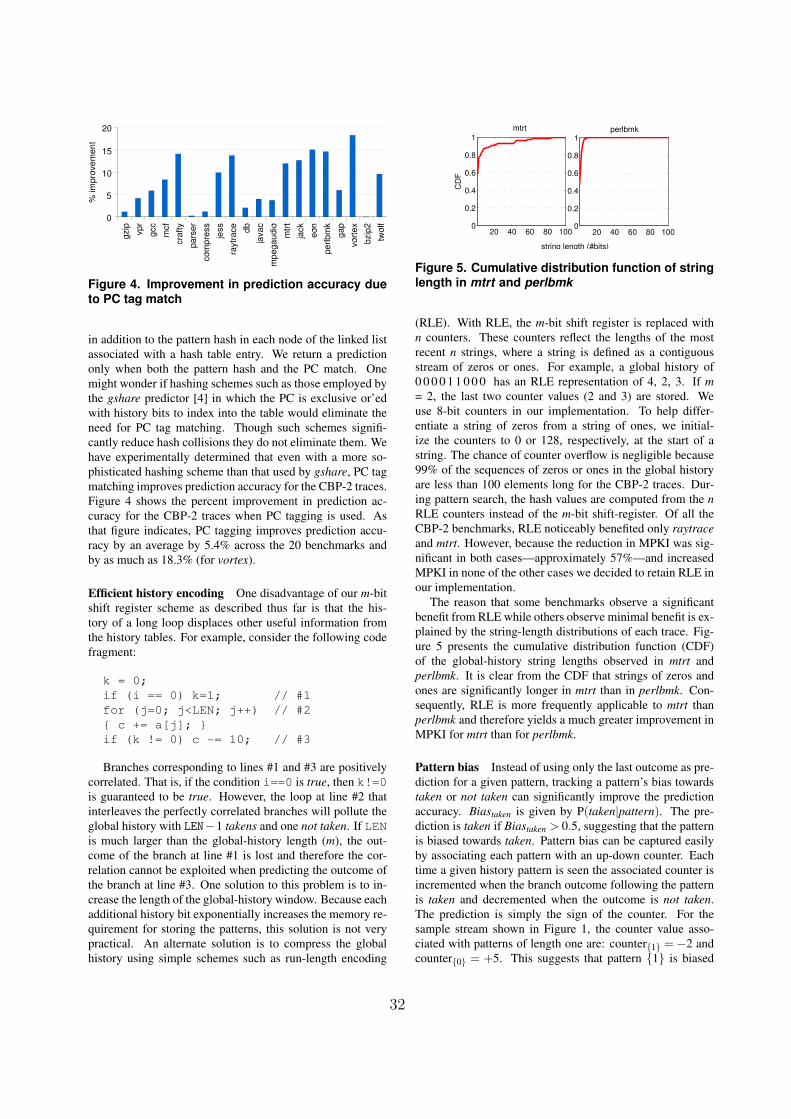
Figure 4. Improvement in prediction accuracy dueto PC tag match

in addition to the pattern hash in each node of the linked list

associated with a hash table entry. We return a prediction

only when both the pattern hash and the PC match. One

might wonder if hashing schemes such as those employed by

the gshare predictor [4] in which the PC is exclusive or’ed

with history bits to index into the table would eliminate the

need for PC tag matching. Though such schemes signifi-

cantly reduce hash collisions they do not eliminate them. We

have experimentally determined that even with a more so-

phisticated hashing scheme than that used by gshare, PC tag

matching improves prediction accuracy for the CBP-2 traces.

Figure 4 shows the percent improvement in prediction ac-

curacy for the CBP-2 traces when PC tagging is used. As

that figure indicates, PC tagging improves prediction accu-

racy by an average by 5.4% across the 20 benchmarks and

by as much as 18.3% (for vortex).

Efficient history encoding One disadvantage of our m-bit

shift register scheme as described thus far is that the his-

tory of a long loop displaces other useful information from

the history tables. For example, consider the following code

fragment:

k = 0;

if (i == 0) k=1; // #1

for (j=0; j<LEN; j++) // #2

{ c += a[j]; }

if (k != 0) c -= 10; // #3

Branches corresponding to lines #1 and #3 are positively

correlated. That is, if the condition i==0 is true, then k!=0

is guaranteed to be true. However, the loop at line #2 that

interleaves the perfectly correlated branches will pollute the

global history with LEN−1 takens and one not taken. If LEN

is much larger than the global-history length (m), the out-

come of the branch at line #1 is lost and therefore the cor-

relation cannot be exploited when predicting the outcome of

the branch at line #3. One solution to this problem is to in-

crease the length of the global-history window. Because each

additional history bit exponentially increases the memory re-

quirement for storing the patterns, this solution is not very

practical. An alternate solution is to compress the global

history using simple schemes such as run-length encoding

20 40 60 80 1000

0.2

0.4

0.6

0.8

1mtrt

CD

F

20 40 60 80 1000

0.2

0.4

0.6

0.8

1perlbmk

string length (#bits)

Figure 5. Cumulative distribution function of stringlength in mtrt and perlbmk

(RLE). With RLE, the m-bit shift register is replaced with

n counters. These counters reflect the lengths of the most

recent n strings, where a string is defined as a contiguous

stream of zeros or ones. For example, a global history of

0 0 0 0 1 1 0 0 0 has an RLE representation of 4, 2, 3. If m

= 2, the last two counter values (2 and 3) are stored. We

use 8-bit counters in our implementation. To help differ-

entiate a string of zeros from a string of ones, we initial-

ize the counters to 0 or 128, respectively, at the start of a

string. The chance of counter overflow is negligible because

99% of the sequences of zeros or ones in the global history

are less than 100 elements long for the CBP-2 traces. Dur-

ing pattern search, the hash values are computed from the n

RLE counters instead of the m-bit shift-register. Of all the

CBP-2 benchmarks, RLE noticeably benefited only raytrace

and mtrt. However, because the reduction in MPKI was sig-

nificant in both cases—approximately 57%—and increased

MPKI in none of the other cases we decided to retain RLE in

our implementation.

The reason that some benchmarks observe a significant

benefit from RLE while others observe minimal benefit is ex-

plained by the string-length distributions of each trace. Fig-

ure 5 presents the cumulative distribution function (CDF)

of the global-history string lengths observed in mtrt and

perlbmk. It is clear from the CDF that strings of zeros and

ones are significantly longer in mtrt than in perlbmk. Con-

sequently, RLE is more frequently applicable to mtrt than

perlbmk and therefore yields a much greater improvement in

MPKI for mtrt than for perlbmk.

Pattern bias Instead of using only the last outcome as pre-

diction for a given pattern, tracking a pattern’s bias towards

taken or not taken can significantly improve the prediction

accuracy. Biastaken is given by P(taken|pattern). The pre-

diction is taken if Biastaken > 0.5, suggesting that the pattern

is biased towards taken. Pattern bias can be captured easily

by associating each pattern with an up-down counter. Each

time a given history pattern is seen the associated counter is

incremented when the branch outcome following the pattern

is taken and decremented when the outcome is not taken.

The prediction is simply the sign of the counter. For the

sample stream shown in Figure 1, the counter value asso-

ciated with patterns of length one are: counter{1} = −2 and

counter{0} = +5. This suggests that pattern {1} is biased

32

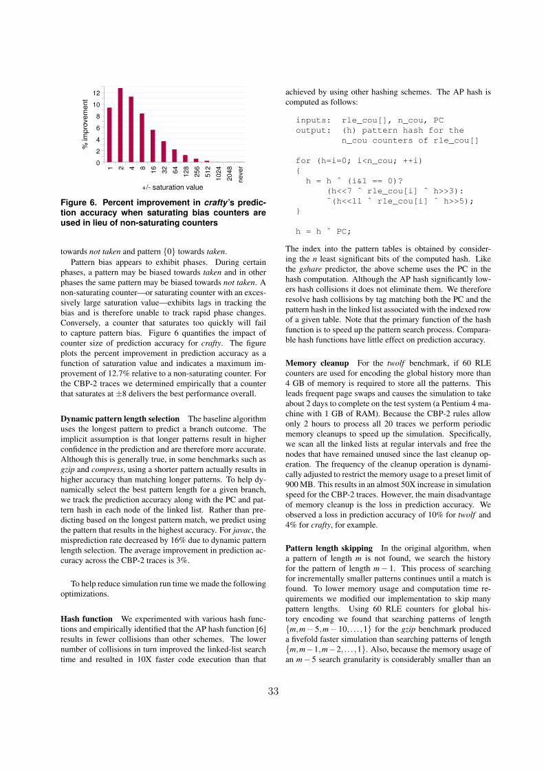
Figure 6. Percent improvement in crafty ’s predic-tion accuracy when saturating bias counters areused in lieu of non-saturating counters

towards not taken and pattern {0} towards taken.

Pattern bias appears to exhibit phases. During certain

phases, a pattern may be biased towards taken and in other

phases the same pattern may be biased towards not taken. A

non-saturating counter—or saturating counter with an exces-

sively large saturation value—exhibits lags in tracking the

bias and is therefore unable to track rapid phase changes.

Conversely, a counter that saturates too quickly will fail

to capture pattern bias. Figure 6 quantifies the impact of

counter size of prediction accuracy for crafty. The figure

plots the percent improvement in prediction accuracy as a

function of saturation value and indicates a maximum im-

provement of 12.7% relative to a non-saturating counter. For

the CBP-2 traces we determined empirically that a counter

that saturates at ±8 delivers the best performance overall.

Dynamic pattern length selection The baseline algorithm

uses the longest pattern to predict a branch outcome. The

implicit assumption is that longer patterns result in higher

confidence in the prediction and are therefore more accurate.

Although this is generally true, in some benchmarks such as

gzip and compress, using a shorter pattern actually results in

higher accuracy than matching longer patterns. To help dy-

namically select the best pattern length for a given branch,

we track the prediction accuracy along with the PC and pat-

tern hash in each node of the linked list. Rather than pre-

dicting based on the longest pattern match, we predict using

the pattern that results in the highest accuracy. For javac, the

misprediction rate decreased by 16% due to dynamic pattern

length selection. The average improvement in prediction ac-

curacy across the CBP-2 traces is 3%.

To help reduce simulation run time we made the following

optimizations.

Hash function We experimented with various hash func-

tions and empirically identified that the AP hash function [6]

results in fewer collisions than other schemes. The lower

number of collisions in turn improved the linked-list search

time and resulted in 10X faster code execution than that

achieved by using other hashing schemes. The AP hash is

computed as follows:

inputs: rle_cou[], n_cou, PC

output: (h) pattern hash for the

n_cou counters of rle_cou[]

for (h=i=0; i<n_cou; ++i)

{

h = h ˆ (i&1 == 0)?

(h<<7 ˆ rle_cou[i] ˆ h>>3):

˜(h<<11 ˆ rle_cou[i] ˆ h>>5);

}

h = h ˆ PC;

The index into the pattern tables is obtained by consider-

ing the n least significant bits of the computed hash. Like

the gshare predictor, the above scheme uses the PC in the

hash computation. Although the AP hash significantly low-

ers hash collisions it does not eliminate them. We therefore

resolve hash collisions by tag matching both the PC and the

pattern hash in the linked list associated with the indexed row

of a given table. Note that the primary function of the hash

function is to speed up the pattern search process. Compara-

ble hash functions have little effect on prediction accuracy.

Memory cleanup For the twolf benchmark, if 60 RLE

counters are used for encoding the global history more than

4 GB of memory is required to store all the patterns. This

leads frequent page swaps and causes the simulation to take

about 2 days to complete on the test system (a Pentium 4 ma-

chine with 1 GB of RAM). Because the CBP-2 rules allow

only 2 hours to process all 20 traces we perform periodic

memory cleanups to speed up the simulation. Specifically,

we scan all the linked lists at regular intervals and free the

nodes that have remained unused since the last cleanup op-

eration. The frequency of the cleanup operation is dynami-

cally adjusted to restrict the memory usage to a preset limit of

900 MB. This results in an almost 50X increase in simulation

speed for the CBP-2 traces. However, the main disadvantage

of memory cleanup is the loss in prediction accuracy. We

observed a loss in prediction accuracy of 10% for twolf and

4% for crafty, for example.

Pattern length skipping In the original algorithm, when

a pattern of length m is not found, we search the history

for the pattern of length m− 1. This process of searching

for incrementally smaller patterns continues until a match is

found. To lower memory usage and computation time re-

quirements we modified our implementation to skip many

pattern lengths. Using 60 RLE counters for global his-

tory encoding we found that searching patterns of length

{m,m− 5,m− 10, . . . ,1} for the gzip benchmark produced

a fivefold faster simulation than searching patterns of length

{m,m−1,m−2, . . . ,1}. Also, because the memory usage of

an m− 5 search granularity is considerably smaller than an

33

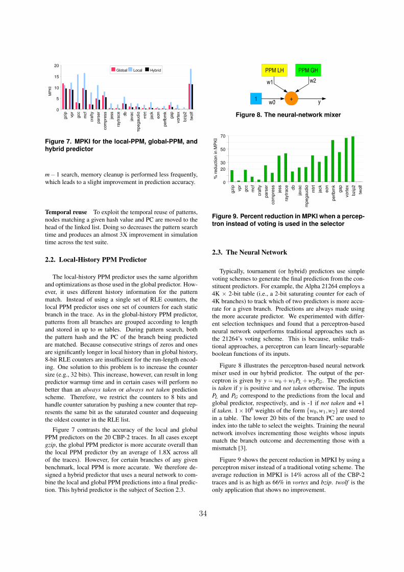
Figure 7. MPKI for the local-PPM, global-PPM, andhybrid predictor

m−1 search, memory cleanup is performed less frequently,

which leads to a slight improvement in prediction accuracy.

Temporal reuse To exploit the temporal reuse of patterns,

nodes matching a given hash value and PC are moved to the

head of the linked list. Doing so decreases the pattern search

time and produces an almost 3X improvement in simulation

time across the test suite.

2.2. Local-History PPM Predictor

The local-history PPM predictor uses the same algorithm

and optimizations as those used in the global predictor. How-

ever, it uses different history information for the pattern

match. Instead of using a single set of RLE counters, the

local PPM predictor uses one set of counters for each static

branch in the trace. As in the global-history PPM predictor,

patterns from all branches are grouped according to length

and stored in up to m tables. During pattern search, both

the pattern hash and the PC of the branch being predicted

are matched. Because consecutive strings of zeros and ones

are significantly longer in local history than in global history,

8-bit RLE counters are insufficient for the run-length encod-

ing. One solution to this problem is to increase the counter

size (e.g., 32 bits). This increase, however, can result in long

predictor warmup time and in certain cases will perform no

better than an always taken or always not taken prediction

scheme. Therefore, we restrict the counters to 8 bits and

handle counter saturation by pushing a new counter that rep-

resents the same bit as the saturated counter and dequeuing

the oldest counter in the RLE list.

Figure 7 contrasts the accuracy of the local and global

PPM predictors on the 20 CBP-2 traces. In all cases except

gzip, the global PPM predictor is more accurate overall than

the local PPM predictor (by an average of 1.8X across all

of the traces). However, for certain branches of any given

benchmark, local PPM is more accurate. We therefore de-

signed a hybrid predictor that uses a neural network to com-

bine the local and global PPM predictions into a final predic-

tion. This hybrid predictor is the subject of Section 2.3.

Figure 8. The neural-network mixer

Figure 9. Percent reduction in MPKI when a percep-tron instead of voting is used in the selector

2.3. The Neural Network

Typically, tournament (or hybrid) predictors use simple

voting schemes to generate the final prediction from the con-

stituent predictors. For example, the Alpha 21264 employs a

4K × 2-bit table (i.e., a 2-bit saturating counter for each of

4K branches) to track which of two predictors is more accu-

rate for a given branch. Predictions are always made using

the more accurate predictor. We experimented with differ-

ent selection techniques and found that a perceptron-based

neural network outperforms traditional approaches such as

the 21264’s voting scheme. This is because, unlike tradi-

tional approaches, a perceptron can learn linearly-separable

boolean functions of its inputs.

Figure 8 illustrates the perceptron-based neural network

mixer used in our hybrid predictor. The output of the per-

ceptron is given by y = w0 + w1PL + w2PG. The prediction

is taken if y is positive and not taken otherwise. The inputs

PL and PG correspond to the predictions from the local and

global predictor, respectively, and is -1 if not taken and +1

if taken. 1×106 weights of the form {w0,w1,w2} are stored

in a table. The lower 20 bits of the branch PC are used to

index into the table to select the weights. Training the neural

network involves incrementing those weights whose inputs

match the branch outcome and decrementing those with a

mismatch [3].

Figure 9 shows the percent reduction in MPKI by using a

perceptron mixer instead of a traditional voting scheme. The

average reduction in MPKI is 14% across all of the CBP-2

traces and is as high as 66% in vortex and bzip. twolf is the

only application that shows no improvement.

34

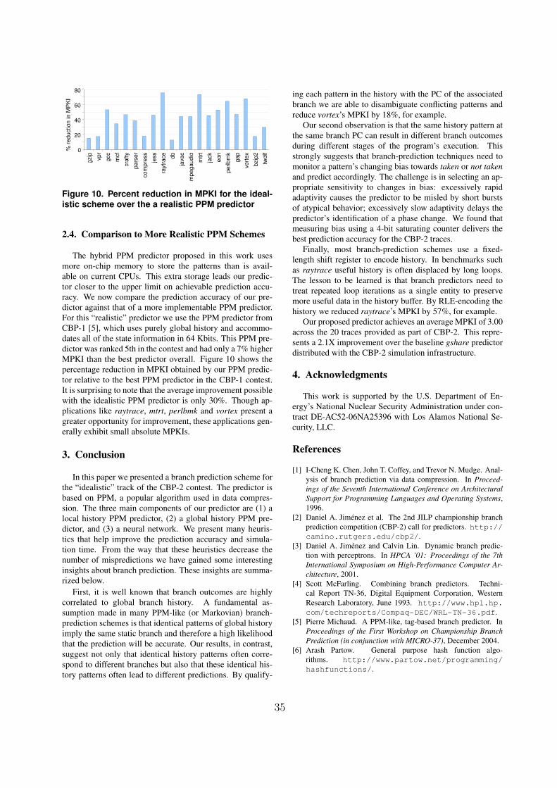
Figure 10. Percent reduction in MPKI for the ideal-istic scheme over the a realistic PPM predictor

2.4. Comparison to More Realistic PPM Schemes

The hybrid PPM predictor proposed in this work uses

more on-chip memory to store the patterns than is avail-

able on current CPUs. This extra storage leads our predic-

tor closer to the upper limit on achievable prediction accu-

racy. We now compare the prediction accuracy of our pre-

dictor against that of a more implementable PPM predictor.

For this “realistic” predictor we use the PPM predictor from

CBP-1 [5], which uses purely global history and accommo-

dates all of the state information in 64 Kbits. This PPM pre-

dictor was ranked 5th in the contest and had only a 7% higher

MPKI than the best predictor overall. Figure 10 shows the

percentage reduction in MPKI obtained by our PPM predic-

tor relative to the best PPM predictor in the CBP-1 contest.

It is surprising to note that the average improvement possible

with the idealistic PPM predictor is only 30%. Though ap-

plications like raytrace, mtrt, perlbmk and vortex present a

greater opportunity for improvement, these applications gen-

erally exhibit small absolute MPKIs.

3. Conclusion

In this paper we presented a branch prediction scheme for

the “idealistic” track of the CBP-2 contest. The predictor is

based on PPM, a popular algorithm used in data compres-

sion. The three main components of our predictor are (1) a

local history PPM predictor, (2) a global history PPM pre-

dictor, and (3) a neural network. We present many heuris-

tics that help improve the prediction accuracy and simula-

tion time. From the way that these heuristics decrease the

number of mispredictions we have gained some interesting

insights about branch prediction. These insights are summa-

rized below.

First, it is well known that branch outcomes are highly

correlated to global branch history. A fundamental as-

sumption made in many PPM-like (or Markovian) branch-

prediction schemes is that identical patterns of global history

imply the same static branch and therefore a high likelihood

that the prediction will be accurate. Our results, in contrast,

suggest not only that identical history patterns often corre-

spond to different branches but also that these identical his-

tory patterns often lead to different predictions. By qualify-

ing each pattern in the history with the PC of the associated

branch we are able to disambiguate conflicting patterns and

reduce vortex’s MPKI by 18%, for example.

Our second observation is that the same history pattern at

the same branch PC can result in different branch outcomes

during different stages of the program’s execution. This

strongly suggests that branch-prediction techniques need to

monitor a pattern’s changing bias towards taken or not taken

and predict accordingly. The challenge is in selecting an ap-

propriate sensitivity to changes in bias: excessively rapid

adaptivity causes the predictor to be misled by short bursts

of atypical behavior; excessively slow adaptivity delays the

predictor’s identification of a phase change. We found that

measuring bias using a 4-bit saturating counter delivers the

best prediction accuracy for the CBP-2 traces.

Finally, most branch-prediction schemes use a fixed-

length shift register to encode history. In benchmarks such

as raytrace useful history is often displaced by long loops.

The lesson to be learned is that branch predictors need to

treat repeated loop iterations as a single entity to preserve

more useful data in the history buffer. By RLE-encoding the

history we reduced raytrace’s MPKI by 57%, for example.

Our proposed predictor achieves an average MPKI of 3.00

across the 20 traces provided as part of CBP-2. This repre-

sents a 2.1X improvement over the baseline gshare predictor

distributed with the CBP-2 simulation infrastructure.

4. Acknowledgments

This work is supported by the U.S. Department of En-

ergy’s National Nuclear Security Administration under con-

tract DE-AC52-06NA25396 with Los Alamos National Se-

curity, LLC.

References

[1] I-Cheng K. Chen, John T. Coffey, and Trevor N. Mudge. Anal-

ysis of branch prediction via data compression. In Proceed-

ings of the Seventh International Conference on Architectural

Support for Programming Languages and Operating Systems,

1996.

[2] Daniel A. Jimenez et al. The 2nd JILP championship branch

prediction competition (CBP-2) call for predictors. http://

camino.rutgers.edu/cbp2/.

[3] Daniel A. Jimenez and Calvin Lin. Dynamic branch predic-

tion with perceptrons. In HPCA ’01: Proceedings of the 7th

International Symposium on High-Performance Computer Ar-

chitecture, 2001.

[4] Scott McFarling. Combining branch predictors. Techni-

cal Report TN-36, Digital Equipment Corporation, Western

Research Laboratory, June 1993. http://www.hpl.hp.

com/techreports/Compaq-DEC/WRL-TN-36.pdf.

[5] Pierre Michaud. A PPM-like, tag-based branch predictor. In

Proceedings of the First Workshop on Championship Branch

Prediction (in conjunction with MICRO-37), December 2004.

[6] Arash Partow. General purpose hash function algo-

rithms. http://www.partow.net/programming/

hashfunctions/.

35

Documents

The Second Journal of Instruction-Level Parallelism