The second Chinese glacier inventory: data, methods and ... · The second Chinese glacier inventory: data, methods and results ... The second Chinese glacier inventory was compiled

The second Chinese glacier inventory: data, methods and results

Wanqin GUO,1 Shiyin LIU,1 Junli XU,1 Lizong WU,2 Donghui SHANGGUAN,1

Xiaojun YAO,3 Junfeng WEI,1 Weijia BAO,1 Pengchun YU,4 Qiao LIU,5 Zongli JIANG6

1State Key Laboratory of Cryospheric Sciences, Cold and Arid Regions Environmental and Engineering Research Institute,Chinese Academy of Sciences, Lanzhou, China

2Laboratory of Remote Sensing and Geospatial Science, Cold and Arid Regions Environmental and Engineering ResearchInstitute, Chinese Academy of Sciences, Lanzhou, China

3Geography and Environment College, Northwest Normal University, Lanzhou, China4Fujian Institute of Geology Survey and Research, Fuzhou, China

5Institute of Mountain Hazards and Environment, Chinese Academy of Sciences, Chengdu, China6Hunan Province Key Laboratory of Coal Resources Clean-Utilization and Mine Environment Protection, Hunan University of

Science and Technology, Xiangtan, ChinaCorrespondence: Wanqin Guo <[email protected]>

ABSTRACT. The second Chinese glacier inventory was compiled based on 218 Landsat TM/ETM+scenes acquired mainly during 2006–10. The widely used band ratio segmentation method was appliedas the first step in delineating glacier outlines, and then intensive manual improvements wereperformed. The Shuttle Radar Topography Mission digital elevation model was used to derive altitudinalattributes of glaciers. The boundaries of some glaciers measured by real-time kinematic differential GPSor digitized from high-resolution images were used as references to validate the accuracy of themethods used to delineate glaciers, which resulted in positioning errors of ��10m for manuallyimproved clean-ice outlines and �30m for manually digitized outlines of debris-covered parts. Theglacier area error of the compiled inventory, evaluated using these two positioning accuracies, was�3.2%. The compiled parts of the new inventory have a total area of 43 087 km2, in which 1723glaciers were covered by debris, with a total debris-covered area of 1494 km2. The area of uncompiledglaciers from the digitized first Chinese glacier inventory is �8753 km2, mainly distributed in thesoutheastern Tibetan Plateau, where no images of acceptable quality for glacier outline delineation canbe found during 2006–10.

KEYWORDS: debris-covered glaciers, glacier delineation, glacier mapping, mountain glaciers, remotesensing

1. INTRODUCTIONThe sensitivity of glaciers to local climate change makesthem an obvious and widely used indicator of global climatechange (Vaughan and others, 2013). Global warming duringrecent decades has had significant impacts on the world’sglaciers, which have experienced intensified ice mass lossinduced by strengthened ablation, and thus thinning (e.g.Rivera and others, 2007; James and others, 2012; Lee andothers, 2013; Racoviteanu and others, 2014), along withuniversal retreat and shrinkage (e.g. Granshaw and Fountain,2006; Bown and others, 2008; Mehta and others, 2013). Thespecial location of the Tibetan Plateau and surroundingmountains in global circulation systems, along with the hugetopographic landforms, has resulted in extensive glaciercoverage in western China (Yao and others, 2012). Under theinfluence of rapid climate change in Chinese territory(temperature increase 0.23°C (10 a)–1 during 1951–2009;Qin, 2012), glaciers in China have experienced dramaticchanges (e.g. Shangguan and others, 2009; Bolch and others,2010b; Pan and others, 2012; Wang and others, 2014).However, understanding the influences of Chinese glacierchanges on regional environments is dependent on compre-hensive information about total glacier coverage in China,which can only be revealed by glacier inventory work.

In 1978, a group of Chinese scientists started to compilethe first Chinese glacier inventory (CGI-1) under the leader-ship of Yafeng Shi. This work was finished in 2002, and

resulted in 12 volumes and 21 glacier inventory books (Shiand others, 2008, 2009). According to CGI-1, there were atotal of 46 377 glaciers in China, covering 59 425 km2, withan estimated total ice volume of �5600 km3. These accountfor 23% of the number and 8% of the area of global glaciersin the Randolph Glacier Inventory (RGI, version 3.2;197 654 glaciers with a total area of 726 792 km2), and halfof the glacier area in regions surrounding the TibetanPlateau (RGI regions 13–15; total area 118264 km2) (Pfefferand others, 2014). A concise version of CGI-1 was presentedby Shi and others (2008).

CGI-1 was compiled based on topographic maps andaerial photographs acquired during the 1950s–80s. Itshistorical time span cannot represent the contemporaryglacier status in China. In 2006, the Ministry of Science andTechnology of China (MOST) launched a project entitled‘Investigation of Glacier Resources and their Changes inWestern China’, which aimed at the compilation of mostparts of the second Chinese glacier inventory (CGI-2), andthe digitization of CGI-1 based on the scanned copy oftopographic maps used during its compilation (Xu andothers, in press). The compilation of CGI-2 was based onremote-sensing and GIS techniques, with some in situ fieldinvestigations to provide validations and detailed moni-toring of selected glacier changes. The currently compiledCGI-2 has a total area of 43 087 km2 up until 2013, andcovers 86% of the glacierized area of China relative to the

Journal of Glaciology, Vol. 61, No. 226, 2015 doi: 10.3189/2015JoG14J209 357

digitized CGI-1 (DCGI-1). The remaining regions are mainlylocated on the southeastern Tibetan Plateau, which isdominated by the Indian monsoon and nearly permanentlycovered by seasonal snow and cloud, so good-qualityoptical satellite images can rarely be acquired.

Here we provide a brief introduction to the data andmethods used to compile CGI-2, and evaluate uncertaintiesin glacier delineations and corresponding glacier areaaccuracy. We also summarize glacier distribution charac-teristics. Some important issues in remote-sensing basedcompilation of glacier inventories, including the criticalchallenges faced by the simple band ratio segmentationmethod and methods of evaluating glacier area accuracy,are discussed.

2. DRAINAGE BASINS AND THE CODING SYSTEMIN WESTERN CHINAThe Temporary Technical Secretariat of the World GlacierInventory (TTS/WGI) designed a coding system to identifyglaciers (Müller and others, 1977). According to this, theglacier identifier is composed of identifiers of country (up tothree characters), continent (one character), drainage basin(four characters) and the glacier sequence number (threecharacters). CGI-1 followed this convention but modified itslightly (Shi and others, 2008). The country code of China(CN) and the continent code of Asia (5) were assigned to alldrainage basins as the first three characters. Then allglacierized regions in China were divided into 10 first-order, 30 second-order, 103 third-order, 349 fourth-orderand 1430 fifth-order drainage basins. The glacier sequence

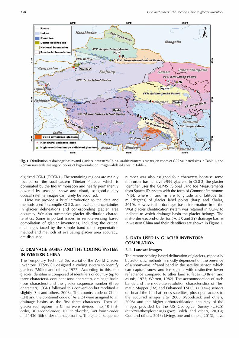
number was also assigned four characters because somefifth-order basins have >999 glaciers. In CGI-2, the glacieridentifier uses the GLIMS (Global Land Ice Measurementsfrom Space) ID system with the form of GnnnnnnEmmmmm[N|S], where n and m are longitude and latitude (inmillidegrees) of glacier label points (Raup and Khalsa,2010). However, the drainage basin information from theWGI glacier identification system was retained in CGI-2 toindicate to which drainage basin the glacier belongs. Thefirst-order (second-order for 5A, 5X and 5Y) drainage basinsin western China and their identifiers are shown in Figure 1.

3. DATA USED IN GLACIER INVENTORYCOMPILATION

3.1. Landsat imagesThe remote-sensing based delineation of glaciers, especiallyby automatic methods, is mostly dependent on the presenceof a shortwave infrared band in the satellite sensor, whichcan capture snow and ice signals with distinctive lowerreflectance compared to other land surfaces (O’Brien andMunis, 1975; Warren, 1982). The accommodation of suchbands and the moderate resolution characteristics of The-matic Mapper (TM) and Enhanced TM Plus (ETM+) sensorson board the Landsat series satellites, plus open access tothe acquired images after 2008 (Woodcock and others,2008) and the higher orthorectification accuracy of theimages provided by the US Geological Survey (USGS)(http://earthexplorer.usgs.gov/; Bolch and others, 2010a;Guo and others, 2013; Livingstone and others, 2013), have

Fig. 1.Distribution of drainage basins and glaciers in western China. Arabic numerals are region codes of GPS-validated sites in Table 1, andRoman numerals are region codes of high-resolution image-validated sites in Table 2.

Guo and others: The second Chinese glacier inventory358

made them the most popular source for glacier inventorycompilation (e.g. Aniya and others, 1996; Sidjak andWheate, 1999; Narama and others, 2006; Paul and others,2011a; Rastner and others, 2012). The CGI-2 also adopts theLandsat series images to delineate glaciers.

Figure 2a and b show the temporal distribution of Landsatscenes used in CGI-2. In total, 126 Landsat scenes areneeded to cover the glacierized regions of China. However,persistent snow and cloud cover in some regions made itdifficult to delineate glaciers from a single Landsat image, soauxiliary images were needed. This led to the use of a total of218 Landsat scenes in CGI-2. The scan line corrector (SLC)failure of ETM+ in 2003 seriously reduced image usability,and the ETM+ images were mostly used as auxiliary data.Most of the images used (�89%) were acquired by TM. Thetime span of the images was 2004–11, with �63% of thembeing taken in 2007 and 2009 and �92% during 2006–10.By area, the proportions of glaciers delineated are 23% in2007, 32% in 2009 and 26% in 2010. The absence of TMimages in 2008 was due to the lack of Chinese territorial dataon USGS websites (http://earthexplorer. usgs.gov/).

Glaciers in China are divided into those of continentaltype, whose greatest accumulation occurs during winter,and those of maritime type with strong summer accumu-lation (Shi and Li, 1981; Huang, 1990). The maritimeglaciers are mainly distributed in the southern and easternTibetan Plateau, and commonly have extensive snow andcloud cover during their ablation seasons. This leads toseasonal dispersion in the distribution of images, some ofwhich (14%) were taken during winter (November toMarch). However, most images were acquired duringablation seasons (April to October proportion is 86%), with�68% of scenes acquired around the end of ablationseasons (July to September), while the real glacier acquisi-tion season is concentrated in August (30% of total area) andSeptember (38%) (see Fig. 2b).

The accuracy of glacier delineation is mostly determinedby seasonal snow around the glacier or within the debris-covered area, and by cloud cover over the glacier surface.To give an overview of the quality of Landsat images used,we use a value of 2.0 as the threshold for TM3/TM5 todifferentiate snow within a five-pixel buffer of the glacieroutline and debris-covered area (>2.0), and cloud within theclean-ice area (<2.0). The ratio of snow- and cloud-coveredarea to the total area of all glaciers and their buffers withinthe image was regarded as the proxy of image quality. Theresults show that 86% of images have <20% snow/cloud

coverage, while �48% of images have <10% (Fig. 2c). Allthe selected ETM+ images have <20% cloud/snow cover-age. The spatial distribution of image quality (Fig. 2d and e)shows that the lower-quality images (snow/cloud coverage>20%) are mainly concentrated in the western Himalayaregion (30–32°N, 77–81° E) and Kunlun mountains (36°N),whereas the inland Tibetan Plateau (33–35°N, 84–90°E) hasthe best image quality.

3.2. Digital elevation modelsTwo kinds of digital elevation models (DEMs) were usedduring compilation of CGI-2. Delineations of the ice dividewere based on DEMs (cell size 30m) generated fromdigitized topographic maps, 1152 of which were 1 : 50 000scale and 348 of which were 1 : 100 000, which weremainly constructed from aerial photographs acquired duringthe 1950s–80s. A rigorous seven-coefficient transformationwas performed on the digitized contours and elevationpoints before DEM generation, to minimize potential errorsintroduced by mismatch of different coordinate systemsbetween Landsat images and topographic maps, where thecoefficients were calculated from coordinates of nationaltrigonometric stations within and around those mapscollected from the National Administration of Surveying,Mapping and Geoinformation of China. The Shuttle RadarTopography Mission (SRTM) DEM from the ConsultativeGroup for International Agriculture Research (CGIAR),version 4, where voids were filled using different auxiliaryDEMs (http://srtm.csi.cgiar.org), was used to derive glaciertopographic attributes. The reasons for such DEM choicesare described in Sections 4.2 and 7.3.

4. METHODS OF COMPILING GLACIERINVENTORY4.1. Glacier delineationBand ratio segmentation is the most robust and effectivemethod of glacier classification (e.g. Paul, 2001; Paul andothers, 2009; Racoviteanu and others, 2009). Duringcompilation of CGI-2, this method was adopted as a firststep to delineate glaciers. Manual improvements afterautomatic delineation are considered essential, especiallyin the case of lower image quality (e.g. Racoviteanu andothers, 2009; Paul and others, in press). The lower imagequality in many regions of western China required agreat deal of manual work to improve the accuracy ofglacier delineation, resulting in several rounds of manual

Fig. 2. Spatio-temporal characteristics and qualities of Landsat scenes used, and dates of glaciers in CGI-2.

Guo and others: The second Chinese glacier inventory 359

improvements during compilation of CGI-2. The manualimprovements were accomplished in the ArcMapworkbenchof the widely used ArcGIS software. In total, 12 participantswere asked to take part in this work after in-depth trainingsessions on the pixel-mixing mechanisms and correct glacierdiscrimination from Landsat images of varying quality.However, the final check and improvements were performedby only five participants, who were constantly involved for>3 years in compiling CGI-2 and were experienced in glacierdelineation. The excellent three-dimensional rendering ofGoogle EarthTM, along with its high-resolution images, cangreatly facilitate discrimination of glacier ice from seasonalsnow, cast shadow and, especially, debris-covered ice fromsurrounding moraines. During manual improvements,Google Earth™ image references via a plug-in of ArcMap(Export to KML) were found essential.

Several algorithms to automatically delineate debris-covered glaciers have been tested (e.g. Taschner and Ranzi,2002; Paul and others, 2004; Bolch and others, 2007; Shuklaand others, 2010). However, the low accuracy of their resultsobstructs their wider application, and it is recommended thatthey be used only as starting points for manual delineations(Paul and others, 2009, in press). Thus, delineation of debris-covered ice in CGI-2 was entirely based on manual digitiz-ation, as in most earlier studies (Hall and others, 1992;Racoviteanu and others, 2008, Burns and Nolin, 2014).Manual digitization of debris-covered glaciers was mainlybased on the recognition of distinctive surface features suchas supraglacial lakes, the outlets of subglacial streams nearglacier termini, and the landforms and drainage systems oflateral moraine, relying on the difference of surface coloursand textures in different red, green, blue composites ofLandsat images. The proper discrimination of debris-coveredglaciers depended on the above features and was animportant theme during the training of inventory participants.

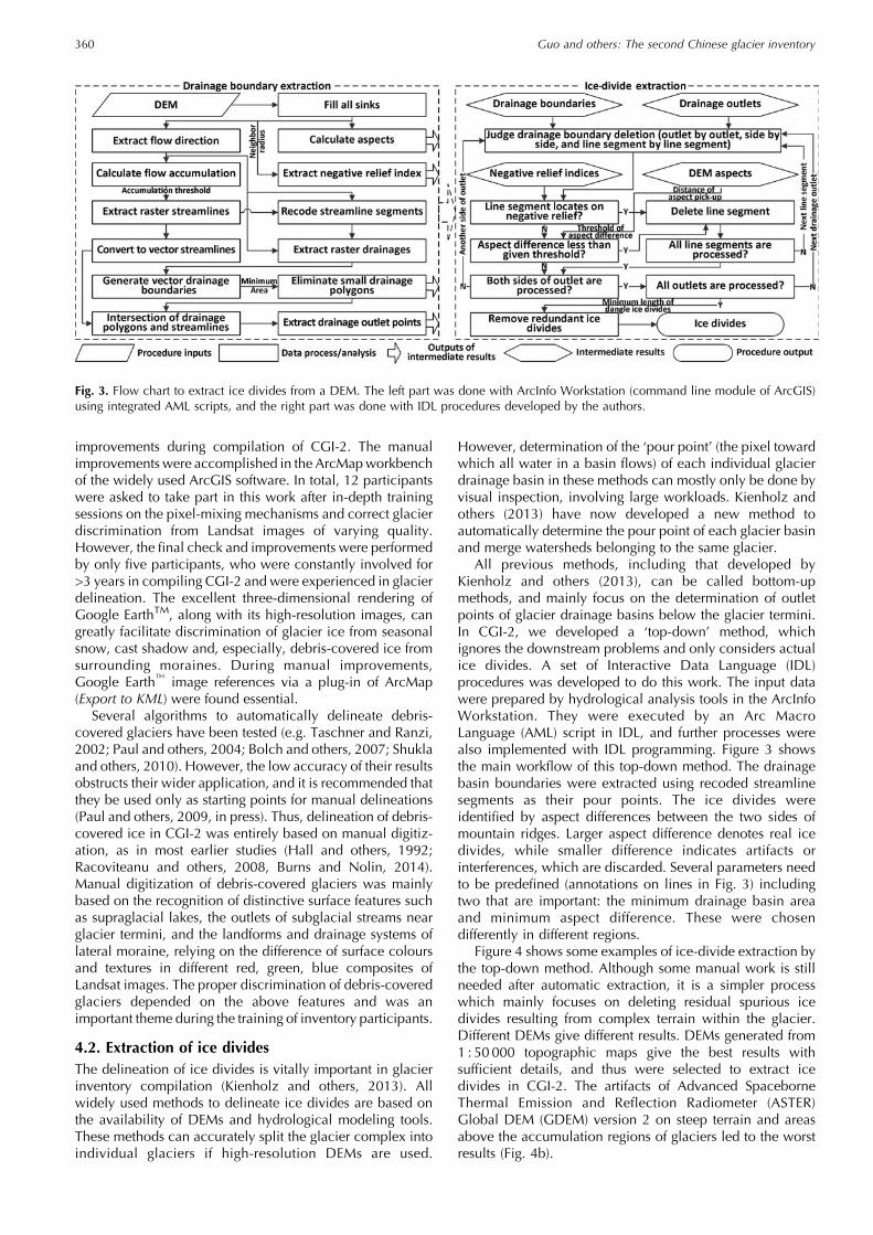
4.2. Extraction of ice dividesThe delineation of ice divides is vitally important in glacierinventory compilation (Kienholz and others, 2013). Allwidely used methods to delineate ice divides are based onthe availability of DEMs and hydrological modeling tools.These methods can accurately split the glacier complex intoindividual glaciers if high-resolution DEMs are used.

However, determination of the ‘pour point’ (the pixel towardwhich all water in a basin flows) of each individual glacierdrainage basin in these methods can mostly only be done byvisual inspection, involving large workloads. Kienholz andothers (2013) have now developed a new method toautomatically determine the pour point of each glacier basinand merge watersheds belonging to the same glacier.

All previous methods, including that developed byKienholz and others (2013), can be called bottom-upmethods, and mainly focus on the determination of outletpoints of glacier drainage basins below the glacier termini.In CGI-2, we developed a ‘top-down’ method, whichignores the downstream problems and only considers actualice divides. A set of Interactive Data Language (IDL)procedures was developed to do this work. The input datawere prepared by hydrological analysis tools in the ArcInfoWorkstation. They were executed by an Arc MacroLanguage (AML) script in IDL, and further processes werealso implemented with IDL programming. Figure 3 showsthe main workflow of this top-down method. The drainagebasin boundaries were extracted using recoded streamlinesegments as their pour points. The ice divides wereidentified by aspect differences between the two sides ofmountain ridges. Larger aspect difference denotes real icedivides, while smaller difference indicates artifacts orinterferences, which are discarded. Several parameters needto be predefined (annotations on lines in Fig. 3) includingtwo that are important: the minimum drainage basin areaand minimum aspect difference. These were chosendifferently in different regions.

Figure 4 shows some examples of ice-divide extraction bythe top-down method. Although some manual work is stillneeded after automatic extraction, it is a simpler processwhich mainly focuses on deleting residual spurious icedivides resulting from complex terrain within the glacier.Different DEMs give different results. DEMs generated from1 : 50 000 topographic maps give the best results withsufficient details, and thus were selected to extract icedivides in CGI-2. The artifacts of Advanced SpaceborneThermal Emission and Reflection Radiometer (ASTER)Global DEM (GDEM) version 2 on steep terrain and areasabove the accumulation regions of glaciers led to the worstresults (Fig. 4b).

Fig. 3. Flow chart to extract ice divides from a DEM. The left part was done with ArcInfo Workstation (command line module of ArcGIS)using integrated AML scripts, and the right part was done with IDL procedures developed by the authors.


4.3. Attributes for individual glaciersAccording to the old guidelines of WGI (UNESCO/IASH,1970; Müller and others, 1977), many attributes of a glacierneed to be assigned in the glacier inventory, includingglacier name, drainage basin ID, source material, area,width, length, elevation, classification, etc. In remote-sensing- and GIS-based compilation of glacier inventories,some of these attributes still require much manual proces-sing and glaciological expertise, so the latest guidelines forremote-sensing-based glacier inventories (Paul and others,2010) recommend delayed assignment of several attributessuch as glacier name, WGI code, clean-ice area, classifi-cation, etc., for quick compilation of glacier inventories inthe GLIMS framework.

In CGI-2, we assigned most attributes recommended byPaul and others (2010) except glacier length. Someresearchers have developed several algorithms to auto-matically extract glacier center lines for glacier lengthcalculation (e.g. Le Bris and Paul, 2013; Kienholz andothers, 2014; Machguth and Huss, 2014). However, theautomatically extracted glacier center lines also requiremanual improvements. The large number of glaciers in

China makes such work time-consuming, so currently theglacier length has not been assigned.

Most of the assigned attributes were calculated usingmethods similar to those suggested by Paul and others(2010). The glacier areas were calculated in an Albersequal-area conic projection with standard parallels at 25°Nand 47°N. The label points of glacier polygons weregenerated automatically in ArcInfo Workstation (procedureCreateLabels) and checked by visual inspection one by one.Points close to the glacier outline were relocated to betterrepresent the glacier location. The source image attributewas divided into two fields, i.e. the primary image and theauxiliary image, while the representative date of the glacierwas only derived from the primary source.

As mentioned in Section 3.1, the topographic attributeswere calculated based on SRTM version 4. To avoidinaccurate cell exclusion and inclusion when masking theDEM with the glacier outline, the SRTM DEM wasresampled into the same resolution as TM (30m) using thebilinear interpolation method. The maximum, minimum andmean elevations were then extracted from statistics of allresampled SRTM DEM cells located within the glacier

Fig. 4. Ice divides in Anyemaqen mountains, Qinghai Province, extracted from (a) SRTM, (b) GDEM2 and (c) 1 : 50 000 topo-DEM. Theintersected and modified ice divides in (c) are shown in (a) and (b) for comparison. The other examples are ice divides extracted from1 : 50 000 topo-DEMs for (d) Gongga mountains, Sichuan Province, (e) Purogangri, Tibet Province, and (f) Bogda mountains, XinjiangProvince. MBA and MAD are the minimum basin area and minimum aspect difference, respectively.


outline, while the median elevation was extracted as the50th percentile of the cumulative number distribution of cellelevations. The mean slope was simply determined by theaverage value of slope across all cells. The mean aspect wascalculated by dividing the mean sine by the mean cosine ofaspect across all cells (Paul and others, 2010).

5. ERROR ASSESSMENTS

5.1. Methodological accuracy of glacier delineationGLIMS has conducted several experiments to reveal theuncertainties in glacier inventory compilation using differentmethods (GLACE 1 and GLACE 2; Raup and others, 2007).The sources of glacier delineation errors can be divided intothree classes (Raup and others, 2007; Paul and Andreassen,2009): technical errors, interpretation errors and methodo-logical errors. Technical errors can be mostly ignored if thesatellite image has been accurately orthorectified, whichwas the case for Landsat images provided by USGS (e.g.Bolch and others, 2010a; Guo and others, 2013). Interpret-ation errors mostly depend on how ‘glacier’ is defined forthe purposes of inventory compilation, and thus are difficultto evaluate. Methodological errors were largely decided bythe resolution of the Landsat images, and the skills of theinventory compilers which also cannot accurately beassessed (Pfeffer and others, 2014). In the case of CGI-2,the GLIMS guidelines (Racoviteanu and others, 2009; Pauland others, 2010) were followed to minimize interpretationerror, and the compilers were well trained to enhance theirskills. However, the glacier mapping error still needs to beproperly evaluated. This was done by incorporating all errorsources into one term, i.e. methodological errors, whichwere determined by comparing the glacier outlines with theglacier marginal positions measured during field GPSinvestigation, and the glacier outlines delineated fromhigh-resolution Google MapsTM images.

Many real-time kinematic differential GPS (RTK-DGPS)measurements (Unistrong E650 GPS instruments) wereobtained during field investigations in 2007–08 (Shangguanand others, 2008, 2010; Li and others, 2010), which alsoincluded many measurements of glacier boundaries. Thesemeasurements have very high accuracy (�0.1 to �0.3m)compared to the coarse spatial resolution of Landsat images

used in CGI-2. However, the GPS measurement datesmostly differ from the acquisition dates of the best imagesselected to compile the glacier inventory in these regions.We use the GPS measurements to evaluate the positioningaccuracy of glacier outlines delineated from Landsat imageswith dates as close as possible to the GPS measurementdates. The same delineation methods were used as incompiling CGI-2 (see Fig. 5 for examples). Other errors (e.g.mis-registration of Landsat images or incorrect recognitionof boundaries of debris-covered glaciers during field investi-gation) may also be significant, but our GPS–Landsatcomparisons give an overview of the methodologicalaccuracy in glacier inventory compilation.

In total, 23 glaciers (see Fig. 1 for the distribution ofmeasured glaciers) were measured by RTK-DGPS, with>2320 measurements located on the glacier margins(Table 1). Landsat images of acceptable quality and withsimilar acquisition dates to the GPS measurements (max-imum difference �1 year) were downloaded from the USGSwebsite.

Table 1 shows the results of comparisons between GPSmeasurements and delineated glacier outlines. The accuracyis ��18m for automatically delineated and ��11m formanually improved glacier outlines, while the accuracy ofmanually delineated outlines of debris-covered ice is in theorder of �30m.

In addition to the field RTK-DGPSmeasurements, we usedhigh-resolution satellite images to validate the accuracy ofthe glacier delineation methods in CGI-2 (see Fig. 6 for atypical case), as in previous studies (Paul and others, 2013).The high-resolution screenshots of Google MapsTM werecaptured for seven randomly selected regions (see Fig. 1 fortheir distribution), where higher-resolution images in GoogleMapsTM and nearly simultaneous Landsat images areavailable. Only images with a spatial resolution better than1m in Google MapsTM were selected. The glacier outlines onthe screenshots of Google MapsTM were manually digitizedand regarded as the ground truth. They were then comparedwith automatically extracted and manually improved glacieroutlines from nearly simultaneous Landsat images. Thedebris-covered glaciers were also manually digitized fromboth kinds of images. The offsets between Landsat andGoogle Maps™ outlines were calculated as the distancesbetween points taken every 10m along the Landsat outline

Fig. 5. Examples of glacier outline accuracy assessments by field RTK-DGPS measurements: (a) central Qilian mountains (RC1 in Fig. 1 andTable 1; glaciers No. 1 and No. 5 in Shuiguan river basin); (b) western Qilian mountains (RC3; Laohugou glacier No. 12); and (c) centralTien Shan (RC8; Fenliu glacier, Bogda peak).


and the nearest points on the corresponding Google Maps™

outline. The glacier area differences between the two sets ofresults were also calculated (Table 2).

The results of high-resolution image validation in Table 2give offsets similar to those in Table 1. The average offsetsalso suggest better accuracy after manual improvement(11.37m vs 17.03m). The uncertainties in debris-coveredglacier outline delineation are still high in this validation,illustrating the difficulties of accurate delineation of debris-covered glacier outlines.

5.2. Glacier area error assessmentThe glacier area error tends to be inversely proportional tothe length of the glacier margin (Pfeffer and others, 2014), soit depends strongly on the size of the glacier (larger glaciersmostly have longer margins). In this sense, the area errorassessed by glacier buffers (Granshaw and Fountain, 2006;Bolch and others, 2010a) is rational because it accounts forthe length of the glacier perimeter. The buffer width,however, is critical to the resultant glacier area error.

The area error assessment of CGI-2 uses a method similarto the buffer method suggested by Rivera and others (2005),

and includes both the length of glacier outlines and theirpositioning accuracies. The above assessments of methodo-logical accuracy suggest ��10m and ��30m for clean-iceand debris-covered glacier outline delineation, respectively.Regarding the mis-recognition of glacier boundaries in thefield and mis-registration of satellite images, as well as theinfluence of seasonal snow remnants, we consider the�10m and �30m accuracies for clean-ice and debris-covered glacier outlines as a reasonable basis for evaluatingtheir area error. The boundaries between clean-ice anddebris-covered ice were mostly not manually improved, sotheir positioning accuracy was regarded as �15m, a valueused by some researchers (e.g. Bolch and others, 2010a;Rastner and others, 2012). As described in Section 4.2, thedelineation of ice divides is vitally dependent on the DEMused, so their accuracy is difficult to evaluate. In CGI-2, weused the DEM pixel size (30m for 1 : 50 000 topo-DEM usedin CGI-2) as the positioning accuracy of ice divides in areaerror calculations. The area error evaluations in CGI-2 werethen calculated using

EA ¼ LcEpc þ LdEpd þ LiEpi ð1Þwhere EA is the glacier area error, Lc, Ld and Li are the length

Table 1.Offsets (m) between field GPS measurements and glacier outlines delineated by the methods of CGI-2. RC is region code, M-Date isdate of GPS measurements, A-Date is date of Landsat image acquisition, NG is number of surveyed glaciers, NP is number of measuredboundary GPS points, STD is standard deviation, and the prefixes A- and M- indicate automatically extracted and manually improvedglacier outlines, respectively

RC M-Date / A-Date NG Clean ice Debris-covered ice

NP A-Mean A-Max A-STD M-Mean M-Max M-STD NP Mean Max STD

1 Jul 2007 / 6 Jul 2007 4 244 39.8 297.2 69.4 8.3 42.5 7.3 201 31.4 162.6 29.82 Aug 2007 / 12 Aug 2007 2 197 14.0 40.9 9.9 13.0 39.0 9.3 60 13.8 56.1 13.93 Jul 2007 / 27 Aug 2007 1 465 11.1 55.5 9.8 11.3 56.7 9.0 69 12.1 40.2 9.04 Oct 2007 / 30 Jul 2006 4 158 14.1 51.3 11.4 12.6 43.3 9.7 37 17.3 45.9 13.75 Oct 2007 / 5 May 2007 2 153 23.2 100.2 20.8 7.6 23.5 5.2 – – – –6 May 2008 / 7 Aug 2008 3 7 10.0 18.3 5.4 10.5 17.7 6 101 41.9 100.9 27.77 Jun 2008 / 24 Aug 2007 3 12 5.2 11.1 3.3 5.5 13.2 4.9 332 39.6 141.4 29.98 Jul 2008 / 24 Aug 2008 4 221 13.4 111.6 14.5 11 70.4 9.3 66 16.9 41.9 12

Total/Summary* 23 1457 18.2 297.2 21.8 10.7 70.4 8.4 866 31.3 162.6 24.8

*Calculations of summary values of Mean and STD were weighted by measured point counts.

Fig. 6. Example of glacier outline accuracy assessment via screenshot of Google Maps™ (RC I in Fig. 1 and Table 2).


of clean-ice, debris-covered glacier outlines and ice divides,respectively, and Epc , Epdand Epi are their positioningaccuracies.

Equation (1) was used in area error calculations for everyindividual glacier. The errors at boundaries between cleanand debris-covered ice make no contribution to the error ofthe whole glacier area. At drainage-basin and larger scales,the errors at interior ice divides are also omitted. Theresulting glacier area errors of the 15 basins and the wholeof CGI-2 are shown in Table 3. The area error of allcompiled glaciers in CGI-2 was �3.2%. The largest areaerror was �8.6% in the Keboduo river basin (5Y124), whichonly has 0.8 km2 of glaciers. The errors of debris-covered

areas were much larger than those of whole glacier areas,amounting to �17.6% for all debris-covered ice in CGI-2.

6. RESULTS

6.1. General results of CGI-2In total, 42 370 glaciers were compiled in the current CGI-2,with a total area of �43 087 km2 (Table 3). The minimumarea of glaciers compiled is 0.01 km2. About 59% of thecompiled glaciers are distributed in the Ganges river basinand Tarim inland basin, and 16% are distributed in TibetanPlateau inland basins. The current compiled glaciers in

Table 2. Offsets (m) of glacier outlines that were automatically delineated and manually improved from Landsat images compared withoutlines manually digitized from high-resolution screenshots of Google MapsTM. RC is region code, H-Date is acquisition date of GoogleMapsTM images and L-Date is date of Landsat images

RC H-Date L-Date Clean ice Debris-covered ice

Area* Length* Automatic Manual Area* Length* Area diff Mean offset

Area diff Mean offset Area diff Mean offset

I 11 Sep 2007 18 Sep 2007 6.36† 127.89 3.9 12.45 0.5 9.67 0.03 7.39 59.3 17.26II 12 Aug 2010 20 Aug 2010 5.7† 68.4 4.7 12.37 –3.4 11.63 0.23 8.3 35.8 31.81III 18 Oct 2009 9 Aug 2009 – 56.78 – 15.70 – 7.92 – 1.0 – 28.22

7 Aug 2003IV 16 Oct 2003 23 Aug 2003 – 36.79 – 14.27 – 9.09 – – – –V 18 Oct 2007 8 Jul 2007 1.4† 69.9 –6.4 14.71 –3.6 11.50 – – – –

14 Nov 2007VI 16 Oct 2012 22 May 2007 17.73 98.73 5.8 18.94 3 11.33 – – – –

7 Jun 2007VII 5 Apr 2011 18 Oct 2011 26.3 97.7 6.1 20.87 1.6 12.31 – – – –

Total/Summary 57.49† 556.14 5.4 17.03 1.3 11.37 0.26 16.63 38.3 26.12

*The values are for investigated glaciers digitized from high-resolution screenshots of Google MapsTM.†The area (km2) is only calculated for glaciers whose outlines were not obscured by seasonal snow, and the area differences and mean offsets are calculated by

Table 3. Glacier distributions in different drainage basins of western China from CGI-2, and their comparisons to CGI-1 and DCGI-1. R.indicates river, and I.B. inland basins

Drainage basin Area of CGI-1* Area of DCGI-1 All area of CGI-2 Debris-covered area of CGI-2

Name Code All glaciers CGI-2 unfinished Number Area Uncertainty Number Area Uncertainty

km2 km2 km2 km2 % km2 %

Irtysh R. 5A2 289 293.4 – 279 186.1 4.9 10 1.2 53.8Yellow R. 5J 173 172.3 – 164 126.7 3.6 5 2.4 30.5Yangtze R. 5K 1895 1907.1 133.5 1378 1541.3 3.2 25 30.4 16.5Mekong R. 5L 316 324.5 0.9 465 230.4 5.0 3 0.1 54.9Salween R. 5N 1730 1729.8 778.3 1361 700.7 4.9 7 1.7 32.1Ganges R. 5O 18102 18 437.0 7840.0 7420 7881.6 3.5 295 402.7 15.8Indus R. 5Q 1451 1402.1 – 2404 1107.1 5.5 42 11.8 35.7Ili R. 5X0 2023 2050.0 – 2121 1554.4 4.8 198 76.8 26.6Keboduo R. 5Y124 3 2.7 – 4 0.8 8.6 – – –Hexi I.B. 5Y4 1335 1394.4 – 2056 1072.7 4.8 12 1.1 54.9Qaidam I.B. 5Y5 1865 1967.6 – 2073 1775.6 3.4 2 0.8 19.2Tarim I.B. 5Y6 19 878 20 424.4 – 12 795 17724.6 3.1 1034 950.8 16.8Junggar I.B. 5Y7 2251 2390.5 – 3096 1737.3 5.1 81 12.1 47.6Turpan-Hami I.B.

5Y8 253 265.1 – 378 178.1 6.0 2 0.6 44.3

TibetanPlateau I.B.

5Z 7836 8035.6 0.6 6376 7269.4 2.7 7 1.2 56.0

Total 59 400 60 796.5 8753.3 42 370 43086.8 3.2 1723 1493.7 17.6

*Numbers in this column are taken from the corresponding basins list in Shi and others (2008, p. 42). The basin 5X1 (Karakul Lake) is not included as it wasomitted from CGI-2 due to national boundary changes.


CGI-2 correspond to a total area of �52 043 km2 of glaciersin DCGI-1 (�86% of the total). Approximately 90% of thearea (7840 km2 from DCGI-1) of uncompiled glaciers islocated in the Ganges river basin, while 9% and 1% are inthe Yangtze and Salween river basins, respectively.

A general feature of glacier size distributions is that largenumbers of small glaciers account for a small proportion oftotal area, and a lesser number of larger glaciers account formost of the total area (Paul and Svoboda, 2009; Le Bris andothers, 2011; Bliss and others, 2013; Hagg and others, 2013).This feature is also very clear in China. The distribution ofglaciers of different sizes is shown in Figure 7. Most glaciers(�83% of the total) have an area of <1 km2 (Fig. 7c), and only�3% of glaciers have an area larger than 5 km2. However,the total area occupied by glaciers smaller than 1 km2 onlyamounts to 20% of the total CGI-2 area (Fig. 7d), whileglaciers larger than 5 km2 occupied 51% of the area.

The distribution of glaciers within different area classes indifferent drainage basins (Fig. 7c) exhibits similar patterns toTable 3. However, the number and area of glaciers of eacharea class are different in each drainage basin. The numberproportion of glaciers smaller than 1 km2 is close to 80% inmost drainage basins, but is very high (�90%) in theSalween river (5N), Indus river (5Q) and Turpan–Hamiinland basins (5Y8), which means that these three drainagebasins have more small glaciers. Glaciers larger than 5 km2

are concentrated in the Ganges river (5O), Tarim basin (5Y6)and Tibetan Plateau inland basins (5Z) (amounting to 17%,47% and 19% of the total area of >5 km2 glaciers in CGI-2,respectively). Glaciers larger than 50 km2 are also concen-trated in these three drainage basins (amounting to 97% ofthe total area of all >50 km2 glaciers), while all glacierslarger than 100 km2 are located within these basins,including the largest glacier in CGI-2, Insukati glacier(359 km2) in Tarim basin. On the other hand, the larger

area proportions of glaciers smaller than 1 km2 in theSalween river (5N), Indus river (5Q), Turpan-Hami inlandbasins (5Y8), Mekong river (5L), Hexi (5Y4) and Junggarinland basins (5Y7) indicate that more glaciers in these sixbasins are small glaciers. The lower area proportions of>5 km2 glaciers in these six basins also illustrate thedominance of small glaciers.

6.2. Glacier hypsographyGlacier hypsography can provide useful information forunderstanding the regional topography, geomorphology andclimate (Meier and others, 2007). Figure 8b shows theglacier hypsography with 100m elevation intervals of 14larger mountain systems in western China (Fig. 8a). About57% of the glacier area is distributed in the 5000–6000melevation range, while 26% is located below 5000m, andonly 17% above 6000m.

For the elevation of maximum glacier area distribution,an overall south-to-north trend of slight increase followed bysharp decrease can be identified from Figure 8b. The highestmodal elevation (most heavily glacierized) appears in theGangdise mountain range (�5900m). The modal elevationshows a slight increase from the Himalaya range (�5800m)to the Gangdise range. Then it retains this level of �5900mto the Qiangtang plateau, Karakoram mountain range andKunlun range, and decreases sharply northwards from theTien Shan and the Saur range to the Altai. The Altaimountains have the lowest glaciers in China (minimumelevation 2360m).

Two overall west-to-east descending trends of the modalelevation can also be identified from Figure 8b. The firstdescending trend is located along the southern TibetanPlateau, where the modal elevations decrease from theGangdise range to the Nyenchen Tanglha mountain range(�5830m) and then to the Hengduan mountain range

Fig. 7. Total glacier numbers (a) and area (b) of CGI-2 and their respective proportions (c, d) within different area classes and differentdrainage basins.


(�5440m). Another west-to-east descending trend is locatedalong the northern edge of the Tibetan Plateau, where thehighest modal elevation is �5890m at the Kunlun,descending to �5290m at the Altun and then to �4980mat the Qilian. The bimodal glacier hypsography of theKunlun mountains is explained by the concentrations ofthree large glacier centers. The first center, located on thewest Kunlun mountain range, has a mean elevation>5800m, and the glacier area occupies nearly one-tenthof CGI-2. The other two centers, namely Muztag peak (akaMuztagh Ata) and Xinqing peak, are located within thecentral and eastern Kunlun mountain ranges, with�1300 km2 of glaciers and mean elevations of �5400m.

6.3. Distribution of glaciers of different orientationFigure 9 shows the glacier area distributions within differentslope and aspect ranges in 14 mountain systems of westernChina and the whole of CGI-2, in which areas are calculatedby counting the number of glacier DEM cells in differentaspect and slope ranges rather than the mean slopes andaspects of all glaciers. The mean glacier surface slope ofCGI-2 is 19.9°. The Pamir plateau, Qilian mountain range,and Altun mountains have the steepest glacier surfaces,where �two-thirds or more of the glacier areas have asurface slope greater than 15°. By contrast, Qiangtangplateau and the Tanglha mountains have the gentlest glaciersurfaces, where more of the glacier areas are distributedbelow 15° (area proportions below 15° reaching 64% and59%, respectively). The glacier area distribution withindifferent aspect ranges also shows remarkable spatialdiscrepancies. An overall characteristic is the predominanceof north-northeast-facing glaciers with a mean aspect of24.3°. The proportions of north- (315–45°) and east-facing(45–135°) glacier areas are 39% and 28%, respectively.Glaciers in the Saur, Qilian, Altun and Gangdise mountainsshow very distinctive north-facing characteristics; the arealproportions of north-facing glaciers all exceed 50%. By

contrast, glaciers in the Karakoram mountains, Qiangtangplateau and Hengduan mountains show the dominance ofnortheast facing, where the proportions of north- and east-facing glacier areas all exceed 30%.

Analysis of the orientation of different glacier sizes showsthat smaller glaciers (<2 km2) are more likely to be locatedon north-facing slopes (area proportion 56%), while largerglaciers are more evenly distributed on north- and east-facing slopes (the area proportion of east-facing glacierslarger than 2 km2 amounts to one-third versus one-fifth ofglaciers smaller than 2 km2). The glaciers larger than 5 km2

in the Tien Shan, Karakoram, Gangdise, Hengduan andNyenchentanglha mountains and the Pamir and Qiangtangplateaus are mostly distributed on the east- rather thannorth-facing slopes. By contrast, most of the glacier area inthe Kunlun, Qilian and Altun mountains tends to bedistributed on north-facing slopes.

6.4. Distribution of debris-covered glaciersIn total, 1723 glaciers are covered by 1493.7 km2 of debrisin CGI-2 (Table 3). The average ratio of debris-covered areato total glacier area for these glaciers is 12%. Glaciers withdebris-covered area are mostly concentrated in five centers:Tumur peak, Tien Shan; eastern Pamir plateau; Karakoram;the Himalaya; and Gangrigabu peak, Nyenchen Tanglhamountains (see Fig. 1 for distribution of debris-coveredglaciers). Tumur peak is the largest debris-covered glaciercenter. The area of debris-covered ice in this region amountsto 29% (430 km2) of the total area of debris-covered ice inCGI-2, and accounts for 14% of the total area of debris-covered glaciers in this region. The two largest debris-covered glaciers in China are located on Tumur peak.Tumur glacier, which has the largest debris-covered area inCGI-2, has a debris area of 63 km2 (�17% of its total area),and the debris extends to 4520ma.s.l. (�two-fifths of theglacier’s elevation range, 2890–7030m). The second-largestdebris-covered glacier is Tugbelqi glacier, which has a

Fig. 8. Mountain systems defined in CGI-2 (a) and their glacier hypsography (100m elevation interval) (b). Gray lines in (b) are the medianelevations of all inventoried glaciers in corresponding mountain regions. Note that in (b) the scale on the horizontal axis differs from regionto region.


debris area of 39 km2 (13% of its total area), and the highestelevation of debris is 4267m (also �two-fifths of theglacier’s elevation range).

The Himalaya and the eastern Pamir plateau are twoother major centers of debris-covered glaciers. About 19%(283 km2) of debris-covered area is distributed in theHimalaya, of which �70% (199 km2) is distributed inregions around Qomolangma (Mount Everest), Lapche Kangand Shishapangma. The eastern Pamir plateau is the third-largest center of debris-covered glaciers, with a total debris-covered area of 207 km2 (14% of CGI-2). Most (�65%;134 km2) of the debris-covered area in this region isdistributed on Kongur Tagh and Muztagh Ata.

7. DISCUSSION7.1. Glacier delineationThe band ratio segmentation method proved robust and effi-cient when the best-quality imagery was available. Ourmethod experiments also revealed the insensitivity of theband ratio segmentation method to the band ratio thresholdswhen high-quality satellite imagery is used and on gentlerterrain (Fig. 10a and b). The generally achievable discrimina-tion of 0.1 on the band-ratio threshold in the range 1.0–3.0will only result in an area difference of �0.1 km2 (100 km)–1.This will lead to an area error of��0.3%, assuming a typicalperimeter/area ratio of �3 kmkm–2 (the mean from CGI-1).However, as illustrated by Racoviteanu and others (2009),the fully automatic glacier outline delineation using thismethod was often obstructed by numerous factors, especiallywhen image quality was poor, and in regions with larger

elevation differences where strongly ablating areas on glaciertongues commonly coexist with melting snow remnantsclose to or above the equilibrium line, or in areas with thinclouds or shadows (Fig. 10c and d). Such regions are verycommon in western China, and such confounding factorscan usually only be resolved by manual digitization, re-quiring many hours of work. The absolute determination of apixel as either glacier or non-glacier is another shortcomingof the band ratio segmentation method, which has beenshown to underestimate the glacier area by excluding mixedpixels (Paul and others, 2013). This issue also arises whenusing other automatic classification methods.

In contrast to automatic glacier delineation methods,manual digitization can partly solve the problems induced byseasonal snow and can discriminate the ice in mixed pixels.However, Paul and others (2013) revealed larger uncertain-ties in manual glacier outline delineation. This study illus-trated that the accuracy of manual work is vitally dependenton the experience of participants in correctly discriminatingglacier and non-glacier pixels, and on their skill in identifyingpossible ice in mixed pixels along glacier outlines. Since thecompilers of any one glacier inventory may vary greatly intheir levels of experience and knowledge, manually im-proved or digitized glacier outlines by different participantscan show very large differences (in order of 5–10%; Paul andothers, 2011a), even in repeated digitization by the sameparticipants. However, the lower image quality in manyregions of western China requires many hours of manualwork. To minimize the errors induced by insufficientexperience and knowledge of glacier delineation frommultispectral satellite images, participants were intensively

Fig. 9. Glacier area distribution within different surface slope (5° interval) and aspect (11.25° interval) ranges for 14 mountain systems inwestern China (Fig. 8a) and the whole of CGI-2. Black lines indicate the mean glacier surface slopes and aspects. The area values wereobtained by counting pixels in each slope and aspect range, and the mean slope and aspect were also calculated from all glacier pixels ineach mountain system.


trained before their real work began, and only those whowere constantly involved in glacier inventory compilationwere selected for the final revision of the glacier outlines.

7.2. Error assessmentsDirect evaluation of area errors by comparison with glaciersdelineated from high-resolution images (Paul and others,2011a, 2013) is likely to be affected by biases since the erroris strongly size-dependent when expressed as a fraction ofthe total area. We used a more straightforward method tobetter evaluate the accuracies of manually improved glacieroutlines, firstly assessing the positioning errors and thenusing them to evaluate the area errors. Some factors will alsointroduce uncertainties in the final glacier outline pos-itioning errors, including: (1) discrepancies between valid-ated outlines and real outlines of sampled glaciers in CGI-2,(2) mis-registration of satellite images, (3) incorrect recogni-tion of glacier margins (especially margins of debris-coveredice) during fieldwork or on higher-resolution images, and(4) the preference for field GPS measurements in theablation area. Of these factors, (2) and (3) will lead tooverestimation of positioning errors, while (4) will result inunderestimation. Furthermore, the selected validating pointswere aligned on both sides of referencing glacier outlines, inwhich different sides indicate different area errors (negativeor positive). In this sense, the mean offsets of all points usedin area error evaluation will result in overestimation.However, the selected �10m and �30m positioning errorthresholds for clean ice and debris-covered ice were thoughtto be reasonable if counting all these factors together.

The substantial impacts of manual improvements on thepositioning accuracy of automatically delineated glacieroutlines demonstrated the need for such improvement (Raup

and others, 2007). On the other hand, since no further co-registration was performed on either kind of satellite imageused, the small offsets between the three kinds of glacieroutline tend to confirm the acceptable orthorectificationaccuracy of Landsat images provided by USGS. This is alsodocumented by previous studies (Bolch and others, 2010a;Guo and others, 2013; Livingstone and others, 2013).

In contrast to clean-ice outlines, our accuracy assessmentfor outlines of debris-covered ice faces more challenges.Although it is much easier to distinguish these outlines usinghigh-resolution images, large uncertainties still exist be-cause, no matter what the resolution of the image, debris-covered ice is difficult to discriminate from adjacent moraineor rock slopes. Even in the field, the margins of buried iceunder debris covers are not always easily recognized(Haeberli and Epifani, 1986). However, since their validationis so difficult, the validations in this paper can providevaluable guidance on the accuracies we can achieve.

Besides glacier area errors, the assigned glacier attributes(e.g. maximum, minimum and median elevation, meanslope and aspect) must also contain some errors. However,these are more dependent on the accuracy and spatialresolution of the SRTM used. This accuracy could not beevaluated rigorously in the present study because ofinconsistencies between the acquisition dates of the SRTMand Landsat images used, and also the lack of in situmeasurements of glacier surface elevation.

7.3. DEM in CGI-2Both SRTM and ASTER GDEM were considered for theextraction of glacier topographic attributes (Paul and others,2010). However, although it has higher resolution, theexisting undulations and artifact-related roughness variations

Fig. 10. The insensitivity of glacier area to band ratio threshold selection in case of high image quality and gentle terrain (a, b), and a typicalcase of problematic determination of optimal band ratio threshold to delineate glaciers with TM3/TM5 (c) and TM4/TM5 (d) when usinglower-quality image and on rugged terrain. The sensitivity was tested within �500m buffers of glacier outlines (white loops in (a)) and bychange in thresholds with steps of 0.05, 0.1 and 0.2 (b). White rectangles in (c) and (d) denote regions where different thresholds givecontradictory results: (1) shadow, (2) thin cloud, (3) snow remnants and (4) glacier tongue. Date format is yyyy/m/dd.


in ASTER GDEM lead to very large differences (more than�500m; Frey and Paul, 2012), which can also be observedin Figure 4b. The broad range of acquisition dates due to thestacking of DEMs extracted from different ASTER scenes(Fujisada and others, 2012) is another limitation of GDEM fortopographic attribute calculations.

Although the data voids in steep terrain and under-estimation of surface elevation in the accumulation area dueto penetration of radar waves reduces its usability in glacierstudy, SRTM shows more uniform qualities within glacier-covered regions compared to ASTER GDEM, and has beenused in the compilation of several glacier inventories (e.g.Bolch and others, 2010b; Le Bris and others, 2011; Paul andothers, 2011b) and glacier change studies (e.g. Rignot andothers, 2003; Aizen and others, 2006; Bown and others,2008). Frey and Paul (2012) found that SRTM is slightlybetter than GDEM in the compilation of topographicattributes of glacier inventories. Many other studies (e.g.Zhao and others, 2010; Li and others, 2013) have alsoillustrated the greater accuracy of SRTM than GDEM inChinese territory. According to the above differencesbetween SRTM and GDEM, the calculation of elevationattributes in CGI-2 employs SRTM as the main DEM source.The results shown in Figures 8 and 9 illustrate its goodperformance in such activities.

7.4. Comparisons between glacier inventories ofChinaCGI-1 has often been cited in previous research. Itssubmission to the GLIMS database further promoted itssignificance in scientific work, and it was included in thenew RGI (Pfeffer and others, 2014). However, the glacieroutlines compiled into the RGI were mostly digitized from80 scanned digital copies of glacier inventory maps madeduring the compilation of CGI-1 (Wu and Li, 2004), whichwere concisely drawn from 1 : 50 000 and 1 : 100 000topographic maps and have scales ranging from1 : 100 000 to 1:1 000 000 (mostly 1 : 200 000 to1 : 400 000). Furthermore, the glacier area in the originalCGI-1 (total 59 425 km2; Shi and others, 2009) was entirelybased on manual measurements by planimeter and thusaffected by many artifacts. The data shown in Table 3provided detailed information about the differences be-tween the two versions of CGI-1. The glacier areas wereunderestimated by the original CGI-1 in most drainagebasins, with a total underestimation of 1397 km2.

By detailed visual inspection, we found large differencesbetween DCGI-1 and the current CGI-2, including theomission of some glaciers on topographic maps, largerdifferences in the acquisition dates of topographic mapsused in CGI-1, different definitions of glaciers on steepterrain of accumulation areas, and the determination ofdebris-covered areas. The apparent glacier change in China(–17.2%) can be read from Table 3 by subtracting thecorresponding CGI-1 area (52 043 km2) from the currentCGI-2 area (43 087 km2), and this change rate can beconsidered even larger (�17.9%) if we exclude CGI-2glaciers omitted by CGI-1 (�371 km2 total). However, suchchange analysis is not proposed since there are manydifferences between the DCGI-1 and current CGI-2.Furthermore, the image quality and glacier inventoryaccuracy of DCGI-1 will involve further work which isbeyond the scope of this paper. Detailed change analysiswill be introduced in a future paper.

7.5. About the unfinished part of the Chinesecontemporary glacier inventoryThe acquisition dates of Landsat images used to compileCGI-2 were originally planned to be confined to around2008 to ensure the glacier inventory represented a near-isochronous assessment of the status of glaciers in China.However, the SLC failure of the Landsat ETM+ sensor in2003, and the absence of TM images in 2008, significantlyinfluenced Landsat image availability and expanded therange of acquisition dates. Nevertheless, 90% of our imagesare from 2006–10.

More than one-fifth of glaciers in China are distributed inthe southeastern Tibetan Plateau. However, this region wasalmost permanently covered by snow and cloud due to theinfluence of the Indian monsoon. The available higher-quality images were all from beyond 2006–10. Some of theglaciers in this region (total area 2991 km2) were compiledusing two TM scenes from 2005 which are of very goodquality, but the glacier inventory in other parts of the regionwas deliberately not compiled, in order to preserve thetemporal consistency of the new glacier inventory.

The Operational Land Imager (OLI) sensor on boardLandsat-8 provides an excellent new mid-resolution imagesource to compile regional-scale glacier inventories and hasthe capability to acquire good-quality multispectral images.At the beginning of 2014, compilation of the glacierinventory in the southeastern Tibetan Plateau was resumedusing images acquired by Landsat-8/OLI since 2013, andresults are currently in manual checking and quality control.Because of the substantial date difference with the currentCGI-2, the result is not presented in this paper and willbe introduced in a future paper after the inventory hasbeen completed.

8. CONCLUSIONSThe contemporary glacier inventory of China (CGI-2) wascompiled based on 218 Landsat images (193 TM and25 ETM+) acquired mainly during 2006–10. The widelyused band ratio segmentation method was used as the firststep in delineating glacier outlines, while intensive manualimprovements were performed to improve accuracy anddigitize debris-covered glacier areas. A self-developed top-down method, which mainly focuses on the actual topo-graphic ridgelines rather than the determination of drainagebasin outlets, was used to delineate ice divides based onDEMs generated from 1 : 50 000 and 1 : 100 000 topographicmaps. The SRTM V4 was used to derive the topographicattributes of CGI-2.

Two methods were used to validate accuracies in CGI-2:field RTK-DGPS measurements on clean-ice and debris-covered glacier boundaries of 23 glaciers in differentregions during 2007–08; and glacier outlines manuallydigitized from high-resolution images from screenshots ofGoogle MapsTM in seven regions. The positioning accuracyof automatically and manually improved glacier outlinesdelineated from nearly simultaneous Landsat images wasvalidated by these two references, and revealed that theaccuracies for clean-ice and debris-covered glacieroutlines are ��10m and ��30m, respectively. The�10mm and �30mm accuracies were then used toevaluate the glacier area errors, which resulted in �3.2%area error for all glaciers (�17.6% for debris-coveredglacier area) in CGI-2.


The results of the current compilation of CGI-2 include aglacier area of 43 087 km2 covering 86% of the glacierizedregions of China. A total of 1723 glaciers in the current CGI-2were debris-covered, with a total debris-covered area of1493.7 km2. The unfinished parts of CGI-2 are mainlylocated in the southeastern Tibetan Plateau, where noLandsat scenes of acceptable quality can be found during2006–10. They are still in the compilation process, withimages acquired by Landsat-8 OLI after 2013

ACKNOWLEDGEMENTSThe compilation of CGI-2 was carefully supervised by theolder generation of specialists who compiled the first glacierinventory of China, including Chaohai Liu, Zhen Su and,especially, Liangfu Ding who was untiringly involved in thewhole inventory compilation process. We also thank theparticipants who spent so many hours and so much effort onthis work. Special thanks are due to Ping Li, who devoted5 years to the inventory compilation, and undertook thevisual inspections and manual improvements for most of theglaciers in CGI-2. The CGI-2 compilation work wassupported by funding from the National FoundationalScientific and Technological Work Programs of the Ministryof Science and Technology of China (grant Nos.2006FY110200 and 2013FY111400) and Key KnowledgeInnovation Programs of Chinese Academy of Sciences (grantNos. KZCX2-YW-301 and KZCX2-YW-GJ04).

REFERENCESAizen VB, Kuzmichenok VA, Surazakov AB and Aizen EM (2006)

Glacier changes in the central and northern Tien Shan during thelast 140 years based on surface and remote-sensing data. Ann.Glaciol., 43, 202–213 (doi: 10.3189/172756406781812465)

Aniya M, Sato H, Naruse R, Skvarca P and Casassa G (1996) Theuse of satellite and airborne imagery to inventory outlet glaciersof the Southern Patagonia Icefield, South America. Photo-gramm. Eng. Remote Sens., 62(12), 1361–1369

Bliss A, Hock R and Cogley JG (2013) A new inventory of mountainglaciers and ice caps for the Antarctic periphery. Ann. Glaciol.,54(63), 191–199 (doi: 10.3189/2013AoG63A377)

Bolch T, Buchroithner MF and Kunert A (2007) Automateddelineation of debris-covered glaciers based on ASTER data. InGeoinformation in Europe, Proceedings of the 27th EuropeanAssociation of Remote Sensing Laboratories (EARSeL) Sympo-sium, 7–9 June 2007, Bozen, Italy.Millpress, Rotterdam, 402–410

Bolch T, Menounos B and Wheate R (2010a) Landsat-basedinventory of glaciers in western Canada, 1985–2005. RemoteSens. Environ.,114(1), 127–137 (doi: 10.1016/j.rse.2009.08.015)

Bolch T and 7 others (2010b) A glacier inventory for the westernNyainqentanglha Range and the Nam Co Basin, Tibet, andglacier changes 1976–2009. Cryosphere, 4(3), 419–433 (doi:10.5194/tc-4-419-2010)

Bown F, Rivera A and Acuna C (2008) Recent glacier variations atthe Aconcagua basin, central Chilean Andes. Ann. Glaciol., 48,43–48 (doi: 10.3189/172756408784700572)

Burns P and Nolin A (2014) Using atmospherically-correctedLandsat imagery to measure glacier area change in theCordillera Blanca, Peru from 1987 to 2010. Remote Sens.Environ., 140, 165–178 (doi: 10.1016/j.rse.2013.08.026)

Frey H and Paul F (2012) On the suitability of the SRTM DEM andASTER GDEM for the compilation of topographic parameters inglacier inventories. Int. J. Appl. Earth Obs. Geoinform., 18,480–490 (doi: 10.1016/j.jag.2011.09.020).

Fujisada H, Urai M and Iwasaki A (2012) Technical methodologyfor ASTER Global DEM. IEEE Trans. Geosci. Remote Sens.,50(10), 3725–3736 (doi: 10.1109/TGRS.2012.2187300)

Granshaw FD and Fountain AG (2006) Glacier change (1958–1998) in the North Cascades National Park Complex, Washing-ton, USA. J. Glaciol., 52(177), 251–256 (doi: 10.3189/172756506781828782)

Guo, W, Liu S, Wei J and Bao W (2013) The 2008/09 surge ofcentral Yulinchuan glacier, northern Tibetan Plateau, as moni-tored by remote sensing. Ann. Glaciol., 54(63), 299–310 (doi:10.3189/2013AoG63A495)

Haeberli W and Epifani F (1986) Mapping the distribution of buriedglacier ice – an example from Lago delle Locce, Monte Rosa,Italian Alps. Ann. Glaciol., 8, 78–81

Hagg W, Mayer C, Lambrecht A, Kriegel D and Azizov E (2013)Glacier changes in the Big Naryn basin, Central Tian Shan.Global Planet. Change, 110A, 40–50 (doi: 10.1016/j.gloplacha.2012.07.010)

Hall DK, Williams RS and Bayr KJ (1992) Glacier recession inIceland and Austria. Eos, 73(12), 129–141

Huang MH (1990) On the temperature distribution of glaciers inChina. J. Glaciol., 36(123), 210–216

James TD, Murray T, Barrand NE, Sykes HJ, Fox AJ and King MA(2012) Observations of enhanced thinning in the upper reachesof Svalbard glaciers. Cryosphere, 6(6), 1369–1381 (doi:10.5194/tc-6-1369-2012)

Kienholz C, Hock R and Arendt AA (2013) A new semi-automatic approach for dividing glacier complexes into indi-vidual glaciers. J. Glaciol., 59(217), 925–937 (doi: 10.3189/2013JoG12J138)

Kienholz C, Rich JL, Arendt AA and Hock R (2014) A new methodfor deriving glacier centerlines applied to glaciers in Alaska andnorthwest Canada. Cryosphere, 8(2), 503–519 (doi: 10.5194/tc-8-503-2014)

Le Bris R and Paul F (2013) An automatic method to create flow linesfor determination of glacier length: a pilot study with Alaskanglaciers. Comput. Geosci., 52, 234–245 (doi: 10.1016/j.cageo.2012.10.014)

Le Bris R, Paul F, Frey H and Bolch T (2011) A new satellite-derivedglacier inventory for western Alaska. Ann. Glaciol., 52(59),135–143 (doi: 10.3189/172756411799096303)

Lee H, Shum CK, Tseng K-H, Huang Z and Sohn H-G (2013)Elevation changes of Bering Glacier System, Alaska, from 1992to 2010, observed by satellite radar altimetry. Remote Sens.Environ., 132, 40–48 (doi: 10.1016/j.rse.2013.01.007)

Li J, Liu SY, Shangguan DH and Zhang YS (2010) Identification ofice elevation change of the Shuiguan River No. 4 glacier in theQilian Mountains, China. J. Mtn Sci., 7(4), 375–379 (doi:10.1007/s11629-010-1124-1)

Li P and 8 others (2013) Evaluation of ASTER GDEM using GPSbenchmarks and SRTM in China. Int. J. Remote Sens., 34(5),1744–1771 (doi: 10.1080/01431161.2012.726752)

Livingstone SJ, Clark CD, Woodward J and Kingslake J (2013)Potential subglacial lake locations and meltwater drainagepathways beneath the Antarctic and Greenland ice sheets.Cryosphere, 7(6), 1721–1740 (doi: 10.5194/tc-7-1721-2013)

Machguth H and Huss M (2014) The length of the world’s glaciers –a new approach for the global calculation of center lines.Cryosphere, 8(5), 1741–1755 (doi: 10.5194/tc-8-1741-2014).

Mehta M, Dobhal DP, Pratap B, Verma A, Kumar A and SrivastavaD (2013) Glacier changes in Upper Tons River basin, GarhwalHimalaya, Uttarakhand, India. Z. Geomorphol., 57(2), 225–244(doi: 10.1127/0372-8854/2012/0095)

Meier M and 7 others (2007) Glaciers dominate eustatic sea-levelrise in the 21st century. Science, 317(5841), 1064–1067 (doi:10.1126/science.1143906)

Müller F, Caflisch T and Müller G (1977) Instructions for thecompilation and assemblage of data for a world glacierinventory. IAHS(ICSI)/UNEP/UNESCO. Temporary TechnicalSecretariat for the World Glacier Inventory. Swiss FederalInstitute of Technology (ETH), Zürich

Narama C, Shimamura Y, Nakayama D and Abdrakhmatov K (2006)Recent changes of glacier coverage in thewestern Terskey-Alatoo


range, Kyrgyz Republic, using Corona and Landsat.Ann.Glaciol.,43, 223–229 (doi: 10.3189/172756406781812195)

O’Brien HW and Munis RH (1975) Red and near-infraredspectral reflectance of snow. In Rango A ed. Proceedings ofOperational Applications of Satellite Snowcover Observations,18–20 August 1975, South Lake Tahoe, CA (NASA SP-391)National Aeronautics and Space Administration, WashingtonDC, 346–360

Pan BT and 7 others (2012) Glacier changes from 1966–2009 in theGongga Mountains, on the south-eastern margin of the Qinghai–Tibetan Plateau and their climatic forcing. Cryosphere, 6(5),1087–1101 (doi: 10.5194/tc-6-1087-2012)

Paul F (2001) Evaluation of different methods for glacier mappingusing LandsatTM. In EARSeL Workshop on Remote Sensing ofLand Ice and Snow, 16–17 June 2000, Dresden, Germany.Proceedings. European Association of Remote Sensing Labora-tories, Paris, 239–245

Paul F and Andreassen LM (2009) A new glacier inventory for theSvartisen region, Norway, from Landsat ETM+ data: challengesand change assessment. J. Glaciol., 55(192), 607–618 (doi:10.3189/002214309789471003)

Paul F and Svoboda F (2009) A new glacier inventory on southernBaffin Island, Canada, from ASTER data: II. Data analysis, glacierchanges and applications. Ann. Glaciol., 50(53), 22–31 (doi:10.3189/172756410790595921)

Paul F, Huggel C and Kaab A (2004) Combining satellitemultispectral image data and a digital elevation model formapping debris-covered glaciers. Remote Sens. Environ., 89(4),510–518 (doi: 10.1016/j.rse.2003.11.007)

Paul F and 9 others (2009) Recommendations for the compilationof glacier inventory data from digital sources. Ann. Glaciol.,50(53), 119–126 (doi: 10.3189/172756410790595778)

Paul F and 9 others (2010) Guidelines for the compilation of glacierinventory data from digital sources. WGMS, GLIMS, andGlobGlacier http://globglacier.ch/docs/guidelines_inventory.pdf

Paul F, Andreassen LM and Winsvold SH (2011a) A new glacierinventory for the Jostedalsbreen region, Norway, from LandsatTM scenes of 2006 and changes since 1966. Ann. Glaciol.,52(59), 153–162 (doi: 10.3189/172756411799096169)

Paul F, Frey H and Le Bris R (2011b) A new glacier inventory for theEuropean Alps from Landsat TM scenes of 2003: challenges andresults. Ann. Glaciol., 52(59), 144–152 (doi: 10.3189/172756411799096295)

Paul F and 19 others (2013) On the accuracy of glacier outlinesderived from remote-sensing data. Ann. Glaciol., 54(63),171–182 (doi: 10.3189/2013AoG63A296)

Paul F and 24 others (in press) The glaciers climate changeinitiative: methods for creating glacier area, elevation changeand velocity products. Remote Sens. Environ. (doi: 10.1016/j.rse.2013.07.043)

Pfeffer WT and 19 others (2014) The Randolph Glacier Inventory: aglobally complete inventory of glaciers. J. Glaciol., 60(221),537–552 (doi: 10.3189/2014JoG13J176)

Qin DH (2012) Climate and environment change in China: 2012,the comprehensive volume. Meteorological Press, Beijing [inChinese]

Racoviteanu AE, Arnaud Y, Williams MW and Ordonez J (2008)Decadal changes in glacier parameters in the Cordillera Blanca,Peru, derived from remote sensing. J. Glaciol., 54(186), 499–510(doi: 10.3189/002214308785836922)

Racoviteanu AE, Paul F, Raup B, Khalsa SJS and Armstrong R (2009)Challenges and recommendations in mapping of glacier par-ameters from space: results of the 2008 Global Land IceMeasurements from Space (GLIMS) workshop, Boulder, Color-ado, USA. Ann. Glaciol., 50(53), 53–69 (doi: 10.3189/172756410790595804)

RacoviteanuA, ArnaudY,WilliamsMandManleyWF (2014) Spatialpatterns in glacier area and elevation changes from 1962 to 2006in the monsoon-influenced eastern Himalaya. CryosphereDiscuss., 8(4), 3949–3998 (doi: 10.5194/tcd-8-3949-2014)

Rastner P, Bolch T, Mölg N, Machguth H, Le Bris R and Paul F(2012) The first complete inventory of the local glaciers and icecaps on Greenland. Cryosphere, 6(6), 1483–1495 (doi:10.5194/tc-6-1483-2012)

Raup B and Khalsa SJS (2010) GLIMS Analysis Tutorial. http://www.glims.org/MapsAndDocs/assets/GLIMS_Analysis_Tutorial_letter.pdf

Raup B and 11 others (2007) Remote sensing and GIS technology inthe global land ice measurements from space (GLIMS) project.Comput. Geosci., 33(1), 104–125 (doi: 10.1016/j.cageo.2006.05.015)

Rignot E, Rivera A and Casassa G (2003) Contribution of thePatagonia Icefields of South America to sea level rise. Science,302(5644), 434–437 (doi: 10.1126/science.1087393)

Rivera A, Bown F, Casassa G, Acuna C and Clavero J (2005) Glaciershrinkage and negative mass balance in the Chilean Lake District(40°S). Hydrol. Sci. J., 50(6), 963–974 (doi: 10.1623/hysj.2005.50.6.963)

Rivera A, Benham T, Casassa G, Bamber J and Dowdeswell JA(2007) Ice elevation and areal changes of glaciers from theNorthern Patagonia Icefield, Chile. Global Planet. Change,59(1–4), 126–137 (doi: 10.1016/j.gloplacha.2006.11.037)

Shangguan, DH, Liu SY, Ding YJ, Zhang YS, Du EJ and Wu Z (2008)Thinning and retreat of Xiao Dongkemadi glacier, TibetanPlateau, since 1993. J. Glaciol., 54(188), 949–951 (doi:10.3189/002214308787780003)

Shangguan D, Liu S, Ding Y, Ding L, Xu J and Jing L (2009) Glacierchanges during the last forty years in the Tarim Interior Riverbasin, northwest China. Progr. Natur. Sci., 19(6), 727–732 (doi:10.1016/j.pnsc.2008.11.002)

Shangguan DH, Liu SY, Ding YJ, Zhang YS, Li XY and Wu Z (2010)Changes in the elevation and extent of two glaciers along theYanglonghe river, Qilian Shan, China. J. Glaciol., 56(196),309–317 (doi: 10.3189/002214310791968566)

Shi Y and Li J (1981) Glaciological research of the Qinghai–XizangPlateau in China. In Geological and ecological studies ofQinghai–Xizang Plateau. Vol. 2. Environment and ecology ofQinghai–Xizang Plateau. Science Press, Beijing; Gordon andBreach, New York, 1589–1597

Shi Y, Liu S, Ye B, Liu C and Wang Z (2008) Concise glacierinventory of China. Shanghai Popular Science Press, Shanghai

Shi Y, Liu C and Kang E (2009) The Glacier Inventory of China. Ann.Glaciol., 50(53), 1–4 (doi: 10.3189/172756410790595831)

Shukla A, Arora MK and Gupta RP (2010) Synergistic approach formapping debris-covered glaciers using optical–thermal remotesensing data with inputs from geomorphometric parameters.Remote Sens. Environ., 114(7), 1378–1387 (doi: 10.1016/j.rse.2010.01.015)

Sidjak RW and Wheate RD (1999) Glacier mapping of theIllecillewaet icefield, British Columbia, Canada, using LandsatTM and digital elevation data. Int. J. Remote Sens., 20(2),273–284 (doi: 10.1080/014311699213442)

Taschner S and Ranzi R (2002) Comparing the opportunities ofLandsat-TM and Aster data for monitoring a debris coveredglacier in the Italian Alps within the GLIMS project. In IGARSS’02. 22nd International Geoscience and Remote SensingSymposium, 24–28 June 2002, Toronto, Canada. Proceedings,Vol. 2. Institute of Electrical and Electronics Engineers, Piscata-way, NJ, 1044–1046

UNESCO/International Association of Scientific Hydrology (IASH)(1970) Perennial ice and snow masses: a guide for compilationand assemblage of data for a world inventory. (Technical Papersin Hydrology 1, A2486) UNESCO/IASH, Paris

Vaughan DG and 13 others (2013) Observations: cryosphere.Cambridge University Press, Cambridge and New York

Wang NL and 8 others (2014) Present changes of the Cryosphere onthe Tibetan Plateau. In China Association for Science andTechnology ed. Report on advances in Tibetan Plateau research.China Science and Technology Press, Beijing, 162–196 [inChinese]


Warren SG (1982) Optical properties of snow. Rev. Geophys.,20(1), 67–89 (doi: 10.1029/ RG020i001p00067)

Woodcock CE and 18 others (2008) Free access to Landsat imagery.Science, 320(5879), 1011 (doi: 10.1126/science.320.5879.1011a)

Wu L and Li X (2004) China Glacier Information System. ChinaOcean Press, Beijing [in Chinese]

Xu J and 11 others (in press) The revise and digitization of firstglacier inventory of China. J. Glaciol. Geocryol. [in Chinese]

Yao T and 14 others (2012) Different glacier status with atmos-pheric circulations in Tibetan Plateau and surroundings. NatureClimate Change, 2(9), 663–667 (doi: 10.1038/NCLIMATE1580)

Zhao G Xue H and Ling F (2010) Assessment of ASTER GDEMperformance by comparing with SRTM and ICESat/GLAS data incentral China. In Proceedings of the 18th International Con-ference on Geoinformatics, 18–20 June 2010, Beijing, China.Institute of Electrical and Electronics Engineers, Piscataway, NJ,1–5 (doi: 10.1109/GEOINFORMATICS.2010.5567970)

MS received 8 November 2014 and accepted in revised form 12 February 2015


Documents

The second Chinese glacier inventory: data, methods and ... · The second Chinese glacier inventory: data, methods and results ... The second Chinese glacier inventory was compiled