The Scientific Study of Politics (POL 51)

Professor B. Jones

University of California, Davis

Today

Sampling Plans Survey Research

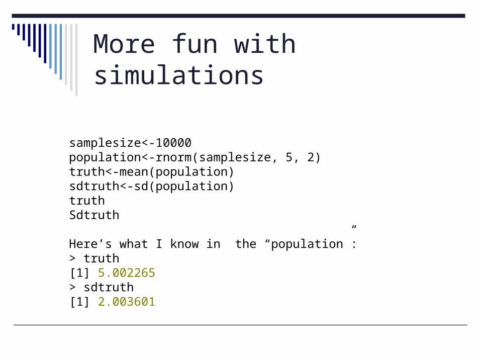
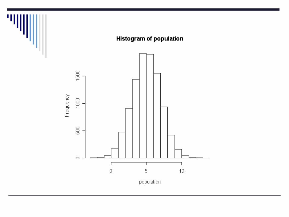
samplesize<-10000population<-rnorm(samplesize, 5, 2)truth<-mean(population)sdtruth<-sd(population)truthSdtruth

Here’s what I know in the “population”:> truth[1] 5.002265> sdtruth[1] 2.003601

More fun with simulations

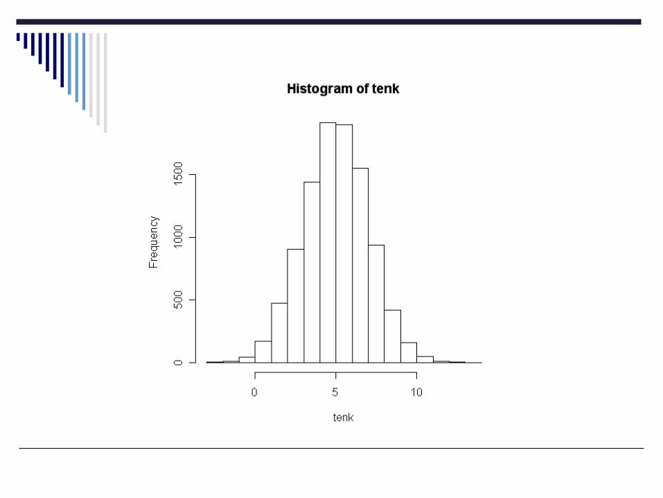
What do my samples look like?

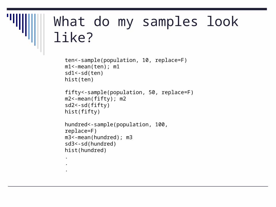
ten<-sample(population, 10, replace=F)m1<-mean(ten); m1sd1<-sd(ten)hist(ten)

fifty<-sample(population, 50, replace=F)m2<-mean(fifty); m2sd2<-sd(fifty)hist(fifty)

hundred<-sample(population, 100, replace=F)m3<-mean(hundred); m3sd3<-sd(hundred)hist(hundred)...

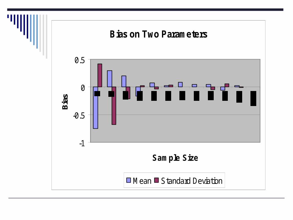
Bias on Two Parameters

-1

-0.5

0

0.5

Sample Size

Bia

s

Mean Standard Deviation

Sampling Sizes

In general, we’ve seen larger sample sizes yield more accurate conclusions.

Though the differences between very large and just “merely” large samples may in fact be negligible.

Requires us to turn to the concept of repeated sampling and sample variability.

Polls and Repeated Sampling

As individual researchers, you usually have one “shot” at it.

Statistical theory (classical) relies on the concept of long-run probability

Repeated trials …law of large numbers …central limit theorem

Maybe concepts you have heard of before? …or not.

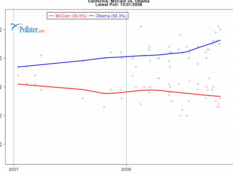
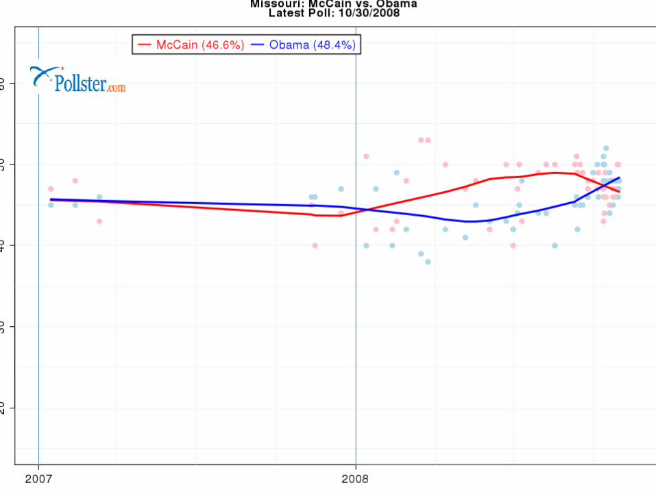
Side-trip to the 2008 Presidential Election Pollster.com allows us to think about

“repeated” sampling. This cite basis its analysis on all

available polls Why might this be a good thing? There is sampling variability in individual

samples. Let’s look at polls leading up to the Nov.

4th Election

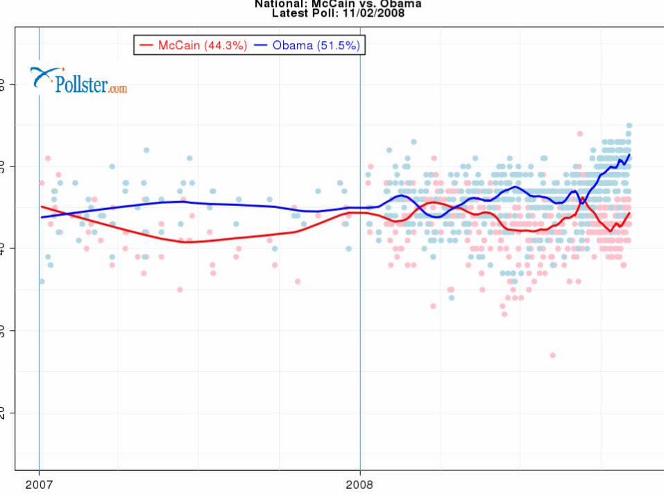
What are the “dots”

The blue dots are Obama percentage (estimates)

The red dots are McCain Why are they different? Variability in samples…sampling frames,

methodologies differ. Combine them, and you get a better

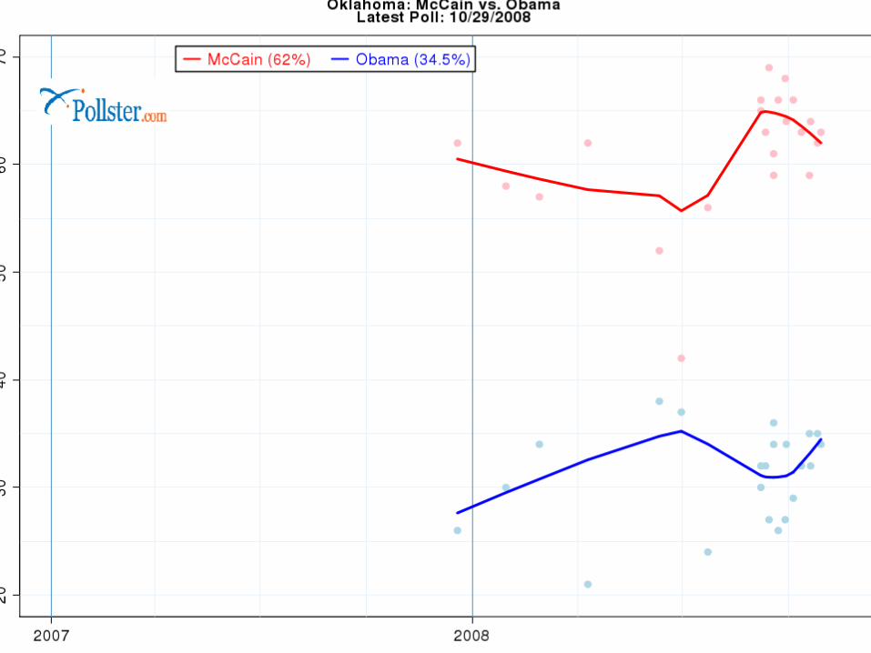
picture. Look at solid red and blue states.

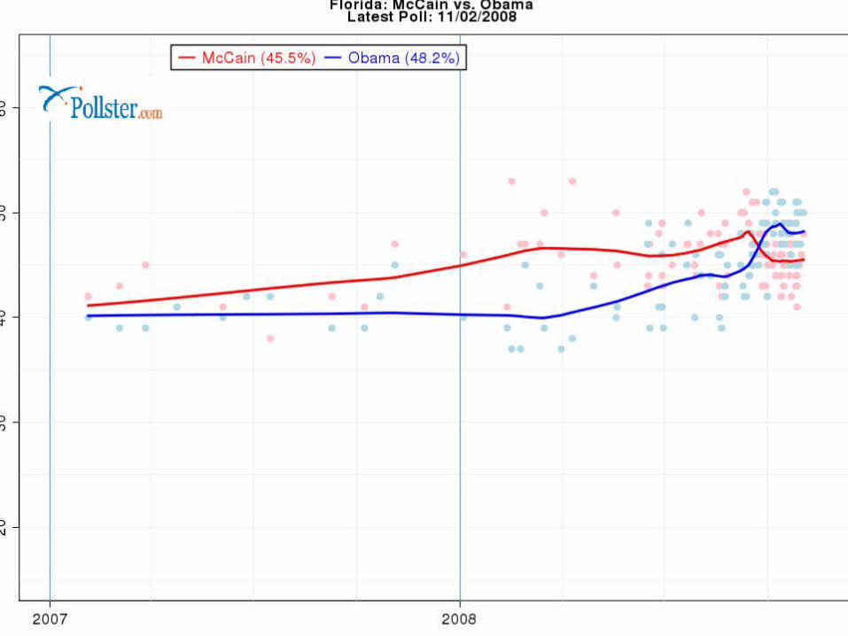
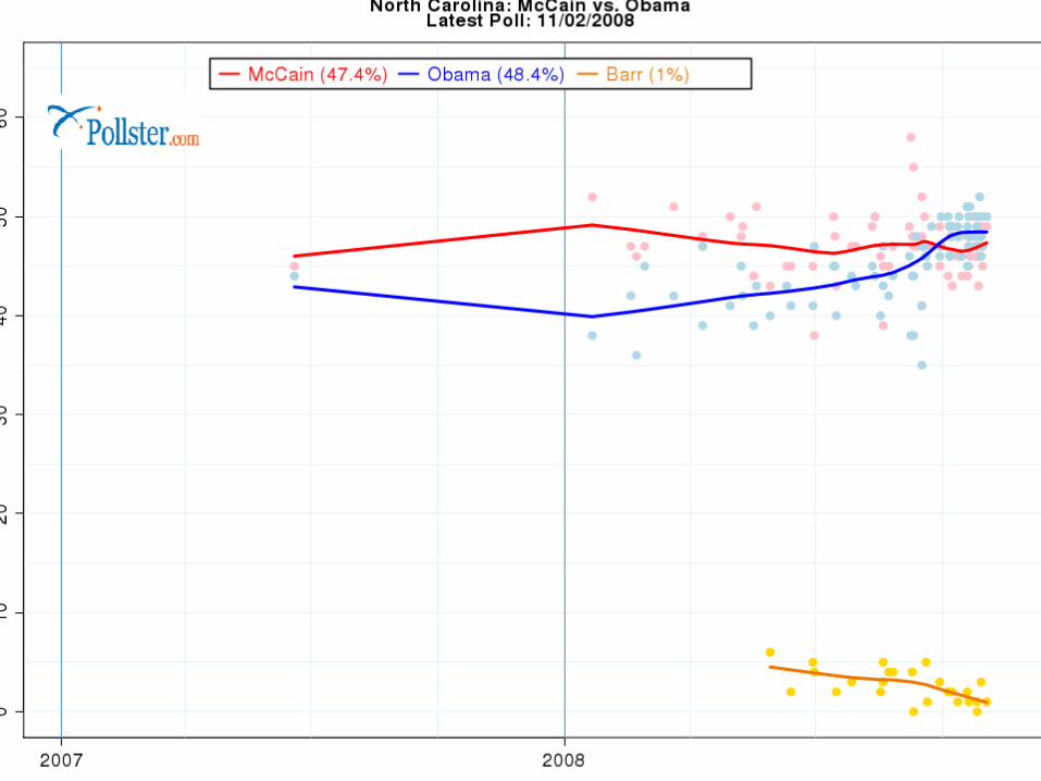
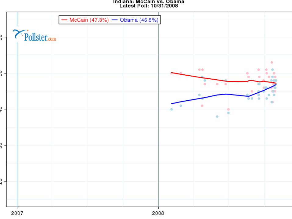
Polls

Note how the polls seem to be “clustering” as the election gets closer.

Why? Undecideds deciding? More certainty?

Let’s look at close states.

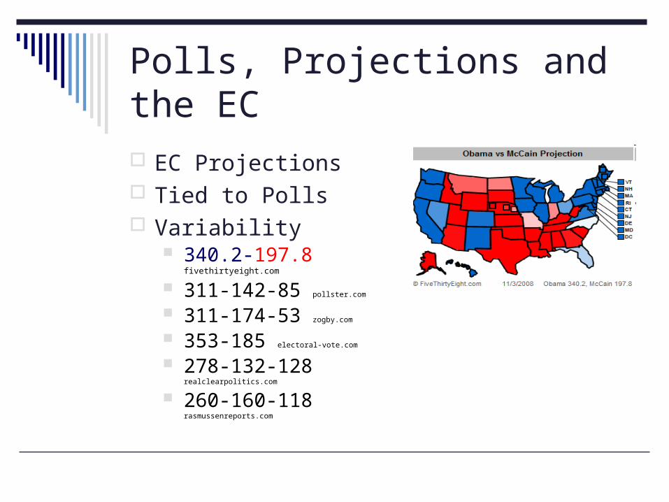
Polls, Projections and the EC

EC Projections Tied to Polls Variability

340.2-197.8 fivethirtyeight.com

311-142-85 pollster.com

311-174-53 zogby.com

353-185 electoral-vote.com

278-132-128 realclearpolitics.com

260-160-118 rasmussenreports.com

Understanding variability

We kind of see “repeated sampling” The basic idea:

The “truth” will be revealed if you just sample enough

But any one sample may be off in one direction or another.

Back to sampling Let’s simulate repeated sampling in R

More Simulation

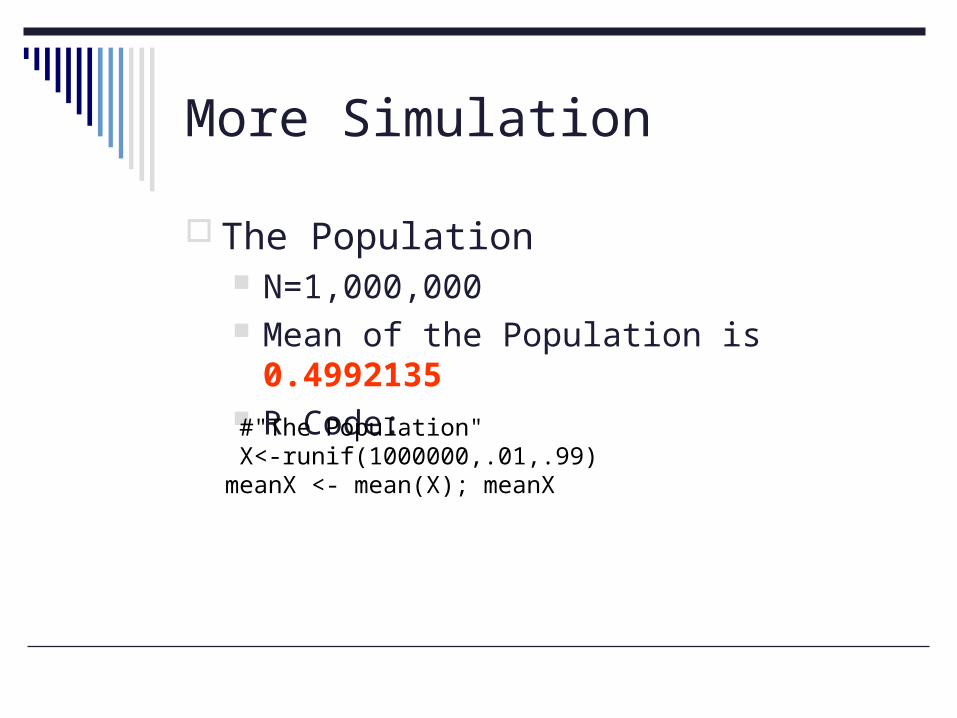
The Population N=1,000,000 Mean of the Population is 0.4992135 R Code:

#"The Population" X<-runif(1000000,.01,.99)meanX <- mean(X); meanX

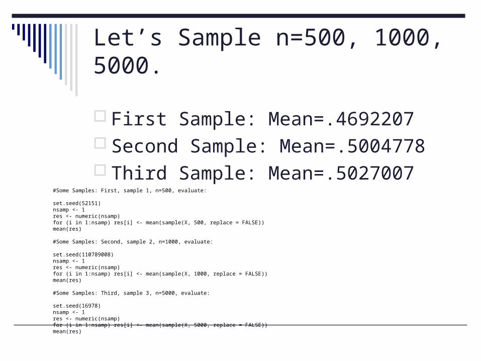
Let’s Sample n=500, 1000, 5000.

First Sample: Mean=.4692207 Second Sample: Mean=.5004778 Third Sample: Mean=.5027007

#Some Samples: First, sample 1, n=500, evaluate:

set.seed(52151)nsamp <- 1res <- numeric(nsamp)for (i in 1:nsamp) res[i] <- mean(sample(X, 500, replace = FALSE))mean(res)

#Some Samples: Second, sample 2, n=1000, evaluate:

set.seed(110789008)nsamp <- 1res <- numeric(nsamp)for (i in 1:nsamp) res[i] <- mean(sample(X, 1000, replace = FALSE))mean(res)

#Some Samples: Third, sample 3, n=5000, evaluate:

set.seed(16978)nsamp <- 1res <- numeric(nsamp)for (i in 1:nsamp) res[i] <- mean(sample(X, 5000, replace = FALSE))mean(res)

Repeated Sampling

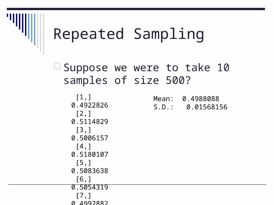
Suppose we were to take 10 samples of size 500?

[1,] 0.4922826 [2,] 0.5114829 [3,] 0.5006157 [4,] 0.5180107 [5,] 0.5083638 [6,] 0.5054319 [7,] 0.4992882 [8,] 0.4612303 [9,] 0.4897318[10,] 0.5016498

Mean: 0.4988088S.D.: 0.01568156

Lessons?

Sampling variability is a real issue. Range in estimates went from .46 to .52

Way under and way over estimate the mean in certain trials.

However, on average, “we’re close.” More simulations.

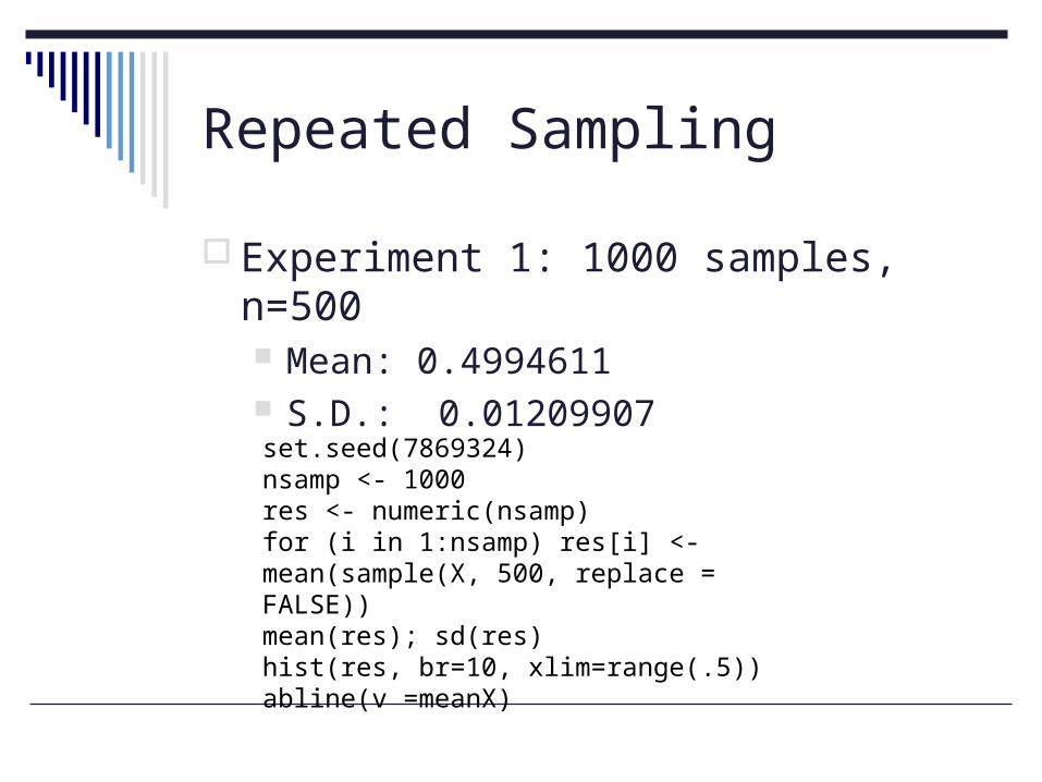
Repeated Sampling

Experiment 1: 1000 samples, n=500 Mean: 0.4994611 S.D.: 0.01209907

set.seed(7869324)nsamp <- 1000res <- numeric(nsamp)for (i in 1:nsamp) res[i] <- mean(sample(X, 500, replace = FALSE))mean(res); sd(res)hist(res, br=10, xlim=range(.5))abline(v =meanX)

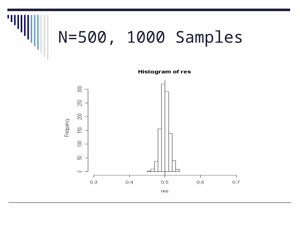
N=500, 1000 Samples

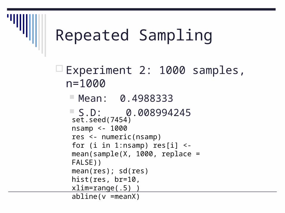
Repeated Sampling

Experiment 2: 1000 samples, n=1000 Mean: 0.4988333 S.D: 0.008994245

set.seed(7454)nsamp <- 1000res <- numeric(nsamp)for (i in 1:nsamp) res[i] <- mean(sample(X, 1000, replace = FALSE))mean(res); sd(res)hist(res, br=10, xlim=range(.5) )abline(v =meanX)

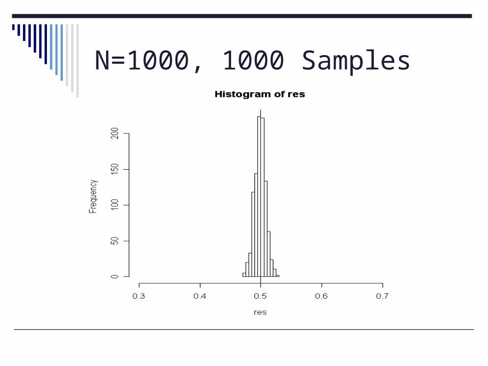
N=1000, 1000 Samples

Repeated Sampling

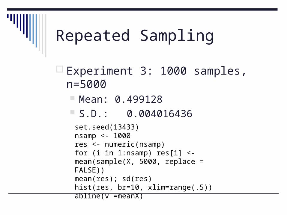
Experiment 3: 1000 samples, n=5000 Mean: 0.499128 S.D.: 0.004016436

set.seed(13433)nsamp <- 1000res <- numeric(nsamp)for (i in 1:nsamp) res[i] <- mean(sample(X, 5000, replace = FALSE))mean(res); sd(res)hist(res, br=10, xlim=range(.5))abline(v =meanX)

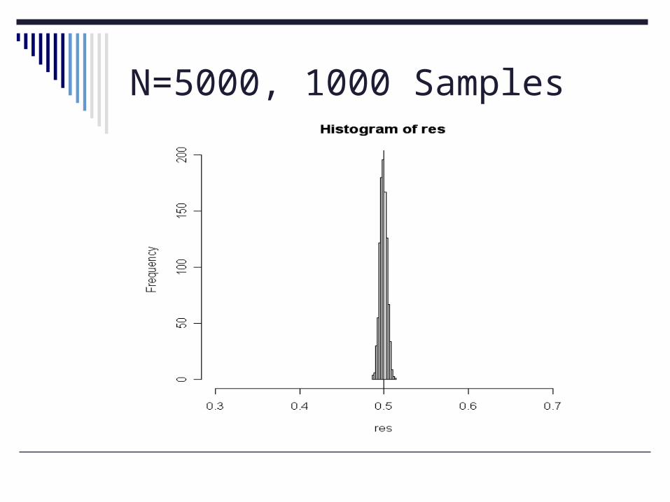
N=5000, 1000 Samples

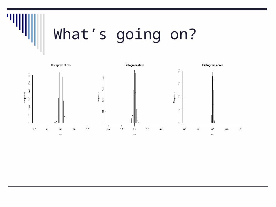
What’s going on?

Sampling Variability

If we “fix” the number of samples, what happened?

As n increases, variability decreases. “On average, our sample estimate is

“close” to the true value… AND, the variation across samples is

decreasing.

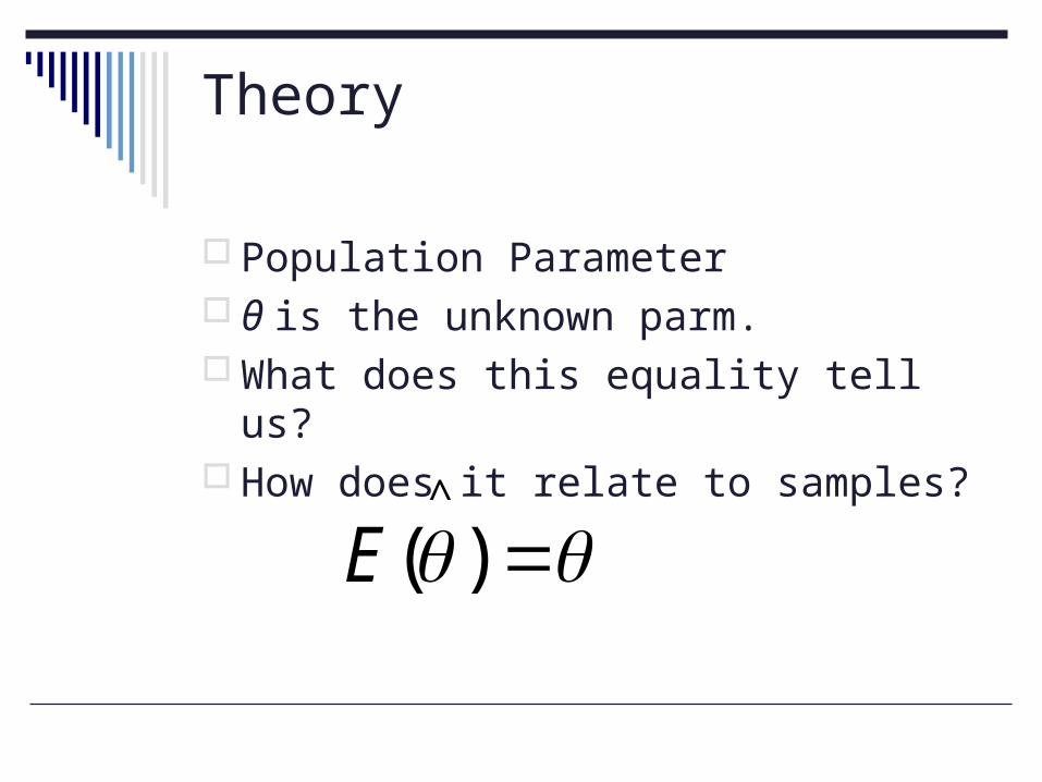
Theory

Population Parameter θ is the unknown parm. What does this equality tell us? How does it relate to samples?

)(^

E

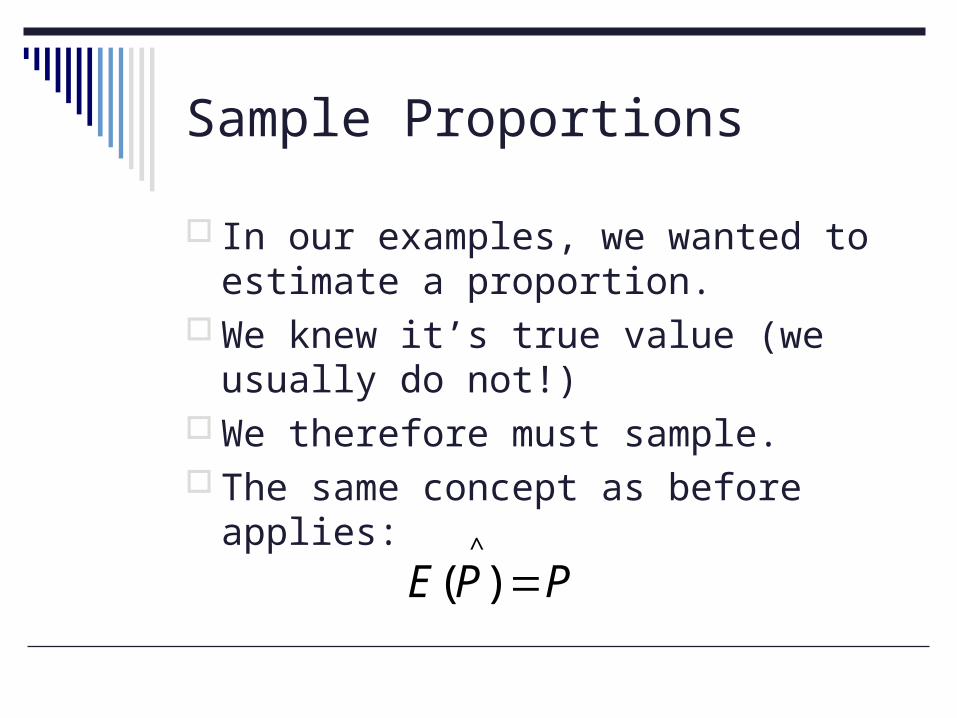
Sample Proportions

In our examples, we wanted to estimate a proportion.

We knew it’s true value (we usually do not!)

We therefore must sample. The same concept as before applies:

PPE ^

)(

Probability

“Over repeated samples, the expected value of the proportion will equal the true population proportion.”

This is a good thing. Sample estimates can do a good job of

approximating the population value. This permits generalizability.

Good sampling technique will produce “unbiased estimates.”

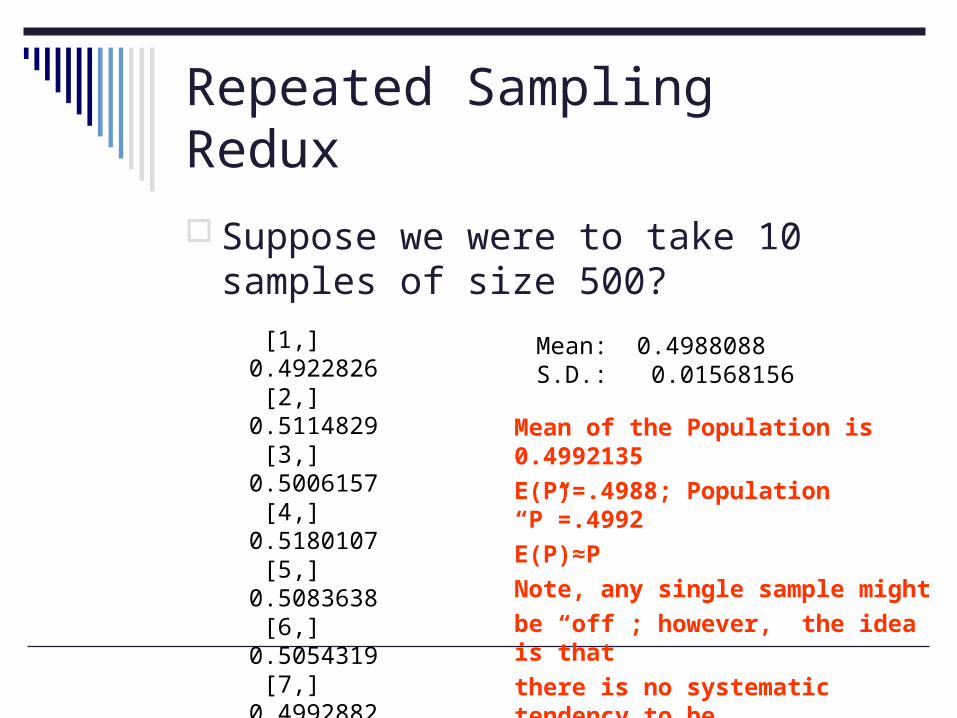
Repeated Sampling Redux

Suppose we were to take 10 samples of size 500?

[1,] 0.4922826 [2,] 0.5114829 [3,] 0.5006157 [4,] 0.5180107 [5,] 0.5083638 [6,] 0.5054319 [7,] 0.4992882 [8,] 0.4612303 [9,] 0.4897318[10,] 0.5016498

Mean: 0.4988088S.D.: 0.01568156

Mean of the Population is 0.4992135

E(P)=.4988; Population “P”=.4992

E(P)≈P

Note, any single sample might

be “off”; however, the idea is that

there is no systematic tendency to be

off one direction or the other.

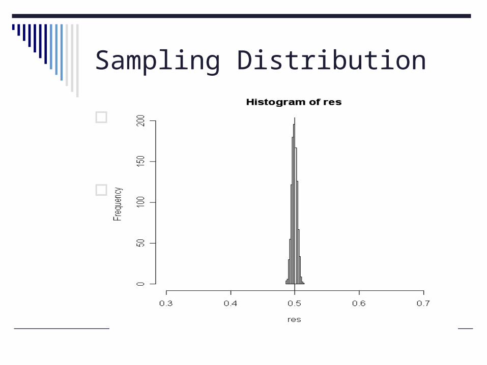
Sampling Distribution

What we’ve just gone through are simulations of SAMPLING DISTRIBUTONS

Defined: the distribution of a statistic that you obtain from repeated samples of size n from some population.

The Concept of Variance

How far might you be off in a particular sample?

Why, by the way, might you like to know this?

You usually only have ONE sample!! Is there a way we can determine this

degree of variability?

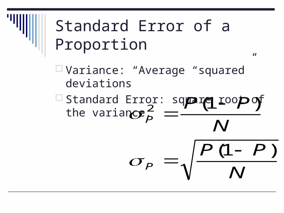
Standard Error of a Proportion

Variance: “Average “squared” deviations Standard Error: square root of the

variance.

N

PP

N

PP

P

P

)1(

)1(2

Standard Error in Action

Suppose the true population parameter is P. P=.50 In repeated samples, you would expect the

average sample statistic to approach .50 Recall prior simulation

What is the “sampling error”? Using formula from previous slide: [.5(1-.5)/100]1/2 =.05

Interpretation?

If the true population proportion is .50 and we took repeated (random) samples of size 100, the expected value of P would be .50 but the standard deviation would be .05.

.05 is our standard error of the sampling distribution. This is what ought to happen in repeated sampling.

More to it…that comes later.

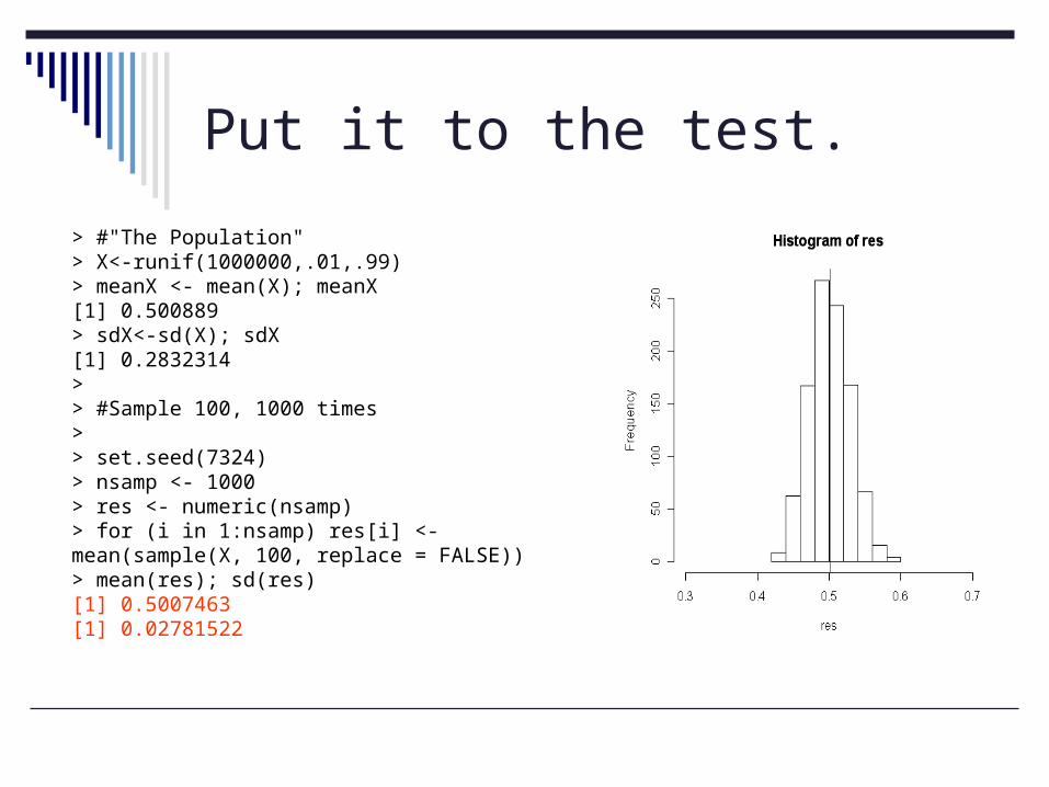
Put it to the test.

> #"The Population" > X<-runif(1000000,.01,.99)> meanX <- mean(X); meanX[1] 0.500889> sdX<-sd(X); sdX[1] 0.2832314> > #Sample 100, 1000 times> > set.seed(7324)> nsamp <- 1000> res <- numeric(nsamp)> for (i in 1:nsamp) res[i] <- mean(sample(X, 100, replace = FALSE))> mean(res); sd(res)[1] 0.5007463[1] 0.02781522

Result

What conclusions would I draw from my simulation?

“Best guess” of P is .50. The average deviation across samples is

about .03. My guess + my error allows me to

compute a CONFIDENCE INTERVAL Estimate +/- Error=C.I.

Confidence Interval

What I’ve really done in my simulation is computed a “68 percent confidence interval.”

.50 plus or minus .03 68 percent of all samples give a value for P

between (about) .47 and .53 Classical interpretation: In repeated samples of

size 100, the expected value of P will lie in the range .47 to .53, 68 percent of the time.

Why “68 percent”? 68-95-99.7 Rule and the Normal Distribution

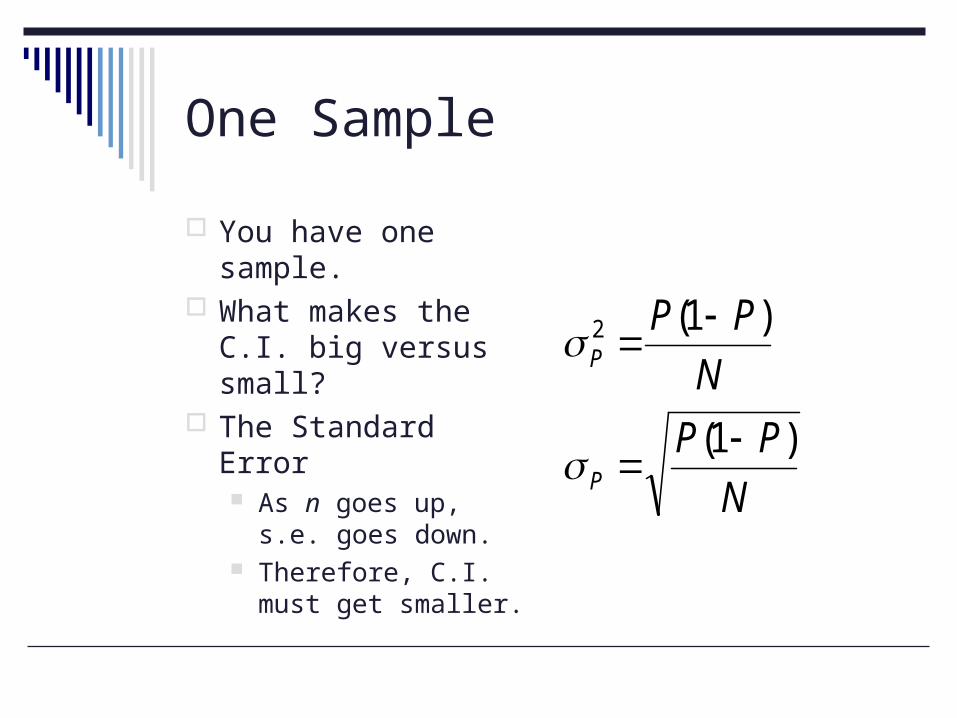
One Sample

You have one sample.

What makes the C.I. big versus small?

The Standard Error As n goes up, s.e.

goes down. Therefore, C.I. must

get smaller.

N

PP

N

PP

P

P

)1(

)1(2

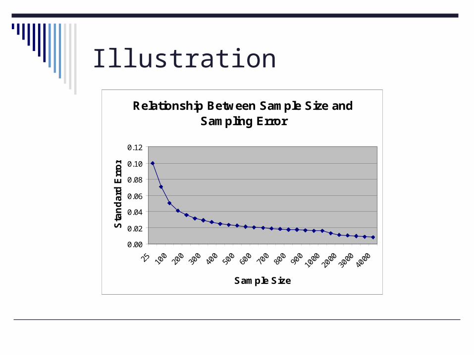
Illustration

Relationship Between Sample Size and Sampling Error

0.00

0.02

0.04

0.06

0.08

0.10

0.12

Sample Size

Sta

nd

ard

Err

or

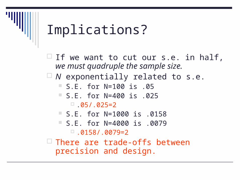
Implications?

If we want to cut our s.e. in half, we must quadruple the sample size.

N exponentially related to s.e. S.E. for N=100 is .05 S.E. for N=400 is .025

.05/.025=2 S.E. for N=1000 is .0158 S.E. for N=4000 is .0079

.0158/.0079=2 There are trade-offs between precision and

design.