The Sad Truth about Happiness Scales

Timothy N. Bond

Purdue University and IZA

Kevin Lang

Boston University, NBER, and IZA

We are grateful to Christopher Barrington-Leigh, Larry Katz, Jeff Liebman, Jens Ludwig, Andy Oswald,Daniel Sacks, Miguel Sarzosa, Justin Wolfers, and participants in seminars and sessions at the AmericanEconomic Association, Boston University, Indiana University-Purdue University Indianapolis, the FederalReserve Bank of New York, Georgetown University, McGill University, the University of Michigan and theUniversity of Waterloo, an informal brownbag lunch at Purdue University and the referees and editor fortheir helpful feedback and comments. We thank Brian Towell and Wanling Zou for their excellent researchassistance. The usual caveat applies, perhaps more strongly than in most cases.

1

Abstract

Happiness is reported in ordered intervals (e.g. very, pretty, not too happy). We review

and apply standard statistical results to determine when such data permit identification of

two groups’ relative average happiness. The necessary conditions for nonparametric identifi-

cation are strong and unlikely to be ever satisfied. Standard parametric approaches cannot

identify this ranking unless the variances are exactly equal. If not, ordered probit findings

can be reversed by lognormal transformations. For nine prominent happiness research areas,

conditions for nonparametric identification are rejected and standard parametric results are

reversed using plausible transformations. Tests for a common reporting function consistently

reject.

2

1 Introduction

A large literature has attempted to establish the determinants of happiness using ordered

response data from questions such as “Taking all things together, how would you say things

are these days – would you say that you are very happy, pretty happy, or not too happy?”1 We

review and synthesize how some well-known results from statistics and microeconomic theory

apply to such data, and reach the striking conclusion that the results from the literature are

essentially uninformative about how various factors affect average happiness.

The basic argument is as follows. There are a large (possibly infinite) number of states of

happiness which are strictly ranked. In order to calculate a group’s ‘mean’ happiness, these

states must be cardinalized, but there are an infinite number of arbitrary cardinalizations,

each producing a different set of means. The ranking of the means remains the same for

all cardinalizations only if the distribution of happiness states for one group first order

stochastically dominates that for the other. But, we do not observe the actual distribution

of states. We instead observe their distribution in a small number of discrete categories,

essentially a few intervals of their cumulative distribution functions.

Without additional assumptions we cannot rank the average happiness of two groups if

each has responses in the highest and lowest category. Using observed covariates to achieve

full nonparametric identification of the latent happiness distributions would require making

assumptions that happiness researchers generally claim to reject. We are therefore forced

to follow the standard approach and assume the latent distributions are from a common

unbounded location-scale family (e.g., an ordered probit). If we do, it is (almost) impossible

to get stochastic dominance, and the conclusion is therefore not robust to simple monotonic

transformations of the scale. In the case of the normal, there are always distributions in

the lognormal family that reverse the result. Even in the knife-edge case where it would

be possible to get stochastic dominance, the result would still be subject to the assumption

1Our analysis applies, mutatis mutandis, to other common questions such as those with five, seven or tenresponse categories

3

that all individuals report happiness the same way (a common reporting function), something

which we show empirically is unlikely to be the case.

We outline conditions under which we can identify the rank ordering of group happiness,

and then apply them to nine prominent results from the happiness literature. Not a single

one is satisfied in any case. We also describe a test for common reporting of happiness under

the assumption that happiness follows a distribution from the normal family. Whenever the

data allow us to perform such a test, we reject it.

2 Rank-Order Identification of Group Happiness

Suppose a researcher has two groups A and B, and she wishes to claim that members of

group A are, on average, happier than members of group B. What assumptions are required

to make such a claim?

Unfortunately, with happiness data we will never be able to simply compare the aver-

age group responses directly. That would require happiness to have been reported to the

researcher on an interval scale, the impossibility of which should be uncontroversial.2 Thus

we assume we are presented with an ordinal ranking of individuals’ happiness, and denote

individual i’s happiness in this order as Hi and the cdf of happiness for group k as Fk.3

Provided this ranking is complete, transitive, and continuous, from Debreu (1954) there

exists a cardinalization q such that, Hi > Hj ⇔ q (Hi) > q (Hj). Thus, in principle, we

can compare group means under this cardinalization. This approach is implicit in nearly

the entire empirical happiness literature. However, we know from Pareto (1909, pp. 541-2),

that q is not unique. There are infinite other cardinalizations, and changes in cardinaliza-

tion can change the ranking of means unless, as is well-known, there is first order stochastic

2It would require some way of eliciting each individual’s happiness on a scale where the difference betweena “99” and a “98” is the same difference in happiness as between a “97” and a “96”, or a “7” and a “6”, andso on. See Stevens (1946).

3To draw anything at all from the happiness literature, it is absolutely essential that it is possible to makeinterpersonal utility comparisons, an assumption we maintain throughout. But this is, itself, a controversialtopic. For a brief review, see Binmore (2009).

4

dominance (FOSD).4 Therefore, to conclude that group A is happier than group B, we must

observe that FA first order stochastically dominates FB.

In practice, happiness researchers never observe Fk directly. Instead they observe subjec-

tive responses in a small number of categories, such as “not too happy,” “pretty happy,” or

“very happy.” Suppose we have three categories S = {0, 1, 2}, and let rkS be the fraction of

respondents in group k who report happiness S. It is plausible that individuals follow a co-

herent introspective reporting rule, so that they report 0 if Hi ≤ H1i and 1 if H1

i ≤ Hi ≤ H2i .5

This will be uninformative about Fk if H1i and/or H2

i vary across individuals; a large number

of “very happy” responses in group A may indicate a high FA or low H2i s. For the moment

we assume H1i = H1, H2

i = H2∀i, that is a common reporting function, so the subjective

responses inform us of two points on each cdf: Fk(H1) = rk0 and Fk(H

2) = 1− rk2 .

Unfortunately, FA(H1) ≤ FB(H1) and FA(H2) ≤ FB(H2) (i.e., “stochastic dominance”

in the categories) does not directly imply FA FOSD FB. It simply narrows the set of possible

group distributions of happiness (see, for example, Manski 1988) to the set of all combinations

of cdfs for which FA(H1) = rA0 , FB(H1) = rB0 , FA(H2) = 1 − rA2 , FB(H2) = 1 − rB2 . In other

words, any two distributions that produce the observed happiness distribution in categories,

by group, describe the data equally well.

Following this, we say the rank order of A and B is identified only if for every pair

of distributions consistent with the data we have FA FOSD FB or FB FOSD FA.6 That

is, if A and B are rank order identified, the rankings of qA and qB will be the same for

any cardinalization of any distribution that can describe the data. Requiring rank-order

identification should again be uncontroversial. Rejecting this, requires making definitive

statements about rankings that hold for some arbitrary cardinalizations or equivalently some

arbitrary distributions, but not others satisfying the same a priori restrictions and describing

4See Lehmann (1955). This result entered the economics literature in the late 1960s (e.g, Hader andRussell 1969; Hanoch and Levy 1969).

5We will use a 3-point happiness scale going forward for illustrative purposes, but the discussion easilyextends to 4 or more categories.

6For a formal definition of rank order identification, see the Online Technical Appendix.

5

the data equally well.

We now explore the conditions under which group happiness is rank-order identified. We

begin with methods that do not rely on distributional assumptions, then consider restricting

the set of permissible distributions (i.e. parametric assumptions such as ordered probit).

2.1 Non-Parametric Identification

To simplify exposition, we normalize the cutoffs between the categories to H1 = 0 and

H2 = 1. Put differently, we restrict ourselves to the set of cardinalizations with this property.

When is the ranking of A over B identified without assuming a distribution for FA and

FB? If we use just the ordered responses, from Manski and Tamer (2002) we must have

rA0 = 0, rB2 = 0, and rA2 ≥ rB1 .7 If both groups have responses in the lowest category, the

data can be represented by distributions where nearly all the unhappy As are close to −∞

and all the unhappy Bs close to −ε, and vice versa. Similar logic applies when both groups

have responses in the highest category. Even if the lowest category for A and the highest

category for B are empty, all As might be clustered at the bottom of their categories (i.e., ε

and 1 + ε) while Bs might be clustered at their tops (i.e., −ε and 1 − ε); rA2 > rB1 ensures

that the distribution of A still dominates B in these situations. In practice, such a strong

set of conditions will never be satisfied (see Table 1 below) for a sample of any reasonable

size. Thus if happiness is reported using a discrete ordered scale, in practice we cannot

rank the mean happiness of two groups without additional information or restrictions on the

happiness distribution.

Now, suppose we have a vector of observable determinants of happiness X, and assume

we can partition i’s latent happiness

h∗i = ψ(Xi) + ui (1)

7If there are S + 1 categories, we require that rA0 = 0, rBS = 0 and Σs0r

Aj ≥ Σs−1

0 rBj ∀s = 1, ...S. We followthe literature on focusing on comparing means. Conditions for comparing, for example, medians are weakerand sometimes satisfied in practice.

6

into an observable component Xi with distribution FXk in group k, and an additively sep-

arable unobservable component ui with distribution F uk . The function ψ transforms the

observable components from their reported scale (e.g. dollars of income) to happiness under

the chosen cardinalization. Note that in addition to a common reporting function, we assume

ψ does not vary across groups. This assumption is implausible and also not strictly neces-

sary for identification, but we simplify the environment to achieve rank-order identification

as easily as possible.8

As Manski (1988) shows for a binary response, and Cameron and Heckman (1998) extend

to a general ordered response model, we can identify ψ, F u, and F h through assumptions

on the relations among X, u, and h, thereby avoiding assumptions about the distribution

of h or u.9 In our context, the key condition for nonparametric identification (Carneiro,

Hansen, and Heckman 2003, Cunha, Heckman, and Navarro 2007) is that the support of u

is contained in the support of ψ(X). As Manski discusses, this condition is critical;10 yet

it is problematic for happiness studies. The major observable determinants such as income

and marital status are bounded in practice, while factors such as physical and psychological

health are, at best, observed only in discrete ordered categories and at worst unobservable

and unbounded.11

To illustrate this problem, consider some authors’ claim that there is a “satiation point”

beyond which income does not increase happiness.12 If they are correct, then as X →

∞, ψ(X)→ ψ where X is income. Above −ψ we can identify the distribution of u based on

differences between reported happiness and that which would be predicted by ψ(X). But

8In order to place both groups on the same cardinalization, it is necessary that either both groups followthe same reporting rule, or both groups have some common X that has the same effect on the true latentvariable. See Urzua (2008).

9See the Online Technical Appendix for the full list of conditions.10See Manski’s (1988) discussion surrounding Proposition 2, Corollary 1.11While the condition is not formally testable, since we do not observe all possible draws of X from FX ,

we note that the individual with the lowest family income (as calculated by Stevenson and Wolfers 2009) inthe General Social Survey reports being “pretty happy.”

12Note that our appendix implicitly refutes such claims. Stevenson and Wolfers (2013) reviews a numberof papers which argue for a satiation point with respect to income, and find no support for this claim in anydataset using methods conventional within the happiness literature. Nonetheless, this has not stopped suchclaims from being made. See, for example, Jebb et al. (2018).

7

we cannot learn anything about the distribution of u below −ψ since all values in this range

result in a report of “not very happy” for any X. Within the set of admissible distributions,

u could be concentrated just below −ψ for one group and concentrated near −∞ for another.

Even if A stochastically dominates B above −ψ, the distributions could cross below −ψ, thus

we cannot have rank-order identification. A similar problem arises when X is bounded.

In sum, while theoretically possible, in practice we are unlikely to have the observables

necessary to non-parametrically identify the tails of the happiness distribution, without

which the means of two groups are never rank-order identified.

2.2 Parametric Identification

Absent nonparametric identification, we must either conclude that identification is impossible

or rely on parametric identification. Happiness researchers almost universally assume either

that the ordered responses are measured on a discrete interval scale, or that each group’s

latent happiness distribution is normal (i.e., ordered probit) or logistic (i.e., ordered logit).

These different approaches often yield similar results, leading some researchers to conclude

falsely that such assumptions are innocuous (e.g., Ferrer-i-Carbonell and Frijters 2004).13

Estimating ordered probit is equivalent to assuming the existence of a single cardinaliza-

tion under which both groups’ happiness is distributed normally, which is in and of itself very

strong.14 Further, the standard ordered probit happiness researchers use also assumes that

under this hypothesized cardinalization the variance of happiness is equal for all groups.15

The assumption is implausible and unnecessary for estimation, but necessary to obtain rank-

13This conclusion may be problematic even sidestepping the issues raised by this paper. Heckman andSinger (1984) show that despite three common distributional assumptions showing negative unemploymentduration dependence (and two strongly so), using an estimator that does not impose a parametric assumptionproduces the expected positive sign.

14Note that imposing that a single group’s happiness is distributed normally is simply selecting an arbitrarycardinalization.

15The normalization in many statistical packages (such as STATA) imposes that the variance of thenormally distributed unobservables is 1 and that the constant term is 0. If the ordered probit were appliedseparately without additional covariates, the program would report different cutpoints, implying a differentreporting function but the same mean and variance for all groups. In the online appendix, we normalize thefirst two cutpoints to 0 and 1 and estimate separate means and variances for each group.

8

order identification through ordered probit. It is well known that for unbounded distributions

from the location-scale family, one distribution is greater than the other in the sense of FOSD

if and only if their location parameters differ and their scale parameters are equal.16

Moreover, in practice, as the sample size gets large, we will never estimate identical scale

parameters even if the true scale parameters are equal.17 Of course, we may be unable to

reject equality, but we hardly need remind the reader that failure to reject and accepting the

null are not equivalent. Thus, for large sample sizes, these techniques will never be able to

identify which group is happier without further restrictions. Interestingly, this is true even

if the condition in section 2.1 is satisfied.

What types of cardinalizations reverse the conclusion drawn from the normal? Suppose

we estimate µA > µB, but σA < σB. The rank-ordering is preserved by all concave but not

all convex transformations (Hanoch and Levy 1969).18 One simple convex transformation

is ech∗, where c is a positive constant. As is well known, the resulting distribution is log

normal with mean

µτ = ecµ+.5c2σ2

(2)

which is increasing in σ. For c sufficiently large this transformation reverses the ranking.

When µA > µB and σA > σB, the ranking is preserved by convex transformations, but not

concave ones, such as −e−ch∗ . This generates a left-skewed lognormal distribution, with

mean

µτ = −e−cµ+.5c2σ2

(3)

which is decreasing in σ. Thus a sufficiently large c reverses the gap. These are both simple

monotonic transformations of the latent happiness variable. Since happiness is ordinal, these

16The proof of this is a simple algebra exercise dating at least to Bawa (1975). A close corollary serves asan exercise in a popular graduate textbook (Casella and Berger 2002, p. 407). An alternative proof for themultivariate normal is in Muller (2001).

17Assuming estimation by maximum likelihood, the estimates will be asymptotically normal and theirdifference will also have a normal limiting distribution. See the working paper for more discussion.

18Hanoch and Levy show this result for any distribution which can be characterized by two parametersthat are independent functions of the mean and variance of the distribution, a subset of the location-scalefamily.

9

transformations represent the responses equally well. It is possible to achieve stochastic

dominance using bounded distributions from the location-scale family, such as the uniform.

But, there is little or no reason to prefer a bounded distribution over unbounded ones, from

the location-scale family or otherwise, that do not exhibit FOSD.

In sum, it is impossible to rank order groups using only the parametric assumptions

made in the literature or any of the location/scale distributions typically used by empirical

researchers. Identification might be achieved by applying additional restrictions to a standard

distribution (i.e. placing restrictions on the set of permissable cardinalizations). Addressing

whether a researcher could make a compelling case for such restrictions or the profession could

reach a consensus on them would take us into the philosophy and sociology of science and

beyond the scope of this paper. In the empirical section below we show that standard results

can almost always be reversed using what we are confident are plausible transformations

within the lognormal.

2.3 Reporting Function

It follows from our discussion that if true happiness is normally distributed with different

variances between groups, there is always a reporting function such that the difference in

mean reported happiness has the opposite sign from the true difference. But even this result

assumes that all individuals report their happiness the same way. Up to now, it has been

convenient to assume a common reporting function, but as we show in the empirical section,

this assumption is unlikely to be correct.19

King et al. (2004) propose circumventing differences in reporting functions by using

‘vignettes’ to anchor the scale on which people report happiness. This requires that (1)

individuals evaluate the vignettes on the same scale as they evaluate their own well-being

(“response consistency”), and (2) each individual perceives the same value from the vignettes

19See also Ravallion, Himelein, and Beegle (2016), who find evidence of substantial differences in thereporting function (“scale heterogeneity” in their terminology) for subjective poverty status both within andacross countries.

10

(“vignette equivalence”). Both assumptions are strong, the second particularly so, given het-

erogenous preferences. Moreover, as discussed above, even if we could place all individuals’

happiness on a common scale, monotonic transformations of this scale would reverse group

rankings.

Still, it is often easy to test for a common reporting function under a given parametric

assumption. Suppose, for example, happiness is reported in N ≥ 4 categories, and we impose

normality, setting the first two cutoffs to be 0 and 1. This ‘identifies’ the means and variances

of the distributions and leaves N − 3 cutoffs free. It is straightforward to test whether the

free cutoffs are the same for all groups. Of course, faced with a rejection, the researcher

is free to conclude either that her initial conjecture about the cardinalization was wrong or

that the reporting functions differ, but we believe that, at the very least, testing the joint

hypothesis should be standard procedure.20

3 Empirical Tests of the Happiness Literature

In the previous section we outlined the conditions under which the rank order of happiness for

groups can be identified using categorical data on subjective well-being. We now put these

into practice for nine key results from the happiness literature: the Easterlin (1973, 1974)

Paradox for the United States, whether happiness is U-shaped in age, the optimal policy

trade-off between inflation and unemployment, rankings of countries by happiness, whether

the Moving to Opportunity program increased happiness, whether marriage increases hap-

piness, whether children decrease happiness, the relative decline of female happiness in the

United States, and whether disabilities decrease happiness.21 For each of these, we first

ask if we can draw any conclusions without assuming a parametric distribution by applying

the criterion in section 2.1. We then test whether we can reject equal variances under an

20Note that we can also reject for any cardinalization in which the latent variable and cutpoints can berepresented by the same monotonic transformation of the normal.

21For details of the estimation procedures and literature review of these results, see the Online EmpiricalAppendix.

11

assumed normal distribution, and determine whether the conclusions can be reversed using

a left-skewed or right-skewed lognormal transformation, as outlined in section 2.2, and the

degree of skewness required. Finally, when we have sufficient happiness categories, we also

test for equal reporting functions assuming the existence of a cardinalization from the normal

family as discussed in section 2.3.

Table 1 summarizes the results. None of these results are identified non-parametrically.

Moreover, in the eight cases for which we can test for equality of variances under a parametric

normal assumption, we reject equality. Thus we never have rank order identification, and

can always reverse the standard conclusion by instead assuming a left-skewed or right-skewed

lognormal. Further, in the seven cases where we are able to test for stability of the reporting

function, we reject every time.

Thus if researchers wanted to draw any conclusions from these data, they would have

to eschew rank order identification. In other words, they would have to argue that it is

appropriate to inform policy based on one arbitrary cardinalization of happiness but not

another, or equivalently that some cardinalizations are “less arbitrary” than others. It is

unclear from where such an argument would come, or why we should apply a different

standard for happiness research than other branches of economics.

Even if someone were to make this case, we cannot see how such a standard would say

that distributions that resemble objective economic variables would be implausible. In the

Online Empirical Appendix we further show that nearly every result can be reversed by a

lognormal transformation that is no more skewed than the wealth distribution of the United

States.22 Even within this class of distributional assumptions, we cannot draw conclusions

stronger than “Nigeria is somewhere between the happiest and least happy country in the

world,” or “the effect of the unemployment rate on average happiness is somewhere between

very positive and very negative.” To be clear, we are not proposing that satisfying this

minimal criterion would make a result convincingly robust. It is plausible that happiness

22The exceptions are that the disabled are less happy than the non-disabled and that married women arehappier than unmarried women. In both cases, we reject a common reporting function.

12

is more skewed than wealth is. And it is certainly not self-evident that happiness must be

normal or lognormal. Happiness could be left-skewed for men and right-skewed for women,

and their distributions might come from different families. And any claims of robustness

would have to address our consistent finding of different reporting functions across groups.

While we cannot rule out the possibility that happiness researchers will be able to find

cardinalizations that are both consistent with a common reporting function and are robust

within some parametric restrictions that most economists will find compelling, we are not

sanguine about this prospect.

4 Conclusion

It is essentially impossible to rank two groups based on their mean happiness using the types

of survey questions prevalent in the literature. Because happiness is ordinal, two groups can

be ranked only if the distribution of one group first order stochastically dominates the dis-

tribution of the other. We can infer FOSD from the ordered response data alone only in

extreme cases that do not occur in practice. The conditions for full identification through

variation in observables are also violated. The parametric assumptions in the literature are

incapable of producing FOSD without untenably strong assumptions about the happiness

distribution. All of these conclusions are direct implications of well-established and uncon-

troversial results.

What then can we learn from such data? The regression estimates from ordered probit or

logit are only accurate for one particular, arbitrary (and possibly nonexistent) cardinalization

of happiness. This does not discount the actual self-reports, themselves. If we are only

concerned about the number of people who subjectively consider their emotional state “not

too happy,” we can estimate effects using conventional binary response models. But, it is

important to recognize that such an interpretation is much narrower than proponents of

the use of average happiness measures currently claim for them. Subjective perceptions are

13

subjective and introspective, and generalizations drawn from such analysis are particularly

sensitive to differences in the reporting function.

Researchers who wish to continue to interpret such questions more broadly need to be

explicit about the assumptions underlying their conclusions, and justify their particular

cardinalization or parametric assumption relative to other plausible alternatives. It is not

clear what this justification could be, and our empirical work finds little evidence that even

very strong restrictions will yield interpretable results. At a bare minimum, we would require

a functional form assumption that survived the joint test of the parametric functional form

and common reporting function across groups. Certainly calls to replace GDP with measures

of national happiness are premature.

14

References

Bawa, Vijay S. 1975. “Optimal Rules for Ordering Uncertain Prospects.” Journal of Finan-

cial Economics 2 (1): 95-121.

Binmore, Ken. 2009. “Interpersonal Comparison of Utility” In The Oxford Handbook of

Philosophy of Economics, edited by Harold Kincaid and Don Ross, 540-59. New

York: Oxford University Press.

Cameron, Stephen V., and James J. Heckman. 1998. “Life Cycle Schooling and Dynamic

Selection Bias: Models and Evidence for Five Cohorts of American Males.” Journal

of Political Economy 106 (2): 262-333.

Carneiro, Pedro, Karsten T. Hansen, and James J. Heckman. 2003. “Estimating Distri-

butions of Treatment Effects with an Application to the Returns to Schooling and

Measurement of the Effects of Uncertainty on College Choice.” International Eco-

nomic Review 44 (2): 361-421.

Casella, George, and Roger L. Berger. 2002. Statistical Inference. Pacific Grove, CA:

Duxbury.

Cunha, Flavio, James J. Heckman, and Salvador Navarro. 2007. “The Identification and

Economic Content of Ordered Choice Models with Stochastic Thresholds.” Interna-

tional Economic Review 48 (4): 1273-309.

Debreu, Gerard. 1954. “Representation of a Preference Ordering by a Numerical Function.”

in Decision Processes, edited by R.M Thrall, C.H. Coombs, and R.L Davis, 159-64.

Oxford, England: John Wiley & Sons.

Easterlin, Richard A. 1973. “Does Money Buy Happiness?” The Public Interest 30 (Winter):

3-10.

Easterlin, Richard A. 1974. “Does Economic Growth Improve the Human Lot?” In Nations

and Households in Economic Growth: Essays in Honor of Moses Abramovitz, edited

by Paul A. David and Melvin W. Reder, 89-125. New York: Academic Press.

Ferrer-i-Carbonell, Ada, and Paul Frijters. 2004. “How Important is Methodology for the

15

Estimates of the Determinants of Happiness.” Economic Journal 114 (497): 641-59.

Hader, Joseph, and William R. Russell. 1969. “Rules for Ordering Uncertain Prospects.”

American Economic Review 59 (10): 25-34.

Hanoch, G. and H. Levy. 1969. “Efficiency Analysis of Choices Involving Risk.” Review of

Economic Studies 36 (3): 335-46.

Heckman, James J., and Burton Singer. 1984. “A Method for Minimizing the Impact of

Distributional Assumptions in Econometric Models for Duration Data.” Econometrica

52 (2): 271-320.

Jebb, Andrew T., Louis Tay, Ed Diener, and Shigehiro Oishi. 2018. “Happiness, Income

Satiation, and Turning Points around the World.” Nature Human Behavior 2: 33-8.

King, Gary, Christopher J. L. Murray, Joshua A. Salomon, and Ajay Tandon. 2004. “En-

hancing the Validity and Cross-Cultural Comparability of Measurement in Survey

Research.” American Political Science Review 98 (1): 191-207.

Lehmann, E. L. 1955. “Ordered Families of Distributions.” Annals of Mathematical Statistics

26 (3): 399-419.

Manski, Charles F. 1988. “Identification of Binary Response Models.” Journal of the Amer-

ican Statistical Association 83 (403): 729-38.

Manski, Charles F., and Elie Tamer. 2002. “Inference on Regressions with Interval Data on

a Regressor or Outcome.” Econometrica 70 (2): 519-46.

Muller, Alfred. 2001. “Stochastic Ordering of Multivariate Normal Distributions.” Annals

of the Institute of Statistical Mathematics 53 (3): 567–75.

Pareto, Vilfredo. 1909. Manuel d’economie politique. Translated by Alfred Bonnet. (Paris:

V. Giard et E. Briere).

Ravallion, Martin, Kristen Himelein, and Kathleen Beegle. 2016. “Can Subjective Ques-

tions on Economic Welfare be Trusted? Evidence for Three Developing Countries.”

Economic Development and Cultural Change 64 (4): 697-726.

Stevens, S.S. 1946. “On the Theory of Scales and Measurement.” Science 103 (2684): 677-80.

16

Stevenson, Betsey and Justin Wolfers. 2009. “The Paradox of Declining Female Happiness.”

American Economic Journal: Economic Policy 1 (2): 190-225.

Stevenson, Betsey and Justin Wolfers. 2013. “Subjective Well-Being and Income: Is there

any Evidence of Satiation?” American Economic Review 103 (3): 598-604.

Urzua, Sergio. 2008. “Racial Labor Market Gaps: The Role of Abilities and Schooling

Choices.” Journal of Human Resources 43 (4): 919-74.

17

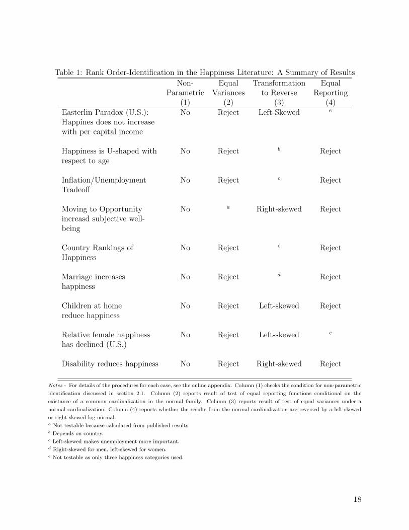
Table 1: Rank Order-Identification in the Happiness Literature: A Summary of Results

Non- Equal Transformation EqualParametric Variances to Reverse Reporting

(1) (2) (3) (4)Easterlin Paradox (U.S.): No Reject Left-Skewed e

Happines does not increasewith per capital income

Happiness is U-shaped with No Reject b Rejectrespect to age

Inflation/Unemployment No Reject c RejectTradeoff

Moving to Opportunity No a Right-skewed Rejectincreasd subjective well-being

Country Rankings of No Reject c RejectHappiness

Marriage increases No Reject d Rejecthappiness

Children at home No Reject Left-skewed Rejectreduce happiness

Relative female happiness No Reject Left-skewed e

has declined (U.S.)

Disability reduces happiness No Reject Right-skewed Reject

Notes - For details of the procedures for each case, see the online appendix. Column (1) checks the condition for non-parametric

identification discussed in section 2.1. Column (2) reports result of test of equal reporting functions conditional on the

existance of a common cardinalization in the normal family. Column (3) reports result of test of equal variances under a

normal cardinalization. Column (4) reports whether the results from the normal cardinalization are reversed by a left-skewed

or right-skewed log normal.a Not testable because calculated from published results.b Depends on country.c Left-skewed makes unemployment more important.d Right-skewed for men, left-skewed for women.e Not testable as only three happiness categories used.

18

A Online Empirical Appendix

In this appendix, for several of the most prominent research areas in the happiness

literature, we test empirically the conditions for rank order identi�cation described

in the main text. As discussed there, and our results below con�rm, the conditions

under which the ranking of the mean happiness of two groups is nonparametrically

identi�ed are unlikely to be satis�ed in practice. Therefore we are forced to rely on

parametric identi�cation.

The most common parametric assumption is that there exists a cardinalization

under which the happiness of each of two groups is distributed normally. If we assume

normality and the two groups have di¤erent means and variances, then if group A

has a higher mean than group B, there also exists a cardinalization of happiness

using the family of log-normal distributions under which group B has a higher mean

than group A. We provide tests for, and reject, equal variances for each of the cases

we consider.

We then explore empirically the types of cardinalizations that are required to

reverse the major results in the happiness literature. While it is impossible for any

single result to be irreversible, some results require more dramatic deviations from

normality than others. Additionally, some results are only reversible by skewing the

distribution to the left, while others are only reversible by skewing the distribution to

the right. Our exercises indicate that the set of results one can claim from the happi-

ness literature is highly dependent on one�s beliefs about the underlying distribution

of happiness in society, or the social welfare function one chooses to adopt.

A-1

Any conclusions reached from these parametric approaches rely on the assumption

that all individuals report their happiness in the same way. When the data permit,

we test for equal reporting functions, conditional on the existence of a common

cardinalization from the normal family. We reject this assumption in all cases in

which we test it.

This appendix is organized as follows. In section A.1, we discuss the methods

we will use to implement our assessment. Section A.2 reviews our data sources.

Our main results lie in section A.3, where we test for rank-order identi�cation and

determine the cardinalizations (within the log-normal family) that reverse nine key

results from the happiness literature: the Easterlin Paradox, the �U-shaped�relation

between happiness and age, the happiness trade-o¤ between in�ation and unemploy-

ment, cross-country comparisons of happiness, the impact of the Moving to Oppor-

tunity program on happiness, the impact of marriage and children on happiness, the

�paradox�of declining female happiness, and the e¤ect of disability on happiness.

Section A.4 concludes.

A.1 Methods

A.1.1 Distribution-Free Comparisons

We begin each case by asking if it is possible to say anything about the groups

being studied without assuming happiness can be cardinalized along some parametric

probability distribution. Consider two groups A and B who report their happiness in

three categories, where ri0; ri1; and r

i2 are the fraction of responses in each category for

group i. As we discuss in the main text, in the absence of a distributional assumption,

A-2

the ranking of A over B is identi�ed only if rA0 = 0; rB2 = 0; and r

A2 � rB1 . We thus

look at the distribution of responses to the happiness question across each of the

groups being studied, and see if any two pairs of groups satisfy this condition. In no

case is this condition satis�ed.

A.1.2 Normal Cardinalization

We then ask if we can make comparisons across groups assuming there exists a

cardinalization of happiness under which the distribution would be normal within

each group. As discussed in the main text, provided that the standard deviation

of happiness does not vary across groups, the ranking of the means provided by

the normal cardinalization would hold for any alternative cardinalization. In other

words, the rankings are identi�ed by this parametric assumption.

When happiness is recorded on a three-point scale, it is straightforward to calcu-

late the means and variances under normality as the model is just identi�ed. How-

ever, in some of our applications we will be interested in estimating the distribution

of happiness net of factors such as income or employment status that vary across

groups. To do this, we estimate a heteroskedastic probit model using the oglm com-

mand in STATA created by Williams (2010). Denote S 2 f0; 1; 2g as an individual�s

answer to a 3-point subjective well-being survey. The model assumes that S is de-

A-3

termined by a latent variable h�,

S = 0 if h� < k0

S = 1 if k0 � h� � k1 (1)

S = 2 if k1 < h�

and that

h�i = �mDi + �mXi + "i (2)

where k0 and k1 are cut-o¤ values of the latent variable that determine the observed

response, Di is an indicator for the group we are studying, Xi is a vector of individual

speci�c controls and "i is a normally distributed error term with mean 0 and variance

�i with

�i = �� exp(�sDi + �sXi) (3)

In other words, the model varies from the classic ordered probit in that it allows the

observable characteristics to in�uence the variance of the error term in the latent

variable.

Just as with a textbook ordered probit, one cannot separately identify the cut

points from the variance. The oglm routine normalizes �� = 1 and estimates �s; �s;

am � (�m=��); and bm � (�m=��). It easy to transform the oglm estimates into

their equivalents under our preferred normalization, where k0 = 0 and k1 = 1. The

A-4

estimated mean and variance for our control group Di = 0 will be

�0 = �k0(�o) (4)

�0 =1

k1 � k0(5)

and for Di = 1;

�1 = �0am + �0 (6)

�1 = �0 exp(as) (7)

These produce estimates for the mean and variance of the distribution only at a

speci�c set of values for controls, namely X = 0. When applicable, we de-mean

the controls, so our estimates can be thought of as characterizing the distribution of

happiness for individuals who di¤er in their group membership, but otherwise pos-

sess the mean characteristics throughout the entire population (regardless of group

membership). This method extends easily to more groups.

Having estimates of the standard deviation across groups, we then perform a joint

test of equality. Provided we reject that test, alternative cardinalizations will reverse

the ordering of means provided by the normal. However we strongly emphasize that

a failure to reject this test does not mean that the ranking is identi�ed. Rank order

identi�cation through the normal assumption requires the standard deviations across

groups are exactly equal, a hypothesis that we may fail to reject but can, of course,

never accept.

A-5

A.1.3 Applying Other Cardinalizations

Once we have estimated � and � under the normality assumption, we can re-

cardinalize happiness. We limit attention to cardinalizations that transform the

distribution from normal to left-skewed and right-skewed log-normal distributions.

Recall from the main text that for a given constant c, the mean of happiness once

re-cardinalized to a right-skewed log-normal distribution will be

�� = exp(c�+1

2c2�2); (8)

while for a left-skewed log-normal

�� = � exp(�c�+ 12c2�2): (9)

As the transformed mean of the right-skewed log-normal distribution is increasing in

the variance of the normal cardinalization, and the mean of left-skewed log-normal

distribution is decreasing in the variance of the normal cardinalization, so long as

�21 6= �22, there will always be a c such that one of these transformations reverses the

original ordering of two groups, where

c =

����2(�1 � �2)

�22 � �21

���� : (10)

A negative term within the absolute value indicates a left-skewed log normal is re-

quired.

We will explore how adopting various left-skewed and right-skewed log-normal

A-6

transformations a¤ects the conclusions one would draw from data and, when ap-

plicable, what c is required to reverse the result. Because of the nature of the

transformations, increasing c increases the skewness of the resulting distribution. To

provide some context to the amount of skewness our transformations imply, we will

provide comparisons to the skewness of the income and wealth distributions of the

United States, where the means are at the 74th and 80th percentiles, respectively

(Diaz-Gimenez, Glover, and Rios-Rull, 2011).1 These are reference points for the

reader, not a guideline. If a researcher were willing to ignore our warnings and try

to draw inference from assumed distributions, knowing full well that the results are

identi�ed only through functional form assumptions and only for a subset of car-

dinalizations implied by these assumptions, we believe it would still be exceedingly

di¢ cult to argue that results from other distributional assumptions that resemble

real-life distributions of economic variables are not just as valid. The converse is

certainly not true. Moreover, by limiting ourselves to log-normal transformations,

we are not determining the minimum amount of skewness necessary to overturn any

result. Instead we ask how extreme a transformation from a very restrictive class of

distributions is required to reverse the result.

A.1.4 Reporting Function

The analysis thus far has rested on the assumption that individuals from di¤erent

groups report their happiness in the same way. With a 3-point scale, such as the

1The percentile position of the mean for the lognormal distribution of transformation c is 12 +

12 erf(

c�2p2). This implies that the transformation that would generate equivalent skewness to the

income distribution (as measured by the percentile ranking of the mean) is c = 1:29� , and c = 1:68

�for the wealth distribution.

A-7

popular GSS question, we do not have su¢ cient degrees of freedom to identify dif-

ferences in reporting separately from di¤erences in the latent variable.2 In other

words, such data cannot distinguish between men being happier than women and

men having lower standards for reporting their happiness.

Adding a fourth categorical response, as is the case in the Eurobarometer Trend

File and World Values Survey data we will use below, grants us the freedom to

test this hypothesis, conditional on the true distribution being in the normal family

(including members of the lognormal family), using a likelihood ratio test. Our

unconstrained model estimates ordered probits separately for each group. The �rst

two cut-points are normalized to 0 and 1, while the mean, variance, and highest cut-

points are estimated from data. Our constrained model is a heteroskedastic ordered

probit that allows for group-speci�c means and variances, but forces the highest cut-

point to be identical. This generates a �2-statistic with degrees of freedom equal to

the number of happiness categories above three, multiplied by the number of groups

minus one.

A.2 Data

We use and describe here data common in the happiness literature.

2We have referred throughout this article to the way in which an individual transforms subjectivefeelings into a numerical value or category reported on a survey as the �reporting function,�and thatif two individuals transform their feelings into numerical values di¤erently they lack a �commonreporting function.� This follows the language used by Oswald (2008). The problem has beenalternatively referred to as �di¤erential item functioning�by King et. al (2004), �scale recalibration�by Adler (2013), and �heterogeneous standards�by Fleurbaey and Blanchet (2013).

A-8

A.2.1 General Social Survey

The General Social Survey (GSS) is the most widely used data to study happiness in

the United States. It has surveyed a nationally representative sample of Americans

on a variety of social attitudes annually or biennially since 1972. It asks, �Taken

all together, how would you say things are these days �would you say that you

are very happy, pretty happy, or not too happy?� This language and its 3-point

scale has been commonly adopted by other studies, including the assessments of

the Moving to Opportunity project (MTO) which we discuss in the next section.

While the question remains constant over time, its position in the survey does not,

which could lead to biases in responses in di¤erent years.3 We therefore use the

publicly available replication �le provided by Stevenson and Wolfers (2009), who use

split-ballot experiments to modify the data to account for these di¤erences.4

A.2.2 Eurobarometer Trend File

The Mannheim Eurobarometer Trend File 1970-2002 combines and harmonizes sev-

eral di¤erent annual surveys of the European Community, thus enabling within-

and cross-country comparisons over time. The surveys included a question on life

satisfaction in 1973 and then continuously from 1975-2002. There were some slight

di¤erences in question wording in some years, but in general it asked, �On the whole,

are you very satis�ed, fairly satis�ed, not very satis�ed, or not at all satis�ed with

the life you lead?�The survey included Austria, Belgium, Denmark, Spain, Finland,3For example, Stevenson and Wolfers (2009) note that in every year but 1972, the question fol-

lowed a question on marital happiness, which may cause di¤erences in the impact of one�s marriageon his or her response to the general happiness assessment. See also Smith (1990).

4For details of this process, see appendix A of Stevenson and Wolfers (2008b).

A-9

France, West Germany, the United Kingdom, East Germany, Greece, Ireland, Italy,

Luxembourg, the Netherlands, Norway, Portugal, and Sweden, but typically only in

years when these countries were members of the European Economic Area.

A.2.3 World Values Survey

Wave 6 of the World Values Survey (WVS) is a comprehensive global survey on

prevailing beliefs and social attitudes across a large number of nations. This wave

was conducted from 2010-2014 and included the following question on happiness,

�Taking all things together would you say you are: very happy, rather happy, not

very happy, or not at all happy.�5

A.2.4 British Household Panel Survey6

The British Household Panel Survey (BHPS) is a panel survey which began in 1991

with a representative sample of 10,300 individuals. The BHPS included a question

on life satisfaction in the waves from 1996 to 2008, with the exception of 2001.7 The

survey asked �Here are some questions about how you feel about your life. Please tick

the number which you feel best describes how dissatis�ed or satis�ed you are with

the following aspects of your current situation.�(Box 1 is marked �Not satis�ed at

5In the publicly available data �le, it appears the happiness reports for Egypt were reversed, sowe omit them throughout the analysis.

6University of Essex. Institute for Social and Economic Research, British Household PanelSurvey: Waves 1-18, 1991-2009 [computer �le]. 7th Edition. Colchester, Essex: UK Data Archive[distributor], July 2010. SN: 5151.

7The 2001 wave surveyed life satisfaction with a question that was worded slightly di¤erentlythan the other years, and represented the scale with faces rather than simply by boxes. Mostresearchers have felt these di¤erences were su¢ ciently minor to ignore. We are less sanguine anddid not even download the data from that year.

A-10

all�while box 7 is marked �completely satis�ed.�) After questions about particular

aspects of life, the survey continues �Using the same scale how dissatis�ed or satis�ed

are you with your life overall?�

A.3 Empirical Results

In this section, we report c using the convention of reporting a negative c when

we are referring to a left-skewed log normal. Similarly c = 0; refers to a standard

normal. While there is some risk of confusion, it greatly simpli�es presentation to

refer to, for example, values of c = �1;�:5; 0; :5 and 1 rather than explaining that

the �rst two are left-skewed log normals, the third is standard normal and the last

two right-skewed log normals.

A.3.1 Easterlin Paradox

No question in the happiness literature has received more attention than the �Easter-

lin Paradox,�the observation that in some settings higher incomes are not associated

with higher levels of happiness. Easterlin (1973, 1974) found that income and subjec-

tive well-being assessments were strongly and positively correlated within a country

in a given year, but not over time and across countries. This, and subsequent studies,

led Easterlin (1995) to conclude, �Will raising the incomes of all increase the hap-

piness of all? The answer to this question can now be given with somewhat greater

assurance than twenty years ago... It is �no�.�Easterlin instead concludes that the

individuals judge their happiness relative to their peers and not on an absolute scale.

The paradox was recently called into question in a comprehensive study by

A-11

Stevenson and Wolfers (2008a).8 They use ordered probit both across countries

and over time within countries and �nd a strong relation between happiness and

economic development. However, they �nd that the United States is an exception.

Happiness has not increased despite substantial growth in per capita income. They

attribute this to the substantial rise in income inequality over the last 30 years which

occurred simultaneously with the rise in real GDP.

These ordered probit results implicitly assume the existence of a cardinalization

in which happiness is distributed normally across all years, and that under that

cardinalization the variance of happiness is constant across years. Using happiness

data from the GSS and per capita income data from the Federal Reserve Bank of St.

Louis, we �rst examine whether it is possible to make such a claim without relying

on a distributional assumption. Unsurprisingly, this is not the case. Each year, a

positive fraction of individuals report their happiness in each category, violating the

condition expressed in Section 2.1 of the main paper.

Table A-1: Easterlin Paradox: Marginal E¤ect of Log Per Capita Income on Meanand Standard Deviation of Happiness

(1) (2)Mean -0.031* -0.043***

(0.016) (0.016)Standard Deviation -0.079***

(0.011)Notes - Robust standard errors in parenthesis. Estimated marginal e¤ects (at the mean) of log per capita income on

the mean and standard deviation of happiness assuming a normal distribution. *p � 0:1, � � p � 0:05, ***p � 0:01.Source - GSS Stevenson-Wolfers �le (1973-2006) and St. Louis Federal Reserve.

It may still be possible to determine the relation under the assumed normal

8See also Deaton (2008) who �nds similar results from the Gallup World Poll using OLS on abasic 10-point scale.

A-12

cardinalization. The �rst column of Table A-1 estimates the marginal e¤ect of log per

capita on happiness via ordered probit assuming a constant variance. Consistent with

both Easterlin (1973,1974) and Stevenson and Wolfers (2008a), we �nd that national

income is negatively associated with national mean happiness in the United States.

However, in column (2) we allow the variance of happiness to also be in�uenced

by log per capita income. We �nd a strong negative impact of national income on

the variance of happiness, and can reject the constant variance assumption.9 Thus

any conclusion about the relation between per capita income and happiness will be

determined by the cardinalization assumed through a functional form assumption.

As per capita income decreases both the mean and the variance of happiness under

normality, we know the paradox can be reversed if happiness is cardinalized to follow

a left-skewed log normal distribution. To �nd such a cardinalization, we calculate

the mean and variance under normality for each year and estimate the OLS relation

between these means and the log of per capita GDP, which we display graphically

in Figure A-1. We then search across values of c to �nd a left-skewed log-normal

transformation that reverses this positive relation. We �nd that the marginal case is

approximately c = �:68; at this transformation there is a positive but approximately

0 correlation between mean happiness and log per capita GDP. For any c < �:68

then we �nd the expected positive relation, and the strength of the relationship will

increase as we allowed the distribution to become more skewed. At c = �1:87, the

relation becomes statistically signi�cant at the 10% level, and at the 5% level for

9This may be somewhat surprising given the increase in income inequality over the time period,but is consistent with previous work by Stevenson and Wolfers (2008b) and Dutta and Foster(2013). Clark, Fleche and Senik (2014, 2016) argue that this is a standard pattern � growthreduces happiness inequality.

A-13

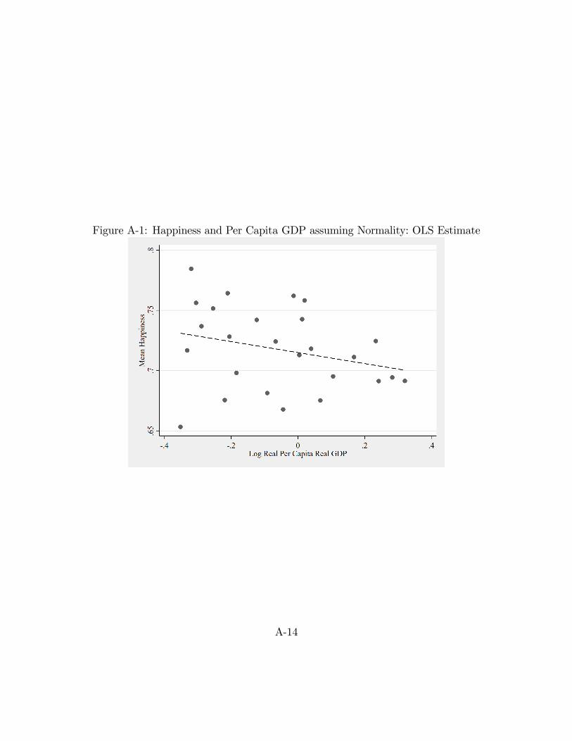
Figure A-1: Happiness and Per Capita GDP assuming Normality: OLS Estimate

A-14

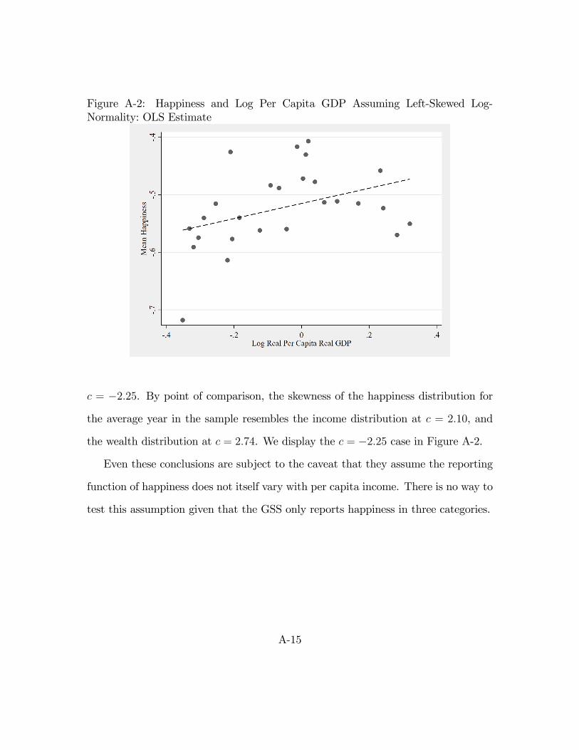
Figure A-2: Happiness and Log Per Capita GDP Assuming Left-Skewed Log-Normality: OLS Estimate

c = �2:25. By point of comparison, the skewness of the happiness distribution for

the average year in the sample resembles the income distribution at c = 2:10, and

the wealth distribution at c = 2:74. We display the c = �2:25 case in Figure A-2.

Even these conclusions are subject to the caveat that they assume the reporting

function of happiness does not itself vary with per capita income. There is no way to

test this assumption given that the GSS only reports happiness in three categories.

A-15

A.3.2 Happiness over the Lifecycle

There is a substantial literature that �nds happiness is U-shaped over the lifecycle.10

Individuals begin their adulthood fairly happy, see a decrease during much of their

working life, and then rebound in happiness as they reach retirement. Blanch�ower

and Oswald (2008) obtain this result across over 70 countries, and there is even

some evidence that it holds in apes (Weiss et al., 2012). This claim is, however, not

without controversy. In some data sets, the shape depends on the choice of control

variables, and whether one uses �xed e¤ects or a pooled regression (e.g., Glenn, 2009;

Kassenboehmer and Hasiken-DeNew, 2012).

Of course, such conclusions rely on particular cardinalization assumptions. To

test the robustness of these results to alternative cardinalizations, we utilize the

Eurobarometer, which as previously discussed uses a 4-point life satisfaction scale.

We restrict attention to men in the twelve members of the European Union as of

1986, as these countries have the most years of data. Following Blanch�ower and

Oswald (2008), we group individuals into 5 year age bins, although we group all

individuals over 80 into single bin due to the small number of people in this age

range.

We �rst ask whether it is possible to rank age groups by their mean happiness

without making any assumptions on the underlying distribution, applying the crite-

rion laid out in Section 2.1 of the main paper. In fact, it is not possible to rank any

two age groups within any country. All age-country groups have a positive number

10For some recent reviews, see Frijters and Beatton (2012), and Steptoe, Deaton, and Stone(2015)

A-16

of respondents in each category.

We then turn to whether we can rank age groups assuming that the distribution

of happiness is distributed normally within each country-age group. We estimate an

ordered probit for each country allowing the means and standard deviations to di¤er

by age group. In Figure A-3, we plot the lowess smoothed results of this exercise.

To emphasize the shape of the patterns, we normalize both sets of estimates to be

distributed with mean 0 and standard deviation 1 within country. We observe a U-

shaped pattern of means in a majority of countries, although it is more pronounced

in some than others. West Germany and Luxembourg appear more consistent with

an upward sloping age-happiness pro�le, while Portugal is more consistent with a

downward sloping pro�le.11

However, these conclusions about the age-happiness pro�le in means are inde-

pendent of cardinalization choice only if the variances are constant with age. While

there is no consistent pattern across countries in the age-standard deviation pro�le,

there is clear variation across age groups. In West Germany, Denmark, Greece, and

the Netherlands, the standard deviation of happiness appears to increase in age.

Luxembourg, Italy, and Spain are more consistent with a U-shape. France, Ireland,

and Portugal in contrast seem to have a relatively stable relation between age and

the variance of happiness. A joint test of the standard deviation being independent

of age in these countries yields a �2156-statistic of 545; we can reject the hypothesis

at any conventional signi�cance level.

Since, under the assumption of normality, the variance of happiness changes with

11The Eurobarometer continued to survey the areas of the former West Germany as a separateunit after reunifcation.

A-17

Figure A-3: Mean and Standard Devation of Happiness under Normal Cardinaliza-tion

A-18

age, alternative cardinalizations will yield di¤erent patterns in the means. Given the

average variance across country-years, a transformation of c = 4=3 would provide

similar skewness to the wealth distribution. We plot the age-happiness pro�le by

country under the left-skewed and right-skewed version of this cardinalization, as

well as the normal, in Figure A-4. We again subtract the average age-group mean

and divide by the standard deviation of these averages within country and transfor-

mation (so that our estimates have a distribution of mean 0, standard deviation 1)

to ease comparison of the shapes. The patterns di¤er dramatically under di¤erent

cardinalizations. Italy, and the Netherlands, which are U-shaped under the normal,

become downward sloping with a left-skewed transformation. This same transforma-

tion moves West Germany from upward sloping to hump-shaped. Denmark, which

was approximately U-shaped under the normal, is monotonically upward sloping un-

der a right-skewed transformation and monotonically downward under a left. The

United Kingdom gains a stronger U-shape when left-skewed, but becomes closer to

hump-shaped under a right. In contrast, Spain, France, Ireland, and Portugal have

fairly stable relations across transformations, though di¤erent patterns from each

other.

There are many equally plausible conclusions one could draw from Figure A-

4. If we had a strong prior that happiness is always normally distributed within

age group and country, then we would believe that most countries have U-shaped

happiness/age pro�les but that Portugal, Luxembourg, and West Germany violate

this pattern. If we had a strong belief that happiness follows a U-shape across the

lifecycle (and that the skewness of the distribution does not change with age), then

A-19

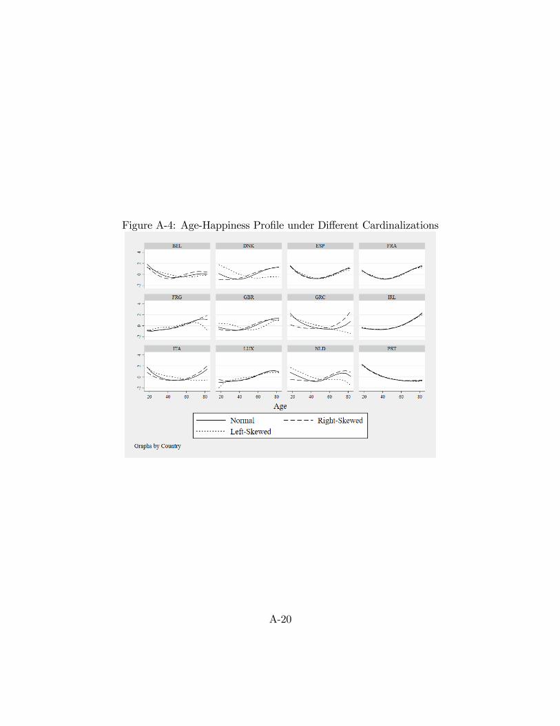
Figure A-4: Age-Happiness Pro�le under Di¤erent Cardinalizations

A-20

we would have to conclude that happiness is right-skewed in Luxembourg, but must

not be in Denmark. In the absence of any prior, we might conclude that Spain,

France, Portugal, and Ireland have a well-determined happiness/age relation, but

that we lack su¢ cient evidence to say anything with con�dence about the other EU

countries

However any such conclusions would have to be made with a giant caveat; they

assume a stable relation between experienced happiness and reported happiness

throughout the life-cycle. An alternative view of Figure A-4 might state that hap-

piness is constant throughout the lifecycle, but that in most EU countries, middle

aged-individuals have a higher standard for reporting satisfaction with their life.

Fortunately, this hypothesis is testable with the 4-category life satisfaction question

under the maintained assumption that happiness can be cardinalized to be in the

normal family (including the log normal).

In Figure A-5, we plot the implied thresholds (normalizing the �rst two cuto¤s to

be zero and one) from a series of ordered probits for reporting life satisfaction in the

highest threshold across age and country. While we again see no consistent pattern

in the relation between age and reporting function across countries, we see sub-

stantial variation within countries. To test formally for reporting function stability,

we perform a likelihood ratio test between these ordered probits and the country-

speci�c ordered probits that allow for the mean and standard deviation of happiness

to vary with age but forces the highest cuto¤ to be stable.12 This test generates a

�2156-statistic of 195, and we can reject stable reporting functions at the 5% level.

12In other words, we test a model where the reporting function is age- and country-speci�c againsta model where the reporting function is country-speci�c.

A-21

Figure A-5: Variation in the Reporting Function across Age Groups under Normality

A-22

A.3.3 The Unemployment-In�ation Trade-o¤

Many happiness researchers have advocated evaluating policy based on its ability to

raise the �average�response on measures of subjective well-being. The application

that has perhaps received the most widespread interest is correcting the misery in-

dex. While the misery index was developed as a political slogan, the idea that both

unemployment and in�ation are costly is intuitive. But it is by no means obvious

that the proper weights, even assuming linearity, are equal.

Di Tella, MacCulloch, and Oswald (2001, hereafter DMO) provide one prominent

attempt to use subjective well-being data to determine the appropriate trade-o¤

between unemployment and in�ation. They match estimated national well-being

from happiness surveys with time-series data on in�ation and unemployment across

countries. They �nd that both unemployment and in�ation are negatively related to

national happiness but that the cost of unemployment is 1.7 times that of in�ation.

Thus the politically-derived �misery index� (in�ation plus unemployment) biases

policy towards too much unemployment relative to in�ation.

To explore the robustness of this result, we follow DMO and use happiness data

from the Eurobarometer Trend File, and national unemployment and in�ation data

from the Organisation for Economic Co-operation and Development (OECD). DMO

study the time period 1975-1991. However, the OECD currently only o¤ers harmo-

nized unemployment data for European nations beginning in 1983.13 We therefore

focus on 1983-2002, which is slightly later than DMO but of similar duration. We

13These data are also not complete. For example, most countries have no data until they enterthe European Union, while Greece (which we exclude because of sample size) is not available until1999.

A-23

exclude any country which we observe for fewer than 6 years, since our method

requires the estimation of 5 parameters: e¤ects of in�ation and unemployment on

both the mean and the variance of life satisfaction, and the threshold for reporting

life satisfaction in the highest category. This yields a sample of 14 countries: Aus-

tria, Belgium, Denmark, Spain, Finland, France, Ireland, Italy, Luxembourg, the

Netherlands, Norway, Portugal, Sweden, and the United Kingdom.

Making a determination on the appropriate calibration of the misery index re-

quires much stronger conditions than those we consider in the main text. An e¤ort to

evaluate the e¤ect of in�ation and unemployment must �rst be able to rank various

years based on their average happiness either absolutely or within a country. The

condition in Section 2.1 of the main text lays out when such comparisons are possi-

ble without making a distributional assumption. Analyzing the yearly data from the

Eurobarometer we �nd there is not a single year in which a single country had a sin-

gle life satisfaction category that did not have a positive number of responses. Thus

even determining if high unemployment years are less happy than low unemployment

years must rely on assumptions about the distribution of life satisfaction.

Assuming the existence of a normal cardinalization, we can at least determine

whether in�ation and/or unemployment lowers happiness provided that these vari-

ables do not in�uence the variance of happiness. To test for a constant variance,

for each country we estimate an ordered probit that allows the mean and variance

to be a¤ected by in�ation and unemployment. We then perform a joint test that

neither in�ation nor unemployment has any e¤ect on the variance of happiness in

any country in our sample. This yields a �228-statistic of 611, and we can easily

A-24

reject the null hypothesis at any conventional level. Thus even the statement that

the national unemployment and in�ation rates lower average life satisfaction, a much

weaker statement than the optimal policy trade-o¤ between in�ation and unemploy-

ment, is only true for some cardinalizations of happiness.

To explore conclusions that can be drawn from alternative distributional as-

sumptions, we �rst estimate country-speci�c heteroskedastic ordered probits using

individual-level data on life satisfaction from the Eurobarometer Trend File. In these

regressions we control for marital status, education, a quadratic in age, and a set

of year dummies.14 From these, we calculate the mean and standard deviation of

happiness in each country in each year (at the mean of our controls in the EU) using

the estimated coe¢ cients on the year dummies by the method discussed in section

A.1. We then follow DMO by estimating a pooled regression of mean happiness on

annual unemployment, in�ation, a set of year �xed e¤ects, country �xed e¤ects, and

country-speci�c time trends, which represents DMO�s preferred speci�cation.15 We

also estimate this regression under alternative right-skewed and left-skewed trans-

formations of happiness. To provide comparability across estimates, we normalize

each transformation so that the distribution of happiness is mean zero with standard

deviation one across country-years.

14Unlike DMO, we do not control for unemployment status in these �rst stage regressions. Thiswould cause our second stage to understate the true welfare cost of national unemployment. DMOrecognize this problem and adjust their results using the estimated e¤ect of unemployment onhappiness in the �rst stage. However, changes in the distribution of happiness will also change theestimated e¤ect of unemployment on individual-level happiness, so performing such an adjustmentwould be inappropriate in our context.15DMO use 3-year moving averages of in�ation and unemployment rather than the annual values.

It is not clear whether this is due to a data limitation or a preference for smoothing year-to-yearvariation in these variables. We use the annual �gures as our results more closely resemble DMO�sunder a normal distribution than when using 3-year moving averages.

A-25

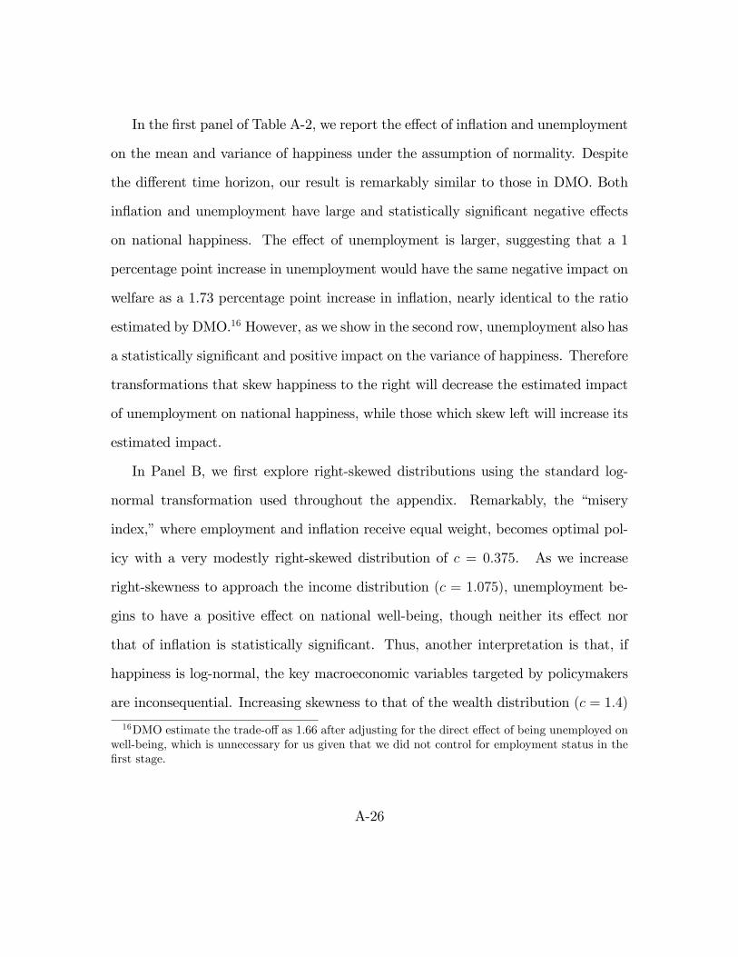
In the �rst panel of Table A-2, we report the e¤ect of in�ation and unemployment

on the mean and variance of happiness under the assumption of normality. Despite

the di¤erent time horizon, our result is remarkably similar to those in DMO. Both

in�ation and unemployment have large and statistically signi�cant negative e¤ects

on national happiness. The e¤ect of unemployment is larger, suggesting that a 1

percentage point increase in unemployment would have the same negative impact on

welfare as a 1.73 percentage point increase in in�ation, nearly identical to the ratio

estimated by DMO.16 However, as we show in the second row, unemployment also has

a statistically signi�cant and positive impact on the variance of happiness. Therefore

transformations that skew happiness to the right will decrease the estimated impact

of unemployment on national happiness, while those which skew left will increase its

estimated impact.

In Panel B, we �rst explore right-skewed distributions using the standard log-

normal transformation used throughout the appendix. Remarkably, the �misery

index,�where employment and in�ation receive equal weight, becomes optimal pol-

icy with a very modestly right-skewed distribution of c = 0:375. As we increase

right-skewness to approach the income distribution (c = 1:075), unemployment be-

gins to have a positive e¤ect on national well-being, though neither its e¤ect nor

that of in�ation is statistically signi�cant. Thus, another interpretation is that, if

happiness is log-normal, the key macroeconomic variables targeted by policymakers

are inconsequential. Increasing skewness to that of the wealth distribution (c = 1:4)

16DMO estimate the trade-o¤ as 1.66 after adjusting for the direct e¤ect of being unemployed onwell-being, which is unnecessary for us given that we did not control for employment status in the�rst stage.

A-26

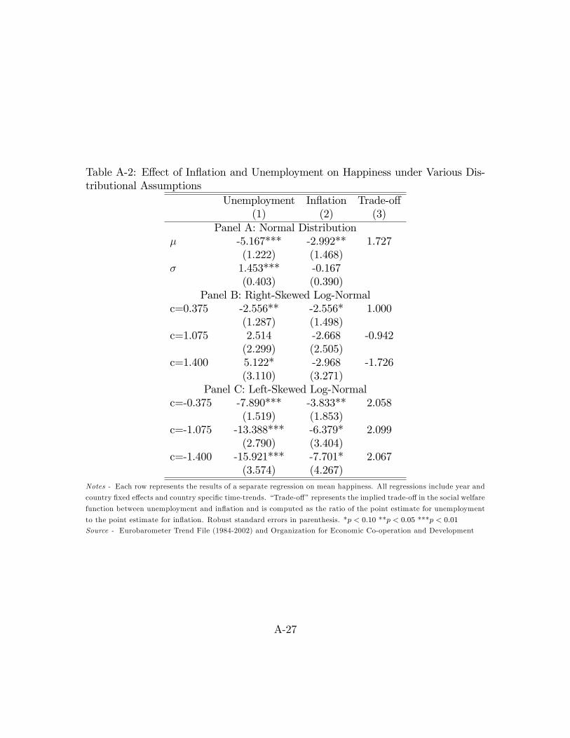
Table A-2: E¤ect of In�ation and Unemployment on Happiness under Various Dis-tributional Assumptions

Unemployment In�ation Trade-o¤(1) (2) (3)

Panel A: Normal Distribution� -5.167*** -2.992** 1.727

(1.222) (1.468)� 1.453*** -0.167

(0.403) (0.390)Panel B: Right-Skewed Log-Normal

c=0.375 -2.556** -2.556* 1.000(1.287) (1.498)

c=1.075 2.514 -2.668 -0.942(2.299) (2.505)

c=1.400 5.122* -2.968 -1.726(3.110) (3.271)

Panel C: Left-Skewed Log-Normalc=-0.375 -7.890*** -3.833** 2.058

(1.519) (1.853)c=-1.075 -13.388*** -6.379* 2.099

(2.790) (3.404)c=-1.400 -15.921*** -7.701* 2.067

(3.574) (4.267)Notes - Each row represents the results of a separate regression on mean happiness. All regressions include year and

country �xed e¤ects and country speci�c time-trends. �Trade-o¤�represents the implied trade-o¤ in the social welfare

function between unemployment and in�ation and is computed as the ratio of the point estimate for unemployment

to the point estimate for in�ation. Robust standard errors in parenthesis. *p < 0:10 **p < 0:05 ***p < 0:01

Source - Eurobarometer Trend File (1984-2002) and Organization for Economic Co-operation and Development

A-27

makes the positive e¤ect of unemployment statistically signi�cant, consistent with

arguments that recessions are �good for your health�(Ruhm 2000).

In contrast, as we show in Panel C, when we allow happiness to become left-

skewed, unemployment becomes more important for well-being. At c = �0:375,

a one percentage point increase in unemployment lowers happiness by 2.05 times

as much as a one percentage point increase in in�ation, and similarly 2.1 times at

c = �1:075 and 2.07 times at c = �1:4.

On a somewhat optimistic note, our results make intuitive sense. We would ex-

pect that unemployment would generally make people less happy, a result consistent

with a large literature using self-reported happiness (e.g. Clark and Oswald, 1994;

Blanch�ower, 2001; Blanch�ower and Oswald, 2004). It is at least plausible that

those who are most directly a¤ected by unemployment are located in the left-tail

of the happiness distribution. Increasing the left-skewness of happiness is equiva-

lent to using a social welfare function that places more weight on the least happy

individuals relative to the happiest. When unemployment increases, there are more

unhappy unemployed individuals, and the more weight we place on these individu-

als, the larger the social cost will appear. In contrast, a right-skewed transformation

increases the weight on the happiest individuals relative to the least happy. Since the

happiest people will disproportionately hold stable jobs, increases in unemployment

are unlikely to bother them. Even a positive e¤ect of unemployment is plausible for

a highly right-skewed social welfare function if, as some have suggested, individuals

report happiness based on their relative circumstances.17 When many are without a

17See Clark, Frijters, and Shields (2008) for a review of the empirical evidence that social com-parisons are important for happiness.

A-28

job, those still employed may report particularly high levels of happiness.18

Even if there were some strong a priori reason to adopt a speci�c cardinalization,

these results would still require the assumption that the reporting function itself is

stable across time. This assumption is testable as the Eurobarometer life-satisfaction

questions uses a 4-point scale. Applying the method discussed in section A.1.4,

we perform a likelihood ratio test for equal reporting functions across year within

country, and construct the joint test across these countries. That is we allow the

reporting function to vary across country, but not within, an even weaker assumption

than that required to estimate Table A-2. This yields a �2197-statistic of 491, and

we can thus strongly reject the hypothesis that the data support the existence of a

normal cardinalization with a stable reporting function across time.

A.3.4 Cross-Country Comparisons

In previous sections we found that the ranking of happiness across groups is highly

sensitive to distributional assumptions. To explore this sensitivity in a larger context,

we use the WVS to rank nations based on mean happiness. Constructing such a

ranking without a distributional assumption requires the data to satisfy the condition

from section 2.1 in the main text. Looking at the distribution of responses by country,

remarkably none of the 1,300 Malaysian respondents report being �not at all happy�

with their life. However, every other country�s respondents utilize every category;

consequently, we still are unable to rank Malaysia against any other country or to

18While Clark (2003) presents evidence that macro-level unemployment has a negative impacton the average well-being of the employed, this does not necessarily mean that macro-level unem-ployment has a negative impact on the well-being of the happiest employed individuals, who wouldbe weighted most heavily by a right-skewed social welfare function.

A-29

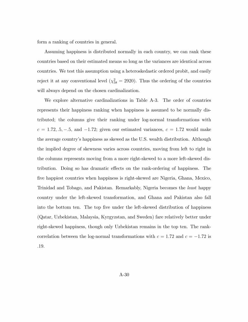
form a ranking of countries in general.

Assuming happiness is distributed normally in each country, we can rank these

countries based on their estimated means so long as the variances are identical across

countries. We test this assumption using a heteroskedastic ordered probit, and easily

reject it at any conventional level (�258 = 2920). Thus the ordering of the countries

will always depend on the chosen cardinalization.

We explore alternative cardinalizations in Table A-3. The order of countries

represents their happiness ranking when happiness is assumed to be normally dis-

tributed; the columns give their ranking under log-normal transformations with

c = 1:72; :5;�:5; and �1:72; given our estimated variances, c = 1:72 would make

the average country�s happiness as skewed as the U.S. wealth distribution. Although

the implied degree of skewness varies across countries, moving from left to right in

the columns represents moving from a more right-skewed to a more left-skewed dis-

tribution. Doing so has dramatic e¤ects on the rank-ordering of happiness. The

�ve happiest countries when happiness is right-skewed are Nigeria, Ghana, Mexico,

Trinidad and Tobago, and Pakistan. Remarkably, Nigeria becomes the least happy

country under the left-skewed transformation, and Ghana and Pakistan also fall

into the bottom ten. The top �ve under the left-skewed distribution of happiness

(Qatar, Uzbekistan, Malaysia, Kyrgyzstan, and Sweden) fare relatively better under

right-skewed happiness, though only Uzbekistan remains in the top ten. The rank-

correlation between the log-normal transformations with c = 1:72 and c = �1:72 is

:19.

A-30

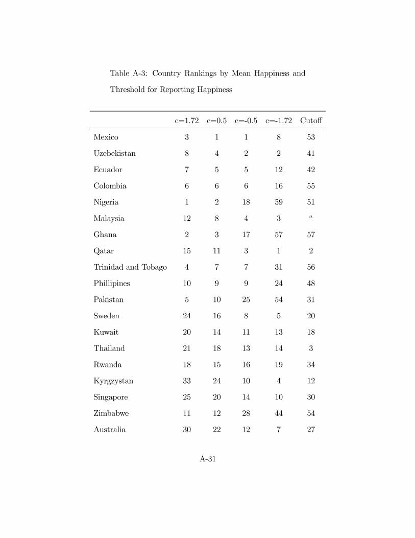
Table A-3: Country Rankings by Mean Happiness and

Threshold for Reporting Happiness

c=1.72 c=0.5 c=-0.5 c=-1.72 Cuto¤

Mexico 3 1 1 8 53

Uzebekistan 8 4 2 2 41

Ecuador 7 5 5 12 42

Colombia 6 6 6 16 55

Nigeria 1 2 18 59 51

Malaysia 12 8 4 3 a

Ghana 2 3 17 57 57

Qatar 15 11 3 1 2

Trinidad and Tobago 4 7 7 31 56

Phillipines 10 9 9 24 48

Pakistan 5 10 25 54 31

Sweden 24 16 8 5 20

Kuwait 20 14 11 13 18

Thailand 21 18 13 14 3

Rwanda 18 15 16 19 34

Kyrgzystan 33 24 10 4 12

Singapore 25 20 14 10 30

Zimbabwe 11 12 28 44 54

Australia 30 22 12 7 27

A-31

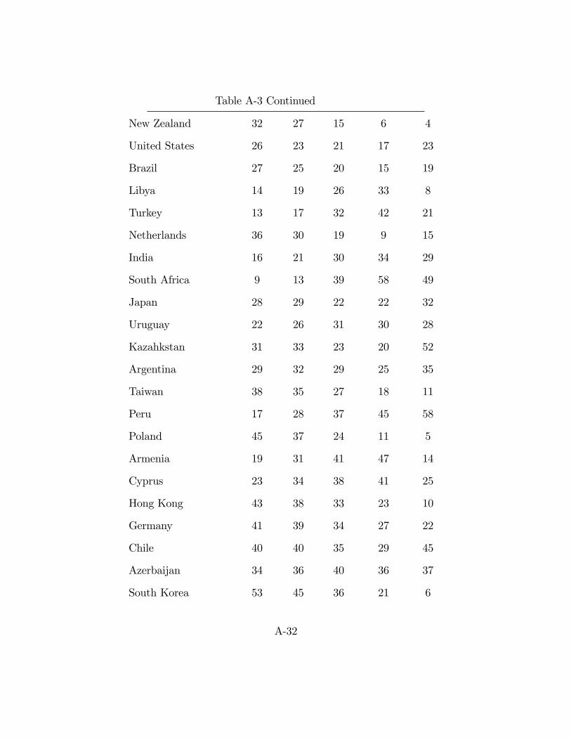
Table A-3 Continued

New Zealand 32 27 15 6 4

United States 26 23 21 17 23

Brazil 27 25 20 15 19

Libya 14 19 26 33 8

Turkey 13 17 32 42 21

Netherlands 36 30 19 9 15

India 16 21 30 34 29

South Africa 9 13 39 58 49

Japan 28 29 22 22 32

Uruguay 22 26 31 30 28

Kazahkstan 31 33 23 20 52

Argentina 29 32 29 25 35

Taiwan 38 35 27 18 11

Peru 17 28 37 45 58

Poland 45 37 24 11 5

Armenia 19 31 41 47 14

Cyprus 23 34 38 41 25

Hong Kong 43 38 33 23 10

Germany 41 39 34 27 22

Chile 40 40 35 29 45

Azerbaijan 34 36 40 36 37

South Korea 53 45 36 21 6

A-32

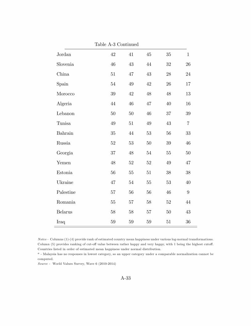
Table A-3 Continued

Jordan 42 41 45 35 1

Slovenia 46 43 44 32 26

China 51 47 43 28 24

Spain 54 49 42 26 17

Morocco 39 42 48 48 13

Algeria 44 46 47 40 16

Lebanon 50 50 46 37 39

Tunisa 49 51 49 43 7

Bahrain 35 44 53 56 33

Russia 52 53 50 39 46

Georgia 37 48 54 55 50

Yemen 48 52 52 49 47

Estonia 56 55 51 38 38

Ukraine 47 54 55 53 40

Palestine 57 56 56 46 9

Romania 55 57 58 52 44

Belarus 58 58 57 50 43

Iraq 59 59 59 51 36

Notes - Columns (1)-(4) provide rank of estimated country mean happiness under various log-normal transformations.

Column (5) provides ranking of cut-o¤ value between rather happy and very happy, with 1 being the highest cuto¤.

Countries listed in order of estimated mean happiness under normal distribution.a - Malaysia has no responses in lowest category, so an upper category under a comparable normalization cannot be

computed.

Source - World Values Survey, Wave 6 (2010-2014)

A-33

Figure A-6: Distribution of Thresholds for Reporting "Very Happy" under Normality

There are some countries whose rank remains fairly stable across the transforma-

tions. Uzbekistan is the second happiest country under a normal distribution and its

rank varies between 2 and 8 under the skewed distributions. Iraq, the world�s least

happy country under the normal distribution, is never able to rise out of the bottom

ten in the skewed transformations. These cases are counterbalanced by countries

like the previously mentioned Nigeria, as well as South Africa, which falls near the

middle of the distribution when happiness is normally distributed, is able to rise as

high as 7th when happiness is right-skewed, but falls all the way to 3rd lowest when

happiness is left-skewed.

All of these rankings relied on the reporting function of happiness being stable

across countries, a heroic assumption in light of the questionnaires being administered

A-34

in a large number of di¤erent languages. In Figure A-6, we relax the common report-

ing function assumption and construct a density plot of the thresholds for reporting

in the highest happiness category. The variation is substantial. Using a likelihood

ratio test, we can strongly reject common reporting functions at any conventional

level (�258 = 593). The �fth column of Table A-2 ranks our countries from highest to

lowest based on their threshold for reporting being very happy, assuming normality.

The happiest countries in our normal ranking were substantial benefactors of having

populations with low thresholds for reporting �very happy�; 3 of the top 5 ranked in

the bottom 10 for cuto¤s, while the two others ranked in the bottom twenty. On the

other hand, Qatar�s 8th ranking under normality appears quite remarkable given its

residents had the second highest standard for reporting in the top category.

A.3.5 Moving to Opportunity

Happiness data have also been used to evaluate micro-level policies, as in the case

of the Moving to Opportunity (MTO) program. Motivated by the positive results

of the Gautreaux desegregation program in Chicago, the MTO experiment targeted

families living in public housing in high poverty areas.19 Eligible families were invited

to apply for the chance to receive a Section 8 housing (rental assistance) voucher.

Applicants were randomly assigned to three groups: no voucher (Control group),

Section 8 voucher that could only be used in an area with a poverty rate below 10%

(Experimental group), and a standard Section 8 voucher (Section 8 group). The

19The Gautreaux program came out of a court-ordered desegration program in Chicago in the1970s. See Rosenbaum (1995) for a detailed analysis.

A-35

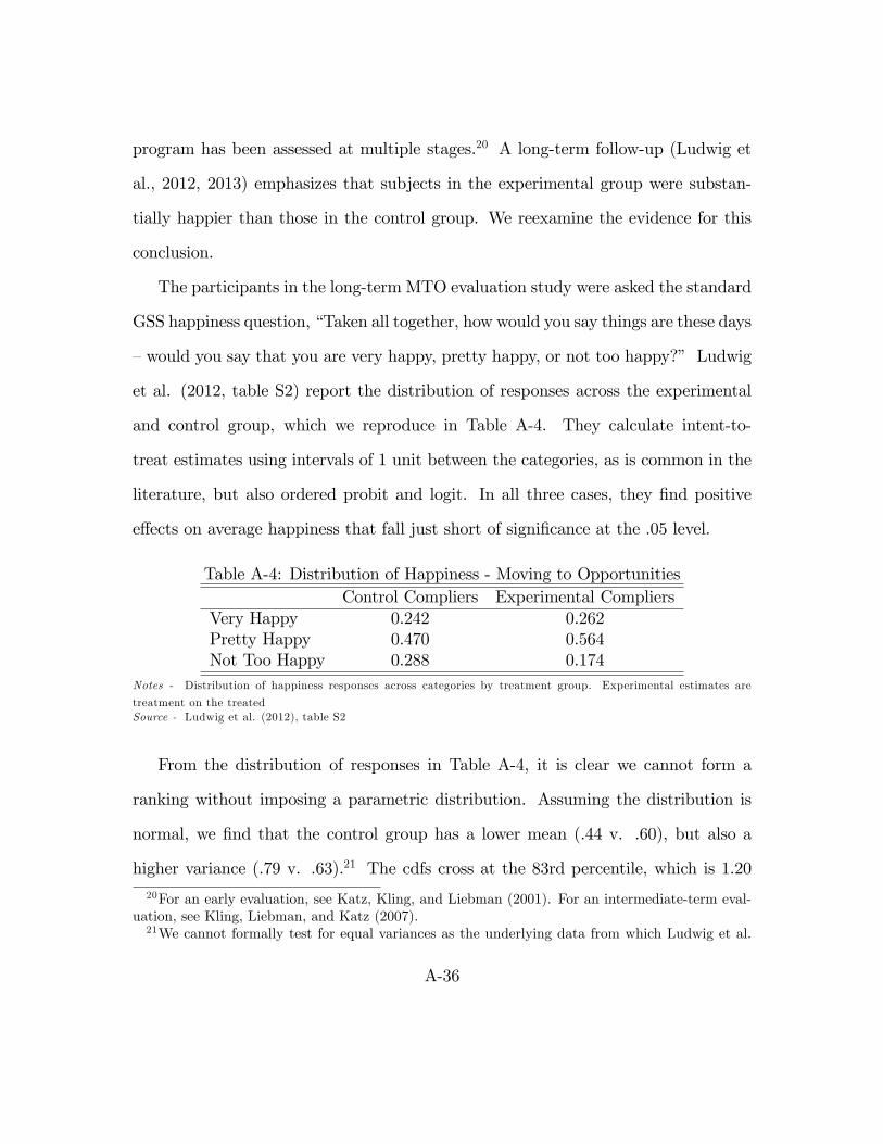
program has been assessed at multiple stages.20 A long-term follow-up (Ludwig et

al., 2012, 2013) emphasizes that subjects in the experimental group were substan-

tially happier than those in the control group. We reexamine the evidence for this

conclusion.

The participants in the long-term MTO evaluation study were asked the standard

GSS happiness question, �Taken all together, how would you say things are these days

�would you say that you are very happy, pretty happy, or not too happy?� Ludwig

et al. (2012, table S2) report the distribution of responses across the experimental

and control group, which we reproduce in Table A-4. They calculate intent-to-

treat estimates using intervals of 1 unit between the categories, as is common in the

literature, but also ordered probit and logit. In all three cases, they �nd positive

e¤ects on average happiness that fall just short of signi�cance at the .05 level.

Table A-4: Distribution of Happiness - Moving to OpportunitiesControl Compliers Experimental Compliers

Very Happy 0.242 0.262Pretty Happy 0.470 0.564Not Too Happy 0.288 0.174

Notes - Distribution of happiness responses across categories by treatment group. Experimental estimates are

treatment on the treatedSource - Ludwig et al. (2012), table S2

From the distribution of responses in Table A-4, it is clear we cannot form a

ranking without imposing a parametric distribution. Assuming the distribution is

normal, we �nd that the control group has a lower mean (.44 v. .60), but also a

higher variance (.79 v. .63).21 The cdfs cross at the 83rd percentile, which is 1.2020For an early evaluation, see Katz, Kling, and Liebman (2001). For an intermediate-term eval-

uation, see Kling, Liebman, and Katz (2007).21We cannot formally test for equal variances as the underlying data from which Ludwig et al.

A-36

units of happiness (and also in the extreme left tail of the distributions). Thus if we

simply transform the underlying happiness data to increase the values above 1.20 we

can reverse the mean happiness. This cardinalization would explain the data equally

well.

Since the control group has a higher variance of happiness, it will be possible to

reverse this result by applying a right-skewed distribution. From our point estimates,

the required transformation is just slightly more skewed than a standard log-normal;

we need only apply a c = 1:33. We plot the resulting distributions in Figure A-7.

Both distributions are less skewed than the income distribution, with the mean of the

control group lying at the 70th percentile, and the mean of the experimental group at

the 72nd percentile. One plausible interpretation of the data is that moving to a low

poverty area increased happiness for most people, but that there is a group of people

who were extremely happy in their old environment who could not match positive

aspects of their former social environment in their new community. Of course, this

all assumes that moving to a new environment did not in�uence the way in which

individuals report their happiness, a possible scenario that is not testable given that

the happiness scale used by the researchers has only 3 points.

A.3.6 Marriage and Children

One of the most robust results in the happiness literature is that married individuals

are happier than non-married individuals. This phenomenon has been observed both

across countries and across time (e.g., Stack and Eshelman, 1998; Diener et. al, 2000;

(2012) calculated the distribution of their responses are not publicly available.

A-37

Figure A-7: MTO Log-Normal Happiness Distribution with Equal Means

A-38

Blanch�ower and Oswald, 2004).22 In contrast, happiness researchers generally �nd

that individuals with children are less happy than those without (e.g., Alesina et. al,

2004; Blanch�ower, 2009; Stanca, 2012; Deaton and Stone, 2015).23 These con�icting

results present a bit of a conundrum. As both getting married and having children

are actions that individuals (generally) take voluntarily, revealed preference suggests

they should both raise happiness although as Deaton and Stone (2015) point out, if

only people who expect children to make them happier become parents, in a cross-

section having children and happiness might be unrelated. Likewise, most parents

are unwilling to express publicly that their children are a source of unhappiness.

In this section we explore the robustness of cross-section comparisons between

those who are married and those who are not, and those who live with and without

children using the BHPS. We restrict attention to those aged 16-60 and separate

individuals by gender. In our analysis of married individuals, we exclude those who

are widowed, separated, or divorced; for our analysis of children we focus only on

those who are married.

We �rst ask if it is possible to make any comparison without assuming a functional

form for the distribution of happiness by comparing the distribution of responses

within each of these groups. In no case is this possible. Regardless of gender,

marital status, or child cohabitation status, we �nd in every case a positive number

of responses in every life satisfaction category. Therefore we cannot say anything

22Note this is a distinct question from whether marriage causes individuals to become happier,which is a much more controversial claim. Lucas et al. (2003), for instance, present evidenceconsistent with the idea that becoming married causes a short term increase in one�s well-being,but that the individual eventually �adapts�and returns to his or her pre-marital happiness.23There are important exceptions however. For example, Angeles (2010) �nds positive e¤ects of

children on the happiness of married individuals in Britain.

A-39

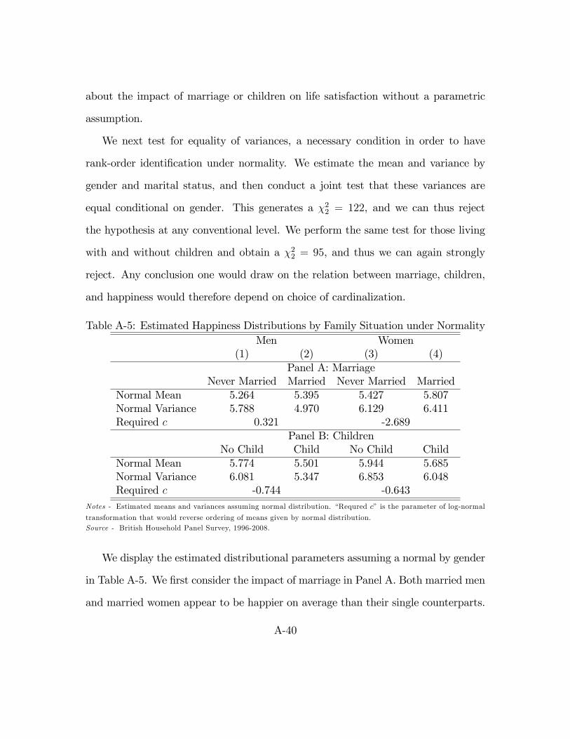
about the impact of marriage or children on life satisfaction without a parametric

assumption.

We next test for equality of variances, a necessary condition in order to have

rank-order identi�cation under normality. We estimate the mean and variance by

gender and marital status, and then conduct a joint test that these variances are

equal conditional on gender. This generates a �22 = 122, and we can thus reject

the hypothesis at any conventional level. We perform the same test for those living

with and without children and obtain a �22 = 95, and thus we can again strongly

reject. Any conclusion one would draw on the relation between marriage, children,

and happiness would therefore depend on choice of cardinalization.

Table A-5: Estimated Happiness Distributions by Family Situation under NormalityMen Women

(1) (2) (3) (4)Panel A: Marriage

Never Married Married Never Married MarriedNormal Mean 5.264 5.395 5.427 5.807Normal Variance 5.788 4.970 6.129 6.411Required c 0.321 -2.689

Panel B: ChildrenNo Child Child No Child Child

Normal Mean 5.774 5.501 5.944 5.685Normal Variance 6.081 5.347 6.853 6.048Required c -0.744 -0.643

Notes - Estimated means and variances assuming normal distribution. �Requred c� is the parameter of log-normal

transformation that would reverse ordering of means given by normal distribution.Source - British Household Panel Survey, 1996-2008.

We display the estimated distributional parameters assuming a normal by gender

in Table A-5. We �rst consider the impact of marriage in Panel A. Both married men

and married women appear to be happier on average than their single counterparts.

A-40

However, we also observe that married men have a lower variance of happiness than

single men. Thus, we can reverse this relationship with a right-skewed log-normal

transformation. The required transformation itself is quite modest; with c = :32,

single men become happier. By comparison, the distribution for single men would

not reach the skewness of the income distribution until c = :54. In contrast, married

women appear to have a higher variance of life satisfaction than single women. We

thus require a left-skewed log-normal to reverse. For any c � �2:69, we would

conclude that single women are happier than married women. These distributions

are skewed substantially to the left; the mean of married women lies within the .1th

percentile. However, transformations outside the lognormal family could certainly

reverse the result with less skewness, and there is no particular reason to believe that

getting married does not itself a¤ect the skewness of happiness.

In Panel B, we turn to the impact of children on life satisfaction. Consistent with

most of the literature, we �nd that, assuming normality, both men and women who

live with children are less happy than those who do not. However, in both cases we

estimate that individuals living without children have a higher variance of happiness

than those living with children. Thus, we can reverse these results with a left-skewed

log normal. The required transformations are similar, for men we require c = �:74,

for women c = �:64, and produce distributions with skewness similar to the wealth

distribution of the United States (though in the opposite direction).24

Finally all of these results assume a common reporting function. It is plausible

24Under the reversing transformations, the mean of the child-less male distribution falls in the18th percentile, 19th percentile for male with child, 20th percentile for child-less female, and 21stpercentile for female with child.

A-41

that marriage and having children change the way that people report their happiness.

Because the BHPS measures life satisfaction on a 7-point scale, this assumption is

testable. For each of our outcomes, we perform a likelihood ratio test of equality of

the reporting function for men and women separately, and then calculate the joint

test. That is, our null hypothesis allows gender, but not family status, to a¤ect the

reporting of happiness. For marital status, our resulting test statistic is �28 = 84;

for living with children we �nd �28 = 21. We can thus reject a common reporting

function for both cases at the 1%-level.

A.3.7 The Paradox of Declining Female Happiness

One surprising result from the happiness literature, documented by Stevenson and

Wolfers (2009), is that in the United States women�s happiness appears to have fallen

relative to men�s from 1972-2006 despite the great social and economic progress

women made during this period.25 We explore the robustness of this result using

these same data.

Fundamentally, the question seeks to order the average happiness of women�s

happiness by year relative to men. As discussed previously a necessary (but not

su¢ cient) condition to be able to make such a comparison without imposing a distri-

butional assumption on happiness is that there are some groups which never report

in the highest category, and some which never report in the lowest. Analyzing the

data year by year, we see this criterion is never met for men or women in any year

25By labeling this �surprising,�we do not mean to imply that it could not be true. In a relatedarea, Black et al. (2009) suggest that apparent black-white earnings convergence was accompaniedby black mobility to higher cost localities, suggesting much less convergence in real incomes.

A-42

of the GSS. Thus comparisons cannot be made without distributional assumptions,

and any conclusion will rest on the functional form assumed.

If we are willing to assume a cardinalization exists in which, in each year of the

data, both men and women�s happiness is distributed normally, we can make com-

parisons that are robust to any alternative cardinalization provided the variance is

constant across all years for each gender. Using a heteroskedastic ordered probit,

we estimate the means and standard deviation of happiness by gender for each year

assuming normality and test whether the standard deviation is constant. This gen-

erates a �251 = 144, and we can reject equality of variances at any conventional level

of statistical signi�cance. Thus conclusions about trends in relative male to female

happiness will depend on the cardinalization chosen by the researcher.

In Figure A-8 we plot the mean happiness for men and women under the normal-

ity assumption. Consistent with Stevenson and Wolfers, we see a sharp decline in

women�s happiness, while men�s remains relatively constant, indicating that under

this cardinalization, women have lost ground relative to men. However, in Figure

A-9, we plot the standard deviations across time, and consistent with our above test,

�nd substantial changes here as well. While the standard deviation has generally

declined for both genders, women�s has fallen relative to men�s. Thus the pattern in

means can be reversed by a left-skewed log-normal.

In Figure A-10 we plot the estimated linear (10-year) trend in relative happiness

from an OLS regression as a function of the c chosen in the left-skewed log-normal

along with the 95% con�dence interval. As we add more skewness, the trend begins

to favor men less and women more. By c = �:35, the trend is already statistically

A-43

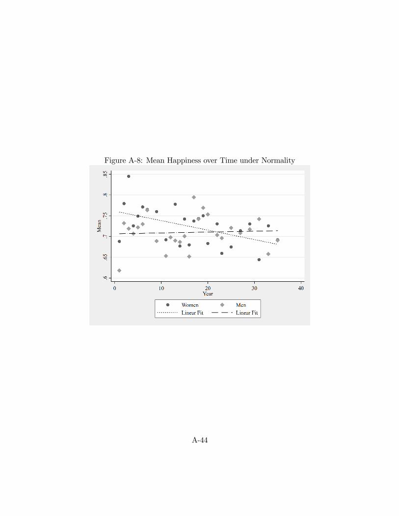
Figure A-8: Mean Happiness over Time under Normality

A-44

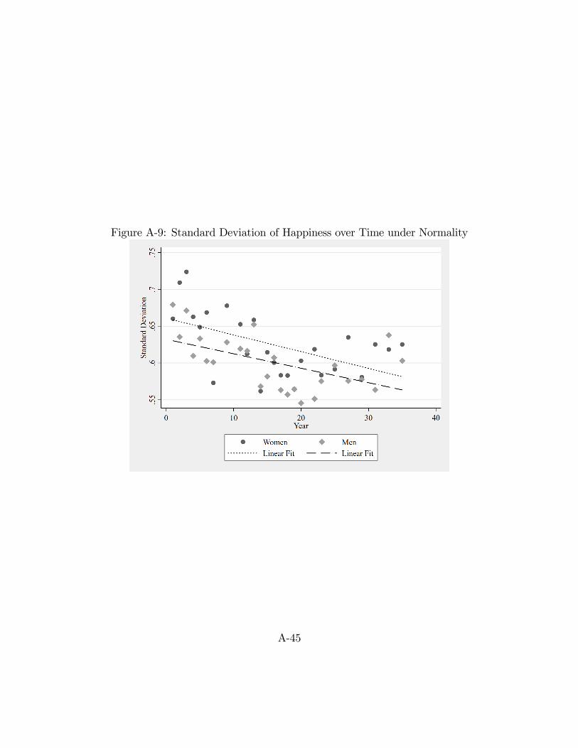
Figure A-9: Standard Deviation of Happiness over Time under Normality

A-45

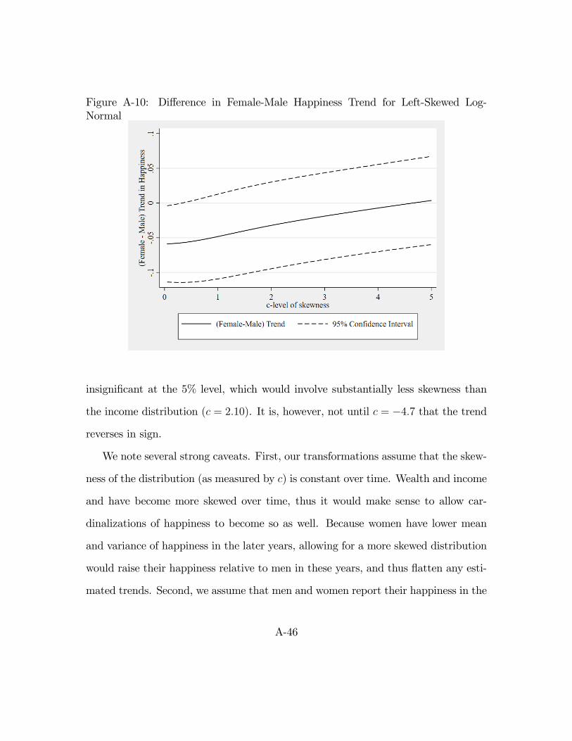
Figure A-10: Di¤erence in Female-Male Happiness Trend for Left-Skewed Log-Normal

insigni�cant at the 5% level, which would involve substantially less skewness than

the income distribution (c = 2:10). It is, however, not until c = �4:7 that the trend

reverses in sign.

We note several strong caveats. First, our transformations assume that the skew-

ness of the distribution (as measured by c) is constant over time. Wealth and income

and have become more skewed over time, thus it would make sense to allow car-

dinalizations of happiness to become so as well. Because women have lower mean

and variance of happiness in the later years, allowing for a more skewed distribution

would raise their happiness relative to men in these years, and thus �atten any esti-

mated trends. Second, we assume that men and women report their happiness in the

A-46

same way, and that the way in which they report their happiness does not change

overtime. An equally plausible explanation is that over time the social and economic

progress made by women has led them to raise the standard with which they evalu-

ate happiness, which would arti�cially lower their reported happiness. Because the

GSS only measures happiness on a 3-point scale, we cannot test for changes in the

reporting function.

A.3.8 Adaptation to Disability

One of the most striking results in the happiness literature is the �nding that people

adapt to disability. Kahneman (2011) suggests that the experienced utility of para-

plegics and nonparaplegics is fairly similar after a period of adaptation. Whether

adaptation is complete is controversial, but partial adaptation is widely accepted.

For example, Oswald and Powdthavee (2008) argue that the widely cited Brickman

et al. (1978) study has been misinterpreted and also �nd notable but only partial re-

covery of happiness from what they de�ne as moderate and severe disability. Yet the

question of adaptation to disability and other adverse events is, perhaps, unusually

sensitive to concerns about the reporting function. Individuals may reconcile them-

selves to such events either by becoming less unhappy about them or by reducing

the standard for reporting themselves as happy.

We approach this question using the BHPS, which includes the measure on life

satisfaction discussed before and asks respondents about their disabilities. We note

there are some inconsistencies in the disability question across waves that we are

forced to ignore in the interest of having an adequate time series. From 1996 to

A-47

2000, we use the question �Can I check, are you registered as a disabled person,

either with Social Services or with a green card?�For 2002 and 2003, we use �Can I

check, are you registered as a disabled person?�Finally, from 2004 on, we use �Can

I check, do you consider yourself to be a disabled person?�On the face of things, we

would expect the largest di¤erence to be between 2003 and 2004 when the question

shifts from being purely factual to one of self-image. In fact the di¤erence between

2002-3 and 2004-8 is negligible. There is a large jump between 2000 and 2002, but

this seems largely to re�ect an upward trend between 1996 and 2002.

Unfortunately, the BHPS does not have a large enough sample of long-term dis-

abled individuals to test for adaptation within an individual. Instead, we construct

a sample of individuals who ever report being disabled, and compare the distribution

of responses in years where these individuals were disabled with the distribution of

responses in years where they were not. We limit the sample to individuals ages

16 to 60, and exclude anyone who was disabled upon entering the sample. If the

information on disability was missing in any given year, we used the response from

the previous year or, if that was missing either because of non-response or because

the missing year was the respondent�s �rst in the sample, we use the response from

the following year. Any remaining missing cases were recoded as not disabled.

We �rst test if it is possible to conclude whether disabled years were less happy

than non-disabled years (or vice-versa). Comparing the distribution of categorical

responses, we observe that both the disabled and the non-disabled utilize all of the

seven categories of life satisfaction. Thus, under the condition derived in section 2.1

of the main text, it is not possible to determine whether the disabled or non-disabled

A-48

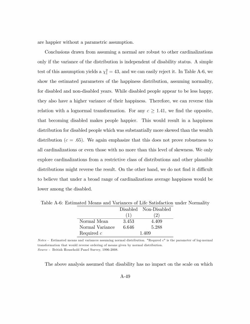
are happier without a parametric assumption.

Conclusions drawn from assuming a normal are robust to other cardinalizations

only if the variance of the distribution is independent of disability status. A simple

test of this assumption yields a �21 = 43, and we can easily reject it. In Table A-6, we

show the estimated parameters of the happiness distribution, assuming normality,

for disabled and non-disabled years. While disabled people appear to be less happy,

they also have a higher variance of their happiness. Therefore, we can reverse this

relation with a lognormal transformation. For any c � 1:41, we �nd the opposite,

that becoming disabled makes people happier. This would result in a happiness

distribution for disabled people which was substantially more skewed than the wealth

distribution (c = :65). We again emphasize that this does not prove robustness to

all cardinalizations or even those with no more than this level of skewness. We only

explore cardinalizations from a restrictive class of distributions and other plausible

distributions might reverse the result. On the other hand, we do not �nd it di¢ cult

to believe that under a broad range of cardinalizations average happiness would be

lower among the disabled.

Table A-6: Estimated Means and Variances of Life Satisfaction under NormalityDisabled Non-Disabled(1) (2)

Normal Mean 3.453 4.409Normal Variance 6.646 5.288Required c 1.409

Notes - Estimated means and variances assuming normal distribution. "Requred c" is the parameter of log-normal

transformation that would reverse ordering of means given by normal distribution.Source - British Household Panel Survey, 1996-2008.

The above analysis assumed that disability has no impact on the scale on which

A-49

individuals report their happiness. As discussed above, an alternative theory to the

widely cited adaptation literature is that individuals adapt their reporting function.

Once disabled, they lower their thresholds for reporting the highest levels of life

satisfaction. Because the BHPS measures life satisfaction on a 7-point scale, we can

again test, under the maintained normal cardinalization, whether the disabled and

the non-disabled use the same reporting function. A likelihood ratio test generates a

�24 = 23, and thus we can reject equal reporting functions at any conventional level

of signi�cance.

In Table A-7, we report the estimated cuto¤ values for the latent life satisfaction

variable for reporting in the 7 di¤erent categories. The �rst two cuto¤ values are

normalized to be 0 and 1. We see strong evidence that disabled individuals have

lower standards for reporting satisfaction with their life, particularly for the highest

two cuto¤s. This suggests that applying the standard normality assumption will

�rst lead us to underestimate the negative e¤ects of disability on happiness, and

second to overestimate adaptation to disability. At least some �adaptation�comes

from changes in the reporting function rather than the true level of happiness.

Table A-7: Estimated Cutpoints under NormalityDisabled Not Disabled(1) (2)

1 to 2 0 02 to 3 1 13 to 4 2.23 2.194 to 5 3.44 3.615 to 6 4.93 5.506 to 7 6.74 7.73

Source - British Household Panel Survey, 1996-2008.

A-50

A.4 Closing Remarks

This appendix demonstrates clearly the empirical problems of the happiness liter-

ature. In not a single case could we draw any conclusions from the data without

a parametric assumption. In no case did following the literature and assuming a

normal distribution lead to a robust conclusion. Even if we were to restrict ourselves

to distributions in the log-normal family that are no more skewed than the U.S.

wealth distribution, we would �nd alternative cardinalizations that reverse or elimi-

nate nearly all the major results in the happiness literature. The sole exceptions are

that the disabled are less happy than those who are not disabled and that married

women are happier than unmarried women, but even here, we remind the reader

that we have not ruled out the possibility of transformations outside the lognormal

that would be less skewed. In every case where we could test for reporting-function

equality across groups, we rejected this assumption.

We note that our exercises take nothing away from studies addressing similar

questions using objective data. While we cannot rule out that MTO had no impact

on the average happiness of voucher recipients, we still know from Ludwig et. al

(2013) that it reduced the prevalence of diabetes among adults and mental health

problems among young girls. Likewise, while the pattern of a �U-shaped�relation

between age and happiness depends heavily on the cardinalization choice of the

researcher, we know that anti-depressant usage peaks at mid-life across 27 European

nations (Blanch�ower and Oswald 2016) , and that the age distribution of admittance

to psychiatric hospitals is �hump-shaped�(Le Bon and Le Bon 2014).

This presents the possibility that one could use objective measures to calibrate

A-51

cardinalizations of happiness, as Bond and Lang (forthcoming) do with test scores.

However, this would not address the fundamental problems associated with the use

of discrete categories. Moreover, it is unclear why using the subjective well-being

data would be better than using objective data if these objective outcomes are what

we care about.

B Online Technical Appendix

B.1 Rank Order Identi�cation

In the main text, we focused on the intuition behind rank order identi�cation. We

provide a formal de�nition below.

Denote Hi as an individual�s happiness, and the cdf of happiness for group k as

Fk: Suppose we observe subjective categorical happiness responses in three categories

S = f0; 1; 2g, and that individuals follow a common reporting function. We can then

express Si as

Si = 1[Hi > H1] + 1[Hi > H2] (11)

where 1[�] is a function which equals 1 whenever the argument is true, H1 is the

minimum level of happiness required to report in category 1, and similarly H2 for

category 2.

Following the notation of Manski (1988), let � be the set of all probability dis-

tributions, and k � � be the set of all probability distributions that satisfy any a

A-52

priori restrictions placed on group k0s happiness distribution. Denote

P0 =

Z H1

�1dFk (12)

P1 =

Z H2

H1

dFk (13)

Fk is identi�ed relative to Gk if Gk =2 k,R H1

�1 dGk 6= P0, orR H2

H1 dGk 6= P1. De�ne

~k � k as the set of all distributions from which Fk is not identi�ed. That is, every~k describes the data equally well.

De�nition 1 The mean happiness of group A and group B is said to be rank or-

der identi�ed if 8GA 2 ~A; GB 2 ~B, either GA(Hi) � GB(Hi)8i or GB(Hi) �

GA(Hi)8i:

In other words, the rank order is identi�ed only if every distribution from which

FA is not separately identi�ed �rst order stochastically dominates every distribution

from which FB is not separately identi�ed, or vice versa.

B.2 Conditions for Non-Parametric Identi�cation using Vari-

ation in Observables

Suppose we have a vector of observable determinants of happiness X that provide

additional information about the happiness distribution. We can partition i�s latent

happiness

h�i = (Xi) + ui (14)

A-53

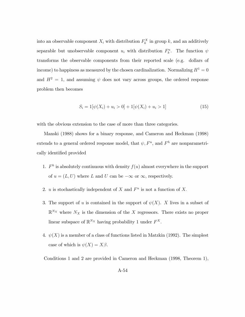
into an observable component Xi with distribution FXk in group k, and an additively

separable but unobservable component ui with distribution F uk . The function

transforms the observable components from their reported scale (e.g. dollars of

income) to happiness as measured by the chosen cardinalization. NormalizingH1 = 0

and H2 = 1, and assuming does not vary across groups, the ordered response

problem then becomes

Si = 1[ (Xi) + ui > 0] + 1[ (Xi) + ui > 1] (15)

with the obvious extension to the case of more than three categories.

Manski (1988) shows for a binary response, and Cameron and Heckman (1998)

extends to a general ordered response model, that ; F u, and F h are nonparametri-

cally identi�ed provided

1. F h is absolutely continuous with density f(u) almost everywhere in the support

of u = (L;U) where L and U can be �1 or 1; respectively.

2. u is stochastically independent of X and F u is not a function of X:

3. The support of u is contained in the support of (X). X lives in a subset of

RNX where NX is the dimension of the X regressors. There exists no proper

linear subspace of RNX having probability 1 under FX :

4. (X) is a member of a class of functions listed in Matzkin (1992). The simplest

case of which is (X) = X�.

Conditions 1 and 2 are provided in Cameron and Heckman (1998, Theorem 1),

A-54

while 3 and 4 are slightly weaker conditions relative to the analogous conditions in

Cameron and Heckman provided by Carneiro, Hansen, and Heckman (2003, Theorem

1) and Cunha, Heckman, and Navarro (2007, Theorem 2).26

References

[1] Adler, Matthew D. 2013. �Happiness Surveys and Public Policy: What�s the

Use?�Duke Law Journal, 62: 1509-1601.

[2] Alesina, Alberto, Rafael Di Tella, and Robert MacCulloch. 2004. �Inequality

and happiness: are Europeans and Americans di¤erent?�Journal of Public Eco-

nomics, 88 (9-10): 2009-2042.

[3] Angeles, Luis. 2010. �Children and Life Satisfaction.� Journal of Happiness

Studies, 11 (4): 523-538.

[4] Black, Dan, Natalia Kolesnikova, Seth Sanders, Lowell Taylor and Mark Wessel.

2009. �A Divergent View on Black-White Earnings Convergence,�unpublished.

[5] Blanch�ower, David G. 2001. �Unemployment, Well-Being, and Wage Curves

in Eastern and Central Europe.� Journal of the Japanese and International

Economies, 15 (4): 364-402.

26For examples of procedures that can estimate the distribution of latent variables without impos-ing strong parametric assumptions, see Hansen, Heckman, and Mullen (2004); Heckman, Stixrud,and Urzua (2006); and Cunha, Heckman, and Schennach (2010). Heckman and Singer (1984)provide an estimator for when Fu is discrete.

A-55

[6] Blanch�ower, David G. 2009. �International Evidence on Well-Being.� in

Krueger, Alan B. (ed.)Measuring the Subjective Well-Being of Nations: National

Accounts of Time Use and Well-Being. University of Chicago Press: Chicago:

155-226.

[7] Blanch�ower, David G. and Andrew J. Oswald. 2004. �Well-Being over time in

Britain and the USA.�Journal of Public Economics, 88 (7-8): 1359-1386.

[8] Blanch�ower, David G. and Andrew J. Oswald. 2008. �Is well-being U-shaped

over the life cycle?�Social Science & Medicine, 66 (8): 1733-1749.

[9] Blanch�ower, David G. and Andrew J. Oswald. 2016. �Antidepressants and

age: A new form of evidence for U-shaped well-being through life.�Journal of

Economic Behavior & Organization, 127: 46-58.

[10] Bond, Timothy N. and Kevin Lang. �The Black-White Education-Scaled Test-

Score Gap in Grades K-7,�Journal of Human Resources. (forthcoming)

[11] Brickman, Phillip, Dan Coates, and Ronnie Jano¤-Bulman. 1978. �LotteryWin-

ners and Accident Victims: Is Happiness Relative?�Journal of Personality and

Social Psychology. 36 (8): 917-927.

[12] Cameron, Stephen V. and James J. Heckman. 1998. �Life Cycle Schooling and

Dynamic Selection Bias: Models and Evidence for Five Cohorts of American

Males.�Journal of Political Economy, 106 (2): 262-333.

[13] Carneiro, Pedro, Karsten T. Hansen, and James J. Heckman. 2003. �Estimat-

ing Distributions of Treatment E¤ects with an Application to the Returns to

A-56

Schooling and Measurement of the E¤ects of Uncertainty on College Choice.�

International Economic Review, 44 (2): 361-421.

[14] Clark, Andrew E. 2003. �Unemployment as a Social Norm: Psychological Evi-

dence from Panel Data.�Journal of Labor Economics, 21 (2): 323-351.

[15] Clark, Andrew E., Sarah Fleche and Claudia Senik. 2014. �The Great Happi-

ness Moderation,� in A.E. Clark and C. Senik, eds., Happiness and Economic

Growth: Lessons from Developing Countries, Oxford: Oxford University Press.

[16] Clark, Andrew E., Sarah Fleche and Claudia Senik. 2016. �Economic Growth

Evens Out Happiness: Evidence from Six Surveys,� Review of Income and

Wealth. 62 (3): 405-419.

[17] Clark, Andrew E., Paul Frijters, and Michael A. Shields. 2008. �Relative Income,

Happiness, and Utility: An Explanation for the Easterlin Paradox and Other

Puzzles.�Journal of Economic Literature, 46 (1): 95-144.

[18] Clark, Andrew E. and Andrew J. Oswald. 1994. �Unhappiness and Unemploy-

ment.�Economic Journal, 104 (424): 648-659.

[19] Cunha, Flavio, James J. Heckman, and Salvador Navarro. 2007. �The Iden-

ti�cation and Economic Content of Ordered Choice Models with Stochastic

Thresholds.�International Economic Review. 48 (4): 1273-1309.

[20] Cunha, Flavio, James J. Heckman, and Susanne M. Schennach. 2010. �Estimat-

ing the Technology of Cognitive and Noncognitive Skill Formation.�Economet-

rica. 78 (3): 883-931.

A-57

[21] Deaton, Angus. 2008. �Income, Health, Wellbeing Around the World: Evidence

from the Gallup World Poll.�Journal of Economic Perspectives, 22 (2): 53-72.

[22] Deaton, Angus and Arthur A. Stone. 2014. �Evaluative and hedonic wellbeing

among those with and without children at home.�Proceedings of the National

Academy of Sciences, 111 (4): 1328-1333.

[23] Dias-Gimenez, Javier, Andy Glover and Jose-Victor Rios-Rull. 2011. �Facts on

the Distribution of Earnings, Income, and Wealth in the United States: 2007

Update.�Federal Reserve Bank of Minneapolis Quarterly Review, 34 (1): 2-31.

[24] Diener, Ed, Carol L. Gohm, Eunkook Suh, and Shigehiro Oishi. 2000. �Similar-

ity of the Relations between Marital Status and Subjective Well-Being across

Cultures.�Journal of Cross-Cultural Psychology, 31 (4): 419-436.

[25] Di Tella, Rafael, Robert J. MacCulloch, and Andrew J. Oswald. 2001. �Prefer-

ences over In�ation and Unemployment: Evidence from Surveys of Happiness.�

American Economic Review, 91 (1): 335-341.

[26] Dutta, Indranil and James Foster, 2013. �Inequality of Happiness in the U.S.:

1972-2010,�Review of Income and Wealth, 59 (3): 393-415.

[27] Easterlin, Richard A. 1973. �Does Money Buy Happiness?�The Public Interest,

30 (3): 3-10.

[28] Easterlin, Richard A. 1974. �Does Economic Growth Improve the Human Lot?�

In Nations and Households in Economic Growth: Essays in Honor of Moses

A-58

Abramovitz, ed. Paul A. David and Melvin W. Reder, 89-125. New York: Aca-

demic Press.

[29] Easterlin, Richard A. 1995. �Will Raising the Incomes of All Increase the Hap-

piness of All?�Journal of Economic Behavior and Organization, 27 (1): 35-47.

[30] Fleurbaey, Marc and Didier Blanchet. 2013. Beyond GDP: Measuring Welfare

and Assessing Sustainability. Oxford University Press: Oxford.

[31] Frijters, Paul and Tony Beatton. 2012. �The mystery of the U-shaped relation-

ship between happiness and age.�Journal of Economic Behavior & Organiza-

tion. 82 (2): 525-542.

[32] Glenn, Norval. 2009. �Is the apparent U-shape of well-being over the life course

a result of inappropriate use of controls? A commentary on Blanch�ower and

Oswald (66:8, 1733-1749).�Social Science & Medicine, 69 (4): 481-485.

[33] Hansen, Karsten T., James J. Heckman, and Kathleen J. Mullen. 2004. �The

E¤ect of Schooling and Ability on Achievement Test Scores.�Journal of Econo-

metrics. 121 (1-2): 39-98.

[34] Heckman, James J. and Burton Singer. �A Method for Minimizing the Impact of

Distributional Assumptions in Econometric Models for Duration Data.�Econo-

metrica, 52 (2): 271-320.

[35] Heckman, James J., Jora Stixrud, and Sergio Urzua. 2006. �The E¤ects of

Cognitive and Noncognitive Abilities on Labor Market Outcomes and Social

Behavior.�Journal of Labor Economics, 24 (3): 411-481.

A-59

[36] Kahneman, Daniel. 2011. Thinking Fast and Slow. New York: Farrar, Strauss

and Giroux, 2011.

[37] Kassenboehmer, Sonja C. and John P. Haisken-DeNew. 2012. �Heresy or en-

lightenment? The well-being age U-shape e¤ect is �at.�Economics Letters, 117:

235-238.

[38] Katz, Lawrence F., Je¤rey R. Kling, and Je¤rey B. Liebman. 2001. �Moving to

Opportunity in Boston: Early Results of a Randomized Mobility Experiment.�

Quarterly Journal of Economics, 116 (2): 607-654.

[39] King, Gary, Christopher J. L. Murray, Joshua A. Salomon and Ajay Tandon.

2004. �Enhancing the Validity and Cross-Cultural Comparability of Measure-

ment in Survey Research.�American Political Science Review, 98 (1): 191-207.

[40] Kling, Je¤rey R., Je¤rey B. Liebman, and Lawrence F. Katz. 2007. �Experi-

mental Analysis of Labor Market E¤ects.�Econometrica, 75 (1): 83-119.

[41] Lucas, Richard E., Andrew E. Clark, Yannis Georgellis, and Ed Diener. 2003.

�Reexamining adaptation and the set point model of happiness: Reactions to

changes in marital status.�Journal of Personality and Social Psychology, 84 (3):

527-539.

[42] Ludwig, Jens, Greg J. Duncan, Lisa A. Gennetian, Lawrence F. Katz, Ronald

C. Kessler, Je¤rey R. Kling, Lisa Sanbonmatsu. 2012. �Neighborhood E¤ects

on the Long-Term Well-Being of Low-Income Adults,�Science, 337: 1505-1510.

A-60

[43] Ludwig, Jens, Greg J. Duncan, Lisa A. Gennetian, Lawrence F. Katz, Ronald C.

Kessler, Je¤rey R. Kling, Lisa Sanbonmatsu. 2013. �Long-Term Neighborhood

E¤ects on Low-Income Families: Evidence fromMoving to Opportunity.�NBER

Working Paper No. 18772.

[44] Le Bon, Olivier and Serge-Daniel Le Bon. 2014. �Age distribution curve in

psychiatric admissions inversely correlates with Life Satisfaction.� Psychiatry

Research. 219 (1): 232-234.

[45] Manski, Charles F. 1988. �Identi�cation of Binary Response Models.�Journal

of the American Statistical Association, 83 (403): 729-738.

[46] Matzkin, Rosa L. 1992. �Nonparametric and Distribution-Free Estimation of

the Binary Threshold Crossing and the Binary Choice Models.�Econometrica,

60(2): 239-270.

[47] Oswald, Andrew J. 2008. �On the curvature of the reporting function from

objective reality to subjective feelings.�Economics Letters, 100 (3): 369-372.

[48] Oswald, Andrew J. and Nattavudh Powdthavee. 2008. �Does happiness adapt?

A longitudinal study of disability with implications for economists and judges.�

Journal of Public Economics. 92 (5-6): 1061-1077.

[49] Rosenbaum, James E. 1995. �Changing the Geography of Opportunity by Ex-

panding Residential Choice: Lessons from the Gautreaux Program.�Housing

Policy Debate, 6 (1): 231-269.

A-61

[50] Ruhm, Christopher. 2000. �Are Recessions Good for Your Health?�Quarterly

Journal of Economics, 115 (1): 617-50.

[51] Smith, Tom W. 1990. Timely Artifacts: A review of measurement variation in

the 1972-1989 GSS. GSS Methodological Report No. 56. Chicago: NORC.

[52] Stack, Steven and J. Ross Eshelman. 1998. �Marital Status and Happiness: A

17-Nation Study.�Journal of Marriage and Family, 60 (2): 527-536.

[53] Stanca, Luca. �Su¤er the little children: Measuring the e¤ects of parenthood on

well-being worldwide.�Journal of Economic Behavior & Organization, 81 (3):

742-750.

[54] Steptoe, Andrew, Angus Deaton, and Arthur A Stone. 2015. �Subjective well-

being, health, and ageing.�Lancet. 385: 640-648.

[55] Stevenson, Betsey and Justin Wolfers. 2008a. �Economic Growth and Subjective

Well-Being: Reassessing the Easterlin Paradox.�Brookings Papers on Economic

Activity, 1-87.

[56] Stevenson, Betsey and Justin Wolfers. 2008b. �Happiness Inequality in the

United States.�Journal of Legal Studies, 37(2): S33-79.

[57] Stevenson, Betsey and Justin Wolfers. 2009. �The Paradox of Declining Female

Happiness.� American Economic Journal: Economic Policy, 1(2): 190-225.

[58] Weiss, Alexander, James E. King, Miho Inoue-Murayama, Tetsuro Matsuzawa,

and Andrew J. Oswald. 2012. �Evidence for a midlife crisis in great apes consis-

A-62

tent with the U-shape in human well-being.�Proceedings of the National Acad-

emy of Sciences, 109 (49): 19949-19952.

[59] Williams, Richard. 2010. �Fitting heterogeneous choice models with oglm.�

Stata Journal, 10 (4): 540-567.

A-63