WP/15/91

The Role of Productivity, Transportation Costs, and Barriers to Intersectoral Mobility in Structural Transformation

by Cem Karayalcin and Mihaela Pintea

© 2015 International Monetary Fund WP/15/91

IMF Working Paper

Research Department and Strategy, Policy, and Review Department

The Role of Productivity, Transportation Costs, and Barriers to Intersectoral Mobility

in Structural Transformation

Prepared by Cem Karayalcin and Mihaela Pintea

Authorized for distribution by Andrew Berg and Catherine Pattillo

March 2015

Abstract

The process of economic development is characterized by substantial reallocations of resources

across sectors. In this paper, we construct a multi-sector model in which there are barriers to the

movement of labor from low-productivity traditional agriculture to modern sectors. With the barrier

in place, we show that improvements in productivity in modern sectors (including agriculture) or

reductions in transportation costs may lead to a rise in agricultural employment and through terms-of-

trade effects may harm subsistence farmers if the traditional subsistence sector is larger than a critical

level. This suggests that policy advice based on the earlier literature needs to be revised. Reducing

barriers to mobility (through reductions in the cost of skill acquisition and institutional changes) and

improving the productivity of subsistence farmers needs to precede policies designed to increase the

productivity of modern sectors or decrease transportation costs.

JEL Classification Numbers: E23; O10; O4; Q10

Keywords: Structural transformation; Subsistence agriculture; multi-sector models;

Economic development; Transportation costs

Author’s E-Mail Address : karayalc@fiu.edu; pinteam@fiu.edu

1. We would like to thank Adrian Peralta-Alva, Andrew Berg, Gerhard Glomm, Donald Larson, PrakashLoungani, Catherine Pattillo, Chris Papageorgiou, Diego Restuccia, Francis Teal, Luis-Felipe Zanna and seminar participants at the research department of the IMF, as well as conference participants at the Fall 2014 Midwest Macro Meetings for useful comments and suggestions. Portions of this paper were written while Pintea was on leave at the IMF. This working paper is part of a research project on macroeconomic policy in low-

income countries supported by the U.K.'s Department for International Development. The views expressed in this Working Paper are those of the authors and do not necessarily represent those of the IMF, IMF policy, or of DFID.

IMF Working Papers describe research in progress by the author(s) and are published to elicit

comments and to encourage debate. The views expressed in IMF Working Papers are those of the

author(s) and do not necessarily represent the views of the IMF, its Executive Board, or IMF management.

3

Content Page

1. Introduction……………………………………………………………………… 4

2. The Model ……………………………………………………………………….. 7

2.1 Firms ………………………..………………………………..…………. 7

2.2 Households …………………….……………………………..…………. 8

2.3 Market Clearing …………………..…………………………..………… 10

2.4 Equilibrium ……………………………………………………....…….. 10

2.5 Productivity Shocks…………………………………………… ………. 11

2.5.1 In the Manufacturing Sector ……………..……………... 11

2.5.2 In Modern Agriculture …………………..……………… 12

2.5.3 In Subsistence Agriculture ……………..……………….. 13

2.6 Transportation Costs of Intermediate Inputs……………………………. 14

3 Quantitative Analysis……………………………………………..……… ………… 14

3.1 Changes in Productivity and Transportation Costs …………………….. 16

4 Conclusion……. ……………………………………………………………………. 20

TABLES

1. Base Parameters…………………………………………………………… ……. 15

2. Base Equilibria An = Am = 2.8 ……………………………………………… ……. 15

3. Base Equilibria An = Am = 4.5 ……………………………………………… ……. 16

4. Productivity Shocks ..……………………………………………………… ……. 17

5. Productivity Shocks (An = Am = 2.8)………………………………………… ……. 27

6. Productivity Stocks (An = Am = 4.5) ………………………………………… ……. 28

FIGURES

1. Increase in the Number of Skilled Workers…...……………………….………… 29

2. Increase in Manufacturing Productivity ……………… ………………………… 29

3. Increase in Productivity of Modern Agriculture …… ………………………….. 30

4. Decrease in the Cost of Transportation …….……………………. ………….…. 30

APPENDIX .…………………….………………………………………….………… 23

REFERENCES …………………………………………………………………………... 21

4

1. Introduction

In many developing countries, employment in the agriculture sector is very high relative to that in

the developed countries. Globally, the poorest 5% of the countries have about 86% of their labor force

in agriculture, whereas the richest 5% have less than 5%. In the process of development, economies

experienced significant movements of labor from agriculture into modern sectors.

The notion that economic growth and development has been associated with significant move-

ments of labor out of agriculture and into manufacturing and services (structural transformation)

has been put forward starting with Clark (1940), Kuznets (1966), Rostow (1959) and Chenery and

Syrquin (1975). More recently economists have focused on structural transformation in the context

of multi-sector models in order to present a more nuanced explanation of differences in productiv-

ity and growth rates across countries. This literature has emphasized, on the one hand, differences

in productivity across agricultural and non-agricultural sectors1 and, on the other hand, barriers

to structural transformation that include costs of transportation, of skill acquisition, and cultural

factors. In this paper, we develop a general equilibrium model that incorporates both productivity

differences and some empirically prominent barriers to the transformation of the economy from one

where subsistence agriculture is dominant to one where modern sectors play a more significant role.

In what follows, we construct a three-sector model with a traditional subsistence agriculture,

modern agriculture, and a non-agricultural sector (manufacturing and/or services). Agricultural

goods are produced in the rural sector, whereas manufacturing and services are produced in the

urban areas. Our setup differs from existing ones along a number of dimensions. Perhaps most im-

portantly, we bring together two strands of the recent literature. The first of these emphasizes the

role played by barriers to goods mobility, such as transportation costs for the movement of labor out

of agriculture. Herrendorf et al. (2012) study the effect of the construction of railroads in the US

during 1840-1860, and find that the associated reduction in transportation costs lead to settlement

of the most fertile land in the Midwest, and a reduction in the agricultural labor force. Adamopou-

los (2011) shows that transportation costs can lead to low aggregate output per worker, by reducing

productivity within sectors and distorting allocation of resources across locations and between sec-

tors. He analyzes the effect of cross country transportation cost disparities and finds that improve-

ments in transportation productivity would have an asymmetric result on the poor and developed

countries, with the former gaining more. Gollin and Rogerson (2014) allow for heterogeneity in agri-

culture through differences in the costs of transportation. They carry out some numerical exercises

matching the parameters of their model to a typical sub-Saharan economy and find that transporta-

tion costs are quantitatively important in terms of both allocations and welfare.The second strand,

exemplified by Caselli and Coleman (2001) and Hayashi and Prescott (2008), focuses on barriers to

1 Restuccia, Yang and Zhu (2008) look at labor productivity differences in both agriculture and non-agriculture betweenthe richest 5% of the countries and poorest 5%. They report that GDP per worker differences in agriculture is a factor of 78,whereas in non-agriculture it is a factor of 5. Based on these productivity differences, McMilan and Rodrik (2011) argue that asmuch as a fifth of the productivity gap between developing and advanced countries would be eliminated if the inter-sectoraldistribution of employment in the developing countries matched that in the developed countries. Gollin, Lagakos and Waugh(2014) report that in countries in the lowest quartile of income distribution, the value added per worker is about 5.6 higher innon-agriculture than in agriculture, and this factor drops to 2 for the upper quartile.

5

labor mobility that keep agricultural employment relatively high for extended periods of time in the

process of development. These barriers may take a number of different forms. Caselli and Coleman

(2001) emphasize the costly acquisition of skills as the barrier that impedes the movement of labor

from agriculture into non-agricultural employment. Hayashi and Prescott (2008), on the other hand,

argue that both the cultural values of the Japanese extended family and the institutions of prewar

Japan acted as barriers to the movement of labor out of agriculture in the 1885-1940 period2. In the

rest of the paper, we adopt the specific barrier suggested by Caselli and Coleman (2001) and sup-

pose that labor employed in subsistence agriculture is unskilled, whereas both modern agriculture

and manufactures employ skilled labor with no possibilities of substitution anywhere between these

two types of labor. We also assume that the cost of skill acquisition is too high for unskilled work-

ers. However, this specific barrier could be interpreted in any number of ways and as long as there

exists some barrier to the mobility of labor between the traditional and modern sectors, our conclu-

sions will remain valid. In addition our model incorporates productivity differences across sectors

as well as transportation costs. We model productivity differences by taking the idea that through-

out the development process modern and traditional technologies coexist seriously and incorporate

two agricultural sectors that produce a single agricultural good using a traditional technology (in

the subsistence sector) and a modern technology 3. As for transportation costs, our model incorpo-

rates three types: the ones involved in transporting manufactures to rural areas as both a consump-

tion good and an intermediate input in the production in modern agriculture, and those involved in

transporting the agricultural good from the rural to the urban areas.

Our model produces a number of novel insights with regard to the interaction of different sectors,

technologies and barriers in the process of structural transformation. One of the most important of

these insights concerns the effects of productivity improvements in modern agriculture. In a stan-

dard model of the type used in the existing literature, this improvement would lead to agriculture

shedding labor and manufactures expanding employment and output. This is still the case in our

model if the initial subsistence agriculture employment and output are lower than a critical value.

However, if the initial size of the subsistence agriculture is large enough, the modern agriculture sec-

tor expands in response to a technological shock that makes it more productive. The intuitive reason

for this hinges upon the changes in terms of trade faced by both agricultural sectors that produce

the same good as the size of subsistence agriculture crucially affects the relative demand changes

for both the agricultural and manufacturing goods. We also show that the interactions between the

barrier to labor mobility and the simultaneous use of traditional and modern technologies in agri-

culture give rise to welfare reductions for subsistence farmers who get hurt by the deterioration of

their terms of trade when modern agriculture becomes more productive. Similar perverse welfare

results arise in cases when there are reductions in transportation costs that lower the terms of trade

subsistence farmers face. These results are established analytically in our setup.

2O’Brien (1996) argues that much of the explanation for the persistence of a comparatively large subsistence agriculturesector in France (as opposed to England) prior to the twentieth century lies in the cultural and institutional factors that kepta large fraction of the labor force in rural areas of France.

3Gollin, Parente and Rogerson (2004) also develop a growth model with agricultural sector where agricultural and non-agricultural output can be produced with different technologies contemporaneously, in their case however they focus onmarket and home production.

6

We then turn to counterfactual numerical exercises by calibrating our model as far as possible

to match the stylized features of a sub-Saharan African economy. Here we are interested in the

magnitude of the differential effects of changes in productivity and transportation costs taken either

separately or grouped together. Our focus is the consequences of these changes on the economy’s

potential structural transformation (as measured by the allocation of resources across sectors) and

on the changes in welfare of different groups in society. We find that improvements in the produc-

tivity of modern agriculture have significant negative welfare consequences on subsistence farmers

through terms of trade deteriorations, but benefit workers in the modern sectors. As mentioned

before, in contrast to the findings in the existing literature, whether the modern agriculture sector

expands or contracts in response depends on the initial size of subsistence agriculture. Improve-

ments in manufacturing productivity improve the welfare of all workers (with subsistence farmers

benefiting from a terms of trade improvement), yet their effect on the allocation of resources across

sectors and the magnitude of changes in welfare depend again on the initial size of the subsistence

agriculture sector. In terms of the direction and magnitude of structural transformation improve-

ments in the productivity of the subsistence sector appear to be the most important as they lead to

the most substantial reallocations of skilled labor away from (modern) agriculture to manufactures.

Not surprisingly, subsistence farmers gain the most in terms of welfare when it is their productivity

that rises. Reductions in transportation costs have comparatively small effects on the allocation of

resources and welfare either taken by themselves or together with other changes. Finally, lowering

the barrier to the intersectoral mobility of labor in the form of a reduction in the cost of skill acqui-

sition that enables some unskilled to become skilled reduces the share of agricultural output in total

output while reducing the labor force engaged in agriculture.

Our model is most closely related to Gollin and Rogerson (2014). We differ most importantly from

Gollin and Rogerson (2014) in that we allow for barriers to the mobility of labor between the subsis-

tence sector and the modern sectors. Together with heterogeneity in agriculture through differences

in production techniques, including the type of resources employed, our model yields a richer set of

results concerning the effects of changes in (both agricultural and manufacturing) productivity and

transportation costs. Thus, whether improvements in, say the productivity of modern agriculture,

result in a reallocation of labor away from it depends crucially on the size of the subsistence agri-

cultural sector that is modeled to be less productive. Our richer set of results include those of Gollin

and Rogerson (2014) as a subset: the smaller is the size of subsistence agriculture the more likely it is

for improvements in productivity of modern agriculture to reduce the latter’s share of employment.

Further, we show that such improvements reduce the welfare of subsistence farmers through their

negative impact on the terms of trade such farmers face, and may reduce the overall welfare as well.

What these results suggest, in contrast to the existing literature, is that in the poorest developing

countries with large subsistence agriculture sectors, policy needs to follow a sequence. Measures

that reduce barriers to labor mobility from subsistence farming to modern sectors and that help

raise the productivity of subsistence farmers need to precede implementation of policies that are

designed to increase productivity in modern sectors or decrease transportation costs.

The paper proceeds as follows. Section 2 describes the model. Section 3 presents the calibration

and quantitative evaluation. Section 4 concludes.

7

2. The Model

2.1. Firms

A typical assumption made in the literature on structural transformation is that agricultural sector is

the traditional one and manufacturing and services are the modern ones without taking into consid-

eration the heterogeneity of production technologies in the economy. In contrast, we assume that

even though the non-agriculture good is produced only with modern technology, there are two avail-

able technologies for producing the agricultural good: a subsistence/traditional and a modern one.4

Thus modern technology could be used in either modern agriculture or non-agriculture sector, and

in what follows, we suppose that education is a barrier to adopting modern technologies. Firms take

the technology that they can use as given. Farms in the subsistence sector use unskilled labor as

the only factor of production. Letting population be equal to a mass n and educated workers equal

to a mass ne yields the unskilled workers to be equal to n − ne. Assuming a constant input-output

coefficient of 1/Au, the output, Y Au , of “food” by the subsistence agriculture sector is then given by:

Yu = Au (n− ne) (1)

Competitive firms produce food in the modern agriculture sector by combining intermediate inputs

z and a fraction θ of skilled labor in a CRS Cobb-Douglas form:

Yn = An(θne)βz1−β (2)

Intermediate inputs are produced by competitive firms in the manufacturing sector which operate

in the urban area and are subject to iceberg transportation costs η, such that farms in modern agri-

culture pay effectively p(1 + η), where p is the relative price of manufactured good in terms of food.

Firms in modern agriculture choose the optimal amount of intermediate inputs and labor used

in modern agriculture to maximize profits Yn − wnnn − p(1 + η)z (where nn := θne). The solution of

this problem yields the following first-order conditions

p(1 + η) = (1− β)Ank−β (3)

wn = βAnk1−β, (4)

where we define the capital-labor ratio k as k := z/(θne).

4One could argue that heterogeneous technologies exist in both the agriculture and non-agriculture sectors and focusingon the different technologies just in the agriculture sector may be misleading. However, we focus on the heterogeneity inthe agriculture sector for two reasons. First, as Eberhardt and Teal (2012) show the heterogeneity of production functions(measured by the capital coefficients) in agriculture is much wider than that in the manufacturing sector. Secondly, thisheterogeneity is quite substantial in the poorest developing countries on which this paper focuses.

8

Note that the total amount of labor in agriculture is na = n− ne + θne.

The only input of production in the manufactures sector is skilled labor:

Ym = Amnm (5)

where subscripts m denote manufactures and nm = (1 − θ)ne. Firms in manufacturing choose the

optimal amount of skilled labor to maximize profits pYm−wmnm. The solution of this problem yields

the following first order condition: wm = pAm.

We also impose the condition that MPL in modern sector is always higher than in traditional

agriculture, with the result that skilled workers will choose to work only in the modern sectors. We

also note that wages in the modern sector do not have to be necessarily equal.

2.2. Households

All households consume food and manufactured goods according to the same non-homothetic util-

ity function, and differ only in the budget constraint that they face. Their preferences are given by

u(cAj , cMj ) = αln(cAj − cA) + lncMj (6)

where cA > 0 denotes the subsistence level of food consumption and α > 0 is the relative weight of

food in preferences. Finally, cAj denotes individual consumption of food and cMj denotes individual

consumption of manufacturing good (j = m,u, n). This formulation yields an income elasticity of

food demand that is below one. Let m, n, u represent households that live in urban areas and work

in the manufacturing sector, that live in rural areas and work in the modern agriculture sector, and

that live in rural areas and work in subsistence agriculture, respectively.

Both type of workers supply their labor endowment inelastically.

Consumers in rural areas pay a price inclusive of transportation costs, η1, for the manufactured

goods, and receive a wage equal to their marginal product of labor:

wi = cAi + p(1 + η1)cMi (7)

where i = u, n.

9

Consumers living in the urban areas receive a wage from working in the manufacturing sector

and the price they pay for food includes the cost, η2, of transporting it from the rural areas:

wm = cAm(1 + η2) + pcMm (8)

We also assume that the level of agricultural productivity is high enough so that our economy

operates above the subsistence level of food (i.e. Au ≥ cA) .

Households maximize (6) subject to their respective budget constraints 7 and 8. The optimality

conditions imply that households equate the marginal rate of substitution between the two con-

sumption goods to the relative price, incorporating transportation costs such that

cAi = cA + αp(1 + η1)cMi (9)

where i = u, n and

cAm = cA +αpcMm1 + η2

(10)

Using the first order conditions and budget constraints for the households, and the profit max-

imization conditions for the firms in the modern sectors we can derive analytically individual con-

sumption levels for both unskilled and skilled workers as function of their wages.

cAu =cA + αAu

1 + α, cMu =

Au − cAp (1 + α) (1 + η1)

(11a)

cAn =cA + αwn

1 + α, cMn =

wn − cAp (1 + α) (1 + η1)

(11b)

cAm =cA (1 + η2) + αwm

(1 + α) (1 + η2), cMm =

wm − (1 + η2) cAp (1 + α)

(11c)

10

2.3. Market clearing

Aggregating across sectors and assuming, by Walras’ law, that excess demand for food, EDA, equals

zero in equilibrium yields:

EDA := DA − SA = (n− ne)cAu + θnec

An + (1− θ)nec

Am(1 + η2)− (Yu + Yn) = 0. (12)

Substituting equation (3) into (12) we can express the excess demand for food,EDA, as a function of

k, θ, and the parameters

EDA := ψ(θ, k;An, Am, Au, η, η1, η2, n, ne, cA), (13)

with ψi > 0 i ∈ 4, 8, 10, 11, ψi < 0 i ∈ 1, 2, 5, 6, 9, ψi ≶ 0 i = 3, ψi = 0 i = 7, where DA and SA

denote the demand for and supply of food production and

YM = (1 + η1)[

(n− ne)cMu + θnec

Mn

]

+ (1− θ)necMm + z(1 + η) (14)

So that aggregate output of food, Y A(=SA) can be expressed as

Y A = ncA + η2 (1− θ)necA + αp[YM − z(1 + η)]. (15)

Since there are no impediments to the movement of labor across the two modern sectors, in

utility terms skilled workers will receive the same pay-off in these two sectors:

Unm := Un − Um = (1 + α)

lnwn − cA

wm − (1 + η2)cA

+ α ln(1 + η2)− ln(1 + η) = 0 (16)

where Ui (i = n,m) denotes the utility pay-off to skilled labor working in sector i and using (3) we

have

Unm = ϕ(θ, k;An, Am, Au, η, η1, η2, n, ne, cA). (17)

with ϕi > 0 i ∈ 2, 6, 8, 11 ϕi < 0 i ∈ 3, 4, 7, ϕi = 0 i ∈ 1, 5, 9, 10.All the partial derivatives, ψi

and ϕi are derived explicitly in the Appendix.

2.4. Equilibrium

An equilibrium for this economy, given transportation costs (η, η1, η2), sectoral productivities (An, Am, Au),

distribution of skill in the population (n, ne), and subsistence level of consumption for the agricul-

tural good cAis characterized by the relative price of manufactured good, capital-labor ratio, as well

11

as the fraction of skilled labor employed in modern agriculture sector (p, k, θ) together with wages

(wn,wm), and allocations of consumption for each type of households that solve their respective con-

strained optimization problem and clear markets.

More precisely, the two equations (3) and (16) jointly solve for p and k. Given the solution for

k, equation (12) can then be used to solve for θ. Equation (4) and wm = pAm then solve for wages,

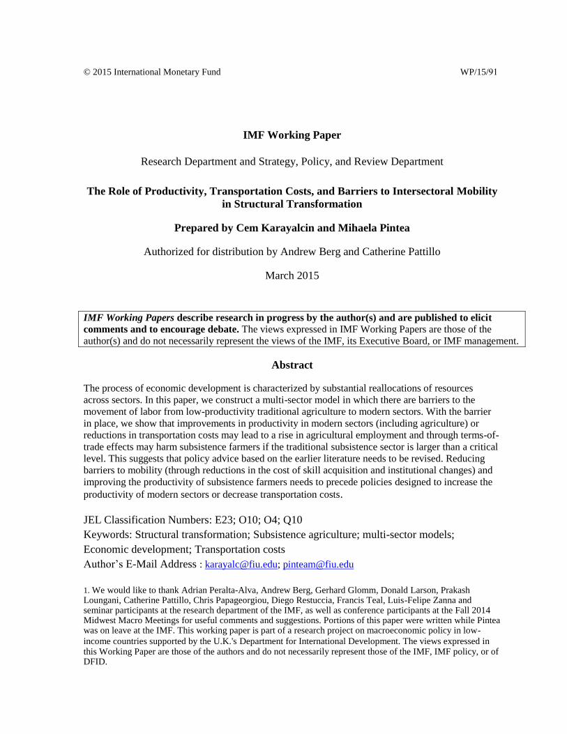
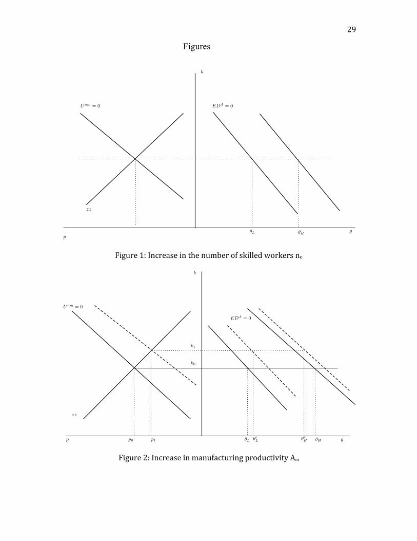
while (11a)-(11c) do so for the consumption levels and (6) for utilities. It is helpful to use Figure 1 to

visualize the solution of the model. The left-hand side panel in the figure displays the determination

of k and p. The curve zz depicting the equation (3) slopes downward as an increase in the relative

price of manufactures, p, reduces the demand for manufactures as an input and lowers k = z/(θne).

The curve labeled Unm = 0 slopes upward as a rise in p increases wm and, thus the utility pay-off

to working in manufactures. Free mobility of labor would then lead to skilled workers moving to

the manufacturing sector, reducing θ and, thus, increasing k. As (3) and (16) depend only on the two

endogenous variables p and k, the left-hand panel of Figure 1 determines these two variables. On the

right-hand panel, the curve EDA = 0 depicting equation (12) is drawn downward sloping as excess

demand for food is decreasing in both k and θ.

As it will play an important role later on in our analysis of productivity shocks, it is useful to

employ Figure 1 to visualize the effects of an increase in the number of skilled workers, ne. First, note

that the change in ne does not affect either k or p (see equations (3) and (16)). It does however, reduce

the supply of food produced by subsistence farmers and increase its demand by raising the number

of skilled workers who receive relatively higher wages. The excess demand these changes generate is

eliminated by an increase in the number of skilled workers employed by modern agriculture. In the

figure, this is depicted by the rightward shift of the ED = 0Acurve and the rise in θ.

2.5. Productivity shocks

We now turn to a discussion of some counterfactual experiments starting with productivity shocks

in the three sectors of the economy.

2.5.1. In the Manufacturing Sector

The first productivity shock we consider is an increase in the productivity Am of the manufacturing

sector. The main result we obtain is summarized in the following Lemma. All the proofs are in the

Appendix.

Lemma 1. A rise in the productivity,Am, of the manufacturing sector reduces (increases) employ-

ment in manufactures (agriculture) if initially subsistence farmers can meet the subsistence food

needs of the economy.

12

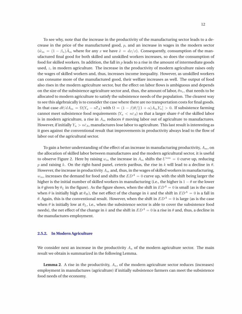
To see why, note that the increase in the productivity of the manufacturing sector leads to a de-

crease in the price of the manufactured good, p, and an increase in wages in the modern sector

(wm = (1 − βn)Am where for any x we have x = dx/x). Consequently, consumption of the man-

ufactured final good for both skilled and unskilled workers increases, so does the consumption of

food for skilled workers. In addition, the fall in p leads to a rise in the amount of intermediate goods

used, z, in modern agriculture. The increase in the productivity of modern agriculture raises only

the wages of skilled workers and, thus, increases income inequality. However, as unskilled workers

can consume more of the manufactured good, their welfare increases as well. The output of food

also rises in the modern agriculture sector, but the effect on labor flows is ambiguous and depends

on the size of the subsistence agriculture sector and, thus, the amount of labor, θne, that needs to be

allocated to modern agriculture to satisfy the subsistence needs of the population. The clearest way

to see this algebraically is to consider the case where there are no transportation costs for final goods.

In that case dθ/dAm = Ω(Yu − ncA) with Ω = (1 − β)θ/[(1 + α)AmYn] > 0. If subsistence farming

cannot meet subsistence food requirements (Yu < ncA) so that a larger share θ of the skilled labor

is in modern agriculture, a rise in Am reduces θ moving labor out of agriculture to manufactures.

However, if initially Yu > ncA, manufactures lose labor to agriculture. This last result is interesting as

it goes against the conventional result that improvements in productivity always lead to the flow of

labor out of the agricultural sector.

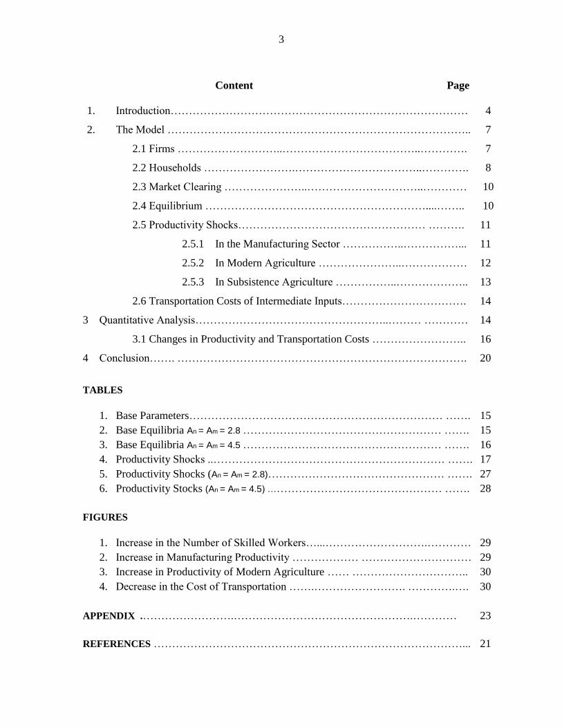
To gain a better understanding of the effect of an increase in manufacturing productivity,Am, on

the allocation of skilled labor between manufactures and the modern agricultural sector, it is useful

to observe Figure 2. Here by raising wm the increase in Am shifts the Unm = 0 curve up, reducing

p and raising k. On the right-hand panel, ceteris paribus, the rise in k will lead to a decline in θ.

However, the increase in productivityAm and, thus, in the wages of skilled workers in manufacturing,

wm, increases the demand for food and shifts the EDA = 0 curve up, with the shift being larger the

higher is the initial number of skilled workers in manufacturing (i.e., the higher is 1 − θ or the lower

is θ given by θL in the figure). As the figure shows, when the shift in EDA = 0 is small (as is the case

when θ is initially high at θH), the net effect of the change in k and the shift in EDA = 0 is a fall in

θ. Again, this is the conventional result. However, when the shift in EDA = 0 is large (as is the case

when θ is initially low at θL, i.e., when the subsistence sector is able to cover the subsistence food

needs), the net effect of the change in k and the shift in EDA = 0 is a rise in θ and, thus, a decline in

the manufactures employment.

2.5.2. In Modern Agriculture

We consider next an increase in the productivity An of the modern agriculture sector. The main

result we obtain is summarized in the following Lemma.

Lemma 2. A rise in the productivity, An, of the modern agriculture sector reduces (increases)

employment in manufactures (agriculture) if initially subsistence farmers can meet the subsistence

food needs of the economy.

13

To see why, note that the increase in the productivity of the modern agriculture sector leads to an

increase in the supply of food, a decline in its relative price, and, thus, a rise in the relative price of

manufactured good, p, and increase in the wages of skilled workers who are employed solely in the

modern sectors. As a result, skilled workers are able to consume both more agriculture and man-

ufactured goods. As the increase in productivity of modern agriculture has no effect on the wages

of unskilled workers, it increases income inequality. Consumption of the manufactured good de-

creases for unskilled workers, reducing their welfare. Production of food increases in the modern

agriculture sector. However, the effect on labor flows out of agriculture and the amount of interme-

diate inputs used in modern agriculture depends as before on the size of subsistence agriculture. To

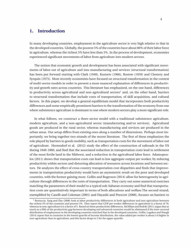
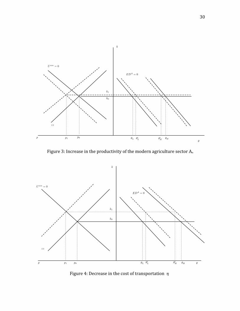
see the effects of the increase in An on θ and k, it is useful to refer to Figure 3, where two initial labor

allocations are indicated as above by θL and θH . The rise in An shifts the zz curve upwards and the

Unm = 0 curve downwards, the net effect being a rise in both k and p. Ceteris paribus, this would

lead to an outflow of skilled labor from modern agriculture to manufactures. However, the rise in An

also leads to a shift of the EDA = 0 curve. Given θ, whether excess demand for food rises or falls

depends on the initial size of the subsistence agriculture sector. If it is small so that we have θH , the

EDA = 0 curve shifts to the left, θ falls and the manufacturing sector expands. This is the case em-

phasized by the existing literature which typically assumes away subsistence agriculture. However,

if subsistence farming is large enough initially with labor allocation given by θL, the improvement in

the productivity, An, of modern agriculture leads to a rightward shift of the EDA = 0 curve, with the

result that θ rises and the manufacturing sector shrinks.

2.5.3. In Subsistence Agriculture

We next turn to the analysis of an increase in the productivity, Au, of the subsistence agriculture

sector. The main result we obtain is summarized in the following Lemma.

Lemma 3. A rise in the productivity,Au, of the subsistence agriculture sector increases (reduces)

employment in manufactures (agriculture).

The mechanism behind this result is straightforward to see: A rise in the productivity, Au, of the

subsistence agriculture, raises the quantity of food produced and increases the incomes of the farm-

ers there, leading to higher levels of consumption of both food and manufactures. Given that the

income elasticity of food demand is below one, demand for food produced in modern agriculture

decreases, such that skilled labor moves away from the modern agriculture sector to manufactures.

The decline in the amount of labor in the former reduces the marginal productivity of the intermedi-

ate input and its use and leads to a decrease in the price of manufactures. The increase in the supply

of food coupled with the higher demand for non-agricultural final good due to increase income of

subsistence workers raises the relative price, p, of the latter. The net effect of these changes is an

unchanged p, higher wages in the subsistence sector, and unchanged wages and consumption levels

for skilled workers.

14

2.6. Transportation costs of intermediate inputs

Finally, we study a decrease in the cost, η, of transporting the intermediate inputs to modern agri-

culture. Our main result is as follows.

Lemma 4. A decrease in the cost, η , of transporting the intermediate inputs to modern agricul-

ture reduces (increases) employment in manufactures (agriculture) if initially subsistence farmers

can meet the subsistence food needs of the economy.

A reasoning similar to our previous results holds here. The decrease in η reduces the cost of pro-

ducing food in the modern agriculture sector and raises the relative price, p, of manufactured goods,

as well as leading to a rise of wages in the modern sector. Consumption of both agricultural and

non-agricultural goods increases for skilled workers, whose welfare improves. As the terms of trade

they face deteriorates with the rise in p, consumption of the final manufactured good and welfare

decreases for unskilled workers. The effect of the fall of η on labor flows out of agriculture, the over-

all amount of intermediate inputs designed to be used in modern agriculture, as well as the total

production of manufactured goods depends on the size of subsistence agriculture relative to the

subsistence food needs of the population.

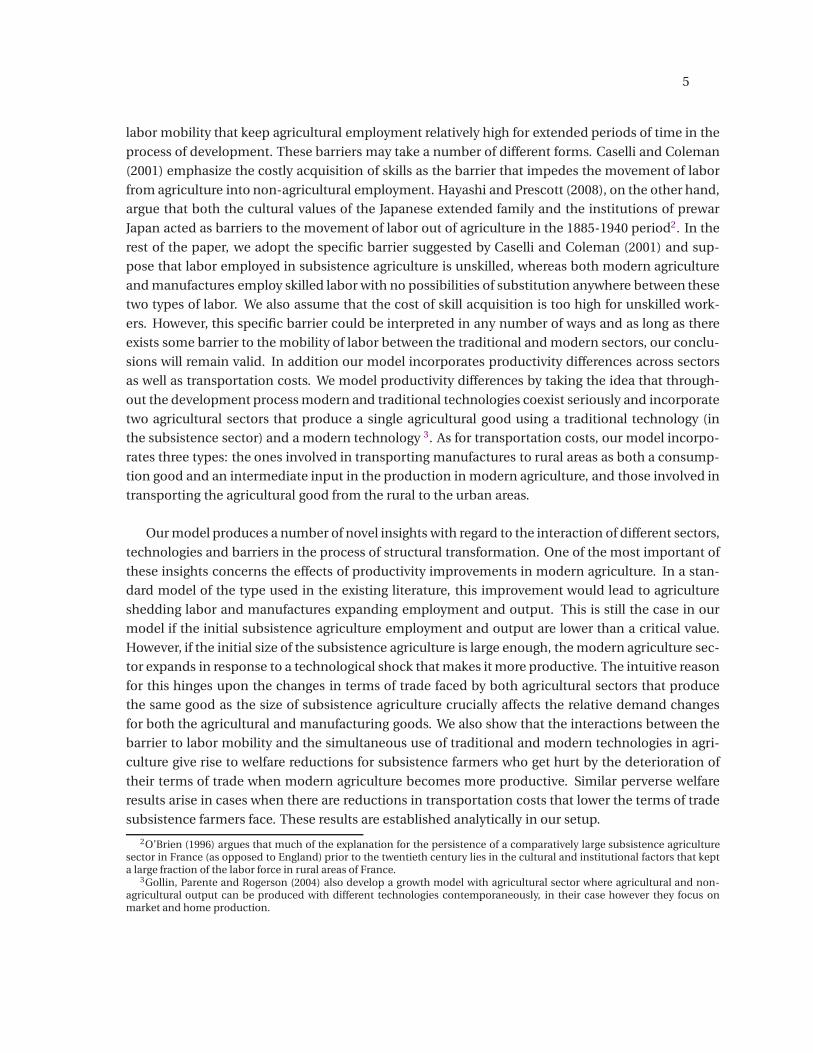
Figure 4 shows the effects of the decrease of η on the allocation of skilled labor. Here the decrease

in costs in modern agriculture leads to an upward shift of the zz curve. The increase in kwould ceteris

paribus reduce θ, however, the fall in η increases excess demand for food and shifts the EDA = 0

rightward. As before, if initially the subsistence sector is relatively small (θ is relatively high at θH)

the shift in EDA = 0 is small and and the agriculture sector shrinks as in the existing literature.

Otherwise, the shift inEDA = 0 (with an initial θ at θL) is larger, with the result that θ rises, and, thus,

the manufacturing sector loses workers and shrinks.

3. Quantitative analysis

In this section we complement the analytical results obtained above with a quantitative analysis de-

signed to illustrate the relative magnitudes of the effects of the counterfactual experiments described

previously. We calibrate our model to be consistent with the most salient features of sub-Saharan

economies relevant for our purposes. This numerical analysis also allows us consider the relative

welfare consequences of changes in productivity, transportation costs, and the share of skilled work-

ers in the labor force. We also incorporate the transportation costs of the final goods.

We normalize the size of the population n, to be equal to one. We set labor income share in the

modern agriculture sector β = 0.4, implying a share for intermediate inputs of 1 − β = 0.6. The

preference parameter for food is α = 0.2. We normalize Au = 1 and set cA = 0.6. Since our results

depend critically on whether initially the subsistence agriculture sector produces enough to meet

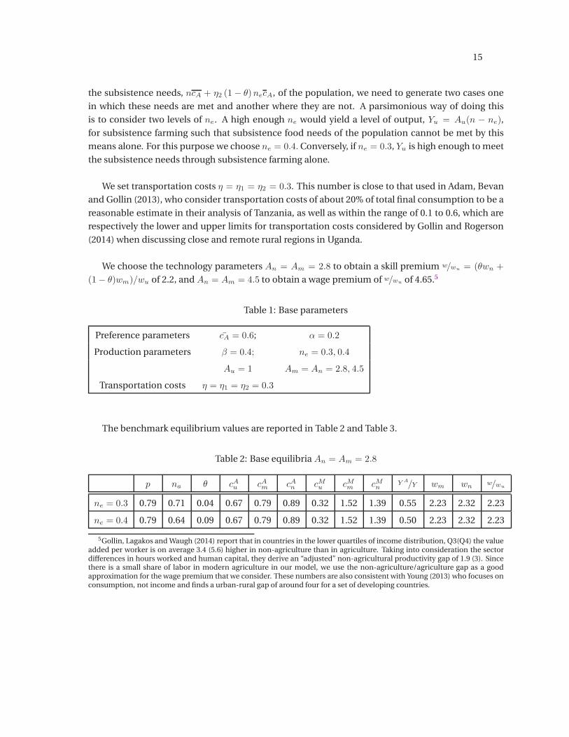
15

the subsistence needs, ncA + η2 (1− θ)necA, of the population, we need to generate two cases one

in which these needs are met and another where they are not. A parsimonious way of doing this

is to consider two levels of ne. A high enough ne would yield a level of output, Yu = Au(n − ne),

for subsistence farming such that subsistence food needs of the population cannot be met by this

means alone. For this purpose we choose ne = 0.4.Conversely, if ne = 0.3, Yu is high enough to meet

the subsistence needs through subsistence farming alone.

We set transportation costs η = η1 = η2 = 0.3. This number is close to that used in Adam, Bevan

and Gollin (2013), who consider transportation costs of about 20% of total final consumption to be a

reasonable estimate in their analysis of Tanzania, as well as within the range of 0.1 to 0.6, which are

respectively the lower and upper limits for transportation costs considered by Gollin and Rogerson

(2014) when discussing close and remote rural regions in Uganda.

We choose the technology parameters An = Am = 2.8 to obtain a skill premium w/wu = (θwn +

(1− θ)wm)/wu of 2.2, and An = Am = 4.5 to obtain a wage premium of w/wu of 4.65.5

Table 1: Base parameters

Preference parameters cA = 0.6; α = 0.2

Production parameters β = 0.4; ne = 0.3, 0.4

Au = 1 Am = An = 2.8, 4.5

Transportation costs η = η1 = η2 = 0.3

The benchmark equilibrium values are reported in Table 2 and Table 3.

Table 2: Base equilibria An = Am = 2.8

p na θ cAu cAm cAn cMu cMm cMn Y A/Y wm wn w/wu

ne = 0.3 0.79 0.71 0.04 0.67 0.79 0.89 0.32 1.52 1.39 0.55 2.23 2.32 2.23

ne = 0.4 0.79 0.64 0.09 0.67 0.79 0.89 0.32 1.52 1.39 0.50 2.23 2.32 2.23

5Gollin, Lagakos and Waugh (2014) report that in countries in the lower quartiles of income distribution, Q3(Q4) the valueadded per worker is on average 3.4 (5.6) higher in non-agriculture than in agriculture. Taking into consideration the sectordifferences in hours worked and human capital, they derive an “adjusted” non-agricultural productivity gap of 1.9 (3). Sincethere is a small share of labor in modern agriculture in our model, we use the non-agriculture/agriculture gap as a goodapproximation for the wage premium that we consider. These numbers are also consistent with Young (2013) who focuses onconsumption, not income and finds a urban-rural gap of around four for a set of developing countries.

16

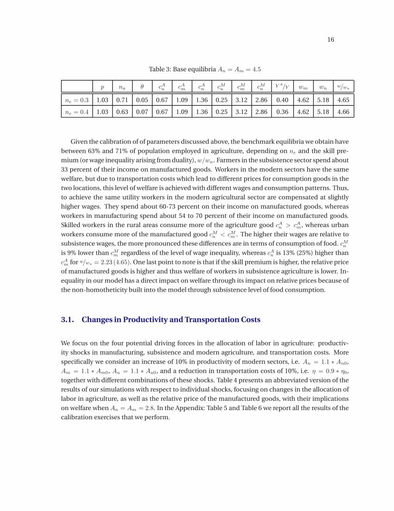
Table 3: Base equilibria An = Am = 4.5

p na θ cAu cAm cAn cMu cMm cMn Y A/Y wm wn w/wu

ne = 0.3 1.03 0.71 0.05 0.67 1.09 1.36 0.25 3.12 2.86 0.40 4.62 5.18 4.65

ne = 0.4 1.03 0.63 0.07 0.67 1.09 1.36 0.25 3.12 2.86 0.36 4.62 5.18 4.66

Given the calibration of of parameters discussed above, the benchmark equilibria we obtain have

between 63% and 71% of population employed in agriculture, depending on ne and the skill pre-

mium (or wage inequality arising from duality),w/wu. Farmers in the subsistence sector spend about

33 percent of their income on manufactured goods. Workers in the modern sectors have the same

welfare, but due to transportation costs which lead to different prices for consumption goods in the

two locations, this level of welfare is achieved with different wages and consumption patterns. Thus,

to achieve the same utility workers in the modern agricultural sector are compensated at slightly

higher wages. They spend about 60-73 percent on their income on manufactured goods, whereas

workers in manufacturing spend about 54 to 70 percent of their income on manufactured goods.

Skilled workers in the rural areas consume more of the agriculture good cAn > cAm, whereas urban

workers consume more of the manufactured good cMn < cMm . The higher their wages are relative to

subsistence wages, the more pronounced these differences are in terms of consumption of food. cMnis 9% lower than cMm regardless of the level of wage inequality, whereas cAn is 13% (25%) higher than

cAm for w/wu = 2.23 (4.65). One last point to note is that if the skill premium is higher, the relative price

of manufactured goods is higher and thus welfare of workers in subsistence agriculture is lower. In-

equality in our model has a direct impact on welfare through its impact on relative prices because of

the non-homotheticity built into the model through subsistence level of food consumption.

3.1. Changes in Productivity and Transportation Costs

We focus on the four potential driving forces in the allocation of labor in agriculture: productiv-

ity shocks in manufacturing, subsistence and modern agriculture, and transportation costs. More

specifically we consider an increase of 10% in productivity of modern sectors, i.e. An = 1.1 ∗ An0,

Am = 1.1 ∗ Am0, Au = 1.1 ∗ Au0, and a reduction in transportation costs of 10%, i.e. η = 0.9 ∗ η0,

together with different combinations of these shocks. Table 4 presents an abbreviated version of the

results of our simulations with respect to individual shocks, focusing on changes in the allocation of

labor in agriculture, as well as the relative price of the manufactured goods, with their implications

on welfare when An = Am = 2.8. In the Appendix: Table 5 and Table 6 we report all the results of the

calibration exercises that we perform.

17

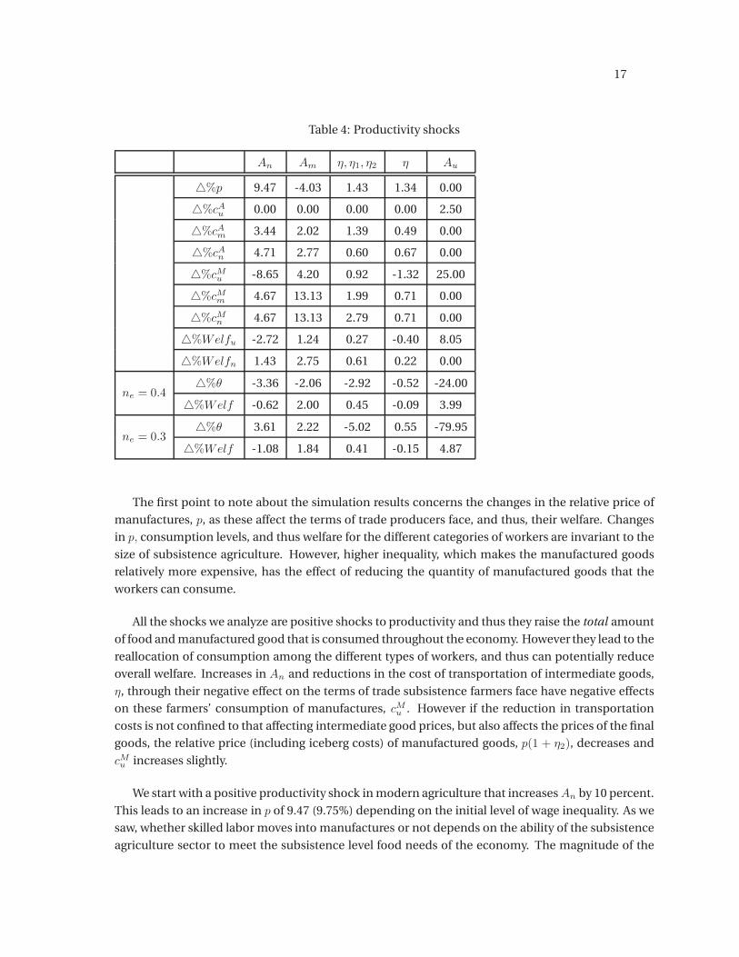
Table 4: Productivity shocks

An Am η, η1, η2 η Au

%p 9.47 -4.03 1.43 1.34 0.00

%cAu 0.00 0.00 0.00 0.00 2.50

%cAm 3.44 2.02 1.39 0.49 0.00

%cAn 4.71 2.77 0.60 0.67 0.00

%cMu -8.65 4.20 0.92 -1.32 25.00

%cMm 4.67 13.13 1.99 0.71 0.00

%cMn 4.67 13.13 2.79 0.71 0.00

%Welfu -2.72 1.24 0.27 -0.40 8.05

%Welfn 1.43 2.75 0.61 0.22 0.00

ne = 0.4%θ -3.36 -2.06 -2.92 -0.52 -24.00

%Welf -0.62 2.00 0.45 -0.09 3.99

ne = 0.3%θ 3.61 2.22 -5.02 0.55 -79.95

%Welf -1.08 1.84 0.41 -0.15 4.87

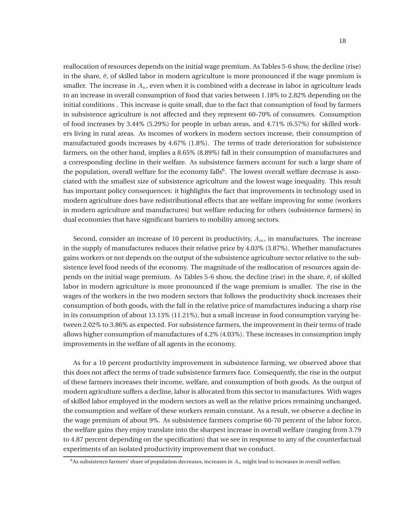
The first point to note about the simulation results concerns the changes in the relative price of

manufactures, p, as these affect the terms of trade producers face, and thus, their welfare. Changes

in p, consumption levels, and thus welfare for the different categories of workers are invariant to the

size of subsistence agriculture. However, higher inequality, which makes the manufactured goods

relatively more expensive, has the effect of reducing the quantity of manufactured goods that the

workers can consume.

All the shocks we analyze are positive shocks to productivity and thus they raise the total amount

of food and manufactured good that is consumed throughout the economy. However they lead to the

reallocation of consumption among the different types of workers, and thus can potentially reduce

overall welfare. Increases in An and reductions in the cost of transportation of intermediate goods,

η, through their negative effect on the terms of trade subsistence farmers face have negative effects

on these farmers’ consumption of manufactures, cMu . However if the reduction in transportation

costs is not confined to that affecting intermediate good prices, but also affects the prices of the final

goods, the relative price (including iceberg costs) of manufactured goods, p(1 + η2), decreases and

cMu increases slightly.

We start with a positive productivity shock in modern agriculture that increasesAn by 10 percent.

This leads to an increase in p of 9.47 (9.75%) depending on the initial level of wage inequality. As we

saw, whether skilled labor moves into manufactures or not depends on the ability of the subsistence

agriculture sector to meet the subsistence level food needs of the economy. The magnitude of the

18

reallocation of resources depends on the initial wage premium. As Tables 5-6 show, the decline (rise)

in the share, θ, of skilled labor in modern agriculture is more pronounced if the wage premium is

smaller. The increase in An, even when it is combined with a decrease in labor in agriculture leads

to an increase in overall consumption of food that varies between 1.18% to 2.82% depending on the

initial conditions . This increase is quite small, due to the fact that consumption of food by farmers

in subsistence agriculture is not affected and they represent 60-70% of consumers. Consumption

of food increases by 3.44% (5.29%) for people in urban areas, and 4.71% (6.57%) for skilled work-

ers living in rural areas. As incomes of workers in modern sectors increase, their consumption of

manufactured goods increases by 4.67% (1.8%). The terms of trade deterioration for subsistence

farmers, on the other hand, implies a 8.65% (8.89%) fall in their consumption of manufactures and

a corresponding decline in their welfare. As subsistence farmers account for such a large share of

the population, overall welfare for the economy falls6. The lowest overall welfare decrease is asso-

ciated with the smallest size of subsistence agriculture and the lowest wage inequality. This result

has important policy consequences: it highlights the fact that improvements in technology used in

modern agriculture does have redistributional effects that are welfare improving for some (workers

in modern agriculture and manufactures) but welfare reducing for others (subsistence farmers) in

dual economies that have significant barriers to mobility among sectors.

Second, consider an increase of 10 percent in productivity, Am, in manufactures. The increase

in the supply of manufactures reduces their relative price by 4.03% (3.87%). Whether manufactures

gains workers or not depends on the output of the subsistence agriculture sector relative to the sub-

sistence level food needs of the economy. The magnitude of the reallocation of resources again de-

pends on the initial wage premium. As Tables 5-6 show, the decline (rise) in the share, θ, of skilled

labor in modern agriculture is more pronounced if the wage premium is smaller. The rise in the

wages of the workers in the two modern sectors that follows the productivity shock increases their

consumption of both goods, with the fall in the relative price of manufactures inducing a sharp rise

in its consumption of about 13.13% (11.21%), but a small increase in food consumption varying be-

tween 2.02% to 3.86% as expected. For subsistence farmers, the improvement in their terms of trade

allows higher consumption of manufactures of 4.2% (4.03%). These increases in consumption imply

improvements in the welfare of all agents in the economy.

As for a 10 percent productivity improvement in subsistence farming, we observed above that

this does not affect the terms of trade subsistence farmers face. Consequently, the rise in the output

of these farmers increases their income, welfare, and consumption of both goods. As the output of

modern agriculture suffers a decline, labor is allocated from this sector to manufactures. With wages

of skilled labor employed in the modern sectors as well as the relative prices remaining unchanged,

the consumption and welfare of these workers remain constant. As a result, we observe a decline in

the wage premium of about 9%. As subsistence farmers comprise 60-70 percent of the labor force,

the welfare gains they enjoy translate into the sharpest increase in overall welfare (ranging from 3.79

to 4.87 percent depending on the specification) that we see in response to any of the counterfactual

experiments of an isolated productivity improvement that we conduct.

6As subsistence farmers’ share of population decreases, increases in An might lead to increases in overall welfare.

19

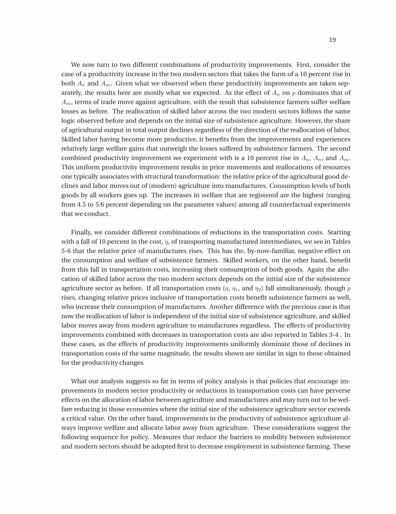
We now turn to two different combinations of productivity improvements. First, consider the

case of a productivity increase in the two modern sectors that takes the form of a 10 percent rise in

both An and Am. Given what we observed when these productivity improvements are taken sep-

arately, the results here are mostly what we expected. As the effect of An on p dominates that of

Am, terms of trade move against agriculture, with the result that subsistence farmers suffer welfare

losses as before. The reallocation of skilled labor across the two modern sectors follows the same

logic observed before and depends on the initial size of subsistence agriculture. However, the share

of agricultural output in total output declines regardless of the direction of the reallocation of labor.

Skilled labor having become more productive, it benefits from the improvements and experiences

relatively large welfare gains that outweigh the losses suffered by subsistence farmers. The second

combined productivity improvement we experiment with is a 10 percent rise in Au, An, and Am.

This uniform productivity improvement results in price movements and reallocations of resources

one typically associates with structural transformation: the relative price of the agricultural good de-

clines and labor moves out of (modern) agriculture into manufactures. Consumption levels of both

goods by all workers goes up. The increases in welfare that are registered are the highest (ranging

from 4.5 to 5.6 percent depending on the parameter values) among all counterfactual experiments

that we conduct.

Finally, we consider different combinations of reductions in the transportation costs. Starting

with a fall of 10 percent in the cost, η, of transporting manufactured intermediates, we see in Tables

5-6 that the relative price of manufactures rises. This has the, by-now-familiar, negative effect on

the consumption and welfare of subsistence farmers. Skilled workers, on the other hand, benefit

from this fall in transportation costs, increasing their consumption of both goods. Again the allo-

cation of skilled labor across the two modern sectors depends on the initial size of the subsistence

agriculture sector as before. If all transportation costs (η, η1, and η2) fall simultaneously, though p

rises, changing relative prices inclusive of transportation costs benefit subsistence farmers as well,

who increase their consumption of manufactures. Another difference with the previous case is that

now the reallocation of labor is independent of the initial size of subsistence agriculture, and skilled

labor moves away from modern agriculture to manufactures regardless. The effects of productivity

improvements combined with decreases in transportation costs are also reported in Tables 3-4 . In

these cases, as the effects of productivity improvements uniformly dominate those of declines in

transportation costs of the same magnitude, the results shown are similar in sign to those obtained

for the productivity changes.

What our analysis suggests so far in terms of policy analysis is that policies that encourage im-

provements in modern sector productivity or reductions in transportation costs can have perverse

effects on the allocation of labor between agriculture and manufactures and may turn out to be wel-

fare reducing in those economies where the initial size of the subsistence agriculture sector exceeds

a critical value. On the other hand, improvements in the productivity of subsistence agriculture al-

ways improve welfare and allocate labor away from agriculture. These considerations suggest the

following sequence for policy. Measures that reduce the barriers to mobility between subsistence

and modern sectors should be adopted first to decrease employment in subsistence farming. These

20

can be implemented simultaneously with policies that encourage adoption of improved technolo-

gies in subsistence farming. It is only after the share of employment in the subsistence sector has

declined that policies that incentivize agents to adopt more productive technologies in the modern

sectors or that lower transportation costs should be implemented.

4. Conclusion

Many poor developing countries have relatively large parts of their labor force employed in agri-

culture. Though some of these workers are employed by farms using modern agricultural equip-

ment and technology, a significantly high share of agricultural employment remains in subsistence

or quasi-subsistence agriculture, using traditional technologies with low productivity. Why these

countries have such large fractions of their workers in agriculture remains an open question.

Our paper suggests that a number of mechanisms may help answer this question. First, barriers

to labor mobility from the subsistence farming hinterland to the modern sectors (taking perhaps a

number of forms including high costs of skill acquisition, as well as cultural and institutional restric-

tions) would help explain why employment in the subsistence sector remains high. Second, produc-

tivity differences and transportation costs play an important role but not necessarily in the direc-

tion suggested by the existing literature. We show, among others, that productivity improvements

in modern agriculture may actually increase the employment share of agriculture in those countries

where subsistence agriculture is initially large. Similarly reductions in certain transportation costs

may increase the employment share of agriculture in these economies. Intuitively, these results that

run counter to the findings in the previous literature arise from the barriers to the movement of la-

bor out of subsistence agriculture as well as the terms of trade effects of changes in productivity and

transportation costs. Such terms of trade effects also have rather significant negative consequences

for subsistence farmers. Further, where such farmers comprise a sizable enough majority of the

population, the welfare losses they suffer outweigh the gains that accrue to the rest of the popula-

tion such that winners cannot compensate the losers. These results suggest that in economies with

significant distortions, second-best welfare paradoxes may be important and policy recommenda-

tions concerning public investment in infrastructure designed to improve productivity in the mod-

ern sectors or lower transportation costs need to be reconsidered. Our model instead would provide

basis for policies designed to improve productivity in subsistence agriculture and lower the cost of

education of subsistence farmers should come first. Once the barriers to labor mobility have been

reduced and the subsistence sector becomes smaller, policies directed at the modern sectors and

transportation costs would have the desired effects.

21

References

Adam, Christopher, David Bevan and Douglas Gollin (2013), “Rural-Urban Linkages, Transaction

Costs, and Poverty Alleviation: The Case of Tanzania”, Unpublished manuscript, Oxford University.

Adamopoulos, Tasso (2011), “Transportation costs, agricultural productivity and cross- country

income differences”, International Economic Review, 52 (2): 489–521.

Caselli, Francesco and Wilbur John Coleman II (2001), “The U.S. Structural Transformation and

Regional Convergence: A Reinterpretation”, Journal of Political Economy 109: 584–616.

Chenery, Hollis and Moises Syrguin (1975), “Pattern of Development, 1950-1970”, Oxford Univer-

sity Press for the World Bank.

Clark, Colin (1940) “The Conditions of Economic Progress”, Macmillan and Co, London.

Eberhardt, Markus and Francis Teal (2013), “Structural change and cross-country growth empir-

ics”, World Bank Policy Research Working Paper 6335.

Foster, Andrew and Mark Rosenzweig (1996), “Technical Change and Human-Capital Returns

and Investments: Evidence from the Green Revolution”, American Economic Review 86(4): 931-53.

Gollin, Douglas, Stephen Parente and Richard Rogerson (2004) “Farm work, home work and in-

ternational productivity differences”, Review of Economic Dynamics 7: 827-850.

Gollin, Douglas, David Lagakos and Michael E. Waugh (2014) “The Agricultural Productivity Gap”,

The Quarterly Journal of Economics, 129 (2): 939-993.

Gollin, Douglas and Richard Rogerson, (2014) " Productivity, transport costs and subsistence agri-

culture”, Journal of Development Economics, 107: 38-48.

Herrendorf, Berthold, Schmitz, James A., Teixeira, Arilton, (2012), “The role of transportation in

U.S. economic development: 1840–1860”, International Economic Review 53 (3): 693–715.

Kuznets, Simon (1966), Modern economic growth, New Haven, CT: Yale University Press.

Larson, Donald and Yair Mundlak (1997), “On the intersectoral migration of agricultural labor”,

Economic Development and Cultural Change 45 (2): 295-319.

McMilan, Margaret and Dani Rodrik, (2011), “Globalization, Structural Change and Productivity

Growth”, NBER Working Papers 17143.

22

Mundlak, Yair, Rita Butzer and Donald Larson (2012), “Heterogeneous technology and panel

data: The case of the agricultural production function”, Journal of Development Economics, 99(1):

139-149.

O’Brien, P.K. (1996), “Path Dependency, or Why Britain Became an Industrialized and Urbanized

Economy Long before France”, The Economic History Review, 49(2): 213-249.

Parente, Stephen L. and Edward C. Prescott (2005), “A Unified Theory of the Evolution of Interna-

tional Income Levels” in Handbook of Economic Growth 1(B): 1373-1416.

Restuccia, Diego, Dennis Tao Yang, and Xiaodong Zhu (2008) “Agriculture and Aggregate Produc-

tivity: A Quantitative Cross-Country Analysis.” Journal of Monetary Economics, 55(2): 234–50.

Young, Alwyn (2013), ‘‘Inequality, the Urban-Rural Gap and Migration,’’ Quarterly Journal of Eco-

nomics , 128 (2013): 1727–1785.

23

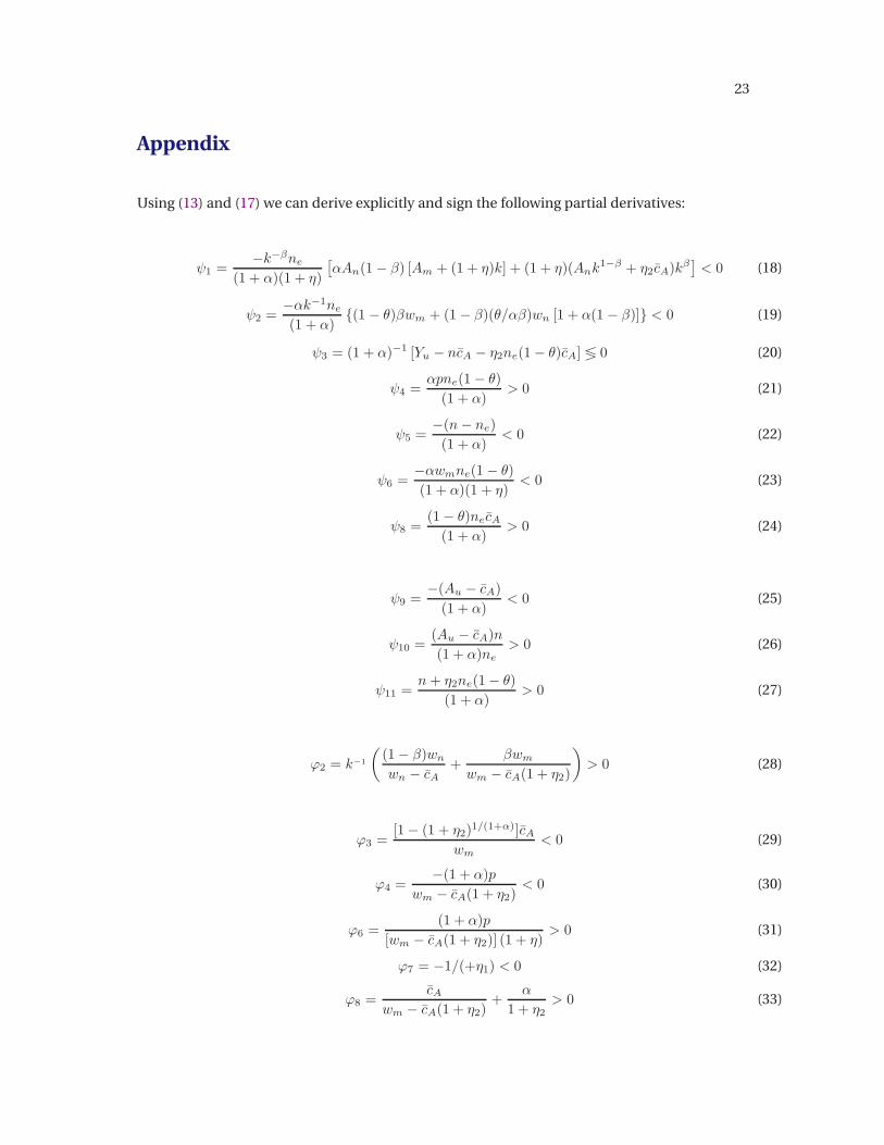
Appendix

Using (13) and (17) we can derive explicitly and sign the following partial derivatives:

ψ1 =−k−βne

(1 + α)(1 + η)

[

αAn(1− β) [Am + (1 + η)k] + (1 + η)(Ank1−β + η2cA)k

β]

< 0 (18)

ψ2 =−αk−1ne

(1 + α)(1 − θ)βwm + (1− β)(θ/αβ)wn [1 + α(1 − β)] < 0 (19)

ψ3 = (1 + α)−1 [Yu − ncA − η2ne(1− θ)cA] ≶ 0 (20)

ψ4 =αpne(1− θ)

(1 + α)> 0 (21)

ψ5 =−(n− ne)

(1 + α)< 0 (22)

ψ6 =−αwmne(1 − θ)

(1 + α)(1 + η)< 0 (23)

ψ8 =(1− θ)necA(1 + α)

> 0 (24)

ψ9 =−(Au − cA)

(1 + α)< 0 (25)

ψ10 =(Au − cA)n

(1 + α)ne> 0 (26)

ψ11 =n+ η2ne(1− θ)

(1 + α)> 0 (27)

ϕ2 = k−1

(

(1− β)wn

wn − cA+

βwm

wm − cA(1 + η2)

)

> 0 (28)

ϕ3 =[1− (1 + η2)

1/(1+α)]cAwm

< 0 (29)

ϕ4 =−(1 + α)p

wm − cA(1 + η2)< 0 (30)

ϕ6 =(1 + α)p

[wm − cA(1 + η2)] (1 + η)> 0 (31)

ϕ7 = −1/(+η1) < 0 (32)

ϕ8 =cA

wm − cA(1 + η2)+

α

1 + η2> 0 (33)

24

ϕ11 =(1 + α)

wm − cA(1 + η2)

[

(1 + η2)−wm − cA(1 + η2)

wn − ca

]

> 0 if η1 = η2 (34)

Analytics of Comparative Statics

General results for the effects of changes in parameters on k andθ are given by

dk

dxj= −

ϕjψ1

∆,dθ

dxj=

−ϕ2ψj + ϕjψ2

∆, ∆ := ϕ2ψ1 < 0 (35)

for parameter xj (j ∈ 3, .., 11) in equations (18) to (34).

Analytically clean results can be obtained by setting initial values of transportation costs η1 and

η2 equal to zero. In this case using (12)-(17) we derive

Yu − ncA = Yn

(

αβ − θ

θ− 1

)

(36)

which is ≥ (<)0 depending on the size of subsistence agriculture Yu ≥ (<)ncA.

We can then obtain:

wn = wm (37)

Yn =

(

1− β

β

)1−β (Am

1 + η

)1−β

Anθne (38)

z = θneAm1− β

β(1 + η)(39)

p =

(

1− β

1 + η

)1−β (βnAm

)β

An (40)

Thus, we can derive the comparative static results concerning the effects of changes in Am, An,

Au, η, and ne on the variables of interest θ, z, and p.

Proof of Lemma 1:

∂θ

∂Am=

1− β

1 + α

θ

Am

(

αβ − θ

θ− 1

)

≥ (<)0 (41)

if Yu ≥ (<)ncA.

25

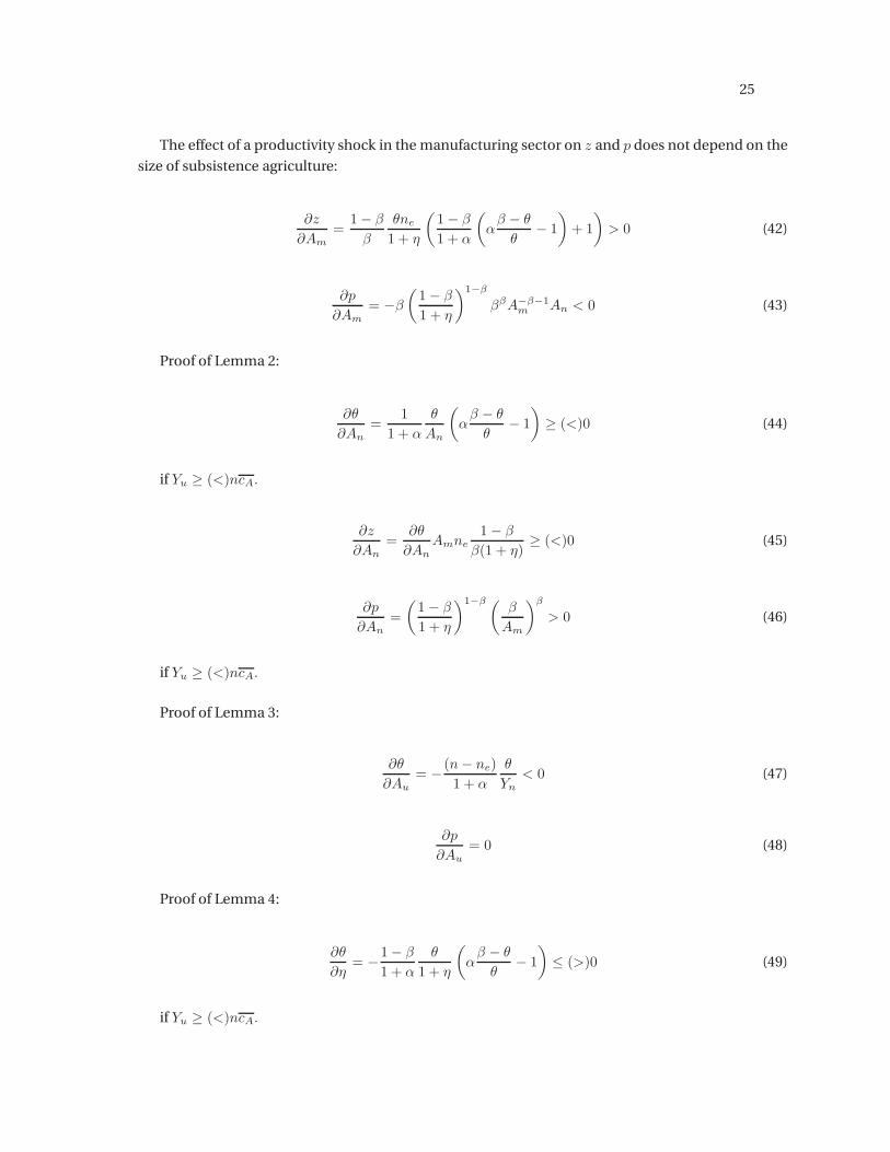
The effect of a productivity shock in the manufacturing sector on z and p does not depend on the

size of subsistence agriculture:

∂z

∂Am=

1− β

β

θne

1 + η

(

1− β

1 + α

(

αβ − θ

θ− 1

)

+ 1

)

> 0 (42)

∂p

∂Am= −β

(

1− β

1 + η

)1−β

ββA−β−1m An < 0 (43)

Proof of Lemma 2:

∂θ

∂An=

1

1 + α

θ

An

(

αβ − θ

θ− 1

)

≥ (<)0 (44)

if Yu ≥ (<)ncA.

∂z

∂An=

∂θ

∂AnAmne

1− β

β(1 + η)≥ (<)0 (45)

∂p

∂An=

(

1− β

1 + η

)1−β (β

Am

)β

> 0 (46)

if Yu ≥ (<)ncA.

Proof of Lemma 3:

∂θ

∂Au= −

(n− ne)

1 + α

θ

Yn< 0 (47)

∂p

∂Au= 0 (48)

Proof of Lemma 4:

∂θ

∂η= −

1− β

1 + α

θ

1 + η

(

αβ − θ

θ− 1

)

≤ (>)0 (49)

if Yu ≥ (<)ncA.

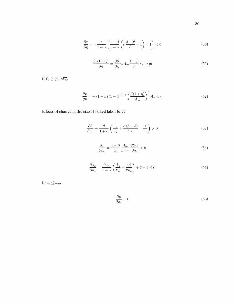
26

∂z

∂η= −

z

1 + η

(

1− β

1 + α

(

αβ − θ

θ− 1

)

+ 1

)

< 0 (50)

∂z(1 + η)

∂η=∂θ

∂ηneAm

1− β

β≤ (>)0 (51)

if Yu ≥ (<)ncA.

∂p

∂η= − (1− β) (1− β)

1−β

(

β(1 + η)

Am

)β

An < 0 (52)

Effects of change in the size of skilled labor force:

∂θ

∂ne=

θ

1 + α

(

Au

Yn+α(β − θ)

θne−

1

ne

)

> 0 (53)

∂z

∂ne=

1− β

β

Am

1 + η

∂θne

∂ne> 0 (54)

∂na

∂ne=

θne

1 + α

(

Au

Yn+αβ

θne

)

+ θ − 1 ≤ 0 (55)

if wu ≤ wn.

∂p

∂ne= 0 (56)

27

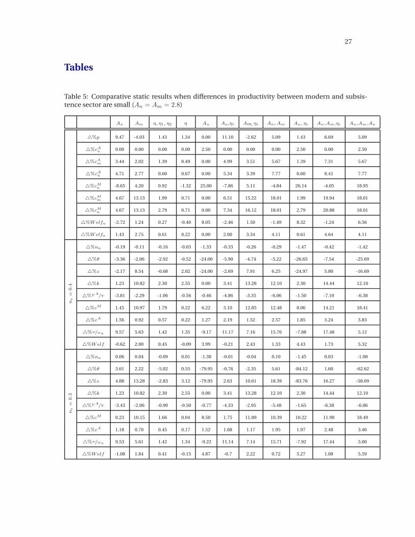
Tables

Table 5: Comparative static results when differences in productivity between modern and subsis-tence sector are small (An = Am = 2.8)

An Am η, η1, η2 η Au An,ηi Am,ηi An, Am Au, ηi An,Am,ηi An,Am,Au

%p 9.47 -4.03 1.43 1.34 0.00 11.10 -2.62 5.09 1.43 6.69 5.09

%cAu 0.00 0.00 0.00 0.00 2.50 0.00 0.00 0.00 2.50 0.00 2.50

%cAm 3.44 2.02 1.39 0.49 0.00 4.99 3.51 5.67 1.39 7.31 5.67

%cAn 4.71 2.77 0.60 0.67 0.00 5.34 3.39 7.77 0.60 8.41 7.77

%cMu -8.65 4.20 0.92 -1.32 25.00 -7.86 5.11 -4.84 26.14 -4.05 18.95

%cMm 4.67 13.13 1.99 0.71 0.00 6.51 15.22 18.01 1.99 19.94 18.01

%cMn 4.67 13.13 2.79 0.71 0.00 7.34 16.12 18.01 2.79 20.88 18.01

%Welfu -2.72 1.24 0.27 -0.40 8.05 -2.46 1.50 -1.49 8.32 -1.24 6.56

%Welfn 1.43 2.75 0.61 0.22 0.00 2.00 3.34 4.11 0.61 4.64 4.11

ne=

0.4

%na -0.19 -0.11 -0.16 -0.03 -1.33 -0.33 -0.26 -0.29 -1.47 -0.42 -1.42

%θ -3.36 -2.06 -2.92 -0.52 -24.00 -5.90 -4.74 -5.22 -26.65 -7.54 -25.69

%z -2.17 8.54 -0.68 2.02 -24.00 -2.69 7.91 6.25 -24.97 5.80 -16.69

%k 1.23 10.82 2.30 2.55 0.00 3.41 13.28 12.10 2.30 14.44 12.10

%Y A/Y -3.81 -2.29 -1.06 -0.56 -0.46 -4.86 -3.35 -6.06 -1.50 -7.10 -6.38

%cM 1.45 10.97 1.79 0.22 6.22 3.10 12.85 12.48 8.06 14.21 18.41

%cA 1.56 0.92 0.57 0.22 1.27 2.19 1.52 2.57 1.85 3.24 3.83

%w/wu 9.57 5.63 1.42 1.35 -9.17 11.17 7.16 15.76 -7.88 17.48 5.12

%Welf -0.62 2.00 0.45 -0.09 3.99 -0.21 2.43 1.33 4.43 1.73 5.32

ne=

0.3

%na 0.06 0.04 -0.09 0.01 -1.38 -0.01 -0.04 0.10 -1.45 0.03 -1.08

%θ 3.61 2.22 -5.02 0.55 -79.95 -0.76 -2.35 5.61 -84.12 1.60 -62.62

%z 4.88 13.28 -2.83 3.12 -79.95 2.63 10.61 18.39 -83.76 16.27 -58.09

%k 1.23 10.82 2.30 2.55 0.00 3.41 13.28 12.10 2.30 14.44 12.10

%Y A/Y -3.43 -2.06 -0.90 -0.50 -0.77 -4.33 -2.95 -5.48 -1.65 -6.38 -6.06

%cM 0.23 10.15 1.66 0.04 8.50 1.75 11.89 10.39 10.22 11.98 18.49

%cA 1.18 0.70 0.45 0.17 1.52 1.68 1.17 1.95 1.97 2.48 3.46

%w/wu 9.53 5.61 1.42 1.34 -9.22 11.14 7.14 15.71 -7.92 17.44 5.00

%Welf -1.08 1.84 0.41 -0.15 4.87 -0.7 2.22 0.72 5.27 1.08 5.59

28

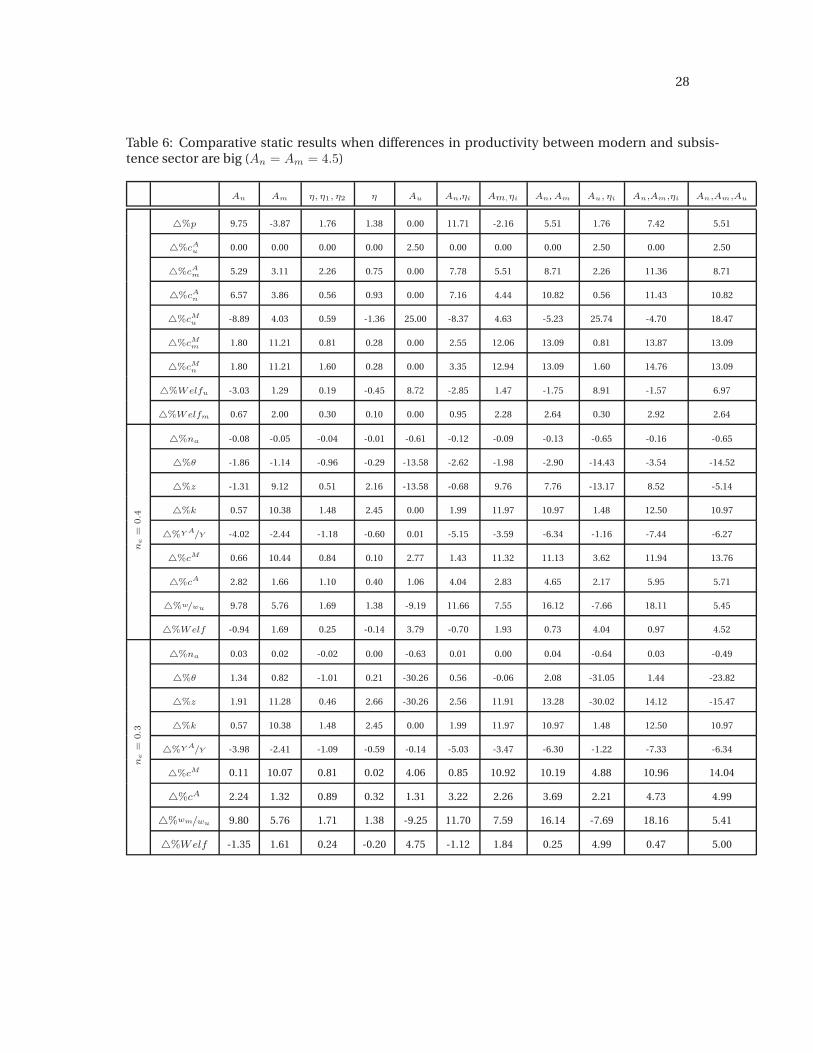
Table 6: Comparative static results when differences in productivity between modern and subsis-tence sector are big (An = Am = 4.5)

An Am η, η1, η2 η Au An,ηi Am,ηi An, Am Au, ηi An,Am,ηi An,Am,Au

%p 9.75 -3.87 1.76 1.38 0.00 11.71 -2.16 5.51 1.76 7.42 5.51

%cAu 0.00 0.00 0.00 0.00 2.50 0.00 0.00 0.00 2.50 0.00 2.50

%cAm 5.29 3.11 2.26 0.75 0.00 7.78 5.51 8.71 2.26 11.36 8.71

%cAn 6.57 3.86 0.56 0.93 0.00 7.16 4.44 10.82 0.56 11.43 10.82

%cMu -8.89 4.03 0.59 -1.36 25.00 -8.37 4.63 -5.23 25.74 -4.70 18.47

%cMm 1.80 11.21 0.81 0.28 0.00 2.55 12.06 13.09 0.81 13.87 13.09

%cMn 1.80 11.21 1.60 0.28 0.00 3.35 12.94 13.09 1.60 14.76 13.09

%Welfu -3.03 1.29 0.19 -0.45 8.72 -2.85 1.47 -1.75 8.91 -1.57 6.97

%Welfm 0.67 2.00 0.30 0.10 0.00 0.95 2.28 2.64 0.30 2.92 2.64

ne=

0.4

%na -0.08 -0.05 -0.04 -0.01 -0.61 -0.12 -0.09 -0.13 -0.65 -0.16 -0.65

%θ -1.86 -1.14 -0.96 -0.29 -13.58 -2.62 -1.98 -2.90 -14.43 -3.54 -14.52

%z -1.31 9.12 0.51 2.16 -13.58 -0.68 9.76 7.76 -13.17 8.52 -5.14

%k 0.57 10.38 1.48 2.45 0.00 1.99 11.97 10.97 1.48 12.50 10.97

%Y A/Y -4.02 -2.44 -1.18 -0.60 0.01 -5.15 -3.59 -6.34 -1.16 -7.44 -6.27

%cM 0.66 10.44 0.84 0.10 2.77 1.43 11.32 11.13 3.62 11.94 13.76

%cA 2.82 1.66 1.10 0.40 1.06 4.04 2.83 4.65 2.17 5.95 5.71

%w/wu 9.78 5.76 1.69 1.38 -9.19 11.66 7.55 16.12 -7.66 18.11 5.45

%Welf -0.94 1.69 0.25 -0.14 3.79 -0.70 1.93 0.73 4.04 0.97 4.52

ne=

0.3

%na 0.03 0.02 -0.02 0.00 -0.63 0.01 0.00 0.04 -0.64 0.03 -0.49

%θ 1.34 0.82 -1.01 0.21 -30.26 0.56 -0.06 2.08 -31.05 1.44 -23.82

%z 1.91 11.28 0.46 2.66 -30.26 2.56 11.91 13.28 -30.02 14.12 -15.47

%k 0.57 10.38 1.48 2.45 0.00 1.99 11.97 10.97 1.48 12.50 10.97

%Y A/Y -3.98 -2.41 -1.09 -0.59 -0.14 -5.03 -3.47 -6.30 -1.22 -7.33 -6.34

%cM 0.11 10.07 0.81 0.02 4.06 0.85 10.92 10.19 4.88 10.96 14.04

%cA 2.24 1.32 0.89 0.32 1.31 3.22 2.26 3.69 2.21 4.73 4.99

%wm/wu 9.80 5.76 1.71 1.38 -9.25 11.70 7.59 16.14 -7.69 18.16 5.41

%Welf -1.35 1.61 0.24 -0.20 4.75 -1.12 1.84 0.25 4.99 0.47 5.00

! 29!

!!

!!

Figure!1:!Increase!in!the!number!of!skilled!workers!ne!!

!!

Figure!2:!Increase!in!manufacturing!productivity!Am!!

!!

k

Unm = 0

zz

EDA = 0

pθθL θH

Unm = 0

zz

EDA = 0

k

p θp0 p1

k0

k1

θ′LθL θHθ′

H

Figures

! 30!

!!!

!!

Figure!3:!Increase!in!the!productivity!of!the!modern!agriculture!sector!An!!

!

!!

Figure!4:!Decrease!in!the!cost!of!transportation! !

k

Unm = 0

zz

EDA = 0

p

θ

p0p1

k0

k1

θL θ′L

θHθ′H

Unm = 0

zz

EDA = 0

k

p θp0p1

k0

k1

θ′LθL θHθ′

H