Embed Size (px)
Citation preview

No.10-E-11 October 2010
The Role of Money and Growth Expectations in Price Determination Mechanism Takeshi Kimura* [email protected]
Takeshi Shimatani* [email protected]
Kenichi Sakura† [email protected]
Tomoaki Nishida* [email protected]
Bank of Japan 2-1-1 Nihonbashi-Hongokucho, Chuo-ku, Tokyo 103-0021, Japan
* International Department † Research and Statistics Department
Papers in the Bank of Japan Working Paper Series are circulated in order to stimulate discussion and comments. Views expressed are those of authors and do not necessarily reflect those of the Bank. If you have any comment or question on the working paper series, please contact each author. When making a copy or reproduction of the content for commercial purposes, please contact the Public Relations Department ([email protected]) at the Bank in advance to request permission. When making a copy or reproduction, the source, Bank of Japan Working Paper Series, should explicitly credited.
Bank of Japan Working Paper Series
The Role of Money and Growth Expectations in Price Determination Mechanism ∗
Takeshi Kimura*, Takeshi Shimatani**, Kenichi Sakura†, Tomoaki Nishida***
October 2010
Abstract There is a positive cross-country correlation between money growth and inflation rate, and both money growth and inflation rate of Japan are lower than those of other advanced countries. In the “Money view” based on the quantity theory of money, it can be interpreted that Japan’s low inflation results from the low growth of money. However, the time-series correlation between money growth and inflation rate in advanced countries including Japan has declined since the mid 1990s. Furthermore, during this period, a strong positive correlation between the potential growth rate and the long-term inflation expectation is observed in Japan, and these facts are not consistent with the Money view. Japan’s potential growth rate declined sharply in the past two decades in contrast to other advanced countries, and as a result expectations for future economic growth also declined, which may possibly have caused deflation in Japan. In the “Expected Burden view” based on the fiscal theory of the price level, growth expectations affect the price level as follows: 1) the decline in growth expectations increases the future fiscal burden on the private sector; 2) the private sector then cuts its expenditures to increase savings for the future burdens; 3) as a result, the aggregate demand decreases and hence the aggregate price level falls. This paper examines whether such a mechanism has indeed worked in Japan or not, comparing the inflation developments in the US and the euro area.
Keywords: Money view, Expected Burden view
We are grateful for helpful discussions and comments from Kosuke Aoki, Hidetaka Enomoto, Kunio Okina, Masashi Saito, Toshitaka Sekine, Shinobu Nakagawa, Yoshinori Nakata, Yasuhiro Hayasaki, Hiroshi Fujiki, Ippei Fujiwara, Ichiro Muto, and Shingo Watanabe. We also thank Ryota Nakatani, Hiroyuki Egami, and Yuki Masujima for their excellent research assistance. Any remaining errors are the sole responsibility of the authors. The views expressed herein are those of the authors and should not be interpreted as those of the Bank of Japan. * International Department, Bank of Japan; E-mail: [email protected] ** International Department, Bank of Japan; E-mail: [email protected] † Research and Statistics Department, Bank of Japan; E-mail: [email protected] *** International Department, Bank of Japan; E-mail: [email protected]

1
1. Introduction In the US and the euro area, where the core CPI inflation rates have declined recently,
there are growing concerns about whether disinflation will continue going forward and
proceed to a deflationary situation, or whether disinflation will be restrained and the
inflation rates will reverse the downward trend. Phillips curve may help us to answer
this kind of question because we can forecast inflation rates by substituting the projected
output gap into the Phillips curve. Japan’s inflation rate can be also forecasted by the
same method.
Although Phillips curve is a useful model to forecast inflation rates, it is important
to examine price fluctuations through several perspectives rather than the single
approach of the Phillips curve. In addition, while the Phillips curve is effective in
explaining price fluctuations over the short term, it may not necessarily be appropriate
for explaining price fluctuations over the long term. That is, when we forecast inflation
rates over the coming 1-2 years by using Phillips curve, we need to assume that the
long-term expected inflation rate is exogenously given. The Phillips curve alone cannot
lead to an answer about how the inflation rate (and expected inflation) will change over
the long term.
The purpose of this paper is to examine price fluctuations from a long-term
perspective rather than from a short-term perspective. Because prices are flexible in the
long-run, the actual inflation rate is equal to the expected inflation rate, and the output
gap is zero. Therefore, the Phillips curve, into which the expected inflation and the
output gap are substituted, is ineffective to explain the long-run price fluctuations. This
paper examines the two views about the long-run price determination mechanism: 1) the
“Money view,” where changes in money affect the price level; and 2) the “Expected
Burden view,” where changes in growth expectations affect the price level via changes
in the fiscal burdens and the debt burdens of the private sector.
The remainder of the paper proceeds as follows. Section 2 presents several facts
about price fluctuations in advanced countries, and Section 3 raises issues to be
discussed. Section 4 explains the two views about the long-run price determination
mechanism. Section 5 and 6 examine price fluctuations in the US, the euro area, and
Japan. Finally, Section 7 concludes.

2
2. Fact-findings: Relationship among the Inflation Rate, Money Growth, and Real Growth Rate
In this section, we present four facts about price fluctuations in advanced countries,
focusing on the relationship among the inflation rate, money growth, and real output
growth rate. Note that “money” in this paper refers to broadly defined money stock such
as M2 and M3, and not the monetary base.
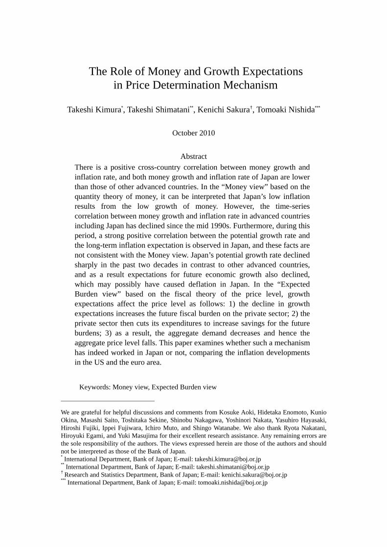
Fact 1. Adjusted money growth rates(*) and inflation rates averaged on a ten-year
basis in the OECD countries show a positive cross-country correlation in all sample
periods (Figure 1). That is, in the countries with higher inflation, money growth is
higher and in contrast, in the countries with lower inflation, money growth is lower.
Note that both money growth and inflation rate of Japan are lower than those of other
advanced countries. (*) Adjusted money growth is defined as money growth minus real GDP growth.
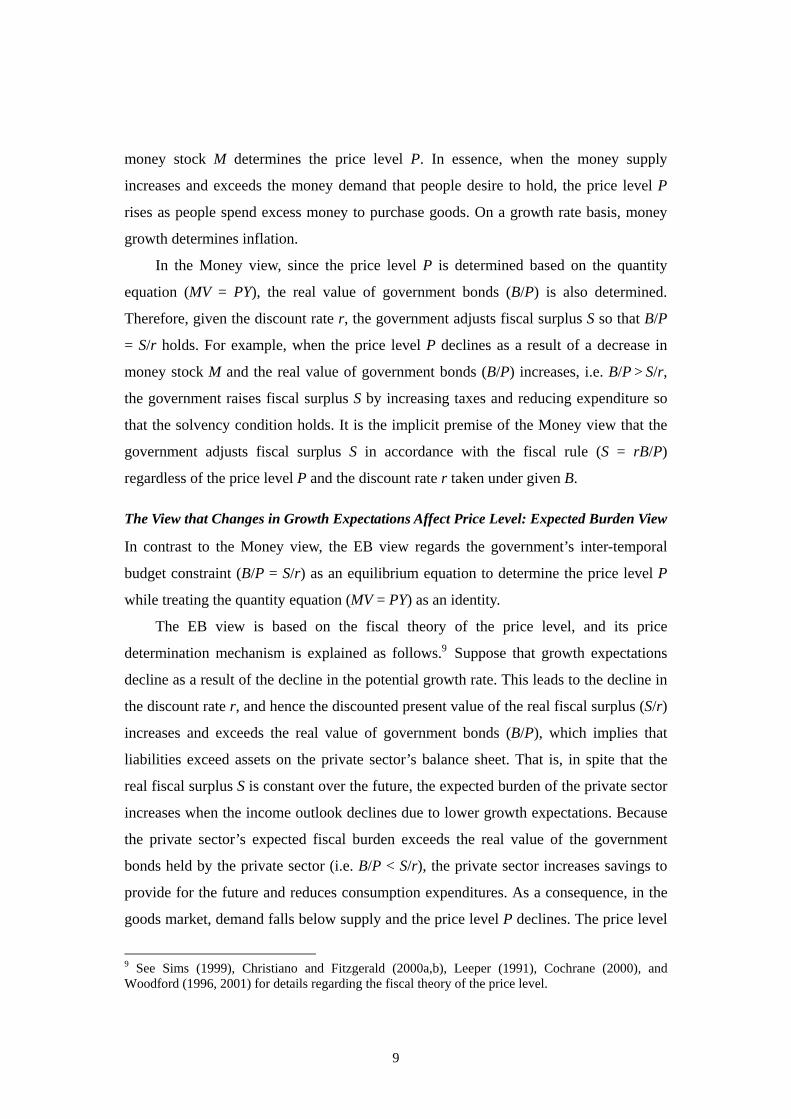
Fact 2. The time-series relationship between adjusted money growth and inflation rate
in advanced countries shows a positive correlation from the 1970s to the first half of the
1990s (Figure 2). However, the time-series correlation between them declined after the
Figure 1. Cross-country Correlation between Money Growth and Inflation
1970’s 1980’s 1990’s 2000’s
Notes. 1. Money growth and inflation rate are changes in M3 and GDP deflator, respectively. Data for 2000’s are up to 2008 except for
the US whose money growth is only available up to 2005. 2. The sample countries are OECD countries. The number of sample countries differs across decades because of data availability. Sources. International Monetary Fund, “International Financial Statistics”, OECD, Each country’s statistics.
-5
0
5
10
15
20
25
30
-5 0 5 10 15 20 25 30
France(FR)
Germany(DE)US
Correlation 0.90
Infla
tion
Rate
(%)
Adjusted Money Growth (%)
-5
0
5
10
15
20
25
30
-5 0 5 10 15 20 25 30
JP
FR
DEUS UK
Correlation 0.78
-5
0
5
10
15
20
25
30
-5 0 5 10 15 20 25 30
Correlation 0.92
UK
DEUS
FR JP-5
0
5
10
15
20
25
30
-5 0 5 10 15 20 25 30
Correlation 0.92
DE
FRUS
JPUK
Japan(JP)

3
latter half of the 1990s in all advanced countries.1 This is because inflation rates remain
relatively stable even when the money growth fluctuates more significantly than the real
output growth.
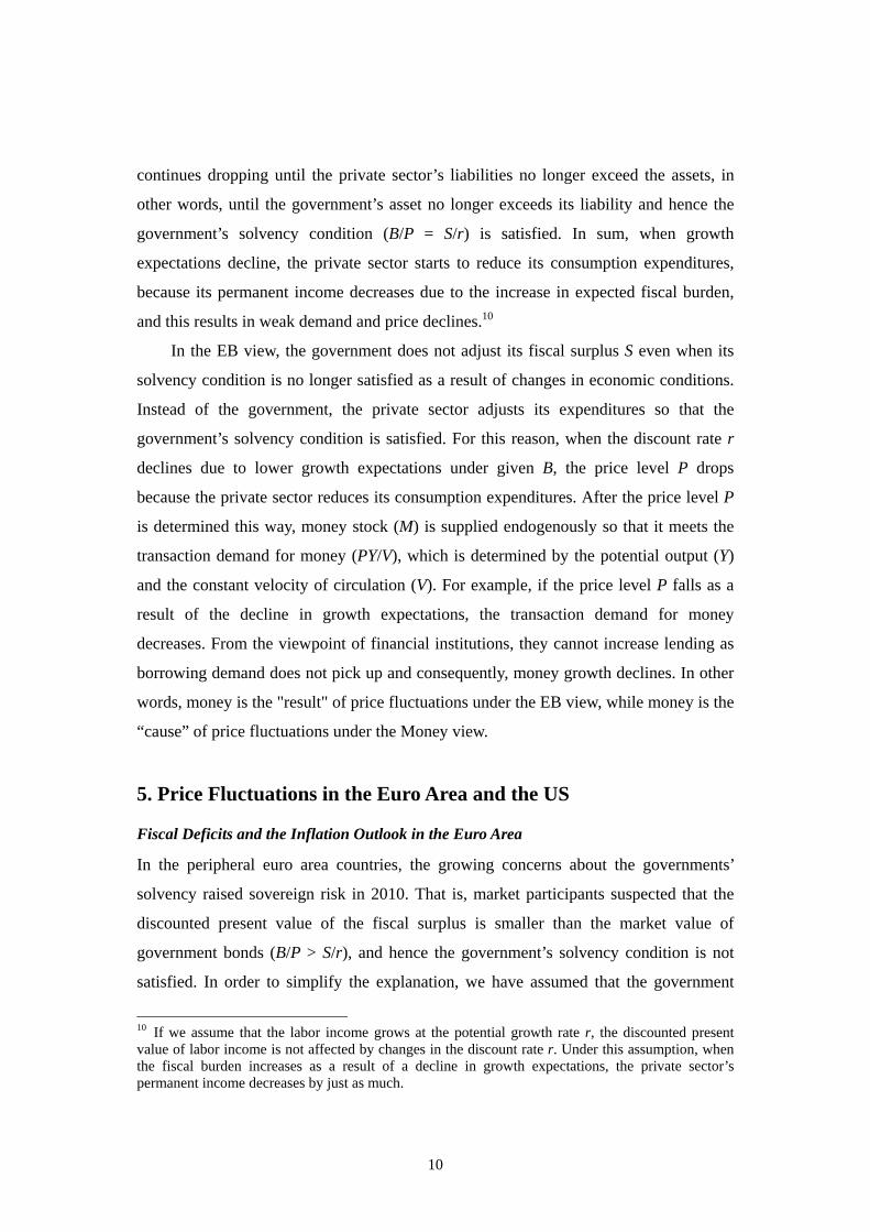
Fact 3. Next, we focus on the relationship between the real output growth and
inflation, not the relationship between money growth and inflation. Real GDP growth
1 See Bank of Japan (2003) for how the time-series correlation between money growth and the inflation rate decreased in Japan since the mid 1990s.
Figure 2. Money Growth and Inflation in Advanced Countries
United States France United Kingdom Japan
Notes. 1. Figures in parentheses are correlation coefficients of 1970-1994 and 1995-2009. Money growth is based on M2 for the US and
Japan, M3 for France, and M4 for the UK, respectively. Each money indicator is chosen because of the availability of long time-series data.
2. Because of the data discontinuity of Germany in 1990’s, France is selected as the representative of the euro area. Sources. International Monetary Fund, “International Financial Statistics”, Eurostat, Each country’s statistics.
-5
0
5
10
15
70 80 90 00Adjusted Money Growth (%) Inflation Rate (%)
(-0.31)(0.62)
%
-5
0
5
10
15
20
25
30
70 80 90 00
(-0.08)(0.49)
-5
0
5
10
15
20
25
70 80 90 00
(0.21)(0.67)
%
-5
0
5
10
15
20
25
70 80 90 00
(0.42)(0.76)
% %
Figure 3. Inflation and Real Output Growth Rate
1970’s 1980’s 1990’s 2000’s
Notes. 1. Inflation rate is measured by GDP Deflator. 2. The sample countries are OECD countries. The number of sample countries differs across decades because of data availability.Source. International Monetary Fund, “International Financial Statistics”.
-5
0
5
10
15
20
25
-2 0 2 4 6 8 10
JPFR
DE
UK
US
Correlation 0.51
Infla
tion
Rate
(%)
Real GDP Growth (%)
-5
0
5
10
15
20
25
-2 0 2 4 6 8 10
Correlation -0.25JP
FR
DE
UK
US
-5
0
5
10
15
20
25
-2 0 2 4 6 8 10
DE
JP FR
UK
US
Correlation -0.20
-5
0
5
10
15
20
25
-2 0 2 4 6 8 10
JP
FR
DEUS
UK
Correlation 0.40

4
rates and inflation rates averaged on a 10-year basis in the OECD countries show no or
only a low cross-country correlation in all sample periods (Figure 3). In the long run, the
real GDP growth rate converges to the potential growth rate, and the inflation rate
averaged over the long term is not much affected by the real economy in the advanced
countries as a whole.
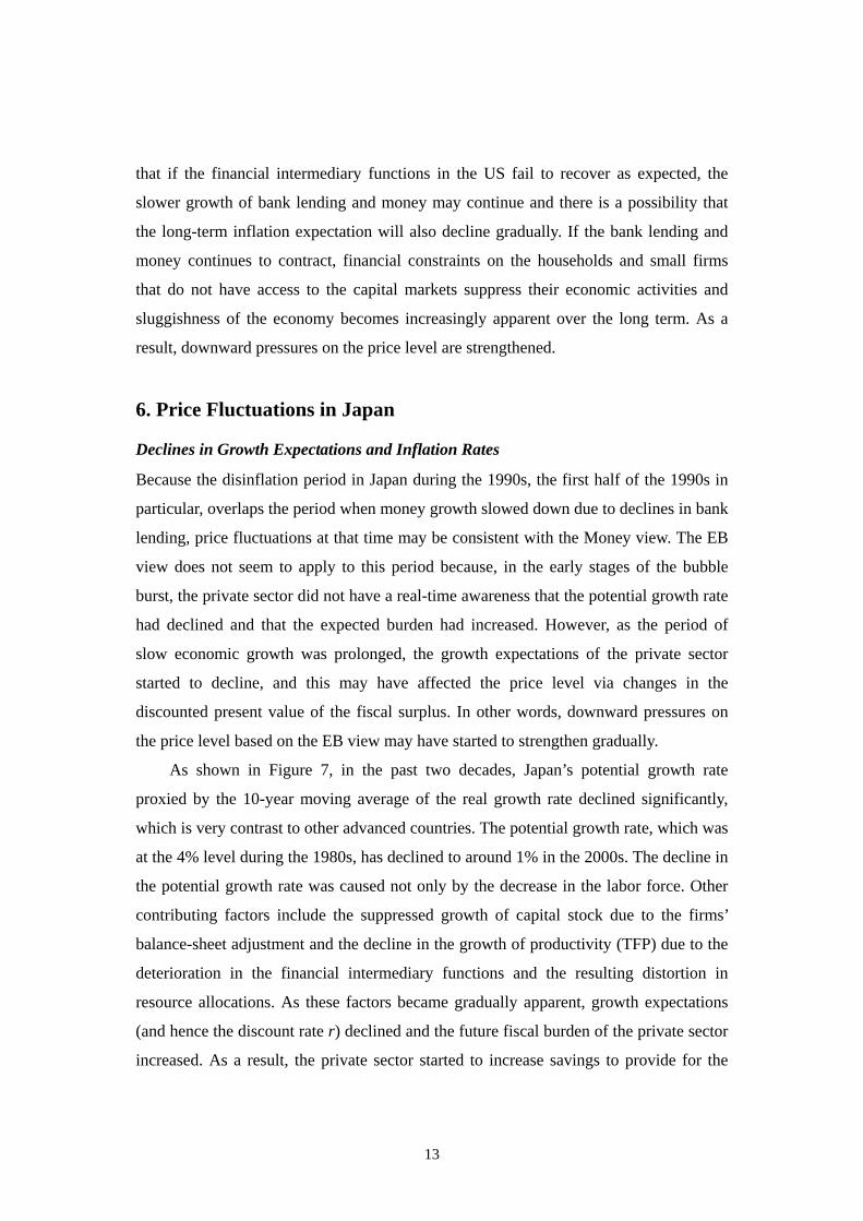
Fact 4. Finally, we examine the relationship between the long-term inflation
expectation and the potential growth rate (Figure 4). The private sector’s inflation
outlook over the coming 5-10 years by the Consensus Forecast is used as the long-term
inflation expectation. In the US, the euro area, and the UK, there is no time-series
correlation between the long-term inflation expectation and the potential growth rate,
which is consistent with Fact 3. However, only in Japan, a strong positive correlation
between them is observed.
3. Issues to be Raised Based on the facts presented above, we raise the following two issues.
Figure 4. Potential Growth Rate and Long-Term Inflation Expectations
Japan United States Euro area United Kingdom
Notes. 1. Long-term inflation expectation for each year is 5-10 years ahead outlook averaged on April and October survey results of
Consensus Forecast. Potential growth rates are measured by BOJ for Japan, CBO for the US, and the Hodrick-Prescott filter of real GDP for the euro area and the UK, respectively.
2. German data is used for inflation expectations up to 2002 in the euro area. 3. Correlation coefficients are calculated for the 1991-2009 sample period. Sources. Each country’s statistics, Consensus Economics.
0
1
2
3
4
5
91 94 97 00 03 06 091.0
1.5
2.0
2.5
3.0
3.5
4.0
Potential Growth Rate Long-term Inflation Expectation (RHS)
Correlation -0.030
1
2
3
4
5
91 94 97 00 03 06 090.5
1.0
1.5
2.0
2.5
3.0
3.5
Correlation 0.85
0
1
2
3
4
5
91 94 97 00 03 06 091.0
1.5
2.0
2.5
3.0
3.5
4.0y/y, %
Correlation 0.18
%
1
2
3
4
5
6
91 94 97 00 03 06 091.5
2.0
2.5
3.0
3.5
4.0
4.5
Correlation -0.04
%y/y, %% y/y, % %y/y, %

5
First, regarding the US and the euro area, where the money growth has dropped
sharply (Figure 5), what views should be taken on the inflation outlook?
2 Given the
cross-country correlation between inflation and money growth (Figure 1), should we
take the view that the decline in money growth will increase the downward pressure on
prices as is the case of Japan’s economy after bursting of the bubble?
3 Or, given the
decreasing time-series correlation between money growth and inflation over recent
years (Figure 2), should we take the view that lower money growth will not have any
significant impact on inflation?
Secondly, regarding Japan, how should we interpret the facts that while the
time-series correlation between the inflation rate and the money growth is decreasing
(Figure 2), the correlation between the long-term expected inflation rate and the
potential growth rate remains strongly positive (Figures 4)? Neither of the facts is
consistent with the quantity theory of money.4 Furthermore, in contrast to other
2 As mentioned above, in this paper, “money” refers to broadly defined money stock such as M2 and M3 and not the monetary base. While the monetary base significantly increased after the financial crisis in the US and the euro area as a result of the liquidity provision by the FRB and the ECB, growth of the money stock declined sharply due to slowdown in bank lending. 3 In Japan, the growth in bank lending decelerated rapidly after the burst of the bubble, and continued to remain stagnant for a long time. Looking at the US and the euro area, the growth in bank lending is still continuing to decline, and the pace of the decline is much faster than that in Japan after the burst of the bubble. 4 If we base our interpretation about the positive correlation between the potential growth rate and the long-term expected inflation rate on the quantity theory of money, we may conclude that the long-term inflation rate declined because money growth rate decreased significantly and concurrently
Figure 5. Money Growth in Advanced Economies
United States Euro area United Kingdom Japan
Note. Money growth is based on M2 for Japan and the US, M3 for the euro area, M4 (excluding intermediate other financial
corporations) for the UK, respectively. Sources. Each country’s statistics.
-8
-4
0
4
8
12
16
88 90 93 96 99 01 04 07 10
Money stockBank lending
y/y, %
-8
-4
0
4
8
12
16
88 90 93 96 99 01 04 07 10
Money stockBank lending
y/y, %
-8
-4
0
4
8
12
16
88 90 93 96 99 01 04 07 10
Money stockBank lending
y/y, %
-8
-4
0
4
8
12
16
88 90 93 96 99 01 04 07 10
Money stockBank lending
y/y, %

6
advanced countries, why is the positive correlation between the long-term expected
inflation rate and the potential growth rate observed only in Japan?
In the following, we proceed with these two issues based on the two views: the
Money view and the Expected Burden view (hereafter the EB view).
4. Two Views on the Price Determination Mechanism In this section, in order to understand the difference between the Money view and the
EB view, the relationship between the private sector and the government is explained by
using their budget constraints. Since these two views have different perspectives on how
the private sector and the government behave in the economy, they lead to the different
price determination mechanism.
Inter-temporal Budget Constraints of the Private Sector and the Government
The inter-temporal budget constraint of the private sector can be expressed as the
following balance sheet:
Balance Sheet of the Private Sector Assets Liabilities
Market value of government bonds Discounted present value of labor income Discounted present value of social security benefits
Discounted present value of consumption expenditures Discounted present value of taxes and social security contributions
Assets of the private sector comprise the current outstanding balance of financial assets
and the discounted present value of labor income and social security benefits. Net
financial assets of the private sector are equal to the market value of government bonds.5
The private sector uses these assets to pay the liabilities, which comprise the discounted
present value of consumption expenditures as well as the discounted present value of
taxes and social security contributions. An even balance of assets and liabilities means
when the potential growth rate declined. However, if the influence of money is dominant over the inflation to that extent, there is no way that the time-series correlation between money growth and inflation should collapse, which contradicts Fact 2. 5 In this paper, investment expenditures such as housing and capital investments are omitted for simplification. If such expenditures are taken into consideration, housing and capital stocks are added on the asset side of the balance sheet. However, such a revision does not affect the main mechanism of price determination.

7
that the households use up the assets by the end of their lifetime.
Substituting the principle of equivalent of three aspects (income = production =
consumption expenditure + government expenditure) into the private sector’s
inter-temporal budget constraint leads to the following government’s inter-temporal
budget constraint:6
Market value of government bonds = Discounted present value of fiscal surplus
The fiscal surplus measures a government’s investment-saving balance, which is defined
as “taxes + social security contributions – social security benefits – government
expenditures.” The above budget constraint means that the fiscal surplus serves as a
redemption resource for government bonds, and it can be expressed as the government’s
balance sheet as follows:
Balance Sheet of the Government Asset Liability
Discounted present value of fiscal surpluses Market value of government bonds
An even balance of asset and liability means that the government’s solvency condition
holds.
As is obvious from the derivation of the government’s budget constraint, the
government’s balance sheet is inextricably related with that of the private sector: 1) the
discounted present value of fiscal surpluses, which is an asset of the government, is a
liability for the private sector; 2) the government bonds, which is a liability of the
government, is an asset for the private sector.
In the following analysis, it is useful to show the government’s inter-temporal 6 See below for the derivation of the government’s budget constraint. Here, pv represents the discounted present value of each variable, and the dotted underline shows the principle of equivalent of three aspects.
Market value of government bonds + Labor income pv + Social security benefits
pv = Consumption expenditure pv
+ Taxes pv + Social security contributions
pv Market value of government bonds + Consumption expenditure
pv + Government expenditure pv + Social
security benefits pv = Consumption expenditure
pv + Taxes pv + Social security contributions
pv Market value of government bonds + Government expenditure
pv + Social security benefits pv = Taxes
pv + Social security contributions
pv Market value of government bonds = Taxes
pv + Social security contributions pv - Social security benefits
pv - Government expenditure
pv Market value of government bonds = Fiscal surplus
pv

8
budget constraint in real terms. For purpose of simplification, we assume that the real
fiscal surplus is constant every period, and then the following equation is obtained:
rS
PB= ,
where S is the real fiscal surplus, r is the discount rate (i.e., the real interest rate), B is
the nominal market value of government bonds, and P is the price level.7 The left-hand
side of the above equation (B/P) and the right-hand side (S/r) represent the real value of
government bonds and the discounted present value of the real fiscal surplus,
respectively.8 For purpose of simplification, the government bonds are assumed to
fully comprise short-term zero coupon bonds, and hence the market value of
government bonds B is given at the beginning of the period. In addition, under price
flexibility which is a good assumption for examining the long-run price determination
mechanism, the discount rate r (i.e., real interest rate) is equal to the natural rate of
interest rate, which depends on the potential growth rate.
Based on the above preparations, we now explain the difference between the
Money view and the EB view. In both views, the government’s inter-temporal budget
constraint (B/P = S/r) is satisfied. However, they are significantly different from each
other in whether this constraint is considered to be an identity equation or an
equilibrium equation which determines the price level P.
The View that Changes in Money Affect Price Level: Money View
The Money view regards the government’s inter-temporal budget constraint (B/P = S/r)
as an identity equation. In this view, the price level P is determined based on the
quantity theory of money. This theory assumes that in the quantity equation (MV = PY)
the velocity of circulation V is constant in the long run. Then, the amount of money
stock M determines nominal output PY. Under flexible prices in the long run, real output
Y is equal to the potential output which is exogenously given, and hence the amount of
7 Note that constant fiscal surplus S must take a positive value to redeem government bonds. If we assume that fiscal surplus S is variable, this will only make the government’s inter-temporal budget constraint more complicated, but the essence of the following discussions is not significantly affected. 8 The discounted present value of the real fiscal surplus S is derived as follows:
rS
rS
rS
rS
n =⋅⋅⋅⋅⋅⋅⋅+
+⋅⋅⋅⋅⋅⋅⋅++
++
)1(
)1(1 2
9
money stock M determines the price level P. In essence, when the money supply
increases and exceeds the money demand that people desire to hold, the price level P
rises as people spend excess money to purchase goods. On a growth rate basis, money
growth determines inflation.
In the Money view, since the price level P is determined based on the quantity
equation (MV = PY), the real value of government bonds (B/P) is also determined.
Therefore, given the discount rate r, the government adjusts fiscal surplus S so that B/P
= S/r holds. For example, when the price level P declines as a result of a decrease in
money stock M and the real value of government bonds (B/P) increases, i.e. B/P > S/r,
the government raises fiscal surplus S by increasing taxes and reducing expenditure so
that the solvency condition holds. It is the implicit premise of the Money view that the
government adjusts fiscal surplus S in accordance with the fiscal rule (S = rB/P)
regardless of the price level P and the discount rate r taken under given B.
The View that Changes in Growth Expectations Affect Price Level: Expected Burden View
In contrast to the Money view, the EB view regards the government’s inter-temporal
budget constraint (B/P = S/r) as an equilibrium equation to determine the price level P
while treating the quantity equation (MV = PY) as an identity.
The EB view is based on the fiscal theory of the price level, and its price
determination mechanism is explained as follows.9 Suppose that growth expectations
decline as a result of the decline in the potential growth rate. This leads to the decline in
the discount rate r, and hence the discounted present value of the real fiscal surplus (S/r)
increases and exceeds the real value of government bonds (B/P), which implies that
liabilities exceed assets on the private sector’s balance sheet. That is, in spite that the
real fiscal surplus S is constant over the future, the expected burden of the private sector
increases when the income outlook declines due to lower growth expectations. Because
the private sector’s expected fiscal burden exceeds the real value of the government
bonds held by the private sector (i.e. B/P < S/r), the private sector increases savings to
provide for the future and reduces consumption expenditures. As a consequence, in the
goods market, demand falls below supply and the price level P declines. The price level
9 See Sims (1999), Christiano and Fitzgerald (2000a,b), Leeper (1991), Cochrane (2000), and Woodford (1996, 2001) for details regarding the fiscal theory of the price level.
10
continues dropping until the private sector’s liabilities no longer exceed the assets, in
other words, until the government’s asset no longer exceeds its liability and hence the
government’s solvency condition (B/P = S/r) is satisfied. In sum, when growth
expectations decline, the private sector starts to reduce its consumption expenditures,
because its permanent income decreases due to the increase in expected fiscal burden,
and this results in weak demand and price declines.10
In the EB view, the government does not adjust its fiscal surplus S even when its
solvency condition is no longer satisfied as a result of changes in economic conditions.
Instead of the government, the private sector adjusts its expenditures so that the
government’s solvency condition is satisfied. For this reason, when the discount rate r
declines due to lower growth expectations under given B, the price level P drops
because the private sector reduces its consumption expenditures. After the price level P
is determined this way, money stock (M) is supplied endogenously so that it meets the
transaction demand for money (PY/V), which is determined by the potential output (Y)
and the constant velocity of circulation (V). For example, if the price level P falls as a
result of the decline in growth expectations, the transaction demand for money
decreases. From the viewpoint of financial institutions, they cannot increase lending as
borrowing demand does not pick up and consequently, money growth declines. In other
words, money is the "result" of price fluctuations under the EB view, while money is the
“cause” of price fluctuations under the Money view.
5. Price Fluctuations in the Euro Area and the US
Fiscal Deficits and the Inflation Outlook in the Euro Area
In the peripheral euro area countries, the growing concerns about the governments’
solvency raised sovereign risk in 2010. That is, market participants suspected that the
discounted present value of the fiscal surplus is smaller than the market value of
government bonds (B/P > S/r), and hence the government’s solvency condition is not
satisfied. In order to simplify the explanation, we have assumed that the government
10 If we assume that the labor income grows at the potential growth rate r, the discounted present value of labor income is not affected by changes in the discount rate r. Under this assumption, when the fiscal burden increases as a result of a decline in growth expectations, the private sector’s permanent income decreases by just as much.

11
bonds are fully composed of short-term zero coupon bonds, but they actually include
long-term bonds. In this case, if investors who are aware of the sovereign risk increase
the selling pressure on government bonds, the price of long-term government bonds
drops and the market value of government bonds B declines. The selling pressure on
government bonds from investors continues until B/P = S/r is satisfied. However, if
adjustments are made to recover the solvency condition only by lowering government
bond prices (i.e., increasing the interest rate of government bonds), the economy will
fall into severe confusion. This is because, if government bond prices are left to drop,
the government will face difficulties in rolling over funds raised via bonds or in new
issues, which will then increase the possibility of default upon redemption. Accordingly,
the governments of the peripheral euro area countries including Greece have made
commitments to increase fiscal surplus S by fiscal austerity through tax increases and
expenditure cuts. That is, the governments promote fiscal consolidation in order to
recover their own solvency conditions (B/P = S/r), while entrusting price stability to the
ECB’s monetary policy. Such policy framework is consistent with the Money view.
Based on the Money view, the long-term inflation outlook in the euro area depends
on whether the money growth will recover or not. As shown in Figure 6, the long-term
inflation expectation currently remains stable at around 2% in spite of the contraction of
money (Figure 5). This may be because the private sector anticipates that the current
Figure 6. Core Inflation and Long-Term Inflation Expectations
United States Euro area Japan
Notes. 1. Core inflation is measured by CPI excluding energy and food for the US, CPI excluding energy and unprocessed food for the euro
area, and CPI excluding energy and food (adjusted to exclude the effect of a change in consumption tax rate) for Japan, respectively.
2. Long-term inflation expectation for each year is 5-10 years ahead outlook averaged on April and October survey results of Consensus Forecast.
3. German data is used for inflation expectations up to 2002 in the euro area. Sources. Each country’s statistics, Consensus Economics.
-2
-1
0
1
2
3
4
5
90 92 94 96 98 00 02 04 06 08 10
Core CPIInflation Expectation
%
-2
-1
0
1
2
3
4
5
90 92 94 96 98 00 02 04 06 08 10
Core CPIInflation Expectation
%
-2
-1
0
1
2
3
4
5
90 92 94 96 98 00 02 04 06 08 10
Core CPIInflation Expectation
%

12
contraction of money is only a temporary phenomenon and that the money growth will
eventually recover as financial intermediary functions improve again. However, such an
outlook may encompass a downside risk, especially in the peripheral euro area countries.
Under a negative feedback loop between the financial sector and the real economy, if
banks maintain a strict attitude toward lending over a long period, money growth will
fail to recover and that the long-term inflation expectation will decline gradually.
Inflation Outlook in the US
Also in the US, the core inflation rate has continued to decline recently, while the
long-term inflation expectation remains stable at the 2% level as shown in Figure 6. It
may be possible to interpret that the long-term inflation expectation remains stable
despite drops in growth in bank lending and money because the private sector
anticipates that bank lending will increase and the inflation rate will rise once
adjustments are complete in the real estate market and the financial intermediary
functions of banks improve. The accommodative monetary policy of the FRB seems to
have supported such expectations by the private sector. Such interpretation is consistent
with the Money view, also taken into consideration the fiscal rule introduced by the US
government.11
When presenting the Federal Reserve’s semiannual Monetary Policy Report to the
Congress in July 2010, Chairman Bernanke was asked whether there was a risk of the
US economy slipping into deflation like Japan, and he replied: “Forecasts are very
uncertain, but I don’t view deflation as a near-term risk for the United States.” As
reasons to explain this, he pointed out two structural differences between Japan and the
US. First, Japan’s economy has been relatively low in productivity in recent years, and
it’s got a declining labor force. As a result, Japan’s potential growth rate is lower than
the US. Second, while there also in Japan were much longer-lived problems with the
banking system which were not addressed for some years, the US policy makers were
very aggressive in addressing the banking system issues after the financial crisis. The
second point seems to be based on the Money view. However, the Money view suggests
11 In February 2010, the Obama administration introduced the “pay as you go” budget rule, which requires that any new spending or tax cuts be budget-neutral, offset by spending cuts or tax increases elsewhere. Because this rule helps the government to achieve fiscal soundness, the tacit premise of the Money view seems to be satisfied.
13
that if the financial intermediary functions in the US fail to recover as expected, the
slower growth of bank lending and money may continue and there is a possibility that
the long-term inflation expectation will also decline gradually. If the bank lending and
money continues to contract, financial constraints on the households and small firms
that do not have access to the capital markets suppress their economic activities and
sluggishness of the economy becomes increasingly apparent over the long term. As a
result, downward pressures on the price level are strengthened.
6. Price Fluctuations in Japan
Declines in Growth Expectations and Inflation Rates
Because the disinflation period in Japan during the 1990s, the first half of the 1990s in
particular, overlaps the period when money growth slowed down due to declines in bank
lending, price fluctuations at that time may be consistent with the Money view. The EB
view does not seem to apply to this period because, in the early stages of the bubble
burst, the private sector did not have a real-time awareness that the potential growth rate
had declined and that the expected burden had increased. However, as the period of
slow economic growth was prolonged, the growth expectations of the private sector
started to decline, and this may have affected the price level via changes in the
discounted present value of the fiscal surplus. In other words, downward pressures on
the price level based on the EB view may have started to strengthen gradually.
As shown in Figure 7, in the past two decades, Japan’s potential growth rate
proxied by the 10-year moving average of the real growth rate declined significantly,
which is very contrast to other advanced countries. The potential growth rate, which was
at the 4% level during the 1980s, has declined to around 1% in the 2000s. The decline in
the potential growth rate was caused not only by the decrease in the labor force. Other
contributing factors include the suppressed growth of capital stock due to the firms’
balance-sheet adjustment and the decline in the growth of productivity (TFP) due to the
deterioration in the financial intermediary functions and the resulting distortion in
resource allocations. As these factors became gradually apparent, growth expectations
(and hence the discount rate r) declined and the future fiscal burden of the private sector
increased. As a result, the private sector started to increase savings to provide for the

14
future fiscal burden while suppressing consumption expenditures. Such behavior of the
private sector led to the continued decline in the aggregate demand and strengthened the
downward pressure on the price level, which is considered to have caused the high
correlation between the potential growth rate and the long-term expected inflation rate
in Japan (Figure 4).12
Why is the Correlation between Potential Growth and Expected Inflation Strongly Positive only in Japan?
Rearranging the government’s inter-temporal budget constraint (B/P=S/r) as an equation
that represents the price level P leads to:
rSBP = .
Here, we take long-term government bonds into consideration as well as short-term zero
coupon bonds. The decline in the potential growth rate leads to the decrease in
long-term interest rates, i.e. the rise in prices of long-term government bonds, and hence
the market value of government bonds B increases. Then, downward pressure on the
price level P due to the drop in the discount rate r caused by the decline in the potential
growth rate is to some extent offset by the increase in the market value of government
bonds B. In addition, the central bank’s monetary easing also leads to the further decline
in the long-term interest rates, i.e. the increase in B, and reduces the downward pressure
12 The EB view demonstrates the relationship between the potential growth rate (r) and the price level (P) and does not directly show the relationship between potential growth and inflation. However, when the price level P changes as a result of changes in the potential growth rate, the inflation rate moves at the same time in that process.
Figure 7. 10-year Moving Average of Real GDP Growth Rate
Note. Germany’s data is only available from 2001. Sources. Each country’s statistics.
0.51.01.52.02.53.03.54.04.55.0
1980 1984 1988 1992 1996 2000 2004 2008
USUKJapan
0.51.01.52.02.53.03.54.04.55.0
1980 1984 1988 1992 1996 2000 2004 2008
Spain FranceGermany Italy
y/y, % y/y, %
15
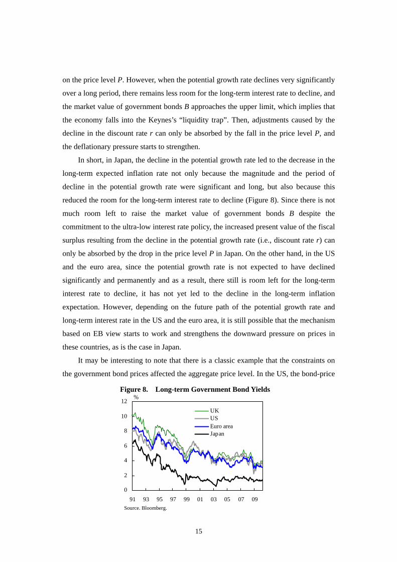
on the price level P. However, when the potential growth rate declines very significantly
over a long period, there remains less room for the long-term interest rate to decline, and
the market value of government bonds B approaches the upper limit, which implies that
the economy falls into the Keynes’s “liquidity trap”. Then, adjustments caused by the
decline in the discount rate r can only be absorbed by the fall in the price level P, and
the deflationary pressure starts to strengthen.
In short, in Japan, the decline in the potential growth rate led to the decrease in the
long-term expected inflation rate not only because the magnitude and the period of
decline in the potential growth rate were significant and long, but also because this
reduced the room for the long-term interest rate to decline (Figure 8). Since there is not
much room left to raise the market value of government bonds B despite the
commitment to the ultra-low interest rate policy, the increased present value of the fiscal
surplus resulting from the decline in the potential growth rate (i.e., discount rate r) can
only be absorbed by the drop in the price level P in Japan. On the other hand, in the US
and the euro area, since the potential growth rate is not expected to have declined
significantly and permanently and as a result, there still is room left for the long-term
interest rate to decline, it has not yet led to the decline in the long-term inflation
expectation. However, depending on the future path of the potential growth rate and
long-term interest rate in the US and the euro area, it is still possible that the mechanism
based on EB view starts to work and strengthens the downward pressure on prices in
these countries, as is the case in Japan.
It may be interesting to note that there is a classic example that the constraints on
the government bond prices affected the aggregate price level. In the US, the bond-price
Figure 8. Long-term Government Bond Yields
Source. Bloomberg.
0
2
4
6
8
10
12
91 93 95 97 99 01 03 05 07 09
UKUSEuro areaJapan
%
16
support program was adopted during the period from 1942 to 1951. In this period,
changes in the discounted present value of the fiscal surplus S/r resulted in fluctuations
in the price level P because the Federal Reserve used monetary policy to maintain the
market value of government bonds B. See the BOX for details.
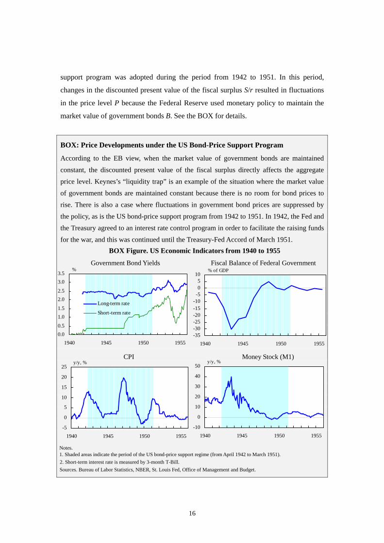
BOX: Price Developments under the US Bond-Price Support Program
According to the EB view, when the market value of government bonds are maintained
constant, the discounted present value of the fiscal surplus directly affects the aggregate price level. Keynes’s “liquidity trap” is an example of the situation where the market value of government bonds are maintained constant because there is no room for bond prices to rise. There is also a case where fluctuations in government bond prices are suppressed by the policy, as is the US bond-price support program from 1942 to 1951. In 1942, the Fed and the Treasury agreed to an interest rate control program in order to facilitate the raising funds for the war, and this was continued until the Treasury-Fed Accord of March 1951.
BOX Figure. US Economic Indicators from 1940 to 1955
Government Bond Yields Fiscal Balance of Federal Government
CPI Money Stock (M1)
Notes. 1. Shaded areas indicate the period of the US bond-price support regime (from April 1942 to March 1951). 2. Short-term interest rate is measured by 3-month T-Bill. Sources. Bureau of Labor Statistics, NBER, St. Louis Fed, Office of Management and Budget.
0.00.5
1.01.5
2.02.5
3.03.5
1940 1945 1950 1955
Long-term rate
Short-term rate
-35-30-25-20-15-10-505
10
1940 1945 1950 1955
% % of GDP
-5
0
5
10
15
20
25
1940 1945 1950 1955
-10
0
10
20
30
40
50
1940 1945 1950 1955
y/y, % y/y, %
17
Under the bond-price support regime, fiscal development clearly had a significant impact on the course of inflation.13 As shown in BOX figure, the CPI inflation rate was stable until 1946 due to wage and price controls, but surged toward 1948 after the price control was lifted. This price surge may be related with the fiscal deterioration (i.e., contraction of fiscal surplus S) during wartime, which instilled the private sector’s expectation that the government’s deteriorated fiscal condition would continue in the future. The decrease in the discounted present value of the fiscal surplus caused the wealth effect for the private sector, and then the private sector increased the selling pressure on government bonds in order to increase its expenditures. However, since the Fed maintained government bond prices constant, the selling pressure did not end. In other words, because the price of government bonds was maintained at a high level, the private sector with increased wealth continued to sell government bonds to increase its expenditures. As a result, the aggregate price level rose so that the real value of government bonds declined and finally it became commensurate with the present value of the fiscal surplus.
Then, deflation progressed over the period 1948-1950. This corresponds to the period in which the large wartime deficits had ended, and the US government budget was instead in surplus. Deflation resulted from the increase in the discounted present value of fiscal surplus under the bond-price support regime. And, with regard to the subsequent resurgence of inflation toward 1951, when the Korean War broke out, it was anticipated that the fiscal deficit would increase again, which seems to have served as inflationary pressure.
Japan’s Fiscal Conditions and the EB View
In this paper, in order to simplify our explanation about the EB view, fiscal surplus S is
assumed to be constant. Some may point out that this is an unrealistic assumption given
the fiscal conditions in Japan after the bursting of the bubble, where the fiscal deficit
expanded and the government debts went on increasing. However, even if the fiscal
surplus S is assumed to be variable, it does not change the main mechanism of the EB
view. What is important in the EB view is the discounted present value of the fiscal
surplus and not the fiscal surplus for the current period. Even when the current fiscal
deficit expands as the tax revenue declines as a result of a recession, the discounted
present value of the fiscal surplus may remain unchanged if the private sector expect
that the future tax will increase by as much as the increase in the fiscal deficit this
13 See Woodford (2001) for details.

18
year.14 On the contrary, the discounted present value of the fiscal surplus increases, if
the private sector expects that the real output growth rate will decline permanently and
as a result the discount rate r decreases. This then strengthens the downward pressure on
the price level. As is obvious from a simple calculation, a few percentage-point drop in
the discount rate r has the effect of multiplying the discounted present value of the fiscal
surplus.15 For this reason, even if the government debt B increases, as is the case in
Japan, downward pressures on the price level P may occur when the present value of the
fiscal surplus S/r has significantly increased due to the decrease in the discount rate r.
Sluggish Consumption and Increased Demand for Government Bonds
The EB view gives us a hint about the reason that sovereign risk has not emerged in
Japan to date despite the massive government debt. As a result of the decline in growth
expectations and the increase in the expected fiscal burden of the private sector, the
private sector’s savings (i.e., its demand for government bonds) increased sufficiently.
This helped the government bonds to be almost absorbed by domestic investors and kept
14 From the perspective of the EB view, whether fiscal policy affects the price level depends on whether the discounted present value of the fiscal surplus changes or not. An increase in the fiscal deficit does not have any impact on the price level unless the discounted present value of the fiscal surplus changes. 15 All other conditions being equal, for example, a permanent reduction in the discount rate r from 4% to 1% has the effect of increasing the discounted present value of the fiscal surplus by four times, and pushing down the price level considerably.
Figure 9. Investment-Saving Balances in Japan
Note. IS balance to GDP ratios. Source. Bank of Japan, “Flow of Funds”.
-15
-10
-5
0
5
10
15
80 82 84 86 88 90 92 94 96 98 00 02 04 06 08Corporate Sector General GovernmentHousehold Sector IS balance
Saving deficit
% of nominal GDP
FY
Saving surplus
19
the sovereign risk low.
In Japan, the household net saving rate has been on a decreasing trend since the
1990s (Figure 9), but this mainly results from the population aging and does not
necessarily suggest that individual households reduced their savings and increased
consumption expenditures. In reality, since the household sector as a whole suppressed
consumption, the aggregate demand slowed down and the business fixed investment did
not grow so much. As a result, net savings of the private sector, sum of the corporate
and the household sectors, increased from mid 1990s to around 2003, and financial
institutions increased the purchase of government bonds because of the decrease in
lending to the private sector.
7. Conclusion There is a positive cross-country correlation between adjusted money growth and
inflation (Figure 1), because the quantity equation of money (MV = PY) holds in both
the Money view and the EB view, and changes in velocity (ΔV) may not differ much
across countries. On the other hand, while the government’s inter-temporal budget
constraint (B/P = S/r) is also satisfied in both views, a positive cross-country correlation
between output growth (related to the discount rate r) and change in the price level P is
not observed (Figure 3). This is because the market value of government bonds B and
fiscal surplus S differ significantly across countries.
It is not appropriate to explain Japan’s price fluctuations by a single view, i.e.,
either the Money view or the EB view. The disinflation period during the 1990s, the first
half of the 1990s in particular, overlaps the period of sluggish growth of money due to
the decline in bank lending, which is consistent with the Money view. However, a strong
positive correlation between the long-term inflation expectation and the potential growth
is observed in Japan, which is not consistent with the Money view. From the perspective
of the EB view, growth expectations (and hence the potential growth rate) need to be
raised in order to overcome Japan’s deflation.16 If growth expectations of Japan’s
16 As well as the improvement in growth expectations (i.e., the increase in the discount rate r), the permanent reduction in fiscal surplus S decreases the present value of the fiscal surplus (S/r) and dispels deflationary pressures. However, it is very difficult for the government to credibly commit to reducing fiscal surplus S permanently, because Japan’s outstanding debt-GDP ratio is the worst among industrialized nations. That is, against the backdrop of the government’s deteriorated fiscal
20
economy improve, the expenditures of the private sector will increase, and the aggregate
price level will reverse to an upward trend. The Bank of Japan recently introduced the
fund-provisioning measure to support strengthening the foundations for economic
growth. This aimed to improve growth expectations and overcome deflation.
References
Bank of Japan “The Role of the Money Stock in Conducting Monetary Policy,” Bank of Japan Quarterly Bulletin, May2003.
Christiano, Lawrence J. and Terry J. Fitzgerald, “Price Stability: Is a Tough Central Bank Enough?,” Economic Commentary, Federal Reserve Bank of Cleveland, 2000a.
Christiano, Lawrence J. and Terry J. Fitzgerald, “Understanding the Fiscal Theory of the Price Level,” Economic Review, 36(2), Federal Reserve Bank of Cleveland, 2000b.
Cochrane, John H., “Money as Stock: Price Level Determination with No Money Demand,” NBER Working Paper, No.7498, 2000.
Leeper, Eric M., “Equilibria under Active and Passive Monetary and Fiscal Policies,” Journal of Monetary Economics, 27, 1991.
Sims, Christopher A., “The Precarious Fiscal Foundations of EMU,” De Economist, 147, No.4, 1999.
Woodford, Michael, “Control of the Public Debt: A Requirement for Price Stability?,” NBER Working Paper, No.5684, 1996.
Woodford, Michael, “Fiscal Requirements for Price Stability,” Journal of Money, Credit and Banking, 33, 2001.
condition, the private sector probably expects that tax will be raised in the future by just the same amount as the current increase in the fiscal deficit, and hence the discounted present value of fiscal burdens is not lessened and deflationary pressures is not dispelled. In addition, as seen in Greece, if reduction in fiscal surplus S is considered to be a lack of fiscal discipline by market participants, the market value of government bonds B will decline as a result of growing selling pressure on bonds, which then weakens the upward pressure on the price level.