The Role of Investability Restrictions on Size, Value, and Momentum in International Stock Returns

by

G. Andrew Karolyi and Ying Wu*

Abstract

Using monthly returns for over 37,000 stocks from 46 developed and emerging market countries over a two-decade period, we test whether empirical asset pricing models capture the size, value, and momentum patterns in international stock returns. We propose and test a multi-factor model that includes factor-mimicking portfolios (FMPs) based on firm characteristics and that builds separate FMPs comprised of globally-accessible stocks, which we call “global factors,” and only locally-accessible stocks, which we call “local factors.” Our new “hybrid” multi-factor model with both global and local factors not only captures strong common variation in global stock returns, but also achieves low pricing errors and rejection rates using conventional testing procedures for a variety of regional and global test asset portfolios formed on size, value, and momentum. First Version: November 23, 2011. This Version: February 1, 2012. Key words: International asset pricing; investment restrictions; cross-listed stocks. JEL Classification Codes: F30, G11, G15. * Karolyi is Professor of Finance and Economics and Alumni Chair in Asset Management at the Johnson Graduate School of Management, Cornell University and Wu is a Ph.D. student, Department of Economics, Cornell University. We are grateful for detailed comments from Ken French, for useful conversations with Vihang Errunza, Gene Fama, John Griffin, Kewei Hou, Bong-Chan Kho, Paolo Pasquariello, Richard Roll, René Stulz, Harry Turtle, and Cornell’s Finance Brown Bag Workshop participants and financial support from the Alumni Professorship in Asset Management at Cornell University. All remaining errors are our own. Address correspondence to: G. Andrew Karolyi, Johnson Graduate School of Management, Cornell University, Ithaca, NY 14853-6201, U.S.A. Phone: (607) 255-2153, Fax:(607) 254-4590, E-mail: gak56@cornell.edu

1

I. Introduction

Whether securities are priced locally in segmented markets or globally in a single integrated

market is an enduring question in international asset pricing, and one that has been reviewed by Karolyi

and Stulz (2003). The liberalization of financial markets around the world has increased market

accessibility for global investors, but many indirect barriers, such as political risk, differences in

information quality, legal protections for private investors and market regulations, can still inhibit full

market integration.

Early empirical tests focused on whether market or consumption risks are priced locally or

globally, following predictions made by the seminal international asset pricing models of Solnik (1974),

Grauer, Litzenberger and Stehle (1976), Sercu (1980), Stulz (1981), and Errunza and Losq (1985). In the

past decade, however, focus has shifted to the role of firm characteristics, such as size, book-to-market-

equity ratios, cash-flow-to-price ratios, and momentum, in pricing securities in global markets. And an

important debate has emerged over whether the explanatory power of these characteristics arises locally

or globally. Griffin (2002) studies a global variant of the three-factor model similar to that of Fama and

French (1993, 1998), which includes a market factor, a size factor and a book-to-market-equity factor for

four countries (U.S., U.K., Canada, and Japan). He finds that only the local, country-specific components

of the global factors are able to explain the time-series variations in the stock returns and multi-factor

models built from local factors only generally outperform those built from global factors with lower

pricing errors. These findings are important because other studies advocate for models that incorporate

both local and foreign components of factors based on firm characteristics (Bekaert, Hodrick, and Zhang,

2009).

The debate has further advanced with newer, more broad-based evidence in two recent studies.

Hou, Karolyi, and Kho (HKK, 2011) examine the relative performance of global, local, and what they call

“international” versions of various multifactor models to explain the returns of industry and

characteristics-sorted test portfolios in each country. The international versions of their models represent a

“hybrid” factor structure that includes separately local, country-specific factors as well as foreign factors

2

built from stocks outside the country of interest. They find that the international versions of these

multifactor models have much lower pricing errors than the purely local and global versions.1 They

recommend that the foreign components of these factors are as important as local components for pricing

global stocks. Fama and French (2011), however, show that a global multi-factor model performs only

passably for average returns on global size/book-to-market ratios (“B/M” hereafter) and size/momentum

portfolios, and it works poorly when asked to explain average returns on regional (for North America,

Europe, Japan, Asia-Pacific) size/B/M or size/momentum portfolios. They test hybrid models following

the methods in Griffin (2002) and HKK (2011) but find that the improved performance in terms of

explanatory power and lower pricing errors over the strictly local versions of the model (for which they

deem the performance only passable) is negligible.

In this paper, we make an important contribution to this debate. We propose and test a new multi-

factor model based on firm characteristics that builds separate factor portfolios comprised of only

globally-accessible stocks, which we call “global factors,” and only locally-accessible stocks, which we

call “local factors.” Our new “hybrid” multi-factor model with both global and local factors not only

captures strong common variation in global stock returns, but also achieves low pricing errors and

rejection rates using conventional testing procedures for a variety of regional and global test asset

portfolios formed on size, value, and momentum. Relative to a purely global factor model for global test

asset portfolios, the increase in explanatory power is substantial and the reduction in average absolute

pricing errors can be large; these gains are even larger for tests that include microcap stocks, that focus on

global test asset portfolios that exclude North America and that include a momentum factor in the model.

Relative to purely local factor models for regional test asset portfolios, the pricing errors and model

rejection rates for the hybrid model are similar, except for emerging market test asset portfolios for which

the hybrid model’s pricing errors and rejection rates are much lower.

1 HKK (2011) also show that the international version of their proposed multifactor model with the market factor, a

value factor constructed from cash-flow-to-price ratios, and a momentum factor (following Jegadeesh and Titman, 1993; Rouwenhorst, 1998; Griffin, Ji, and Martin, 2003; and, Asness, Moskowitz, and Pedersen, 2009) provides the lowest average pricing error and rejection rates among various versions of competing multifactor models.

3

Our experiment examines monthly returns for over 37,000 stocks from 46 countries over a two-

decade period. The intuition for this novel multi-factor structure comes from international asset pricing

models that account for barriers to international investment and from the empirical studies that validate

them.2 In particular, Errunza and Losq (1985) define a two-country world with two sets of securities: all

securities traded in the “foreign” market are eligible for investment by all investors (“globally

accessible”), but those traded in the “domestic” market are ineligible and can only be held by domestic

investors (“locally accessible”). These restrictions define the expected return on one of the ineligible

securities as a function of a global market risk premium (i.e., a global CAPM) plus a “super risk premium”

which is proportional to the conditional local market risk. The condition under which local market risk is

priced depends on the availability of substitute assets that may offer the same diversification opportunities

as with the ineligible securities. The model can reduce to the two polar cases of full integration or full

segmentation and, most importantly, allows for intermediate cases in between so that both global and

local risks can be priced. Though this model is derived in the context of the CAPM, we seek to extend the

same intuition (without formal theoretical justification) to extra-market factors based on firm-specific

attributes like size, value and momentum.

How we define the set of globally-accessible (“eligible”) and locally-accessible (“ineligible”)

stocks is critical for our exercise. Accessibility, or investability, refers to the ability of global investors to

access certain markets and securities in those markets, so any definition should include consideration of

openness (limits on foreign equity holdings), as well as perhaps liquidity, size, and float at the market and

individual security level. We choose to define globally-accessible stocks in our equity universe as those

that have shares secondarily cross-listed on at least one market outside of their main listing in their

country of domicile. Locally-accessible stocks are, therefore, those that are traded only in their respective

home markets. Again, our inspiration for this particular experimental choice comes from extensive

2 Among many others, we include Stulz (1981), Errunza and Losq (1985), Eun and Janakiramanan (1986), Bodurtha

(1999), Chaieb and Errunza (2007), and Errunza and Ta (2011), and extensive empirical evidence in Bekaert and Harvey (1995), Errunza, Hogan, and Hung (1999), de Jong and de Roon (2005), Carrieri, Errunza, and Hogan (2007), and Pukthuanthong and Roll (2009), and Bekaert, Harvey, Lundblad, and Siegel (2011).

4

research on risk and return attributes and institutional features of internationally cross-listed stocks.3

Some studies (Foerster and Karolyi, 1999; Errunza and Miller, 2000) show that the systematic risk

exposures of these stocks change dramatically and permanently around their secondary listings: local

market betas (measured relative to local market proxies) decline and foreign market betas (measured

relative to global market proxies) rise. Newly globally accessible, these cross-listed stocks are much more

likely to be held and traded by institutional investors in the U.S. and around the world (Ferreira and

Matos, 2008).

In our hybrid multi-factor model, global factor portfolios for the market, size, value and

momentum are constructed from globally-accessible stocks that are not only secondarily cross-listed but

also actively traded on exchanges outside of their home markets, while local factor portfolios for the

market, size, value and momentum are constructed only from locally-accessible stocks that are listed and

traded only in their home markets.4 The locally-accessible stocks are constructed from among the stocks

that are not globally accessible in the region in which our model is seeking to explain the cross-section of

average returns. That is, the local factors include only those stocks that are listed and traded in their home

markets. This is different from the construction of factors for the international models in Griffin (2002),

HKK (2011), as we reassign what would be local stocks in their local factors to the global factors if those

stocks are deemed globally accessible by our definition.

There are, of course, other ways in which stocks can become globally accessible, such as being

included in a closed-end country fund, or in one of Morgan Stanley Capital International (MSCI) or

Standard & Poor’s (S&P) global indexes (especially, in their investable indexes for emerging markets).

Indeed, if they do not face insurmountable or costly foreign investment restrictions that preclude them

3 Consider, among many others, studies by Alexander, Eun, and Janakiramanan (1988), Foerster and Karolyi (1993,

1999), Bodurtha (1994), Errunza, Hogan, and Hung (1999), Errunza and Miller (2000), Bekaert, Harvey, and Lumsdaine (2002), Doidge, Karolyi, and Stulz (2004), Carrieri, Errunza, and Hogan (2007), and Carrieri, Chaieb, and Errunza (2011). Karolyi (2006) provides a survey of the cross-listing literature.

4 We will define the globally accessible set to include stocks that secondarily cross-list their shares on one of seven different target markets: the U.S. on one of the major exchanges, New York Stock Exchange (NYSE), American Stock Exchange (AMEX) or Nasdaq, or on the over-the-counter (OTC) markets), the U.K. on the London Stock Exchange, London OTC, or SEAQ International, Euronext Europe, Germany, Luxembourg, Singapore, or Hong Kong. We later discuss the rationale behind this set of target markets.

5

from doing so, many institutions do hold shares of foreign stocks in their home markets even if they are

not secondarily cross-listed elsewhere. Though narrow in its definition, we prefer to consider only

secondary cross-listings for our globally-accessible set because of the clear identification of the listing

event as well as its timing. We also explore the robustness of our findings to several alternative

definitions of global accessibility, such as additional restrictions that account for how actively the cross-

listed shares are traded.

Our paper differs in scope from that of Fama and French (2011) in that we incorporate into our

analysis more than 11,000 stocks from 23 emerging markets. In fact, we include the emerging markets as

one of the regions in which we evaluate how well our hybrid multi-factor model performs for size, value,

and momentum test asset portfolios. Expanding our analysis into emerging markets is important because

it is there that investability restrictions are most likely to bind. We expect that this is where a global or

hybrid model is likely to face the greater challenge relative to a purely-local factor model. Like Fama and

French (2011), we provide evidence for size groups. Our sample, like theirs, covers all size groups, and

indeed very small, microcap stocks produce challenging results (Fama and French, 2008). We control for

the potential influence of microcap stocks globally and in each region by performing our tests with and

without the extremely-small test asset portfolios and also by building the factor portfolios using value and

momentum breakpoints using the top 90% of market capitalization in each region to limit their influence.

Section II outlines the experiment. Section III describes our global equity universe, the globally-

accessible and locally-accessible sets, and furnishes summary statistics. The construction of the factor

portfolios and test assets are outlined in Section IV and our main results follow in Section V. Section VI

describes several robustness tests and Section VII concludes the paper.

II. The Design of the Experiment

To examine the role of investability restrictions on the size, value, and momentum patterns in

international stock returns, this study begins with an investigation of firm-level characteristics of

6

individual stocks from all 46 countries over our full 22-year sample, from 1989 to 2010. Specifically, we

seek to answer the following important questions:

(1) Does accounting for investability restrictions improve the explanatory power of the global factor

model for cross-sectional and time-series variation in global and regional stock returns?

(2) How robust is the explanatory power of the proposed new “hybrid” model to alternative

definitions for the globally accessible sample?

(3) How robust is the explanatory power of the proposed new “hybrid” model to using different

numbers of factors and different test assets?

Fama and French (1993) propose a three-factor model to capture the patterns in U.S. average

returns associated with size and value versus growth,

Rit – Rft = αi + βi (Rmt – Rft) + si FSize,t + hi FB/M,t + εi,t (1)

In this regression, Rit is the return on asset i in month t, Rf is the risk free rate, Rmt is the market return,

FSize,t is the difference between the returns of diversified portfolios of small stocks and big stocks (F

denotes a factor portfolio), and FB/M,t is the difference between the returns on diversified portfolios of high

B/M (value) stocks and low B/M (growth) stocks. Model (1) is motivated by observed patterns in returns

and the authors (Fama and French), as well as those of us who follow their lead, readily acknowledge that

they try to capture the cross-section of expected returns without specifying the underlying economic

model that governs asset pricing. The null hypothesis is that the slope coefficients (𝛽𝑖, si, hi) and the

associated factor portfolio returns capture the cross-section of returns, so we test whether the intercepts

equal zero for all test assets. This test is akin to the mean-variance spanning tests of Huberman and

Kandel (1987). For a given set of test asset portfolios, we judge each model based on its explanatory

power, the magnitude of model pricing errors (the absolute magnitude of the intercepts), and the Gibbons,

Ross, and Shanken (GRS, 1989) F-test statistic for the hypothesis that the intercepts are jointly equal to

zero across the test assets of interest. We also follow Lewellen, Nagel, and Shanken (2010) by computing

a core component of the GRS statistic, denoted SR(α),

SR(α) = [α’S-1α]1/2 (2)

7

where α is the vector of regression intercepts produced by Model (1) across a set of test asset portfolios. S

is the covariance matrix of regression residuals.5

Fama and French (2011) build the global and local versions of model (1) for global and local

stock returns respectively:

Rit – Rft = αGi + βG

i (RGmt – Rft) + sG

i FGSize,t + hG

i FGB/M,t + εi,t (3a)

Rit – Rft = αLi + βL

i (RLmt – Rft) + sL

i FLSize,t + hL

i FLB/M,t + εi,t (3b)

for which the superscript “G” on the market and factor portfolios implies that they are constructed from

all stocks around the world and the superscript designation of “L” on the market and factor portfolios

implies that they are constructed only from local - or regional, in our experiments - stocks. Extending the

experiment in this way is naturally complicated by the fact that asset pricing globally or even in a

particular region may not be fully integrated.

To capture the impact of investability restrictions on global investing, we propose a new hybrid

model based on the Fama-French three-factor model,

Rit – Rft = αHi + βCL

i (RCLmt – Rft) + sCL

i FCLSize,t + hCL

i FCLB/M,t

+ βNCLi (RNCL

mt – Rft) + sNCLi FNCL

Size,t + hNCLi FNCL

B/M,t + εi,t (4)

where the superscript “H” denotes the intercept for the hybrid model, the superscript “CL” denotes a

market or factor portfolio comprised of stocks only in the globally-accessible sample, which is

represented by the sample of secondary cross-listings (CL) in this study, and the superscript “NCL”

denotes a market or factor portfolio comprised of the purely-local stocks from the specific region (those

not secondarily cross-listed overseas) for which the test is performed.

Our second experiment examines whether the empirical validity of the hybrid model is influenced

by the purely mechanical way in which we construct the globally-accessible and purely-local subsamples.

We adjust the investment opportunity set by gradually imposing a variety of “viability constraints” on the

5 Gibbons, Ross, and Shanken (1989) relate SR(α)2 to the difference between the square of the maximum Sharpe

ratio for the portfolios constructed from the test asset portfolios and factor portfolios and that constructed from the factor portfolios alone. As Fama and French (2011) argue, the advantage of this statistic is that it combines the regression intercepts with a measure of their precision captured by the covariance matrix of the regression residuals.

8

globally accessible sample. That is, we require that the stocks in the globally accessible sample qualify by

meeting certain minimum thresholds of trading volume in the target markets for the secondary cross-

listing. In comparing the performance of the hybrid model in which the global factors are built in different

ways, we still find reliable evidence about the explanatory power of the hybrid model in explaining

returns in both global and regional test asset portfolios.

In our third and final experiment, we investigate whether the cross-sectional explanatory power of

the hybrid model is specific to the Fama-French three-factor model in explaining the portfolios sorts on

size and B/M. Carhart (1997) proposes a four-factor model for U.S. return in order to capture momentum,

Rit – Rft = αi + βi (Rmt – Rft) + si FSize,t + hi FB/M,t + mi FMom,t + εi,t (5)

which is Model (1) enhanced with a momentum return, FMom,t is the difference between the month t

returns on a diversified portfolios of the winners and losers of the past year. Similarly, we test a hybrid

model based on the Carhart’s four-factor model,

Rit – Rft = αHi + βCL

i (RCLmt – Rft) + sCL

i FCLSize,t + hCL

i FCLB/M,t + mCL

i FCLMom,t

+ βNCLi (RNCL

mt – Rft) + sNCLi FNCL

Size,t + hNCLi FNCL

B/M,t + mNCLi FNCL

Mom,t + εi,t (6)

which is Model (4) extended by two momentum factor portfolio returns, FCLMom,t, the difference between

the month t returns on diversified portfolios of the winners and losers of the past year from the globally

accessible sample (the cross-listed stocks in our study), and FNCLMom,t is the difference between the month

t returns on diversified portfolios of the winners and losers of the past year from the purely local sample

from the specific region for which the test is performed (the non-cross-listed stocks in our study).

III. Data and Summary Statistics

A. The Global Equity Universe

We obtain international stock returns and accounting data from Datastream and Worldscope. To

ensure that we have a reasonable number of firm-level observations in each country, the sample period

begins in November 1989 and ends in December 2010, which encompasses the widest coverage in the

Worldscope database. Our final sample of the global equity universe includes 37,399 stocks from 46

9

countries. To ensure that there are sufficient numbers of stocks in each test asset portfolio, as in Fama and

French (2011), 23 developed markets are combined into four regions: (i) North America (NA), including

the U.S. and Canada; (ii) Japan; (iii) Asia Pacific, including Australia, New Zealand, Hong Kong, and

Singapore (but not Japan); and (iv) Europe, including Austria, Belgium, Denmark, Finland, France,

Germany, Greece, Ireland, Italy, the Netherlands, Norway, Portugal, Spain, Sweden, Switzerland, and the

U.K. And the remaining 23 countries are combined into Emerging Markets, the fifth region in our tests; it

includes Israel, Turkey, Pakistan, South Africa, Czech Republic, Poland, Hungary, Russia, China, India,

Indonesia, Malaysia, Philippines, South Korea, Taiwan, Thailand, Argentina, Brazil, Chile, Colombia,

Mexico, Peru, and Venezuela.

Market integration within one region is important for the power of our asset pricing tests. The U.S.

and Canada share the world’s largest and most comprehensive trading relationships for goods and

securities. Close economic, legal, and political linkages have been established among the countries of

Europe. Some evidence of segmentation and fracturing of these linkages abounds, but market integration

is a reasonable working assumption in North America and Europe, and therefore improves the precision

of the tests for these regions. On the other hand, it is unlikely that the countries in the Emerging Markets,

or those in Asia Pacific, are close to one market during our sample period. Low market integration in

these two regions may cause problems of large average absolute intercepts and poor regression model fit

in the tests. Our results suggest that the hybrid model provides a better description of average returns for

portfolios formed on size and value (or size and momentum) in the regions where these countries are

partially segmented.

We require each firm’s home country to be clearly identified in the database. Financial firms are

excluded from the study due to their different characteristics. We also exclude depositary receipts (DRs),

real estate investment trusts (REITs), preferred stocks, and other stocks with special features.6 For most

6 We drop stocks with name including “REIT”, “REAL EST”, “GDR”, “PF”, “PREF”, or “PRF” as these terms may

represent REITs, GDRs, or preferred stocks. We drop stocks with name including “ADS”, “CERTIFICATES”, “RESPT”, “Rights”, “Paid in”, “UNIT”, “INCOME FD”, “INCOME FUND”, “HIGH INCOME”, “INC.&GROWTH”, “INC.&GW”, “UTS”, “RTS”, “CAP.SHS”, “SBVTG”, “STG.SAS”, “GW.FD”, “RTN.INC”,

10

countries, we restrict the sample to stocks from major exchanges, which we define as the exchanges on

which the majority of stocks in that country are listed. However, multiple exchanges are included in

samples for China (Shanghai Stock Exchange and Shenzhen Stock Exchange), Japan (Osaka Stock

Exchange, Tokyo Stock Exchange, and JASDAQ), Russia (MICEX and Russian Trading System), South

Korea (Korea Stock Exchange and KOSDAQ), Canada (Toronto Stock Exchange and TSX Ventures

Exchange), and the U.S.(NYSE, AMEX and NASDAQ). To limit the effect of survivorship bias, we

include dead stocks in the sample.

To reduce errors in Datastream, we follow several screening procedures for monthly returns as

suggested by Ince and Porter (2003) and HKK (2011). First, any return above 300% that is reversed

within one month is set to missing. Specifically, if Rt or Rt-1 is greater than 300%, and if (1+ Rt) × (1+ Rt-1)

- 1 ≤ 50%, then both Rt and Rt-1 are set to missing. Second, in order to exclude remaining outliers in

returns that cannot be identified as stock splits or mergers, we treat as missing the monthly returns that

fall out of the 0.1% and 99.9% percentile ranges in each country. Third, included firms are required to

have at least 12 monthly returns during the sample period.

Additionally, we require the availability of the following financial variables for at least one firm-

year observation: market value of equity (“Size” hereafter), B/M, and cash flow to price (“C/P” hereafter).

To make sure that the accounting ratios are known before the returns, we match the financial statement

data for fiscal year-end in year t-1 with monthly returns from July of year t to June of year t+1. We take

the inverse of the price-to-book ratio (WC09304) and the price-to-cash flow ratio (WC09604) to calculate

the ratios of B/M and C/P, respectively. We do not use negative B/M (or C/P) stocks when calculating the

breakpoints for B/M (or C/P) or when forming the size/B/M (or size/C/P) portfolios.

Figure 1 exhibits the distribution of our global equity universe across regions over the period

from 1990 to 2010, reported by total market capitalization. On average, North America, Europe, Japan,

Asia Pacific, and the Emerging Markets account for 43.13%, 25.50%, 13.44%, 4.45%, and 13.49% of

“VCT”, “ORTF”, “HI.YIELD”, “GUERNSEY”, “DUPLICATE”, “DUAL PURPOSES”, and “NOT Rank for Dividend” due to various special features. A number of additional country-specific screening rules are applied.

11

global market capitalization. Figure 2 offers a slightly different picture based on the total number of

stocks. North America constitutes one-quarter of the sample population, higher than Europe (23.08%),

Japan (11.50%), and Asia Pacific (10.47%) but lower than the Emerging Markets (29.72%).

Proportionally more large-cap stocks are concentrated in North America, especially the U.S. In contrast,

proportionally more of the stocks from Asia Pacific and Emerging Markets are small cap stocks. In

addition, Figures 1 and 2 show the distribution of our global equity universe across countries within each

region. Among the countries in Europe, the average size of stocks in the Netherlands, Spain, and

Switzerland are larger than those in Greece, Sweden, and the U.K. Hong Kong accounts for 40.62% of all

market capitalization in Asia Pacific but only constitutes 24.96% of the sample population in the region.

Most of the stocks in Emerging Markets are from Asia, either by count or by total market capitalization.

The average size of stocks varies substantially across emerging market countries, with greater values for

Mexico, Brazil, Russia, and China.

Figure 3 shows the sample over time and breaks it down by regions. There are some differences

in the evolution of counts and total market capitalization. The counts steadily increase from around

10,000 in 1990 to a peak of almost 28,000 in 2008. Especially, the count in Emerging Markets has

jumped from less than 2,000 in 1990 to nearly 9,500 in 2009. In contrast to these counts, global market

capitalization has less steady growth. It rises from US$7 trillion in 1990 to a peak of US$26 trillion in

2000. It falls after 2000 before reaching another peak of almost US$40 trillion in 2007. In the most recent

two years, it rises again to reach US$34 trillion in 2010.

Table 1 presents summary statistics of total counts, global betas, country betas, and other firm-

level characteristics for each country. We compute betas with respect to the value-weighted global and

country portfolios to which a stock belongs. These betas are estimated annually for each stock at the end

of June of each year, using its previous 36 monthly returns (12 months minimum). The median global

betas range from an average of 1.27 for Singapore to 0.12 for Colombia. The country betas are

measurably larger than the global betas. In addition to the betas, Table 1 reports the time-series averages

of median size, B/M, C/P, and momentum (“Mom” hereafter). There is considerable cross-country

12

variation in the average median B/M, but much less for C/P. Mom for month t is the cumulative return for

t-11 to t-1, skipping the sort month t. The first momentum sort absorbs one year of data, so the sample

period for Mom is November 1990 through December 2010. Among all the countries in our sample, Mom

ranges from a low of -2.19% (Japan) to highs of 40.97% (Poland), 37.17% (Russia), and 26.48% (China).

B. The Globally Accessible Sample and Purely Local Sample of Stocks

In our hybrid model, global factors are constructed from the set of globally accessible stocks and

local factors are constructed from the set of purely local stocks from the region where the experiment is

performed. We categorize stocks into two subsets based on accessibility or investability constraints as

defined by whether or not the stock is secondarily cross-listed on an overseas stock market in addition to

its primary listing in the home market and whether that secondary cross-listing is associated with a

minimum level of trading activity. Ultimately, we identify a set of around 5,400 stocks accessible to

global investors by being cross-listed in major developed markets; another group of more than 32,000

individual stocks are locally accessible to domestic investors. We acknowledge that previous studies have

used global industry portfolios, closed-end country funds, and the investable indices in emerging markets

as globally-accessible assets used to replicate returns on only locally accessible assets (e.g., Bekaert and

Urias, 1996; Carrieri, Chaieb and Errunza, 2008, 2011; Errunza and Ta, 2011). In this study, we focus on

the impact of the secondary cross-listing on the size, value, and momentum patterns in international stock

returns to keep the accessibility criteria as transparent as possible.

We require that the stocks in the globally accessible sample need to be cross-listed in at least one

of several outside target markets beyond their home country. Within those select target markets, we

include secondary listings from overseas that can trade on many different venues or platforms. We

confine the list to seven target markets: (i) the U.S., which includes NYSE/AMEX, NASDAQ, and the

Non-NASDAQ OTC markets;7 (ii) the U.K., which includes the London Stock Exchange, London OTC

7 Non-Nasdaq OTC markets include both the OTC Bulletin Board, an interdealer electronic quotation system and the

OTC Markets Group, for which its OTCQX International trading platform is designed for secondary listings from overseas.

13

Exchange, London Plus Market, and SEAQ International; 8 (iii) Europe, which includes Euronext at

Amsterdam, Brussels, Lisbon, Paris, and EASDAQ; 9 (iv) Germany in which the Frankfurt Stock

Exchange is located; (v) Luxembourg in which the Luxembourg Stock Exchange is located; (vi)

Singapore, which includes the Singapore Stock Exchange, Singapore OTC Capital, and Singapore

Catalist;10 and (vii) Hong Kong in which the Hong Kong Stock Exchange is located. The distinguishing

feature of these target exchanges is that they are fully open to global investors, having minimum foreign

investment restrictions and reasonably active trading in foreign cross-listed issues. We try to strike a

balance between obtaining maximum breadth of stock exchange platforms accessible for international

investors and avoiding problems related to differences in cross-listing trading mechanisms and

conventions. For the Frankfurt Stock Exchange, for example, there are “unregulated” cross-listed stocks

alongside the “regulated” cross-listed stocks, in which trading takes place without the sponsorship of the

company.11 We include both unregulated and regulated cross-listings in Frankfurt.

The appendix describes the procedure for constructing the sample of globally accessible stocks.

Our sample construction begins with all non-domestic stocks listed in the target exchanges. If one firm is

only listed on an exchange in its home market, the firm is excluded from this sample. We drop stocks

denominated with a currency other than that of the host market,12 stocks whose records of investment type

8 The London Plus Stock Exchange (www.plusmarketsgroup.com) is a London-based stock exchange providing cash

trading and listing services and regulated under the auspices of the Markets in Financial Instruments Directive (2004/39/EC, “MiFiD”), a European Union (EU) law providing for harmonized investment services in the EU. London OTC trading falls under the auspices of the London Stock Exchange (LSE) Group (www.londonstockexchangegroup.com) and is done under MiFiD with the exchange furnishing trade reporting and publication services. The Stock Exchange Automated Quotation (SEAQ) International is the LSE’s electronic price quotations system for non-U.K. securities.

9 EASDAQ was an electronic securities exchange based in Brussels founded originally as an equivalent to Nasdaq in the U.S., was purchased by the American Stock Exchange in 2001 and then shut down in 2003.

10 See www.sgx.com for details on main board versus Catalist listing requirements. Like the Alternative Investment Market in the U.K., a listing applicant must be sponsored by an approved sponsor of Catalist and must satisfy some disclosure and performance requirements. Singapore’s OTC Capital (www.otccapital.com) is an unaffiliated trading platform for shares of unlisted public companies.

11 If a company is already listed on an approved foreign stock exchange (“Like Exchanges”), it is exempt from the primary registration rules and can be dual listed on the Frankfurt Stock Exchange without an underwriter. There are over 200 such “Like Exchanges” approved by the Frankfurt Stock Exchange (www.franfurtstockexchange.de). Given the looser regulation on the Frankfurt Exchange unregulated program, we perform a robustness check to assure that the inclusion of the Frankfurt Stock Exchange does not affect our results.

12 This exclusion criterion affects only stocks in the U.S., Singapore and Hong Kong.

14

are not clearly identified in the database, and those recorded as instrument types other than ADRs, GDRs,

or equity in the database.

From the list containing over 30,000 stocks, we select those with available records of home

market and a parent code in the database so that the cross-listed stocks in the target exchanges can be

matched with their parent stocks listed in the home market. Because there are a few mismatches in

Datastream, we verify the matching records. We correct the mismatched records for the cross-listed

stocks if their true parent equities can be found in the global universe sample, keep those that have no

parent equities but are only listed on the target exchanges, and drop those whose true parent equities are

missing in the database. To ensure the validity of the sample, we drop the stocks whose Return Index (RI)

records are not available in the database.13 Furthermore, if one stock is cross-listed on more than one

target exchange within the same target market, these multiple records are consolidated into one record.

The sample at this point contains 22,612 stocks. Similar to the global equity universe, we exclude

financial firms and confine the sample to firms from 46 countries. Included stocks are required to have

available company account items from Worldscope, and the parent stocks need to have at least 12

monthly RI records during the sample period. After these filters, there are totally 11,051 stocks, and the

sample is labeled as “CL1” to denote the first group of cross-listed stocks.

To construct our final sample, we impose additional restrictions on how actively the secondarily

cross-listed shares are traded, which we call our “viability” constraints. We only drop the cross-listed

stocks for which trading in the target markets is too limited to be viably accessible for global investors.

For each stock in CL1, we compare (a) its monthly trading in the target markets with the total trading of

all secondarily cross-listed stocks from the same country (using VA, turnover by value, from Datastream)

and (b) its monthly trading volume (VO, turnover by volume, from Datastream) in the target markets

13 To limit the effect of survivorship bias, we include dead stocks in the sample. For both dead and active stocks, we

confirm their effective ending months according to two criteria: (i) consecutive constant RIs from the month until the end of the period, December 2010; and, (ii) zero trading volume from the month until the end of the period. If one stock has the same month for its base month and ending month, the stock is excluded from the sample.

15

relative to that of the same stock in the home market.14 The first viability constraint evaluates the annual

percentage of its trading in target markets relative to all secondarily cross-listed stocks from the same

country trading there. If the time-series average of the annual percentages during the sample period is

required to be at least 0.5%, there are nearly 900 stocks that qualify, many of which are the most

popularly traded stocks for global investors. For the stocks that fail to meet our first viability criterion, we

use a second one based on the annual percentage of its own global trading volume in any of the target

markets (Baruch, Karolyi, & Lemmon, 2007). If the time-series average of these annual percentages

during the sample period is required to be at least 0.1%, there are around 5,300 stocks left in the sample.

Merging these two globally accessible sets yields 5,439 stocks, which we call the "Main CL Sample."

Figure 4 presents its distribution across regions over the period from 1990 to 2010, reported by

total market capitalization. On average, North America (35.97%) and Europe (32.82%) constitutes the

bulk of the total market capitalization in the Main CL Sample, followed by Japan (14.38%), the Emerging

Markets (11.64%), and Asia Pacific (5.19%). Relative to their stake in the market capitalization of the

global equity universe (Figure 1), North American cross-listed stocks are relatively under-represented. By

count, North America, Europe, Japan, Asia Pacific, and Emerging Markets represent 42.97%, 23.75%,

3.62%, 14.43%, and 15.22% of the sample population respectively (shown in Figure 5). The average sizes

of the cross-listed stocks in the U.S., Europe, and Japan are larger than those in Canada and Asia Pacific.

Relative to their stake in the count of stocks in the global equity universe (Figure 2), Canadian and Asia-

Pacific cross-listed stocks are significantly over-represented. We can rightly infer that the market

capitalization of Canadian and Asia-Pacific cross-listed stocks are smaller than those from elsewhere.

Overall, there is considerable dispersion within and across home market regions in size among the

globally-accessible stocks.

14 Trading volume in the target markets is adjusted by the bundling ratio (or ADR ratio, recorded as the Exchange

Ratio from Datastream). Each ADR (or GDR) represents a specific number of shares that are immobilized in the home market by the depositary bank’s custodian. Bundling ratios for direct listings are implicitly equal to one since the same share trades in the target market as in the home market.

16

Figures 4 and 5 also exhibit the distribution of Main CL Sample stocks across countries within

each region. In Europe, stocks from France, Germany, the Netherlands, and Switzerland are more likely

to have shares secondarily cross-listed overseas but stocks from Austria, Greece, and the U.K. tend to stay

in their home markets. In Asia Pacific, Hong Kong stocks are over-represented in the Main CL Sample

relative to the global equity universe. Among emerging market countries, equities from China, India, and

Taiwan are more likely to stay at home. On the other hand, equities from Russia, Mexico, and South

Africa tend to go abroad.

Figure 6 illustrates the total market capitalization and the total number of the globally accessible

sample, represented by the Main CL Sample, and breaks them down by regions and by year. Total count

increases from less than 1,000 in the early 1990s to a peak of 3,856 in 2008. It falls for two years after

2008 to reach 3,756 in 2010. Among the five regions, the count from North America has increased 14.36

times from 1990 to 2010 and it is the only region that keeps rising in count for the most recent two years.

In contrast to the counts, total market capitalization, as well as the market capitalizations from each region,

has experienced more volatility over the period, reaching peaks in 2000 and 2007 (almost US$18 trillion).

Figure 6 also shows the distribution of Main CL stocks by each target market and by year. Most

notably, the U.S. as a target market for internationally cross-listed stocks is more resilient than those in

the U.K., Europe, and Germany, either by count or by market capitalization. Annual counts in the U.K.

reach a peak of 600 in 2007 and decrease steadily to 250 in 2010. For Europe, the number of cross-listed

stocks never goes up above 440 and it decreases steadily from 437 in 2001 to 263 in 2010. For the

Frankfurt Stock Exchange, the annual count increases significantly from less than 250 in the early 1990s

to 2,885 in 2008, but it falls during the most recent two years until down to 2,788 in 2010. Distinct from

these markets, NYSE/AMEX, Nasdaq and the Non-Nasdaq OTC markets have attracted more foreign

stocks cross-listed. Even after the 2008 financial crisis, the count is steadily rising from 1,746 in 2007 to

2,137 in 2010 (Iliev, Miller, and Roth, 2011). Although all target markets have shrunk in size around

2008, the market capitalization in the U.S. drops by 20.98% from 2007 to 2009, much less than the 75.95%

in the U.K., 42.71% in Europe, and 29.15% in Germany.

17

In addition to the Main CL Sample, we construct and evaluate three other definitions for the

globally accessible sample, together with CL1, to ensure the reliability of the hybrid model we propose.

First, we consider our second viability constraint alone: Each stock in the sample is required to have at

least 0.1% of annual global trading volume taken place in any of the target markets on average during the

sample period. The resulting sample has 5,311 stocks and is labeled “CL2a.” Second, we introduce an

absolute viability constraint: for each stock in CL1 in a given year, if there is at least one month of non-

zero trading in the target markets, the stock is included in the globally accessible sample for that year.

Another new sample, denoted “CL2b,” then contains 9,579 stocks. Because of potential concerns about

the fact that still a few large stocks in the major target markets (such as the U.S.) are excluded from the

globally-accessible set by our viability constraints, we add stocks which are in the top 50% of total market

capitalization from each target exchange, to the Main CL Sample, which we denote “CL2c.” For each

globally accessible sample, we group the stocks left in each respective region as the purely local sample.

Summary statistics, including total counts, global betas, country betas, and other firm-level characteristics,

for the Main CL Sample and its counterparts are provided in Appendix Tables 1 and 2.15

IV. Building Factor Portfolios and Test Assets

We follow Fama and French (1993, 2011) in constructing proxy factors as returns on zero-

investment portfolios that go long in stocks with high values of a characteristic and short in stocks with

low values of the characteristic. These factors are explanatory returns in our asset pricing regression

models. We also follow Fama and French (2011) in constructing 5×5 size/B/M portfolios, the 5×5

size/momentum portfolios, and the 5×5 size/C/P portfolios that are used as test assets in our tests.

A. Building Factor Portfolios

Our first asset pricing tests are for 5×5 size/B/M portfolios and the explanatory returns are for

2×3 portfolios sorted on size and B/M. As in Fama and French (2011), at the end of each June from 1990

to 2010, we allocate stocks in one region to two size groups – small stocks and big stocks. Big stocks are

15 These appendix tables as well as all others mentioned below are available upon request.

18

those in the top 90% of market capitalization for the region, and small stocks are those in the bottom 10%.

The only difference between our sorting breakpoints and those of Fama and French (2011) is related to

the B/M breakpoints. Fama and French (2011) uses the 30th and 70th percentiles of B/M for the big stocks

in each given region to avoid undo weight on micro-cap stocks. However, there are still differences in

terms of accounting rule across countries within any one region, especially Europe, Asia Pacific, and the

Emerging Markets. Given the fact that our globally accessible stocks are more likely to accept

International Financial Reporting Standards (IFRS) or global standards for reporting that can be

comparable across countries within the region, we follow the line of reasoning in Fama and French (2011)

and use the B/M breakpoints based on the big stocks in the globally accessible sample from each region to

avoid sorts that are dominated by the less comparable and tiny stocks in the region.

The global explanatory returns are constructed from the globally accessible sample. Similar to

Fama and French (2011) in constructing the global portfolios, we use a universal size breakpoint, but use

each region’s B/M breakpoints to allocate the globally accessible stocks. The size factor, SMB, is then the

equally-weighted average of the returns on three small stock portfolios minus the equally-weighted

average of the returns on three big stock portfolios. And the value factor, HML, is the equally-weighted

average of the returns on two value stock portfolios minus the equally-weighted average of the returns on

two growth stock portfolios. Beyond the global returns, the hybrid model includes local explanatory

returns that are based on the purely local stocks from the region for which the test is performed. Fama and

French (2008, 2011) document that microcap stocks pose a challenge for asset pricing models and suggest

factor returns should not be dominated by small stocks. Small stocks constitute the major component of

the purely local samples. So, if the size breakpoint is the bottom 10th percentile of market capitalization of

the purely local sample for each region, either the size factor or the value factor will be dominated by

small stocks. Thus we follow Fama and French (2011) and use regional size cutoffs for the purely local

portfolios. In addition, we adopt the same regional B/M breaks as in the globally accessible portfolios to

avoid the microcap effect.

19

Another set of explanatory returns are 2×3 factor portfolios returns sorted on size and momentum,

which will be introduced in our second asset pricing tests on size/momentum portfolios. The momentum

factor, WML, is formed following Fama and French (1998, 2011) using a 12-month/2-month strategy

where each month’s return is the average return on the two high prior return portfolios minus the average

return on the two low prior return portfolios. Similar to the size/B/M portfolios, the momentum

breakpoints for the global explanatory returns are the 30th and 70th percentiles for the big stocks in the

globally accessible sample from each region. And we use the regional momentum cutoffs based on big

stocks for the given region when forming local explanatory returns. As in Fama and French (2011), the

momentum breakpoints from each region are employed in forming global portfolios. In our third set of

tests on size/C/P portfolios, we build the set of explanatory returns that are for 2×3 portfolios sorted on

size and C/P. The explanatory return associated with C/P is constructed by the same way as HML.

Table 2 presents summary statistics for factor portfolios returns. Among the global test asset

portfolios in Panel A, the global market premium, a respectable 0.46% per month, is 1.59 standard errors

from zero over the sample period. The market premium of the Developed Markets portfolios is similar to

the global market premium. For either the Global portfolios excluding North America or the Developed

Markets portfolios excluding North America, the market premium drops to as low as around 0.33% per

month. Among the five regional test asset portfolios in Panel B, Japan aside, the market premiums are

higher in all three of the developed regions than in the Emerging Markets. Within developed markets,

Asia Pacific stands out, with an average equity premium of 0.74% per month, followed by North America

(0.68%), Europe (0.58%), and Japan (-0.04%). As usual, the estimates of market premiums are imprecise,

especially in Emerging Markets with a t-statistic of only 0.79 and Japan, only -0.10. We find similar

results for size and value premiums as in Fama and French (2011). There is no size premium in the global

and regional test asset portfolios. And there are value premiums everywhere. Premiums on C/P are

generally higher than premiums on B/M for all the global and most of the regional test asset portfolios.

In addition, Table 2 illustrates the difference in factor returns between the globally accessible

sample and the purely local sample, for each global and regional experiment. Market premiums are higher

20

for the globally accessible samples than the purely local stocks in most of the regions except North

America. In the global portfolios, the size premiums for the globally accessible samples are higher than

those for the purely local samples because of the differences in the size distributions of globally

accessible samples and purely local samples, ranging from 0.42% for the Global portfolios excluding

North America to 0.36% for the Developed Markets portfolios. The estimates are usually beyond the two

standard-error bound. The purely local sample has a higher value premium than the globally accessible

sample everywhere. Because small stocks are more plentiful in the purely local sample, their

fundamentals are typically more dispersed. As for momentum returns, the globally accessible sample in

North America is conspicuously up to 1.33% per month (t = 2.75), higher than the premium for the purely

local sample, 0.42% (t = 1.47).To save space, we report the correlations of factor portfolio returns in

Appendix Tables 3 and 4.

B. Building Test Assets

The test assets in our first asset pricing tests are 5×5 size/B/M portfolios and we follow the

method in Fama and French (2011). The size breakpoints for a region are the 3rd, 7th, 13th, and 25th

percentiles of the region’s aggregate market capitalization. The B/M breakpoints are defined by the 20th,

40th, 60th, and 80th percentiles for big stocks in the region. Table 3 displays the average excess returns for

the 5×5 size/B/M. Our results confirm the finding in Fama and French (2011) that the size pattern in value

premiums poses a challenge for asset pricing models. The next two test assets are 5×5 size/momentum

portfolios and 5×5 size/C/P portfolios. For the sake of brevity, average excess returns for these two types

of test asset portfolios are reported in Appendix Tables 5 and 6.

V. Time-Series Regression Tests

Our first experiment involves time-series regression tests, as applied by Fama and French (1993,

1996, and 2011) and others, in which test assets are 5×5 size/B/M portfolios. We compare the

performance of global, local, and hybrid versions of the Fama-French three-factor model. Our criteria for

success consist of the explanatory power (average adjusted R2 across the test asset portfolios), the GRS

21

statistic, the Sharpe Ratio, SR(𝛼), and summary statistics for the intercepts, including the difference

between the highest and lowest regression intercepts (“H-L α”) and the average absolute intercepts (“|α|”).

A. Main Experiment

Table 4 reports regressions to explain excess returns on the 5×5 portfolios from the sorts on size

and B/M. Appendix Tables 7 and 8 furnish details on the intercepts and their t-statistics, as well as the

betas for the hybrid model based on the Fama-French three-factor model. Panel A of Table 4 summarizes

the results for the global version of the Fama-French three-factor model. The global factor model offers

adequate explanatory power for the global test asset portfolios, but fares poorly for the returns on regional

size/B/M test asset portfolios. The average R2 is 0.92 for the global portfolios, but it is lower (only 0.83) if

North America is excluded. Among the five regional tests asset portfolios, the average R2 reaches only as

high of 0.72 for Europe and is as low as 0.32 for Japan. The GRS statistics for the Global portfolios (3.12

and 2.67, for Developed Markets only) are well into the right tail of the relevant F-distribution and the

average absolute intercepts average 0.16% per month. Part of the reason for the model rejections may

arise from the poor explanatory power of the regressions, as we see that the GRS statistics for the Global

portfolios without North America are much lower (1.27 overall, 1.58 for Developed Markets only). For

the regional test asset portfolios, however, we have not only poor explanatory power, but also high GRS

statistics beyond the 99th percentile of the F-distribution (except for Japan and the Emerging Markets).

Another possible reason for the high model rejection rates is the presence of extremely small stocks. In a

separate part of Panel A, we also present the same statistics for only the 4×5 global test asset portfolios,

excluding the five in the smallest size quintile. There is modest improvement in average R2 but the GRS

statistics and their Sharpe ratio (SR(α)) core components are much lower.

Panel B of Table 4 reports results for the regressions of the purely local factor model in

explaining excess returns on just the five regional test asset portfolios. Consistent with Fama and French

(2011), our results indicate that the local three-factor model works well in Japan and Europe. Despite the

fact that the GRS tests reject North America and Asia Pacific at the 99th percentile of the F-distribution,

the purely local factor model performs better than the purely global factor model in all experiments,

22

pushing up the average R2s and lowering the average absolute intercepts. The microcap stocks in North

America are still a challenge for the models; the GRS statistic without them is only 1.57, but then it rises

to 2.12, microcap stocks included, which would constitute a rejection at the 99% level. For Emerging

Markets, the purely local factor model works well if only judged by the GRS test. However, without a

presumption of integrated pricing in the region, the power loss is significant with an average R2 of only

0.65. The poor performance of the purely local factor model makes it unattractive for an application for

which the focus is on emerging markets.

To now, we have re-established many of the key inferences from Fama and French (2011) for the

three-factor model. Panel C of Table 4 now illustrates the results of the new hybrid version of the Fama-

French three-factor model. The hybrid model works distinctly better than the purely global factor model

for global test asset portfolios. All the average R2s are pushed up to over 0.89 or even higher, with and

without microcap stocks. The average absolute intercepts for all the five global test asset portfolios are

0.11% or less, microcap stocks aside, and 0.13% or less, microcap stocks included. The Sharpe ratios,

SR(α), for the intercepts shrink for all four of the experiments. Consider, for example, that for the Global

portfolios, the GRS statistic falls from 3.12 for the purely global factor model to 1.73 for the hybrid

model. Excluding the microcap stocks, the hybrid model achieves yet a smaller GRS statistic, 1.08, below

the 90th percentile of the relevant F-distribution. For the Developed Markets portfolios, shifting to the

hybrid model pushes the average R2 from 0.90 up to 0.95 without microcap stocks and from 0.89 to 0.94

with microcap stocks. It also lowers the average absolute intercepts to some extent and the GRS statistics.

Appendix Table 7 illustrates that the only three remaining statistically significant intercepts all fall within

the set of the smallest five quintile portfolios.

The improved performance from the hybrid model is more notable when we turn to the

regressions on the Global portfolios excluding North America and the Developed Markets portfolios

excluding North America. For the Global portfolios excluding North America, the hybrid model improves

upon the performance of the global factor model in explaining the average excess returns, lifting the

average R2s from 0.83 to 0.90 without microcap stocks and from 0.83 to 0.89 with microcap stocks,

23

shrinking the average absolute intercepts from 0.25% to 0.11% without microcap stocks and from 0.24%

to 0.13% with microcap stocks. In addition, the GRS statistics fall to 0.88 without microcap stocks and

1.17 with microcap stocks, and neither of them leads to the rejection for the null hypothesis. The hybrid

model produces an even greater improvement over the purely global factor model when it is asked to

explain the average returns on the Developed Markets portfolios excluding North America. When

microcap stocks are dropped, the average R2 rises from 0.78 for the global factor model to 0.94 for the

hybrid model, the average absolute intercept drops from 0.35% to 0.07%, the Sharpe ratio falls from 0.38

to 0.29, and the GRS is only 0.82. Even with microcap stocks, the hybrid model still performs well,

improving on the purely global factor model by any of the evaluation criteria. In sum, the hybrid model is

quite successful in capturing average returns on global portfolios.

For the regional test asset portfolios, the hybrid model and the purely local factor model produce

similar regression fits. In North America, Europe, Asia Pacific, and Japan, the average absolute intercepts

for the hybrid model are close to those for the purely local factor model, and there are no significant

differences in terms of the Sharpe ratio and the GRS statistic. In the Emerging Markets test, however, the

hybrid model works better than the purely local factor model in shrinking the average absolute intercepts.

Without microcap stocks, the average absolute intercept for the purely local factor model is 0.42%, which

is much higher than that for the hybrid model of 0.13%. With microcap stocks, if the purely local factor

model is replaced by the hybrid model, the average absolute intercept falls by more than half, from 0.43%

to 0.19%. The superior performance of the hybrid model in the Emerging Markets is likely due to the

hybrid model’s introduction of an important feature: the dependence of emerging markets on developed

markets. Indeed, in Appendix Table 8, the betas for the test asset portfolios in the Emerging Markets on

the market, size, and value factor portfolios for the globally-accessible set are economically large and

statistically important.

B. Robustness Checks

We further test the reliability of the hybrid model by carrying out two rounds of robustness

checks. We first check the hybrid versions of the Fama-French three-factor model which are built on

24

other definitions of the globally-accessible sample. A second round of tests involves time-series

regressions to see whether the inclusion of the Frankfurt Stock Exchange – and especially its large

number of unsponsored secondary foreign listings - in the list of target exchanges changes the results.

Table 5 summarizes regressions to explain excess returns on size/B/M portfolios when the Main

CL Sample is replaced by four alternative definitions of the globally-accessible set of stocks. We first

disregard the so-called viability constraints and start with the largest globally accessible sample, denoted

CL1. Recall that this sample represents 91% of the global market capitalization, so we expect this

experiment is most likely to inhibit the performance of the hybrid model relative to the local models for

regional portfolios. Panel A of Table 5 shows that for all four global test asset portfolios, the tight

regression fits affirm that the hybrid model is economically meaningful, and the GRS test indicates that

using CL1 for the hybrid model works as well as using the Main CL Sample. Taking the Global portfolios

as an example, without microcap stocks, the GRS statistic is 1.14 for the hybrid model built on CL1,

slightly higher than 1.08 for that built on the Main CL Sample. With microcap stocks, the GRS statistic,

1.88, is also close to 1.73. However, as distinguished from the tests using our Main CL Sample, the

benefit of using CL1 in the global experiments comes at the cost of the relatively poorer regression fits for

the regional test asset portfolios, especially those for North America and Europe. Microcap stocks aside,

for the North America test, the hybrid model produces a higher GRS statistic, 2.03, which is above the

99th percentile of the F-distribution. In Europe, the GRS statistic rises as high as 1.78. The problems

(witnessed by higher GRS statistics, higher average absolute intercepts, and larger Sharpe ratios) result

from the weaker local factors in the two regions. The purely local sample in North America or Europe

accounts for less than 10% of total market capitalization of the region.

Part B of Table 5 reports the regression results when CL2a is used. This more stringent relative

viability constraint (consider own trading only and require above 0.1% of global trading volume occurs in

target cross-listing markets) shrinks the globally accessible sample, and in particular the U.S. companies

that are viably accessible by the new definition are pushed down to account for only 18% of the total

market capitalization in the U.S.. In the regional experiments, the hybrid model works just as well as the

25

purely local factor model in North America, Europe, Asia Pacific, and Japan. With smaller average

absolute intercepts and higher average R2, the hybrid model performs much better than the purely local

factor model and somewhat better than the hybrid model with the Main CL sample in the Emerging

Markets tests. In the global experiments, throwing more stocks, mostly from the U.S. by size, out of the

globally accessible sample increases the contribution of global factors in explaining the Global portfolios

excluding North America and the Developed Markets portfolios excluding North America. For instance,

in the test on the Global portfolios excluding North America, the new CL2a sample produces ever smaller

Sharpe ratios for the intercepts: 0.28 without microcap stocks and 0.37 with microcap stocks.

Additionally the GRS statistics are usually lower than 1.10, which is below the 90th percentile of the F-

distribution. However, if North America is added into the global test asset portfolios, microcap stocks

aside, the GRS statistics increase up to 1.40 for the Global portfolios and 1.50 for the Developed Markets

portfolios.

Panel C of Table 5 reports the results for the hybrid model built on what we call “CL2b.”

Changing from relative viability constraints (at least 0.1% of global trading volume occurs in target

markets or at least 0.5% of total trading value in target markets relative to all secondarily cross-listed

stocks from the same country trading there ) to an absolute viability constraint (at least one month in the

past year with non-zero trading volume in a target cross-listing market) does not affect the performance of

the hybrid model in explaining the average returns for global test asset portfolios and most of the regional

test asset portfolios. The North America sample is the only exception in which the hybrid model now has

a power problem, possibly because the absolute viability constraint breaks the consistency of our time-

series explanatory returns: some companies are identified as purely local stocks when there are no

overseas trading records but as globally accessible stocks when trading actually occurs in the target

markets. Switching these companies between the two samples may alter the profile of the returns of the

explanatory factor portfolios. And this distortion becomes even more severe when these companies are

large in size. This is exactly what happens in the U.S.: Exxon Mobil, Apple Inc., Microsoft Corporation,

Wal-Mart Stores and other popularly-held large cap stocks are only in CL2b for some years.

26

Panels D of Table 5 presents the results when stocks in the top 50% of total market capitalization

from each target exchange are added into the Main CL Sample. The new sample, CL2c, when compared

with the Main CL Sample, has the same sets of globally accessible stocks from Japan (accounting for 54%

of the total market capitalization in Japan) and the Emerging Markets (44%), slightly larger sets from

Europe (70%) and Asia Pacific (61%), and larger set from North America (65%). As a result, the hybrid

model makes even more improvements than those where the Main CL Sample is used for global test asset

portfolios. For example, for the Global portfolios, the GRS statistics fall from 1.08 to 0.98 without

microcap stocks and from 1.73 to a 1.50 with microcap stocks, which cannot be rejected at the 95% level.

For the Developed Markets portfolios, the GRS statistics decline from 1.34 to 1.22 without microcap

stocks, and from 2.45 to 2.04 with microcap stocks. The new hybrid model performs similarly to that

when the Main CL Sample is used for regional test asset portfolios. The only difference is the North

America test. The GRS statistics jump up to 2.75 without microcap stocks and to 3.08 with microcap

stocks. If almost all large-cap U.S. stocks are placed in the globally-accessible set, the purely local sample

left in North America accounts for less than 40% of total market capitalization from the region. Because

most of the stocks in the purely local sample are small-cap stocks, it is harder for the local SMB factor to

fully reflect the size pattern in the local average returns. The significantly increased representation of

large-cap stocks in the global factors may also adversely affect the performance of this version of the

hybrid model since the representative investors for some large-cap stocks are still local investors inducing

noise from the misidentification. Both weak local factors and “noisy” global factors render this version of

the hybrid model unable to fit with the partially segmented market structure we seek.

What do we learn from this first round of robustness checks? The hybrid model appears quite

resilient in explaining the average returns in both the global and regional test asset portfolios. But it is

important to have sufficient numbers of stocks in factor portfolios. If a more stringent viability constraint

is imposed, the smaller size (either by count or by size) of the globally accessible sample will weaken the

representativeness of the global factors, thus making the cutoffs of B/M less appropriate. On the other

hand, although the hybrid model works better for the global test asset portfolios, when more stocks are

27

allowed into the globally accessible sample, the hybrid model becomes less attractive in explaining the

regional test asset portfolio returns due to smaller numbers of stocks left in the purely local sample.

Finally, adding all large-cap stocks from the target exchanges to the globally accessible sample does

improve the explanatory power of the hybrid model in the global tests. The failure in the North America

test confirms Fama and French (2011) that North America is a special case in the international asset

pricing tests. And our results suggest that imposing additional criteria, such as our two relative viable

constraints, on the large-cap stocks from the North America is needed to ensure that the marginal

investors for the globally accessible stocks are global investors, instead of local investors.

Given the looser secondary cross-listing rules on the Frankfurt Stock Exchange, we repeat the

experiments above for the case where the Frankfurt Stock Exchange is excluded from the list of target

exchanges. Our results are not driven by the inclusion of the Frankfurt Stock Exchange. To save space,

the regression results are only shown in Appendix Table 9. When no viability constraints are imposed on

this globally accessible sample, the hybrid model provides good descriptions for our four global test asset

portfolios. The GRS statistics are not higher than 1.08 without microcap stocks and not higher than 1.88

with microcap stocks. On the other hand, the hybrid model fares poorly in North America and Europe.

For example, in the North America test, the GRS statistics increase to 2.31 without microcap stocks and

to 2.77 with microcap stocks; the average absolute intercepts rise to 0.15% versus 0.11% for the purely

local factor model without microcap stocks, and 0.17% versus 0.14% for the purely local factor model

with microcap stocks. When the globally accessible sample is screened by our relative viability

constraints based on just six target markets without Germany, the hybrid model performs better than the

purely global factor model for the global test asset portfolios and works as well as the purely local factor

model for the regional test asset portfolios.

In sum, the hybrid model not only captures strong common variation in global and regional stock

returns, but also brings low pricing errors and rejection rates for a variety of regional and global test asset

portfolios. Compared with the purely global factor model for global test asset portfolios, the hybrid model

always achieves better performance: the explanatory power increases up to 0.89 or even higher, average

28

absolute pricing errors have reduced to 0.13% or even lower, the GRS statistics are not rejected at the 90%

level when microcap stocks are excluded. Compared with the purely local factor model for regional test

asset portfolios, the hybrid model brings neither larger pricing errors nor higher model rejection rates, and

it performs even better for Emerging Market test asset portfolios.

VI. More Robustness Tests

A. Time-series Regression Tests for Size/Momentum Portfolios

Table 6 summarizes the asset pricing tests in which the Carhart four-factor model is applied to

explain excess returns on 5×5 size/momentum portfolios. The Fama-French three-factor model generally

works poorly in such an experiment in terms of regression fit and GRS statistic (Fama and French, 2011,

their Tables 6 and 7). So, we turn to the Carhart (1997) four-factor model to build our hybrid model.

There are power problems with the global Carhart four-factor model for the global test asset

portfolios. Reasonable performance is only achieved in the Global portfolio tests when microcap stocks

are removed: the average R2 is 0.92, the average absolute intercept is 0.12%, and the GRS statistic is 1.89,

which is below the 99th percentile threshold. For the three other global test asset portfolios, the global

four-factor factor model fares poorly, producing higher GRS statistics and large average absolute

intercepts. For instance, for the Developed Markets portfolios, the GRS statistic is 2.05, which exceeds

the 99th threshold of the F-distribution, even without microcap stocks. The test on the Developed Markets

portfolios excluding North America has a relatively lower GRS statistic of 1.42, but this result is

hampered by low power. As with earlier results on size/B/M portfolios, the global factor model fares

poorly for the regional portfolio returns. By contrast, the local Carhart four-factor model is reasonable for

applications in the regional test asset portfolios for North America and Japan. The regressions on Europe,

Asia Pacific, and the Emerging Markets are relatively disappointing: even leaving microcap stocks aside,

the GRS test rejects the purely local factor model in these three regions.

The experiment for size/momentum portfolios produces the most disappointing results among all

asset pricing tests for the global or purely local versions of the Carhart model, as Fama and French (2011)

29

uncover. But, even with this challenge, the hybrid model fares reasonably well. For the Global portfolios,

the hybrid model and the global factor model perform similarly. In the three other global test asset

portfolios, the hybrid model better captures the returns than the global factor model. Using the Developed

Markets portfolios excluding North America as an example, we see the regression fit improves from 0.77

for the global factor model to 0.93 for the hybrid model. The average absolute intercepts fall from 0.32%

to 0.13% without microcap stocks and experience a similar decrease with microcap stocks. In the

regional tests, the hybrid model produces high GRS statistics in Europe (2.90 without microcap stocks),

Asia Pacific (2.25 without microcap stocks), and Emerging Markets (1.58 without microcap stocks), but

these are all similar to the results for the purely local factor model. The regression fits and the average

absolute intercepts are also close. The improvement of the hybrid model over the purely local factor

model arises in the Emerging Markets test asset portfolios: the average absolute intercepts decline from

0.60% to 0.38% without microcap stocks, and from 0.69% to 0.44% with microcap stocks.

Echoing previous robustness checks on size/B/M portfolios, we use four other globally accessible

samples to reconstruct the explanatory factor returns and get supporting evidence on the resilience of the

hybrid model (all shown in Appendix Table 10). Among all five cross-listed samples, CL2b (which

includes stocks with non-zero target market trading during the year) produces the lowest model rejection

rates for all four global test asset portfolios. Compared with the Main CL Sample in the regional

experiments, CL2b enlarges the average absolute intercepts from 0.15% to 0.18% without microcap

stocks and from 0.20% to 0.24% with microcap stocks in the North America test. In tests of other regions,

the performance of CL2b comes close to those of the Main CL Sample and CL2a (with one threshold

target trading level required). In addition, we are interested in whether the performance of the hybrid

model is driven by the inclusion of the unregulated cross-listing on the Frankfurt Stock Exchange.

Appendix Table 11 reports the regression results when the Frankfurt Stock Exchange is dropped from the

list of target exchanges. The results are quantitatively similar to those reported in Table 6.

30

Preliminary results show that the hybrid version of the HKK (2011) three-factor model performs

reasonably well for size/momentum portfolios. 16 We compare the Carhart four-factor model and the

extended version of the HKK (2011) three-factor model in which the SMB factor in Fama and French

(2011) is added. The HKK (2011) extended four-factor model is equivalent to the Carhart four-factor

model in explaining the average returns on the global and regional portfolios. Like the global Carhart

four-factor model, the global HKK (2011) extended four-factor model works well for the Global

portfolios when microcap stocks are dropped: the average R2 is 0.92, the average absolute intercept is

0.13%, and the GRS statistic is 1.88 (reported in Appendix Table 12). As before, for the three other global

test asset portfolios the global HKK (2011) extended four-factor model produces low power and large

average absolute intercepts. In the regional scenarios, the local HKK (2011) extended four-factor model

works well for North America and Japan, but suffers loss of power and higher model rejection rates for

Europe, Asia Pacific, and Emerging Markets. On the other hand, the hybrid version of the HKK (2011)

extended four-factor model increases the average R2 up to 88% and shrinks the average absolute

intercepts down to less than 0.18% in the global tests, and it does not fare worse than the local version in

the regional test asset portfolios.

We repeat previous robustness checks on size/momentum portfolios, including trying several

alternative definitions of global accessibility and dropping the unregulated cross-listed stocks that have

only been traded on the Frankfurt Stock Exchange. Once again, we uncover supporting evidence for the

hybrid model. For the sake the brevity, regression results are provided in Appendix Tables 12 and 13.

B. Time-series Regression Tests for Size/C/P Portfolios

Table 7 provides the regressions of the Carhart four-factor model in explaining excess returns on

size/C/P portfolios. As in Fama and French (2011), there is a size pattern in the average value premium in

the sorts on C/P, but it is somewhat weaker than the sorts on B/M. It is perhaps not surprising then that

the GRS statistics do not increase much when microcap stocks are considered. For example, if the global 16 HKK (2011) propose and test a three-factor model that includes the C/P and momentum FMPs in addition to the

global market portfolios and that produces the lowest pricing errors among various multifactor models in regressions for country, industry, and characteristic-sorted portfolios: Rit – Rft = αi + βi (Rmt – Rft) + ci FC/P,t + mi FMom,t + εi,t substitutes for Eqn. (1).

31

Carhart four-factor model is used in the test of the Global portfolios, the GRS statistics are 1.73 for the

4×5 portfolios and 1.96 for the 5×5 portfolios.

Panel C of Table 7 indicates that the hybrid model improves the regression fit of the global factor

model. Moreover, the average absolute intercepts drop to 0.12% and the GRS statistics are all below 1.53,

when microcap stocks are excluded. At the same time, the regressions of the hybrid model are largely

similar to those of the purely local factor model for the regional test asset portfolios. The GRS statistics,

average absolute intercepts, and SR(a) are close in the North America test. In addition, if the purely local

factor model is replaced by the hybrid model, excluding microcap stocks, the average absolute intercepts

decrease from 0.16% to 0.08% for Japan, and from 0.50% to 0.20% for the Emerging Markets. With

microcap stocks, the average absolute intercepts decrease from 0.14% to 0.09% for Japan, and from 0.51%

to 0.23% for the Emerging Markets. In the Europe test, the hybrid model fares slightly worse than the

purely local factor model. The average absolute intercept rises from 0.08% in the purely local factor

model to 0.14% in the hybrid model when microcap stocks are dropped. Despite that, the GRS test is not

rejected if evaluated at the 95th percentile of the F-distribution.

We perform three more robustness checks with the size/C/P test asset portfolios (as reported in

Appendix Tables 14 through 17). We first try alternative definitions for the globally-accessible sample for

the Carhart four-factor model; there are measurable benefits to extend the global factor model to the

hybrid model in most experiments. Second, we drop the cross-listed stocks from the Frankfurt Stock

Exchange and repeat the tests. Excluding them does not change the results. We also find that the hybrid

model maintains its performance when the global factors and local factors are adjusted by different

viability constraints and size considerations. Finally, we apply the HKK (2011) extended four-factor

model in the tests on the 5×5 size/C/P portfolios. The results are quantitatively similar to those in Table 7.

To conserve space, we report these results in Appendix Table 16. Our test does not permit us to

adequately distinguish the Carhart four-factor model and the HKK (2011) extended four-factor model

when it comes to explain the size/C/P portfolios. The HKK (2011) model is another reasonable choice for

applications in international asset pricing.

32

C. Time-series Regression Tests for Additional Portfolios and Individual Securities

In this section, we first build global test-asset portfolios that include just globally accessible

stocks. Intuitively, we expect many global asset managers would impose such accessibility constraints to

define their investment universe. In this setting, we further expect the traditional global factor model is

most likely to succeed, so we propose a test to compare the ability of the traditional global factor and our

new global factor model, in which the factor portfolios are built only from the globally accessible stocks,

to explain the portfolio returns. Here, we mainly check the experiments on the Global portfolios and the

Developed Markets portfolios.17

When compared to the traditional global factor model, the new global factor model yields lower

average absolute intercepts, lower Sharpe ratios, smaller GRS statistics and higher R2s. The results hold

for all three sets of 5×5 test asset portfolios sorted on size-B/M, size-momentum, and size-C/P. Taking the

size/B/M Developed Markets portfolios as an example, without microcap stocks, the average absolute

intercept falls from 0.20% for the traditional global factor model to 0.13% for the new global factor

model. With microcap stocks, average absolute intercept declines from 0.20% to 0.14%. In terms of

SR(a), the new global factor model produces smaller values: 0.35 without microcap stocks and 0.41 with

microcap stocks, compared to 0.40 and 0.44 respectively for the traditional global factor model.

Accompanied with similar or even tighter regression fits, the GRS statistics drop from 1.74 for the

traditional global factor model to 1.32 for the new global factor model, microcap stocks aside, and from

1.56 to 1.34, if microcap stocks are added. In either case we cannot reject at the 90% level. The complete

set of regression results is available in Appendix Tables 18.

We next move to supplementary tests using regressions on individual stocks to assess the

explanatory powers of the local factor model and the hybrid model for their returns. Each month,

beginning with November 1990, individual security regressions are estimated over 180 rolling 60-month

periods. The last period ends in December 2010. In all regions, the hybrid Fama-French three-factor

17 If North America is excluded in the global test asset portfolios, there are only 2,274 stocks for the Developed

Markets portfolios excluding North America and at most 3,100 stocks for the Global portfolios excluding North America. Technically, the numbers of stocks are insufficient to construct portfolios.

33

models achieve statistically significant increases in the average adjusted R2. The incremental R2s account

for, on average over time, 10.78%, 7.65%, 7.00%, 2.34%, and 17.53% of the R2s by the corresponding

local models in the North America, Europe, Asia Pacific, Japan, and Emerging Markets tests.

Interestingly, the increases in R2s for North America and Japan hit their peaks during the 2007-2008 crisis

period, while those for Europe, Asia Pacific and especially Emerging Markets reach their highest levels in

the late 1990s and early 2000s.

Furthermore, we decompose our hybrid model in order to evaluate the incremental R2 from

adding the global factors to the local factors. The global factors in the hybrid model increase the average

adjusted R2 by 2.10%, 1.22%, 1.04%, 0.73%, and 2.28% in North America, Europe, Asia Pacific, Japan,

and Emerging Markets, respectively. The increase in the average adjusted R2 due to the addition of global

factors can be expressed relative to the total average adjusted R2 for the hybrid model. The proportion of

the explained variance attributable to global factors is 13.88%, 6.86%, 5.25%, 2.07%, and 15.36% in

North America, Europe, Asia Pacific, Japan, and Emerging Markets, respectively, indicating the

importance of global factors in the hybrid model.

VII. Conclusions

Using monthly returns for over 37,000 stocks from 46 developed and emerging market countries

over a two-decade period, we test whether empirical asset pricing models capture the size, value, and

momentum patterns in international stock returns. We specifically propose and test a new multi-factor

model that includes factor-mimicking portfolios based on firm characteristics and that builds separate

ones comprised of globally-accessible stocks, which we call “global factors,” and only locally-accessible

stocks, which we call “local factors.” Our new hybrid multi-factor model with both global and local

factors not only captures strong common variation in global stock returns, but also achieves low pricing

errors and rejection rates using conventional testing procedures for a variety of regional and global test

asset portfolios formed on size, value, and momentum.

34

A critical ingredient of our analysis is how we categorize the equity universe into two subsets -

the globally-accessible sample and purely-local sample of stocks – based on accessibility or investability

constraints as defined by whether or not the stock is secondarily cross-listed on an overseas stock market

in addition to its primary listing in the home market and whether that secondary cross-listing is associated

with a minimum level of trading activity. To capture the impact of investability constraints on the size,

value, and momentum patterns in international stock returns, we then build separate factor portfolios –

global ones comprised stocks only in the globally-accessible sample, and local ones comprised of the

purely-local stocks from the specific region for which the test is perform – and propose a new “hybrid”

multifactor model. We find that neither a purely global factor model nor a purely local factor model can

work as well as the new “hybrid” when asked to explain average returns on global and regional size/value

and size/momentum portfolios. The new “hybrid” model does not encounter the problems of the purely

global factor models, such as high rates of rejections with GRS tests and large average absolute intercepts.

Rather, it improves the regression fit and reduces the pricing errors, with or without microcap stocks. And,

at the same time, the new “hybrid” model fares reasonably relative to a purely local factor model, and

works even better for emerging markets, in terms of explanatory power, model pricing errors and

rejection rates. The robustness of the new “hybrid” model is confirmed by tests made with a variety of

definitions of global accessibility, other double-sorted test portfolios, and other asset pricing models.

We interpret our findings in this study as a step forward in the international asset pricing literature

with important implications for practitioners in guiding cost-of-capital calculations and risk control and

performance evaluation analysis of global portfolios. Of course, we acknowledge several limitations in

the scope of our work as well as in the implementation. There may be alternative ways in which stocks

become globally accessible beyond secondarily cross-listing on overseas exchanges that we have not

considered. Including other mechanisms for global investor accessibility, such as being included in one of

MSCI or S&P global indexes (especially, in their investable indices in emerging markets), emerging

market ETFs and closed-end country funds, would be valuable to explore how the returns of global factor

portfolios have changed over time. We also cannot disregard the fact that simply being accessible does

35

not necessarily mean global investors will actually pursue these opportunities. Although this fact is taken

into consideration to a certain extent by imposing additional viability restrictions on how actively the

cross-listed shares are traded in our experiments, a more comprehensive picture of institutional trading

around the world would reveal the varying preferences and constraints face by different groups of

institutional investors. One would also hope for a more reliable proxy for the measure of viability

consideration than relative (and absolute) criteria in this study. Third, one could criticize our reliance on

conventional test procedures, which is necessarily limiting. Finally, it also remains to be seen whether the

new proposed “hybrid” model works for country, industry, and other characteristic-sorted test asset

portfolios, as evaluated in HKK (2011).

There are also other possible avenues for future work. We can study the effect of exchange rate

risks on the relative performance of global factors and local factors in the new “hybrid” model. All of our

returns are U.S. dollar denominated at prevailing exchange rates. Because the majority of investors are

different for globally accessible stocks and purely local stocks, the need to hedge exchange rates varies

and exchange rate risks are expected to play different roles in global factors and local factors. Exchange

risk is certainly a potential problem in global asset pricing. A key contribution of Solnik’s (1974)

influential international asset pricing model is that currency risk can be priced and there is also growing

evidence that the magnitude of currency-risk exposures can be quite large (Dumas and Solnik, 1995; De

Santis and Gerard, 1997, 1998; Griffin and Stulz, 2001). Second, we can extend the new “hybrid”

structure to incorporate the cross-sectional variations of currencies, commodities, and bonds, which

comprise a significant portion of global investment activity.

36

References

Alexander, G., C.S. Eun, and S. Janakiramanan, 1988, International Listings and Stock Returns: Some Empirical Evidence, Journal of Financial and Quantitative Analysis, 23, 135-151.

Asness, C.S., Tobias J. Moskowitz, and Lasse H. Pedersen, 2009, Value and Momentum Everywhere,

Working paper, National Bureau of Economic Research. Baruch, Samuel, G. Andrew Karolyi, and Michael L. Lemmon, 2007, Multimarket Trading and Liquidity:

Theory and Evidence, Journal of Finance, 62, 2169-2201. Bekaert, G., and C. Harvey, 1995, Time-varying World Market Integration, Journal of Finance, 50, 403-

444. Bekaert, G., C.R. Harvey, and R.L. Lumsdaine, 2002, Dating the Integration of World Equity Markets,

Journal of Financial Economics, 65, 203-248. Bekaert, G., C.R. Harvey, C.T. Lundblad, and S. Siegel, 2011, What Segments Equity Markets? Review

of Financial Studies, doi: 10.1093/rfs/hhr082. Bekaert, G., Robert J. Hodrick, and Xiaoyan Zhang, 2009, International Stock Return Comovements,

Journal of Finance, 64, 2591-2626. Bekaert, G., and M.S. Urias, 1996, Diversification, Integration and Emerging Market Closed-End Funds,

Journal of Finance, 51, 835-869. Bodurtha, J., 1994, International Factors and U.S. Equity Excess Returns, Working paper, Georgetown

University. Bodurtha, J., 1999, International Investment Restrictions and Factor Pricing, Working paper, Georgetown

University. Carhart, Mark M., 1997, On Persistence in Mutual Fund Performance, Journal of Finance, 52, 57-82. Carrieri, F., I. Chaieb, and V. Errunza, 2008, On the Pricing of Investable Securities and the Role of

Implicit Barriers, Working paper, McGill University. Carrieri, F., I. Chaieb, and V. Errunza, 2011, Do Implicit Barriers Matter for Globalization? Working

paper, Swiss Finance Institute Research Paper No. 10-55. Carrieri, F., Errunza, V., and K. Hogan, 2007, Characterizing World Market Integration Through Time,

Journal of Financial and Quantitative Analysis, 42, 915-940. Chaieb, I., and V. Errunza, 2007, International Asset Pricing Under Segmentation and PPP Deviations,

Journal of Financial Economics, 86, 543-578. De Jong, F., and F. A. De Roon, 2005, Time-varying Market Integration and Expected Returns in

Emerging Markets, Journal of Financial Economics, 78, 583-613. De Santis, Giorgio, and Bruno Gerard, 1997, International Asset Pricing and Portfolio Diversification

with Time-Varying Risk, Journal of Finance, 52, 1881-1912.

37

De Santis, Giorgio, and Bruno Gerard, 1998, How Big Is the Premium For Currency Risk? Journal of

Financial Economics, 49, 375-412. Doidge, Craig, G. Andrew Karolyi, and Rene M. Stulz, 2004, Why Are Foreign Firms Listed in the U.S.

Worth More? Journal of Financial Economics, 71, 205-238. Dumas, Bernard, and Bruno Solnik, 1995, The World Price of Foreign Exchange Risk, Journal of

Finance, 50, 445-479. Errunza, V., and D. Miller, 2000, Market Segmentation and the Cost of Capital in International Equity

Markets, Journal of Financial and Quantitative Analysis, 35, 577-600. Errunza, V., and E. Losq, 1985, International Asset Pricing under Mild Segmentation: Theory and Test,

Journal of Finance, 40, 105-124. Errunza, V., and H. Ta, 2011, The Impact of Investability on Asset Valuation, Working paper, McGill

University Errunza, V., K. Hogan, and M.W. Hung, 1999, Can the Gains from International Diversification be

Achieved without Trading Abroad? Journal of Finance, 54, 2075-2107. Eun, C. S., and S. Janakiramanan, 1986, A Model of International Asset Pricing with a Constraint on the

Foreign Equity Ownership, Journal of Finance, 41, 897-914. Fama, Eugene F., and Kenneth R. French, 1993, Common Risk Factors in the Returns on Stocks and

Bonds, Journal of Financial Economics, 33, 3-56. Fama, Eugene F., and Kenneth R. French, 1996, Multifactor Explanations of Asset Pricing Anomalies,

Journal of Finance, 51, 55-84. Fama, Eugene F., and Kenneth R. French, 1998, Value versus Growth: The International Evidence,

Journal of Finance, 53, 1975-1999. Fama, Eugene F., and Kenneth R. French, 2008, Dissecting Anomalies, Journal of Finance, 63, 1653-

1678. Fama, Eugene F., and Kenneth R. French, 2011, Size, Value, and Momentum in International Stock

Returns, Working paper, University of Chicago. Ferreira, Miguel A., and Pedro Matos, 2008, The Colors of Investors’ Money: The Role of Institutional

Investors Around the World? Journal of Financial Economics, 88, 499-533. Foerster, S.R., and G. Andrew Karolyi., 1999, The Effects of Market Segmentation and Investor

Recognition on Asset Prices: Evidence from Foreign Stocks Listing in the U.S., Journal of Finance, 54, 981-1013.

Gibbons, Michael R., Stephen A. Ross, and Jay Shanken, 1989, A Test of the Efficiency of A Given

Portfolio, Econometrica, 57, 1121-1152.

38

Grauer, Frederick L. A., Robert H. Litzenberger, and Richard E. Stehle, 1976, Sharing Rules and Equilibrium in an International Capital Market under Uncertainty, Journal of Financial Economics, 3, 233-256.

Griffin, John M., 2002, Are the Fama and French Factors Global or Country Specific? Review of

Financial Studies, 15, 783-803. Griffin, John M., and Rene M. Stulz, 2001, International Competition and Exchange Rate Shocks: A

Cross-Country Industry Analysis of Stock Returns, Review of Financial Studies, 14, 215-241 Griffin, John M., Susan Ji, and J. Spencer Martin, 2003, Momentum Investing and Business Cycle Risk:

Evidence from Pole to Pole, Journal of Finance, 58, 2515-2547. Hou, Kewei, G. Andrew Karolyi., and Bong Chan Kho, 2011, What Factors Drive Global Stock Returns?

Review of Financial Studies, 24, 2527-2574. Huberman, G., and S.A. Kandel, 1987, Mean-Variance Spanning, Journal of Finance, 42, 873-888. Iliev, Peter, Darius P., and Lukas Roth, 2011, Uninvited U.S. Investors? Economic Consequences of

Involuntary Cross-listings, Working paper, Pennsylvania State University. Ince, Ozgur, and R. Burt Porter, 2006, Individual Equity Return Data From Thomson Datastream: Handle

with Care!, Journal of Financial Research, 29, 463-479. Jegadeesh, Narasimhan, and Sheridan Titman, 1993, Returns to Buying Winners and Selling Losers:

Implications for Stock Market Efficiency, Journal of Finance, 48, 65-91. Karolyi, G. Andrew, 2006, The World of Cross-Listings and Cross-Listings of the World: Challenging

Conventional Wisdom, Review of Finance, 10, 73-115. Karolyi, G. Andrew, and Rene M. Stulz, 2003, Are Assets Priced Locally or Globally? in The Handbook

of the Economics of Finance, G. Constantinides, M. Harris and R. Stulz (eds.), North Holland, 2003.

Lewellen, Jonathan, Stefan Nagel, and Jay Shanken, 2010, A Skeptical Appraisal of Asset Pricing Tests,

Journal of Financial Economics, 96, 175-194. Pukthuanthong, Kuntara, and Richard Roll, 2009, Global Market Integration: A Better Way to Measure it

and its Application, Journal of Financial Economics, 94, 214-232. Rouwenhorst, K. Geert, 1998, International Momentum Strategies, Journal of Finance, 53, 267-284. Sercu, Piet, 1980, A Generalisation of the International Asset Pricing Model, Revue de l’ Association

Française de Finance, 1, 91-135. Solnik, Bruno, 1974, An Equilibrium Model of the International Capital Market, Journal of Economic

Theory, 8, 500-524. Stulz, Rene M., 1981, A Model of International Asset Pricing, Journal of Financial Economics, 9, 383-

406.

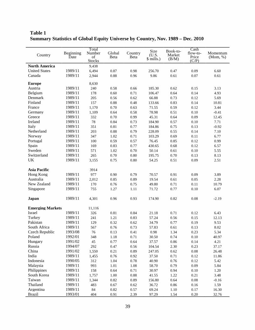
39

Table 1 Summary Statistics of Global Equity Universe by Country, Nov. 1989 – Dec. 2010

Country Beginning Date

Total Number

of Stocks

Global Beta

Country Beta

Size (U.S.

$ mills.)

Book-to-Market (B/M)

Cash flow-to-

Price (C/P)

Momentum (Mom, %)

North America

9,438 United States 1989/11 6,494 0.87 0.98 256.70 0.47 0.09 6.60

Canada 1989/11 2,944 0.88 0.96 9.86 0.61 0.07 0.61

Europe

8,630 Austria 1989/11 240 0.58 0.66 185.30 0.62 0.15 3.13

Belgium 1989/11 178 0.60 0.71 106.47 0.64 0.14 4.93 Denmark 1989/11 205 0.56 0.62 66.88 0.73 0.12 5.69 Finland 1989/11 157 0.88 0.48 133.66 0.83 0.14 10.81 France 1989/11 1,170 0.70 0.63 71.55 0.59 0.12 3.44 Germany 1989/11 1,109 0.64 0.58 78.98 0.51 0.10 -0.41 Greece 1989/11 332 0.70 0.99 45.31 0.64 0.09 12.45 Ireland 1989/11 78 0.84 0.73 184.90 0.57 0.10 7.71 Italy 1989/11 351 0.81 0.77 184.86 0.75 0.13 -0.92 Netherland 1989/11 203 0.88 0.79 228.09 0.55 0.14 7.10 Norway 1989/11 347 1.02 0.71 103.29 0.69 0.11 6.77 Portugal 1989/11 100 0.59 0.57 76.45 0.85 0.12 0.99 Spain 1989/11 169 0.83 0.77 430.65 0.68 0.12 6.57 Sweden 1989/11 571 1.02 0.70 50.14 0.61 0.10 5.55 Switzerland 1989/11 265 0.70 0.80 195.75 0.70 0.13 8.13 UK 1989/11 3,155 0.75 0.80 54.25 0.51 0.09 2.51

Asia Pacific

3914 Hong Kong 1989/11 977 0.90 0.79 70.57 0.91 0.09 3.89

Australia 1989/11 2,012 0.85 0.89 19.54 0.61 0.05 2.28 New Zealand 1989/11 170 0.76 0.75 49.80 0.71 0.11 10.79 Singapore 1989/11 755 1.27 1.11 71.72 0.77 0.10 6.07

Japan 1989/11 4,301 0.96 0.93 174.90 0.82 0.08 -2.19

Emerging Markets 11,116 Israel 1989/11 326 0.81 0.84 21.18 0.71 0.12 6.43

Turkey 1989/11 241 1.21 0.83 57.24 0.56 0.15 12.13 Pakistan 1989/11 129 0.32 0.62 34.79 0.77 0.19 9.53 South Africa 1989/11 567 0.76 0.73 57.83 0.61 0.13 8.02 Czech Republic 1993/08 76 0.13 0.41 0.98 1.34 0.23 5.34 Poland 1992/01 348 1.18 0.71 30.50 0.74 0.10 40.97 Hungary 1991/02 45 0.77 0.64 37.57 0.86 0.14 4.21 Russia 1994/07 292 0.47 0.56 104.54 2.30 0.23 37.17 China 1991/02 1,550 0.21 0.89 247.05 0.62 0.08 26.48 India 1989/11 1,455 0.76 0.92 37.50 0.71 0.12 11.86 Indonesia 1990/05 312 1.04 0.78 40.90 0.76 0.12 5.42 Malaysia 1989/11 993 1.01 1.08 58.70 0.79 0.09 5.84 Philippines 1989/11 158 0.64 0.71 30.97 0.94 0.10 1.20 South Korea 1989/11 1,757 1.00 0.88 41.55 1.22 0.21 3.48 Taiwan 1989/11 1,344 0.82 0.89 156.80 0.64 0.08 -0.16 Thailand 1989/11 483 0.67 0.62 36.72 0.86 0.16 1.59 Argentina 1989/11 84 0.82 0.57 69.24 1.10 0.17 16.30 Brazil 1993/01 404 0.91 2.39 97.29 1.54 0.20 32.76

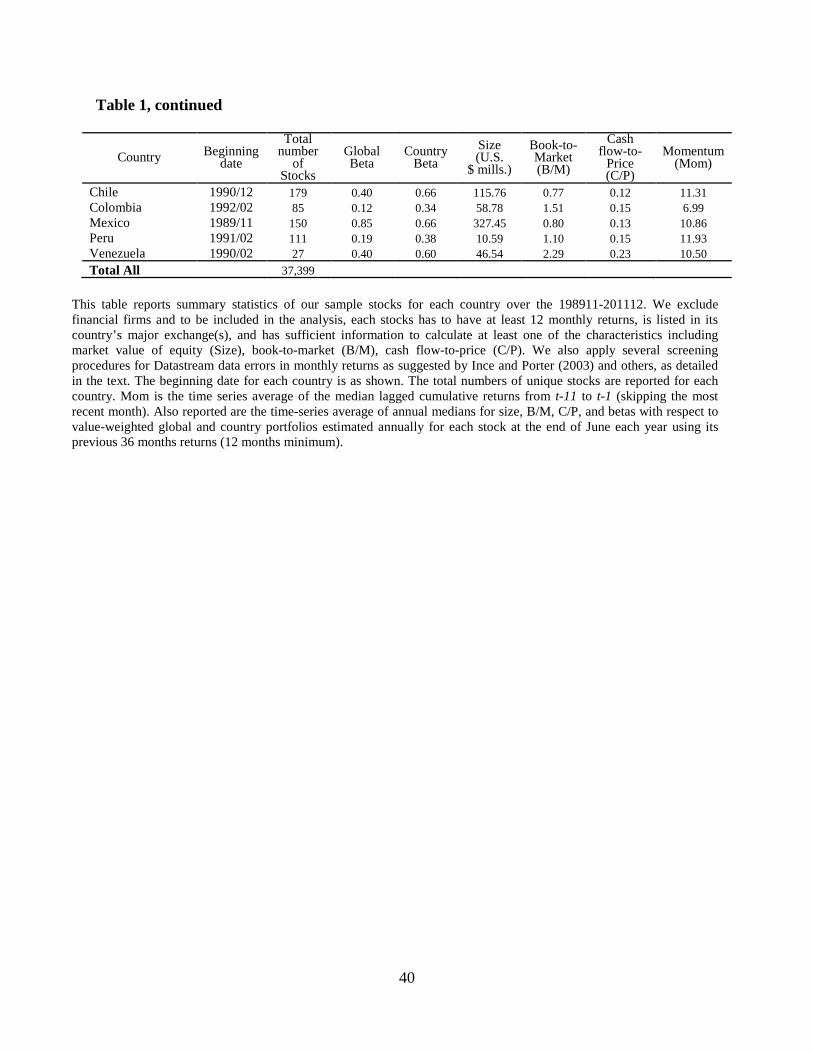
40

Table 1, continued

Country Beginning date

Total number

of Stocks

Global Beta

Country Beta

Size (U.S.

$ mills.)

Book-to-Market (B/M)

Cash flow-to-

Price (C/P)

Momentum (Mom)

Chile 1990/12 179 0.40 0.66 115.76 0.77 0.12 11.31 Colombia 1992/02 85 0.12 0.34 58.78 1.51 0.15 6.99 Mexico 1989/11 150 0.85 0.66 327.45 0.80 0.13 10.86 Peru 1991/02 111 0.19 0.38 10.59 1.10 0.15 11.93 Venezuela 1990/02 27 0.40 0.60 46.54 2.29 0.23 10.50 Total All

37,399

This table reports summary statistics of our sample stocks for each country over the 198911-201112. We exclude financial firms and to be included in the analysis, each stocks has to have at least 12 monthly returns, is listed in its country’s major exchange(s), and has sufficient information to calculate at least one of the characteristics including market value of equity (Size), book-to-market (B/M), cash flow-to-price (C/P). We also apply several screening procedures for Datastream data errors in monthly returns as suggested by Ince and Porter (2003) and others, as detailed in the text. The beginning date for each country is as shown. The total numbers of unique stocks are reported for each country. Mom is the time series average of the median lagged cumulative returns from t-11 to t-1 (skipping the most recent month). Also reported are the time-series average of annual medians for size, B/M, C/P, and betas with respect to value-weighted global and country portfolios estimated annually for each stock at the end of June each year using its previous 36 months returns (12 months minimum).

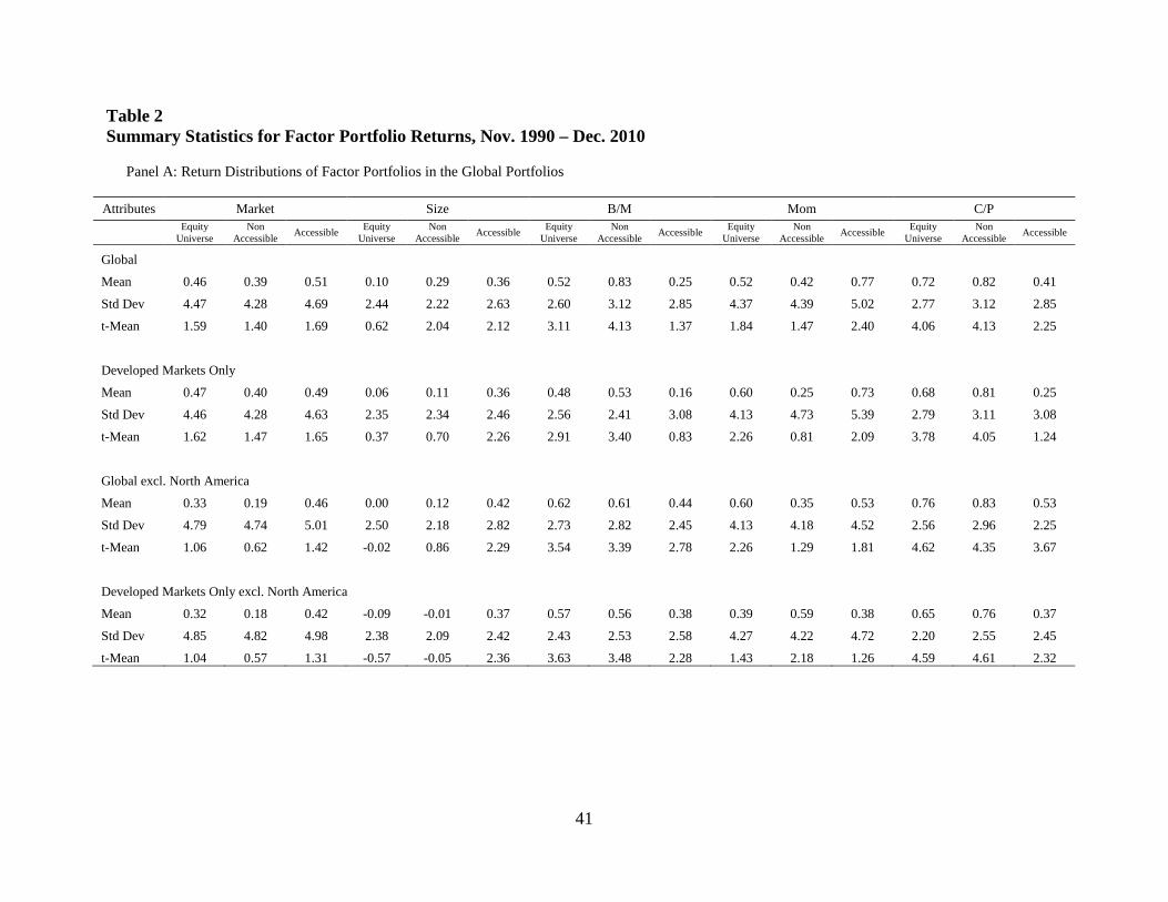
41

Table 2 Summary Statistics for Factor Portfolio Returns, Nov. 1990 – Dec. 2010

Panel A: Return Distributions of Factor Portfolios in the Global Portfolios

Attributes Market Size B/M Mom C/P

Equity Universe

Non Accessible Accessible Equity

Universe Non

Accessible Accessible Equity Universe

Non Accessible Accessible Equity

Universe Non

Accessible Accessible Equity Universe

Non Accessible Accessible

Global Mean 0.46 0.39 0.51 0.10 0.29 0.36 0.52 0.83 0.25 0.52 0.42 0.77 0.72 0.82 0.41

Std Dev 4.47 4.28 4.69 2.44 2.22 2.63 2.60 3.12 2.85 4.37 4.39 5.02 2.77 3.12 2.85

t-Mean 1.59 1.40 1.69 0.62 2.04 2.12 3.11 4.13 1.37 1.84 1.47 2.40 4.06 4.13 2.25

Developed Markets Only

Mean 0.47 0.40 0.49 0.06 0.11 0.36 0.48 0.53 0.16 0.60 0.25 0.73 0.68 0.81 0.25

Std Dev 4.46 4.28 4.63 2.35 2.34 2.46 2.56 2.41 3.08 4.13 4.73 5.39 2.79 3.11 3.08

t-Mean 1.62 1.47 1.65 0.37 0.70 2.26 2.91 3.40 0.83 2.26 0.81 2.09 3.78 4.05 1.24

Global excl. North America

Mean 0.33 0.19 0.46 0.00 0.12 0.42 0.62 0.61 0.44 0.60 0.35 0.53 0.76 0.83 0.53

Std Dev 4.79 4.74 5.01 2.50 2.18 2.82 2.73 2.82 2.45 4.13 4.18 4.52 2.56 2.96 2.25

t-Mean 1.06 0.62 1.42 -0.02 0.86 2.29 3.54 3.39 2.78 2.26 1.29 1.81 4.62 4.35 3.67

Developed Markets Only excl. North America

Mean 0.32 0.18 0.42 -0.09 -0.01 0.37 0.57 0.56 0.38 0.39 0.59 0.38 0.65 0.76 0.37

Std Dev 4.85 4.82 4.98 2.38 2.09 2.42 2.43 2.53 2.58 4.27 4.22 4.72 2.20 2.55 2.45

t-Mean 1.04 0.57 1.31 -0.57 -0.05 2.36 3.63 3.48 2.28 1.43 2.18 1.26 4.59 4.61 2.32

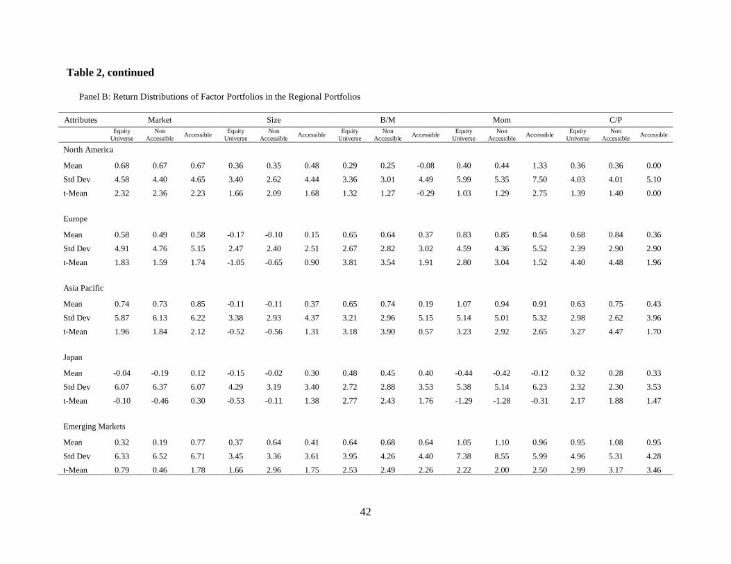
42

Table 2, continued

Panel B: Return Distributions of Factor Portfolios in the Regional Portfolios

Attributes Market Size B/M Mom C/P

Equity Universe

Non Accessible Accessible Equity

Universe Non

Accessible Accessible Equity Universe

Non Accessible Accessible Equity

Universe Non

Accessible Accessible Equity Universe

Non Accessible Accessible

North America

Mean 0.68 0.67 0.67 0.36 0.35 0.48 0.29 0.25 -0.08 0.40 0.44 1.33 0.36 0.36 0.00

Std Dev 4.58 4.40 4.65 3.40 2.62 4.44 3.36 3.01 4.49 5.99 5.35 7.50 4.03 4.01 5.10

t-Mean 2.32 2.36 2.23 1.66 2.09 1.68 1.32 1.27 -0.29 1.03 1.29 2.75 1.39 1.40 0.00

Europe

Mean 0.58 0.49 0.58 -0.17 -0.10 0.15 0.65 0.64 0.37 0.83 0.85 0.54 0.68 0.84 0.36

Std Dev 4.91 4.76 5.15 2.47 2.40 2.51 2.67 2.82 3.02 4.59 4.36 5.52 2.39 2.90 2.90

t-Mean 1.83 1.59 1.74 -1.05 -0.65 0.90 3.81 3.54 1.91 2.80 3.04 1.52 4.40 4.48 1.96

Asia Pacific

Mean 0.74 0.73 0.85 -0.11 -0.11 0.37 0.65 0.74 0.19 1.07 0.94 0.91 0.63 0.75 0.43

Std Dev 5.87 6.13 6.22 3.38 2.93 4.37 3.21 2.96 5.15 5.14 5.01 5.32 2.98 2.62 3.96

t-Mean 1.96 1.84 2.12 -0.52 -0.56 1.31 3.18 3.90 0.57 3.23 2.92 2.65 3.27 4.47 1.70

Japan

Mean -0.04 -0.19 0.12 -0.15 -0.02 0.30 0.48 0.45 0.40 -0.44 -0.42 -0.12 0.32 0.28 0.33

Std Dev 6.07 6.37 6.07 4.29 3.19 3.40 2.72 2.88 3.53 5.38 5.14 6.23 2.32 2.30 3.53

t-Mean -0.10 -0.46 0.30 -0.53 -0.11 1.38 2.77 2.43 1.76 -1.29 -1.28 -0.31 2.17 1.88 1.47

Emerging Markets

Mean 0.32 0.19 0.77 0.37 0.64 0.41 0.64 0.68 0.64 1.05 1.10 0.96 0.95 1.08 0.95

Std Dev 6.33 6.52 6.71 3.45 3.36 3.61 3.95 4.26 4.40 7.38 8.55 5.99 4.96 5.31 4.28

t-Mean 0.79 0.46 1.78 1.66 2.96 1.75 2.53 2.49 2.26 2.22 2.00 2.50 2.99 3.17 3.46

43

Table 2, continued

This table shows the summary statistics for explanatory returns. It includes five regional portfolios for North America, Europe, Japan, Asia Pacific (excluding Japan) and Emerging Markets. Four sets of global portfolios are also reported, including Global portfolios that combine all the five regions, Developed Markets portfolios that combine the first four regions, Global portfolios excluding North America, Developed Markets portfolios excluding North America. For each scenario, it shows the explanatory returns for three samples, the whole sample (“Equity Universe” in the table), the subset of non cross-listed stocks (“Non Accessible” in the table), the subset of cross-listed stocks, the Main CL Sample, which stands for the globally accessible sample (“Accessible” in the table). We form portfolios at the end of June of each year t by sorting stocks in a region into two market cap and three book-to-market (B/M) or cash flow-to-price (C/P) groups. Big stocks are those in the top 90% of market cap for the region, and small stocks are those in the bottom 10% (Fama and French, 2011). The B/M or C/P breakpoints for the five regions are the 30th and 70th percentiles of B/M for the big stocks from the globally accessible sample for each given region. The global portfolios use global size breaks, but we use the B/M or C/P breakpoints for the five regions to allocate the stocks of these regions to the global portfolios. The independent 2×3 sorts on size and B/M (or C/P) produce six value-weighted portfolios, SG, SN, SV, BG, BN and BV, where S and B indicate small or big and G, N, and V indicate growth, neutral and value. The factor mimicking portfolios (FMPs) based on size is the equally-weighted average of the returns on the three small stock portfolios for the region minus the equally-weighted average of the returns on the three big stock portfolios where all the six portfolios are all based on B/M. The FMPs based on B/M (or C/P) are calculated as the equally-weighted average of value-growth returns for small and big stocks, SV-SG and BV-BG. The 2×3 sorts on size and lagged momentum are similar, but the size/momentum portfolios are formed monthly. For portfolios formed at the end of month t, the lagged momentum return is a stock’s cumulative return for t-11 to t-1. The independent 2×3 sorts on size and momentum produce six value-weighted portfolios, SL, SN, SW, BL, BN and BW, where S and B indicate small and big, and L, N, and W indicate losers, neutral, and winners. The FMPs based on momentum is constructed as the equally-weighted average of WMLS=SW-SL and WMLB=BW-BL. B/M(C/P) breakpoints are the same for all three samples within each scenario, the globally accessible sample uses its own size and momentum breakpoints, and the purely local sample uses regional size and momentum breakpoints. All returns are in U.S. dollars. Market is the return on a value-weighted market portfolio globally or for the region minus the U.S. one month Treasury bill yield. Mean and Std Dev are the mean and standard deviation of the return, and t-Mean is the ratio of Mean to its standard error.

44

Table 3 Summary Statistics for the 25 size/B/M Excess Returns, Nov. 1990 – Dec. 2010

Mean Standard Deviation Low 2 3 4 High Low 2 3 4 High

Global Small 0.06 0.55 1.36 0.93 1.25

6.55 5.95 8.42 5.06 4.91

2 0.09 0.59 0.64 0.76 0.94

6.02 5.51 5.03 4.89 4.97 3 0.15 0.37 0.56 0.62 0.83

5.75 5.37 5.18 4.84 5.06

4 0.40 0.47 0.59 0.60 0.81

6.05 5.02 5.00 4.74 5.08 Big 0.28 0.49 0.46 0.62 0.54

4.87 4.44 4.43 4.38 4.73

Developed Markets Only Small 0.05 0.58 0.88 0.84 1.10

6.66 5.72 5.88 5.08 4.65

2 0.11 0.42 0.58 0.70 0.80

6.50 5.61 5.02 4.70 4.87 3 0.14 0.37 0.46 0.58 0.75

6.16 5.50 5.32 4.74 5.00

4 0.42 0.36 0.59 0.59 0.74

6.29 4.97 4.81 4.80 5.09 Big 0.26 0.49 0.42 0.63 0.51

4.86 4.38 4.44 4.28 4.74

Global excl. North America (NA) Small -0.15 0.30 0.66 0.66 1.00

6.77 5.71 5.32 5.00 5.16

2 -0.11 0.36 0.88 0.63 0.74

6.03 5.58 8.01 5.08 5.26 3 -0.05 0.25 0.34 0.51 0.75

5.73 5.57 5.25 5.19 5.40

4 0.12 0.32 0.40 0.47 0.70

5.70 5.34 5.27 5.22 5.60 Big 0.02 0.30 0.43 0.54 0.65

5.32 4.98 4.89 4.91 5.27

Developed Markets Only excl. North America (NA) Small -0.15 0.23 0.43 0.54 0.76

6.84 5.46 5.25 4.86 4.87

2 -0.31 0.19 0.31 0.47 0.47

6.18 6.08 5.03 4.90 5.08 3 -0.12 0.12 0.28 0.50 0.53

6.04 5.49 5.35 5.11 5.41

4 0.02 0.20 0.33 0.37 0.60

6.10 5.21 5.21 5.27 5.58 Big -0.04 0.29 0.37 0.55 0.64

5.30 4.96 4.96 4.87 5.39

North America Small 0.89 1.14 1.45 1.32 1.64

8.90 7.34 7.68 6.56 6.00

2 0.61 0.94 1.03 1.00 1.20

8.37 7.22 6.51 5.48 5.75 3 0.96 0.67 0.85 0.92 1.11

8.42 6.51 5.75 4.93 5.31

4 0.89 0.75 0.93 0.77 0.99

7.71 5.75 5.29 5.06 5.20 Big 0.54 0.67 0.53 0.79 0.55 5.21 4.61 4.42 4.23 4.72

Europe Small -0.20 0.07 0.51 0.50 0.87

6.59 5.62 5.40 5.16 5.14

2 0.14 0.28 0.40 0.72 0.96

6.47 5.62 5.55 5.32 5.66 3 0.19 0.38 0.41 0.72 0.90

6.46 5.71 5.37 5.51 5.92

4 0.35 0.39 0.66 0.68 0.75

6.06 5.19 5.28 5.47 5.81 Big 0.26 0.52 0.58 0.84 0.86

5.34 4.79 5.29 5.17 5.63

Asia Pacific Small 0.68 0.93 1.30 1.45 2.11

11.34 9.80 8.78 8.11 8.78

2 0.17 0.93 0.60 1.03 1.12

8.23 8.21 8.06 7.41 7.93 3 -0.15 0.32 0.77 1.03 0.94

7.97 6.84 7.25 7.11 7.32

4 0.99 1.08 0.79 0.94 0.92

7.14 8.28 6.41 6.13 7.38 Big 0.54 1.02 0.56 0.77 1.24

6.39 6.31 6.54 5.77 7.94

45

Table 3, continued

Mean Standard Deviation Low 2 3 4 High Low 2 3 4 High

Japan Small -0.46 -0.05 -0.06 0.18 0.09

10.07 7.89 7.57 7.20 6.98

2 -0.55 -0.13 -0.15 -0.05 -0.02

8.90 8.19 7.50 7.10 6.97 3 -0.47 -0.21 -0.14 -0.08 0.03

8.39 8.19 7.19 7.03 7.05

4 -0.51 -0.12 -0.09 -0.03 0.19

7.82 7.11 6.68 6.63 6.77 Big -0.48 -0.06 0.12 0.21 0.39

6.90 6.32 5.78 5.66 6.33

Emerging Markets Small 0.13 0.55 1.45 1.04 1.72

10.09 7.66 8.50 7.27 7.55

2 0.36 0.92 0.73 1.02 1.31

7.77 7.42 7.30 6.82 7.55 3 0.26 0.86 0.56 1.00 1.41

7.32 7.33 7.43 6.92 7.14

4 0.19 0.46 0.56 0.74 1.22

6.78 6.77 6.61 6.50 7.39 Big 0.37 0.40 0.63 0.57 0.91

6.42 6.72 6.32 6.89 7.17

This table shows the summary statistics for the 25 size/B/M excess returns. As in Fama and French (2011), at the end of June of each year we construct 25 size/B/M portfolios for each region. The size breakpoints are the 3rd, 7th, 13th, and 25th percentiles of aggregate market cap for a region. The B/M quintile breakpoints use the big stocks (top 90% of market cap) of a region. Regional quintile B/M breakpoints are used to allocate the stocks of these regions to the global test asset portfolios. The intersections of the 5×5 independent size and B/M sorts for a region produce 25 value-weighted size/B/M portfolios.

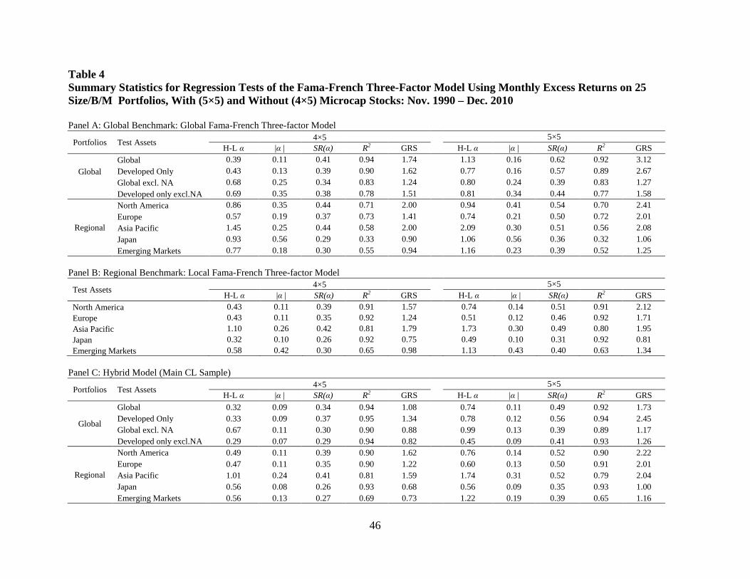
46

Table 4 Summary Statistics for Regression Tests of the Fama-French Three-Factor Model Using Monthly Excess Returns on 25 Size/B/M Portfolios, With (5×5) and Without (4×5) Microcap Stocks: Nov. 1990 – Dec. 2010 Panel A: Global Benchmark: Global Fama-French Three-factor Model

Portfolios Test Assets 4×5 5×5 H-L α |α | SR(α) R2 GRS H-L α |α | SR(α) R2 GRS

Global

Global 0.39 0.11 0.41 0.94 1.74 1.13 0.16 0.62 0.92 3.12 Developed Only 0.43 0.13 0.39 0.90 1.62 0.77 0.16 0.57 0.89 2.67 Global excl. NA 0.68 0.25 0.34 0.83 1.24 0.80 0.24 0.39 0.83 1.27 Developed only excl.NA 0.69 0.35 0.38 0.78 1.51 0.81 0.34 0.44 0.77 1.58

Regional

North America 0.86 0.35 0.44 0.71 2.00 0.94 0.41 0.54 0.70 2.41 Europe 0.57 0.19 0.37 0.73 1.41 0.74 0.21 0.50 0.72 2.01 Asia Pacific 1.45 0.25 0.44 0.58 2.00 2.09 0.30 0.51 0.56 2.08 Japan 0.93 0.56 0.29 0.33 0.90 1.06 0.56 0.36 0.32 1.06 Emerging Markets 0.77 0.18 0.30 0.55 0.94 1.16 0.23 0.39 0.52 1.25

Panel B: Regional Benchmark: Local Fama-French Three-factor Model

Test Assets 4×5 5×5 H-L α |α | SR(α) R2 GRS H-L α |α | SR(α) R2 GRS

North America 0.43 0.11 0.39 0.91 1.57 0.74 0.14 0.51 0.91 2.12 Europe 0.43 0.11 0.35 0.92 1.24 0.51 0.12 0.46 0.92 1.71 Asia Pacific 1.10 0.26 0.42 0.81 1.79 1.73 0.30 0.49 0.80 1.95 Japan 0.32 0.10 0.26 0.92 0.75 0.49 0.10 0.31 0.92 0.81 Emerging Markets 0.58 0.42 0.30 0.65 0.98 1.13 0.43 0.40 0.63 1.34

Panel C: Hybrid Model (Main CL Sample)

Portfolios Test Assets 4×5 5×5 H-L α |α | SR(α) R2 GRS H-L α |α | SR(α) R2 GRS

Global

Global 0.32 0.09 0.34 0.94 1.08 0.74 0.11 0.49 0.92 1.73 Developed Only 0.33 0.09 0.37 0.95 1.34 0.78 0.12 0.56 0.94 2.45 Global excl. NA 0.67 0.11 0.30 0.90 0.88 0.99 0.13 0.39 0.89 1.17 Developed only excl.NA 0.29 0.07 0.29 0.94 0.82 0.45 0.09 0.41 0.93 1.26

Regional

North America 0.49 0.11 0.39 0.90 1.62 0.76 0.14 0.52 0.90 2.22 Europe 0.47 0.11 0.35 0.90 1.22 0.60 0.13 0.50 0.91 2.01 Asia Pacific 1.01 0.24 0.41 0.81 1.59 1.74 0.31 0.52 0.79 2.04 Japan 0.56 0.08 0.26 0.93 0.68 0.56 0.09 0.35 0.93 1.00 Emerging Markets 0.56 0.13 0.27 0.69 0.73 1.22 0.19 0.39 0.65 1.16

47

Table 4, continued The regressions use the global, local and hybrid version of the Fama-French three-factor model to explain the returns on four sets of global portfolios and five sets of regional portfolios on North America, Europe, Japan, Asia Pacific(excluding Japan), and Emerging Markets formed on size and B/M. The 5×5 results include five size quintiles, the 4×5 results exclude microcap portfolios. The GRS statistic tests whether all intercepts in a set of 25 (5×5) or 20 (4×5) regressions are zero; H-L α is the difference between the highest and lowest intercepts for a set of regressions; |α| is the average absolute intercepts; R2 is the average adjusted R2; SR(α) is the Sharpe ratio for the intercepts. With 25 portfolios and 242 monthly returns, critical values of the GRS statistic for all models are: 90%: 1.41; 95%: 1.56; 97.5%: 1.69; 99%: 1.86 and 99.9%: 2.26. With 20 portfolios and 242 monthly returns, critical values of the GRS statistic for all models are: 90%: 1.45; 95%: 1.62; 97.5%: 1.78; 99%: 1.95 and 99.9%: 2.41. Three classes of models are investigated:

Global Fama-French Three-factor Model: 𝑅𝑖 − 𝑅𝑓 = 𝛼𝑖𝐺 + 𝛽𝑖𝐺�𝑅𝑚𝐺 − 𝑅𝑓� + 𝑠𝑖𝐺𝐹𝑆𝑖𝑧𝑒𝐺 + ℎ𝑖𝐺𝐹𝐵/𝑀𝐺 + 𝜀𝑖

Local Fama-French Three-factor Model: 𝑅𝑖 − 𝑅𝑓 = 𝛼𝑖𝐿 + 𝛽𝑖𝐿�𝑅𝑚𝐿 − 𝑅𝑓� + 𝑠𝑖𝐿𝐹𝑆𝑖𝑧𝑒𝐿 + ℎ𝑖𝐿𝐹𝐵/𝑀𝐿 + 𝜀𝑖

Hybrid Fama-French Three-factor Model: 𝑅𝑖 − 𝑅𝑓 = 𝛼𝑖𝐻 + 𝛽𝑖𝐶𝐿�𝑅𝑚𝐶𝐿 − 𝑅𝑓� + 𝛽𝑖𝑁𝐶𝐿�𝑅𝑚𝑁𝐶𝐿 − 𝑅𝑓� + 𝑠𝑖𝐶𝐿𝐹𝑆𝑖𝑧𝑒𝐶𝐿 + 𝑠𝑖𝑁𝐶𝐿𝐹𝑆𝑖𝑧𝑒𝑁𝐶𝐿 + ℎ𝑖𝐶𝐿𝐹𝐵/𝑀

𝐶𝐿 + ℎ𝑖𝑁𝐶𝐿𝐹𝐵/𝑀𝑁𝐶𝐿 + 𝜀𝑖

The superscript “G” on the market and factor portfolios implies that they are constructed from all stocks around the world and the superscript designation of “L” on the market and factor portfolios implies that they are constructed only from local - or regional, in our experiments - stocks. The superscript “H” denotes the intercept for the hybrid model. The superscript “CL” denotes a market or factor portfolio comprised of stocks only in the globally-accessible sample, which is represented by the sample of secondary cross-listings (CL) in this study, and the superscript “NCL” denotes a market or factor portfolio comprised of the purely-local stocks from the specific region (those not secondarily cross-listed overseas) for which the test is performed. The Main CL Sample is used here.

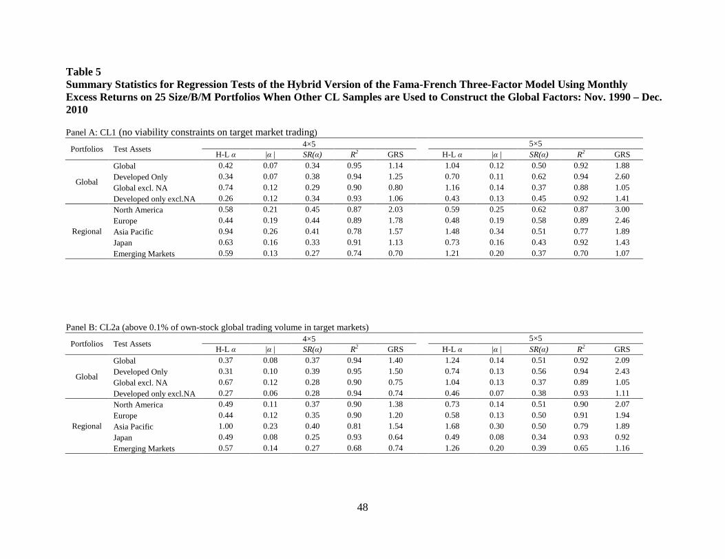
48

Table 5 Summary Statistics for Regression Tests of the Hybrid Version of the Fama-French Three-Factor Model Using Monthly Excess Returns on 25 Size/B/M Portfolios When Other CL Samples are Used to Construct the Global Factors: Nov. 1990 – Dec. 2010 Panel A: CL1 (no viability constraints on target market trading)

Portfolios Test Assets 4×5 5×5 H-L α |α | SR(α) R2 GRS H-L α |α | SR(α) R2 GRS

Global

Global 0.42 0.07 0.34 0.95 1.14 1.04 0.12 0.50 0.92 1.88 Developed Only 0.34 0.07 0.38 0.94 1.25 0.70 0.11 0.62 0.94 2.60 Global excl. NA 0.74 0.12 0.29 0.90 0.80 1.16 0.14 0.37 0.88 1.05 Developed only excl.NA 0.26 0.12 0.34 0.93 1.06 0.43 0.13 0.45 0.92 1.41

Regional

North America 0.58 0.21 0.45 0.87 2.03 0.59 0.25 0.62 0.87 3.00 Europe 0.44 0.19 0.44 0.89 1.78 0.48 0.19 0.58 0.89 2.46 Asia Pacific 0.94 0.26 0.41 0.78 1.57 1.48 0.34 0.51 0.77 1.89 Japan 0.63 0.16 0.33 0.91 1.13 0.73 0.16 0.43 0.92 1.43 Emerging Markets 0.59 0.13 0.27 0.74 0.70 1.21 0.20 0.37 0.70 1.07

Panel B: CL2a (above 0.1% of own-stock global trading volume in target markets)

Portfolios Test Assets 4×5 5×5 H-L α |α | SR(α) R2 GRS H-L α |α | SR(α) R2 GRS

Global

Global 0.37 0.08 0.37 0.94 1.40 1.24 0.14 0.51 0.92 2.09 Developed Only 0.31 0.10 0.39 0.95 1.50 0.74 0.13 0.56 0.94 2.43 Global excl. NA 0.67 0.12 0.28 0.90 0.75 1.04 0.13 0.37 0.89 1.05 Developed only excl.NA 0.27 0.06 0.28 0.94 0.74 0.46 0.07 0.38 0.93 1.11

Regional

North America 0.49 0.11 0.37 0.90 1.38 0.73 0.14 0.51 0.90 2.07 Europe 0.44 0.12 0.35 0.90 1.20 0.58 0.13 0.50 0.91 1.94 Asia Pacific 1.00 0.23 0.40 0.81 1.54 1.68 0.30 0.50 0.79 1.89 Japan 0.49 0.08 0.25 0.93 0.64 0.49 0.08 0.34 0.93 0.92 Emerging Markets 0.57 0.14 0.27 0.68 0.74 1.26 0.20 0.39 0.65 1.16

49

Table 5, continued Panel C: CL2b (non-zero target market trading in trailing 12 months)

Portfolios Test Assets 4×5 5×5 H-L α |α | SR(α) R2 GRS H-L α |α | SR(α) R2 GRS

Global

Global 0.39 0.09 0.38 0.93 1.54 1.05 0.14 0.53 0.91 2.28 Developed Only 0.33 0.11 0.40 0.92 1.61 0.68 0.14 0.58 0.91 2.72 Global excl. NA 0.67 0.10 0.34 0.90 1.23 0.89 0.12 0.43 0.89 1.48 Developed only excl.NA 0.45 0.10 0.35 0.92 1.24 0.67 0.11 0.44 0.92 1.58

Regional

North America 0.41 0.11 0.37 0.81 1.39 0.84 0.16 0.51 0.82 2.11 Europe 0.46 0.09 0.35 0.90 1.25 0.59 0.11 0.48 0.90 1.89 Asia Pacific 1.08 0.24 0.41 0.80 1.66 1.76 0.31 0.51 0.79 2.04 Japan 0.59 0.19 0.33 0.91 1.13 0.61 0.17 0.37 0.91 1.10 Emerging Markets 0.53 0.14 0.25 0.68 0.62 1.29 0.21 0.38 0.65 1.15

Panel D: CL2c (impose top 50% of market cap from target markets to the Main CL Sample)

Portfolios Test Assets 4×5 5×5 H-L α |α | SR(α) R2 GRS H-L α |α | SR(α) R2 GRS

Global

Global 0.32 0.08 0.33 0.94 0.98 0.67 0.11 0.46 0.92 1.50 Developed Only 0.48 0.06 0.36 0.95 1.22 0.55 0.10 0.53 0.94 2.04 Global excl. NA 0.62 0.12 0.29 0.90 0.83 0.95 0.13 0.38 0.89 1.10 Developed only excl.NA 0.22 0.06 0.27 0.94 0.69 0.40 0.07 0.38 0.93 1.06

Regional

North America 0.60 0.14 0.52 0.90 2.75 0.60 0.16 0.62 0.90 3.08 Europe 0.45 0.11 0.35 0.90 1.24 0.53 0.13 0.49 0.91 1.86 Asia Pacific 0.94 0.23 0.39 0.80 1.51 1.71 0.30 0.51 0.79 1.99 Japan 0.56 0.08 0.26 0.92 0.69 0.56 0.09 0.36 0.93 1.01 Emerging Markets 0.59 0.13 0.26 0.68 0.68 1.24 0.20 0.38 0.64 1.13

50

Table 5, continued The regressions use the hybrid model to explain the returns on four sets of global portfolios and five sets of regional portfolios on North America, Europe, Japan, Asia Pacific(excluding Japan), and Emerging Markets formed on size and B/M. The global factor portfolios are based on other globally accessible samples, where CL1 refers to the sample without viability constraints, CL2a is the sample with relative viability constraint I, CL2b is the sample with absolute viable constraint and CL2c is the sample where the stocks in the top 50% of market cap from each target market are added into the Main CL Sample. The selection criteria are described in the Appendix. The 5×5 results include five size quintiles, the 4×5 results exclude microcap portfolios. The GRS statistic tests whether all intercepts in a set of 25 (5×5) or 20 (4×5) regressions are zero; H-L α is the difference between the highest and lowest intercepts for a set of regressions; |α| is the average absolute intercept; R2 is the average adjusted R2; SR(α) is the Sharpe ratio for the intercepts. With 25 portfolios and 242 monthly returns, critical values of the GRS statistic for all models are: 90%: 1.41; 95%: 1.56; 97.5%: 1.69; 99%: 1.86 and 99.9%: 2.26. With 20 portfolios and 242 monthly returns, critical values of the GRS statistic for all models are: 90%: 1.45; 95%: 1.62; 97.5%: 1.78; 99%: 1.95 and 99.9%: 2.41. The hybrid model based on the Fama-French three-factor model is:

Rit – Rft = αHi + βCL

i (RCLmt – Rft) + sCL

i FCLSize,t + hCL

i FCLB/M,t + βNCL

i (RNCLmt – Rft) + sNCL

i FNCLSize,t + hNCL

i FNCLB/M,t + εi,t

The superscript “H” denotes the intercept for the hybrid model, the superscript “CL” denotes a market or factor portfolio comprised of stocks only in the globally-accessible sample, which is represented by the sample of secondary cross-listings (CL) in this study, and the superscript “NCL” denotes a market or factor portfolio comprised of the purely-local stocks from the specific region (those not secondarily cross-listed overseas) for which the test is performed.

51

Table 6 Summary Statistics for Regression Tests of the Carhart Four-Factor Model Using Monthly Excess Returns on 25 Size/Momentum Portfolios, With (5×5) and Without (4×5) Microcap Stocks: Nov. 1990 – Dec. 2010 Panel A: Global Benchmark: Global Carhart Four-factor Model

Portfolios Test Assets 4×5 5×5 H-L α |α | SR(α) R2 GRS H-L α |α | SR(α) R2 GRS

Global

Global 0.57 0.12 0.43 0.92 1.89 1.18 0.20 0.53 0.89 2.20 Developed Only 0.71 0.14 0.45 0.89 2.05 0.97 0.16 0.59 0.88 2.72 Global excl. NA 0.89 0.25 0.44 0.81 1.96 1.05 0.26 0.49 0.80 1.88 Developed only excl.NA 0.71 0.32 0.37 0.77 1.42 0.95 0.31 0.44 0.75 1.56

Regional

North America 0.82 0.45 0.37 0.72 1.37 1.22 0.51 0.51 0.72 2.02 Europe 1.22 0.23 0.51 0.73 2.68 1.75 0.29 0.67 0.71 3.57 Asia Pacific 1.61 0.34 0.52 0.58 2.74 2.00 0.36 0.64 0.58 3.21 Japan 1.57 0.49 0.43 0.34 1.84 1.57 0.50 0.52 0.33 2.11 Emerging Markets 2.53 0.47 0.44 0.45 1.96 2.53 0.56 0.52 0.46 2.15

Panel B: Regional Benchmark: Local Carhart Four -factor Model

Test Assets 4×5 5×5 H-L α |α | SR(α) R2 GRS H-L α |α | SR(α) R2 GRS

North America 0.54 0.10 0.30 0.91 0.94 1.05 0.15 0.45 0.91 1.64 Europe 0.98 0.20 0.55 0.91 2.98 1.26 0.23 0.68 0.91 3.56 Asia Pacific 0.84 0.23 0.47 0.83 2.17 1.26 0.28 0.64 0.83 3.12 Japan 0.63 0.19 0.36 0.92 1.37 0.78 0.20 0.47 0.92 1.79 Emerging Markets 0.84 0.60 0.43 0.62 1.90 1.07 0.69 0.51 0.62 2.13

Panel C: Hybrid Model (Main CL Sample)

Portfolios Test Assets 4×5 5×5 H-L α |α | SR(α) R2 GRS H-L α |α | SR(α) R2 GRS

Global

Global 0.42 0.13 0.44 0.93 1.73 0.74 0.15 0.52 0.90 1.91 Developed Only 0.64 0.13 0.41 0.94 1.60 0.91 0.15 0.54 0.93 2.17 Global excl. NA 0.90 0.16 0.47 0.88 2.04 0.90 0.20 0.50 0.87 1.82 Developed only excl.NA 0.89 0.13 0.43 0.93 1.70 0.98 0.15 0.52 0.92 1.97

Regional

North America 0.75 0.15 0.35 0.90 1.22 0.99 0.20 0.47 0.89 1.75 Europe 0.94 0.20 0.55 0.90 2.90 1.23 0.23 0.69 0.90 3.60 Asia Pacific 0.83 0.25 0.49 0.83 2.25 1.37 0.32 0.66 0.83 3.12 Japan 0.77 0.14 0.40 0.93 1.50 0.77 0.14 0.52 0.92 2.01 Emerging Markets 1.30 0.38 0.41 0.64 1.58 1.40 0.44 0.49 0.65 1.78

52

Table 6, continued

The regressions use the global, local and hybrid version of the Carhart four-factor model to explain the returns on four sets of global portfolios and five sets of regional portfolios on North America, Europe, Japan, Asia Pacific(excluding Japan), and Emerging Markets formed on size and momentum. The 5×5 results include five size quintiles, the 4×5 results exclude microcap portfolios. The GRS statistic tests whether all intercepts in a set of 25 (5×5) or 20 (4×5) regressions are zero; H-L α is the difference between the highest and lowest intercepts for a set of regressions; |α| is the average absolute intercept; R2 is the average adjusted R2; SR(α) is the Sharpe ratio for the intercepts. With 25 portfolios and 242 monthly returns, critical values of the GRS statistic for all models are: 90%: 1.41; 95%: 1.56; 97.5%: 1.69; 99%: 1.86 and 99.9%: 2.26. With 20 portfolios and 242 monthly returns, critical values of the GRS statistic for all models are: 90%: 1.45; 95%: 1.62; 97.5%: 1.78; 99%: 1.95 and 99.9%: 2.41. Three classes of models are investigated:

Global Carhart Four-factor Model: 𝑅𝑖 − 𝑅𝑓 = 𝛼𝑖𝐺 + 𝛽𝑖𝐺�𝑅𝑚𝐺 − 𝑅𝑓� + 𝑠𝑖𝐺𝐹𝑆𝑖𝑧𝑒𝐺 + ℎ𝑖𝐺𝐹𝐵/𝑀𝐺 + 𝑚𝑖

𝐺𝐹𝑀𝑜𝑚𝐺 + 𝜀𝑖 Local Carhart Four-factor Model: 𝑅𝑖 − 𝑅𝑓 = 𝛼𝑖𝐿 + 𝛽𝑖𝐿�𝑅𝑚𝐿 − 𝑅𝑓� + 𝑠𝑖𝐿𝐹𝑆𝑖𝑧𝑒𝐿 + ℎ𝑖𝐿𝐹𝐵/𝑀

𝐿 + 𝑚𝑖𝐿𝐹𝑀𝑜𝑚𝐿 + 𝜀𝑖

Hybrid Carhart Four-factor Model: 𝑅𝑖 − 𝑅𝑓 = 𝛼𝑖𝐻 + 𝛽𝑖𝐶𝐿�𝑅𝑚𝐶𝐿 − 𝑅𝑓� + 𝛽𝑖𝑁𝐶𝐿�𝑅𝑚𝑁𝐶𝐿 − 𝑅𝑓� + 𝑠𝑖𝐶𝐿𝐹𝑆𝑖𝑧𝑒𝐶𝐿 + 𝑠𝑖𝑁𝐶𝐿𝐹𝑆𝑖𝑧𝑒𝑁𝐶𝐿 + ℎ𝑖𝐶𝐿𝐹𝐵/𝑀𝐶𝐿 + ℎ𝑖𝑁𝐶𝐿𝐹𝐵/𝑀

𝑁𝐶𝐿 + 𝑚𝑖𝐶𝐿𝐹𝑀𝑜𝑚𝐶𝐿 + 𝑚𝑖

𝑁𝐶𝐿𝐹𝑀𝑜𝑚𝑁𝐶𝐿 + 𝜀𝑖 The superscript “G” on the market and factor portfolios implies that they are constructed from all stocks around the world and the superscript designation of “L” on the market and factor portfolios implies that they are constructed only from local - or regional, in our experiments - stocks. The superscript “H” denotes the intercept for the hybrid model. The superscript “CL” denotes a market or factor portfolio comprised of stocks only in the globally-accessible sample, which is represented by the sample of secondary cross-listings (CL) in this study, and the superscript “NCL” denotes a market or factor portfolio comprised of the purely-local stocks from the specific region (those not secondarily cross-listed overseas) for which the test is performed. The Main CL Sample is used here.

53

Table 7 Summary Statistics for Regression Tests of the Carhart Four-Factor Model Using Monthly Excess Returns on 25 Size/C/P Portfolios, With (5×5) and Without (4×5) Microcap Stocks: Nov. 1990 – Dec. 2010 Panel A: Global Benchmark: Global Carhart Four-factor Model

Portfolios Test Assets 4×5 5×5 H-L α |α | SR(α) R2 GRS H-L α |α | SR(α) R2 GRS

Global

Global 0.47 0.09 0.41 0.93 1.73 1.00 0.13 0.50 0.91 1.96 Developed Only 0.50 0.08 0.40 0.90 1.62 0.72 0.12 0.53 0.88 2.25 Global excl. NA 0.83 0.19 0.38 0.83 1.45 0.91 0.19 0.46 0.82 1.65 Developed only excl.NA 0.64 0.28 0.37 0.79 1.42 0.90 0.26 0.50 0.77 1.99

Regional

North America 0.60 0.41 0.36 0.71 1.32 0.69 0.45 0.48 0.70 1.80 Europe 0.77 0.15 0.38 0.73 1.45 0.80 0.17 0.48 0.72 1.82 Asia Pacific 1.19 0.24 0.46 0.58 2.15 1.74 0.31 0.54 0.56 2.29 Japan 0.50 0.48 0.25 0.33 0.63 0.55 0.46 0.30 0.31 0.70 Emerging Markets 1.14 0.29 0.39 0.54 1.52 1.61 0.32 0.49 0.52 1.89

Panel B: Regional Benchmark: Local Carhart Four -factor Model

Test Assets 4×5 5×5 H-L α |α | SR(α) R2 GRS H-L α |α | SR(α) R2 GRS

North America 0.38 0.09 0.30 0.90 0.94 0.77 0.12 0.46 0.90 1.69 Europe 0.40 0.08 0.32 0.91 1.00 0.55 0.10 0.44 0.91 1.45 Asia Pacific 1.29 0.27 0.45 0.80 1.98 1.79 0.32 0.54 0.78 2.18 Japan 0.51 0.16 0.32 0.92 1.10 0.51 0.14 0.36 0.92 1.04 Emerging Markets 0.84 0.50 0.38 0.63 1.49 1.46 0.51 0.49 0.61 1.94

Panel C: Hybrid Model (Main CL Sample)

Portfolios Test Assets 4×5 5×5 H-L α |α | SR(α) R2 GRS H-L α |α | SR(α) R2 GRS

Global

Global 0.30 0.11 0.38 0.94 1.34 0.34 0.11 0.45 0.92 1.45 Developed Only 0.32 0.07 0.33 0.94 1.04 0.72 0.11 0.54 0.93 2.16 Global excl. NA 0.59 0.12 0.40 0.90 1.53 0.69 0.14 0.53 0.88 2.04 Developed only excl.NA 0.45 0.09 0.33 0.93 1.01 0.72 0.12 0.49 0.92 1.77

Regional

North America 0.38 0.11 0.31 0.90 1.00 0.73 0.14 0.44 0.89 1.53 Europe 0.48 0.14 0.39 0.90 1.47 0.64 0.16 0.53 0.90 2.07 Asia Pacific 1.45 0.27 0.49 0.81 2.25 1.83 0.37 0.58 0.79 2.42 Japan 0.50 0.08 0.25 0.92 0.62 0.50 0.09 0.34 0.92 0.85 Emerging Markets 0.80 0.20 0.35 0.67 1.14 1.54 0.23 0.47 0.64 1.65

54

Table 7, continued The regressions use the global, local and hybrid version of the Carhart four-factor model to explain the returns on four sets of global portfolios and five sets of regional portfolios on North America, Europe, Japan, Asia Pacific(excluding Japan), and Emerging Markets formed on size and C/P. The 5×5 results include five size quintiles, the 4×5 results exclude microcap portfolios. The GRS statistic tests whether all intercepts in a set of 25 (5×5) or 20 (4×5) regressions are zero; H-L α is the difference between the highest and lowest intercepts for a set of regressions; |α| is the average absolute intercept; R2 is the average adjusted R2; SR(α) is the Sharpe ratio for the intercepts. With 25 portfolios and 242 monthly returns, critical values of the GRS statistic for all models are: 90%: 1.41; 95%: 1.56; 97.5%: 1.69; 99%: 1.86 and 99.9%: 2.26. With 20 portfolios and 242 monthly returns, critical values of the GRS statistic for all models are: 90%: 1.45; 95%: 1.62; 97.5%: 1.78; 99%: 1.95 and 99.9%: 2.41. Three classes of models are investigated:

Global Carhart Four-factor Model: 𝑅𝑖 − 𝑅𝑓 = 𝛼𝑖𝐺 + 𝛽𝑖𝐺�𝑅𝑚𝐺 − 𝑅𝑓� + 𝑠𝑖𝐺𝐹𝑆𝑖𝑧𝑒𝐺 + ℎ𝑖𝐺𝐹𝐵/𝑀𝐺 + 𝑚𝑖

𝐺𝐹𝑀𝑜𝑚𝐺 + 𝜀𝑖 Local Carhart Four-factor Model: 𝑅𝑖 − 𝑅𝑓 = 𝛼𝑖𝐿 + 𝛽𝑖𝐿�𝑅𝑚𝐿 − 𝑅𝑓� + 𝑠𝑖𝐿𝐹𝑆𝑖𝑧𝑒𝐿 + ℎ𝑖𝐿𝐹𝐵/𝑀

𝐿 + 𝑚𝑖𝐿𝐹𝑀𝑜𝑚𝐿 + 𝜀𝑖

Hybrid Carhart Four-factor Model: 𝑅𝑖 − 𝑅𝑓 = 𝛼𝑖𝐻 + 𝛽𝑖𝐶𝐿�𝑅𝑚𝐶𝐿 − 𝑅𝑓� + 𝛽𝑖𝑁𝐶𝐿�𝑅𝑚𝑁𝐶𝐿 − 𝑅𝑓� + 𝑠𝑖𝐶𝐿𝐹𝑆𝑖𝑧𝑒𝐶𝐿 + 𝑠𝑖𝑁𝐶𝐿𝐹𝑆𝑖𝑧𝑒𝑁𝐶𝐿 + ℎ𝑖𝐶𝐿𝐹𝐵/𝑀𝐶𝐿 + ℎ𝑖𝑁𝐶𝐿𝐹𝐵/𝑀

𝑁𝐶𝐿 + 𝑚𝑖𝐶𝐿𝐹𝑀𝑜𝑚𝐶𝐿 + 𝑚𝑖

𝑁𝐶𝐿𝐹𝑀𝑜𝑚𝑁𝐶𝐿 + 𝜀𝑖

The superscript “G” on the market and factor portfolios implies that they are constructed from all stocks around the world and the superscript designation of “L” on the market and factor portfolios implies that they are constructed only from local - or regional, in our experiments - stocks. The superscript “H” denotes the intercept for the hybrid model. The superscript “CL” denotes a market or factor portfolio comprised of stocks only in the globally-accessible sample, which is represented by the sample of secondary cross-listings (CL) in this study, and the superscript “NCL” denotes a market or factor portfolio comprised of the purely-local stocks from the specific region (those not secondarily cross-listed overseas) for which the test is performed. The Main CL Sample is used here.

55

Figure 1 Global Equity Universe, reported by Total Market Capitalization, 1990-2010 The figure shows the distribution of the global equity universe by region. Beside each region name is the time series average market capitalization from that region that qualifies for analysis, which is in U.S. dollars trillion, and its percentage of global market capitalization. The sample selection criteria are described in Table 1.

United States, 8.35, 41.11%

Canada, 0.41, 2.02% Europe, 5.18, 25.50%

Asia Pacific, 0.903, 4.45%

Japan, 2.73, 13.44%

Emerging Markets, 2.74, 13.49%

56

Figure 1 Global Equity Universe, reported by Total Market Capitalization, 1990-2010 The figures show the distributions of Europe, Asia Pacific and Emerging Markets equity universes by country. Beside each country name is the average market capitalization from that country, which is in U.S. dollars billion, and the percentage of regional market capitalization. The sample selection criteria are described in Table 1.

Austria, 76.01, 1.47% Belgium, 88.29, 1.70% Denmark, 68.05, 1.31%

Finland, 125.06, 2.41%

France, 928.50, 17.92%

Germany, 684.94, 13.22%

Greece, 49.99, 0.96%

Ireland, 34.01, 0.66%

Italy, 274.24, 5.29% the Netherlands, 329.69, 6.36%

Norway, 94.78, 1.83%

Portugal, 38.67, 0.75%

Spain, 264.99, 5.11%

Sweden, 171.37, 3.31%

Switzerland, 411.57, 7.94%

U.K., 1,542.28, 29.76%

Hong Kong, 367.11, 40.62%

Australia, 379.34, 41.97%

New Zealand, 22.70, 2.51%

Singapore, 134.71, 14.90%

Israel, 46.35, 1.69%

Turkey, 75.03, 2.73%

Pakistan, 13.79, 0.50%

South Afica, 142.86, 5.21%

Czech, 0.18, 0.01%

Poland, 28.95, 1.06% Hungary, 7.88, 0.29%

Russia, 183.78, 6.70%

China, 580.03, 21.14%

India, 306.45, 11.17%

Indonesia, 55.37, 2.02% Malaysia, 133.83, 4.88%

Philippines, 24.79, 0.90%

Korea, 288.59, 10.52%

Taiwan , 291.82, 10.64%

Thailand, 62.74, 2.29%

Argentina, 24.51, 0.89% Brazil, 251.28, 9.16%

Chile, 74.95, 2.73%

Colombia, 14.59, 0.53%

Mexico, 125.79, 4.58%

Peru, 8.21, 0.30%

Venezuela, 2.07, 0.08%

57

Figure 2 Global Equity Universe, reported by Total Number of Stocks, 1990-2010 The figure shows the distribution of the global equity universe by region. Beside each region name is the total number of sample stocks from that region that qualifies for analysis and the percentage of the total number that this count represents. The sample selection criteria are described in Table 1.

United States, 6,494, 17.36%

Canada, 2,944, 7.87%

Europe, 8,630, 23.08%

Asia Pacific, 3,914, 10.47%

Japan, 4,301, 11.50%

Emerging Markets, 11,116, 29.72%

58

Figure 2 Global Equity Universe, reported by Total Number of Stocks, 1990-2010 The figures show the distributions of Europe, Asia Pacific and Emerging Markets equity universes by region. Beside each country name is the total number of sample stocks from that country that qualifies for analysis and the percentage of the total number that this count represents. The sample selection criteria are described in Table 1.

Austria, 240, 2.78%

Belgium, 178, 2.06% Denmark, 205, 2.38%

Finland, 157, 1.82%

France, 1170, 13.56%

Germany, 1109, 12.85%

Greece, 332, 3.85%

Ireland, 78, 0.90%

Italy, 351, 4.07% the Netherlands,

203, 2.35% Norway, 347, 4.02%

Portugal, 100, 1.16% Spain, 169,

1.96% Sweden, 571, 6.62%

Switzerland, 265, 3.07%

U.K., 3155, 36.56%

Hong Kong, 977, 24.96%

Australia, 2012, 51.41%

New Zealand, 170, 4.34%

Singapore, 755, 19.29%

Israel, 326,

2.93%

Turkey, 241, 2.17% Pakistan, 129, 1.16%

South Afica, 567, 5.10% Czech

Republic, 76, 0.68% Poland, 348, 3.13%

Hungary, 45, 0.40% Russia,

292, 2.63%

China, 1550, 13.94%

India, 1455, 13.09%

Indonesia, 312, 2.81%

Malaysia, 993, 8.93%

Philippines, 158, 1.42%

South Korea, 1757, 15.81%

Taiwan , 1344, 12.09%

Thailand, 483, 4.35%

Argentina, 84, 0.76%

Brazil, 404,

3.63% Chile, 179, 1.61%

Colombia, 85, 0.76% Mexico, 150, 1.35%

Peru, 111, 1.00% Venezuela, 27, 0.24%

59

Figure 3 Global Equity Universe by Year, reported by Total Number of Stocks (above) and by Market Capitalization (below), 1990-2010 The figures show the distribution of our sample stocks from each region by year. The sample selection criteria are described in Table 1.

0

5,000

10,000

15,000

20,000

25,000

30,000

1990 1991 1992 1993 1994 1995 1996 1997 1998 1999 2000 2001 2002 2003 2004 2005 2006 2007 2008 2009 2010

Num

ber o

f Sto

cks

Emerging Markets Japan Asia Pacific Europe North America

0

5

10

15

20

25

30

35

40

1990

1991

1992

1993

1994

1995

1996

1997

1998

1999

2000

2001

2002

2003

2004

2005

2006

2007

2008

2009

2010

Mar

ket C

apita

lizat

ion,

U.S

. $ tr

illio

n

Emerging Markets Japan Asia Pacific Europe North America

60

Figure 4 Globally Accessible Sample, reported by Total Market Capitalization, 1990-2010 The figure shows the distribution of the globally accessible sample by region. Beside each region name is the average market capitalization from that region, which is in U.S. dollars trillion, and its percentage of market capitalization. Here the sample is represented by the Main CL Sample and the sample selection criteria are described in the Appendix.

United States, 3.38, 32.77%

Canada, 0.33, 3.20%

Europe, 3.39, 32.82%

Asia Pacific, 0.54, 5.19%

Japan, 1.48, 14.38%

Emerging Markets, 1.20, 11.64%

61

Figure 4, continued Globally Accessible Sample, reported by Total Market Capitalization, 1990-2010 The figures show the distributions of Europe, Asia Pacific and Emerging Markets globally accessible samples by country. Beside each country name is the average market capitalization from that country, which is in U.S. dollars billion, and its percentage of market capitalization. Here the sample is represented by the Main CL Sample and the selection criteria are described in the Appendix.

Austria, 33.61, 0.99% Belgium, 74.42, 2.20% Denmark, 34.05, 1.01%

Finland, 89.60, 2.64%

France, 761.43, 22.47%

Germany, 523.44, 15.45%

Greece, 11.82, 0.35% Ireland, 35.00, 1.03% Italy, 194.51, 5.74%

the Netherlands, 315.46, 9.31%

Norway, 72.60, 2.14%

Portugal, 25.77, 0.76%

Spain, 258.00, 7.61%

Sweden, 113.39, 3.35%

Switzerland, 380.23, 11.22%

U.K., 464.91, 13.72%

Hong Kong, 268.04, 49.99%

Australia, 184.02, 34.32%

New Zealand, 10.57, 1.97% Singapore, 73.61,

13.73%

Israel, 29.99, 2.50%

Turkey, 8.34, 0.69%

Pakistan, 7.04, 0.59% South Afica,

92.54, 7.70% Czech, 0.95, 0.08% Poland,

12.20, 1.02%

Hungary, 7.69, 0.64%

Russia, 169.91, 14.14%

China, 197.80, 16.46%

India, 80.49, 6.70%

Indonesia, 26.53, 2.21% Malaysia, 66.88, 5.57% Philippines, 9.42, 0.78%

Korea, 117.70, 9.80%

Taiwan , 90.45, 7.53%

Thailand, 35.95, 2.99%

Argentina, 18.78, 1.56%

Brazil, 108.06, 8.99%

Chile, 5.79, 0.48%

Colombia, 9.65, 0.80%

Mexico, 98.05, 8.16% Peru, 5.46, 0.45% Venezuela, 1.70, 0.14%

62

Figure 5 Globally Accessible Sample, reported by Total Number of Stocks, 1990-2010 The figure shows the distribution of the globally accessible sample by region. Beside each region name is the total number of sample stocks from that region that qualifies for analysis and the percentage of the total number that this count represents. Here the sample is represented by the Main CL Sample and the sample selection criteria are described in the Appendix.

United States, 705, 12.96%

Canada, 1,632, 30.01%

Europe, 1,292, 23.75%

Asia Pacific, 785, 14.43%

Japan, 197, 3.62%

Emerging Markets, 828, 15.22%

63

Figure 5, continued Globally Accessible Sample, reported by Total Number of Stocks, 1990-2010 The figures show the distributions of Europe, Asia Pacific and Emerging Markets globally accessible samples by country. Beside each country name is the total number of sample stocks from that country that qualifies for analysis and the percentage of the total number that this count represents. Here the sample is represented by the Main CL Sample and the selection criteria are described in the Appendix.

Austria, 63, 4.88% Belgium, 101, 7.82%

Denmark, 19, 1.47%

Finland, 30, 2.32%

France, 130, 10.06%

Germany, 112, 8.67%

Greece, 8, 0.62%

Ireland, 79, 6.11%

Italy, 59, 4.57%

the Netherlands,

71, 5.50% Norway, 58, 4.49% Portugal, 15, 1.16%

Spain, 38, 2.94%

Sweden, 66, 5.11%

Switzerland, 129, 9.98%

U.K., 314, 24.30%

Hong Kong, 218, 27.77%

Australia, 471, 60.00%

New Zealand, 20, 2.55% Singapore, 76, 9.68%

Israel, 79, 9.54%

Turkey, 6, 0.72%

Pakistan, 1, 0.12%

South Afica, 60, 7.25%

Czech, 18, 2.17%

Poland, 13, 1.57%

Hungary, 23, 2.78% Russia, 58, 7.00%

China, 166, 20.05%

India, 33, 3.99%

Indonesia, 29, 3.50%

Malaysia, 93, 11.23%

Philippines, 10, 1.21%

Korea, 23, 2.78%

Taiwan , 22, 2.66%

Thailand, 36, 4.35%

Argentina, 19, 2.29%

Brazil, 48, 5.80% Chile, 18, 2.17%

Colombia, 3, 0.36%

Mexico, 55, 6.64% Peru, 6, 0.72%

Venezuela, 9, 1.09%

64

Figure 6 Globally Accessible Sample by Year, reported by Total Number of Stocks (above) and by Market Capitalization (below), 1990-2010 The figures show the distribution of globally accessible sample from each region by year. Here the sample is represented by the Main CL Sample and the sample selection criteria are described in the Appendix.

0

500

1,000

1,500

2,000

2,500

3,000

3,500

4,000

1990 1991 1992 1993 1994 1995 1996 1997 1998 1999 2000 2001 2002 2003 2004 2005 2006 2007 2008 2009 2010

Num

ber o

f Sto

cks

Emerging Markets Asia Pacific Japan Europe North America

0

2

4

6

8

10

12

14

16

18

1990 1991 1992 1993 1994 1995 1996 1997 1998 1999 2000 2001 2002 2003 2004 2005 2006 2007 2008 2009 2010

Mar

ket C

apita

lizat

ion,

U.S

. $ tr

illio

n

Emerging Markets Asia Pacific Japan Europe North America

65

Figure 6, continued Globally Accessible Sample by Year, reported by Total Number of Stocks (above) and by Market Capitalization (below), 1990-2010 The figures show the distribution of globally accessible sample from each target markets by year. Here the sample is represented by the Main CL Sample and the sample selection criteria are described in the Appendix.

0

1,000

2,000

3,000

4,000

5,000

6,000

1990 1991 1992 1993 1994 1995 1996 1997 1998 1999 2000 2001 2002 2003 2004 2005 2006 2007 2008 2009 2010

Num

ber o

f Sto

cks

Germany Hong Kong Singapore Luxembourg Europe United Kingdom United States

0

5

10

15

20

25

30

35

40

45

50

1990 1991 1992 1993 1994 1995 1996 1997 1998 1999 2000 2001 2002 2003 2004 2005 2006 2007 2008 2009 2010

Mar

ket C

apita

lizat

ion,

U.S

. tril

lion

Germany Hong Kong Singapore Luxembourg Europe United Kingdom United States

Appendix

Procedure for Constructing the Globally Accessible Sample Target Market U.S. U.K. Europe Germany Luxembourg Singapore Hong Kong

Target Exchanges

NYSE/AMEX, London Euronext Frankfurt Luxembourg Singapore Catalist Hong Kong NASDAQ, London OTC Amsterdam Singapore OTC

Non NASDAQ OTC London Plus Market Brussels Singapore

New York, SEAQ International Lisbon NASDAQ/NMS, Paris

NYSE Arca Easdaq

Exc

lusi

on C

rite

ria

• Non domestic stocks only 9,632 4,114 5,165 14,542 430 300 314

• Target market currency denominated only

9,585 4,114 5,165 14,542 430 215 284

• ADRs, GDRs, or equity only 8,900 3,112 4,212 13,899 404 212 246

• Available records of home market only 9,181 3,086 4,205 13,873 363 212 246

• Qualified records of parent code only 8,857 3,078 4,205 12,591 363 211 246

• Available RI records only 7,586 2,413 2,997 12,186 143 179 216

• Exclude dual record in one target market 6,421 1,995 2,217 11,463 133 171 212

• Qualified countries only 6,320 1,791 2,165 11,292 126 170 210

• Available records from Worldscope only

5,080 1,517 1,058 9,986 101 160 201

• Non-financial stocks only 4,392 1,283 690 8,680 82 120 175

• Exclude special cases 4,354 1,273 689 8,622 81 120 175 • Total across regions 11,319 • Qualified stocks only CL1 11,051

• Viability Constraints

Main CL Sample 5,439 • Relative viability constraints(I or II) CL2a 5,311 • Relative viability constraint I CL2b 9,579 • Absolute viability constraint

CL2c 5,500 • Add top 50% stocks from target markets to the Main CL Sample

67

Appendix, continued This table shows the procedure on how to construct the globally accessible sample and the total number of stocks is reported for each step. The list of target exchanges is as shown and each exclusion criterion is explained in the table below. To be included in the global accessible sample, each stock has to be also cross listed in any of the 7 target markets with the types of ADRs, GDRs or equity, has sufficient information to identify its home market and parent codes, have at least one monthly returns, has sufficient information to calculate at least one of the characteristics including Size, B/M and C/P. “CL” stands for cross-listing. Definitions of Exclusion Criteria

Exclusion Criteria Description

• Non domestic stocks only

If one stock is only listed in its home market, it is excluded from the sample. And these stocks are excluded as follow, Stocks are from U.S. and only listed in the target exchanges within the U.S.; Stocks are from U.K. and only listed in the target exchanges within the U.K.; Stocks are from Portugal and only listed in Euronext Lisbon; Stocks are from France and only listed in Euronext Paris; Stocks are from Netherland and only listed in Euronext Amsterdam; Stocks are from Luxembourg and only listed in Luxembourg; Stocks are from Singapore and only listed in the target exchanges within Singapore; Stocks are from Hong Kong and only listed in Hong Kong Stock Exchange

• Target market currency denomination only If one stock is denominated with a currency other than that of the host market, it is excluded from the sample. This exclusion criterion only applies to stocks cross-listed in the U.S., Singapore and Hong Kong.

• ADRs, GDRs, or equity only If one stock is recorded as other instrument types than ADRs, GDRs or equity from Datastream, it is excluded from the sample. • Available records of home market only If one stock has no available records of home market from Datastream, it is excluded from the sample. • Qualified records of parent code only If one stock has no available records of parent code in each major exchange from Datastream, it is excluded from the sample. • Available RI records only If one stock has no available Return Index (RI) from Datastream, it is excluded from the sample.

• Exclude dual record case in one target market If one stock is cross listed on more than one target exchange within one given target market, it is counted as only one stock in the sample.

• Qualified countries only If one stock is from countries other than the country list in Table 1, it is excluded from the sample. • Available records from Worldscope only If one stock has no available company account item from Worldscope, it is excluded from the sample. • Non-financial stocks only If one stock is financial stock, it is excluded from the sample. • Exclude special cases Special cases include but is not limited to that the ADR (or GDR), instead of the home equity, is primary quoted in Datastream. • Total across regions If one stock is listed in more than one target market, it is counted as only one stock in the sample. • Qualified stocks only If one stock has less than 12 monthly returns, it is excluded from the sample.

• Viability Constraints Viability constraints are evaluated by the Turnover (VO) from Datastream and it includes records in the home market and those in the target markets.

• Relative viability constraint I For each stock in the sample, there should be at least 0.1% of annual global trading volume occurred in any of the target markets on average during the sample period

• Relative viability constraint II For each stock in the sample, there should be at least 0.5% of annual oversea trading value relative to all secondarily cross-listed stock trading from its country of domicile

• Absolute viability constraint For each stock in the sample in a given year, if there is at least one month of non-zero trading occurred in the target markets, the stock is included in the sample for that year

• Add top 50% stocks from target markets to the Main CL Sample

Stocks in the top 50% of market cap from each target exchange are added to the Main CL Sample.