Embed Size (px)
Citation preview

1
XIV International Economic History Congress, Helsinki 2006Session 19
The role of human capital in endogenous growth in India, Indonesiaand Japan, 1890-20001
Bas van LeeuwenPhD student at the International Institute of Social History
E-mail: [email protected]
Abstract
The endogenous growth theories are considered as state of the art tools in explaining
economic growth. Two branches have developed pioneered by Romer (1990) and Lucas
(1988). The former views economic growth as being driven by technological growth,
facilitated by human capital as an input in the R&D sector, and the second sees human
capital as a factor of production. Although there are theoretical differences, it remains
difficult to distinguish empirically between the two theories. Using alternative human
capital estimates, we did two tests to distinguish between these theories in India,
Indonesia and Japan. We found that, although the Indian and Indonesian economies
where characterised by Lucasian growth, in Japan Lucasian growth was in the mid-
twentieth century replaced by Romerian growth. Several reasons are suggested why
Japan made this transition while India and Indonesia did not.
1. Introduction
The endogenous growth theories are considered state of the art in explaining economic
growth. Two branches have developed pioneered by Romer (1990) and Lucas (1988).
The most compelling reason for their development is that they endogenise economic
growth, that is they cause economic growth from within the model. This is contrary to
the Solow (1956) model in which long-run economic growth is caused exogenously.
Yet, the regressions based on these models, as argued by Kibritcioglu and Dibooglu
(2001, 12-13), are often “difficult to interpret, unstable, and lack a coherent social
science perspective.”
1 I would like to thank Péter Földvári for his extensive help and comments during the process of writingthis paper.

2
The difficulties in estimating and interpreting these regressions, on which
Kibritcioglu and Dibooglu (2001) based their (too) strong attack, result from obstacles
in empirically distinguishing between the different growth theories. A first obstacle is
that current human capital proxies used to estimate the new growth models are often
unsuited to distinguish between the different theories. Second, the implications of the
different growth theories are much alike making a distinction between them even
harder. For example, both theories imply an absence of conditional economic
convergence. Third, the model of Romer (1990) is based on technological growth (that
depends on the level of human capital) whereas the model of Lucas is based on human
capital accumulation (the growth of human capital determines the growth of the
economy). But Lucas (1988) did not state through what channels capital accumulation
causes endogenous growth. This could well be by easier adaptation of technologies
from technological frontier countries meaning that both theories lead to endogenous
growth by technological growth. Fourth, it is possible the Lucas (1988) model is just an
earlier stage in a development toward the Romer (1990) model. Because the Lucas
(1988) model is based on constant marginal returns to human capital accumulation, it is
unlikely that Lucasian growth can last indefinitely. As Romer (1990) based his model
on the technological frontier country (the USA), it might be possible that endogenous
growth moves from Lucasian to Romerian growth when a country approaches the
technological frontier.
It is thus likely there are institutional settings both in forming human capital and
adopting technologies that cause the growth rate of economies to differ. Therefore, we
opted to study India, Indonesia and Japan. These three countries were subject to
exogenous influences both in technology and human capital development. But, whereas
Japan is an example of a successful developer, India and Indonesia lagged behind. The
next sections address the differences among these countries. In section 2 we review the
data and the models. In section 3-5 we look at three ways to distinguish between the
two branches of the new growth theories.2 This results in an interpretation in section 6.
The paper ends with a brief conclusion
2 A fourth way is to insert initial GDP in the equation to test for conditional convergence. If thecoefficient of initial GDP is negative, countries with a higher level of GDP show less economic growth,i.e. there is conditional convergence. In theory only the neo-classical growth model exhibits conditionalconvergence. Therefore, this method is used in many studies as a test for the presence of endogenousgrowth. However, also the neo-classical theory can sustain divergent economic development, for exampleif countries have changing adaptation and absorption capabilities of technology.

3
2. Theory and data
One can divide the new growth theories into two groups. One group, traced back to
Lucas (1988), sees human capital as a factor of production. They define human capital
as ‘skills’ that are to some extent rival and excludable, that is they are part of a physical
person. The other group, coming from an article by Romer (1990), defines human
capital as ‘knowledge’ and ‘ideas’ that are non-rival and partly excludable.
Empirically, the difference between the two groups of theories is that
endogenous growth in the theory of Romer (1990) is caused by accumulating
technology (or knowledge), and thereby he establishes a relation between the level of
human capital and economic growth. In the theory of Lucas it is the human capital
formation itself that, by non-decreasing marginal returns, creates endogenous growth. In
short, to achieve endogenous growth, the effort needed to produce an extra unit of
human capital should be the same, independently of the level of human capital. This
assumption has been much debated. A possible explanation can be that persons with
higher levels of education more easily receive extra knowledge or skills. However,
there are other choices like a rising quality of human capital over time and increasing
intergenerational transfers of knowledge (L’Angevin and Laïb 2005). In the currently
used proxies of human capital, these qualitative causes are rarely accounted for and
hence empirical results are biased towards the model of Romer (1990) (see for example
Sianesi and Van Reenen 2003, 164).
To avoid this bias, we built an alternative human capital stock which, based on
the OECD (2001, 18) is defined as the knowledge, skills, and competencies
embodied in individuals that facilitate the creation of personal, social and
economic well-being. Please note that we excluded ‘human attributes’ from the OECD
definition as innate characteristics do not have an investment component. They may
make investments in human capital cheaper, thus raising returns, but do not play a
direct role in acquiring these returns. In other words, human capital consists of all forms
of knowledge acquiring while excluding innate abilities and the costs of reproducing
labour.

4
This human capital stock is constructed by summing all private and public
expenses on education, experience, forgone wages, and a residual term that captures
other factors such as ‘home education’.3 The latter is calculated by regressing a dummy
Figure 1
Per capita stock of human capital in India, Indonesia, and Japan, 1890-2000, 1990 Intl. USD
converted at PPP
0
500
1,000
1,500
2,000
2,500
1890 1900 1910 1920 1930 1940 1950 1960 1970 1980 1990 20000
10,000
20,000
30,000
40,000
50,000
60,000
70,000
80,000
India
Indonesia
Japan
Note: India and Indonesia on the right axis, Japan on the right axis.
representing average years of education higher than the median value of all individuals
in a household survey on variables such as age, sex, marital status.4 The per capita
human capital stock for India, Indonesia and Japan 1890-2000 in 1990 International
USD is given in figure 1. This figure shows that Japan (on the right axis) had a much
higher level of per capita human capital than India and Indonesia (on the left axis).
India and Indonesia show a strong logistic curve as is common for many social
indicators in developing economies. But the growth in per capita human capital in
Indonesia in the first half of the twentieth century is higher than in India.
3 However, the theory of Romer (1990) includes ‘ideas’ which are difficult to capture in any humancapital stock. Therefore, a direct comparison between the theories of Lucas (1988) and Romer (1990),using our estimated human capital stock, might not be altogether fair. Yet, there is a strong correlationbetween those two forms of human capital which makes it possible to at least compare them in thedifferent growth theories (see for example: Portela, Alessie, and Teulings 2004).4 A more extensive description of the construction of the stock of human capital can be found in:B. van Leeuwen, ‘Alternative Estimates of the Formation and Stock of Human Capital in Japan in the 20th
Century,’ Preliminary paper, 2006. This paper can be found in the papers section atwww.humancapitalproject.nl. Although this paper only discusses Japan, the estimates for India andIndonesia are done in the same manner.

5
Using these estimates of the stock of human capital, a series of ‘average years of
schooling’ in the population, and series of per capita GDP (Maddison 2003; Roy 1996;
Van der Eng 1992), we will look in section 3-5 at the distinctive features of the two
branches in new growth theory and try to relate them to economic growth.
3. Marginal returns to human capital accumulation
3.1 Introduction
A distinctive feature of the theory of Lucas (1988) is that human capital is viewed as a
factor of production. Therefore, if there is to be endogenous growth, it has to come from
constant or increasing marginal returns to human capital accumulation. These constant
or increasing marginal returns can exist in the second sector, where human capital is
used as an input to form human capital. If in this second sector there are decreasing
returns (the higher the level of human capital employed in this sector, the smaller
impact it will have on human capital formation) the system approaches a steady state
level of output and zero growth.
There are thus two sectors. In the first (productive) sector, human and physical
capital is used to create income (or goods). In the second sector only human capital is
used to produce human capital which can be employed in the productive (first) or in the
human capital producing (second) sector.5 As pointed out, only if there are constant or
increasing returns in the second sector, there is endogenous growth6 and the Lucas-
Uzawa model (Lucas1988; Uzawa 1965) may be applicable to economic development.
It can be applied even if there are decreasing returns in the second sector. In the last
century the time spent on human capital accumulation ((1-u), see equation 1) grew
steadily, sometimes in an explosive rate almost everywhere in the World. Even with
diminishing returns, this may have led to an increased growth rate. We will therefore
test whether constant or increasing marginal returns are present in the second sector
and, if decreasing returns are present, if there still is Lucasian growth.
Say, we start with the standard equation in which per capita human capital
formation takes place with human capital as an input. If an increase in the stock of
human capital requires an identical effort no matter whatever level previously attained
(non-decreasing marginal returns), and assuming constant returns to scale:
5 In Rebelo’s (1991) model physical capital is employed in the second sector as well.6 In other words, if the growth rate of the human capital that is formed in the second sector does notdepend on the level of human capital employed (constant returns), there is endogenous growth.
6
( ) tttt hcuBhcch δ−−= 1& (1)
, where ch & is the increase of human capital, and δ is its depreciation. Further, ( )tuB −1
indicates human capital accumulation. In other words, B is a technical parameter
indicating factors that influence the efficiency of investment in human capital and
( )tu−1 is the time spent on human capital accumulation. We can rewrite equation 1
independent of its level:
( ) δ−−== thtt uBghcch 1& (2)
In other words, we simply have to estimate a regression in which the growth of the per
capita human capital stock is regressed on the time spent on acquiring human capital
(here assumed to be ‘average years of schooling’) and a constant (capturing
depreciation).
In sum, there might be a connection between the growth of per capita human
capital and the time spent on human capital formation. If B is positive, constant or
increasing marginal returns are present.7 Yet, whether this relation is stable or even
constant, is questionable. Thus we start with plotting this relation over time. Than, we
move on to regression analyses.
3.2 The relation between the growth of human capital and time spent on human capital
formation
As pointed out, constant or increasing marginal returns to human capital accumulation
mean that if the time spent on education rises by the same unit, the growth of the stock
of per capita human capital remains the same, or rises. In other words, in equation 2, the
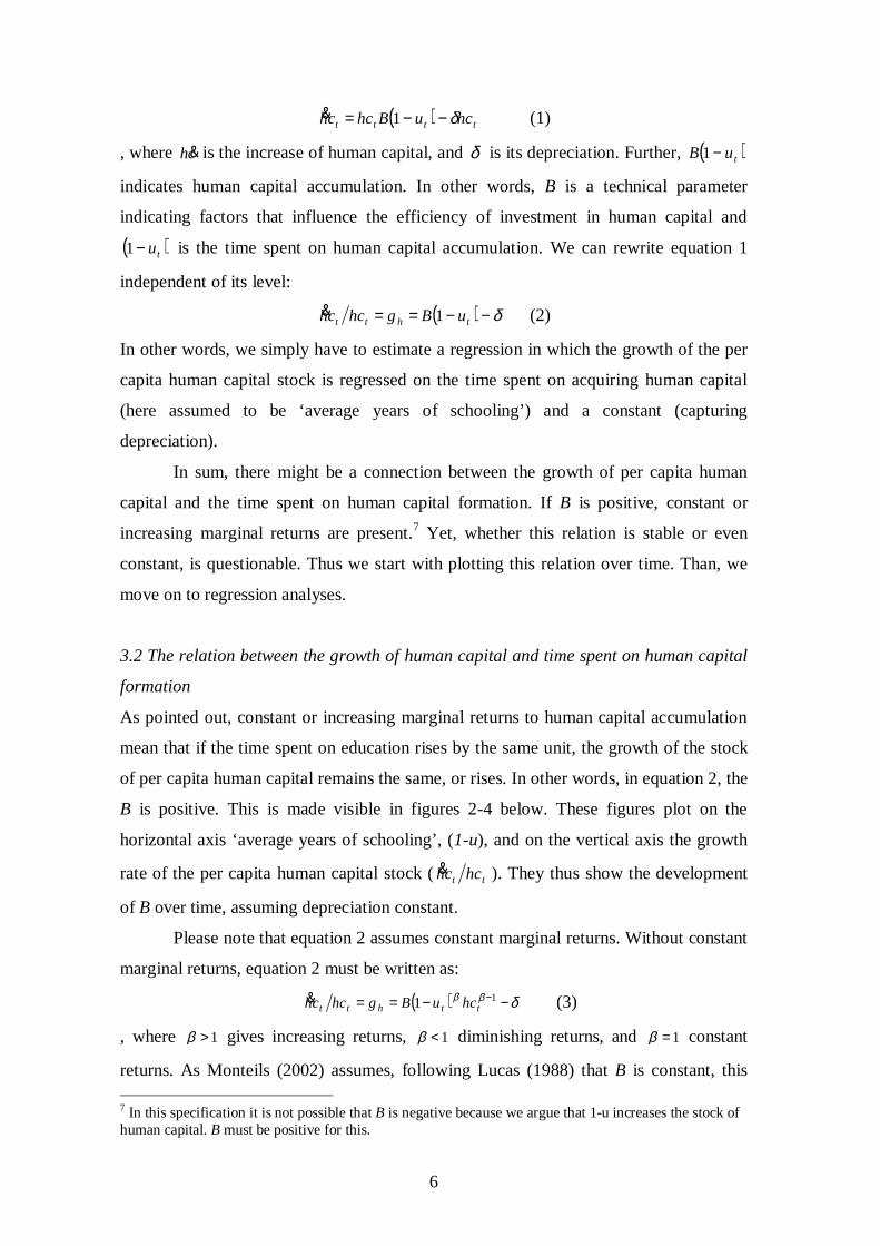
B is positive. This is made visible in figures 2-4 below. These figures plot on the
horizontal axis ‘average years of schooling’, (1-u), and on the vertical axis the growth
rate of the per capita human capital stock ( tt hcch& ). They thus show the development
of B over time, assuming depreciation constant.
Please note that equation 2 assumes constant marginal returns. Without constant
marginal returns, equation 2 must be written as:
( ) δββ −−== −11 tthtt hcuBghcch& (3)
, where 1>β gives increasing returns, 1<β diminishing returns, and 1=β constant
returns. As Monteils (2002) assumes, following Lucas (1988) that B is constant, this
7 In this specification it is not possible that B is negative because we argue that 1-u increases the stock ofhuman capital. B must be positive for this.
7
means that if the coefficient B of equation 2 decreases, this is because the relation
between (1-u) and the growth of human capital is non-linear. In other words, if she finds
a negative coefficient, this cannot be caused by decreasing efficiency (B) as this was
assumed constant, thus it must be caused by the situation that 1<β , i.e. diminishing
marginal returns. Equally, a positive coefficient would mean that 1>β , thus suggesting
increasing marginal returns. Following the line of reasoning of Monteils (2002), we
may infer that if the trend in figures 2-4 is downwards, there are decreasing marginal
returns, if it is upward, there are increasing marginal returns, and if the relation in
insignificant (a horizontal line), there are constant marginal returns to an investment in
human capital.
The figures show a remarkable pattern. Figure 2, for Japan, shows an almost
constant relation until around 5.6 years of education and a fast declining trend between
5.6 and 6.7 years of education in the population. As we move forward in time, the
‘average years of education’ also rises. So, this figure displays a development where 5.6
years of education corresponds to circa 1939 and 6.7 years to 1948. After 1975 there is
a clear upward trend.
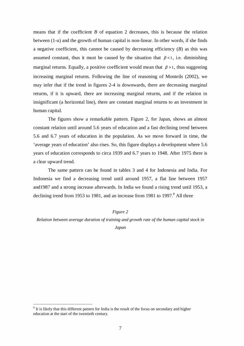
The same pattern can be found in tables 3 and 4 for Indonesia and India. For
Indonesia we find a decreasing trend until around 1957, a flat line between 1957
and1987 and a strong increase afterwards. In India we found a rising trend until 1953, a
declining trend from 1953 to 1981, and an increase from 1981 to 1997.8 All three
Figure 2
Relation between average duration of training and growth rate of the human capital stock in
Japan
8 It is likely that this different pattern for India is the result of the focus on secondary and highereducation at the start of the twentieth century.

8
-0.05
-0.03
-0.01
0.01
0.03
0.05
0.07
0.09
1 3 5 7 9 11Average years of education
Gro
wth
of t
he h
uman
cap
ital s
tock
Figure 3
Relation between average duration of training and growth rate of the human capital stock in
Indonesia
-0.02
-0.01
0
0.01
0.02
0.03
0.04
0.05
0.06
0.07
0.08
0.09
0 1 2 3 4 5 6 7 8
Average years of education
Gro
wth
of t
he h
uman
cap
ital s
tock
Figure 4
Relation between average duration of training and growth rate of the human capital stock in
India
1939
19481975
1957 1987

9
-0.06
-0.04
-0.02
0
0.02
0.04
0.06
0.08
0.1
0 1 2 3 4 5 6 7 8
Average years of education
Gro
wth
of t
he h
umna
cap
ital s
tock
countries thus show periods of decreasing, constant, and rising trends in B.9 This means
that in all three countries there are periods of increasing, decreasing, and constant
marginal returns to human capital accumulation.
3.3 Regression analyses
This interpretation is also used by Monteils (2002). Using such scatterplots and
estimating equation 2, she found strong evidence in favour of decreasing marginal
returns to human capital in France. Yet, there are two problems with her findings. First,
as indicated in the previous section, she assumes the efficiency of human capital
accumulation (B) constant. This is a strong assumption as it is often argued in the
literature that, especially for less developed countries, there was a decreasing efficiency
of human capital accumulation in the decades after World War II (Stewart 1996, 332;
Van der Kroef 1960). Second, she uses illiteracy as a measure of human capital.
Illiteracy does not pick up the complete effect of human capital, especially not for
periods when the process of increasing mass education had been completed and was
replaced by increasing secondary and higher education. Consequently, using illiteracy
data in such an analysis, one is bound to find decreasing marginal returns to human
capital accumulation.
9 Although this is an assumption which we cannot test here, we expect that the pattern of decreasing andlater increasing marginal returns to human capital formation are present in most developing countries inthe twentieth century. The reason is that they start with mass education in the first half of the twentiethcentury with generally low financial means, low quality of education, and a strong substitution of non-formal for formal education. The actual growth of the stock of human capital is thus far lower than therise in ‘average years of education’. This is different in the 1960s-1980s when those countries as well asforeign institutions strongly invested in education. Furthermore, most substitution of non-formal intoformal education had by then already taken place.
1981
1997
1953

10
In table 1, we found for India and Japan a negative coefficient of ‘average years
of schooling’ (the first regression for each country. Indeed, if we would draw a trend
line through figures 2-4, we would find a decreasing trend (and therefore decreasing
marginal returns). However, it does not decline as fast as Monteils finds for France. In
addition, we even find a positive coefficient for Indonesia. Therefore, it is clear that our
Table 1: Estimation of the marginal returns to human capital accumulation*
EXPLAINED VARIABLE, thcln∆ : Growth of human capital stock (Total human capital)
Japan Indonesia India(1) (2) (1) (2) (1) (2)
Coefficient t-value Coefficient t-
value Coefficient t-value Coefficient t-
value Coefficient t-value Coefficient t-
valueDuration of
training -0.020 -11.3 -0.028 -16.1 0.011 13.9 -0.016 -8.81 -0.010 -8.55 -0.040 -8.05
Squaredduration of
training0.001 7.71 0.003 15.2 0.003 6.22
R2 0.87 0.92 0.92 0.97 0.71 0.79
*The dummies, constant (picking up depreciation), and trend are not reported
results differ from those of Monteils (2002) mainly because we estimated a new human
capital stock that includes aspects such as the quality of human capital, thus making the
existence of constant or increasing marginal returns more likely. Indeed, we also found
in figures 2-4 that there are periods of increasing, constant, and decreasing marginal
returns for all three countries.
This finding provides some evidence against the literature that criticizes the
assumption of constant or increasing marginal returns (see for example Gong, Greiner,
and Semmler 2004; Monteils 2002). Indeed, many other authors have argued there are
good arguments for assuming constant marginal returns (Bratti and Bucci 2003; Glaeser
1994). However, we can bring this one step further as even the finding of periods with
decreasing, increasing, and constant marginal returns is subject to a problem. As
pointed out, it assumes the efficiency of human capital accumulation, B, to be constant.
Indeed, it has even been brought forward that the decrease in marginal returns causes a
decrease in efficiency (B) of the second sector (the sector in which human capital is
formed) and not by decreasing returns. For example Földvári and Van Leeuwen (2006)

11
argue that B may change, and there might be non-constant returns simultaneously. So
with a 2nd order polynomial, you capture the latter directly. 10
To capture this effect, we estimated an alternative specification, including
‘average years of schooling’ squared as suggested by Földvári and Van Leeuwen
(2006). The results are presented in table 1 (the second regression for each country).
The interpretation is simple. Taking the marginal product results in the situation that
only the coefficient of ‘average years of schooling’ squared indicates the relation
between the time devoted to human capital accumulation and human capital formation.
Only if this is positive and significant, there are increasing returns.11 Table 1 shows that
for all three countries these coefficient are positive and significant which shows that,
without the possible inefficiency, Lucasian growth would be present in all three
countries.
But is there inefficiency? Indeed, looking at figures 2-4, it is difficult to escape
the idea that technical inefficiency in the second sector plays an important role. Given
the periodization of the peaks and troughs, we expect that this decline in B is subject to
the rise in mass education as all troughs (except for Japan which developed its
education system earlier) signal periods of fast rising education levels. This can clearly
be seen in Indonesia in figure 5.12 Comparing figure 5 with 3, we see that for the period
1940-1990, when there was a fast increase in average years of education, there was a
decline in marginal returns. Or, differently, an extra input in human capital did not
10 Admittedly, rewriting this into equation 1 gives strange results. However, empirically this is the easiestway to solve the problem. If Lucas’s assumption of constant returns in the second sector holds, themarginal effect of (1-u) on the growth of HC stock equals B. Monteils (2002) estimates the equation
)1(ln uBhc −=∆ , and argues that if B decreases while (1-u) grows, there must be decreasing returns,i.e. no endogenous growth. However, this is only true if the only factor that influences the marginal effectof (1-u) on the growth of human capital has decreasing returns. This becomes different if we allow for a‘technical efficiency’ (productive efficiency in the second sector). Therefore, when we use
2)1()1( uauB −+− , the marginal effect of (1-u) on the growth of human capital becomes)1(2 uaB −+ . Thereby we decompose the observed marginal effect into two parts: an effect not directly
dependent on (1-u), denoted by B (technical efficiency), and a part which directly depends on the level of(1-u) denoted by 2a (marginal returns). If 2a is positive and significant, the larger level of (1-u) leads toincreasing growth of the human capital stock, i.e. increasing returns (endogenous growth). If 2a isnegative and significant there are decreasing returns (thus no endogenous growth, at least not withoutpositive external effects) and, if 2a is insignificant, there are constant returns (thus Lucas’s assumptionholds and this results in endogenous growth).11 As we take the marginal product of a squared variable, we have to multiply the coefficient with 2 inorder to get the actual effect of time on human capital formation. However, this does not change thefinding of the sign or significance of the coefficient.12 Here, the dip in the growth of ‘average years of schooling’ is mainly caused by the turmoil surroundingthe coup against Sukarno in the early 1960s. During this periods, many secondary schools where closed.

12
Figure 5
Growth of ‘average years of education in Indonesia, 1890-2000
-2%
-1%
0%
1%
2%
3%
4%
5%
6%
7%
8%
1890 1900 1910 1920 1930 1940 1950 1960 1970 1980 1990 2000
result in the same increase. This is also partly caused by the decrease in spending on
education that took place in that period. The average per student expenditure on
education in 1990 rupiah decreased from 156,000 in the 1930s to 28,000 in the 1950s
after which it slowly increased again. The same patterns can also be found in India. For
example, in India before 1953, the growth of ‘average years of education’ was with
2.9% smaller than the 3.2% after 1953. Equally, per student public and private
expenditure decreased from 875 constant 1990 Rupee per student in the 1930s to 569
Rupee in the 1940s. Only from the 1980s, when the marginal returns started to increase,
Figure 6
Per student private and public expenditure on education in constant 1990 yen in Japan, 1890-
2000
0
200,000
400,000
600,000
800,000
1,000,000
1,200,000
1,400,000
1,600,000
1890 1900 1910 1920 1930 1940 1950 1960 1970 1980 1990 2000

13
the per student spending again approached the level of the 1930s. In Japan, however,
the faster growth of ‘average years of schooling’ had already taken place before 1950
(2.3% versus 0.8%). Equally, in Japan there was no significant decline in per student
expenditure on education. As figure 6 shows, both before 1940 and after 1945 there was
an increase in per student expenditure, with a temporary decrease during World War II.
Thus whereas in India and Indonesia the decreasing marginal returns may be attributed
to decreasing efficiency in human capital accumulation and decreasing quality of
human capital, this was not the case in Japan.
The analysis in this section suggests three things. First, in India and Indonesia,
during a period in which the strong rise of formal education took place, it is likely the
efficiency of human capital accumulation, B, declined. Using the model of Monteils
(2002), this can result in falsely rejecting the presence of increasing marginal returns.
Second, during the strong rise of mass education after World War II, combined with
free market policies, a decline in per student government spending took place in India
and Indonesia. As increasing returns are also dependent on an increasing quality of
human capital, this makes the presence of diminishing marginal returns more likely. It
remains unclear, however, if the correction for the increase in technical inefficiency is
enough to correct for diminishing marginal returns caused by a decline in the quality of
human capital. Nevertheless, whether or not diminishing returns are present in India and
Indonesia in this period, Lucasian growth remains present as, as we noted in section 2,
the time devoted to human capital accumulation increased strongly during this period
thus creating economic growth.13 Third, neither an increase in the growth of ‘average
years of schooling’ nor a decline in the quality of human capital took place in Japan
during this period. As neither decreasing technical efficiency of human capital
accumulation nor a decline in the quality of human capital can explain the diminishing
marginal returns in the second half of the twentieth century, combined with an
accelerating economic growth, this means that no Lucasian growth was present. Or, as
we will see in table 2 in the next section, where in India and Indonesia the level of our
newly estimated human capital stock, which includes both the quantity (average years
of schooling) and the quality (expenditure on education) of human capital, will be
negatively correlated with per capita GDP growth, this relation is likely to be positive in
Japan.
13 One could also argue that these are periods of Solowian growth.

14
4. Level and growth effects of human capital
4.1 Introduction
So far, we have found some evidence which favour the theory of Lucas (1988) as an
explanation of the effect human capital has on economic growth, at least for India and
Indonesia. In Japan, however, after the 1950s, the diminishing marginal returns to
human capital accumulation could not be explained by inefficiency in human capital
accumulation or a decrease in quality of human capital. Yet, there is a second
distinction between the Lucas-Uzawa and Romer models. As pointed out in section 2,
Romer (1990) views human capital as an input in the R&D sector, thus creating
technological change. So, the level of human capital determines the rate of growth; it is
not a factor of production. Lucas (1988), on the other hand, sees human capital as a
factor of production, limited to the individual who possesses it (human capital is rival
and excludable) (Barro and Sala-i-Martin 2004). In other words, the growth of human
capital causes economic growth.
Empirically we can test the difference between the two theories by regressing
the per capita GDP growth on the level and the growth of the per capita stock of human
capital.14 If the model of Romer is correct, we expect to find a positive and significant
effect of the level of human capital on the growth of per capita GDP. But, if Lucas is
correct, we expect to find a positive and significant effect of the growth of human
capital on economic growth. Of course, these two theories are not mutually exclusive.
4.2 A standard specification: the macro-Mincer equation
We start by estimating a macro-Mincer equation. In the original micro equation, as
proposed by Mincer (1974), the log wage of a person is regressed on its education level.
And, in the original equation, age and age2 were included to capture the effect of
experience. Yet it wasn’t for long for this regression was also applied to macro-data. In
this class of regressions mostly the growth of per capita GDP was regressed on the
growth and level of the stock of human capital. Generally, GDP was used as the
14 Although this method is also used in the literature (see for example Portela et al. 2004), it is still worthnoting that Romer (1990) included human capital also as a factor of production in his specification.Therefore, in itself, the finding of a positive and significant coefficient of the growth of human capital isnot enough to dismiss the Romer model. Yet, given our previous discussion on marginal returns andgiven our finding (see table 2) that the growth of human capital has a negative coefficient in Japan and apositive one in India and Indonesia, we think that we might interpret these regressions as a test betweenthe Romer (1990) and Lucas (1988) models.

15
dependent variable because 1) it was more readily available than other possible
variables such as average wage, and 2) GDP includes not only the private effect (the
effect of human capital on own income) but also the (positive) external effect. The latter
might be important as it is possible that human capital accumulation, although the
decision to invest rests for each person solely on its private benefits, has positive
externalities. An example of such positive externalities is the transfer of ‘ideas’ and
‘techniques’ to other, non-schooled, persons on the job.
Although some criticisms have been levied against the macro-Mincer15, it is still
a relatively simple way to get a gauge of the effect of the level and of the growth of the
per capita stock of human capital. We start with a basic equation:
tttttt hchcLnyLnyktLny εββββα +∆+++∆++=∆ −−−− 14131211 lnln (4)
, where y is per capita GDP, hc is an indicator for the per capita stock of human capital
in year t, t is the trend, and ε is the error term. We used independent variables with one
time lag to avoid simultaneity.16
Equation 4 can be used to test for the difference between the theories of Romer
(1990) and Lucas (1988). If we find that the level of human capital has a positive and
significant effect on economic growth (i.e. 3β is positive and significant), this is
evidence in favour of human capital as a facilitator of technology. But, if the growth of
per capita human capital has a positive and significant impact on economic growth (i.e.
4β is positive and significant) this suggests that human capital may be viewed as a
factor of production following the theory of Lucas.
4.3 Estimation
We estimate equation 4 twice for each country using the estimated per capita stock of
human capital and ‘average years of schooling’. We include the last as comparison
15 These macro-Mincer regressions generally exclude variables indicating ‘experience’. Clearly this is aproblem. It is argued that variables as life expectancy are almost certainly related to the standard ofliving. As a consequence, inserting average experience, which is related with life expectancy, wouldcreate a simultaneity bias. This would reduce the effect of human capital on economic growth as part ofthis effect works through life expectancy (Krueger and Lindahl 2001:1109-1110). Please note that theopposite might also be true: by omitting life expectancy, the effect of human capital on economic growthmight be overestimated because part of the effect of life expectancy works through human capital. Otherworries concerning the macro-Mincer equation is that it excludes physical capital. Just as with‘experience’, excluding physical capital may cause a rise in the effect of human capital on economicgrowth.16 This means that human capital may influence growth, but growth may influence human capital as well.Admittedly, this methods, although much used in the literature, is not perfect. However, alternatives alsohave their problems. For example, the use of instrumental variables crucially depends on the choice ofinstruments. Often, time lags of the independent variables are used which are weak instruments.

16
because it is much used in the literature. We will include the newly estimated human
capital stock in the regression in logarithm and ‘average years of education’ without a
logarithm. Because of the underlying assumptions, the human capital coefficients of
both regressions will be directly comparable.17
The results are presented in table 2.18 Although giving only rough indications,
the results are striking. First we notice that for the newly estimated human capital stock
all variables of the growth of human capital are positive except Japan. But in Japan this
coefficient is only just significant at the 10% level. In the same way, when using
‘average years of education’, the coefficients of the growth of human capital are
negative. Here the exception is Indonesia, but with an insignificant coefficient. Second,
it is interesting to see that the coefficients of the level of ‘average years of education’
are positive and significant. This is not the case when using our newly estimated human
capital stock. In that case, the coefficients of the level of human capital are either
negative or positive, but in all cases insignificant.
17 Generally, studies nowadays include ‘average years of education’ in a regression (without a logarithm).We, on the other hand, also have an estimated human capital stock in monetary terms which we includein logarithmic form in the equation. So, how do we compare these two different human capitalcoefficients? First we look at why the variable ‘average years of education’ is inserted without alogarithm. This method is also advanced by, among others, Krueger and Lindahl (2001), Soto (2002), andTopel (1999), who argue that the profit in year t from human capital depends on the profit in year 0multiplied with the discount rate and the years elapsing, i.e.
( )It rhchc += 10
, where I are the number of years of education. The subscript 0 indicates that we have the initial per capitastock of human capital, for example in 1970. Now taking logarithms, we get:
( )rILnhcLnhct ++= 1ln0
Now if 0hc=α and ( )r+= 1ln3β , we can express the level of human capital asILnhct 3βα +=
Thus, if we want to estimate a regression where we want to regress the growth of per capita GDP on thelog-level of the per capita stock of human capital, we get:
ILnyt 3βα +=∆ , where I is the ‘average years of education’ and 3β indicates the elasticity (how much percent thegrowth of per capita GDP rises as I rises with 1 year). As a consequence, when taking one time lag, aboveequation is equal to equation 4 with the exclusion of the growth of human capital and the lagged y-variables, i.e. I3β corresponds to 13 ln −thcβ . This means that in both cases what the equation actuallysays is that the growth of per capita GDP depends on the log-level of the stock of human capital.18 Although this specification is much used, some problems remain. The data may exhibit breakpoints andthe equations may suffer from an omitted variable bias, mainly due to the exclusion of for examplephysical capital. Also, it might in some cases be preferable to test the validity of the inclusion of an error-correction component. Only if, after a regression between the level of per capita human capital and theappropriate error correction variable, the residual is stationary (I(0)), we are not confronted with aspurious regression, i.e. there is a cointegration relation. However, due to the long time series used anddue to the likely existence of breakpoints in the data such a regression would be useless as it wouldnormally result in a rejection of the cointegration relation. In addition, some of the data are already in firstdifferences making such a regression unnecessary as most macro-economic data are I(1).

17
Because the many problems surrounding this class of estimations we can only
present some rough conclusions based on the sign of the coefficients. Just as is
Table 2 Results from a macro-Mincer equation for India, Indonesia, and Japan 1890-2000 using per capita ‘Total HC’ and ‘average years of education’ asestimates of the growth and level of human capital**
Dependent variable: tyln∆The variable hc = total human capital The variable hc = average years of education **
India Indonesia Japan India Indonesia JapanCoefficient t-value Coefficient t-value Coefficient t-value Coefficient t-value Coefficient t-value Coefficient t-value
Constant -0.348 -2.40 0.413 2.84 0.015 0.045 0.292 1.99 0.431 2.88 0.362 5.51Trend -0.001 -1.98 0.002 3.58 0.001 0.043 -0.0001 -0.571 0.00002 0.055 -0.002 -2.16
1ln −∆ ty -0.049 -0.570 0.443 6.40 0.012 0.276 -0.074 -0.855 0.394 5.67 0.018 0.454
1ln −ty -0.015 0.831 -0.070 -3.48 -0.043 -2.32 -0.047 -1.92 -0.064 -2.85 -0.058 -5.80
1ln −∆ thc 0.015 0.084 1.096 2.85 -0.423 -1.69 -0.040 -1.29 0.006 0.065 -0.027 -0.689
1ln −thc -0.047 0.015 -0.008 -0.798 0.036 1.30 0.020 3.95 0.015 2.31 0.039 4.85
R2 0.408 0.711 0.849 0.364 0.703 0.876Obs. 109 110 106 109 107 110AR1-1 (prob) 0.712 0.199 0.280 0.172 0.271 0.961Normality(prob) 0.549 0.070 0.381 0.997 0.154 0.050
*Dummies not reported**‘average years of education’ is inserted in the equation without logarithms.
commonly argued in the literature, we found that the coefficient of the level of ‘average
years of education’ is positive, significant, but small, being between 1.5% and 4%.
Combined with a generally insignificant effect of the coefficient of the growth of
‘average years of education’ this explains why most studies end up favouring the
interpretation of Romer. Yet, this can be attributed to omitting the rises in quality of the
human capital stock (see Behrman 1983, and our discussion in the previous section).
This results in diminishing returns and thus a rejection of the Lucas-Uzawa model.
However, looking at the regressions with our newly estimated human capital stock, we
found, except Japan, a positive effect of the growth of human capital on per capita GDP
growth (for Indonesia this effect was even significant at 10%) while the effect of the
level was insignificant for India and Indonesia. For Japan, although not significant at
the 10% level, the t-value of the level of human capital still exceeded one, which, as a
rule of thumb, means that this variable is important for explaining economic growth.
These regressions seem to confirm our findings from section 3. India and
Indonesia had a positive effect of the growth of human capital (although not significant
for India), thus pointing into the direction of Lucasian growth. The decline in the
marginal returns found for Indonesia and India in the previous section thus can thus

18
largely be explained by a decreasing technical efficiency, (B), and a decreasing per
student expenditure as an indicator of the quality of human capital. Japan, however,
experienced a positive effect of the level of human capital. This points in the direction
of Romerian growth, at least in the period after the 1950s when the marginal returns to
human capital accumulation started to decrease strongly.
5. Connecting level and growth effects with constant marginal returns to human
capital accumulation
We saw that in table 2, with the exception of Japan, both the level of ‘average years of
schooling’ and the growth of the newly estimated human capital stock had a positive
effect on the growth of per capita GDP. This means that if the growth of human capital
determines economic growth while it is the level of ‘average years of education’ that
affects economic growth, the level of ‘average years of education’ must determine the
growth of the newly estimated stock of human capital. This is easy to see. We start with
hcch
yy &&
βα += (5)
, where the growth of per capita GDP depends on the growth of the per capita estimated
human capital stock. This is roughly the equation describing the long-run growth in the
model of Lucas (1988). However, if we look at the level of ‘average years of
schooling’, we get:
educyy
ϕγ +=& (6)
, where educ, the level of ‘average years of schooling’, determines the growth of per
capita income. This is the regression following from the theory of Romer (1990).
However, combining equation 5 and 6 leads to:
hccheduc
&βαϕγ +=+ (7)
, which can be rewritten in the following fashion:
educhcch
βϕ
βγα
+−
=&
(8)
Therefore, the growth of human capital depends on the level of ‘average years of
schooling’. If we , as we have done in section 3, see ‘average years of schooling’ as a
proxy for the time devoted to human capital accumulation, we end up with exactly what
Lucas argues to be the main source of endogenous growth: constant (or increasing)

19
marginal returns to human capital accumulation which is present in India and Indonesia.
Completing this way of thinking, one may (somewhat exaggerating) argue that studies
that find evidence in favour of Romer’s theory from regressions based on average years
of schooling as a proxy for human capital, basically confirmed Lucas’ theory without
being aware of it (see for example Benhabib and Spiegel 1994; Krueger and Lindahl
2001; Portela et al. 2004).
6. Some suggestive interpretations of economic growth
6.1 A successful developer: Japan
From figure 2 it seems there are constant marginal returns to human capital
accumulation in Japan until around 1939 and diminishing returns afterwards. This
implies Lucasian growth in the first half of the twentieth century. However, after 1939,
there has been a turn to Romerian growth. An important indication are our findings in
table 2 where, contrary to India and Indonesia, the level of human capital has a positive
effect on economic growth as is the case in the Romer (1990) model.
But why took this shift place in Japan and not in India and Indonesia? We
distinguish four points. A first point is that the efficiency of the education system was
higher in Japan than it was in India and Indonesia. Education better connected to society
and economy in Japan than was the case in India and Indonesia. Though, besides the
ideal of creating a strong state, economic and social developments led to educational
development in Japan after the Meiji restoration in 1868, in India and Indonesia, as in
most developing economies, it were largely ideas of ‘creating an indigenous class of
literati’, a ‘moral duty of the colonizer country’, nationalism, and, after World War II,
the ‘idea of progress by education’, ‘lack of finances’, and ‘policies of international
organisations’ that drove their educational development. In other words, it were often
global, or at least external, factors that influenced the education systems of India and
Indonesia (Ramirez and Boli 1987, 10; Stewart 1996).
The differences in the efficiency of the education systems have three results. First,
being a technical problem, in section 3 we noted inefficiency (in B) in the second sector
to be present in India and Indonesia in the mid-twentieth century. Given the test used,
this caused diminishing marginal returns to human capital accumulation. Yet, after
correcting for inefficiency in B, we found increasing marginal returns. But no such
inefficiency seems to be present in Japan. Thus we cannot argue, as we did for India
and Indonesia, that other factors caused the diminishing returns and that Lucasian

20
growth remained present. Second, because Japan experienced a more economy centred
development, its education system started to develop earlier than was the case in India
and Indonesia. This we also see in figure 1 where the per capita stock of human capital
of Japan around 1900 far exceeds those of India and Indonesia. Because Japan already
had a far higher education level around 1950, further educational growth was unlikely
to be accompanied by constant marginal returns. For example, if there are already 10
teachers for each student, to add an eleventh teacher will not add much to human capital
accumulation. Third, a better educational development also raised income, especially
because there was a closer connection between human capital and the labour market. A
higher income a head in turn created the opportunity to keep expanding educational
spending even in the 1950s and 1960s. So, whereas India and Indonesia where trapped
in vicious cycles of low per student spending and fairly low growth, Japan was in a
virtuous cycle with high growth and fast rising educational spending. Therefore, Japan
did not only develop earlier but also faster in education.
This brings us to the second point why Japan experienced a shift from Lucasian
to Romerian growth. It is likely that, because Japan developed earlier and faster, it did
not have to face constraints that were present for later developers. As pointed out in
section 2, Lucasian growth implies human capital accumulation. But this can also affect
economic growth through adopting (foreign) technologies. As has been argued by
O’Neill (1995, 26), the level of education causes convergence among countries.
However, this convergence is reversed for developing countries by human capital
biased technological growth, which increases the rate of returns for higher education
and thus favours the developed world. In other words, technology causes growth.
Because technological development nowadays requires secondary and higher education,
in which the developed countries have a relative advantage, developed countries profit
more from new technologies than do developing countries. Japan, however, is clearly
ahead in education development compared with India and Indonesia. In 1950 the
average years of schooling in Japan was 6.9 years against 1.8 in India and 1.5 in
Indonesia.
Third, unlike India and Indonesia, Japan had an educational development large
enough to create an extensive manufacturing sector. Initially Japan witnessed a dual
economy where artisan industries coexisted with modern industries. This caused an
equal division of wages and thus of educational development. This combination of
artisan with modern industries was special for Japan compared to India and Indonesia.

21
This is combined with the situation that Japanese agriculture is labour intensive because
of the small plots of land (Buchanana 1923, 550). Many of those professions without
land such as blacksmiths, day workers, or cotton mill workers, were filled as
agricultural by-employment. As an effect, wages in these professions remained almost
equal to farm wages. Therefore, the growth of manufacturing was possible by low
wages and a high availability of skills, which in turn created the opportunity to acquire
more technology (Mayer 2001, 19).
Because of the technological and human capital development, as a fourth point
Japan came increasingly closer to the technological frontier. The government sponsored
industrialisation and rising skill levels caused a separation of not only factory industry
but also artisan industries from agriculture. As a result, wages diverged and the demand
for higher skills became more pronounced. For example, as a rule only those who have
finished the six year elementary course were employed at the mills (National
Confederation of Industrial Associations of Japan 1937, 7). This made it preferred to
create new technologies to reduce the wage bill and increase productivity. This
approach of a threshold level is also acknowledged by Kim and Oh (1999, 13) when
they argue that “[f]or economies in which government take initiatives for industrial
development, their lion share of resources is usually allocated to strengthen the supply
side of technology, such as training manpower, supporting basic science, and
establishing public R&D institution. (…) Once their accumulated level of capability
reaches a certain level of supply, (…) then the demand for technology will be motivated
indigenously.” They find that Japan had passed this threshold level in the second half of
the twentieth century.
6.2 Late-comers in economic development: India and Indonesia
In India and Indonesia Lucasian growth seems to be present over the entire twentieth
century. Figures 3 and 4 show for both countries extended periods of increasing and
diminishing marginal returns. But table 2 in section 4 shows a positive effect of the
growth of human capital, suggesting Lucasian growth. Also, regression 2 in table 1
showed that in a primitive way correcting for inefficiency in human capital
development results in the removal of diminishing marginal returns. This suggests that
either there were no periods with diminishing marginal returns or the periods that were
present did not mark an end to Lucasian growth as was the case in Japan.

22
But why was this the case? First, using the Monteils (2002) model, just as in
Japan there are troughs in the marginal returns. But unlike Japan, this can be explained
by increasing inefficiency in human capital formation (B). Second, the quality of human
capital in the 1950s and 1960s decreases. This process, which is common among
developing economies, is caused by a large rise in government spending on education,
replacing private expense, and global policies that favour market forces to cause
educational development. Combined with a lack of financial means, this leads to low
per student investment in education (Stewart 1996; Tilak 1984).
Third, as we argued in section 6.1, in Indonesia and India human capital is only
loosely connected to the labour market. For example, in Indonesia before Independence,
there was a dual educational structure for Indonesians and Europeans. Yet, it was
difficult for educated Indonesians to enter the labour market. Indonesian enterprises
were largely artisan and, as a result, not so much suited for educated Indonesians. As an
effect, educated Indonesians were almost entirely working in the Government sector
and the remainder in the European industries. Only a few were self-employed or had
jobs in Indonesian enterprises. This vision is confirmed in a report about the metal
industry at Surabaya in 1926. This industry was largely European, but employed many
Indonesians. Of these Indonesians there are data about their education level, not only of
western but also of Indonesian education (see table 3). Interestingly, we see that a low
level of about 7% of the Indonesian employees was educated. We also see that from this
7% by far the largest share had been enrolled in Indonesian education. Because the
Table 3: Indigenous employees in the metal industryin Soerabaja in 1926*
Education level % employees
No education 92,6%Indonesian primary school 5,4%European primary school 0,7%Dutch-Indies school 0,6%K.E.S. Secondary technical school 0,0%Indonesian vocational school 0,1%Burgeravondschool 0,2%Other schools 0,3%* 28 enterprisesSource: A.G. Vreede (1926, 10)
metal industry demanded a fairly high education, this figure is higher than it would be
for most other industries. Therefore, it is not likely that Western, or Indonesian

23
education for that matter, for Indonesians was a way to develop the indigenous
economy (Hollandsch-Inlandsch onderwijs-commissie 1930, 26).
Fourth, Lucasian growth means that productivity per employee grows if human
capital grows. This can be reached by adopting new technologies. But, clearly, India
and Indonesia lagged behind the western countries and Japan. This makes it difficult to
adopt new technologies, not only because technology is often biased toward higher
education in which developed countries often have a comparative advantage (see
O’Neill 1995), but also because it is often politically difficult to modernize as this will
cause social unrest.19 An interesting example can be found in textiles in India and
Indonesia. In India, caused by high wages, labour unrest, taxation policy, and
bureaucratic control, it were the handloom weavers and the small powerloom operators
that experienced rapid growth during the 1960s while the larger-scale sector (textile
mills, mainly found in the metropolitan areas) declined. Wages in mills, for example,
could be up to three times as high compared with more modern powerloom operators
(RoyChowdhury 1995, 233). In the mid 1980s more market forces were let in but this
did not reverse the trend. The same was true in Indonesia where the textile industry,
which had known already a large growth after the 1930s partly because of a protective
policy of the colonial government, continued to grow under the same policy after
independence. Because the lack of competition, however, the number of powerlooms,
even after independence, remained small compared with handlooms. At the end of the
1950s and the start of the 1960s this industry was using only some of its capacity.
Problems were the shortage of spare parts, lack of skilled labour, and especially the
shortage of raw material (raw cotton and yarn) (Palmer and Castles 1965, 41). This was
because the spinning industry could not supply enough yarn. And, much yarn, imported
by the State Trading Corporations, was sold on the free market, reducing its availability.
Also, the yarn that did enter the producers’ hands direct through quota had to be paid
for in advance. Many smaller producers could not pay the quota and gained it by
working for intermediaries who paid the quota, or through selling their quota to larger
and more efficient producers. In this way the larger producers got more raw materials
(Palmer and Castles 1965, 43). Under Sukarno’s licensing system it was thus profitable
to have a license for a loom even though it was a handloom. Then you could obtain a
quotum of yarn, which could be sold to larger and more efficient producers (Boucherie
19 For example, Clark (1987, 168-169) argues that the local environment has a strong influence onwhether workers are willing to adopt more or different machines.

24
1969, 55). This allocation system was abolished in 1967 and the channelling of yarn
was left to market forces. Nevertheless, productivity rose slowly, even in the modern
(powerloom) sector. In the larger factories that could have had economies of scale there
were old looms often from the 1930s and 1940s while the smaller factories used more
modern looms but had no economies of scale (Boucherie 1969, 58). These two
examples suggest that political and technological barriers for later developers could be
an important reason of lower efficiency and growth in these countries.
But there is also a fifth reason these countries suffer from lower growth. Barro
and Sala-i-Martin (2004) intuitively developed an imbalance effect of the stocks of
human and physical capital in the Lucas model. When the ratio of physical to human
capital exceeds the equilibrium ratio (there is too much physical relative to human
capital), economic growth declines. When the ratio of physical to human capital rises
(there is too much human relative to physical capital), economic growth increases.20 If
one wants to increase economic growth, it is thus preferable to have an excess of human
capital. But an excess of either human- or physical capital reduces the returns of the
abundant factor and therefore more will be invested in the scarce factor. Yet, whether
countries can get a growth bonus in this way is also dependent on technology. If
technology is labour biased, which it usually is, then in countries where the elasticity of
substitution between skilled and unskilled labour is small, the price effect dominates
and technology is directed at the scarce factor of production. That is, if human capital is
abundant relative to physical capital, technology is directed at unskilled labour and vice
versa. But in countries with a high elasticity of substitution, the market effect dominates
and technology is directed toward the abundant factor (Acemoglu 2002).
As pointed out, countries with a higher educational development (and a higher
economic development) show Romerian growth which does not know an imbalance
effect. Indeed, if we, like Grandville (1989, 479), see the elasticity of substitution as ‘a
measure of the efficiency of the productive system’, we may argue that countries with a
lower efficiency of human capital (or a less strong connection between human capital
and the economy) suffer from a low elasticity between skilled labour (as a measure of
human capital) and unskilled labour. So, it is likely that developed countries have a
20 Empirically it is also possible that in both cases economic growth increases.

25
higher elasticity21, but as we have seen for Japan, are in a phase of Romerian growth
where this imbalance effect is of less importance.
This has the interesting result for developing economies that, when there is an
excess supply of physical capital, technology is focused at skilled labour (which is the
scarce component in the relation between skilled and unskilled labour). This increases
the productivity of skilled labour, increasing its returns, and thus slows down
investments in human capital to arrive again at the equilibrium ratio of human to
physical capital. Conversely, if there is an excess supply of human capital, technology
will again be directed at the scarce factor (unskilled labour). As physical capital is not
necessarily solely embodied in unskilled labour, there is no reason investments in
physical capital are slowed down. Therefore, in countries with a low elasticity of
substitution, adapting to the equilibrium ratio from an excess supply of human capital
will be faster than from an excess of physical capital. As the former increases growth
while the second reduces it, the overall long-run effect will be negative. In other words,
a low elasticity of substitution between skilled and unskilled labour as is likely to be
found in developing economies causes a decline of their steady state growth because the
positive effects of the imbalance effect are outweighed by the negative effects.22
7. Conclusion
In this paper we tried to apply the two main branches of the new growth theories on the
economic development of three countries that were initially for a large part dependent
on adopting education and technology: India, Indonesia, and Japan. But where the latter
proved successful, the former two lagged behind.
We tried to use two formal tests to find out which growth theory best described
the link between human capital and economic growth. We distinguished two classes of
endogenous growth theories. First, there is the model of Romer (1990) where human
capital is seen as a factor facilitating R&D and in this way increasing technological
growth. Second, there is the theory of Lucas (1988) who sees human capital as a factor
21 A low elasticity of substitution seems to be especially prevalent in developing economies. We foundthat the elasticity between the skill premium and the skilled wage (and as a consequence the elasticitybetween the unskilled and skilled labour) was much higher in Japan than in India and Indonesia.However, elasticities above 1.4 between skilled and unskilled wage (between high school and collegelabour) were also found for the United States, Canada, and the United Kingdom by Katz and Murphy(1992: 72) and Card and Lemieux (2001: 734).22 Indeed, that a higher elasticity of substitution may increase steady state growth is also argued, for theSolow model, by Rainer Klump and Harald Preissler (2000). The main difference is that we argue that itworks through the imbalance effect.

26
of production. We used this difference to test the applicability of each theory to
economic growth.
The first test, following Monteils (2002), is based on the situation that in the
theory of Lucas there are two sectors. In the first sector, human capital is used to
produce output while in the second sector human capital is used to create new human
capital. Therefore, if one ignores positive external effects of human capital, endogenous
growth can only be possible if there are constant or increasing marginal returns to
human capital accumulation. We found extended periods with constant or increasing
marginal returns. This evidence supports the applicability of the Lucasian growth. If
efficiency in the second sector has the shape of a trough parabola, we found for all three
countries increasing returns. However, though rising growth of ‘average years of
schooling’ and a decreasing quality of human capital can explain the diminishing
marginal returns in India and Indonesia, this cannot provide an explanation for Japan in
the second half of the twentieth century. Therefore, though India and Indonesia suffered
from periods with increasing, constant, and diminishing marginal returns without
leaving the phase of Lucasian growth, Japan moved from Lucasian growth in the first
half of the century to Romerian growth in the second half.
This was confirmed in the second test. Here we regressed the growth of per
capita GDP on the level and growth of per capita human capital. Given that Lucas
(1988) saw human capital as a factor of production, the growth of human capital should
have a positive influence on economic growth. As Romer saw human capital only as an
input in the R&D sector, in his theory the level of human capital should have a positive
effect on economic growth. Our regressions resulted, except for Japan, in positive
coefficients of the growth of human capital and insignificant coefficients of the level
thus suggesting Lucasian growth. In Japan, with a positive coefficient of the level of
human capital, there are strong signs of Romerian growth in the twentieth century.
Why did Japan move from Lucasian to Romerian growth and India and
Indonesia not? We attributed this to four causes. First, in India and Indonesia, the
education systems were less connected to the economy and thus less efficient. Second,
the quality of human capital, measured as total per student spending on education,
decreased strongly in the mid-twentieth century. Third, because Japan developed earlier
obstacles in acquiring technologies were less pronounced. We referred to economic
obstacles (a bias of technology to higher education in which developed countries have a
comparative advantage) and political obstacles (institutions and policies that are

27
harmful for technological modernisation). Fourth, in developing countries, technologies
may be biased toward the scarce factor of production. In combination with an
imbalance effect caused by Lucasian growth, this may in some cases result in an on
average negative effect on steady state growth.
ReferencesAcemoglu, Daron, ‘Directed technical Change,’ Review of Economic Studies, Vol. 69 (4) 2002, 781-810.Barro, Robert J. and Xavier Sala-i-Martin, Economic Growth, Cambridge and London: The MIT Press
2004.Behrman, Jere R. and Nancy Birdsall, ‘The Quality of Schooling: Quantity Alone is Misleading,’ The
American Economic Review, Vol. 73 (5) 1983, 928-946.Benhabib, J. and M. Spiegel, ‘The role of human capital in economic development: evidence from
aggregate cross-country data,’ Journal of Monetary Economics, Vol. 34 (2) 1994, 143-174.Boucherie, W., ‘The Textile Industry,’ Bulletin of Indonesian Economic Studies, Vol. 5 (3) 1969, 47-70.Bratti, Massimiliano and Alberto Bucci, ‘Human Capital and International Differences in Income
Levels,’ Paper presented at the workshop ‘Economic Growth and Income Distribution’ inAncona 2003.
Buchanana, Daniel H., ‘The Rural Economy of Japan,’ The Quarterly Journal of Economics, Vol. 37 (4)1923, 545-578.
Card, David, and Thomas Lemieux, ‘Can Falling Supply Explain the Rising Return to College forYounger Men? A Cohort-Based Analysis,’ The Quarterly Journal of Economics, Vol. 116 (2)2001, 705-746.
Clark, Gregory, ‘Why Isn’t the Whole World Developed? Lessons from the Cotton Mills,’ The Journal ofEconomic History, Vol. 47 (1) 1987, 141-173.
Eng, Piere van der, ‘The Real Domestic Product of Indonesia, 1880-1989,’ Explorations in EconomicHistory, Vol. 28 (3) 1992, 343-373.
Földvári, Péter, and Bas van Leeuwen, ‘Economic growth in Three Worlds’ Paper presented at theEuropean Social Science History Conference (ESSHC), Amsterdam 2006.
Glaeser, Edward L., ‘Why Does Schooling Generate Economic Growth?’ Economic Letters, Vol. 44(1994), 333-337.
Gong, Gang, Alfred Greiner, and Willi Semmler, ‘The Uzawa-Lucas Model Without Scale Effects:Theory and Technical Evidence,’ Structural Change and Economic Dynamics, Vol. 15 (2004),401-420.
Grandville, O. de la, ‘In Quest of the Slutzky Diamond,’ American Economic Review, Vol. 79 (1989),468-481.
Hollandsch-Inlandsch onderwijs-commissie, De werkgelegenheid in Nederlandsch-Indie voorNederlandsch sprekenden, (Rapport 6a) Weltevreden: Landsdrukkerij 1930.
Katz, Lawrence F., and Kevin M. Murphy, ‘Changes in Relative Wages, 1963-1987: Supply and DemandFactors,’ The Quarterly Journal of Economics, Vol. 107 (1) 1992, 35-78.
Kibritcioglu, A. and S. Dibooglu, ‘Long-run Economic Growth: An Interdisciplinary Approach,’ Officeof Research Working Paper No. 01-0121, University of Illinois 2001(http://www.business.uiuc.edu/Working_Papers/papers/01-0121.pdf )
Kim, Sun G., and Wankeun Oh, ‘The Relation between Government R&D and Private R&D Expenditurein the APEC Economies: A Time Series Analysis,’ KIEP Working Paper 99-22, Korea Institutefor International Economic Policy 1999.
Klump, Rainer, and Harald Preissler, ‘CES Production Functions and Economic Growth,’ ScandinavianJournal of Economics, Vol. 102 (1) 2000, 41-56.
Kroef, Justus M. van der, ‘The Educated unemployed in Southeast Asia: A Common Problem in India,Indonesia, and the Philippines,’ Journal of Higher Education, Vol. 31 (4) 1960, 177-184.
Krueger, Alan B., and Mikael Lindahl, ‘Education for Growth: Why and For Whom?,’ Journal ofEconomic Literature, Vol. 39 (4) 2001, 1101-1136, 1114.
L’Angevin, Clotilde, and Nadine Laïb, ‘Education and Growth in a Panel of 21 OECD Countries,’International Conference on Policy Modelling, Istanbul 2005.
Lucas, Robert, ‘On the Mechanics of Economic Development,’ Journal of Monetary Economics, Vol. 22(1) 1988, 3-42.
Maddison, Angus, The World Economy: Historical Statistics, Paris: OECD 2003.Mayer, Jörg, ‘Technology diffusion, human capital and economic growth in developing countries,’

28
United Nations Conference on Trade and Development, Discussion Papers No. 154, 2001.Mincer, J., ‘Schooling, Experience and Earnings,’ NBER, New York 1974.Monteils, Marielle, ‘Education and Economic growth: Endogenous Growth theory Test. The French
Case,’ Historical Social Research, Vol. 27 (4) 2002, 93-107.National Confederation of Industrial Associations of Japan, Industrial Relations in Japan: Characteristic
measures for workers’ welfare in silk and cotton mills, Tokyo: National Confederation ofIndustrial Associations of Japan 1937.
OECD, The Well-being of Nations: The Role of Human and Social Capital, Paris: OECD 2001.O’Neill, Donal, ‘Education and Income Growth: Implications for Cross-country Inequality,’ The Journal
of Political Economy, Vol. 103 (6) 1995, 1289-1301.Palmer, Ingrid, and Lance Castles, ‘The Textile Industry,’ Bulletin of Indonesian Economic Studies, Vol.
1 (2) 1965, 34-48.Portela, Miguel, Rob Alessie, and Coen Teulings, ‘Measurement Error in Education and Growth
Regressions,’ Tinbergen Institute Discussion Paper, TI 2004-040/3, 2004.Ramirez, Francisco O., John Boli, ‘The Political Construction of Mass Schooling: European Origins
and Worldwide Institutionalization,’ Sociology of Education, Vol. 60 (1) 1987, 2-17.Rebelo, Sergio T., ‘Long Run policy Analysis and Long Run Growth,’ Journal of Political Economy,
Vol. 99 (3) 1991, 500-521.Romer, P., ‘Endogenous Technological Change,’ Journal of Political Economy, Vol. 98 (5), part 2 1990,
71-102.Roy, Bina, An Analysis of Long term growth of National Income and Capital Formation in India (1850-
51 to 1950-51), Calcutta: Firma KLM Private Limited 1996.RoyChowdhury, Supriya, ‘Political Economy of India’s Textile Industry: The Case of Maharashtra,
1984-89,’ Pacific Affairs, Vol. 68 (2) 1995, 231-250.Sianesi, Barbara and John Van Reenen, ‘The Returns to Education: Macroeconomics,’ Journal of
Economic Surveys, vol. 17 (2) 2003, 157-200.Solow, R.M., ‘A Contribution to the Theory of Economic Growth.’ Quarterly Journal of Economics, Vol.
70 (1) 1956, 65-94.Soto, Marcelo, ‘Rediscovering Education in Growth Regressions,’ Working Paper No. 2020, OECD
Development Centre 2002.Stewart, Frances, ‘Globalisation and education,’ International Journal of Educational Development, Vol.
16 (4) 1996, 327-333.Tilak, Jandhyala B.G., ‘Political Economy of Investment in South Asia,’ International Journal of
Educational Development, Vol. 4 (2) 1984, 155-166.Topel, Robert, ‘Labor Markets and Economic Growth,’ in: Handbook of Labour Economics, Orley
Ashenfelter and David Card (eds.), Amsterdam: North Holland 1999.Uzawa, Hirofumi, ‘Optimum Technical Change in an Aggregate Model of Economic Growth,’
International Economic Review, Vol. 6 (1) 1965, 18-31.Vreede, A.G., Rapport van het Hoofd van het Kantoor van Arbeid over de arbeidstoestanden in de
metaalindustrie te Soerabaja, Publicaties van het Kantoor van Arbeid; No. 1, Weltevreden:Landsdrukkerij 1926.