The Role of Genomic Copy Number Variation (CNV) in ... · The Role of Genomic Copy Number Variation (CNV) in Osteoporosis Kate Connolly Bachelor of Forensics and Bachelor of Science

The Role of Genomic Copy Number Variation (CNV) in Osteoporosis

Kate Connolly Bachelor of Forensics and Bachelor of Science (Triple Major)

School of Biological Sciences and Biotechnology Murdoch University

2012

Principle Supervisor: A/Professor Scott Wilson

Department of Endocrinology and Diabetes Sir Charles Gairdner Hospital

Co-Supervisor: Professor Roger Price

Department of Endocrinology and Diabetes Sir Charles Gairdner Hospital

Responsible Academic: A/Professor Robert Mead School of Biological Sciences and Biotechnology

Murdoch University

This thesis was submitted in partial fulfilment of the requirements for the award of Honours Degree in Molecular Biology at Murdoch University, Western Australia

i

Table of Contents

TABLE OF CONTENTS ......................................................................................................................................... I

DECLARATION ................................................................................................................................................ IV

ACKNOWLEDGEMENTS ................................................................................................................................... V

LIST OF ABBREVIATIONS ................................................................................................................................ VI

INDEX OF FIGURES ......................................................................................................................................... IX

INDEX OF TABLES ............................................................................................................................................ X

ABSTRACT ..................................................................................................................................................... XII

CHAPTER 1: INTRODUCTION ............................................................................................................................ 1

1.1 THE IMPACT OF OSTEOPOROSIS ................................................................................................................. 2

1.2 THE OSTEOPOROTIC DISEASE PROCESS ...................................................................................................... 5

1.2.1 BONE BIOLOGY .............................................................................................................................................. 5

1.2.1.1 Bone Remodelling .............................................................................................................................. 5

1.2.1.2 Bone Regulation ................................................................................................................................. 6

1.2.2 PRIMARY RISK FACTORS FOR OSTEOPOROSIS ....................................................................................................... 8

1.3 EARLY INTERVENTION OF OSTEOPOROSIS ............................................................................................... 10

1.3.1 DETECTION OF FRACTURE RISK VIA BMD .......................................................................................................... 10

1.3.2 PREVENTION OF OSTEOPOROSIS ...................................................................................................................... 11

1.4 THE GENETIC CONTRIBUTION TO OSTEOPOROSIS .................................................................................... 13

1.4.1 COMMON COMPLEX PATTERN OF INHERITANCE ................................................................................................. 13

1.4.2 IDENTIFICATION OF GENETIC FACTORS THAT ARE ASSOCIATED WITH DISEASE............................................................ 14

1.4.3 EVIDENCE SUPPORTING THE HERITABILITY OF OSTEOPOROSIS ................................................................................ 16

1.5 HUMAN GENETIC VARIATION .................................................................................................................. 18

1.5.1 FUNCTIONAL CONSEQUENCE OF HUMAN GENETIC VARIATION .............................................................................. 19

1.5.1.1 Transcriptional Control of Gene Expression ..................................................................................... 19

1.5.2 CHARACTERISATION OF HUMAN GENETIC VARIATION .......................................................................................... 21

1.5.2.1 Single Nucleotide Polymorphisms (SNPs) ......................................................................................... 22

1.5.2.2 Structural Variation .......................................................................................................................... 23

1.6 COPY NUMBER VARIATION (CNV) ............................................................................................................ 25

1.6.1 MECHANISM OF CNV FORMATION .................................................................................................................. 25

1.6.2 FUNCTIONAL CONSEQUENCE OF CNV ............................................................................................................... 26

1.6.3 CNVS AND DISEASE ...................................................................................................................................... 27

1.7 STATEMENT OF THESIS ............................................................................................................................. 30

1.7.1 GENERAL PURPOSE OF RESEARCH .................................................................................................................... 30

1.7.2 HYPOTHESIS ................................................................................................................................................ 30

1.7.3 AIMS OF STUDY ............................................................................................................................................ 30

CHAPTER 2: MATERIALS AND METHODS ........................................................................................................ 32

2.1 MATERIALS .............................................................................................................................................. 33

ii

2.1.1 SELECTION OF CNVS FOR STUDY ..................................................................................................................... 33

2.1.2 GDNA PREPARATION .................................................................................................................................... 33

2.1.3 QPCR (REAL-TIME QUANTITATIVE POLYMERASE CHAIN REACTION) ....................................................................... 34

2.1.4 ANALYSIS OF EXPERIMENTAL DATA .................................................................................................................. 35

2.1.5 GENERAL LABORATORY PROTOCOL .................................................................................................................. 35

2.2 METHODS ................................................................................................................................................ 36

2.2.1 SELECTION OF CNVS FOR STUDY ..................................................................................................................... 36

2.2.1.1 Identification of Potential Osteoporosis Genes ................................................................................ 36

2.2.1.2 Identification of CNVs ...................................................................................................................... 37

2.2.1.3 Critical Evaluation of CNVs ............................................................................................................... 38

2.2.2 SAMPLE PREPARATION .................................................................................................................................. 39

2.2.2.1 Study Subjects .................................................................................................................................. 39

2.2.2.2 gDNA Dilution .................................................................................................................................. 40

2.2.3 DETECTION OF CNV ...................................................................................................................................... 41

2.2.3.1 Overview of qPCR ............................................................................................................................. 42

2.2.3.2 Overview of TaqMan Assay Detection Chemistry ............................................................................ 43

2.2.3.3 Selection of TaqMan Assays used in Study....................................................................................... 44

2.2.3.4 CNV Genotyping via qPCR ................................................................................................................ 47

2.2.4 QUANTITATION OF CNVS ............................................................................................................................... 48

2.2.4.1 Overview of CopyCaller .................................................................................................................... 48

2.2.5 CRITICAL EVALUATION OF EXPERIMENTAL DATA ................................................................................................. 51

2.2.5.1 Tests of Reliability and Reproducibility ............................................................................................ 51

2.2.5.2 Prioritisation of Samples with ‘Unconfirmed’ CN from First Round of Genotyping ......................... 52

2.2.5.3 Prioritisation of Samples with ‘Unconfirmed’ CN from Second Round of Genotyping ..................... 53

2.2.6 STATISTICAL ANALYSIS OF EXPERIMENTAL DATA ................................................................................................. 54

2.2.6.1 Consolidation of Genotype and Phenotype Data ............................................................................. 54

2.2.6.2 Tests of Normality via SPSS .............................................................................................................. 55

2.2.6.3 Tests of Association via SPSS ............................................................................................................ 56

CHAPTER 3: ANALYSIS OF ESR1 CNV AND BMD .............................................................................................. 59

3.1 INTRODUCTION ........................................................................................................................................ 60

3.2 MATERIALS AND METHODS ..................................................................................................................... 66

3.3 RESULTS ................................................................................................................................................... 67

3.3.1 QUALITY CONTROL ....................................................................................................................................... 67

3.3.2 CNV GENOTYPE FREQUENCY DISTRIBUTIONS ..................................................................................................... 68

3.3.3 SPSS TESTS OF NORMALITY ........................................................................................................................... 69

3.3.3.1 ESR1 CNV and Raw BMD Measurements (g/cm2) ............................................................................ 69

3.3.3.2 ESR1 CNV and Age-Adjusted BMD Z-Scores ..................................................................................... 73

3.3.4 ASSOCIATION ANALYSIS ................................................................................................................................. 76

3.3.4.1 ESR1 CNV and Raw BMD Measurements (g/cm2) ............................................................................ 76

3.3.4.2 ESR1 CNV and Age-Adjusted BMD Z-Scores ..................................................................................... 77

3.3.4.3 Effect of Covariates on ESR1 CNV and BMD Measurements (g/cm2)............................................... 78

3.4 DISCUSSION ............................................................................................................................................. 81

CHAPTER 4: ANALYSIS OF AXIN1 CNV AND BMD ............................................................................................ 84

4.1 INTRODUCTION ........................................................................................................................................ 85

4.2 MATERIALS AND METHODS ..................................................................................................................... 90

iii

4.3 RESULTS ................................................................................................................................................... 91

4.3.1 QUALITY CONTROL ....................................................................................................................................... 91

4.3.2 CNV GENOTYPE FREQUENCY DISTRIBUTIONS ..................................................................................................... 93

4.3.3 SPSS TESTS OF NORMALITY ........................................................................................................................... 93

4.3.3.1 AXIN1 and Raw BMD Measurements (g/cm2).................................................................................. 93

4.3.3.2 Age-Adjusted BMD Z-Scores ............................................................................................................. 97

4.3.4 ASSOCIATION ANALYSIS ............................................................................................................................... 100

4.3.4.1 AXIN1 CNV and Raw BMD Measurements (g/cm2) ........................................................................ 100

4.3.4.2 AXIN1 CNV and Age-Adjusted BMD Z-Scores ................................................................................. 101

4.3.4.3 Effect of Covariates on AXIN1 CNV and BMD Measurements (g/cm2) ........................................... 102

4.4 DISCUSSION ........................................................................................................................................... 105

CHAPTER 5: GENERAL DISCUSSION AND CONCLUSION ................................................................................ 108

5.1 GENERAL DISCUSSION ............................................................................................................................ 109

5.1.1 CNV DETECTION AND QUANTITATION ............................................................................................................ 110

5.1.2 CNV ASSOCIATION WITH BMD .................................................................................................................... 113

5.1.3 RECOMMENDATIONS FOR FURTHER STUDY ...................................................................................................... 115

5.2 CONCLUSION.......................................................................................................................................... 117

REFERENCES ................................................................................................................................................. 119

APPENDIX .................................................................................................................................................... 129

iv

Declaration

This thesis is my own original work and does not incorporate the material of others without

proper acknowledgement and appropriate referencing.

Signed: ______________________________

Date: ______________________________

Kate Connolly, 2012

Word Count: 30,931

v

Acknowledgements

There are a number of people to whom I would like to extend my sincere gratitude and

thanks. I would not have been able to complete this project without the assistance and

support of these people.

Firstly, I would like to thank my supervisor, A/Prof Scott Wilson, for providing me the

opportunity to undertake this project. Thank you for your insight, guidance, and especially

for your ability to motivate when I needed it.

I would like to extend a special thank you to A/Prof Bob Mead, for his ongoing guidance and

good advice throughout my years at Murdoch. Thank you for your encouragement and

support.

I would like to thank Shelby Chew, for her patience, assistance, and friendship throughout

this project. Thank you for assisting with my constant enquiries and difficulties, and for

being a gracious mentor.

To Suzanne Brown, thank you for assisting with my statistical analyses. Your expertise was

greatly appreciated.

To my fellow Honours students and to all the staff at the SCGH Endocrinology Department,

thank you for making the lab a pleasant and inspiring place to work and learn.

To Richard Allcock and to the staff at the Lotterywest State Biomedical Facility Genomics at

RPH, thank you for the use of the ABI 7900HT thermal cycler.

And finally, a heartfelt thank you to my family and friends for their love and support

throughout my studies and my time working on this project.

vi

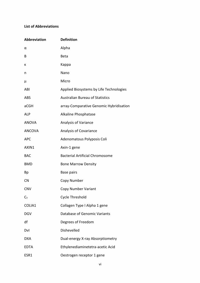
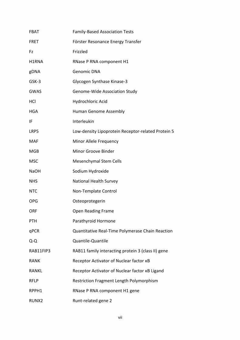
List of Abbreviations

Abbreviation Definition

α Alpha

Β Beta

κ Kappa

n Nano

µ Micro

ABI Applied Biosystems by Life Technologies

ABS Australian Bureau of Statistics

aCGH array-Comparative Genomic Hybridisation

ALP Alkaline Phosphatase

ANOVA Analysis of Variance

ANCOVA Analysis of Covariance

APC Adenomatous Polyposis Coli

AXIN1 Axin-1 gene

BAC Bacterial Artificial Chromosome

BMD Bone Marrow Density

Bp Base pairs

CN Copy Number

CNV Copy Number Variant

CT Cycle Threshold

COLIA1 Collagen Type I Alpha 1 gene

DGV Database of Genomic Variants

df Degrees of Freedom

DvI Dishevelled

DXA Dual-energy X-ray Absorptiometry

EDTA Ethylenediaminetetra-acetic Acid

ESR1 Oestrogen receptor 1 gene

vii

FBAT Family-Based Association Tests

FRET Förster Resonance Energy Transfer

Fz Frizzled

H1RNA RNase P RNA component H1

gDNA Genomic DNA

GSK-3 Glycogen Synthase Kinase-3

GWAS Genome-Wide Association Study

HCl Hydrochloric Acid

HGA Human Genome Assembly

IF Interleukin

LRP5 Low-density Lipoprotein Receptor-related Protein 5

MAF Minor Allele Frequency

MGB Minor Groove Binder

MSC Mesenchymal Stem Cells

NaOH Sodium Hydroxide

NHS National Health Survey

NTC Non-Template Control

OPG Osteoprotegerin

ORF Open Reading Frame

PTH Parathyroid Hormone

qPCR Quantitative Real-Time Polymerase Chain Reaction

Q-Q Quantile-Quantile

RAB11FIP3 RAB11 family interacting protein 3 (class II) gene

RANK Receptor Activator of Nuclear factor κB

RANKL Receptor Activator of Nuclear factor κB Ligand

RFLP Restriction Fragment Length Polymorphism

RPPH1 RNase P RNA component H1 gene

RUNX2 Runt-related gene 2

viii

SCGH Sir Charles Gairdner Hospital

SD Standard Deviation

SNP Single Nucleotide Polymorphism

SOST Sclerostin

SPSS Statistical Package for the Social Sciences

TF Transcription Factor

TGF-β Transforming Growth Factor-Beta

TNF-α Tumour Necrosis Factor-Alpha

Tris Trizma Base

VDR Vitamin D Receptor gene

VNTR Variable Number Tandem Repeat

UCSC University of California Santa Cruz

ix

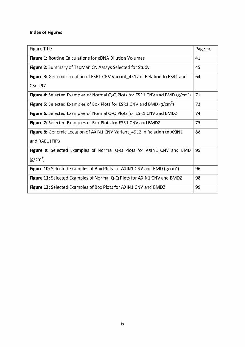
Index of Figures

Figure Title Page no.

Figure 1: Routine Calculations for gDNA Dilution Volumes 41

Figure 2: Summary of TaqMan CN Assays Selected for Study 45

Figure 3: Genomic Location of ESR1 CNV Variant_4512 in Relation to ESR1 and

C6orf97

64

Figure 4: Selected Examples of Normal Q-Q Plots for ESR1 CNV and BMD (g/cm2) 71

Figure 5: Selected Examples of Box Plots for ESR1 CNV and BMD (g/cm2) 72

Figure 6: Selected Examples of Normal Q-Q Plots for ESR1 CNV and BMDZ 74

Figure 7: Selected Examples of Box Plots for ESR1 CNV and BMDZ 75

Figure 8: Genomic Location of AXIN1 CNV Variant_4912 in Relation to AXIN1

and RAB11FIP3

88

Figure 9: Selected Examples of Normal Q-Q Plots for AXIN1 CNV and BMD

(g/cm2)

95

Figure 10: Selected Examples of Box Plots for AXIN1 CNV and BMD (g/cm2) 96

Figure 11: Selected Examples of Normal Q-Q Plots for AXIN1 CNV and BMDZ 98

Figure 12: Selected Examples of Box Plots for AXIN1 CNV and BMDZ 99

x

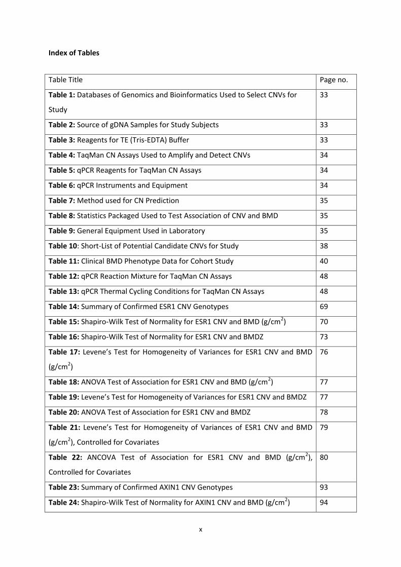
Index of Tables

Table Title Page no.

Table 1: Databases of Genomics and Bioinformatics Used to Select CNVs for

Study

33

Table 2: Source of gDNA Samples for Study Subjects 33

Table 3: Reagents for TE (Tris-EDTA) Buffer 33

Table 4: TaqMan CN Assays Used to Amplify and Detect CNVs 34

Table 5: qPCR Reagents for TaqMan CN Assays 34

Table 6: qPCR Instruments and Equipment 34

Table 7: Method used for CN Prediction 35

Table 8: Statistics Packaged Used to Test Association of CNV and BMD 35

Table 9: General Equipment Used in Laboratory 35

Table 10: Short-List of Potential Candidate CNVs for Study 38

Table 11: Clinical BMD Phenotype Data for Cohort Study 40

Table 12: qPCR Reaction Mixture for TaqMan CN Assays 48

Table 13: qPCR Thermal Cycling Conditions for TaqMan CN Assays 48

Table 14: Summary of Confirmed ESR1 CNV Genotypes 69

Table 15: Shapiro-Wilk Test of Normality for ESR1 CNV and BMD (g/cm2) 70

Table 16: Shapiro-Wilk Test of Normality for ESR1 CNV and BMDZ 73

Table 17: Levene’s Test for Homogeneity of Variances for ESR1 CNV and BMD

(g/cm2)

76

Table 18: ANOVA Test of Association for ESR1 CNV and BMD (g/cm2) 77

Table 19: Levene’s Test for Homogeneity of Variances for ESR1 CNV and BMDZ 77

Table 20: ANOVA Test of Association for ESR1 CNV and BMDZ 78

Table 21: Levene’s Test for Homogeneity of Variances of ESR1 CNV and BMD

(g/cm2), Controlled for Covariates

79

Table 22: ANCOVA Test of Association for ESR1 CNV and BMD (g/cm2),

Controlled for Covariates

80

Table 23: Summary of Confirmed AXIN1 CNV Genotypes 93

Table 24: Shapiro-Wilk Test of Normality for AXIN1 CNV and BMD (g/cm2) 94

xi

Table 25: Shapiro-Wilk Test of Normality for AXIN1 CNV and BMDZ 94

Table 26: Selected Examples of Normal Q-Q Plots for AXIN1 CNV and BMDZ 95

Table 27: Selected Examples of Box Plots for AXIN1 CNV and BMDZ 96

Table 28: Levene’s Test for Homogeneity of Variances for AXIN1 CNV and BMD

(g/cm2)

100

Table 29: Independent-Sample T-Test of Association for AXIN1 CNV and BMD

(g/cm2)

101

Table 30: Levene’s Test for Homogeneity of Variances for AXIN1 CNV and BMDZ 101

Table 31: Independent-Sample T-Test of Association for AXIN1 CNV and BMDZ 102

Table 32: Levene’s Test for Homogeneity of Variances for AXIN1 CNV and BMD

(g/cm2), Controlled for Covariates

103

Table 33: ANCOVA Test of Association for AXIN1 CNV and BMD (g/cm2),


104

xii

Abstract

Copy number variation (CNV) is a relatively novel source of genetic variation, involving the

duplication or deletion of segments of genomic DNA (gDNA) sequence, thereby changing

the original number of DNA copies. It is currently gaining widespread recognition from the

scientific community, and it is anticipated to play a major role in the aetiology of human

diseases. However, the extent of its contribution to phenotypic diversity, in terms of

individual susceptibility to disease, remains to be elucidated. Nonetheless, recent studies

have indicated that common complex disease phenotypes, such as osteoporosis, might be

highly susceptible to CNV.

Osteoporosis is a common and debilitating skeletal condition, imposing significant clinical

and socioeconomic consequences. The disease is characterised by fragile bones that are

susceptible to fracture due to deregulated bone remodelling, where bone loss exceeds bone

formation. Being a common complex disease, osteoporosis risk is largely determined by the

effect of environmental factors on genetic variants. Moreover, identification of the genetic

variants associated with osteoporosis is widely anticipated for the contribution it will make

towards the development of improved measures of disease intervention.

Recent genome-wide association studies (GWASs) have identified that the genes oestrogen

receptor 1 (ESR1) and Axin 1 (AXIN1) potentially play major roles in bone regulation. In

addition, evidence highlights their involvement in key biological processes that regulate

bone turnover. Specifically, ESR1 mediates the response of bone marrow-derived cells to

oestrogen and it has been demonstrated that oestrogen inhibits bone loss, while AXIN1

inhibits Wnt signal transduction and it has been demonstrated that Wnt proteins promote

bone growth. Furthermore, several large-scale analysis projects firmly implicate genetic

xiii

variations of both genes with bone marrow density (BMD), which is the surrogate

phenotype of osteoporosis. Therefore, ESR1 and AXIN1 are both recognised candidates for

the genetic regulation of osteoporosis risk.

This study investigated the potential effect of two novel CNVs of the genes ESR1 and AXIN1,

Variant_4512 and Variant_4912, respectively, in relation to BMD in a population cohort

study of Caucasian women, between the ages of 18 and 83, from Australia and the UK.

Subjects were genotyped for both CNVs, respectively, using real-time quantitative PCR

(qPCR) combined with TaqMan chemistry, and the copy number (CN) quantitation software,

CopyCaller. Subjects were then examined for evidence of association between both CNVs

and three different BMD phenotypes, 1) raw measurement (g/cm2), 2) age-adjusted Z-score,

and 3) controlled for several covariates, at three common skeletal locations of osteoporotic

fracture, 1) lumbar spine, 2) total hip, and 3) femoral neck.

This study confirmed the presence of ESR1 CNV and AXIN1 CNV in the analysed subject

cohort, as indicated by the observation of three distinct CNV genotypes for each,

representing CN loss (CN1) and CN gain (CN3) from the expected wild-type CN in the human

diploid genome (CN2). This study found no evidence of association between both CNVs and

BMD (p = > 0.05) in the analysed subject cohort. Therefore, the hypothesis tested in this

study, that CNV is associated with BMD, was not supported. As a result, it would appear that

the ESR1 CNV Variant_4512 and the AXIN1 CNV Variant_4912 are unlikely to play a major

role in the pathogenesis of osteoporosis in Caucasian women. However, replication studies

and further research would be required to accurately validate this, since this study was

subject to numerous limitations which may have influenced the findings, such as low

statistical power, technical difficulties, limiting experimental reagents, and time constraints.

xiv

In addition, there is evidence from previous studies implicating intron 1 and the 5’ end of

ESR1 and intron 2 of AXIN1 with BMD. Variant_4512 and Variant_4912 encompass the 5’

end of their respective genes, thereby implicating the promoter sequence and regulatory

elements, which in turn implicates the control of gene expression. Therefore, despite the

lack of statistically significant findings in this study, the ESR1 CNV Variant_4512 and the

AXIN1 CNV Variant_4912 both still remain as promising candidates for involvement in BMD

and the risk of osteoporosis. Moreover, other CNVs in the same genomic regions may also

be relevant for future research.

Further research would benefit from addressing the potential effect of environmental risk

factors on CNV. It is possible that the ESR1 CNV Variant_4512 may be modified in an

environment-specific manner, which influences its effect on BMD, as indicated by the

almost statistically significant association between ESR1 CNV and BMD observed in this

study when controlled for covariates at the femoral neck (p = 0.052). Moreover, previous

studies highlight that the majority of known genes subject to CNV are not even located

within the identified region of genomic variation, and also that osteoporosis may be more

susceptible to genetic variation affecting the CN of non-coding regions. Therefore, further

research should also focus on gene expression studies to determine whether the ESR1 CNV

Variant_4512 exerts position effects on the transcriptional control of another gene, which

may in turn be the primary gene associated with osteoporosis.

1

Chapter 1: Introduction

2

1.1 The Impact of Osteoporosis

Osteoporosis is a serious form of musculoskeletal disease [1] and it is the most prevalent

metabolic bone disorder [2]. It is currently estimated to affect over 200 million people

worldwide [3], with postmenopausal women and the elderly of Caucasian descent among

those at the highest risk [4]. The disease is characterised by a gradual, systemic reduction in

the density and structural quality of bones [5], resulting in weakened, fragile bones that are

easily susceptible to fracture [6]. Osteoporotic fractures can occur from minimal trauma,

such as bending, lifting, or even coughing [7], but their incidence is mainly determined by

the frequency and direction of falls [5]. Accordingly, the most common skeletal sites for

osteoporotic fracture are usually where the most impact of a fall is endured, such as the

lumbar spine, hip, pelvis, distal forearm and wrist [4].

Based on the 2007-08 National Health Survey (NHS) conducted by the Australian Bureau of

Statistics (ABS), 620,000 Australians (3.2% of the total population) have doctor-diagnosed

osteoporosis and it occurs mainly in people aged 55 years and over (84.0%), with women

accounting for more than eight out of ten cases (81.9%) [4]. The high incidence of the

disease among women and the elderly may be consistent with trends reported worldwide,

but the prevalence of doctor-diagnosed osteoporosis is most certainly underestimated [4].

The disease lacks overt symptoms and most cases are, therefore, likely to go undiagnosed

[4]. People with osteoporosis are usually unaware that they even have the disease until a

minor trauma results in a fracture and subsequent radiographs demonstrate the

characteristic low bone mass and poor bone quality of osteoporosis [8]. According to the

Osteoporosis Australia research group, a more accurate estimate of the actual number of

people in Australia with the disease is 2.2 million (9% of the total population) [9]. The group

3

also estimates that an osteoporotic fracture occurs every 5-6 minutes in Australia and their

incidence is predicted to rise to every 3-4 minutes by 2021 [9].

Osteoporosis is aptly referred to as ‘the silent disease’ [10], considering that it fails to

demonstrate overt physiological effects until it ultimately manifests itself as a fracture [8].

Osteoporotic fractures are a source of severe pain, immobility and disability [10]. They

cause gradual physical alterations, including loss of height and changes in posture [11], such

as the development of a stooped back (i.e. Dowager’s hump) [9]. Moreover, they can have

psychological effects, such as depression due to chronic pain or loss of independence [11].

Furthermore, clinical research highlights an increased risk of premature mortality with the

disease, which is related to possible co-morbidities such as rheumatism and stroke [12].

Therefore, the quality of life for people affected by osteoporosis is expected to become

progressively worse as the number and severity of fractures increases. It is estimated that

50% of people with one fracture due to osteoporosis will have another. Therefore, the risk

of future fractures increases exponentially with each new fracture. This trend is aptly

referred to as the ‘fracture cascade effect’ [9]. According to Osteoporosis Australia, people

who have had two or more osteoporotic fractures are up to 9 times more likely to have

another fracture, rising to an 11 times greater risk for people who have had three or more

fractures, compared to someone who has not had one [9].

The ‘fracture cascade effect’ constitutes a major socioeconomic concern that will place a

substantial burden on health services as the population ages and the number of

osteoporotic fractures increases [9]. Based on statistical evidence compiled for Australia in

2007 by the Access Economics consultancy group, osteoporosis has a total health

expenditure that exceeds $7 billion per year, with $1.9 billion spent on direct costs, such as

4

pharmaceutical medications and surgical procedures, and a further $5.6 billion spent on

indirect costs, such as financial assistance for lost employment and earnings [13]. These

figures are comparable with the prevalence and expenditure of osteoporosis worldwide

[13]. Therefore, the impact of osteoporosis on sufferers, coupled with the socioeconomic

burden of the disease, deserves attention. The value of disease intervention, in the form of

prevention, diagnosis and treatment, highlights the importance of current research efforts

to better comprehend the pathogenesis of osteoporosis and how it deviates from normal

bone biology.

5

1.2 The Osteoporotic Disease Process

As previously stated, osteoporosis is a systemic bone disease, characterised by increased

fragility of bones, lacking overt symptoms until it clinically manifests itself in the form of

fracture. The three main pathological mechanisms by which skeletal fragility can develop

are as follows; firstly, failure to produce a skeleton of optimal mass and strength during

growth; secondly, excessive bone loss, resulting in decreased bone mass and structural

deterioration of bone tissue micro-architecture; and thirdly, an inadequate bone formation

response [5]. The interplay between these three mechanisms is what ultimately underlies

the development of fragile bones in the osteoporotic disease process [5]. Although the

relative contribution of each remains unclear [5], clinical studies demonstrate that the

underlying cause of these three mechanisms, and hence the potential underlying cause of

osteoporosis, is an imbalance in the bone remodelling process at the cellular level [5],

where bone resorption by osteoclasts exceeds bone formation by osteoblasts [6].

1.2.1 Bone Biology

1.2.1.1 Bone Remodelling

Bone remodelling is a normal, lifelong process by which mature bone tissue is resorbed, or

removed from the skeleton, and new bone tissue is deposited [6]. The skeletal system is

constantly subject to turnover throughout life, with up to 10% of existing bone in a healthy

human skeleton replaced every year [6]. In brief, bone is formed from a combination of

dense compact bone and cancellous bone that is re-enforced at specific points of stress [14].

It is also comprised of blood and lymphatic vessels, nerve fibres, collagen and cells [14].

Furthermore, there are three main cell types found in bone, which are crucial in the bone

6

remodelling process; osteoclasts (resorb bone), osteoblasts (form bone) and osteocytes

(differentiated osteoblasts that mediate the activity of osteoclasts and osteoblasts) [6].

Bone is a dynamic connective tissue, which is highly specialised for its numerous

physiological functions, including protection, support, mechanical load-bearing and the

maintenance of mineral homeostasis and haematopoiesis [15]. Therefore, maintaining

healthy bone tissue is essential for regulating normal physiological activity. The most

dynamic function of bone lies with its capacity to remodel itself in response to metabolic

and structural demands, which is fundamental for maintenance of skeletal integrity and

healthy ageing [16].

The three main purposes of bone remodelling are as follows; firstly, it repairs

microfractures, or perforations in bone tissue that occur during normal daily activity [17];

secondly, it allows the skeletal system to act as a reservoir for minerals that are vital to

physiological processes such as conduction of nerve impulses and muscle contraction [17];

and thirdly, it regulates bone mass at the cellular level [17]. Furthermore, the activities of

bone remodelling’s two sub-processes, bone resorption by osteoclasts and bone formation

by osteoblasts, are tightly coupled, and bone mass will remain stable as long as the amount

of bone removed is evenly balanced by the amount of new bone deposited [16].

1.2.1.2 Bone Regulation

There are several known molecular regulators that determine the rate of bone turnover.

Firstly, it is well documented that circulating hormones control the balance of bone

remodelling [5]. For example, increased levels of oestrogen, calcium, and vitamin D, and

decreased levels of PTH, not only increase the deposition of new bone, but also decrease

bone resorption [5]. Secondly, bone resorption is primarily regulated by the

7

RANK/RANKL/OPG pathway, which plays a central role in osteoclast differentiation and

function [18; 19]. The receptor activator of nuclear factor κB ligand (RANKL) is a molecular

signal produced by osteoblasts and other cell types such as lymphocytes [18]. RANKL binds

to and activates RANK, which is expressed on cells of the osteoclast lineage, thereby

activating osteoclasts and promoting bone resorption [18]. The activity of RANKL is

regulated by the protein osteoprotegerin (OPG), which competes with RANK for binding to

RANKL, and hence suppresses its ability to increase bone resorption [18; 19]. Thirdly, the

Wnt signalling pathway is a recognised, albeit less understood, regulator of bone formation

[19]. Members of the Wnt family of proteins bind to and activate the lipoprotein receptor-

related protein 5 encoded by the gene LRP5 [19]. There are at least 19 Wnt family members,

and it remains to be determined which are the most important in regulating bone

metabolism, but current evidence suggests that Wnt7b and Wnt10b are both involved [19].

A variety of inhibitors of Wnt signalling have also been identified, including soluble frizzled-

related (Fz) proteins and sclerostin (SOST), and it is likely that regulation of bone formation

depends on the balance between levels of stimulatory Wnt molecules and these inhibitors

[19].

Therefore, the key regulators of bone remodelling constitute a finely-tuned process which

relies on complex interactions among multifaceted signalling pathways and multiple local

and systemic regulators of bone cell function to ultimately achieve proper rates of growth,

differentiation and turnover. Moreover, clinical studies have demonstrated how the

disruption of key bone regulators can uncouple the activity between osteoclasts and

osteoblasts and lead to aberrant changes in bone mass. For example, overproduction of

RANKL has been implicated in a variety of degenerative bone diseases (i.e. rheumatoid

8

arthritis) [20] and Wnt signalling pathway mutations have been associated with

osteoporosis [19]. In view of this, when an imbalance in bone remodelling is biased towards

bone resorption, bone tissue is expected to lose minerals much faster than the body can

replace them, resulting in the reduced bone mineral density (BMD) that is characteristic of

osteoporosis.

1.2.2 Primary Risk Factors for Osteoporosis

Osteoporosis may be most prevalent among elderly women of Caucasian descent, but the

disease has the capacity to affect both women and men from all ethnic groups [4], provided

that they are susceptible to specific risk factors. Although a combination of risk factors,

including environmental, age-related, hormonal, dietary, medical, and lifestyle factors, have

been implicated with osteoporosis, the relative contribution of each largely depends on the

form and type of the disease [21]. Osteoporosis can be broadly categorised as either

primary or secondary. Primary osteoporosis is due to ageing, so it mainly affects the elderly

[22], while secondary osteoporosis develops as a consequence of physiological and

pathological effects on the skeleton, resulting from disorders of other organs and tissues,

which can affect people of any age [23]. Primary osteoporosis is the most common form of

the disease and can be further divided into two distinct types based on the pathology

observed [22]. Type I or postmenopausal osteoporosis is associated with the decrease in

oestrogen levels experienced during menopause [5]. Oestrogen is essential for healthy bone

regulation and primarily acts by preventing the activation of enzymes that initiate apoptosis

of bone-forming osteoblasts [5]. In view of this, any event associated with oestrogen

deficiency is expected to be a primary risk factor for osteoporosis in women, such as the

surgical removal of ovaries and anorexia nervosa [24]. Type II or senile osteoporosis is

9

prevalent in women and men, usually aged 70 years and over [23]. Age-related bone loss is

far more complex and multifaceted compared to postmenopausal bone loss and involves a

combination of multiple pathological factors that are already associated with old age, such

as hormonal alterations and cellular changes [25]. The most obvious consequence of age-

related bone loss is the increased risk of fracture due to the frailty and propensity for falls

associated with old age. Therefore, the primary risk factors for developing osteoporosis (i.e.

being a postmenopausal Caucasian woman over 55 years of age) are stable and

unpreventable. However, there are a number of contributing risk factors which can in fact

be modified early in life to dramatically reduce the likelihood of developing the disease [26].

Therefore, the value of early intervention underscores the importance of current research

effort to better detect and treat risk factors contributing to osteoporosis.

10

1.3 Early Intervention of Osteoporosis

1.3.1 Detection of Fracture Risk via BMD

As previously stated, osteoporosis is ‘the silent disease’, which lacks overt physiological

symptoms until a fracture occurs and subsequent radiographs demonstrate the reduced

bone mass and quality, which are characteristic of the disease. Therefore, the clinical and

sociological impact of osteoporosis ultimately lies with the incidence of fractures [19].

Fracture risk has been shown to increase exponentially with a decrease in BMD [22]. As

previously stated, BMD is the most importance consequence of the biased bone remodelling

process underlying osteoporosis. In view of this, low BMD is currently the best predictor of

fracture risk; and accordingly, BMD is typically used as a surrogate phenotype for fracture

risk and bone strength, and hence for osteoporosis itself [28]. BMD is a quantitative trait,

which can be measured on a continuous scale [29], thereby underscoring the genetic

contribution to osteoporosis.

The measurement of BMD can be used to accurately diagnose low BMD before a fracture

even occurs, therefore predicting the risk of future fractures [30]. A BMD test essentially

determines how rich bones are in minerals such as calcium and phosphorus [9]. The higher

the mineral content, the denser and stronger the bones are, and the less likely they are to

fracture easily [9]. There are several different types of BMD tests, which can measure BMD

at various skeletal sites, but usually focus on the bones most likely to fracture due to

osteoporosis (i.e. the posterior-anterior lumbar spine and the proximal femur) [31].

Currently, the standard BMD measurement technology is Dual energy X-ray Absorptiometry

(DXA), because it is the most accurate and uses the least amount of radiation [31]. In brief,

11

DXA is based on the detection of uneven soft tissue composition by the emission of photons

at two different energies [30].

The BMD test is then interpreted by using the BMD measurement (expressed in g/cm2) to

generate a personalised T-score and Z-score. A BMD T-score indicates how dense the bone

is compared to what would be expected in a young healthy adult of the same gender as the

subject [32]. The T-score is the number of standard deviations that the BMD is either above

or below the young average population mean [32]. The more negative the BMD T-score, the

thinner the bones are and thus the more likely they are to fracture easily [32]. Furthermore,

a T-score above -1 is considered normal; between -1 and 2.5 is considered osteopenia (low

bone mass); and, -2.5 or a more negative score is clinically defined as osteoporosis [32].

A BMD Z-score indicates how dense the bone is compared to what would be expected in a

healthy adult of the same age, gender and ethnicity as the subject [32]. The Z-score is the

number of standard deviations that the BMD is either above or below the average

population mean [32]. Ideally, a BMD Z-score should be between -2 and +2 [32]. A BMD Z-

score more negative than -2.5 indicates that bone loss is lower than what would be

expected for someone of the same age [32]. Therefore, it indicates that bone loss is

occurring for a reason unrelated to age, so further investigation would be required.

1.3.2 Prevention of Osteoporosis

As previously stated, the primary risk factors for osteoporosis (i.e. age, gender, and

ethnicity) may be unpreventable, but the contributing factors (i.e. low BMD and high

fracture risk) can be modified early in life to dramatically reduce the likelihood of developing

the disease [26]. Existing measures to prevent osteoporosis focus primarily on building up

12

bone mass, as the more bone mass a person has at the age of peak bone mass, the more

that can be lost without risk of osteoporosis [33]. Moreover, bone mass can be built up

easily through healthy dietary and lifestyle habits between the ages of 25 and 40 [34]. For

example, an adequate intake of calcium and vitamin D [35], along with regular moderate

exercise to improve weight-bearing and strength [36], are known to be important for

preventing osteoporosis.

There are also prevention measures available for people who have already been diagnosed

with osteoporosis, which aim to limit the severity and progression of the disease [37]. There

are a number of drugs available for the prevention of bone resorption. For example,

bisphosphonates possess anti-osteoclastic activity [38]. It must be emphasized that drug

treatments cannot cure osteoporosis; they aim to reduce further bone loss and fracture risk

[4], but must be taken regularly and correctly to maintain their effects [10], which in some

cases may be minimal. Clinical studies have demonstrated that drug treatments reduce

fracture risk by 60%, at most [39]. Therefore, the value of more effective intervention

measures highlights the importance of current research efforts to elucidate the molecular

markers of osteoporosis.

13

1.4 The Genetic Contribution to Osteoporosis

As previously stated, there are many environmental factors, of modifiable sources (i.e. diet,

physical activity, and drug use) and non-modifiable sources (i.e. age, gender, and ethnicity),

which can influence the risk of osteoporosis. However, studies have shown that one of the

most important clinical risk factors for phenotypes related to osteoporosis (i.e. BMD, bone

mass and fracture risk) is a positive family history [19; 40], thereby underscoring the role of

genetics in the aetiology of the disease.

1.4.1 Common Complex Pattern of Inheritance

Like obesity, diabetes, and neurological disorders, osteoporosis is a classic example of a

common, yet complex disease [41]. These diseases involve complex interactions among

multiple risk factors of both genetic and environmental sources [42]. Although the relative

contributions of both sources remain to be fully resolved, studies have indicated that

multiple genetic variants are involved, with each having only a modest effect on common

complex disease risk [43]. This is aptly referred to as the common disease/common variant

hypothesis, which proposes that common disease-causing genetic variants exist in all human

populations and each has a small, additive effect on the overall disease phenotype [44].

Although they may be similar to common monogenic/Mendelian conditions in that they

strongly cluster in families and are highly heritable [43], the underlying genetic contribution

of common complex conditions is inherently different. They do not demonstrate a simple

pattern of inheritance according to Mendel’s Laws [45]. Instead, genetic factors represent

only part of the associated common complex disease risk [46]. Although a person can

harbour a genetic risk factor associated with a particular common complex disease, this

does not necessarily indicate that they are destined to develop the disease [46].

14

Furthermore, the actual common complex disease phenotype largely depends on the

interplay between both genetic and environmental risk factors [47].

In view of this, the genetic contribution to osteoporosis can be easily explained by a

common, yet complex pattern of inheritance, considering that environmental factors have a

strong influence on the risk of disease [48]. Postmenopausal osteoporosis is a perfect

example of how genetic factors can be modified in an environment-specific way to influence

disease risk. Through interaction with oestrogen, the normal expression of the oestrogen

receptor 1 gene (ESR1) promotes healthy bone turnover [19]. Therefore, the activity of ESR1

can be modified by altered levels of oestrogen. For example, a decline in oestrogen levels is

expected to imbalance the regulation of bone turnover, thereby increasing the susceptibility

to phenotypes related to osteoporosis, such as low BMD. Consistent with this, an increase in

oestrogen levels through hormone replacement therapy has been shown to decrease the

risk of osteoporosis [49]. Therefore, rather than identifying the genetic and environmental

components of osteoporosis separately, researchers tend to assess how they interact with

one another [47]. This facilitates the detection of genetic factors that can be modified in an

environment-specific way [46], which may in turn highlight effective targets for therapeutic

intervention.

1.4.2 Identification of Genetic Factors that are Associated with Disease

There are a number of key mechanisms used for the study of osteoporosis. Until recently,

the main strategies that were employed for the detection of common genetic variants and

their association to complex diseases were positional cloning through genome-wide linkage

scans [43] and candidate gene studies [50], respectively. Only a small number of disease

genes have been recognised through these approaches, given their poor statistical power

15

and unreliable reproducibility [43]. Nonetheless, there have been successes in identifying

candidate genes associated with the risk of osteoporosis, that continue to be implicated in

the regulation of bone phenotypes (i.e. bone turnover, bone mass, BMD, and fracture risk)

and include reproductive hormones, calcitrophic hormones, collagen genes, growth factors,

and cytokines, and their corresponding receptors [51].

Association analyses generally require sophisticated statistical designs incorporating all

genetic and non-genetic variations, their interactions and familial corrections [52]. The

recent acceleration in the pace of identifying and validating common genetic variants that

enhance individual susceptibility to complex diseases can be attributed to the advent of

high-throughput, large-scale genome-wide association studies (GWASs), which can identify

disease-associated genes, even when there is no prior biological support for their role in

that particular disease [53]. A GWAS can accurately determine the frequency of a genetic

variant in a case-control study by scanning the entire genome of a person known to be

affected and then comparing the data to the genome of an unaffected person [54].

Furthermore, it is through such analyses that insights into the pathological processes that

influence individual susceptibility to disease can be gained [55]. Accordingly, GWASs have

had successes in identifying hundreds of loci relevant to a range of common complex

diseases and related phenotypes [56]. Although most studies have only been able to

account for, at most, 10% of the phenotypic variance among people [19], this is somewhat

expected of a common complex disease phenotype. As previously stated, the phenotype

depends on multiple genetic variants, with each having only a small additive effect overall,

and their multifaceted interplay with environmental factors.

16

1.4.3 Evidence Supporting the Heritability of Osteoporosis

There are several lines of evidence supporting the contribution of genetic factors towards

phenotypes related to osteoporosis. Twin and family studies have shown that between 50

and 85% of the variance in peak BMD among people is genetically determined [19]. This

finding highlights the potentially strong heritability underlying osteoporosis, considering

that BMD is the best known predictor of the disease [28]. Studies have shown that the

heritability of BMD is usually highest at the most common fracture sites, such as the spine

and hip [19]. In addition to BMD, heritability studies have also shown evidence of a strong

genetic contribution to other determinants of fracture risk, such as BMI, muscle strength,

quantitative ultra-sound properties of bone, femoral neck geometry, and biochemical

markers of bone turnover [19]. For example, a study of biochemical markers that was

conducted by Hunter et al in 2001 reported that the heritability of circulating levels of

vitamin D and PTH was 60 and 65%, respectively [19].

Although the key determinants of fracture risk have shown a strong genetic contribution,

the heritability of fracture on its own has proved more difficult to demonstrate [57].

Conflicting results have been reported, but most studies have estimated the heritability of

fracture to be less than 50% [57]. This may be due to the complexity of the phenotype

considering the multiple risk factors, of both skeletal and non-skeletal sources, and the

associated difficulty in collecting sufficiently powered data sets [19]. However, divergent

results and weak heritability estimations are most likely explained by the fact that the

heritability of fracture has been shown to decrease with age as environmental factors

become more important [19], such as impaired cognition and neuromuscular control, which

can influence the propensity to fall.

17

There is promising evidence for a genetic contribution to bone characteristics relevant to

osteoporosis. However, the underlying genetic basis of the disease, and the extent of this

contribution relative to other risk factors, remains to be fully resolved. Therefore, continued

research efforts are aimed at elucidating the genetic variations that determine individual

susceptibility to osteoporosis.

18

1.5 Human Genetic Variation

As previously stated, osteoporosis is a classic example of a common, yet complex disease,

where the underlying genetic contribution depends on multiple genetic variations, which

each have a small additive effect on the overall phenotype. The advent of high-throughput

sequencing technologies has made it possible for researchers to generate a near-complete

landscape of the human genome [58]. Moreover, recent achievements in biomedical

research, such as the Human Genome Project [58], the International HapMap Project [59],

and continuing advancements in genomics, bioinformatics, research methodologies and

high-throughput sequencing technologies [60], have revealed the abundance of variability

that actually exists within the human genome sequence [58].

Human genetic variation refers to differences, not just among cell types within a person

[61], but also between people [58]. Although humans have been reported to share

approximately 99.9% of their genome sequence [62], evidence suggests that no two

individuals are completely identical, and even monozygotic twins who develop from one

zygote have demonstrated infrequent genetic differences [63]. Numerous studies have

provided examples of evolutionary processes, such as selection, adaptation and genetic drift

as contributing to human genetic variation; however, the relative importance of each

remains unclear [64]. Genetic differences have traditionally been thought to arise during

intrauterine development [63] as a consequence of various mutational events in DNA

replication and meiosis [65]. However, it has been proposed that the mutation rate at most

genomic positions is relatively low compared to that of the most recent ancestor of any two

people [65]. Therefore, although they can arise from de novo mutations, it is reasonable to

assume that the vast majority of genetic differences may be inherited [65]. In view of this,

19

genetic variation is a powerful resource for current research efforts towards elucidating how

the inherited genetic makeup of an individual can influence the variable expression of

particular traits; or put simply, how genotype affects phenotype. Through the analysis of

variable genomic regions, important insights have been gained into the pathological

processes which influence individual susceptibility to disease [55].

1.5.1 Functional Consequence of Human Genetic Variation

Understanding how a DNA sequence exerts a functional effect is crucial towards elucidating

phenotypic diversity [66]. Gene expression represents the most fundamental level at which

the genotype gives rise to the phenotype [67] and virtually all aspects of cellular function

rely on it being properly regulated [68]. Studies have validated that gene expression levels

are indeed predictive of phenotypic traits globally, as demonstrated by genome-wide

expression profiling studies, and also on an individual gene basis, as demonstrated by

studies connecting regulatory genetic variation in adaptively important traits [69].

Therefore, the phenotypic effects of genetic variation are most likely brought about by

changes in gene expression levels [55]. Moreover, disruption of the underlying functional

elements that regulate gene expression may largely determine individual susceptibility to

disease [67].

1.5.1.1 Transcriptional Control of Gene Expression

Researchers have had much success in identifying the cellular mechanisms which are

involved in the control of gene expression [70]. It is generally accepted that transcriptional

control is the main level at which the regulation of gene expression takes place [68]. The

simplest model of transcriptional control involves the binding of transcription factors (TFs),

20

in a sequence-specific manner, to TF binding sites located in promoter sequences [70],

which controls the flow of genetic information from DNA to mRNA [68]. Transcriptional

control itself is influenced by a variety of mechanisms [71]. Evidence suggests that the two

major points of transcriptional control are (i) through the modification of the chromatin

structure of the gene locus, and (ii) through the action of TFs; however, their relative

contributions remain unclear [71]. Although they are often described as separate events,

these two processes are inherently linked, with chromatin structure influencing the

accessibility of DNA to TFs, and the binding of TFs to DNA triggering chromatin modifications

[72]. TFs can act alone or in a complex with regulatory elements [73]. For example, through

interaction with the promoter sequence, TFs bound to an enhancer or repressor can

mediate positive or negative control of the rate of transcription, respectively [74].

Furthermore, most regulatory elements are defined as position- and orientation-

independent [74], and thus may be ‘cis’-acting or ‘trans’-acting – that is, they can be

proximal to the promoter of their target gene [71] or distal and thus active over large

genomic distances [73], respectively. The majority of regulatory effects have been described

as ‘cis’ [61], but a number of ‘trans’ effects have also been described [73].

Distal elements communicate regulatory activity over large spans of intervening DNA [73].

The model which is most commonly encountered in the context of long-range interactions is

the ‘looping’ mechanisms, whereby transcription factors bound to regulatory elements

make direct contact with the promoter sequence while the intervening DNA ‘loops out’ [73].

Therefore, it can be expected that interactions between the promoter and its regulatory

elements can be disrupted through mutation or physical dissociation [71] at overlapping,

nearby, or even long-range distances outside the transcription unit [70]. In some cases, the

21

expression level of a gene can be deleteriously affected by an alteration in its chromosomal

environment, while maintaining an intact transcription unit [62]. This is defined as a

‘position effect’, where the disruption of normal transcriptional control is expected [71]. It is

often less recognised that, in addition to the integrity of protein-coding sequences, human

health also critically depends on the spatially, temporally and quantitatively correct

expression of those genes, and disease can equally be caused by the disruption of the

mechanisms which ensure proper gene expression [71]. Moreover, evidence shows that

when the regulatory system of a gene is disrupted, expression can be adversely affected,

and in some cases, can lead to disease [71].

Therefore, understanding how genetic variation can encompass regulatory regions within

the human genome and subsequently exert a functional consequence is crucial towards

elucidating phenotypic diversity.

1.5.2 Characterisation of Human Genetic Variation

Due to growing evidence that human genetic variation may play an important role in

influencing individual susceptibility to common complex diseases, such as osteoporosis,

there have been considerable research efforts to categorise the genetic differences among

people [75]. The near-completeness of the human genome sequence has enabled the

accurate characterisation and assessment of all types of human genetic variation [62].

Differences in the genetic code are usually defined in terms of their frequency and

nucleotide composition [56]. Despite common differences being more readily studied [43],

genetic variation can be either common or rare, denoting the minor allele frequency (MAF)

in a given population [56]. Common genetic variants are synonymous with ‘polymorphisms’

and are therefore defined as having a MAF greater than 1%, while rare genetic variants have

22

a MAF less than 1% [56]. DNA changes can be further divided into two broad classes based

on their nucleotide composition; single nucleotide and structural [56].

1.5.2.1 Single Nucleotide Polymorphisms (SNPs)

SNPs are the most prevalent source of genetic variation, with over 11 million reported to

date [56]. They most often result from a non-repaired error during DNA replication [65]

every 100 to 300 bases along the genome [56], in which one of the four possible nucleotides

is substituted for another [76]. The term ‘polymorphism’ already denotes that they are

common, with an estimated 7 million SNPs occurring in over 5% of a given population, and

the remaining between 1 and 5% [56]. Studies have shown that the vast majority of SNPs

are neutral; that is, they do not contribute to any specific cellular function and achieve

significant frequencies simply by chance [77]. However, depending on their location within

the genome, SNPs can alter sequence-specific cellular processes, such as gene transcription,

transcript processing and protein synthesis [78]. In turn, a proportion of these may be

associated with disease. Therefore, considerable research efforts have been made to

identify SNPs which exert a functional consequence. For example, it has been estimated that

15% of inherited genetic diseases in humans are caused by deleterious mutations that

interfere with mRNA splicing [79]. Given the vast number of SNPs within the human

genome, GWASs are often limited by the overwhelming number of markers to be screened

[56]. However, this problem is usually overcome by prioritising markers of interest according

to sequence-based features that can predict functional relevance [78], including distance

from transcription factor start site, presence of flanking G and C nucleotides and sequence

repetitiveness [80]. There has been much success in identifying and validating thousands of

functional SNPs that are associated with a diverse range of human diseases [56].

23

Until recently, disease association studies focused predominantly on the role of SNPs [81].

The prevailing view had been that they were the most abundant source of genetic variation

among humans [81] and were thus underlying the bulk of phenotypic diversity associated

with disease [43]. As previously stated, it is widely accepted that osteoporosis is largely

determined by genetic factors; however, the overwhelming extent of this contribution

remains to be fully resolved. Moreover, evidence suggests that SNPs may only account for a

small fraction of the overall risk [44]. For example, there are several known genetic markers,

located within the vitamin D receptor (VDR), collagen type I alpha 1 (COLIA1), and ESR1

genes, which have been implicated in association with osteoporosis risk [22]; however, they

only account for an estimated 5% of the total genetic contribution to the disease [82].

Consequently, it has become increasingly apparent that the remaining undiscovered genetic

contribution may be due to other classes of genetic variation [44]. Therefore, over the past

several years, a new source of genetic variation, defined as structural variation, has been

extensively investigated.

1.5.2.2 Structural Variation

Structural variation is a broad term used to describe any type of genetic variation that alters

chromosome structure [83]. It involves structural changes to DNA segments that typically

span over a kilobase to several megabases [66]. Chromosomal rearrangements have long

been shown to impact human health and disease, although until very recently, this impact

was thought to be from rare, large-scale DNA changes, and reserved only for rare genomic

disorders (i.e. Down’s syndrome) [83]. The recent development of array-comparative

genomic hybridisation (aCGH) and other high-throughput genome-scanning technologies

facilitated the detection of smaller and more abundant chromosomal rearrangements [81].

24

Moreover, with the recognition of structural variation in otherwise healthy people [84], it

has been widely anticipated for its contribution to some of the unexplained heritability

underlying common complex diseases, such as osteoporosis [86]. However, the extent of

functional structural variation within the human genome is only just beginning to be

appreciated, and current knowledge appears to be far from complete. For example,

although currently published data may have defined more than 1500 independent sites

representing 100 to 150 megabases of the human genome sequence as being structurally

variable [85], comparison of these datasets shows a relatively small amount of overlap

between studies [86]. Therefore, it is possible that only a fraction of the total amount of

structural genetic variation has been ascertained to date. Structural variation exists in a

variety of forms [66], which are broadly defined as either ‘balanced’ or ‘unbalanced’ [84],

depending on whether the amount of diploid wild-type DNA actually changes [85]. Balanced

variants include inversions, insertions, and translocations [84], which rearrange the

orientation of a DNA segment without actually changing the amount of DNA [87], while

unbalanced variants include deletions and duplications [84], which directly change the

amount of DNA [87]. Like other forms of genetic variation, structural alterations may exert a

deleterious phenotypic consequence [62], presumably owing to changes involving functional

genes. Furthermore, structural genetic variants can cover millions of nucleotides [83] and

are thus likely to comprise of fully functional DNA sequences, which may already be subject

to other forms of genetic variation. Interestingly, rapidly accumulating evidence suggests

that structural genetic variants comprise a large proportion of SNPs [66]. Therefore, they are

likely to make an even greater contribution to phenotypic diversity among humans, such as

individual susceptibility to disease.

25

1.6 Copy Number Variation (CNV)

CNV is the most common source of structural genetic variation [84]. It involves the

duplication or deletion of DNA segments [84], consequently changing the structure of

chromosomes by joining together formally separated DNA sequences [88]. Therefore, CNV is

used to describe any change to the original number of DNA copies [84]. It is still a relatively

new area of genetic research, which is currently gaining widespread recognition from the

scientific community. Therefore, the overwhelming majority of information pertaining to

CNV remains to be fully resolved.

1.6.1 Mechanism of CNV Formation

Researchers have proposed a number of feasible mechanisms which may contribute to the

formation of CNV [85]. Although the precise mechanism of formation is not yet completely

understood, the fact that CNVs have been shown to preferentially occur near or within

segmentally duplicated genomic regions has provided some important clues as to their

origins [89]. Segmental duplications are thought to arise through tandem replication of DNA

sequences, followed by subsequent rearrangements that place the duplicated sequence at

different chromosomal positions [81]. During the metaphase stage of cellular meiosis,

maternal and paternal chromosomes align using sequence homology as a guide to pair and

initiate recombination of homologous pairs of chromosomes [88]. However, the presence of

segmental duplications can ‘trick’ the recombination machinery to initiate a cross-over

event where it normally would not occur, which is aptly described as ‘non-allelic

homologous recombination’ [88]. As a result, deletions or further duplications of the DNA

can occur [88], thereby changing the wild-type number of DNA copies and promoting

variability at a particular locus. Although the precise mechanism of CNV formation remains

26

to be fully elucidated, evidence suggests that CNVs can be either inherited or caused by de

novo mutations which can arise both meiotically and somatically, as indicated by the

observation that DNA CN can vary between identical twins and also between different

organs and tissues within the same person [88].

1.6.2 Functional Consequence of CNV

Despite being a complex phenomenon which remains to be fully understood, there are

several lines of evidence which support the functional significance of CNV. Like other forms

of genetic variation, purifying and adaptive natural selection pressures appear to have

influenced the frequency distributions of selective CNVs [84], indicating that they have at

least some functional significance. Moreover, despite being less abundant than SNPs, CNVs

generally account for far more nucleotide variation [84], which can be attributed to their

sheer size. By encompassing large-scale segments of DNA [55], they are likely to overlap

functional regions of the genome. In part, the functional consequence of CNV appears easily

interpretable, considering how the human diploid genome is sensitive to changes affecting

gene dosage [85]. Possessing the wild-type standard two copies provides a back-up for most

genes should one be lost through mutation [83]. However, for a particular sub-set of genes

known as haplo-insufficient and triplo-abnormal, two copies are essential for viability and if

a copy is gained or lost, respectively, normal function cannot be sustained [83]. Although

the functional consequence of CNV is largely expected to be a result of direct gene dosage

effects, recent evidence indicates that the majority of known genes subject to CNV are not

even located within the identified region of genetic variation [84]. Considering that a large

proportion of the human genome, currently estimated at 12%, is subject to CNV [88], it has

become increasingly recognised that non-coding regions may be as equally relevant as those

27

which code for proteins [90]. Therefore, CNV may also affect genes indirectly through

disruption of the regulatory mechanisms which control their expression [55]. Furthermore,

studies have identified much of the genetic contribution influencing gene expression as

being located proximal to the genes that actually exhibit the variation [91]. This signal is

described as ‘cis’, which indicates that the variant is located within a regulatory sequence

whose target gene is located on the same chromosome [71]. For example, studies have

demonstrated that the disruption of long-range ‘cis’-acting regulatory elements constitute

part of numerous common complex disease loci [91]. Despite the apparent importance of

‘cis’-acting regulators, ‘trans’-acting may equally contribute to genetic expression variation

[73]. Disruption of long-range control is most readily identified when the resultant

phenotype is a loss-of-function change [91], which consequently is the most likely outcome

of CNV [92].

1.6.3 CNVs and Disease

It is clear than CNV plays a significant role in the genetic aetiology of numerous diseases,

with evidence supporting models of both highly-penetrant rare variants [93] and common

CN polymorphisms with small effect sizes [94]. CNVs can be deleterious due to a number of

mechanisms, including formation of new alleles via changes in coding sequence, gain or loss

of alleles via changes in gene dosage, or ‘cis’ and ‘trans’ position effects via changes in gene

regulation [95]. Moreover, studies have observed that many of the functional DNA

sequences encompassed by CNVs are associated with biological mechanisms mediating

immune responsiveness, cellular metabolism, and membrane surface interactions,

otherwise defined as ‘environmental sensor’ genes [84]. Although they are not necessarily

critical for growth or development, these genes facilitate enhanced perception and

28

interaction with the constantly-changing environment [84]. Therefore, in the context of

common complex diseases, such as osteoporosis, this could explain how CNVs can be

present within the genome of an otherwise healthy person and not cause the disease

directly, but instead contribute to enhanced susceptibility (i.e. low BMD, poor structural

quality of bones and fracture risk) given exposure to specific environmental factors (i.e. the

frailty associated with old age and the related propensity to fall).

Rapidly-developing technologies such as aCGH platforms have led to recent successes in the

identification and validation of thousands of heritable CNVs [84]. However, there are a

number of issues that complicate large-scale analyses of the role of CNV in disease. Perhaps

most difficult is actually identifying which CNVs are causal in a given disease. The candidate

gene approach is based on the assumption that if a gene is important for biological reasons,

it may also affect the trait of clinical interest [96]. For example, in the context of

osteoporosis, the genes that are involved in the key biological processes related to the

regulation of bone (i.e. the hormonal endocrine system and the RANK/RANKL/OPG and Wnt

signalling pathways) are expected to influence phenotypes related to osteoporosis risk (i.e.

low BMD, poor structural quality of bones and fracture risk). However, because many

candidate gene studies lack both sufficiently powered data from small sample sizes and

replication groups with which to validate findings [43], the status of many CNVs in disease

remain uncertain [89].

Although establishing a causal relationship between CNV and disease remains challenging

for researchers [89], recent studies have demonstrated that known CNVs account for up to

15% of the total genetic variation in gene expression [55]. Therefore, considering that gene

expression is the most fundamental level at which the genotype gives rise to the phenotype

29

[67], and also that the full extent of CNV within the human genome has not yet been fully

resolved [89]; CNVs may potentially contribute substantially to phenotypic diversity related

to individual susceptibility to disease [69]. Furthermore, CNV may even constitute a

substantial part of the undiscovered genetic contribution towards phenotypes related to the

risk of osteoporosis [82], but further research is required.

30

1.7 Statement of Thesis

1.7.1 General Purpose of Research

Given what is already known about osteoporosis, gene expression, and CNV, the general

purpose of this study is to investigate whether CNV of genomic regions, whose wild-type

expression has previously been implicated with the regulation of bone, has an influence on

the regulation of the surrogate phenotype for osteoporosis, BMD, and thus whether it

influences the risk of developing the disease.

1.7.2 Hypothesis

Therefore, the hypothesis to be tested in this study is that CNV is associated with BMD.

1.7.3 Aims of Study

To address the hypothesis of this study, and to better elucidate the potential relationship

between CNV and osteoporosis for further research, the main aim of this study is to

examine the potential effect of two novel CNVs of the genes ESR1 and AXIN1, Variant_4512

and Variant_4912, respectively, in relation to BMD, in a population cohort study of

Caucasian women, between the ages of 18 and 83, from Australia and the UK.

Furthermore, the specific aims of this study, with which the main aim will be addressed, are

as follows:

1) To attempt the accurate detection and quantitation of Variant_4512 and Variant_4912,

respectively, in every subject of the study cohort, using relatively novel CNV genotyping

techniques via qPCR combined with TaqMan chemistries, and the CN quantitation software,

CopyCaller.

31

2) To examine the potential effect of Variant_4512 and Variant_4912, respectively, in the

study cohort, in relation to three different BMD phenotypes; 1) raw measurement (g/cm2),

2) age-adjusted Z-score, and 3) controlled for several covariates, at three common skeletal

locations of osteoporotic fracture; 1) lumbar spine, 2) total hip, and 3) femoral neck, using

analyses of variance via the statistics software, SPSS.

32

Chapter 2: Materials and Methods

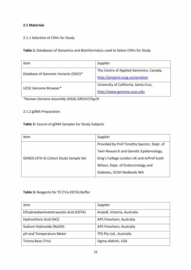
33

2.1 Materials

2.1.1 Selection of CNVs for Study

Table 1: Databases of Genomics and Bioinformatics used to Select CNVs for Study

Item Supplier

Database of Genomic Variants (DGV)* The Centre of Applied Genomics, Canada,

http://projects.tcag.ca/variation

UCSC Genome Browser* University of California, Santa Cruz,

http://www.genome.ucsc.edu

*Human Genome Assembly (HGA) GRCh37/hg19

2.1.2 gDNA Preparation

Table 2: Source of gDNA Samples for Study Subjects

Item Supplier

GENOS (STH-S) Cohort Study Sample Set

Provided by Prof Timothy Spector, Dept. of

Twin Research and Genetic Epidemiology,

King’s College London UK and A/Prof Scott

Wilson, Dept. of Endocrinology and

Diabetes, SCGH Nedlands WA

Table 3: Reagents for TE (Tris-EDTA) Buffer

Item Supplier

Ethylenediaminetetraacetic Acid (EDTA) AnalaR, Victoria, Australia

Hydrochloric Acid (HCl) APS Finechem, Australia

Sodium Hydroxide (NaOH) APS Finechem, Australia

pH and Temperature Meter TPS Pty Ltd., Australia

Trizma Base (Tris) Sigma-Aldrich, USA

http://projects.tcag.ca/variation

http://www.genome.ucsc.edu/

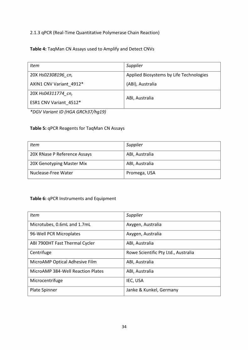
34

2.1.3 qPCR (Real-Time Quantitative Polymerase Chain Reaction)

Table 4: TaqMan CN Assays used to Amplify and Detect CNVs

Item Supplier

20X Hs02308196_cn,

AXIN1 CNV Variant_4912*

Applied Biosystems by Life Technologies

(ABI), Australia

20X Hs04311774_cn,

ESR1 CNV Variant_4512* ABI, Australia

*DGV Variant ID (HGA GRCh37/hg19)

Table 5: qPCR Reagents for TaqMan CN Assays

Item Supplier

20X RNase P Reference Assays ABI, Australia

20X Genotyping Master Mix ABI, Australia

Nuclease-Free Water Promega, USA

Table 6: qPCR Instruments and Equipment

Item Supplier

Microtubes, 0.6mL and 1.7mL Axygen, Australia

96-Well PCR Microplates Axygen, Australia

ABI 7900HT Fast Thermal Cycler ABI, Australia

Centrifuge Rowe Scientific Pty Ltd., Australia

MicroAMP Optical Adhesive Film ABI, Australia

MicroAMP 384-Well Reaction Plates ABI, Australia

Microcentrifuge IEC, USA

Plate Spinner Janke & Kunkel, Germany

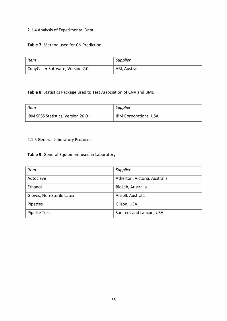
35

2.1.4 Analysis of Experimental Data

Table 7: Method used for CN Prediction

Item Supplier

CopyCaller Software, Version 2.0 ABI, Australia

Table 8: Statistics Package used to Test Association of CNV and BMD

Item Supplier

IBM SPSS Statistics, Version 20.0 IBM Corporations, USA

2.1.5 General Laboratory Protocol

Table 9: General Equipment used in Laboratory

Item Supplier

Autoclave Atherton, Victoria, Australia

Ethanol BioLab, Australia

Gloves, Non-Sterile Latex Ansell, Australia

Pipettes Gilson, USA

Pipette Tips Sarstedt and Labcon, USA

36

2.2 Methods

Notes:

a) This study investigated the potential effect of two different CNVs on BMD, and although

the CNVs were analysed separately, all methods were applied in exactly the same manner,

unless otherwise indicated. Therefore, in this thesis, the analyses of ESR1 CNV and AXIN1

CNV are collectively described in the following general methods section.

b) The dedicated contribution of Shelby Chew with laboratory technical assistance must be

acknowledged.

2.2.1 Selection of CNVs for Study

2.2.1.1 Identification of Potential Osteoporosis Genes

Genes that are potentially relevant to osteoporosis and its related phenotypes, including

those that regulate bone turnover, bone mass, BMD, and fracture risk, were broadly

identified via an extensive interrogation of various scientific papers and review articles.

Focus was eventually directed towards two main resources; a collaborative meta-analysis

implicating 150 candidate genes with osteoporosis and fracture [97], and a meta-analysis of

five GWAS implicating 20 genetic loci in association with BMD [98]. Genomic regions of

interest were short-listed for further investigation based on subjective criteria. Firstly, they

had to have a significant association to a bone trait, such as bone turnover, bone mass,

BMD, or fracture risk, that was reported in a discovery set, and which had been confirmed in

further replication sets. Secondly, they could be mapped to SNPs implicated with bone

traits. As a result, many of the genomic regions of interest selected for this study had

already been firmly implicated with phenotypes related to osteoporosis risk. The genomic

37

regions of interest in this study were short-listed as follows; ARHGAP1, AXIN1, ANAPC1,

C17orf53, C18orf19, DCDC5, EIF4G3, ESR1, FOXL1, GPR177, LRP5L, NTAN1, MEPE, OPG,

RANKL, SOX9, STARD3NL, TNFSF11, and ZBTB40.

2.2.1.2 Identification of CNVs

CNVs that have been detected for the genomic regions of interest were identified via the

DGV. It was initially intended for CNVs to be selected as potential candidates for this study

based on subjective criteria; however, slight modifications had to be made. Firstly, for this

study to have been a true replication study in terms of CNV detection, the discovery cohort

from which the CNV was initially detected should have been representative of the cohort

that would be used in this current study [99]. Therefore, both sets of subjects should have

shared similar distributions of characteristics (i.e. age, gender, and ethnicity). However,

considering that no discovery set was comprised exclusively of Caucasian women between

the ages of 18 and 83 [100], as was used in this current study, this particular point of criteria

could not be fulfilled.

Secondly, a CNV observed in 10% or more of the analysed discovery cohort was estimated

as a common frequency [101], and was thus interpreted as likely to be common in any

similar human population. However, as previously stated, the population in this current

study was not similar to any discovery population. Nonetheless, these CNVs were still

selected for this study because they were interpreted as common variants; and considering

that common variants are expected to constitute the genetic contribution of osteoporosis

(Refer to Section 1.4.1), they appeared extremely relevant for this study. The CNVs of

interest in this study were short-listed as follows;

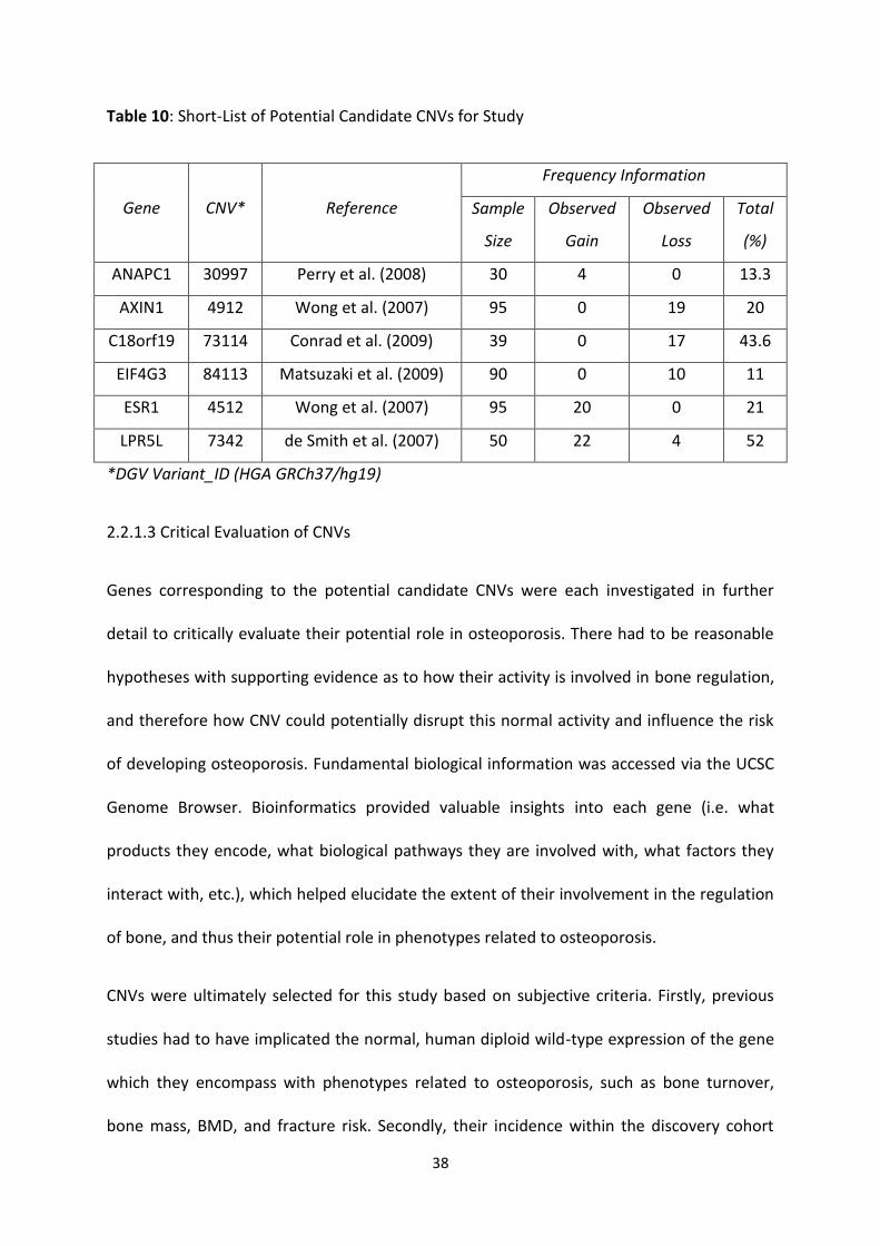
38

Table 10: Short-List of Potential Candidate CNVs for Study

Gene CNV* Reference

Frequency Information

Sample

Size

Observed

Gain

Observed

Loss

Total

(%)

ANAPC1 30997 Perry et al. (2008) 30 4 0 13.3

AXIN1 4912 Wong et al. (2007) 95 0 19 20

C18orf19 73114 Conrad et al. (2009) 39 0 17 43.6

EIF4G3 84113 Matsuzaki et al. (2009) 90 0 10 11

ESR1 4512 Wong et al. (2007) 95 20 0 21

LPR5L 7342 de Smith et al. (2007) 50 22 4 52

*DGV Variant_ID (HGA GRCh37/hg19)

2.2.1.3 Critical Evaluation of CNVs

Genes corresponding to the potential candidate CNVs were each investigated in further

detail to critically evaluate their potential role in osteoporosis. There had to be reasonable

hypotheses with supporting evidence as to how their activity is involved in bone regulation,

and therefore how CNV could potentially disrupt this normal activity and influence the risk

of developing osteoporosis. Fundamental biological information was accessed via the UCSC

Genome Browser. Bioinformatics provided valuable insights into each gene (i.e. what

products they encode, what biological pathways they are involved with, what factors they

interact with, etc.), which helped elucidate the extent of their involvement in the regulation

of bone, and thus their potential role in phenotypes related to osteoporosis.

CNVs were ultimately selected for this study based on subjective criteria. Firstly, previous

studies had to have implicated the normal, human diploid wild-type expression of the gene

which they encompass with phenotypes related to osteoporosis, such as bone turnover,

bone mass, BMD, and fracture risk. Secondly, their incidence within the discovery cohort

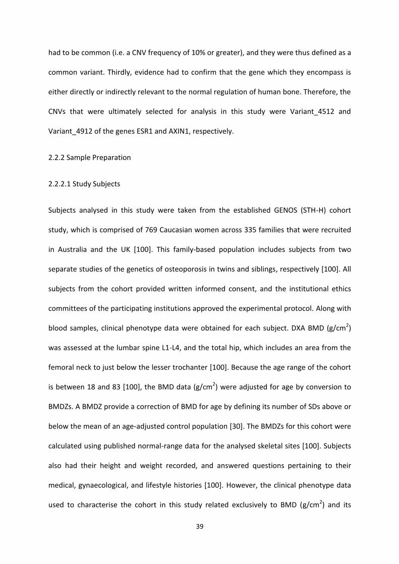
39

had to be common (i.e. a CNV frequency of 10% or greater), and they were thus defined as a

common variant. Thirdly, evidence had to confirm that the gene which they encompass is

either directly or indirectly relevant to the normal regulation of human bone. Therefore, the

CNVs that were ultimately selected for analysis in this study were Variant_4512 and

Variant_4912 of the genes ESR1 and AXIN1, respectively.

2.2.2 Sample Preparation

2.2.2.1 Study Subjects

Subjects analysed in this study were taken from the established GENOS (STH-H) cohort

study, which is comprised of 769 Caucasian women across 335 families that were recruited

in Australia and the UK [100]. This family-based population includes subjects from two

separate studies of the genetics of osteoporosis in twins and siblings, respectively [100]. All

subjects from the cohort provided written informed consent, and the institutional ethics

committees of the participating institutions approved the experimental protocol. Along with

blood samples, clinical phenotype data were obtained for each subject. DXA BMD (g/cm2)

was assessed at the lumbar spine L1-L4, and the total hip, which includes an area from the

femoral neck to just below the lesser trochanter [100]. Because the age range of the cohort

is between 18 and 83 [100], the BMD data (g/cm2) were adjusted for age by conversion to

BMDZs. A BMDZ provide a correction of BMD for age by defining its number of SDs above or

below the mean of an age-adjusted control population [30]. The BMDZs for this cohort were

calculated using published normal-range data for the analysed skeletal sites [100]. Subjects

also had their height and weight recorded, and answered questions pertaining to their

medical, gynaecological, and lifestyle histories [100]. However, the clinical phenotype data

used to characterise the cohort in this study related exclusively to BMD (g/cm2) and its

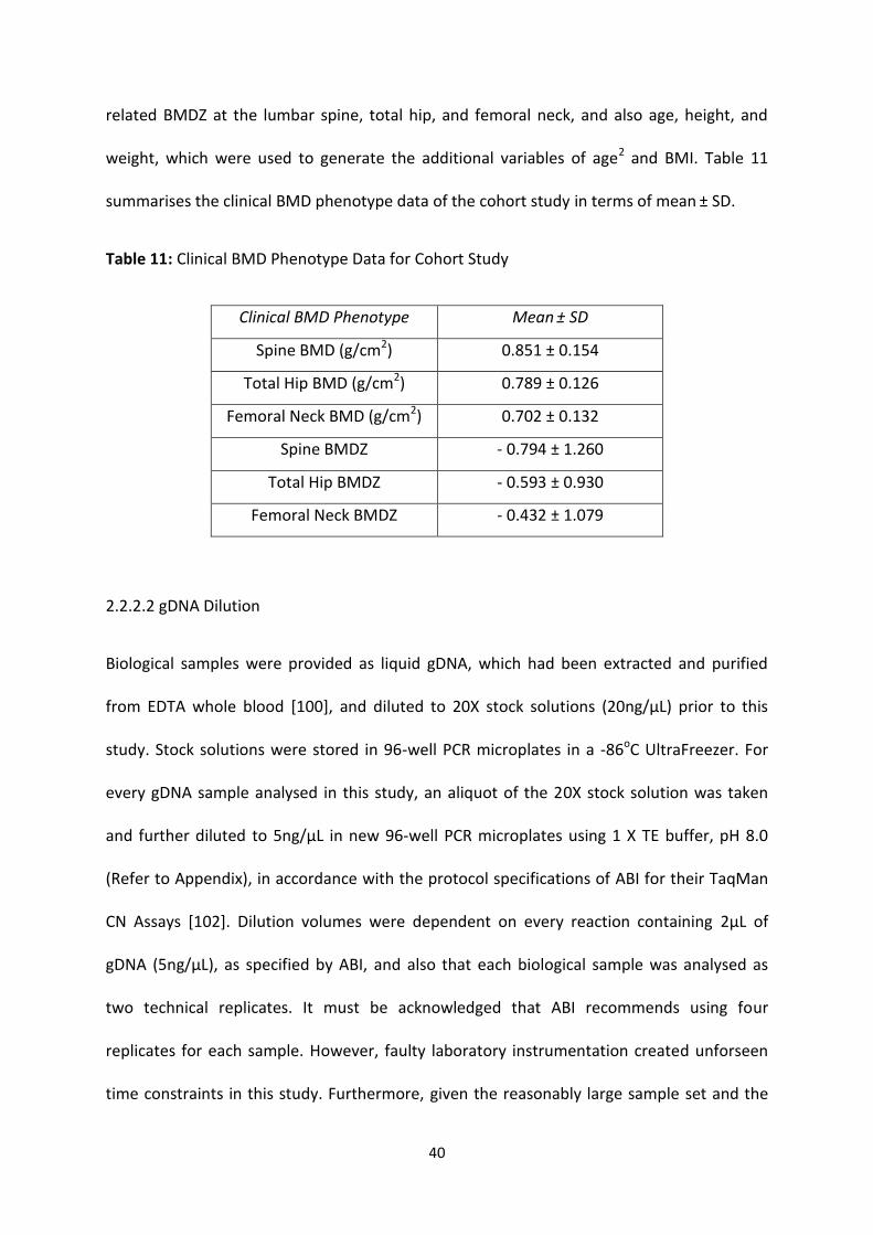
40

related BMDZ at the lumbar spine, total hip, and femoral neck, and also age, height, and

weight, which were used to generate the additional variables of age2 and BMI. Table 11

summarises the clinical BMD phenotype data of the cohort study in terms of mean ± SD.

Table 11: Clinical BMD Phenotype Data for Cohort Study

Clinical BMD Phenotype Mean ± SD

Spine BMD (g/cm2) 0.851 ± 0.154

Total Hip BMD (g/cm2) 0.789 ± 0.126

Femoral Neck BMD (g/cm2) 0.702 ± 0.132

Spine BMDZ - 0.794 ± 1.260

Total Hip BMDZ - 0.593 ± 0.930

Femoral Neck BMDZ - 0.432 ± 1.079

2.2.2.2 gDNA Dilution

Biological samples were provided as liquid gDNA, which had been extracted and purified

from EDTA whole blood [100], and diluted to 20X stock solutions (20ng/µL) prior to this

study. Stock solutions were stored in 96-well PCR microplates in a -86oC UltraFreezer. For

every gDNA sample analysed in this study, an aliquot of the 20X stock solution was taken

and further diluted to 5ng/µL in new 96-well PCR microplates using 1 X TE buffer, pH 8.0

(Refer to Appendix), in accordance with the protocol specifications of ABI for their TaqMan

CN Assays [102]. Dilution volumes were dependent on every reaction containing 2µL of

gDNA (5ng/µL), as specified by ABI, and also that each biological sample was analysed as

two technical replicates. It must be acknowledged that ABI recommends using four

replicates for each sample. However, faulty laboratory instrumentation created unforseen

time constraints in this study. Furthermore, given the reasonably large sample set and the

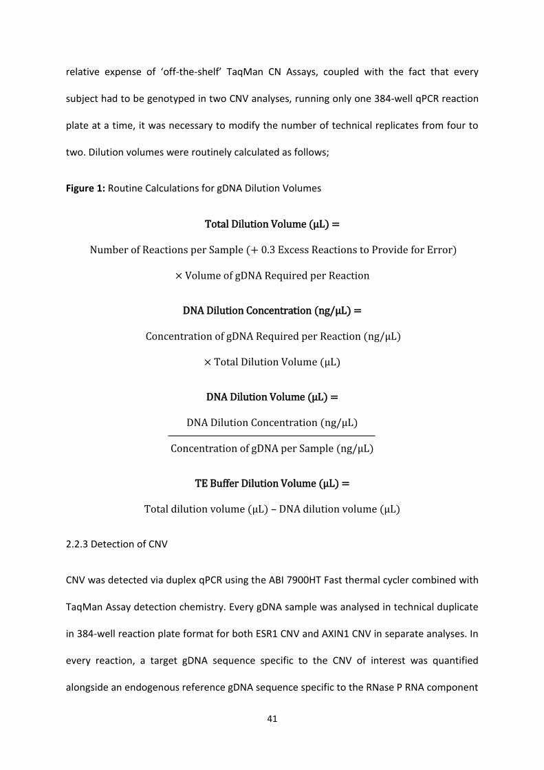
41

relative expense of ‘off-the-shelf’ TaqMan CN Assays, coupled with the fact that every

subject had to be genotyped in two CNV analyses, running only one 384-well qPCR reaction

plate at a time, it was necessary to modify the number of technical replicates from four to

two. Dilution volumes were routinely calculated as follows;

Figure 1: Routine Calculations for gDNA Dilution Volumes

Total Dilution Volume (µL) =

Number of Reactions per Sample (+ 0.3 Excess Reactions to Provide for Error)

× Volume of gDNA Required per Reaction

DNA Dilution Concentration (ng/µL) =

Concentration of gDNA Required per Reaction (ng/µL)

× Total Dilution Volume (µL)

DNA Dilution Volume (µL) =

DNA Dilution Concentration (ng/µL)

Concentration of gDNA per Sample (ng/µL)

TE Buffer Dilution Volume (µL) =

Total dilution volume (µL) – DNA dilution volume (µL)

2.2.3 Detection of CNV

CNV was detected via duplex qPCR using the ABI 7900HT Fast thermal cycler combined with

TaqMan Assay detection chemistry. Every gDNA sample was analysed in technical duplicate

in 384-well reaction plate format for both ESR1 CNV and AXIN1 CNV in separate analyses. In

every reaction, a target gDNA sequence specific to the CNV of interest was quantified

alongside an endogenous reference gDNA sequence specific to the RNase P RNA component

42

H1 (H1RNA) gene (RPPH1), which is known to be present as the wild-type number of copies

(i.e. CN2) in the human diploid genome, and does not display CNV [103]. CNV genotypes

were subsequently determined using the computer software program, CopyCaller, which

performed comparative CT (ΔΔCT) relative quantitation analysis of the qPCR data from the

TaqMan Assay experiments. This method of relative quantitation determined the relative

CN of the target CNV (ESR1 and AXIN1, respectively) in every gDNA sample, normalised to

the known CN2 of the reference gene.

2.2.3.1 Overview of qPCR

qPCR, like a conventional PCR, involves the amplification of specific or complementary DNA

sequences [104]. In a conventional PCR, the amplified product is detected and measured by

‘end-point’ analysis, such as agarose gel electrophoresis or DNA sequencing [104]. In

contrast, qPCR enables the accumulation of amplified product to be detected and measured

as the reaction progresses [104], hence it being referred to as ‘real-time’ analysis. This

function is made possible by a molecule in the reaction that reports an increase in the

amount of DNA amplicon with a proportional increase in fluorescent signal [104]. Moreover,

specialised thermal cyclers, which are equipped with fluorescence detection modules,

monitor and measure the fluorescence as amplification progresses [105]. During each

amplification cycle, the amount of template DNA increases exponentially (i.e. doubles in

amount), but as the reagents become used up, the reaction slows and enters a plateau

phase [106]. The level of fluorescent initially cannot be detected from that of the

background fluorescence [106]. However, enough DNA amplicon is eventually produced to

yield a detectable signal. The amplification cycle in which this occurs is the cycle threshold

(CT) [106]. Considering that the CT is measured during the exponential phase, when the

43

reagents are not limiting, qPCR can accurately calculate the amount of DNA that was initially

present in the reaction [106]. In view of this, if a large amount of DNA is present at the start

of the reaction, fewer amplification cycles will be required for the fluorescence to rise above

background levels and hence the CT value will be low [107]. Conversely, if a small amount of

DNA is present, more amplification cycles will be required for the fluorescence to rise above

background levels and hence the CT value will be high [107].

There are many advantages for using ‘real-time’ chemistries over traditional, ‘end-point’

PCR methods. Firstly, qPCR provides both qualitative and quantitative information with

increased precision, accuracy, and resolution, over a wide dynamic range [108]. Secondly,

results can be measured without agarose gel electrophoresis or DNA sequencing [104],

thereby reducing experiment time and increasing laboratory throughput. Thirdly, it is a

closed-tube system which reduces the opportunities for contamination and eliminates the

need for post-amplification processing [109].

2.2.3.2 Overview of TaqMan Assay Detection Chemistry

The qPCR experiments undertaken in this study used TaqMan-based (i.e. hydrolysis-based

[108]) chemistries to detect changes in DNA quantity. At the initial stage of qPCR, when the

gDNA denatures and the set of assay primers anneal to their specific target sequences, an

oligonucleotide probe anneals specifically to its complementary sequence between the

forward and reverse primer binding sites [108; 110; 111]. This oligonucleotide is labelled

with a fluorescent reporter dye at the 5’ end and a quencher dye at the 3’ end [111]. When

the probe is intact, the reporter is in close proximity to the quencher and the fluorescent

signal emitted by the reporter as it is excited by the thermal cycler’s light source via förster

resonance energy transfer (FRET) is low [108; 110; 111]. During amplification, as Taq DNA

44

polymerase extends from the primers, the 5’ exonuclease activity of the enzyme will cleave

the annealed probe, separating the reporter dye from the quencher dye, relieving the

quenching effect and thus increasing the fluorescent signal [108; 110; 111].

The main advantage of TaqMan-based chemistries over other detection chemistries is that

the fluorescent signal is generated only when there is specific hybridisation of the probe to

the target DNA sequence [108]. Another advantage is that TaqMan probes can be labelled

with different, spectrally distinct reporter dyes [110]. Therefore, reactions can be performed

as duplex, rather than singleplex. In a singleplex reaction, each target sequence of interest is

analysed individually in separate reactions [110]. Conversely, a duplex reaction allows for

the amplification of multiple target sequences within a single tube [110]. Therefore, duplex

reactions confer certain advantages over singleplex reactions. Firstly, there is a reduction in

the amount of starting template DNA required [111]. Secondly, there is an increased

laboratory throughput, with an associated reduction in costly reagent wastage [111].

Thirdly, there is a minimisation of sample handling [111], which reduces potential

opportunities for cross-contamination.

2.2.3.3 Selection of TaqMan Assays used in Study

The TaqMan CN Assays used in this study were selected via the ABI website’s TaqMan CNV

Assay search tool. A multitude of pre-designed assays for human CNV were available to

target a range of different locations across the CNVs of interest in this study. The two

TaqMan CN Assays used for the analyses of ESR1 CNV and AXIN1 CNV, respectively, were

ultimately selected based on subjective criteria. Firstly, it had to target a region somewhere

in the middle of the CNV, so as to ensure adequate coverage across the genomic region of

interest in terms of both annealing and amplification specificity. Secondly, it had to target a

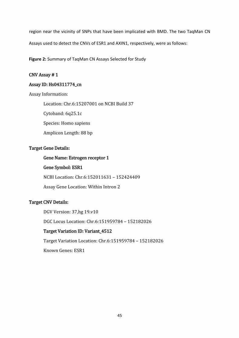
45

region near the vicinity of SNPs that have been implicated with BMD. The two TaqMan CN

Assays used to detect the CNVs of ESR1 and AXIN1, respectively, were as follows:

Figure 2: Summary of TaqMan CN Assays Selected for Study

CNV Assay # 1

Assay ID: Hs04311774_cn

Assay Information:

Location: Chr.6:15207001 on NCBI Build 37

Cytoband: 6q25.1c

Species: Homo sapiens

Amplicon Length: 88 bp

Target Gene Details:

Gene Name: Estrogen receptor 1

Gene Symbol: ESR1

NCBI Location: Chr.6:152011631 – 152424409

Assay Gene Location: Within Intron 2

Target CNV Details:

DGV Version: 37,hg 19.v10

DGC Locus Location: Chr.6:151959784 – 152182026

Target Variation ID: Variant_4512

Target Variation Location: Chr.6:151959784 – 152182026

Known Genes: ESR1

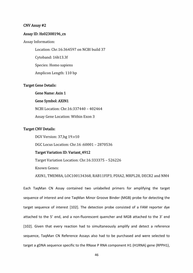
46

CNV Assay #2

Assay ID: Hs02308196_cn

Assay Information:

Location: Chr.16:364597 on NCBI build 37

Cytoband: 16b13.3f

Species: Homo sapiens

Amplicon Length: 110 bp

Target Gene Details:

Gene Name: Axin 1

Gene Symbol: AXIN1

NCBI Location: Chr.16:337440 – 402464

Assay Gene Location: Within Exon 3

Target CNV Details:

DGV Version: 37,hg 19.v10

DGC Locus Location: Chr.16 :60001 – 2870536

Target Variation ID: Variant_4912

Target Variation Location: Chr.16:333375 – 526226

Known Genes:

AXIN1, TMEM8A, LOC100134368, RAB11FIP3, PDIA2, MRPL28, DECR2 and NM4

Each TaqMan CN Assay contained two unlabelled primers for amplifying the target

sequence of interest and one TaqMan Minor Groove Binder (MGB) probe for detecting the

target sequence of interest [102]. The detection probe consisted of a FAM reporter dye

attached to the 5’ end, and a non-fluorescent quencher and MGB attached to the 3’ end

[102]. Given that every reaction had to simultaneously amplify and detect a reference

sequence, TaqMan CN Reference Assays also had to be purchased and were selected to

target a gDNA sequence specific to the RNase P RNA component H1 (H1RNA) gene (RPPH1),

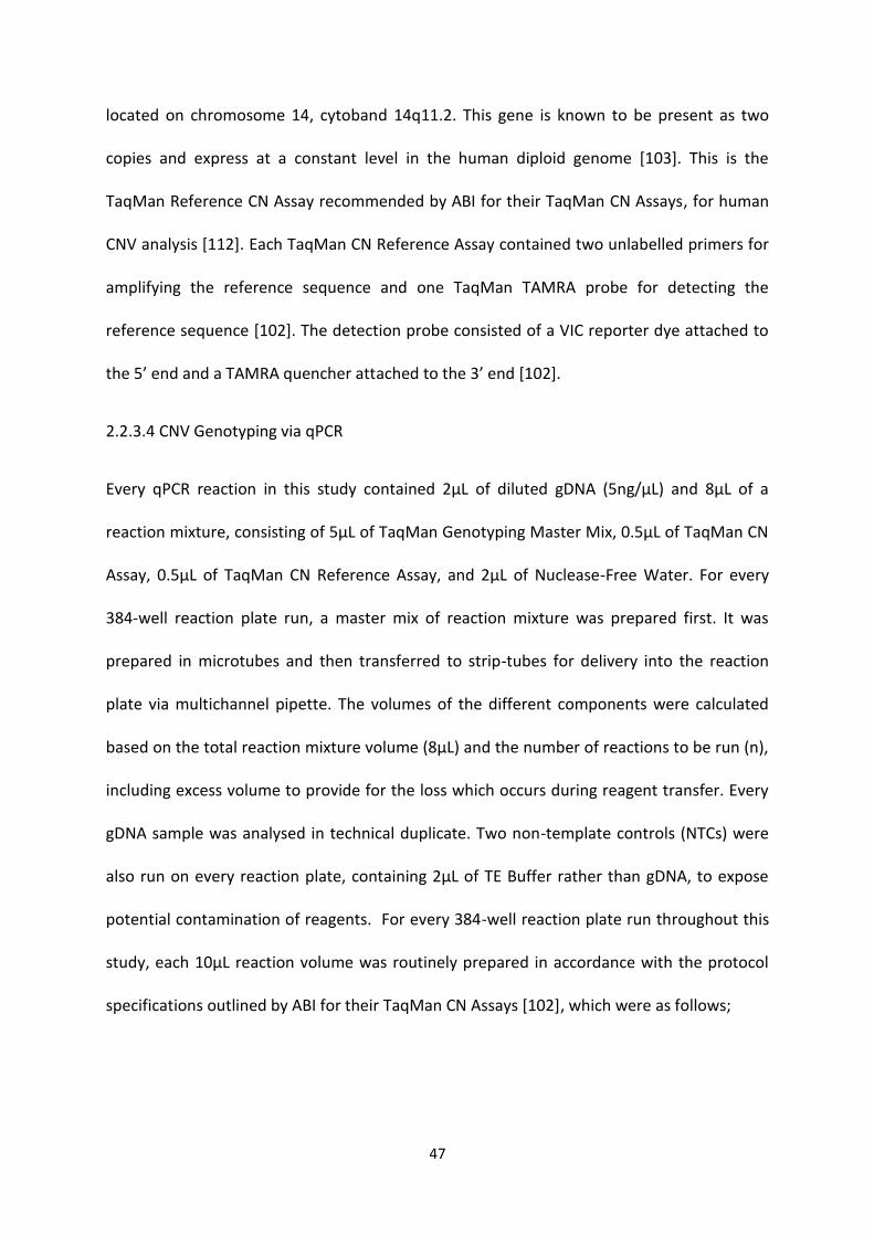
47

located on chromosome 14, cytoband 14q11.2. This gene is known to be present as two

copies and express at a constant level in the human diploid genome [103]. This is the

TaqMan Reference CN Assay recommended by ABI for their TaqMan CN Assays, for human

CNV analysis [112]. Each TaqMan CN Reference Assay contained two unlabelled primers for

amplifying the reference sequence and one TaqMan TAMRA probe for detecting the

reference sequence [102]. The detection probe consisted of a VIC reporter dye attached to

the 5’ end and a TAMRA quencher attached to the 3’ end [102].

2.2.3.4 CNV Genotyping via qPCR

Every qPCR reaction in this study contained 2µL of diluted gDNA (5ng/µL) and 8µL of a

reaction mixture, consisting of 5µL of TaqMan Genotyping Master Mix, 0.5µL of TaqMan CN

Assay, 0.5µL of TaqMan CN Reference Assay, and 2µL of Nuclease-Free Water. For every

384-well reaction plate run, a master mix of reaction mixture was prepared first. It was

prepared in microtubes and then transferred to strip-tubes for delivery into the reaction

plate via multichannel pipette. The volumes of the different components were calculated

based on the total reaction mixture volume (8µL) and the number of reactions to be run (n),

including excess volume to provide for the loss which occurs during reagent transfer. Every

gDNA sample was analysed in technical duplicate. Two non-template controls (NTCs) were

also run on every reaction plate, containing 2µL of TE Buffer rather than gDNA, to expose

potential contamination of reagents. For every 384-well reaction plate run throughout this

study, each 10µL reaction volume was routinely prepared in accordance with the protocol

specifications outlined by ABI for their TaqMan CN Assays [102], which were as follows;

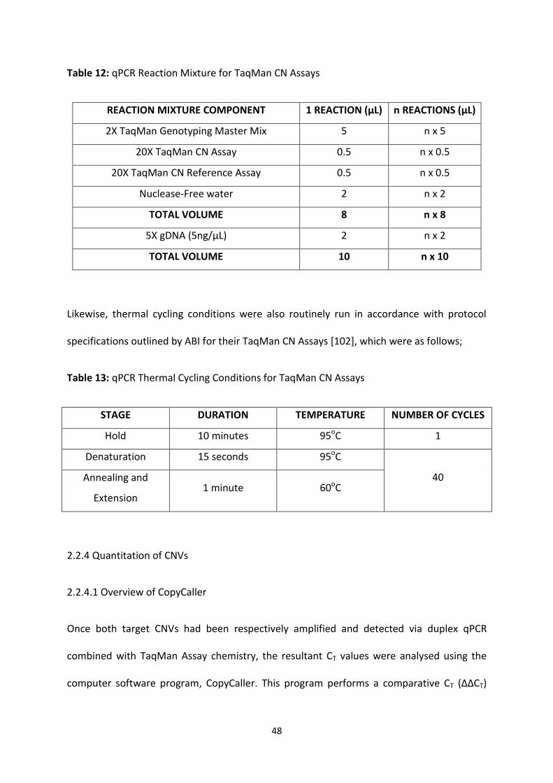
48

Table 12: qPCR Reaction Mixture for TaqMan CN Assays

REACTION MIXTURE COMPONENT 1 REACTION (μL) n REACTIONS (μL)

2X TaqMan Genotyping Master Mix 5 n x 5

20X TaqMan CN Assay 0.5 n x 0.5

20X TaqMan CN Reference Assay 0.5 n x 0.5

Nuclease-Free water 2 n x 2

TOTAL VOLUME 8 n x 8

5X gDNA (5ng/μL) 2 n x 2

TOTAL VOLUME 10 n x 10

Likewise, thermal cycling conditions were also routinely run in accordance with protocol

specifications outlined by ABI for their TaqMan CN Assays [102], which were as follows;

Table 13: qPCR Thermal Cycling Conditions for TaqMan CN Assays

STAGE DURATION TEMPERATURE NUMBER OF CYCLES

Hold 10 minutes 95oC 1

Denaturation 15 seconds 95oC

40 Annealing and

Extension 1 minute 60oC

2.2.4 Quantitation of CNVs

2.2.4.1 Overview of CopyCaller

Once both target CNVs had been respectively amplified and detected via duplex qPCR

combined with TaqMan Assay chemistry, the resultant CT values were analysed using the

computer software program, CopyCaller. This program performs a comparative CT (ΔΔCT)

49

relative quantitation analysis of the qPCR data from the TaqMan CN Assay experiment [113].

In brief, an in-built algorithm automatically determines the CN of the target sequence in

each test gDNA sample, along with related confidence measures. The program first

calculates the difference between the CT values (ΔCT) of the target sequence (of unknown

CN) and the endogenous reference sequence (of known and invariant CN) [113]. Then, the

program compares the ΔCT values of each test sample with that of a calibrator sample that

contains a known number of copies of the target sequence [113]. Alternatively, the analysis

can be performed without the use of a calibrator sample, provided that the predicted CN

distribution, and hence the most frequent CN expected, is known [113]. In this study, due to

time constraints, a control sample could not be identified for either CNV. Therefore,

analyses were performed without the use of a calibrator sample. The most frequent CN

expected for both genes was the wild-type number of copies expected in the human diploid

genome (i.e. CN2) [83].

The quantitative analysis performed by CopyCaller is based on a theoretical model that

describes the exponential nature of the qPCR process [113]. In theory, as the number of

gene copies increases, the difference between successive CT values decreases [107]. In

practice, however, deviations from the ideal may occur, where wells produce ΔCT values

that differ significantly from the mean of all applicable wells [113; 114]. Such deviations can

be attributed to samples that amplify insufficiently or not at all due to experimental error,

such as pipetting inaccuracy, contamination, thermal fluctuations, the binding behaviours of

PCR primers and TaqMan probes, or the starting gDNA concentration of a sample [113;

114]. Nonetheless, the software combined with TaqMan Assay chemistry handles deviations

from the ideal statistical model through the use of an endogenous reference, which detects

50

and removes invalid data and outliers contributing to ΔCT variation [113]. For example, the

program removes background fluorescence by normalising the CT value of each target

sequence with that of the corresponding reference sequence by calculating the well-level CT

difference between each combination [113]. Moreover, a VIC CT value greater than 32.0

indicates failed amplification and the sample is therefore defined as having an

‘undetermined’ CN [113].

CopyCaller is the method of quantitative analysis recommended by ABI for their TaqMan CN

Assays [112]. The program is highly advantageous for quantitative CNV analysis compared to

other methods of analysis. Firstly, CopyCaller limits the amount of human manipulation

needed to genotype gDNA samples compared to manually calculating the relative

expression ratio of a target sequence to a reference sequence via the Pfaffl equation. The

Pfaffl equation is extremely time-consuming and highly susceptible to human error,

particularly when dealing with large sample sets. Moreover, CNV determination via the

Pfaffl equation ultimately depends on the judgement of the experimenter by subjecting the

resultant expression ratios to a subjective ‘binning’ method, which imposes defined zones in

which the CNV statuses fall [111]. Secondly, CopyCaller facilitates the easy expedition of

qPCR data [113], eliminating the need for time-consuming and human error-prone manual

data entry into the template. The resultant CT values from qPCR are presented in a .txt file,

which can be exported from a compatible ABI thermal cycler straight into CopyCaller [113],

thereby reducing the chance for data mismanagement. That being said, some data

manipulation of the .txt file is still required before it is analysed by the program, given that

the resultant CT value from qPCR are automatically presented in such a way that technical

replicates corresponding to a single sample are each represented as if they are different,

51

individual samples. Therefore, by changing the ‘sample name’ in the .txt file, replicate data

can be combined to generate a single CN call for the one sample, along with related

confidence measures. Whilst the ABI thermal cycler software already has a feature that

enables the experimenter to indicate which wells of the reaction plate are sample

replicates, this is also a time-consuming and human error-prone process. It would be ideal if

no data manipulation was required and hence a future recommendation for ABI would be to

refine their presentation of CT values, so that replicate data may be efficiently combined

automatically rather than manually, in what is an otherwise quality product.

2.2.5 Critical Evaluation of Experimental Data

2.2.5.1 Tests of Reliability and Reproducibility

Once every sample has been genotyped for the target CNV of ESR1 and AXIN1, respectively,

they had to be approved for use in statistical analysis based on subjective criteria. Firstly,

the distribution of qPCR data between the two technical replicates of a sample had to be

consistent. For each pair of replicates, the mean, SD, and standard error (SE), of the FAM

and VIC signal intensities on the CT scale were calculated and plotted using the computer

software program, Microsoft Excel. Although less than 0.5 SDs above or below the mean is

the ideal measure of confidence [115], this threshold was expanded to less than 1.0 SDs for

this study to allow for a certain degree of leniency due to limiting gDNA stocks, limiting

reagents, and additional time constraints. If a sample had an obviously large SD for its mean,

exceeding 1.0, it was flagged for a second round of genotyping. Secondly, both replicates of

a sample had to have a viable CN predicted by CopyCaller (i.e. an actual number). An

‘undetermined’ CN indicated that the reaction most likely failed due to an insufficient

amount of starting gDNA template [113]. Conversely, an unreasonably large CN indicated

52

that the reaction most likely contained an excessive concentration of starting gDNA

template [113]. Therefore, if either replicate yielded a CN that was ‘undetermined’ or

unusually large, the sample was flagged for a second round of genotyping. Thirdly, both

replicates of a sample had to have the same CN predicted by CopyCaller, which also

matched up with the CN yielded when replicate data were combined in the CopyCaller

template to represent the one sample. Reproducible data signified a reliable result, so if

there was consistency in CN calls between replicates, the sample was defined as having a

‘confirmed’ CN. Conversely, if there was discrepancy in CN calls between replicates, the

sample was defined as having an ‘unconfirmed’ CN and was thus flagged for a second round

of genotyping. Lastly, there were 11 biological replicates for 9 specific subjects that were

randomly included in the sample set, which served as internal calibrators to validate or

refute CN calls.

2.2.5.2 Prioritisation of Samples with ‘Unconfirmed’ CN from First Round of Genotyping

After the first round of genotyping, reagents for the ESR1 CNV were not limiting and

therefore every sample with an ‘unconfirmed’ CN for the ESR1 CNV could be analysed by

qPCR and CopyCaller again. Conversely, due to limiting reagents for the AXIN1 CNV, as well

as limiting gDNA stocks and additional time constraints, samples with an ‘unconfirmed’ CN

for the AXIN1 CNV had to be prioritised based on the likelihood that results would be

reliable and reproducible when analysed again (Refer to Section 2.2.5.1). Firstly, despite the

discrepancy in CN calls from the first round of genotyping, both technical replicates of a

sample had to have yielded an actual CN (i.e. not ‘undetermined’ by CopyCaller). If either

replicate yielded an ‘undetermined’ CN, it was conceded that its reaction had failed and

would most likely fail again, and the sample was therefore completely eliminated from

53

further analysis of the subject cohort. Secondly, the CN statuses observed from the first

round of genotyping had to be reasonable within the context of this study, considering that

variation from the apparent wild-type CN of the AXIN1 gene in a human diploid genome

(CN2) was expected to represent either heterozygous loss (CN1) or gain (CN3); and more

specifically, the AXIN1 CNV Variant_4912 constitutes a CN loss (CN1). If the aforementioned

criteria were met, it would indicate that the TaqMan CN Assay experiments had worked and

the gDNA stocks were of sufficient quality and quantity for a second round of genotyping.

There was no point in wasting limiting reagents on limiting gDNA stocks if there was not a

strong likelihood of yielding a ‘confirmed’ CN.

2.2.5.3 Prioritisation of Samples with ‘Unconfirmed’ CN from Second Round of Genotyping

After the second round of genotyping, samples which still had an ‘unconfirmed’ CN for ESR1

or AXIN1, respectively, were further prioritised for use in statistical analysis. Due to limiting

gDNA stocks, limiting reagents, and additional time constraints, a third round of genotyping

was simply unfeasible. Moreover, it was important to salvage as many subjects as possible

for statistical analysis, so that the sample size would be large enough to attain sufficient

statistical power, thereby increasing the likelihood of finding statistical significance [116].

Therefore, the remaining samples with an ‘unconfirmed’ CN for ESR1 or AXIN1, respectively,

were subjectively approved for statistical analysis based on the level of confidence that was

estimated by CopyCaller. The program requires a minimum of four technical replicates per

sample to provide a confidence score for a CN call [113]. At this point, the remaining

‘unconfirmed’ samples had been analysed a total of four times (i.e. two rounds of

genotyping as two technical replicates). Therefore, despite the discrepancy in CN calls,

replicate data were combined per sample to yield a single CN call with a related measure of

54

confidence. Although a confidence score between 0.99 and 1.0 is the ideal measure of

confidence [113], this threshold was expanded to between 0.70 and 1.0 for this study, to

allow for a certain degree of leniency due to limiting gDNA stocks, limiting reagents, and

additional time constraints, and so that the maximum possible number of samples could be

approved for statistical analysis.

2.2.6 Statistical Analysis of Experimental Data

2.2.6.1 Consolidation of Genotype and Phenotype Data

Prior to tests of normality and association via SPSS, both the genotype and phenotype data

for every subject had to be consolidated into a common Excel file via the computer software

program, Microsoft Access (i.e. specifically, two separate files for ESR1 CNV and AXIN1 CNV,

respectively). The data required for statistical analysis were the observed CNV genotypes

from this current study and the BMD measurements taken from previous cohort studies.

Data had been recorded across several different Excel files, defined by several different

coded identification numbers pertaining to each subject. Specifically, for each subject, a

GENOS (STH-S) cohort number corresponded to the genotype data and two identification

numbers pertaining to each individual and their family, respectively, corresponded to the

phenotype data. Each subject could be identified according to all three of these unique

numbers. Merging both the genotype and phenotype data into a common source of access

improved traceability and reduced potential mismatches, which facilitated the easy

expedition of selected data into new Excel templates to be exported into SPSS for statistical

analysis.

55

2.2.6.2 Tests of Normality via SPSS

For each analysis of the association between CNV genotype data (i.e. for ESR1 and AXIN1,

respectively) and selected BMD phenotype data (Refer to Section 2.2.2.1), the dataset was

examined for normality via SPSS. Several tests of normality were conducted, which

compared the selected sample data to a normal distribution with the same mean and SD

[119]. The Shapiro-Wilk test of normality tested the null hypothesis of a normally distributed

population [119]. Deviations from normality were statistically significant if the p-value was

less than the 0.05 significance level, in which case the null hypothesis of normal distribution

was rejected. Conversely, if the p-value was greater than the 0.05 significance level, the null

hypothesis of normal distribution was not rejected, thereby indicating normality. Moreover,

normally distributed data would allow association analysis to be conducted using a

parametric test [120]. The results of the Shapiro-Wilk test were further confirmed by

visually screening both Normal Quantile-Quantile (Q-Q) and Box Plots, which are graphical

means of determining the level of normality [119]. The Normal Q-Q Plot for logistic

regression residuals compared the observed dataset with the expected values for a normal

distribution. It highlighted where observed data points deviated from the expected trend-

line, and hence did not display normal distribution; and conversely, where observed data

were consistent with the expected trend-line, and hence contributed to normal distribution.

The Box Plot showed the consistency of the dataset, highlighting where obvious outliers

may have skewed the distribution away from normality; and conversely, where the box plot

was symmetrical and evenly spaced, suggesting normal distribution.

56

2.2.6.3 Tests of Association via SPSS

Tests of association between the CNV genotype data (i.e. ESR1 and AXIN1, respectively) and

selected BMD phenotype data (Refer to Section 2.2.2.1) were conducted via SPSS. Assuming

normally distributed data, three different parametric tests could be performed, depending

on the number of observed CNV genotype groups (i.e. independent variable) and the

selected BMD phenotype (i.e. dependent variable). The precondition of each test was the

Levene’s Test for Equality of Error Variances, which assessed the variance homogeneity. The

Levene’s Test tested the null hypothesis of equal error variance for BMD across the different

CNV genotype groups [119], which was not rejected if the p-value was greater than the

significance level of 0.05, indicating that the assumption of equal variances was met.

Firstly, the potential effect of ESR1 CNV in relation to BMD (g/cm2) and its related BMDZ was

tested using a One-Way ANOVA Test of Between-Subject Effects. This technique is typically

used to compare the means of at least three different sample groups [119]. Therefore, it

was appropriate for testing the potential effect of ESR1 CNV, considering that three

different CNV genotypes were observed; CN loss (CN1), wild-type (CN2), and CN gain (CN3).

The ANOVA test tested the null hypothesis that the difference in mean BMD between the

three CNV genotype groups was no greater than that due to normal variation of subjects’

characteristics, and error in their measurement [119]. The null hypothesis was rejected if

the p-value was less than the 0.05 significance level, which would therefore indicate that

there was evidence of a statistically significant association between CNV and BMD.

Conversely, if the p-value was greater than the 0.05 significance level, the null hypothesis of

equal means was not rejected, which would therefore indicate that there was no evidence

of a statistically significant association between CNV and BMD.

57

Secondly, the potential effect of AXIN1 CNV in relation to BMD (g/cm2) and the related

BMDZ was tested using an Independent-Sample T-test. This technique is typically used to

compare the means of two different sample groups [119]. Therefore, it was appropriate for

testing the potential effect of AXIN1 CNV, considering that only two different CNV

genotypes had available phenotype data for statistical analysis; wild-type (CN2) and CN gain

(CN3). The T-test tested the hypothesis that the difference in mean BMD between the two

CNV genotype groups was no greater than that due to normal variation of subjects’

characteristics, and error in their measurement [119]. The null hypothesis was rejected if

the p-value was less than the 0.05 significance level, which would therefore indicate that

there was evidence of a statistically significant association between CNV and BMD.

Conversely, if the p-value was greater than the 0.05 significance level, the null hypothesis of

equal means was not rejected, which would therefore indicate that there was no evidence

of a statistically significant association between CNV and BMD.

Lastly, the potential effect of several covariates (i.e. age, age2, height, weight, and BMI) in

relation to the association between CNV (i.e. ESR1 and AXIN1, respectively) and BMD

(g/cm2) was tested using an Analysis of Covariance (ANCOVA) test. This technique is a

general linear model which combines ANOVA and regression [119] to evaluate whether the

population means of a dependent variable (i.e. BMD) are equal across groups of a

categorical independent variable (i.e. CNV genotype groups), while statistically controlling

for the effects of other continuous variables that are not of primary interest (i.e. covariates)

[119]. The ANCOVA test tested the hypothesis that there was no difference in mean BMD

between the different CNV genotype groups, which was rejected if the p-value was less than

the 0.05 significance level, indicating that there was evidence of a statistically significant

58

association between CNV, BMD, and covariates. Conversely, if the p-value was greater than

the 0.05 significance level, the null hypothesis of equal means was not rejected, which

would indicate that there was no evidence of a statistically significant association between

CNV, BMD, and covariates.

59

Chapter 3: Analysis of ESR1 CNV and BMD

60

3.1 Introduction

The oestrogen receptor 1 (ESR1) gene is one of the most extensively studied candidate

genes for involvement in the regulation of bone. Several common genetic variants in the

ESR1 gene have been described and are widely anticipated to contribute to phenotypic

diversity of bone traits. For example, previous studies have identified three polymorphic

sites in the 5’ end of the gene: a (TA)n variable number tandem repeat (VNTR) located

approximately 1kb upstream of exon 1, and the PvuII and XbaI restriction fragment length

polymorphisms (RFLPs) in intron 1, about 400 bp upstream of exon 2 [49]. Associations of

these polymorphisms with bone traits have been reported, but results have been largely

inconsistent between studies [49]. Nonetheless, several large-scale analysis projects firmly

implicate genetic variations of ESR1 with BMD, thereby providing insights into the potential

functional role that ESR1 plays in bone regulation. For example, a meta-analysis of five

GWAS of BMD in 19,195 subjects (including 14,277 women of European descent) identified

a total of 54 SNPs in intron 1 of ESR1 in statistically significant association with BMD, of

which 36 SNPs were associated with lumbar spine BMD (lowest p value: 6.1 x 10-11) and the

remaining 18 SNPs were associated with femoral neck BMD (lowest p value: 3.0 x 10-8) [98].

Moreover, these findings are comparable to those of similar studies [19; 121]. In view of

this, there appears to be sufficient evidence to suggest that ESR1 may play an important

role in bone regulation at multiple skeletal sites; however, the accurate elucidation of this

depends on the biological plausibility.

According to the UCSC Genome Browser, the ESR1 gene is 412,778 bp in length and is

located on the cytoband 6q25.1c. It encodes the oestrogen receptor isoform, oestrogen

receptor-α, which is a ligand-activated transcription factor expressed in bone marrow-

61

derived cells [122], such as osteoclasts, osteoblasts, osteocytes (a final differentiated cell

type of the osteoblast lineage), and bone marrow stromal cells [6]. Previous studies

highlight a role for ESR1 as a mediator for the response of target cells to the effects of the

reproductive steroid hormone, oestrogen [19]. In brief, being a typical steroid hormone,

oestrogen can elicit a cellular response via direct and indirect regulation of gene expression.

Direct regulation of gene expression involves the diffusion of oestrogen through the cellular

membrane, where it binds to and activates its intracellular receptor, which then interacts

with the hormone-response and regulatory elements of oestrogen-responsive genes,

thereby initiating their transcription [123]. Indirect regulation of gene expression involves

oestrogen binding to either steroid or non-steroid receptors, which induces kinase signalling

pathways [124]. In view of this, it can be reasonably assumed that ESR1 may regulate the

transcription of genes relevant to bone regulation, in response to oestrogen.

It is well documented that oestrogen is essential for healthy bone turnover. Like the other

reproductive steroid hormones, it is a key regulator of osteoblast differentiation [125].

Although oestrogen has been shown to up-regulate the expression of osteoblastogenic

markers in mesenchymal stem cells (MSCs) (i.e. RUNX2, ALPL, and COL1) [126] and promote

the deposition of new bone, extensive clinical research indicates that the main effect of

oestrogen on the promotion of bone formation actually lies in its inhibition of osteoclast

differentiation [5; 127]. Therefore, oestrogen essentially promotes the protection against

bone loss. For example, a study conducted by Bord et al in 2003 documented that human

osteoblasts respond to low dose oestrogen treatment with the repression of RANKL, whilst

maintaining the expression of the decoy ligand, OPG [128]. This suggests that oestrogen

may inhibit RANKL from binding to RANK on osteoclast precursors by promoting down-

62

regulation of RANKL and up-regulation of OPG, which inhibits the activation of osteoclasts,

thereby protecting against bone loss. Moreover, evidence that oestrogen also modulates

cytokines (i.e. IL-6, IL-1, and TNF-α) and growth factors (i.e. TGF-β), coupled with evidence

that these factors are potential mediators of osteoclast differentiation [129], even further

highlights the critical role that oestrogen plays in bone regulation.

Previous studies have firmly demonstrated that oestrogen has positive effects on bone

regulation, including bone turnover, acquisition of peak bone mass, and inhibition of bone

loss [130]. In view of this, it appears reasonable to assume that oestrogen protects against

osteoporosis. There are several lines of evidence supporting the role of oestrogen deficiency

in osteoporosis. For example, postmenopausal women, whose oestrogen levels naturally

decline, are known to be at the highest risk of developing the disease [19]. Moreover,

women experience accelerated bone loss at a rate of 3 to 5% per year during menopause

[25], which studies attribute to accelerated bone remodelling, as indicated by an increase in

the levels of biological markers related to bone resorption and formation [5]. Consistent

with this, oestrogen replacement in early menopausal women has been shown to decrease

the risk of osteoporotic fractures [49]. Therefore, there is strong evidence implicating

oestrogen deficiency with osteoporosis.

In view of existing evidence highlighting the activity of the ESR1 gene, the oestrogen

receptor-α, and oestrogen, it appears reasonable to assume that the normal, human diploid

wild-type expression of ESR1 encodes a functional oestrogen receptor which mediates the

response of target cells to oestrogen, thereby producing a phenotype which is consistent

with healthy bone maintenance (i.e. high BMD and low fracture risk). Therefore, a loss or

gain of ESR1 sequence in relation to ESR1 CNV may consequently cause a loss-of-function or

63

gain-of-function mutation, respectively, which may disrupt the transcriptional control of

ESR1 or other genes. For example, a loss-of-function mutation in relation to ESR1 CNV may

encode an altered oestrogen receptor-α which is no longer responsive to oestrogen and

therefore does not offer protection against bone loss, thereby producing a phenotype which

is consistent with an increased risk of osteoporosis. Conversely, a gain-of-function mutation

in relation to ESR1 CNV may encode an altered receptor which enhances the protection

against bone loss or may even have long-range positional effects on the transcriptional

control of other genes which have completely different functional roles all together.

Nonetheless, the exact functional roles of both ESR1 and CNV remain to be fully elucidated

and therefore gains and losses of function in relation to ESR1 CNV are currently difficult to

interpret.

According to the DGV, there are several known CNVs for the ESR1 gene. The ESR1 CNV

identified as Variant_4512 was analysed in this study. Variant_4512 is a genomic sequence

222,242 bp in length and constitutes a gain in ESR1 CN [131]. It was previously discovered by

Wong et al in 2007 using the bacterial artificial chromosome (BAC) array CGH analysis

method [131]. It was selected for analysis in this current study based on criteria outlined in

Section 2.2.1, but also because it encompasses the 5’ end of ESR1, where the promoter

sequence and regulatory elements are expected to be located [130], which therefore

implicates gene expression. Furthermore, several genetic variations of the ESR1 mRNA

transcript, such as those located in the 5’ end, have already been implicated in association

with phenotypes related to the risk of osteoporosis, such as BMD [49]. According to the

UCSC Genome Browser, and highlighted in Figure 3, Variant_4512 does not encompass the

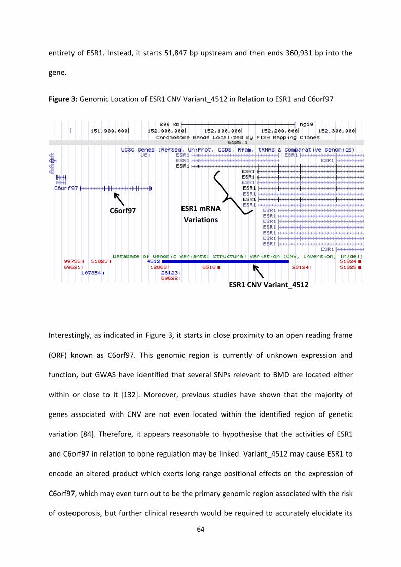
64

entirety of ESR1. Instead, it starts 51,847 bp upstream and then ends 360,931 bp into the

gene.

Figure 3: Genomic Location of ESR1 CNV Variant_4512 in Relation to ESR1 and C6orf97

Interestingly, as indicated in Figure 3, it starts in close proximity to an open reading frame

(ORF) known as C6orf97. This genomic region is currently of unknown expression and

function, but GWAS have identified that several SNPs relevant to BMD are located either

within or close to it [132]. Moreover, previous studies have shown that the majority of

genes associated with CNV are not even located within the identified region of genetic

variation [84]. Therefore, it appears reasonable to hypothesise that the activities of ESR1

and C6orf97 in relation to bone regulation may be linked. Variant_4512 may cause ESR1 to

encode an altered product which exerts long-range positional effects on the expression of

C6orf97, which may even turn out to be the primary genomic region associated with the risk

of osteoporosis, but further clinical research would be required to accurately elucidate its

C6orf97

ESR1 CNV Variant_4512

ESR1 mRNA

Variations

65

role. Nonetheless, considering that several genetic variations in the 5’ end of ESR1 have

already been implicated in bone regulation, Variant_4512 seemed an appropriate CNV for

investigating the potential association between ESR1 CNV and osteoporosis.

66

3.2 Materials and Methods

This study investigated the potential effect of two different CNVs on BMD, and although the

CNVs were analysed separately, all methods were applied in exactly the same manner,


CNV are collectively described in a general methods section (Refer to Chapter 2: Materials

and Methods).

67

3.3 Results

3.3.1 Quality Control

The first measure of quality control of the experimental data was that no TaqMan signals

were detected for DNA amplification in the NTC wells of every 384-well qPCR reaction plate

run. qPCR data were examined for consistency and confidence between the two technical

replicates of every analysed sample using the mean, SD, and SE, of the FAM and VIC signal

intensities on the CT scale. By criteria modified for this study (Refer to Section 2.2.5.1),

normally distributed data were located less than 1.0 SD above or below the mean. The

majority of analysed samples had a SD below 1.0, so they were within the acceptable

threshold, and were thus approved for statistical analysis. Higher SD tended to correlate

with a higher degree of variability displayed by the VIC signals, which were generally more

variable than the FAM signals. Several samples had a SD exceeding 1.0 and they were

defined as having an ‘unconfirmed’ CN (even if both technical replicates had the same CN

predicted by CopyCaller). ‘Unconfirmed’ samples were subjected to a second round of

genotyping, which in turn yielded an acceptable SD. Therefore, it was reasonably accepted

that the majority of qPCR data in this study were sufficiently reproducible and reliable for

CN assignment by CopyCaller.

CopyCaller results were then examined for consistency and confidence between the two

technical replicates of every analysed sample. By criteria modified for this study (Refer to

Section 2.2.5.1), a ‘confirmed’ CN was assigned to a sample if both replicates were assigned

the same CN and it also matched up with the CN yielded when replicate data were

combined to represent a single sample. Although CopyCaller could not produce a

confidence score for only two replicates, the proven reproducibility of the qPCR data

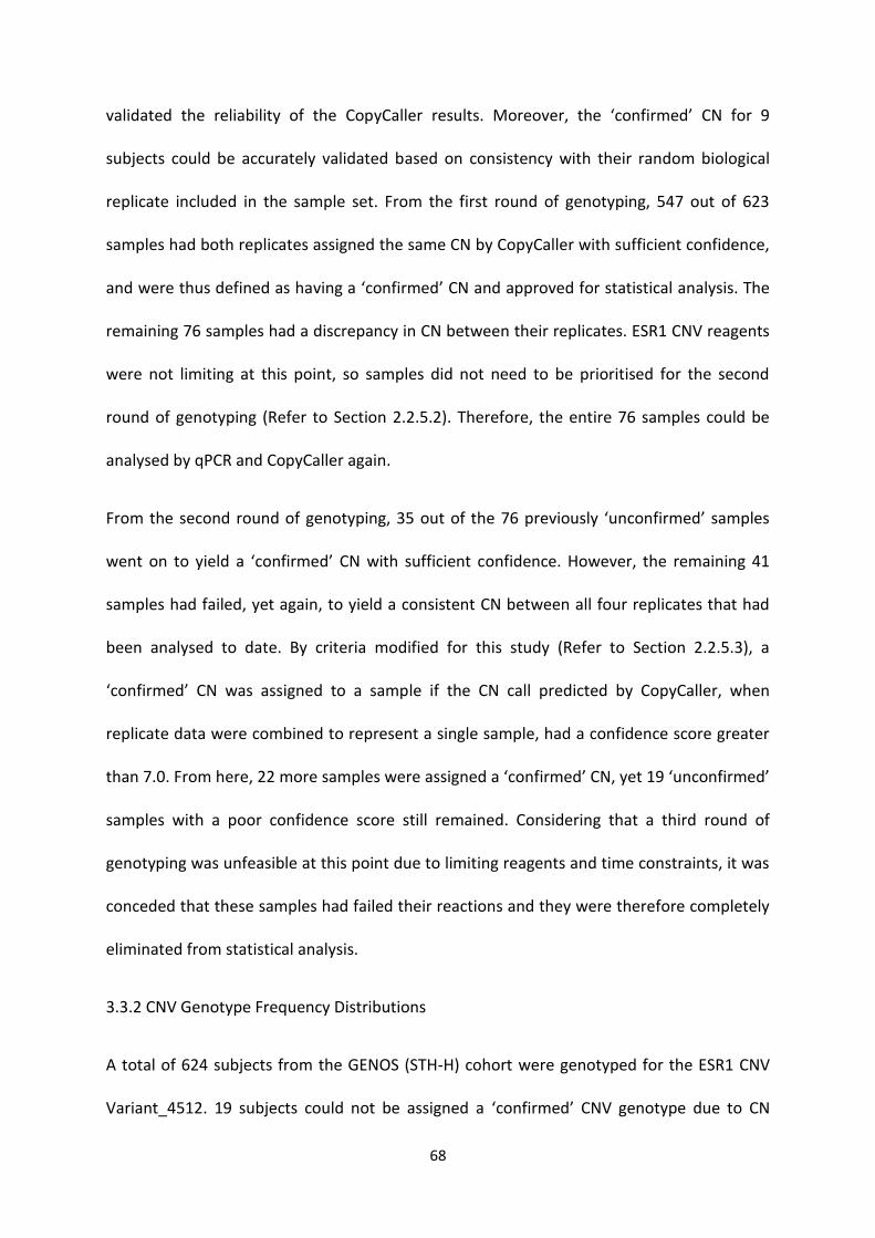
68

validated the reliability of the CopyCaller results. Moreover, the ‘confirmed’ CN for 9

subjects could be accurately validated based on consistency with their random biological

replicate included in the sample set. From the first round of genotyping, 547 out of 623

samples had both replicates assigned the same CN by CopyCaller with sufficient confidence,

and were thus defined as having a ‘confirmed’ CN and approved for statistical analysis. The

remaining 76 samples had a discrepancy in CN between their replicates. ESR1 CNV reagents

were not limiting at this point, so samples did not need to be prioritised for the second

round of genotyping (Refer to Section 2.2.5.2). Therefore, the entire 76 samples could be

analysed by qPCR and CopyCaller again.

From the second round of genotyping, 35 out of the 76 previously ‘unconfirmed’ samples

went on to yield a ‘confirmed’ CN with sufficient confidence. However, the remaining 41

samples had failed, yet again, to yield a consistent CN between all four replicates that had

been analysed to date. By criteria modified for this study (Refer to Section 2.2.5.3), a

‘confirmed’ CN was assigned to a sample if the CN call predicted by CopyCaller, when

replicate data were combined to represent a single sample, had a confidence score greater

than 7.0. From here, 22 more samples were assigned a ‘confirmed’ CN, yet 19 ‘unconfirmed’

samples with a poor confidence score still remained. Considering that a third round of

genotyping was unfeasible at this point due to limiting reagents and time constraints, it was

conceded that these samples had failed their reactions and they were therefore completely

eliminated from statistical analysis.

3.3.2 CNV Genotype Frequency Distributions

A total of 624 subjects from the GENOS (STH-H) cohort were genotyped for the ESR1 CNV

Variant_4512. 19 subjects could not be assigned a ‘confirmed’ CNV genotype due to CN

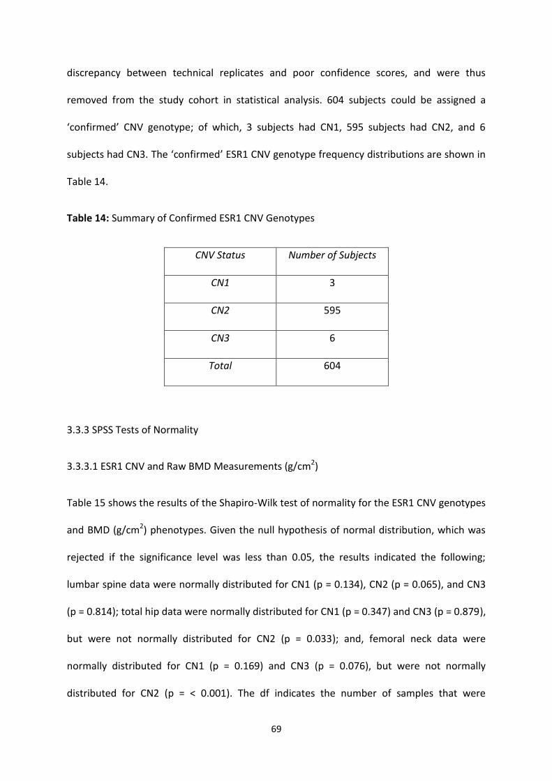
69

discrepancy between technical replicates and poor confidence scores, and were thus

removed from the study cohort in statistical analysis. 604 subjects could be assigned a

‘confirmed’ CNV genotype; of which, 3 subjects had CN1, 595 subjects had CN2, and 6

subjects had CN3. The ‘confirmed’ ESR1 CNV genotype frequency distributions are shown in

Table 14.

Table 14: Summary of Confirmed ESR1 CNV Genotypes

CNV Status Number of Subjects

CN1 3

CN2 595

CN3 6

Total 604

3.3.3 SPSS Tests of Normality

3.3.3.1 ESR1 CNV and Raw BMD Measurements (g/cm2)

Table 15 shows the results of the Shapiro-Wilk test of normality for the ESR1 CNV genotypes

and BMD (g/cm2) phenotypes. Given the null hypothesis of normal distribution, which was

rejected if the significance level was less than 0.05, the results indicated the following;

lumbar spine data were normally distributed for CN1 (p = 0.134), CN2 (p = 0.065), and CN3

(p = 0.814); total hip data were normally distributed for CN1 (p = 0.347) and CN3 (p = 0.879),

but were not normally distributed for CN2 (p = 0.033); and, femoral neck data were

normally distributed for CN1 (p = 0.169) and CN3 (p = 0.076), but were not normally

distributed for CN2 (p = < 0.001). The df indicates the number of samples that were

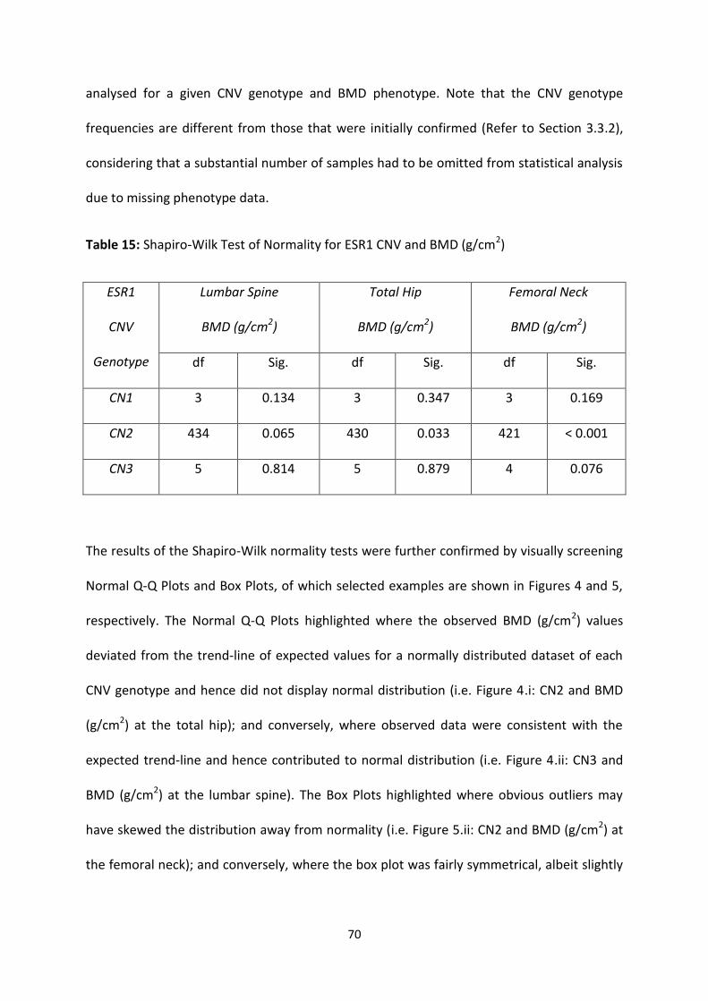
70

analysed for a given CNV genotype and BMD phenotype. Note that the CNV genotype

frequencies are different from those that were initially confirmed (Refer to Section 3.3.2),

considering that a substantial number of samples had to be omitted from statistical analysis

due to missing phenotype data.

Table 15: Shapiro-Wilk Test of Normality for ESR1 CNV and BMD (g/cm2)

ESR1

CNV

Genotype

Lumbar Spine

BMD (g/cm2)

Total Hip

BMD (g/cm2)

Femoral Neck

BMD (g/cm2)

df Sig. df Sig. df Sig.

CN1 3 0.134 3 0.347 3 0.169

CN2 434 0.065 430 0.033 421 < 0.001

CN3 5 0.814 5 0.879 4 0.076

The results of the Shapiro-Wilk normality tests were further confirmed by visually screening

Normal Q-Q Plots and Box Plots, of which selected examples are shown in Figures 4 and 5,

respectively. The Normal Q-Q Plots highlighted where the observed BMD (g/cm2) values

deviated from the trend-line of expected values for a normally distributed dataset of each

CNV genotype and hence did not display normal distribution (i.e. Figure 4.i: CN2 and BMD

(g/cm2) at the total hip); and conversely, where observed data were consistent with the

expected trend-line and hence contributed to normal distribution (i.e. Figure 4.ii: CN3 and

BMD (g/cm2) at the lumbar spine). The Box Plots highlighted where obvious outliers may

have skewed the distribution away from normality (i.e. Figure 5.ii: CN2 and BMD (g/cm2) at

the femoral neck); and conversely, where the box plot was fairly symmetrical, albeit slightly

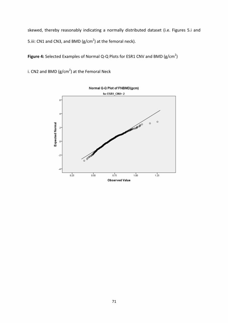
71

skewed, thereby reasonably indicating a normally distributed dataset (i.e. Figures 5.i and

5.iii: CN1 and CN3, and BMD (g/cm2) at the femoral neck).

Figure 4: Selected Examples of Normal Q-Q Plots for ESR1 CNV and BMD (g/cm2)

i. CN2 and BMD (g/cm2) at the Femoral Neck

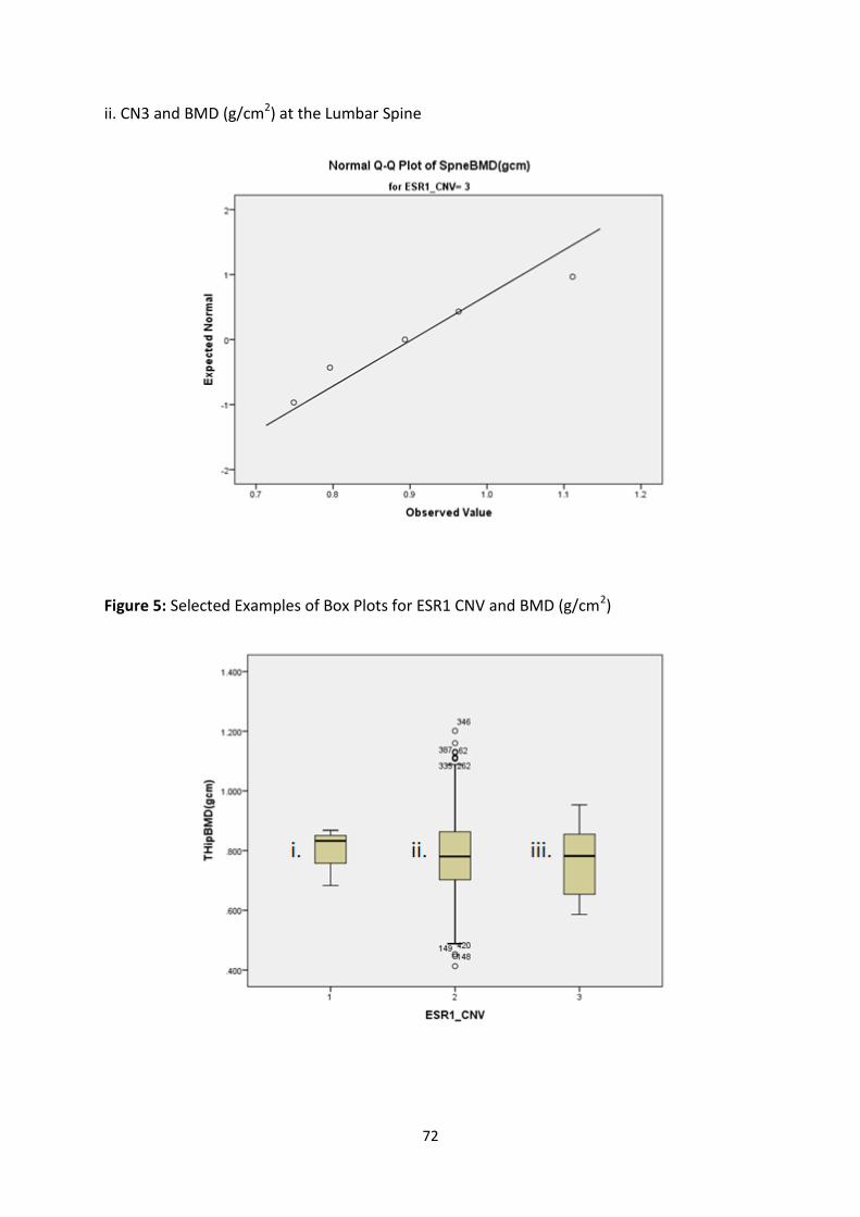
72

ii. CN3 and BMD (g/cm2) at the Lumbar Spine

Figure 5: Selected Examples of Box Plots for ESR1 CNV and BMD (g/cm2)

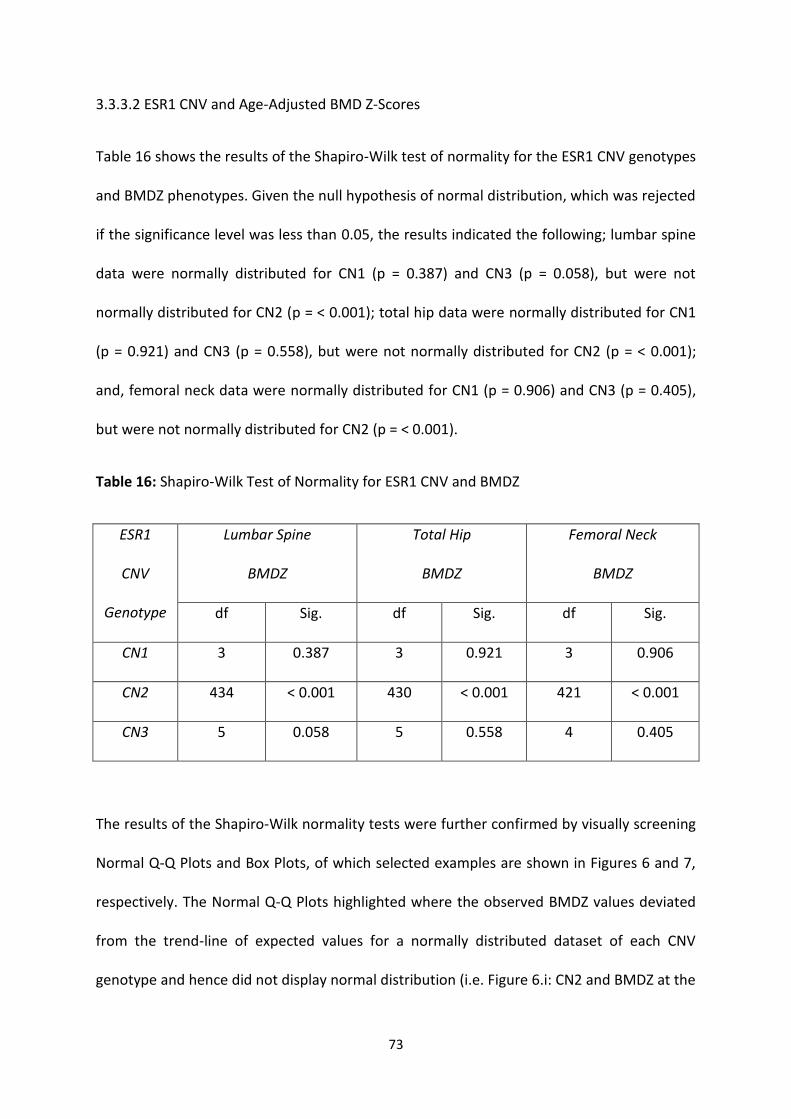
73

3.3.3.2 ESR1 CNV and Age-Adjusted BMD Z-Scores

Table 16 shows the results of the Shapiro-Wilk test of normality for the ESR1 CNV genotypes

and BMDZ phenotypes. Given the null hypothesis of normal distribution, which was rejected

if the significance level was less than 0.05, the results indicated the following; lumbar spine

data were normally distributed for CN1 (p = 0.387) and CN3 (p = 0.058), but were not

normally distributed for CN2 (p = < 0.001); total hip data were normally distributed for CN1

(p = 0.921) and CN3 (p = 0.558), but were not normally distributed for CN2 (p = < 0.001);

and, femoral neck data were normally distributed for CN1 (p = 0.906) and CN3 (p = 0.405),

but were not normally distributed for CN2 (p = < 0.001).

Table 16: Shapiro-Wilk Test of Normality for ESR1 CNV and BMDZ

ESR1

CNV

Genotype

Lumbar Spine

BMDZ

Total Hip

BMDZ

Femoral Neck

BMDZ


CN1 3 0.387 3 0.921 3 0.906

CN2 434 < 0.001 430 < 0.001 421 < 0.001

CN3 5 0.058 5 0.558 4 0.405



respectively. The Normal Q-Q Plots highlighted where the observed BMDZ values deviated

from the trend-line of expected values for a normally distributed dataset of each CNV

genotype and hence did not display normal distribution (i.e. Figure 6.i: CN2 and BMDZ at the

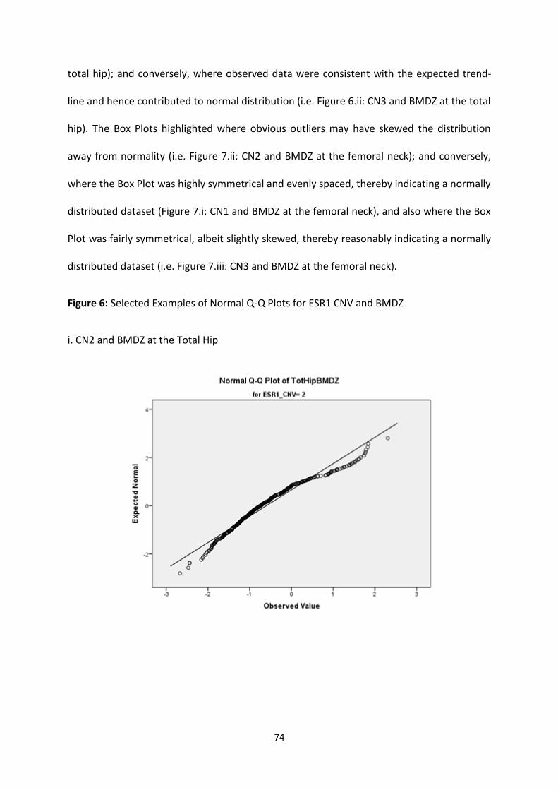
74

total hip); and conversely, where observed data were consistent with the expected trend-

line and hence contributed to normal distribution (i.e. Figure 6.ii: CN3 and BMDZ at the total

hip). The Box Plots highlighted where obvious outliers may have skewed the distribution

away from normality (i.e. Figure 7.ii: CN2 and BMDZ at the femoral neck); and conversely,

where the Box Plot was highly symmetrical and evenly spaced, thereby indicating a normally

distributed dataset (Figure 7.i: CN1 and BMDZ at the femoral neck), and also where the Box

Plot was fairly symmetrical, albeit slightly skewed, thereby reasonably indicating a normally

distributed dataset (i.e. Figure 7.iii: CN3 and BMDZ at the femoral neck).

Figure 6: Selected Examples of Normal Q-Q Plots for ESR1 CNV and BMDZ

i. CN2 and BMDZ at the Total Hip

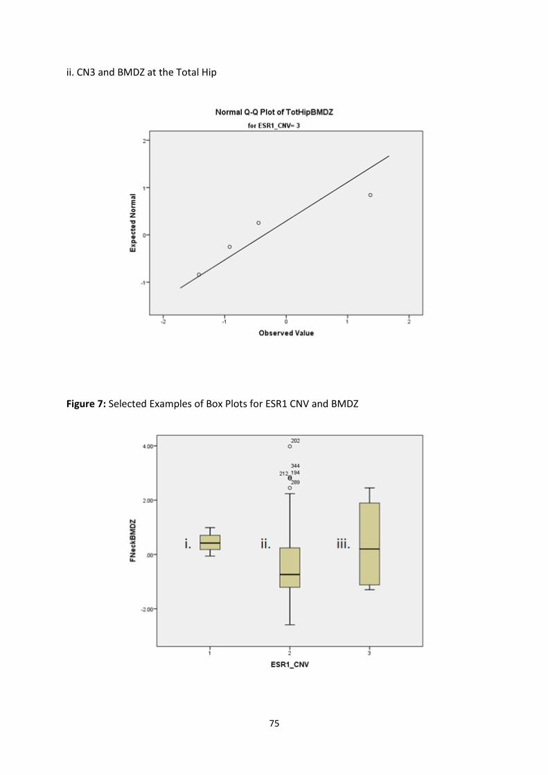
75

ii. CN3 and BMDZ at the Total Hip

Figure 7: Selected Examples of Box Plots for ESR1 CNV and BMDZ

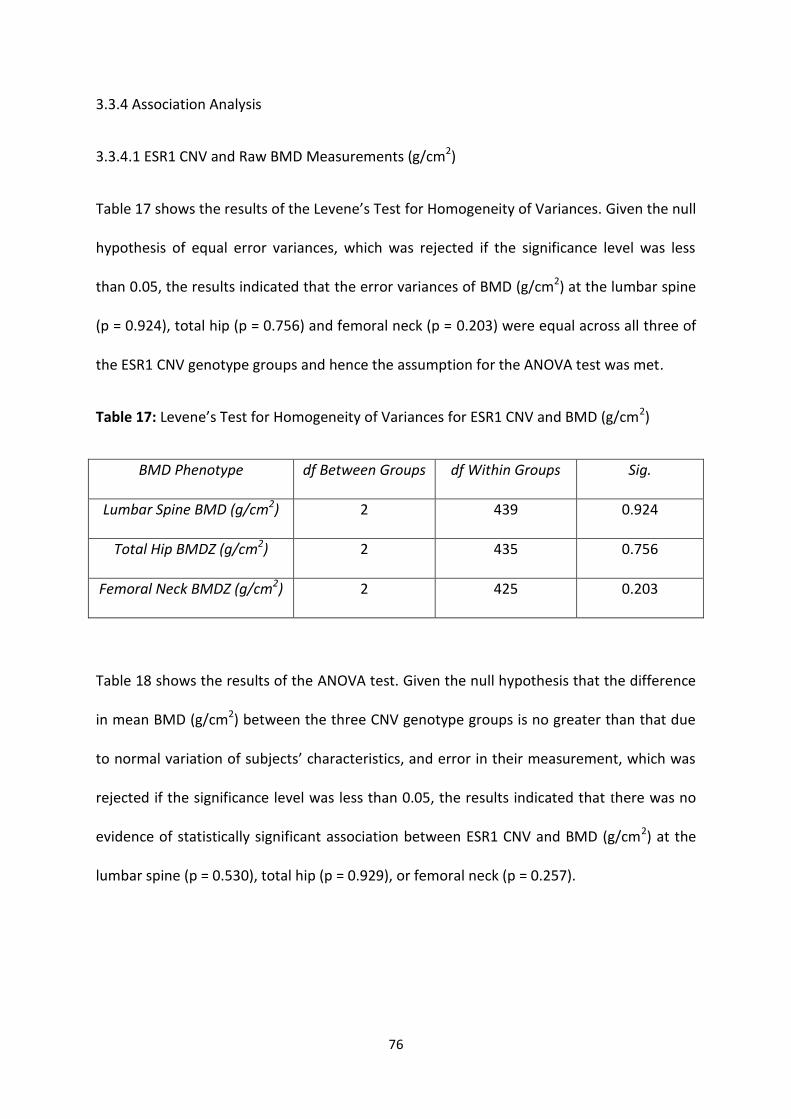
76

3.3.4 Association Analysis

3.3.4.1 ESR1 CNV and Raw BMD Measurements (g/cm2)

Table 17 shows the results of the Levene’s Test for Homogeneity of Variances. Given the null

hypothesis of equal error variances, which was rejected if the significance level was less

than 0.05, the results indicated that the error variances of BMD (g/cm2) at the lumbar spine

(p = 0.924), total hip (p = 0.756) and femoral neck (p = 0.203) were equal across all three of

the ESR1 CNV genotype groups and hence the assumption for the ANOVA test was met.

Table 17: Levene’s Test for Homogeneity of Variances for ESR1 CNV and BMD (g/cm2)

BMD Phenotype df Between Groups df Within Groups Sig.

Lumbar Spine BMD (g/cm2) 2 439 0.924

Total Hip BMDZ (g/cm2) 2 435 0.756

Femoral Neck BMDZ (g/cm2) 2 425 0.203

Table 18 shows the results of the ANOVA test. Given the null hypothesis that the difference

in mean BMD (g/cm2) between the three CNV genotype groups is no greater than that due

to normal variation of subjects’ characteristics, and error in their measurement, which was

rejected if the significance level was less than 0.05, the results indicated that there was no

evidence of statistically significant association between ESR1 CNV and BMD (g/cm2) at the

lumbar spine (p = 0.530), total hip (p = 0.929), or femoral neck (p = 0.257).

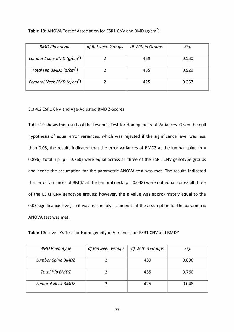
77

Table 18: ANOVA Test of Association for ESR1 CNV and BMD (g/cm2)



Total Hip BMDZ (g/cm2) 2 435 0.929

Femoral Neck BMD (g/cm2) 2 425 0.257

3.3.4.2 ESR1 CNV and Age-Adjusted BMD Z-Scores



than 0.05, the results indicated that the error variances of BMDZ at the lumbar spine (p =

0.896), total hip (p = 0.760) were equal across all three of the ESR1 CNV genotype groups

and hence the assumption for the parametric ANOVA test was met. The results indicated

that error variances of BMDZ at the femoral neck (p = 0.048) were not equal across all three

of the ESR1 CNV genotype groups; however, the p value was approximately equal to the

0.05 significance level, so it was reasonably assumed that the assumption for the parametric

ANOVA test was met.

Table 19: Levene’s Test for Homogeneity of Variances for ESR1 CNV and BMDZ


Lumbar Spine BMDZ 2 439 0.896

Total Hip BMDZ 2 435 0.760

Femoral Neck BMDZ 2 425 0.048

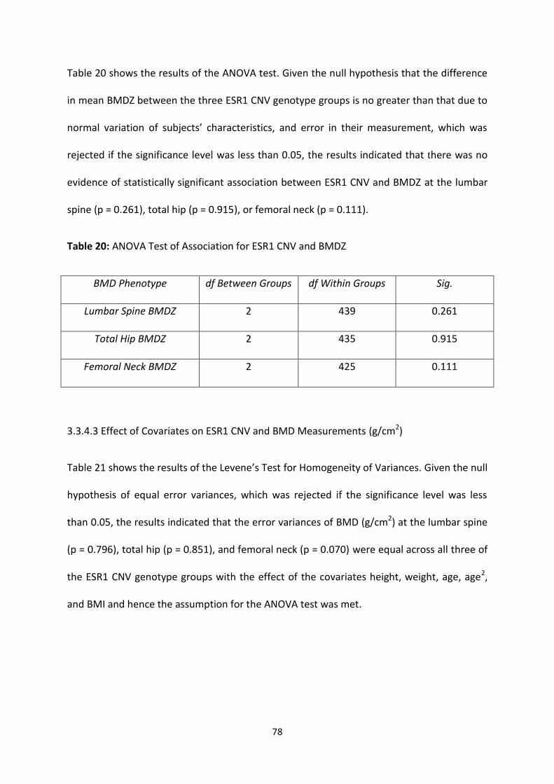
78

Table 20 shows the results of the ANOVA test. Given the null hypothesis that the difference

in mean BMDZ between the three ESR1 CNV genotype groups is no greater than that due to

normal variation of subjects’ characteristics, and error in their measurement, which was


evidence of statistically significant association between ESR1 CNV and BMDZ at the lumbar

spine (p = 0.261), total hip (p = 0.915), or femoral neck (p = 0.111).

Table 20: ANOVA Test of Association for ESR1 CNV and BMDZ





3.3.4.3 Effect of Covariates on ESR1 CNV and BMD Measurements (g/cm2)




(p = 0.796), total hip (p = 0.851), and femoral neck (p = 0.070) were equal across all three of

the ESR1 CNV genotype groups with the effect of the covariates height, weight, age, age2,

and BMI and hence the assumption for the ANOVA test was met.

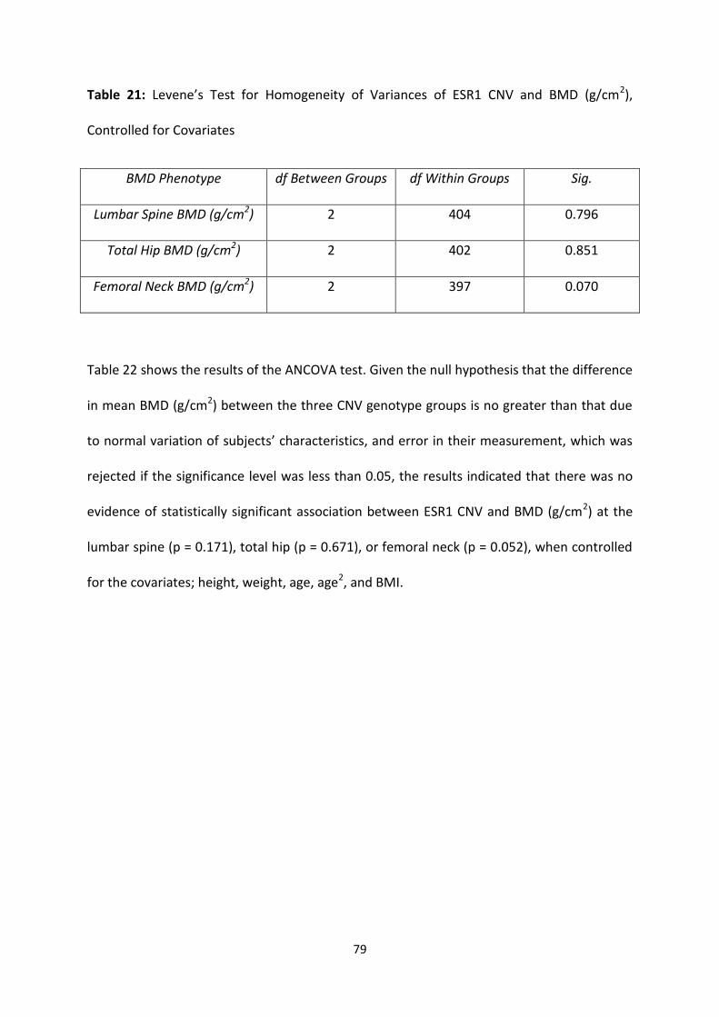
79

Table 21: Levene’s Test for Homogeneity of Variances of ESR1 CNV and BMD (g/cm2),




Total Hip BMD (g/cm2) 2 402 0.851


Table 22 shows the results of the ANCOVA test. Given the null hypothesis that the difference

in mean BMD (g/cm2) between the three CNV genotype groups is no greater than that due

to normal variation of subjects’ characteristics, and error in their measurement, which was


evidence of statistically significant association between ESR1 CNV and BMD (g/cm2) at the

lumbar spine (p = 0.171), total hip (p = 0.671), or femoral neck (p = 0.052), when controlled

for the covariates; height, weight, age, age2, and BMI.

80

Table 22: ANCOVA Test of Association for ESR1 CNV and BMD (g/cm2), Controlled for

Covariates

BMD

Phenotype

Lumbar Spine BMD

(g/cm2)

Total Hip BMD

(g/cm2)

Femoral Neck BMD

(g/cm2)

Covariate df Sig. df Sig. df Sig.

Height 1 0.303 1 0.904 1 0.119

Weight 1 0.042 1 0.404 1 0.009

Age 1 0.146 1 0.117 1 < 0.001

Age2 1 0.002 1 0.630 1 0.100

BMI 1 0.121 1 0.994 1 0.070

ESR1 CNV 2 0.171 2 0.671 2 0.052

81

3.4 Discussion

This study investigated the potential effect of CNV in the pathogenesis of osteoporosis, with

a CNV of the ESR1 gene being one of the two CNVs of interest. The ESR1 gene encoding the

oestrogen receptor-α and mediating the response of target cells to oestrogen is a strong

candidate for the genetic regulation of phenotypes related to the risk of osteoporosis, such

as bone mass, bone remodelling, and postmenopausal bone loss. In previous studies,

several genetic variations located in intron 1 and the 5’ end of ESR1 have been described

and their associations with BMD have been reported, but results have been largely

inconsistent between studies [49; 98]. Nonetheless, there is still evidence supporting the

potential association between genetic variation encompassing intron 1 and the 5’ end of

ESR1 and the surrogate phenotype of osteoporosis, BMD.

This study tested the potential effect of the ESR1 CNV Variant_4512 in relation to BMD at

three common skeletal locations of osteoporotic fracture (i.e. lumbar spine, total hip, and

femoral neck) in a family-based population cohort study of Caucasian women from Australia

and the UK. This study did not detect any statistically significant associations between

Variant_4512 and BMD (g/cm2) at the lumbar spine, total hip, or femoral neck, in the

analysed subject cohort. Moreover, no associations were found between Variant_4512 and

BMD after the BMD data were corrected for age (BMDZ) at the three skeletal locations in

the cohort. Furthermore, no associations were found after testing the potential effect of

covariates (i.e. age, age2, height, weight, and BMI) on the relationship between

Variant_4512 and BMD (g/cm2) at the three skeletal locations in the cohort. Despite the

comprehensive lack of statistical significance, the level of association between Variant_4512

and BMD at all skeletal sites in the cohort tended slightly more towards significance when

82

BMD data were adjusted for age (BMDZ). However, this level of association increased

dramatically when controlled for covariates. Nonetheless, in this study of Caucasian women,

the ESR1 CNV genotype had no statistically significant effect on the BMD phenotype.

In summary, this study successfully genotyped ESR1 CNV and tested for its potential

association with BMD, but found no statistically significant association. Previous studies

have indicated that the ESR1 gene mediates the response of bone marrow-derived cells to

oestrogen [122] and it has been demonstrated that oestrogen protects against phenotypes

related to osteoporosis, such as low BMD [130]. Moreover, previous studies have already

implicated several genetic variations of ESR1 with BMD. Variant_4512 encompasses the 5’

end of the gene and constitutes a gain in ESR1 CN. In view of this, the regulators of gene

expression would be expected to duplicate, thereby potentially enhancing the protective

quality of ESR1 against low BMD. Therefore, the ESR1 CNV Variant_4512 was anticipated to

have a more significant effect on BMD than was found in this study. Nonetheless, it appears

that the presence of ESR1 CNV was successfully detected and quantitated in the analysed

cohort, as indicated by the observation of three distinct CNV genotype groups, representing

CN loss (CN1) and CN gain (CN3) from the expected wild-type CN in the human diploid

genome (CN2). Therefore, the relationship between ESR1 CNV and BMD most likely has a

confounding feature that has yet to be resolved.

An interesting observation in this study was that the association between ESR1 CNV and

BMD (g/cm2) at the femoral neck increased dramatically and almost qualified as statistically

significant when controlled for covariates (p = 0.052). It appears that this near-significant

association was influenced by the extremely statistically significant associations between

BMD (g/cm2) at the femoral neck, and age (p = < 0.001) and weight (p = 0.009). This

83

observation offers preliminary insights into the potential relationship between ESR1 CNV

and BMD. Despite the lack of statistical significance, this near-significant association

between ESR1 CNV and BMD, when the effects of covariates were tested, indicates that

Variant_4512 may be susceptible to modification in an environmental-specific way, which

may in turn influence its effect on BMD. Therefore, Variant_4512 may turn out to be a

promising candidate for targeted intervention measures to prevent osteoporosis. However,

further studies would be required to accurately elucidate this, and to determine whether

the environmental variables are of direct interest, or if they are interacting or confounding

variables.

There have been no previous studies of ESR1 CNV and hence its clinical relevance to BMD or

other phenotypes related to the risk of osteoporosis remains to be elucidated. Therefore, it

would be impossible to accurately validate or refute the findings from this study without

any corroborating evidence from previous studies. Nonetheless, there is evidence from

previous studies implicating intron 1 and the 5’ end of the ESR1 gene with BMD [49; 98]. The

ESR1 CNV Variant_4512 encompasses this region of the gene, which is also where the

promoter sequence and regulatory elements are expected to be located and control gene

expression, which is the fundamental level at which genotype gives rise to phenotype [67].

Therefore, despite the lack of significant findings in this study, the ESR1 CNV Variant_4512

still remains a promising candidate for involvement in BMD and the risk of osteoporosis.

84

Chapter 4: Analysis of AXIN1 CNV and BMD

85

4.1 Introduction

The AXIN1 gene is a recognised candidate gene for involvement in the regulation of bone,

albeit not as extensively studied or as fully understood as the ESR1 gene. Nonetheless,

several large-scale analysis projects firmly implicate a genetic variation of the AXIN1 gene

with BMD, thereby providing insights into the potential functional role that AXIN1 plays in

bone regulation. A meta-analysis of seventeen GWAS of BMD in 32,961 subjects of

European and East Asian descent identified a SNP (rs9921222) within intron 2 of AXIN1 in

statistically significant association with BMD at the lumbar spine (p = 2.5 x 10-7) and at the

femoral neck (p = 2.2 x 10-8) [133]. Furthermore, previous studies have firmly implicated

AXIN1 with numerous common complex diseases, including carcinomas and

medulloblastomas [134]. In view of this, there appears to be reasonable evidence to suggest

that AXIN1 may play an important role in bone regulation at multiple skeletal sites and may

be implicated with the common complex disease, osteoporosis. However, the accurate

elucidation of this depends on the biological plausibility.

According to the UCSC Genome Browser, the AXIN1 gene is 65,024 bp in length and is

located on the cytoband 16b13.3f. It encodes an isoform of the cytoplasmic protein Axin,

Axin-1 [135], which has interaction sites for numerous proteins that are involved in the Wnt

signalling pathway, including β-catenin, APC, GSK, TGF-β, casein kinase I, DvI, and the LRP

receptors [135]. Furthermore, previous studies have demonstrated that Axin-1, combined

with the other Axin isoform, Axin-2, acts as the scaffold for a protein complex which

negatively regulates the canonical Wnt signalling pathway [135; 136]. In brief, this pathway

involves the binding of Wnt proteins to cell-surface receptors of the soluble Fz-related

family of proteins, which activates the Dvl family of proteins, resulting in the inhibition of

86

the protein complex for which Axin is the scaffold, which also includes APC, GSK-3, and β-

catenin [135; 136; 137]. As a result, Axin is recruited to the LRP receptor complex where

interaction with DvI leads to Axin degradation and the release of active β-catenin [135; 136;

137]. This protein subsequently translocates to the nucleus, where it associates with

TCF/LEF transcription factors and regulates the transcription of genes which evidence

suggests are involved in the regulation of cell growth and adhesion between cells [138]. In

the absence of Wnt proteins, Dvl does not recruit Axin for degradation, and thus the

Axin/APC/GSK-3/β-catenin protein complex remains intact and active [135]. As a result, β-

catenin is phosphorylated by GSK-3, which results in its ubiquitination by E3 ubiquitin ligase

with subsequent degradation in the 26S proteasome [135]. Therefore, Axin1 and its

homolog Axin2 appear to be negative regulators of the canonical Wnt signalling pathway. As

previously stated, Wnt signal transduction is one of the key regulators of bone turnover and

in most cases Wnt proteins promote bone growth [19]. In view of this, it can be reasonably

assumed that AXIN1 may regulate the transcription of genes relevant to bone regulation

and most likely inhibits the promotion of bone growth.

In view of existing evidence highlighting the activity of the AXIN1 gene and the canonical

Wnt signalling pathway, it appears reasonable to assume that the normal, human diploid

wild-type expression of AXIN1 encodes a functional cytoplasmic protein which inhibits Wnt

signal transduction, and in turn produces a phenotype which is consistent with unhealthy

bone maintenance (i.e. low BMD and high fracture risk). Therefore, a loss or gain of AXIN1

sequence in relation to AXIN1 CNV may consequently cause a loss-of-function or gain-of-

function mutation, respectively, which may disrupt the transcriptional control of AXIN1 or

other genes. For example, a loss-of-function mutation in relation to AXIN1 CNV may encode

87

an altered Axin1 cytoplasmic protein which no longer inhibits the canonical Wnt signalling

pathway through the degradation of β-catenin and may therefore result in the

overexpression of β-catenin. Previous studies have investigated the functional significance

of β-catenin overexpression and evidence suggests that it reduces the promoter activity of

the RANKL protein [139]. Moreover, it is the overexpression of RANKL and the subsequent

enhanced activation of osteoclasts which is firmly implicated in bone disease [18; 19].

Therefore, it appears reasonable to hypothesise that a loss-of-function mutation in relation

to AXIN1 CNV may in fact offer some kind of protection against bone disease by inhibiting

bone loss, thereby producing a phenotype which is consistent with a decreased risk of

osteoporosis.

According to the DGV, there are several known CNVs for the AXIN1 gene. The AXIN CNV

identified as Variant_4912 was analysed in this study. Variant_4912 is a genomic sequence

192,851 bp in length and constitutes a loss in AXIN1 CN [131]. It was previously discovered

by Wong et al in 2007 using the BAC array CGH analysis method [131]. It was selected for

analysis in this current study based on criteria outlined in section 2.2.1.2, but also because it

encompasses the entirety of AXIN1, implicating the promoter sequence and regulatory

elements, which therefore implicates gene expression. Furthermore, a genetic variation in

intron 2 of AXIN1 [133] and several genetic variations of other genes involved in Wnt signal

transduction have already been implicated in association with phenotypes related to the

risk of osteoporosis [19]. According to the UCSC Genome Browser, and highlighted in Figure

8, Variant_4912 starts 4065 bp upstream of the AXIN1 gene and then ends 123,762 bp

downstream of the gene.

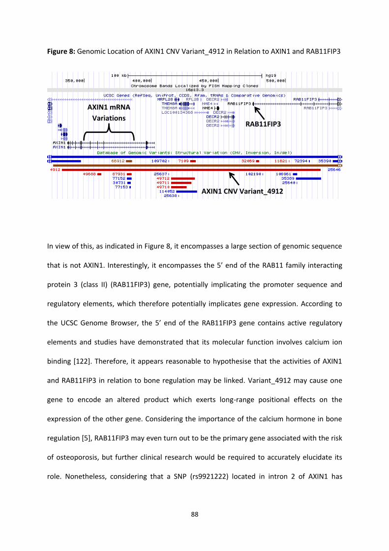
88

Figure 8: Genomic Location of AXIN1 CNV Variant_4912 in Relation to AXIN1 and RAB11FIP3

In view of this, as indicated in Figure 8, it encompasses a large section of genomic sequence

that is not AXIN1. Interestingly, it encompasses the 5’ end of the RAB11 family interacting

protein 3 (class II) (RAB11FIP3) gene, potentially implicating the promoter sequence and

regulatory elements, which therefore potentially implicates gene expression. According to

the UCSC Genome Browser, the 5’ end of the RAB11FIP3 gene contains active regulatory

elements and studies have demonstrated that its molecular function involves calcium ion

binding [122]. Therefore, it appears reasonable to hypothesise that the activities of AXIN1

and RAB11FIP3 in relation to bone regulation may be linked. Variant_4912 may cause one

gene to encode an altered product which exerts long-range positional effects on the

expression of the other gene. Considering the importance of the calcium hormone in bone

regulation [5], RAB11FIP3 may even turn out to be the primary gene associated with the risk

of osteoporosis, but further clinical research would be required to accurately elucidate its

role. Nonetheless, considering that a SNP (rs9921222) located in intron 2 of AXIN1 has

RAB11FIP3

AXIN1 CNV Variant_4912

AXIN1 mRNA

Variations

89

already been implicated in bone regulation, Variant_4912 seemed an appropriate CNV for

investigating the potential association between AXIN1 CNV and osteoporosis.

90

4.2 Materials and Methods

This study investigated the potential effect of two different CNVs on BMD, and although the

CNVs were analysed separately, all methods were applied in exactly the same manner,


CNV are collectively described in a general methods section (Refer to Chapter 2: Materials

and Methods).

91

4.3 Results

4.3.1 Quality Control

The first measure of quality control of the experimental data was that no TaqMan signals

were detected for DNA amplification in the NTC wells of every 384-well qPCR reaction plate

run. qPCR data were examined for consistency and confidence between the two technical

replicates of every analysed sample using the mean, SD, and SE, of the FAM and VIC signal

intensities on the CT scale. By criteria modified for this study (Refer to Section 2.2.5.1),

normally distributed data were located less than 1.0 SD above or below the mean. The

majority of analysed samples had a SD below 1.0, so they were within the acceptable

threshold, and thus were approved for statistical analysis. Higher SD tended to correlate

with a higher degree of variability displayed by the VIC signals, which were generally more

variable than the FAM signals. Several samples had a SD exceeding 1.0 and they were

defined as having an ‘unconfirmed’ CN (even if both technical replicates had the same CN

predicted by CopyCaller). ‘Unconfirmed’ samples were subjected to a second round of

genotyping, which in turn yielded an acceptable SD. Therefore, it was reasonably accepted

that the majority of qPCR data in this study were sufficiently reproducible and reliable for

CN assignment by CopyCaller.

CopyCaller results were then examined for consistency and confidence between the two

technical replicates of every analysed sample. By criteria modified for this study (Refer to

Section 2.2.5.1), a ‘confirmed’ CN was assigned to a sample if both replicates were assigned

the same CN and it also matched up with the CN yielded when replicate data were

combined to represent a single sample. Although CopyCaller could not produce a

confidence score for only two replicates, the proven reproducibility of the qPCR data

92

validated the reliability of the CopyCaller results. Moreover, the ‘confirmed’ CN for 9

subjects could be accurately validated based on consistency with their random biological

replicate included in the sample set. From the first round of genotyping, 441 out of 623

samples had both replicates assigned the same CN by CopyCaller with sufficient confidence,

and were thus defined as having a ‘confirmed’ CN and approved for statistical analysis. The

remaining 182 samples had a discrepancy in CN between their replicates. AXIN1 CNV

reagents were limiting at this point, so samples had to be prioritised for the second round of

genotyping based on certain criteria (Refer to Section 2.2.5.2). As a result, 78 samples which

had yielded an ‘undetermined’ CN for either replicate from the first round of genotyping

were completely eliminated from further analysis. Moreover, another 2 samples were

omitted due to insufficient stock volumes of gDNA. Therefore, 104 samples could be

analysed by qPCR and CopyCaller again.

From the second round of genotyping, 48 out of the 104 prioritised, previously

‘unconfirmed’ samples went on to yield a ‘confirmed’ CN with sufficient confidence.

However, the remaining 56 samples had failed, yet again, to yield a consistent CN between

all four replicates that had been analysed to date. By criteria modified for this study (Refer

to Section 2.2.5.3), a ‘confirmed’ CN was assigned to a sample if the CN call predicted by

CopyCaller, when replicate data were combined to represent a single sample, had a

confidence score greater than 7.0. From here, 31 further samples were assigned a

‘confirmed’ CN, yet 25 ‘unconfirmed’ samples with a poor confidence score still remained.

Considering that a third round of genotyping was unfeasible at this point due to limiting

reagents and time constraints, it was conceded that these samples had failed their reactions

and they were therefore completely eliminated from statistical analysis.

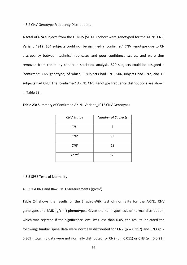
93

4.3.2 CNV Genotype Frequency Distributions

A total of 624 subjects from the GENOS (STH-H) cohort were genotyped for the AXIN1 CNV,

Variant_4912. 104 subjects could not be assigned a ‘confirmed’ CNV genotype due to CN

discrepancy between technical replicates and poor confidence scores, and were thus

removed from the study cohort in statistical analysis. 520 subjects could be assigned a

‘confirmed’ CNV genotype; of which, 1 subjects had CN1, 506 subjects had CN2, and 13

subjects had CN3. The ‘confirmed’ AXIN1 CNV genotype frequency distributions are shown

in Table 23.

Table 23: Summary of Confirmed AXIN1 Variant_4912 CNV Genotypes

CNV Status Number of Subjects

CN1 1

CN2 506

CN3 13

Total 520

4.3.3 SPSS Tests of Normality

4.3.3.1 AXIN1 and Raw BMD Measurements (g/cm2)

Table 24 shows the results of the Shapiro-Wilk test of normality for the AXIN1 CNV

genotypes and BMD (g/cm2) phenotypes. Given the null hypothesis of normal distribution,

which was rejected if the significance level was less than 0.05, the results indicated the

following; lumbar spine data were normally distributed for CN2 (p = 0.112) and CN3 (p =

0.309); total hip data were not normally distributed for CN2 (p = 0.011) or CN3 (p = 0.0.21);

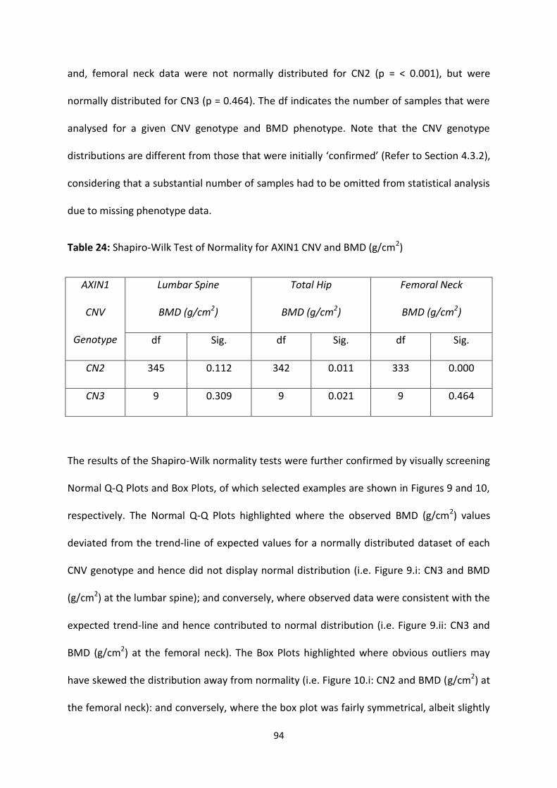
94

and, femoral neck data were not normally distributed for CN2 (p = < 0.001), but were

normally distributed for CN3 (p = 0.464). The df indicates the number of samples that were

analysed for a given CNV genotype and BMD phenotype. Note that the CNV genotype

distributions are different from those that were initially ‘confirmed’ (Refer to Section 4.3.2),

considering that a substantial number of samples had to be omitted from statistical analysis

due to missing phenotype data.

Table 24: Shapiro-Wilk Test of Normality for AXIN1 CNV and BMD (g/cm2)

AXIN1

CNV

Genotype

Lumbar Spine

BMD (g/cm2)

Total Hip

BMD (g/cm2)

Femoral Neck

BMD (g/cm2)


CN2 345 0.112 342 0.011 333 0.000

CN3 9 0.309 9 0.021 9 0.464



respectively. The Normal Q-Q Plots highlighted where the observed BMD (g/cm2) values

deviated from the trend-line of expected values for a normally distributed dataset of each

CNV genotype and hence did not display normal distribution (i.e. Figure 9.i: CN3 and BMD

(g/cm2) at the lumbar spine); and conversely, where observed data were consistent with the

expected trend-line and hence contributed to normal distribution (i.e. Figure 9.ii: CN3 and

BMD (g/cm2) at the femoral neck). The Box Plots highlighted where obvious outliers may

have skewed the distribution away from normality (i.e. Figure 10.i: CN2 and BMD (g/cm2) at

the femoral neck): and conversely, where the box plot was fairly symmetrical, albeit slightly

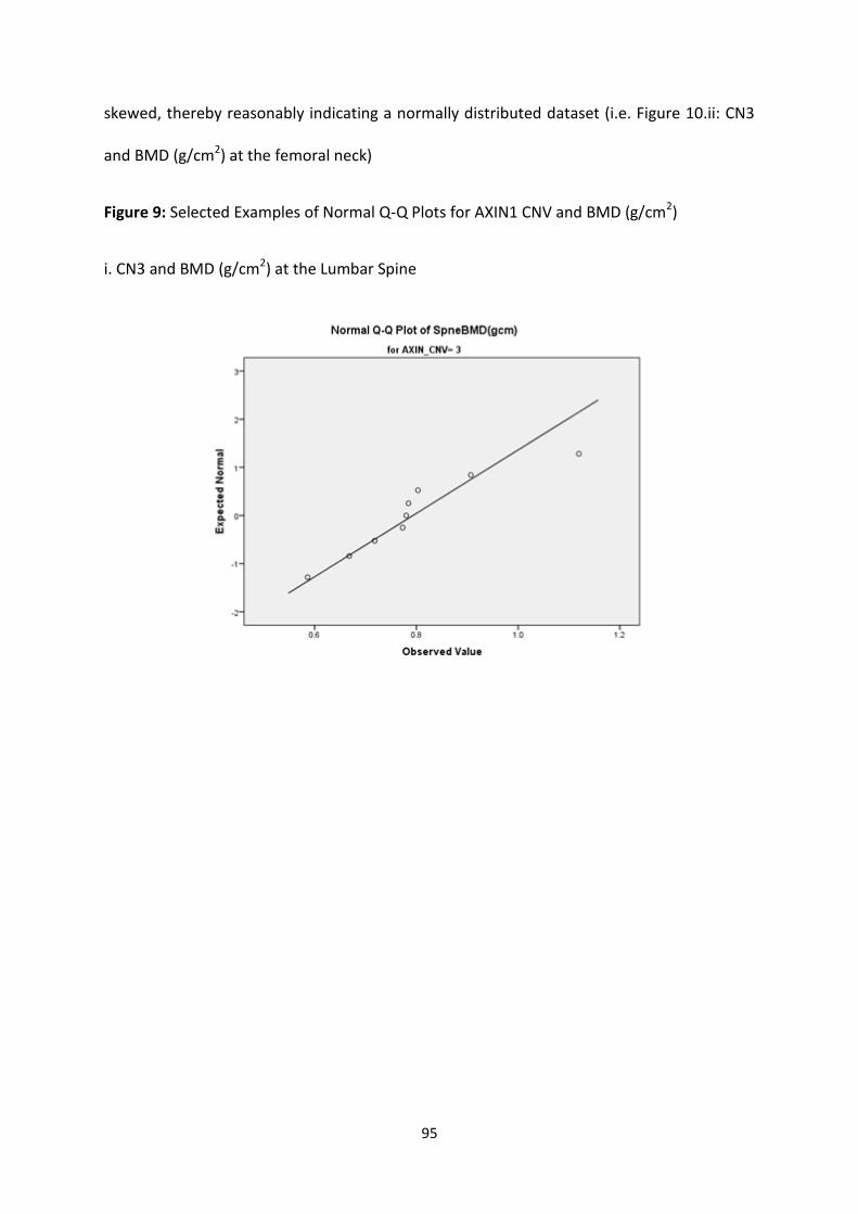
95

skewed, thereby reasonably indicating a normally distributed dataset (i.e. Figure 10.ii: CN3

and BMD (g/cm2) at the femoral neck)

Figure 9: Selected Examples of Normal Q-Q Plots for AXIN1 CNV and BMD (g/cm2)

i. CN3 and BMD (g/cm2) at the Lumbar Spine

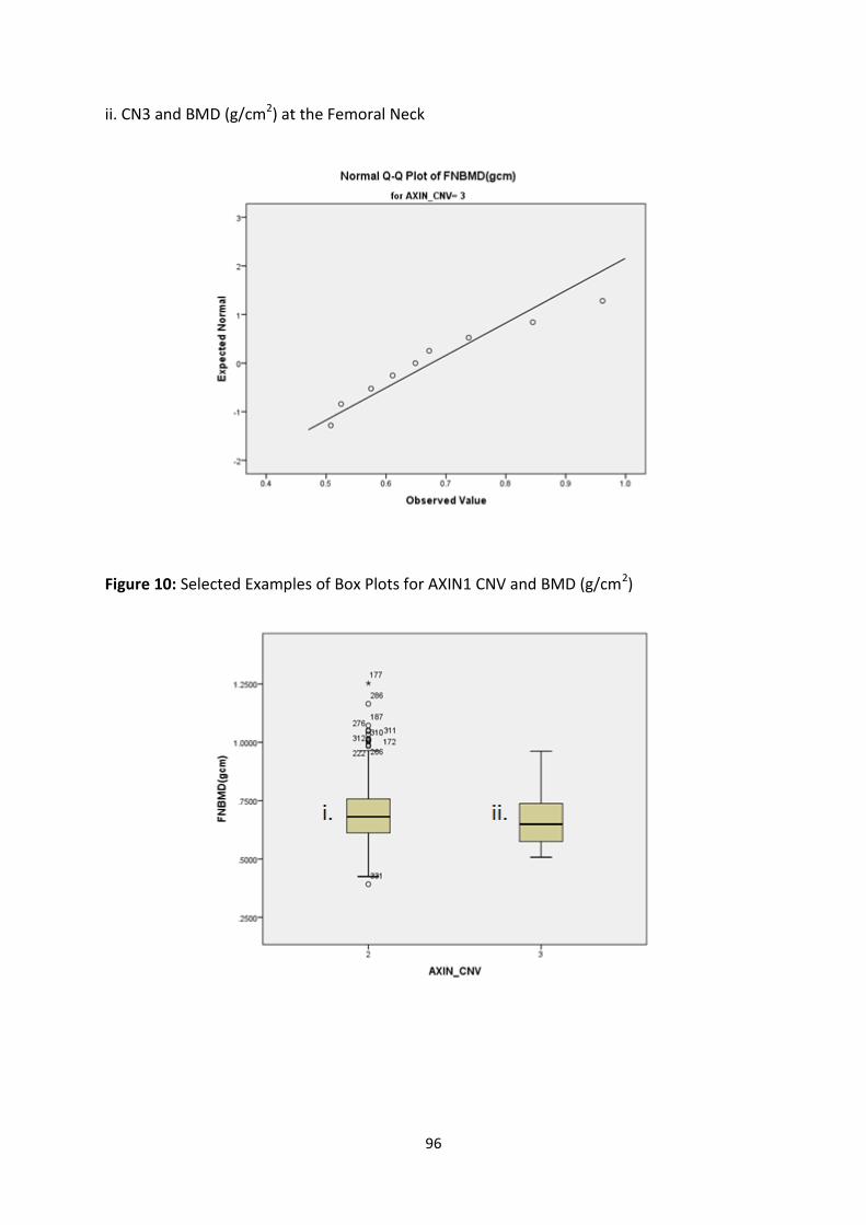
96

ii. CN3 and BMD (g/cm2) at the Femoral Neck

Figure 10: Selected Examples of Box Plots for AXIN1 CNV and BMD (g/cm2)

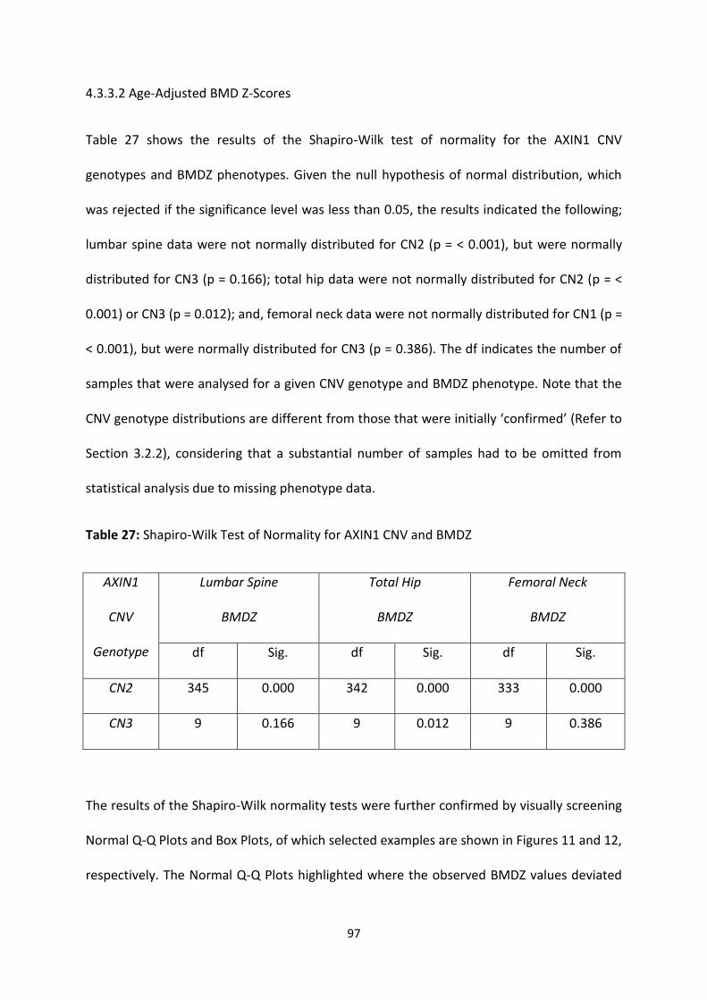
97

4.3.3.2 Age-Adjusted BMD Z-Scores

Table 27 shows the results of the Shapiro-Wilk test of normality for the AXIN1 CNV

genotypes and BMDZ phenotypes. Given the null hypothesis of normal distribution, which

was rejected if the significance level was less than 0.05, the results indicated the following;

lumbar spine data were not normally distributed for CN2 (p = < 0.001), but were normally

distributed for CN3 (p = 0.166); total hip data were not normally distributed for CN2 (p = <

0.001) or CN3 (p = 0.012); and, femoral neck data were not normally distributed for CN1 (p =

< 0.001), but were normally distributed for CN3 (p = 0.386). The df indicates the number of

samples that were analysed for a given CNV genotype and BMDZ phenotype. Note that the

CNV genotype distributions are different from those that were initially ‘confirmed’ (Refer to

Section 3.2.2), considering that a substantial number of samples had to be omitted from

statistical analysis due to missing phenotype data.

Table 27: Shapiro-Wilk Test of Normality for AXIN1 CNV and BMDZ

AXIN1

CNV

Genotype

Lumbar Spine

BMDZ

Total Hip

BMDZ

Femoral Neck

BMDZ


CN2 345 0.000 342 0.000 333 0.000

CN3 9 0.166 9 0.012 9 0.386



respectively. The Normal Q-Q Plots highlighted where the observed BMDZ values deviated

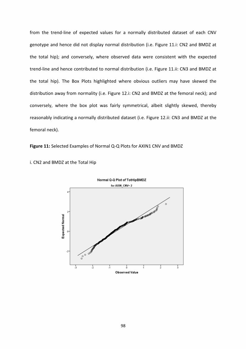
98

from the trend-line of expected values for a normally distributed dataset of each CNV

genotype and hence did not display normal distribution (i.e. Figure 11.i: CN2 and BMDZ at

the total hip); and conversely, where observed data were consistent with the expected

trend-line and hence contributed to normal distribution (i.e. Figure 11.ii: CN3 and BMDZ at

the total hip). The Box Plots highlighted where obvious outliers may have skewed the

distribution away from normality (i.e. Figure 12.i: CN2 and BMDZ at the femoral neck); and

conversely, where the box plot was fairly symmetrical, albeit slightly skewed, thereby

reasonably indicating a normally distributed dataset (i.e. Figure 12.ii: CN3 and BMDZ at the

femoral neck).

Figure 11: Selected Examples of Normal Q-Q Plots for AXIN1 CNV and BMDZ

i. CN2 and BMDZ at the Total Hip

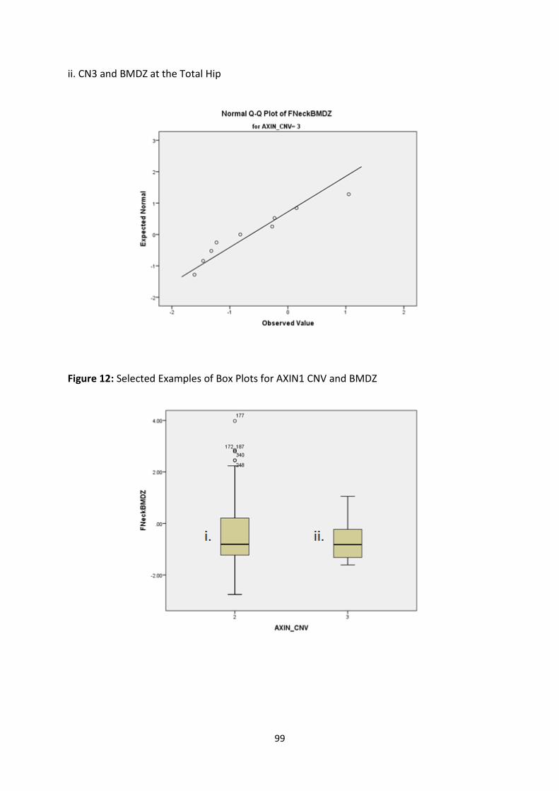
99

ii. CN3 and BMDZ at the Total Hip

Figure 12: Selected Examples of Box Plots for AXIN1 CNV and BMDZ

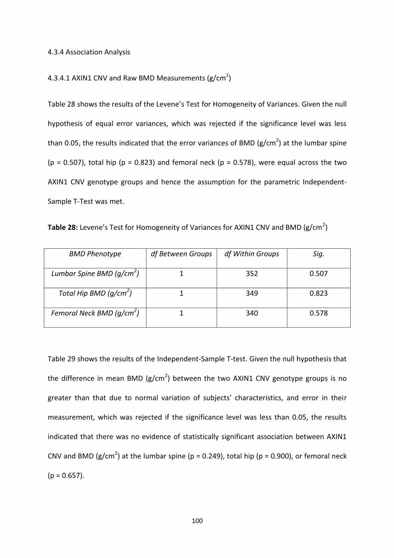
100

4.3.4 Association Analysis

4.3.4.1 AXIN1 CNV and Raw BMD Measurements (g/cm2)




(p = 0.507), total hip (p = 0.823) and femoral neck (p = 0.578), were equal across the two

AXIN1 CNV genotype groups and hence the assumption for the parametric Independent-

Sample T-Test was met.

Table 28: Levene’s Test for Homogeneity of Variances for AXIN1 CNV and BMD (g/cm2)





Table 29 shows the results of the Independent-Sample T-test. Given the null hypothesis that

the difference in mean BMD (g/cm2) between the two AXIN1 CNV genotype groups is no

greater than that due to normal variation of subjects’ characteristics, and error in their

measurement, which was rejected if the significance level was less than 0.05, the results

indicated that there was no evidence of statistically significant association between AXIN1

CNV and BMD (g/cm2) at the lumbar spine (p = 0.249), total hip (p = 0.900), or femoral neck

(p = 0.657).

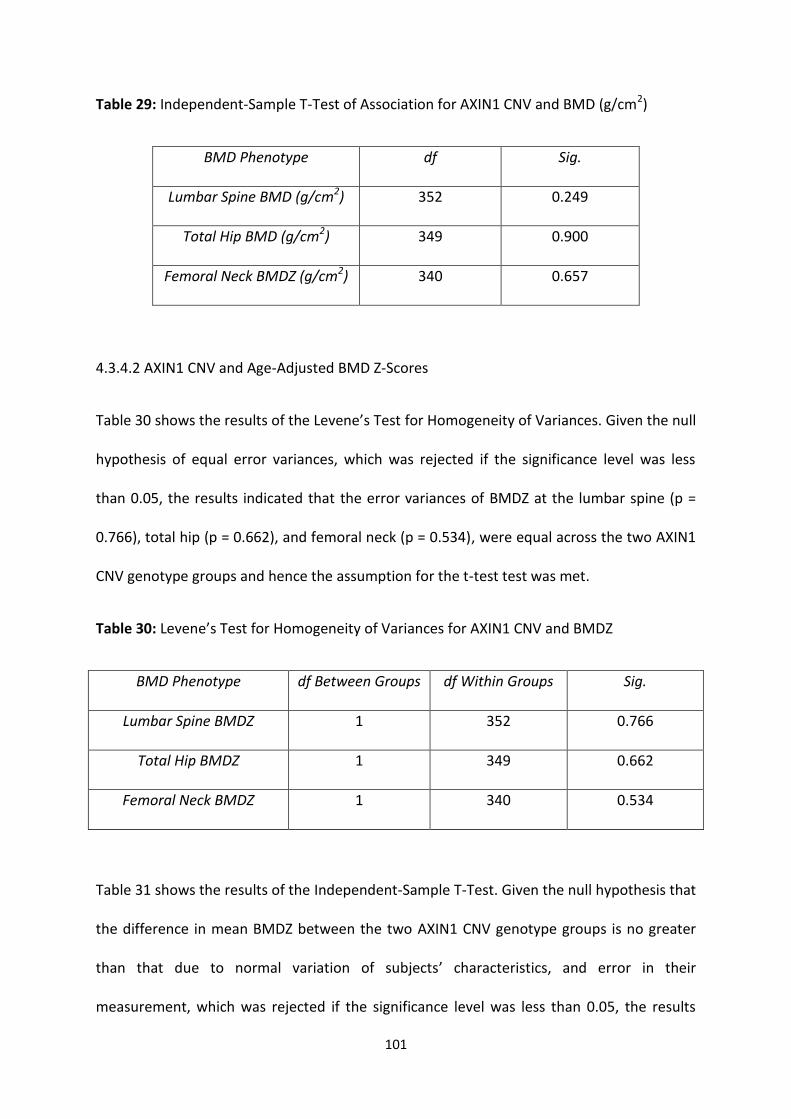
101

Table 29: Independent-Sample T-Test of Association for AXIN1 CNV and BMD (g/cm2)

BMD Phenotype df Sig.

Lumbar Spine BMD (g/cm2) 352 0.249

Total Hip BMD (g/cm2) 349 0.900

Femoral Neck BMDZ (g/cm2) 340 0.657

4.3.4.2 AXIN1 CNV and Age-Adjusted BMD Z-Scores



than 0.05, the results indicated that the error variances of BMDZ at the lumbar spine (p =

0.766), total hip (p = 0.662), and femoral neck (p = 0.534), were equal across the two AXIN1

CNV genotype groups and hence the assumption for the t-test test was met.

Table 30: Levene’s Test for Homogeneity of Variances for AXIN1 CNV and BMDZ





Table 31 shows the results of the Independent-Sample T-Test. Given the null hypothesis that

the difference in mean BMDZ between the two AXIN1 CNV genotype groups is no greater

than that due to normal variation of subjects’ characteristics, and error in their

measurement, which was rejected if the significance level was less than 0.05, the results

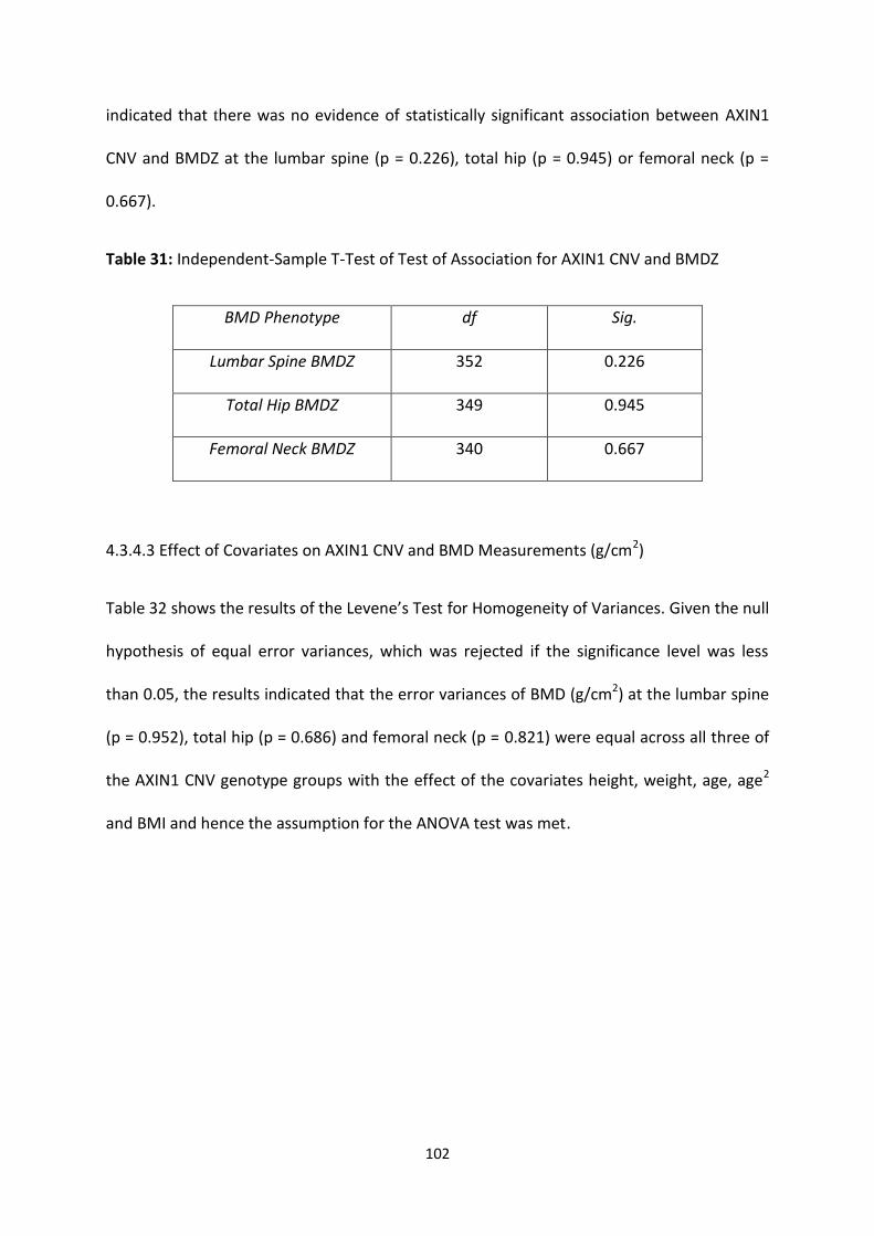
102

indicated that there was no evidence of statistically significant association between AXIN1

CNV and BMDZ at the lumbar spine (p = 0.226), total hip (p = 0.945) or femoral neck (p =

0.667).

Table 31: Independent-Sample T-Test of Test of Association for AXIN1 CNV and BMDZ

BMD Phenotype df Sig.

Lumbar Spine BMDZ 352 0.226

Total Hip BMDZ 349 0.945

Femoral Neck BMDZ 340 0.667

4.3.4.3 Effect of Covariates on AXIN1 CNV and BMD Measurements (g/cm2)




(p = 0.952), total hip (p = 0.686) and femoral neck (p = 0.821) were equal across all three of

the AXIN1 CNV genotype groups with the effect of the covariates height, weight, age, age2

and BMI and hence the assumption for the ANOVA test was met.

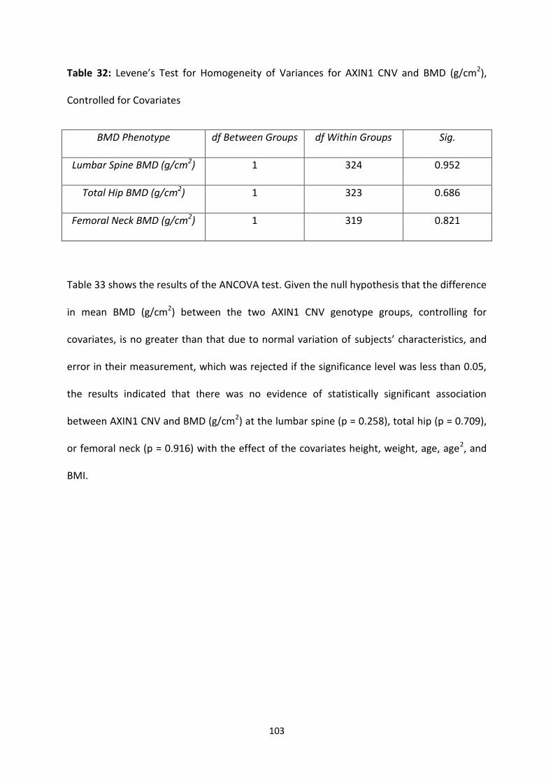
103

Table 32: Levene’s Test for Homogeneity of Variances for AXIN1 CNV and BMD (g/cm2),






Table 33 shows the results of the ANCOVA test. Given the null hypothesis that the difference

in mean BMD (g/cm2) between the two AXIN1 CNV genotype groups, controlling for

covariates, is no greater than that due to normal variation of subjects’ characteristics, and

error in their measurement, which was rejected if the significance level was less than 0.05,

the results indicated that there was no evidence of statistically significant association

between AXIN1 CNV and BMD (g/cm2) at the lumbar spine (p = 0.258), total hip (p = 0.709),

or femoral neck (p = 0.916) with the effect of the covariates height, weight, age, age2, and

BMI.

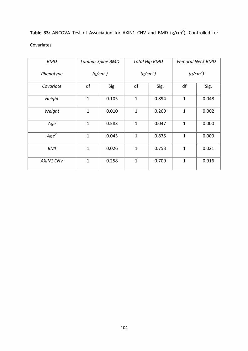
104

Table 33: ANCOVA Test of Association for AXIN1 CNV and BMD (g/cm2), Controlled for

Covariates

BMD

Phenotype

Lumbar Spine BMD

(g/cm2)

Total Hip BMD

(g/cm2)

Femoral Neck BMD

(g/cm2)

Covariate df Sig. df Sig. df Sig.

Height 1 0.105 1 0.894 1 0.048

Weight 1 0.010 1 0.269 1 0.002

Age 1 0.583 1 0.047 1 0.000

Age2 1 0.043 1 0.875 1 0.009

BMI 1 0.026 1 0.753 1 0.021

AXIN1 CNV 1 0.258 1 0.709 1 0.916

105

4.4 Discussion

This study investigated the potential effect of CNV in the pathogenesis of osteoporosis, with

a CNV of the AXIN1 gene being one of the two CNVs of interest. The AXIN1 gene encoding

the Axin-1 protein and inhibiting the Wnt signalling pathway is a recognised candidate for

the genetic regulation of phenotypes related to the risk of osteoporosis, such as BMD, bone

mass, and bone remodelling. In previous studies, a SNP (rs9921222) located in intron 2 of

AXIN1 has been described and its associations with BMD have been reported, but the exact

functional role of AXIN1 and hence the consequence of AXIN1 CNV has yet to be fully

elucidated. Nonetheless, there is still evidence supporting the association between genetic

variation of AXIN1 and the surrogate phenotype of osteoporosis, BMD.

The presence of AXIN1 CNV in the analysed cohort was indicated by the observation of

three distinct CNV genotype groups, representing CN loss (CN1) and CN gain (CN3) from the

expected wild-type CN in the human diploid genome (CN2). The discovery study that

originally detected the AXIN1 CNV Variant_4912 reported that it constitutes a loss in AXIN1

CN [131]. The only subject confirmed for the presence of CN loss in this current study had to

be omitted from statistical analysis due to missing phenotype data. Therefore, the effect of

AXIN1 CNV in terms of the specific CNV Variant_4912 could not be statistically analysed.

Nonetheless, two other CNV genotype groups were sufficiently represented in statistical

analysis; CN gain (CN3) from the expected wild-type CN in the human diploid genome (CN2).

In general, CNVs are thought to have quantitative effects, so CN loss or gain may equally

affect a given trait. Moreover, evidence suggests the possibility of allelic heterogeneity at

given genetic loci among different populations [142]. In view of this, even though the CN1

genotype for AXIN1 CNV was not represented, the CN3 genotype could still be statistically

106

analysed. Therefore, this study tested the potential effect of the AXIN1 CNV in relation to

BMD at three common skeletal locations of osteoporotic fracture (i.e. lumbar spine, total

hip, and femoral neck) in a family-based population cohort study of Caucasian women from

Australia and the UK. This study did not detect any statistically significant associations

between AXIN1 CNV and BMD (g/cm2) at the lumbar spine, total hip, or femoral neck, in the

analysed subject cohort. Moreover, no associations were found between AXIN1 CNV and

BMD after the BMD data were corrected for age (BMDZ) at the three skeletal locations in

the cohort. Furthermore, no associations were found after testing the potential effect of

covariates (i.e. age, age2, height, weight, and BMI) on the relationship between AXIN1 CNV

and BMD (g/cm2) at the three skeletal locations in the cohort. Therefore, in this study of

Caucasian women, the AXIN1 CNV genotype had no statistically significant effect on the

BMD phenotype. However, this study was specifically designed to target, amplify, and

detect, Variant_4912, which constitutes a CN loss (CN1) from the expected wild-type (CN2).

Therefore, the modified interpretation of AXIN1 CNV based on the two CNV genotypes that

were observed (i.e. CN2 and CN3) is not fully comprehensive. The relatively poor CNV

genotype coverage achieved in this study was potentially due to poor specificity of the

TaqMan Assays in terms of annealing and amplification, but further research would be

required to accurately elucidate this.

In summary, this study successfully genotyped AXIN1 CNV and tested for its potential

association with BMD, but found no statistically significant association. Previous studies

have indicated that the AXIN1 gene inhibits the Wnt signalling pathway [135; 136] and it has

been demonstrated that Wnt signal transduction protects against phenotypes related to

osteoporosis, such as low BMD [19]. Moreover, previous studies have implicated an AXIN1

107

SNP with BMD [133]. Interestingly, previous studies have shown that AXIN1 negatively

regulates the canonical Wnt signalling pathway by inhibiting the degradation of β-catenin

[135; 136]. Moreover, β-catenin overexpression has been shown to reduce the promoter

activity of RANKL [139]. Therefore, considering that RANKL activates osteoclasts and

promotes bone loss [18], a loss-of-function mutation related to AXIN1 CNV Variant_4912

could potentially offer protection against phenotypes related to osteoporosis. Therefore,

AXIN1 CNV was anticipated to have a more significant effect on BMD than was found in this

study, but whether data from this study would be replicated in a very large population study

with sufficient statistical power, such as those used in recent GWAS meta-analyses (i.e. of

the order of 80,000 subjects) remains to be elucidated.

There have been no previous studies of the AXIN1 CNV Variant_4912 and hence its clinical

relevance to BMD or other phenotypes related to the risk of osteoporosis remains to be

elucidated. Therefore, it would be impossible to accurately validate or refute the findings

without any corroborating evidence from previous studies. Nonetheless, there is evidence

from previous studies implicating intron 2 of the AXIN1 gene with BMD. Variant_4912

encompasses the entirety of the AXIN1 gene, thereby implicating the transcriptional unit,

which implicates gene expression, the fundamental level at which the genotype gives rise to

the phenotype [67]. Therefore, despite the lack of statistically significant findings in this

study, the AXIN1 CNV Variant_4912 still remains a promising candidate for involvement in

BMD and the risk of osteoporosis.

108

Chapter 5: General Discussion and Conclusion

109

5.1 General Discussion

Given what was already known about osteoporosis, gene expression, and CNV, the general

purpose of this study was to investigate whether CNV of genomic regions, whose wild-type

expression has previously been implicated with the regulation of bone, has an influence on

the regulation of the surrogate phenotype for osteoporosis, BMD, and thus whether it

influences the risk of developing the disease.

Therefore, in an attempt to better elucidate the potential relationship between CNV and

osteoporosis for further research, the main aim of this study was to examine the potential

effect of two novel CNVs of the genes ESR1 and AXIN1, Variant_4512 and Variant_4912,

respectively, in relation to BMD, in a population cohort study of Caucasian women.

Furthermore, the specific aims, with which the main aim was addressed, were as follows;

1) To attempt the accurate detection and quantitation of Variant_4512 and Variant_4912,

respectively, in every subject of the study cohort, using relatively novel CNV genotyping

techniques via qPCR combined with TaqMan chemistries, and the CN quantitation software,

CopyCaller.

2) To examine the potential effect of Variant_4512 and Variant_4912, respectively, in the

study cohort, in relation to three different BMD phenotypes: 1) raw measurement (g/cm2),

2) age-adjusted Z-score, and 3) controlled for several covariates, at three common skeletal

locations of osteoporotic fracture: 1) the lumbar spine, 2) total hip, and 3) femoral neck,

using analyses of variance via the statistics software, SPSS.

110

5.1.1 CNV Detection and Quantitation

Based on the experimental results obtained from the CNV genotyping component of this

study, there are several interpretations which can be made for the analyses of ESR1 CNV

and AXIN1 CNV.

Firstly, experimental data from both CNV analyses were validated as reproducible and

reliable. No DNA amplification occurred in the NTC wells of every qPCR reaction plate run,

thereby confirming that contamination of experimental reagents was successfully avoided.

All data from qPCR and CopyCaller were reasonably consistent between replicates with

acceptable confidence levels. However, the VIC signal intensities on the CT scale tended to

be more variable when compared with those of FAM. This may have been due to a higher

degree of sensitivity and discrimination displayed by the TaqMan CN Reference Assays, but

further research would be required to accurately validate this. The SPSS tests of normality

(i.e. Shapiro-Wilk, Q-Q Plots and Box Plots) were largely inconsistent for both CNV analyses,

with varying degrees of normality depending on the CNV status and BMD phenotype (i.e.

data and location). Nonetheless, the majority of data tended slightly more towards normal

distribution. Data lacking normality were most likely influenced by a lack of statistical power

in this study due to an insufficient dataset from a moderately sized subject cohort, having

many subjects that could not be statistically analysed due to missing phenotype data.

Nonetheless, since the majority of data displayed normal distribution, it was reasonably

assumed that association analyses could be performed using parametric tests via SPSS.

Secondly, the genotype distributions observed among the cohort study revealed the

presence of both ESR1 CNV and AXIN1 CNV. This was indicated by the detection of

infrequent loss (CN1) and gain (CN3) from the expected human diploid wild-type CN for

111

both genes (CN2). Interestingly, the observed genotypes of CN loss for ESR1 (CN1) and CN

gain for AXIN1 (CN3) were not expected, considering Variant_4512 constitutes a CN gain for

ESR1 (CN3) and Variant_4912 constitutes a CN loss for AXIN1 (CN1). Whilst the exact

reasoning for this is unclear, there are several possible explanations, including poor

specificity of the pre-designed TaqMan CN Assays in terms of annealing and amplification of

the genomic region of interest, or inaccurate CN quantitation by CopyCaller from using only

two technical replicates for each sample instead of the four that is recommended by ABI.

Although experimental error and inconsistencies would appear to have the most obvious

contribution towards the unexpected results, there might be some confounding feature

about the CNVs that has not yet been elucidated. For example, the three observed CNV

genotypes for both genes might be a result of allelic heterogeneity at their respective loci

among different populations [111]. Further research would be required to comprehensively

elucidate whether the observed CNV genotypes were in fact accurate, but due to limiting

reagents and time constraints it was not feasible in this study.

Another observation from the genotyping results in this study was that the frequencies of

Variant_4512 and Variant_4912 were not the same as those reported by Wong et al in 2007

in the discovery study for CNV detection. Instead, Variant_4512 and Variant_4912 were

detected at frequencies of 0.99% and 0.2% in this study, which is significantly lower than the

frequencies of 21% and 20% reported in the discovery study. The inconsistencies in CNV

frequencies between this current study and the discovery study were most likely due to the

differences in experimental conditions. The two subject cohorts were not representative of

each other in terms of the distributions of subjects’ characteristics. This current study

consisted exclusively of Caucasian women, while the discovery study consisted of both

112

women and men from a range of different ethnicities. This further highlights the possibility

of allelic heterogeneity among different populations. The two methods of CNV detection

were also different. This current study used qPCR combined with TaqMan Assay chemistries,

while the discovery study used BAC array CGH analysis. Although experimental differences

appear to be the most obvious reason as to why there was discrepancy in CNV frequencies

between the two studies, the low frequencies observed in this study might ultimately signify

that Variant_4512 and Variant_4912 are rare variants within the specific population cohort

of Caucasian women from Australia and the UK. However, further research would be

required to accurately elucidate this. Previous studies have suggested that rare variants may

be as important as common variants in complex traits and diseases such as osteoporosis

[50], but it is currently difficult to reliably detect the effects of rare variants given the

constraints associated with sample size and sequencing [43].

Thirdly, in hindsight, the pre-designed TaqMan CN Assay used to detect the ESR1 CNV

Variant_4512 appeared to have been poorly selected for this study. It was intended to

target the middle of Variant_4512, so as to ensure adequate coverage of the genomic

region in terms of both annealing and amplification specificity. As a result, the CN Assay

targeted a region in intron 2 of the ESR1 gene and subsequently amplified a genomic

sequence 88 bp in length [112]. However, a target location in intron 1 of ESR1 would have

been more appropriate for this study, considering that previous studies have implicated

genetic variations within intron 1 and the 5’ end of ESR1 with BMD [49; 98]. Moreover, a

target location upstream of ESR1 and not overlapping any other coding regions may have

also been appropriate, considering that previous studies have acknowledged the majority of

known genes subject to CNV are not even located within the identified region of genetic

113

variation [84], and that osteoporosis might be more susceptible to genetic variation

affecting the CN of non-coding DNA sequences [89]. The pre-designed TaqMan CN Assay

used to detect the AXIN1 CNV Variant_4912 had initially seemed appropriately selected for

this study. Again, it was selected to target the middle of Variant_4912, so as to ensure

adequate coverage of the genomic region in terms of both annealing and amplification

specificity. As a result, the CN Assay targeted a region in exon 3 of the AXIN1 gene and

subsequently amplified a genomic sequence 110 bp in length [112]. However, this study

detected Variant_4912 in only one subject, who could not be statistically analysed due to

missing phenotype data. However, even if this CNV genotype for the one subject was

represented in statistical analysis, the statistical power would have been so low that there

would have been minimal chance of yielding a significant result. Considering that previous

studies have implicated a SNP (rs9921222) in intron 2 of AXIN1 with BMD [133],

Variant_4912 was anticipated to have a more significant effect on BMD. Nonetheless, this

study confirmed the presence of both ESR1 CNV and AXIN1 CNV in the analysed subject

cohort, as indicated by the observation of three distinct CNV genotypes for each gene,

representing CN loss (CN1) and CN gain (CN3) from the expected wild-type CN, most

frequent in the human diploid genome (CN2).

5.1.2 CNV Association with BMD

In summary, whilst the association analyses were successfully conducted and appropriately

interpreted, the findings in this study illustrated a comprehensive lack of association

between BMD and CNV of both ESR1 and AXIN1, which was not consistent with what was

initially hypothesised, based on what is already known about the two genes.

114

When considering the analysis of ESR1 CNV, Variant_4512 was anticipated to have a more

significant effect on BMD than was found in this study. Previous studies have indicated that

the ESR1 gene mediates the response of target cells to oestrogen, which has been

demonstrated to protect against phenotypes related to osteoporosis, such as low BMD.

Moreover, previous studies have implicated several genetic variations of ESR1 with BMD.

Nonetheless, results have been largely inconsistent between studies for statistical reasons,

such as lack of power and study design [49], and more recently, it has been suggested that

there could be allelic heterogeneity at the ESR1 locus among different populations [142].

Therefore, despite there being no evidence of association between ESR1 CNV and BMD in

this study, given different experimental conditions, such as a larger sample size with a

related increase in statistical power, a statistically significant association may have been

identified. Nonetheless, an interesting observation of this study was that the effect of ESR1

CNV in relation to BMD (g/cm2) at the femoral neck increased dramatically, and was noted

as nominally significant, when controlled for several covariates (p = 0.052). It appears that

this near-significant association was influenced by the extremely statistically significant

associations between BMD (g/cm2) at the femoral neck, and age (p = < 0.001) and weight (p

= 0.009). This finding was particularly meaningful for this study, considering what is already

understood about both osteoporosis and CNV. Being a common complex disease,

osteoporosis involves interactions among multiple risk factors of both genetic and

environmental sources [42]. Moreover, functional CNVs are anticipated to encompass

‘environmental sensor’ genes that are not critical for development, but mediate interaction

with the environment [84]. Therefore, this could potentially explain how Variant_4512 could

be present within the genome of an otherwise healthy person and not directly cause

osteoporosis, but instead contribute to an enhanced susceptibility (i.e. influence low BMD at

115

the femoral neck) given exposure to specific environmental factors (i.e. the stable factor of

age and the modifiable factor of weight). Furthermore, Variant_4512 starts upstream of

ESR1 in a genomic region of currently unknown expression and function, which may even

turn out to be an ‘environmental sensor’ gene that influences BMD and osteoporosis risk.

However, these are hypothetical interpretations that would require further research to

accurately elucidate.

When considering the analysis of AXIN1 CNV, the specific CNV Variant_4912 may not have

been represented in statistical analysis, but the CNV genotype group CN3 was successfully

analysed. However, this modified interpretation of AXIN1 CNV was anticipated to have a

more significant effect on BMD than was found in this study. Previous studies have indicated

that the AXIN1 gene inhibits the Wnt signalling pathway [135; 136] and that Wnt proteins

protect against phenotypes related to osteoporosis, such as low BMD [19]. Moreover,

previous studies have implicated a genetic variation of AXIN1 with BMD [133]. Repeating

the experiments would have been beneficial towards validating the observed AXIN1 CNV

genotypes, but due to limiting reagents and time constraints, it was unfeasible in this study.

5.1.3 Recommendations for Further Study

Due to a combination of numerous technical issues, limiting reagents, and time constraints,

the general purpose of this study was not as comprehensively addressed as first intended.

Nonetheless, this study cemented a preliminary foundation, based on important concepts

and novel technologies, upon which future studies can build. Specifically, CNV assays for

two key genes related to BMD were effectively established in the laboratory and the study

cohort was successfully genotyped. Moreover, a protocol for the statistical approach for

analysis of genotyped data from de novo CNV assays was also established. There are several

116

recommendations for further study of the potential effect of ESR1 CNV and AXIN1 CNV in

relation to BMD and the risk of osteoporosis. Firstly, it would be beneficial to select a

subject cohort of the largest possible size and to ensure that clinical phenotype data is

recorded and stored appropriately for every subject, so as to ensure sufficient statistical

power and to increase the chance of yielding a significant association [116]. Secondly, if the

selected subject cohort is a family-based population, it would be beneficial to perform a

family-based population analysis. In family-based studies, using computer software

programs such as FBLAT and PLINK [142], genetic association of traits are assessed within

families and hence the confounding effect of population heterogeneity can be eliminated

[142]. Despite the fact that the GENOS (STH-S) cohort consists of twins and siblings and that

BMD is a highly heritable trait, a family-based association analysis was deemed unnecessary

for this current study, because none of the individuals with the ESR1 CNV Variant_4512

were related. Lastly, it would be beneficial to also undertake cell-based expression studies

to verify the normal activity of ESR1 and AXIN1 in regards to the regulation of bone, and the

functional effect of their respective CNVs. Moreover, the identification of biochemical

markers of phenotypes related to osteoporosis (i.e. excessive bone resorption) might just

implicate the functional consequence of CNV with the pathogenesis of osteoporosis,

thereby validating a new target for therapeutic intervention with the likelihood of

dramatically improving the quality of life for affected individuals.

117

5.2 Conclusion

This study tested the hypothesis that CNV is associated with BMD by investigating the

potential effect of two novel CNVs of genes, ESR1 and AXIN1, which have already been

implicated with the regulation of bone, in relation to BMD measurements at multiple

skeletal locations in a population study cohort of Caucasian women, between the ages of 18

and 83, from Australia and the UK.

Overall, this study effectively established CNV assays in the laboratory for two key genes

related to BMD, and the study cohort was successfully genotyped. Moreover, a protocol for

the statistical approach for analysis of genotyped data from the de novo CNV assays was

also successfully established. However, this study failed to demonstrate evidence of a

statistically significant association between CNV and BMD and therefore the hypothesis is

not supported.

In specific summary, in a study of Caucasian women, both ESR1 CNV and AXIN1 CNV were

accurately detected and quantitated using qPCR combined with TaqMan chemistries, and

the CN quantitation software, CopyCaller. Moreover, the potential effect of both CNVs in

relation to BMD was successfully examined using analyses of variance via the statistics

package, SPSS. However, it can be concluded that both CNVs have no clinically relevant

association with the regulation of BMD at multiple common skeletal locations of

osteoporotic fracture in the study cohort. Therefore, at this stage, both CNVs are unlikely to

play a major role in the pathogenesis of osteoporosis. However, further research would be

required to accurately validate this.

118

There have been no previous studies of the ESR1 CNV Variant_4512 or the AXIN1 CNV

Variant_4912 and hence their clinical relevance to BMD or other phenotypes related to the

risk of osteoporosis remains to be elucidated. Therefore, it would be impossible to

accurately validate the findings of this study without any corroborating evidence from

previous studies. Nonetheless, there is evidence from previous studies implicating intron 1

and the 5’ end of the ESR1 gene and intron 2 of the AXIN1 gene with BMD. Moreover,

Variant_4512 and Variant_4912 both encompass the 5’ end of their respective genes,

thereby implicating the promoter sequence and regulatory elements, which in turn

implicates the control of gene expression, which is the fundamental level at which the

genotype gives rise to the phenotype. Therefore, despite the lack of statistically significant

findings in this study, genomic CNVs of the genes ESR1 and AXIN1 still remain as promising

candidates for involvement in BMD and the risk of osteoporosis.

119

References

1. Woolf, A.D. and Pfleger, B. Burden of major musculoskeletal conditions. Bulletin of the

World Health Organization. 2003;81(9):646-656

2. Khurana, J.S. and Fitzpatrick, L.A. Osteoporosis and Metabolic Bone Disease. Bone

Pathology. 2009:217-237

3. Kastner, M., et al. Evaluation of a clinical decision support tool for osteoporosis

disease management: protocol for an interrupted time series design. Implementation

Science. 2011;6(77):1-7

4. Australian Institute of Health and Welfare. A snapshot of osteoporosis in Australia

2011. Canberra; 2011; Available from: http://aihw.gov.au

5. Raisz, L.G. Pathogenesis of osteoporosis: concepts, conflicts, and prospects. Journal of

Clinical Investigation. 2005;115(12):3318-3325

6. Brandi, M.L. Microarchitecture, the key to bone quality. Rheumatology. 2009;48:3-8

7. Cooper, C., et al. The epidemiology of vertebral fractures. Bone. 1993;14(1):89-97

8. Schütte, H.E., et al. Social and economic impact of osteoporosis. A review of the

literature. European Journal of Radiology. 1995;20(3):165-169

9. Osteoporosis Australia. About Osteoporosis. NSW; 2011; Available from:

http://osteoporosis.org.au

10. Lewiecki, E.M. Management of osteoporosis. Clinical and Molecular Allergy.

2004;2(9):1-11

11. Silverman, S. Quality-of-life issues in osteoporosis. Current Rheumatology Reports.

2005;7(1):39-45

12. Roche, J.J.W., et al. Effect of comorbidities and postoperative complications on

mortality after hip fracture in elderly people: prospective observational cohort study.

British Medical Journal. 2005;331(7529):1374-1379

13. Access Economics Pty Ltd. The Burden of Brittle Bones: Costing Osteoporosis in

Australia. Canberra; 2007; Available from: http://athritisvic.org.au

14. Walsh, M.C., et al. Osteoimmunology: Interplay Between the Immune System and

Bone Metabolism. Annual Review of Immunology. 2006;24:33-63

15. Clarke, B. Normal Bone Anatomy and Physiology. Journal of the American Society of

Nephrology. 2008;3:131-139

http://www.aihw.gov.au/

http://www.osteoporosis.org.au/

http://athritisvic.org.au/

120

16. Novak, D. and Faccio, R. Osteoclast motility: Putting the brakes on bone resorption.

Ageing Research Reviews. 2009;10(1):54-61

17. Sherwood, L. (2010) Human Physiology: From Cells to Systems. 7th Ed. Belmont;

Brooks/Cole Cengage Learning

18. Kearns, A.E., et al. Receptor Activator of Nuclear Factor ĸβ Ligand and Osteoprotegerin

Regulation of Bone Remodelling in Health and Disease. Endocrine Reviews.

2008;29(2):155-192

19. Ralston, S.H. and Uitterlinden, A.G. Genetics of Osteoporosis. Endocrine Reviews.

2010;31(5):1-34

20. Hofbauer, L.C. and Schoppet, M. Clinical Implications of the

Osteoprotegerin/RANKL/RANK System for Bone and Vascular Diseases. Journal of the

American Medical Association. 2004;292(4):490-495

21. Cohen, A.J. and Roe, F.J.C. Review of risk factors for osteoporosis with particular

reference to a possible aetiological role of dietary salt. Food and Chemical Toxicology.

2000;38(2-3):237-253

22. Bartl, R., Frisch, B., and Bartl, C. (2009) Osteoporosis: Diagnosis, Prevention and

Therapy. 2nd Ed. Berlin; Springer-Verlag

23. Clark, R. (2005) Anatomy and Physiology: Understanding the Human Body. London;

Jones & Bartlett Publishers

24. Al-Azzawi, F. and Palacios, S. Hormonal changes during menopause. Maturitas.

2009;63(2):135-137

25. Patel, R. and Lyles, K. (2009) Osteoporosis in Older Persons: Pathophysiology and

Therapeutic Approach. London; Springer-Verlag

26. Gueldner, S., Newman, E. and Grabo, T. (2008) Osteoporosis: Clinical Guidelines for

Prevention, Diagnosis and Management. New York; Springer Publishing Company

27. Manolagas, S.C. From Estrogen-Centric to Aging and Oxidative Stress: A Revised

Perception of the Pathogenesis of Osteoporosis. Endocrine Reviews. 2010;31(3):266-

300

28. Chen, Y., et al. Choice of study phenotype in osteoporosis genetic research. Journal of

Bone and Mineral Metabolism. 2009;27(2):121-126

121

29. Deng, H.W., et al. Determination of bone mineral density of the hip and spine in

human pedigrees by genetic and life-style factors. Genetic Epidemiology.

2000;19(2):160-177

30. Stephan, J. Techniques for measuring bone mineral density. International Congress

Series. 2002;1229:63-68

31. el Maghraoui, A. and Roux, C. DXA scanning in clinical practice. International Journal of

Medicine. 2008;101:605-617

32. National Institute of Health - Osteoporosis and Related Bone Diseases - National

Resource Centre. Bone Mass Measurement: What the Numbers Mean. Bethesda;

2009; Available from: http://bones.nih.gov

33. Saladin, K. (2004) Anatomy and Physiology: The Unity of Form and Function. 3rd Ed.

New York; McGraw-Hill

34. Sanders, K., et al. Calcium and bone health: Position statement for the Australian and

New Zealand Bone and Mineral Society, Osteoporosis Australia and the Endocrine

Society of Australia. Medical Journal of Australia. 2009;190(6);316-320

35. Bᴂksgaard, L., Andersen, K.P. and Hyldstrup, L. Calcium and Vitamin D

Supplementation Increases Spinal BMD in Healthy, Postmenopausal Women.

Osteoporosis International. 1998;8(3):255-260

36. Chan, K.M., Anderson, M. and Lau, E.M.C. Exercise interventions: defusing the world’s

osteoporosis time bomb. Bulletin of the World Health Organization. 2003;81(11):827-

830

37. Papapoulos, S. and O’Neill, T. Can we prevent fractures? Baillière’s Clinical

Rheumatology. 1997;11(3):565-582

38. Zaidi, M., et al. Osteoclastogenesis, Bone Resorption, and Osteoclast-Based

Therapeutics. Journal of Bone and Mineral Research. 2003;18(4):599-609

39. Delmas, P. Treatment of postmenopausal osteoporosis. Lancet. 2002;359:2018-2026

40. Ralston, S.H. and de Crombrugghe, B. Genetic regulation of bone mass and

susceptibility to osteoporosis. Genes & Development. 2006;20:2492-2506

41. Adeyemo, A., et al. Genetic variations associated with complex human diseases show

wide variation across multiple populations. Public Health Genomics. 2010;13:72-79

42. Yang, Q., et al. How many genes underlie the occurrence of common complex diseases

in the population? International Journal of Epidemiology. 2005;34(5):1129-1137

http://www.bones.nih.gov/

122

43. Lango, H., et al. What will whole genome searches for susceptibility genes for common

complex disease offer to clinical practice? Journal of Internal Medicine. 2008;263:16-

27

44. Manolio, T.A, et al. Finding the missing heritability of complex diseases. Nature.

2009;461:747-753

45. Laird, N.M. and Lange, C. (2011) Principles of inheritance: Mendel’s laws and genetic

models. Fundamentals of Modern Statistical Genetics. New York; Springer Science

46. Craig, J., et al. Complex diseases: research and applications. Nature. 2008;1(1);

Available from: http://nature.com

47. Cooper, R.S., et al. Gene-environment interactions and the etiology of common

complex disease. Annals of Internal Medicine. 2003;139(5):437-440

48. Kung, A.W.C. and Huang, Q-Y. Genetic and environmental determinants of

osteoporosis. Journal of Musculoskeletal and Neuronal Interactions. 2007;7(1):26-32

49. van Meurs, J.B.J., et al. Association of 5’ estrogen receptor alpha gene polymorphisms

with bone minder density, vertebral bone area and fracture risk. Human Molecular

Genetics. 2003;12(14):1745-1754

50. Pritchard, J.K., et al. The allelic architecture of human disease genes: common disease-

common variant…or not? Human Molecular Genetics. 2002;11(20):2417-2423

51. Zmulda, J.M., Cauley, J.A. and Ferrell, R.E. Recent progress in understanding the

genetic susceptibility to osteoporosis. Genetic Epidemiology. 1999;16(4):356-367

52. Newton-Cheh, C., et al. Genetic association studies of complex traits: design and

analysis issues. Mutation Research. 2005;573:54-69

53. Duncan, E. and Brown, M. Mapping genes for osteoporosis – old dogs and new tricks.

Bone. 2010;46:1219-1225

54. Pearson, T. and Manolio, T. How to Interpret a Genome-wide Association Study.

Journal of the American Medical Association. 2008;299(11):1335-1344

55. Henrichsen, C., et al. Copy number variants, diseases and gene expression. Human

Molecular Genetics. 2009;18(1):1-8

56. Frazer, K.A., Human genetic variation and its contribution to complex traits. Nature

Reviews Genetics. 2009;10:241-251

57. Ferrari, S. Human genetics of osteoporosis. Best Practice & Research Clinical

Endocrinology & Metabolism. 2008;22(5):723-735

http://www.nature.com/

123

58. Lander, E., et al. Initial impact of the sequencing of the human genome. Nature.

2011;470:187-197

59. International HapMap Consortium. International HapMap Project. Nature.

2003;426:789-796

60. Metzker, M.L., et al. Sequencing technologies – the next generation. Nature Reviews

Genetics. 2010;11:31-46

61. Dimas, A.S., et al. Common regulatory variation impacts gene expression in a cell type

dependent manner. Science. 2009;325(5945):1246-1250

62. Scherer, S.W., et al. Structural variants: changing the landscape of chromosomes and

design of disease studies. Human Molecular Genetics. 2006;15(1):57-66

63. Bruder, C.E.G., et al. Phenotypically concordant and discordant monozygotic twins

display different DNA copy number variation profiles. American Society of Human

Genetics. 2008;82(3):763-771

64. Mitchell-Olds, T., et al. Which evolutionary processes influence natural genetic

variation for phenotypic traits? Nature. 2007;8:845-856

65. Serre, D., et al. Resources for genetic variation studies. Annual Review of Genomics

and Human Genetics. 2006;7:443-457

66. Feuk, L., et al. Structural variation in the human genome. Nature Reviews Genetics.

2006;7:85-97

67. Cheung, V.G., et al. Genetics of human gene expression: mapping DNA variants that

influence gene expression. Nature Reviews Genetics. 2009;10(9):595-604

68. Dermitzakis, E., et al. From gene expression to disease risk. Nature Genetics.

2009;40:492-493

69. Tung, J., et al. Genomic features that predict allelic imbalance in humans suggest

patterns of constraint on gene expression variation. Molecular Biology and Evolution.

2009;26:2047-2059

70. Stranger, B.E., et al. The genetics of regulatory variation in the human genome.

Human Genomics. 2005;2(2):126-131

71. Kleinjan, D.A., et al. Long-range gene control and genetic disease. Advances in

Genetics. 2008;61:339-388

72. Ogbourne, S., et al. Transcriptional control and the role of silencers in transcriptional

regulation in eukaryotes. Biochemistry Journal. 1998;331:1-14

124

73. Maston, G.A., et al. Transcriptional regulatory elements in the human genome. Annual

Review of Genomics and Health. 2006;7:29-59

74. Noonan, J.P. and McCallion, A.S. Genomics of Long-Range Regulatory Elements.

Annual Review of Genomics and Human Genetics. 2010;11:1-23

75. Ku, C.S., et al. The discovery of human genetic variations and their use as disease

markers: past, present, and future. Journal of Human Genetics. 2010;55:403-415

76. Carlson, C.S., et al. Mapping complex disease loci in whole-genome association

studies. Nature. 2004;429:446-452

77. Bodmer, W., et al. Common and rare variants in multifactorial susceptibility to

common diseases. Nature Genetics. 40;6:695-701

78. Ramensky, V., et al. Human non-synonymous SNPs: server and survey. Nucleic Acids

Research. 2002;30(17):3894-3900

79. Carlini, D.B, et al. Synonymous SNPs provide evidence for selective constraint on

human exonic splicing enhancers. Journal of Molecular Evolution. 2006;62(1):89-98

80. Zhao, Y., et al. Prediction of functional regulatory SNPs in monogenic and complex

disease. Human Mutation. 2011;32(10):1183-1190

81. Freeman, J.L, et al. Copy number variation new insights in genome diversity. Genome

Research. 2006; 16:949-961

82. Deng, H.W., et al. Genome-wide copy number variation study identified a

susceptibility gene, UGT2B17, for osteoporosis. American Journal of Human Genetics.

2008;83:663-674

83. Hurles, M.E., et al. The functional impact of structural variation in humans. Trends in

Genetics. 2008:24(5):238-245

84. Ionita-Laza, I., et al. Genetic association analysis of copy number variation in human

disease pathogenesis. Genomics. 2009;93(1):22-26

85. Stankiewicz, P., et al. Structural variation in the human genome and its role in disease.

Annual Review of Medicine. 2010;6(1):437-455

86. Sharp, A.J, et al. Structural variation of the human genome. Annual Review of

Genomics and Human Genetics. 2006; 7: 407-42

87. International HapMap Consortium. International HapMap Project. Nature.

2003;426:789-796

125

88. Hastings, P.J., et al. Mechanisms of change in gene copy number. Nature Reviews

Genetics. 2009;10:551-564

89. McCarroll, S.A., et al. Copy number variation and association studies of human

disease. Nature Genetics. 2007;39:37-42

90. Cobb, J., et al. Searching for functional variants in non-coding DNA. Clinical and

Experimental Pharmacology and Physiology. 2008;35:372-375

91. Kleinjan, D.A., et al. Long-range control of gene expression: emerging mechanisms and

disruptions in disease. American Journal of Human Genetics. 2005;76:8-32

92. Conrad, B. and Antonarakis, S.E. Gene Duplication: A Drive for Phenotypic Diversity

and Cause of Human Disease. Annual Review of Genomics and Human Genetics.

2007;8(1):17-35

93. Sebat, J, et al. Strong association of de novo copy number mutations with autism.

Science. 2007;316:445-449

94. Gonzalez, E. et al. The influence of CCL3L1 gene-containing segmental duplications on

HIV-1/AIDS susceptibility. Science. 2005;307(5714):1434-1440

95. Ricard, G., et al. Phenotypic consequences of copy number variations: insights from

Smith-Magenis and Potocki-Lupski syndrome mouse models. Public Library of Science

Biology. 2010;8(11):1-12

96. Witte, J. Genome-wide association studies and beyond. Annual Review of Public

Health. 2010;31:9-20

97. Richards, J., et al. Collaborative meta-analysis: Associations of 150 candidate genes

with osteoporosis and osteoporotic fracture. Annals of Internal Medicine.

2009;151:528-537

98. Rivadeneira, F., et al. Twenty loci associated with bone mineral density identified by

large-scale meta-analysis of genome-wide association datasets. Bone. 2009;44(2):S230

99. Janssens, A.C.J.W., et al. Strengthening the reporting of genetic risk prediction studies

(GRIPS): explanation and elaboration. European Journal of Human Genetics.

2011;19:1010-1035

100. Mullin, B., et al. Identification of a Role for the ARHGEF3 Gene in Postmenopausal

Osteoporosis. The American Journal of Human Genetics. 2008;82:1262-1269

101. Hemminki, K., Försti, A. and Bermejo, J.L. The ‘Common Disease-Common Variant’

Hypothesis and Familial Risks. Public Library of Science One. 2008;3(6):1-6

126

102. Applied Biosystems by Life Technologies. TaqMan Copy Number Assays: Protocol. Life

Technologies Corporation; California; 2010; Accessed from:

http://appliedbiosystems.com.au

103. Szantai, E., et al. Candidate gene copy number analysis by PCR and multicapillary

electrophoresis. Electrophoresis. 2009;30:1098-1101

104. Nolan, T., Hands, R. and Bustin, S. Quantificaiton of mRNA using real-time RT-PCR.

Nature Protocols. 2006;1:1559-1582

105. Ragoussis, J. Genotyping technologies for genetic research. Annual Review of

Genomics and Human Genetics. 2009;10(1):117-133

106. Van Guilder, H., Vrana, K. and Freeman, W. Twenty-five years of quantitative PCR for

gene expression analysis. Biotechniques. 2008;44(5):619-629

107. Hughes, S. and Moody, A. 2007. Chapter 4: Use of quantitative PCT for the detection

of genomic microdeletions or microduplications. PCR Methods Express. Bloxham;

Scion Publishing Ltd.

108. Wong, M.L. and Medrano, J.F. Real-time PCR for mRNA quantitation. BioTechniques.

2005; 39(1): 75-85

109. Kong, D., et al. Real-time PCR detection of telomerase activity using specific molecular

beacon probes. Analytical and Bioanalytical Chemistry. 2007;388:699-709

110. Arya, M., et al. Basic principles of real-time quantitative PCR. Expert Review of

Molecular Diagnostics. 2005;5(2):209-219

111. Bio-Rad. Real-Time PCR Applications Guide. Bio-Rad Laboratories, Inc.; New South

Wales; 2006; Available from: http://biorad.com

112. Applied Biosystems by Life Technologies. TaqMan Copy Number Variation Assay

Search. Life Technologies Corporation; California; 2012; Accessed from:

http://appliedbiosystems.com.au

113. Applied Biosystems by Life Technologies. CopyCaller Software v2.0. Life Technologies

Corporation; California; 2011; Available from: http://appliedbiosystems.com.au

114. Schefe, J.H. and Funke-Kaiser, H. Quantitative real-time RT-PCR data analysis: current

concepts and the novel “gene expression’s CT difference” formula. Journal of

Molecular Medicine. 2006;84(11):901-910

115. Simon, G. (2004) The Normal Distribution. New York University; Stern School of

Business

http://www.appliedbiosystems.com.au/

http://www.biorad.com/



127

116. Dell, R.B. and Holleran, S. and Ramakrishnan, Rajasekhar. Sample Size Determination.

Institute for Laboratory Animal Research. 2002;43:207-213

117. Christensen, K. Calculation of Chi-square test for deviation from Hardy-Weinberg

equilibrium. Denmark; 1999; Available from: http://husdyr.kvl.dk

118. Dorak, M.T. Basic Population Genetics. New Jersey; 2006; Available from:

http://dorak.info

119. IBM SPSS Statistics 20. Statistics coach: Look at variance and distribution of data. 2011;

IBM Corporation

120. Chan, Y.H. Biostatistics 102: Quantitative Data – Parametric & Non-parametric Tests.

Singapore Medical Journal. 2003;44(8):391-396

121. Styrkarsdottir, U., et al. Multiple genetic loci for bone mineral density and fractures.

New England Journal of Medicine. 358: 2355-2365

122. UCSC Genome Browser. Santa Cruz; 2012; Available from: http://genome.ucsc.edu

123. White, R. and Parker, M.G. Molecular mechanisms of steroid hormone action.

Endocrine-Related Cancer. 1998;5:1-14

124. Weigel, N.L. and Moore, N.L. Kinase and protein phosphorylation as regulators of

steroid hormone action. Nuclear Receptor Signalling. 2007;5:1-13

125. Bland, R. Steroid hormone receptor expression and action in bone. Clinical Science.

2000;98:217-240

126. Ebert, R., et al. Influence of hormones of osteogenic differentiation process of

mesenchymal stem cells. Expert Review of Endocrinology & Metabolism. 2007;2(1):59-

78

127. Oursler, M.J. Direct and indirect effects of estrogen on osteoclasts. Journal of

Musculoskeletal and Neuronal Interaction. 2003;3(4):363-366

128. Bord, S., et al. The effects of estrogen on osteoprotegerin, RANKL, and estrogen

receptor expression in human osteoblasts. Bone. 2003;32(2):136-141

129. Troen, B.R. Molecular mechanisms underlying osteoclast formation and activation.

Experimental Gerontology. 2003;38:605-614

130. Gennari, L., et al. Estrogen Receptor Gene Polymorphisms and the Genetics of

Osteoporosis: A HuGE Review. American Journal of Epidemiology. 2005;161(4):307-

320

http://www.husdyr.kvl.dk/

http://www.dorak.info/

http://genome.ucsc.edu/

128

131. Wong, K.K., et al. A Comprehensive Analysis of Common Copy-Number Variations in

the Human Genome. American Journal of Human Genetics. 2007;80:91-104

132. Ichikawa, S., et al. Replication of previous genome-wide association studies of bone

mineral density in premenopausal American women. Journal of Bone and Mineral

Research. 2010;25(8):1821-1829

133. Estrada, K., et al. Genome-wide meta-analysis identifies 56 bone mineral density loci

and reveals 14 loci associated with risk of fracture. Nature Genetics. 2012;44:491-501

134. Luu, H.H., et al. Wnt/β-Catenin Signalling Pathway as Novel Cancer Drug Targets.

Current Cancer Drug Targets. 2004;4:653-671

135. Dao, D.Y., et al. Axin1 and Axin2 are Regulated by TGF-β and Mediate Cross-talk

between TGF-β and Wnt Signalling Pathways. Annals of the New York Academy of

Sciences. 2007;1116:82-99

136. Katoh, M. and Katoh, M. Wnt Signalling Pathway and Stem Cell Signalling Network.

Clinical Cancer Research. 2007;:13:4042-4045

137. Kawano, Y. and Kypta, R. Secreted antagonists of the Wnt signalling pathway. Journal

of Cell Science. 2003;116:2627-2634

138. Brembeck, F.H., Rosário, M., and Birchmeier, W. Balancing cell adhesions and Wnt

signalling, the key role of β-catenin. Current Opinion in Genetics & Development.

2006;16(1):51-59

139. Kubota, T. and Michigami, T. Wnt signalling in bone metabolism. Journal of Bone

Mineral Metabolism. 2009;27:265-271

140. McCluskey, A. and Lalken, A.G. Statistics II: Central tendency and spread of data.

Continuing Education in Anaesthesia, Critical Care & Pain. 2007;7(4):127-130

141. Benyamin, B., Visscher, P.M. and McRae, A.F. Family-based genome-wide association

studies. Pharmacogenomics. 2009;10(2):181-190

142. Asimit, J., et al. An evaluation of different meta-analysis approaches in the presence of

allelic heterogeneity. European Journal of Human Genetics. 2012;20:709-712

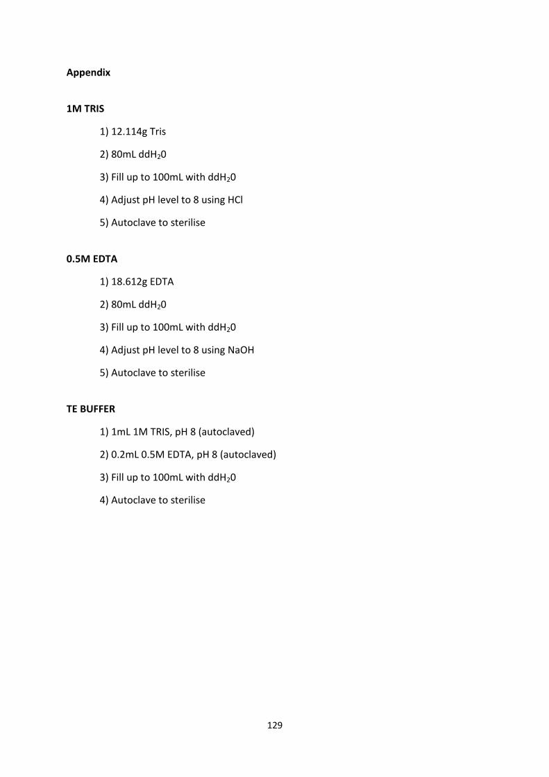
129

Appendix

1M TRIS

1) 12.114g Tris

2) 80mL ddH20

3) Fill up to 100mL with ddH20

4) Adjust pH level to 8 using HCl

5) Autoclave to sterilise

0.5M EDTA

1) 18.612g EDTA

2) 80mL ddH20


4) Adjust pH level to 8 using NaOH


TE BUFFER

1) 1mL 1M TRIS, pH 8 (autoclaved)

2) 0.2mL 0.5M EDTA, pH 8 (autoclaved)



Documents

The Role of Genomic Copy Number Variation (CNV) in ... · The Role of Genomic Copy Number Variation (CNV) in Osteoporosis Kate Connolly Bachelor of Forensics and Bachelor of Science