Embed Size (px)
Citation preview
CERDI, Etudes et Documents, E 2012.24
1
C E N T R E D ' E T U D E S
E T D E R E C H E R C H E S
S U R L E D E V E L O P P E M E N T
I N T E R N A T I O N A L
Document de travail de la série
Etudes et Documents
E 2012.24
The role of education and family background in marriage,
childbearing and labor market participation in Senegal
Francesca Marchetta
David E. Sahn
July 2012
CERDI
65 BD. F. MITTERRAND
63000 CLERMONT FERRAND - FRANCE
TEL. 04 73 17 74 00
FAX 04 73 17 74 28
www.cerdi.org

CERDI, Etudes et Documents, E 2012.24
2
Les auteurs
Francesca Marchetta, Clermont Université, Université d’Auvergne, CNRS, UMR 6587, Centre
d’Etudes et de Recherches sur le Développement International (CERDI), F-63009 Clermont-Ferrand,
France
Email : [email protected]
David E. Sahn
Cornell University, Ithaca, New York, and Clermont Université, Université d'Auvergne, CNRS,
UMR 6587, Centre d’Etudes et de Recherches sur le Développement International (CERDI), F-
63009 Clermont-Ferrand, France
tel. +33 (0) 473 17 74 07, fax. +33 (0) 473 17 74 28
Email: [email protected] (corresponding author)
La série des Etudes et Documents du CERDI est consultable sur le site :
http://www.cerdi.org/ed
Directeur de la publication : Patrick Plane
Directeur de la rédaction : Catherine Araujo Bonjean
Responsable d’édition : Annie Cohade
ISSN : 2114-7957
Avertissement :
Les commentaires et analyses développés n’engagent que leurs auteurs qui restent seuls
responsables des erreurs et insuffisances.

CERDI, Etudes et Documents, E 2012.24
3
Abstract
This paper examines the role of education and family background on age at marriage, age at
first birth, and age at labor market entry for young women in Senegal using a rich individual-
level survey conducted in 2003. We use a multiple-equation framework that allows us to
account for the endogeneity that arises from the simultaneity of the decisions that we
model. Differences in the characteristics of the dependent variable informed the choice of
the models that are used to estimate each equation: an ordered probit model is used to
analyze the number of completed years of schooling, and a generalized hazard model for the
other three decisions. Results show the importance of parental education, especially the
father, on years of schooling. We find that each additional year of schooling of a woman
with average characteristics delays marriage and the age at first birth by 0.5 and 0.4 years,
respectively. Parents’ education also reduces the hazard of marriage and age of first birth,
while the death of parents has just the opposite effect, with the magnitudes of effects being
larger for mothers. Delaying marriage also leads to an increase in the hazard of entering the
formal labor market, as does the education and death of the women’s parents.
Key Words: Multiple equations; duration models; unobserved heterogeneity; Senegal.
Acknowledgements
The authors are grateful to Simone Bertoli, Peter Glick, Chris Handy, Stan Panis, Paul Schultz
and Anne Viallefont for their comments and helpful suggestions on an earlier draft of this
paper. We also thank the participants at the Population Association of America (PAA) 2012
Annual Meeting and a seminar presentation at CERDI, Cornell University and the African
Development Bank. The usual disclaimers apply.

CERDI, Etudes et Documents, E 2012.24
4
1. Introduction
In a recent article, Ganguli, Haussmann, and Viarengo (2011) wonder whether the
narrowing of the gender gap in education in developing countries will contribute to closing
gaps in labor market participation, marriage and parenthood. These intertwined choices of
when to marry, begin a family, and enter the labor market are critical life-course decisions.
Understanding the relationships among them is complex, and the estimation of the effect that
each choice exerts on the others poses some key challenges because of the need to address the
issues of the endogeneity of decisions such as education and marriage. In addition, it is
necessary to deal with the related issue of unobserved heterogeneity, as different preferences
across women with respect to market work and children influence schooling and other
investments in human capital. Tackling these problems represents a formidable analytical
challenge. This paper analyzes the role of education and family background on age at
marriage, age at first birth, and age at labor market entry for young women in Senegal using a
rich individual-level survey conducted in 2003. We use a multiple-equation framework that
allows us to account for the endogeneity and the heterogeneity that arise from the simultaneity
of the decisions that we model, and we also introduce exclusion restrictions in order to
improve identification. Our results highlight the importance of own education in delaying
marriage, and that the impact of education on risk of childbearing and labor market entry is
mainly channeled through the age at marriage. We also show how the characteristics of the
parents differently shape women’s behavior: while mother’s education strongly influences
marriage and fertility choices, the education of the father is found to be more important in
affecting education and labor market choices.
This paper is related to a vast literature. There is considerable evidence of a robust
negative association between female education and fertility (Schultz, 1997), although it is
common to find such a result only for high levels of education for African countries

CERDI, Etudes et Documents, E 2012.24
5
(Younger, 2006; Appleton, 1996; Thomas and Maluccio, 1996). Several explanations can be
found for this negative relationship: woman’s higher education increases the opportunity cost
of childbearing (Becker, 1981), improves child health and reduces child mortality (Schultz,
1994), improves the knowledge of contraceptive methods (Rosenzweig and Schultz, 1985)
and increases the female bargaining power in fertility decisions (Mason, 1986). Even if the
correlation between education and fertility is robust, this needs not to reflect a causal
relationship: omitted variables, such as unobserved preferences or household or community
resources, can affect both schooling and fertility choices. Addressing this problem is a major
challenge, with a good example of doing so being the work of Osili and Long (2008) who use
the exposure to a program that involved investment in local schools in Nigeria as an
instrument that is not related to fertility outcome.
While education is often seen as crucial to success in the labor market, the challenge
that pervades the literature on the interrelation between work and schooling is that the level of
education is endogenous. This applies to various strands of the literature, including studies on
child labor where school and work are often seen as conflicting choices, and the literature that
analyzes the relationship between education level and labor market participation for young
women, who are assumed to make their participation decision after having acquired the
desired schooling level.1 There are a few studies that succeed in simultaneously modeling the
schooling and labor decisions using different estimation techniques: multiple stages models
(Ray, 2002), ordered probit models based on a ranking of schooling and employment
outcomes (Maitra and Ray, 2002; Kruger, Soares, and Berthelon, 2007), multinomial models
1 In the case of the child labor literature, Basu and Van (1998) argue that parents send children to school when
wages are high enough for them to earn a living without resorting to children’s labor to contribute to family
needs, Dessy (2000) shows that there is a critical level of adult wages under which child labor is supplied. In
contrast, however, Duryea and Arends-Kuenning (2003) find that the incidence of child labor is higher and
educational outcomes are lower in areas characterized by higher average wages; and Kruger (2007) reports that,
in coffee-producing regions, children are more likely to work (and less likely to go to school) during periods of
coffee booms.

CERDI, Etudes et Documents, E 2012.24
6
to simultaneously estimate the determinants of participation in school and work (Levison,
Moe, and Knaul 2001), and bivariate probit models (Wahba 2006) which take into account
that schooling and work choices are correlated.
In the strand of literature that shares our focus on labor market participation of young
women, the impact of education is often viewed as dependent on a constellation of factors that
go beyond schooling, and instead reflect the cultural context and social norms regarding
gender roles. There are two main pathways through which schooling positively affects
participation: through higher wage offers, and through the expectation that education
increases the bargaining power in the household (see, for example, Cameron, Dowling, and
Worwick, 2001). Still, as in the child labor literature, the empirical work on the impact of
education on young women’s entry into the labor market has failed to convincingly deal with
the joint nature of these decisions; and the same critique of the failure to address endogeneity
applies to most work that examines the links between marriage, fertility, and labor market
participation. Becker’s (1973, 1981) seminal contributions recognize that child rearing is
costly, especially for the mother; the increase in the value of mother’s time as a result of
investments in education and expanding career opportunities will affect the relative cost of the
children, thus reducing the demand. Many studies have empirically tested Becker’s theory
using education level as a proxy for the value of time and generally find that higher education
levels are associated with lower fertility rates (Schultz, 1997). Liefbroer and Corijn (1999)
discuss the empirical literature on the effects of education and woman labor participation on
marriage and childbearing in developed countries, showing that stronger effects are found for
parenthood rather than for marriage (see, for instance, Blossfeld and Huinink, 1991; De Jong
Gierveld and Liefbroer, 1995). The main problem is that education (and labor participation)
can be endogenous to the fertility choice: strong preferences for market work may induce
women to invest more in education and to have fewer children. Among the early work that

CERDI, Etudes et Documents, E 2012.24
7
attempts to explicitly address this problem is the study by Waite and Stolzenberg (1976), who
hypothesize the existence of a simultaneous reciprocal causation between fertility
expectations and labor force participation. Browning (1992) subsequently reviewed the papers
that try to tackle the issue of the possible endogeneity of fertility in the labor market supply
and affirms, “although we have a number of robust correlations, there are very few credible
inferences that can be drawn from them” (p. 1435). Another innovative approach to deal with
this endogeneity problem is that of Horz and Miller (1988) who hypothesize that, in each
period of time, parents choose a level of contraception and the amount of time a mother
allocates to the competing needs of child care, homemaking, and work in the labor market.
They use a four-equation system to model child care, labor participation, wages, and the use
of contraceptives, and find that there is a trade-off between the time spent for child care and
the time spent in the labor market.
Life-cycle models have also been extensively used to model the relationship between
fertility and female labor supply (Heckman and Willis, 1975; Moffit, 1984). Van der Klaauw
(1996) builds a dynamic utility maximization model using longitudinal data from a US panel
survey, where he predicts changes in the life-cycle pattern of employment, marriage, and
divorce due to differences in education, race, earnings, and husband’s earnings. In the model,
the sequential choices are interdependent, in the sense that all the previous choices have an
effect on current choices and preferences; for instance, wages depend on previous work
experiences. Similarly, Ma (2010) builds a structural dynamic model where, in each period
over her life cycle, a woman maximizes the expected discounted value of her utility by
simultaneously determining what category of occupation to enter into (professional, non-
professional, or housework), whether to be married, and whether to use contraception. There
are several papers which have tried to deal with the endogeneity of fertility in the participation
decision by adopting an instrumental variable approach. Rosenzweig and Wolpin (1980) rely

CERDI, Etudes et Documents, E 2012.24
8
on the use of sources of unplanned birth, like the presence of twins, while Rosenzweig and
Shultz (1985) use the availability and cost of contraceptive technology. Similarly, Bailey
(2006) uses the variation in the state-level legislation on access to the contraceptive pill, while
Angrist and Evans (1998) use parental preferences for a mixed sibling-sex composition. Less
effort has been made to tackle the endogeneity of marital status in the decision to enter the
labor market. Assaad and Zouari (2003), are an exception in this respect; they estimate a
structural model that takes into account the endogeneity of fertility and of the timing of
marriage in the participation decision.
The works by Angeles, Guilkey, and Mroz (2005), Brien and Lillard (1994),
Upchurch, Lillard, and Panis (2002), and Glick, Handy, and Sahn (2011) provide the most
direct guidance for the approach we adopt in this paper. Angeles, Guilkey, and Mroz (2005)
study the effect of education and family planning on fertility in Indonesia. They jointly
estimate education level, age at marriage, and fertility, using maximum likelihood procedures
that assume that the heterogeneity terms of the three equations are correlated. The joint
distribution of the unobservables is incorporated using a semi-parametric discrete factor
method, as suggested by Heckman and Singer (1984) and extended by Mroz and Guilkey
(1995) and by Mroz (1999). They report that, controlling for the endogeneity of education and
marriage, the impact of the increase of education in reducing fertility is quite low. Conversely,
they find that family planning services are very effective in reducing fertility in Indonesia.
Brien and Lillard (1994) study the interrelations between education, timing of
marriage, and timing of first conception in Malaysia. They build a sequential probit model to
estimate the schooling decision and model the timing of marriage and first conception through
hazard models, allowing for correlation among the heterogeneity components of the three
CERDI, Etudes et Documents, E 2012.24
9
equations.2 Identification is possible thanks to the hypothesis that, for each equation, there is a
common heterogeneity component for sisters and that, conditional on this component, sisters’
behaviors are otherwise independent. They find that education significantly delays the age at
marriage, and that the increase in the age at first conception is due to the delayed marriage.
Brien, Lillard, and Waite (1999) estimate entry into marriage, cohabitation, and non-
marital conception using a similar framework. They model each outcome with a continuous
hazard model, and they account for the simultaneity of the three related processes. In this
case, they are able to observe multiple episodes of each outcome for a subsample of women,
and this allows for the identification of the degree of variation in individual specific
components for each outcome and the correlation among those components. The same
framework is used by Upchurch, Lillard, and Panis (2002), who estimate a model where
education, marriage, and fertility decisions influence one another and where each outcome is
affected by a woman’s characteristics. They find that the risk of conceiving depends on
education for white and Hispanic women, but not for black women, while all women make
simultaneous choices regarding childbearing and marriage.
More recently, Glick, Handy, and Sahn (2011) have examined the relationships among
education, age at marriage, and age at first birth in Madagascar, with a multiple equation
model, showing that schooling is very effective in delaying marriage and childbearing. Our
paper extends their approach, as we not only jointly estimate the determinants of education,
age at marriage, and age at first birth, but also age at entry in the labor market for young
women in Senegal. We assume that there are common factors that influence the four
behaviors we are analyzing. Some of these factors are observable, like parents’ education,
2This model is a combination of the simultaneous equations for hazard models by Lillard (1993) and the
sequential choice model of education by Lillard and Willis (1994).

CERDI, Etudes et Documents, E 2012.24
10
household wealth, characteristics of the place of residence, and so on. Some other factors are
unobserved, like, for example, women’s preferences.
Moreover, our main interest is in understanding the role of education and family
background on labor supply, and identifying both the direct impact, as well as indirect impact
mediated through marriage and fertility. For example, a women’s education will presumably
facilitate entry into the labor market. But there is also an indirect effect of education on labor
market choices, to the extent, for example, that more education contributes to postponing
marriage and childbearing, the timing of which also affects labor market choices.
In order to take into account for all these interrelations, we use a multiple equation
framework. Differences in the characteristics of the dependent variable informed the choice of
the models that are used to estimate each equation: an ordered probit model is used to analyze
the number of completed years of schooling; hazard models are used to analyze age at
marriage, age at first childbearing, and age at entry in the labor market. Our estimation
approach is fully consistent with the theoretical description of the determinants of these key
decisions, and it extends those adopted in Brien and Lillard (1994), Upchurch, Lillard, and
Panis (2002), Angeles, Guilkey, and Mroz (2005), and Glick, Handy, and Sahn (2011).
As in Brien and Lillard (1994), we identify the covariance matrix of unobserved
heterogeneity components, assuming that sisters share identical heterogeneity components for
each equation. Moreover, we rely on exclusion restrictions: we identify the completed years
of education using detailed retrospective information on local schools and the age at marriage
through the use of information on the marriage market. We use the information on the timing
of the introduction of family planning programs at the community level in order to identify
the age at first childbearing. Finally, we use the information on labor market shocks to
identify the decision to enter the labor market. In all these cases, we rely on retrospectively
collected data. While we are comfortable with these exclusion restrictions, even in the

CERDI, Etudes et Documents, E 2012.24
11
absence of instruments we are able to deal with the unobserved heterogeneity through our
estimation technique; our exclusion restrictions can thus be considered largely a bonus, as
emphasized by Lillard (1993) and Brien, Lillard, and Waite (1999) and discussed further
below.
In the remainder of this paper, we begin with a discussion of the empirical strategy in
Section 2, followed by a presentation of the data we use in Section 3. Section 4 presents the
main results, and Section 5 concludes.
2. Empirical Strategy
We simultaneously model four key decisions in a woman’s life course: (i) the level of
education, (ii) the age at marriage, (iii) the age at first birth, and (iv) the age of the initial entry
in the formal labor market3.
We model the number of grades completed for woman � living in community �, with
an ordered probit model. An individual will have � grade of schooling, ��� � �, if � ���∗ �� , where ���∗ is the latent continuous variable that generates the observed ���, and � and
�� are the cut-off points to be estimated. Equation (1) describes the determinants of the
latent variable ���∗
���∗ � ��� � � �′��� � ���′�� � ���′���� � ���� (1)
��� is a vector of individual and household characteristics, including age, information on the
father’s and mother’s education, ethnicity, religion, region of birth, whether resident is in a
rural or urban area, and whether the mother and father are dead. To avoid reverse causality,
we also include information on the housing assets of a woman when she was 10 years old and
information on the availability of health infrastructures, also measured when the woman was
3 We define the formal labor market as comprising entrepreneurs and waged work, both in the private and in the
public sectors. The private sector includes household enterprises.

CERDI, Etudes et Documents, E 2012.24
12
10 years old. �� is a vector of community-level factors, including the widespread access to
electricity, the availability of piped water, and presence of three types of credit institutions ─
micro-credit institutions, insurance institutions that offer credit, and small individual lenders.
���� is a vector of school characteristics, including the share of local teachers in the closest
primary school with at least five years of experience and the number of years of education of
the school director. It also includes information on access to primary and secondary schools
when the woman was 10 years old, again since the choices about schooling investments were
likely made on the basis of information on school access when children were young, not as
adults when schooling is complete. We use the notation���� to indicate a vector of variables
that are included in the schooling model but excluded from the other equations. ���� � ���� �
���� , where ���� represents unobserved characteristics which influence the grades completed by
a woman � living in community �, and ���� follows an identically and independently distributed
normal distribution, i.e., ���� �~��� 0, #��$.
We model the age at marriage with a proportional hazard model, as it is represented in
Equation (2):
ln'��( )$ � ��( � � (*+,�� )$ � ��(′��� � ��(′�� � �-(��� � �.(/��(����( (2)
where '��( )$ represents the ratio between the probability of getting married at time t over the
cumulative probability of not having married up to time t. The baseline hazard is represented
by a generalized Gompertz model, which allows the baseline hazard rate to be a non-
monotonic function of time; *+,�� )$ is the piecewise linear duration dependency spline. The
risk of marriage begins at age 11. Thus:
� ( )$ � 0 � ( ) �1) 2 ) � ( ) � � �( ) 3 ) $ �1) 4 )
CERDI, Etudes et Documents, E 2012.24
13
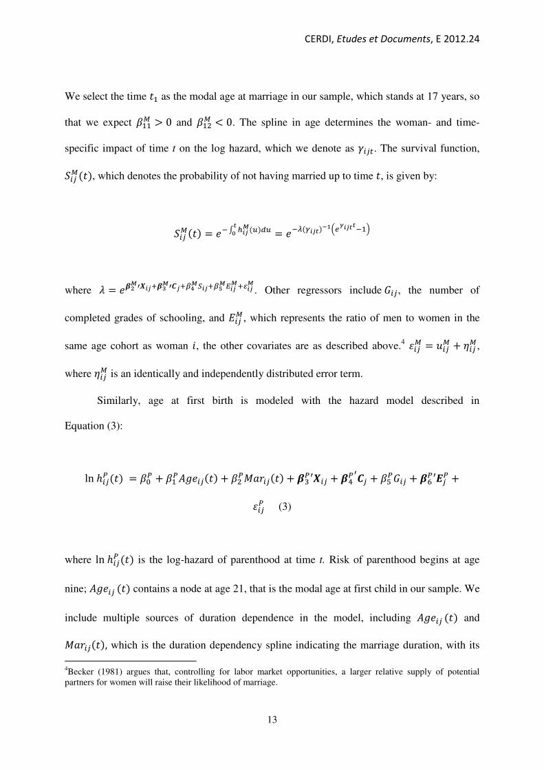
We select the time ) as the modal age at marriage in our sample, which stands at 17 years, so
that we expect � ( 4 0 and � �( 0. The spline in age determines the woman- and time-
specific impact of time t on the log hazard, which we denote as 5��6. The survival function,
7��( )$, which denotes the probability of not having married up to time ), is given by:
7��( )$ � ,89 :;<= >$�>?@ � ,8A B;<?$CDEFG;<??8 H
where I � ,�J=K�;<��L=K�<�MN=O;<�MP=Q;<=�R;<=. Other regressors include���, the number of
completed grades of schooling, and /��(, which represents the ratio of men to women in the
same age cohort as woman �, the other covariates are as described above.4 ���( � ���( � ���(,
where ���( is an identically and independently distributed error term.
Similarly, age at first birth is modeled with the hazard model described in
Equation (3):
ln'��S )$ � ��S � � S*+,�� )$ � ��STUV�� )$ � ��S′��� � �-SK�� � �.S��� � �WS′��S �
���S (3)
where ln'��S )$ is the log-hazard of parenthood at time t. Risk of parenthood begins at age
nine; *+,�� )$ contains a node at age 21, that is the modal age at first child in our sample. We
include multiple sources of duration dependence in the model, including *+,�� )$ and
TUV�� )$, which is the duration dependency spline indicating the marriage duration, with its
4Becker (1981) argues that, controlling for labor market opportunities, a larger relative supply of potential
partners for women will raise their likelihood of marriage.
CERDI, Etudes et Documents, E 2012.24
14
coefficient allowed to change after three years since marriage.5 ��S is a vector of exclusion
restrictions (including the availability of condoms in the community and the year when they
were first available). ���S � ���S � ���S , where ���S is an independently and identically distributed
error term.
Finally, Equation (4) presents the hazard model for age at entry in the formal labor
market:
ln'��X )$ � ��X � � X*+, )$ � ��XTUV�� )$ � ��XYUV�� )$ � �-X��� � �.X�� � �WX��� �
�ZX���X � ���X (4)
where ln'��X )$ is the log-hazard of entry in the labor market at time t. Risk of labor starts at
age five, and *+,�� )$ contains a node at the modal age at entry in the formal labor market,
that is 15 years. ���X is a vector of dummies, indicating if a positive or a negative shock in the
labor market occurred after leaving school6; YUV�� )$ is the duration dependency spline
indicating time since first child, and its coefficient is allowed to change after two years since
the birth of the first child. ���X � ���X � ���X , where ���X is an independently and identically
distributed error term.
Individual unobserved heterogeneity poses two main challenges to our efforts to
estimate these four interrelated outcomes. Observations with the same values for all covariates
are not identical in terms of their hazards: some are more likely to experience failures than
5 We have also tried including in the model a duration dependency spline indicating the time elapsed since labor
market entry, but it turned out not to be significant. 6 The positive economic shocks that may have occurred in the community are the establishment of a new
enterprise, the building of a new road, the establishment of an electric plant, of an irrigation system, of a piped
water system, or of another development project, and a period of good pluviometry. The negative economic
shocks that may have occurred are a fire, a flood, a period of drought, a massive damage to the harvest or to the
livestock, or the closure of an enterprise.

CERDI, Etudes et Documents, E 2012.24
15
others because there are unobservables in the error term, ���, that influence the decision
processes that we are going to analyze. Ideally, we would identify the two different terms
contained in ���: the random error term (���) and the unobserved heterogeneity component
term ���).
The second main challenge is represented by the fact that the unobserved factors that
appear in Equations (1)–(4) are likely to be correlated, i.e., the same unobserved individual-
specific characteristics simultaneously influence the four decisions we want to model. If this
is the case, these influences give rise to an endogeneity problem. Consider, for instance, the
completed grades of schooling ��� which appear on the right side of Equations (2)–(4): ��� is
determined by ���� , thus whenever [\VV]���� , ��� ^ _ 0, with � � T, Y, `, then ��� will be
correlated with the unobserved component of the error terms in Equations (2)–(4), and ���
will thus be an endogenous regressor.
In order to deal with these challenges, we opt for an estimation strategy that is
consistent with the fact that the decisions about schooling, marriage, childbearing, and labor
market participation are interrelated, and we jointly estimate the four models. We consider
these decisions as interrelated in the sense that they are all influenced by individual
characteristics, and that some of the endogenous outcomes of interest have a direct impact on
other outcomes. Some of these characteristics are observed, while others are unobserved. We
assume that, after conditioning on all observed variables, the heterogeneity term captures all
sources of correlations among the four decision processes. The likelihood functions of each of
the four models are independent if we are able to condition for the relevant observed and
unobservable characteristics. If this is the case, the joint conditional likelihood of the set of
observed outcomes for the four decision processes is the product of the conditional
probabilities of the four models.

CERDI, Etudes et Documents, E 2012.24
16
Identification of our four-equation system requires adding some structure on
unobservable factors. Ideally, if we were able to repeatedly observe the choices made by a
single woman under different observable conditions, we could control for the invariant
unobserved component of the error term. The multiple outcomes per woman would allow
separating the observation’s specific heterogeneity component, (���), from the random error
term, (���). Our data do not allow for such an ideal setting, so we need to introduce
assumptions which allow us to identify the covariance matrix of unobserved heterogeneity
components. Since we do not have repeated outcomes for the same individual, we assume that
all the sisters living in the same household share identical heterogeneity components for each
equation, as in Brien and Lillard (1994). This is a reasonable hypothesis since sisters are
exposed to the same family circumstances and come from the same background, i.e., the same
social context and the same value system. This assumption allows for the estimation of the
degree of variation in the sisters-specific component for each process and the correlation
among these components.
As described above, each equation contains exclusion restrictions, i.e., covariates that
are included only in one equation and are excluded from the others. However, these are not
essential in order to identify the model (Lillard, 1993; Brien, Lillard, and Waite, 1999) 7
. The
software we use for this analysis is aML (Lillard and Panis 2000).
2.1. Marginal effects
The computation of the marginal effects of any regressor needs to account for both the
direct effect on each of the four models, as well as for the indirect effects that go through the
outcomes of earlier models, as our four-equation system is recursive.
7 We have also run the model without the exclusion restrictions. The estimated coefficients are not statistically
different across the two models (with the exception of the intercept of the fertility model). We computed the
likelihood ratio test (LRT) to compare the two models: the test follows a χ²(13) distribution under the null; the
test statistic is 261.63 and it strongly rejects the null, suggesting that the less restrictive model (the one with the
exclusion restrictions) fits the data better.

CERDI, Etudes et Documents, E 2012.24
17
Let a�� denote all the possibly regressors which are included in at least one of the four
models; without loss of generality, assume that the first element in a�6 is a continuous
variable.8 The partial derivative of the predicted number of completed grades/]�ba��^, with
respect to c ��, is given by:
d/]�ba��^de ��
� fdYV\g]� � �ba��^de ��
�h
i� � f� �ϕ]� 3 kZmno^
h
i�
Then, we compute the impact of the marginal variation in a��6 upon the median age at
marriage9 as predicted by the duration model in Equation (2). This, in turn, depends on (i) the
direct impact captured by the estimated coefficient in Equation (2); and (ii) the impact which
goes through the influence of the variation in /]�ba��^.
Similarly, the influence of a marginal variation in a�� upon the parenthood model in
Equation (3) has to account for its influence upon the timing of the marriage. To give an idea
of the richness of these indirect effects, we can observe that the influence of, say, the death of
the father upon the age of entry in the labor market of a woman in the sample depends on 17
coefficients estimated in the four models.
3. Data Sources and Descriptive Statistics
The data we use in this paper is the 2003 Household Survey on Education and Welfare in
Senegal (EMBS), conducted in 33 rural and 30 urban communities.10
Although, as discussed
by Glick and Sahn (2009, 2010), the EMBS sample is not truly nationally representative, it is
part of a cohort study of young children, and efforts were made to randomly select into the
8If one element of this vector is excluded from model ' with ' � �,T, Y, `, then its coefficient is constrained to
zero. 9This is defined as the predicted age at marriage at which 7��( )$ is equal to 0.5; no closed form expression exists
for the mean time to failure predicted by a Gompertz model. 10
See Glick and Sahn (2009, 2010) for details about the survey design.

CERDI, Etudes et Documents, E 2012.24
18
sample new households to ensure that it is as close as possible to a random sample.
Indications from comparison with other national surveys indicate that this effort was quite
successful, and that the sample of 1,820 households is representative of the population in
terms of religion, ethnic groups, and demographic characteristics, as well as other
characteristics such as education.11
Our sub-sample consists of 2,668 females between the ages of 15 and 30 years of age. The
number of sisters in the sample varies from zero to seven, and 1,212 women have at least one
sister which is sufficient to estimate the sibling specific heterogeneity component.
In our analysis, we rely extensively on the education, labor market, and demographic
modules of the EMBS, as well as the module which contains information on the current
residence, and on retrospective questions for adults above age 21 about where they lived, as
well as the household and community characteristics, when they were 10 years old. These
data are a key component of our methodology, as they allow us to observe the childhood
characteristics that we use to explain the marriage, fertility, and labor market decisions. We
also use the community and school modules that collect detailed information on the local
infrastructure in general, as well as the characteristics of schools in the community. This
includes the experience and credentials of the principal and management of the school, as well
as the number of teachers, their qualifications and pedagogical practices. These are used as
control variables in the analysis that follows. In addition, we have information about the
availability of family planning services and the availability of contraceptive devices, all of
which were collected as part of the community survey. In each community, it was determined
whether each service type was available and, if so, when it first became available.
11
For example, net primary enrollment in our sample (primary enrollments of children 7–12) is 66 percent
compared with 63 percent for the country as whole in 2000 (World Bank, 2006).

CERDI, Etudes et Documents, E 2012.24
19
Thirty two percent of the women in the sample are married, 24 percent are parents and
21 percent are married with a child. Birth before marriage occurs for 10 per cent of the
women who have a child12
. Just half of them got married within two years after childbearing,
so that we can assume that childbearing has a direct effect on marriage decision only for about
1.3 percent of the sample. This is why we decided not to consider this effect in our model.
Childbearing before schooling dropout is not common: four women had a child before
leaving school, six in the same year and seven one year after. This implies that the direct
effect of childbearing on schooling is negligible in our sample, and it can be ignored when
modeling women’s choices.
Around 18 percent of our sample report working in the formal sector labor market, and
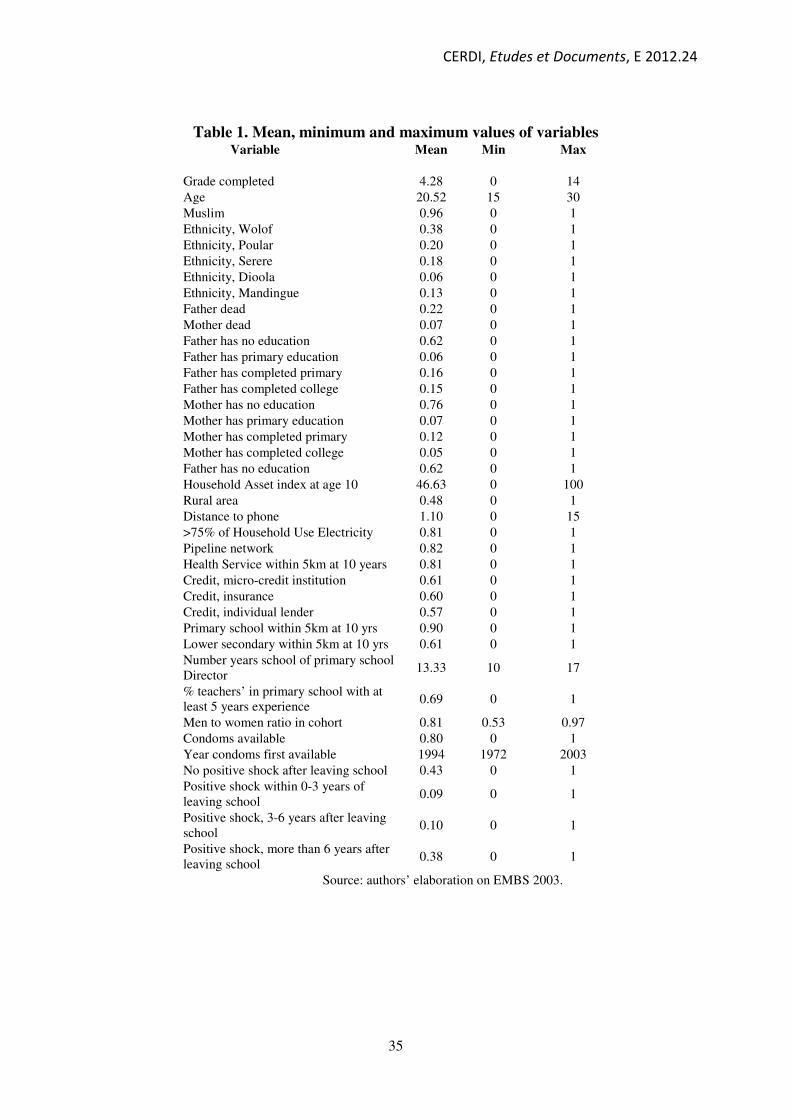
the average age of entry is 17. Descriptive statistics for variables used in this paper are
reported in Table 1 and indicate that the average age of women in our sample is 20.52, that
they have an average of 4.28 years of schooling, although 25 percent of the women are still in
school. Thus, mean completed school among this cohort will be higher. Only 36 percent of
their fathers and 23 percent of their mothers attended some school.
About half of our sample is rural, and it is 96 percent Muslim. The largest ethnic group
is Wolof, comprising 38 percent of the sample, followed by the Poular and Serere, each
representing approximately one-fifth of the sample. Ninety-percent of women lived in a
community with a primary school within 5 km at age 10, while only 61 percent lived in a
community with a lower secondary school within the same distance. Among other community
infrastructure, around four out of five communities have piped water, electricity, and readily
available condoms, with the average year that condoms became available being 1994.
Approximately 60 percent of the communities report having access to each of the following
types of credit sources: micro-credit, insurance, and individual lenders. However, among our
12
Three per cent of sample women have a child but are not married.

CERDI, Etudes et Documents, E 2012.24
20
communities, 25 percent have none of these sources, 24 percent have only one of these
sources, and 51 percent have all three of these sources of credit.
4. Results
We present the results of the 4-equations model in Table 2 and 3, where we report the
coefficients and the t-statistics of the joint estimation. We provide the marginal effects of the
key variables of the models in Tables 4 and 5.
4.1 Education
We find that the education of the mother and of the father have a powerful impact on
schooling attainment of their daughter. Interestingly, the magnitude of the coefficients of
father’s education is substantially higher than that of the mother. When we compute the
marginal effects, we find that if the mother has some primary schooling, the impact on her
daughter’s education is modest, just 0.03 years. However, if the mother has completed
primary school, the daughter is estimated to have completed 0.67 additional years of school. If
the mother has at least completed lower secondary school, the predicted effect on schooling of
the daughter just about doubles to 1.4 years of schooling. The impact of a father’s education is
much greater; a daughter of a father who has completed primary school will have 1.2
additional years of schooling, with the comparable number of lower secondary schooling
being 1.9 more years for his daughter, as compared to a father with no schooling. The death
of a father reduces the expected years of schooling by around 0.45 years; no such effect is
observed for the death of a mother, as indicated by the insignificant parameter estimate. One
plausible explanation for this is that the father’s death has a greater impact on household
resources and thus contributes to an earlier school dropout. However, we would have
expected that girls substitute in terms of home production when their mother dies even though
work at home and schooling are not mutually exclusive activities.

CERDI, Etudes et Documents, E 2012.24
21
The household asset index when the girl was 10 years of age also has the expected
positive impact on schooling outcomes. As mentioned above, relying on this lagged asset
variable avoids the possibility of any reverse causality and more accurately reflects how
wealth at or around the time that a child is just enrolling in school affects long-term schooling
outcomes. In terms of magnitudes, we find that an increase in the asset index of one standard
deviation contributes to 0.45 year increase in the number of years of schooling.
A child living in a community with a primary school within 5 km when she was 10
years old is expected to have completed 2.8 more years of school than a child living in a
community without such a school. The presence of a lower secondary school within 5 km, at
10 years of age, has about one-third the impact on schooling than the presence of a primary
school.
Among schooling characteristics, our results indicate that each year of additional
education of the director increases the expected level of education by 0.04 years. Similarly, a
10-percentage point increase in teachers with at least five years of experience raises the
expected years of schooling by 0.07 years. Some caution is warranted in interpreting these
school characteristics variables since it is possible that community heterogeneity is driving the
results. While we cannot rule this out, we include a range of other community covariates to
deal with this problem. Included are indicator variables that capture whether most of the
households have access to electricity, whether there is piped water available, the distance to
land-line telephones, and the presence of various credit institutions, as well as access to health
facilities when the women were 10 years old. These are largely intended as controls, and thus
caution is necessary in interpreting the individual parameters in a causal fashion13
.
13
Among other marginal effects of note is that Muslim girls are expected to complete 0.9 less years of schooling
that other religious groups, and among the Diola ethnic group, 0.7 years more than the predominant Wolof ethnic
group. Being born in certain regions also results in far lower schooling achievement. For example, those from
Diourbel complete 0.68 fewer years of schooling, and conversely, those born in Louga complete more schooling
than the region of Dakar (results not shown).

CERDI, Etudes et Documents, E 2012.24
22
4.2 Marriage
In considering the determinants of marriage, we concentrate our discussion on the
presentation of the total marginal effect, which includes both the direct effect as well as the
indirect effect of the parameters, operating through the grade attained as well as the normal
aging process that is captured separately by the age splines that affect the timing of marriage.
One of the most notable results is that each additional year of schooling delays the median age
at marriage by approximately half a year (and a one standard deviation increase in the number
of completed grades delays marriage by 2.22 years)14
. In examining the impact of the
characteristics of the household in which the woman lived when she was a child, we find that
the women’s mother and father having some education increases the survival probabilities in
the non-marital state, and the deaths of a mother and father have the opposite effect, raising
the hazard of entering into marriage. More specifically, the time to marriage among women in
our sample is increased by 4.01 years when their mothers have primary education, nearly four
times the magnitude of the effect of their fathers having primary education. The effect of the
death of a mother reduces the survival function by nearly two years. Interestingly, we find
little effect of a father’s death on hazard of marriage. We also find that the higher the ratio of
men to women, the higher the hazard of getting married. This is consistent with our
expectations insofar as the more men relative to women in the local marriage market, the
shorter the survival time to marriage15
.
14
Other individual characteristics that seem to be important in terms of affecting the marriage hazard include
that of being a Muslim, which decreases the survival time to marriage by a great deal, 3.76 years; being a
member of the Pular ethnic group increases the hazard of marriage by 2.35 years (results not shown). 15
The economic literature evidences the possible impact of sex ratio on labor market participation of women.
Angrist (2002) shows that a high sex ratio has a negative effect on female labor market participation. The idea is
that women who expect to get married have less incentives to be engaged in the labor market. We have tested for
the existence of an effect of sex ratio on age at entry in the formal labor market and we did not find such a
relationship in our sample. This allows us to use the sex ratio as an exclusion restriction in the marriage model.
CERDI, Etudes et Documents, E 2012.24
23
4.3 First birth
Figure 1 presents the survival functions for marriage and age at first birth for a representative
woman16
. The survival probability function for marriage crosses the 50 per cent probability
line around 23 years of age, and by her late twenties, this woman is expected to have married.
The risk of childbearing increases rapidly after marriage – represented by the first vertical line
in Figure 1 - and especially during the first three years of marriage17
Like with marriage, the women’s own education and that of her parents are of critical
importance in terms of the timing of first births. An additional grade of education increases
time to first birth by 0.41 years (and a one standard deviation increase in the number of
completed grades delays first birth by 1.28 years). The mother having some primary education
delays the age of first birth by 1.8 years, which is over two times the magnitude of the effect
of the father having some education.
In modeling the hazard of first birth, we find that the coefficients on the time since
marriage, as entered as a spline for the first three years, and more than three years of
marriage, have the expected positive sign and are statistically significant at standard levels.
This can be interpreted as suggesting that the hazard of having a first birth increases with time
during the first three years of marriage, and thereafter, it remains stable. In terms of the
magnitude of the impact, delaying marriage by one year (i.e., decreasing marriage duration by
one year) increases the median parenthood age by 0.61 years. This is portrayed in the survival
function shown in Figure 2.
The death of the women’s mother also has a large impact on the hazard of first birth,
the magnitude being nearly as great as impact on marriage. The death of a father has a smaller
16
This woman takes the average characteristics of married parent women (mean value for continuous variables
and modal value for dummies and discrete variables). 17
There are 73 women in a polygamous marriage. We ran the model with a dummy variable for women living
with polygamous husbands in the fertility and labor market models, and both were insignificant.

CERDI, Etudes et Documents, E 2012.24
24
impact than the death of a mother, although, the impact on first birth is still quite high,
reducing the survival time by 0.66 years. 18
We also find that the availability of condoms and related family planning facilities in
the community reduces the hazard of first birth.19
The marginal effect implies that first birth is
delayed by 0.81 years when condoms and family planning services are available. However, in
those communities where condoms have been available for longer periods, condom
availability has a smaller impact on the hazard of motherhood. This might be explained by the
fact that there is a greater influence in the period which shortly follows the introduction of
condoms, both because of their novelty, as well as the possibility that more recent efforts at
condom diffusion are more effective in terms of broad-based behavioral change. Nonetheless,
we caution against a strict causal interpretation of the condom availability parameter for
reasons related to issues of program placement, as discussed elsewhere.
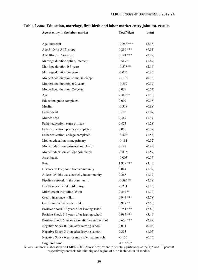
4.4 Labor market entry
The magnitude of the marginal effect of own education is relatively small, with each
additional grade of schooling reducing the survival function for not being engaged in paid
18
Table 2 shows that most of the other covariates that we include in the parenthood model are not significant.
This is not an unexpected result, given the high explanatory power of the marriage duration spline. The
correlation between age at marriage and age at first child is 0.63 and the difference between the two ranges
between zero and three years for seventy percent of the married women who had a child. If we run our 4-
equation model omitting the marriage duration spline, several covariates in the fertility model turn out to be
significant. This is the case, for instance, for the number of completed grades and the mother’s education. These
results, which are available from the authors upon request, are in line with Brien and Lillard (1994). 19
Condom availability might be endogenous with respect to childbearing, if familly planning services are placed
in the communities where higher levels of fertility prevail (Angeles, Guilkey, and Mroz, 1998). We follow
Portner et al. (2007) and instrument the availability of condoms using as explanatory variables the ranking of the
Senegalese departments on some key determinants of fertility rate, specifically population size, the rate of
urbanization, education, and the immigration rate. We built these ranking using the data from the 2002
population census. The underlying hypothesis is that, while the average characteristics of the department have an
impact on the individual fertility decision, the relative position of a department does not affect individual fertility
choices, and it can thus represent a valid instrument for the placement decision. We then compute the
generalized residuals (Gourieroux et al., 1987) from the first stage, including them as auxiliary regressors in the
non-linear fertility model together with the endogenous variables (Terza et al., 2008). Results show that the
generalized residuals are positive –suggesting that fertility planning services are placed in areas where the age at
first child is lower – but they are not significant at conventional confidence level – thus reducing our concerns
about the endogeneity of condoms availability.
CERDI, Etudes et Documents, E 2012.24
25
work out the household by 0.18 years (and 1 standard deviation increase in the number of
completed grades anticipates entry in the labor market by 0.42 years).20
In Figure 3 we draw
the survival function for entry into the labor market for a representative woman. By age 25,
she has an 8 percent expected probability of having begun paid work outside the home.
Having 3.5 additional years of schooling (corresponding to one standard deviation), this
figure would be closer to 11 percent. Most of the impact of grade attainment on the risk of
labor market entry passes through the influence of schooling on the timing of marriage and
parenthood. This explains why the two survival functions nearly coincide up until the age
when a woman is making decisions regarding marriage and fertility.
The hazard of entering the labor market increases as a result of a positive economic
shock having occurred in the previous six years, conditional upon having completed
schooling. Presumably, this reflects the greater opportunities for paid employment that are
associated with positive economic events that occur when a woman has exited school.
Conversely, any change in the hazard of entering the labor market is not affected by negative
shocks that occur after leaving school. This result seems plausible since a negative shock
would be expected to increase the impetus for a woman to find a job to cope with the stress of
the shock, but at the same time, a negative covariate shock may reduce the possibilities of
finding such a job.
The women whose father or mother has some primary schooling experience an
increased hazard of entering the formal sector. The marginal effects of a father having some
primary education are particularly high: the duration to entry into the formal labor market is
3.33 years shorter if the father has some education, more than twice the magnitude of the
20
The effect of education likely has two opposing influences on labor market entry, delaying entry of the women
who might queue longer in anticipation of a better wage offer, while at the same time enabling earlier entry due
to employers being more willing to hire women with better credentials.
CERDI, Etudes et Documents, E 2012.24
26
effect of the mother’s education. The death of a mother and a father also contributes to earlier
entry into the formal labor market, just like it does for marriage and age of first child.
We also consider how the time since marriage affects the entry into the labor market.
The negative and significant effect of being married for 0–3 years indicates that the hazard of
entering the labor market (the change in the instantaneous probability) decreases with time to
labor market entry during the first three years of marriage; thereafter, marriage duration has
no impact on the hazard of working outside the home. In terms of magnitude, delaying
marriage by one year reduces the expected time before entering the formal labor market by
0.31 years. The negative coefficients on the motherhood duration splines also suggest that the
hazard of entering the labor market decreases as a consequence of motherhood, although, the
effect is not statistically significant21
.
4.5 Heterogeneity correlations
Finally, in Table 3, we present the standard deviations and correlations of the
heterogeneity components. All of the standard deviations are significant, meaning that the
sisters-specific heterogeneity component is significant across the four processes. The
correlation between marriage and parenthood is positive and highly significant. This indicates
that women with a propensity to putting off marriage, share this with the decision to have a
first birth, and this correlation persists once we control for the direct effect of the marriage
duration on the age at first birth, and for all the other covariates.
The correlations between the other heterogeneity components are not statistically
significant. This suggests that the richness of our dataset allows us to control for covariates
21
Among the other covariates, Muslim women have the expected lower risk of entering the labor market. In fact,
the duration until formal labor market entry is expected to be 3.46 years longer for Muslim than non-Muslim
women. As with the other models, we include a range of community covariates, largely as control variables. We
do take particular note of the impact of accessibility of credit institutions in terms of increasing the hazard of job
entry.

CERDI, Etudes et Documents, E 2012.24
27
that are able to simultaneously determine the outcomes of interest. In light of this result, we
also run the model ignoring the correlations between the heterogeneity components to see if
the results are different once we treat schooling, marriage and childbearing as exogenous
variables in the other models. Table 6 presents the coefficients of the key variables for the
model without heterogeneity. When we restrict the correlation across equations to zero, the
results are not substantially different. But the magnitude and the significance of some key
coefficients vary, and the standard errors are generally lower. In particular, the magnitude of
the coefficients of the marriage duration spline in the parenthood model is larger and the
completed grade of education is significant in the parenthood model. We computed the
likelihood ratio test to compare the two models: the test follows a χ²(6) distribution under the
null. The test statistic is 24.62, meaning that our approach to allowing for the correlations
across equations to differ from zero fits the data better. We can conclude, as in Brien and
Lillard (1994), that, even if the model that controls for correlation in heterogeneity across
equations does not produce dramatically different results from the model that does not control
for this correlation, it is still preferred because it both produces consistent estimated
parameters and standard errors, and also provides a better overall fit of the data.
5. Conclusions
We have simultaneously estimated four key decisions in a woman’s life course, (i) the
level of education, (ii) the age at marriage, (iii) the age at first birth, and (iv) the age at entry
in the formal labor market, through a recursive model which allows for common unobserved
factors, and controls for the endogeneities that result from the joint determination of these
outcomes. We identified the covariance matrix of unobserved heterogeneity components,
under the assumption, which was first suggested by Brien and Lillard (1994), that sisters share
identical heterogeneity components for each equation. Exclusion restrictions, which are not

CERDI, Etudes et Documents, E 2012.24
28
necessary to identify each equation (Lillard, 1993; Brien, Lillard and Waite, 1999) have also
been added.
Our main goal was to gain some insight into the links between these simultaneously
determined choices in order to better understand the importance of individual attributes and
family background. We highlight the importance of factors when the woman was 10 years old
in determining her schooling attainment. These include parents’ education, the death of the
father and the wealth of the parents’ household. Our paper’s main focus, however, is on the
effect of schooling and family on the other outcomes that we model. We find that the number
of completed grades is important in delaying marriage and the age at first birth. This effect of
education on fertility operates mainly through delayed marriage, consistent with the findings
of Brien and Lillard (1994). We also observe that marriage and childbearing decisions are
simultaneously determined by unobserved factors, as in Brien, Lillard and Waite (1999).
Education also eases entry into the labor market, again with the effect operating mostly
indirectly through a delay in marriage. Among the variables capturing the family background,
parents’ education strongly influences women’s behavior: mother education has a greater
influence on marriage and fertility choices, while education of the father is found to be more
important in affecting education and labor market choices. The death of the parents are also
important in affecting all the outcomes of interest, and the impact of the death of a mother is
far larger than the father, except for completed grades.
CERDI, Etudes et Documents, E 2012.24
29
References
Angeles, G., Guilkey, D. K., and Mroz, T. A. (2005) The effects of education and family
planning programs on fertility in Indonesia. Economic Development and Cultural Change
54(1): 165–201.
Angeles, G., Guilkey, D. K., and Mroz, T. A. (1998) Purposive Program Placement and the
Estimation of Family Planning Program Effects in Tanzania. Journal of the American
Statistical Association, 93(443): 884-899.
Angrist, J. (2002) How Do Sex Ratios Affect Marriage And Labor Markets? Evidence from
America's Second Generation. The Quarterly Journal of Economics 117(3): 997-1038.
Angrist, J., and Evans, W. (1998) Children and their parents’ labor supply: Evidence from
exogenous variation in family size. American Economic Review 88(3): 450–477.
Appleton, S. (1996) How does female education affect fertility? A structural model for the
Côte d’Ivoire. Oxford Bulletin of Economics and Statistics 58(1): 139–166.
Assaad, R., and Zouari, S. (2003). Estimating the impact of marriage and fertility on the
female labor force participation when decisions are interrelated: Evidence from urban
Morocco.” In Cinar, E. M., (ed.), Topics in Middle Eastern and North African Economies
(electronic journal), Vol. 5. Chicago: Middle East Economic Association and Loyola
University Chicago.
Bailey, M. J. (2006) More power to the pill: The impact of contraceptive freedom on
women’s lifecycle labor supply. Quarterly Journal of Economics 121(1): 289–320.
Basu, K., and Van, P. H. (1998) The economics of child labor. American Economic Review
88(3): 412–427.
Becker, G. S. (1973). A theory of marriage: Part I. Journal of Political Economy 81(4): 813–
846.
Becker, G. S. (1981) A Treatise on the Family. Cambridge: Harvard University Press.

CERDI, Etudes et Documents, E 2012.24
30
Blossfeld, H.-P., and Huinink, J. (1991) Human capital investments or norms of role
transition? How women’s schooling and career affect the process of family formation.
American Journal of Sociology 97(1): 143–168.
Brien, M. J., Lillard L. A. (1994) Education, marriage, and first conception in Malaysia.
Journal of Human Resources 29(4): 1167–1204.
Brien, M. J., Lillard, L. A., and Waite, L. J. (1999) Cohabitation, marriage and nonmarital
conception. Demography 36(4): 535–551.
Browning, M. (1992). Children and household economic behavior. Journal of Economic
Literature 30(3): 1434–1475.
Cameron, L. A., Dowling, J. M., and Worswick, C. (2001) Education and labor market
participation of women in Asia: Evidence from five countries. Economic Development and
Cultural Change 49(3): 459–477.
De Jong Gierveld, J. and Liefbroer, A. C., 1995. ‘The Netherlands’, in: H. P. Blossfeld (ed),
The New Role of Women. Family Formation in Modern Societies, pp. 102–125, Westview,
Boulder, CO.
Dessy, S. E. (2000). A defense of compulsive measures against child labor. Journal of
Development Economics 62(1): 261–275.
Duryea, S., and Arends-Kuenning, M. P. (2003) School attendance, child labor, and local
labor markets in urban Brazil. World Development 31(7): 1165–1178.
Ganguli, I., Haussmann, R. and Viarengo, M. (2011) Closing the gender gap in education:
Does it foretell the closing of the employment, marriage and motherhood gaps? CID
Working Paper No.220, John F. Kennedy School of Government, Harvard University.
Glick P., Handy, C., and Sahn, D. (2011) Schooling, marriage and childbearing in
Madagascar. Cornell Food and Nutrition Policy Program Working Paper No.241, Cornell
University, Ithaca, NY.

CERDI, Etudes et Documents, E 2012.24
31
Glick, P., and D. Sahn (1997) Gender and education impacts on employment and earnings in
West Africa: Evidence From Guinea. Economic Development and Cultural Change 45(4):
793–823.
Glick, P., and Sahn, D. (2009) Cognitive skills among children in Senegal: Disentangling the
roles of schooling and family background. Economics of Education Review 28(2): 178–
188.
Glick, P., and Sahn, D. (2010). Early academic performance, grade repetition, and school
attainment in Senegal: A panel data analysis. World Bank Economic Review 24(1): 93–
120.
Gourieroux, C., Monfort A., Renault E. and Trognon A. (1987). Generalized Residuals.
Journal of Econometrics, 34: 5–32.
Heckman, J., and Willis, R. (1975) Estimation of a stochastic model of reproduction: An
econometric approach. In Terleckyi, N. (ed.), Household Production and Consumption,
pp. 99-138. New York: Columbia University Press.
Heckman, J. .J., and Singer, B. (1984) A method for minimizing the impact of distributional
assumptions in econometric models for duration data. Econometrica 52(2): 271–320.
Horz, V. J., and Miller, R. (1988) An empirical analysis of life cycle fertility and female labor
supply. Econometrica 56(1): 91–118.
Kruger, D. (2007) Coffee production effects on child labor and schooling in rural Brazil.
Journal of Development Economics 82(2): 448–463.
Kruger, D. I., Soares, R. R., and Berthelon, M. (2007) Household choices of child labor and
schooling: A simple model with application to Brazil. IZA Discussion Paper No. 277.
Levison, D., Moe, K. S., and Knaul, F. M. (2001) Youth education and work in Mexico.
World Development 29(1): 167–188.

CERDI, Etudes et Documents, E 2012.24
32
Liefbroer, A. C., and Corijn, C. (1999) Who, what, where, and when? Specifying the impact
of educational attainment and labour force participation on family formation. European
Journal of Population 15(1): 45–75.
Lillard, L. A. (1993) Simultaneous equations for hazards. Marriage duration and fertility
timing. Journal of Econometrics 56(1–2): 189–217.
Lillard, L. A., and Willis, R. J. (1994) Intergenerational educational mobility: Effects of
family and state in Malaysia. Journal of Human Resources 29(4): 1126–1166.
Lillard, L.A. and C.W.A. Panis. 2000. aML Multiprocess Multilevel Statistical Software,
Release 1. Los Angeles: EconWare.
Ma, B. (2010) The occupation, marriage, and fertility choices of women: A life-cycle model.
UMBC Economics Department Working Papers, University of Maryland, Baltimore
County, MD.
Maitra, P., and Ray, R. (2002) The joint estimation of child participation in schooling and
employment: Comparative evidence from three continents. Oxford Development Studies,
Vol. 30(1): 41-62.
Mason, K. O. (1986). The status of women: Conceptual and methodological debates in
demographic studies. Sociological Forum 1(2): 284–300.
Moffit, R. (1984) Profiles of fertility, labour supply and wages of married women: A
complete life- cycle model. Review of Economic Studies 51: 263–278.
Mroz, T. A., (1999) Discrete factor approximations in simultaneous equation models:
Estimating the impact of a dummy endogenous variable on a continuous outcome. Journal
of Econometrics 92(2): 233–274.
Mroz, T. A., and Guilkey, D. K. (1995) Discrete factor approximations for use in
simultaneous equation models with both continuous and discrete endogenous variables.

CERDI, Etudes et Documents, E 2012.24
33
Working Paper 95-02, Department of Economics, University of North Carolina at Chapel
Hill, NC.
Osili, U. O., and Long, B. T. (2008) Does female schooling reduce fertility? Evidence from
Nigeria. Journal of Development Economics 87(1): 57–75.
Pörtner C.C., Beegle K. and Christiaensen L. (2007), Family planning and fertility:
Estimating program effects using cross-sectional data, Washington, DC, World Bank.
Ray, R. (2002) The determinants of child labour and child schooling in Ghana. Journal of
African Economies 11(4): 561–590.
Rosenzweig, M., and Schultz, T. P. (1985) The demand for and supply of births: Fertility and
its life cycle consequences. American Economic Review 75(5): 992-1015.
Rosenzweig, M., and Wolpin, K. (1980) Life cycle labour supply and fertility: Causal
inferences from household models. Journal of Political Economy 88(2): 328–348.
Schultz, T. P. (1994) Studying the impact of household economic and community variables
on child mortality. Population and Development Review 10(0): 215–235.
Schultz, T. P. (1997) Demand for children in low income countries. In Rosenzweig, M. and
Stark, O. (eds.), Handbook of Population and Family Economics, 1A, pp. 349–430,
Amsterdam: Elsevier Press.
Terza, J., Bazu A. and Rathouz P. (2008). A two stage residual inclusion estimation:
addressing endogeneity in health econometric modeling. Journal of Health Economics 27:
531–543.
Thomas, D., and Maluccio, J. (1996) Fertility, contraceptive choice, and public policy in
Zimbabwe. World Bank Economic Review 10(1): 189–222.
Upchurch, D. M., Lillard, L. A., and Panis, C. W. (2002) Nonmarital childbearing: Influences
of education, marriage, and fertility. Demography 39(2): 311–329.
CERDI, Etudes et Documents, E 2012.24
34
Van Der Klaauw, W. (1996) Female labour supply and marital status decisions: A life-cycle
model. Review of Economic Studies 63(2): 199–235.
Waite, L. J., and Stolzenberg, R. M. (1976) Intended childbearing and labor force
participation of young women: Insights from nonrecursive models. American Sociological
Review 41(2): 235–252.
Wahba, J. (2006) The influence of market wages and parental history on child labour and
schooling in Egypt. Journal of Population Economics 19(4): 823–852.
World Bank (2006) African Development Indicators 2006: From World Bank Africa
Database. Washington, DC: World Bank.
Younger, S. D. (2006) Labor market activities and fertility. Cornell Food and Nutrition Policy
Program Working Paper No. 218, Cornell University, Ithaca, NY.
CERDI, Etudes et Documents, E 2012.24
35
Table 1. Mean, minimum and maximum values of variables Variable Mean Min Max
Grade completed 4.28 0 14
Age 20.52 15 30
Muslim 0.96 0 1
Ethnicity, Wolof 0.38 0 1
Ethnicity, Poular 0.20 0 1
Ethnicity, Serere 0.18 0 1
Ethnicity, Dioola 0.06 0 1
Ethnicity, Mandingue 0.13 0 1
Father dead 0.22 0 1
Mother dead 0.07 0 1
Father has no education 0.62 0 1
Father has primary education 0.06 0 1
Father has completed primary 0.16 0 1
Father has completed college 0.15 0 1
Mother has no education 0.76 0 1
Mother has primary education 0.07 0 1
Mother has completed primary 0.12 0 1
Mother has completed college 0.05 0 1
Father has no education 0.62 0 1
Household Asset index at age 10 46.63 0 100
Rural area 0.48 0 1
Distance to phone 1.10 0 15
>75% of Household Use Electricity 0.81 0 1
Pipeline network 0.82 0 1
Health Service within 5km at 10 years 0.81 0 1
Credit, micro-credit institution 0.61 0 1
Credit, insurance 0.60 0 1
Credit, individual lender 0.57 0 1
Primary school within 5km at 10 yrs 0.90 0 1
Lower secondary within 5km at 10 yrs 0.61 0 1
Number years school of primary school
Director 13.33 10 17
% teachers’ in primary school with at
least 5 years experience 0.69 0 1
Men to women ratio in cohort 0.81 0.53 0.97
Condoms available 0.80 0 1
Year condoms first available 1994 1972 2003
No positive shock after leaving school 0.43 0 1
Positive shock within 0-3 years of
leaving school 0.09 0 1
Positive shock, 3-6 years after leaving
school 0.10 0 1
Positive shock, more than 6 years after
leaving school 0.38 0 1
Source: authors’ elaboration on EMBS 2003.

CERDI, Etudes et Documents, E 2012.24
36
Table 2. Education, marriage, first birth and labor market entry joint estimation results
Completed grades Coefficient t-stat
Age -0.012 * (1.72)
Muslim -0.418 *** (2.77)
Father dead -0.212 *** (2.97)
Mother dead -0.005 (0.04)
Father education, some primary 0.230 * (1.72)
Father education, primary completed 0.560 *** (6.11)
Father education, college completed 0.886 *** (8.06)
Mother education, some primary 0.015 (0.12)
Mother education, primary completed 0.308 *** (2.99)
Mother education, college completed 0.628 *** (4.38)
Asset index 0.009 *** (5.48)
Rural 0.426 (1.64)
Distance to telephone from community -0.017 (1.09)
At least 3/4 hhs use electricity in community 0.109 (1.19)
Pipeline network in the community 0.354 *** (2.99)
Health service at 5 Km (dummy) 0.002 (0.02)
Micro-credit institution <5km -0.038 (0.28)
Credit, insurance <5km 0.224 (1.64)
Credit, individual lender <5km 0.426 ** (2.38)
Primary school within 5km at age 10 1.517 *** (11.38)
College within 5 km at age 10 0.435 *** (5.30)
Years of education of the school director 0.020 (0.93)
Percentage of teachers with at least 5 yrs of exp. 0.307 * (1.67)
(continued)

CERDI, Etudes et Documents, E 2012.24
37
Table 2 cont. Education, marriage, first birth and labor market entry joint est. results
Age at Marriage Coefficient t-stat
Age spline, age 11 intercept -12.715 *** (5.02)
Age 11-17 slope 0.655 *** (14.62)
Age 17+ slope 0.183 *** (6.45)
Age 0.125 *** (2.61)
Education grade completed -0.138 *** (3.94)
Muslim 0.926 ** (2.00)
Father dead -0.028 (0.22)
Mother dead 0.535 *** (2.69)
Father education, some primary -0.236 (0.73)
Father education, primary completed -0.288 (1.36)
Father education, college completed -0.237 (0.89)
Mother education, some primary -1.012 *** (3.34)
Mother education, primary completed -0.656 ** (2.34)
Mother education, college completed -0.903 ** (2.22)
Asset index 0.002 (0.47)
Rural 0.532 (1.08)
Distance to telephone from community 0.061 ** (2.45)
At least 3/4 hhs use electricity in community -0.210 (1.20)
Pipeline network in the community -0.442 ** (2.36)
Health service at 5km (dummy) -0.214 (1.39)
Micro-credit institution <5km -0.144 (0.58)
Credit, insurance <5km -0.384 (1.54)
Credit, individual lender <5km 0.000 (0.00)
Ratio of men to women in the cohort 3.804 ** (2.36)
(continued)

CERDI, Etudes et Documents, E 2012.24
38
Table 2 cont. Education, marriage, first birth and labor market entry joint est. results
Age at first child Coefficient t-stat
Age spline, age 9 intercept 88.606 ** (2.37)
Age 9-21 slope 0.464 *** (9.48)
Age 21+ slope 0.075 (1.52)
Marriage duration spline, intercept 1.555 *** (6.40)
Marriage duration 0-3 years 0.960 *** (7.88)
Marriage duration 3+ years 0.078 (1.06)
Age 0.009 (0.39)
Education grade completed -0.033 (0.65)
Muslim -0.126 (0.23)
Father dead 0.573 *** (2.98)
Mother dead 0.492 * (1.96)
Father education, some primary -0.044 (0.09)
Father education, primary completed 0.465 (1.52)
Father education, college completed 0.098 (0.25)
Mother education, some primary 0.307 (0.71)
Mother education, primary completed 0.289 (0.68)
Mother education, college completed -0.320 (0.44)
Asset index -0.004 (0.87)
Rural 0.379 (0.53)
Distance to telephone from community 0.023 (0.65)
At least 3/4 hhs use electricity in community -0.539 ** (2.13)
Pipeline network in the community -0.715 ** (2.24)
Health service at 5km (dummy) -0.295 (1.32)
Micro-credit institution <5km 0.517 (1.33)
Credit, insurance <5km 0.004 (0.01)
Credit, individual lender <5km 0.283 (0.60)
Year condoms were first available -0.049 *** (2.63)
Availability of condoms in the community -0.699 ** (2.20)
(continued)
CERDI, Etudes et Documents, E 2012.24
39
Table 2 cont. Education, marriage, first birth and labor market entry joint est. results
Age at entry in the labor market Coefficient t-stat
Age, intercept -9.258 *** (8.43)
Age 5-10 (or 5-15) slope 0.296 *** (9.31)
Age 10+ (or 15+) slope 0.191 *** (7.29)
Marriage duration spline, intercept 0.547 * (1.87)
Marriage duration 0-3 years -0.373 ** (2.14)
Marriage duration 3+ years -0.035 (0.45)
Motherhood duration spline, intercept -0.118 (0.16)
Motherhood duration, 0-2 years -0.352 (0.39)
Motherhood duration, 2+ years 0.039 (0.54)
Age -0.035 * (1.70)
Education grade completed 0.007 (0.18)
Muslim -0.318 (0.88)
Father dead 0.183 (1.07)
Mother dead 0.367 (1.47)
Father education, some primary 0.423 (1.28)
Father education, primary completed 0.088 (0.37)
Father education, college completed -0.523 (1.53)
Mother education, some primary -0.181 (0.52)
Mother education, primary completed 0.142 (0.49)
Mother education, college completed -0.815 (1.59)
Asset index -0.003 (0.57)
Rural 1.928 *** (3.45)
Distance to telephone from community 0.044 (1.39)
At least 3/4 hhs use electricity in community 0.265 (1.12)
Pipeline network in the community -0.595 ** (2.18)
Health service at 5km (dummy) -0.211 (1.13)
Micro-credit institution <5km 0.544 * (1.70)
Credit, insurance <5km 0.943 *** (2.78)
Credit, individual lender <5km 0.917 ** (2.50)
Positive Shock 0-3 years after leaving school 0.751 *** (2.60)
Positive Shock 3-6 years after leaving school 0.987 *** (3.46)
Positive Shock 6 yrs or more after leaving school 0.659 *** (2.97)
Negative Shock 0-3 yrs after leaving school 0.011 (0.03)
Negative Shock 3-6 yrs after leaving school 0.333 (1.07)
Negative Shock 6 yrs or more after leaving sch. -0.156 (0.76)
Log likelihood -12163.75
Source: authors’ elaboration on EMBS 2003. Notes: ***, ** and * denote significance at the 1, 5 and 10 percent
respectively; controls for ethnicity and region of birth included in all models.

CERDI, Etudes et Documents, E 2012.24
40
Table 3 Heterogeneity standard deviations and correlations of the model
Schooling Marriage Parenthood Labor
Schooling
0.694 ***
(9.61)
Marriage
0.049
(0.35)
1.362 ***
(9.89)
Parenthood
-0.073
(0.61)
0.288 ***
(4.09)
2.212 ***
(9.42)
Labor
-0.021
(0.16)
0.039
(0.43)
0.105
(1.34)
1.625 ***
(8.43)
Source: authors’ elaboration on EMBS 2003.
Notes: ***, ** and * denote significance at the 1, 5 and 10 percent respectively.
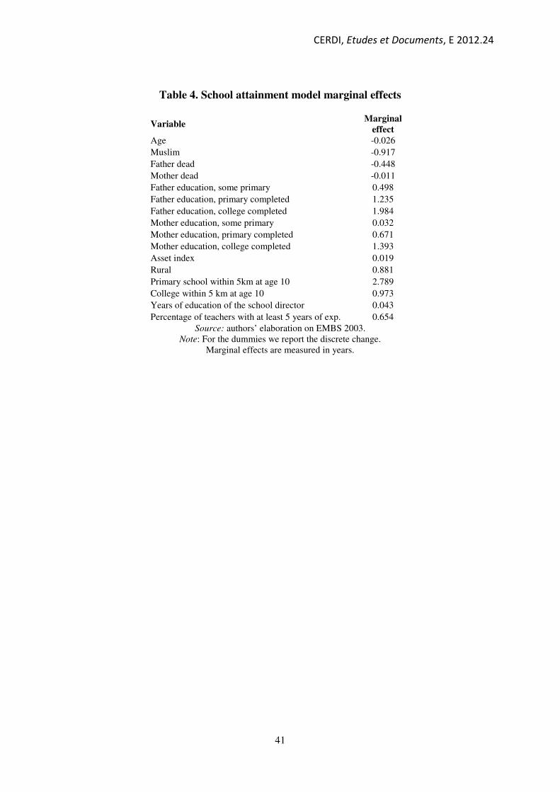
CERDI, Etudes et Documents, E 2012.24
41
Table 4. School attainment model marginal effects
Variable Marginal
effect
Age -0.026
Muslim -0.917
Father dead -0.448
Mother dead -0.011
Father education, some primary 0.498
Father education, primary completed 1.235
Father education, college completed 1.984
Mother education, some primary 0.032
Mother education, primary completed 0.671
Mother education, college completed 1.393
Asset index 0.019
Rural 0.881
Primary school within 5km at age 10 2.789
College within 5 km at age 10 0.973
Years of education of the school director 0.043
Percentage of teachers with at least 5 years of exp. 0.654
Source: authors’ elaboration on EMBS 2003.
Note: For the dummies we report the discrete change.
Marginal effects are measured in years.

CERDI, Etudes et Documents, E 2012.24
42
Table 5: Marginal effects of hazard models
Variable Age at
Marriage
Age at first
child
Age at
entry in
labor
market
Grade (1 standard deviation=3.5 additional
grades) 2.22 1.28 -0.42
Father dead (from 0 to 1) -0.08 -0.66 -1.16
Mother dead (from 0 to 1) -1.89 -1.51 -1.88
Father has primary education
(compared to no education) 1.06 0.76 -3.33
Mother has primary education
(compared to no education) 4.01 1.80 -1.54
Age (1 additional year) -0.43 -0.24 0.3
Ratio of men to women in the cohort
(1 Standard deviation=.132) -1.71 -0.88 0.39
Years condoms were first available
(1 Standard deviation=7.33 years) 0.44 0.05
Availability of condoms in community
(from 0 to 1) 0.81 0.0
Delaying Marriage (1 year) 0.61 -0.31
Source: authors’ elaboration on EMBS 2003.
Note: effects are measured in years.

CERDI, Etudes et Documents, E 2012.24
43
Table 6: Models with and without heterogeneity
Model with heterogeneity
Model without heterogeneity
Coefficient St error Coefficient St error
Marriage model
Education grade completed -0.138 *** 0.03 -0.128 *** 0.02
Parenthood model
Marriage duration spline, intercept 1.555 *** 0.24 1.941 *** 0.22
Marriage duration 0-3 years 0.960 *** 0.12 0.961 *** 0.11
Marriage duration 3+ years 0.078 0.07 0.115 * 0.06
Education grade completed -0.033 0.05 -0.047* 0.03
Labor Market model
Marriage duration spline, intercept 0.547 * 0.29 -0.559** 0.28
Marriage duration 0-3 years -0.373 ** 0.17 -0.396** 0.17
Marriage duration 3+ years -0.035 0.08 -0.050 0.08
Motherhood duration spline, intercept -0.118 0.74 -0.041 0.74
Motherhood duration, 0-2 years -0.352 0.90 -0.305 0.89
Motherhood duration, 2+ years 0.039 0.07 0.066 0.07
Education grade completed 0.007 0.04 0.003 0.03
Log Likelihood -12163.75 -12176.06
Source: authors’ elaboration on EMBS 2003.

CERDI, Etudes et Documents, E 2012.24
44
Figure 1. Survival Function of marriage and parenthood
0.2
.4.6
.81
5 10 15 20 25 30Age
Survival function, parenthood Survival function, marriage

CERDI, Etudes et Documents, E 2012.24
45
Figure 2. Survival function for parenthood, delaying marriage by 1 year
0.2
.4.6
.81
5 10 15 20 25 30Age
Survival function, parenthood Survival, delaying marriage

CERDI, Etudes et Documents, E 2012.24
46
Figure 3. Survival function of labor market entry, increasing grades of 1 standard
deviation
.85
.9.9
51
5 10 15 20 25 30Age
Survival function, labor Survival, 3.5 additional grades