The role of driving factors in historical and projected

The role of driving factors in historical and projected carbondynamics of upland ecosystems in Alaska

H�EL�ENE GENET,1,14 YUJIE HE,2 ZHOU LYU,2 A. DAVID MCGUIRE,3 QIANLAI ZHUANG,2 JOYCLEIN,1 DAVID D’AMORE,4

ALEC BENNETT,5 AMY BREEN,5 FRANCES BILES,4 EUG�ENIE S. EUSKIRCHEN,1 KRISTOFER JOHNSON,6 TOM KURKOWSKI,5

SVETLANA (KUSHCH) SCHRODER,7 NEAL PASTICK,8,9 T. SCOTT RUPP,5 BRUCE WYLIE,10 YUJIN ZHANG,11

XIAOPING ZHOU,12 AND ZHILIANG ZHU13

1Institute of Arctic Biology, University of Alaska Fairbanks, Fairbanks, Alaska 99775 USA2Earth, Atmospheric, and Planetary Sciences, Purdue University, West Lafayette, Indiana 47907 USA

3U.S. Geological Survey, Alaska Cooperative Fish and Wildlife Research Unit, University of Alaska Fairbanks,Fairbanks, Alaska 99775 USA

4U.S. Department of Agriculture, Forest Service, Pacific Northwest Research Station, Juneau, Alaska 99801 USA5Scenarios Network for Alaska and Arctic Planning, International Arctic Research Center, University of Alaska Fairbanks,

Fairbanks, Alaska 99775 USA6U.S. Department of Agriculture, Forest Service, Northern Research Station, Newtown Square, Pennsylvania 19073 USA

7School of Environmental and Forest Sciences, University of Washington, Seattle, Washington 98195 USA8Stinger Ghaffarian Technologies Inc., contractor to the U.S. Geological Survey, Sioux Falls, South Dakota 57198 USA

9Department of Forest Resources, University of Minnesota, St. Paul, Minnesota 55108 USA10U.S. Geological Survey, The Earth Resources Observation Systems Center, Sioux Falls, South Dakota 57198 USA

11Chinese Academy of Sciences, Beijing,, China12U.S. Department of Agriculture, Forest Service, Pacific Northwest Research Station, Portland, Oregon 97208 USA

13U.S. Geological Survey, Reston, Virginia 12201 USA

Abstract. It is important to understand how upland ecosystems of Alaska, which are esti-mated to occupy 84% of the state (i.e., 1,237,774 km2), are influencing and will influence state-wide carbon (C) dynamics in the face of ongoing climate change. We coupled fire disturbanceand biogeochemical models to assess the relative effects of changing atmospheric carbon diox-ide (CO2), climate, logging and fire regimes on the historical and future C balance of uplandecosystems for the four main Landscape Conservation Cooperatives (LCCs) of Alaska. At theend of the historical period (1950–2009) of our analysis, we estimate that upland ecosystems ofAlaska store ~50 Pg C (with ~90% of the C in soils), and gained 3.26 Tg C/yr. Three of theLCCs had gains in total ecosystem C storage, while the Northwest Boreal LCC lost C(�6.01 Tg C/yr) because of increases in fire activity. Carbon exports from logging affected onlythe North Pacific LCC and represented less than 1% of the state’s net primary production(NPP). The analysis for the future time period (2010–2099) consisted of six simulations drivenby climate outputs from two climate models for three emission scenarios. Across the climatescenarios, total ecosystem C storage increased between 19.5 and 66.3 Tg C/yr, which represents3.4% to 11.7% increase in Alaska upland’s storage. We conducted additional simulations toattribute these responses to environmental changes. This analysis showed that atmosphericCO2 fertilization was the main driver of ecosystem C balance. By comparing future simulationswith constant and with increasing atmospheric CO2, we estimated that the sensitivity of NPPwas 4.8% per 100 ppmv, but NPP becomes less sensitive to CO2 increase throughout the 21stcentury. Overall, our analyses suggest that the decreasing CO2 sensitivity of NPP and theincreasing sensitivity of heterotrophic respiration to air temperature, in addition to the increasein C loss from wildfires weakens the C sink from upland ecosystems of Alaska and willultimately lead to a source of CO2 to the atmosphere beyond 2100. Therefore, we concludethat the increasing regional C sink we estimate for the 21st century will most likely betransitional.

Key words: Alaska carbon cycle; atmospheric CO2; carbon balance; climate change; fire; logging;permafrost; soil carbon; upland ecosystem; vegetation productivity.

Manuscript received 6 April 2017; revised 26 July 2017; accepted 25 August 2017. Corresponding Editor: Yude Pan.Editors’ Note: Papers in Invited Features are published individually and are linked online in a virtual table of contents on the

journal website.14 E-mail: [email protected]

1

INVITED FEATURE ARTICLE

Ecological Applications, 0(0), 2017, pp. 1–23© 2017 by the Ecological Society of America

INTRODUCTION

The design of efficient policies to mitigate climatechange relies on robust predictions of how the carbon(C) balance of terrestrial ecosystems will respond to dif-ferent pathways of climate change. Because of the largeamount of C stored in northern high latitude ecosystems(Schuur et al. 2015), pathways of climate change couldbe altered by responses of C balance in this region(McGuire et al. 2012). Recent estimate of C stored inpermafrost soils (0–3 m) of Arctic and sub-Arcticregions are 1,035 Pg C (�150 Pg C 95% confidenceinterval; Michaelson et al. 2013, Hugelius et al. 2013,2014). Because of polar amplification, the rate of warm-ing in the Arctic has been 1.6 times higher than the ratein lower latitudes between 1875 and 2008 (Bekryaevet al. 2010). Climate warming is altering a range of bio-logical and physical processes, including those related topermafrost dynamics and hydrology (Romanovsky et al.2010, Liljedahl et al. 2016), vegetation composition andproductivity (Stow et al. 2004, Beck and Goetz 2011,Myers-Smith et al. 2011) and disturbance regimes suchas wildfire (Kasischke and Turetsky 2006, De Grootet al. 2013) and thermokarst (Jorgenson et al. 2001,Lara et al. 2016, Nitze and Grosse 2016). These changesmay trigger profound transitions in ecosystem trajecto-ries (Hinzman et al. 2013) that will affect C sequestra-tion and C dynamics at local and regional scales.Increases in vegetation productivity from rising atmo-

spheric carbon dioxide (CO2) and air temperature arewell documented (Ainsworth and Long 2005, Chapinet al. 2006, Zeng et al. 2011, Bieniek et al. 2015) andcan enhance C sequestration in the soil by increasing Cinput from litterfall (Harden et al. 1992, Yuan et al.2012). This enhanced C uptake may be partially orwholly offset by C releases to the atmosphere fromincreases in decomposition and fire emissions in arcticand boreal ecosystems (Hayes et al. 2011). Permafrostthaw driven by climate warming exposes deep soil C towarmer temperatures that can increase decomposition,and ultimately release soil organic C (SOC) to the atmo-sphere in the form of CO2 or methane (CH4), dependingon the local drainage conditions (Harden et al. 2006,2012a,b, Schuur et al. 2008, Hugelius et al. 2013). Addi-tionally, increases in air temperature may lead to anincrease in fire frequency and severity (Kasischke et al.2002, Balshi et al. 2009) that could cause further warm-ing through (1) large pyrogenic C releases to the atmo-sphere (Turetsky et al. 2011, Genet et al. 2013), (2)decreasing photosynthetic activity from fire-killed vege-tation (Goetz et al. 2007), and (3) further thawing of thepermafrost through combustion of the insulatingorganic layer (Jafarov et al. 2013, Johnson et al. 2013,Jones et al. 2015). A recent synthesis has estimated thatbetween 130 and 160 Pg C could be released from soilsof the northern permafrost region to the atmosphereduring the 21st century under the current warming tra-jectory given no changes in productivity (Schuur et al.

2015). In addition, it has been estimated that C emis-sions from wildfire could increase fourfold compared tohistorical emissions (Abbott et al. 2016). Finally, com-mercial timber harvest in boreal and coastal forests mayimpact regional C balance by exporting significant Cstocks out of terrestrial ecosystems, and affecting standage distribution (Cole et al. 2010).The state of Alaska contains ~7% of the global tundra

biome extent (CAVM Team 2003), ~4% of the boreal for-est biome extent (Whittaker 1975), and ~5% of the extentof permafrost regions (Brown et al. 1998). Alaska alsoexperiences substantial fire activity (Kasischke et al.2010), and a large proportion of its landscape is under-lain by permafrost vulnerable to significant thaw over the21st century (Pastick et al. 2017), which would exposepreviously protected C stocks to decomposition underprojected climate change (Turetsky et al. 2011, Hayeset al. 2014). However, spatial and temporal dynamics offire and thawing permafrost are shaped by landform anddrainage conditions. In Alaska, uplands are estimated tooccupy 84% of the landscape (Pastick et al. 2017). Com-pared to lowlands (i.e., wetlands and peatlands), uplandsare characterized by better drainage conditions with aer-obic soils that promote relatively high rates of decompo-sition that primarily produce CO2 (Schuur et al. 2008).Methanogenesis is limited in well-drained soils and CH4

production can be offset by methanotrophy (Whalen andReeburgh 1990). Low moisture content and more flam-mable fuel load are associated with higher frequency ofwildfire in well drained uplands compared to poorlydrained lowlands (Turetsky et al. 2011, Genet et al.2013). Additionally, shallow and dry organic layer andfrequent wildfire contribute to a lower resilience of per-mafrost to climate change compared to poorly drainedlowlands with lower fire frequency (Jafarov et al. 2013,Johnson et al. 2013). Finally, commercial timber harvestin Alaska occurs mainly in upland maritime forests ofsoutheastern coastal Alaska (i.e., western hemlock [Tsugaheterophylla (Raf.) Sarg.] and Sitka spruce [Picea sitchen-sis (Bong.) Carri�ere] forests). On the other hand, morerapid nutrient cycling and deep rooting occur in well-drained upland ecosystems, which are expected to lead tohigher vegetation productivity than lowland ecosystems(Bhatti et al. 2010). Because processes affecting C bal-ance have different sensitivities to climate change, it isimportant to explicitly separate uplands from lowlandsin regional assessments of C dynamics to climate change.This study is focused on C dynamics in uplands ofAlaska. Lowland C dynamics of Alaska are the focus ofa separate paper in this invited feature (Lyu et al. 2016).The main goal of this study is to provide an assess-

ment of the historical and future trajectory of C dynam-ics in upland ecosystems of Alaska and to diagnose themechanisms responsible for these dynamics. To achievethis goal, we applied a modeling framework that hasbeen designed and calibrated to represent major vegeta-tion communities of upland ecosystems in arctic, borealand maritime regions of Alaska. We made use of recent

2 H�EL�ENE GENET ET AL.Ecological Applications

Vol. 0, No. 0

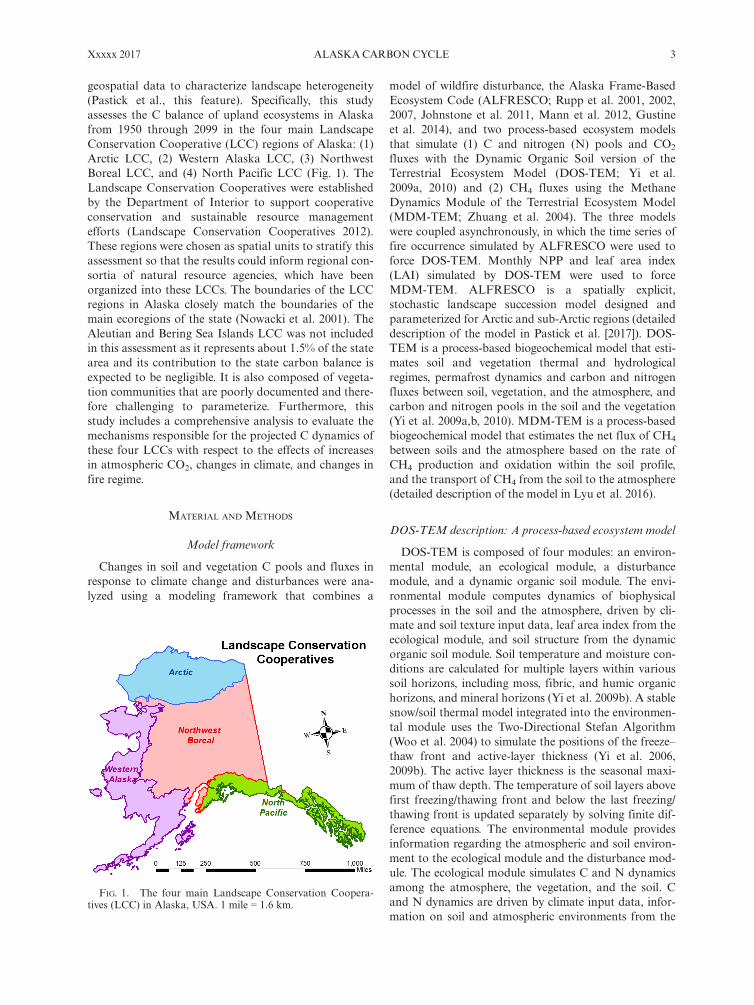
geospatial data to characterize landscape heterogeneity(Pastick et al., this feature). Specifically, this studyassesses the C balance of upland ecosystems in Alaskafrom 1950 through 2099 in the four main LandscapeConservation Cooperative (LCC) regions of Alaska: (1)Arctic LCC, (2) Western Alaska LCC, (3) NorthwestBoreal LCC, and (4) North Pacific LCC (Fig. 1). TheLandscape Conservation Cooperatives were establishedby the Department of Interior to support cooperativeconservation and sustainable resource managementefforts (Landscape Conservation Cooperatives 2012).These regions were chosen as spatial units to stratify thisassessment so that the results could inform regional con-sortia of natural resource agencies, which have beenorganized into these LCCs. The boundaries of the LCCregions in Alaska closely match the boundaries of themain ecoregions of the state (Nowacki et al. 2001). TheAleutian and Bering Sea Islands LCC was not includedin this assessment as it represents about 1.5% of the statearea and its contribution to the state carbon balance isexpected to be negligible. It is also composed of vegeta-tion communities that are poorly documented and there-fore challenging to parameterize. Furthermore, thisstudy includes a comprehensive analysis to evaluate themechanisms responsible for the projected C dynamics ofthese four LCCs with respect to the effects of increasesin atmospheric CO2, changes in climate, and changes infire regime.

MATERIAL AND METHODS

Model framework

Changes in soil and vegetation C pools and fluxes inresponse to climate change and disturbances were ana-lyzed using a modeling framework that combines a

model of wildfire disturbance, the Alaska Frame-BasedEcosystem Code (ALFRESCO; Rupp et al. 2001, 2002,2007, Johnstone et al. 2011, Mann et al. 2012, Gustineet al. 2014), and two process-based ecosystem modelsthat simulate (1) C and nitrogen (N) pools and CO2

fluxes with the Dynamic Organic Soil version of theTerrestrial Ecosystem Model (DOS-TEM; Yi et al.2009a, 2010) and (2) CH4 fluxes using the MethaneDynamics Module of the Terrestrial Ecosystem Model(MDM-TEM; Zhuang et al. 2004). The three modelswere coupled asynchronously, in which the time series offire occurrence simulated by ALFRESCO were used toforce DOS-TEM. Monthly NPP and leaf area index(LAI) simulated by DOS-TEM were used to forceMDM-TEM. ALFRESCO is a spatially explicit,stochastic landscape succession model designed andparameterized for Arctic and sub-Arctic regions (detaileddescription of the model in Pastick et al. [2017]). DOS-TEM is a process-based biogeochemical model that esti-mates soil and vegetation thermal and hydrologicalregimes, permafrost dynamics and carbon and nitrogenfluxes between soil, vegetation, and the atmosphere, andcarbon and nitrogen pools in the soil and the vegetation(Yi et al. 2009a,b, 2010). MDM-TEM is a process-basedbiogeochemical model that estimates the net flux of CH4

between soils and the atmosphere based on the rate ofCH4 production and oxidation within the soil profile,and the transport of CH4 from the soil to the atmosphere(detailed description of the model in Lyu et al. 2016).

DOS-TEM description: A process-based ecosystem model

DOS-TEM is composed of four modules: an environ-mental module, an ecological module, a disturbancemodule, and a dynamic organic soil module. The envi-ronmental module computes dynamics of biophysicalprocesses in the soil and the atmosphere, driven by cli-mate and soil texture input data, leaf area index from theecological module, and soil structure from the dynamicorganic soil module. Soil temperature and moisture con-ditions are calculated for multiple layers within varioussoil horizons, including moss, fibric, and humic organichorizons, and mineral horizons (Yi et al. 2009b). A stablesnow/soil thermal model integrated into the environmen-tal module uses the Two-Directional Stefan Algorithm(Woo et al. 2004) to simulate the positions of the freeze–thaw front and active-layer thickness (Yi et al. 2006,2009b). The active layer thickness is the seasonal maxi-mum of thaw depth. The temperature of soil layers abovefirst freezing/thawing front and below the last freezing/thawing front is updated separately by solving finite dif-ference equations. The environmental module providesinformation regarding the atmospheric and soil environ-ment to the ecological module and the disturbance mod-ule. The ecological module simulates C and N dynamicsamong the atmosphere, the vegetation, and the soil. Cand N dynamics are driven by climate input data, infor-mation on soil and atmospheric environments from the

FIG. 1. The four main Landscape Conservation Coopera-tives (LCC) in Alaska, USA. 1 mile = 1.6 km.

Xxxxx 2017 ALASKACARBON CYCLE 3

environmental module, information on soil structure pro-vided by the dynamic organic soil module, and informa-tion on timing and severity of wildfire or forest harvestprovided by the disturbance module. DOS-TEM simu-lates the dynamics of three different soil C horizons (thefibrous, amorphous, and mineral soil horizons), and Cand N dynamics in the aboveground and belowgroundcompartments of the vegetation. The C from litterfall isdivided into aboveground and belowground litterfall.Aboveground litterfall is assigned only to the first layerof the fibrous horizon, while belowground litterfall isassigned to different layers of the three soil horizonsbased on the fractional distribution of fine roots withdepth. The dynamic organic soil module calculates thethickness of the fibric and sapric/humic organic horizonsafter soil C pools are altered by ecological processes(litterfall, decomposition, and burial) and fire distur-bance. The estimation of organic horizon thickness iscomputed from soil C content using relationships thatlink soil organic C content and soil organic thickness(i.e., pedotransfer functions; Yi et al. 2009a). These rela-tionships have been developed for fibric, sapric/humic,and mineral horizons for every vegetation type, based ondata from the soil C network database for Alaska (John-son et al. 2011). Finally, the disturbance module simu-lates how forest harvest and wildfire affects stand agedistribution C and N pools of the vegetation and the soil.For wildfire, the module computes combustion emissionsto the atmosphere, the fate of uncombusted C and Npools, and the flux of N from the atmosphere to the soilvia biological N fixation in the years following fire. Therates of combustion of the organic layer and the mortal-ity rate in the vegetation depend on fire severity. In bor-eal forest, fire severity is determined using input data ontopography, drainage, and vegetation, as well as soil(moisture and temperature) and atmospheric (evapotran-spiration) environmental data from the environmentalmodule (Genet et al. 2013). In tundra, the rates of com-bustion and vegetation mortality are based on those esti-mated from the 2007 Anaktuvuk River Fire (Mack et al.2011). Methane emissions from fire were estimated a pos-teriori by applying an emission factor as estimated byFrench et al. (2002) to the fire emissions simulated byDOS-TEM. The effects of forest harvest disturbance onC and N balances are also included in the disturbancemodule. Commercial timber harvest by clear-cutting hasbeen widespread in southeastern Alaska since the early1950s (Alaback 1982, Cole et al. 2010). We developed aharvesting function with the assumption that 95% of theaboveground vegetation biomass within a logged stand isharvested (Deal and Tappeiner 2002). Among the resid-ual biomass, 4% was considered dead and 1% alive toallow post-harvest recruitment. As a consequence, 99%of the root vegetation biomass was considered dead andtransferred to the soil organic matter pool.Regional applications of versions of TEM that lead to

DOS-TEM in northern high latitudes have investigatedhow biogeochemical dynamics of terrestrial ecosystems

are affected at seasonal to century scales by processeslike permafrost thaw and soil thermal dynamics (Zhuanget al. 2002, 2003, Euskirchen et al. 2006), snow cover(Euskirchen et al. 2006, 2007), and warming and fire dis-turbance (Balshi et al. 2007, Sitch et al. 2007).

DOS-TEM parameterization and validation

Rate-limiting parameters of the model were calibratedfor eight main upland land-cover types in Alaska: threetypes of tundra (graminoid, shrub, heath), three types ofboreal upland forest (black spruce [Picea mariana (Mill.)Britton, Sterns & Poggenb.], white spruce [Picea glauca(Moench) Voss], and deciduous forest), and two types ofupland maritime communities (upland Maritime forestand alder shrubland). A detailed description of theseland-cover types is available in Pastick et al. (2017).For each upland land cover type, the rate-limiting

parameters of DOS-TEM were calibrated to target val-ues of C and N pools and fluxes representative of matureecosystems (Clein et al. 2002, see list in target variablesin Appendix S1). The calibration of these parameters isan effective means of dealing with temporal scaling issuesin ecosystem models (Rastetter et al. 1992). For borealforest communities, an existing set of target values forvegetation and soil C and N pools and fluxes was assem-bled using data collected in the Bonanza Creek LongTerm Ecological Research program (LTER; Yuan et al.2012), updated with data from the most recent version ofthe Bonanza Creek LTER database. For the tundra com-munities, we used data collected near the Toolik FieldStation as part of the Arctic LTER program (Shaver andChapin 1991, Van Wijk et al. 2003, Sullivan et al. 2007,Euskirchen et al. 2012, Gough et al. 2012, Sistla et al.2013). Finally, for the maritime upland forest, we useddata collected from a long-term C flux study in the NorthAmerican Carbon Program (D’Amore et al. 2012). Thetarget values for maritime alder shrubland were assem-bled from Binkley (1982). The target values used for allof these calibrations are listed in Appendix S1.The DOS-TEM parameterizations were validated using

soil and vegetation biomass data derived from field obser-vations independent of the data used for model calibra-tion. The validation analysis for DOS-TEM is presentedin Genet et al. (2016). The National Soil Carbon Net-work database for Alaska (Johnson et al. 2011) was usedto validate DOS-TEM estimates of soil C pools. To com-pare similar estimates from the model and observations,only deep profiles were selected from the database, i.e.,profiles with a description of the entire organic horizonsand 90 to 110 cm thick mineral horizon below theorganic horizons. Estimates of vegetation C pools for tun-dra land-cover types were compared with observationsrecorded in the data catalog of the Arctic LTER at ToolikField Station. For boreal forest land-cover types, vegeta-tion C pools simulated by DOS-TEM were comparedwith estimates from forest inventories conducted by theCooperative Alaska Forest Inventory Program (Malone


Vol. 0, No. 0

et al. 2009). The forest inventory only provided estimatesof aboveground biomass. Aboveground biomass was con-verted to total biomass by using a ratio of abovegroundvs. total biomass of 0.8 in forest (Ruess et al. 1996) and0.6 in tundra land-cover types (Gough et al. 2012). Thecontent of C in biomass was estimated at 50%. Finally,for the land-cover types of southeastern coastal Alaska(that is, the North Pacific LCC maritime upland forestand alder shrubland), model validation was not possibleas no additional independent data were available in thisregion (the plot coordinates of the Forest Inventory ofAlaska not being available, site specific comparisons werenot possible). For these land-cover types, we comparedthe model simulations with observed data on the samesites that were used for model parameterization. No sig-nificant differences were observed between modeled andobserved contemporary vegetation and soil C stocks(P values of 0.340 and 0.085, respectively). Additionally,DOS-TEM simulations successfully reproduced differ-ences between land-cover types.

Model application

The distribution of uplands in Alaska was assessedfrom a new, 1-km resolution, wetland map for Alaskaidentifying upland, fen, bogs, and open waters. The wet-land map was developed using the Alaska National Wet-lands Inventory as a reference data set (availableonline).15 This map is described in detail by Pastick et al.(2017). Uplands in Alaska are estimated to cover1,237,775 km2, which represents about 84% of the areaof the state. The upland vegetation communities wereidentified using a baseline land cover map derived fromthe 2005 map from the North America Land CoverMonitoring System (Natural Resources Canada/Cana-dian Center for Remote Sensing [NRCan/CCRS] et al.2005).Simulations were conducted across Alaska at a 1-km

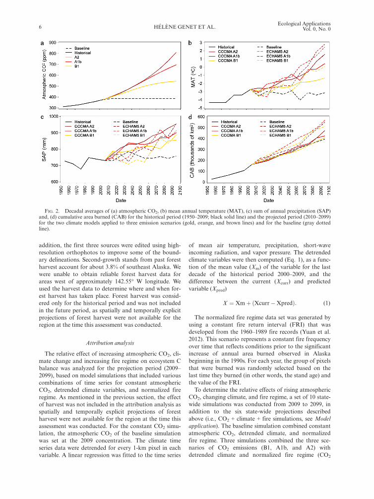
resolution from 1950 through 2099. DOS-TEM is drivenby annual atmospheric CO2 concentration, monthlymean air temperature, total precipitation, net incomingshortwave radiation, and vapor pressure. The atmo-spheric CO2 and climate projections were aligned withthe Intergovernmental Panel on Climate Change’s Spe-cial Report on Emission Scenarios (IPCC-SRES; Naki-cenovic et al. 2000). The assessment was driven by threeCO2 concentration trajectories associated with low-,mid- and high-range CO2 emission scenarios (A1b, A2,and B1, respectively; Fig. 2a).Before conducting the transient simulations, a typical

spin-up procedure was conducted for each spatial loca-tion in which the model was driven by averaged modernforcings for that location, repeated continuously untildynamic equilibrium was achieved (i.e., constant poolsand fluxes at that location). The resulting modelledecosystem state for each spatial location then served as

the starting point for the transient simulation during thehistorical and future periods presented in this study.To evaluate the effects of historical and projected cli-

mate warming, simulations were driven by output fromtwo climate models for each of the three emission scenar-ios (Fig. 2b, c). Each of the six climate scenarios utilizedthe same downscaled historical climate data from 1901through 2009 from the Climatic Research Unit (CRU TS3.1; Harris et al. 2014). The climate projections weredeveloped for 2010 through 2099 from the outputs of (1)version 3.1-T47 of the Coupled Global Climate Model(CGCM3.1; McFarlane et al. 1992) developed by theCanadian Centre for Climate Modelling and Analysisand (2) version 5 of the European Centre HamburgModel (ECHAM5; Roeckner et al. 2004) developed bythe Max Planck Institute (models available online.16,17

Additional methodological details for the downscaled cli-mate variables can be found in Pastick et al. (2017).The fire occurrence data set combined (1) historical

records from 1950 through 2009 obtained from the AlaskaInteragency Coordination Center large fire scar database(Kasischke et al. 2002; database available online)18 and (2)projected scenarios from ALFRESCO (Pastick et al.2017). These scenarios represent the anticipated changesin fire frequency in response to climate change, and result-ing changes in vegetation composition over time due tofire disturbance and secondary succession (Fig. 2d).ALFRESCO produces an ensemble of simulations(n = 200) for each climate scenario to represent the uncer-tainty of the response of fire regime to climate. ReplicatingDOS-TEM simulations across the region for each scenariowould have been impractical as these simulations are com-putationally intensive. Subsequently, for each climate sce-nario, the fire time series selected to run DOS-TEMsimulations were the simulation that best reproduced his-torical fire records in terms of annual area burned andmean fire size. Topographic information from theNational Elevation Dataset of the U.S. Geological Surveyat 60-m resolution (NED) was used to calculate fire sever-ity with the algorithm of Genet et al. (2013); NED avail-able online .19 The topographic descriptors included slope,aspect, and log-transformed flow accumulation.Historical records of forest harvest area from 1950

through 2009 in southeast and south-central Alaskawere compiled from geographic information system datafrom four different sources: (1) the USDA Forest Ser-vice, Tongass National Forest; (2) the Nature Conser-vancy’s past harvest repository; (3) the State of AlaskaDepartment of Natural Resources; and (4) screen digi-tizing from high-resolution orthophotos of some har-vests not included in the previously listed sources. In

15 http://www.fws.gov/wetlands/Data/State-Downloads.html

16 https://www.canada.ca/en/environment-climate-change/services/climate-change/centre-modelling-analysis/models/third-generation-coupled-global.html

17 https://www.mpimet.mpg.de/en/science/models/mpi-esm/18 http://fire.ak.blm.gov/19 http://ned.usgs.gov/


http://www.fws.gov/wetlands/Data/State-Downloads.html

https://www.canada.ca/en/environment-climate-change/services/climate-change/centre-modelling-analysis/models/third-generation-coupled-global.html



https://www.mpimet.mpg.de/en/science/models/mpi-esm/

http://fire.ak.blm.gov/

http://ned.usgs.gov/

addition, the first three sources were edited using high-resolution orthophotos to improve some of the bound-ary delineations. Second-growth stands from past forestharvest account for about 3.8% of southeast Alaska. Wewere unable to obtain reliable forest harvest data forareas west of approximately 142.55° W longitude. Weused the harvest data to determine where and when for-est harvest has taken place. Forest harvest was consid-ered only for the historical period and was not includedin the future period, as spatially and temporally explicitprojections of forest harvest were not available for theregion at the time this assessment was conducted.

Attribution analysis

The relative effect of increasing atmospheric CO2, cli-mate change and increasing fire regime on ecosystem Cbalance was analyzed for the projection period (2009–2099), based on model simulations that included variouscombinations of time series for constant atmosphericCO2, detrended climate variables, and normalized fireregime. As mentioned in the previous section, the effectof harvest was not included in the attribution analysis asspatially and temporally explicit projections of forestharvest were not available for the region at the time thisassessment was conducted. For the constant CO2 simu-lation, the atmospheric CO2 of the baseline simulationwas set at the 2009 concentration. The climate timeseries data were detrended for every 1-km pixel in eachvariable. A linear regression was fitted to the time series

of mean air temperature, precipitation, short-waveincoming radiation, and vapor pressure. The detrendedclimate variables were then computed (Eq. 1), as a func-tion of the mean value (Xm) of the variable for the lastdecade of the historical period 2000–2009, and thedifference between the current (Xcurr) and predictedvariable (Xpred)

X ¼ Xmþ ðXcurr�XpredÞ: (1)

The normalized fire regime data set was generated byusing a constant fire return interval (FRI) that wasdeveloped from the 1960–1989 fire records (Yuan et al.2012). This scenario represents a constant fire frequencyover time that reflects conditions prior to the significantincrease of annual area burned observed in Alaskabeginning in the 1990s. For each year, the group of pixelsthat were burned was randomly selected based on thelast time they burned (in other words, the stand age) andthe value of the FRI.To determine the relative effects of rising atmospheric

CO2, changing climate, and fire regime, a set of 10 state-wide simulations was conducted from 2009 to 2099, inaddition to the six state-wide projections describedabove (i.e., CO2 + climate + fire simulations, see Modelapplication). The baseline simulation combined constantatmospheric CO2, detrended climate, and normalizedfire regime. Three simulations combined the three sce-narios of CO2 emissions (B1, A1b, and A2) withdetrended climate and normalized fire regime (CO2

FIG. 2. Decadal averages of (a) atmospheric CO2, (b) mean annual temperature (MAT), (c) sum of annual precipitation (SAP)and, (d) cumulative area burned (CAB) for the historical period (1950–2009; black solid line) and the projected period (2010–2099)for the two climate models applied to three emission scenarios (gold, orange, and brown lines) and for the baseline (gray dottedline).


Vol. 0, No. 0

simulations). Finally, six simulations were conductedwith rising atmospheric CO2, and the six climate model-scenarios and normalized fire regime (CO2 + climatesimulations). The effect of CO2 fertilization was esti-mated by comparing baseline simulations with the CO2

simulations. The effect of climate change was estimatedby comparing decadal averages from the CO2 simula-tions with the decadal averages from the CO2 + climatesimulations. Finally, the effect of a changing fire regimewas estimated by comparing the CO2 + climate simula-tions with the CO2 + climate + fire simulations.

Assessing ecosystem C balance

Vegetation C stock estimates were derived from thesum of aboveground and belowground living biomass.Soil C pools were composed of C stored in the deadwoody debris fallen to the ground, moss and litter,organic layers and mineral layers. Historical changes insoil and vegetation C pools were evaluated by quantify-ing cumulative changes from the estimate of the respec-tive C pool at the end of 1949. Projected changes in soiland vegetation C pools were evaluated by quantifyingcumulative changes from the estimate of the respective Cpool at the end of 2009.The net ecosystem carbon balance (NECB) is the dif-

ference between total C inputs and total C outputs to theecosystem (Chapin et al. 2006). NECB is the sum of allC fluxes coming in and out of the ecosystems, throughgaseous and nongaseous, dissolved and non-dissolvedexchanges with the atmosphere and the hydrologicnetwork. In the present study, the C exchange betweenterrestrial and aquatic ecosystems are not considered. Interrestrial ecosystems, NECB (Eq. 2) is the sum of netprimary productivity (NPP) and net biogenic methaneflux (BioCH4) minus heterotrophic respiration (HR), fireemissions (Fire), and forest harvest exports (Harvest, forthe historical simulation only)

NECB ¼ NPPþ BioCH4 �HR� Fire�Harvest: (2)

NPP results from C assimilation from vegetation pho-tosynthesis minus the respiration of the primary produc-ers (autotrophic respiration). The activity of soilmethanotrophs dominates the methane cycle in uplands.For this reason, BioCH4 is a positive net flux from theatmosphere into upland ecosystems. HR results from thedecomposition of unfrozen SOC. Fire emissions includeC from CO2, CH4, and carbon monoxide (CO) emis-sions. Forest harvest quantifies the amount of vegetationC that is exported out of the terrestrial ecosystem to thewood products sector. Positive NECB indicates a gain ofC to the ecosystem from the atmosphere (C sink), andnegative NECB indicates a loss of C from the ecosystemto the atmosphere and harvested wood product pool (Csource). Uncertainty of NECB associated with the cli-mate scenarios was quantified by the standard deviationamong the six tested scenarios of mean NECB for the

last decade of the 21st century (i.e., CO2 + climate + firesimulations).

Statistical analysis of the environmental drivers ofecosystem C balance

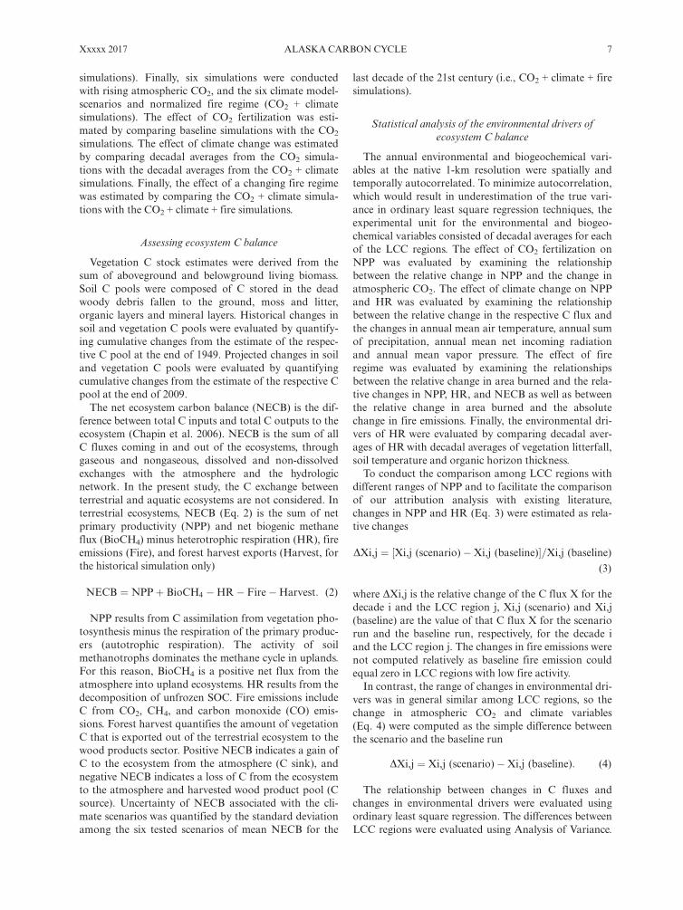
The annual environmental and biogeochemical vari-ables at the native 1-km resolution were spatially andtemporally autocorrelated. To minimize autocorrelation,which would result in underestimation of the true vari-ance in ordinary least square regression techniques, theexperimental unit for the environmental and biogeo-chemical variables consisted of decadal averages for eachof the LCC regions. The effect of CO2 fertilization onNPP was evaluated by examining the relationshipbetween the relative change in NPP and the change inatmospheric CO2. The effect of climate change on NPPand HR was evaluated by examining the relationshipbetween the relative change in the respective C flux andthe changes in annual mean air temperature, annual sumof precipitation, annual mean net incoming radiationand annual mean vapor pressure. The effect of fireregime was evaluated by examining the relationshipsbetween the relative change in area burned and the rela-tive changes in NPP, HR, and NECB as well as betweenthe relative change in area burned and the absolutechange in fire emissions. Finally, the environmental dri-vers of HR were evaluated by comparing decadal aver-ages of HRwith decadal averages of vegetation litterfall,soil temperature and organic horizon thickness.To conduct the comparison among LCC regions with

different ranges of NPP and to facilitate the comparisonof our attribution analysis with existing literature,changes in NPP and HR (Eq. 3) were estimated as rela-tive changes

DXi,j ¼ ½Xi,j (scenario)�Xi,j (baseline)�=Xi,j (baseline)

(3)

where DXi,j is the relative change of the C flux X for thedecade i and the LCC region j, Xi,j (scenario) and Xi,j(baseline) are the value of that C flux X for the scenariorun and the baseline run, respectively, for the decade iand the LCC region j. The changes in fire emissions werenot computed relatively as baseline fire emission couldequal zero in LCC regions with low fire activity.In contrast, the range of changes in environmental dri-

vers was in general similar among LCC regions, so thechange in atmospheric CO2 and climate variables(Eq. 4) were computed as the simple difference betweenthe scenario and the baseline run

DXi,j ¼ Xi,j (scenario)�Xi,j (baseline): (4)

The relationship between changes in C fluxes andchanges in environmental drivers were evaluated usingordinary least square regression. The differences betweenLCC regions were evaluated using Analysis of Variance.


All analyses were performed using the SAS statisticalpackage (SAS 9.4; SAS Institute, Cary, North Carolina,USA). The assumptions of normality and homoscedas-ticity were verified by examining residual plots. Effectswere considered significant at the 0.05 level. Averages ofC stocks and fluxes are accompanied with the estimatedstandard deviation from annual variations (SD).

RESULTS

Historical C dynamics of upland ecosystems in Alaskafrom 1950 through 2009

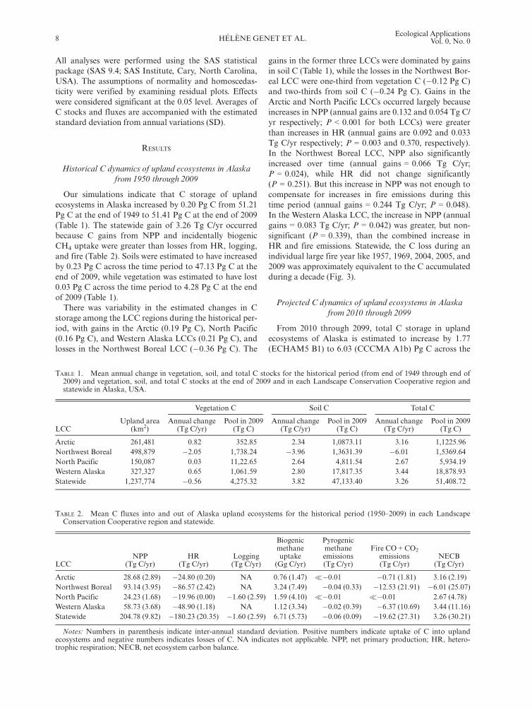
Our simulations indicate that C storage of uplandecosystems in Alaska increased by 0.20 Pg C from 51.21Pg C at the end of 1949 to 51.41 Pg C at the end of 2009(Table 1). The statewide gain of 3.26 Tg C/yr occurredbecause C gains from NPP and incidentally biogenicCH4 uptake were greater than losses from HR, logging,and fire (Table 2). Soils were estimated to have increasedby 0.23 Pg C across the time period to 47.13 Pg C at theend of 2009, while vegetation was estimated to have lost0.03 Pg C across the time period to 4.28 Pg C at the endof 2009 (Table 1).There was variability in the estimated changes in C

storage among the LCC regions during the historical per-iod, with gains in the Arctic (0.19 Pg C), North Pacific(0.16 Pg C), and Western Alaska LCCs (0.21 Pg C), andlosses in the Northwest Boreal LCC (�0.36 Pg C). The

gains in the former three LCCs were dominated by gainsin soil C (Table 1), while the losses in the Northwest Bor-eal LCC were one-third from vegetation C (�0.12 Pg C)and two-thirds from soil C (�0.24 Pg C). Gains in theArctic and North Pacific LCCs occurred largely becauseincreases in NPP (annual gains are 0.132 and 0.054 Tg C/yr respectively; P < 0.001 for both LCCs) were greaterthan increases in HR (annual gains are 0.092 and 0.033Tg C/yr respectively; P = 0.003 and 0.370, respectively).In the Northwest Boreal LCC, NPP also significantlyincreased over time (annual gains = 0.066 Tg C/yr;P = 0.024), while HR did not change significantly(P = 0.251). But this increase in NPP was not enough tocompensate for increases in fire emissions during thistime period (annual gains = 0.244 Tg C/yr; P = 0.048).In the Western Alaska LCC, the increase in NPP (annualgains = 0.083 Tg C/yr; P = 0.042) was greater, but non-significant (P = 0.339), than the combined increase inHR and fire emissions. Statewide, the C loss during anindividual large fire year like 1957, 1969, 2004, 2005, and2009 was approximately equivalent to the C accumulatedduring a decade (Fig. 3).

Projected C dynamics of upland ecosystems in Alaskafrom 2010 through 2099

From 2010 through 2099, total C storage in uplandecosystems of Alaska is estimated to increase by 1.77(ECHAM5 B1) to 6.03 (CCCMA A1b) Pg C across the

TABLE 1. Mean annual change in vegetation, soil, and total C stocks for the historical period (from end of 1949 through end of2009) and vegetation, soil, and total C stocks at the end of 2009 and in each Landscape Conservation Cooperative region andstatewide in Alaska, USA.

Vegetation C Soil C Total C

LCCUpland area

(km2)Annual change

(Tg C/yr)Pool in 2009

(Tg C)Annual change


(Tg C)Annual change


(Tg C)

Arctic 261,481 0.82 352.85 2.34 1,0873.11 3.16 1,1225.96Northwest Boreal 498,879 �2.05 1,738.24 �3.96 1,3631.39 �6.01 1,5369.64North Pacific 150,087 0.03 11,22.65 2.64 4,811.54 2.67 5,934.19Western Alaska 327,327 0.65 1,061.59 2.80 17,817.35 3.44 18,878.93Statewide 1,237,774 �0.56 4,275.32 3.82 47,133.40 3.26 51,408.72

TABLE 2. Mean C fluxes into and out of Alaska upland ecosystems for the historical period (1950–2009) in each LandscapeConservation Cooperative region and statewide.

LCCNPP

(Tg C/yr)HR

(Tg C/yr)Logging(Tg C/yr)

Biogenicmethaneuptake

(Gg C/yr)

Pyrogenicmethaneemissions(Tg C/yr)

Fire CO + CO2emissions(Tg C/yr)

NECB(Tg C/yr)

Arctic 28.68 (2.89) �24.80 (0.20) NA 0.76 (1.47) ��0.01 �0.71 (1.81) 3.16 (2.19)Northwest Boreal 93.14 (3.95) �86.57 (2.42) NA 3.24 (7.49) �0.04 (0.33) �12.53 (21.91) �6.01 (25.07)North Pacific 24.23 (1.68) �19.96 (0.00) �1.60 (2.59) 1.59 (4.10) ��0.01 ��0.01 2.67 (4.78)Western Alaska 58.73 (3.68) �48.90 (1.18) NA 1.12 (3.34) �0.02 (0.39) �6.37 (10.69) 3.44 (11.16)Statewide 204.78 (9.82) �180.23 (20.35) �1.60 (2.59) 6.71 (5.73) �0.06 (0.09) �19.62 (27.31) 3.26 (30.21)

Notes: Numbers in parenthesis indicate inter-annual standard deviation. Positive numbers indicate uptake of C into uplandecosystems and negative numbers indicates losses of C. NA indicates not applicable. NPP, net primary production; HR, hetero-trophic respiration; NECB, net ecosystem carbon balance.


Vol. 0, No. 0

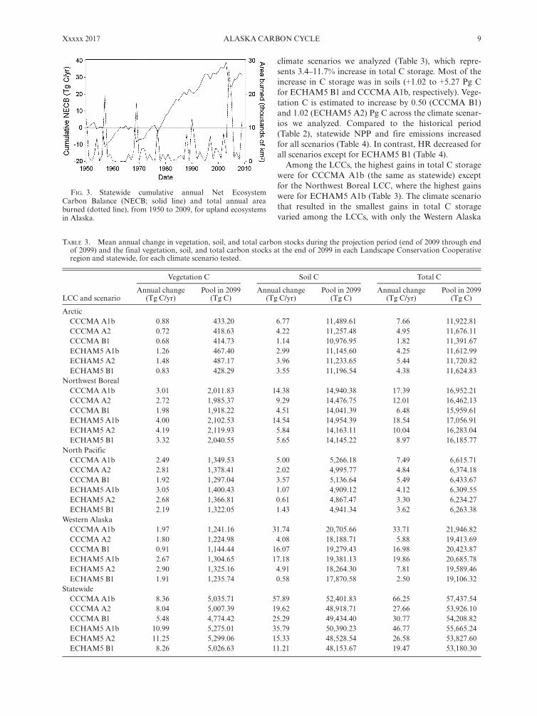
climate scenarios we analyzed (Table 3), which repre-sents 3.4–11.7% increase in total C storage. Most of theincrease in C storage was in soils (+1.02 to +5.27 Pg Cfor ECHAM5 B1 and CCCMA A1b, respectively). Vege-tation C is estimated to increase by 0.50 (CCCMA B1)and 1.02 (ECHAM5 A2) Pg C across the climate scenar-ios we analyzed. Compared to the historical period(Table 2), statewide NPP and fire emissions increasedfor all scenarios (Table 4). In contrast, HR decreased forall scenarios except for ECHAM5 B1 (Table 4).Among the LCCs, the highest gains in total C storage

were for CCCMA A1b (the same as statewide) exceptfor the Northwest Boreal LCC, where the highest gainswere for ECHAM5 A1b (Table 3). The climate scenariothat resulted in the smallest gains in total C storagevaried among the LCCs, with only the Western Alaska

FIG. 3. Statewide cumulative annual Net EcosystemCarbon Balance (NECB; solid line) and total annual areaburned (dotted line), from 1950 to 2009, for upland ecosystemsin Alaska.

TABLE 3. Mean annual change in vegetation, soil, and total carbon stocks during the projection period (end of 2009 through endof 2099) and the final vegetation, soil, and total carbon stocks at the end of 2099 in each Landscape Conservation Cooperativeregion and statewide, for each climate scenario tested.

Vegetation C Soil C Total C

LCC and scenarioAnnual change


(Tg C)Annual change


(Tg C)Annual change


(Tg C)

ArcticCCCMA A1b 0.88 433.20 6.77 11,489.61 7.66 11,922.81CCCMA A2 0.72 418.63 4.22 11,257.48 4.95 11,676.11CCCMA B1 0.68 414.73 1.14 10,976.95 1.82 11,391.67ECHAM5 A1b 1.26 467.40 2.99 11,145.60 4.25 11,612.99ECHAM5 A2 1.48 487.17 3.96 11,233.65 5.44 11,720.82ECHAM5 B1 0.83 428.29 3.55 11,196.54 4.38 11,624.83

Northwest BorealCCCMA A1b 3.01 2,011.83 14.38 14,940.38 17.39 16,952.21CCCMA A2 2.72 1,985.37 9.29 14,476.75 12.01 16,462.13CCCMA B1 1.98 1,918.22 4.51 14,041.39 6.48 15,959.61ECHAM5 A1b 4.00 2,102.53 14.54 14,954.39 18.54 17,056.91ECHAM5 A2 4.19 2,119.93 5.84 14,163.11 10.04 16,283.04ECHAM5 B1 3.32 2,040.55 5.65 14,145.22 8.97 16,185.77

North PacificCCCMA A1b 2.49 1,349.53 5.00 5,266.18 7.49 6,615.71CCCMA A2 2.81 1,378.41 2.02 4,995.77 4.84 6,374.18CCCMA B1 1.92 1,297.04 3.57 5,136.64 5.49 6,433.67ECHAM5 A1b 3.05 1,400.43 1.07 4,909.12 4.12 6,309.55ECHAM5 A2 2.68 1,366.81 0.61 4,867.47 3.30 6,234.27ECHAM5 B1 2.19 1,322.05 1.43 4,941.34 3.62 6,263.38

Western AlaskaCCCMA A1b 1.97 1,241.16 31.74 20,705.66 33.71 21,946.82CCCMA A2 1.80 1,224.98 4.08 18,188.71 5.88 19,413.69CCCMA B1 0.91 1,144.44 16.07 19,279.43 16.98 20,423.87ECHAM5 A1b 2.67 1,304.65 17.18 19,381.13 19.86 20,685.78ECHAM5 A2 2.90 1,325.16 4.91 18,264.30 7.81 19,589.46ECHAM5 B1 1.91 1,235.74 0.58 17,870.58 2.50 19,106.32

StatewideCCCMA A1b 8.36 5,035.71 57.89 52,401.83 66.25 57,437.54CCCMA A2 8.04 5,007.39 19.62 48,918.71 27.66 53,926.10CCCMA B1 5.48 4,774.42 25.29 49,434.40 30.77 54,208.82ECHAM5 A1b 10.99 5,275.01 35.79 50,390.23 46.77 55,665.24ECHAM5 A2 11.25 5,299.06 15.33 48,528.54 26.58 53,827.60ECHAM5 B1 8.26 5,026.63 11.21 48,153.67 19.47 53,180.30


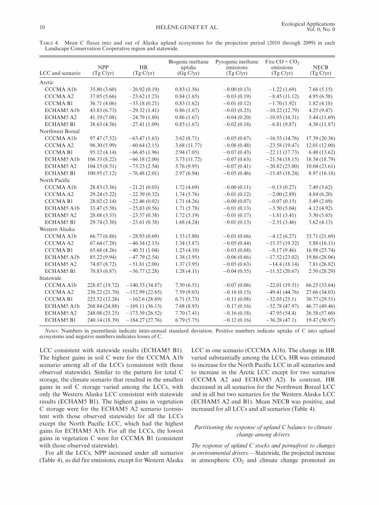
LCC consistent with statewide results (ECHAM5 B1).The highest gains in soil C were for the CCCMA A1bscenario among all of the LCCs (consistent with thoseobserved statewide). Similar to the pattern for total Cstorage, the climate scenario that resulted in the smallestgains in soil C storage varied among the LCCs, withonly the Western Alaska LCC consistent with statewideresults (ECHAM5 B1). The highest gains in vegetationC storage were for the ECHAM5 A2 scenario (consis-tent with those observed statewide) for all the LCCsexcept the North Pacific LCC, which had the highestgains for ECHAM5 A1b. For all the LCCs, the lowestgains in vegetation C were for CCCMA B1 (consistentwith those observed statewide).For all the LCCs, NPP increased under all scenarios

(Table 4), as did fire emissions, except for Western Alaska

LCC in one scenario (CCCMA A1b). The change in HRvaried substantially among the LCCs. HRwas estimatedto increase for the North Pacific LCC in all scenarios andto increase in the Arctic LCC except for two scenarios(CCCMA A2 and ECHAM5 A2). In contrast, HRdecreased in all scenarios for the Northwest Boreal LCCand in all but two scenarios for the Western Alaska LCC(ECHAM5 A2 and B1). Mean NECB was positive, andincreased for all LCCs and all scenarios (Table 4).

Partitioning the response of upland C balance to climatechange among drivers

The response of upland C stocks and permafrost to changesin environmental drivers.—Statewide, the projected increasein atmospheric CO2 and climate change promoted an

TABLE 4. Mean C fluxes into and out of Alaska upland ecosystems for the projection period (2010 through 2099) in eachLandscape Conservation Cooperative region and statewide.

LCC and scenarioNPP

(Tg C/yr)HR

(Tg C/yr)

Biogenic methaneuptake

(Gg C/yr)

Pyrogenic methaneemissions(Tg C/yr)

Fire CO + CO2emissions(Tg C/yr)

NECB(Tg C/yr)

ArcticCCCMA A1b 35.80 (3.60) �26.92 (0.19) 0.83 (1.56) �0.00 (0.13) �1.22 (1.69) 7.66 (5.15)CCCMA A2 37.05 (5.66) �23.62 (1.23) 0.84 (1.65) �0.03 (0.19) �8.45 (11.12) 4.95 (6.58)CCCMA B1 36.71 (4.06) �33.18 (0.21) 0.83 (1.62) �0.01 (0.12) �1.70 (1.92) 1.82 (4.18)ECHAM5 A1b 43.83 (6.73) �29.32 (1.41) 0.86 (1.67) �0.03 (0.25) �10.22 (12.79) 4.25 (9.47)ECHAM5 A2 41.19 (7.08) �24.79 (1.80) 0.86 (1.67) �0.04 (0.20) �10.93 (16.31) 5.44 (11.69)ECHAM5 B1 38.63 (4.56) �27.41 (1.09) 0.85 (1.67) �0.02 (0.18) �6.81 (9.87) 4.38 (11.87)

Northwest BorealCCCMA A1b 97.47 (7.52) �63.47 (1.63) 3.62 (8.71) �0.05 (0.67) �16.55 (14.76) 17.39 (20.36)CCCMA A2 96.30 (5.99) �60.64 (2.15) 3.68 (11.77) �0.08 (0.48) �23.58 (19.47) 12.01 (12.00)CCCMA B1 95.12 (4.14) �66.45 (1.96) 2.94 (7.05) �0.07 (0.43) �22.11 (17.73) 6.48 (13.62)ECHAM5 A1b 106.33 (8.22) �66.18 (2.00) 3.73 (11.72) �0.07 (0.63) �21.54 (18.15) 18.54 (18.79)ECHAM5 A2 104.15 (8.51) �73.23 (2.54) 3.76 (9.95) �0.07 (0.41) �20.82 (23.00) 10.04 (23.61)ECHAM5 B1 100.95 (7.12) �76.48 (2.01) 2.97 (6.94) �0.05 (0.46) �15.45 (18.24) 8.97 (16.18)

North PacificCCCMA A1b 28.83 (3.36) �21.21 (0.03) 1.72 (4.69) �0.00 (0.11) �0.13 (0.27) 7.49 (3.62)CCCMA A2 29.24 (5.22) �22.39 (0.32) 1.74 (5.76) �0.01 (0.12) �2.00 (2.89) 4.84 (6.20)CCCMA B1 28.02 (2.14) �22.46 (0.02) 1.71 (4.26) �0.00 (0.07) �0.07 (0.15) 5.49 (2.69)ECHAM5 A1b 33.47 (5.58) �25.83 (0.56) 1.71 (5.78) �0.01 (0.13) �3.50 (5.04) 4.12 (4.92)ECHAM5 A2 28.68 (3.55) �23.57 (0.38) 1.72 (5.19) �0.01 (0.17) �1.81 (3.41) 3.30 (5.65)ECHAM5 B1 29.74 (3.30) �23.61 (0.38) 1.68 (4.24) �0.01 (0.13) �2.51 (3.46) 3.62 (4.13)

Western AlaskaCCCMA A1b 66.77 (6.86) �28.93 (0.69) 1.33 (3.80) �0.01 (0.66) �4.12 (6.27) 33.71 (21.69)CCCMA A2 67.64 (7.28) �46.34 (2.13) 1.34 (3.87) �0.05 (0.44) �15.37 (19.32) 5.88 (16.11)CCCMA B1 65.68 (4.26) �40.51 (1.04) 1.23 (4.10) �0.03 (0.68) �8.17 (9.46) 16.98 (23.74)ECHAM5 A1b 85.22 (9.94) �47.79 (2.54) 1.38 (3.95) �0.06 (0.66) �17.52 (23.02) 19.86 (28.06)ECHAM5 A2 74.07 (8.72) �51.81 (2.00) 1.37 (3.95) �0.05 (0.63) �14.4 (18.14) 7.81 (26.82)ECHAM5 B1 70.83 (6.87) �56.77 (2.28) 1.28 (4.11) �0.04 (0.55) �11.52 (20.67) 2.50 (28.29)

StatewideCCCMA A1b 228.87 (19.72) �140.53 (34.87) 7.50 (6.51) �0.07 (0.06) �22.01 (19.51) 66.25 (33.64)CCCMA A2 230.22 (21.70) �152.99 (22.65) 7.59 (9.03) �0.16 (0.15) �49.41 (44.76) 27.66 (34.03)CCCMA B1 225.52 (12.26) �162.6 (28.69) 6.71 (5.73) �0.11 (0.08) �32.05 (25.1) 30.77 (29.51)ECHAM5 A1b 268.84 (24.88) �169.11 (36.13) 7.68 (8.95) �0.17 (0.16) �52.78 (47.97) 46.77 (49.46)ECHAM5 A2 248.08 (25.25) �173.39 (26.52) 7.70 (7.41) �0.16 (0.18) �47.95 (54.4) 26.58 (57.60)ECHAM5 B1 240.14 (18.39) �184.27 (27.76) 6.79 (5.75) �0.12 (0.16) �36.28 (47.1) 19.47 (50.97)

Notes: Numbers in parenthesis indicate inter-annual standard deviation. Positive numbers indicate uptake of C into uplandecosystems and negative numbers indicates losses of C.


Vol. 0, No. 0

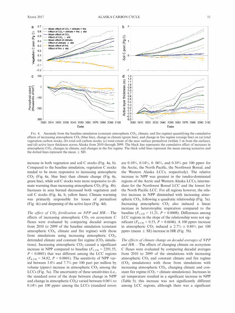
increase in both vegetation and soil C stocks (Fig. 4a, b).Compared to the baseline simulation, vegetation C stockstended to be more responsive to increasing atmosphericCO2 (Fig. 4a, blue line) than climate change (Fig. 4a,green line), while soil C stocks were more responsive to cli-mate warming than increasing atmospheric CO2 (Fig. 4b).Increases in area burned decreased both vegetation andsoil C stocks (Fig. 4a, b, yellow lines). Climate warmingwas primarily responsible for losses of permafrost(Fig. 4c) and deepening of the active layer (Fig. 4d).

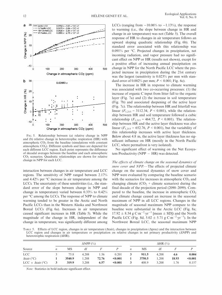
The effect of CO2 fertilization on NPP and HR.—Theeffects of increasing atmospheric CO2 on ecosystem Cfluxes were evaluated by comparing decadal averagesfrom 2010 to 2099 of the baseline simulation (constantatmospheric CO2, climate and fire regime) with thosefrom simulations using increasing atmospheric CO2,detrended climate and constant fire regime (CO2 simula-tions). Increasing atmospheric CO2 caused a significantincrease in NPP compared to baseline (F1,136 = 2291.55,P < 0.0001) that was different among the LCC regions(F4,136 = 34.82, P < 0.0001). The sensitivity of NPP var-ied between 3.8% and 7.7% per 100 part per million byvolume (ppmv) increase in atmospheric CO2 among theLCCs (Fig. 5a). The uncertainty of these sensitivities (i.e.,the standard error of the slope between change in NPPand change in atmospheric CO2) varied between 0.06% to0.14% per 100 ppmv among the LCCs (standard errors

are 0.10%, 0.14%, 0. 06%, and 0.10% per 100 ppmv forthe Arctic, the North Pacific, the Northwest Boreal, andthe Western Alaska LCCs, respectively). The relativeincrease in NPP was greatest in the tundra-dominatedregions of the Arctic and Western Alaska LCCs, interme-diate for the Northwest Boreal LCC and the lowest forthe North Pacific LCC. For all regions however, the rela-tive increase in NPP diminished with increasing atmo-spheric CO2, following a quadratic relationship (Fig. 5a).Increasing atmospheric CO2 also induced a linearincrease in heterotrophic respiration compared to thebaseline (F1,136 = 11.21, P = 0.0008). Differences amongLCC regions in the slope of the relationship were not sig-nificant (F4,136 = 0.53, P = 0.6646). A 100 ppmv increasein atmospheric CO2 induced a 2.7% � 0.86% per 100ppmv (mean � SE) increase in HR (Fig. 5b).

The effects of climate change on decadal averages of NPPand HR.—The effects of changing climate on ecosystemC fluxes were evaluated by comparing decadal averagesfrom 2010 to 2099 of the simulations with increasingatmospheric CO2 and constant climate and fire regime(CO2 simulations) with those from simulations withincreasing atmospheric CO2, changing climate and con-stant fire regime (CO2 + climate simulations). Increases inair temperature resulted in a significant increase in NPP(Table 5); this increase was not significantly differentamong LCC regions, although there was a significant

FIG. 4. Anomaly from the baseline simulation (constant atmospheric CO2, climate, and fire regime) quantifying the cumulativeeffects of increasing atmospheric CO2 (blue line), change in climate (green line), and change in fire regime (orange line) on (a) totalvegetation carbon stocks, (b) total soil carbon stocks, (c) total extent of the near surface permafrost (within 3 m from the surface),and (d) active layer thickness across Alaska from 2010 through 2099. The black line represents the cumulative effect of increases inatmospheric CO2, changes in climate, and changes in the fire regime. The thick solid lines represent the mean among scenarios andthe dotted lines represent the mean � SD.


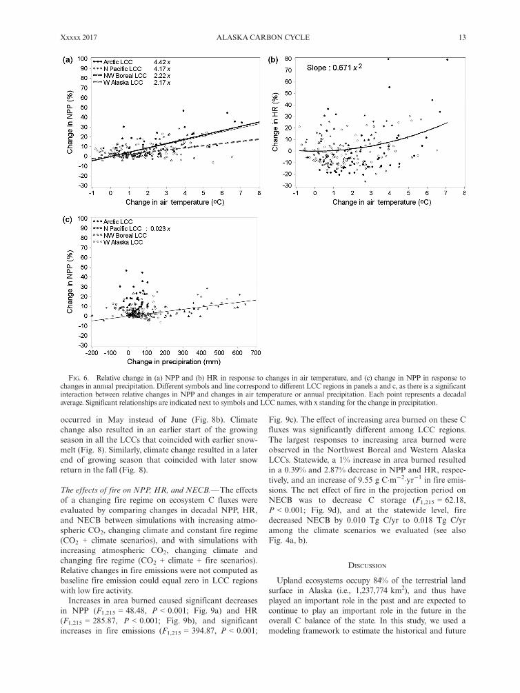
interaction between changes in air temperature and LCCregions. The sensitivity of NPP ranged between 2.17%and 4.42% per °C increase in air temperature among theLCCs. The uncertainty of these sensitivities (i.e., the stan-dard error of the slope between change in NPP andchange in temperature) varied between 0.33% to 0.42%per °C among the LCCs. The response of NPP to climatewarming tended to be greater in the Arctic and NorthPacific LCCs than in the Western Alaska and NorthwestBoreal LCCs (Fig. 6a). Increases in air temperaturecaused significant increases in HR (Table 5). While themagnitude of the change in HR, independent of thechange in temperature, was significantly different among

LCCs (ranging from �10.06% to �1.13%), the responseto warming (i.e., the slope between change in HR andchange in air temperature) was not (Table 5). The overallresponse of HR to changes in air temperature follows anupward sloping quadratic relationship (Fig. 6b). Thestandard error associated with this relationship was0.091% per °C. Projected changes in precipitation, netincoming radiation, and vapor pressure had no signifi-cant effect on NPP or HR (results not shown), except fora positive effect of increasing annual precipitation onchange in NPP for the North Pacific LCC where the pro-jected increase in precipitation during the 21st centurywas the largest (sensitivity is 0.023% per mm with stan-dard error of 0.002% per mm; P < 0.001; Fig. 6c).The increase in HR in response to climate warming

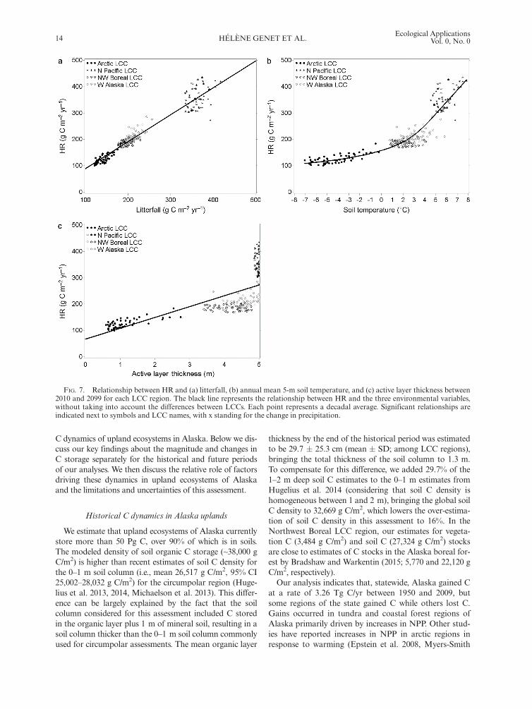
was associated with two co-occurring processes: (1) theincrease of organic C input from litter fall to the organiclayer (Fig. 7a) and (2) the increase in soil temperature(Fig. 7b) and associated deepening of the active layer(Fig. 7c). The relationship between HR and litterfall waslinear (F1,215 = 3112.34, P < 0.001), while the relation-ship between HR and soil temperature followed a cubicrelationship (F1,215 = 464.72, P < 0.001). The relation-ship between HR and the active layer thickness was alsolinear (F1,215 = 652.76, P < 0.001), but the variability ofthis relationship increases with active layer thickness.Below about 4.8 m, the active layer thickness has no sig-nificant influence on HR (mostly in the North PacificLCC, where permafrost is very isolated).No significant effect of warming on the Net Ecosys-

tem Productivity (NPP � HR) was detected.

The effects of climate change on the seasonal dynamics ofsnow cover and NPP.—The effects of projected climatechange on the seasonal dynamics of snow cover andNPP were evaluated by comparing the baseline scenariowith the scenarios for increases in atmospheric CO2 andchanging climate (CO2 + climate scenarios) during thefinal decade of the projection period (2090–2099). Com-pared to the baseline, the increase in atmospheric CO2

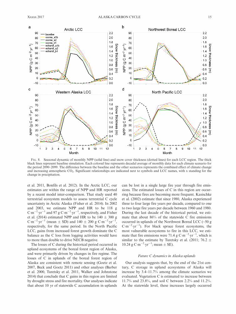
and climate change caused an increase in the seasonalmaximum of NPP in all LCC regions. Changes in themagnitude of seasonal maximum NPP compare to thebaseline were substantial in the Arctic LCC (Fig. 8a;17.92 � 8.54 g C�m�2�yr�1 [mean � SD]) and the NorthPacific LCC (Fig. 8d, 5.02 � 5.71 g C�m�2�yr�1). In theNorthwest Boreal LCC, the seasonal maximum NPP

FIG. 5. Relationship between (a) relative change in NPPand (b) relative change in heterotrophic respiration (HR) withatmospheric CO2 from the baseline (simulations with constantatmospheric CO2). Different symbols and lines are depicted foreach different LCC region. Each point represents the differenceof decadal averages between the baseline and each atmosphericCO2 scenarios. Quadratic relationships are shown for relativechange in NPP for each LCC.

TABLE 5. Effects of LCC region, changes in air temperature (Dtair), changes in precipitation (Dprec) and the interaction betweenLCC region and changes in air temperature or precipitation on relative changes in net primary productivity (DNPP) andheterotrophic respiration (DHR).

Source

DNPP (%) DHR (%)

n MS df F P n MS df F P

LCC 3 75.8 4,208 1.56 0.201 3 911.5 4,208 4.6 0.004Dtair (°C) 1 3540.9 1,208 72.76 <0.001 1 3750.5 1,208 18.93 <0.001LCC 9 Dtair (°C) 3 319.9 3,208 6.57 <0.001 3 408.9 3,208 1.76 0.157

Note: Statistics in bold indicate significant effect.


Vol. 0, No. 0

occurred in May instead of June (Fig. 8b). Climatechange also resulted in an earlier start of the growingseason in all the LCCs that coincided with earlier snow-melt (Fig. 8). Similarly, climate change resulted in a laterend of growing season that coincided with later snowreturn in the fall (Fig. 8).

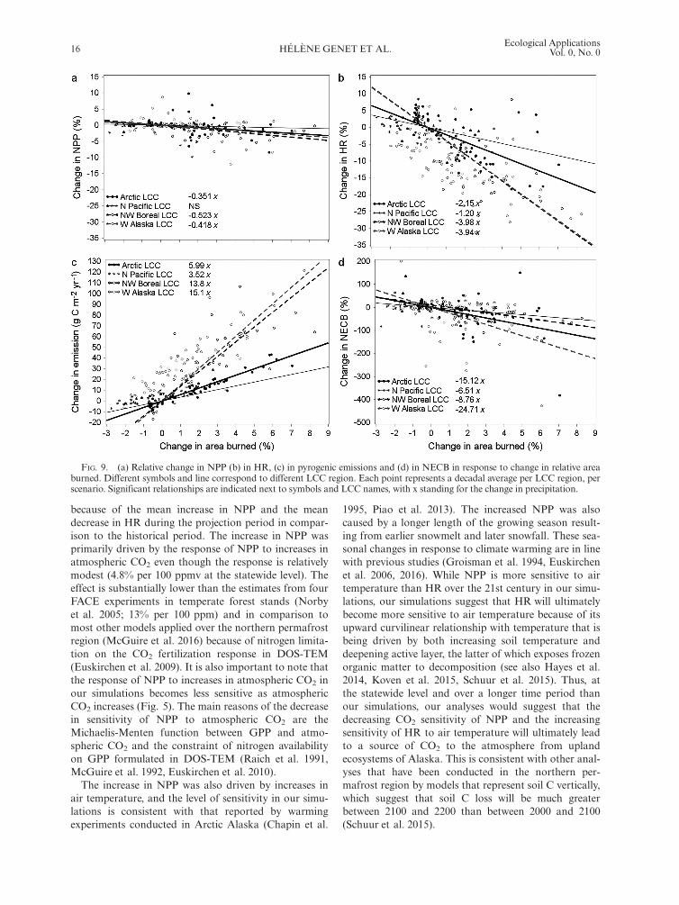
The effects of fire on NPP, HR, and NECB.—The effectsof a changing fire regime on ecosystem C fluxes wereevaluated by comparing changes in decadal NPP, HR,and NECB between simulations with increasing atmo-spheric CO2, changing climate and constant fire regime(CO2 + climate scenarios), and with simulations withincreasing atmospheric CO2, changing climate andchanging fire regime (CO2 + climate + fire scenarios).Relative changes in fire emissions were not computed asbaseline fire emission could equal zero in LCC regionswith low fire activity.Increases in area burned caused significant decreases

in NPP (F1,215 = 48.48, P < 0.001; Fig. 9a) and HR(F1,215 = 285.87, P < 0.001; Fig. 9b), and significantincreases in fire emissions (F1,215 = 394.87, P < 0.001;

Fig. 9c). The effect of increasing area burned on these Cfluxes was significantly different among LCC regions.The largest responses to increasing area burned wereobserved in the Northwest Boreal and Western AlaskaLCCs. Statewide, a 1% increase in area burned resultedin a 0.39% and 2.87% decrease in NPP and HR, respec-tively, and an increase of 9.55 g C�m�2�yr�1 in fire emis-sions. The net effect of fire in the projection period onNECB was to decrease C storage (F1,215 = 62.18,P < 0.001; Fig. 9d), and at the statewide level, firedecreased NECB by 0.010 Tg C/yr to 0.018 Tg C/yramong the climate scenarios we evaluated (see alsoFig. 4a, b).

DISCUSSION

Upland ecosystems occupy 84% of the terrestrial landsurface in Alaska (i.e., 1,237,774 km2), and thus haveplayed an important role in the past and are expected tocontinue to play an important role in the future in theoverall C balance of the state. In this study, we used amodeling framework to estimate the historical and future

FIG. 6. Relative change in (a) NPP and (b) HR in response to changes in air temperature, and (c) change in NPP in response tochanges in annual precipitation. Different symbols and line correspond to different LCC regions in panels a and c, as there is a significantinteraction between relative changes in NPP and changes in air temperature or annual precipitation. Each point represents a decadalaverage. Significant relationships are indicated next to symbols and LCC names, with x standing for the change in precipitation.


C dynamics of upland ecosystems in Alaska. Below we dis-cuss our key findings about the magnitude and changes inC storage separately for the historical and future periodsof our analyses. We then discuss the relative role of factorsdriving these dynamics in upland ecosystems of Alaskaand the limitations and uncertainties of this assessment.

Historical C dynamics in Alaska uplands

We estimate that upland ecosystems of Alaska currentlystore more than 50 Pg C, over 90% of which is in soils.The modeled density of soil organic C storage (~38,000 gC/m2) is higher than recent estimates of soil C density forthe 0–1 m soil column (i.e., mean 26,517 g C/m2, 95% CI25,002–28,032 g C/m2) for the circumpolar region (Huge-lius et al. 2013, 2014, Michaelson et al. 2013). This differ-ence can be largely explained by the fact that the soilcolumn considered for this assessment included C storedin the organic layer plus 1 m of mineral soil, resulting in asoil column thicker than the 0–1 m soil column commonlyused for circumpolar assessments. The mean organic layer

thickness by the end of the historical period was estimatedto be 29.7 � 25.3 cm (mean � SD; among LCC regions),bringing the total thickness of the soil column to 1.3 m.To compensate for this difference, we added 29.7% of the1–2 m deep soil C estimates to the 0–1 m estimates fromHugelius et al. 2014 (considering that soil C density ishomogeneous between 1 and 2 m), bringing the global soilC density to 32,669 g C/m2, which lowers the over-estima-tion of soil C density in this assessment to 16%. In theNorthwest Boreal LCC region, our estimates for vegeta-tion C (3,484 g C/m2) and soil C (27,324 g C/m2) stocksare close to estimates of C stocks in the Alaska boreal for-est by Bradshaw and Warkentin (2015; 5,770 and 22,120 gC/m2, respectively).Our analysis indicates that, statewide, Alaska gained C

at a rate of 3.26 Tg C/yr between 1950 and 2009, butsome regions of the state gained C while others lost C.Gains occurred in tundra and coastal forest regions ofAlaska primarily driven by increases in NPP. Other stud-ies have reported increases in NPP in arctic regions inresponse to warming (Epstein et al. 2008, Myers-Smith

FIG. 7. Relationship between HR and (a) litterfall, (b) annual mean 5-m soil temperature, and (c) active layer thickness between2010 and 2099 for each LCC region. The black line represents the relationship between HR and the three environmental variables,without taking into account the differences between LCCs. Each point represents a decadal average. Significant relationships areindicated next to symbols and LCC names, with x standing for the change in precipitation.


Vol. 0, No. 0

et al. 2011, Bonfils et al. 2012). In the Arctic LCC, ourestimates are within the range of NPP and HR reportedby a recent model inter-comparison. That study used 40terrestrial ecosystem models to assess terrestrial C cycleuncertainty in Arctic Alaska (Fisher et al. 2014). In 2002and 2003, we estimate NPP and HR to be 118 gC�m�2�yr�1 and 97 g C�m�2�yr�1, respectively, and Fisheret al. (2014) estimated NPP and HR to be 140 � 300 gC�m�2�yr�1 (mean � SD) and 140 � 200 g C�m�2�yr�1,respectively, for the same period. In the North PacificLCC, gains from increased forest growth dominate the Cbalance as the C loss from logging activities would haveto more than double to drive NECB negative.The losses of C during the historical period occurred in

upland ecosystems of the boreal forest region of Alaska,and were primarily driven by changes in fire regime. Thelosses of C in uplands of the boreal forest region ofAlaska are consistent with remote sensing (Goetz et al.2007, Beck and Goetz 2011) and other analyses (Barberet al. 2000, Turetsky et al. 2011, Walker and Johnstone2014) that conclude that C gains in this region are limitedby drought stress and fire mortality. Our analyses indicatethat about 10 yr of statewide C accumulation in uplands

can be lost in a single large fire year through fire emis-sions. The estimated losses of C in this region are occur-ring because fires are becoming more frequent. Kasischkeet al. (2002) estimate that since 1980, Alaska experiencedthree to four large fire years per decade, compared to oneto two large fire years per decade between 1960 and 1980.During the last decade of the historical period, we esti-mate that about 86% of the statewide C fire emissionsoccurred in uplands of the Northwest Boreal LCC (~50 gC�m�2�yr�1). For black spruce forest ecosystems, themost vulnerable ecosystems to fire in this LCC, we esti-mate that fire emissions were 71.4 g C�m�2�yr�1, which issimilar to the estimate by Turetsky et al. (2011; 76.2 �10.24 g C�m�2�yr�1; mean � SE).

Future C dynamics in Alaska uplands

Our analysis suggests that, by the end of the 21st cen-tury, C storage in upland ecosystems of Alaska willincrease by 3.4–11.7% among the climate scenarios weevaluated. Vegetation C is estimated to increase between11.7% and 23.8%, and soil C between 2.2% and 11.2%.At the statewide level, these increases largely occurred

FIG. 8. Seasonal dynamic of monthly NPP (solid line) and snow cover thickness (dotted lines) for each LCC region. The thickblack lines represent baseline simulation. Each colored line represents decadal average of monthly data for each climate scenario forthe period 2090–2099. The difference between the baseline and the other scenarios represents the combined effect of climate changeand increasing atmospheric CO2. Significant relationships are indicated next to symbols and LCC names, with x standing for thechange in precipitation.


because of the mean increase in NPP and the meandecrease in HR during the projection period in compar-ison to the historical period. The increase in NPP wasprimarily driven by the response of NPP to increases inatmospheric CO2 even though the response is relativelymodest (4.8% per 100 ppmv at the statewide level). Theeffect is substantially lower than the estimates from fourFACE experiments in temperate forest stands (Norbyet al. 2005; 13% per 100 ppm) and in comparison tomost other models applied over the northern permafrostregion (McGuire et al. 2016) because of nitrogen limita-tion on the CO2 fertilization response in DOS-TEM(Euskirchen et al. 2009). It is also important to note thatthe response of NPP to increases in atmospheric CO2 inour simulations becomes less sensitive as atmosphericCO2 increases (Fig. 5). The main reasons of the decreasein sensitivity of NPP to atmospheric CO2 are theMichaelis-Menten function between GPP and atmo-spheric CO2 and the constraint of nitrogen availabilityon GPP formulated in DOS-TEM (Raich et al. 1991,McGuire et al. 1992, Euskirchen et al. 2010).The increase in NPP was also driven by increases in

air temperature, and the level of sensitivity in our simu-lations is consistent with that reported by warmingexperiments conducted in Arctic Alaska (Chapin et al.

1995, Piao et al. 2013). The increased NPP was alsocaused by a longer length of the growing season result-ing from earlier snowmelt and later snowfall. These sea-sonal changes in response to climate warming are in linewith previous studies (Groisman et al. 1994, Euskirchenet al. 2006, 2016). While NPP is more sensitive to airtemperature than HR over the 21st century in our simu-lations, our simulations suggest that HR will ultimatelybecome more sensitive to air temperature because of itsupward curvilinear relationship with temperature that isbeing driven by both increasing soil temperature anddeepening active layer, the latter of which exposes frozenorganic matter to decomposition (see also Hayes et al.2014, Koven et al. 2015, Schuur et al. 2015). Thus, atthe statewide level and over a longer time period thanour simulations, our analyses would suggest that thedecreasing CO2 sensitivity of NPP and the increasingsensitivity of HR to air temperature will ultimately leadto a source of CO2 to the atmosphere from uplandecosystems of Alaska. This is consistent with other anal-yses that have been conducted in the northern per-mafrost region by models that represent soil C vertically,which suggest that soil C loss will be much greaterbetween 2100 and 2200 than between 2000 and 2100(Schuur et al. 2015).

FIG. 9. (a) Relative change in NPP (b) in HR, (c) in pyrogenic emissions and (d) in NECB in response to change in relative areaburned. Different symbols and line correspond to different LCC region. Each point represents a decadal average per LCC region, perscenario. Significant relationships are indicated next to symbols and LCC names, with x standing for the change in precipitation.


Vol. 0, No. 0

Fire is an important disturbance that has a complicatedeffect on the projected increases in C storage in our simu-lations. Mean annual area burned in the projection periodranged from �81.5% to +169.3% of that during the histor-ical period. Our analysis shows that increased area burnedtends to decrease NPP, decrease HR, and increase fireemissions. The decrease in NPP is associated with treemortality and the decrease in HR following wildfire isrelated to the partial or total burning of the organic hori-zons during combustion and the decrease in C input fromvegetation litterfall. In fire-prone regions, our study sug-gests that decreases in HR from wildfire can be greaterthan increases resulting from warming (and increasingvegetation productivity) associated with increasing CO2

and climate change in those regions. As a result, HRdecreases during the projection period in the two largestand most fire-prone LCC regions, namely the NorthwestBoreal and the Western AK LCCs, where on average56.2% � 13.5% and 23.2% � 11.4% (mean � SD amongclimate scenarios) of the area burns every 100 yr, respec-tively (Rupp et al. 2016). Statewide, the decrease in HRfrom these two LCCs is greater than the increase in HRprojected in the less fire-prone Arctic and the North Paci-fic LCCs, resulting in an overall decrease of 9.1% in HR(8.6% SD among climate scenarios) in comparison to thehistorical period. The net result is that increases in firedecrease NECB and cause losses in both vegetation andsoil C. Whether fire will continue to limit gains (or pro-mote losses) of C from upland ecosystems of Alaskadepends on feedbacks between vegetation compositionand the occurrence of fire. The increase in fire severity andfire frequency can promote the establishment of deciduousforest (e.g., Johnstone et al. 2010b, Pastick et al. 2017).Because deciduous forest is less flammable than blackspruce forest (Bernier et al. 2016), the transition fromevergreen to deciduous vegetation could result in less fireon the landscape in the latter part of this century. Thisinteraction between vegetation composition and fireregime is represented in this study since ALFRESCO rep-resents the effect of fire severity on post-fire vegetationsuccession and the feedback of vegetation composition onfire regime (see Pastick et al. this feature). However, sincethe vegetation composition in DOS-TEM is consideredstatic, the direct effect of changes in vegetation composi-tion on carbon dynamics was not included.Across the projection period, NECB was larger in tun-

dra-dominated regions (the Arctic and Western AlaskaLCCs) and the North Pacific LCC than in the North-west Boreal LCC. The increase in fire was the primaryreason for the more muted response of the NorthwestBoreal LCC in comparison to the other LCCs, where theresponses of NPP to increases in atmospheric CO2 andincreased temperature primarily drove the larger NECB.Regions of largest uncertainties among the climate sce-narios, for example the Yukon-Kuskokwim Delta or thenorthern Seward Peninsula, were also regions that expe-rienced the largest increase in length of the growing sea-son, as shown in Fig. S2 of Pastick et al. (this feature).

In past syntheses of regional C dynamics, the role ofaerated soils as a sink for CH4 has generally beenneglected. Consistent with field observations (Whalenand Reeburgh 1990, Moosavi and Crill 1997, Martineauet al. 2010), this assessment shows that biogenic CH4

fluxes in upland Alaska were a net sink from the atmo-sphere. Other analyses suggest that biogenic CH4 seques-tration in upland soils should increase during the 21stcentury (Zhuang et al. 2013) in response to an increase inlitter organic C input and soil temperature (Walter andHeimann 2000, Hofmann et al. 2016) and an increase inunsaturated soil volume resulting from permafrost thawand deepening the water table (Whalen and Reeburgh1990, Zhuang et al. 2004). However, our analysis suggeststhat the effects of climate change on biogenic CH4 seques-tration would be trivial at the regional scale, and thatCH4 balance in uplands would primarily be driven bypyrogenic emissions of CH4. The pyrogenic CH4 lossfrom uplands ecosystems is relatively minor, as it repre-sents less than 0.1% of upland NPP.

Limitation and uncertainties of projections of C balance inupland Alaska

This assessment of C dynamics in upland ecosystemsof Alaska provided estimates of the uncertainty associ-ated with forcing data, i.e., atmospheric CO2 for threeemission scenarios and climate projections from two glo-bal circulation models, on the regional C balance. State-wide, although the variability of NECB among the sixclimate scenarios was substantial (SD = 17.2 Tg C/yr), allscenarios predicted uplands to be a C sink by the end ofthe 21st century. The uncertainty of NECB associatedwith CO2 emission scenarios (SD = 17.6 Tg C/yr) was lar-ger than the uncertainty associated with GCMs (SD = 7.5Tg C/yr). As mentioned previously, the effect of forestlogging in the North Pacific LCC was not included in thefuture projections as explicit projections were not avail-able at the time this assessment was conducted. Yet, fromthe historical estimates, the total export of C from loggingactivities were quite small (i.e., 1.6 Tg C/yr). If projectedto be constant over the 21st century, these exports wouldhave had a minor effect on the estimated statewide C sink(i.e., 5.2% decrease of NECB on average, SD = 2.1%among climate scenarios). Furthermore, a recent attribu-tion analysis quantifying the relative effect of logging andclimate change on forest C stocks in the North PacificLCC suggested that the effect of harvesting on forest Cstocks for the 21st century was more than 27 timessmaller than the effect of climate change only (for theCCCMA-A1b scenario; Zhou et al. 2016).In addition to forcing data, model structure and pro-

cess representations can be a significant source of uncer-tainty in ecosystem carbon projections. A recent modelcomparison of the historical carbon balance in Alaska,compared model inter-comparison projects using similaror different forcing data and estimated that uncertaintyresulting from differences in model structure and process


representations can be larger than uncertainty resultingfrom differences in forcing data (Fisher et al. 2014).DOS-TEM explicitly represents processes that have beenidentified as critical to represent in high latitude ecosys-tems (McGuire et al. 2012, 2016, Koven et al. 2015, Luoet al. 2016). These processes include (1) soil thermalregime and permafrost dynamics and their effects on soilC dynamics (Yi et al. 2009b), (2) nitrogen limitation onvegetation productivity (Euskirchen et al. 2010), and (3)and organic layer dynamics on soil environmental andbiogeochemical processes (Yi et al. 2009a, 2010). How-ever, additional processes not represented in the model-ing framework used in this study can affect ecosystemdynamics at the regional level, and may change inresponse to climate change.The biogeochemical models used in this assessment did

not include a dynamic vegetation model, i.e., vegetationdistribution was static after initialization. Yet, with cli-mate change and change in disturbance regime, changesin vegetation composition are ongoing (e.g., Sturm et al.2001, Tape et al. 2006) and expected to continue over thecoming decades in the boreal and the Arctic regions (e.g.,Pastick et al. 2017), with the potential to cause significantchanges in the regional carbon balance. In the arcticregion, climate-related shrubification in the Arctic(Myers-Smith et al. 2011) is projected to offset the loss ofshrub tundra from increasing fire frequency (Pasticket al. 2017), and result in a decrease in soil temperaturethat can slow down decomposition of soil organic matterand reduce heterotrophic respiration (Sistla et al. 2013).The transition from graminoid to shrub tundra can alsocause an increase in vegetation productivity and vegeta-tion biomass (Shaver and Chapin 1991). In boreal forest,the projected increase in wildfire frequency and severitycan result in large-scale transition from spruce-dominatedforest to deciduous-dominated forest (e.g., Johnstoneet al. 2010b), which can lead to an increase in vegetationproductivity and litter quality and an increase in soil tem-perature and decomposition rates (Melvin et al. 2015).The current assessment is considering soil biogeochemi-

cal processes occurring in the organic layer and the firstmeter of the mineral soil. Yet, substantial amount oforganic C can be stored below this depth (Harden et al.2012a) and, with active layer deepening, can becomeunfrozen and be exposed to decomposition (Schuur et al.2009). Additionally, lateral loss of dissolved organic C(DOC) from terrestrial to aquatic ecosystems are not takeninto account in the modeling framework (Stackepooleet al. 2017). Yet, previous model simulations estimatedthat DOC loss can have a substantial effect on the regionalC balance, reducing the strength of the C sink in the Arcticregion (McGuire et al. 2010, Kicklighter et al. 2013).Finally, the degradation of permafrost in uplands may trig-ger thermal-erosion processes and the formation of fea-tures such as active layer detachments or retrogressivethaw slumps (Balser et al. 2014) with dramatic changes onlocal hydrology and vegetation that could affect substan-tially ecosystem C balance (Jensen et al. 2014).

Finally, studies quantifying the actual proportionbetween the quantity of wood harvested (and exportedout of the ecosystem) and the residues left on site inNorthern Pacific forests are very scarce. Given that clearcutting is the most common harvest practice in theregion (Cole et al. 2010), we used the highest proportionof cutting intensity estimated by Deal and Tappeiner(2002) to estimate C exported out of the ecosystem fromtimber harvest. Yet, our study might have underesti-mated the proportion of wood left on site after cutting.An older study by Howard and Setzer (1989) estimatesthat only 43.3–51.3% of the forest volume is exportedout of the ecosystem. A mean harvest rate of 47.3%would decrease the total C exported as timber from 1.6Tg C/yr to 0.80 Tg C/yr and would increase the histori-cal C sink from 3.26 Tg C/yr to 4.06 Tg C/yr.

CONCLUSION

This assessment of C dynamics in upland ecosystemsof Alaska is unique in that it explicitly separates uplandsfrom wetlands C dynamics. As in any assessment, thereare limitations and uncertainties. Key limitationsinclude (1) the treatment of land cover as static in theprojection period, and (2) the lack of consideration ofdisturbances in addition to fire such as those caused byinsects and thawing of ice-rich permafrost and associ-ated soil subsidence. It is well known that increased firedisturbance has the potential to increase the cover ofdeciduous forest at the expense of spruce forest (John-stone et al. 2010a,b). It is also expected that shrub tun-dra will expand at the expense of graminoid tundra(Myers-Smith et al. 2011). Insects and disease also sub-stantially affect forest productivity in the Alaska borealforest (Verbyla 2011), and there is evidence that insectdisturbance is increasing in Alaska (Parent and Verbyla2010). Finally, degradation of ice-rich permafrost inuplands has the potential to alter C cycling in the north-ern permafrost region (Grosse et al. 2011, Olefeldt et al.2016). Model modifications to deal with these issues arecurrently being developed so that these issues can bebetter addressed in future assessments. Despite theselimitations, our study provides important insights onregional vulnerability of C storage in Alaska. In particu-lar, our study indicates that projected C sequestration inthe Northwest Boreal LCC would be weakest amongthe LCCs. This suggests that this region would be mostvulnerable to becoming a C source during the remainderof the 21st century in response to other disturbancesand harvesting that we did not consider. Finally, even ifupland ecosystems as a whole are able to sequester Cthroughout the 21st century, our analysis indicates thatany increased C sequestration in upland ecosystems ofAlaska during the 21st century is likely to be transi-tional as NPP becomes less sensitive to increases inatmospheric CO2 and HR increases due to increase in Cinput from the vegetation, warmer soil, and a deeperactive layer.


Vol. 0, No. 0

ACKNOWLEDGMENTS

This research was funded by the U.S. Geological Survey(USGS) Land Change Science Program. Additional supportwas provided by (1) the Alaska Climate Science Center throughGrant/Cooperative Agreement G10AC00588 from the U.S.Geological Survey and (2) the National Science Foundationand the USDA Forest Service through the Bonanza Creek LongTerm Ecological Research Program. Any use of trade, firm, orproduct names is for descriptive purposes only and does notimply endorsement by the U.S. Government.

LITERATURE CITED

Abbott, B. W., et al. 2016. Biomass offsets little or none of per-mafrost carbon release from soils, streams, and wildfire: anexpert assessment. Environmental Research Letters 11:034014.

Ainsworth, E. A., and S. P. Long. 2005. What have we learnedfrom 15 years of free-air CO2 enrichment (FACE)? A meta-analytic review of the responses of photosynthesis, canopyproperties and plant production to rising CO2. New Phytolo-gist 165:351–372.

Alaback, P. B. 1982. Dynamics of understory biomass in Sitkaspruce-western hemlock forests of southeast Alaska. Ecology63:1932–1948.

Balser, A. W., J. B. Jones, and R. Gens. 2014. Timing of retro-gressive thaw slump initiation in the Noatak Basin, northwestAlaska, USA. Journal of Geophysical Research—Earth Sur-face 119:1106–1120.

Balshi, M. S., et al. 2007. The role of historical fire disturbancein the carbon dynamics of the pan-boreal region: A process-based analysis. Journal of Geophysical Research—Biogeo-sciences 112:2156–2202.

Balshi, M. S., A. D. McGuirez, P. Duffy, M. Flannigan,J. Walsh, and J. Melillo. 2009. Assessing the response of areaburned to changing climate in western boreal North Americausing a multivariate adaptive regression splines (MARS)approach. Global Change Biology 15:578–600.

Barber, V. A., G. P. Juday, and B. P. Finney. 2000. Reducedgrowth of Alaskan white spruce in the twentieth century fromtemperature-induced drought stress. Nature 405:668–673.

Beck, P. S. A., and S. J. Goetz. 2011. Satellite observations ofhigh northern latitude vegetation productivity changesbetween 1982 and 2008: ecological variability and regionaldifferences. Environmental Research Letters 6:045501.

Bekryaev, R. V., I. V. Polyakov, and V. A. Alexeev. 2010. Role ofpolar amplification in long-term surface air temperature vari-ations and modern arctic warming. Journal of Climate23:3888–3906.

Bernier, P. Y., S. Gauthier, P.-O. Jean, F. Manka, Y. Boulanger,A. Beaudoin, and L. Guindon. 2016. Mapping local effects offorest properties on fire risk across Canada. Forests 7:157.https://doi.org/10.3390/f7080157

Bhatti, J. S., M. J. Apps, and H. Jiang. 2010. Influence of nutri-ents, disturbances and site conditions on carbon stocks alonga boreal forest transect in central Canada. Plant and Soil242:1–14.

Bieniek, P. A., et al. 2015. Climate drivers linked to changingseasonality of Alaska coastal tundra vegetation productivity.Earth Interactions 19:19.

Binkley, D. 1982. Nitrogen-fixation and net primary productionin a young Sitka alder stand. Canadian Journal of Botany60:281–284.

Bonfils, C. J. W., T. J. Phillips, D. M. Lawrence, P. Cameron-Smith, W. J. Riley, and Z. M. Subin. 2012. On the influenceof shrub height and expansion on northern high latitudeclimate. Environmental Research Letters 7:015503.

Bradshaw, C. J. A., and I. G. Warkentin. 2015. Global estimatesof boreal forest carbon stocks and flux. Global and PlanetaryChange 128:24–30.

Brown, J. H., O. J. Ferrians Jr., J. A. Heginbottom, and E. S.Melnikov. 1998. Circum-arctic map of permafrost andground ice conditions. National Snow and Ice Data Center,Digital Media, Boulder, Colorado, USA.

CAVM Team. 2003. Circumpolar arctic vegetation map.(1:7,500,000 scale), Conservation of Arctic Flora and Fauna(CAFF) Map No. 1. U.S. Fish and Wildlife Service, Anchor-age, Alaska, USA.

Chapin III, F. S., G. R. Shaver, A. E. Giblin, K. J. Nadelhoffer,and J. A. Laundre. 1995. Responses of arctic tundra to experi-mental and observed changes in climate. Ecology 76:694–711.

Chapin III, F. S., M. D. Robards, H. P. Huntington, J. E. John-stone, S. E. Trainor, G. P. Kofinas, R. W. Ruess, N. Fresco,D. C. Natcher, and R. L. Naylor. 2006. Directional changesin ecological communities and social-ecological systems: Aframework for prediction based on Alaskan examples. Ameri-can Naturalist 168:S36–S49.

Clein, J. S., A. D. McGuire, X. Zhang, D. W. Kicklighter, J. M.Melillo, S. C. Wofsy, P. G. Jarvis, and J. M. Massheder. 2002.Historical and projected carbon balance of mature blackspruce ecosystems across North America: the role of carbon-nitrogen interactions. Plant and Soil 242:15–32.

Cole, E. C., T. A. Hanley, and M. Newton. 2010. Influence ofprecommercial thinning on understory vegetation of young-growth Sitka spruce forests in southeastern Alaska. CanadianJournal of Forest Research 40:619–628.

D’Amore, D. V., J. D. Fellman, R. T. Edwards, E. Hood, andC. L. Ping. 2012. Hydropedology of the North Americancoastal temperate rainforest. Pages 351–380 in H. Lin,editor. Hydropedology; synergystic integration of soil scienceand hydrology. Academic Press, Waltham, Massachusetts,USA.

De Groot, W. J., M. D. Flannigan, and A. S. Cantin. 2013.Climate change impacts on future boreal fire regimes. ForestEcology and Management 294:35–44.

Deal, R. L., and J. C. Tappeiner. 2002. The effects of partial cut-ting on stand structure and growth of western hemlock–Sitkaspruce stands in southeast Alaska. Forest Ecology and Man-agement 159:173–186.

Epstein, H. E., D. A. Walker, M. K. Raynolds, G. J. Jia, andA. M. Kelley. 2008. Phytomass patterns across a temperaturegradient of the North American arctic tundra. Journal ofGeophysical Research—Biogeosciences 113:2156–2202.

Euskirchen, E. S., et al. 2006. Importance of recent shifts in soilthermal dynamics on growing season length, productivity,and carbon sequestration in terrestrial high-latitude ecosys-tems. Global Change Biology 12:731–750.

Euskirchen, E. S., A. D. McGuire, and F. S. Chapin III. 2007.Energy feedbacks of northern high-latitude ecosystems to theclimate system due to reduced snow cover during 20thcentury warming. Global Change Biology 13:2425–2438.

Euskirchen, E. S., A. D. McGuire, F. S. Chapin III, and T. S.Rupp. 2010. The changing effects of Alaska’s boreal forestson the climate system. Canadian Journal of Forest Research40:1336–1346.

Euskirchen, E. S., A. D. McGuire, F. S. Chapin III, S. Yi, andC. C. Thompson. 2009. Changes in vegetation in northernAlaska under scenarios of climate change, 2003–2100: impli-cations for climate feedbacks. Ecological Applications 19:1022–1043.

Euskirchen, E. S., M. S. Bret-Harte, G. J. Scott, C. Edgar, andG. R. Shaver. 2012. Seasonal patterns of carbon dioxide andwater fluxes in three representative tundra ecosystems innorthern Alaska. Ecosphere 3:1–19.


https://doi.org/10.3390/f7080157

Euskirchen, E. S., A. P. Bennett, A. L. Breen, H. Genet, M. A.Lindgren, T. A. Kurkowski, A. D. McGuire, and T. S. Rupp.2016. Consequences of changes in vegetation and snow coverfor climate feedbacks in Alaska and northwest Canada. Envi-ronmental Research Letters 11:105003.

Fisher, J. B., et al. 2014. Carbon cycle uncertainty in the Alas-kan Arctic. Biogeosciences 11:4271–4288.

Forster. 2007. Climate change 2007 : The physical science basis :contribution of working Group I to the Fourth AssessmentReport of the Intergovernmental Panel on Climate Change.Cambridge University Press, Cambridge, New York, USA.

French, N. H. F., E. S. Kasischke, and D. G. Williams. 2002.Variability in the emission of carbon-based trace gases fromwildfire in the Alaskan boreal forest. Journal of GeophysicalResearch—Atmospheres 107(D1). https://doi.org/10.1029/2001jd000480

Genet, H., et al. 2013. Modeling the effects of fire severity andclimate warming on active layer thickness and soil carbonstorage of black spruce forests across the landscape in interiorAlaska. Environmental Research Letters 8:045016.

Genet, H., Y. He, A. D. McGuire, Q. Zhuang, Y. Zhang,F. Biles, D. V. D’Amore, K. Zhou, and K. D. Johnson. 2016.Terrestrial carbon modeling: baseline and projections inupland ecosystems. Pages 105–132 in Z. Zhu and A. D.McGuire, editors. Baseline and projected future carbonstorage and greenhouse-gas fluxes in ecosystems of Alaska.U.S. Geological Survey, Reston, VA.

Goetz, S. J., M. C. Mack, K. R. Gurney, J. T. Randerson, andR. A. Houghton. 2007. Ecosystem responses to recent climatechange and fire disturbance at northern high latitudes: obser-vations and model results contrasting northern Eurasia andNorth America. Environmental Research Letters 2:1–9.

Gough, L., J. C. Moore, G. R. Shaver, R. T. Simpson, and D. R.Johnson. 2012. Above- and belowground responses of arctictundra ecosystems to altered soil nutrients and mammalianherbivory. Ecology 93:1683–1694.

Goulden, M. L., A. M. S. McMillan, G. C. Winston, A. V.Rocha, K. L. Manies, J. W. Harden, and B. P. Bond-Lamberty.2011. Patterns of NPP, GPP, respiration, and NEP duringboreal forest succession. Global Change Biology 17:855–871.

Groisman, P. Y., T. R. Karl, R. W. Knight, and G. L. Stenchikov.1994. Changes of snow cover, temperature and radiative heat-balance over the northern-hemisphere. Journal of Climate7:1633–1656.

Grosse, G., et al. 2011. Vulnerability of high-latitude soilorganic carbon in North America to disturbance. Journal ofGeophysical Research—Biogeosciences 116:1–23.

Gustine, D. D., T. J. Brinkman, M. A. Lindgren, J. I. Schmidt,T. S. Rupp, and L. G. Adams. 2014. Climate-driven effects offire on winter habitat for caribou in the Alaskan-YukonArctic. PLoS ONE 9:e100588.

Harden, J. W., R. K. Mark, E. T. Sundquist, and R. F. Stallard.1992. Dynamics of soil carbon during deglaciation of theLaurentide ice sheet. Science 258:1921–1924.

Harden, J. W., K. L. Manies, M. R. Turetsky, and J. C. Neff.2006. Effects of wildfire and permafrost on soil organicmatter and soil climate in interior Alaska. Global ChangeBiology 12:2391–2403.

Harden, J. W., et al. 2012a. Field information links permafrostcarbon to physical vulnerabilities of thawing. GeophysicalResearch Letters 39:L15704.

Harden, J. W., K. L. Manies, J. O’Donnell, K. Johnson,S. Frolking, and Z. Fan. 2012b. Spatiotemporal analysis ofblack spruce forest soils and implications for the fate of C.Journal of Geophysical Research—Biogeosciences 117:1–9.

Harris, I., P. D. Jones, T. J. Osborn, and D. H. Lister. 2014.Updated high-resolution grids of monthly climatic

observations – the CRU TS3.10 dataset. International Jour-nal of Climatology 34:623–642.

Hayes, D. J., A. D. McGuire, D. W. Kicklighter, K. R. Gurney,T. J. Burnside, and J. M. Melillo. 2011. Is the northern highlatitude land-based CO2 sink weakening? Global Biogeo-chemical Cycles 25:GB3018.

Hayes, D. J., D. W. Kicklighter, A. D. McGuire, M. Chen,Q. Zhuang, F. Yuan, J. M. Melillo, and S. D. Wullschleger.2014. The impacts of recent permafrost thaw on land-atmo-sphere greenhouse gas exchange. Environmental ResearchLetters 9:045005.

Hinzman, L. D., C. J. Deal, A. D. McGuire, S. H. Mernild, I. V.Polyakov, and J. E. Walsh. 2013. Trajectory of the Arctic asan integrated system. Ecological Applications 23:1837–1868.

Hofmann, K., H. Pauli, N. Praeg, A. O. Wagner, and P. Illmer.2016. Methane-cycling microorganisms in soils of a high-alpine altitudinal gradient. Fems Microbiology Ecology 92:fiw009.

Howard, J. O., and T. S. Setzer. 1989. Logging residue in south-east Alaska. Res. Pap. PNW-RP-405. U.S. Department ofAgriculture, Forest Service, Pacific Northwest Research Sta-tion, Portland, Oregon, USA. 36 p 405. https://doi.org/10.2737/PNW-RP-405

Hugelius, G., C. Tarnocai, G. Broll, J. G. Canadell, P. Kuhry,and D. K. Swanson. 2013. The Northern Circumpolar SoilCarbon Database: spatially distributed datasets of soil cover-age and soil carbon storage in the northern permafrostregions. Earth System Science Data 5:3–13.

Hugelius, G., et al. 2014. Estimated stocks of circumpolarpermafrost carbon with quantified uncertainty ranges andidentified data gaps. Biogeosciences 11:6573–6593.

Jafarov, E. E., V. E. Romanovsky, H. Genet, A. D. McGuire,and S. S. Marchenko. 2013. The effects of fire on the thermalstability of permafrost in lowland and upland black spruceforests of interior Alaska in a changing climate. Environmen-tal Research Letters 8:035030.

Jensen, A. E., K. A. Lohse, B. T. Crosby, and C. I. Mora. 2014.Variations in soil carbon dioxide efflux across a thaw slumpchronosequence in northwestern Alaska. EnvironmentalResearch Letters 9: https://doi.org/10.1088/1748-9326/9/2/025001

Johnson, K. D., et al. 2011. Soil carbon distribution in Alaskain relation to soil-forming factors. Geoderma 167–68:71–84.

Johnson, K. D., J. W. Harden, A. D. McGuire, M. Clark,F. Yuan, and A. O. Finley. 2013. Permafrost and organic layerinteractions over a climate gradient in a discontinuous per-mafrost zone. Environmental Research Letters 8:035028.

Johnstone, J. F., F. S. Chapin III, T. N. Hollingsworth, M. C.Mack, V. Romanovsky, and M. Turetsky. 2010a. Fire, climatechange, and forest resilience in interior Alaska. CanadianJournal of Forest Research 40:1302–1312.

Johnstone, J. F., T. N. Hollingsworth, F. S. Chapin, and M. C.Mack. 2010b. Changes in fire regime break the legacy lock onsuccessional trajectories in Alaskan boreal forest. GlobalChange Biology 16:1281–1295.

Johnstone, J. F., T. S. Rupp, M. Olson, and D. Verbyla. 2011.Modeling impacts of fire severity on successional trajectoriesand future fire behavior in Alaskan boreal forests. LandscapeEcology 26:487–500.

Jones, B. M., G. Grosse, C. D. Arp, E. Miller, L. Liu, D. J.Hayes, and C. F. Larsen. 2015. Recent Arctic tundra fire initi-ates widespread thermokarst development. Scientific Reports5:15865. https://doi.org/10.1038/srep15865

Jorgenson, M. T., C. H. Racine, J. C. Walters, and T. E. Oster-kamp. 2001. Permafrost degradation and ecological changesassociated with a warming climate in central Alaska. ClimaticChange 48:551–579.


Vol. 0, No. 0

https://doi.org/10.1029/2001jd000480

https://doi.org/10.1029/2001jd000480

https://doi.org/10.2737/PNW-RP-405

https://doi.org/10.2737/PNW-RP-405

https://doi.org/10.1088/1748-9326/9/2/025001

https://doi.org/10.1088/1748-9326/9/2/025001

https://doi.org/10.1038/srep15865

Kasischke, E. S., and M. R. Turetsky. 2006. Recent changes inthe fire regime across the North American boreal region –Spatial and temporal patterns of burning across Canada andAlaska. Geophysical Research Letters 33:1–5.

Kasischke, E. S., D. Williams, and D. Barry. 2002. Analysis ofthe patterns of large fires in the boreal forest region ofAlaska. International Journal of Wildland Fire 11:131–144.

Kasischke, E. S., D. L. Verbyla, T. S. Rupp, A. D. McGuire, K.A. Murphy, R. Jandt, J. L. Barnes, E. E. Hoy, P. A. Duffy, M.Calef, and M. R. Turetsky. 2010. Alaska’s changing fireregime - implications for the vulnerability of its boreal forests.Canadian Journal of Forest Research-Revue Canadienne DeRecherche Forestiere 40:1313–1324. https://doi.org/10.1139/x10-098

Kicklighter, D. W., D. J. Hayes, J. W. Mcclelland, B. J. Peterson,A. D. McGuire, and J. M. Melillo. 2013. Insights and issueswith simulating terrestrial DOC loading of Arctic river net-works. Ecological Applications 23:1817–1836.

Koven, C. D., et al. 2015. A simplified, data-constrainedapproach to estimate the permafrost carbon–climate feed-back. Philosophical Transactions of the Royal Society A373:20140423.

Landscape Conservation Cooperatives. 2012. Frequently askedquestions. Conservation in action. U.S. Fish & Wildlife Ser-vice, Washington D.C., 4pp.

Lara, M. J., H. Genet, A. D. McGuire, E. S. Euskirchen,Y. Zhang, D. R. N. Brown, M. T. Jorgenson, V. Romanovsky,A. Breen, and W. R. Bolton. 2016. Thermokarst rates inten-sify due to climate change and forest fragmentation in anAlaskan boreal forest lowland. Global Change Biology22:816–829.

Liljedahl, A. K., et al. 2016. Pan-Arctic ice-wedge degradationin warming permafrost and its influence on tundra hydrology.Nature Geoscience 9:312–318.

Luo, Y., et al. 2016. Toward more realistic projections of soil car-bon dynamics by earth system models. Global BiogeochemicalCycles 30:40–56. https://doi.org/10.1002/2015GB005239

Lyu, Z., Y. He, H. Genet, A. D. McGuire, Q. Zhuang, B. Wylie,and Y. Zhang. 2016. Wetland carbon dynamics in Alaskafrom 1950 to 2099. Pages 133–158 in Z. Zhu and A. D.McGuire, editors. Baseline and projected future carbon stor-age and greenhouse-gas fluxes in ecosystems of Alaska. U.S.Geological Survey, Reston, VA.

Mack, M. C., M. S. Bret-Harte, T. N. Hollingsworth, R. R.Jandt, E. A. G. Schuur, G. R. Shaver, and D. L. Verbyla.2011. Carbon loss from an unprecedented Arctic tundra wild-fire. Nature 475:489–492.

Malone, T., J. Liang, and C. Packee. 2009. Cooperative Alaskaforest inventory. Page 42. Gen. Tech. Rep. PNW-GTR-785,U.S. Department of Agriculture, Portland, Oregon, USA.

Mann, D. H., T. S. Rupp, M. A. Olson, and P. A. Duffy. 2012. IsAlaska’s boreal forest now crossing a major ecological thresh-old? Arctic Antarctic and Alpine Research 44:319–331.

Martineau, C., L. G. Whyte, and C. W. Greer. 2010. Stable iso-tope probing analysis of the diversity and activity of methan-otrophic bacteria in soils from the Canadian high arctic.Applied and Environmental Microbiology 76:5773–5784.

McFarlane, N. A., G. J. Boer, J.-P. Blanchet, and M. Lazare.1992. The Canadian climate centre second-generation generalcirculation model and its equilibrium climate. Journal ofClimate 5:1013–1044.

McGuire, A. D., J. M. Melillo, L. A. Joyce, D. W. Kicklighter,A. L. Grace, B. Moore III, and C. J. Vorosmarty. 1992. Inter-actions between carbon and nitrogen dynamics in estimatingnet primary productivity for potential vegetation in NorthAmerica. Global Biogeochemical Cycles 6:101–124.

McGuire, A. D., et al. 2010. An analysis of the carbon balanceof the Arctic Basin from 1997 to 2006. Tellus 62B:455–474.

McGuire, A. D., et al. 2012. An assessment of the carbonbalance of Arctic tundra: comparisons among observations,process models, and atmospheric inversions. Biogeosciences9:3185–3204.

McGuire, A. D., et al. 2016. Variability in the sensitivity amongmodel simulations of permafrost and carbon dynamics in thepermafrost region between 1960 and 2009. Global Biogeo-chemical Cycles 30:1015–1037.

Melvin, A. M., M. C. Mack, J. F. Johnstone, A. D. McGuire,H. Genet, and E. A. G. Schuur. 2015. Differences in ecosys-tem carbon distribution and nutrient cycling linked to foresttree species composition in a mid-successional boreal forest.Ecosystems 18:1472–1488.

Michaelson, G. J., C. L. Ping, and M. H. Clark. 2013. Soilpedon carbon and nitrogen data for Alaska: An analysis andupdate. Open Journal of Soil Science 3:132–142.

Moosavi, S. C., and P. M. Crill. 1997. Controls on CH4 andCO2 emissions along two moisture gradients in the Canadianboreal zone. Journal of Geophysical Research—Atmospheres102:29261–29277.

Myers-Smith, I. H., et al. 2011. Shrub expansion in tundraecosystems: dynamics, impacts and research priorities. Envi-ronmental Research Letters 6:045509.

Nakicenovic, N., et al. 2000. Special report on emissionsscenarios. Cambridge University Press, Cambridge, UK, 597pp.

North American Land Change Monitoring System. 2005.North American land cover at 250 m spatial resolution (edi-tion 1.0): Natural Resources Canada/Canadian Center forRemote Sensing (NRCan/CCRS), United States Geologi-calSurvey (USGS); Insituto Nacional de Estad�ıstica yGeograf�ıa (INEGI), Comisi�on Nacional para el Conoci-miento y Uso de la Biodiversidad (CONABIO), andComisi�on NacionalForestal (CONAFOR). http://www.cec.org/tools-and-resources/map-files/land-cover-2005

Nitze, I., and G. Grosse. 2016. Detection of landscape dynamicsin the Arctic Lena Delta with temporally dense Landsat time-series stacks. Remote Sensing of Environment 181:27–41.

Norby, R. J., et al. 2005. Forest response to elevated CO2 isconserved across a broad range of productivity. Proceedingsof the National Academy of Sciences USA 102:18052–18056.

Nowacki, G., P. Spencer, M. Fleming, T. Brock, and T. M.Jorgenson. 2001. Unified Ecoregions of Alaska: 2001. U.S.Geological Survey Open-File Report 2002-297 (map). U.S.Geological Survey, Reston, VA.

Olefeldt, D., et al. 2016. Circumpolar distribution and carbonstorage of thermokarst landscapes. Nature Communications7:13043.

Parent, M. B., and D. Verbyla. 2010. The browning of Alaska’sboreal forest. Remote Sensing 2:2729–2747.

Pastick, N. J., et al. 2017. Historical and projected trends in land-scape drivers affecting carbon dynamics in Alaska. EcologicalApplications 27:1383–1402. https://doi.org/10.1002/eap.1538

Piao, S., et al. 2013. Evaluation of terrestrial carbon cycle mod-els for their response to climate variability and to CO2 trends.Global Change Biology 19:2117–2132.

Raich, J. W., E. B. Rastetter, J. M. Melillo, D. W. Kicklighter,P. A. Steudler, B. J. Peterson, A. L. Grace, B. Moore, andC. J. Vorosmarty. 1991. Potential net primary productivity inSouth-America – application of a global-model. EcologicalApplications 1:399–429.

Rastetter, E. B., A. W. King, B. J. Cosby, G. M. Hornberger,R. V. Oneill, and J. E. Hobbie. 1992. Aggregating fine-scaleecological knowledge to model coarser-scale attributes ofecosystems. Ecological Applications 2:55–70.


https://doi.org/10.1139/x10-098

https://doi.org/10.1139/x10-098

https://doi.org/10.1002/2015GB005239

http://www.cec.org/tools-and-resources/map-files/land-cover-2005

http://www.cec.org/tools-and-resources/map-files/land-cover-2005

https://doi.org/10.1002/eap.1538

Roeckner, E., R. Brokopf, M. Esch, M. Giorgetta, S. Hagemann,L. Kornblueh, E. Manzini, U. Schlese, and U. Schulzweida.2004. The atmospheric general circulation model ECHAM5Part II: Sensitivity of simulated climate to horizontal andvertical resolution. Max Planck Institut f€ur Meteorologie,Hamburg, Germany.

Romanovsky, V. E., et al. 2010. Thermal state of permafrost inRussia. Permafrost and Periglacial Processes 21:136–155.

Ruess, R. W., K. VanCleve, J. Yarie, and L. A. Viereck. 1996.Contributions of fine root production and turnover to thecarbon and nitrogen cycling in taiga forests of the Alaskaninterior. Canadian Journal of Forest Research 26:1326–1336.

Rupp, T. S., F. S. Chapin, and A. M. Starfield. 2001. Modelingthe influence of topographic barriers on treeline advance atthe forest-tundra ecotone in northwestern Alaska. ClimaticChange 48:399–416.

Rupp, T. S., A. M. Starfield, F. S. Chapin, and P. Duffy. 2002.Modeling the impact of black spruce on the fire regime ofAlaskan boreal forest. Climatic Change 55:213–233.

Rupp, T. S., X. Chen, M. Olson, and A. D. McGuire. 2007.Sensitivity of simulated boreal fire dynamics to uncertaintiesin climate drivers. Earth Interactions 11:1–21.

Rupp, T. S., P. Duffy, M. Leonawicz, M. A. Lindgren, A. L.Breen, T. Kurkowski, A. Floyd, A. Bennett, and L. Krutikov.2016. Climate simulations, land cover, and wildfire. Pages 17–52 in Z. Zhu and A. D. McGuire, editors. Baseline and pro-jected future carbon storage and greenhouse-gas fluxes inecosystems of Alaska. U.S. Geological Survey, Reston, VA.

Schuur, E. A. G., et al. 2008. Vulnerability of permafrost car-bon to climate change: Implications for the global carboncycle. BioScience 58:701–714.

Schuur, E. A. G., J. G. Vogel, K. G. Crummer, H. Lee, J. O. Sick-man, and T. E. Osterkamp. 2009. The effect of permafrostthaw on old carbon release and net carbon exchange from tun-dra. Nature Letters 459: https://doi.org/10.1038/nature08031

Schuur, E. A. G., et al. 2015. Climate change and the per-mafrost carbon feedback. Nature 520:171–179.

Shaver, G. R., and F. S. Chapin III. 1991. Production: Biomassrelationships and element cycling in contrasting arctic vegeta-tion types. Ecological Monographs 61:1–31.

Sistla, S. A., J. C. Moore, R. T. Simpson, L. Gough, G. R. Shaver,and J. P. Schimel. 2013. Long-term warming restructures Arctictundra without changing net soil carbon storage. Nature497:615–618.

Sitch, S., A. D. McGuire, J. Kimball, N. Gedney, J. Gamon,R. Engstrom, A. Wolf, Q. Zhuang, J. Clein, and K. C.McDonald. 2007. Assessing the carbon balance of circumpo-lar Arctic tundra using remote sensing and process modeling.Ecological Applications 17:213–234.

Stackpoole, S. M., D. E. Butman, D. W. Clow, K. L. Verdin, B.V. Gaglioti, H. Genet, and R. Striegl. 2017. Inland waters andtheir role in the carbon cycle of Alaska. Ecological Applica-tions 27:1403–1420.

Stow, D. A., et al. 2004. Remote sensing of vegetation andland-cover change in Arctic tundra ecosystems. Remote Sens-ing of Environment 89:281–308.

Sturm, M., C. Racine, and K. Tape. 2001. Climate change—in-creasing shrub abundance in the Arctic. Nature 411:546–547.

Sullivan, P. F., M. Sommerkorn, H. M. Rueth, K. J. Nadelhoffer,G. R. Shaver, and J. M. Welker. 2007. Climate and speciesaffect fine root production with long-term fertilization inacidic tussock tundra near Toolik Lake, Alaska. Oecologia153:643–652.

Tape, K., M. Sturm, and C. Racine. 2006. The evidence forshrub expansion in Northern Alaska and the Pan-Arctic.Global Change Biology 12:686–702.

Turetsky, M. R., E. S. Kane, J. W. Harden, R. D. Ottmar, K. L.Manies, E. Hoy, and E. S. Kasischke. 2011. Recent accelera-tion of biomass burning and carbon losses in Alaskan forestsand peatlands. Nature Geoscience 4:27–31.

Van Wijk, M. T., M. Williams, J. A. Laundre, and G. R. Shaver.2003. Interannual variability of plant phenology in tussocktundra: modelling interactions of plant productivity, plantphenology, snowmelt and soil thaw. Global Change Biology9:743–758.

Verbyla, D. 2011. Browning boreal forests of western NorthAmerica. Environmental Research Letters 6:1–3.

Walker, X., and J. F. Johnstone. 2014. Widespread negativecorrelations between black spruce growth and temperatureacross topographic moisture gradients in the boreal forest.Environmental Research Letters 9:064016.

Walter, B. P., and M. Heimann. 2000. A process-based, climate-sensitive model to derive methane emissions from naturalwetlands: Application to five wetland sites, sensitivity tomodel parameters, and climate. Global BiogeochemicalCycles 14:745–765.

Whalen, S., and W. Reeburgh. 1990. Consumption of atmo-spheric methane by tundra soils. Nature 346:160–162.

Whittaker, R. H. 1975. Communities and ecosystems. Macmil-lan, New York, New York, USA.

Woo, M.-K., M. A. Arain, M. Mollinga, and S. Yi. 2004. Atwo-directional freeze and thaw algorithm for hydrologic andland surface modelling. Geophysical Research Letters 31:L12501.

Yi, S., M. A. Arain, and M.-K. Woo. 2006. Modifications of aland surface scheme for improved simulation of groundfreeze-thaw in northern environments. Geophysical ResearchLetters 33:L13501.

Yi, S., K. Manies, J. Harden, and A. D. McGuire. 2009a. Char-acteristics of organic soil in black spruce forests: Implicationsfor the application of land surface and ecosystem models incold regions. Geophysical Research Letters 36:L05501.

Yi, S., et al. 2009b. Interactions between soil thermal and hydro-logical dynamics in the response of Alaska ecosystems to firedisturbance. Journal of Geophysical Research—Biogeosciences114:G02015.

Yi, S., A. D. McGuire, E. Kasischke, J. Harden, K. Manies,M. Mack, and M. Turetsky. 2010. A dynamic organic soil bio-geochemical model for simulating the effects of wildfire on soilenvironmental conditions and carbon dynamics of black spruceforests. Journal of Geophysical Research—Biogeosciences 115:G04015.

Yuan, F. M., S. H. Yi, A. D. McGuire, K. D. Johnson, J. Liang,J. W. Harden, E. S. Kasischke, and W. A. Kurz. 2012. Assess-ment of boreal forest historical C dynamics in the YukonRiver Basin: relative roles of warming and fire regime change.Ecological Applications 22:2091–2109.

Zeng, H., G. Jia, and H. Epstein. 2011. Recent changes in phe-nology over the northern high latitudes detected from multi-satellite data. Environmental Research Letters 6:045508.

Zhou, X., S. A. Schroder, A. D. McGuire, and Z. Zhu. 2016.Chapter 5. Forest inventory-based analysis and projections offorest carbon stocks and changes in Alaskan coastal forests.Pages 95–104 in Z. Zhu and A. D. McGuire, editors. Baselineand projected future carbon storage and greenhouse-gasfluxes in ecosystems of Alaska. U.S. Geological SurveyProfessional Paper 1826, Reston, VA.

Zhuang, Q., A. D. McGuire, K. P. O’Neill, J. W. Harden, V. E.Romanovsky, and J. Yarie. 2002. Modeling soil thermaland carbon dynamics of a fire chronosequence in interiorAlaska. Journal of Geophysical Research—Atmospheres108:1–25.


Vol. 0, No. 0

https://doi.org/10.1038/nature08031

Zhuang, Q., et al. 2003. Carbon cycling in extratropical terres-trial ecosystems of the northern hemisphere during the 20thcentury: a modeling analysis of the influences of soil thermaldynamics. Tellus Series B: Chemical and Physical Meteorol-ogy 55:751–776.

Zhuang, Q., J. M. Melillo, D. W. Kicklighter, R. G. Prinn, A. D.McGuire, P. A. Steudler, B. S. Felzer, and S. Hu. 2004.Methane fluxes between terrestrial ecosystems and the

atmosphere at northern high latitudes during the past cen-tury: A retrospective analysis with a process-based biogeo-chemistry model. Global Biogeochemical Cycles 18:GB3010.

Zhuang, Q., M. Chen, K. Xu, J. Tang, E. Saikawa, Y. Lu, J. M.Melillo, R. G. Prinn, and A. D. McGuire. 2013. Response ofglobal soil consumption of atmospheric methane to changesin atmospheric climate and nitrogen deposition. Global Bio-geochemical Cycles 27: https://doi.org/10.1002/gbc.20057

SUPPORTING INFORMATION

Additional supporting information may be found online at: http://onlinelibrary.wiley.com/doi/10.1002/eap.1641/full

DATA AVAILABILITY

Data available from the Scenario Network for Alaska Planning data portal and the USGS Science Base. Scenario Network forAlaska Planning data portal: https://doi.org/10.5066/f7td9w8z. USGS Science Base: https://www.sciencebase.gov/catalog/item/59a40544e4b077f005673247.


https://doi.org/10.1002/gbc.20057

http://onlinelibrary.wiley.com/doi/10.1002/eap.1641/full

https://doi.org/10.5066/f7td9w8z

https://www.sciencebase.gov/catalog/item/59a40544e4b077f005673247

https://www.sciencebase.gov/catalog/item/59a40544e4b077f005673247

Documents

The role of driving factors in historical and projected