The role of chaos in the dBB quantum theory

Christos Efthymiopoulos

Research Center for Astronomy and Applied Mathematics

Academy of Athens

Collaboration with: G. Contopoulos, N. Delis, and C Kalapotharakos

J.Phys.A 39, 1819 (2006)J.Phys.A 40, 12945 (2007)Cel. Mech. Dyn. Astron. 102, 219 (2008)Nonlin. Ph. Compl. Sys. 11, 107 (2008)Phys. Rev. E 79, 036203 (2009)Currently working on charged particle diffraction

A two-fold approach to the importance of chaos in dBB theory:

1) Foundational aspects: dynamical relaxation to quantum equilibrium (Valentini (+ Westman))

2) Practical aspects: accuracy of Lagrangian (hydrodynamical) schemes for solving Schrödinger’s equation

(Wyatt, Towler)

Skeleton

I. Nodal points and scaling laws for chaos

II. Nekhoroshev relaxation time of quasi-coherent states

III. Times of flight in charged particle diffraction: A case with `experimental’ interest

I. Scaling laws for chaos

Co-existence of ordered and chaotic trajectories

2D harmonic oscillator (Parmenter and Valentine 1995)

Superposition of three eigenstates

One moving nodal point

Domains of analyticity (devoid of nodal points)

a=b=1

c= 7 / 10 2/2c

Theoretical limits on nodal point domains

Series expansions for regular orbits

(valid within the domain of analyticity)

where xn, yn are of order n in the superposition amplitudes a,b

Proposition: construction is consistent (no secular terms appear)

Convergence: guaranteed if c=rational (conjectured if c=irrational)

NumericalSeries

representation

Origin of chaos near moving nodal points

Early works: Frisk 1997, Konkel and Makowski 1998, Wu and Sprung 1999, Makowski et al. 2000, Falsaperla and Fonte 2003,

Wisniaski and Pujals 2005, Wisniaski et al. 2006

Goals

1) Study the quantum flow structure in a frame of reference moving with the local vortex speed

2) Unravel the mechanism of generation of chaos

3) Quantitative estimates on Lyapunov exponentsin terms of: a) the local parameters of a vortex, and b) the number of vortices in a given state and time

Vortex speed: Vx=dx0/dt, Vy=dy0/dt

Introduce local coordinates: u=x(t)-x0(t), v=y(t)-y0(t)

Expand ψ(x,y,t) around (x0,y0) and calculate dBB equations of motion

Determine quantum flow structure in an adiabatic approximation

Nodal point

X point

Nodal point: limit of a spiral (point attractor or point repellor)

where is the averaged distance from the nodal point as a function of the polar angle φ

Nodal point

X point

)(R

R(φ)

<f3> is in general, non-zero, only if the vortex velocity is non-zero(moving vortices generate chaos)

<f3> changes sign quasi-periodically in time (Hopf bifurcation: nodal point turns from attractor to repellor)

Nodal point

X point

R(φ)

Frequencies: ω1=1, ω2= 2/2

Example of a Hopf bifurcation

Channelof inward flow(typically verynarrow)

Nodal point:attractor

Nodal point:repellor

Limit cycle

Limit cycle reachesouter separatrix

No inward flow

Nodal point:repellor

Nodal point:repellor

`Avoidance’ rule

As a rule, quantum trajectories in systems with moving vortices avoid approaching very close to nodal points

Most of the time, the nodal point:

i) is a repellor, or

ii) is an attractor protected by a limit cycle, or

iii) is accompanied by a very narrow channel of inward flow

Flow is regular very close to a nodal point

However,

quantum trajectories are chaotically scattered by X-points!

X-point: existence is generic

Nodal point

X point

X-point: local eigenvalue analysis

λ1λ2<0

p=2 (analytic estimate), p=1.5 (numerically)

Unstable manifolds U, UU

Stable manifolds S, SS

Nodal point

X point

Rx

Size of the vortex is inversely proportional to its speed: RX~1/V

Two types of chaotic scattering events

Type I

Two types of chaotic scattering events

Type II

Analytic theory for local `stretching numbers’

vortex speed

Initial distance fromstable manifold far from the X-point

Normalized lengthof deviation vector

Compare systems with one, two, or three vortices

Ψ=Ψ00 + a Ψ10 + b Ψ11

one nodal point, exists for all times

Ψ=Ψ00 + a Ψ20 + b Ψ11

two nodal points, exist in particulartime intervals

Ψ=Ψ00 + a Ψ30 + b Ψ11 one or three nodal points

Correlation of Lyapunov exponents with the size of vortices

Most chaotic scattering events satisfy dmin<O(RX)

II. Nekhoroshev relaxation time

of quasi-coherent states

A historical comment

Quantum equilibrium hypothesis: if ρdBB(x,t=0) ≠ |ψ(x,t=0)|2

then, under certain conditions, ρdBB(x,t) → |ψ(x,t)|2 as t→∞

First result in this direction: Bohm - Vigier theory (1954)

Theorem (Bohm and Vigier 1954): one has ρdBB(x,t) → |ψ(x,t)|2 as t→∞ provided that the following `mixing condition’ is satisfied:

“a fluid element starting in an elementary element of volume dx’, in a region where the fluid density is appreciable, has a nonzero probability of reaching any other element of volume dx in this region”

No reference to non-standard external perturbing forces! (despite an extensive discussion of such possibility in the introduction)

Valentini (1991)Valentini and Westman

(2005)

Quantum version of Boltzmann’s H-theorem

Timescale to relaxation for an ε-coarse graining:

Quantum relaxation in quasi-coherent states

Hénon - Heiles Hamiltonian: two harmonic oscillators with weak non-linear coupling

Initial condition: a coherent state of linear oscillators

If λ=0, the wavepacket center oscillates on a `classical’ trajectorywith initial conditions (x0,y0,px0,py0).

Small parameter: 2

02

020

20 yx ppyx

ρ=1.3

ρ=2.0

ρ=3.0

Wavepacket evolution for λ=0.1118

dBB trajectory for ρ=1.3

Quantum relaxation

First probe case ρdBB(0)=|ψ(0)|2

for numerical accuracy

900 (30X30) initial conditions

Define `smoothed density’:

noise level

Probe, now, case ρdBB(0)≠|ψ(0)|2

Relaxation timescale correlateswith the `time of stabilization’ of the trajectories (positive) Lyapunovcharacteristic number

Time of relaxation increases as ρ decreases

ρ=2 ρ=2ρ=1.3 ρ=1.3

dP

dP

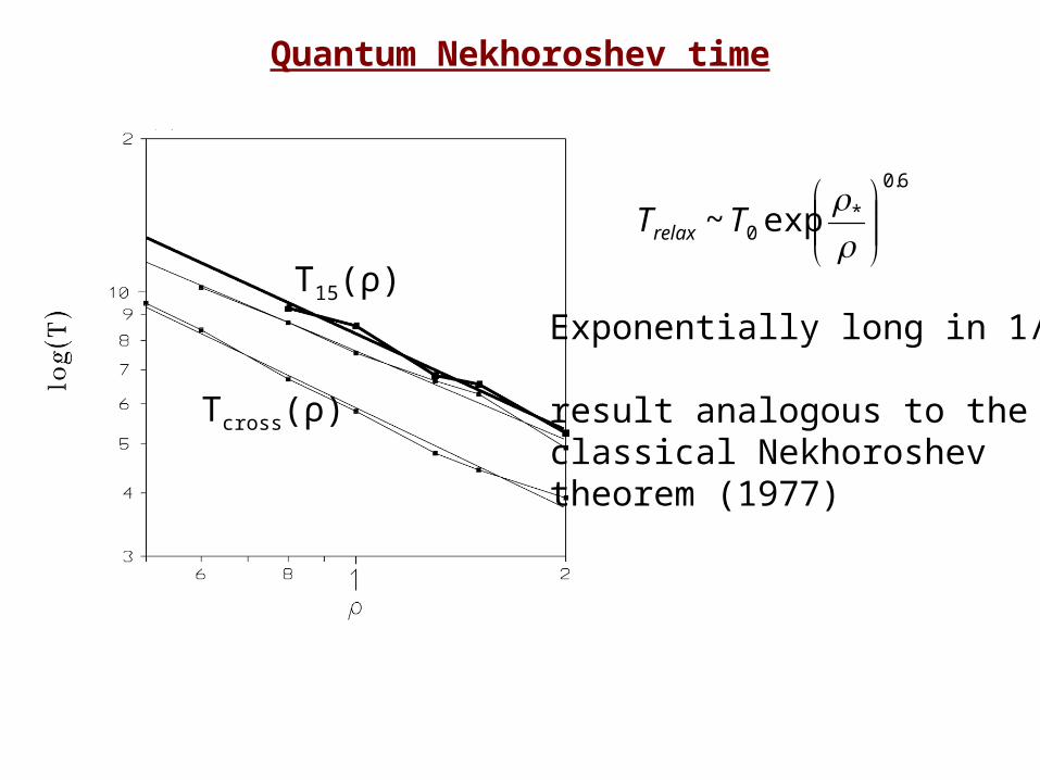
Quantum Nekhoroshev time

T15(ρ)

Tcross(ρ)

6.0

*0 exp~

TTrelax

Exponentially long in 1/ρ

result analogous to the classical Nekhoroshevtheorem (1977)

Possible explanation by quantum normal form theory?

(work in progress with N. Delis)

1) Write the Hamiltonian in terms of creation and anihilation operators:

3,1

2121,,,222111

2211

2121

2211)()(

2

1

2

1

lklk

kklllklk aaaaCaaaaH

2) Define near-identity unitary transformations: aj’=aj+O1(λ)+O2(λ2)+...bringing the Hamiltonian into normal form:

)',',','()',',','( 22112211 aaaaRaaaaZH

where Z has a vanishing commutator with its quadratic part.

3) quasi-coherent states are defined as eigenstates of the new anihilation operators. Their time stability is governed by a suitably defined norm ||R|| on the remainder. In Nekhoroshev theory: ||R||~exp(1/ε).

Normal form Remainder

Relaxation in non-completely chaotic regime?

III. Arrival and flight time df

in charged particle diffraction

The problem of time in quantum mechanics

(reviewed in Muga and Leavens 2000, and Muga et al. 2002)

1) Times are experimentally observed (e.g. TOF spectroscopy for heavy ions)

2) Time, however, is not an operator-valued observable (Pauli’s theorem). Furthermore, measurements in QM are considered to occur on instants of time

3) Several approaches, still ambiguous (and controversial)

- Kijowski (1972) arrival times distribution. For asymptotically free wave packets, it turns to be analogous to the classical flux approaxh

- Sum-over-histories approach (Yamada and Takagi 1992, based on works by Hartle, Gel-Mann, Griffiths and Omnes)

- POVMs (Anastopoulos and Savvidou 2006)

- Bohmian approach (Leavens): consistent and simple

A genuinely quantum phenomenon: diffraction of electrons through crystals

ingoing electronwavepacket

D: transverse quantum coherence length

l: transverse quantum coherence length

outgoing (radial) electron wavepacketin direction θ2

at t=2l0/v0

outgoing (radial) electron wavepacketin direction θ2

at t=2l0/v0

crystal: source of a radial wavepacket propagating from the center outwards

ρ=crystal number densityd=crystal thickness

Wavefunction modelling

Potential Eigenfunctions (in Born approximation)

sum over atomic nodes in the crystal

Final model

radial (Gaussian) wavepacket

Gaussian wavepacket

sum of phasors (produces diffraction pattern)

Outgoing wavefunction: fitting model

Fraunhofer factor(depending on the reciprocal lattice vector g)

at distances r<k0D2a/done has:

Seff~(ρD)1/2d

at large distances

)2/(sin4

),;(122

0

k

rgS

reff

Gaussianwavepacketpropagatingoutwards

Quantum current structure, separator and quantum vortices

central beam axis

D

separator: locus where |ψin|=|ψout|

Quantum trajectories:horizontal up to the point where separator is encounteredRadial outward afterwards

O(D)θ1

Ingoing term: exponential fall

Outgoing term:

power-law fall

22 /~ DRin e

rout /1~

`hard’ deflectionsdue to the approach to nodal point - X-point complexes

θ2

Bohmian trajectories(test numerically preservation of the continuity of the quantum flow)

Separator evolution and quantum vortices

Analytic approach to the locus of initial conditions leading to scattering in a particular angle θ

Arrival time distributions

t

l>>D

P(t)

Δt

Δt~max(l,D)/v0 (of order ~1psec for cold field emitter electrons)

t

D>>l

Time-of-flight difference for two scattering angles

where

Sum-over-histories (in semi-classical approximation):

),(1

4

||)()( 123

00

21

12

Fmv

eZZTT

Flux (Kijowski) approximation:

0)()( 12 TT (no trajectories, substract two asymptotic arrival time distributions)

Conclusions

1. Ordered Bohmian trajectories, lying in domains of analyticity of the quantum flow, are represented by series expansions in suitably defined small parameters

2. Chaos is generated by the motion of quantum vortices (ceation of nodal point - X-point complexes)

3. The quantum trajectories tend to avoid nodal points, but they are scattered chaotically by the latters’ associated X-points

4. Local Lyapunov characteristic exponents scale inversely proportionally to the vortex speed. No strict correlation of global chaos with the number of vortices.

5. In quasi-coherent quantum states, the approach to quantum equilibrium takes place within a timescale T~exp(1/ρ), where ρ is the phase-space distance of the state from the origin (`quantum Nekhoroshev theorem’)

6. The bohmian trajectories in scattering processes are very different from (semi-)classical trajectories. Scattering takes place in a separator domain at an O(D) distance from the central beam axis (D=transverse coherence length). Process ruled by an array of quantum vortices.

7. Arrival time distributions calculated with dBB theory show a characteristic double-peaked pattern with predictable parameters when D>>l (while Gaussian if l>>D)

8. Time-of-flight differences for different scattering angles scale as ΔΤ~D/v0. Very different than in other approaches (semi-classical: Τ~Z1Ze2/4πε0mv03, flux (Kijowski) ΔΤ=0).

Measurable?