Analytica Chimica Acta, 216 (1989) 307-319 Elsevier Science Publishers B.V., Amsterdam - Printed in The Netherlands

THE ROLE OF ANALYTICAL CHEMISTRY IN PROCESS QUALITY CONTROL

W.E. VAN DER LINDEN*, G. DE NIET and M. BOS

Laboratory for Chemical Analysis-CT, University of Twente, P.O. Box 217, 7500 AE Enschede (The Netherlands)

(Received 8th July 1988)

SUMMARY

The growing need for quality supervision and control in production processes is briefly outlined. After a summary of available process analytical devices, and a short discussion of their possibilities and limitations, an alternative approach is discussed. This approach is based on the development of a dynamic process model which allows on-line quality predictions to be made by means of so- called state estimators. The advantage is that it becomes possible to use quantities which give only indirect information about the product quality, but which are more readily accessible for continuous or on-line monitoring in earlier stages of the process.

At present, quality is a theme that is at the centre of interest. At least in part, this interest is stimulated by the tremendous success of the post-war development of Japanese industry based on new concepts of quality, quality- control and quality-assurance systems, including quality loops. These ideas have gradually penetrated manufacturing industries all over the world, includ- ing the chemical process industry and the food and pharmaceutical industries. Notions like “quality-give-away” and “off-spec production” may also be men- tioned in this respect. However, apart from economic reasons, technological reasons must also be mentioned as factors that have had a great influence. For all kinds of processes, ever-increasing demands are imposed on the quality of raw materials, intermediate products or semi-manufactured articles, and end- products, because their quality governs to a great extent their possible tech- nical use. In the chemical industry, improvement of product quality is often tantamount to improvement of the chemical composition, i.e., a decrease in the variation of this composition, a decrease in the amount of certain interfer- ing constituents or even the complete elimination of some components. Strik- ing examples can be found in the production of semiconductor materials and in the manufacturing of optical fibres for information transmission. In both cases, only exceptionally small amounts of certain compounds, within very narrow specified limits, can be tolerated.

These and other developments present a great challenge for analytical chem-

0003-2670/89/$03.50 0 1989 Elsevier Science Publishers B.V.

ists: not only do they have to deal with a continuously growing number of samples that have to be analyzed, they also have to provide more information per sample while, at the same time, improving the quality of the required in- formation in terms of better precision, lower limits of detection, faster availa- bility, etc. Up to now, the role of analytical chemists in the domain of quality control has been restricted mainly to the analysis of samples inside the labo- ratory; analytical chemists are rarely, if ever, seen on the production site itself. Analytical measurements in the production process proper are, in general, the responsibility of process or system engineers. At first sight, this may seem rather curious because these engineers seldom have sufficient knowledge of analytical chemistry to be able to guarantee the quality of the analytical mea- surements; they often use the signal delivered by the measuring instrument merely for the adjustment of operational parameters of the process, sometimes without much heed to the exact analytical interpretation and possible impli- cations of the measurements. The main reason for this undesirable situation is that process engineers are primarily responsible for the smooth running of a production process and are therefore more interested in aspects like robust- ness, maintenance and availability, or down-time of the analytical devices. However understandable this situation may be, further improvement of in- process quality control can be expected only if, on the one hand, process en- gineers will make the most of the available analytical knowledge while, on the other hand, analytical chemists are prepared to accept the challenge to develop methods and measuring techniques that have an inherent robustness which makes them suitable for use in an industrial environment. The actual design and construction of the analytical systems and instruments is the domain of specialists mostly employed by instrumentation companies.

In the next section, a brief summary is presented of the present status of process analytical devices. The conclusion reached is that the optimistic view of some authors with regard to general perspectives in the application of pro- cess analyzers, however justified for the longer term, is not justified in the short term. Therefore, another approach to quality control in (continuous) chemical processes is also discussed. This approach, which involves state estimations based on a dynamic model of the process that has to be controlled, allows the use of more easily measurable quantities.

PROCESS ANALYTICAL DEVICES

Although many process analyzers for in-process measurements of various chemical components are now commercially available, they are introduced only reluctantly in real process control. The main reason is that it is very difficult to meet the extremely high standards required with respect to reliability, ro- bustness, maintenance demand, etc., in particular when such devices have to form an integral part of an automatic control system [ 11. Process analyzers

309

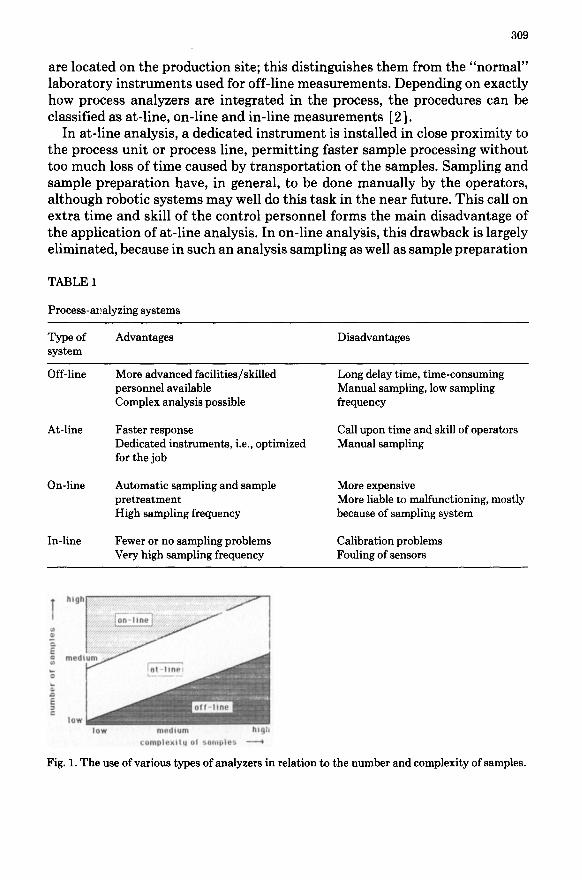
are located on the production site; this distinguishes them from the “normal” laboratory instruments used for off-line measurements. Depending on exactly how process analyzers are integrated in the process, the procedures can be classified as at-line, on-line and in-line measurements [ 21.

In at-line analysis, a dedicated instrument is installed in close proximity to the process unit or process line, permitting faster sample processing without too much loss of time caused by transportation of the samples. Sampling and sample preparation have, in general, to be done manually by the operators, although robotic systems may well do this task in the near future. This call on extra time and skill of the control personnel forms the main disadvantage of the application of at-line analysis. In on-line analysis, this drawback is largely eliminated, because in such an analysis sampling as well as sample preparation

TABLE 1

Process-analyzing systems

Type of system

Advantages Disadvantages

Off-line More advanced facilities/skilled personnel available Complex analysis possible

At-line Faster response Dedicated instruments, i.e., optimized for the job

On-line Automatic sampling and sample pretreatment High sampling frequency

In-line Fewer or no sampling problems Very high sampling frequency

Long delay time, time-consuming Manual sampling, low sampling frequency

Call upon time and skill of operators Manual sampling

More expensive More liable to malfunctioning, mostly because of sampling system

Calibration problems Fouling of sensors

Fig. 1. The use of various types of analyzers in relation to the number and complexity of samples.

310

TABLE 2

Survey of commercially available on-line process analyzers

Technique Gas Liquid Solid/ Major Minor Trace sludge

Spectrometric Ultraviolet/visible Fluorescence Chemiluminescence Infrared Near-infrared Mass spectrometry Nuclear magn. resonance (low field) Turbidity Opacity X-ray fluorescence

Electrometric pH,pIon Redox Conductometry Voltammetry Amperometry

02

Separation techniques Gas chromatography Liquid chromatography

Miscellaneous Polarimetry Refractometry Thermal conductivity Viscosity Paramagnetic measurements Density Calorimetry Wobbe index Melting point Flash point Cloud point Vapour pressure Particle size

+ + + + + + +

+ +

+ + + +

+ + +

+ +

+ +

+

+

+ + +

+

+ + +

+ +

+ +

+ + + + + + + + +

+ + +

+

+ + + +

+ + + +

+ + + + + +

+

+ + + +

+ +

are completely automated and form an integral part of the analyzing system. This sampling is mostly done by continuously draining part of the liquid or gas from the process unit or process line and leading the sample stream via a “fast

311

loop system” to the analyzer. Sampling is one of the major sources of problems in on-line analyzers. In principle, such problems can be avoided by using in- line analysis where a selective sensing device is placed in direct contact with the process solution or gas. But in practice, new difficulties may then arise because sample conditioning becomes impossible, calibration has to be done by removing the device from the process line or process unit, and fouling of the device can lead to base-line drift, decrease of the response or even complete disappearance of the signal.

The advantages and disadvantages of process-analyzing systems are briefly summarized in Table 1 in a very general way. Omitting in-line analysis because only a limited number of suitable sensors is available at present, the choice between off-line, at-line and on-line will depend on the sampling frequency imposed by the time constant of the process and on the complexity of the sam- ples as schematically illustrated in Fig. 1 [ 31. At present, on-line analyzing systems seem to be the most attractive for monitoring and control purposes provided that representative and reproducible sampling can be achieved. A survey of commercially available on-line analyzers is presented in Table 2. In spite of the large number of available analyzers of different types, very often none of them can be applied in a particular situation because of, for instance, lack of reliability, sampling problems (experts in this field estimate that about 75% of analyzer problems are related to difficulties with the sampling device), lack of selectivity, etc. In such cases, it is inevitable to accept measurements that only provide indirect information about the process and the quality of its end-products. However, in combination with a suitable model of the dynamic process, such indirect measurements may be suitable substitutes for direct measurements for predicting the ultimate product quality. In such cases, the development of a model for the dynamic process is an important starting point for properly planned quality control, as will be outlined in the next section.

APPROACH TO QUALITY CONTROL

The approach selected for the development of a system for quality control is defined as the “quality spiral” (Fig. 2). Several stages can be distinguished. In the first stage, an inventory is made of the process to establish which are the important products and process streams, how the process actually proceeds, which factors determine the quality, and which of these factors can be deter- mined by means of direct measurements. On the basis of this information, either a theoretical model is derived in which the remaining unknown param- eters have to be estimated by a limited number of suitably selected experi- ments, or a more empirical model is developed based on statistical techniques (e.g., correlation studies). The disadvantage of this latter approach is the rel- atively large number of experiments required and the lack of real insight into

12

quality spiral

Fig. 2. Schematic representation of the approach followed for the development of a system for quality control.

the process that they provide: they are, in fact, black-box or at the best grey- box models.

In the second stage, attention is focussed on the development of a state-space model or “state estimator”. Such a state estimator, derived from the original process model, should give optimal estimates of the state variables, even those that cannot be measured in a direct way. If there are no unknown variations in the process, and if the model is perfect, a special type of state-estimator, called an “observer”, can be used. On continuous measurement (observation of) the system, an observer enables the states to be estimated with gradually decreasing errors. However, models are normally not perfect and stochastic variations are to be expected. In such cases, an uncertainty in the estimate will remain even if the system is observed over a prolonged period of time; the model is then called a “filter”. For linear systems, Kalman was the first to describe suitable filter algorithms. These algorithms have a recursive character and yield a continuous update of the state estimates of the process when new analytical results become available [4]. Because not all measurements are equally helpful in eliminating the uncertainty about the state of the process, it makes sense to establish which measurements have the largest impact on the reliability of the estimate. Computer simulations with varying values of the various parameters can be used for this purpose. Subsequently, the desired accuracy and sampling frequency have to be determined. Gradually the third stage is reached. On the basis of all the information available with respect to type of measurement and/or components to be determined, the sampling fre- quency, and the precision required, a list can be composed with specifications of the extra information needed and a first selection can be made of the most

313

appropriate and useful type of analysis and analyzer. If required, some addi- tional simulations can be made with the characteristic values of the analyzer selected. In the final stage, algorithms for the automated regulation have to be developed and integrated in an integral control system.

The approach will be illustrated on the basis of a case study: the brine pu- rification process in the chloralkali industry for the production of pure sodium chloride [ 51

Brine purification: process description and model Figure 3 shows schematically the various units comprising the plant. Roughly

two steps can be distinguished: in the first step, all the magnesium ions and part of the calcium ions are eliminated from the brine in the form of Mg (OH), and CaS04*2H20, respectively. The hydroxide required is generated by the dissolution of hydrated lime, Ca ( 0H)2, and the sulfate is supplied by the brine and the recirculating mother liquor (mainly sodium sulfate) from the evapo- ration unit. In the second step, the remaining calcium ions are eliminated by the formation of calcium carbonate. The carbonate required stems from the

product

Fig. 3. Schematic representation of a brine purification process.

314

fast reaction between the$arbon dioxide (flue gas) that is introduced and the hydroxide present, or may be added as sodium carbonate. In the process, these two sections can also be discerned: the first one comprises three reactors in series and a clarifier; the second one comprises two reactors and again a clar- ifier. The sludges from the two clarifiers are combined and led to a Dorr-type thickener. Part of the sludge from the first clarifier is ground and this material is fed into the first reactor as seed crystals. The reactors in the first section provide the necessary residence time; each can be described as an ideal contin- uously stirred tank reactor (CSTR). The first reactor in the second section is a gas reactor, and the second reactor in this section can also function as such. Recycling loops are indicated by arrows in the figure.

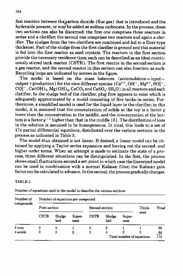
The model is based on the mass balances (accumulation=input- output+production) for the nine different species (Ca2+, OH-, Mg2+, SO:-, CO;-, Ca( 0H)2, Mg(OH)2, CaCO, and CaS0,*2H20) in all reactors andeach clarifier. In the sludge bed of the clarifier, plug flow appears to exist which is adequately approximated by a model consisting of five tanks-in-series. Fur- thermore, a simplified model is used for the liquid layer in the clarifier; in this model, it is assumed that the concentration of solids at the top is a factor g lower than the concentration in the middle, and the concentration at the bot- tom is a factor g -’ higher than that in the middle [ 61. The distribution of ions in the solution is assumed to be homogeneous. In total, this leads to a set of 174 partial differential equations, distributed over the various sections in the process as indicated in Table 3.

The model thus obtained is not linear. If desired, a linear model can be ob- tained by applying a Taylor-series expansion and leaving out the second- and higher-order terms. When an attempt is made to estimate the state of a pro- cess, three different situations can be distinguished. In the first, the process shows small fluctuations around a set-point in which case the linearized model can be used in combination with a normal Kalman filter; the Kalman gain factor can be calculated in advance. In the second, the process gradually changes

TABLE 3

Number of equations used in the model to describe the various sections

Number of Number of equations per compound compounds

First section Second section Thick- Total ener

CSTR Sludge Super- CSTR Sludge Super- bed nate bed nate

5 ions 3 5 1 2 5 1 1 90

4 solids 3 5 2 2 5 2 2 84 Total number of equations 174

315

with time but the variations are small and the states lie between some well defined set-points; again the Kalman gain factor can be calculated in advance as the average of the factor obtained for the various set-points involved, for the estimation of the state of the process the non-linearized process model is used. In the third situation, the process changes considerably with time, which precludes the use of the linearized process model and makes it necessary to recalculate the Kalman gain factor after each measurement; this form of filter is called the extended Kalman filter.

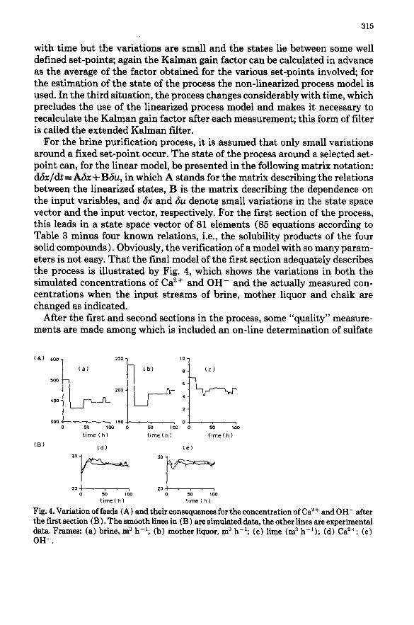
For the brine purification process, it is assumed that only small variations around a fixed set-point occur. The state of the process around a selected set- point can, for the linear model, be presented in the following matrix notation: d&/dt = A& + Bdu, in which A stands for the matrix describing the relations between the linearized states, B is the matrix describing the dependence on the input variables, and 6x and 6~ denote small variations in the state space vector and the input vector, respectively. For the first section of the process, this leads in a state space vector of 81 elements (85 equations according to Table 3 minus four known relations, i.e., the solubility products of the four solid compounds). Obviously, the verification of a model with so many param- eters is not easy. That the final model of the first section adequately describes the process is illustrated by Fig. 4, which shows the variations in both the simulated concentrations of Ca2+ and OH- and the actually measured con- centrations when the input streams of brine, mother liquor and chalk are changed as indicated.

After the first and second sections in the process, some “quality” measure- ments are made among which is included an on-line determination of sulfate

0 50 100 0 50 100 0 50 100

time(h) tlme(hl time(h)

(8) Cd) (e)

time(h)

Fig. 4. Variation of feeds (A) and their consequences for the concentration of Ca2+ and OH- after the first section (B) . The smooth lines in (B ) are simulated data, the other lines are experimental data. Frames: (a) brine, m3 h-‘; (b) mother liquor, m3 h-l; (c) lime (m3 h-l); (d) Ca2+; (e) OH-.

[ 71. For the subsequent step in the salt production process, i.e., the evapora- tion unit, it is of great importance that the sulfate concentration is kept con- stant. The variations in the sulfate concentrations are mainly caused by the reactions taking place in the first section. Therefore, attention was focussed on this section. In order to determine which process parameters have a major influence on the quality of the product, a procedure called noise propagation was used. This means that on each of the separate state variables in the model, noise is introduced and the effect on the different estimated state variances is calculated. In Table 4 the results for the normal set-point conditions of the process are summarized. The results of this procedure look rather disappoint- ing in the sense that there is hardly any mutual influence and that the varia- tions in the composition of the various feeds determine to a great extent the final composition and quality of the product. So, in this case, quality control can be achieved by good control of the feeds. However, analytically, some prob- lems arise because the various process solutions are close to saturation or even supersaturated; this causes big sampling problems. Moreover, measurements of flow rate are rather inaccurate for the same reason. At present, special at- tention is being given to these aspects. In the case of sulfate, for instance, it is not the absolute flow rate but the ratio of the flow rates of the brine and mother liquor that is of importance in order to keep the sulfate concentration constant, thus in both streams accompanying ions which do not participate in the reac- tions of the purification process are monitored. Potassium ions seem to be good pilot ions for this purpose.

In the example discussed above, further simulations indicated that no im- provement could be expected by combining quality measurements (which are generally available at low frequency only) with more frequent measurements of other process parameters that are more easily accessible.

De Niet [ 51 and de Niet and van Heusden [ 81, however, have shown that in

TABLE 4

Effect of 5% noise introduced in the first reactor on the respective concentrations at the outlet of the first section (in % )

Ion measured at the outlet of the first section

Ions corrupted with 5% noise in the first reactor

Ca2+ OH- Mg2+ co;- soq-

Ca2+ 9.0 0.9 OH- 0.5 6.8 ,p+a 22 436 104 co;- 2.8 0.03 42.6 so:- 0.1 10.5

a [ Mg2+ ] is very low at the end of the first section.

317

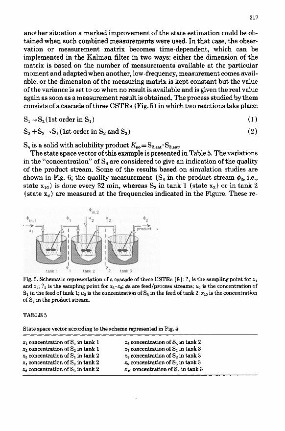
another situation a marked improvement of the state estimation could be ob- tained when such combined measurements were used. In that case, the obser- vation or measurement matrix becomes time-dependent, which can be implemented in the Kalman filter in two ways: either the dimension of the matrix is based on the number of measurements available at the particular moment and adapted when another, low-frequency, measurement comes avail- able; or the dimension of the measuring matrix is kept constant but the value of the variance is set to oo when no result is available and is given the real value again as soon as a measurement result is obtained. The process studied by them consists of a cascade of three CSTRs (Fig. 5) in which two reactions take place:

S,-rSz(lst order in S,)

S, + S3 +S, ( 1st order in $4, and S,)

S, is a solid with solubility product K,, = SP,sat*SB,saV

(1)

(2)

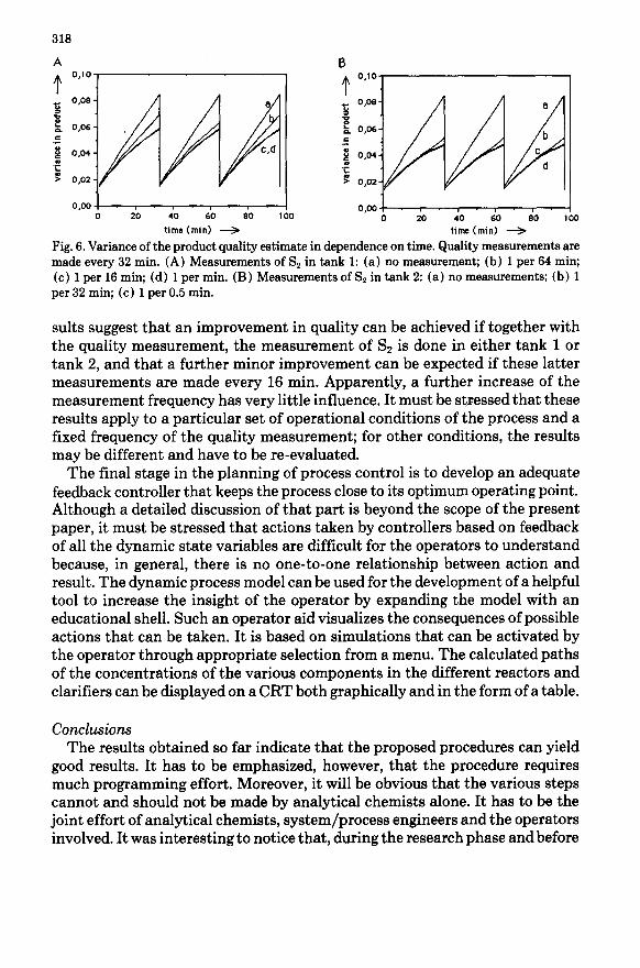
The state space vector of this example is presented in Table 5. The variations in the “concentration” of S, are considered to give an indication of the quality of the product stream. Some of the results based on simulation studies are shown in Fig. 6; the quality measurement (S, in the product stream &, i.e., state xiO) is done every 32 min, whereas Sz in tank 1 (state xq) or in tank 2 (state x4) are measured at the frequencies indicated in the Figure. These re-

‘in 2

‘in.1 *, llU2’ *2

+ oduct x

tank I I tank 2 2 tank 3

Fig. 5. Schematic representation of a cascade of three CSTBs [8]: ?I is the sampling point for x1 and x2; ?* is the sampling point for x3-x6; $s are feed/process streams; u1 is the concentration of S, in the feed of tank 1; u2 is the concentration of S, in the feed of tank 2; xl0 is the concentration of S, in the product stream.

TABLE 5

State space vector according to the scheme represented in Fig. 4

n, concentration of S, in tank 1 x6 concentration of S, in tank 2 xp concentration of S, in tank 1 x7 concentration of S, in tank 3 x3 concentration of S, in tank 2 x8 concentration of S, in tank 3 x4 concentration of S, in tank 2 x9 concentration of 5s in tank 3 x5 concentration of S, in tank 2 xl0 concentration of S4 in tank 3

318

H 0,08- B k O,Oh-

.5

2 0,04- .z k > 0,02-

2 o,oe- a z k 0,06- .c

C p 0,04- .I d k > 0.02

0.00, , , , ,

0 20 40 60 80 100 0,oo

;w b

0 20 40 60 80 100

time (mid -_j time (mid +

Fig. 6. Variance of the product quality estimate in dependence on time. Quality measurements are made every 32 min. (A) Measurements of Sz in tank 1: (a) no measurement; (b) 1 per 64 min; (c) 1 per 16 min; (d) 1 per min. (B) Measurements of S, in tank 2: (a) no measurements; (b) 1 per 32 min; (c) 1 per 0.5 min.

sults suggest that an improvement in quality can be achieved if together with the quality measurement, the measurement of S2 is done in either tank 1 or tank 2, and that a further minor improvement can be expected if these latter measurements are made every 16 min. Apparently, a further increase of the measurement frequency has very little influence. It must be stressed that these results apply to a particular set of operational conditions of the process and a fixed frequency of the quality measurement; for other conditions, the results may be different and have to be re-evaluated.

The final stage in the planning of process control is to develop an adequate feedback controller that keeps the process close to its optimum operating point. Although a detailed discussion of that part is beyond the scope of the present paper, it must be stressed that actions taken by controllers based on feedback of all the dynamic state variables are difficult for the operators to understand because, in general, there is no one-to-one relationship between action and result. The dynamic process model can be used for the development of a helpful tool to increase the insight of the operator by expanding the model with an educational shell. Such an operator aid visualizes the consequences of possible actions that can be taken. It is based on simulations that can be activated by the operator through appropriate selection from a menu. The calculated paths of the concentrations of the various components in the different reactors and clarifiers can be displayed on a CRT both graphically and in the form of a table.

Conclusions The results obtained so far indicate that the proposed procedures can yield

good results. It has to be emphasized, however, that the procedure requires much programming effort. Moreover, it will be obvious that the various steps cannot and should not be made by analytical chemists alone. It has to be the joint effort of analytical chemists, system/process engineers and the operators involved. It was interesting to notice that, during the research phase and before

319

any of the steps discussed above had been implemented, the quality of the products improved. Merely the increased interest of other people in the per- formance of the plant, and the awareness that careful operation can enhance quality, was an important incentive for the operators.

REFERENCES

1 W.E. van der Linden, Kern.-Kemi, 15 (1988) 459. 2 J.B. Callis, D.L. Illman and B.R. Kowalski, Anal. Chem., 59 (1987) 624A. 3 F. Laurijs, lecture presented at “Het Instrument” exhibition, Utrecht, May 1988. 4 S.D. Brown, Anal. Chim. Acta, 181 (1986) 1. 5 G. de Niet, Ph.D. Thesis, University of Twente, 1988 (in Dutch). 6 B. Roffel, Polytech. Tijdschr., Procestechniek, 32 (1977) 583 (in Dutch). 7 H. van den Dolder, Anal. Chim. Acta, 190 (1986) 25. 8 G. de Niet and A.R. van Heusden, in preparation.