Carnegie-Rochester Conference Series on Public Policy 49 (1998) 245-263 North-Holland

The robustness of identified V A R conclusions about money*

A c o m m e n t

H a r a l d U h l i g

CentER, Tilburg University

and

CEPR

T h e key idea A central question in macroeconomics is the effect of monetary policy on

output. The recent VAR literature seems to have reached a consensus, that

(*) For every reasonable identification of the VAR, the mone- tary policy shocks account for a small share of the forecast error variance of output.

Jon Faust examines the claim (*) by proposing and performing a sensitivity analysis with respect to all "reasonable" identification schemes, calculating the extreme bounds of the forecast error variance in the spirit of learner (1983). "Reasonable" here means, that the impulse response functions be- have "reasonable," i.e., that they replicate the conventional wisdom taught in most intermediate macroeconomics textbooks:

(**) After a contractionary monetary policy shock, the federal funds rate goes up (liquidity effect), while real GDP, prices, and reserves go down.

Despite the efforts by many researchers to directly exploit institutional details for disentangling the contemporaneous timing of shocks, (**) is usually im- plicitely or explicitely imposed in many VAR identification exercises as well.

*I am grateful to B. Bernanke and I. Mihov for providing me with their data set. The address of the author is Harald Uhlig, CentER, Tilburg University, Postbus 90153, 5000 LE Tilburg, The Netherlands, e-maih uhlig~kub.nl, fax: +31-13-4663066, phone: +31-13-4663104, home page: http://center.kub.nl/staff/uhlig.

0167-2231/98/$ - see front matter © 1998 Elsevier Science B.V. All rights reserved. PII: S0167-2231 (99)00010-X

As Ben Bernanke half-jokingly observed at this conference, he "wouldn't have been invited," if his identification had failed to reproduce (**). Thus, the VAR literature does not really (yet) answer the question as to whether (**) is true or not. Instead, that literature assesses the quanti tat ive magnitudes, given (**), as a maintained hypothesis. Therefore, (**) is a sensible start ing point for Jon Faust 's analysis as well.

A VAR in reduced form can be written as

Yt = B(1)Yt-1 ÷ B(2)Yt-2 + ... ÷ B(0Yt-i ÷ ut, t = 1, ..., T (1)

In order to identify monetary policy shocks and other economically inter- pretable shocks, one needs to disentangle u~ into " s t r u c t u r a r ' shocks vt:

u, = Av , (2)

I

Assuming E[v~v~] = I , the only restriction on A is

= E[utu't] = A E [ v t v ~ ] A ' = A A ' (3)

Since the focus here is solely on monetary policy shocks, the following defi- nition is useful (see Uhlig (1997)):

D e f i n i t i o n 1 The vec tor a C R m is called an i m p u l s e vec to r , i f there

is s o m e m a t r i x A , so that A A I = ~ and so that a is a co lumn o f A .

The set of all impulse vectors can be obtained by rotation (see Faust 's paper or Uhlig (1997)) for details. The impulse vector yields the instantaneous impulse response of all variables to the structural shock associated with that vector. The full impulse response function is then easily calculated. The s tandard identification problem can be phrased as the problem of finding an impulse vector representing a contractionary monetary policy shock. With (**), that impulse vector needs to have the "correct" signs: negative in all entries except the federal funds rate. Faust proposes the following procedure:

1. Find the set of all impulse vectors with "'correct" signs. Possibly re- strict tha t set further via, e.g., restrictions on impulse responses at later horizons.

2. Calculate the range of the fraction of variance in real GDP nine years after the shock, accountable for by impulse vectors in tha t set.

He finds tha t the range is too large to support (*) conclusively, with some- what stronger evidence offered in larger VARs.

246

H o w to th ink a b o u t the paper There is a difference between asking whether monetary policy shocks could have large effects on output and (*). "Neutralists" might argue that mone- tary policy shocks have no real effects, as long as they are not too dramatic. Indeed, the recent VAR literature seems to offer some empirical support for that view. Monetarists (as well as Keynesians) on the other hand believe that monetary policy is a powerful tool. But even if it is, (*) can be true, if monetary policy shocks are typically small. Ben Bernanke's (1996) analogy on page 72 makes this clear: "[N]uclear explosions account for approximately 0 percent of output variation in the U.S. economy over the past thirty years, but that fact is not informative about what would happen if nuclear weapons were actually used." Indeed, central banks are probably not keen on rocking the boat. Alan Blinder (1997) writes on page 15: "While I never saw a single case of a central banker succumbing to the temptation that so worried Kyd- land and Prescott, I often witnessed central bankers sorely tempted to deliver the policy that the markets expected or demanded." These two quotes nicely express the current consensus, supporting (*).

In light of this view, how can one interpret Jon Faust 's finding that mon- etary policy shocks may explain up to 91% of the variance of the nine-year- ahead prediction error in real GDP? Could it be that there is little variance in real GDP nine years out, so that small monetary policy shocks are sufficient. to explain all of it? And if so, what would this imply for the consensus in the real business-cycle literature, that 70% of cyclical variations (measured as HP-filtered standard deviations) are due to technology shocks? Faust favors instead the interpretation that there is little we have been able to learn from VARs about (*), even though (*) may well be correct. I agree with that assessment, but the other interpretations offer intriguing possibilities, too.

The paper is clearheaded. It rightly stresses the importance of directly looking at impulse responses in order to bring the "conventional wisdom" to bear on the issue: this is my point of view too (see Uhlig (1997) and also Dwyer (1997)). Faust's paper is an important contribution to the literature. But there are also a number of questions which need to be addressed. Let me turn to them now.

A r e l a rge r s y s t e m s really more conc lus ive? Faust concludes that evidence for (*) can be found in larger systems, but not in smaller systems. Is that a reasonable conclusion? I do not think so: the difference is mild at most. Figure 1 provides a graphical comparison of the numbers obtained in Table 1 and Table 2 in Faust. The downward shift for the larger model seems to be there, but it is by no means dramatic enough to allow a clear distinction. There may also be theoretical reasons to believe

247

that the maximal importance any single shock can play in a system goes down as the number of variables goes up. As Faust explains, without the sign restriction, the maximum variance due to a single shock is given by the maximal eigenvalue of the matrix collecting the variances and covariances of the n components of the nine-year-ahead prediction error for real GDP due to the n shocks in some base identification. Should we generally expect this eigenvalue to increase or decrease as n increases? In any case, in order to judge whether the decline in the larger system is really due to a greater informativeness of the sign restrictions in larger systems or whether it is due to the decrease of maximal importance of any single shock, a comparison of the largest eigenvalues as benchmarks would have been useful.

Table 1:

Variables VAR innov, first diff.

real GDP (Y) GDP deft. (P)

comm. prices (CP) total reserves (TR)

nonborr, res. (NBR)

45% 52% 47% 48% 60%

46% 44% 37% 53% 62%

P, NBR 30% 27% ... + Y 15% 14%

P, CP, TR, NBR 9% 7% ... + Y 4% 5%

Notes: This table shows how often we see the federal funds rate move in the opposite direction of the variables listed above. The calculations here as well as for the rest of the paper are based on the Bernanke-Mihov data set, containing monthly observations for 1965-1994. The first column used the innovations calculated from a VAR at the MLE, whereas the second column uses first differences after removing means.

Finally, Leeper, Sims, and Zha (1996) have already argued for consider- ing more than just one monetary policy shock in larger systems. That is plausible: sterilized exchange-rate interventions are probably different from a general tightening. But if there are several monetary policy shocks, they may, in combination, account for a larger fraction of the variance in real GNP.

How often do we see conventional monetary policy shocks? While the reduced-form innovations ut are always combinations of several shocks, one might nonetheless expect ut to frequently exhibit the sign re- strictions implied by (**), if monetary policy shocks are a dominant part of the time series movements. Is that true? Table 1 provides an admittedly

248

His

togr

am o

f 50

% Q

uant

iles:

Tab

le 1

ve

rsus

Tab

le 2

t,O

',,0

35

30

C

• ~

2

5

.E

20

"-

15

0 '.-

10

o.

5 0

• T

ab

le 1

• T

ab

le 2

~ ~,

~" ©

~

" ~,

~" ,8

" ~;

" ,~

" ~'

",~,

..

Per

cent

of

vari

ance

exp

lain

able

F

igur

e 1 :

this

is

a hi

stog

ram

of

the

num

bers

in

Tab

les

1 an

d 2

in t

he F

aust

pap

er,

i.e.,

the

max

imal

fra

ctio

n of

GN

P p

redi

ctio

n er

ror

vari

ance

exp

lain

able

wit

h a

mon

etar

y sh

ock,

usi

ng v

ario

us m

odel

spe

cifi

cati

ons

and

rest

rict

ions

. The

lig

hter

bar

s ar

e fo

r th

e sm

alle

r m

odel

, i.e

., T

able

1, w

here

as t

he d

ark

bars

are

for

the

lar

ger

mod

el,

i.e.

Tab

le 2

. T

he d

iffe

renc

es b

etw

een

thes

e tw

o ta

bles

is

not

grea

t.

crude assessment. While the federal funds rate moves fairly often in the op- posite direction of any one of the other five variables, all these other variables move in the same direction at the same time in only about five percent of all cases. Thus, it is rare to see a conventional monetary policy shock dom- inating the one-step-ahead prediction error u, (see also Leeper, Sims, and Zha (1996)). If we are to believe that they can nonetheless explain a large fraction of the movements in real GDP, then what is going on?

Is 9 smal l er t h a n ce ? Faust decomposes the prediction error for GDP nine years into the future. Perhaps an explanation for his findings is that we are fairly uncertain what happens that far out. To examine this, I proceeded in the following manner.

1. Using the Bernanke-Mihov data set, I ran a Bayesian vector-auto- regression (BVAR) with an off-the-shelf Normal-Wishart prior, de- scribed in the Appendix.

2. I took 100 hundred draws from posterior for the reduced-form VAR, i.e., for the coefficient matrices B j , j = 1, ..., l and E. For each draw from posterior, I generated 500 draws of impulse vectors with a "correct" sign, using roughly a uniform distribution on the appropriate piece of the ellipsoid.

3. Of these 500 draws, I kept the one which explains the highest fraction of real GDP variance eight years out (I picked eight years rather than nine to add some variety).

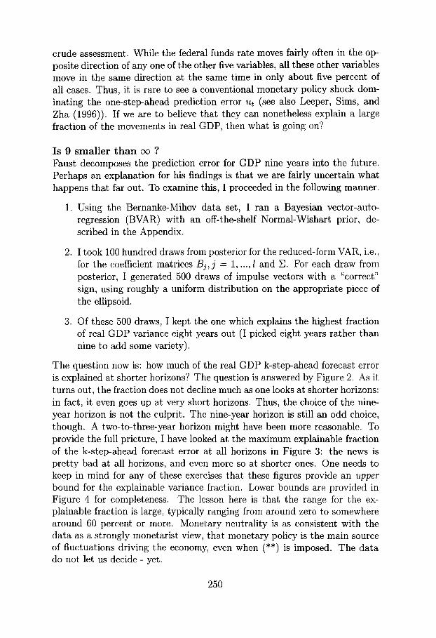
The question now is: how much of the real GDP k-step-ahead forecast error is explained at shorter horizons? The question is answered by Figure 2. As it turns out, the fraction does not decline much as one looks at shorter horizons: in fact, it even goes up at very short horizons. Thus, the choice of the nine- year horizon is not the culprit. The nine-year horizon is still an odd choice, though. A two-to-three-year horizon might have been more reasonable. To provide the full pricture, I have looked at the maximum explainable fraction of the k-step-ahead forecast error at all horizons in Figure 3: the news is pret ty bad at all horizons, and even more so at shorter ones. One needs to keep in mind for any of these exercises that these figures provide an upper

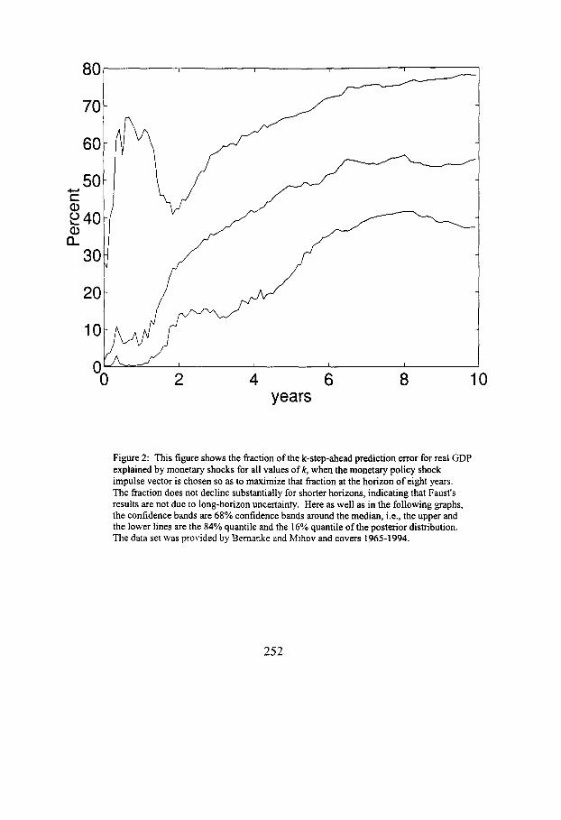
bound for the explainable variance fraction. Lower bounds are provided in Figure 4 for completeness. The lesson here is that the range for the ex- plainable fraction is large, typically ranging from around zero to somewhere around 60 percent or more. Monetary neutrality is as consistent with the data as a strongly monetarist view, that monetary policy is the main source of fluctuations driving the economy, even when (**) is imposed. The data do not let us decide - yet.

250

A r e t h e i m p u l s e r e s p o n s e s rea l ly " r e a s o n a b l e " ? Rethinking what has been done so far; one notices that (**) has not really been imposed in its full force yet: so far, I have simply insisted that the impulse vector has the correct signs on impact. However, (**) should properly be interpreted as a somewhat persistent property. With that interpretation, there is indeed a problem, as can be seen from Figure 5. The federal funds rate typically falls back to zero or even reverses sign practically immediately following the shock. So, what would happen if we insist that all impulse responses keep the correct sign for up to a year following the shock?

Faust looks into this a bit in his Tables 1 and 2, but really not very much: the restriction is imposed only for one series and only at one point in the future. To investigate this further, I have proceeded as above, but out of the 500 draws of the impulse vector drawn for a given realization of the reduced-form VAR posterior, I have kept only those which satisfied the impulse response inequality restrictions implied by (**) at all horizons for up to one year. This turned out to be a suprisingly stringent demand: for about two-thirds of the reduced-form draws, I did not get a single impulse vector draw satisfying the inequality constraint. In those cases I threw away the reduced-form posterior draw, effectively imposing the sharp prior that there must exist an impulse vector satisfying (**). The maximal explainabl(~ fraction of the k-step-ahead prediction error for real GDP is plotted in Figure 6. Clearly, the explainable fraction of the variance has dropped substantially, as one can see when comparing the numbers in this figure with the numbers in Figure 3. If there are impulse vectors satisfying the inequality restrictions, keep the one which maximizes the fraction of the real GDP prediction error variance eight years into the fugure: the impulse responses from these draws are given in Figure 7.

What is remarkable is the fact that the federal flmds rate falls back to zero or even reverses sign practically immediately as soon as it is allowed to, i.e., following the 12 months it is restricted to be positive. Because of this and because I had to throw away about two-thirds of my reduced-form posterior draws because of the impossibility to satisfy (**) for a full year, I drew the conclusion that the data really do not like (**) with respect to the federal funds rate. (**) seems to be only consistent with the data if one is to accept a rather quick reversal of the rise in the federal funds rate. One of the following three reasons may provide an explanation:

1. The liquidity effect is very short-lived and followed by a Fisher effect within less than one year: the decrease in the inflation rate leads to a quick decrease in nominal short-term interest rates. This seems to be Faust's point of view who professes to be "skeptical regarding the

251

8O

70

6O

5 0 C

~40 £

30 i

20

I I I I

2 4 6 8 years

10

Figure 2: This figure shows the fraction of the k-step-ahead prediction error for real GDP explained by monetary shocks for all values of k, when the monetary policy shock impulse vector is chosen so as to maximize that fraction at the horizon of eight years. The fraction does not decline substantially for shorter horizons, indicating that Faust's results are not due to long-horizon uncertainty. Here as well as in the following graphs, the confidence bands are 68% confidence bands around the median, i.e., the upper and the lower lines are the 84% quantile and the 16% quantile of the posterior distribution. The data set was provided by Bernanke and Mihov and covers 1965-1994.

252

1 0 0 1 . . . .

0..

80

60

40

20

O 0 I I I I 2 4 6 8

years 10

Figure 3: This figure shows the maximal fraction of the k-step-ahead predic- tion error for real GDP explainable by a monetary shock for each value of k. I.e., in contrast to Figure 2, the monetary policy shock impulse vector is chosen to maximize the explainable fraction at each given horizon k and not at the horizon of eight years.

253

8 , , , ' O

0.7

0.6

0.5 v "

o 0 . 4 (D

12. 0.3

0.2

I I I I

2 4 6 8 years

10

Figure 4: This figure shows the minimal rather than the maximal fraction of the k-step-ahead prediction error for real GDP explainable by a monetary shock for each ~ lue of k. It is constructed in a manner similar to Figure 3. As one can see, monetary neutrality and thus even extreme versions of (*) cannot be ruled out either.

254

Impulse response for real GDP

E 2 CD n

-0.51-

-1 0 2 4 6 8

years

Impulse response for GDP price defL 0 . . . .

-0.2[ ~ ~ -0.4 _ S

~-0.6~ \ \

~. -0.8

_~ 2 i F ~

-1.4~

lO

2 4 6 8 years

Impulse response for Comm. pnce ind.

ol

a.-2 t ~ ~ - -

i i

o 2 4 6 8 10 years

Impulse response for Total Reserves

0.6 J

0.4

~ 0.2! ~. o'

-0.21

-0.6! 2 4 6 8 10

years

Impulse response for Nonborr. Reserv.

years

Impulse response for Fed. Funds Rate

0.4 • i

Lo.2 i

-060 2 4 6 8 10 years

Figure 5: Impulse responses to a contract ionary monetary policy shock, when the impulse vector is chosen so as to maximize the explainable fraction of real GDP variance at the horizon of eight years. Note in particular, tha t the federal funds rate typically falls back to zero or even reverses sign practically immediately following the shock.

255

6O

5ol 40

o30 13_

20

10

0~ ~

I I I I

2 4 6 8 years

10

Figure 6: This figure shows the maximal fraction of the k-step-ahead predic- tion error for real GDP explainable by a monetary shock for all values of k, when the impulse responses are restricted to be of the correct sign for up to a year following a monetary contraction. Except for this additional restriction, it is constructed similar to Figure 3.

256

0.2,

~ - 0 . GI o n~-0.4

-0.6

-0.~

Impulse response for real GDP

f f

2 4 6 8 10 years

Impulse response for GDP price deft .

~ 2 4 6 8 10 years

Impulse response for Comm. price ind. 0.5

o

-0.5

c -1

-2

-2.5

2 4 6 8 10 years

Impulse response for Total Reserves 0.6

0.41

0.21

~.-0.2

-0.6

0.61

2 4 0 8 10 years

Impulse response for Nonborr. Reserv.

0.41

021

g.-0.2

-0.6

2 4 6 8 10 years

Impulse response for Fed. Funds Rate 0.6r

0.2

-0.2

-0.4 3 2 4 6 8 10 years

Figure 7: Impulse responses to a contractionary monetary policy shock, when the impulse vector is chosen so as to maximize the explainable fraction of real GDP variance at the horizon of eight years, subject to the constraint of "correct" signs for up to one year. Note in particular that the federal funds rate falls back to zero or even reverses sign practically immediately following the year in which it was constrained to be positive by construction.

257

persistence of the liquidity effect on interest rates."

2. Monetary policy follows a feedback rule, quickly undoing a monetary policy shock and possibly even overshooting to the other side.

. The contractionary monetary policy shock has a recessionary effect, which by itself leads to a lowering of the federal funds rate. Thus, even if the federal funds rate returns to zero, this indicates tightness.

No one of these three reasons sounds like the kind of thing we typically tell our undergraduates, but I think we probably should. If we want to stick to the conventional view embodied in (**), it is in serious need of updat- ing. Or, perhaps, (**) should be called into question itself: perhaps, the real effect on output of monetary policy shocks is murkier in the data than conventional wisdom as well as some artifacts of the VAR literature would lead us to believe. Further investigations are called for.

A r e t h e r e su l t s r ea l ly d i f fe ren t f r o m resu l t s one w o u l d ge t us ing iden t i f i ca t ions u sed in t h e l i t e r a t u r e ? Once the inequality constraints are imposed for a full year in Figures 6 and 7, should one have a d~j£ vu feeling? Examine Figure 8, in which monetary policy is identified as the innovation in nonborrowed reserves ordered fourth in a Cholesky decomposition. It does not look much different from Figure 7. The variance of the real GDP prediction error in Figure 9 does not look dra- matically different from Figure 6 either. The numbers rather than the shape matter in that comparison: the median estimate in Figure 6 for the out- put variation explainable by monetary policy shocks is usually about twenty percent with peaks up to thirty percent, while it varies between about five and thirty percent in Figure 9. Remember, that Figure 6 was constructed by maximizing that variance share at each given horizon k! Twenty percent is also roughly the fraction, which Cochrane (1994) found in other contexts. One has to conclude that the differences from the usual findings really are not dramatic.

Put differently: once the conventional view (**) is imposed properly, the results one gets from Faust's analysis are pretty much what one would have found anyhow, and are thus perfectly consistent with the literature findings. We should not be more uncertain about (*) than we have been before.

Thus, what, if anything, did we learn from Faust's analysis? We did not learn that the claim for (*) is grossly overstated in the literature, as his paper seems to suggest. Rather, we get a deeper understanding about the identi- fication restriciton implicit in much of the VAR literature. We understand more deeply whether (*) is a fragile claim or not. It does not seem to be. That is progress. We also understand better that (**) is in serious need of

258

Impu lse response for real G D P o.2

o,1

o

~ -0 .1

I~- -0.2

-0.3

-0.4

--o.s o 2 4 6 8 lO

0.4

years

Impulse response for GDP price deft.

0.2

0

~ -0.2

~-0.4 -0.6

-0.8~

_11 o

years

Impulse response for Comm, price ind. 0.5 • - - ~ __

o

-0.5

(D 2-1.5 oJ CL -2

-2.5

-3

-3.5

Impulse response for Nonborr. Reserv. l r

0.5

0 2 4 6 8 10 years

Impulse response for Total Reserves 0.E

0.E

0.4

~ 0.2

"0.6 f --0.8 2 4 6 8 10

years

Impulse response for Fed. Funds Rate

0.2 ,

g ,

,!

o 2 , 6 8 1o - 0 % - 2 ;, o ~ l o years years

Figure 8: Impulse responses to a contractionary monetary policy shock, when the monetary policy shock is identified as the fourth sho9ck in a Cholesky decomposition, ordering the variables as real GDP, GDP deflator, commod- ity prices, nonborrowed reserves, total reserves, federal funds rate. Note that the impulse responses do not look very different from Figure 7.

259

0 , , , ,

40

.,-3O ¢ -

£

n 20

10

2 4 6 8 y e a r s

' " " ~ 1

10

Figure 9: Fraction of the k-step-ahead prediction error for real GDP ex- plained by monetary policy shocks, identified as the innovation in nonbor- rowed reserves ordered fourth in a Cholesky decomposition.

260

updating.

C o n c l u d i n g r e m a r k s Faust 's paper is clearheaded and an important contribution to the litera- ture. Given my own statements in Uhlig (1997), I obviously share the view to directly look at impulse responses in order to bring the "conventional wisdom" (**) to bear on the issue of the influence of monetary policy. His paper provides a useful and important technique. When properly impos- ing the conventional wisdom (**) by restricting the impulse responses for a full year, however, the fraction of variance explainable by monetary policy shocks does not seem to be much different than what one would get out of a standard identification exercise, e.g., using innovations in nonborrowed re- serves ordered fourth in a Cholesky decomposition as monetary policy shocks. Faust 's claim that (*) is a fragile conclusion is therefore overstated. While examining these issues, I also found that the conventional wisdom is in need of some serious updating: following a contractionary monetary policy shock, the data seem to strongly suggest that the federal funds rate return to zero very quickly within a few months or even overshoot in the other direction. More work is needed on the empirical as well as the theoretical front. As a suggestion, it could be fruitful to investigate further the links between the- ory and facts, when taking into account that monetary policy tries to follow market expectations, as Blinder (1997) has suggested.

Appendix For convenience, we collect here the main tools for estimation and inference. We use a Bayesian approach since that allows for a conceptually clean way of drawing error bands for statistics of interest such as impulse responses, (see Sims and Zha (1995) for a clear discussion on this point). Furthermore, imposing the sign restrictions is conceptually easier in the Bayesian frame- work. In much of the VAR literature, one sees occasional small violations of these sign restrictions, and there is a tendency to tolerate them on tile grounds that they are probably not significant. In a Bayesian context as the one used here, they literally do not make sense under (**), as a potentially "true" draw of the reduced-form VAR specification should not, e.g., predict prices to go up after a few months following a contractionary shock.

Using monthly data, we fixed the number of lags at 1 = 12 as in Bernanke and Mihov (1996a, 1996b). Stack the system (1) as

Y = XB + u (4)

where X t = [Yt'_I,Yt'_2,...,Yt'_tI',Y = [YI, ..., Y T I ' , X = [ X X 1 , . . . , X T ] ' , u = [Ul, ..., UT] ~ and B = [B0) , ..., Bl]' . To compute the impulse response to an

261

impulse vector a, let a = [a', 01,re(t-i)]' as well as

F = Ira(t-l) 0m(Z-1),m

and compute rk,j = (Fka)j, l = 0, 1, 2, ... to get the response of variable j at horizon k. The variance of the k-step-ahead forecast error due to an impulse vector a is obtained by simply squaring its impulse responses. Summing again over all a3, where aj is the j-th column of some matrix A with AA' = E, delivers the total variance of the k-step-ahead forecast error.

We assume that the ut's are independent and normally distributed. The MLE for (B, E) is given by

= ( X ' X ) - I x ' y , ~ = T ( Y - X/3)'(Y - X/3) (6)

Our prior aNW, O as well as the benchmark posterior aT for (B, F., a) belongs to the Normal-Wishart family, whose properties are further discussed in Uhlig (1994). A proper Normal-Wishart distribution is parameterized by a "mean coefficient" matrix /3 of size k x rn, a positive definite "mean covariance" matrix S of size m x m as well as a positive definite matrix N of size 1 x 1 and a "degrees of freedom" real number u _> 0 to describe the uncertainty about (B, E) around (/3, S). The Normal-Wishart distribution specifies that E -1 follow a Wishart distribution Win(S- i /u , u) with E[E -1] = S -1, and that, conditional on E, the coefficient matrix in its columnwise vectorized form, vec(B), follows a Normal distribution N(vec(B), E ® N- l ) . Furthermore, we have a flat density with respect to the parameterization a.

To use these distributions in practice, one needs to be able to draw from them. That should be easy for the normal distribution part. To draw from the Wishart distribution Wm(S-1/u , u), use, e.g., E = (R * R') -1, where R is a m x u matrix with each column an independent draw from a Normal distribution N(0, S - l / u ) with mean zero and variance-covariance matrix S -1 .

Proposition 1 on p. 670 in Uhlig (1994) states that if the prior is described by/30, No, So and u0, then the posterior is described by /3T, NT, ST and UT, where

UT = T + uo

NT = N0 + X'X

/~T = NTI(No/~o -b X'X/~)

= "°So + + 1 ( $ _ o),NoN :lx, x ( _ Bo) /]T /IT /]T

We use a "weak" prior, and use No = 0, P0 = 0, So and/30 arbitrary. Then, B T = ]~, ST : ~ , YT : T , N T = X'X, which is also the form of the posterior used in the RATS manual for drawing error bands (see example 10.1 in Doan (1992)).

262

References

Bernanke, B.S., (1996). Discussion of 'What Does Monetary Policy Do?' (Eds.) E.M. Leeper, C.A. Sims and T. Zha, Brookings Papers on Economic Activity, series 2, 69-73.

Bernanke, B.S. and Mihov, I., (1996a). Measuring Monetary Policy, NBER working paper no. 5145, June 1995, updated as INSEAD Discussion paper 96/74/EPS/FIN, 1996.

Bernanke, B.S. and Mihov, I., (1996b). The Liquidity Effect and Long- run Neutrality: Identification by Inequality Constraints, draft, INSEAD and Princeton, 1996.

Blinder, A.S., (1997). Distinguished Lecture on Economics in Government: What Central Bankers Could Learn from Academics and Vice Versa, Journal of Economic Perspectives, 11: (2): 3-19.

Cochrane, J., (1994). Shocks, Allan Meltzer and Charles Plosser, (eds.,) Carnegie-Rochester Conference Series on Public Policy, 41: Amsterdam, North-Holland.

Doan, T.A., (1992). RATS User's Manual, Version 4, Estima, 1800 Sherman Ave., Suite 612, Evanston, IL 60201.

Dwyer, M., (1997). Dynamic Response Priors for Discriminating Structural Vector Autoregressions, draft, UCLA.

Leamer, E.E., (1983). Let's Take the Con Out of Econometrics, American Economic Review, 73: 31-43.

Leeper, E.M., Sims, C.A., and Zha, T., (1996). What Does Monetary Policy Do? Bookings papers on Economic Activity, series 2, 1- 63.

Sims, C.A. and Zha, T., (1995). Error Bands for Impulse Responses, Federal Reserve Bank of Atlanta Working paper no. 6.

Uhlig, H., (1994). What Macroeconomists Should Know About Unit Roots: a Bayesian Perspective, Econometric Theory, 10: 645- 671.

Uhlig, H., (1997). What Are the Effects of Monetary Policy? Results From an Agnostic Identification Procedure~ draft, Tilburg University.

263