The Risk Anomaly Tradeoff of Leverage*

Malcolm Baker Harvard Business School and NBER

Mathias F. Hoeyer

University of Oxford

Jeffrey Wurgler NYU Stern School of Business and NBER

March 17, 2016

Abstract

Higher-beta and higher-volatility equities do not earn commensurately higher returns, a pattern known as the risk anomaly. In this paper, we consider the possibility that the risk anomaly represents mispricing and develop its implications for corporate leverage. The risk anomaly generates a simple tradeoff theory: At zero leverage, the overall cost of capital falls as leverage increases equity risk, but as debt becomes riskier the marginal benefit of increasing equity risk declines. We show that there is an interior optimum and that it is reached at lower leverage for firms with high asset risk. Empirically, the risk anomaly tradeoff theory and the traditional tradeoff theory are both consistent with the finding that firms with low-risk assets choose higher leverage. More uniquely, the risk anomaly theory helps to explain why leverage is inversely related to systematic risk, holding constant total risk; why leverage is inversely related to upside risk, not just downside risk; why numerous firms maintain low or zero leverage despite high marginal tax rates; and, why other firms maintain high leverage despite little tax benefit.

                                                                                                                         * For helpful comments we thank Hui Chen, Sam Hanson, Thomas Philippon, and seminar participants at the American Finance Association, Capital Group, George Mason University, Georgetown University, the Ohio State University, NYU, the New York Fed, the University of Tokyo, the University of Amsterdam, the University of Miami, the University of Utah, and USC. Baker and Wurgler also serve as consultants to Acadian Asset Management. Baker gratefully acknowledges financial support from the Division of Research of the Harvard Business School.

1

I. Introduction

According to traditional capital structure theory, adding leverage increases the risk and

cost of equity but, in the absence of other frictions, does not change the overall weighted average

cost of capital. As long as equity and debt markets are integrated, and therefore price risk the

same way, the division of risk between equity and debt is irrelevant.

Empirical research in asset pricing has called into question how the stock market, in

particular, prices risk and return. For example, the Capital Asset Pricing Model (CAPM) predicts

that the expected return on a security is proportional to its systematic risk, i.e., market beta. The

“risk anomaly” is the empirical pattern that stocks with higher beta or volatility have tended to

earn lower returns, not higher returns, both on a risk-adjusted basis and sometimes even on an

unadjusted basis. Put simply, the fundamental risk-return relationship in the stock market has

historically been flat, if not inverted.

The risk anomaly was originally put forth in the 1970s and is now the subject of a

burgeoning empirical and theoretical literature. Contributions include Fama and French (1992),

Falkenstein (1994), Ang, Hodrick, Ying, and Zhang (2006), Blitz and van Vliet (2007), Baker,

Bradley, and Wurgler (2011), and several others. The anomaly appears in long samples,

including international samples. A number of these papers consider the findings to be evidence

of mispricing as opposed to a somewhat backwards misspecification of risk. We do not provide

another attempt to resolve this issue but rather, in the spirit of Stein (1996), who considers

rational capital budgeting in the presence of capital market mispricing, we study how capital

structure should be set in the presence of a risk anomaly.

The basic idea of the risk anomaly theory of leverage is that firms with relatively low risk

assets—and hence underpriced equity, all else equal—may want to rely disproportionately on

2

debt to take advantage of the anomaly. We develop and test this idea in three steps. First, we

measure the risk anomaly in equity and corporate debt returns. Second, we model optimal

leverage in the presence of the risk anomaly. Third, we return to the data and explore the model’s

main prediction of an inverse relationship between leverage and systematic risk and test other

predictions that distinguish it from the standard tradeoff theory.

We measure the risk anomaly in a large sample of CRSP returns data. Consistent with

prior results, a one-unit increase in equity beta is associated with lower beta-adjusted stock

returns – that is, lower realized cost of equity – of around 5% per year. But because capital

structure irrelevance depends on market integration, not a rational tradeoff between risk and

return, we extend these to confirm that the anomaly, at least in an integrated fashion, does not

extend to debt markets.

Our model of optimal leverage illustrates a simple tradeoff. It assumes no frictions other

than a risk anomaly in equity. This contrasts with traditional tradeoff theories, which generate an

interior optimum by assuming one friction to limit leverage on the high side and another to limit

it on the low side. The intuition of the risk anomaly tradeoff is as follows. Under the anomaly,

risk is overvalued in equity but not in debt.2 Ideally, then, to minimize the cost of capital, the

firm concentrates risk in equity. A firm will always want to issue as much riskless debt as it can.

This lowers the cost of equity by increasing its risk without any “inefficient” transfer of risk to

debt. But, as debt becomes risky, further increases in leverage have a cost. Shifting overvalued

risk in equity securities to fairly valued risk, or simply less overvalued risk, in debt increases the

cost of capital. For firms with high-risk assets, this cost is high even at low levels of leverage.

For firms with very low risk assets, this cost remains low until leverage is high. We prove that

                                                                                                                         2 This is for convenience. The intuition and qualitative results would be identical if the risk anomaly is merely weaker in debt markets.  

3

there is an interior optimum leverage ratio that is inversely related to asset beta. Calibrations

using the empirical size of the anomaly suggest that the value gains from exploiting the tradeoff

appropriately, or the losses from not doing so, can be substantial.

We find strong empirical support for the main prediction that leverage is inversely related

to asset beta. We start with a firm-specific measure of asset beta, but to avoid the mechanical

negative link between leverage and the firm’s asset beta that arises from unlevering its equity

beta we conduct most of the analysis with industry asset beta. The explanatory power of asset

risk variables is largely separate from the explanatory power of profitability, asset tangibility,

market-to-book assets, size, and marginal tax rates.

Clearly, the risk-leverage prediction overlaps with a central prediction of the traditional

tradeoff theory with financial distress costs, including dynamic generalizations implicating asset

beta such as Schwert and Strebulaev (2014), so neither approach can claim immediate credit for

this empirical result. We turn to other aspects of the data to establish at least an incremental role

for the risk anomaly theory.

For starters, a prominent shortcoming of the traditional tradeoff theory is the low-

leverage puzzle. Graham (2000) and others have pointed out that hundreds of profitable firms,

with high marginal tax rates, maintain literally zero leverage. Conversely, a number of other

profitable firms maintain quite high leverage despite no tax benefit. The traditional tradeoff

theory has difficulty with these facts, but the inverse relationship between risk and leverage

suggests how the risk anomaly tradeoff could help. If low leverage firms find that the tax benefit

of debt is less than the opportunity cost of transferring risk to lower-cost equity, low leverage

may be optimal even in the presence of additional frictions; a minor transaction cost of issuance

could drive some firms to zero leverage. Meanwhile, low asset risk firms with no tax benefits of

4

debt still need a substantial amount of it to take advantage of the anomaly. Hence, while it is not

immediately apparent which theory explains the middle range of leverage—a reasonable position

is that both are at play—the extremes are more easily accommodated by the risk anomaly theory.

Increasingly complex variants of the traditional theory also have trouble explaining some

results. For example, optimal leverage may depend inversely on systematic risk because higher

asset beta, all else equal, reflects the market state and increases in the present value of the costs

of financial distress when it is likelier to occur. Almeida and Philippon (2007) make this general

argument, while Shleifer and Vishny (1992) suggest clustered asset fire sales as a mechanism.

This explanation has an empirical weakness and a more fundamental conceptual weakness.

The empirical weakness is that the cost or risks of financial distress is a “downside” risk.

If this is what is limiting leverage for high asset risk firms, we would expect “downside beta,”

not “upside beta,” to drive the negative leverage-risk relationship. Under the risk anomaly

theory, in contrast, upside beta is just as relevant. And, empirically, we find that upside beta is, if

anything, the stronger empirical link to leverage.

The conceptual weakness is that the traditional tradeoff theory, with rational asset

pricing, cannot explain both the notion that systematic risk measured by beta increases the

present value of the costs of financial distress and the asset pricing evidence that systematic risk

measured by beta is not priced. It seems highly desirable to have a single paradigm to explain

both asset pricing facts and leverage patterns, and the risk anomaly tradeoff offers one.

Section II reviews the literature on the risk anomaly and measures it in our data. Section

III presents a model of optimal leverage under a risk anomaly. Section IV contains empirical

tests. Section V concludes.

5

II. The Risk Anomaly

In this section we give some background on the anomaly and then estimate its size in our

own data. Based on a broad view of the evidence, the anomaly is a sufficiently robust pattern to

justify an exploration of its normative implications for capital structure.

A. Background

Over the long run, riskier asset classes have earned higher returns in U.S. markets. Small

stocks have outperformed large caps, which have outperformed corporate bonds, which have

outperformed long-term Treasuries, and so on (Ibbotson Associates (2012)). Our interest,

however, is the evidence that the historical risk-return tradeoff within the stock market is flat or

inverted. While the Capital Asset Pricing Model (CAPM) predicts that the expected return on a

security is proportional to its systematic risk (beta), stocks with higher beta (or idiosyncratic risk)

have tended to earn lower returns, particularly on a risk-adjusted basis.

The risk anomaly is present across stock markets and sample periods. Black (1972),

Black, Jensen, and Scholes (1972), Haugen and Heins (1975), and Fama and French (1992)

noted the relatively flat relationship between expected returns and beta in the U.S. Subsequently,

Falkenstein (1994) and Ang, Hodrick, Ying, and Zhang (2006) have emphasized the magnitude

and robustness of the anomaly. Blitz and van Vliet (2007), Ang et al. (2009), and Baker, Bradley,

and Taliaferro (2013) confirm its presence within developed markets and Blitz, Pang, and van

Vliet (2013) document it in emerging markets.

The magnitude of the anomaly is substantial. Baker, Bradley, and Taliaferro (2013) find

that a dollar invested in a low quintile beta portfolio of U.S. stocks in early 1968 grows to $70.50

by the end of 2011, a while dollar invested in a high beta portfolio grows only to $7.61. In a

6

sample of up to 30 developed equity markets over a shorter period beginning in 1989, these

figures are $6.40 and $0.99. We estimate the anomaly’s size in more useful units below.

Several explanations for the anomaly have been developed. Investors may have an

irrational preference for volatile or skewed investments, due to overconfidence, as in Cornell

(2008), or lottery preferences, as in Kumar (2009), Bali, Cakici, and Whitelaw (2011) and

Barberis and Huang (2008). Other investors may simply categorize stocks together and neglect to

price differences in risk, as in Barberis and Shleifer (2003). Leverage-constrained investors who

seek maximum returns from beta risk must buy high beta stocks directly as opposed to forming a

levered portfolio of low beta stocks (Black (1972) and Frazzini and Pedersen (2014)).

Moreover, sophisticated investors may have trouble exploiting and eliminating the

anomaly. Fund managers may prefer high-beta assets themselves because the inflows to

performing well are greater than the outflows to performing poorly (Karceski (2002)) or because

they are rewarded for beating the market, which presumably has a positive risk premium, on a

non-beta-adjusted basis (Brennan (1993) and Baker et al. (2011)). More generally, short-selling

constraints inhibit sophisticated investors’ ability to exploit an overpricing of high-beta stocks

(Hong and Sraer (2012)).

A relatively open question is the existence or size of a similar anomaly in debt markets.

As we discuss below, this is important for corporate finance implications. The most recent

evidence is Houweling, van Vliet, Wang, and Beekhuizen (2014), who find that short-maturity

corporate bonds issued by low risk firms have slightly higher beta-risk-adjusted returns. A

significant difference for our purpose is that their betas are with respect to the corporate bond

market. Fama and French (1993) report that stock market betas are practically identical for bond

portfolios of various ratings and conclude that different risk factors describe returns in the stock

7

and bond markets, i.e., the markets are not integrated. Baele, Bekaert, and Inghelbrecht (2009)

find that the magnitude and even the sign of the correlation between stock index and government

bond returns are highly unstable. Nonetheless, we are not aware of a formal test for an integrated

risk anomaly, so we conduct a simple one.

The risk anomaly challenges not just the CAPM—a convenient but not strictly necessary

assumption of traditional capital structure theory—but any framework where risk and expected

return are positively related. There is, of course, a vast literature in asset pricing that aims to

identify measures of risk that perform better than beta, with the implicit notion that beta is not a

meaningful risk to the representative investor. In light of the robust evidence and reasonable

explanations for the anomaly, however, this paper follows several others and takes the view that

it reflects inefficient asset pricing, not misspecification of risk.

B. Measuring the Anomaly

We focus on estimating the magnitude of the anomaly as an input to later calibrations.

We also establish that it is primarily an equity market phenomenon. Should there happen to be

an identical anomaly across the equity and debt markets, then, as suggested above, the cost of

capital would vary pathologically with asset risk but in a way that managers could not control

with financial structure. It is therefore important to rule this out.

We use a linear specification for risk anomaly in equity

re = β −1( )γ + rf +βrp (1)

and debt

rd = βd −βd( )γd + rf +βdrp (2)

8

where rf is the risk free rate, rp is the market risk premium, βd is average debt beta, and γ. <= 0

measures the size of the anomaly in that market.3 Risk-adjusted expected returns decrease

linearly with risk: Securities with one additional unit of risk relative to their market average have

–γ. lower risk-adjusted returns. Otherwise, the CAPM holds.4

Figure 1 shows three potential scenarios involving low risk anomalies. The light solid

line shows the theoretical security market line. Panel A illustrates an integrated risk anomaly in

which γ = γd < 0. While this scenario has investment implications—overinvestment relative to

the CAPM prediction for firms with high asset beta and vice-versa—it has none for capital

structure. If the two markets are integrated then the Modigliani-Miller theorem is preserved and

(with the minor modification that the weighted average of equity and debt betas is one) the cost

of capital is simply

WACC = ere + 1− e( )rd = βa −1( )γ + rf +βarp (3)

which is independent of the chosen capital structure e. Panel B shows the case of a risk anomaly

in equities and correctly priced debt. Here, γ < γd = 0. Panel C shows the case of low risk

anomalies in both equity and debt with the empirically relevant case of  γ < γd < 0 (although there

is no theoretical reason why the anomaly could not be greater in debt).

We first estimate the relationship between equity returns and beta using data from

January 1931 through December 2012 from the Center for Research in Securities Prices (CRSP)

data. We include all industries. We compute results for the 45 years (540 months) since January

1968, when the number of stocks in the beta portfolios becomes large and which approaches the

                                                                                                                         3 These apply to any firm i but we suppress the relevant subscripts on betas and costs of capital. We also suppress the subscript e on the equity beta and gamma.

4 Following typical practice, we will compute betas with respect to the stock market, but conceptually all that matters is that we use a common market for equity and debt.  

9

beginning of our Compustat leverage sample, as well as the full sample of 82 years (984 months)

since January 1931. We use CRSP value-weighted market returns for CAPM-based analyses and

add the Fama-French SMB and HML factors for their 3-factor model. We use a minimum of 24

months and a maximum of 60 months of returns to estimate market betas for each stock, and then

form value-weighted and equal-weighted bottom 30%, middle 40%, and top 30% beta portfolios.

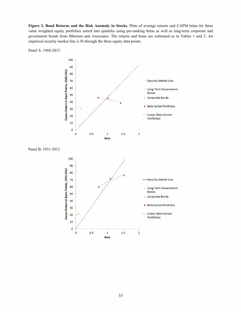
Tables 1 and 2 show the raw returns, factor slopes, and alphas for each portfolio

weighting, risk-adjustment model, and sample period combination. Figure 2 also plots the alphas

against CAPM beta. The lack of a meaningful (positive) relationship between risk and return in

equities is evident.

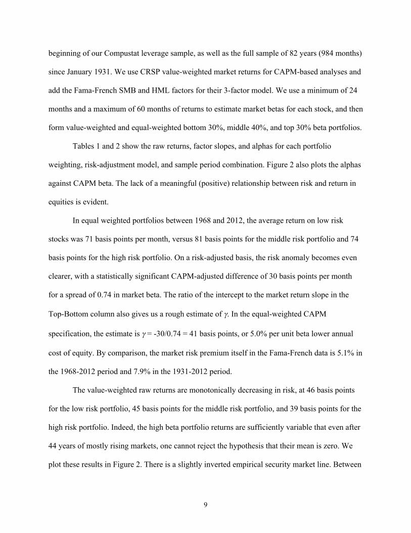
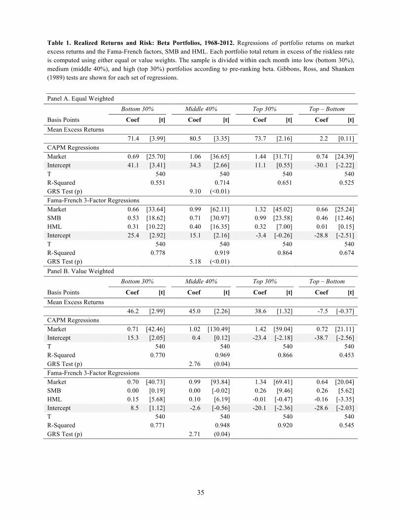
In equal weighted portfolios between 1968 and 2012, the average return on low risk

stocks was 71 basis points per month, versus 81 basis points for the middle risk portfolio and 74

basis points for the high risk portfolio. On a risk-adjusted basis, the risk anomaly becomes even

clearer, with a statistically significant CAPM-adjusted difference of 30 basis points per month

for a spread of 0.74 in market beta. The ratio of the intercept to the market return slope in the

Top-Bottom column also gives us a rough estimate of γ. In the equal-weighted CAPM

specification, the estimate is γ = -30/0.74 = 41 basis points, or 5.0% per unit beta lower annual

cost of equity. By comparison, the market risk premium itself in the Fama-French data is 5.1% in

the 1968-2012 period and 7.9% in the 1931-2012 period.

The value-weighted raw returns are monotonically decreasing in risk, at 46 basis points

for the low risk portfolio, 45 basis points for the middle risk portfolio, and 39 basis points for the

high risk portfolio. Indeed, the high beta portfolio returns are sufficiently variable that even after

44 years of mostly rising markets, one cannot reject the hypothesis that their mean is zero. We

plot these results in Figure 2. There is a slightly inverted empirical security market line. Between

10

the high and low risk portfolios, the intercepts relative to the theoretical security market line

differ by 39 basis points against a spread of 0.72 in market beta. For the Fama-French three

factor model these results are the same or stronger. Finally, a Gibbons, Ross, Shanken (1989) test

for the joint significance of the intercepts rejects the null in all specifications.

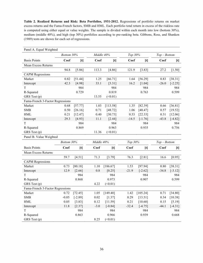
The story since 1931 is similar. The anomaly is not immediately apparent in raw returns,

although even after 81 years there is no statistically significant difference between the return on

high and low risk portfolios. The risk-adjusted returns again reveal the anomaly. As before, there

is an even stronger risk anomaly with respect to the Fama-French model, apparently from netting

out the prominent small cap (SMB) and value (HML) effects in the high beta portfolio.

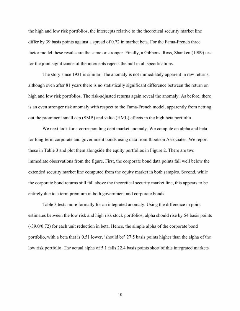
We next look for a corresponding debt market anomaly. We compute an alpha and beta

for long-term corporate and government bonds using data from Ibbotson Associates. We report

these in Table 3 and plot them alongside the equity portfolios in Figure 2. There are two

immediate observations from the figure. First, the corporate bond data points fall well below the

extended security market line computed from the equity market in both samples. Second, while

the corporate bond returns still fall above the theoretical security market line, this appears to be

entirely due to a term premium in both government and corporate bonds.

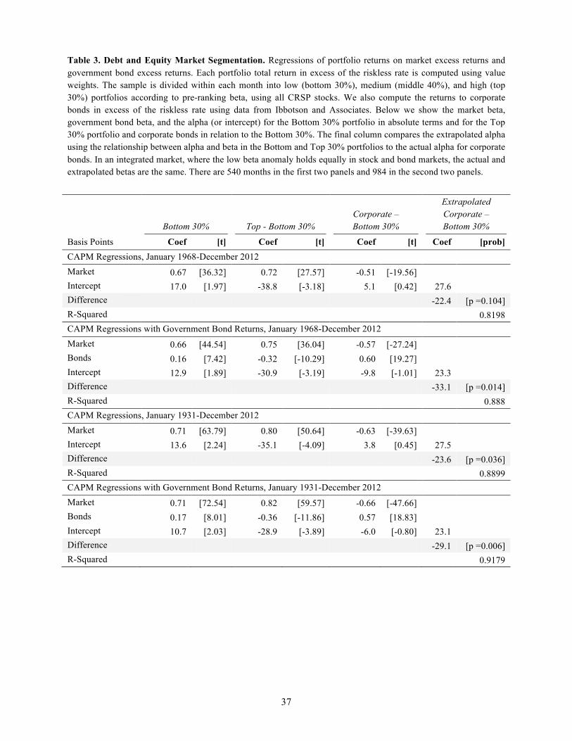
Table 3 tests more formally for an integrated anomaly. Using the difference in point

estimates between the low risk and high risk stock portfolios, alpha should rise by 54 basis points

(-39.0/0.72) for each unit reduction in beta. Hence, the simple alpha of the corporate bond

portfolio, with a beta that is 0.51 lower, ‘should be’ 27.5 basis points higher than the alpha of the

low risk portfolio. The actual alpha of 5.1 falls 22.4 basis points short of this integrated markets

11

target. The actual and extrapolated alphas are far enough apart that we can reject integration at

roughly a 10% level.5

A portion of the return on corporate bonds during this period reflects falling inflation, not

an integrated anomaly. With this in mind, we also control for the term premium on government

bonds in the second panel. Baker and Wurgler (2013) find that there is a statistically strong link

between bond returns and the cross-section of stock returns. The low risk stock portfolio is much

more exposed to government bond returns than is the high risk stock portfolio. This turns out to

explain only a small portion of the risk anomaly in stocks, however. By contrast, exposure to

government bond returns explains the entire alpha on corporate bonds. The alpha on corporate

bonds is now 9.8 basis points lower than the low risk stock portfolio, while it ‘should be’ 23.3

basis points higher. The gap of 33.1 basis points is highly statistically significant. Over the full

history, when the performance of government bonds was more modest, we reject integration

even more strongly.

In short, while there is a link between government bonds and low risk stocks, there is

otherwise little evidence of a common risk anomaly across debt and equity markets. This means

reducing the risk of corporate equity by substituting equity for corporate bonds would not have

left the overall cost of capital unchanged. Put in terms of Figure 1, the data are most consistent

with Panel B or perhaps Panel C with a modest risk anomaly in debt markets. As these two cases

have qualitatively similar conclusions for optimal capital structure, we will assume that debt is

correctly priced in the model.

                                                                                                                         5 To compute a p-value we draw from a multivariate normal distribution using the OLS estimates and covariances for the coefficients in the first three columns. For each of 10,000 draws, we compare the actual and extrapolated alpha. A one-tailed p-value of 0.095, for example, indicates that approximately 950 of the random draws feature an actual alpha that is higher than the extrapolated alpha.

12

III. The Risk Anomaly and Leverage

This section outlines a static model of optimal capital structure with no frictions other

than a risk anomaly in equity. There are no taxes, transaction costs, issuance costs, incentive or

information effects of leverage, or costs of financial distress or bankruptcy. Unlike other tradeoff

models, which require one tradeoff to limit leverage on the low side and another to limit it on the

high side, this single mechanism drives an interior optimum. The central prediction we are

working toward is that firms with high asset beta will prefer low leverage; the natural benefit

they acquire from the low beta anomaly deteriorates quickly with leverage, while low beta firms

will pursue high leverage in order to better capture it.

We discuss this prediction in more detail at the end of this section as a lead-in to the

empirical work. We hypothesize that the risk anomaly mechanism contributes explanatory power

to the cross-section of leverage both within the normal range and in the extremes that highlight

some shortcomings of the standard tradeoff model: namely, the hundreds of firms that maintain

zero or almost zero debt despite clear tax benefits and ability to pay, and the numerous other

firms that maintain high debt despite low or zero marginal tax rates.

A. A Risk Anomaly Tradeoff Theory

The main assumption is the existence of a linear anomaly in equity and no anomaly in

debt, i.e., roughly consistent with our previous empirical results. This is the case of Panel B in

Figure 1 and corresponds to γ < γd = 0 in terms of Equations (1) and (2). A less important

assumption is that the CAPM holds up to the risk anomaly in equity, but any model with a

stronger risk anomaly in equity will lead to the same qualitative conclusions. By assuming

sufficient conditions for the CAPM to hold in rational markets, we can develop comparative

statics using the familiar transfers of beta risk from equity to debt as leverage increases.

13

When there is a risk anomaly in equity, so that γ is nonzero, the weighted average cost of

capital depends not only on asset beta but on leverage:

WACC(e) = ere + 1− e( )rd = rf +βarp + βa −1( )γ − 1− e( ) 1−βd( )γ , (3)

where e is the ratio of equity to firm value and debt beta, without any further loss of generality, is

a function of leverage and the underlying asset risk. The second to last term (the asset beta minus

one times γ) is the uncontrollable reduction (increase) in the cost of capital that comes from

having high-risk (low-risk) assets. The last term is the controllable cost of having too little

leverage.

The optimal capital structure minimizes this last term, by satisfying the first order

condition for e. With the further assumption of a differentiable debt beta, for a given level of

asset beta the optimal capital ratio e* satisfies:

−γ 1−βd e*(βa ),βa⎡⎣ ⎤⎦+ 1− e

*(βa )⎡⎣ ⎤⎦∂βd e

*(βa ),βa⎡⎣ ⎤⎦∂e

⎧⎨⎪

⎩⎪

⎫⎬⎪

⎭⎪= 0

(4)

or in terms of optimal debt beta

β*d e*(βa ),βa⎡⎣ ⎤⎦=1+ 1− e

*(βa )⎡⎣ ⎤⎦∂βd e

*(βa ),βa⎡⎣ ⎤⎦∂e

.

Interestingly, the optimum leverage does not depend on the size of the risk anomaly. This is

somewhat of a technicality, however. If there were other frictions associated with leverage, such

as taxes or financial distress costs, the anomaly’s size would be relevant.

Under the assumption of a linear risk anomaly as expressed in Equation (1), the optimum

leverage will be an interior solution as follows. With zero debt, the asset beta is equal to the

equity beta and equation (3) reduces to

14

WACC(1) = rf +βarp + βa −1( )γ .

With a first-order Taylor approximation around e =1, we find that even marginal debt will

decrease the cost of capital:

WACC(e) ≈WACC(1)+ (1− e)λ <WACC(1) .

If the company is fully debt financed, the debt beta becomes equal to the asset beta and Equation

(3) reduces to that of the traditional WACC formula without the risk anomaly. This establishes

that the optimum leverage must be an interior solution to equation (4).

Observation 1: Firms will increase debt to minimize cost of capital. The first order

condition cannot be satisfied if the debt beta is zero. At a zero debt beta, the left side of Equation

(4) is positive. In other words, issuing more equity at the margin will raise the cost of capital.

At first blush, this would seem to deepen the low leverage puzzle. One might ask why

nonfinancial firms do not increase their leverage ratios further to take advantage of the risk

anomaly: It is initially unclear how the low leverage ratios of nonfinancial firms represent an

optimal tradeoff between the tax benefits of interest and the costs of financial distress, much less

an extra benefit of debt arising from the mispricing of low risk stocks.

The answer contained in Equation (4) is that many low leverage firms—e.g. the

stereotypical unprofitable technology firm—already start with a high asset beta or overall asset

risk. Their assets are already quite risky at zero debt. Even at modest levels of debt, meaningful

amounts of risk are transferred from equity to debt.

To further our understanding of optimal debt levels, a characterization of the dynamics

underlying transfer of risk from equity to debt with increasing levels of leverage is necessary. A

leading candidate for the functional form of debt betas is the Merton (1974) model. Merton uses

15

the isomorphic relationship between levered equity, a European call option, and the accounting

identity to derive the value of a single, homogenous debt claim, such that

D(d,T ) = Be−rfτΦ x2 (d,T )[ ]+V 1−Φ x1(d,T )[ ]{ } , (5)

where V is firm value with volatility σ, D is the value of the debt with maturity in τ and face

value B. Let T =σ 2τ be the firm variance over time, and the debt ratio, where debt is

valued at the risk free rate, thus d is an upward biased estimate of the actual market based debt

ratio (Merton, pp. 454-455). Here, Φ(x) is the cumulative standard normal distribution and x1

and x2 are the familiar terms from the Black-Scholes formula.

Following the approach of Black and Scholes (1973), we arrive at the debt beta

.

Here DV is the first derivative of the debt value given in Equation (5) with respect to firm value

V. In the Merton model, the debt value is equivalent to a risk free debt claim less a put option.

Using this property, it follows that the derivative DV is equivalent to the negative of the

derivative of the value of this put option. That is, the derivative (or delta) of the put option on the

underlying firm value is Δ put = − 1−Φ(x1)[ ] , thus Dv ≡ −Δ put =1−Φ(x1) . Substituting for

Equation (5), the debt beta in the Merton model can be written as

βd = βa1−Φ(x1)

dΦ(x2 )+1−Φ(x1). (6)

Further, we have that

limd→0 βd = βa1−Φ(x1)

dΦ(x2 )+1−Φ(x1)⎧⎨⎩

⎫⎬⎭= 0 , and

D =V −E

d ≡ Be−rfτ

V

βd = βaVDDV

16

limd→∞ βd = βa1−Φ(x1)

dΦ(x2 )+1−Φ(x1)⎧⎨⎩

⎫⎬⎭= βa ,

in line with the boundary conditions of the indenture of the debt and in support of the limiting

conditions necessary to establish the claim of an interior optimum leverage.

The factor is equivalent to the Black-Scholes factor of an equity claim with spot

price equal to firm value V and exercise price equal to face value of the debt claim B. In light

thereof, the debt beta can be seen driven by the increasing value loss in bankruptcy. If βa > 0

then the debt beta will be continuous and strictly increasing in d. Now rewriting Equation (6),

, (7)

and following the limits above it can be seen that . Consequently, in

Equation (7) can be interpreted as the conditional expectation of firm value given it is larger than

the face value of debt, times the probability of the firm value being larger than the face value of

debt. This is effectively the amount of firm risk carried by the debt.

On closer inspection, the debt beta in Equation (6) can be written, showing its full

functional dependence, . In our framework, however, the measure of leverage is not

d, but rather the capital ratio, e, that is given by

e(d,T ) = V −DV

=Φ(x1)− dΦ(x2 ) . (8)

By expressing the debt beta in Equation (6) parametrically as a function of the equity ratio in

Equation (8) with d as a shared parameter, it can be shown that:

∂βd (e,βa,T )∂e

< 0 ,  

∂βd (e,βa,T )∂βa

≥ 0 , and

Φ(x1)

βd = βaV −VΦ(x1)

D

0 ≤V −VΦ(x1) ≤ D VΦ(x1)

βd (d,βa,T )

17

∂βd (e,βa,T )∂βa∂e

< 0 . (9)

The first two partial derivatives of the debt beta with respect to the equity ratio and the asset beta

follow directly from Equation (7) and the assumption thatβa > 0 . Furthermore, since the asset

beta is simply a scalar and positive, the cross-partial derivative with the equity ratio must have

the same sign as the partial derivative with respect to the equity ratio.

We can now sign the change in the optimal capital ratio as a function of the underlying

asset beta. Taking the derivative of e* with respect to the asset beta yields:

de*(βa )dβa

= − −∂βd e*,βa( )

∂βa+ 1− e*(βa )⎡⎣ ⎤⎦

∂2βd e*,βa( )∂e∂βa

⎡

⎣⎢⎢

⎤

⎦⎥⎥×

−2∂βd e*(βa ),βa( )

∂e+ 1− e*(βa )⎡⎣ ⎤⎦

∂2βd e*(βa ),βa( )∂e2

⎡

⎣⎢⎢

⎤

⎦⎥⎥

−1

. (10)

If there is an interior optimum, the sign of Equation (10) is positive, and the optimal capital ratio

is increasing in asset beta. The first term is positive using the signs of the partial derivatives in

Equation (9). The second term is the second order condition at the optimal leverage ratio defined

in Equation (4). This will be positive as long as there is an interior optimum and because the

capital ratio is continuously differentiable.

The last point to establish is that there is an interior optimum. We have already shown in

Observation 1 that zero debt is not optimal. Zero equity is also not optimal. This is easy to see

intuitively, though harder to establish analytically. The intuition is that, with the assumption of

fairly priced debt, the firm will be fairly priced if it is funded entirely with debt, i.e. a leverage

ratio of 100%. Can it increase value by shifting its leverage ratio down somewhat? Yes, this new

equity, an out of the money call option, will be high risk, and hence overvalued. As a

18

consequence, neither 0% nor 100% are optimal, so the optimal leverage must be an interior

optimum. An analytical argument to sign the second derivative in the Merton framework is

provided in Appendix 1. The bottom line is that high asset beta firms carry less debt, when

subjected to a risk anomaly, than do low asset beta firms. This is restated as Observation 2.

Observation 2: The optimal leverage ratio is decreasing in asset beta. There is a

simple intuition for this main result. Risk is overvalued in equity securities and fairly valued in

debt securities. Ideally, to minimize the cost of capital, risk is concentrated in equity. This leads

to the first result that firms will issue as much risk-free debt as possible. This lowers the WACC

through an incommensurable increase in the cost of equity due to the increased risk. Once debt

becomes risky, further increases in leverage have a cost. Shifting overvalued risk in equity

securities to fairly valued risk in debt increases the cost of capital. For firms with high-risk

assets, this increase is high even at low levels of leverage. For firms with very low risk assets,

this increase remains low until leverage is high.

B. Illustrations

To keep things simple, we use the Black and Scholes (1973) assumptions and a single

liquidation date, five years forward, with a contractual allocation of value between debt and

equity and no costs of financial distress. For each level of leverage, we compute the value of

debt, the value of equity, and the equity beta using the Merton model.

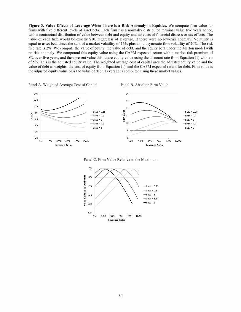
Figure 3 shows the cost of capital and firm value as a function of leverage for a variety of

asset risk levels. In the absence of a risk anomaly, cash flows both grow and are discounted at the

CAPM rate, so firm value is the same at all asset risk levels. In the Figure we modify the value of

equity using the risk anomaly in Equation (1) with an anomaly of 𝛾 = 5% per year, which is

roughly the value we estimate.

19

The figure shows how an equity beta greater than one makes use of the anomaly and

raises value. An equity beta less than one reduces value, and then some, in passing it up. Because

the only effects here are through the weighted average cost of capital, with no cash flow effects,

a weighted average cost of capital minimum in Panel A is equivalent to a firm value maximum in

Panel B. Finally, under a risk anomaly, high asset risk means higher valuations at any level of

leverage, Panel C removes this effect and shows value levels relative to the maximum for each

level of asset risk. This panel shows that at least under these calibration parameters, failing to

exploit the risk anomaly can lead to large losses in firm value.

C. Predictions

These figures illustrate the effects of a risk anomaly on capital structure choice and the

main testable prediction: All else equal, leverage should be set inversely to asset beta.

We restate the mechanism here. It is easiest to see in terms of extreme cases. First, low

leverage firms that start with a high asset beta have only modest incentives to issue debt. Their

high-risk equity is already highly valued. Although there may be a small additional amount of

value to a bit of debt (the value maximum is not quite at zero leverage), even a small exogenous

cost of accessing the debt markets could lead a firm to zero debt. Or, if managers of unlevered

firms follow a simpler rule of thumb, executing a leveraged recapitalization (substituting equity

for debt) only when equity is undervalued by the CAPM, they may also choose zero debt.

This may help to explain a portion of the low leverage puzzle broached by Miller (1977)

and clearly documented by Graham (2000). As an example, Linear Technology Corporation

(Nasdaq: LLTC) produces semiconductors with a market capitalization of $7.7 billion as of

December 2012. Despite profitable operations, a pre-interest marginal tax rate of 35% by the

20

methodology in Graham and Mills (2008), and a cash balance of $1 billion, Linear maintains

negative net debt. One explanation for this may be its high asset beta.

While rarer than inexplicably low-leverage firms, a number of profitable firms maintain

high leverage despite little tax benefit, tempting a fate of financial distress. An example is

Textainer (NYSE: TGH), a firm that leases and trades marine cargo containers. As of the end of

2012, its market capitalization was approximately $1.7 billion. It has tangible assets of $3.4

billion and a cash balance of $175 million. Despite a marginal tax rate close to 0%, as a result of

front-loaded depreciation, modest growth, and an offshore tax status, it maintains $2.7 billion in

debt. A potential explanation for this failure of the standard tradeoff theory is the firm’s low

asset beta. Equity is undervalued at low leverage, and its value rises steadily as leverage

increases to its correct valuation, and potentially beyond.

The risk anomaly tradeoff is also pertinent to a set of uniquely highly leveraged firms—

banks—which are often excluded from capital structure analyses. As Figure 3 shows, a risk

anomaly in equities means that regulating low asset beta firms, in the sense of requiring them to

delever significantly, can impose large losses in private value and increases in the cost of capital.

As an example, Baker and Wurgler (2015) find that banks’ asset betas are on the order of 0.10,

and that the risk anomaly within banks is at least as large as what we find for all firms. While

there are numerous other forces at play in regulatory debates, the loss of the risk anomaly’s

benefits provides one foundation for bankers’ common argument that reducing leverage would

increase their cost of capital (e.g., Elliott (2013)).

Although firms at the leverage extremes are not uncommon, and are particularly

interesting here because they are where the standard tradeoff theory is least compelling, most

21

firms fall in between the extremes. Our regressions explore the extent to which the risk anomaly

tradeoff, as captured through asset beta, can explain the middle of the cross-section as well.

IV. Empirical Tests

A. Data

Our main variables are introduced in Table 5. Our basic sample is the portion of the

merged CRSP-Compustat sample for which marginal tax rates are available from John Graham.

The data begin in 1980, when marginal tax rates are first available, and end in 2012. They

contain 944,099 firm-months and span all 50 Fama-French (1995) industries. Unlike much

capital structure research, we include financial firms because they can be incorporated in the risk

anomaly theory (e.g., Baker and Wurgler (2015)), but their exclusion does not affect the relevant

results. In an average cross-section there are 2,120 profitable and 265 unprofitable firms.

Variable definitions are detailed in Appendix 2. Gross book leverage is long-term debt

and notes payable divided by the sum of long-term debt and notes payable plus book equity. Net

book leverage nets out cash and equivalents from the numerator and denominator. Gross and net

market leverage replace book equity with the market value of common equity from CRSP.

The regressions control for traditional explanatory variables in Bradley, Jarrell, and Kim

(1984), Rajan and Zingales (1995), Baker and Wurgler (2002), Frank and Goyal (2009), and

others. The fixed assets ratio, a proxy for financial distress costs, is net property, plant and

equipment divided by total assets. Profitability, which would be positively correlated with

leverage under the standard tradeoff theory but inversely correlated under the Myers and Majluf

(1984) pecking order, is EBIT divided by total assets. Market-to-book assets is known to be

negatively related to leverage, consistent with the need for firms with strong growth

22

opportunities to avoid having to pass them up (Myers (1977)) or the outcome of equity market

timing (Baker and Wurgler (2002)). It is gross debt and market equity divided by the sum of

gross debt and book equity. Asset growth is more exploratory. It could be a proxy for growth

opportunities, or it could capture size or the profitability that helps to make debt-financed

acquisitions. Firm size, measured as the natural log of book assets, may also proxy for a variety

of influences. Fama and French (1992) use it to represent the greater cash flow volatility of

smaller firms and their higher expected costs of financial distress. It will also be correlated with

their generally lesser access to debt markets. Finally, John Graham’s pre-interest marginal tax

rates account for many features of the tax code. As shown by Graham and Mills (2008), they

approximate the tax rates simulated with federal tax return data.

The leverage determinants that interest us most are constructed from stock returns. Asset

beta is unlevered equity beta, assuming debt is riskless. As we reported earlier, betas on

corporate debt are very low, and in any case it is hard to do better without debt returns data.

Total equity risk is the standard deviation of excess stock returns. Asset risk is the unlevered

version. Industry asset beta and risk are market equity weighted averages.

B. Summary Statistics and Correlations

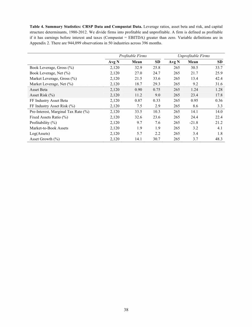
Tables 4 and 5 show summary statistics and correlations. Summary statistics on the

standard capital structure determinants contain no surprises. Profitable firms are larger and have

higher tax rates. Asset beta is somewhat higher for unprofitable firms, at least for own (firm-

specific) asset beta. Total risk is as well. With respect to asset risk, a firm must be promising and

at least on a path to profitability to enter the CRSP-Compustat sample for the 24 months that we

require to compute beta. Becoming unprofitable may be associated with unexpectedly negative

23

returns; also, firms in variable industries are more likely to find themselves unprofitable in a

given period. The latter logic also applies to beta, on the downside.

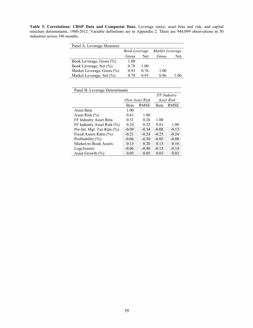
The correlations in Table 5 contain a few insights, however. One is that gross and net

leverage measures are loosely correlated enough to consider both as a robustness exercise. It is

less important to consider both book and market leverage measures, given their 0.93 correlation,

but we follow tradition and do so. The more interesting correlations are those between our risk

measures and standard regression variables. In particular, asset beta risk is negatively correlated

with tax rates, fixed assets, profitability, and size, and positively correlated with market-to-book

and asset growth. Correlations are not transitive, but we will see, and prior research confirms,

that several of these variables then have the opposite sign coefficients in leverage regressions.

We will then need to ask whether the standard variables affect leverage because of an assortment

of different theories, or because they are also picking up on a single force, asset beta risk. We

return to this when we discuss the regressions.

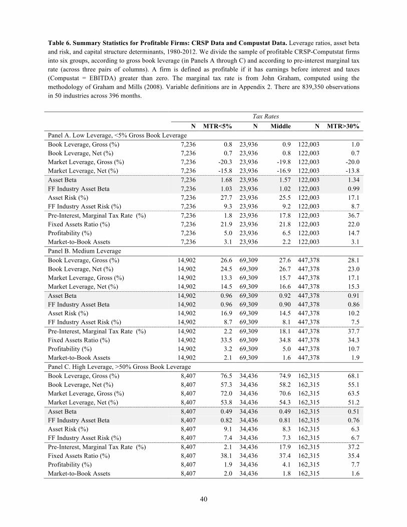
Table 6 looks more closely within profitable firms, where we have 839,350 observations

and where the shortcomings of the standard tradeoff theory appear most clearly. The panels

separate profitable firms into low leverage (gross book leverage <5%), medium leverage, and

high leverage (gross book leverage >50%) groups. Zero leverage is obviously low, but what

counts as high leverage is subjective. We obviously cannot expect a mode at 100%, which is

insolvency, so we choose a cutoff of 50% for simplicity. The columns then add an additional sort

into low (MTR<5%), medium, and high (MTR>30%) marginal tax rate groups.

The low leverage puzzle is represented in the large number of firm-months with positive

profitability, high marginal tax rates, and very low leverage. In fact, these make up 80% of all

profitable, low leverage firms (=122,003/(7,236+23,936+122,003)). Firms like Linear

24

Technology are in this bin. Conversely, there are a number of firm-months where, despite almost

no tax benefit, leverage exceeds 50%. These make up somewhat over 4% of all profitable high-

leverage firms (=8,407/(8,407+34,436+162,315)) and include firms like Textainer.

Some initial support for the risk anomaly tradeoff comes from the strong differences in

asset risk across the leverage levels, which is also essentially independent of tax rates. Within the

middle tax rate group, for example, asset betas decline sharply with leverage. Firms with very

low leverage have a median asset beta of 1.57. This falls to 0.92 for medium leverage firms and

to 0.49 for high leverage firms. Also consistent with the risk anomaly tradeoff is the steady

decline in asset risk. This, however, is somewhat less specific to the theory, as it could in

principle just be another control for financial distress costs. We will, therefore, be more

interested in the effect of asset beta controlling for total asset risk (also like Schwert and

Strebulaev (2014)) in regressions.

C. Regressions: Without Asset Risk

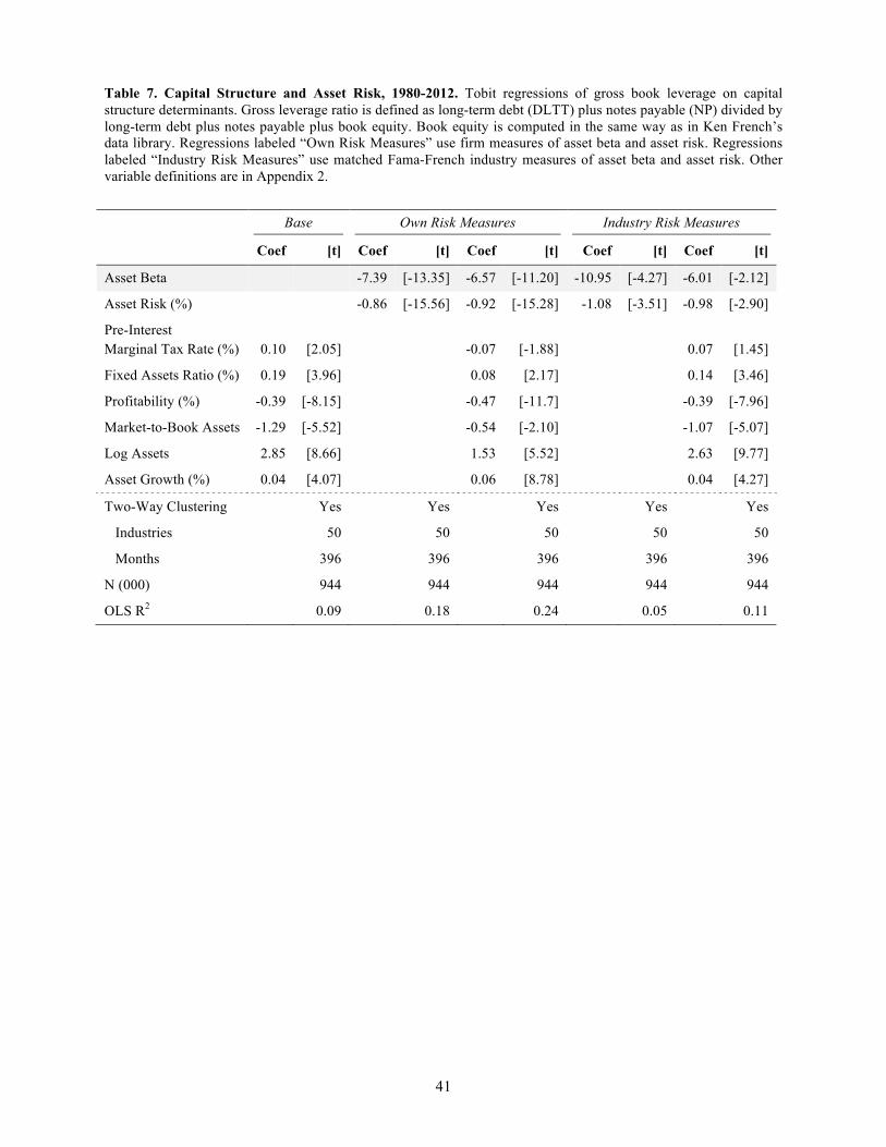
The first column of Table 7 shows a baseline capital structure regression. We report

marginal effects of Tobit regressions that cluster on both firm and month to improve standard

errors. We choose gross book leverage for this baseline and include the typical empirical

covariates. The first several variables’ signs and effects are consistent with prior research, as is

the poor overall R2. The marginal tax rate has a positive coefficient, fixed assets a fairly strong

positive coefficient, profitability a negative coefficient, market-to-book a negative coefficient,

and size a positive coefficient. Rajan and Zingales (1995) focus on these four variables and

obtain the same results. Finally, asset growth has a positive coefficient, rather inconsistent with it

proxying for growth opportunities and more so with the interpretation that asset growth is a

25

consequence of the ability and desire to finance with debt, determined by other underlying

sources, as opposed to a determinant of leverage in its own right.

Each of these variables is often given a somewhat different interpretation. One is used to

proxy for one effect, and another for another. Yet comparing the pattern of signs in this

regression with the signs of correlations suggests an intriguing hypothesis: the standard variables

may also be capturing the single force of asset beta. That is, we hypothesize that asset beta is

negatively related to leverage, and each of these variables, with the exceptions of profitability

and asset growth (where the theory is weaker, as well as the correlation with asset beta), has a

regression coefficient that is the opposite sign to its correlation with asset beta. It is always hard

to know exactly what these variables capture, but it is an interesting possibility that a common

mechanism may contribute to their explanatory power.

D. Regressions: Adding Asset Risk

We now add risk measures to the standard regression determinants. Our special focus is

on asset beta, which is what our theory suggests, but we also control for overall risk. In principle,

any effect of total asset risk could reflect the risk anomaly tradeoff—some explanations of the

risk anomaly are specific to beta, others are not. However, although it is not usually included in

leverage regressions, with the recent exception of Schwert and Strebulaev (2014), total asset risk

is also a plausible proxy for the expected costs of financial distress, especially compared to asset

beta. Firms usually care more about going bankrupt at all than about precisely when it happens.

The middle columns of Table 7 show that asset beta is a strong determinant of leverage,

supporting the main prediction. This is true controlling for overall asset risk (as well as in a

univariate regression). Adding the control variables does not significantly affect the coefficient

26

or t-statistic on asset beta. With all controls, a one-unit increase in asset beta reduces leverage by

6.6%. (The economic effect of total asset risk is larger, though its interpretation is cloudy.)

A problem with this exercise is the mechanical negative link between leverage and asset

beta caused by using leverage itself to unlever the equity beta. One solution is to overcorrect and

use unlevered equity beta and equity volatility. This creates a potential reverse causality that

goes in the opposite direction from the predicted direction. Leverage, if chosen randomly, should

be associated with higher equity betas and volatilities. However, if firms with higher asset risk

choose lower leverage and firms with lower asset risk choose higher leverage in a way that does

not fully equilibrate the betas, as the model predicts, then there will be on net a negative

relationship between beta and leverage. In results available on request, we find that equity beta is

also strongly negatively related to gross and net leverage in both book and market terms.

Our preferred solution is to maintain focus on asset risk but eliminate any mechanical

link by switching to industry measures. Although this likely introduces some measurement error,

the last columns of Table 7 show that the economic effects remain robust to using industry risk.

As a further robustness check, we consider alternative leverage measures in Table 8 that

net out cash, substitute book value with market value equity, or both. We continue to use

industry risk measures here. We find that the effects of asset beta on these leverage measures are

as large or larger as the baseline gross book leverage specification.

E. An Alternative Explanation

It is clear that high asset beta is associated with lower leverage. This is consistent with

the risk anomaly tradeoff whereby the cost of equity for high beta assets is lower and so less debt

is optimal. The fact is also consistent with versions of the standard tradeoff theory, however. The

costs of financial distress depend not only on the unconditional probability of default and value

27

lost in default but also when distress occurs and value is lost. If asset beta, holding all else

constant, including total risk, dictates the market state when distress is likely to occur, then the

present value of the costs of financial distress are higher for assets with higher systematic risk. In

the lingo of asset pricing, it is the covariance of the stochastic discount factor with the costs of

financial distress that determine the present value of distress costs.

Almeida and Philippon (2007) argue that risk-adjustment increases the cost of financial

distress. Shleifer and Vishny (1992) offer the tangible example of refinancing risk and fire sales.

If refinancing risks and fire sale discounts are higher during market downturns, this would

increase the value lost in distress and lower optimal leverage for firms with higher levels of

systematic risk (though it is still hard to justify zero debt in the presence of large tax benefits).

To distinguish further, we make use of a key difference between how risk matters in the

traditional tradeoff and how it matters the risk anomaly tradeoff. In the traditional tradeoff,

“downside risk” is the emphasis; risk matters because of bankruptcy costs. The risk anomaly

model makes no such distinction. Hence, if a beta risk version of the traditional model drives the

link between high asset beta and leverage, it should appear with more strength in downside risk.

This is not the case. We estimate equity beta separately over months when the market risk

premium was positive and when it was negative. Unlevering these and averaging by industry

gives us an upside asset beta and downside asset beta measure. Table 9 shows that if anything, it

is the upside component of asset beta that is inversely related to leverage. The downside

component has no statistical association with leverage and a point estimate of the wrong sign to

support a systematic risk version of the traditional tradeoff theory.

In addition to an empirical advantage, the risk anomaly theory also has a conceptual

advantage relating to its empirically grounded foundation. It is hard for the traditional tradeoff

28

theory, combined with rational asset pricing, to fit both the leverage and asset pricing evidence

on the pricing of beta. If beta is truly a measure of risk, then it would help to explain the cross

section of asset returns, which it does not. Investors, recognizing the investment opportunities,

would demand higher returns on assets exposed to periods of fire sales. If beta is not truly a

measure of risk—as the literature that follows Fama and French (1992, 1993) has claimed—then

asset beta should not be a constraint on leverage, after controlling for total asset risk. The risk

anomaly model naturally accommodates both leverage and asset pricing relationships.

V. Conclusion

Since Modigliani and Miller, the academic literatures on asset pricing and corporate

finance have grown separate. In particular, the corporate finance literature has largely taken the

pricing of risk as given, because the overall cost of capital, and hence optimal capital structure, is

unaffected under the seemingly plausible assumption that markets for different forms of

securities are integrated.

Meanwhile, evidence in asset pricing indicates that high-risk equities do not earn

commensurately high returns. This paper considers the possibility that this pattern reflects

mispricing, driven by a mixture of behavioral and institutional frictions, and uses it to develop a

tradeoff theory of leverage. For firms with relatively risky assets, the cost of capital is minimized

at a low level of leverage. For firms with very low risk assets, low leverage entails a substantial

cost in the form of issuing undervalued equity, and hence the cost of capital is minimized at

much higher levels of leverage. Consistent with a risk anomaly, leverage is inversely related to

systematic risk and may help to resolve both low and high leverage puzzles.

29

References Almeida, Heitor, T. Philippon. “The Risk-Adjusted Cost of Financial Distress.” Journal of Finance 62 (2007), pp. 2557-2586.

Ang, Andrew, R. Hodrick, Y. Xing, X. Zhang. “The Cross-Section of Volatility and Expected Returns.” Journal of Finance 61 (2006), pp. 259-299.

Ang, Andrew, R. Hodrick, Y. Xing, X. Zhang. “High Idiosyncratic Volatility and Low Returns: International and Further U.S. Evidence.” Journal of Financial Economics 91 (2009), pp. 1-23.

Baker, Malcolm, B. Bradley, R. Taliaferro. “The Risk Anomaly: A Decomposition into Micro and Macro Effects.” Harvard Business School, working paper (2013).

Baker, Malcolm, B. Bradley, J. Wurgler. “Benchmarks as Limits to Arbitrage: Understanding the Low-Volatility Anomaly.” Financial Analysts Journal 67 (2011), pp. 40-54.

Baker, Malcolm, J. Wurgler. “Do Strict Capital Requirements Raise the Cost of Capital? Bank Regulation, Capital Structure, and the Risk Anomaly.” American Economic Review 105 (2015), pp. 315-320.

Baker, Malcolm, J. Wurgler. “Comovement and Predictability Relationships Between Bonds and the Cross-Section of Stocks.” Review of Asset Pricing Studies 2 (2012), pp. 57-87.

Bali, Turan, N. Cakici, R. Whitelaw. “Maxing Out: Stocks as Lotteries and the Cross-Section of Expected Returns.” Journal of Financial Economics 99 (2011), pp. 427-446.

Barberis, Nicholas, A. Shleifer. “Style Investing.” Journal of Financial Economics 68 (2003), pp. 161-199.

Barberis, Nicholas, M. Huang. “Stocks as Lotteries: The Implications of Probability Weighting for Security Prices.” American Economic Review 98 (2008), pp. 2066-2100.

Black, Fischer. “Capital Market Equilibrium with Restricted Borrowing.” Journal of Business 45 (1972), pp. 444-455.

Black, Fischer, M. C. Jensen, M. Scholes. “The Capital Asset Pricing Model: Some Empirical Tests.” In M. C. Jensen, ed., Studies in the Theory of Capital Markets. New York: Praeger (1972), pp. 79-121.

Black, Fischer, Myron Scholes, “The Pricing of Options and Corporate Liabilities.” Journal of Political Economy 81 (1973), pp 637-659.

Blitz, David, P. V. Vliet. “The Volatility Effect: Lower Risk Without Lower Return.” Journal of Portfolio Management 34 (2007), pp. 102-113.

30

Blitz, David, J. Pang, P. V. Vliet. “The Volatility Effect in Emerging Markets.” Emerging Markets Review 16 (2013), pp. 31-45.

Bradley, Michael, G. Jarrell, E. H. Kim. “On the Existence of an Optimal Capital Structure: Theory and Evidence.” Journal of Finance 39 (1984), pp. 857-878.

Brennan, Michael. “Agency and Asset Pricing.” University of California, Los Angeles, working paper (1993).

Cornell, Bradford. “The Pricing of Volatility and Skewness: A New Interpretation.” California Institute of Technology working paper (2008).

Elliott, Douglas J. “Higher Bank Capital Requirements Would Come at a Price.” Brookings Institute Internet posting. http://www.brookings.edu/research/papers/2013/02/20-bank-capital-requirements-elliott (February 20, 2013).

Falkenstein, Eric. Mutual Funds, Idiosyncratic Variance, and Asset Returns. PhD thesis (1994), Northwestern University.

Fama, Eugene, K. R. French. “The Cross-Section of Expected Stock Returns.” Journal of Finance 47 (1992), pp. 427-465.

Fama, Eugene, K. R. French. “Common Risk Factors in the Returns on Stocks and Bonds.” Journal of Financial Economics 33 (1993), pp. 3-56.

Fama, Eugene, K. R. French. “Testing Trade-Off and Pecking Order Predictions About Dividends and Debt.” Review of Financial Studies 15 (2002), pp. 1-33.

Frank, Murray Z., V. K. Goyal, “Capital Structure Decisions: Which Factors Are Reliably Important?” Financial Management 38 (2009), pp. 1-37.

Frazzini, Andrea, L. H. Pedersen. “Betting Against Beta.” Journal of Financial Economics 111 (2014), pp. 1-25.

Gibbons, Michael R., S. A. Ross, J. Shanken. “A Test of the Efficiency of a Given Portfolio.” Econometrica 57 (1989), pp. 1121-1152.

Gornall, Will, I. A. Strebulaev. “Financing as a Supply Chain: The Capital Structure of Banks and Borrowers.” Stanford Graduate School of Business working paper (2014).

Graham, John, “How Big Are the Tax Benefits of Debt.” Journal of Finance 63 (2000), pp. 1901-1941.

Graham, John, and L. Mills. “Simulating Marginal Tax Rates Using Tax Return Data.” Journal of Accounting and Economics 46 (2008), pp. 366-388.

31

Harris, Milton, and A. Raviv. “The Theory of Capital Structure.” Journal of Finance 46 (1991), pp. 297-355.

Haugen, Robert A., A. J. Heins, “Risk and the Rate of Return on Financial Assets: Some Old Wine in New Bottles.” Journal of Financial and Quantitative Analysis 10 (1975), pp. 775-784.

Hong, Harrison, D. Sraer. “Speculative Betas.” Princeton University working paper (2012).

Ibbotson Associates, 2012, Ibbotson SBBI 2012 Classic Yearbook (Morningstar, Chicago).

Karceski, Jason. “Returns-Chasing Behavior, Mutual Funds, and Beta’s Death. “ Journal of Financial and Quantitative Analysis 37 (2002), pp. 559-594.

Kumar, Alok. “Who Gambles in the Stock Market?” Journal of Finance 64 (2009), pp. 1889-1933.

Merton, Robert C. “On the Pricing of Corporate Debt: The Risk Structure of Interest Rates.” Journal of Finance 29 (1974), pp. 449–470.

Miller, Merton H., “Debt and Taxes.” Journal of Finance 32, pp. 261-275.

Myers, Stewart, N. Majluf. “Corporate Financing and Investment Decisions When Firms Have Information That Investors Do Not Have.” Journal of Financial Economics 13 (1984), pp. 187-221. Myers, Stewart. “Determinants of Corporate Borrowing.” Journal of Financial Economics 5 (1977), pp. 147-175. Rajan, Raghuram, and L. Zingales. “What Do We Know about Capital Structure? Some Evidence from International Data.” Journal of Finance 50 (1995), pp. 1421-1460. Schwert, Michael, I. A. Strebulaev. “Capital Structure and Systematic Risk.” Stanford University working paper (2014). Shleifer, Andrei, and R. Vishny. “Liquidation Values and Debt Capacity: A Market Equilibrium Approach.” Journal of Finance 47 (1992), pp. 1343-1366. Stein, Jeremy, “Rational Capital Budgeting in an Irrational World.” Journal of Business 69 (1996), pp 429-455.

32

Figure 1. Segmented Debt and Equity Markets. For the risk anomaly to impact the weighted average cost of capital, debt and equity markets must be segmented. Panel A shows a risk anomaly that extends across asset classes, e.g. from safe debt with very low beta to equity with higher beta, rendering capital structure irrelevant. Panels B and C show segmented debt and equity markets, first with debt correctly priced and then with a small risk anomaly.

Panel A. Integrated Debt and Equity Markets Panel B. Markets Not Integrated, Debt Correctly Priced

Panel C. Markets Not Integrated, Small Low Risk Anomaly in Debt Markets

33

Figure 2. Bond Returns and the Risk Anomaly in Stocks. Plots of average returns and CAPM betas for three value weighted equity portfolios sorted into quintiles using pre-ranking betas as well as long-term corporate and government bonds from Ibbotson and Associates. The returns and betas are estimated as in Tables 1 and 2. An empirical security market line is fit through the three equity data points.

Panel A. 1968-2012

Panel B. 1931-2012

34

Figure 3. Value Effects of Leverage When There is a Risk Anomaly in Equities. We compute firm value for firms with five different levels of asset beta. Each firm has a normally distributed terminal value five years hence, with a contractual distribution of value between debt and equity and no costs of financial distress or tax effects. The value of each firm would be exactly $10, regardless of leverage, if there were no low-risk anomaly. Volatility is equal to asset beta times the sum of a market volatility of 16% plus an idiosyncratic firm volatility of 20%. The risk free rate is 2%. We compute the value of equity, the value of debt, and the equity beta under the Merton model with no risk anomaly. We compound this equity value using the CAPM expected return with a market risk premium of 8% over five years, and then present value this future equity value using the discount rate from Equation (1) with a γ of 5%. This is the adjusted equity value. The weighted average cost of capital uses the adjusted equity value and the value of debt as weights, the cost of equity from Equation (1), and the CAPM expected return for debt. Firm value is the adjusted equity value plus the value of debt. Leverage is computed using these market values. Panel A. Weighted Average Cost of Capital Panel B. Absolute Firm Value

Panel C. Firm Value Relative to the Maximum

35

Table 1. Realized Returns and Risk: Beta Portfolios, 1968-2012. Regressions of portfolio returns on market excess returns and the Fama-French factors, SMB and HML. Each portfolio total return in excess of the riskless rate is computed using either equal or value weights. The sample is divided within each month into low (bottom 30%), medium (middle 40%), and high (top 30%) portfolios according to pre-ranking beta. Gibbons, Ross, and Shanken (1989) tests are shown for each set of regressions.

Panel A. Equal Weighted Bottom 30% Middle 40% Top 30% Top – Bottom

Basis Points Coef [t] Coef [t] Coef [t] Coef [t] Mean Excess Returns 71.4 [3.99] 80.5 [3.35] 73.7 [2.16] 2.2 [0.11] CAPM Regressions Market 0.69 [25.70] 1.06 [36.65] 1.44 [31.71] 0.74 [24.39] Intercept 41.1 [3.41] 34.3 [2.66] 11.1 [0.55] -30.1 [-2.22] T 540 540 540 540 R-Squared 0.551 0.714 0.651 0.525 GRS Test (p) 9.10 (<0.01) Fama-French 3-Factor Regressions Market 0.66 [33.64] 0.99 [62.11] 1.32 [45.02] 0.66 [25.24] SMB 0.53 [18.62] 0.71 [30.97] 0.99 [23.58] 0.46 [12.46] HML 0.31 [10.22] 0.40 [16.35] 0.32 [7.00] 0.01 [0.15] Intercept 25.4 [2.92] 15.1 [2.16] -3.4 [-0.26] -28.8 [-2.51] T 540 540 540 540 R-Squared 0.778 0.919 0.864 0.674 GRS Test (p) 5.18 (<0.01) Panel B. Value Weighted Bottom 30% Middle 40% Top 30% Top – Bottom

Basis Points Coef [t] Coef [t] Coef [t] Coef [t] Mean Excess Returns 46.2 [2.99] 45.0 [2.26] 38.6 [1.32] -7.5 [-0.37] CAPM Regressions Market 0.71 [42.46] 1.02 [130.49] 1.42 [59.04] 0.72 [21.11] Intercept 15.3 [2.05] 0.4 [0.12] -23.4 [-2.18] -38.7 [-2.56] T 540 540 540 540 R-Squared 0.770 0.969 0.866 0.453 GRS Test (p) 2.76 (0.04) Fama-French 3-Factor Regressions Market 0.70 [40.73] 0.99 [93.84] 1.34 [69.41] 0.64 [20.04] SMB 0.00 [0.19] 0.00 [-0.02] 0.26 [9.46] 0.26 [5.62] HML 0.15 [5.68] 0.10 [6.19] -0.01 [-0.47] -0.16 [-3.35] Intercept 8.5 [1.12] -2.6 [-0.56] -20.1 [-2.36] -28.6 [-2.03] T 540 540 540 540 R-Squared 0.771 0.948 0.920 0.545 GRS Test (p) 2.71 (0.04)

36

Table 2. Realized Returns and Risk: Beta Portfolios, 1931-2012. Regressions of portfolio returns on market excess returns and the Fama-French factors, SMB and HML. Each portfolio total return in excess of the riskless rate is computed using either equal or value weights. The sample is divided within each month into low (bottom 30%), medium (middle 40%), and high (top 30%) portfolios according to pre-ranking beta. Gibbons, Ross, and Shanken (1989) tests are shown for each set of regressions.

Panel A. Equal Weighted Bottom 30% Middle 40% Top 30% Top – Bottom

Basis Points Coef [t] Coef [t] Coef [t] Coef [t] Mean Excess Returns 94.8 [5.86] 113.3 [4.86] 121.9 [3.83] 27.2 [1.50] CAPM Regressions Market 0.82 [51.44] 1.25 [66.71] 1.64 [56.29] 0.83 [38.31] Intercept 42.3 [4.98] 33.1 [3.31] 16.2 [1.04] -26.0 [-2.25] T 984 984 984 984 R-Squared 0.729 0.819 0.763 0.599 GRS Test (p) 13.55 (<0.01) Fama-French 3-Factor Regressions Market 0.68 [57.77] 1.03 [113.58] 1.35 [82.39] 0.66 [36.81] SMB 0.50 [26.16] 0.71 [48.72] 1.06 [40.47] 0.57 [19.52] HML 0.21 [12.47] 0.40 [30.73] 0.53 [22.33] 0.31 [12.06] Intercept 29.3 [4.93] 11.1 [2.44] -14.5 [-1.76] -43.8 [-4.82] T 984 984 984 984 R-Squared 0.869 0.963 0.935 0.756 GRS Test (p) 11.36 (<0.01) Panel B. Value Weighted Bottom 30% Middle 40% Top 30% Top – Bottom

Basis Points Coef [t] Coef [t] Coef [t] Coef [t] Mean Excess Returns 59.7 [4.51] 71.3 [3.79] 76.3 [2.81] 16.6 [0.95] CAPM Regressions Market 0.73 [80.18] 1.10 [186.67] 1.53 [97.94] 0.80 [38.31] Intercept 12.9 [2.66] 0.8 [0.25] -21.9 [-2.62] -34.8 [-3.12] T 984 984 984 984 R-Squared 0.868 0.973 0.907 0.599 GRS Test (p) 4.22 (<0.01) Fama-French 3-Factor Regressions Market 0.72 [72.45] 1.05 [149.40] 1.42 [105.24] 0.71 [34.80] SMB -0.05 [-2.89] 0.02 [1.37] 0.29 [13.51] 0.34 [10.38] HML 0.05 [3.83] 0.12 [11.59] 0.21 [10.60] 0.15 [5.19] Intercept 11.8 [2.37] -3.0 [-0.84] -32.4 [-4.75] -44.1 [-4.31] T 984 984 984 984 R-Squared 0.863 0.966 0.939 0.668 GRS Test (p) 8.25 (<0.01)

37

Table 3. Debt and Equity Market Segmentation. Regressions of portfolio returns on market excess returns and government bond excess returns. Each portfolio total return in excess of the riskless rate is computed using value weights. The sample is divided within each month into low (bottom 30%), medium (middle 40%), and high (top 30%) portfolios according to pre-ranking beta, using all CRSP stocks. We also compute the returns to corporate bonds in excess of the riskless rate using data from Ibbotson and Associates. Below we show the market beta, government bond beta, and the alpha (or intercept) for the Bottom 30% portfolio in absolute terms and for the Top 30% portfolio and corporate bonds in relation to the Bottom 30%. The final column compares the extrapolated alpha using the relationship between alpha and beta in the Bottom and Top 30% portfolios to the actual alpha for corporate bonds. In an integrated market, where the low beta anomaly holds equally in stock and bond markets, the actual and extrapolated betas are the same. There are 540 months in the first two panels and 984 in the second two panels.

Bottom 30% Top - Bottom 30% Corporate – Bottom 30%

Extrapolated Corporate – Bottom 30%

Basis Points Coef [t] Coef [t] Coef [t] Coef [prob] CAPM Regressions, January 1968-December 2012 Market 0.67 [36.32] 0.72 [27.57] -0.51 [-19.56] Intercept 17.0 [1.97] -38.8 [-3.18] 5.1 [0.42] 27.6 Difference -22.4 [p =0.104] R-Squared 0.8198 CAPM Regressions with Government Bond Returns, January 1968-December 2012 Market 0.66 [44.54] 0.75 [36.04] -0.57 [-27.24] Bonds 0.16 [7.42] -0.32 [-10.29] 0.60 [19.27] Intercept 12.9 [1.89] -30.9 [-3.19] -9.8 [-1.01] 23.3 Difference -33.1 [p =0.014] R-Squared 0.888 CAPM Regressions, January 1931-December 2012 Market 0.71 [63.79] 0.80 [50.64] -0.63 [-39.63] Intercept 13.6 [2.24] -35.1 [-4.09] 3.8 [0.45] 27.5 Difference -23.6 [p =0.036] R-Squared 0.8899 CAPM Regressions with Government Bond Returns, January 1931-December 2012 Market 0.71 [72.54] 0.82 [59.57] -0.66 [-47.66] Bonds 0.17 [8.01] -0.36 [-11.86] 0.57 [18.83] Intercept 10.7 [2.03] -28.9 [-3.89] -6.0 [-0.80] 23.1 Difference -29.1 [p =0.006] R-Squared 0.9179

38

Table 4. Summary Statistics: CRSP Data and Compustat Data. Leverage ratios, asset beta and risk, and capital structure determinants, 1980-2012. We divide firms into profitable and unprofitable. A firm is defined as profitable if it has earnings before interest and taxes (Compustat = EBITDA) greater than zero. Variable definitions are in Appendix 2. There are 944,099 observations in 50 industries across 396 months.

Profitable Firms Unprofitable Firms Avg N Mean SD Avg N Mean SD

Book Leverage, Gross (%) 2,120 32.9 25.8 265 30.5 33.7 Book Leverage, Net (%) 2,120 27.0 24.7 265 21.7 25.9 Market Leverage, Gross (%) 2,120 21.5 33.6 265 13.4 42.4 Market Leverage, Net (%) 2,120 18.7 29.3 265 9.2 31.6 Asset Beta 2,120 0.90 0.75 265 1.24 1.28 Asset Risk (%) 2,120 11.2 9.0 265 23.4 17.8 FF Industry Asset Beta 2,120 0.87 0.33 265 0.95 0.36 FF Industry Asset Risk (%) 2,120 7.5 2.9 265 8.6 3.3 Pre-Interest, Marginal Tax Rate (%) 2,120 33.5 10.3 265 14.1 14.0 Fixed Assets Ratio (%) 2,120 32.6 23.6 265 24.4 22.4 Profitability (%) 2,120 9.7 7.6 265 -21.8 21.2 Market-to-Book Assets 2,120 1.9 1.9 265 3.2 4.1 Log(Assets) 2,120 5.7 2.2 265 3.4 1.8 Asset Growth (%) 2,120 14.1 30.7 265 3.7 48.3

39

Table 5. Correlations: CRSP Data and Compustat Data. Leverage ratios, asset beta and risk, and capital structure determinants, 1980-2012. Variable definitions are in Appendix 2. There are 944,099 observations in 50 industries across 396 months.

Panel A. Leverage Measures Book Leverage Market Leverage Gross Net Gross Net Book Leverage, Gross (%) 1.00 Book Leverage, Net (%) 0.78 1.00 Market Leverage, Gross (%) 0.93 0.76 1.00 Market Leverage, Net (%) 0.78 0.93 0.86 1.00

Panel B. Leverage Determinants

Own Asset Risk FF Industry Asset Risk

Beta RMSE Beta RMSE Asset Beta 1.00 Asset Risk (%) 0.61 1.00 FF Industry Asset Beta 0.31 0.26 1.00 FF Industry Asset Risk (%) 0.24 0.32 0.81 1.00 Pre-Int. Mgl. Tax Rate (%) -0.09 -0.34 -0.08 -0.13 Fixed Assets Ratio (%) -0.21 -0.24 -0.25 -0.24 Profitability (%) -0.06 -0.30 -0.05 -0.08 Market-to-Book Assets 0.13 0.20 0.13 0.16 Log(Assets) -0.06 -0.40 -0.15 -0.14 Asset Growth (%) 0.05 0.05 0.03 0.03

40

Table 6. Summary Statistics for Profitable Firms: CRSP Data and Compustat Data. Leverage ratios, asset beta and risk, and capital structure determinants, 1980-2012. We divide the sample of profitable CRSP-Computstat firms into six groups, according to gross book leverage (in Panels A through C) and according to pre-interest marginal tax rate (across three pairs of columns). A firm is defined as profitable if it has earnings before interest and taxes (Compustat = EBITDA) greater than zero. The marginal tax rate is from John Graham, computed using the methodology of Graham and Mills (2008). Variable definitions are in Appendix 2. There are 839,350 observations in 50 industries across 396 months. Tax Rates

N MTR<5% N Middle N MTR>30% Panel A. Low Leverage, <5% Gross Book Leverage Book Leverage, Gross (%) 7,236 0.8 23,936 0.9 122,003 1.0 Book Leverage, Net (%) 7,236 0.7 23,936 0.8 122,003 0.7 Market Leverage, Gross (%) 7,236 -20.3 23,936 -19.8 122,003 -20.0 Market Leverage, Net (%) 7,236 -15.8 23,936 -16.9 122,003 -13.8 Asset Beta 7,236 1.68 23,936 1.57 122,003 1.34 FF Industry Asset Beta 7,236 1.03 23,936 1.02 122,003 0.99 Asset Risk (%) 7,236 27.7 23,936 25.5 122,003 17.1 FF Industry Asset Risk (%) 7,236 9.3 23,936 9.2 122,003 8.7 Pre-Interest, Marginal Tax Rate (%) 7,236 1.8 23,936 17.8 122,003 36.7 Fixed Assets Ratio (%) 7,236 21.9 23,936 21.8 122,003 22.0 Profitability (%) 7,236 5.0 23,936 6.5 122,003 14.7 Market-to-Book Assets 7,236 3.1 23,936 2.2 122,003 3.1 Panel B. Medium Leverage Book Leverage, Gross (%) 14,902 26.6 69,309 27.6 447,378 28.1 Book Leverage, Net (%) 14,902 24.5 69,309 26.7 447,378 23.0 Market Leverage, Gross (%) 14,902 13.3 69,309 15.7 447,378 17.1 Market Leverage, Net (%) 14,902 14.5 69,309 16.6 447,378 15.3 Asset Beta 14,902 0.96 69,309 0.92 447,378 0.91 FF Industry Asset Beta 14,902 0.96 69,309 0.90 447,378 0.86 Asset Risk (%) 14,902 16.9 69,309 14.5 447,378 10.2 FF Industry Asset Risk (%) 14,902 8.7 69,309 8.1 447,378 7.5 Pre-Interest, Marginal Tax Rate (%) 14,902 2.2 69,309 18.1 447,378 37.7 Fixed Assets Ratio (%) 14,902 33.5 69,309 34.8 447,378 34.3 Profitability (%) 14,902 3.2 69,309 5.0 447,378 10.7 Market-to-Book Assets 14,902 2.1 69,309 1.6 447,378 1.9 Panel C. High Leverage, >50% Gross Book Leverage Book Leverage, Gross (%) 8,407 76.5 34,436 74.9 162,315 68.1 Book Leverage, Net (%) 8,407 57.3 34,436 58.2 162,315 55.1 Market Leverage, Gross (%) 8,407 72.0 34,436 70.6 162,315 63.5 Market Leverage, Net (%) 8,407 53.8 34,436 54.3 162,315 51.2 Asset Beta 8,407 0.49 34,436 0.49 162,315 0.51 FF Industry Asset Beta 8,407 0.82 34,436 0.81 162,315 0.76 Asset Risk (%) 8,407 9.1 34,436 8.3 162,315 6.3 FF Industry Asset Risk (%) 8,407 7.4 34,436 7.3 162,315 6.7 Pre-Interest, Marginal Tax Rate (%) 8,407 2.1 34,436 17.9 162,315 37.2 Fixed Assets Ratio (%) 8,407 38.1 34,436 37.4 162,315 35.4 Profitability (%) 8,407 1.9 34,436 4.1 162,315 7.7 Market-to-Book Assets 8,407 2.0 34,436 1.8 162,315 1.6

41

Table 7. Capital Structure and Asset Risk, 1980-2012. Tobit regressions of gross book leverage on capital structure determinants. Gross leverage ratio is defined as long-term debt (DLTT) plus notes payable (NP) divided by long-term debt plus notes payable plus book equity. Book equity is computed in the same way as in Ken French’s data library. Regressions labeled “Own Risk Measures” use firm measures of asset beta and asset risk. Regressions labeled “Industry Risk Measures” use matched Fama-French industry measures of asset beta and asset risk. Other variable definitions are in Appendix 2.

Base Own Risk Measures Industry Risk Measures

Coef [t] Coef [t] Coef [t] Coef [t] Coef [t]

Asset Beta -7.39 [-13.35] -6.57 [-11.20] -10.95 [-4.27] -6.01 [-2.12]

Asset Risk (%) -0.86 [-15.56] -0.92 [-15.28] -1.08 [-3.51] -0.98 [-2.90]

Pre-Interest Marginal Tax Rate (%) 0.10 [2.05] -0.07 [-1.88] 0.07 [1.45]

Fixed Assets Ratio (%) 0.19 [3.96] 0.08 [2.17] 0.14 [3.46]

Profitability (%) -0.39 [-8.15] -0.47 [-11.7] -0.39 [-7.96]

Market-to-Book Assets -1.29 [-5.52] -0.54 [-2.10] -1.07 [-5.07]

Log Assets 2.85 [8.66] 1.53 [5.52] 2.63 [9.77]

Asset Growth (%) 0.04 [4.07] 0.06 [8.78] 0.04 [4.27]

Two-Way Clustering Yes Yes Yes Yes Yes

Industries 50 50 50 50 50

Months 396 396 396 396 396

N (000) 944 944 944 944 944

OLS R2 0.09 0.18 0.24 0.05 0.11

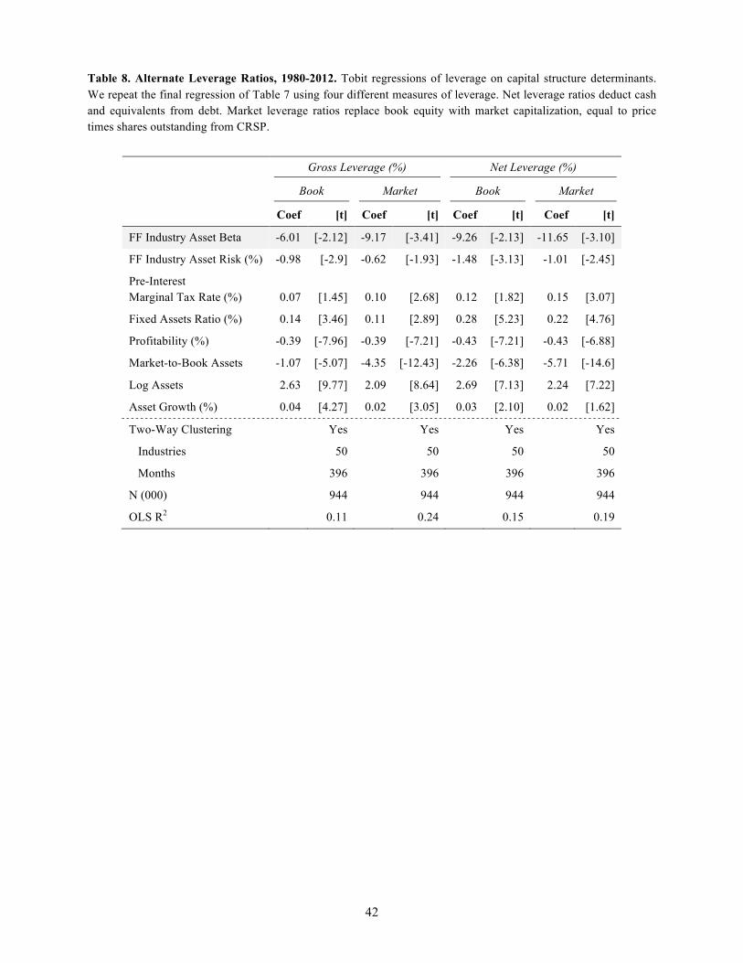
42

Table 8. Alternate Leverage Ratios, 1980-2012. Tobit regressions of leverage on capital structure determinants. We repeat the final regression of Table 7 using four different measures of leverage. Net leverage ratios deduct cash and equivalents from debt. Market leverage ratios replace book equity with market capitalization, equal to price times shares outstanding from CRSP.

Gross Leverage (%) Net Leverage (%)

Book Market Book Market

Coef [t] Coef [t] Coef [t] Coef [t]

FF Industry Asset Beta -6.01 [-2.12] -9.17 [-3.41] -9.26 [-2.13] -11.65 [-3.10]

FF Industry Asset Risk (%) -0.98 [-2.9] -0.62 [-1.93] -1.48 [-3.13] -1.01 [-2.45]

Pre-Interest Marginal Tax Rate (%) 0.07 [1.45] 0.10 [2.68] 0.12 [1.82] 0.15 [3.07]

Fixed Assets Ratio (%) 0.14 [3.46] 0.11 [2.89] 0.28 [5.23] 0.22 [4.76]

Profitability (%) -0.39 [-7.96] -0.39 [-7.21] -0.43 [-7.21] -0.43 [-6.88]

Market-to-Book Assets -1.07 [-5.07] -4.35 [-12.43] -2.26 [-6.38] -5.71 [-14.6]

Log Assets 2.63 [9.77] 2.09 [8.64] 2.69 [7.13] 2.24 [7.22]

Asset Growth (%) 0.04 [4.27] 0.02 [3.05] 0.03 [2.10] 0.02 [1.62]

Two-Way Clustering Yes Yes Yes Yes

Industries 50 50 50 50

Months 396 396 396 396

N (000) 944 944 944 944

OLS R2 0.11 0.24 0.15 0.19

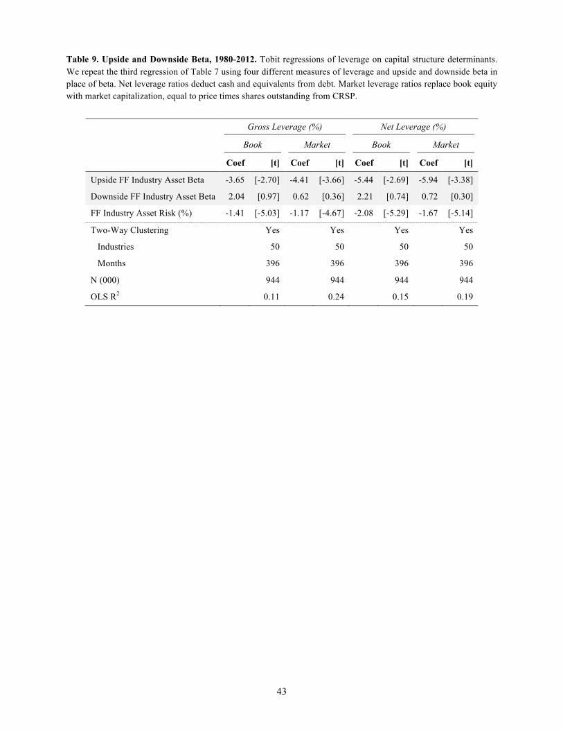
43

Table 9. Upside and Downside Beta, 1980-2012. Tobit regressions of leverage on capital structure determinants. We repeat the third regression of Table 7 using four different measures of leverage and upside and downside beta in place of beta. Net leverage ratios deduct cash and equivalents from debt. Market leverage ratios replace book equity with market capitalization, equal to price times shares outstanding from CRSP.

Gross Leverage (%) Net Leverage (%)

Book Market Book Market

Coef [t] Coef [t] Coef [t] Coef [t]

Upside FF Industry Asset Beta -3.65 [-2.70] -4.41 [-3.66] -5.44 [-2.69] -5.94 [-3.38]

Downside FF Industry Asset Beta 2.04 [0.97] 0.62 [0.36] 2.21 [0.74] 0.72 [0.30]

FF Industry Asset Risk (%) -1.41 [-5.03] -1.17 [-4.67] -2.08 [-5.29] -1.67 [-5.14]

Two-Way Clustering Yes Yes Yes Yes

Industries 50 50 50 50

Months 396 396 396 396

N (000) 944 944 944 944

OLS R2 0.11 0.24 0.15 0.19

44

Appendix 1. Leverage has an Interior Optimum.

We can show more formally that the second-order condition holds. This requires the debt

beta be convex in the equity ratio, or

∂2βd (e,βa,T )∂e(d,T )2

≥ 0 .  

For the following steps, let us consider the debt ratio,  

δ(d,T ) =1− e(d,T ) =1−Φ(x1)+ dΦ(x2 ) , (A1)

which is continuous and strictly increasing in d. Let b be an arbitrary positive number, then from

Theorem 1 in Cargo (1965) it follows that if the debt beta and the debt ratio in Equation (6) and

(A1) are continuous, strictly increasing functions on the interval d ∈ (0,b) , then the debt beta is

convex with respect to the debt ratio if and only if

∂βd (d,βa,T ) /∂d∂δ(d,T ) /∂d

= βa

Φ(x2 )φ(x1)σ τ

+ 1−Φ(x1)[ ]φ(x2 )σ τ

+Φ(x1)Φ(x2 )−Φ(x2 )⎡

⎣⎢⎤

⎦⎥

1−Φ(x1)+ dΦ(x2 )[ ]2 Φ(x2 )−φ(x2 )σ τ

+φ(x1)dσ τ

⎡

⎣⎢⎤

⎦⎥

is non-decreasing on (0,b). That is,

∂2βd (d,βa,T )∂[δ(d,T )]2

≥ 0 .

We can establish that this is convex over all levels of capital, provided that the level of volatility

τσ is not extreme. This establishes that the debt beta is convex in the equity ratio and that

Equation (10) is at least in general positive.

45

Appendix 2. Variable Definitions. All variables are Winsorized at 1% and 99% as measured across the whole sample. Asset Beta Beta times one minus net market leverage. Asset Growth The annual change in total assets (AT) divided by total assets one year ago, in

percentage terms. Asset Risk (%) Risk times one minus market leverage, net. Beta Market beta computed from CRSP returns (RET) net of Treasury bill returns (YLDMAT)

from CRSP regressed on the value-weighted market return (VWRET), also net of the Treasury bill return. We require at least 24 months of returns and use at most 60 months of returns.

Book Equity Shareholder’s equity minus preferred stock plus deferred taxes. Shareholder’s equity (SEQ) or the sum of common equity (CEQ) plus preferred stock (PSTK) if shareholder’s equity is missing or total assets (AT) minus total liabilities (LT) if common equity is missing. Preferred stock is equal to the redemption value of preferred stock (PSTKRV) or the liquidating value of preferred stock (PSTKL) or total preferred stock (PSTK) in that order and set to zero if still missing. Deferred taxes are equal to deferred tax and investment tax credit (TXDITC) or balance sheet deferred tax (TXDB) in that order and zero if missing.

Book Leverage, Gross (%) The sum of total long-term debt (COMPUSTAT = DLTT) and notes payable (NP) divided by the sum of total long-term debt and notes payable and book equity, in percentage terms.

Book Leverage, Net (%) The sum of total long-term debt (COMPUSTAT = DLTT) and notes payable (NP) less cash and equivalents (CHE) divided by the sum of total long-term debt and notes payable and book equity less cash and equivalents, in percentage terms.

FF Industry Asset Beta Market equity weighted average asset beta, computed for each Fama-French industry classification. Market equity is equal to price (PRC) times shares outstanding (CRSP) from CRSP. The 49 industry classifications are defined in Ken French’s data library.

FF Industry Asset Risk (%) Market equity weighted average asset risk, computed for each Fama-French industry classification. Market equity is equal to price (PRC) times shares outstanding (CRSP) from CRSP. The 49 industry classifications are defined in Ken French’s data library.

Fixed Assets Ratio (%) Plant, property, and equipment, net (PPENT) divided by total assets (AT), in percentage terms.

Log Assets The natural log of total assets (AT). Market-to-Book Assets Sum of total long-term debt (COMPUSTAT = DLTT) and notes

payable (NP) and market equity divided by the sum of total long-term debt and notes payable and book equity. Market equity is equal to price (PRC) times shares outstanding (CRSP) from CRSP.

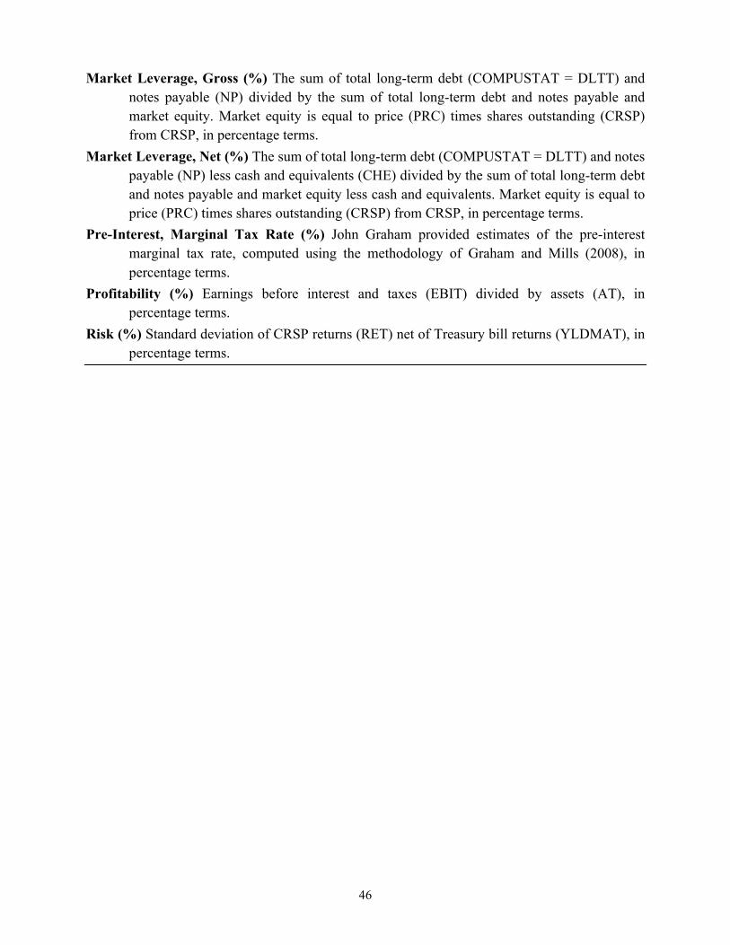
46

Market Leverage, Gross (%) The sum of total long-term debt (COMPUSTAT = DLTT) and notes payable (NP) divided by the sum of total long-term debt and notes payable and market equity. Market equity is equal to price (PRC) times shares outstanding (CRSP) from CRSP, in percentage terms.

Market Leverage, Net (%) The sum of total long-term debt (COMPUSTAT = DLTT) and notes payable (NP) less cash and equivalents (CHE) divided by the sum of total long-term debt and notes payable and market equity less cash and equivalents. Market equity is equal to price (PRC) times shares outstanding (CRSP) from CRSP, in percentage terms.

Pre-Interest, Marginal Tax Rate (%) John Graham provided estimates of the pre-interest marginal tax rate, computed using the methodology of Graham and Mills (2008), in percentage terms.

Profitability (%) Earnings before interest and taxes (EBIT) divided by assets (AT), in percentage terms.

Risk (%) Standard deviation of CRSP returns (RET) net of Treasury bill returns (YLDMAT), in percentage terms.