Embed Size (px)
Citation preview
The riparian vegetation of the Hottentots
Holland Mountains, SW Cape
By
E.J.J. Sieben
Dissertation presented in partial fulfilment of the requirements for the degree of Doctor of Philosophy at the University of Stellenbosch Promoter: Dr. C. Boucher
December 2000

Declaration I the undersigned, hereby declare that the work in this dissertation is my own original work and has not previously, in its entirety or in part, been submitted at any University for a degree. Signature Date
Aan mijn ouders
i
Summary
Riparian vegetation has received a lot of attention in South Africa recently, mainly
because of its importance in bank stabilization and its influence on flood regimes and
water conservation. The upper reaches have thus far received the least of this attention
because of their inaccessibility. This study mainly focuses on these reaches where
riparian vegetation is still mostly in a pristine state. The study area chosen for this
purpose is the Hottentots Holland Mountains in the Southwestern Cape, the area with
the highest rainfall in the Cape Floristic Region, which is very rich in species. Five
rivers originate in this area and the vegetation described around them covers a large
range of habitats, from high to low altitude, with different geological substrates and
different rainfall regimes.
All of these rivers are heavily disturbed in their lower reaches but are still
relatively pristine in their upper reaches. All of them are dammed in at least one place,
except for the Lourens River. An Interbasin Transfer Scheme connects the Eerste-,
Berg- and Riviersonderend Rivers. The water of this scheme is stored mainly in
Theewaterskloof Dam. Another big dam for water storage, Skuifraam Dam, will be
built on the Berg River near Franschhoek in the nearby future.
In order to study the vegetation around a river, a zonation pattern on the river
bank is described and several physical habitats are recognized. A primary distinction
is made between a Wet Bank (flooding at least once a year) and a Dry Bank (flooding
less than once a year). The Dry Bank is further subdivided into a Lower Dynamic, a
Shrub/Tree and a Back Dynamic Zone. In the lower reaches these zones are very
distinct, but in the upper reaches of a river they tend to blend into each other and some
zones can be absent or very narrow.
Vegetation has been sampled in transects across the riverbed, following the
Braun-Blanquet method. Additional vegetation samples have been recorded in the
bogs and mires at the sources of the rivers. Vegetation structure and physical habitat
has been described to contribute to the description of the vegetation types. In order to
understand the environmental processes that determine the vegetation, environmental
parameters were recorded in every vegetation sample, such as, slope, aspect,
rockiness and soil variables.
The classification of the vegetation samples resulted in the identification and
subsequent description of 26 riverine and 11 mire communities. The riverine
ii
communities have been subdivided into ten Community Groups, including a group of
Aquatic communities and three groups of Wet Bank communities. The main
distinction within the Wet Bank Zone is the importance of erosion or deposition as a
driving force of the ecosystem. Three groups of Fynbos communities are identified in
the Back Dynamic Zone, with Asteraceous Fynbos occurring on shales and granites,
Ericaceous Fynbos occurring on Table Mountain Group sandstones and Transitional
Fynbos on a variety of substrates. One community group is characterized by the
dominance of Cliffortia odorata, which shows affinity with some renosterveld
communities known from literature. The two final groups contain the Afromontane
Forests and Riparian Scrub communities, respectively.
Discharges are calculated from data recorded at existing gauging weirs. The
recurrence intervals, inundation levels and stream power of several flood events are
derived from these data and are extrapolated to upstream sites. It appears that most
vegetation types in the zonation pattern on the riverbank can be explained by these
flood events, except for the Afromontane Forests, which are dependent on other site-
specific factors including protection from fire.
Constrained and unconstrained ordinations are used to relate vegetation
patterns to the environment. The vegetation is determined by three environmental
gradients, operating at different scales. The lateral gradient across the riverbed is
mainly determined by inundation frequency and stream power, which are difficult to
measure in rocky mountain situations, although variables like distance from the
water’s edge, elevation above the water level and rockiness are correlated to them.
The longitudinal gradient is the gradient along the length of the river, from high to
low altitude. This gradient has the least influence on the riparian vegetation. The
geographical gradient reflects the large-scale climatic processes across the mountain
range. This gradient accounts for the biggest part of the total explained variation.
Important variables are especially the ratio between the summer and winter rainfall
and the geological substrate. In the Fynbos Biome, where gamma diversity is
extremely high, large-scale environmental processes are important in azonal
vegetation as well. The most species-rich vegetation associated with the rivers is
found furthest from the water’s edge at intermediate altitudes.
Knowledge about the vegetation types and environmental processes in
Western Cape rivers is essential for monitoring and maintaining these special
ecosystems. Specific threats are related to possible abstraction of water from the

iii
Table Mountain Group aquifer and from climate change, which might result in an
overall drying of the ecosystem.
iv
Opsomming
Riviere se oewerplantegroei kry die laaste tyd baie aandag in Suid-Afrika,
hoofsaaklik vanweë die belang vir die beheer van vloede, stabilisasie van die oewers
en die bewaring van drinkwater. Die hoë-liggende dele van die riviere het tot dusver
die minste aandag geniet omdat hulle tot ’n groot mate ontoeganklik is weens die
onherbergsame terrein waarin hulle geleë is. In hierdie studie is daar veral na
bergstrome gekyk waar die plantegroei nog taamlik natuurlik en onversteur is. Die
studiegebied wat vir hierdie doel gekies is, is die Hottentots-Holland berge in die
Wes-Kaap. Die gebied het die hoogste reënval in die Kaapse Floristiese Ryk en is ook
baie ryk aan spesies. Vyf riviere het in hierdie gebied hulle oorsprong. Die plantegroei
wat hier voorkom sluit ‘n wye reeks habitatte in: van hoog tot laag in hoogte bo
seespieël, verskeie geologiese substrate asook verskillende reënval patrone.
Al die vyf riviere wat ondersoek is, is baie versteur in hul onderlope, maar is
nog grotendeels natuurlik in hul hoë-liggende dele. Almal is reeds opgedam deur een
of meer damme, behalwe die Lourensrivier. ’n Tussenopvanggebied-oordragskema
verbind tans die Eerste-, Berg- en Riviersonderendriviere met mekaar. Die water uit
hierdie riviere word tans hoofsaaklik in die Theewaterskloofdam opgegaar. ’n
Verdere groot opgaardam, die sogenaamde Skuifraamdam, word binnekort in die
Bergrivier te Franschhoek gebou.
Al die riviere se onderlope is tot ’n mindere of meerdere mate vervuil met
landbou- en rioolafvoerprodukte. Uitheemse indringerplante, wat die natuurlike
oewerplantegroei verdring, skep veral probleme stroomaf van plantasies en dorpe.
Om die plantegroei van die rivieroewers na te vors, te klassifiseer en te
beskryf, is variasies in die fisiese omgewing bepaal en korrelasies gesoek om die
verspreiding van die plantegroei te verklaar. Die belangrikste verdeling in die
oewerplantegroei wat gevind is, is tussen die Nat-oewersone (dit word meer as een
keer per jaar oorstroom) en die Droë-oewersone (dit word minder as een keer per jaar
oorstroom). Die Droë-oewersone word verder onderverdeel in die Laer-
dinamiesesone, die Boom/Struiksone en die Agter-dinamiesesone. In die laer dele van
die rivier is hierdie soneringspatrone baie duidelik, maar in die boonste dele van die
rivier kan die onderverdelings dikwels nie van mekaar onderskei word nie omdat
hulle gemeng is, of kan die sones baie smal wees of selfs heeltemal afwesig wees.
v
Die plantegroei is gemonster in transekte wat dwarsoor die rivierloop uitgelê
is. Die Braun-Blanquet monstertegniek is gevolg. Bykomende monsterpersele is
opgemeet in die moerasse in die boonste dele van die berg-opvanggebiede. Om die
omgewingsprosesse wat die plantegroei bepaal te verstaan, is ’n aantal
omgewingsfaktore in elke monsterperseel aangeteken, wat, onder andere, helling,
aspek en bedekking van rotse ingesluit het, terwyl die variasie in samestelling van die
bodem ook aangeteken is.
Die klassifikasie van die plantegroei het tot die beskrywing van 26
plantgemeenskappe in die riviere en 11 gemeenskappe in die moerasse gelei. Die
struktuur van die plantegroei asook kenmerke van die fisiese habitat is in die
beskrywing van die plantegroei-eenhede ingesluit. Die gemeenskappe in die riviere is
onderverdeel in tien gemeenskapsgroepe. Daar is een gemeenskapsgroep wat die
akwatiese gemeenskappe en drie wat die Nat-oewersone gemeenskappe insluit. Die
belangrikste verskille tussen die verskillende Nat-oewersone gemeenskappe word
bepaal deur die mate waartoe erosie of deposisie voorkom. Daar is ook drie
gemeenskapsgroepe van Fynbos onderskei wat in die Agter-dinamiesesone voorkom.
Dit sluit in die Aster-fynbos op die skalies en graniete, die Erica-fynbos op die
sandstene en die Oorgangs-fynbos op gemengde substrate. Een gemeenskapsgroep is
deur die dominansie van Cliffortia odorata gekenmerk. Dit toon verwantskap met
renosterveld gemeenskappe wat reeds in die literatuur beskryf is. Die laaste twee
groepe sluit die Afromontane woude en Oewerstruikbosse in.
Die waterafloop is bereken deur middel van data verkry vanaf bestaande
keerwal meetstasies. Die herhalings-intervalle, oorstromingsdiepte en vloei-sterkte
van verskillende vloedtipes word vanaf hierdie data afgelei en stroomop
geekstrapoleer. Die meeste plantegroeivariasie op die oewers kan deur die vloede
verklaar word, behalwe in die geval van die Afromontane woude, wat deur ander
omgewingsfaktore bepaal is.
Beperkte en onbeperkte ordinasie is gebruik om die verband tussen die
plantegroeipatrone en die omgewing te bepaal. Die plantegroei se verspreiding is
bepaal deur drie omgewingsgradiënte, wat op verskillende skale ‘n uitwerking het.
Die laterale gradiënt oor die rivierbedding is hoofsaaklik bepaal deur
oorstromingsfrekwensie en stroomvloeisterkte. Hierdie veranderlikes is moeilik
bepaalbaar, alhoewel ander soos, afstand vanaf die rivier, hoogte bo watervlak en
bedekking van rotse, wat hieraan gekorreleer is, wel meetbaar is. Die lengte gradiënt,
vi
dit is die gradiënt wat van oorsprong na einde langs die lengte van die rivier
teenwoordig is, het die minste invloed op die plantegroei. Die geografiese gradiënt
weerspieel die grootskaalse klimaatsveranderinge oor die bergreeks. Deur hierdie
gradiënt word die grootste deel van die totale variasie tussen die monsters verklaar.
Die belangrikste veranderlikes is die verhouding van somer- teenoor winter-reënval
en die geologiese substraat.
Soortgelyk aan die fynbos in die Fynbosbioom, waar gammadiversiteit
buitegewoon hoog is, is die grootskaalse omgewingsprosesse, ook vir asonale
oewerplantegroei, baie belangrik. Die spesierykste plantegroei rondom die rivier word
die verste van die oewer op gemiddelde hoogtes bo seespieël gevind.
Kennis oor die plantegroei en die omgewingsprosesse in die riviere in die
Wes-Kaap is belangrik vir die monitering en effektiewe beheer van hierdie besondere
ekosisteem. Spesifieke bedreigings is gekoppel aan die potensiële ontginning van
water uit die akwifer in die Tafelberggroep-sedimente asook deur grootskaalse
klimaatsveranderinge waartydens die hoeveelheid water, volgens voorspellings,
waarskynlik sal afneem in hierdie ekosisteem.
vii
Acknowledgements
This thesis would not have been possible without the kind co-operation of many
people from many disciplines and institutions to whom I wish to express my gratitude.
I would like to thank my promotor Dr. C. Boucher for his guidance with this study
and for the opportunity that he gave to me when I came to South Africa for the first
time as a young and curious European scientist who wished to know more about this
magnificent Fynbos Biome. Ms. E. Rode gave me all sorts of assistance, mainly with
computer programs, like Turboveg, Megatab, Canoco and many others. She was
always helpful and I realize that I sometimes gave her a hard time, but she was a great
person to work with.
The staff of the National Botanical Garden’s Compton Herbarium (J. Beyers, D.
Snijman, E.G.H. Oliver, I. Oliver, C. Cupido, J. Manning, J.P. Rourke and J.P. Roux)
helped me with most of my identifications. Taxonomists and ecologists often have a
completely different way of collecting plants and I would never have been able to
achieve quality without their willingness to deal with even the most difficult
identification jobs of ‘scrap material’. The identification of mosses was done by N.
van Rooyen from Pretoria and R. Ochyra from Warsaw.
I am thankful to the staff of the Cape Nature Conservation Board at Jonkershoek and
Nuweberg for access to their beautiful Nature Reserve and the asistance in the field
that I got from them. The officials of SAFCOL also gave me permission to travel
through their plantations in order to get to the Nature Reserve.
Mr. S. Moodley from the Computing Centre of Water Research (CCWR) and Mrs. F.
Sibanyona from the Department of Water Affairs and Forestry (DWAF) kindly put
valuable climatic and hydrological data at my disposal. Dr. H. de Klerk of the Cape
Nature Conservation Board, Scientific Services, also gave me valuable data about the
study area. Dr. R.S. Knight (Department of Biological Sciences, University of the
Western Cape) and Mr. A. van Niekerk (Department of Geography and
Environmental Science, University of Stellenbosch) assisted me with the handling of
viii
the Geographical Information Systems and Mr. M.W. Gordon (Department of Soil
and Irrigation Science, University of Stellenbosch) and Mr. B.H.A. Schloms
(Department of Geography and Environmental Science, University of Stellenbosch)
helped me a great deal with the analysis of the soils.
Prof. A. Görgens, Prof. A. Rooseboom, Prof. G.R. Basson and Mr. J.J. Malan
(Department of Engineering Science, University of Stellenbosch) introduced me to
the scientific fields of hydraulics and hydrology, a discipline that I did not know
anything about before I started this project and really, it is much more interesting than
I ever would have expected. Their valuable discussions and their openness to hear
about my ‘botanical views’ were a great learning experience. Prof. Basson and Mr.
Malan also contributed to the paper that makes up chapter 7 by giving information
about the formulas to use and making a check on my calculations.
I have had valuable discussions about various topics with Prof. V.R. Smith
(Department of Botany, University of Stellenbosch), Prof. S.J. Milton (Dept. of
Nature Conservation and Forestry, University of Stellenbosch), Dr. D. Magadlela
(Working for Water), Mr. A. Chapman (CSIR Stellenbosch), Dr. D.C. le Maitre
(CSIR Stellenbosch), Mr. Barrie Low (Coastec) and Dr. J.M. King (Freshwater
Research Unit, University of Cape Town).
I would like to thank the VSB Fund, the Hugo de Vries Fund, the Backon Foundation
and the National Research Foundation for funding this research project. The Water
Research Commission (Project K5/576, awarded to Dr. J.M. King of the Freshwater
Research Unit, University of Cape Town) sponsored the hydrological research of
which Chapter 7 is the result. The Mazda Wildlife Fund supplied a vehicle for my
use.
There have been many people who joined me in the field and underwent all the
hardships of the fynbos with me. It would be impossible to mention all of those
people here, because many of them were international students of whom I lost track.
Most notable among these was however my visiting father, who climbed down with
me to the Riviersonderend Gorge from Landdroskop and felt completely young again.

ix
At last, I want to express my strong appreciation for the warm friendship and the
moral support that I received from my friends Scotney Watts, Karin Kleinbooi and
Lerato Tsosane. They introduced me to this vast continent, that was like a different
world to me, and the many discussions that we have had about the correlation
between nature conservation, society and poverty alleviation have found their
expression in the last chapter of this thesis.
Erwin Sieben, March 2003.
x
Contents
Summary i
Opsomming iv
Acknowledgements vii
1 General introduction 1
1.1 Focus on riparian vegetation 4 1.2 Aims of this study 5
2 Description of the study area 7
2.1 Choice of the study area 7 2.2 Climate 10
2.2.1 Temperature 13 2.2.2 Solar radiation 14 2.2.3 Precipitation and evaporation 14 2.2.4 Wind 20
2.3 Geology and geomorphology 21 2.3.1 Geology 23 2.3.2 Geomorphology 26
2.4 Soils and pedogenesis 28 2.5 Archaeological to recent history 32
2.5.1 The San and Khoikhoi 32 2.5.2 Early settlers 33 2.5.3 Land use 34
2.6 Botanical background 34 2.6.1 Origins of the Cape Flora 35 2.6.2 Vegetation types in the Fynbos Biome 36 2.6.3 Species diversity 38 2.6.4 Management 40 2.6.5 Earlier studies in the Fynbos Biome 41
2.7 Riverine ecosystems 44 2.7.1 General river ecology 45
2.7.1.1 Mountain streams 46 2.7.1.2 Lower rivers 48 2.7.1.3 Estuaries 49
2.7.2 The river catchment 49 2.7.3 River health 51
2.7.3.1 Water quality 52 2.7.3.2 The flood regime 52 2.7.3.3 The riverbank 54 2.7.3.4 Anthropogenic influences 59
2.7.4 Rivers in the study area 61 2.7.4.1 Eerste River 62 2.7.4.2 Berg River 64 2.7.4.3 Riviersonderend River 67 2.7.4.4 Palmiet River 70 2.7.4.5 Lourens River 72
xi
3 Methods used in this study 75
3.1 The Braun-Blanquet Method 75 3.2 A uniform approach ? 76 3.3 The sampling method 78
3.3.1 Homogeneity 78 3.3.2 Sample size 79 3.3.3 Number of samples 80 3.3.4 Stratification 81 3.3.5 Coverage and abundance 81 3.3.6 Vegetation samples in transects 82 3.3.7 Environmental data 84
3.4 Analysis and synthesis 86
4 High-altitude fen and mire vegetation of the Hottentots Holland
Mountains of the Western Cape, South Africa 88
4.1 Abstract 88 4.2 Introduction 88 4.3 Study area 90 4.4 Climate 90 4.5 Geology and soils 91 4.6 Methods 91 4.7 Results 93 4.8 Ordination 102 4.9 Undersampled communities 105 4.10 Discussion and conclusions 107
5 Description of the riparian vegetation types of the Hottentots
Holland Mountains 110
5.1 Abstract 110 5.2 Introduction 110 5.3 Study area 112 5.4 Soils and pedogenesis 113 5.5 River ecology 113 5.6 Vegetation types 114 5.7 Methods 115 5.8 Results 117 5.9 Discussion 158
6 The influence of floods on the vegetation zonation along mountain
streams in the Western Cape (with G.R. Basson & J.G. Malan) 165
6.1 Abstract 165 6.2 Introduction 165 6.3 Aim of study 167 6.4 Study area 167 6.5 Methods 169 6.6 Analysis 169
xii
6.7 Results 175 6.8 Discussion 179 6.9 Conclusion 182
7 Scaling of environmental factors structuring riparian vegetation
in the species-rich Fynbos Biome 184
7.1 Abstract 184 7.2 Introduction 185 7.3 Study area 186 7.4 Climate 186 7.5 Geology and pedogenesis 187 7.6 Environmental gradients 188 7.7 Methods 190 7.8 Results 198 7.9 Discussion 213 7.10 Conclusions 216
8 Gamma diversity in an azonal vegetation type in the Fynbos
Biome of South Africa 218
8.1 Abstract 218 8.2 Introduction 218 8.3 Study area 219 8.4 Methodology 220 8.5 Results 221 8.6 Conclusions 225
9 Conclusions 227
9.1 The riparian vegetation in the Hottentots Holland Mountains 227 9.2 The future of phytosociological research in the Fynbos Biome 232
References 238
Appendices
Appendix A: Climate stations in the vicinity of the Hottentots Holland Mountains
Appendix B: Water quality variables
Appendix C: Locality of sample sites
Appendix D: Species list
Appendix E: Vegetation tables
xiii
Appendix F: Environmental variables at sample sites
Appendix G: Calculation of hydraulic parameters
Index of Figures and Tables FIGURES
Figure 1.1: Map of the Western Cape. 3
Figure 2.1a: Map of the study area with the five river catchments. 8
Figure 2.1b: Map of the study area with all the topographical names. 9
Figure 2.2: Isohyets in the Jonkershoek Valley (after Wicht et al. 1969). 15
Figure 2.3: Grid with Mean Annual Precipitation 16
Figure 2.4a: Walter-Leith Diagrams for several weather stations
(after Weather Bureau 1988). 18
Figure 2.4b: The location of the weather stations. 19
Figure 2.5: Windroses from the vicinity of Stellenbosch (Weather Bureau 1960). 22
Figure 2.6: Geological units in the Hottentots Holland Mountains. 25
Figure 2.7: Schematic representation of some common soil types. 31
Figure 2.8: Map indicating the locations of previous studies and landuse. 43
Figure 2.9: The Variable Source Area Concept (Hewlett 1961). 50
Figure 2.10: Principle river catchment systems in the Western Cape
(King & Day 1979). 51
Figure 2.11: Zonation of riparian vegetation in Southern Africa
(after Boucher & Tlale 1999). 57
Figure 2.12: The Eerste River catchment area. 62
Figure 2.13: The Berg River catchment area. 65
Figure 2.14: The Riviersonderend catchment area. 68
Figure 2.15: The Palmiet River catchment area. 72
Figure 2.16: The Lourens River and its catchment. 73
Figure 3.1: Location of the transects in the study area. 87
Figure 4.1: A Restio Marshland, Tetrario capillaceae-Restietum subtilis. 102
Figure 4.2: Ordination results for the relevés of the mire communities. 104
Figure 5.1: The sampling method for riverine transects applied
in this study. 115
Figure 5.2: Dendrogram indicating hierarchical relationships. 118
Figure 5.3: Ordination Diagram of the relevés using Correspondence
Analysis. 119
Figure 5.4: Palmiet-dominated Wetbank vegetation Pseudobaeckeo
africanae-Prionietum serrati. 127
Figure 5.5: Riparian fynbos along a mountain stream: Cliffortio atratae-
xiv
Restietum purpurascentis. 135
Figure 5.6: Asteraceous Fynbos growing on shale: Pelargonio tomentosi-
Chasmathetum aethiopicae. 146
Figure 5.7: Riparian Scrub Community: Ischyrolepido subverticillatae-
Metrosiderotetum angustifoliae typicum. 157
Figure 5.8: Some typical riparian transects in the study area. 161
Figure 6.1: Location of the transects. 168
Figure 6.2: Example of calculations for Transect 26. 174
Figure 6.3a: Graph that indicates transect numbers of the respective
records. 176
Figure 6.3b: Graph indicating the hydraulic radius. 177
Figure 6.3c: Graph indicating the approximate return period for the
inter-annual floods. 178
Figure 6.4: Derivation of the Flood height / Recurrence interval-Graph. 180
Figure 7.1: Schematic presentation of the three environmental gradients. 190
Figure 7.2: Derivation of the climatic indices for rainfall seasonality. 194
Figure 7.3: Schedule with the ordinations done in this study. 197
Figure 7.4: Ordination diagrams of the species mentioned in the text. 201
Figure 7.5a: CCA ordination diagram of the relevés on the first hierarchical
scale including the relevés of the Restio Marshes. 202
Figure 7.5b: CCA ordination diagram of the relevés on the first hierarchical
scale. 203
Figure 7.6a & b: Ordination diagrams of the second hierarchical scale in
the Riviersonderend and Palmiet River Catchments. 204
Figure 7.6c: Ordination diagram of the second hierarchical scale from
the Dry Banks of the Berg and Eerste River Catchments. 205
Figure 7.7a: Ordination diagram of the third hierarchical scale in the
Riviersonderend and Palmiet River Systems. 206
Figure 7.7b: Ordination diagram of the third hierarchical scale in the
Eerste and Berg River Systems. 207
Figure 7.8: Total Inertia partitioned into spatial and environmental variables. 211
Figure 7.9: Sections of explained variation divided into the three
hierarchical scales. 211
Figure 8.1: Rarity categories of the plant species in the riparian habitats. 221
TABLES (Tables 5.1 to 5.7 refer to the tables in Appendix E)
Table 2.1: Average differences between summer and winter in the lowlands
of the southwestern Cape (Weather Bureau 1988; Kruger 1974). 12
xv
Table 2.2: Description of some of the most important soil types that can
be found in the Hottentots Holland Mountains in riparian zones. 31
Table 2.3: Phytosociological studies in the Fynbos Biome with a special
significance for this study. 42
Table 3.1: The cover-abundance scale of Braun-Blanquet. 82
Table 3.2: Explanatory variables used in the study. 85
Table 4.1: Comparison of mire data with studies of Glyphis et al. (1978)
and Laidler et al. (1978). 98
Table 5.8: Comparison of the Nebelia fragarioides-Staberoha cernua
Short Shrubland with the Kogelberg study by Boucher (1978). 132
Table 5.9: Comparison between the Communities 7.1, 7.2a, 7.2b and 7.3c
with two other studies in Jonkershoek (Werger et al. 1972 and
McDonald 1988). 144
Table 5.10: Comparison of the Cliffortia odorata dominated communities. 148
Table 5.11: Comparison of Forest communities with other studies. 154
Table 5.12: Proposed classification of riverine vegetation of the
Hottentots Holland Mountains. 159
Table 6.1: Floods at the different recurrence intervals at the weirs 173
Table 6.2: Explanation of the vegetation categories used in this study. 174
Table 6.3: Catchment areas and the indices calculated with Equation (6). 175
Table 7.1: Explanatory variables used in the study. 193
Table 7.2: The results of Forward Selection on the explanatory variables. 212
Table 8.1: Similarity indices between the different catchments using Jaccard
and Russel/Rao Similarity Indices. 221
Table 8.2: Jaccard Similarity Index with decreasing data set sizes to
show the influence of the rare species. 222
Table 8.3: The flora of the intermediate altitudinal zones compared to
the low altitudes and the high altitudes. 223
Table 8.4: Russel/Rao Similarity Indices of the different habitat types. 223
Table 8.5: The most common and most widespread species in the data 224
Table 8.6: The most important families based on the number of species 225
xvi
The riparian vegetation of the Hottentots Holland
Mountains, SW Cape
1
1. General introduction
Although it is confined to the extreme southwestern tip of South Africa, the flora of the
Western Cape Province and its neighbouring regions has the status of a Floral Kingdom
(Takhtajan 1969; Good 1974). The Cape Floral Kingdom entails an area of about 90 000
km2 and its flora is given this high ranking because of its species richness and
composition. It contains some 9000 species of vascular plants, of which a large
proportion is endemic (68 %), including five endemic families (Goldblatt & Manning
(2000). The main families contributing to the vegetation of the Cape Region belong to the
families Proteaceae, Ericaceae and Restionaceae, which, in this combination, are not so
diverse elsewhere in the world. Because of its uniqueness, the Cape Floral Kingdom
should be given the highest priority for conservation in South Africa with support from
international nature conservation organisations (World Wildlife Fund - South Africa
2000). South Africa is the only country in the world that contains an entire floral
kingdom within its borders so the country has a great international responsibility to study
and protect this unique biogeographic feature (Goldblatt 1978).
The best known vegetation type in the Western Cape is fynbos. This is a name for
the sclerophyllous shrubland that was first used by Bews (1916). As a result, the Cape
Floral Kingdom is often referred to as ‘The Fynbos Biome’ by the general public (Rebelo
1998). This is actually incorrect terminology. The Cape Floral Kingdom or Cape Floristic
Region refers to the flora of the whole region of the Western Cape and includes the plant
species that occur in vegetation types that are not all fynbos types. The Fynbos Biome
refers to the ecosystems and consists basically of two vegetation complexes: Fynbos and
Renosterveld. There are other vegetation types that occur within the general borders of
the Cape Floristic Region, which do not belong to the Fynbos Biome, like the forests of
the Knysna region and the Succulent Karoo near Robertson and Oudtshoorn. The
delimitation of the Fynbos Biome has been defined gradually with the contributing works
of Bolus (1886, 1905), Marloth (1908), Bews (1916), Pole Evans (1936) and Adamson
(1938). This process of delimitation led to the magistral work of Acocks (1953) who
subdivided the Fynbos Biome into Macchia (= Fynbos), Coastal Macchia (= Coastal
Fynbos) and False Macchia (= False Fynbos) (Acocks 1988).
2
During the seventies and the eighties the interest in the ecology of fynbos grew
considerably by the formation of the National Programme for Ecosystem Research
administered by the CSIR (Council for Scientific and Industrial Research). This was set
up as an interdisciplinary and multi-organizational programme and inherited a lot from
the biome studies of the International Biological Programme (IBP) (Huntley 1992). In
1977 the Fynbos Biome Project (FBP) was established in the Cape. The overall objective
of the FBP was ‘to provide sound scientific knowledge of the structure and functioning of
constituent ecosystems as a basis for the conservation and management of the Fynbos
Biome’ (Kruger 1978a). The FBP was due to run for ten years but the funding continued
to 1989 to allow the completion of several studies. Through the project a better
understanding of fynbos ecology was obtained and the public interest in fynbos increased
a lot (Huntley 1992). Taylor (1978) summarized some of the main distinguishing
characteristics of fynbos:
- a great number of species; to date 9000 species of vascular plants have been
described from the Cape Floristic Region, of which 68% are endemic to the
Region (Rebelo 1998; Goldblatt & Manning 2000);
- the vegetation types are fairly rich in species Taylor (1978) found a maximum of
121 species in a plot of 100 m2;
- communities are characterized by the presence of three growth forms: the restioid
growth form, which are reeds with wiry photosynthetic stems, the ericoid growth
form, which are understorey shrubs with sclerophyllous leaves and the proteoid
growth form, which are overstorey shrubs with big leaves;
- it is a vegetation type which is adapted to the regular occurrence of fire, with
many species that set seed after fires or are able to resprout after fires;
- the soils are extremely infertile.
The occurrence of fynbos is confined to the Western Cape Province with a few outliers
that extend into the Eastern and Northern Cape. It is best developed in the winter rainfall
climatic area in the extreme Western Cape. The mountain ranges of the Kogelberg, the
Hottentots Holland Mountains and the Cape Peninsula are known to be the richest in
plant species and many endemics occur here (Cowling et al. 1992). Towards the east the
3
climate changes gradually from winter rainfall through year-round rainfall to summer
rainfall. This climatic aspect has a big influence on vegetation. The fynbos gradually
becomes grassier in the eastern parts near Port Elizabeth. The occurrence of fynbos is
mainly concentrated in the Western Cape because of this distinct climatic regime and the
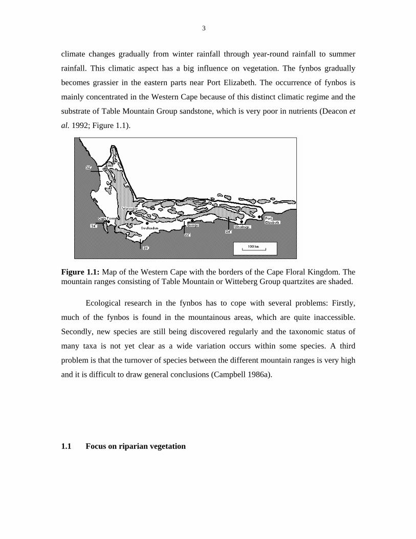
substrate of Table Mountain Group sandstone, which is very poor in nutrients (Deacon et
al. 1992; Figure 1.1).
Figure 1.1: Map of the Western Cape with the borders of the Cape Floral Kingdom. The mountain ranges consisting of Table Mountain or Witteberg Group quartzites are shaded.
Ecological research in the fynbos has to cope with several problems: Firstly,
much of the fynbos is found in the mountainous areas, which are quite inaccessible.
Secondly, new species are still being discovered regularly and the taxonomic status of
many taxa is not yet clear as a wide variation occurs within some species. A third
problem is that the turnover of species between the different mountain ranges is very high
and it is difficult to draw general conclusions (Campbell 1986a).
1.1 Focus on riparian vegetation
4
Within the Fynbos Biome some types of azonal vegetation occur. Azonal vegetation
types are vegetation types that are not dependent on the climatic zone, but are adapted to
specific habitat types that can occur across many different climatic regions and are
vegetated by specialized plant species (Walter 1973). Some examples are saltmarshes,
coastal vegetation, rocky outcrops and aquatic vegetation.
To a lesser extent, riverbanks also belong to this category. Rivers flow through
the vegetation of a biome and contain numerous plant species from it, but they also
generally support their own specific vegetation. Over the whole course of a river the
vegetation around it is influenced by its flood regime. The vegetation associated with a
river in Mountain Fynbos will contain a mixture of typical fynbos elements and non-
fynbos plants adapted to the specific ecological conditions present around a river.
Campbell (1986b) calls this vegetation ‘Closed-scrub fynbos’, but there are few detailed
studies of riverbank vegetation in the Mountain Fynbos to support this structural
definition.
Rivers are currently a big issue in South Africa, which is a fairly arid and
drought-prone country as they form the country’s main source of high quality drinking
water. It is expected that in the near future the water resources in South Africa will
become limited for an increasing population (Boucher & Marais 1993). The Department
of Water Affairs and Forestry endorses a policy that includes sustainable utilization of
water, while the river ecosystem itself is also recognised as a water user (O’Keeffe 1986;
Davies et al. 1993). This principle has subsequently been implemented in the Water Act
of 1995. A well-known success story to increase the supply of water from rivers and
catchments is the Working for Water Project that also provides low-skill jobs for
formerly disadvantaged communities. In this project, alien vegetation is eradicated in
order to increase the runoff in the catchment (Boucher & Marais 1995; Anon. 1999).
The riparian vegetation fulfils an important function in the riverine ecosystem. It
controls the velocity of floodwater and the erosion of the riverbanks, while it also
provides a habitat on its own and adds to the species and habitat diversity of a river
ecosystem (Rogers & Van der Zel 1989).
1.2 Aims of this study

5
A fair number of studies (Boucher 1996; Brown & Day 1995; Brown & Dallas 1998)
have addressed the biological composition and functioning of the foothill and lower river
reaches, due to the direct interference of human infrastructure with the rivers here.
However, very little is known about the upper reaches of the rivers. In order to get a
better picture of the riverine ecosystems of the Western Cape, this study will describe, in
great detail, the flora and vegetation of the Western Cape mountain streams, focusing on
those of the Hottentots Holland Mountains.
This study will benefit the management of the Hottentots Holland Nature Reserve
and other comparable reserves in the southwestern Cape, because the management of
fynbos reserves has for a long time neglected the role of riparian vegetation. This is not
logical when one considers that one of the major functions that the Mountain Reserves
fulfil is to serve as catchments for clean drinking water (Davies et al. 1993). The riparian
vegetation plays a major role in that function. Once more is known about the riparian
vegetation and the ecological processes that shape it, it will be feasible to establish sites
to monitor change due to management practices. When the natural riparian vegetation is
known, it is easy to monitor changes after the natural order has changed due to human
interference and when the ecological processes are known it can be found out what
practices are necessary to restore the natural situation.
This study differs from the broad-scale all-encompassing surveys of mountain
vegetation in that it will concentrate on one habitat complex only. If this approach is
followed through the whole biome, then one can achieve the total categorization of each
habitat type in a specialist way. In this way, it will be much easier to compare vegetation
types across the biome and it will facilitate the classification of the entire biome in the
end. In this way the specific ecological processes that play a role in each habitat complex
can be highlighted.
Chapters 2 and 3 below serve as an introduction to the study area and the methods
used in the study of vegetation. The results of this research project in the Hottentots
Holland Mountains are dealt with in chapters 4 to 8. These chapters are formatted for
publication in scientific journals, so they are slightly different in their layout than the

6
earlier chapters. Chapter 9 contains a synthesis of the results and highlights the most
important conclusions drawn from the study.

7
2. Description of the study area
2.1 Choice of study area
This study aims at investigating the vegetation of some of the Western Cape mountain
streams in detail. The area chosen for this purpose is the Hottentots Holland Mountains in
the southwestern Cape. This area was chosen for the following reasons:
- It is situated in the core area of the Fynbos Biome. The highest species diversity
occurs here and most probably also the highest diversity in vegetation types
(Oliver et al. 1983; Cowling et al. 1992).
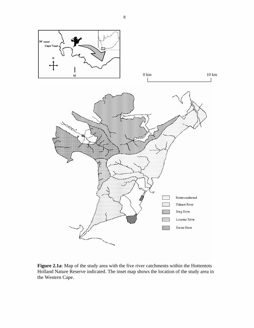
- Five rivers originate in the Hottentots Holland Mountains, two of which have
large catchment areas. The rivers flow in different compass directions: north,
south, east and west (see Figures 2.1 a & b). It is expected that this will result in
strong environmental and climatic gradients.
- Detailed studies have been made on the lower reaches of the rivers that originate
in the Hottentots Holland Mountains, because three of them have been dammed
already and a fourth will be dammed in the near future. The close proximity to the
Cape Metropolitan Area puts a high pressure on the utilization of these rivers to
provide drinking water.
The Hottentots Holland Mountain range is situated southeast of Stellenbosch. Most of the
area currently falls under the jurisdiction of the Western Cape Nature Conservation
Board. The area fulfils different functions. The most important one is the maintenance of
catchments with the best quality drinking water. The Steenbras, Kleinplaas and
Theewaterskloof Dams are all fed by water from the Hottentots Holland Mountains. They
serve as a principle source of water for the Cape Metropolitan Area. For this reason the
vast majority of properties at high altitude are now state owned by and subjected to the
Mountain Catchment legislation (Cape Nature Conservation 1994).
8
Figure 2.1a: Map of the study area with the five river catchments within the Hottentots Holland Nature Reserve indicated. The inset map shows the location of the study area in the Western Cape.
0 km 10 km
9
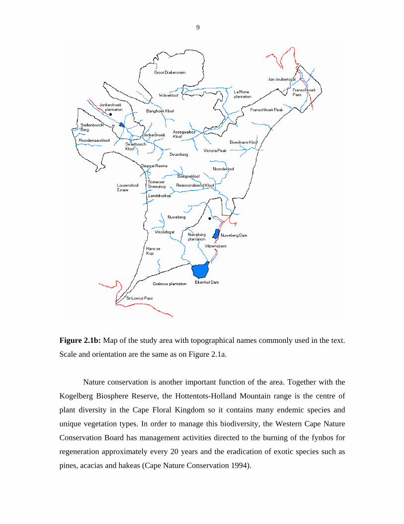
Figure 2.1b: Map of the study area with topographical names commonly used in the text.
Scale and orientation are the same as on Figure 2.1a.
Nature conservation is another important function of the area. Together with the
Kogelberg Biosphere Reserve, the Hottentots-Holland Mountain range is the centre of
plant diversity in the Cape Floral Kingdom so it contains many endemic species and
unique vegetation types. In order to manage this biodiversity, the Western Cape Nature
Conservation Board has management activities directed to the burning of the fynbos for
regeneration approximately every 20 years and the eradication of exotic species such as
pines, acacias and hakeas (Cape Nature Conservation 1994).
10
Another function of the area is recreation. The first section of the Boland Hiking
Trail is situated within the nature reserve. Here visitors can experience the botanical
diversity of the area on several day hikes. There are four mountain huts within the Nature
Reserve where visitors can spend the night: two in Boesmanskloof on the eastern edge of
the park and two on Landdroskop in the central part of the park (Cape Nature
Conservation 1994).
Around the nature reserve there are big areas utilized for wood production. There
are four main Forestry Stations here administered by SAFCOL: Nuweberg in the east,
Grabouw in the south, La Motte near Franschhoek in the northeast, and Jonkershoek near
Stellenbosch in the northwest. Large private plantations are located in the Lourens River
catchment near Somerset West.
There are five major river catchments within the area. Each of these rivers will be
discussed in detail in section 2.7.4.
2.2 Climate
The most significant characteristic that distinguishes the climate of the Fynbos Biome
from that of the rest of the subcontinent is the season in which most precipitation falls.
Within the biome this occurs in winter or year-round, while elsewhere on the
subcontinent it occurs mostly in summer. Detailed accounts about the climate of the
Western Cape and comparisons to that of the rest of the country are given by Schulze &
McGee (1978) and Schulze (1965).
Following the Köppen system (Köppen 1931), the climate in the Westen Cape is
classified as Mediterranean with hot dry summers and mild, wet winters. The code
symbols given to such a climate in Köppen’s (1931) system is Csb, that means a
mesothermal (C) climate with a warm and dry summer with average temperatures above
22° C and relatively wet winters (sb). This is the true Mediterranean Climate and it only
occurs in the western part of the Biome, between Saldanha and the Breede River Mouth
(Boucher & Moll 1981). Other areas in the world, where this kind of climate is found, are
situated around the Mediterranean Basin in Europe and North Africa, in southwestern and
southern Australia, in California, and parts of Chile. In the eastern parts of the Western
11
Cape the climate changes into a steppe climate (Bsk) or a temperate all-year rainfall
climate (Cfb). In the north (the Cedarberg) a Csa climate prevails, which has hotter
summers (Campbell 1983; Schulze & McGee 1978).
Thornthwaite (1948) developed a climatic classification that takes seasonality into
account. He utilizes a climatic water budget and calculates a thermal efficiency index that
relates the temperature to the effective precipitation. Poynton (1971) adapted the
Thornthwaite classification for use in South Africa. He subdivided Thornthwaite’s
mesothermal zones according to the minimum temperature of the coldest month. The
Western Cape falls into Poynton’s warm-temperate and cool-temperate zones, with the
coastal zones being warmer (Schulze & McGee 1978).
Emberger (1955) introduced a pluviometric quotient to classify mediterranean
climates from hyperarid to hyperhumid. He states that winter rainfall and summer aridity
are the two main characteristics of a mediterranean climate. This aridity can be expressed
as a quotient of rainfall and temperature. This pluviometric quotient is expressed as
follows:
22
2000mMRQ
−=
in which R is the year-round rainfall, M the mean maximum temperature for summer and
m the mean minimum temperature for winter. Small values of the pluviometric quotient
represent dry climates while high values represent the wetter climates. The Western Cape
supports climates which are both on the arid extreme of this gradient (in the Knersvlakte
in southern Namaqualand) and on the hyperhumid extreme of the gradient (the Hottentots
Holland Mountains) (Versfeld et al. 1992). Emberger (1955) considered the climate to be
mediterranean when the ratio of summer rainfall to average mean maximum temperatures
for the summer months is less than 7. Lower values signify more pronounced summer
droughts. The Swartboschkloof weather station has a ratio of 6.5 which places this area in
the mesic extreme of a mediterranean climate. Other parts of the world, that have a
similarly high rainfall, have a quite different vegetation cover (Versfeld et al. 1992).
Another feature in which the Western Cape’s climate differs from that of the rest
of the subcontinent is the unpredictability of weather conditions. The high variation and
12
unpredictability of the weather in the area is caused by a combination of coastal
mountains which cause windward-leeward patterns and the warm Agulhas current in the
south in contrast with the cold Benguela current in the west, which make temperatures
highly dependent on wind direction (Deacon et al. 1992).
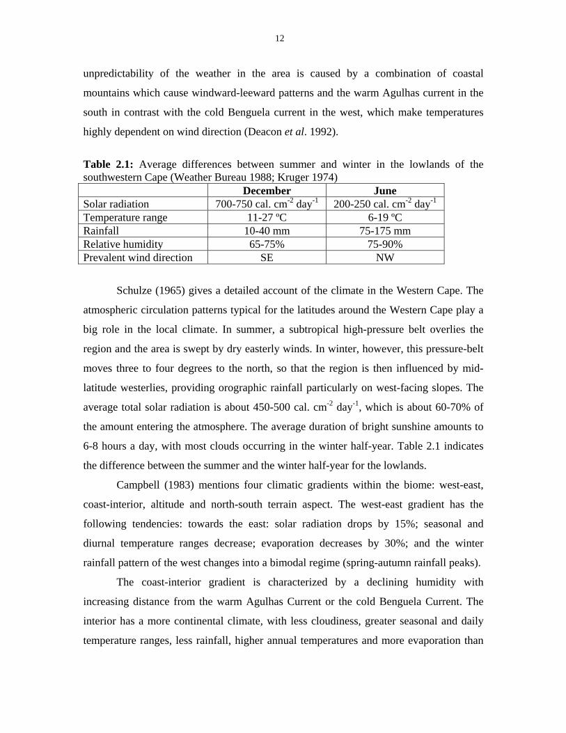
Table 2.1: Average differences between summer and winter in the lowlands of the southwestern Cape (Weather Bureau 1988; Kruger 1974) December June Solar radiation 700-750 cal. cm-2 day-1 200-250 cal. cm-2 day-1 Temperature range 11-27 ºC 6-19 ºC Rainfall 10-40 mm 75-175 mm Relative humidity 65-75% 75-90% Prevalent wind direction SE NW
Schulze (1965) gives a detailed account of the climate in the Western Cape. The
atmospheric circulation patterns typical for the latitudes around the Western Cape play a
big role in the local climate. In summer, a subtropical high-pressure belt overlies the
region and the area is swept by dry easterly winds. In winter, however, this pressure-belt
moves three to four degrees to the north, so that the region is then influenced by mid-
latitude westerlies, providing orographic rainfall particularly on west-facing slopes. The
average total solar radiation is about 450-500 cal. cm-2 day-1, which is about 60-70% of
the amount entering the atmosphere. The average duration of bright sunshine amounts to
6-8 hours a day, with most clouds occurring in the winter half-year. Table 2.1 indicates
the difference between the summer and the winter half-year for the lowlands.
Campbell (1983) mentions four climatic gradients within the biome: west-east,
coast-interior, altitude and north-south terrain aspect. The west-east gradient has the
following tendencies: towards the east: solar radiation drops by 15%; seasonal and
diurnal temperature ranges decrease; evaporation decreases by 30%; and the winter
rainfall pattern of the west changes into a bimodal regime (spring-autumn rainfall peaks).
The coast-interior gradient is characterized by a declining humidity with
increasing distance from the warm Agulhas Current or the cold Benguela Current. The
interior has a more continental climate, with less cloudiness, greater seasonal and daily
temperature ranges, less rainfall, higher annual temperatures and more evaporation than
13
the coastal areas. The mountains near the coast have considerable precipitation from
mists even in the dry season (Campbell 1983).
In mountainous areas like the Western Cape climatic conditions differ
considerably locally and mesoclimate plays a major role in determining the vegetation.
Different slopes receive different amounts of sunlight, with northern slopes heating up
more than the southern slopes, depending on their steepness and on the season. This
results in air currents moving up-slope by day. At night, cold air from near the ground
flows down the slopes. This causes a downward movement during the night and an
upward movement during the day. With increasing altitude, mean annual temperatures
decrease, pan evaporation decreases, rainfall increases and the likelihood for mists and
snow increase (Campbell 1983). 2.2.1 Temperature
Fuggle & Ashton (1979) located 120 weather stations in the biome where temperature is
recorded, but very few of these are situated in the mountains. Mean annual temperatures
throughout the region are close to 17°C. Temperature ranges are bigger inland than near
the coast. The highest summer temperatures recorded (higher than 30°C) are from the
Great Karoo as well as from the major river basins. These places also experience the
coldest winter temperatures. Occasionally high temperatures occur next to the coast
associated with certain off-shore winds. Frost is a rare phenomenon near the coast but is
common in July and August in the interior (Fuggle & Ashton 1979).
A temperature gradient with altitude for the southwestern Cape was calculated by
the South African Weather Bureau. It became apparent that temperatures decrease by
0.5°C per 100 m increase in altitude throughout the year. Temperature lapse rates are
more consistent than those for rainfall (A. Chapman, CSIR Stellenbosch, pers. comm.).
High temperatures and arid conditions combined with strong winds are an
important cause of extensive veldfires that occur throughout the biome, particularly in
late summer and autumn. These play an important role in the life cycle of fynbos plants
(Fuggle & Ashton 1979).
14
There is not much specific temperature data available from the Hottentots Holland
Mountains. Versfeld et al. (1992) provide some data for Swartboskloof. Temperatures
have an average of 16.2°C (range: 0.2°C ∠ 39°C) at the Jonkershoek Weather Station
(305 m alt.). Above 600 metres occasional snowfalls occur in winter (Versfeld et al.
1992).
2.2.2 Solar radiation
Solar radiation is a fundamental climatic parameter because of its influence on near
surface air temperatures, soil temperatures, evaporation and water vapour deficit. It is
highly variable in mountainous regions. The intensity is influenced, inter alia, by aspect
and slope, but also by surrounding geomorphology. Thus narrow valleys are exposed to
less direct sun rays than mountain peaks and can lose several hours of sunshine in a day
(Kruger 1974). North- and south-facing slopes of less than 30 degrees do not differ that
much in their daily receipt of sunshine during summer, but in winter north-facing slopes
receive three to five times as much solar radiation as equivalent slopes facing south.
2.2.3 Precipitation and evaporation
Precipitation is mostly in the form of rain with more than 60% falling between April and
September. Snow and hail are quite rare and occur mostly at high altitudes. Most
mountains in the Western Cape have a rainfall between 1000 and 2000 mm per year, but
in the wettest areas (like the Hottentots Holland Mountains) it might exceed 3000 mm
(Schulze 1965). Most lowland locations receive much less, up to 750 mm near the coast,
and mostly less than 400 mm in the intermontane valleys (Fuggle & Ashton 1979).
15
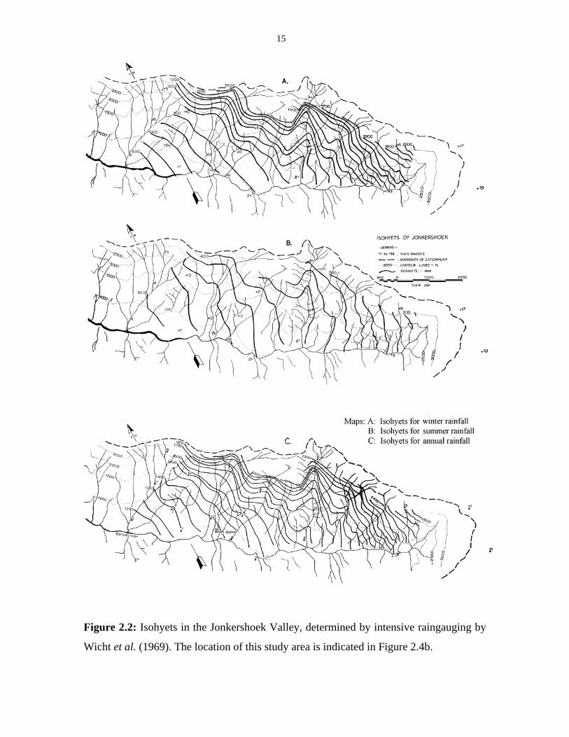
Figure 2.2: Isohyets in the Jonkershoek Valley, determined by intensive raingauging by
Wicht et al. (1969). The location of this study area is indicated in Figure 2.4b.
16
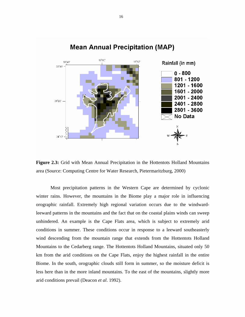
Figure 2.3: Grid with Mean Annual Precipitation in the Hottentots Holland Mountains
area (Source: Computing Centre for Water Research, Pietermaritzburg, 2000)
Most precipitation patterns in the Western Cape are determined by cyclonic
winter rains. However, the mountains in the Biome play a major role in influencing
orographic rainfall. Extremely high regional variation occurs due to the windward-
leeward patterns in the mountains and the fact that on the coastal plains winds can sweep
unhindered. An example is the Cape Flats area, which is subject to extremely arid
conditions in summer. These conditions occur in response to a leeward southeasterly
wind descending from the mountain range that extends from the Hottentots Holland
Mountains to the Cedarberg range. The Hottentots Holland Mountains, situated only 50
km from the arid conditions on the Cape Flats, enjoy the highest rainfall in the entire
Biome. In the south, orographic clouds still form in summer, so the moisture deficit is
less here than in the more inland mountains. To the east of the mountains, slightly more
arid conditions prevail (Deacon et al. 1992).
17
Schulze (1965) indicates a strong gradient in rainfall with increasing altitude. On
an average annual basis he calculates a gradient of 50 mm increase per 300 m increase in
altitude. The overall rainfall pattern in the mountains, however, is difficult to predict and
very irregular. It is mainly dependent on the exposure of slopes to northwesterly and
southwesterly winds. Mountains can also receive a lot of precipitation from mist that is
not registered in the rain gauges (Kerfoot 1968; Fuggle & Ashton 1979).
Wicht et al. (1969) have done an extensive study of rainfall patterns in the
mountains surrounding the Jonkershoek Valley. The maps with isohyets that they
produced for the valley are presented in Figure 2.2. From these maps it can be seen that
rainfall patterns do not have a very reliable relationship with altitude in the way Schulze
(1965) proposed. The data from the many weather stations used in this study and an
additional weather station that operated on top of Victoria Peak in the eighties (G.G.
Forsyth, CSIR Stellenbosch, pers. comm.) formed the basis for the rainfall grid that was
produced by the Computing Centre for Water Research (CCWR) and that is illustrated in
Figure 2.3. The methodology to extrapolate rainfall point data to a grid is provided by
Dent et al. (1987).
In July, orographic rains occur over the west-facing slopes of the Hottentots
Holland Mountains. A moisture surplus remains in winter only in the area south of 33°S
and west of 20°E (Deacon et al. 1992). Southeasterly winds rarely bring rain to the flats,
and they generally create arid conditions and föhn-like ‘bergwinds’, after which
temperatures increase in Jonkershoek (Wicht et al. 1969).
The Jonkershoek Valley shows a very strong orographic gradient. Rainfall
increases from 786 mm in Stellenbosch (100 m alt.) to 3625 mm on the Dwarsberg
Plateau (1220 m alt.). This is the highest recorded rainfall in the whole of South Africa.
The increase in rainfall with altitude is also evident in the Swartboskloof subcatchment in
Jonkershoek where it increases from 1523 mm at 305 m altitude to 2815 mm at 910 m
altitude. About 75% of this rain falls in the period April-September. The typical pattern
of rainfall is one of light to steady rain when frontal air masses arrive from the northwest
followed by sharp intermittent showers as the wind swings to the southwest and
southeast. Annual evaporation generally exceeds rainfall by 25% (Versfeld et al. 1992).
18
1. 2.
3. 4.
5. 6.
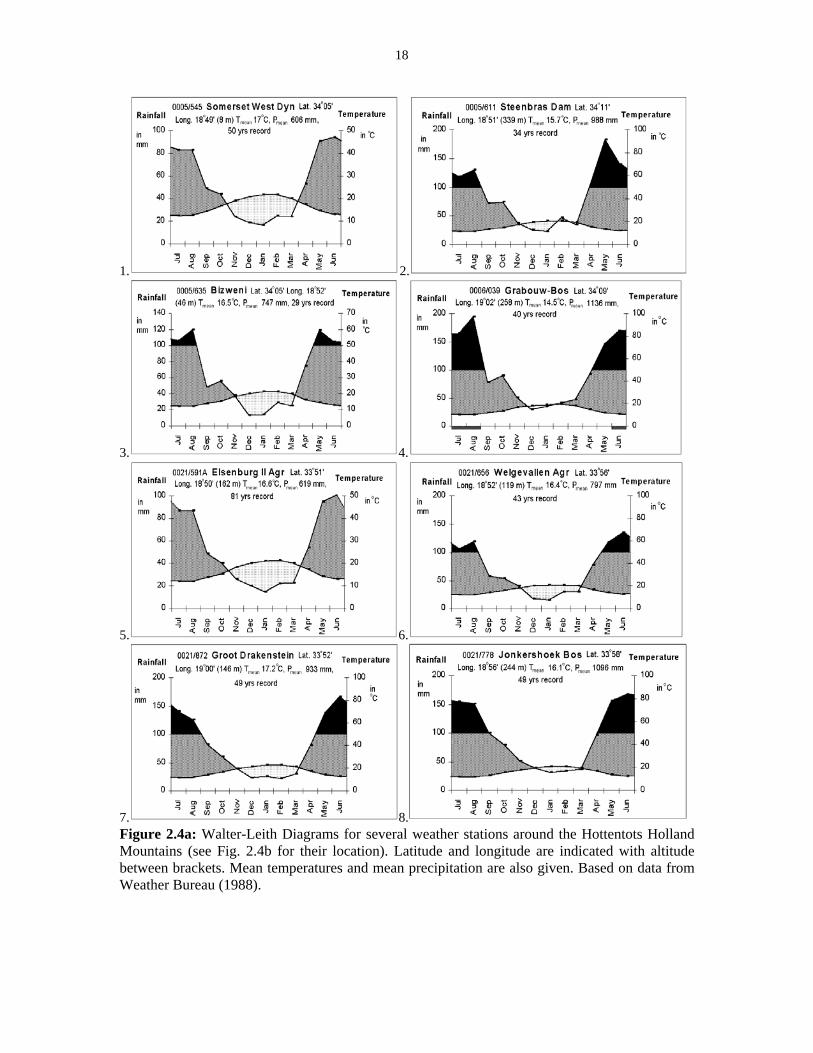
7. 8. Figure 2.4a: Walter-Leith Diagrams for several weather stations around the Hottentots Holland Mountains (see Fig. 2.4b for their location). Latitude and longitude are indicated with altitude between brackets. Mean temperatures and mean precipitation are also given. Based on data from Weather Bureau (1988).
19
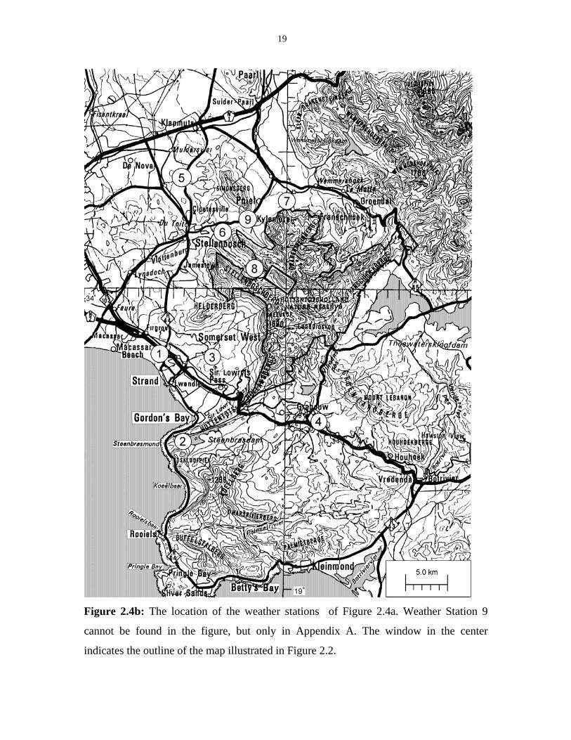
Figure 2.4b: The location of the weather stations of Figure 2.4a. Weather Station 9
cannot be found in the figure, but only in Appendix A. The window in the center
indicates the outline of the map illustrated in Figure 2.2.
20
Evaporation is dependent on many factors. The saturation deficit, which is based
on temperature and relative humidity, represents the amount by which atmospheric water-
vapour-pressure falls short of saturation and shows the evaporative potential of the
atmosphere. Actual evaporation is also dependent on solar energy and on the wind.
Values of 2000 mm per year are recorded from the interior valleys and in the
southwestern Cape, with about 40% occurring in summer. Towards the east, this value
decreases. There is no data available for mountain locations, and it is likely that big
differences exist between slopes of different aspect and with different moisture regimes
(Fuggle & Ashton 1979). Figure 2.4 illustrates the Walter-Leith diagrams of the weather
stations surrounding the Hottentots Holland Mountains. More detailed information about
these weather stations can be found in Appendix A.
Tyson (1978) investigated the changes in rainfall patterns in South Africa. He
concluded that there are oscillations in rainfall within a 20-year period. There is no
progressive trend towards aridification in the Western Cape and historical data on climate
can still be useful. Today, however, there might be an effect of global warming on the
climate in the Cape, but this still has to be proven (Rutherford et al. 1999).
2.2.4 Wind
As shown above, wind plays a major role in determining the weather in the Western
Cape. The distribution of precipitation on a mountain depends mainly on the wind. Rain
and snow will mainly fall in the wind shadows. Westerly winds blow cold air from the
Atlantic Ocean inland, while easterly winds bring warm air overland from the Indian
Ocean (Deacon et al. 1992).
A ridge of high pressure extends from the South Atlantic anticyclone to the Cape
coast. In summer, this ridge lies further to the south, at 37°S, which promotes the dry
easterly winds, while in winter the ridge is situated at 32°S and westerly winds dominate.
In the latitudes in between an unstable westerly wind gives rise to frontal depressions,
ridging anticyclones, coastal lows and cut-off lows which cause highly variable day-to-
day conditions of wind, moisture and temperature (Deacon et al. 1992).
21
Extreme wind conditions appear all along the coastal plains, mostly with wind
speeds above 30 km/hour. The highest wind velocities occur near Bredasdorp. These high
velocities occur here mostly in summer, whereas the mountain tops have a maximum for
wind speed in winter (Deacon et al. 1992).
Winds mainly blow in directions parallel to the coast, so on the south coast there
is polarization along an E-W axis, and on the west coast along a NW-SE axis. Further
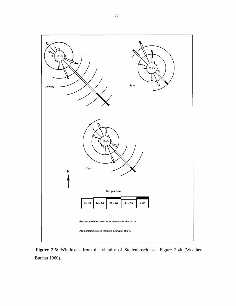
inland, there are more variations in wind direction (Deacon et al. 1992). Figure 2.5
illustrates annual and seasonal windroses for the surroundings of Stellenbosch based on
data from the Weather Bureau (1960).
Dominant winds in summer are from the southeast, while in winter they blow
from the northwest and carry rain. Warm northeasterly winds (‘bergwinds’) occur
especially in late summer. They are characterized by sudden increases in temperature and
decreases in humidity. This increases the likelihood of wildfires (Versfeld et al. 1992;
Kruger 1978b).
2.3 Geology and geomorphology
The distinct climate in the Western Cape is not sufficient to explain the occurrence of
unique vegetation types here. The existence of a winter rainfall climate is geologically
relatively young, while many taxa that occur in the Fynbos Biome are much older. The
mountains and geological formations will also play an important role in explaining why
the fynbos only exists in its present refuge (Deacon et al. 1992).
22
Figure 2.5: Windroses from the vicinity of Stellenbosch, see Figure 2.4b (Weather
Bureau 1960).
23
2.3.1 Geology
The rock formations in the Fynbos Biome have different origins. The oldest ones
belong to the Malmesbury, Kango, Kaaimans and Gamtoos Groups. The sediments in
these groups were folded during the Late Precambrium, in a period of mountain building
that is known as the Saldanian orogeny. Their lithology ranges from clays to
conglomerates and they were intruded by granites of the Cape Granite Suite. Erosion
reduced these Cape Mountains to a level plain and then they were covered again by
sediments of subsequent groups. Of these old sediments, only the Malmesbury Group and
the Cape Granites are still found on the surface over large areas. These Precambrian
rocks, together with the granites, are different from the later sediments in that they are
base rich. On weathering, the predominantly clayey substrates release exchangeable
cations, such as calcium, potassium, magnesium and sodium. These are important
nutrients for the plants and they play a major role in the formation of soils (Deacon et al.
1992).
The newer mountain ranges that were planed over the Precambrian rocks
consisted mainly of hard quartzitic rocks belonging to the Cape Supergroup. From old to
new these are: the Table Mountain Group, the Bokkeveld Group and the Witteberg
Group. The Table Mountain Goup and Witteberg Group are of an arenaceaous
(sandstone) origin and are acidic and poor in nutrients. The Bokkeveld Group has an
argillaceous (mudstone) facies. Each group can be divided into strata with distinctive
lithologies, which are defined as formations. The formations in the Cape Supergroup
were formed in the period from the Late Ordovicium until Carboniferous, between 450
and 300 million years ago (Deacon et al. 1992).
The Cape Fold Mountains consist of hard quartzitic rocks belonging either to the
Table Mountain Group or the Witteberg Group. The synclinal and fault valleys often
have other geological units in the substrate such as the highly weatherable slates and
phyllites of the Bokkeveld Group, or, as in the case of Jonkershoek, granites of the Cape
Granite Suite (Lambrechts 1979).
24
The Table Mountain Group contains five different formations, some consisting of
shale or tillite, others consisting of sandstone. They are listed here from the oldest to the
youngest substratum. The Graafwater Formation forms the lower altitude shale-bands.
The Peninsula Formation consists of sandstones and is locally more than 1700 metres
thick. The Pakhuis Formation consists of tillite of glacial origin. The Cedarberg
Formation always accompanies the Pakhuis Formation and consists of a shale-band at
high altitude, about 50 metres thick. The Nardouw Formation is formed by the sandstones
that occur above these shale-bands and can be 1000 metres thick (De Villiers et al. 1964).
The Karoo Formations have a much younger origin. They are presently found
only in the more inland areas of South Africa and are not present in the study area.
During the deposition of the Dwyka Formation, the oldest of the Karoo Formations, the
Karoo and the Cape were folded in an episode of mountain building known as the Cape
orogeny. This happened in the Permian and Triassic, between 278 and 215 million years
ago. The Cape Fold Mountains rose and formed a source of sediments that were
deposited in the Karoo basin. The Dwyka Formation was followed by, respectively, the
Ecca, Beaufort and Stormberg Formations and the Karoo sequence was concluded in the
Jurassic (about 150 million years ago). After this, Gondwanaland, the big continent of the
Southern Hemisphere, started to break up.
Formations from the Cretaceous Period in South Africa are known from near the
shore and can be regarded as relicts of the continental breakup. There are alluvial gravels,
colluvial screes and coastal deposits that originate from the Cainozoic. These deposits are
not particularly thick but they are important ecologically as they form the limestones near
Bredasdorp and the coastal sands on the West Coast, both of which have unique
vegetation types growing on them (Deacon et al. 1992).
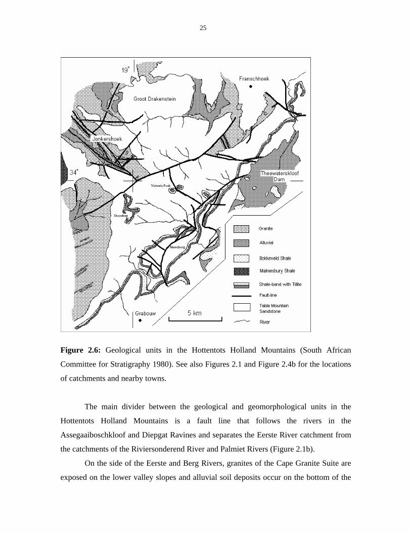
In the Hottentots Holland Mountains different geological units are exposed on the
eastern versus the western slopes. The distribution of the different strata are illustrated in
Figure 2.6. The mountains are mainly formed by sandstones of the Table Mountain
Group, which are extremely poor in nutrients.
25
Figure 2.6: Geological units in the Hottentots Holland Mountains (South African
Committee for Stratigraphy 1980). See also Figures 2.1 and Figure 2.4b for the locations
of catchments and nearby towns.
The main divider between the geological and geomorphological units in the
Hottentots Holland Mountains is a fault line that follows the rivers in the
Assegaaiboschkloof and Diepgat Ravines and separates the Eerste River catchment from
the catchments of the Riviersonderend River and Palmiet Rivers (Figure 2.1b).
On the side of the Eerste and Berg Rivers, granites of the Cape Granite Suite are
exposed on the lower valley slopes and alluvial soil deposits occur on the bottom of the
26
valley. In Jonkershoek, many faultlines occur and are accompanied by cataclasite. Small
bands of dolerite are also found in the granite. The granite at the head of the valley,
towards the Dwarsberg, is of a different structure to the granite found elsewhere. It is an
equigranular granite or aplogranite in contrast to the porphyritic granite found towards
Stellenbosch. In the Berg River catchment near Franschhoek, other porphyritic granites
are found in the area that is covered by the La Motte plantation (South African
Committee for Stratigraphy 1980). Rubble from the surrounding sandstone slopes cover
part of the valleys, where they overly the granite, which results in a mixed substrate.
The mountains on the side of the Palmiet and Riviersonderend Rivers, on the
other side of the dividing faultline, only consist of materials of the Table Mountain
Group. These are mainly sandstones; however, thin bands of tillite and shale are exposed
over the whole range from Sir Lowry’s Pass to Franschhoek Pass and near the mountain
tops of Somerset Sneeukop, Victoria Peak and Emerald Dome. These bands always occur
together but their continuity is broken up by several fault lines that cross the area (South
African Committee for Stratigraphy 1980). They are also often overlain by sandstone
rubble.
2.3.2 Geomorphology
The shape of the earth’s crust is influenced by a series of factors, of which the most
important are the geological substrate, the elevation and the climate. Different layers are
subject to different rates of chemical and mechanical weathering. The elevation is
important because it determines the hydrology of the area compared to the surrounding
areas. The climate is all-important because it determines the rate of weathering and the
growth of vegetation, which in itself also has an influence on erosion.
The rivers, which form the central part of this study, are also one of the major
agents in shaping the landscape. The geological substrate is important as it defines how
the river network will develop. On homogeneous substrates this network will develop in
a dendritic pattern, in such a strict way that one can simulate its course by computer.
However, homogeneous substrates rarely stretch over great distances, so the kind of
branching system that develops is dependent on the geology of the area. Harder and
27
softer layers, intrusions and other geological structures all have their influence on the
river network.
In the upper reaches of the river erosive forces dominate and here the river cuts
deeply into the substrate. The erosive force of water mainly comes from the sediment
load. The erosion directly inflicted by the river is called vertical erosion. The slopes of
the gorges that come into existence after vertical erosion are subject to colluvial
weathering with lateral subsidence into the river. On very hard sandstone rocks, for
instance, there is hardly any lateral subsidence into the river, which is why very steep
gorges occur in these situations in the Hottentots Holland Mountains.
Eventually, though, in every river, vertical erosion slows down and lateral
subsidence becomes the most dominant erosive force. In a mature landscape weathered
material from the hillslopes settles down at the foothills to form a pediment. Valleys
become broader and flatter and planation takes place until a new geological upliftment
takes place. This is called the peniplanation cycle (King 1967).
The African continent in general is characterised by an extreme form of planation
that took place after the break-up of Gondwanaland and the deposition of the Karoo
sediments. This planation results in the flat landscapes that occur all over the continent.
In areas that have a lower elevation this flatness is most obvious, as in the Kalahari
Desert. In the Pliocene, however, the interior plateau of the continent was elevated for
more than thousand metres while the coastal areas kept their low elevation. This process
of cymatogeny resulted in the phenomenon that is now called the Great Escarpment
(King 1967, 1978; Partridge 1997). The Great Escarpment is found much further inland
than the Cape Mountains which support the fynbos vegetation.
The Western Cape is characterized by the Cape Folded Belt, where a number of
mountain ranges occur parallel to the coast. There are two main zones of folding: in the
western part there are mountain ranges running north-south concave to the west and in
the eastern part there are mountain ranges running east-west, slightly concave to the
south. South from Tulbagh the folding takes many directions. This is probably because of
the two zones meeting each other here. The present landscape has probably existed since
the mid-Cretaceous, after the Cape Orogeny had taken place in Permian and Triassic
28
times and the Cape rivers had excavated the mountain ranges and deposited their
sediments in the Karoo (Wellington 1955; King 1962; Lambrechts 1979).
The Table Mountain Group sandstone is a good water-carrier that allows water to
penetrate to considerable depths. In several places in the Western Cape, at the junction of
the Table Mountain Group sandstone and the Bokkeveld Group shales, warm-water
springs can be found, for example at Caledon, Montagu and Citrusdal (Wellington 1955).
Few detailed geomorphological studies have been done to outline the influences
of the Western Cape rivers on their landscape. A few studies have been done on the
Eerste River in the surroundings of Stellenbosch. Beekhuis et al. (1944) give a detailed
account of the whole course of this river. They describe some of the alluvial fan-cores
that some tributaries in the Jonkershoek Valley have created at the point where they enter
the main stream. The fans that have been created at the base of the Swartboskloof and
Disa Kloof streams are so thick that they have partially dammed the river, creating a
marsh where the current slows down. Above this marsh the river is slow flowing while
below it the river flows rapidly and has cut a deep channel.
The alluvial soils around Stellenbosch are the subject of Söhnge’s (1981) study.
The town of Stellenbosch is built on an alluvial fan with its apex towards the Jonkershoek
Valley. Three different periods of deposition have resulted in the formation of three
terraces. The oldest deposits are from Mid-Pliocene and probably relate to older tributary
courses. During the formation of the two other deposits the Eerste River changed its
course.
2.4 Soils and pedogenesis
There is no unified international terminology for soil description. Most versions are
variants of the approach presented in United States Department of Agriculture (1951).
The classification of the different soil profiles does not have an international standard
either, however the United States Department of Agriculture (1975) system is widely
applicable. Many regions and nations have their own classification systems (Ball 1986).
The South African classification of soil types is outlined by the Soil Classification
Working Group (1991). This is the classification followed in this study.
29
Many of the soils found in the mountains are shallow, weakly developed soils
which are termed lithosols. Podzolization is the most important soil-forming process
here, although Campbell (1983) argues that its impact is usually overestimated. In the
podzolization process substances such as iron, aluminium and organic matter are leached
from the A-horizon and accumulate in the podzolic B-horizon which, as a result, becomes
darker in colour. The soils are very poor in plant nutrients, particularly in phosphates.
Highly variable and localized conditions of soil depth, soil moisture and aspect result in
many different microhabitats. In contrast with the soils of the coastal plains, which are
base rich, the montane soils favour many specialist species (Deacon et al. 1992).
Campbell (1983) found three dominating soil types throughout the mountainous
regions of the Cape. These are the Mispah, Glenrosa and Cartref Forms. They are all
litholic and represent the shallower soils (less than 0.40 m deep). The soil type is largely
determined by the geology (see also Ball 1986). The Cartref type usually occurs at the
higher altitudes on the coastal mountains. The Glenrosa and Mispah soils occur in the
better drained slopes or at lower altitudes with north aspects. They also dominate the
mountain ranges of the interior on the Witteberg Group quartzites. Of these three most
common soil types, it is only the Glenrosa Form that also occurs to a reasonable extent on
non-quartzite substrates, particularly on shales. The soils on the southerly aspects, the
gentler slopes and the lower altitudes throughout the Cape generally have better
developed profiles. Here the Clovelly, Hutton and Oakleaf Forms can be found
(Campbell 1983).
The main factor that determines the soil type in the mountains is the rainfall.
Where rainfall is abundant, soils are leached and poor in iron oxides. Where rainfall is
low, the soils are leached to a lesser extent and are rich in iron oxides. The common soil
types on mountain slopes in the south of the region, where rainfall is abundant, are the
very shallow sandy soils of the Mispah, Houwhoek and Cartref Forms. These soils often
contain varying amounts of stone that are coarser than 10 mm in diameter. In the drier
areas to the north of the Hottentots Holland Mountains, yellow to yellowish red soils of
the Clovelly and Hutton Forms are found. They can also be found at high altitudes with
much rainfall, but only locally in iron-rich strata on higher slopes (Lambrechts 1979).
30
Campbell (1983) discusses the correlation between climate, weathering and
pedogenesis within the Fynbos Biome. Because of lower plant cover and higher
evaporation on northern slopes one can expect lower rates of chemical weathering, a
higher degree of sheet erosion and minimal soil development here (Bond 1981). In the
north-western parts of the Biome, plant cover is low and rock and debris accumulations,
talus and soil creeps are widespread (Campbell 1983). In the south the debris mantle
appears to be stable and is well vegetated.
Kruger (1974) suggests that fertility in quartzites is mainly determined by plant
remains in the soil. Campbell (1983) argues that fertility is largely dependent on texture.
Many non-quartzite soils have a finer texture and also a higher fertility (Cowling 1984).
Kruger (1974) found the Hutton and Clovelly Forms to be associated with shale-
bands. He also found the Dundee Form on young stratified alluvium in drainage
channels. Fry (1987) gives a description of different catenas (soil gradients) that occur in
Swartboskloof in the Hottentots Holland Mountains. These soil gradients can be
extrapolated to the entire mountain range, because both dominant geological substrates
(granite and sandstone) are found in Swartboskloof. Soils on granites and shales have a
better developed structure and contain more organic carbon in humid places than the soils
derived from sandstone. On sandstone, the soil catena from downslope to upslope
situations is generally Constantia, Clovelly, Hutton, Glenrosa and Mispah. In lowlands or
depressions the catena is formed by a succession of Fernwood (dry phase), Cartref,
Houwhoek and Lamotte Forms in places where podzolisation dominates and by
Fernwood (wet phase), Avalon, Longlands and Westleigh Forms where hydromorphic
processes dominate.
On granite slopes, the catena follows the gradient of Clovelly, Hutton, Glenrosa
and Mispah Forms. In specific situations other soil types can occur, such as Swartland
and Sterkspruit Form soils occurring in the concave lower slope positions with Estcourt
and Kroonstad Forms on the well-drained slopes immediately above. In humid
environments the catena tends to be towards the Magwa, Nomanci, Glenrosa and Mispah
Forms. In many lower-lying areas a mixture of granite and sandstone parent material
occurs as rubble from the erosion of upper slopes.
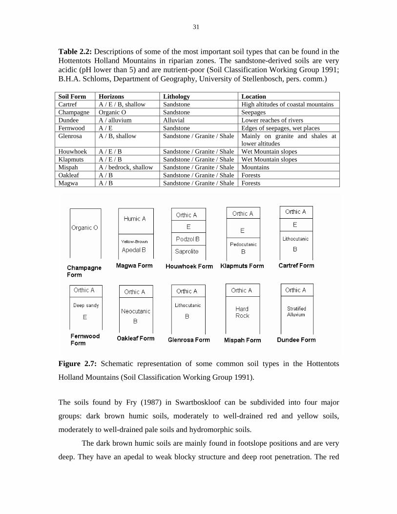
31
Table 2.2: Descriptions of some of the most important soil types that can be found in the Hottentots Holland Mountains in riparian zones. The sandstone-derived soils are very acidic (pH lower than 5) and are nutrient-poor (Soil Classification Working Group 1991; B.H.A. Schloms, Department of Geography, University of Stellenbosch, pers. comm.) Soil Form Horizons Lithology Location Cartref A / E / B, shallow Sandstone High altitudes of coastal mountains Champagne Organic O Sandstone Seepages Dundee A / alluvium Alluvial Lower reaches of rivers Fernwood A / E Sandstone Edges of seepages, wet places Glenrosa A / B, shallow Sandstone / Granite / Shale Mainly on granite and shales at
lower altitudes Houwhoek A / E / B Sandstone / Granite / Shale Wet Mountain slopes Klapmuts A / E / B Sandstone / Granite / Shale Wet Mountain slopes Mispah A / bedrock, shallow Sandstone / Granite / Shale Mountains Oakleaf A / B Sandstone / Granite / Shale Forests Magwa A / B Sandstone / Granite / Shale Forests
Figure 2.7: Schematic representation of some common soil types in the Hottentots
Holland Mountains (Soil Classification Working Group 1991).
The soils found by Fry (1987) in Swartboskloof can be subdivided into four major
groups: dark brown humic soils, moderately to well-drained red and yellow soils,
moderately to well-drained pale soils and hydromorphic soils.
The dark brown humic soils are mainly found in footslope positions and are very
deep. They have an apedal to weak blocky structure and deep root penetration. The red
32
and yellow soils are very diverse. They are derived from quartzites or from a mixture of
granite and quartzite. The Glenrosa Form occurs on footslopes and is very shallow. The
most important soil form in the group with pale soils is the Fernwood Form of which two
phases are recognized: the grey and pale Fernwood Forms. They are both found on
footslopes. The hydromorphic soils contain mottling in the B-horizon. The A-horizon is
dark brown. Descriptions of some of the different soil types that can be found in the
Hottentots Holland Mountains are presented in Table 2.2 and in Figure 2.7.
2.5 Archaeological to recent history
Africa is the continent in which the human species has evolved. The oldest traces of
human settlement in the Western Cape are in the form of artefacts, because skulls and
bones tend to disintegrate under the acidic conditions which are predominantly found
through the biome. There have been few fossil findings, mainly in deeper soil layers that
contain calcareous material. There are discontinuities between these and later findings
which indicate that the climate has probably not always been favourable for human
settlement (Deacon 1992).
2.5.1 The San and Khoikhoi
In the Late Stone Age the people living in the Western Cape were hunter-gatherers and
many of the artefacts found from them suggest that their life-style was in many ways
similar to that of many San people in modern-day Botswana. The many fossils that have
been found from the early Holocene (10 000 years ago) suggest that they lived in
territorially organized groups. They probably used fire-stick farming to encourage natural
fields of geophytes, and they killed the small antelope in the surrounds of these patches.
The population grew steadily until two thousand years ago when a new way of life was
established in the Fynbos Biome, namely herding. The first practice of domestication of
sheep and cattle originated in the Middle East, from where it quickly spread into North
Africa, but took nearly 6000 years for these practices to spread over the entire continent,
including the Western Cape. Herding was associated here with the people who spoke
33
Khoikhoi. In some areas with suitable conditions stock farming was established. When
external trade became important, large herds were recorded like one of 20 000 cattle that
was driven to Table Bay in 1652. The hunter-gatherer life-style was regularly in conflict
with the herding life-style, but in general the two peoples of San and Khoikhoi cultures
managed to live together and this is how the first Europeans found the Cape in the 16th
century (Deacon 1992).
2.5.2 Early settlers
The first Europeans to arrive at the Cape were Portuguese explorers. Later on, Europeans
of different nationalities used the Cape as a stop-over on route to Eastern Asia, and they
traded with the Khoikhoi for their supplies. It was the Dutch who took the decision to
start a supply station at the Cape in order to control this kind of trade in the face of
English and French competition. The Khoikhoi were not united in their resistance to the
occupation of their traditional lands and their society was rapidly disrupted. Although
Khoikhoi resistance was heavily suppressed by Europeans, the settlers took over several
elements of the Khoikhoi culture like nomadism and veld management practices and this
facilitated expansion of the colony (Deacon 1992).
The mountains of Hottentots Holland formed the border between the Cape Colony
and the vast inland part of South Africa. That is why they were named ‘the mountains of
Africa’. In 1663 the land surveyor Hendrik Lacus was the first of the colonists to cross
this mountain range and to see the other side of the mountains. He made use of a little
track in a gorge near the place where Sir Lowry’s Pass is today. The European colonists
called this track the Elandspad. It took many years before others followed. On the lower
slopes of the Hottentots Holland Mountains some important outposts of the Cape Colony
were established (Heap 1993). In the meanwhile the Khoikhoi crossed the mountains
quite often to look for new pastures for their cattle. When the colonists started to trade
with the Khoikhoi they started to make use of the Elandspad more often and a tollhouse
was established at the beginning of the kloof. Nowadays the traces of the many oxwagons
that passed here are still visible and it is a declared National Monument (Cape Nature
Conservation 1994).
34
A second pass over the Hottentots Holland Mountains in the Western Cape was
built in 1819. A Franschhoek farmer had built a path through the mountains from
Franschhoek to the Viliersdorp side. This path, however, was very dangerous and soon a
new track was built by the Cape administration. In 1825 the Franschhoek Pass was
opened and this is now recognized as South Africa’s oldest mountain pass (Cape Nature
Conservation 1994).
2.5.3 Land use
Nowadays the Hottentots Holland Nature Reserve is used mainly as a catchment area for
clean potable water, but also as a nature reserve and a recreational area. The surrounding
areas are used mainly for agriculture. In the west there are mainly winelands and in the
southeastern parts there are orchards with apple trees. Directly on the border of the
reserve there are large pine plantations for wood production. This makes the mountain
vegetation quite susceptible to alien invaders. A map illustrating basic land use patterns is
presented in Figure 2.8.
2.6 Botanical background
In his survey of the general veld types and their potential for agriculture Acocks (1953,
1975) divided the vegetation of the Fynbos Biome into three groups, two of which were
dominant in the mountains: Macchia and False Macchia. He changed the word Macchia
into Fynbos in a later publication (Acocks 1988). He recognised, however, that this
division was quite coarse and preliminary. Azonal vegetation types like riparian
vegetation were not described. After the publication of research resulting from the
Fynbos Biome Project, the knowledge of the biogeography and ecology of fynbos was
deepened.
2.6.1 Origins of the Cape Flora
35
Different origins for the flora of the Cape are indicated by track analysis. In track
analysis, the extra-regional distributions of taxa are examined to determine which areas
share a floristic component with the area in question. In this way it can be seen which
other floras were previously in contact with the Cape Flora. This can be matched to the
knowledge from palaeoclimates and palaeogeography (Stott 1981).
A track is defined by the distribution of a taxon. In European literature, it is also
known as a ‘geo-element’ (Walter 1973). If several tracks coincide they form a general
track. General tracks can explain the links between several centres of endemism, or
between continents. A major part of the taxa in the Cape are endemic at the species level
but a closer look at higher taxonomic levels reveals three different tracks. These are the
Gondwanan Track, the African Track and the Boreal Track (Adamson 1958; Goldblatt
1978; Linder et al. 1992). A track has developed through dispersal along a range of
suitable habitats. In many situations, however, a formerly continuous range breaks up (for
example through climatic changes or continental drift). This results in discontinuous
distribution ranges, as in the Gondwanan and the Boreal Track (Linder et al. 1992).
The Gondwanan track consists of 16 supra-generic taxa and some genera like
Gunnera, Ehrharta, Podocarpus, Dietes and Bulbinella. Among the families represented
are the Proteaceae, Restionaceae, Haemodoraceae and Cunoniaceae. Their distribution is
across all the continents of the Southern Hemisphere: Australasia, South America and
Africa. Antarctica only has an extremely poor trachaeophyte flora but would also have
been part of this track judging from fossil evidence. Only the Restionaceae and
Proteaceae have been studied in detail (Linder 1987; Johnson & Briggs 1975).
36
The strongest relationship to the Cape Flora is through the African Track.
However, the African Track is phytogeographically complex, and several links within the
African track can be recognised. Cowling (1984) shows strong relations between the
Cape and the Afromontane Floras. This is best shown in genera like Protea, Disa,
Aristea, Cliffortia, Anthospermum, Mesembryanthemum and Pentaschistis. A study of the
genus Lotononis reveals that Namaqualand in the north is floristically closest to the Cape
Floral Kingdom (Van Wyk 1990). After that the strongest link is with the Afromontane
vegetation of the Drakensberg and mountains further north (Linder et al. 1992; White
1978).
The Boreal Track, which is represented by genera like Anemone, Ranunculus,
Viola, Festuca and Scabiosa, suggests migration of European species through the East
African highlands to the south. Some genera show disjunctions between the Northern and
Southern Hemispheres (Linder et al. 1992).
Riparian vegetation, which is the main concern of this study, is represented by
species of all three tracks. Afromontane elements play an important role in the riparian
forests, so here the species of the Boreal Track are most important (examples are: Olea,
Ilex, Asparagus and Blechnum). However, important species such as Brabejum
stellatifolium and Metrosideros angustifolia, and the family Cunoniaceae, are more
closely linked to the Gondwanan Track (Good 1974). The seepage areas at the sources of
the rivers are mostly dominated by Restionaceae so here the Gondwanan Track is
dominant. The African Track has the least typical riparian elements; the most important
riparian species is Disa tripetaloides.
2.6.2 Vegetation types in the Fynbos Biome
The vegetation in the Cape Floristic Region does not only consist of fynbos, but also of
several other vegetation types. Renosterveld vegetation is one of these vegetation types.
It was originally widespread and mainly covered the valleys within the biome. It is
characterized by many grass species and many species of Asteraceae of which one,
Elytropappus rhinocerotis, or renosterbos, is the most common. This species becomes
dominant after overgrazing (Boucher & Moll 1981). Because the soil under renosterveld
37
is very fertile, most of it has been ploughed and planted to wheat and nowadays the
lowland types of renosterveld are the most threatened vegetation types in the Fynbos
Biome. In the mountains, renosterveld occurs in the interior areas with a lower rainfall
than the coastal areas. Renosterveld has very specific rainfall limits. In wetter situations it
will be replaced by fynbos and in drier situations it will be replaced by succulent karoo
(Cowling & Holmes 1992; Cowling et al. 1997).
Afromontane forests occur throughout the Biome in small patches in kloofs, on
screes and near rivers, except in the coastal area in the eastern part of the biome where
they are more extensive and form an own Forest Biome. The boundary between forest
and fynbos is often very sharp. It is generally accepted that forest is restricted to fire-
protected areas with deeper and moister soils than the adjacent fynbos (Cowling 1984;
Campbell 1986b; Manders et al. 1992). However, Van Daalen (1981) found afromontane
forests on soils identical to those supporting fynbos. Some soil characteristics of forest
soils might well be plant-induced, due to differences in nutrient-cycling (Cowling 1984).
Forest development is most rapid in permanently moist, fertile and warm sites, most of
which occur in the eastern part of the biome where there is more rainfall during the
summer (Cowling et al. 1997).
Fynbos has been subdivided in different ways over time in botanical history.
Acocks (1953) recognized Macchia, False Macchia and Coastal Macchia. The
subdivision between Macchia and False Macchia is not very clear and was not
recognized by later authors, such as Taylor (1978) and Kruger (1978b). Taylor (1978)
described the differences between Mountain Fynbos, Arid Fynbos and Coastal Fynbos
(Acocks’s Coastal Macchia). Rebelo (1998) offers the latest classification of fynbos types
with three lowland (coastal) types (Sand Plain Fynbos, Limestone Fynbos and Laterite
Fynbos), Grassy Fynbos (of the eastern mountains) and Mountain Fynbos. Mountain
Fynbos remains the biggest group that is difficult to subdivide, although it is extremely
diverse.
Taylor (1978) recognized three zones in the Mountain Fynbos: the Proteoid Zone
on the valley bottom, the Ericoid-restioid Zone on the higher slopes and the
Hygrophilous Fynbos of the riparian habitats. The Hygrophilous Fynbos, that is dealt
with in this study, is both floristically and structurally a diverse group. This subdivision
38
is not upheld to any great extent at present, as Campbell (1986b) introduced a new
classification of Mountain Fynbos, which is more detailed. Campbell’s (1986b) prime
subdivision is between the common Mountain Fynbos and the Grassy Fynbos, that only
occurs in the eastern parts of the biome. The Mountain Fynbos is further subdivided into
Proteoid Fynbos, Ericaceous Fynbos, Restioid Fynbos, Asteraceous Fynbos and Closed-
scrub Fynbos. He describes the Closed-scrub Fynbos, together with Afromontane Forest,
as a typically riparian type. This subdivision is also extended to the lowland fynbos types
and supported by Cowling et al. (1997).
Weimarck (1941) first described endemic centres in the Cape Flora (see Section
2.6.3). Oliver et al. (1983) reanalyzed and expanded this treatise using modern data and
statistical analyses. Rebelo (1998) also uses centres of endemism to subdivide the
Mountain Fynbos. Rebelo’s (1998) approach to centres of endemism probably does not
apply to riparian vegetation, because most typical riparian species have a wide
distribution.
In all the above-mentioned classifications, riparian vegetation types received quite
some attention because they stand out as being very different in both structural and
floristic composition from the other mountain vegetation (Taylor 1978; Campbell 1986b).
2.6.3 Species diversity
One of the most striking features of the Fynbos Biome is its high species diversity and its
high degree of endemism (Kruger 1978a & b; Taylor 1978). The climatic and geological
explanations of this phenomenon have already been dealt with. What follows is a
description of the diversity within the biome, the distribution of species and the degrees
of endemicity throughout the biome (Goldblatt 1978; Oliver et al. 1983; Cowling et al.
1992).
Three levels of diversity are distinguished. Alpha diversity refers to the number of
species in a unit area. Beta diversity refers to species turnover across habitats and gamma
diversity refers to species turnover between different geographical areas in comparable
habitats. Gamma diversity is closely linked to endemicity. Kruger & Taylor (1979) also
mention delta diversity which is synonymous with gamma diversity in this sense. Data to
39
quantify these three measures of diversity between different areas within the biome have
been collated by Cowling et al. (1992).
It appears that alpha diversity does not vary very much within the biome, but
alpha diversity of fynbos is significantly richer than that of forest and karroid shrubland.
On average, fynbos supports 15 species per m2 and 65 per 1000 m2. The variance is small
despite the big differences in climate, soil and disturbance regime (Cowling et al. 1992).
Beta diversity is difficult to quantify because it depends on the habitat diversity as
well. There are difficulties in comparing different ecological gradients with each other.
The data that was collated by Cowling et al. (1992) is not sufficient to say anything
significant about beta diversity throughout the biome.
Gamma diversity can be measured by comparing the species pools of
geographically different regions. In most cases this will also include an environmental
difference so there will be a beta component as well. Cowling et al. (1992) found that
gamma diversity in the southwestern part of the biome is greater than in the southeastern
part. Especially the high turnover of species of the ‘typical’ fynbos families like
Restionaceae and Ericaceae is conspicuous in the southwestern part of the biome.
Endemism varies throughout the biome between the different regions and
between different families. Weimarck (1941) distinguished five different centres of
endemism within the biome: the Southwestern Centre, the Northwestern Centre, the
Karoo Mountain Centre, the Langeberg Centre and the Southeastern Centre. Rebelo
(1998) subdivides the biome in more detail and recognizes 24 centres of endemism.
One of the most striking ecological characteristics is the existence of many
different ecological responses to fire. Van der Merwe (1966) mentions four fire life-
forms, (four ways in which plants can survive fire): (1) fire geophytes: geophytes that
regenerate from underground storage organs, (2) fire hemicryptophytes: sprouters that
regrow from rootstocks, (3) fire chamaephytes and nanophanerophytes: plants with thick
bark that protects dormant stem buds from fire and (4) fire therophytes: woody shrubs
and herbs that are killed by fire and regenerate from seed. After every incidence of a fire,
a rhythmic succession takes place, ending with the dominance of the fire therophytes
after five or six years. The maintenance of a high species diversity is therefore dependent
on a suitable fire regime (Taylor 1978; Richardson & Van Wilgen 1992).
40
2.6.4 Management
Fynbos management is not only important to maintain species diversity but also for the
maintainance of catchments with high quality drinking water. Some management aspects
receiving attention in fynbos are the control of alien vegetation, maintaining a suitable
fire regime, regulations for grazing animals and flower harvesting. The organization that
is primarily responsible for the proper management of fynbos is the Western Cape Nature
Conservation Board. Management of fynbos reserves depends on the size of the area and
of the available finance. In the biggest or most remote areas there might be no
management at all except perhaps for the maintenance of fire-breaks (Van Wilgen et al.
1992).
The most important questions concerning management of fynbos ecosystems
revolve around fire: when to burn the area, how often and at what time of the year. Wild-
fires occur mainly in summer and autumn due to the arid conditions at that time of the
year in this mediterranean climate zone. Controlled fires are considered to be an effective
tool in management but they should be carried out in the season that will secure a good
regeneration of the vegetation. This will most often be late summer or autumn (Taylor
1978; Van Wilgen et al. 1992; Bond 1997). Different fire intensities influence different
plants in different ways. Intense fires stimulate the growth of myrmecochorous species,
whereas low-intensity fires stimulate the growth of grasses and small-seeded shrubs. This
knowledge can be used by managers to achieve their management goals (Bond 1997;
Richardson & Van Wilgen 1992).
Plants in riparian habitats are not always affected by fire. Often they are protected
by their physical habitat and many tree species are particularly sensitive to burning.
Manders et al. (1992) argue that fynbos would eventually turn into forest if it was not for
the recurrent fires. Palmiet (Prionium serratum), a typical riparian species, is a resprouter
after a fire and fire plays an important role in its reproduction (Withers & Boucher 2000).
Fire also has a strong marked influence on catchment runoff. Surface runoff increases
shortly after a fire, because of decreased interception by the vegetation and because of
repellancy of the soils (Scott & Van Wyk 1992).
41
Another threat to the fynbos that needs proper management are woody invasive
exotic species. A few of these are mainly linked to rivers and will be discussed in section
2.7.3. The most important species that invade mature Mountain Fynbos are Hakea
sericea (a garden ornamental) and Pinus pinaster (from plantations). They are mainly
removed by manual eradication although insect herbivores have also been introduced
successfully to control H. sericea (Taylor 1978; Moran et al. 1986).
Management aspects of fire regime and the control of alien plants have a big
impact on the catchments. Runoff in a catchment increases after a fire. Alien plants take
up much water and clearing of alien vegetation can increase the runoff in the catchments
(Boucher & Marais 1993).
Conservation areas were established by various regional, national and
international bodies in the mountainous areas of the Western Cape to preserve the
uniqueness and the species diversity of Mountain Fynbos ecosystems. An overview
synthesis of the different vegetation types and their occurrence is necessary to provide an
effective conservation strategy for this vegetation. Rebelo (1998) provides a first draft of
such an overview and indicates that currently, the Lowland Fynbos and Lowland
Renosterveld are among the most threatened vegetation types in the region.
2.6.5 Earlier studies in the Fynbos Biome
Some phytosociological studies done in the Fynbos Biome that are relevant to the present
study will be highlighted here. Some of these that have a special significance for this
study are summarized in Table 2.3. One of the earliest of these studies was conducted in
the Kogelberg Biosphere Reserve.
The Kogelberg Biosphere Reserve is situated about 30 km south of the Hottentots
Holland Mountains. It is recognised as one of the most species-rich areas in the Fynbos
Biome (Oliver et al. 1983). It shares many species and possibly vegetation types with the
Hottentots Holland Mountains. Phytosociological research in the Kogelberg was initiated
by Boucher (1972). The results of this thesis together with additional data are published
in Boucher (1978), which forms a fairly complete overview of the area.
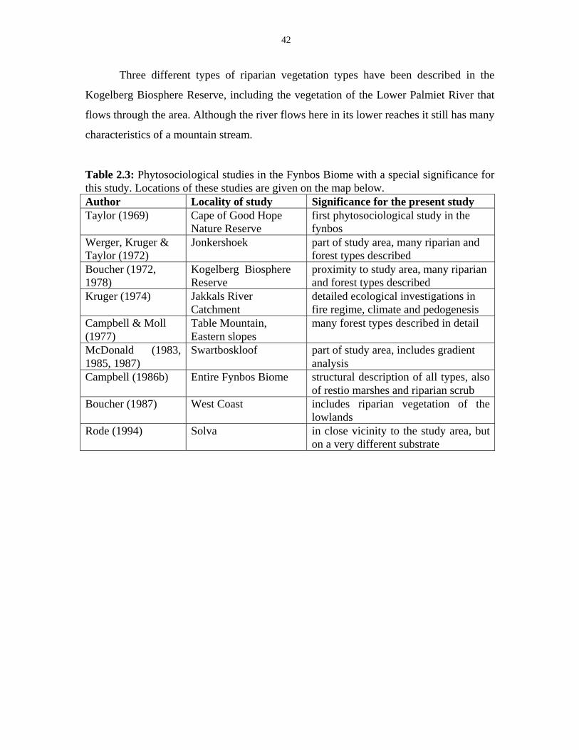
42
Three different types of riparian vegetation types have been described in the
Kogelberg Biosphere Reserve, including the vegetation of the Lower Palmiet River that
flows through the area. Although the river flows here in its lower reaches it still has many
characteristics of a mountain stream.
Table 2.3: Phytosociological studies in the Fynbos Biome with a special significance for this study. Locations of these studies are given on the map below. Author Locality of study Significance for the present study Taylor (1969) Cape of Good Hope
Nature Reserve first phytosociological study in the fynbos
Werger, Kruger & Taylor (1972)
Jonkershoek part of study area, many riparian and forest types described
Boucher (1972, 1978)
Kogelberg Biosphere Reserve
proximity to study area, many riparian and forest types described
Kruger (1974) Jakkals River Catchment
detailed ecological investigations in fire regime, climate and pedogenesis
Campbell & Moll (1977)
Table Mountain, Eastern slopes
many forest types described in detail
McDonald (1983, 1985, 1987)
Swartboskloof part of study area, includes gradient analysis
Campbell (1986b) Entire Fynbos Biome structural description of all types, also of restio marshes and riparian scrub
Boucher (1987) West Coast includes riparian vegetation of the lowlands
Rode (1994) Solva in close vicinity to the study area, but on a very different substrate
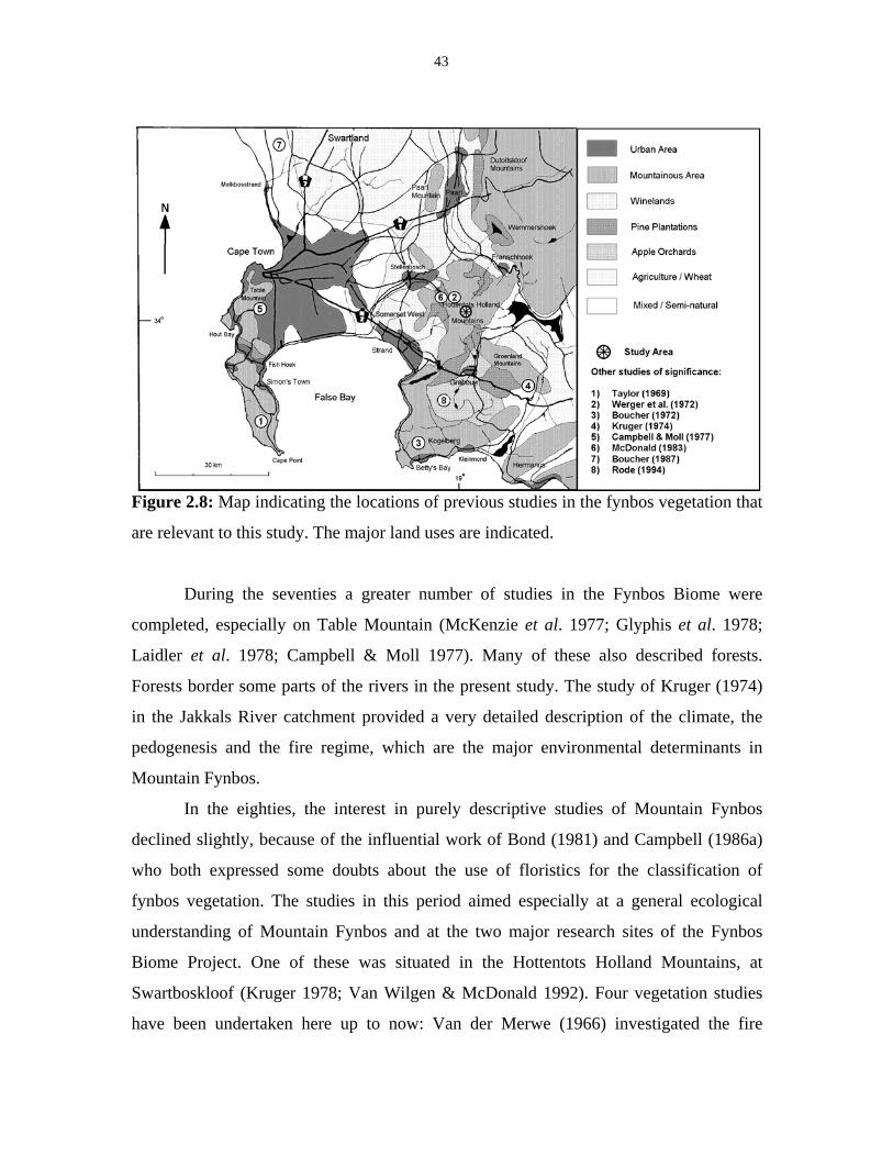
43
Figure 2.8: Map indicating the locations of previous studies in the fynbos vegetation that
are relevant to this study. The major land uses are indicated.
During the seventies a greater number of studies in the Fynbos Biome were
completed, especially on Table Mountain (McKenzie et al. 1977; Glyphis et al. 1978;
Laidler et al. 1978; Campbell & Moll 1977). Many of these also described forests.
Forests border some parts of the rivers in the present study. The study of Kruger (1974)
in the Jakkals River catchment provided a very detailed description of the climate, the
pedogenesis and the fire regime, which are the major environmental determinants in
Mountain Fynbos.
In the eighties, the interest in purely descriptive studies of Mountain Fynbos
declined slightly, because of the influential work of Bond (1981) and Campbell (1986a)
who both expressed some doubts about the use of floristics for the classification of
fynbos vegetation. The studies in this period aimed especially at a general ecological
understanding of Mountain Fynbos and at the two major research sites of the Fynbos
Biome Project. One of these was situated in the Hottentots Holland Mountains, at
Swartboskloof (Kruger 1978; Van Wilgen & McDonald 1992). Four vegetation studies
have been undertaken here up to now: Van der Merwe (1966) investigated the fire
44
response of the vegetation. Werger et al. (1972) introduced the Braun-Blanquet method
to the Fynbos Biome and presented the first phytosociological description of some
selected vegetation units. Van Wilgen (1981) mainly investigated the effects of fire while
McDonald (1983, 1985) undertook a second, more complete, phytosociological survey of
the area. Fry (1987) provided a detailed account of soils found in the valley and related
that to the vegetation units described by McDonald (1983). In this period also
phytosociological studies that included gradient analysis were carried out (e.g. McDonald
1987).
In the nineties the interest in ‘classical’ descriptive studies according to the
Braun-Blanquet method in Mountain Fynbos increased again. Some studies from this
period are the ones by McDonald (1993a-c) from the Langeberg and Taylor (1996) from
the Cedarberg.
2.7 Riverine ecosystems
With higher water demands for an increasing South African population, the situation has
already been reached where nearly every medium-sized river in the country is impounded
in at least one place. The ecological consequences of these pressures on the vulnerable
riverine ecosystems has received more attention since the end of the eighties (Ferrar et al.
1988). The more intensive river research since then is aimed at assessing the amount of
water in a river that can be utilized by the human population, while the ecosystem itself is
also seen as a ‘competing user’ or later even as the resource base without which
sustainable use is not possible (King et al. 2000).
Riverine ecosystems are very fragile systems, because they are dependent on the
condition of their entire catchment. If there is one point source of pollution somewhere in
a river catchment, this will be evident everywhere downstream from that point. And yet,
riverine ecosystems have the ability of self-purification and every aquatic disturbance has
a downstream recovery distance (Ward & Stanford 1979). With the present population
pressure in South Africa, however, it is impossible to conserve rivers entirely in their
natural state and some kind of compromise fitting the demands of the people has to be
found (Ferrar et al. 1988). Nowadays, Environmental Flow Assessments for rivers are
45
conducted in a holistic manner before their water resources are exploited further (King et
al. 2000).
2.7.1 General river ecology
A river is an essential part of the hydrological cycle. In hydrology one cannot separate a
river from its catchment area. The catchment includes a very complicated network of
streams, gullies, swamps, seepages and rivers, together with all the bodies of water that
move underground. This network of water bodies can only persist in areas where
precipitation exceeds evaporation. Water will start flowing superficially when the soil is
completely saturated. When the water flows it first collects into little rills. These join
together to form gullies. These flow together into the first order rivers that join again to
form second order rivers and so on. In this way a branching river system is formed
(Hynes 1970).
Along its course a river can be divided into three longitudinal zones: The
Mountain Stream Zone, where the erosion exceeds the sediment accumulation, the
Foothill Zone where erosion and accumulation are more or less in equilibrium, and the
Coastal Plain River Zone where accumulation exceeds erosion (Davies & Day 1998).
This longitudinal zonation is merely for descriptive purposes, but in reality a river rarely
shows sharp boundaries along its longitudinal gradient (Hynes 1970). In an ‘ideal river’ a
graph of the altitude against the distance from the coast would show a perfect concave
curve with the mountain river zone showing the steepest angle which will gradually
decrease on its course towards the coast. In reality there are alterations in this pattern due
to geological heterogeneity (Davies & Day 1998).
The channel morphology is determined by a number of factors and differs along
the different reaches. Riffles and pools alternate, riffles in the shallow places and pools in
the deeper places. Riffles tend to occur at regular intervals, in places where larger
boulders are clustered. They do not occur on sandy riverbeds because they are correlated
with a diversity of particle sizes. The deeper part of the river, or the main stream, has a
natural tendency to swing from one side to the other thus, especially in the lower reaches,
meandering channels are found (Hynes 1970).
46
Lateral riparian zones form the interface between the riverine ecosystem and the
surrounding uplands. They add an extra dimension to the riverine ecosystem and the river
receives many nutrients from the soil in the riparian zone (Naiman & Décamps 1997).
The river creates many different habitats here during floods and it is one of the most
dynamic ecosystems as it also suffers from the upland disturbances. These disturbances
result in a high species diversity in riparian zones worldwide. Many authors claim that
maximum biodiversity will occur in places that experience an intermediate level of
natural disturbances, which applies well to rivers (Ward & Stanford 1983; Gregory et al.
1991).
2.7.1.1 Mountain streams
First, the situation in mountain headwater streams will be described. A typical mountain
stream is cool, clear and fast flowing. It is the flow of water that dictates what remains in
the channel and what is removed. The riverbed is mainly covered by bedrock or boulders,
which results in rapid flow and highly oxygenated water. The land that the river drains is
usually very rocky with very little loose soil, so the sediment load is low, while the
carrying capacity is high. Mountains that consist of hard rocks, that weather slowly, will
have water flowing through them that is low in nutrients. This, together with the fast
flow, as well as the shading of the edges, will make the mountain stream a harsh climate
for plants and animals to live in (Davies & Day 1998).
In the Western Cape, the headwaters of the rivers are oligotrophic which reflects
the low level of nutrients in the soil. There is also a low value for Total Dissolved Solids
and a low pH (although there are some variations in pH). Altogether, this results in a high
potability. Plants that grow in the riverbed extend their roots into the soil with difficulty
because of the eroding nature of the stream. They must have strong root systems to
withstand high flow rates. The main food supply in mountain streams will be
allochtonous plant material: leaves, bark, twigs and fruits of the plants lining the rivers
edge. Mountain streams belong to those few ecosystems that rely entirely on an external
food source (Hynes 1970). The decomposing bacteria and fungi contribute to the total
food resource. This results in the ratio P:R < 1, that means that the production (P) is less
47
than the respiration (R). Animals that live in the mountain streams will have to adapt to
this food source and can be classified as grazers, collectors, scrapers or shredders,
depending on the way they take their food (Davies & Day 1998).
Despite the many difficulties that organisms have to cope with, many different
microhabitats can be found in the mountain streams, on the banks as well as in the
aquatic environment. Some of these are pools (deep places with low to zero velocity and
smooth flow), runs (shallow to deep places with smooth flow and moderate velocities),
riffles (high-velocity areas with turbulent flow and broken water surfaces) and cascades
(places with free-falling water over bedrock and boulders in step-like arrangements). The
microhabitats will change as the water level fluctuates. During a high flood, for example,
riffles and pools turn into runs and the cascades can disappear completely (Davies & Day
1998).
During spates or droughts many animals can seek shelter in the hyporheos (the
riverbed itself) where they can dig down into the substrate to a depth of up to one meter.
This is an often overlooked part of the riverine ecosystem. It plays a major role, though,
in the cycling of nutrients in the river ecosystem. It appears that the river itself is only
part of a much bigger waterbody that extends underground both laterally and basally
(Day et al. 1986; Davies & Day 1998).
A distinct feature of many rivers in the Western Cape, especially those on
seaward facing slopes and those in the east, is the brown coloration of the water. It must
be noted that this brown-ness increases after heavy rains. The darker colour of the water
is often correlated to the acidity and King & Day (1979) assume that the cause of it is the
presence of ‘humic acids’ in the water. The reason why some waters are browner than
others, might be the extensive seepages at the mountain tops (own observation). This will
also explain the sudden dark coloration of river water after heavy rains. Another cause of
the dark waters that has been suggested is that the detritus of the sclerophyllous ericoid
fynbos vegetation is rich in tannins that give the water a dark colour. The litter of
sclerophyllous vegetation does not break down as easily as the detritus of forest trees, so
the colour of the tannins remains in the water (Stewart & Davies 1990). When the water
in the rivers continues its course in the Foothill Zone, the TDS (total dissolved solids)
48
and turbidity will increase, resulting in a better-buffered system that is more alkaline and
less brown (King & Day 1979).
2.7.1.2 Lower rivers
Although they do not form part of this study, a short introduction to the lower rivers and
the estuaries will be given to provide a more complete scenario of a river ecosystem.
In the Foothill Zone the river size increases as the catchment size increases. The
slope here is more gentle so the current speed decreases. As the riverbed widens more
sunlight reaches the water, hence water temperatures increase and more algae grow in the
river. More soil is washed into the river from the surroundings so that the river carries
more suspended material. Both living organisms and the erosion of soil result in water
that is less clear than in the headwaters (Davies & Day 1998).
More algae occur in the middle reaches of the river and the production of organic
matter in the water increases. The P:R-ratio (Production / Respiration) is greater than 1.
The invertebrates that feed on the algae still have the same adaptations to those in the
mountain stream, because the stream velocity is still high and the riverbed stony. They
tend to be different species, though. They also have a more distinct life-cycle, because
temperatures in the middle reaches show more variation throughout the year (Davies &
Day 1998).
As the river continues its way through the lowlands it enters the coastal plain
where the slope and the stream velocity decrease more. The sediment load of the river is
deposited as the slow-moving water cannot carry it any longer. The finer particles are
deposited close to the sea where velocities are minimal. The water in the lower reaches is
the richest in nutrients as it carries all the nutrients leached from the higher reaches. The
riparian environment is ideal for the development of dense stands of emergent plants such
as reeds or bulrushes (Davies & Day 1998).
There are many variations to the pattern described here for mountain streams,
foothill zones and lower rivers. Some rivers in the Western Cape, such as the Palmiet and
Rooiels Rivers, enter the sea directly from the mountains. These rivers do not have a
lower river zone at all. In other cases, a river can be ‘rejuvenated’ when it crosses an
49
escarpment, for example like the Orange River at the Augrabies Falls or the Zambezi at
Victoria Falls and later at Cahora Bassa (Davies & Day 1998).
2.7.1.3 Estuaries
The estuary of a river is the most vulnerable part of a river ecosystem, because it is
influenced by all the anthropogenic activities upstream. Coastal ecosystems benefit a lot
from nutrient-rich sediments in the sea and estuaries are often good fishing grounds.
Estuaries gain particulate matter from both the river and the sea and are among the most
productive ecosystems in the world. Many of the South African estuaries are closed for a
part of the tidal cycle. A detailed description of South African estuaries is provided by
Day (1981) and by O’Callaghan (1993).
2.7.2 The river catchment
Many processes taking place in a river are catchment-related and these will be discussed
in this section. The catchment or subcatchment of a river or section of a river is subject to
a specific climate and has a specific geological substrate. All of these characteristics will
reflect in the riverine ecosystem, the runoff and the water quality (Boucher & Marais
1993).
Precipitation that falls into a catchment will ∠ if it is not lost through
evapotranspiration ∠ flow downhill, either as surface or as ground water. The movement
of the subsurface flow is extremely complex and has an important effect on the water
chemistry. After a storm many of the subsurface flows might form small rivers and a
dense network of small temporary streams is created (Crabtree & Trudgill 1985).
Instead of forming a fixed network of river channels, streamflow is generated in a
dynamic, expanding or shrinking source area. This is summarized in the Variable Source
Area Concept (Hewlett 1961; Hewlett & Hibbert 1967). After water has infiltrated into
the soil, the depth and porosity of the soil help determine whether the water remains in
the soil or emerges as streamflow. Some water might be stored in the soil for years, while
the rivers only depend on water supply from another nearby source. Wet periods might
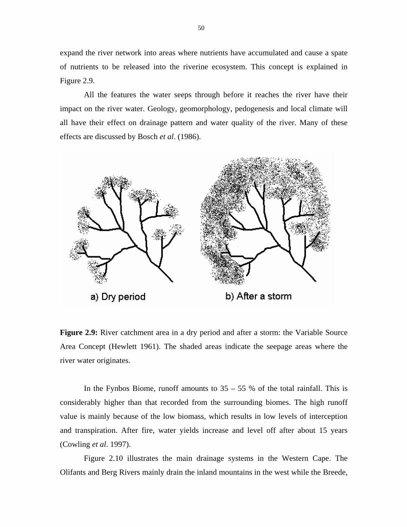
50
expand the river network into areas where nutrients have accumulated and cause a spate
of nutrients to be released into the riverine ecosystem. This concept is explained in
Figure 2.9.
All the features the water seeps through before it reaches the river have their
impact on the river water. Geology, geomorphology, pedogenesis and local climate will
all have their effect on drainage pattern and water quality of the river. Many of these
effects are discussed by Bosch et al. (1986).
Figure 2.9: River catchment area in a dry period and after a storm: the Variable Source
Area Concept (Hewlett 1961). The shaded areas indicate the seepage areas where the
river water originates.
In the Fynbos Biome, runoff amounts to 35 – 55 % of the total rainfall. This is
considerably higher than that recorded from the surrounding biomes. The high runoff
value is mainly because of the low biomass, which results in low levels of interception
and transpiration. After fire, water yields increase and level off after about 15 years
(Cowling et al. 1997).
Figure 2.10 illustrates the main drainage systems in the Western Cape. The
Olifants and Berg Rivers mainly drain the inland mountains in the west while the Breede,
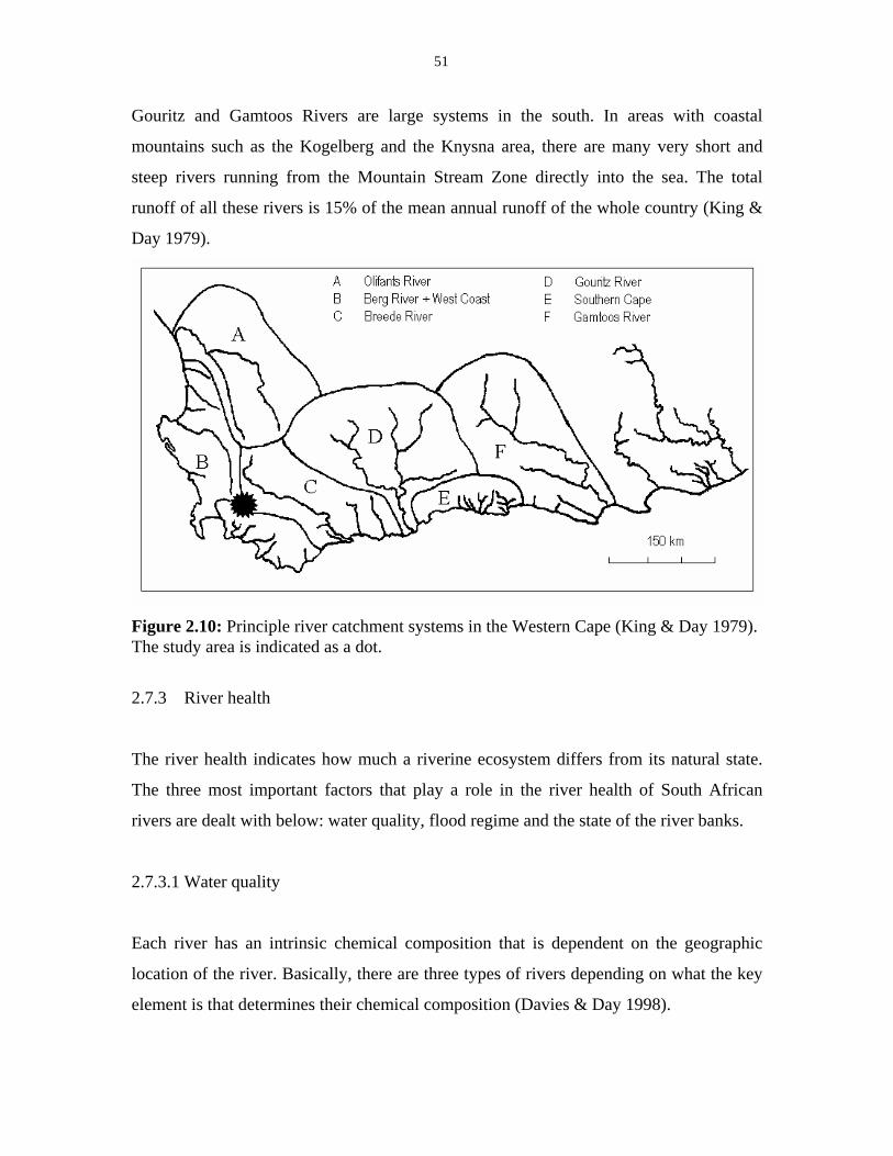
51
Gouritz and Gamtoos Rivers are large systems in the south. In areas with coastal
mountains such as the Kogelberg and the Knysna area, there are many very short and
steep rivers running from the Mountain Stream Zone directly into the sea. The total
runoff of all these rivers is 15% of the mean annual runoff of the whole country (King &
Day 1979).
Figure 2.10: Principle river catchment systems in the Western Cape (King & Day 1979). The study area is indicated as a dot.
2.7.3 River health
The river health indicates how much a riverine ecosystem differs from its natural state.
The three most important factors that play a role in the river health of South African
rivers are dealt with below: water quality, flood regime and the state of the river banks.
2.7.3.1 Water quality
Each river has an intrinsic chemical composition that is dependent on the geographic
location of the river. Basically, there are three types of rivers depending on what the key
element is that determines their chemical composition (Davies & Day 1998).

52
- Some geological formations weather readily and many minerals are leached into
the water. The mountains of Lesotho with their igneous basalt rocks are a good
example. The minerals in the water are dominated by calcium, magnesium and
bicarbonate. Their pH is slighly above 7. These waters are said to be ‘rock-
dominated’ (Davies & Day, 1998).
- On the other hand, there are rock formations, like sandstones, that consist of old
sediments that are highly leached already and release few minerals into the water
on weathering. This is the situation in most of the Fynbos Biome. The minerals in
water from this type of substrate are dominated by sodium and chloride, which
are the dominant elements in rainwater. These waters are said to be ‘rain-
dominated’ (Davies & Day, 1998).
- Rain- or rock-dominated rivers can flow through arid areas in their lower reaches.
Much water evaporates there and the concentration of salts in the water increases.
These waters are said to be ‘evaporation-dominated’ (Davies & Day, 1998).
Human activities in the catchment area can influence the natural chemical composition of
the water and affect water quality. Overall water quality can be measured as a set of
physical attributes and chemical constituents. A description of some of these is given in
Appendix B.
2.7.3.2 The flood regime
The hydrology of a river is important for many of the ecological processes in the river,
such as maintenance of the river channel and of the wet biotopes. The ecological flow
requirement of a system is defined as ‘that flow which is critical for the maintenance of
the essential ecological functioning of the river’ (O’Keeffe et al. 1989).
Flow can be regulated and decreased by various human impacts such as
impoundment, inter-basin-transfer or water abstraction. All these will affect the natural
flow regime of the river. There are two aspects that determine the ecological flow: the
base-flow and the flood regime.
The base-flow is the flow that is always present in the river. Base-flows keep
hydraulic conditions suitable for the invertebrate life in many biotopes and function as
53
refuges for fish (Davies et al. 1993). If base-flows are reduced there will be a change in
the environmental conditions of the river. The assumption of Prewitt & Carlson (1980) is
that this change is seldom linear, but usually exponential or asymptotic. This means that
the river can deal with a slight modification, but as soon as the flow reduction reaches a
certain critical level, it will have severe effects. This point is known as the inflection
point. If the water level in the river becomes lower, initially it will only mean a slight
reduction in the benthic habitat. As soon as the stony bed is reached, the entire benthic
habitat is lost and serious changes take place in the riverbed (O’Keeffe et al. 1989).
The flood regime or variability in flow is at least as important for the basic
ecological functioning of the river as the base-flow. Floods keep the river channel in
shape and heavy floods can modify the river channel. They are also important for fish
breeding and can flush poor quality water from pools. Rivers in South Africa are
characterised by a seasonal flow pattern. The predictable seasonal changes in flow have
resulted in specialized aquatic communities, adapted to both very fast flowing and almost
stagnant waters. In rivers that experience severe spates, serious droughts or unpredictable
floods only an impoverished faunal community will persevere. In the Western Cape big
floods will only occur in the winter months, but summer floods (also called freshets) have
an equally important role for river functioning (Department of Water Affairs and Forestry
1994).
Hynes (1970) mentioned that floods that almost fill the river channel are the ones
that maintain the channel form. This level is called the bankfull discharge and is reached,
on average, about every 1.5 years. Bigger floods have longer occurrence intervals and
can be expressed as a factor times the bankfull discharge.
The characteristics of individual flood events is best described by the hydrograph
shape. The hydrograph is the measured discharge by a water level recorder, plotted over
time, starting with the beginning of the rainstorm. The volume of the flood event
determines whether there will also be a flood downstream (Bosch et al. 1986).
The different habitats on the riverbanks are all affected by the different types of
floods. The flood regime creates a diversity of temporary wet habitats on the riverbanks,
which are discussed below.
54
2.7.3.3 The riverbank
A cross-section through a riverbed shows different habitats, which are affected
differently by different flow levels. The conditions in these habitats are determined by the
frequency of flooding and by the inundation period. The geomorphology determines how
wide the lateral riparian zone is. Where slopes are flat and soils have a high water
holding capacity a floodplain will develop and create a very wide riparian zone. Usually,
the development of the riparian zone becomes more significant in mature rivers of a high
stream order. Exceptions are the riparian forests and the source-area seepages, which can
also be very wide (Rogers & Van der Zel 1989).
The riparian zone should be distinguished from the phreatic zone, an area
recognised by forest hydrologists to describe the area adjacent to watercourses in which
trees have constant access to freely available water (Bosch & Versfeld 1982).
The riparian zone is an interface between the terrestrial and the aquatic ecosystem
and it has considerable influence on the aquatic ecosystem. Most of the nutrient inputs
into the river ecosystem come from the riparian zone (Naiman & Décamps 1997) and the
riparian vegetation also serves as an allochtonous food resource for aquatic organisms
(King 1981; Stewart & Davies 1990). Riparian ecosystems are extremely complex and
are rich in ecological processes. Flooding influences the terrestrial ecosystems while
nutrient inputs and subsurface flows have a large impact on the aquatic ecosystems
(Gregory et al. 1991; Naiman & Décamps 1997).
The first author who described the influence of the river on the vegetation
growing on its banks was Illichevsky (1933). Thirty years later, Kopecky (1969) dealt
with the vegetation in the riparian zone in detail. He classified European watercourses
according to the following criteria:
- the vertical division of the river banks into riparian and subriparian zones.
- the range over which the water level fluctuates.
- the intensity of wave action or speed of flow.
Two fundamental bank types are distinguished by him, based on the amplitude of
fluctuations of the water level. The stenosaleutic type is characteristic for small
watercourses and for rivers with wide beds and very flat banks. The difference between
55
maximum and minimum yearly water levels does not exceed 0.60 m. In general,
riverbanks in the mountain stream zone belong to this type. The eurysaleutic type, in
which the water level fluctuates more than one meter, is found more in the lower parts of
rivers (Kopecky 1969). The distinction between constricted and unconstricted reaches, as
mentioned by Gregory et al. (1991), shows much similarities with this subdivision.
The stenosaleutic type of riverbanks can be divided into at most four different
ecotopes according to the time spent under water. The submerse ecotope is permanently
under water. The demerse ecotope is mostly under water; it is exposed only shortly
during the dry season. In smaller rivers this ecotope will barely be recognizable. The
semimerse ecotope regularly dries out and is then wetted again during a small flood. This
is the lower zone of the riparian zone, which we will later refer to as the Wet Bank.
Finally, the emerse ecotope is the area of the riparian zone that will only be inundated
during high floods. In every ecotope different vegetation types are recognizable. In the
eurysaleutic type, where oscillations of the water level are much higher, the differences
are much more distinct. Here the semimerse ecotope can be subdivided into the
subsemimerse and the suprasemimerse ecotope (Kopecky 1969).
The riverbanks can be divided into lentic and lotic parts when they are flooded. In
the lentic parts the water movement is decreased to a minimum and the silt load will be
deposited in these places (Kopecky 1969).
Since Kopecky (1969) many authors have proposed different classifications of
riparian habitats. Many kept it very simple, such as Hupp & Osterkamp (1985) and
Gregory et al. (1991). Different classifications apply to rivers with a different
geomorphology, for example the classification by Menges & Waller (1983) applies to
rivers with floodplains, while Dixon & Johnson (1999) deal with vegetation on steep
river banks. Menges & Waller (1983) base their subdivision on the life strategies of the
plants growing in each zone while most other authors base the subdivision on the
ecological processes that take place. This is a problem because different reaches are
dominated by different processes. In the higher reaches erosion dominates, while in the
lower reaches deposition is more important (Davies & Day 1998). There are also the
different influences that floods can have on the lateral zones. There are reaches that are
mainly affected by the inundation of floodwater (Kopecky 1969; Menges & Waller 1983;
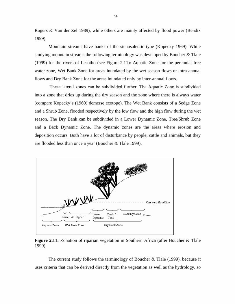
56
Rogers & Van der Zel 1989), while others are mainly affected by flood power (Bendix
1999).
Mountain streams have banks of the stenosaleutic type (Kopecky 1969). While
studying mountain streams the following terminology was developed by Boucher & Tlale
(1999) for the rivers of Lesotho (see Figure 2.11): Aquatic Zone for the perennial free
water zone, Wet Bank Zone for areas inundated by the wet season flows or intra-annual
flows and Dry Bank Zone for the areas inundated only by inter-annual flows.
These lateral zones can be subdivided further. The Aquatic Zone is subdivided
into a zone that dries up during the dry season and the zone where there is always water
(compare Kopecky’s (1969) demerse ecotope). The Wet Bank consists of a Sedge Zone
and a Shrub Zone, flooded respectively by the low flow and the high flow during the wet
season. The Dry Bank can be subdivided in a Lower Dynamic Zone, Tree/Shrub Zone
and a Back Dynamic Zone. The dynamic zones are the areas where erosion and
deposition occurs. Both have a lot of disturbance by people, cattle and animals, but they
are flooded less than once a year (Boucher & Tlale 1999).
Figure 2.11: Zonation of riparian vegetation in Southern Africa (after Boucher & Tlale 1999).
The current study follows the terminology of Boucher & Tlale (1999), because it
uses criteria that can be derived directly from the vegetation as well as the hydrology, so
57
it is quite practical in its use. However, the streams in this study are in higher reaches
than the ones studied in Lesotho and fewer zones can be recognized because zones tend
to concatenate on each other.
The riparian vegetation has the following functions in a riverine ecosystem:
- control of water velocity, slowing and spreading flood waters;
- control of erosion of riverbeds and banks;
- water retention, thus increasing evapotranspiration and groundwater recharge;
- increased deposition rate of organic and inorganic suspended solids;
- nutrient retention and sink for pollutants;
- enhancement of biotic diversity through heterogeneity of habitats.
For these reasons laws protecting the riparian vegetation against afforestation have been
in existence for a long time in South Africa (Rogers & Van der Zel 1989). Nowadays, the
importance of the riparian zone for river management is widely recognized and the study
of riparian systems is included in many environmental impact assessments for rivers
(MacKenzie et al. 1999; King et al. 2000; Ward & Wiens 2001; Zalewski et al. 2001).
It is not only that the flood in the river influences vegetation growth; the opposite
is also true. The processes of erosion and accumulation mutually depend on each other
and are influenced by the riparian vegetation. During a high flood, the vegetation on the
riverbank slows down the current in the river, thereby stimulating the deposition of
sediments. However, if the current is slowed down in one part of the river, the current
will be accelerated in another part, which would then in turn stimulate the erosion
process. In this way riparian vegetation exerts considerable influence on channel
morphology and thus on floods. It is also the vegetation that determines where sediments
in the stream accumulate; this accumulation will also slow down the current (Kopecky
1963). The density of the riparian vegetation has a big impact on the bed roughness of the
river and thus on the flood discharges to be expected in a particular reach (Gordon et al.
1992; McKenney et al. 1995).
Plants growing next to a river channel have strategies to cope with the differences
in depth of the water table and inundation (Menges & Waller 1983). Hydrologically,
riverbanks can be divided into two types: the floodplain type and the bank-storage type.
In the floodplain type, inundation (permanent or periodic) is the main determinant of
58
structure and functioning of the ecosystem. This type is usually only found in the lower
reaches, but it can also occur in high altitude seepages. In the bank-storage type
inundation is absent or infrequent and the groundwater level is the major determinant of
ecological processes (Rogers & Van der Zel 1989).
Both situations imply stress-factors for the plants. The main stresses that occur in
a situation of bank-storage are a result of either anaerobic conditions when the soil is
saturated, or water stress that occurs during the dry season or droughts. During floods the
stress of extended periods of inundation results in anaerobic conditions in the soil. There
might be toxic effects of certain nutrients during anaerobic conditions. There are many
different strategies to cope with these stresses (Pezeshki 1994). Turbulent conditions
during floods cause destruction by uprooting plants, which results in a decrease in their
density. The juvenile stages are especially sensitive, because they do not have extensive
root systems. However, this also brings new opportunities for the establishment of
seedlings of the same or other species (Rogers & Van der Zel 1989).
2.7.3.4 Anthropogenic influences
Human interference can upset the natural situation described in paragraphs 2.7.3.1 to
2.7.3.3. Water quality is affected by pollution, the flood regime can be altered by dams
and weirs and the riparian vegetation can become invaded by exotic species. Methods
have been developed to make an assessment of the conservation status of riverine
ecosystems in South Africa, but no standardized methods exist. In the Western Cape, the
method developed by Kleynhans et al. (1988) is applied most often.
Pollution
The word pollution here refers to any alteration of the natural state of the water quality,
mostly caused by humans. The most visible forms of pollution, such as cans and bottles
near the river, often draw most attention, but this is not always the worst form of
pollution. Many toxic substances can be spilt into the river system that are not readily
visible but may have disastrous effects. Even many naturally occurring substances can
59
become pollutants, when their concentrations increase until they reach toxic levels.
Detailed accounts of pollution are given by Hynes (1963) and Davies & Day (1998).
Dams and weirs
In a country like South Africa, with an unpredictable rainfall and with very few natural
lakes, reservoirs are needed to ensure that there is sufficient water available for human
consumption and agriculture, even during periods of drought. This is why nearly every
major river in South Africa is impounded in at least one place. However, dams are a
major threat to the riverine ecosystems. A general account of the influence of dams on
water quality downstream, fisheries, floodplains and estuaries can be found in Ward &
Davies (1984).
Locally, following construction of an impoundment, the riverine ecosystem
changes completely as the river turns into a lake. After a dam is constructed the
impounded water enters an unstable phase in which environmental factors fluctuate
strongly. In this phase many minerals leach from the inundated soils, some of which may
be toxic. They change the water chemistry substantially and many aquatic organisms may
become extinct or be replaced by others (Davies & Day 1998).
The flow regime of a river below a dam is influenced considerably by the
management of water discharge from the dam. Naturally, river flows can be quite
unpredictable. Regulated rivers, though, have few small floods and less extreme events
such as big floods or complete droughts, and the variation in flows will become more
predictable and less variable. This will have a direct influence on organisms living in the
stream and the riparian habitat. Things that might happen when dams are not well
managed, are loss of biodiversity, collapse of estuarine fisheries, loss of riparian
vegetation and more severe floods (Ward & Davies 1984; Davies et al. 1993).
A reservoir, therefore, has two immediate influences on the river downstream: it
affects its water quality and its flow regime. Ward & Stanford (1979) deal with both in
detail and show that the disturbance caused by a dam will diminish at some point
downstream. The reset distance to this point is determined by the level of disturbance and
of the reach in which the dam was built. In general, dams in the upper and lower reaches
are more favourable than those in the middle reaches because the reset distances are the
60
smallest here (Ward & Stanford 1983; Ward & Davies 1984). Drier conditions due to
lower flood levels place the riparian vegetation under stress. This increases the potential
for invasion by exotic plants (Macdonald & Richardson 1986).
Exotic plants
The above-mentioned anthropogenic influences will mainly affect the lower reaches of a
river. The only disturbance likely to occur in both the upper and lower reaches is the
threat of alien invasive vegetation. Few of the herbaceous invasive species have had a
serious impact in the mountains; the majority of the troublesome species are woody
shrubs (Macdonald & Richardson 1986). This also implies that many of the ecological
processes in the vegetation change after it becomes infested with alien species. Species
diversity will decrease because understorey shrubs are not adapted to shady conditions
and fuel loads of the vegetation will increase (Versfeld & Van Wilgen 1986).
The Fynbos Biome is extremely sensitive to invasion by exotic plants. Many
species that have been introduced into the whole of South Africa are only invasive in the
Fynbos Biome. Invasive species need an effective dispersal agent, a suitable habitat and a
competitive advantage over the indigenous vegetation in order to establish themselves.
Even if they can grow vigorously, climatic conditions may prohibit seed setting or
dispersal (Kruger et al. 1986). Yet, some species like Pinus pinaster and Hakea sericea
are able to invade undisturbed Mountain Fynbos communities. The phenomenon that
alien species invade indigenous communities without a disturbance having taken place is
very rare throughout the rest of the world (Richardson et al. 1992).
Rivers form a specific habitat for the dispersal of another group of invasive exotic
plants, the Australian Acacia species, that are mainly dispersed by ants, although some
species may be dispersed by birds and by water (see below). Riparian habitats are
invaded by a number of species, among them Acacia longifolia, A. mearnsii, A. saligna,
Paraserianthus lophantha and Sesbania punicea. The flooding of the riparian zones may
scarify the hardcoated seeds of the acacias and stimulate their growth here. They are also
very well adapted to the fire regime in the Cape, because their natural habitat in Australia
is also very fire-prone (Richardson et al. 1992).
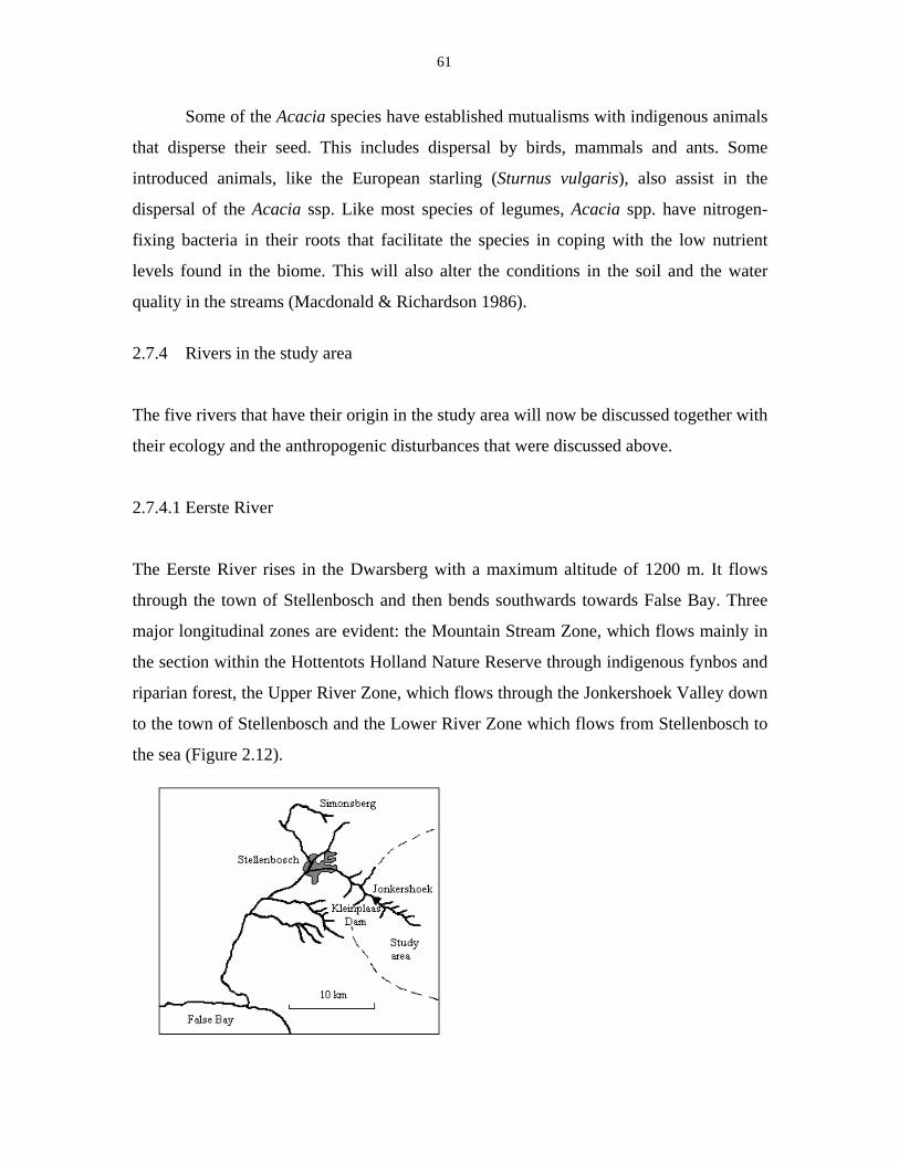
61
Some of the Acacia species have established mutualisms with indigenous animals
that disperse their seed. This includes dispersal by birds, mammals and ants. Some
introduced animals, like the European starling (Sturnus vulgaris), also assist in the
dispersal of the Acacia ssp. Like most species of legumes, Acacia spp. have nitrogen-
fixing bacteria in their roots that facilitate the species in coping with the low nutrient
levels found in the biome. This will also alter the conditions in the soil and the water
quality in the streams (Macdonald & Richardson 1986).
2.7.4 Rivers in the study area
The five rivers that have their origin in the study area will now be discussed together with
their ecology and the anthropogenic disturbances that were discussed above.
2.7.4.1 Eerste River
The Eerste River rises in the Dwarsberg with a maximum altitude of 1200 m. It flows
through the town of Stellenbosch and then bends southwards towards False Bay. Three
major longitudinal zones are evident: the Mountain Stream Zone, which flows mainly in
the section within the Hottentots Holland Nature Reserve through indigenous fynbos and
riparian forest, the Upper River Zone, which flows through the Jonkershoek Valley down
to the town of Stellenbosch and the Lower River Zone which flows from Stellenbosch to
the sea (Figure 2.12).
62
Figure 2.12: The Eerste River catchment area.
Parts of the upper reaches of the river have been studied in some detail, inter alia
the aquatic animals by King (1981) and vegetation by McDonald (1985) and Van Wilgen
& McDonald (1992) This last study was done in the Swartboskloof subcatchment, which
was one of the intensive study sites for the Fynbos Biome Project.
The study by King (1982) on the invertebrate fauna of the Eerste River provides
some information about the physical environment of the river. Discharge in the river is
biggest in winter with major spates in May and July, and lowest between December and
March. Water temperature in winter is low in all reaches of the river (between 10°C and
14°C), but shows increase downstream during summer. Variations in pH are small
between the different seasons, but water tends to be more alkaline in the lower than in the
upper reaches. The amount of nutrients and the buffering capacity increase downstream
and are generally higher in summer than in winter.
In the higher reaches of this river, Table Mountain Group sediments are
dominant, but lower down in the valleys granites of the Cape Granite Suite and alluvial
sediments dominate. Waters draining such areas are naturally pure and have a low buffer
capacity.
The Kleinplaas Dam, just below Jonkershoek on the Eerste River (built in 1981)
holds water from the Riviersonderend-Berg-Eerste River Government Water Scheme
through a series of interconnecting tunnels and an Interbasin Transfer Scheme. The
advantage of this system is that water can be released from the Theewaterskloof Dam
when water demand exceeds availability in the Eerste River Valley itself. Therefore the
Kleinplaas Dam is said to be a balancing and diversion structure. Petitjean (1987)
estimates that 48% of the run-off of the river is abstracted to other catchments. The
compensation flows from Theewaterskloof Dam are allocated entirely to the water users
such as farmers and industries. This results in a water shortage between the Kleinplaas
Dam and Stellenbosch during the summer months (Petitjean 1987).
The dam is also used as an experimental trout breeding station administered by
the University of Stellenbosch. Investigations are under way to assess the feasibility of
63
building a second dam higher up the river than the Kleinplaas Dam and for a third along
the lower Eerste River at Faure (Brown & Dallas 1995).
Downstream from the nature reserve the river flows through agricultural land
(mainly vineyards) and is more often accompanied by exotic trees such as oaks (Quercus
robur), poplars (Populus canescens) and gum trees (Eucalyptus spp.). The indigenous
vegetation that remains, mainly consists of Metrosideros angustifolia and Brabejum
stellatifolium (Brown & Dallas 1995).
In this zone and below, water abstraction takes place to such an extent that parts
of the river cease flowing in summer. This has serious consequences for the riverine
ecosystem. Firstly, decrease in flow means an alteration of the physical habitat. This has
a big influence on the life cycles of the aquatic biota, for example on the passage of fish.
Secondly, reduced discharge means that the pollution that enters the river in the lower
parts is not diluted (Brown & Dallas 1995).
In the Lower River Zone, the river is heavily polluted, especially downstream
from the confluence with the Plankenbrug and Veldwachters Rivers. Petitjean (1987)
states that this has already been the case for a fairly long time, ever since the sixties. The
two tributaries of the Eerste River in Stellenbosch have a deleterious effect on the river.
The Plankenbrug River rises in the Simonsberg and runs through an agricultural area.
The Veldwachters River receives effluent from the Stellenbosch Municipality Sewage
Works (SMSW). Although the Eerste River is a Special Standards River, the SMSW has
been granted a license to release its General Standard effluent into the Veldwachters
River. In summer, 95% of the flow in the Veldwachters River is sewage effluent
(Petitjean 1987; Brown & Dallas 1995).
The Eerste River has a high conservation status in its upper reaches, and a low
conservation status in its lower reaches. This is a pattern that occurs in many of the rivers
in the region. The conservation importance of the river is determined by its proximity to
the town of Stellenbosch and its recreational use in that area (Brown & Dallas 1995).
2.7.4.2 Berg River
64
Nearly the whole northern section of the Hottentots Holland Nature Reserve is drained by
the Berg River (Figure 2.13), with the exception of the area around the Franschhoek Pass,
which is drained by the Riviersonderend River. The catchment consists of three main
streams: the Banghoek River, and the streams in Wolwekloof and Assegaaibosch Kloof
(see Figure 2.1). These last two rivers join near Franschhoek and from there the Berg
River flows in a northerly direction. The Banghoek River flows to the northwest and
unites with the Dwars River that joins the main stream near Paarl. With the exception of
Banghoekkloof, the Berg River catchment is in the least natural state of all the river
catchments in the Hottentots Holland Range. There is a huge pine plantation, managed by
SAFCOL at La Motte, in the valley near Franschhoek and many exotic species grow next
to the river.
After an extensive feasibility study in 1997, the Minister of Water Affairs gave
permission for the construction of a new dam for water supply to the Cape Metropolitan
Area in the Franschhoek area. This proposed dam, the Skuifraam Dam, will be part of the
Riviersonderend-Berg-Eerste River Government Water Scheme and will be connected to
the existing system in Theewaterskloof Dam by a pumping station and a pipeline. At
present the Berg River receives water from this scheme during summer.
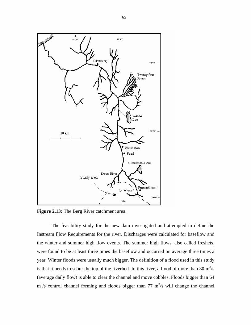
65
Figure 2.13: The Berg River catchment area.
The feasibility study for the new dam investigated and attempted to define the
Instream Flow Requirements for the river. Discharges were calculated for baseflow and
the winter and summer high flow events. The summer high flows, also called freshets,
were found to be at least three times the baseflow and occurred on average three times a
year. Winter floods were usually much bigger. The definition of a flood used in this study
is that it needs to scour the top of the riverbed. In this river, a flood of more than 30 m3/s
(average daily flow) is able to clear the channel and move cobbles. Floods bigger than 64
m3/s control channel forming and floods bigger than 77 m3/s will change the channel
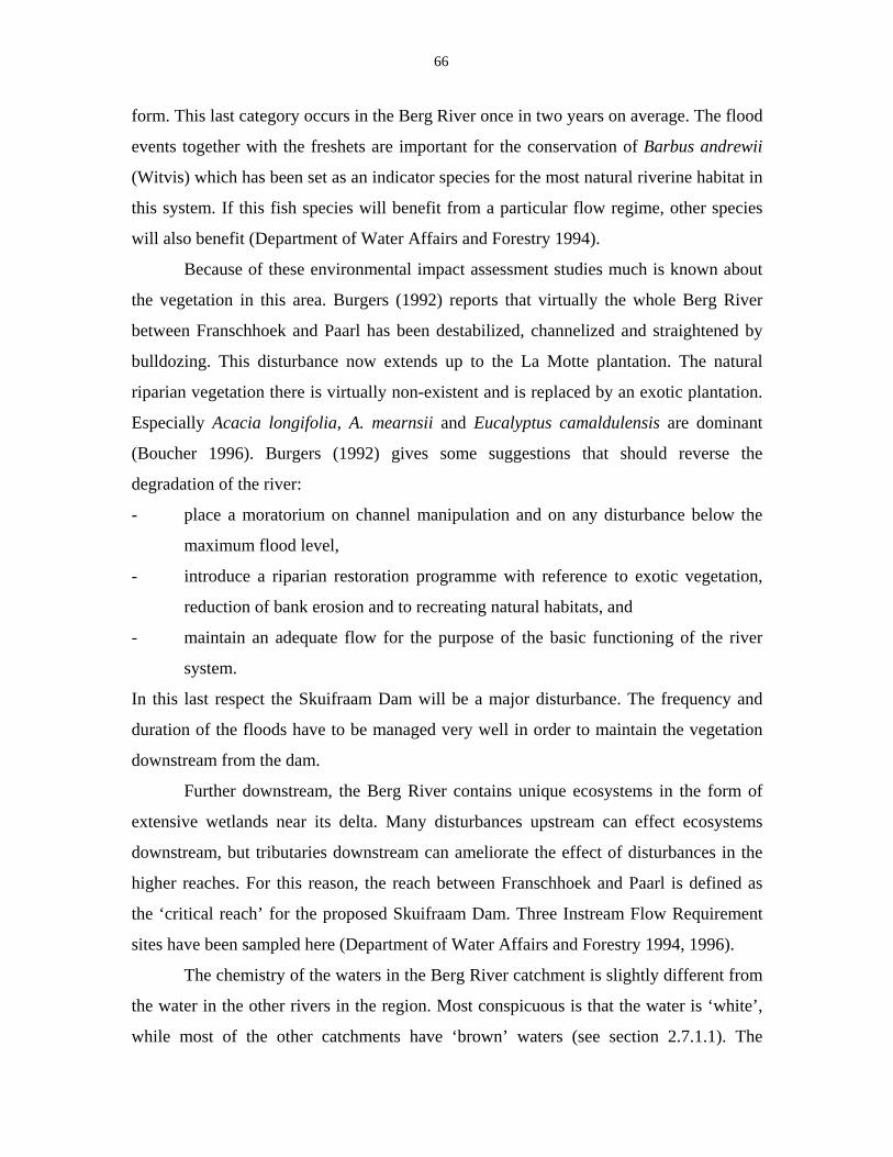
66
form. This last category occurs in the Berg River once in two years on average. The flood
events together with the freshets are important for the conservation of Barbus andrewii
(Witvis) which has been set as an indicator species for the most natural riverine habitat in
this system. If this fish species will benefit from a particular flow regime, other species
will also benefit (Department of Water Affairs and Forestry 1994).
Because of these environmental impact assessment studies much is known about
the vegetation in this area. Burgers (1992) reports that virtually the whole Berg River
between Franschhoek and Paarl has been destabilized, channelized and straightened by
bulldozing. This disturbance now extends up to the La Motte plantation. The natural
riparian vegetation there is virtually non-existent and is replaced by an exotic plantation.
Especially Acacia longifolia, A. mearnsii and Eucalyptus camaldulensis are dominant
(Boucher 1996). Burgers (1992) gives some suggestions that should reverse the
degradation of the river:
- place a moratorium on channel manipulation and on any disturbance below the
maximum flood level,
- introduce a riparian restoration programme with reference to exotic vegetation,
reduction of bank erosion and to recreating natural habitats, and
- maintain an adequate flow for the purpose of the basic functioning of the river
system.
In this last respect the Skuifraam Dam will be a major disturbance. The frequency and
duration of the floods have to be managed very well in order to maintain the vegetation
downstream from the dam.
Further downstream, the Berg River contains unique ecosystems in the form of
extensive wetlands near its delta. Many disturbances upstream can effect ecosystems
downstream, but tributaries downstream can ameliorate the effect of disturbances in the
higher reaches. For this reason, the reach between Franschhoek and Paarl is defined as
the ‘critical reach’ for the proposed Skuifraam Dam. Three Instream Flow Requirement
sites have been sampled here (Department of Water Affairs and Forestry 1994, 1996).
The chemistry of the waters in the Berg River catchment is slightly different from
the water in the other rivers in the region. Most conspicuous is that the water is ‘white’,
while most of the other catchments have ‘brown’ waters (see section 2.7.1.1). The
67
general rule is that the darker the waters are, the more acidic it is. In this case, the Berg
River is an exception, because the water is also acidic (pH 4.3-5.6) (King & Day 1979).
2.7.4.3 Riviersonderend River
The whole northeastern part of the study area is drained by the Riviersonderend River.
The main tributaries of this catchment are the Riviersonderend Kloof, Boegoekloof,
Noordekloof, Boesmanskloof and Dutoits Rivers (see Figure 2.1). The Riviersonderend
River rises at an altitude of approximately 1590 m in Somerset Sneeukop. All the above-
mentioned tributaries flow into the Theewaterskloof Dam, which is situated at an altitude
of 300 m. Further downstream the Riviersonderend River is joined by tributaries draining
the Riviersonderend Mountains. After about 100 kilometres it flows into the Breede
River near Swellendam (Figure 2.14; Ractliffe et al. 1996).
The Theewaterskloof Dam was built in 1979 but only reached full capacity in
1993. The impoundment acts as the source reservoir for the Riviersonderend-Berg-Eerste
River Government Water Scheme. It supplies water to Greater Cape Town, Stellenbosch,
Franschhoek and Paarl and to four agricultural areas: the Riviersonderend River Valley,
the Eerste River Valley, the Berg River Valley and the Overberg Area (Petitjean 1987).
When the dam will receive water from the Skuifraam Dam in the Berg River, the water
level might be raised by a maximum of 0.7 m. Since the dam reached its full capacity in
1993, the river downstream from the dam showed a marked departure from its original
state, particularly in respect of the flood periods and flood peaks. Delays of up to three
months from the first winter floods have been recorded. Now these usually occur in July
and August, while they used to be in April and May in the pre-dam period. The period
with winter floods is also much shorter now. The decrease in the baseflow is most severe
in the periods that are transitional between wet and dry, sometimes endangering the basic
living conditions for the aquatic biota. On the other hand, however, releases of water in
summer for irrigation have doubled the summer baseflows. The impact of the dam is the
greatest immediately downstream from the dam; the runoff from the Riviersonderend
Mountains ameliorates the effects of the dam to a certain extent. The absence of large
scouring floods downstream of the dam resulted in the encroachment of bankside
68
vegetation, especially aliens, into the riverbed and in the deposition of fine particles in
shallow riffle and run areas (Ractliffe et al. 1996).
Figure 2.14: The Riviersonderend catchment area. Note that the upper reaches of the Breede River are not on this map. The geology in the different reaches of the river has its influence on the water
quality (see Figure 2.6). The headwaters of the Riviersonderend River are strongly acidic
because of the highly leached soils in this area. Acidity fluctuates seasonally with
generally lower pH values in winter. The headwaters also have very low concentrations
of major ions but these increase downstream of Theewaterskloof Dam. Partially this can
be explained by the different geological formations in the lower reaches of the river
(Bokkeveld Group shales), but they are also a consequence of agricultural activities
(Ractliffe et al. 1996).
A conservation status assessment has been conducted for the whole river
(Ractliffe et al. 1996). The conservation status gives an indication of how much an
ecosystem has changed from its natural state due to anthropogenic factors. These factors
can be abiotic, such as water abstractions, weirs, dams and pollution, or biotic such as
infestation with alien plants or animals. The riparian zonation patterns have also been
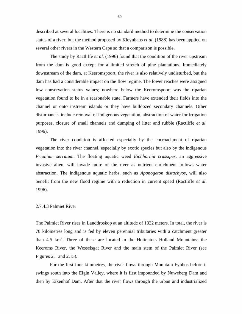
69
described at several localities. There is no standard method to determine the conservation
status of a river, but the method proposed by Kleynhans et al. (1988) has been applied on
several other rivers in the Western Cape so that a comparison is possible.
The study by Ractliffe et al. (1996) found that the condition of the river upstream
from the dam is good except for a limited stretch of pine plantations. Immediately
downstream of the dam, at Keeromspoort, the river is also relatively undisturbed, but the
dam has had a considerable impact on the flow regime. The lower reaches were assigned
low conservation status values; nowhere below the Keeromspoort was the riparian
vegetation found to be in a reasonable state. Farmers have extended their fields into the
channel or onto instream islands or they have bulldozed secondary channels. Other
disturbances include removal of indigenous vegetation, abstraction of water for irrigation
purposes, closure of small channels and dumping of litter and rubble (Ractliffe et al.
1996).
The river condition is affected especially by the encroachment of riparian
vegetation into the river channel, especially by exotic species but also by the indigenous
Prionium serratum. The floating aquatic weed Eichhornia crassipes, an aggressive
invasive alien, will invade more of the river as nutrient enrichment follows water
abstraction. The indigenous aquatic herbs, such as Aponogeton distachyos, will also
benefit from the new flood regime with a reduction in current speed (Ractliffe et al.
1996).
2.7.4.3 Palmiet River
The Palmiet River rises in Landdroskop at an altitude of 1322 meters. In total, the river is
70 kilometres long and is fed by eleven perennial tributaries with a catchment greater
than 4.5 km2. Three of these are located in the Hottentots Holland Mountains: the
Keeroms River, the Wesselsgat River and the main stem of the Palmiet River (see
Figures 2.1 and 2.15).
For the first four kilometres, the river flows through Mountain Fynbos before it
swings south into the Elgin Valley, where it is first impounded by Nuweberg Dam and
then by Eikenhof Dam. After that the river flows through the urban and industrialized
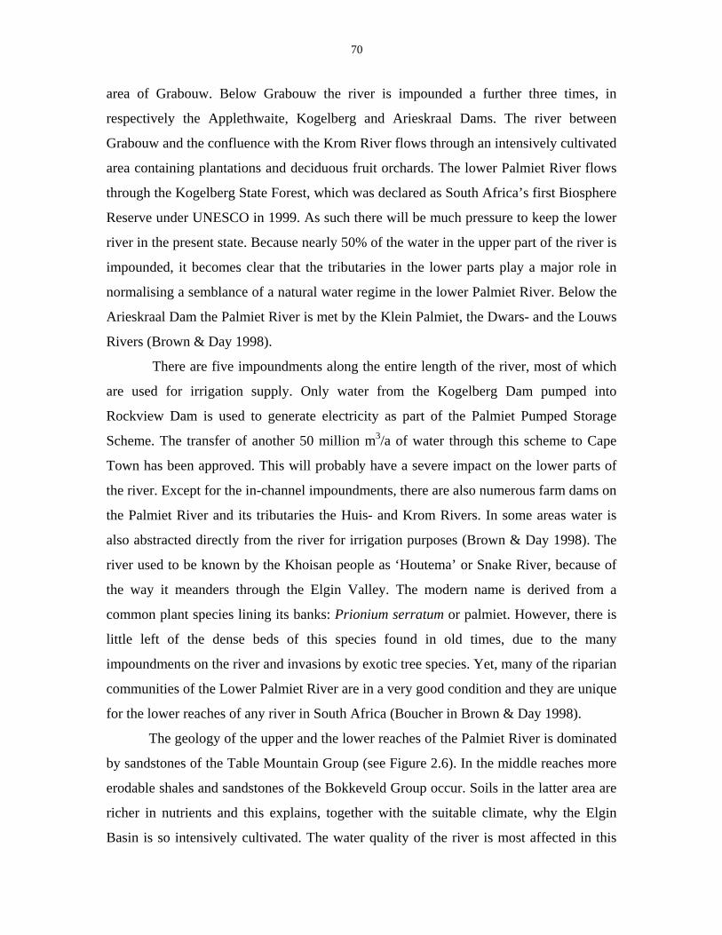
70
area of Grabouw. Below Grabouw the river is impounded a further three times, in
respectively the Applethwaite, Kogelberg and Arieskraal Dams. The river between
Grabouw and the confluence with the Krom River flows through an intensively cultivated
area containing plantations and deciduous fruit orchards. The lower Palmiet River flows
through the Kogelberg State Forest, which was declared as South Africa’s first Biosphere
Reserve under UNESCO in 1999. As such there will be much pressure to keep the lower
river in the present state. Because nearly 50% of the water in the upper part of the river is
impounded, it becomes clear that the tributaries in the lower parts play a major role in
normalising a semblance of a natural water regime in the lower Palmiet River. Below the
Arieskraal Dam the Palmiet River is met by the Klein Palmiet, the Dwars- and the Louws
Rivers (Brown & Day 1998).
There are five impoundments along the entire length of the river, most of which
are used for irrigation supply. Only water from the Kogelberg Dam pumped into
Rockview Dam is used to generate electricity as part of the Palmiet Pumped Storage
Scheme. The transfer of another 50 million m3/a of water through this scheme to Cape
Town has been approved. This will probably have a severe impact on the lower parts of
the river. Except for the in-channel impoundments, there are also numerous farm dams on
the Palmiet River and its tributaries the Huis- and Krom Rivers. In some areas water is
also abstracted directly from the river for irrigation purposes (Brown & Day 1998). The
river used to be known by the Khoisan people as ‘Houtema’ or Snake River, because of
the way it meanders through the Elgin Valley. The modern name is derived from a
common plant species lining its banks: Prionium serratum or palmiet. However, there is
little left of the dense beds of this species found in old times, due to the many
impoundments on the river and invasions by exotic tree species. Yet, many of the riparian
communities of the Lower Palmiet River are in a very good condition and they are unique
for the lower reaches of any river in South Africa (Boucher in Brown & Day 1998).
The geology of the upper and the lower reaches of the Palmiet River is dominated
by sandstones of the Table Mountain Group (see Figure 2.6). In the middle reaches more
erodable shales and sandstones of the Bokkeveld Group occur. Soils in the latter area are
richer in nutrients and this explains, together with the suitable climate, why the Elgin
Basin is so intensively cultivated. The water quality of the river is most affected in this
71
area. Runoff from the agricultural lands causes elevated loads of nutrients and silt. Loads
of silt result in higher turbidity levels and this again results in less light penetration, low
primary production and less food available for organisms higher in the food chain. The
accumulation of nutrients causes eutrophication and the increased presence of algae,
which may become pests. Fertilisers and biocides are frequently applied on agricultural
land and this occasionally leads to runoff of toxins into the river (Brown & Day 1998).
Afforestation, which is quite extensive a little upstream from the agricultural area, can
cause a lot of erosion and thus a higher silt load, especially during periods when the soil
is left exposed before trees are planted (Brown & Day 1998).
In an ecological status assessment conducted in 1998 the worst impacted part of
the river appeared to be the area between the N2 and the confluence of the Klein Palmiet
River, which is seriously modified, while the upper and the lower reaches are largely
natural with few modifications (Brown & Day 1998). The desired state of the river was
determined in a sociological study undertaken by Dr. B. Gale in 1998 in which as many
interested and affected parties were asked about their needs and wants. The river in the
immediate vicinity of Grabouw is mostly used for agricultural, domestic and industrial
purposes, while the lower reaches and the estuary are given a high rating for recreation
and conservation. People living in the catchment area indicate a strong desire for this part
of the river to be maintained or improved (Brown & Day 1998).
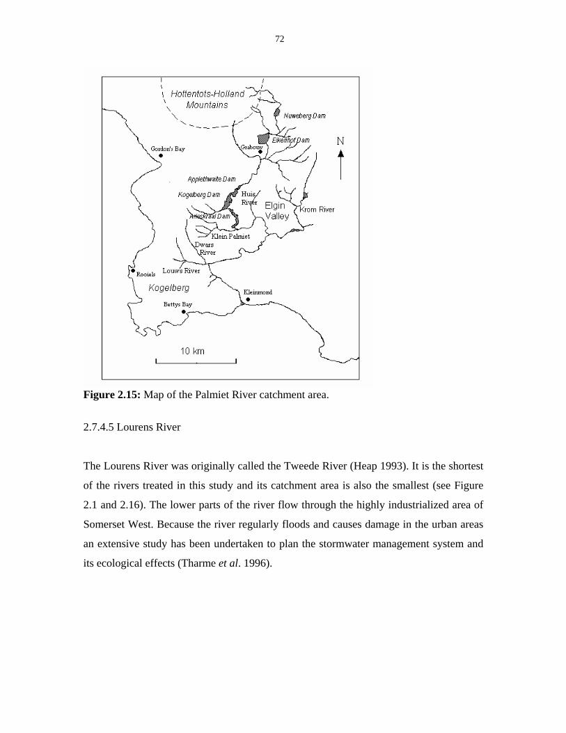
72
Figure 2.15: Map of the Palmiet River catchment area.
2.7.4.5 Lourens River
The Lourens River was originally called the Tweede River (Heap 1993). It is the shortest
of the rivers treated in this study and its catchment area is also the smallest (see Figure
2.1 and 2.16). The lower parts of the river flow through the highly industrialized area of
Somerset West. Because the river regularly floods and causes damage in the urban areas
an extensive study has been undertaken to plan the stormwater management system and
its ecological effects (Tharme et al. 1996).
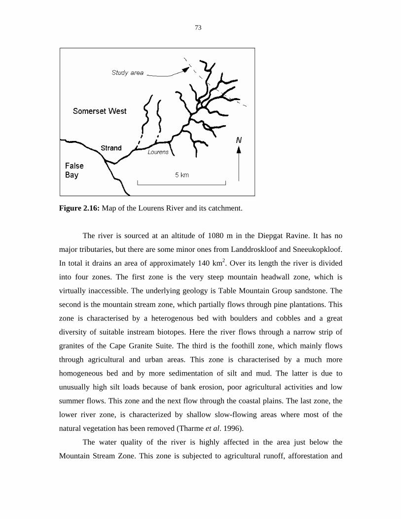
73
Figure 2.16: Map of the Lourens River and its catchment.
The river is sourced at an altitude of 1080 m in the Diepgat Ravine. It has no
major tributaries, but there are some minor ones from Landdroskloof and Sneeukopkloof.
In total it drains an area of approximately 140 km2. Over its length the river is divided
into four zones. The first zone is the very steep mountain headwall zone, which is
virtually inaccessible. The underlying geology is Table Mountain Group sandstone. The
second is the mountain stream zone, which partially flows through pine plantations. This
zone is characterised by a heterogenous bed with boulders and cobbles and a great
diversity of suitable instream biotopes. Here the river flows through a narrow strip of
granites of the Cape Granite Suite. The third is the foothill zone, which mainly flows
through agricultural and urban areas. This zone is characterised by a much more
homogeneous bed and by more sedimentation of silt and mud. The latter is due to
unusually high silt loads because of bank erosion, poor agricultural activities and low
summer flows. This zone and the next flow through the coastal plains. The last zone, the
lower river zone, is characterized by shallow slow-flowing areas where most of the
natural vegetation has been removed (Tharme et al. 1996).
The water quality of the river is highly affected in the area just below the
Mountain Stream Zone. This zone is subjected to agricultural runoff, afforestation and
74
severe erosion. It has a high impact on the zones downstream of it, although the impact
decreases with distance further downstream.
Within the borders of the Hottentots Holland Nature Reserve, the vegetation
around the river is still pristine but the number of exotics increases downstream. A
special threat is kikuyu grass (Pennisetum clandestinum) which forms monospecific
stands that suppress the growth of shrubs and herbs usually found next to rivers. There
are also the usual exotic trees such as Acacia longifolia, A. saligna and Sesbania punicea
(Boucher, in Tharme et al. 1996).
A river conservation status assessment has been made for the Lourens River. The
conservation status decreases downstream. The most serious problems are:
- removal of indigenous vegetation and infestations of exotics,
- decrease of water quality because of various effluents,
- overabstraction of water,
- dumping of rubbish and litter,
- physical manipulation of the river channel to prevent flooding and erosion, and
- settlement of solids because of erosion.
Due to the efforts of the Lourens River Conservation Society, the river gained the Status
of Protected Natural Area in 1997, which offers one of the highest forms of legal
protection for a natural ecosystem (Tharme et al. 1996).
Because the Lourens River flows through a highly urbanized area it also faces a
special problem. The hardening of the surrounding catchment area through the
construction of houses, roads and other infrastructure has increased the runoff to the river
beyond its natural capacity. This causes more and more serious flooding. One-in-twenty
year floodlines become one-in-five year floodlines and areas that are seldom flooded in
natural conditions are flooded regularly. A diversion canal for high floods would be
ecologically the most responsible way to deal with this problem (Tharme et al. 1996).
75
3. Methods used in this study
3.1 The Braun-Blanquet method
The method of describing and investigating vegetation that is used in this study is the
Braun-Blanquet method (Westhoff & Van der Maarel 1973; Werger 1974). This method
is the most widely used method of describing and classifying vegetation at the end of the
twentieth century and has borrowed concepts from many different and divergent
traditions in that century (Whittaker 1962). Most prominent among these are the
‘individualistic concept’ (Gleason 1917, 1926, 1939), which stresses the continuum in
vegetation patterns, and the ‘holistic’ concept (Clements 1916, 1928), which stresses the
existence of plant communities. For a detailed description of the Braun-Blanquet method
and its development see the following references: Braun-Blanquet (1928); Tansley
(1939); Whittaker (1962, 1973a); Shimwell (1971); Mueller-Dombois & Ellenberg
(1974); Westhoff & Van der Maarel (1973); Kent & Coker (1992); Westhoff & De Smidt
(1995) and Mucina (1997).
The most important addition to the ‘classical’ approach of classification is the use
of multivariate techniques to expose gradients within the vegetation (Bray & Curtis 1957;
Whittaker 1967). These authors regard vegetation as a continuum across the landscape
that is determined by environmental gradients. Especially after the introduction of
information technology to ecology different types of ordination techniques were
developed to expose these environmental gradients (Hill 1973, 1974; Hill & Gauch 1980;
Ter Braak 1986, 1987). Some of these techniques make use of linear response curves of
plant species to environmental gradients, while others make use of the Weighted
Averaging method (Curtis & McIntosh 1951) to apply it to unimodal response curves.
The techniques used in this study are mainly Correspondence Analysis or CA (Hill 1974)
and Canonical Correspondence Analysis or CCA (Ter Braak 1986, 1987). A detailed
description of the different ordination techniques can be found in Gauch (1982), Pielou
(1984), Jongman et al. (1987), Ter Braak & Prentice (1988) and Legendre & Legendre
(1999).
76
Nowadays, gradient analysis and classification are no longer seen as contradictory
approaches to the study of vegetation. In most modern studies, vegetation research or
phytosociology uses a combination of both approaches (Whittaker 1972; Westhoff & Van
der Maarel 1973; Van der Maarel 1975). Even classification has been aided by
multivariate statistics (Goodall 1973). The development of TWINSPAN (Hill 1979)
provided an objective manner to classify vegetation types, although manual tabulation
still plays an important role as well (Feoli & Orloci 1983).
3.2 A uniform approach ?
Since the Braun-Blanquet approach was introduced to the Fynbos Biome by Werger et al.
(1972), much discussion has been going on about whether this approach is applicable in
the fynbos or in species-rich environments in general.
One of the opponents to the application of the Braun-Blanquet method in the
Fynbos Biome is B.M. Campbell. This author argues the identification of hundreds of
different species will make classification nearly impossible. On more theoretical grounds
his arguments concern the high gamma diversity in the Fynbos Biome. The turnover of
species between the different mountain ranges is so high that environmentally and
structurally similar communities will have a completely different species composition on
different localities. In a flora with a turnover like this a structural-functional classification
is more likely to be effective in revealing ecological gradients than a floristic
classification (Campbell 1985, 1986a). It is true that in other species-rich areas in the
world, the structural approach is often preferred because of taxonomic and practical
problems. Shimwell (1971) refers to this as ‘the tropical tradition’. Although Werger &
Sprangers (1982) conclude that their floristic and structural classifications of tropical dry
forests in India do not differ too much from each other, they also prefer a floristic
analysis because it reveals more about the ecological position of the vegetation within the
complex of all communities. The decision on whether to choose a floristic or a structural
classification is also largely dependent on the aims of the study.
Other counter-arguments are offered by Boucher (1987) and McDonald &
Boucher (1999). It is true that there are still a lot of taxonomic problems in the Fynbos
77
Biome, but these generally concern the rare species while phytosociology is more
concerned with general species. Turnover between species also often concerns related
species and is especially high on the intraspecific level. Phytosociology does not only use
one specific taxonomic level. In some cases, if it is ecologically or biogeographically
significant, even an entire genus can be used as a characteristic taxon (Westhoff & Van
der Maarel 1973). Turnover itself can only be examined precisely by comparing similar
biotopes across the biome. The high gamma diversity also reflects the climatic gradients
which are very strong in the Cape. The problem with the identification of species also
affects the accuracy of the study. Only proper herbarium specimens are suitable for
secure identification by a taxonomist, but most of the specimens encountered during
vegetation surveys are in a vegetative state. Therefore, the researcher can best build his
collections into a field herbarium of reference specimens, to assist him with the quick
identification of vegetative or otherwise imperfect specimens.
Campbell (1985, 1986a, 1986b) developed a classification of the entire mountain
vegetation of the Fynbos Biome on structural grounds. This classification is very suitable
when a preliminary vegetation survey in a specific area is needed. A phytosociological
study, however, is able to explain more detail about the specific area in question and the
data can be used for further analysis afterwards (see also Boucher 1987).
The first phytosociological studies in the Fynbos Biome were carried out in the
sixties and seventies (see Table 2.3 for references). During the eighties many other
studies followed, but the east and the northwest of the biome are still under-represented.
Data from the many studies are integrated in the VEGMAP project (McDonald 1997;
Mucina et al. 2000) in which the classification of the entire Fynbos Biome has been
achieved to the level of the vegetation class.
The most notable difficulty with the Braun-Blanquet method in the Fynbos Biome
is the characterization of communities by character species, because a character species,
sensu stricto, is a species that occurs in one community type only and differentiates it
from all other community types. Because of the strong ecological gradients occurring in
the Fynbos Biome, a species that is a character species for a specific community in one
area can be a character species for another in another area, in other words these species
are only local character species (Shimwell 1971). Regional character species are only
78
represented by the endemics and these cannot be used when vegetation units of different
mountain areas are compared with each other. One can argue that the use of character
species was over-emphasized in the European context. In any event, the first priority is to
develop a skeleton of syntaxonomic systems for the region, before researchers can
realistically discern between character and differential species.
The information value of vegetation classification is increased considerably if the
classification is combined with gradient analysis, especially in this biome where
gradients abound. After the ecological significance of a species has been revealed
through ordination techniques, their role in the classification and the characterization of
communities is far more obvious. Autecological studies on dominant or differential
species will also increase the understanding of this complex vegetation.
3.3 The sampling method
According to the Braun-Blanquet approach, vegetation samples need to be taken from
homogeneous stands of vegetation. Several theories have been developed about how to
deal with issues like homogeneity, sample size, sample number, stratification and
measurement of abundance. Most of these are summarized by Mueller-Dombois &
Ellenberg (1974), Werger (1974), Westhoff & Van der Maarel (1973) and Whittaker
(1973a).
3.3.1 Homogeneity
A vegetation sample suitable for analysis using the Braun-Blanquet approach, also called
a relevé, has to be homogeneous or uniform. This is the main criterion for the choice of
the plots by the researcher. A homogeneous plot contains one vegetation type. There
should be no obvious structural boundary in the plot. Differences in floristic composition
within the plot are not allowed. It is common practice for a researcher to look for
differences in dominant and abundant species in the research area and on this basis to
define the different vegetation stands beforehand. Within these stands the contents of a
79
number of homeogeneous sample plots can be recorded (Westhoff & Van der Maarel
1973).
The condition of homogeneity has a very important influence on the choice of
sample plots. It has often been commented that the choice of the sample plots is
subjective and thus less valid. The American researchers, in contrast, have often favoured
a system of randomized plots. However, nearly every empirical science has to deal with
the subjective choices of the researcher. Randomization of sample plots seems to have
little effect on the results except that many samples have to be discarded because of
heterogeneity, which results in a waste of research time (Whittaker 1973a).
3.3.2 Sample size
The size of a sample is largely dependent on the vegetation structure but if the vegetation
stand is sufficiently small, it may be sampled entirely in one plot. The size of a sample
quadrat in larger stands should be large enough to contain all the species of regular
occurrence in that stand. The ideal size for a plot can be determined by successively
doubling the surface area of a sample quadrat and counting the number of species in all
respective plots. The resulting species-area curve levels off at a certain stage and this area
can be taken as the minimal area (Barkman 1989; Kenkel & Podani 1991; Kent & Coker
1992).
Westfall et al. (1987) have determined a formula to predict the number of species
in a given area in the Waterberg in the Northwest Province of South Africa. With this
formula they can calculate the rate at which species numbers increase with increasing
surface area. When the increment of species is less than 10%, the optimal sample size is
reached.
Van der Maarel (1996) argues that strict application of the minimal area concept
may underestimate species capture, due to small-scale dynamics and proposed instead to
use a maximum area. Wilson & Chiarucci (2000) have extrapolated the species per unit
area to the landscape and regional levels. They made the rigorous conclusion that
‘homogeneous communities’ do not exist and that everything depends on the hierarchical
scale at which the study is levelled.
80
Through the experience of many experts, the optimal sample area for different
(physiognomic) vegetation types worldwide has been determined. For equivalent
vegetation types that occur within the Fynbos Biome the values are as follows:
Hygrophilous (Wet Bank) communities: 1–4 m2, temperate sclerophyllous shrublands
(fynbos): 10–100 m2, scrub: 25–100 m2 and temperate deciduous forests: 100–500 m2
(Westhoff & Van der Maarel 1973, see also Tüxen 1970).
In the case of transects used to sample lateral river gradients, the size of the stand
is often limited by topographic features, but the minimal sizes for the different
community types fit well within the surface areas obtained in a transect placed across a
river with a transect width of 10 metres.
3.3.3 Number of samples
For a good description of the vegetation according to the Braun-Blanquet method it is
necessary that there are sufficient samples in every vegetation type under study and no
type is under- or over-represented. At the same time, the researcher aims to obtain
vegetation samples that from the entire study area to make sure that as many variations as
possible are covered. Thus, before or during the sampling process, the researcher already
makes some preliminary classifications so that the number of samples of undersampled
communities can be supplemented. Unstable or mixed samples have to be removed
afterwards (Westhoff & Van der Maarel 1973).
In this study, the number of units that could be sampled was limited by a
devastating fire that raged through the study area during April 1999, before all the field
work was finished. After this some rare vegetation types could still be sampled in
unburnt islands or marginal areas. But the data set still contains some vegetation types
that are undersampled, as the fynbos in the Hottentots Holland Mountains will only be in
a mature condition, sufficient to identify persistent species, in 5-6 years after being burnt
(Van der Merwe 1966). Some additional samples were obtained from neighbouring areas
to reduce this shortcoming in the data set.
3.3.4 Stratification
81
The description of vegetation strata forms an important part of the structural
characterization of the vegetation. Early methods of vegetation classification were mainly
based on structural data (Shimwell 1971; Mueller-Dombois & Ellenberg 1974). It is often
possible to link different floristic vegetation units together into several ‘structural groups’
afterwards. Campbell (1986a) undertook a structural classification of montane vegetation
in the Fynbos Biome, and he argues that a detailed, floristic classification in the biome is
not feasible, because species turnover between mountain ranges is too high, although he
made considerable use of floristic features in his structural classification.
Four different strata are broadly recognized in the present study of riparian
vegetation, namely, the tree, shrub, herb and moss layers. Mosses have only been
recorded in the Wet Bank Zone (Figure 2.10). The shrub layer has been divided into a
higher (2–6 m) and a lower shrub layer (0.5–2 m). Elsewhere in the Fynbos Biome,
different layers can be recognised within the tree layer, but none of the tree species
occurring in the Hottentots Holland area exceeds 12 metres, so they are all recognised as
belonging to the same layer (6–12 m). These vegetation layers are defined in the
vegetation database program Turboveg (Hennekens 1996).
3.3.5 Coverage and abundance
In every sample taken in the present study the species are recorded together with the
vegetation stratum to which they belong and their projected canopy cover in the Braun-
Blanquet or the ordinal scale is estimated. The definition of the ordinal scale compared to
the traditional and the extended Braun-Blanquet scale is presented in Table 3.1. There is
no real difference between the scales: the ordinal scale was introduced in order to
simplify the notation. I recorded vegetation samples using the ordinal scales, which I
later converted to the extended Braun-Blanquet scale for analysis and descriptive
purposes.
In this study, a herbarium specimen was collected of each of the species
encountered to serve as a voucher specimen for identification and for reference purposes.
Later records of a species refer to this specimen. The specimens were identified by the
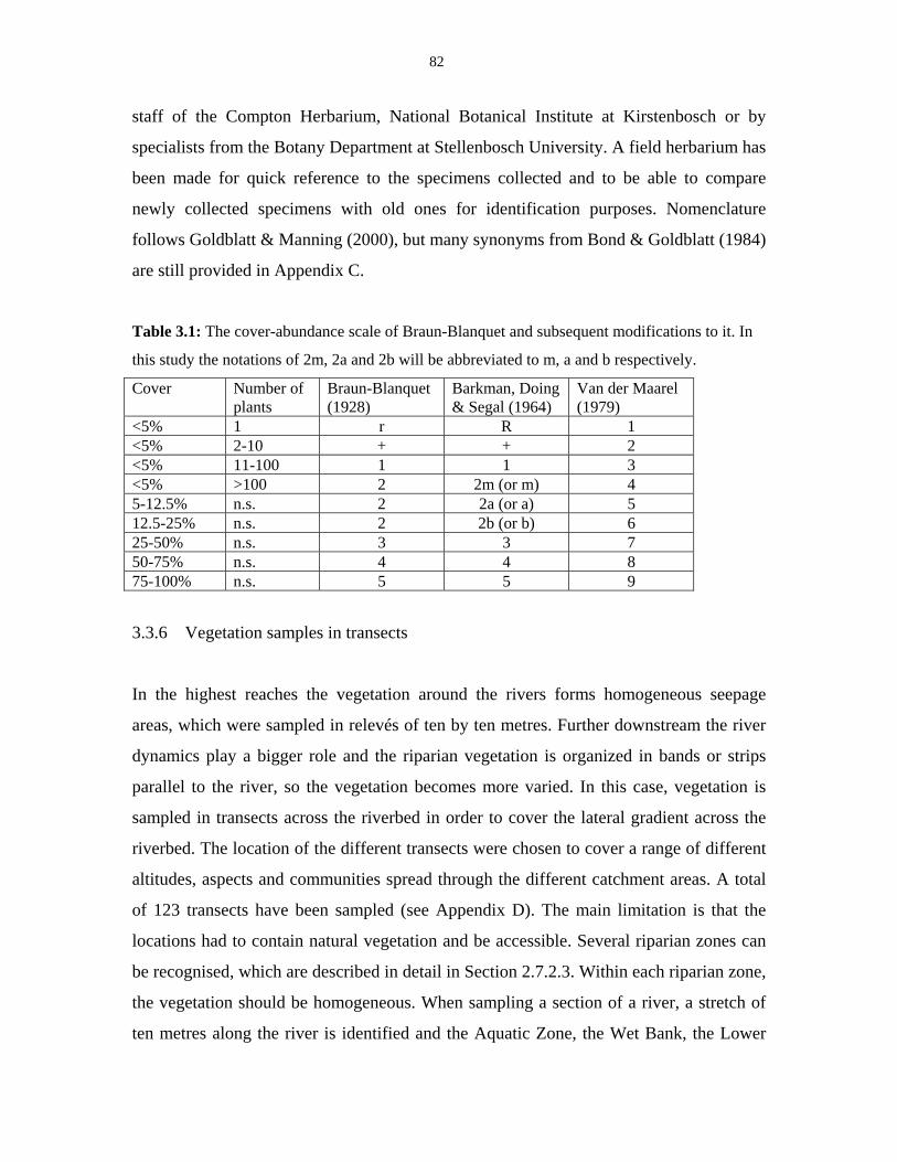
82
staff of the Compton Herbarium, National Botanical Institute at Kirstenbosch or by
specialists from the Botany Department at Stellenbosch University. A field herbarium has
been made for quick reference to the specimens collected and to be able to compare
newly collected specimens with old ones for identification purposes. Nomenclature
follows Goldblatt & Manning (2000), but many synonyms from Bond & Goldblatt (1984)
are still provided in Appendix C.
Table 3.1: The cover-abundance scale of Braun-Blanquet and subsequent modifications to it. In
this study the notations of 2m, 2a and 2b will be abbreviated to m, a and b respectively.
Cover Number of plants
Braun-Blanquet (1928)
Barkman, Doing & Segal (1964)
Van der Maarel (1979)
<5% 1 r R 1 <5% 2-10 + + 2 <5% 11-100 1 1 3 <5% >100 2 2m (or m) 4 5-12.5% n.s. 2 2a (or a) 5 12.5-25% n.s. 2 2b (or b) 6 25-50% n.s. 3 3 7 50-75% n.s. 4 4 8 75-100% n.s. 5 5 9
3.3.6 Vegetation samples in transects
In the highest reaches the vegetation around the rivers forms homogeneous seepage
areas, which were sampled in relevés of ten by ten metres. Further downstream the river
dynamics play a bigger role and the riparian vegetation is organized in bands or strips
parallel to the river, so the vegetation becomes more varied. In this case, vegetation is
sampled in transects across the riverbed in order to cover the lateral gradient across the
riverbed. The location of the different transects were chosen to cover a range of different
altitudes, aspects and communities spread through the different catchment areas. A total
of 123 transects have been sampled (see Appendix D). The main limitation is that the
locations had to contain natural vegetation and be accessible. Several riparian zones can
be recognised, which are described in detail in Section 2.7.2.3. Within each riparian zone,
the vegetation should be homogeneous. When sampling a section of a river, a stretch of
ten metres along the river is identified and the Aquatic Zone, the Wet Bank, the Lower
83
Dynamic, the Shrub/Tree and the Back Dynamic Zones are each sampled separately.
Glavaç et al. (1992) mention an example of riverine floodplains where the vegetation
borders are very sharp even though the elevation gradient extends across the whole
floodplain. With this example they demonstrate that riverine vegetation perfectly suits the
discontinuum theory. The situation in mountain streams is quite different because banks
are quite steep, but the vegetation borders are equally sharp.
When sampling takes place along a transect, there are a few considerations to be
made. The first one concerns the size of the different samples within the transect. The
surface area covered by a particular vegetation unit is dependent on the width of the
riparian zone in which it occurs. When a riverbank is steep, zones are narrow and will
have a smaller surface area and when banks are flat, the respective zones are wide and
the surface areas within the sample are large. In general, however, the same type of
vegetation zone will be represented in more or less equally sized samples. Wet Bank
Zones are often very narrow, because they only occur in the area where small
fluctuations in the water level inundate the substrate. They are often also fragmented and
can be broken up by large rocks and boulders. In a stretch of ten metres, a Wet Bank
Zone can be quite heterogeneous while the other riparian zones further up the bank are
homogeneous. Back Dynamic Zones and Shrub/Tree Zones are represented in wider
zones and can be sampled in an area that is large enough for that type of vegetation (see
section 3.3.2). The sampling of relevés with different surface areas from the same river
zone but in different transects is a problem that is difficult to avoid given the variability
in the physiography of the terrain. It is assumed that this does not have a major effect as
long as the differences in sample size are not extreme. An attempt was made to stick to
comparable sample sizes for each zone.
Another problem that occurs in transects are heterogeneous samples and the
definition of the borders. Mostly, the vegetation borders on a riverbank are quite sharp,
but where this is not the case an extra sample has to be taken from the ‘transition zone’.
In these instances there might be different samples representing the same riparian zone.
In any event the analysis of the vegetation data is undertaken to include all samples
irrespective of their location.
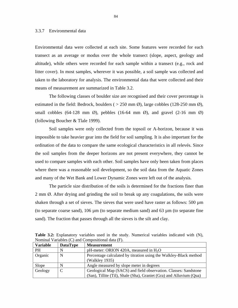
84
3.3.7 Environmental data
Environmental data were collected at each site. Some features were recorded for each
transect as an average or modus over the whole transect (slope, aspect, geology and
altitude), while others were recorded for each sample within a transect (e.g., rock and
litter cover). In most samples, wherever it was possible, a soil sample was collected and
taken to the laboratory for analysis. The environmental data that were collected and their
means of measurement are summarized in Table 3.2.
The following classes of boulder size are recognised and their cover percentage is
estimated in the field: Bedrock, boulders ( > 250 mm Ø), large cobbles (128-250 mm Ø),
small cobbles (64-128 mm Ø), pebbles (16-64 mm Ø), and gravel (2-16 mm Ø)
(following Boucher & Tlale 1999).
Soil samples were only collected from the topsoil or A-horizon, because it was
impossible to take heavier gear into the field for soil sampling. It is also important for the
ordination of the data to compare the same ecological characteristics in all relevés. Since
the soil samples from the deeper horizons are not present everywhere, they cannot be
used to compare samples with each other. Soil samples have only been taken from places
where there was a reasonable soil development, so the soil data from the Aquatic Zones
and many of the Wet Bank and Lower Dynamic Zones were left out of the analysis.
The particle size distribution of the soils is determined for the fractions finer than
2 mm Ø. After drying and grinding the soil to break up any coagulations, the soils were
shaken through a set of sieves. The sieves that were used have raster as follows: 500 µm
(to separate coarse sand), 106 µm (to separate medium sand) and 63 µm (to separate fine
sand). The fraction that passes through all the sieves is the silt and clay.
Table 3.2: Explanatory variables used in the study. Numerical variables indicated with (N), Nominal Variables (C) and Compositional data (F). Variable DataType Measurement PH N pH-meter: ORION 420A, measured in H2O Organic N Percentage calculated by titration using the Walkley-Black method
(Walkley 1935) Slope N Angle measured by slope meter in degrees Geology C Geological Map (SACS) and field observation. Classes: Sandstone
(San), Tillite (Til), Shale (Sha), Graniet (Gra) and Alluvium (Qua)
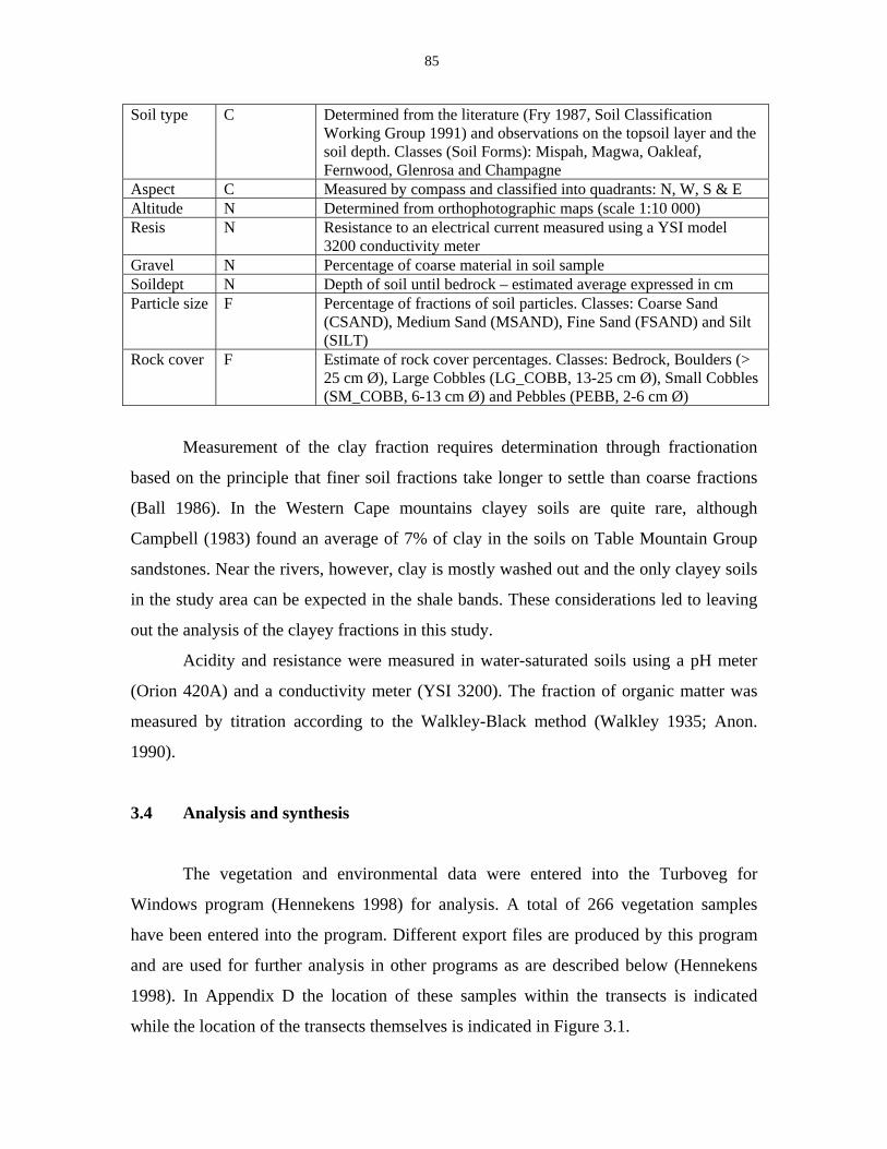
85
Soil type C Determined from the literature (Fry 1987, Soil Classification Working Group 1991) and observations on the topsoil layer and the soil depth. Classes (Soil Forms): Mispah, Magwa, Oakleaf, Fernwood, Glenrosa and Champagne
Aspect C Measured by compass and classified into quadrants: N, W, S & E Altitude N Determined from orthophotographic maps (scale 1:10 000) Resis N Resistance to an electrical current measured using a YSI model
3200 conductivity meter Gravel N Percentage of coarse material in soil sample Soildept N Depth of soil until bedrock – estimated average expressed in cm Particle size F Percentage of fractions of soil particles. Classes: Coarse Sand
(CSAND), Medium Sand (MSAND), Fine Sand (FSAND) and Silt (SILT)
Rock cover F Estimate of rock cover percentages. Classes: Bedrock, Boulders (> 25 cm Ø), Large Cobbles (LG_COBB, 13-25 cm Ø), Small Cobbles (SM_COBB, 6-13 cm Ø) and Pebbles (PEBB, 2-6 cm Ø)
Measurement of the clay fraction requires determination through fractionation
based on the principle that finer soil fractions take longer to settle than coarse fractions
(Ball 1986). In the Western Cape mountains clayey soils are quite rare, although
Campbell (1983) found an average of 7% of clay in the soils on Table Mountain Group
sandstones. Near the rivers, however, clay is mostly washed out and the only clayey soils
in the study area can be expected in the shale bands. These considerations led to leaving
out the analysis of the clayey fractions in this study.
Acidity and resistance were measured in water-saturated soils using a pH meter
(Orion 420A) and a conductivity meter (YSI 3200). The fraction of organic matter was
measured by titration according to the Walkley-Black method (Walkley 1935; Anon.
1990).
3.4 Analysis and synthesis
The vegetation and environmental data were entered into the Turboveg for
Windows program (Hennekens 1998) for analysis. A total of 266 vegetation samples
have been entered into the program. Different export files are produced by this program
and are used for further analysis in other programs as are described below (Hennekens
1998). In Appendix D the location of these samples within the transects is indicated
while the location of the transects themselves is indicated in Figure 3.1.
86
The computer program Megatab (Hennekens 1996) is used for classification. The
TWINSPAN procedure in this program is used to classify the samples in a numerical
way, but this classification is only used as a first draft, after which modifications are
made to the classification order of samples and species based on insight and field
experience, using the options in the Megatab Program.
The ordinations are done using the program Canoco 4.0 (Ter Braak & Šmilauer
1998). Before the ordination of the complete dataset is carried out, the correlations
between the environmental variables are analysed using Principal Components Analysis
(PCA). In this way a choice can be made about the environmental variables suitable for
the ordination of the whole dataset. Correspondence Analysis (CA) is used to investigate
the dataset for trends and gradients within the vegetation itself (indirect gradient analysis;
Hill 1974). After this Canonical Correspondence Analysis (CCA) follows to determine
the relation between the vegetation data and the environmental variables (direct gradient
analysis; Ter Braak 1986). A Monte Carlo permutation test is undertaken to determine
whether the ordination axes have significance (Ter Braak & Šmilauer 1998). The
combination of the use of both CA and CCA is necessary to determine how much of the
variation in the vegetation data is explained by the environmental variables (McDonald et
al. 1996; Brown et al. 1993; Økland 1996).
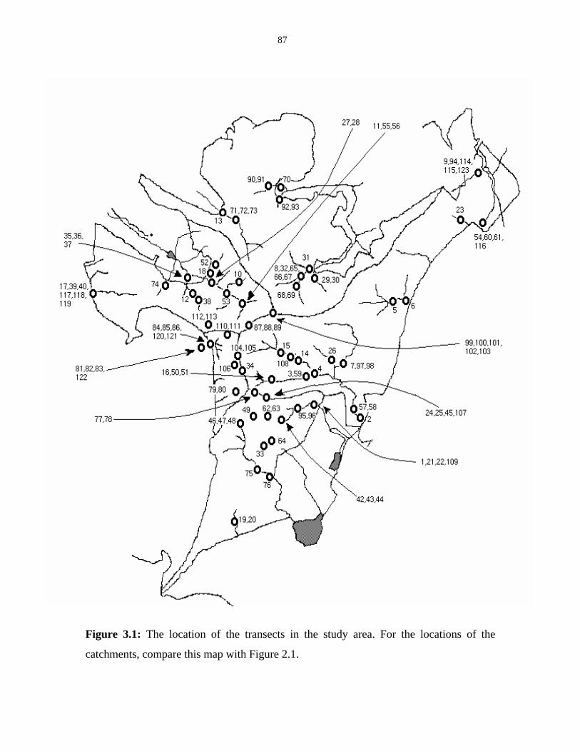
87
Figure 3.1: The location of the transects in the study area. For the locations of the
catchments, compare this map with Figure 2.1.
88
4. High-altitude fen and mire vegetation of the Hottentots Holland
Mountains of the Western Cape, South Africa
4.1 Abstract
A phytosociological survey has been undertaken of the extensive seepage areas occurring
in the Hottentots Holland Mountains, Western Cape, South Africa using the Braun-
Blanquet method. Nine different communities have been recognized, three of which have
been given scientific names following the 3rd edition of the International Code of
Phytosociological Nomenclature.
The most important differentiating feature between the mire communities
described here is the degree of minerotrophy. The soils in the centre of the mires are very
peaty with very little influence from the surrounding sandstone, while the soils on the
margin of the mires have a greater admixture of soil originating from sandstone. Most of
the mire communities described here are dominated by low growing clonal Restionaceae,
such as Anthochortus crinalis, although these can occur in a mosaic with the tall restio
Chondropetalum mucronatum. The mire vegetation in the mountains is vulnerable to
climate change and water abstraction and the results of this study can be used as
reference types for monitoring.
4.2 Introduction
The Western Cape Mountains are important catchments for high-quality drinking
water. A vast quantity of this water is stored after precipitation in the seepage areas
before it enters the river systems. The quality of the water is largely determined by the
soil conditions that the water encounters on its way to the river, so the seepage areas have
a great importance for the river ecosystem (Bosch et al. 1986). However, the Variable
Source Area Concept of Hewlett (1961) states that the catchment area that drains into a
river is variable in size and many seepage areas can be out of touch with the river for a
long time. After heavy rains the Source Area of the river expands and much water that
89
was stored in fens for a long time is washed into the river. This explains the brown colour
of many of the Cape rivers after heavy rains (King & Day 1979).
‘Seepage area’ is a very general term for the source area of a river. It constitutes
all sorts of areas where water moves underground towards the river and includes the
majority of wet slopes but also many mires that occur in mountainous regions. The
definitions of bogs, fens and mires, as they are used in this text, are given by Gore
(1983). Mires are adopted as a general term for wet swampy places, while bogs and fens
are more specific types of mires. The term ‘bog’ refers to the strictly ombrotrophic mires
found in places with high rainfall, while ‘fens’ are the mires that are fed to a certain
extent by water from a minerotrophic origin. Bogs are very rare in the Southern
Hemisphere and are probably absent from the Western Cape.
There are three different types of seepages in the Western Cape Mountains that
form part of the drainage network of the river system:
(1) The seepages on slopes are better drained than the other two types listed
below. They can best be described as Wet Ericaceous Fynbos (Campbell
1986b). The soils here are mostly of the Fernwood Form (Fry 1987). This
seepage type can be characterized by the presence of Bruniaceae, although it
is highly variable.
(2) In the low-altitude seepages in wet valleys the water is stagnant and peaty
Champagne Form soils generally develop here. The vegetation of these
habitats in the Kogelberg Biosphere Reserve was described by Boucher
(1978) as Erica-Osmitopsis Seepage Fynbos. This vegetation type was not
found in the Hottentots Holland Mountains. Another type of low-altitude
seepage occurs on temporarily wet sandy soils and is dominated by Elegia
filacea (Taylor 1978).
(3) The high-altitude fens and mires which are situated at the sources of the rivers
will be described in this paper.
The high-altitude mires form an important part of the river system but they also form an
ecosystem on their own. Rogers (1997) records that the wetland ecosystems in the Cape
mountains have received little attention but deserve a closer look. As most African
90
swamps and mires are dominated by grasses and sedges (Thompson & Hamilton 1983;
Van Zinderen Bakker & Werger 1974), the mires in the Western Cape are conspicuously
different because of the dominance of Restionaceae (Campbell 1986b; Rogers 1997).
This study presents a preliminary description of these ecosystems and gives an insight
into the ecological processes that drive them.
4.3 Study area
The majority of vegetation samples examined in this paper were recorded from
the Hottentots Holland Mountains (between 33º 56’ S and 34º 03’ S latitude and 18º 57’
E and 19º 09’ E longitude, see Figure 2.1). This area, situated between the towns of
Stellenbosch, Franschhoek, Grabouw and Somerset West, has the highest rainfall of the
entire Western Cape. It has many peaks higher than 1000 metres and numerous and
extensive mires have developed here.
Most of the mires are part of the Palmiet River catchment, although the
Riviersonderend River and the Eerste River catchments also receive water from fairly
extensive mire systems. Two other rivers originating in the area, the Berg River and the
Lourens River, barely receive water from mires and have their origin on very steep
mountain headwalls.
4.4 Climate
The climate at high altitude is very different from the climate in the valleys,
because of the gradients in rainfall and temperatures, which vary with changes in altitude
(Versfeld et al. 1992). Sixty per cent of the precipitation falls in the wettest four months,
which is from June to September. This precipitation is mostly in the form of rain but
snow can occur in winter on the mountain peaks (Fuggle & Ashton 1979). An unknown
amount of precipitation occurs in the form of fog, as few stations are designed to record
its occurrence. Although the fog-saturated air definitely has an impact on the physiology
of plants, only very few plants, mainly epiphytes, are able to make direct use of water
from this resource (Kerfoot 1968). Wind speeds are highest in winter on the mountain
91
tops. This is in contrast with the wind in the lowlands, which are highest in summer. In
summer, easterly winds dominate, while the winter brings more westerly winds (Deacon
et al. 1992).
4.5 Geology and soils
The geology of the Hottentots Holland Mountains is dominated by sandstones and
shales of the Table Mountain Group, especially at the higher altitudes. Some of the
valleys are underlain by granite, but no mires were found on this substrate in the present
study. The sandstones are mainly from the Nardouw Formation. A high altitude shale-
band of the Cedarberg Formation accompanied by tillite of the Pakhuis Formation occurs
sporadically through the area (De Villiers et al. 1964). These bands are situated at higher
altitudes than most of the seepage areas and virtually all the vegetation types (with one
exception) described in this study are from sandstone.
Soils of the mires are classified as belonging to the Champagne Form (Soil
Classification Working Group 1991). The amount of peat is variable and, towards the
outer edges of a seepage area, there is a greater proportion of soil originating from
sandstones. Here soils of the Fernwood Form will prevail. In this study, soils have been
used as a major characteristic to delimit the location of the mires sampled in this study.
Vegetation samples have only been taken from the predominantly organic soils of the
Champagne Form. There is, however, still much variation in the proportion of organic
material in the soils.
4.6 Methods
Vegetation sampling followed the Braun-Blanquet Method (Westhoff & Van der Maarel
1973; Werger 1974). The samples taken from the Hottentots Holland Mountains number
33 in total. An additional four samples have been taken from the Dutoitskloof Mountains
to the north of the study area, one from the Groenland Mountains and one from the
Akkedisberg, both located southeast of the study area (see Figure 2.4b). These samples
were taken to get some indication of the degree of turnover in mire vegetation types
92
across the Cape Mountains. Two of these additional samples fitted in well with the
Hottentots Holland data and have been included in the vegetation table (see Appendix E;
Table 1).
The vegetation samples from the Hottentots Holland Mountains have been
classified using a combination of TWINSPAN and manual tabulation (Hill 1979). During
the manual tabulation process, a vegetation scientist assesses the acceptability of the
TWINSPAN components and uses his field knowledge and the particular sites involved
as a reference (Kent & Coker 1992). The aim of manual reshuffling is to cluster samples,
based on the presence and absence of species, as far as possible into blocks (Feoli &
Orloci 1985). The programme used for this purpose is Megatab (Hennekens 1996).
Three well-sampled communities have been given names according to the
international rules for syntaxomic nomenclature of Weber et al. (2000). All communities
have been given a local name based on vegetation structure and two important species,
useful for local reference purposes, following guidelines proposed by Edwards (1983).
All the environmental variables mentioned in Chapter 3 were collected in the
mires. The relationship between the environmental data and the vegetation data was
determined using multivariate techniques. Legendre & Legendre (1998) give a good
overview of the multivariate techniques currently available. Following Økland (1996),
who argues that ordination and constrained ordination complement each other as they
provide different information, both a direct and an indirect gradient analysis were
undertaken in this study. The package of programs that was used for this analysis is
contained in the Canoco 4.0 program suite (Ter Braak & Šmilauer 1998). The
compositional data, such as particle size, were log-transformed prior to further analysis,
according to the recommendations of Ter Braak & Šmilauer (1998). The technique used
for indirect gradient analysis is Correspondence Analysis or CA, which makes use of the
Weighted Averaging algorithm, which makes it applicable for unimodal response curves
(Hill 1974). The technique for direct gradient analysis used in this study is Canonical
Correspondence Analysis or CCA, which constrains the axes found in CA to the
explained variation only by comparing axes based on species data with axes based on
environmental variables (Ter Braak 1986).
93
4.7 Results
Table 1 in Appendix E presents the vegetation table for the mires recorded during this
study. The communities are described here at the level of association. The higher
syntaxonomic levels are not discussed here because they will only become clear after
more data from other mountain ranges becomes available. There are only three
communities that have received an official syntaxomic name following the Code of
Phytosociological Nomenclature (Weber et al. 2000). A type relevé, which is a relevé
that is typical for the vegetation unit and should at least contain all the differential and
name-giving species, is selected for these communities (Weber et al. 2000). The
differential species, constant companions and the dominant species are identified in each
case. A differential species is a species that can be used to differentiate between one
community or a group of communities, and the rest at the same syntaxonomic level
(Westhoff & Van der Maarel 1973). For this, I used a guideline of a difference in
frequency of more than two presence classes (40%). However, a species can also be
called differential on the basis of cover. This guideline is not handled strictly in the case
of communities with few samples. A constant companion is a species that occurs in more
than 60% of all the samples in the community. A dominant species is a species that is
constant and has an average cover of more than 25 % (Westhoff & Van der Maarel
1973).
Generally, mires in the Hottentots Holland Mountains can be recognised by a
high cover of Restionaceae. Only a few seepage types are dominated by grasses or
sedges, such as Pennisetum macrourum, Carpha glomerata, Isolepis prolifer or
Epischoenus spp. More typically, some species of Restionaceae are dominant. The most
common species are Anthochortus crinalis, Chondropetalum mucronatum, Elegia
thyrsifera and Restio subtilis. Two graminoids that are common are Ehrharta setacea ssp.
setacea and Epischoenus villosus. The Asteraceae are represented by Senecio crispus and
Ursinia caledonica. Montane seepages often contain a narrow drainage channel in which
impoverished aquatic or wetbank communities might occur.
Most seepages described here are classified by Campbell (1986b) as Sneeukop
Azonal Restioid Fynbos. They occur in general on deep, dark, organic soils with a pH
94
lower than 4. In order to distinguish between the different degrees of minerotrophy in the
mires described in this study, I want to introduce the term ‘restio marshlands’ for the
communities on the better-drained sites at the edge of a mire in the Western Cape, in
contrast to the ‘fens’ that are situated in the centre of the mire. Community Group 1: Fens
Fens form the wettest parts of the seepages and they are poorly drained. The low growing
restio Anthochortus crinalis is usually dominant and forms dense mats between tussocks
of Epischoenus villosus. The first two communities described here are unusual because
they occur on steep slopes, so they have better drainage despite being very wet.
Community type 1.1: Protea lacticolor-Hippia pilosa Tall Shrubland
Number of relevés: 2
Range of species number: 18 – 20
This community, which is found on the impervious shales of the Cedarberg Formation, is
characterised by a high cover of Protea lacticolor, which is a dominant species. This
proteoid forms a dense shrub layer between about two and four metres tall. This
structural type is not found in any of the other seepage communities and it is the only
form of proteoid fynbos recorded in this study. The herb layer is also very dense and
covers more than 80% of the relevé. Tussocks of Epischoenus villosus and mats of Restio
perplexus (a differential species) define the structure of the herb layer. In between, other
important species can be found, such as Senecio umbellatus, Stoebe plumosa, Hippia
pilosa and Oxalis truncatula. The community occurs on the eastern slopes of Somerset
Sneeukop at a very high altitude on the shaleband. It receives an extremely high annual
rainfall (more than 3 300 mm). It is also likely to receive snow, which persists longer on
the eastern slopes than on the western slopes. Campbell (1986b) refers to this type as
Otterford Wet Proteoid Fynbos.
Community type 1.2: Elegia thyrsifera-Centella eriantha Short Closed Herbland
95
Number of relevés: 2
Range of species number: 15 – 16
This community is found near the sources of the Lourens River on the western slopes of
Somerset Sneeukop. The tall herb layer is formed by the dominance of Elegia thyrsifera
and a short herb layer is occupied by a multitude of other species, such as Senecio
umbellatus, Hippia pilosa and Erica curviflora. This community, like the Protea
lacticolor-Hippia pilosa Tall Shrubland, is quite atypical for seepages in the Hottentots
Holland Mountains. The differential species, Carpacoce spermacocea, Ursinia
eckloniana, Centella eriantha and Othonna quinquedentata, are all more common in
Ericaceous Fynbos communities (See Chapter 5). It occurs on steep slopes on sandstone.
This is the main habitat difference from the former community that occurs on shale. It
occurs, as does the former community, at high altitudes and receives a high precipitation.
Community type 1.3: Anthochortus crinalis-Elegia intermedia Tall Closed Restioland
Scientific name: Anthochorto crinalis-Elegietum intermediae ass. nova hoc loco
Number of relevés: 4
Type relevé: 229 (Appendix E; Table 1)
Average no. of species: 4 (3 – 5)
This is an extremely species-poor seepage community, which is only found in the Berg
River catchment on the Dwarsberg. The dominant vegetation stratum is a dense layer of
Elegia intermedia which grows 1.2 to 1.5 metres tall. This species is the only differential
species for this community. Linder (1987) writes in his conspectus of the South African
Restionaceae that he casts doubt on the occurrence of this species outside the Cape
Peninsula, but Kruger (1978) also mentions that he found this species on the Dwarsberg.
In this study, it was recorded in several other locations within the Hottentots Holland
Mountains. The lower herb layer of the community is dominated by Anthochortus
crinalis and is less dense. The Dwarsberg, where this community occurs, receives more
than 3000 mm rainfall per annum. The community is only found in the wettest places,
96
surrounded by the Ficinio argyropae-Epischoenetum villosi and Tetrario capillaceae-
Restionetum subtilis.
The species mentioned above are the only species present in the vegetation
together with Senecio crispus, Epischoenus villosus and the moss Campylopus
stenopelma. The soils are extremely peaty.
Community type 1.4: Ficinia argyropa-Epischoenus villosus Short Closed Restioland
Scientific name: Ficinio argyropae-Epischoenetum villosi ass. nova hoc loco
Number of relevés: 6
Type relevé: 226 (Appendix E; Table 1).
Average no. of species: 12 (8 – 21)
This is one of the two seepage communities dominated by the restio Anthochortus
crinalis. This clonal species forms dense mats and is often intertwined with species like
Ehrharta setacea ssp. setacea, Senecio crispus and Cliffortia tricuspidata. The vegetation
is on average much shorter than the previous communities, and the tallest Restionaceae
that is present is Elegia grandis, which grows higher than 50 cm together with the
tussocks of Epischoenus villosus. In the tiny open spaces the short differential species
Ficinia argyropa and Anthoxantum tongo can be found. Another differential species,
shared with communities 1.1 and 1.2 is Senecio grandiflorus. This community and the
next resemble the communities on Table Mountain described by Glyphis et al. (1978) as
Erica mollis Fynbos community and by Laidler et al. (1978) as Restio-Hypolaena
subcommunity (See Table 4.1). It also represents the typical form of what is described by
Campbell (1986b) as Sneeukop Azonal Restioid Fynbos. Both communities are
associated with peaty soils that are waterlogged for most of the time. In one relevé, a
dominance of Carpha glomerata was found, which is usually associated with wet habitats
at lower altitudes. It is potentially a differential species.
Community type 1.5: Restio bifurcus-Anthochortus crinalis Short Closed Restioland
Number of relevés: 4
Average no. of species: 14 (10 – 23)
97
This is the second seepage type that is dominated by Anthochortus crinalis. Floristically
and structurally this community resembles the previous one closely and it might be
considered a subassociation of Ficinio argyropae-Epischoenetum villosi. The main
difference is the absence of Senecio umbellatus and Ficinia argyropa, but this
community also has some differential species of its own, namely Chondropetalum
mucronatum (this species is emergent above the dominant herb layer), Gladiolus
carneus, Restio bifurcus, R. corneolus and Tetraria capillacea. An unusual differential
species in this community is Prionium serratum, which is normally found in the Wet
Bank Zone of mountain streams (see Chapter 5). A potential differential species that was
found only in one relevé is Anthochortus graminifolius.
Related communities in the literature are the same as those mentioned in the
description of the Ficinio argyropae-Epischoenetum villosi, namely, the Erica mollis
Fynbos community (Glyphis et al. 1978) and the Restio-Hypolaena subcommunity
(Laidler et al. 1978). However, when undertaking a TWINSPAN with the combined data
of their studies and this study, the resemblance does not go very far. The only species in
common are Anthochortus crinalis, Ehrharta setacea ssp. setacea and Senecio crispus,
while important species such as Cliffortia tricuspidata and Epischoenus villosus are not
present in their data. The comparison can be seen in Table 4.1. These communities are
often associated with peaty soils that are waterlogged for most of the time.
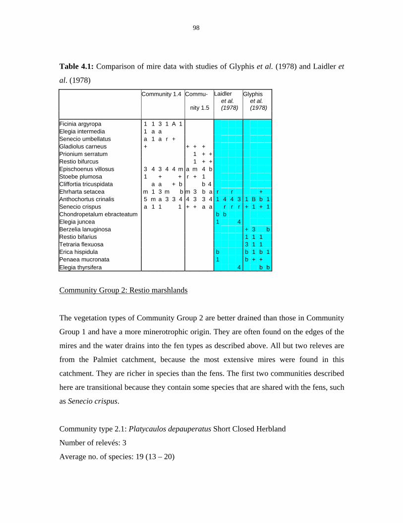
98
Table 4.1: Comparison of mire data with studies of Glyphis et al. (1978) and Laidler et
al. (1978)
Community 1.4 Commu- Laidler Glyphis
nity 1.5 et al. (1978)
et al. (1978)
Ficinia argyropa 1 1 3 1 A 1 Elegia intermedia 1 a a Senecio umbellatus a 1 a r + Gladiolus carneus + + + + Prionium serratum 1 + + Restio bifurcus 1 + + Epischoenus villosus 3 4 3 4 4 m a m 4 b Stoebe plumosa 1 + + r + 1 Cliffortia tricuspidata a a + b b 4 Ehrharta setacea m 1 3 m b m 3 b a r r + Anthochortus crinalis 5 m a 3 3 4 4 3 3 4 1 4 4 3 1 B b 1Senecio crispus a 1 1 1 + + a a r r r + 1 + 1Chondropetalum ebracteatum b b Elegia juncea 1 4 Berzelia lanuginosa + 3 bRestio bifarius 1 1 1 Tetraria flexuosa 3 1 1 Erica hispidula b b 1 b 1Penaea mucronata 1 b + + Elegia thyrsifera 4 b b
Community Group 2: Restio marshlands
The vegetation types of Community Group 2 are better drained than those in Community
Group 1 and have a more minerotrophic origin. They are often found on the edges of the
mires and the water drains into the fen types as described above. All but two releves are
from the Palmiet catchment, because the most extensive mires were found in this
catchment. They are richer in species than the fens. The first two communities described
here are transitional because they contain some species that are shared with the fens, such
as Senecio crispus.
Community type 2.1: Platycaulos depauperatus Short Closed Herbland
Number of relevés: 3
Average no. of species: 19 (13 – 20)
99
This is the only seepage type that is dominated by the restio Platycaulos depauperatus,
which forms dense green mats and is the most conspicuous differential species of this
community. It occurs together with the tussock-forming Restio subtilis, which is co-
dominant. Together they form the dominant lower herb stratum. One emergent species,
Chondropetalum mucronatum, 1.5 m tall, forms its own stratum. The species Elegia
neesii, Epischoenus villosus and Tetraria capillacea are all significantly lower. In
addition to the dominant species, additional differential species of this community are the
grass Pentameris hirtiglumis and the geophyte Kniphofia tabularis, that only flowers
after a fire. Although this community is undersampled because of the fire and is
described here on the basis of three samples, I can conclude from observations prior to
the fire that it is quite common in the Palmiet River catchment. It seems to be
intermediate between the Ficinio argyropae-Epischoenetum villosi from peaty soils and
the Tetrario capillaceae-Restionetum subtilis from more minerotrophic soils. It receives
less rainfall than other seepage types, with a Mean Annual Precipitation of just over 2000
mm.
Community type 2.2: Erica autumnalis-Restio purpurascens Tall Closed Restioland
Number of relevés: 2
Range of species number: 19 – 38
This is one of the two communities described from riparian mires. These communities
occur in the highest reaches of the rivers (in this study all were sampled in the Palmiet
River catchment) and are a mixture of seepage and riparian elements. Together they
make up the most species-rich communities, either in comparison to other seepage types
or to the riparian communities. This community has a more prominent tall herb layer than
most seepage communities. The dominant species is Restio purpurascens, but Elegia
racemosa and E. thyrsifera are also abundant. In the lower stratum Anthochortus crinalis
is a conspicuous species. Some species such as Hippia pilosa and Senecio crispus are
shared with Community Group 1. This type can best be described as a Restioland,
because small and big restio species are the most important constituents of this
community. It is difficult to determine the differential species in a situation where relevés
100
are few, but possible differential species are Aristea bakeri, Cliffortia ovalis, Elegia
racemosa, Hippia pilosa and an unidentified species of Asteraceae. The differential
species Erica autumnalis, which is used in the provisional name, is endemic to the
Hottentots Holland Mountains. The community occurs in the highest reaches of the
Wesselsgat River where riverbanks are steep and rocky.
Community type 2.3: Grubbia rosmarinifolia-Restio aff. versatilis Medium Closed
Shrubland
Number of relevés: 3
Average no. of species: 25 (18 – 33)
This is the second type of riparian seepages found along high altitude streams. The main
difference from the previous type is the shape of the banks, which are flatter and less
rocky in this vegetation. The dominant small restio here is Restio aff. versatilis,
compared to Anthochortus crinalis in the previous type.
This community has a more prominent tall herb stratum than most other seepage
types and the tall vegetation (between 1 and 1.5 metres) is dominated by the shrubs
Berzelia squarrosa, Brunia alopecuroides and Grubbia rosmarinifolia and the restioids
Restio purpurascens and Chondropetalum mucronatum. The most closely related riparian
community is the Erico-Tetrarietum crassae (see Chapter 5) which shares many Erica-
species with the Grubbia rosmarinifolia-Restio aff. versatilis Closed Shrubland. The
most closely related seepage community is the Tetrario capillaceae-Restionetum subtilis.
Restio aff. versatilis, a species that is dominant in the ground layer, is shared with this
community. The Grubbia rosmarinifolia-Restio aff. versatilis Community is typical of
situations where the riverbanks are not steep and there is a lot of lateral seepage. It can be
described as a shrubland because of the high cover of Ericaceae and Bruniaceae. There
are numerous differential species in this community, most of which are shared with
Ericaceous Fynbos and Erico-Tetrarietum crassae in particular. They are, amongst
others, Berzelia squarrosa, Brunia alopecuroides, Erica fastigiata, Grubbia
rosmarinifolia and Restio bifidus.

101
Community type 2.4: Tetraria capillacea-Restio subtilis Short to Tall Closed Restioland
Scientific name: Tetrario capillaceae-Restionetum subtilis ass. nova hoc loco
Type relevé: 86 (Appendix E; Table 1)
Number of relevés: 9
Average no. of species: 15 (10 – 17)
This is the most common type of seepage in the area, which is characterised by
the absence of Senecio crispus. The dominant restio is Restio subtilis, with Anthochortus
crinalis and Restio aff. versatilis as co-dominants. A typical characteristic is the mosaic
between the low vegetation formed by the small restios and sedges (Restio subtilis, R. aff.
versatilis, Tetraria capillacea and Epischoenus villosus) and the tall vegetation
consisting only of Chondropetalum mucronatum. This species does not resprout after
fires, like many other seepage species, but regenerates from seed. It tends to dominate the
community because the old plants form a thick litter layer on the soil beneath it, which
seems to prohibit other (aggressively spreading) clonal species from growing there.
Differential species of this community are few, because most species are shared with the
Grubbia rosmarinifolia-Restio aff. versatilis Closed Shrubland. Diagnostic features are
mostly the dominance of Restio subtilis and the occurrence of Chrysithrix species. As in
the case of the riparian seepage types, this community contains numerous shrub species,
such as the differential species Grubbia rosmarinifolia and Berzelia squarrosa, but they
do not grow very tall.
This community occurs on more minerotrophic soils than the former
communities. Nevertheless, the soils are very acidic and highly organic. In one case it
was found in a riparian zone and it is closely related to the riparian seepage types
described above. The community described by Boucher (1978) as Chondropetalum-
Restio Tussock Marsh seems to be quite similar, but the dominant small Restio in the
Kogelberg is not Restio subtilis but Restio ambiguus and many other species are absent in
the Kogelberg community.
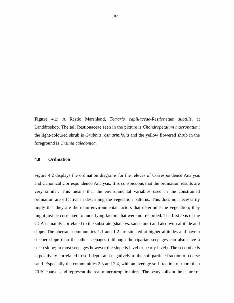
102
Figure 4.1: A Restio Marshland, Tetrario capillaceae-Restionetum subtilis, at
Landdroskop. The tall Restionaceae seen in the picture is Chondropetalum mucronatum;
the light-coloured shrub is Grubbia rosmarinifolia and the yellow flowered shrub in the
foreground is Ursinia caledonica.
4.8 Ordination
Figure 4.2 displays the ordination diagrams for the relevés of Correspondence Analysis
and Canonical Correspondence Analysis. It is conspicuous that the ordination results are
very similar. This means that the environmental variables used in the constrained
ordination are effective in describing the vegetation patterns. This does not necessarily
imply that they are the main environmental factors that determine the vegetation; they
might just be correlated to underlying factors that were not recorded. The first axis of the
CCA is mainly correlated to the substrate (shale vs. sandstone) and also with altitude and
slope. The aberrant communities 1.1 and 1.2 are situated at higher altitudes and have a
steeper slope than the other seepages (although the riparian seepages can also have a
steep slope; in most seepages however the slope is level or nearly level). The second axis
is positively correlated to soil depth and negatively to the soil particle fraction of coarse
sand. Especially the communities 2.3 and 2.4, with an average soil fraction of more than
20 % coarse sand represent the real minerotrophic mires. The peaty soils in the centre of
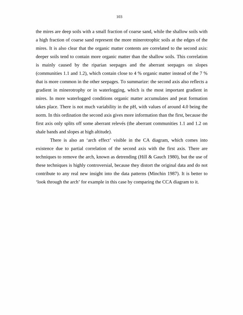
103
the mires are deep soils with a small fraction of coarse sand, while the shallow soils with
a high fraction of coarse sand represent the more minerotrophic soils at the edges of the
mires. It is also clear that the organic matter contents are correlated to the second axis:
deeper soils tend to contain more organic matter than the shallow soils. This correlation
is mainly caused by the riparian seepages and the aberrant seepages on slopes
(communities 1.1 and 1.2), which contain close to 4 % organic matter instead of the 7 %
that is more common in the other seepages. To summarize: the second axis also reflects a
gradient in minerotrophy or in waterlogging, which is the most important gradient in
mires. In more waterlogged conditions organic matter accumulates and peat formation
takes place. There is not much variability in the pH, with values of around 4.0 being the
norm. In this ordination the second axis gives more information than the first, because the
first axis only splits off some aberrant relevés (the aberrant communities 1.1 and 1.2 on
shale bands and slopes at high altitude).
There is also an ‘arch effect’ visible in the CA diagram, which comes into
existence due to partial correlation of the second axis with the first axis. There are
techniques to remove the arch, known as detrending (Hill & Gauch 1980), but the use of
these techniques is highly controversial, because they distort the original data and do not
contribute to any real new insight into the data patterns (Minchin 1987). It is better to
‘look through the arch’ for example in this case by comparing the CCA diagram to it.
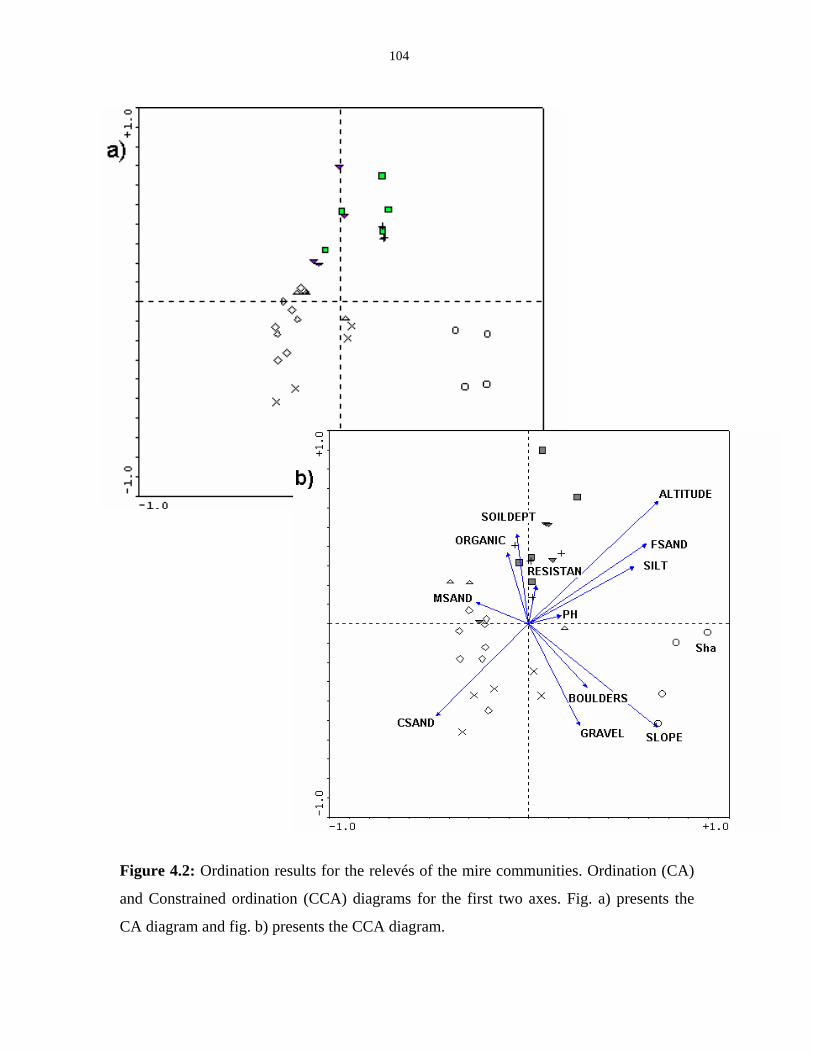
104
Figure 4.2: Ordination results for the relevés of the mire communities. Ordination (CA)
and Constrained ordination (CCA) diagrams for the first two axes. Fig. a) presents the
CA diagram and fig. b) presents the CCA diagram.
105
4.9 Undersampled communities
The fynbos has an extremely high species turnover between mountain ranges (Kruger &
Taylor 1979; Cowling et al. 1992) and this might be most applicable to the high altitudes
because mountain tops have a high insular effect. Campbell (1986b) describes the
Sneeukop Azonal Restioid Fynbos specifically for the ‘Wet’ Mountain Ranges like Table
Mountain, the Kogelberg and the Hottentots Holland Mountains. Because of these
assumptions, the question arose as to the extent of species turnover in seepage
communities is and therefore whether the classification proposed here was also
applicable to nearby mountain ranges. For this purpose, six additional seepage relevés
were sampled in nearby mountain ranges. These were recorded from the Akkedisberg
(16th degree square map 3419 BC), the Dutoitskloof (16th degree square map 3319 CA)
and the Groenland Mountains (16th degree square map 3419 AA). Two out of the six
additional relevés (both from Dutoitskloof) fitted well into the classification for the
Hottentots Holland Mountains: relevé 259 was classified as Ficinio argyropae-
Epischoenetum villosi and relevé 262 fitted into the Tetrario capillaceae-Restietum
subtilis, although it is slightly different. The other four relevés emerged as outliers in the
classification and ordination for the Hottentots Holland Mountains which shows that
there are many vegetation types yet to be described from these habitats. The relevés that
did not fit will be described below.
Community type 3.1: Isolepis prolifer-Bulbinella nutans Tall Closed Sedgeland
This community was found in the Dutoitskloof Mountains and is completely different
from any community in the Hottentots Holland Mountains. It occurs in a very wet
habitat: the watertable is exposed above the ground. A similar habitat was not found in
the Hottentots Holland Mountains. The species with their respective cover values,
arranged according to importance are: Bulbinella nutans (5), Isolepis prolifer (3), Elegia
thyrsifera (2b) and Sphagnum capense (1).
Community type 3.2: Anthochortus crinalis-Restio brachiatus Tall Closed Restioland
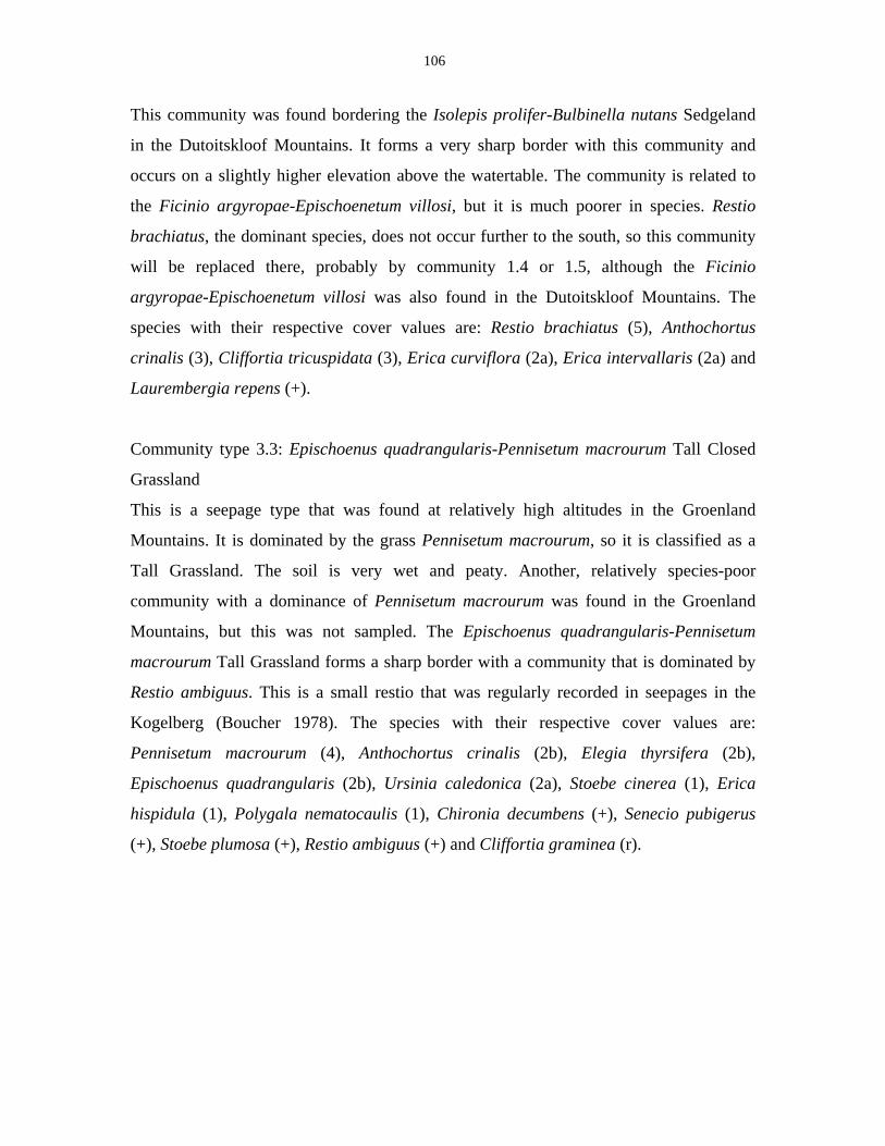
106
This community was found bordering the Isolepis prolifer-Bulbinella nutans Sedgeland
in the Dutoitskloof Mountains. It forms a very sharp border with this community and
occurs on a slightly higher elevation above the watertable. The community is related to
the Ficinio argyropae-Epischoenetum villosi, but it is much poorer in species. Restio
brachiatus, the dominant species, does not occur further to the south, so this community
will be replaced there, probably by community 1.4 or 1.5, although the Ficinio
argyropae-Epischoenetum villosi was also found in the Dutoitskloof Mountains. The
species with their respective cover values are: Restio brachiatus (5), Anthochortus
crinalis (3), Cliffortia tricuspidata (3), Erica curviflora (2a), Erica intervallaris (2a) and
Laurembergia repens (+).
Community type 3.3: Epischoenus quadrangularis-Pennisetum macrourum Tall Closed
Grassland
This is a seepage type that was found at relatively high altitudes in the Groenland
Mountains. It is dominated by the grass Pennisetum macrourum, so it is classified as a
Tall Grassland. The soil is very wet and peaty. Another, relatively species-poor
community with a dominance of Pennisetum macrourum was found in the Groenland
Mountains, but this was not sampled. The Epischoenus quadrangularis-Pennisetum
macrourum Tall Grassland forms a sharp border with a community that is dominated by
Restio ambiguus. This is a small restio that was regularly recorded in seepages in the
Kogelberg (Boucher 1978). The species with their respective cover values are:
Pennisetum macrourum (4), Anthochortus crinalis (2b), Elegia thyrsifera (2b),
Epischoenus quadrangularis (2b), Ursinia caledonica (2a), Stoebe cinerea (1), Erica
hispidula (1), Polygala nematocaulis (1), Chironia decumbens (+), Senecio pubigerus
(+), Stoebe plumosa (+), Restio ambiguus (+) and Cliffortia graminea (r).
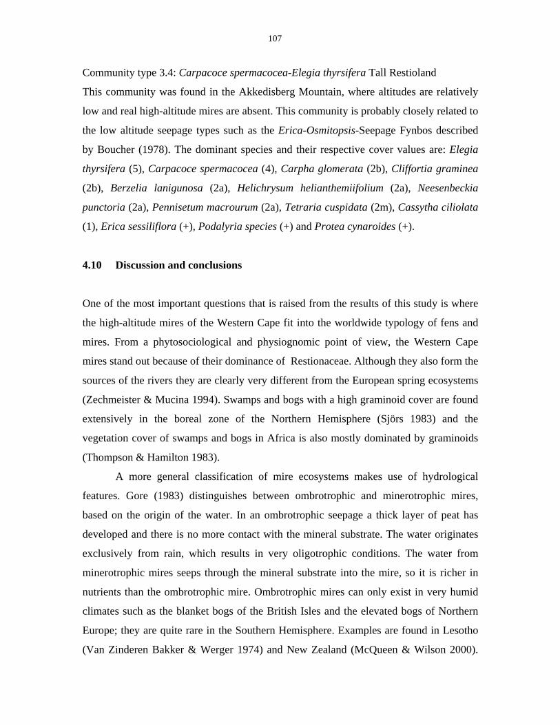
107
Community type 3.4: Carpacoce spermacocea-Elegia thyrsifera Tall Restioland
This community was found in the Akkedisberg Mountain, where altitudes are relatively
low and real high-altitude mires are absent. This community is probably closely related to
the low altitude seepage types such as the Erica-Osmitopsis-Seepage Fynbos described
by Boucher (1978). The dominant species and their respective cover values are: Elegia
thyrsifera (5), Carpacoce spermacocea (4), Carpha glomerata (2b), Cliffortia graminea
(2b), Berzelia lanigunosa (2a), Helichrysum helianthemiifolium (2a), Neesenbeckia
punctoria (2a), Pennisetum macrourum (2a), Tetraria cuspidata (2m), Cassytha ciliolata
(1), Erica sessiliflora (+), Podalyria species (+) and Protea cynaroides (+).
4.10 Discussion and conclusions
One of the most important questions that is raised from the results of this study is where
the high-altitude mires of the Western Cape fit into the worldwide typology of fens and
mires. From a phytosociological and physiognomic point of view, the Western Cape
mires stand out because of their dominance of Restionaceae. Although they also form the
sources of the rivers they are clearly very different from the European spring ecosystems
(Zechmeister & Mucina 1994). Swamps and bogs with a high graminoid cover are found
extensively in the boreal zone of the Northern Hemisphere (Sjörs 1983) and the
vegetation cover of swamps and bogs in Africa is also mostly dominated by graminoids
(Thompson & Hamilton 1983).
A more general classification of mire ecosystems makes use of hydrological
features. Gore (1983) distinguishes between ombrotrophic and minerotrophic mires,
based on the origin of the water. In an ombrotrophic seepage a thick layer of peat has
developed and there is no more contact with the mineral substrate. The water originates
exclusively from rain, which results in very oligotrophic conditions. The water from
minerotrophic mires seeps through the mineral substrate into the mire, so it is richer in
nutrients than the ombrotrophic mire. Ombrotrophic mires can only exist in very humid
climates such as the blanket bogs of the British Isles and the elevated bogs of Northern
Europe; they are quite rare in the Southern Hemisphere. Examples are found in Lesotho
(Van Zinderen Bakker & Werger 1974) and New Zealand (McQueen & Wilson 2000).
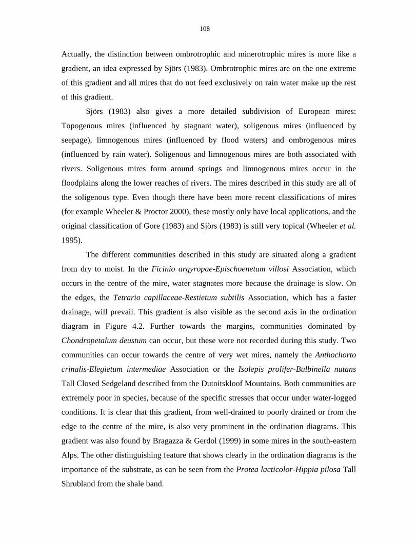
108
Actually, the distinction between ombrotrophic and minerotrophic mires is more like a
gradient, an idea expressed by Sjörs (1983). Ombrotrophic mires are on the one extreme
of this gradient and all mires that do not feed exclusively on rain water make up the rest
of this gradient.
Sjörs (1983) also gives a more detailed subdivision of European mires:
Topogenous mires (influenced by stagnant water), soligenous mires (influenced by
seepage), limnogenous mires (influenced by flood waters) and ombrogenous mires
(influenced by rain water). Soligenous and limnogenous mires are both associated with
rivers. Soligenous mires form around springs and limnogenous mires occur in the
floodplains along the lower reaches of rivers. The mires described in this study are all of
the soligenous type. Even though there have been more recent classifications of mires
(for example Wheeler & Proctor 2000), these mostly only have local applications, and the
original classification of Gore (1983) and Sjörs (1983) is still very topical (Wheeler et al.
1995).
The different communities described in this study are situated along a gradient
from dry to moist. In the Ficinio argyropae-Epischoenetum villosi Association, which
occurs in the centre of the mire, water stagnates more because the drainage is slow. On
the edges, the Tetrario capillaceae-Restietum subtilis Association, which has a faster
drainage, will prevail. This gradient is also visible as the second axis in the ordination
diagram in Figure 4.2. Further towards the margins, communities dominated by
Chondropetalum deustum can occur, but these were not recorded during this study. Two
communities can occur towards the centre of very wet mires, namely the Anthochorto
crinalis-Elegietum intermediae Association or the Isolepis prolifer-Bulbinella nutans
Tall Closed Sedgeland described from the Dutoitskloof Mountains. Both communities are
extremely poor in species, because of the specific stresses that occur under water-logged
conditions. It is clear that this gradient, from well-drained to poorly drained or from the
edge to the centre of the mire, is also very prominent in the ordination diagrams. This
gradient was also found by Bragazza & Gerdol (1999) in some mires in the south-eastern
Alps. The other distinguishing feature that shows clearly in the ordination diagrams is the
importance of the substrate, as can be seen from the Protea lacticolor-Hippia pilosa Tall
Shrubland from the shale band.
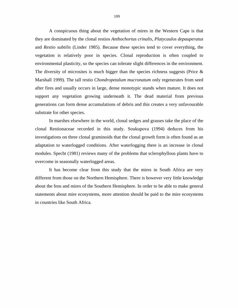
109
A conspicuous thing about the vegetation of mires in the Western Cape is that
they are dominated by the clonal restios Anthochortus crinalis, Platycaulos depauperatus
and Restio subtilis (Linder 1985). Because these species tend to cover everything, the
vegetation is relatively poor in species. Clonal reproduction is often coupled to
environmental plasticity, so the species can tolerate slight differences in the environment.
The diversity of microsites is much bigger than the species richness suggests (Price &
Marshall 1999). The tall restio Chondropetalum mucronatum only regenerates from seed
after fires and usually occurs in large, dense monotypic stands when mature. It does not
support any vegetation growing underneath it. The dead material from previous
generations can form dense accumulations of debris and this creates a very unfavourable
substrate for other species.
In marshes elsewhere in the world, clonal sedges and grasses take the place of the
clonal Restionaceae recorded in this study. Soukupova (1994) deduces from his
investigations on three clonal graminoids that the clonal growth form is often found as an
adaptation to waterlogged conditions. After waterlogging there is an increase in clonal
modules. Specht (1981) reviews many of the problems that sclerophyllous plants have to
overcome in seasonally waterlogged areas.
It has become clear from this study that the mires in South Africa are very
different from those on the Northern Hemisphere. There is however very little knowledge
about the fens and mires of the Southern Hemisphere. In order to be able to make general
statements about mire ecosystems, more attention should be paid to the mire ecosystems
in countries like South Africa.
110
5. Description of the riparian vegetation types of the Hottentots Holland
Mountains
5.1 Abstract
This paper presents the results of a Braun-Blanquet phytosociological survey of the
riparian vegetation of the mountain streams in the Hottentots Holland Mountains. For the
purposes of this study, the riparian vegetation is subdivided into the following zones: the
Wet Bank, Lower Dynamic, Shrub/Tree and Back Dynamic Zones. The vegetation is
sampled along transects in which each riparian zone is sampled separately. The
vegetation data are analysed using a combination of TWINSPAN followed by manual
tabulation using the Megatab computer program. Twenty-six riparian plant communities
are described which vary structurally from sparse sedgelands and tall fynbos to scrub and
forest. The most important factor that explains the vegetation patterns is the inundation
frequency, which is, however, difficult to quantify in mountain streams. The investigation
of the inundation frequency is described in a separate study (Sieben et al., Chapter 6).
Each catchment has unique features that are reflected by differences in the vegetation.
Communities located on the shales and granites are, for instance, quite distinct from
those on the sandstones, while altitude also plays a major role in determining community
composition.
5.2 Introduction
Except for the floristic diversity of the fynbos, the mountains of the Western Cape are
valued for the high quality drinking water they produce (King & Day 1979). This aspect
will continue to play a bigger role as the population of the Cape Metropolitan Area grows
and the water demand continues to increase (Davies & Day 1998). The majority of the
rivers nowadays are dammed in at least one place and few rivers experience natural flood
regimes. It is only in the higher reaches of the rivers where the riparian vegetation still
111
occurs in a more or less natural state (King & Day 1979) and it is this vegetation that
forms the subject of this chapter.
Riparian vegetation plays a very important role in the functioning of a riverine
ecosystem. It prohibits erosion, slows down turbulent floods, consumes water and adds to
species and habitat diversity (Kopecky 1963; Rogers & Van der Zel 1989; Birkhead et al.
1996). Anthropogenic threats to riparian vegetation are caused mainly by alien vegetation
and modified flood regimes. Many studies have paid attention to the changes in riparian
vegetation after the flood regime has been altered (Franz & Bazzaz 1977; Johnson et al.
1995; Stevens et al. 1995; Marston et al. 1995; Tremolières et al. 1998). Most of these
studies have focussed on the lower reaches of rivers and the upper reaches have generally
been ignored, however, in mountain streams there is also an obvious relationship between
flooding and vegetation patterns.
Different authors write about the zonation patterns that occur along rivers, but no
agreement has been achieved yet on a standard terminology to apply to the zones
(Kopecky 1969; Menges & Waller 1983; Hupp & Osterkamp 1985; Bowman &
McDonough 1991; Glavaç et al. 1992; Dixon & Johnson 1999; Boucher & Tlale 1999).
Kopecky (1969) is the first author to subdivide the riparian banks into different ecotopes:
the submerse, demerse, semimerse and emerse ecotopes. The criterium used to subdivide
the banks is the flood regime. Later on, Menges & Waller (1983) proposed a subdivision
based on the life strategies of the plants growing in the zones. It is important to make a
distinction between different geomorphic types of riverbanks, such as a floodplain
(Menges & Waller 1983) and a steep riverbank (Dixon & Johnson 1999; Boucher &
Tlale 1999). Kopecky (1969) also recognized this and treated the eurysaleutic bank type
(that of the lower reaches of the rivers, with gentle bank slopes and high floods)
differently from the stenosaleutic bank type (that of the higher reaches of the rivers, with
steep bank slopes and low floods). His subdivision has an advantage over that of Menges
& Waller (1983), in that it is based on fluvial processes so that it can be used as a more
generic subdivision and be extrapolated to different biomes.
The subdivision used by Boucher & Tlale (1999) is based partly on the fluvial
processes and partly on the structure of the vegetation. This has the advantage that it is
easily applied in the field. Their Aquatic Zone is the same as Kopecky’s (1969) submerse
112
ecotope, their Wetbank Zone equates to the demerse ecotope, the Lower Dynamic Zone
to the semimerse ecotope and the Back Dynamic Zone to the emerse ecotope.
Additionally, Boucher & Tlale (1999) recognize a Shrub/Tree Zone between the Lower-
and Back Dynamic Zones. This Shrub/Tree zone can be recognized in many riverine
ecosystems worldwide and also plays a distinct role in the fluvial processes. It slows
down floods, so that deposition of sediments takes place, and is a source of woody debris
(Fetherston et al. 1995). The subdivisions of Boucher & Tlale (1999) are used in this
study because of their applicability.
This study aims at describing the vegetation types of the riparian habitats in the
Hottentots Holland Mountains in the Western Cape and the ecological processes that
drive them.
5.3 Study area
The area chosen to undertake a detailed study of mountain riparian vegetation of the
Western Cape, is the Hottentots Holland Nature Reserve, which is situated between
Stellenbosch, Franschhoek, Somerset West and Grabouw. It has the highest rainfall in the
entire Western Cape. Five different rivers originate here: 1.) The Berg River, a major
river that flows north through the West Coast forelands; 2.) the Riviersonderend River,
another major river that flows east through the Overberg Region, and joins the Breede
River near Swellendam; 3.) the Palmiet River, an intermediate sized river that flows
through the Kogelberg State Forest towards the south; 4.) the Eerste River, a small river
that flows west through Stellenbosch towards the False Bay coast and 5.) the Lourens
River, a small south-west flowing river that flows directly to the False Bay coast through
Somerset West. Out of these five rivers, only the Riviersonderend, through the Breede
River, flows into the Indian Ocean. The four other rivers flow into the Atlantic Ocean.
The Hottentots Holland Nature Reserve is situated in the core area of species
richness of the Fynbos Biome (Boucher 1978; Cowling et al. 1992). Because of the high
rainfall, the high diversity of plant species and the high diversity in habitats, the area was
considered to be an ideal location for a first detailed study of mountain riparian
113
vegetation in the region, to provide a maximum amount of information about riparian
habitats. 5.4 Soils and pedogenesis
The soils adjacent to mountain streams are poorly developed and contain a high
proportion of rocks. In many instances the topsoil is completely washed away and the
banks consist entirely of bedrock, boulders and large cobbles. The best developed soils
are found in the Back Dynamic Zone. The deepest soils that can be found along the rivers
are in the forests, the shale-bands and in seepage areas or floodplains. Fry (1987)
describes the catenas (soil gradients) that occur on the slopes of Swartboschkloof in the
Eerste River catchment. The soils at the bases of these catenas can be found in the Back
Dynamic Zones of the rivers. This is mainly the Mispah Form on sandstone or granite
substrates. In some places on shale bands and granite substrates, the red apedal soils of
the Glenrosa Form can be found in the riparian zone. Under forests, the brown humic
soils of the Oakleaf Form can be found. In lowlands and depressions, where small
floodplains are formed, the Fernwood Form occurs. This Form belongs to the group of
pale soils and it occurs in two phases: the wet form occurs where hydromorphic
processes dominate and the dry form where podzolisation dominates. Another soil form
that is associated with rivers but that was not found in the present study is the Dundee
Form (Kruger 1974).
5.5 River ecology
Rivers are very complex ecosystems that reflect the environmental situation in the entire
catchment. The climate and the geological substrate in a subcatchment of a river have an
impact on the riverine ecosystem, the runoff and the water quality (Boucher & Marais
1993). Any human activity in the catchment will also affect the river downstream. For
example, Dye (1996) has shown that pine plantations in a subcatchment decrease the
runoff because a plantation uses more water than indigenous vegetation. However, rivers
114
are resilient systems and the impact of a disturbance decreases with increasing distance
downstream (Ward & Stanford 1979).
The catchment is not a fixed network of river channels, but a dynamic expanding
or shrinking source area (Hewlett 1961; Hewlett & Hibbert 1967). Some water is stored
in the soil while rivers depend on a restricted source area for their water supply. The
course that water follows before it enters the river will have a great impact on the water
quality in the river. For example, if water percolates through an agricultural area, the
water flowing in the river will be enriched in nutrients, while the runoff from an
undisturbed area where sandstones dominate, the substrate will be very poor in nutrients
(Bosch et al. 1986). In the Fynbos Biome, runoff yields between 35 – 55% of the total
rainfall. This value is high compared to other biomes in South Africa. After a fire, runoff
increases even more and only returns to its original level after about 15 years (Cowling et
al. 1997).
Mountain streams, which form the subject of this study, have some characteristics
that make them different from the lower reaches of rivers. In mountain streams erosion is
dominant over deposition. This creates a very unstable substrate both in the riverbed and
on the banks. Organisms living in the streams, whether they are plants or animals, are
few but are highly adapted (Davies & Day 1998). The riverine ecosystem here stands out
because it is entirely dependent on an external food source: the litter from the riparian
vegetation. The interaction between shredder populations and the input of allochthonous
plant material play a major role in these ecosystems (King 1981; Stewart & Davies 1990;
Stewart 1992).
Some reviews of ecological processes taking place in Southern African riverine
ecosystems are presented by Davies & Day (1989, 1998) and Day et al. (1986).
5.6 Vegetation types
Accounts of Western Cape riverine vegetation types are mainly rather general, such as
those by Taylor (1978), Kruger (1978b) and Campbell (1986b), while Werger et al.
(1972), Campbell & Moll (1977), Boucher (1978) and McDonald (1988) offer detailed
vegetation descriptions of specific areas. Kruger (1978b) also gives a detailed account of
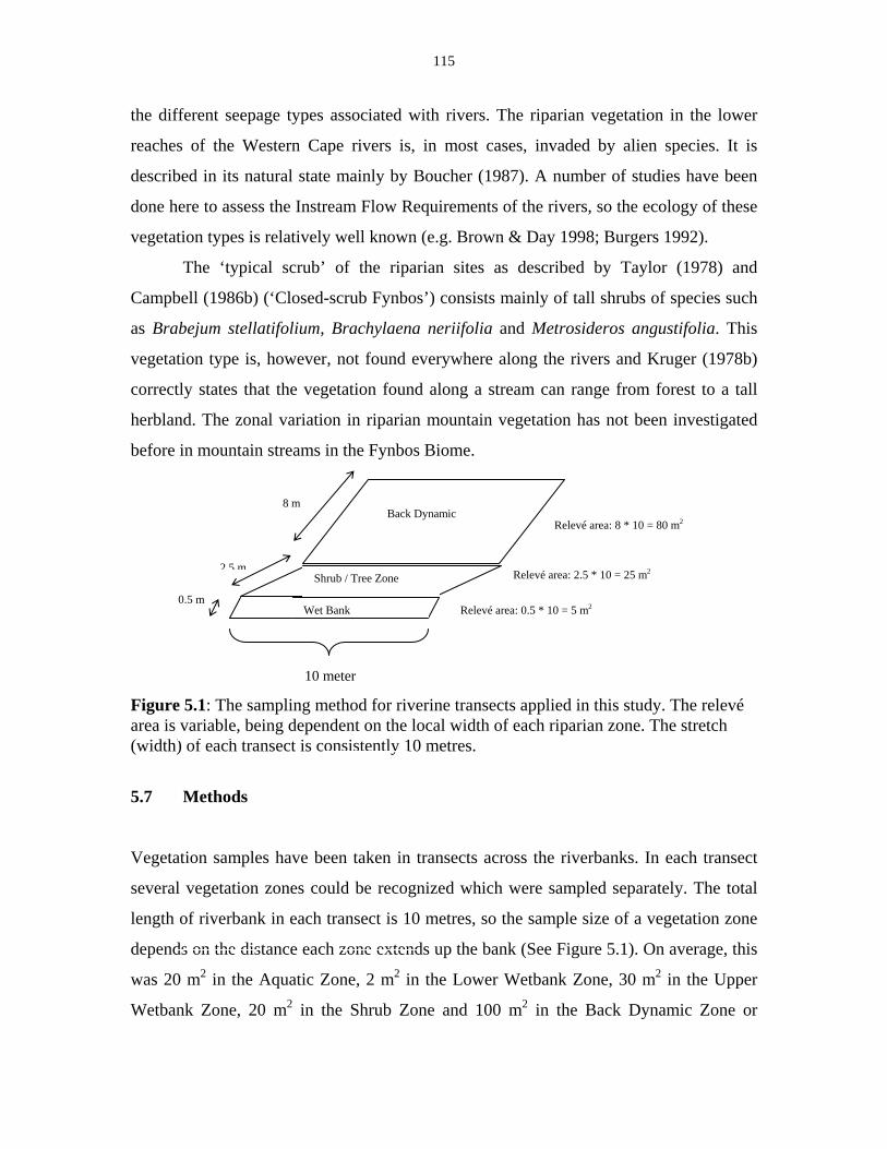
115
the different seepage types associated with rivers. The riparian vegetation in the lower
reaches of the Western Cape rivers is, in most cases, invaded by alien species. It is
described in its natural state mainly by Boucher (1987). A number of studies have been
done here to assess the Instream Flow Requirements of the rivers, so the ecology of these
vegetation types is relatively well known (e.g. Brown & Day 1998; Burgers 1992).
The ‘typical scrub’ of the riparian sites as described by Taylor (1978) and
Campbell (1986b) (‘Closed-scrub Fynbos’) consists mainly of tall shrubs of species such
as Brabejum stellatifolium, Brachylaena neriifolia and Metrosideros angustifolia. This
vegetation type is, however, not found everywhere along the rivers and Kruger (1978b)
correctly states that the vegetation found along a stream can range from forest to a tall
herbland. The zonal variation in riparian mountain vegetation has not been investigated
before in mountain streams in the Fynbos Biome.
Figure 5.1: The sampling method for riverine transects applied in this study. The relevé area is variable, being dependent on the local width of each riparian zone. The stretch (width) of each transect is consistently 10 metres.
5.7 Methods
Vegetation samples have been taken in transects across the riverbanks. In each transect
several vegetation zones could be recognized which were sampled separately. The total
length of riverbank in each transect is 10 metres, so the sample size of a vegetation zone
depends on the distance each zone extends up the bank (See Figure 5.1). On average, this
was 20 m2 in the Aquatic Zone, 2 m2 in the Lower Wetbank Zone, 30 m2 in the Upper
Wetbank Zone, 20 m2 in the Shrub Zone and 100 m2 in the Back Dynamic Zone or
8 m
0.5 m
2 5 m
10 meter
Wet Bank
Shrub / Tree Zone
Back Dynamic
Relevé area: 0.5 * 10 = 5 m2
Relevé area: 2.5 * 10 = 25 m2
Relevé area: 8 * 10 = 80 m2
116
riparian forest. These sample sizes comply well with the sample sizes recommended by
Tüxen (1970) for the different structural vegetation types involved (see also Westhoff &
Van der Maarel 1973). Vegetation sampling followed the Braun-Blanquet Method
(Westhoff & Van der Maarel 1973; Werger 1974). Glavaç et al. (1992) pay attention to
the nature of vegetation borders along a riparian gradient; they found that even along a
continuous gradient several homogeneous vegetation units could be recognized.
Vegetation sampling in transects is thus quite feasible, because the different zones are
well defined and easily recognizable.
TWINSPAN and manual tabulation (Hill 1979) are used to classify the vegetation
samples. When undertaking manual tabulation, the vegetation scientist assesses the
acceptability of the TWINSPAN components in groups and uses his knowledge of the
vegetation in the field and of the particular sites as a reference. The aim of reshuffling is
to cluster the presence and absence of species as far as possible into blocks (Feoli &
Orloci 1983). The programme used for this purpose is Megatab (Hennekens 1996). The
clusters that are sufficiently sampled have been given scientific names according to the
International Code of Syntaxonomic Nomenclature of Weber et al. (2000). Community
names for local use (for example by managers) are based on the vegetation structure and
two names of important species (Edwards 1983). These names have been given to all the
communities described. The hierarchical relationships between communities have been
examined using the program SYNTAX (Podani 1994).
For the gradient analysis of the vegetation, using multivariate techniques, there
are two different methods available, namely, ordination (direct gradient analysis) and
constrained ordination (indirect gradient analysis). The program package Canoco 4 is
used here for these analyses (Ter Braak & Šmilauer 1998). The compositional data such
as particle sizes have been log-transformed prior to further analysis, according to the
recommendations of Ter Braak & Šmilauer (1998). The technique used for indirect
gradient analysis is Correspondence Analysis (CA), which makes use of the Weighted
Averaging algorithm applicable for unimodal response curves (Hill 1974). Økland (1996)
argues that CA and Canonical Correspondence Analysis (CCA) should be used
complementarily because CCA does not account for the variation that is explained by
variables that were not recorded. If the results of CA and CCA are very similar it is clear
117
that all the important environmental variables were included in the study. In this study,
only a CA is carried out, while the constrained ordinations are dealt with in more detail in
Chapter 7.
5.8 Results
Twenty-six riparian communities have been recognized together with five
subcommunities. The dendrogram showing the hierarchical relationships between the
different communities resulting from the analysis in SYNTAX, is presented in Figure 5.2.
This dendrogram, together with the CA ordination diagram of Figure 5.3, is used to study
and interpret the relationships and the transitions between the different vegetation types
described in this study. The vegetation units that are closely related can be found near
each other in both the dendrogram and the ordination diagram. There is insufficient data
from similar communities in other parts of the Fynbos Biome, consequently this study
does not present a definitive hierarchical classification of the riparian vegetation types as
a whole. Communities are therefore only formally named at the level of the association
and below. Instead of a formal hierarchical classification, the vegetation units are
clustered into Community Groups, whose exact syntaxonomic status are not yet known.
Ten of these Community Groups have been recognized.
The riparian relevé data collected in this study are presented in five syntaxonomic
tables (Appendix E; Tables 2 to 6), each presenting one or more Community Groups, and
a synoptic table, which summarizes the information in the syntaxonomic tables
(Appendix E; Table 7). Thirty-one vegetation units are described. Scientific names are
given to 18 associations, eight subassociations and one alliance following Weber et al.
(2000). No scientific names are given to higher syntaxonomic units, because of a lack of
data. In cases where a syntaxonomic name is given, a type relevé is also indicated. The
differential species are listed together with the constant companions. These are defined
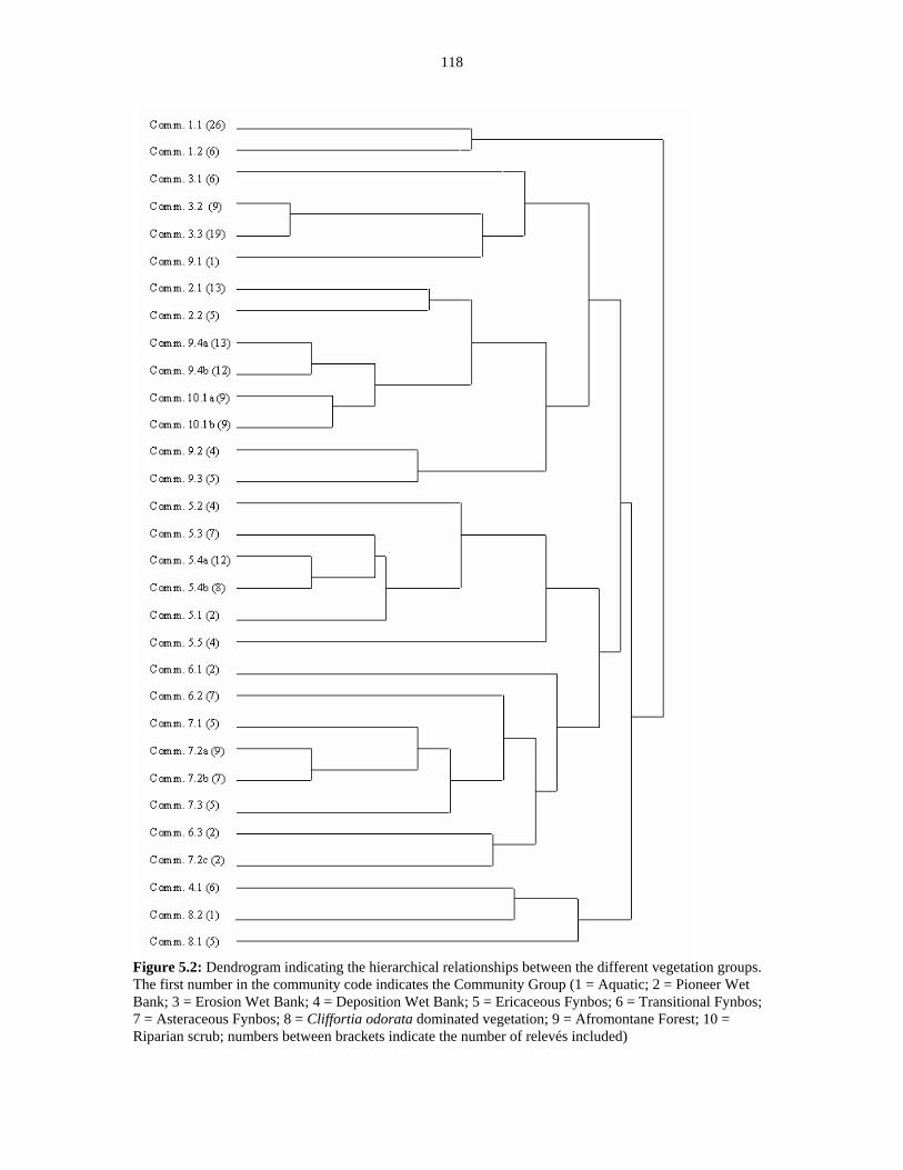
118
Figure 5.2: Dendrogram indicating the hierarchical relationships between the different vegetation groups. The first number in the community code indicates the Community Group (1 = Aquatic; 2 = Pioneer Wet Bank; 3 = Erosion Wet Bank; 4 = Deposition Wet Bank; 5 = Ericaceous Fynbos; 6 = Transitional Fynbos; 7 = Asteraceous Fynbos; 8 = Cliffortia odorata dominated vegetation; 9 = Afromontane Forest; 10 = Riparian scrub; numbers between brackets indicate the number of relevés included)
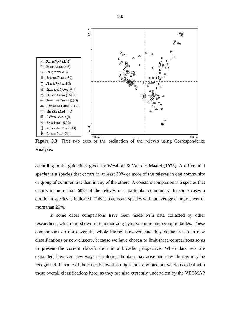
119
Figure 5.3: First two axes of the ordination of the relevés using Correspondence
Analysis.
according to the guidelines given by Westhoff & Van der Maarel (1973). A differential
species is a species that occurs in at least 30% or more of the relevés in one community
or group of communities than in any of the others. A constant companion is a species that
occurs in more than 60% of the relevés in a particular community. In some cases a
dominant species is indicated. This is a constant species with an average canopy cover of
more than 25%.
In some cases comparisons have been made with data collected by other
researchers, which are shown in summarizing syntaxonomic and synoptic tables. These
comparisons do not cover the whole biome, however, and they do not result in new
classifications or new clusters, because we have chosen to limit these comparisons so as
to present the current classification in a broader perspective. When data sets are
expanded, however, new ways of ordering the data may arise and new clusters may be
recognized. In some of the cases below this might look obvious, but we do not deal with
these overall classifications here, as they are also currently undertaken by the VEGMAP
120
project for which published and unpublished data from across the biome is currently
being collated (McDonald 1997; McDonald & Boucher 1999).
Aquatic communities (Appendix E; Table 2)
Community Group 1: Aquatic Communities
Aquatic communities in mountain streams must survive the stresses of high stream
velocities and dynamic substrates subject to rapid changes. These conditions inhibit the
roots, especially of the young seedlings, from taking a strong hold in the substrate.
Moreover, the rivers are often shaded by trees while the water is very poor in nutrients,
which is not conducive to rapid plant growth. Very few plants are suitably adapted to
survive these extreme conditions.
The aquatic communities are differentiated by two species: Isolepis digitata and
the exotic moss Fontinalis antipyretica. Isolepis digitata only occurs in places that
receive sufficient light. Where there is open water with a depth of up to one meter and
velocities are slow I. digitata can occur in high densities. Another aquatic moss, Wardia
hygrometrica, occurs in these rivers as well, although it was not recorded in the sample
sites. It is the only moss species endemic to the Fynbos Biome (King & Day 1979). Two
different communities are recognized, both described as associations. The two moss
species could be characteristic species, as Isolepis digitata occasionally also grows in the
Lower Wet Bank Zone. The two associations are combined into an alliance called
Isolepidion digitatae.
Community type 1.1: Isolepis digitata-Fontinalis antipyretica Community
Scientific name: Fontinali antipyreticae-Isolepidetum digitatae ass. nova hoc loco
Number of relevés: 26
Type relevé: 56 (Table 2)
Average no. of species: 2 (1 – 2)
This is an aquatic community dominated by Isolepis digitata and Fontinalis antipyretica.
The sedge Isolepis digitata covers, on average, 10% of each relevé while the moss
121
Fontinalis antipyretica covers less than 1% on average. Isolepis digitata mostly grows to
about 20 cm tall, but in deeper water it can grow taller. It prefers to grow on the
downstream side of the rocks where velocities are minimal. It will not grow taller than
the rock, so it will be protected when the river is in flood (pers. comm. G.R. Basson). The
community occurs is widespread in the mountain streams, with Isolepis digitata
dominating in places with heavy sunlight and Fontinalis antipyretica dominating in the
shady areas. The river bottom is covered by boulders between 0.25 m and 1.0 m in size.
In the mountain streams where this community occurs, depth is mostly shallow (on
average 0.2 m deep). In deeper water (up to 0.8 m) Isolepis digitata tends to have a high
percentage cover (over 50%).
Community type 1.2: Isolepis digitata-Pentaschistis pallida Community
Scientific name: Pentaschistido pallidae-Isolepidetum digitatae ass. nova hoc loco
Number of relevés: 6
Type relevé: 204 (Table 2)
Average no. of species: 3 (2 – 12)
This aquatic community occurs in places with shallow water, mostly on bedrock. Except
for the two differential species mentioned for the aquatic communities in general, this
community can be differentiated by a relatively high percentage cover of the grass
Pentaschistis pallida. This grass appears to have a broad ecological amplitude, because it
can also be found in some places in the Back Dynamic Zone. The dry patches within this
community support additional species, such as seedlings of different shrubs, ferns and
Wet Bank species such as Juncus lomatophyllus. There are also several species of mosses
and the liverwort Symphyogyna podophylla. Most of these species can be used to
differentiate this community from the Fontinali antipyreticae-Isolepidetum digitatae. In
places where there are many dry patches the community can become relatively species-
rich and this type (relevés 167, 204 and 205) is recognized as the ‘typical’ variant of the
Pentaschistido pallidae-Isolepidetum digitatae. This variant occurs in places with
bedrock and in waterfalls and vegetation cover is relatively high here (more than 50%).
The sedge Isolepis digitata is dominant. It makes up the greater part of the herb layer
122
which is 0.2 – 0.3 m tall. Mosses, of which Fontinalis antipyretica is the most important
species, also have a high cover. The other relevés (130, 132 and 250) are more
depauperate and belong to the ‘inops’-variant. Bedrock is sparser in this type and the
vegetation cover is also much lower.
Wet Bank communities (Appendix E; Table 3)
The Wet Bank Zones are the areas around the river that are flooded regularly. In some
cases, an Upper and a Lower Wet Bank can be distinguished but this is not always the
case.
Three completely different community groups occur in the Wet Bank Zone:
Erosion, Deposition and Pioneer Wetbanks. Few species are in common between these
vegetation types, except for the seedlings of trees such as, Brachylaena neriifolia,
Metrosideros angustifolia and Podalyria calyptrata, and liverworts and mosses, such as
Symphyogyna podophylla and Sematophyllum dregei. This is because these vegetation
units come from quite a wide range of environments and probably belong to two different
vegetation classes. The main distinction is between Wet Banks where erosion dominates
and those where deposition dominates.
Community Group 2: Pioneer Wetbanks
This community group consists of highly unstable pioneer communities. The vegetation
types in it occur under the most stressful conditions imaginable in a riparian zone of a
mountain stream. Erosion dominates, there is a rocky substrate and it is often flooded.
Because of the unstable substrate the community can be completely disrupted after a
small flood, which is why this community has a permanent pioneer character. Ferns and
shrub seedlings from the Shrub Zone are the only higher plant species occurring here.
Differential species for this Community Group are Blechnum capense, Metrosideros
angustifolia and several moss species.
Community type 2.1: Symphyogyna podophylla-Sematophyllum dregei Moss Community

123
Number of relevés: 13
Average no. of species: 8 (3 – 14)
This community occurs in shaded places and is characterized by a high cover of mosses,
which are the only species that can persist in this unstable environment. They are typical
of shaded conditions because in exposed sites the evaporation is too high.
Because this is a highly unstable and possibly heterogeneous group there are no
real constant species. The most important species are the mosses Fissidens glaucescens
and Sematophyllum dregei, the liverwort Symphyogyna podophylla, the ferns Blechnum
capense and Todea barbara and the shrub Metrosideros angustifolia, mostly occurring in
the juvenile stage. These species, except for Metrosideros angustifolia, can also be used
to differentiate this community from the other Pioneer Wet Bank Community discussed
below. Mosses form the vegetation layer with the highest cover (over 10%); the herb
layer and eventual sparse shrub layer both have a cover of about 5% on average.
Community type 2.2: Brachylaena neriifolia-Metrosideros angustifolia Pioneer
Community
Number of relevés: 5
Average no. of species: 6 (3 – 10)
This community occurs in rocky habitats in exposed areas where mosses cannot grow
because of the high evaporation. It is very inconsistent and additional sampling of this
type should provide useful information. There are only two more or less constant species:
the juveniles of Brachylaena neriifolia and Metrosideros angustifolia. Another
conspicuous element in this vegetation type is the presence of juveniles of restios that
occur higher up the bank, including Cannomois virgata, Platycaulos callistachyus and
Restio purpurascens.
Community Group 3: Erosion Wetbanks
124
These are well-established Wet Bank vegetation types that occur in those reaches of the
mountain streams where erosion dominates. They form the more consistent Wet Bank
communities that occur in sheltered places on the riverbanks, where small pockets of soil
are protected from washing away. There is often an Upper Wet Bank and a Lower Wet
Bank Zone present. The Upper Wet Bank Zone has a different vegetation to the Lower
Wet Bank Zone but depressions within the Upper Wet Bank which are constantly wet
contain the same species as the Lower Wet Bank, which makes communities sometimes
difficult to separate. The distinction between the vegetation of the Lower Wet Bank and
the Upper Wet Bank is mainly a matter of scale. The relevés taken from the Lower Wet
Bank are small and patchy and similar patches can sometimes be found in the broader
Upper Wet Bank Zone or even in other zones where there is seepage. The Lower Wet
Bank often has a sandy soil, whereas the Upper Wet Banks will contain many boulders
and cobbles. Typical species of the Lower Wet Bank Zone are Disa tripetaloides,
Drosera capensis, Lycopodiella caroliniana, Schizaea tenella and the mosses
Campylopus stenopelma and Sphagnum capense. These species are differential species
for the whole of Community Group 3. In the Upper Wet Bank Zone these species are
often found together with taller plants like Erica lutea, Penaea cneorum, Prionium
serratum and Pseudobaeckea africana (see below).
Two Lower Wet Bank and one Upper Wet Bank type are recognized. These three
vegetation types show a gradient from low to high exposure, with the Upper Wet Bank
having the highest exposure. Acidity probably fluctuates a lot in the water, but the
measured pH values are on average slightly higher than 4.
125
Community type 3.1: Symphyogyna podophylla-Schizaea tenella Community
Scientific name: Symphyogyno podophyllae-Schizietum tenellae ass. nova hoc loco
Number of relevés: 6
Type relevé: 49 (Table 3)
Average no. of species: 6 (2 – 11)
This community is typically found in shady conditions under riparian forest. Most
‘typical’ Wet Bank species are shade-tolerant only to a certain extent except for Schizaea
tenella, which is the only species in this community that grows under closed forest. In
some cases, however, Disa tripetaloides is also found in this habitat. The community is
poor in species and the cover of mosses is high. A common moss is Campylopus
stenopelma and the liverwort Symphyogyna podophylla is differential. Other differential
species are the juveniles of Cunonia capensis and Erica caffra, but in general, this
community can best be recognized by the absence of many common Wet Bank species.
Moss cover can be quite high, often exceeding 50%. It is significantly higher than the
cover of the herb layer, which is on average only 8%. The soils in this community are in
general darker and contain more organic material than the other Wet Bank types. Soils
only occur in localized patches between the rocks and bedrock is common.
Community type 3.2: Sphagnum capensis-Disa tripetaloides Community
Scientific name: Sphagno capensis-Disetum tripetaloidis ass. nova hoc loco
Number of relevés: 9
Type relevé: 5 (Table 3)
Average no. of species: 10 (5 – 15)
This is the most typical Wet Bank Zone community, with Schizaea tenella, Drosera
capensis, Lycopodiella caroliniana and Disa tripetaloides as the most important species.
It occurs in more exposed places than the Symphyogyno podophyllae-Schizietum tenellae,
which belongs to the same alliance. It can occur in a mosaic with the next community.
Soils are pale and contain a high fraction of coarse sand because regular floods wash the
finer materials away. They are permanently wet and covered by mosses; the dominant
126
species is Sphagnum capense. The most important vegetation layer is the herb layer
(more than 30% cover), which, in some cases, contains Restio purpurascens that grows
up to 1.0 m tall. Most herbs are much lower, however, being between 0.1 and 0.2 m tall.
In cases where a sparse shrub layer is present, it consists solely of Pseudobaeckea
africana.
Community type 3.3: Pseudobaeckea africana-Prionium serratum Closed Short
Shrubland
Scientific name: Pseudobaeckeo africanae-Prionietum serrati ass. nova hoc loco
Number of relevés: 19
Type relevé: 186 (Table 3)
Average no. of species: 17 (10 − 33)
The typical Upper Wet Bank Zone contains a vegetation type that is more or less
transitional between the Sphagno-Disetum tripetaloidis and the Ericaceous Fynbos
communities discussed below. The most typical element is the dominance of Prionium
serratum, together with other differential species such as Erica lutea, Grubbia
rosmarinifolia (which grows tall here), Penaea cneorum and Pseudobaeckea africana.
The generalist riparian shrub Brachylaena neriifolia typically grows in the lower shrub
stratum. The shrub layer is more prevalent here and covers on average nearly 20% of the
sample. Most of the shrubs grow to a height of only 1.0 – 1.5 metres, although species
like Podalyria calyptrata can form a taller shrub stratum in places. The herb layer is the
dominant stratum and is formed by a mosaic of Prionium serratum (up to 0.5 m tall),
some Restionaceae, such as Restio purpurascens and Askidiosperma esterhuyseniae (up
to 1.0 meter tall) and species from the former community (about 0.2 m tall). The
Pseudobaeckeo africanae-Prionietum serrati often forms a mosaic with the Sphagno-
Disetum tripetaloidis, which makes it difficult to separate them. Mosses are sparser in the
Pseudobaeckeo africanae-Prionietum serrati than in the Lower Wet Banks. Soils are
similar to the soils of the Lower Wet Bank Zone but are not permanently wet. The
Pseudobaeckeo africanae-Prionietum serrati occurs on stony riverbeds in exposed
positions. In the Hottentots Holland Nature Reserve this community mostly occurs in the
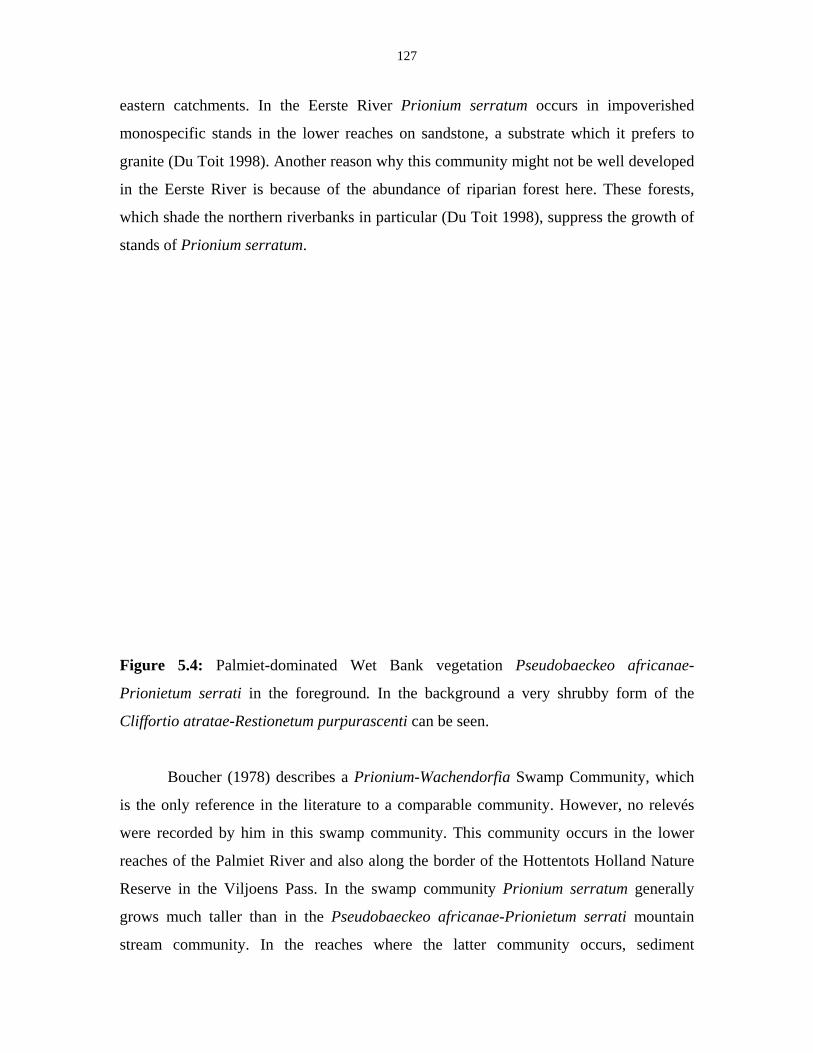
127
eastern catchments. In the Eerste River Prionium serratum occurs in impoverished
monospecific stands in the lower reaches on sandstone, a substrate which it prefers to
granite (Du Toit 1998). Another reason why this community might not be well developed
in the Eerste River is because of the abundance of riparian forest here. These forests,
which shade the northern riverbanks in particular (Du Toit 1998), suppress the growth of
stands of Prionium serratum.
Figure 5.4: Palmiet-dominated Wet Bank vegetation Pseudobaeckeo africanae-
Prionietum serrati in the foreground. In the background a very shrubby form of the
Cliffortio atratae-Restionetum purpurascenti can be seen.
Boucher (1978) describes a Prionium-Wachendorfia Swamp Community, which
is the only reference in the literature to a comparable community. However, no relevés
were recorded by him in this swamp community. This community occurs in the lower
reaches of the Palmiet River and also along the border of the Hottentots Holland Nature
Reserve in the Viljoens Pass. In the swamp community Prionium serratum generally
grows much taller than in the Pseudobaeckeo africanae-Prionietum serrati mountain
stream community. In the reaches where the latter community occurs, sediment
128
deposition takes place rather than erosion. This makes it a completely different ecological
system. Taylor (1978) categorizes both types of Prionium communities as Hygrophilous
Fynbos, but this is not a consistent floristic unit.
Community Group 4: Deposition Wetbanks
This Community Group contains only one community in the area. It is found in the lower
reaches where sediment loads are deposited in the Foothill Zone. It is very exposed and
the vegetation is sparse. It can occur in both the Upper and the Lower Wet Bank Zones.
Community type 4.1: Wimmerella bifida-Juncus lomatophyllus Open Sedgeland
Scientific name: Wimmerello bifidae-Juncetum lomatophylli ass. nova hoc loco
Number of relevés: 6
Type relevé: 146 (Table 3)
Average no. of species: 18 (9 – 30)
This community is found on open beaches where sand accumulates in the reaches where
the river enters the Foothill Zone. The vegetation mainly consists of sedges, with some
Restionaceae and grasses. The soils are sandy and contain many cobbles. Most samples
of this type have been found where the Riviersonderend River leaves the mountains and
enters the plains near Theewaterskloof Dam. Here the community is very well developed.
An additional sample from the Lourens River shows that this community can also occur
in higher reaches, but in a depauperate form.
The community occurs in its optimal form on open sandy beaches. Here a slight
zonation pattern occurs, but it is not distinct enough to be illustrated by the data available
in this study. Further research might show that this association contains a number of
subassociations. Because the banks formed by sandy beaches are often very flat, very
small fluctuations in water level reflect marked differences in the horizontal distribution
of species. Isolepis prolifer grows closest to the water where it binds the accumulating
sand so that Juncus lomatophyllus can then colonize the sand at elevations of just a few
centimetres higher than the Isolepis prolifer Zone. Juncus lomatophyllus forms the
129
dominant species in this vegetation type. Higher up the bank Calopsis paniculata,
Pennisetum macrourum and Pentameris thuarii can be found. These species, together
with several juveniles of shrubs such as Brachylaena neriifolia and Morella serrata, form
a vegetation belt that holds the sand firmly. Two other differential species found in this
zone and the next one are Wimmerella bifida and Juncus capensis.
If the beach is wide enough there is also a zone higher up the beach where the
sand is very dry and subject to wind erosion. Barely any plants grow here, because of the
unstable environment. This shows clearly that the structure of this vegetation type is
highly variable. In the Isolepis prolifer Zone the vegetation is low and dense; in the
Pennisetum macrourum Zone the vegetation is tall and dense and higher up the beach the
vegetation is low and sparse.
Ericaceous and Transitional Fynbos communities (Appendix E; Table 4)
The communities in Table 4 are found in the Lower and Upper Dynamic Zones of the
rivers and consist of two Community Groups. Community Group 5 consists of
communities that fit Campbell’s (1986b) description of Ericaceous Fynbos. However,
this author might have classified some of the relevés as Proteoid Fynbos when the
proteoid Leucadendron xanthoconus has a high cover in the relevé. This example shows
that structurally different types can be closely related floristically in the Fynbos Biome.
This was also concluded by Werger et al. (1972) in Waboomveld (Protea nitida
vegetation). The structural classification of Campbell (1986b) does not provide much
information in these situations. Community Group 6 consists of some unrelated
communities that are somehow transitional between Community Group 5 and
Community Group 7 (shown in Appendix C; Table 5).
Community Group 5: Ericaceous Fynbos
The following group of communities is very diverse and contains the most species-rich
vegetation samples found in this study. Vegetation can be below half a meter tall and
only consist of dwarf shrubs, or it can be taller than three metres. The total vegetation
130
cover is always more than 70 %. One species that all these communities have in common
is Erica hispidula; however, this species also occurs in the Asteraceous Fynbos and in the
Upper Wet Bank Zones. The following differential species are shared with the
Pseudobaeckeo africanae-Prionietum serrati described above, namely: Penaea cneorum,
Erica lutea, Berzelia squarrosa and Restio purpurascens. There are three differential
species that are not shared with any other Community Group, namely: Erica
equisetifolia, Erica longifolia and Capeobolus brevicaulis. The shrubs Leucadendron
xanthoconus and Brunia alopecuroides are only shared with Community Group 6.
Related communities in the literature are the Erica viridescens-Hypodiscus
aristatus Community (Bond 1981), the Tetraria thermalis-Hypodiscus aristatus
Community (Kruger 1974), bergpalmietveld (Taylor 1978), the Leptocarpus
membranaceus-Hypodiscus aristatus Community (McKenzie et al. 1977) and the
Penaea-Erica Fynbos Community subcommunities B and C (Glyphis et al. 1978). The
species that are in common between these communities are: Aristea major, Capeobolus
brevicaulis, Chrysithrix capensis, Cliffortia atrata, Erica hispidula, E. plukenetii,
Helichrysum felinum, Hypodiscus aristatus, Leucadendron xanthoconus, Penaea
cneorum, Restio bifarius, Tetraria cuspidata, T. thermalis and Widdringtonia nodiflora.
Campbell (1986b) classifies all these types as belonging to his Nuweberg Mesic
Ericaceous Fynbos. The communities described below all occur on shallow acid soils that
consist mainly of medium textured sands derived from Table Mountain Group
sandstones.
131
Community type 5.1: Ischyrolepis triflora-Protea grandiceps Closed Tall Shrubland
Number of relevés: 2
Range of species number: 45 – 46
A very distinct vegetation type, which is only represented here by two relevés, occurs in
the highest reaches of the Lourens River catchment. It occurs on sandstone and can be
described as a seepage area on a steep slope dominated by Berzelia squarrosa. Soils are
relatively deep and acidic and the drainage is quite good. There is a high cover of rocks,
which line the gullies draining the slopes. The western slopes of Somerset Sneeukop that
are drained by the Lourens River belong to the steepest altitudinal and climatic gradients
found in the region and mist is probably quite common. The vegetation occurs in two
strata: a herb stratum, which is the dominant stratum and a low shrub stratum 1.5 – 2.0 m
tall, which covers 20% of the relevé. This is one of the most species-rich vegetation types
found in riparian habitats in the area. It contains many species that are absent or rare in
the other types, such as Cliffortia integerrima, Galium tomentosum, Protea grandiceps,
Psoralea asarina, Struthiola martiana and Willdenowia sulcata.
Community type 5.2: Nebelia fragarioides-Staberoha cernua Closed Short Shrubland
Number of relevés: 4
Average no. of species: 19 (8 – 28)
This is a very low vegetation type (generally below 0.5 m) on sandstone that occurs in
the extreme south of the study area in the Palmiet River catchment. It is dominated by
Brunia alopecuroides and Erica intervallaris. Structurally, it resembles a transition
between a restio marsh and a riverbank, because the vegetation is very low (mostly lower
than 0.5 m). It is a vegetation type that contains many southern elements and similar
communities were found in the Kogelberg Biosphere Reserve (Boucher 1978; compare
Table 5.8). These communities probably belong to the same alliance. Differential species
that are typical are Chironia jasminoides, Nebelia fragarioides, Nevillea obtusissima,
Staberoha cernua and Tetraria capillacea.
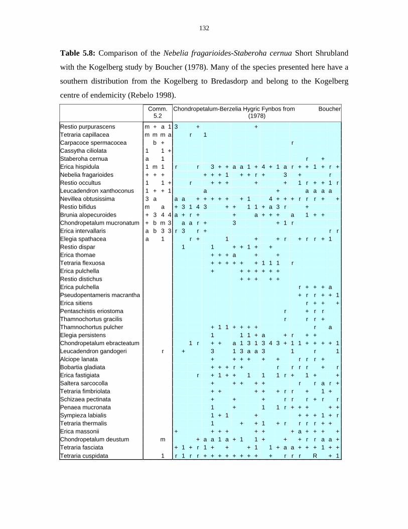
132
Table 5.8: Comparison of the Nebelia fragarioides-Staberoha cernua Short Shrubland
with the Kogelberg study by Boucher (1978). Many of the species presented here have a
southern distribution from the Kogelberg to Bredasdorp and belong to the Kogelberg
centre of endemicity (Rebelo 1998).
Comm. 5.2
Chondropetalum-Berzelia Hygric Fynbos from Boucher (1978)
Restio purpurascens m + a 1 3 + + Tetraria capillacea m m m a r 1 Carpacoce spermacocea b + r Cassytha ciliolata 1 1 + Staberoha cernua a 1 r + Erica hispidula 1 m 1 r r 3 + + a a 1 + 4 + 1 a r + + 1 + r +Nebelia fragarioides + + + + + + 1 + + r + 3 + r Restio occultus 1 1 + r + + + + + 1 r + + 1 rLeucadendron xanthoconus 1 + + 1 a + a a a a Nevillea obtusissima 3 a a a + + + + + + 1 4 + + + r r r + +Restio bifidus m a + 3 1 4 3 + + 1 1 + a 3 r + Brunia alopecuroides + 3 4 4 a + r + + a + + + a 1 + + Chondropetalum mucronatum + b m 3 a a r + 3 + 1 r Erica intervallaris a b 3 3 r 3 r + r rElegia spathacea a 1 r + 1 + + r + r r + 1 Restio dispar 1 1 + + 1 + + Erica thomae + + + a + + Tetraria flexuosa + + + + + + 1 1 1 r Erica pulchella + + + + + + + Restio distichus + + + + + Erica pulchella r + + + a Pseudopentameris macrantha + r r + + 1Erica sitiens r + + +Pentaschistis eriostoma r + r r Thamnochortus gracilis r r r + Thamnochortus pulcher + 1 1 + + + + r a Elegia persistens 1 1 1 + a + r + + Chondropetalum ebracteatum 1 r + + a 1 3 1 3 4 3 + 1 1 + + + + 1Leucadendron gandogeri r + 3 1 3 a a 3 1 r 1Alciope lanata + + + + + + r r r + Bobartia gladiata + + + r + r r r r + rErica fastigiata r + 1 + + 1 1 1 r + 1 + +Saltera sarcocolla + + + + + r r a r +Tetraria fimbriolata + + + + + r r + 1 + Schizaea pectinata + + + r r r + r rPenaea mucronata 1 + 1 1 r + + + + +Sympieza labialis 1 + 1 + + + + 1 + rTetraria thermalis 1 + + 1 + r r r r + + Erica massonii + + + + + + + a + + + +Chondropetalum deustum m + a a 1 a + 1 1 + + + r r a a +Tetraria fasciata + 1 + r 1 + + + 1 1 + a a + + + 1 + +Tetraria cuspidata 1 r 1 r r + + + + + + + + + r r r R + 1
133
The soil is quite acidic here with pH lower than 4 and the substrate is less rocky
than the other Ericaceous Fynbos types. The organic matter contents are low close to the
river but higher in the Back Dynamic Zone.
Community type 5.3: Erica longifolia-Tetraria crassa Closed Short Shrubland.
Scientific name: Erico longifoliae-Tetrarietum crassae ass. nova hoc loco
Number of relevés: 7
Type relevé: 216 (Table 4)
Average no. of species: 41 (27 – 55)
This is one of the most species-rich riparian communities found in this study. It
sometimes supports more than 70 species on a surface area of 30 m2. It is found at higher
altitudes in the Palmiet and Riviersonderend River catchments. One relevé (no. 263) was
collected outside the actual study area in the Groenland Mountains. The community
occurs in places that receive more rainfall than any of the other Ericaceous Fynbos types
and mist is quite common. The community occurs on shallow soils of the Mispah Form
with many boulders. It contains typical seepage species (see Chapter 4), like Restio
subtilis and R. aff. versatilis, which indicates that this community grows in a wet habitat.
Half of the relevés have a shrub layer, 2.0 – 3.0 m tall, covering 20% of the relevé
and consisting of species such as Brachylaena neriifolia and Podalyria aff. montana. The
herb layer, which is dominant, is relatively low (mostly shorter than 0.5 m).
Especially Ericaceae (Erica fastigiata, E. longifolia, E. lutea, E. plukenetii and E.
sessiliflora) and Restionaceae (Chondropetalum deustum, Elegia neesii, E. spathacea
Restio bifidus, R. burchelli, R. corneolus, R. subtilis, R. aff. versatilis and Staberoha
vaginata) have a large number of species and a high cover in these communities. Less
conspicuous, but also important constituents of this vegetation type are the sedges,
especially Tetraria spp. (T. bromoides, T. crassa, and T. pillansii).
134
Community type 5.4: Cliffortia atrata-Restio purpurascens Closed Tall Shrubland
Scientific name: Cliffortio atratae-Restionetum purpurascentis ass. nova hoc loco
Number of relevés: 20
Type relevé: 225 (Table 4)
Average no. of species: 25 (11 – 38)
This is the most common of the Ericaceous Fynbos types. It is subdivided into two
subassociations, of which one occurs in mesic habitats and the other in xeric habitats.
They are found in the eastern half of the mountains on sandstone in the Back Dynamic
Zones of the rivers. The vegetation consists of a shrub layer 2.0 – 4.0 m tall, covering
20% or more of the community and a dominant herb layer 0.5 – 1.0 m tall. The tallest
constituents of the herb layer are the Restionaceae, especially the common species Restio
purpurascens. This vegetation type is quite similar to the surrounding fynbos in the
uplands, except for the presence of Restio purpurascens and occasional plants of
Brachylaena neriifolia, Penaea cneorum, and a number of Bruniaceae species, that grow
in the wetter conditions near the river. Higher up the slope, Tetraria thermalis usually
becomes more dominant and occurs in patches. This is the vegetation type that Taylor
(1978) refers to as ‘bergpalmietveld’, referring to the common name for Tetraria
thermalis. The community has few differential species at the association level
(Askidiosperma esterhuyseniae, Chrysithrix capensis, Cliffortia atrata and Coleonema
juniperum). Most of the differential species will be discussed at the subassociation level.
Subassociation 5.4a: Cliffortio atratae-Restionetum purpurascentis typicum subass. nova
hoc loco
Number of relevés: 12
Type relevé: 225 (Table 3)
Average no. of species: 23 (13 – 30)
This is the nutrient-poor form of the community that occurs on the drier mineral soils
with a higher pH. The soils are also rockier than in the mesic subassociation. Differential
species are Ceratocaryum argenteum, Pentameris macrocalycina and Pseudobaeckea
africana. Some additional differential species at the subassociation level are shared with
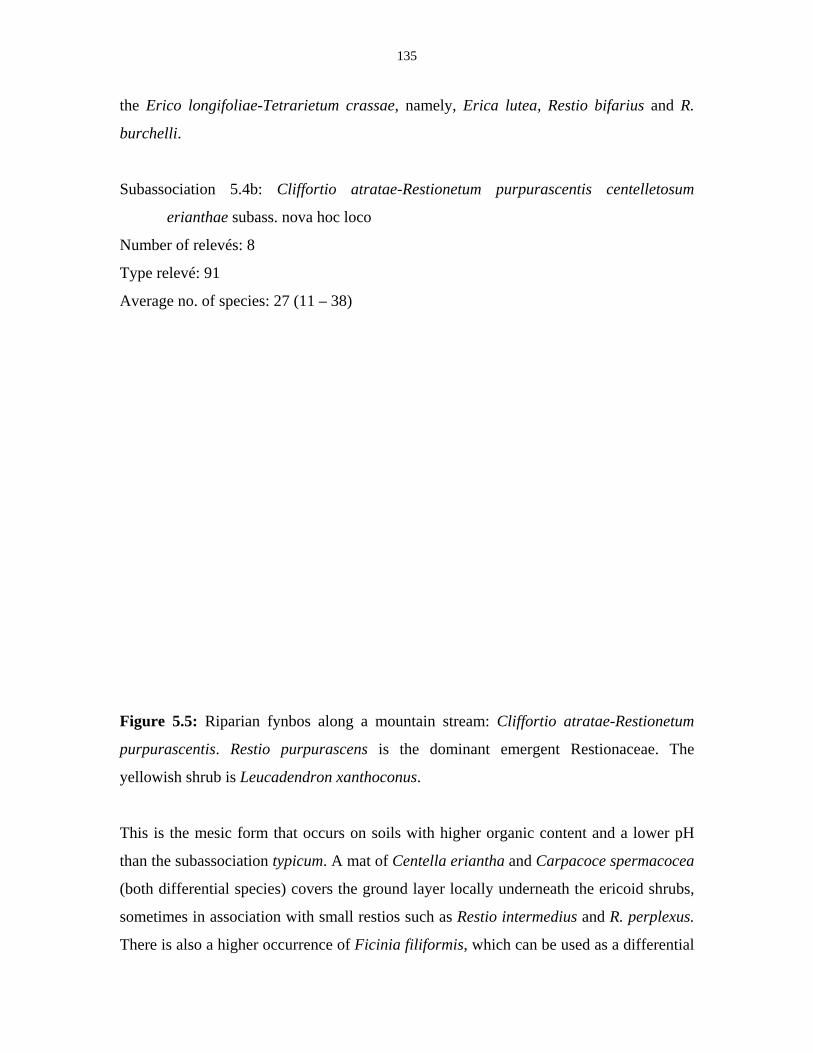
135
the Erico longifoliae-Tetrarietum crassae, namely, Erica lutea, Restio bifarius and R.
burchelli.
Subassociation 5.4b: Cliffortio atratae-Restionetum purpurascentis centelletosum
erianthae subass. nova hoc loco
Number of relevés: 8
Type relevé: 91
Average no. of species: 27 (11 – 38)
Figure 5.5: Riparian fynbos along a mountain stream: Cliffortio atratae-Restionetum
purpurascentis. Restio purpurascens is the dominant emergent Restionaceae. The
yellowish shrub is Leucadendron xanthoconus.
This is the mesic form that occurs on soils with higher organic content and a lower pH
than the subassociation typicum. A mat of Centella eriantha and Carpacoce spermacocea
(both differential species) covers the ground layer locally underneath the ericoid shrubs,
sometimes in association with small restios such as Restio intermedius and R. perplexus.
There is also a higher occurrence of Ficinia filiformis, which can be used as a differential
136
species of this subassociation. The vegetation is dominated by Restio purpurascens and
Erica hispidula.
Community type 5.5: Restio purpurascens-Cliffortia hirsuta Closed Tall Shrubland
Scientific name: Restio purpurascenti-Cliffortietum hirsutae ass. nova hoc loco
Number of relevés: 4
Type relevé: 223 (Table 4)
Average no. of species: 26 (22 – 37)
This is a very shrubby community, which is related to the Elegia capensis-Cliffortia
hirsuta Closed Tall Shrubland of Community Group 6 (see below; Community 6.1). It
occurs in places where there is seepage from the slopes into the river. Because of the wet
conditions, some typical Wet Bank species such as Drosera capensis or Schizaea tenella
can occur in the lower strata. A shrub stratum, 1.5 – 2.5 m tall, is present in all but one of
the relevés and generally covers more than 50% of the sample plot. The herb layer
consists of two different height classes, the tallest (1.0 – 1.5 m), formed by Cliffortia
hirsuta, being dominant. The low herbs are about 0.5 m tall. Differential species are
Cliffortia hirsuta and possibly also Erica curviflora, Elegia thyrsifera and Neesenbeckia
punctoria, which are shared with Cliffortio atratae-Restionetum purpurascentis.
Some samples have been taken on a shale substrate, but the pH is relatively low
(around pH 4), probably because of mixing with sandstone rubble originating from the
immediate environment. The lowest parts of the Palmiet River and a significant part of
Noordekloof belong to this vegetation type. Additional data from this community would
be useful although it is quite characteristic, hence a formal scientific name was given to it
here.
Boucher (1978) mentions the occurrence of Cliffortia hirsuta and Neesenbeckia
punctoria together in his Erica-Osmitopsis Seepage Fynbos. Floristically and
ecologically these communities have the seepage aspect in common, although they are
clearly different communities.
137
Community Group 6: Transitional Fynbos
These are three different communities that are transitional between the Ericaceous
Fynbos of Community Group 5 and the Asteraceous Fynbos of Community Group 7.
They do not seem to be closely related amongst each other however, so they are treated
separately.
Community type 6.1: Elegia capensis-Cliffortia hirsuta Closed Tall Shrubland
Number of relevés: 2
Range of species number: 10 – 19
This community seems to be an extreme form of the Restio purpurascenti-Cliffortietum
hirsutae, in which Cliffortia hirsuta dominates and the typical species of the Ericaceous
Fynbos communities, such as Erica hispidula, Leucadendron xanthoconus and Restio
purpurascens are absent. Only two transects having this community were sampled: one in
Boesmanskloof, where it seems to be quite extensive, and one in Wolwekloof. It is a very
species-poor community completely dominated by dense stands of Cliffortia hirsuta. The
other species that are differential for this community are Elegia capensis, Ficinia
trichodes and the peculiar species Psoralea fleta. This is a very tall and slender shrub (up
to 5.0 metres tall) that offers a very sparse overstorey. The understorey of Cliffortia
hirsuta and Elegia capensis is mostly about 1.5 – 2.0 m tall and covers the entire relevé.
The community occurs on dark sandy soils with a pH of 4.

138
Community type 6.2: Muraltia heisteria-Erica pinea Closed Tall Shrubland
Scientific name: Muraltio heisteriae-Ericetum pineae ass. nova hoc loco
Number of relevés: 7
Type relevé: 248 (Table 4)
Average no. of species: 28 (19 – 39).
This community is transitional between the Ericaceous Fynbos communities and the
Riparian Scrub communities. It is structurally similar to the Helichryso-Myrsinietum
africanae of Community Group 7 and to the Brabejum stellatifolium Community of
Werger et al. (1972), but it contains many elements of the Ericaceous Fynbos group.
Campbell (1986b) would classify this community as Witrivier Closed-Scrub Fynbos
together with the scrubland communities of the Ischyrolepido-Metrosiderotetum
angustifoliae (see Appendix E; Table 6), but the main difference from the other Closed-
Scrub Fynbos types is the extensive cover of the herb layer (more than 70% cover),
which is very weakly developed in the Ischyrolepido-Metrosiderotetum angustifoliae.
Taylor (1978) would call this community type, and the other Closed-Scrub Fynbos
communities, Hygrophilous Fynbos. Except for the herb layer, there is a shrub layer
present in which Brabejum stellatifolium (differential), Leucadendron xanthoconus
(dominant), Metrosideros angustifolia and Podalyria calyptrata are the most important
species. Some of the lower shrubs that are present are Diospyros glabra, Muraltia
heisteria, Cliffortia grandifolia and Liparia capitata. The last two are differential
species, together with the herbs Erica nudiflora, E. pinea and Elegia asperiflora. The
exotic shrub, Hakea sericea, is often present. The shrub layer covers about 30% of a
relevé and ranges in height between 1.5 and 3.0 metres. The herb layer also contains
some tall species, especially Restionaceae, like Cannomois virgata, Restio dispar and
Platycaulos callistachyus, which grow to 1.5 m tall. The most common species in the
herb layer is Pteridium aquilinum.
In the Hottentots Holland Mountains this community is only found in the extreme
north, at Jan Joubertsgat. The Mean Annual Precipitation is low (less than 1000 mm) and
the difference in rainfall between January and July is high, with July having more than
ten times the amount falling in January. This means that there is likely to be water-stress
139
in summer, although the riparian communities will not suffer too much from that. The
community occurs on relatively deep mineral soils with a relatively high pH between 4.5
and 5.0. The boundary between this community and the stony Wet Bank is very sharp.
There seems to be a subdivision between samples with and without Brabejum
stellatifolium and Erica pinea. Not much attention has been paid to this possible
distinction because the relevés were all taken from the same locality and the number of
relevés is not very high.
Community type 6.3: Euryops abrotanifolius-Haplocarpha lanata Closed Tall Shrubland
Number of relevés: 2
Range of species number: 29 – 39
This community represents the vegetation of the Back Dynamic Zone in
Assegaaiboschkloof. It is a mixture of riverine elements and the vegetation from the
slopes of Assegaaiboschkloof, which is a form of Talus Asteraceous Fynbos (Campbell
1986b). Because the Riverine Shrub Zone is often very wide in this area and there is a lot
of riparian forest, this fynbos vegetation rarely penetrates into the riparian zone. This
explains why only two relevés were recorded in this type. The vegetation is mostly
herbaceous with only a very sparse shrub layer (10% cover, consisting of species such as
Cassine schinoides and Metrosideros angustifolia). Some of the differential species in
this herbaceous layer are Cliffortia ruscifolia, Gibbaria ilicifolia, Haplocarpha lanata,
Helichrysum cymosum and Othonna quinquedentata. The soils are shallow and very
stony for a Back Dynamic Zone. They are slightly acidic (pH 4.5).
Asteraceous Fynbos and Renosterveld communities (Appendix E; Table 5)
The communities in this table are taken from the Back Dynamic Zones of the western and
northern slopes of the Hottentots Holland Mountains, mainly in the Berg and Eerste
River Catchments. There are relevés located on shale, granite and sandstone substrates,
but only the communities on shale stand out as separate entities. These are sampled in the
Moordenaarskloof of the Stellenbosch Mountains, where shales from the Malmesbury
140
Group are exposed (See Fig. 2.6 and South African Committee for Stratigraphy 1980).
One of these is related to the Asteraceous Fynbos communities found on granite or
sandstone in Jonkershoek and the other is completely different, namely a monospecific
community of Cliffortia odorata. The communities dominated by this species are
clustered in Community Group 8.
Community Group 7: Asteraceous Fynbos
This Community group consists of Asteraceous Fynbos, in which the ‘typical’ fynbos
elements like ericas, restios and proteas are less pronounced (The only differential Erica-
species is Erica hirta. However it contains many species of Asteraceae, ferns and sedges
(especially Ficinia spp.; Ficinia trichodes is a differential species). It also has a more
distinct shrubby element and grows taller than most Ericaceous Fynbos types. Some other
differential species are Cliffortia cuneata, Myrsine africana and Oxalis livida.
The communities in this group occur on the yellow plinthic soils found on
granites or shale, which occur mostly on the western side of the mountain range. In
Assegaaibosch Kloof they are also found on sandstone. Campbell (1986b) did not
mention these vegetation types, which are typically riparian, but the Talus Asteraceous
Fynbos or Waboomveld is very similar to it.
This community group shares many species with forest and scrub, namely:
Asparagus scandens, Blechnum punctulatum, Halleria elliptica, Ischyrolepis
gaudichaudiana, Myrsine africana and Pteridium aquilinum. The only tree that typically
occurs outside of the forest, Maytenus oleoides, is regularly found in these communities.
Another tree species, Cassine schinoides, is in these communities restricted to the lower
shrub stratum and does not grow any taller.
141
Community type 7.1: Wahlenbergia parvifolia-Pentameris thuarii Closed Tall Grassland
Scientific name: Wahlenbergio parvifoliae-Pentameritetum thuarii ass. nova hoc loco
Number of relevés: 5
Type relevé: 196 (Table 5)
Average no. of species: 28 (20 – 38)
This community would not have been recognized as fynbos by Campbell (1986b)
because of the high cover of grasses and it is best described as a Tall Grassland (Edwards
1983). However, from a floristical point of view, it is closely related to the Helichryso
cymosi-Myrsinietum africanae that is clearly fynbos. The marked dominance of the grass
Pentameris thuarii makes this community distinct, even from a considerable distance, as
it appears as yellowish patches in the seepage zones around riparian forests in
Swartboschkloof and Diepgat Ravine. It is also found in the riverbeds of seasonal rivers.
In many instances it can extend for a long distance away from the rivers themselves. The
vegetation consists of two herb layers, the tallest of which is dominated by the tall
graminoids Pentameris thuarii and Pennisetum macrourum (both differential species).
This layer is 1.0 – 1.5 m tall and covers the entire plot. Some shrubs and tall herbs also
grow in this layer but rarely become emergent to form an own shrub layer, such as
Othonna quinquedentata, Psoralea pinnata and Rhus angustifolia. The lower herb layer
is about 0.5 m tall and is found sparsely distributed between the grass. The most
important species in this layer are: Pteridium aquilinum (dominant), Cullumia setosa,
Helichrysum helianthemifolium, H. foetidum, Phylica pubescens (juv.), Pseudoselago
serrata and Wahlenbergia parvifolia. The last four species are also differential.
It is peculiar that this community was not recorded by McDonald (1988) in his
vegetation survey of Swartboschkloof in 1983. It is also not visible on a clear picture of
the valley from 1973 shown in Van Wilgen & McDonald (1992). Because the last fire in
Swartboschkloof prior to 1973 was in 1958 (Van Wilgen & McDonald 1992; McDonald
1988) it seems likely that this vegetation type will be replaced by another later in the
successional stage. Pentameris thuarii is a pioneer species after fire and it was found
throughout the area after the fire of April 1999. It is interesting to note that in some
places the species manages to persist for a much longer time and grows into a tough
142
woody grass. In Swartboschkloof it has persisted for 12 years since the fire in 1987. The
differences might be caused by a different fire intensity or fire season. A better
understanding of this vegetation type can be obtained by studying the autecology and fire
response of this species. The soils on which this tall grassland type occurs are shallow
mineral soils on granite with a pH of around 4.5.
Community type 7.2: Helichrysum cymosum-Myrsine africana Closed Short to Tall
Shrubland
Scientific name: Helichryso cymosi-Myrsinietum africanae ass. nova hoc loco
Number of relevés: 18
Type relevé: 175 (Table 5)
Average no. of species: 25 (14 – 42)
This association is quite variable and there are two subassociations described together
with one undersampled subcommunity. The two subassociations differ mainly in their
structure, one is low and fynbos-like and the other is in succession to a scrub-community,
and is poorer in species. The undersampled subcommunity is also poor in species and is
found in the higher reaches of the Eerste River. The most important differential species
are Agathosma crenulata, Metalasia cephalotes and Stoebe cinerea. Within Community
Group 7, Erica hispidula is also differential for this community. Both subassociations
occur typically in the Back Dynamic Zone on sandstone or granite. It is found in
Jonkershoek and the lower reaches of the Berg River catchment. Campbell (1986b)
would describe it as a riverine form of Talus Asteraceous Fynbos. Werger et al. (1972),
described it as Brabejum stellatifolium Community, which suggests that they only found
the subassociation inops. McDonald (1988) mentions this type as Halleria elliptica-
Cliffortia cuneata High Closed Shrubland, which is a good description for the
subassociation ficinietosum acuminati described here.
The comparison with the McDonald (1988) and Werger et al. (1972) studies is
shown in Table 5.9. This table shows that there is actually a gradient from Waboomveld
to Brabejum Scrub and the Helichryso-Myrsinietum africanae is situated between them.
The Brabejum Scrub was not clearly identified in this study. It is most common on talus
143
slopes in Swartboschkloof. The soils are brown or yellowish and shallow, while the pH is
around 4.5. McDonald (1988) mentions the following soils occurring in association with
this community: Hutton, Fernwood, Magwa and Oakleaf Forms (see also Fry 1987).
The new classification of the data that can be seen in Table 5.9 results in some
shifts of relevés from one cluster to another; that is why the names of the vegetation types
are only stated in general terms. The exact classification of all data will become clear
during the VEGMAP project (McDonald 1997; McDonald & Boucher 1999).
Subassociation 7.2a: Helichryso cymosi-Myrsinietum africanae ficinietosum acuminatae
subass. nova hoc loco
Number of relevés: 9
Type relevé: 175 (Table 5)
Average no. of species: 26 (14 – 42)
This is the structurally shorter herbaceous form of the association, which is richer in
species than the taller shrubby form, because there is more diversity in the niches within
it. Shrubs do occur but cover on average only 20% of each relevé. Herbs shape the
dominant stratum and the most common species, Ischyrolepis subverticillata, is a 1.5 m
tall Restionaceae. Differential species are the shrub Otholobium obliquum, the two
inconspicuous sedges Ficinia acuminata and F. nigrescens and the vine Dipogon
lignosus.
Subassociation 7.2b: Helichryso cymosi-Myrsinietum africanae inops subass. nova hoc
loco
Number of relevés: 7
Type relevé: 180 (Table 5)
Average no. of species: 25 (19 – 29) Table 5.9: Comparison between the Communities 7.1, 7.2a, 7.2b and 7.3c (respectively in columns 4, 5, 6 and 7) with two other studies in Jonkershoek (Werger et al. 1972 and McDonald 1988). A gradient from Waboomveld to Riparian Scrub is clearly illustrated in this table. The first three columns represent several types of Waboomveld or Talus Asteraceous Fynbos (including relevé 99 from the present study in column
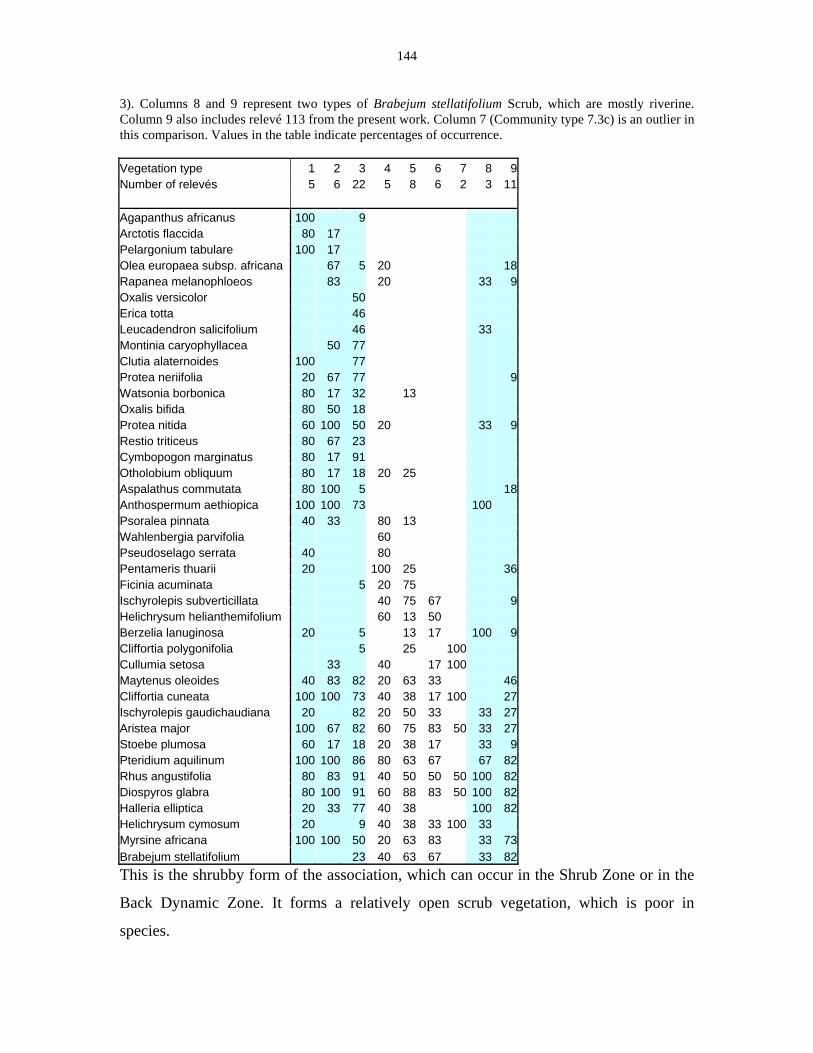
144
3). Columns 8 and 9 represent two types of Brabejum stellatifolium Scrub, which are mostly riverine. Column 9 also includes relevé 113 from the present work. Column 7 (Community type 7.3c) is an outlier in this comparison. Values in the table indicate percentages of occurrence. Vegetation type 1 2 3 4 5 6 7 8 9Number of relevés 5 6 22 5 8 6 2 3 11 Agapanthus africanus 100 9 Arctotis flaccida 80 17 Pelargonium tabulare 100 17 Olea europaea subsp. africana 67 5 20 18Rapanea melanophloeos 83 20 33 9Oxalis versicolor 50 Erica totta 46 Leucadendron salicifolium 46 33 Montinia caryophyllacea 50 77 Clutia alaternoides 100 77 Protea neriifolia 20 67 77 9Watsonia borbonica 80 17 32 13 Oxalis bifida 80 50 18 Protea nitida 60 100 50 20 33 9Restio triticeus 80 67 23 Cymbopogon marginatus 80 17 91 Otholobium obliquum 80 17 18 20 25 Aspalathus commutata 80 100 5 18Anthospermum aethiopica 100 100 73 100 Psoralea pinnata 40 33 80 13 Wahlenbergia parvifolia 60 Pseudoselago serrata 40 80 Pentameris thuarii 20 100 25 36Ficinia acuminata 5 20 75 Ischyrolepis subverticillata 40 75 67 9Helichrysum helianthemifolium 60 13 50 Berzelia lanuginosa 20 5 13 17 100 9Cliffortia polygonifolia 5 25 100 Cullumia setosa 33 40 17 100 Maytenus oleoides 40 83 82 20 63 33 46Cliffortia cuneata 100 100 73 40 38 17 100 27Ischyrolepis gaudichaudiana 20 82 20 50 33 33 27Aristea major 100 67 82 60 75 83 50 33 27Stoebe plumosa 60 17 18 20 38 17 33 9Pteridium aquilinum 100 100 86 80 63 67 67 82Rhus angustifolia 80 83 91 40 50 50 50 100 82Diospyros glabra 80 100 91 60 88 83 50 100 82Halleria elliptica 20 33 77 40 38 100 82Helichrysum cymosum 20 9 40 38 33 100 33 Myrsine africana 100 100 50 20 63 83 33 73Brabejum stellatifolium 23 40 63 67 33 82This is the shrubby form of the association, which can occur in the Shrub Zone or in the
Back Dynamic Zone. It forms a relatively open scrub vegetation, which is poor in
species.
145
In two of the relevés there is a tree stratum 4.0 – 6.0 m tall, which covers more
than 70% of the plot. A shrub stratum of 2.0 – 4.0 m is more common and covers about
40% of the relevé. The dominant shrub is Brabejum stellatifolium, but Cassine schinoides
is also common. The herb layer is in most cases sparse; it only covers about 50% or less
of each relevé.
Subcommunity 7.2c: Cliffortia polygonifolia-Cullumia setosa Variant
Number of relevés: 2
Range of species number: 20 – 25
This subcommunity was sampled twice at high altitude in Jonkershoek in a river reach
where the Back Dynamic Zone was not well developed. It is best characterized by the
absence of some typical Helichryso-Myrsinietum africanae species such as Halleria
elliptica and Myrsine africana. The vegetation here is very dense with a shrub layer that
covers about 60% and a herb layer that covers nearly the whole plot. The Shrub layer is
dominated by Podalyria calyptrata and Cliffortia cuneata, while some of the typical
species in the herb layer are Cullumia setosa, Cliffortia polygonifolia and Pelargonium
hermanniifolium. This community occurs in similar environmental conditions as the other
Helichryso-Myrsinietum africanae communities, but at a higher altitude. Also, one of the
two samples occurs on a soil that is richer in organic material than in the other
Helichryso-Myrsinietum africanae subcommunities.
Community type 7.3: Pelargonium tomentosum-Chasmanthe aethiopica Closed Tall
Shrubland
Scientific name: Pelargonio tomentosi-Chasmanthetum aethiopicae ass. nova hoc loco
Number of relevés: 5.
Type relevé: 67 (Table 5)
Average no. of species: 33 (24 – 40)
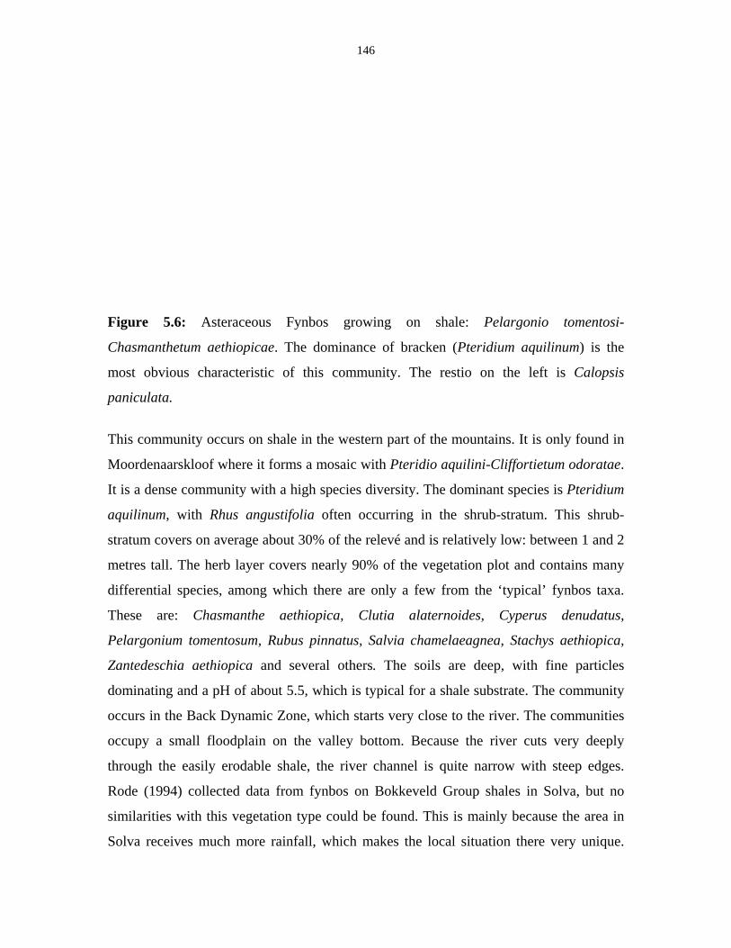
146
Figure 5.6: Asteraceous Fynbos growing on shale: Pelargonio tomentosi-
Chasmanthetum aethiopicae. The dominance of bracken (Pteridium aquilinum) is the
most obvious characteristic of this community. The restio on the left is Calopsis
paniculata.
This community occurs on shale in the western part of the mountains. It is only found in
Moordenaarskloof where it forms a mosaic with Pteridio aquilini-Cliffortietum odoratae.
It is a dense community with a high species diversity. The dominant species is Pteridium
aquilinum, with Rhus angustifolia often occurring in the shrub-stratum. This shrub-
stratum covers on average about 30% of the relevé and is relatively low: between 1 and 2
metres tall. The herb layer covers nearly 90% of the vegetation plot and contains many
differential species, among which there are only a few from the ‘typical’ fynbos taxa.
These are: Chasmanthe aethiopica, Clutia alaternoides, Cyperus denudatus,
Pelargonium tomentosum, Rubus pinnatus, Salvia chamelaeagnea, Stachys aethiopica,
Zantedeschia aethiopica and several others. The soils are deep, with fine particles
dominating and a pH of about 5.5, which is typical for a shale substrate. The community
occurs in the Back Dynamic Zone, which starts very close to the river. The communities
occupy a small floodplain on the valley bottom. Because the river cuts very deeply
through the easily erodable shale, the river channel is quite narrow with steep edges.
Rode (1994) collected data from fynbos on Bokkeveld Group shales in Solva, but no
similarities with this vegetation type could be found. This is mainly because the area in
Solva receives much more rainfall, which makes the local situation there very unique.
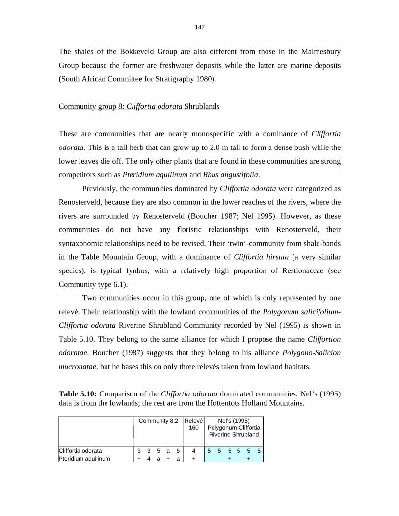
147
The shales of the Bokkeveld Group are also different from those in the Malmesbury
Group because the former are freshwater deposits while the latter are marine deposits
(South African Committee for Stratigraphy 1980).
Community group 8: Cliffortia odorata Shrublands
These are communities that are nearly monospecific with a dominance of Cliffortia
odorata. This is a tall herb that can grow up to 2.0 m tall to form a dense bush while the
lower leaves die off. The only other plants that are found in these communities are strong
competitors such as Pteridium aquilinum and Rhus angustifolia.
Previously, the communities dominated by Cliffortia odorata were categorized as
Renosterveld, because they are also common in the lower reaches of the rivers, where the
rivers are surrounded by Renosterveld (Boucher 1987; Nel 1995). However, as these
communities do not have any floristic relationships with Renosterveld, their
syntaxonomic relationships need to be revised. Their ‘twin’-community from shale-bands
in the Table Mountain Group, with a dominance of Cliffortia hirsuta (a very similar
species), is typical fynbos, with a relatively high proportion of Restionaceae (see
Community type 6.1).
Two communities occur in this group, one of which is only represented by one
relevé. Their relationship with the lowland communities of the Polygonum salicifolium-
Cliffortia odorata Riverine Shrubland Community recorded by Nel (1995) is shown in
Table 5.10. They belong to the same alliance for which I propose the name Cliffortion
odoratae. Boucher (1987) suggests that they belong to his alliance Polygono-Salicion
mucronatae, but he bases this on only three relevés taken from lowland habitats.
Table 5.10: Comparison of the Cliffortia odorata dominated communities. Nel’s (1995) data is from the lowlands; the rest are from the Hottentots Holland Mountains.
Community 8.2 Relevé 160
Nel’s (1995) Polygonum-Cliffortia Riverine Shrubland
Cliffortia odorata 3 3 5 a 5 4 5 5 5 5 5 5Pteridium aquilinum + 4 a + a + + +
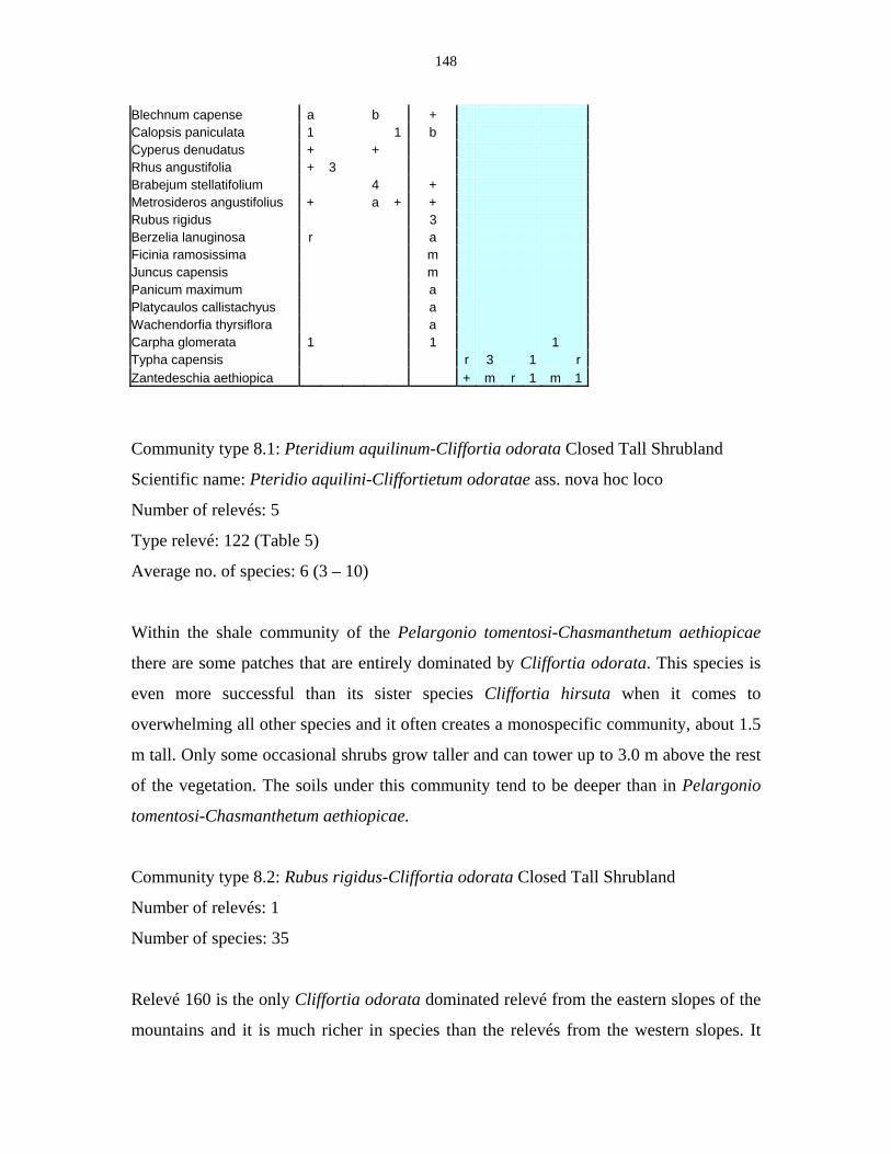
148
Blechnum capense a b + Calopsis paniculata 1 1 b Cyperus denudatus + + Rhus angustifolia + 3 Brabejum stellatifolium 4 + Metrosideros angustifolius + a + + Rubus rigidus 3 Berzelia lanuginosa r a Ficinia ramosissima m Juncus capensis m Panicum maximum a Platycaulos callistachyus a Wachendorfia thyrsiflora a Carpha glomerata 1 1 1 Typha capensis r 3 1 rZantedeschia aethiopica + m r 1 m 1
Community type 8.1: Pteridium aquilinum-Cliffortia odorata Closed Tall Shrubland
Scientific name: Pteridio aquilini-Cliffortietum odoratae ass. nova hoc loco
Number of relevés: 5
Type relevé: 122 (Table 5)
Average no. of species: 6 (3 – 10)
Within the shale community of the Pelargonio tomentosi-Chasmanthetum aethiopicae
there are some patches that are entirely dominated by Cliffortia odorata. This species is
even more successful than its sister species Cliffortia hirsuta when it comes to
overwhelming all other species and it often creates a monospecific community, about 1.5
m tall. Only some occasional shrubs grow taller and can tower up to 3.0 m above the rest
of the vegetation. The soils under this community tend to be deeper than in Pelargonio
tomentosi-Chasmanthetum aethiopicae.
Community type 8.2: Rubus rigidus-Cliffortia odorata Closed Tall Shrubland
Number of relevés: 1
Number of species: 35
Relevé 160 is the only Cliffortia odorata dominated relevé from the eastern slopes of the
mountains and it is much richer in species than the relevés from the western slopes. It
149
occurs in a very different habitat, namely on steep alluvial banks with a sandy soil. The
community is structurally more diverse than the previous community. Some of the
species present are: Calopsis paniculata, Carpha glomerata, Diospyros glabra,
Helichrysum helianthemifolium, Panicum maximum, Rubus rigidus, Stoebe plumosa and
Wachendorfia thyrsiflora.
Forest and Scrub communities (Appendix E; Table 6)
Forest and scrub communities have many species in common, yet they are different in
their syntaxonomic relationships. Scrub communities are typically riparian and the most
dominant species are restricted to the Fynbos Biome. Forests can occur in several
habitats, like screes or kloofs, and in some cases they can even cover entire mountain
slopes, as in the case of Table Mountain or the forests around Knysna. The forests in the
Fynbos Biome are of an Afromontane origin. This is the reason why the forest and scrub
communities are presented here as two separate entities in two different Community
groups. However, most scrub species can occur in riparian forest as well.
Community group 9
Forests in the Fynbos Biome are mainly restricted to kloofs, screes and riparian zones
(Campbell 1986b; Cowling et al. 1992; Manders et al. 1992). Many studies have been
done on forests in the Fynbos Biome (Campbell & Moll 1977; McKenzie et al. 1977;
Geldenhuys 1997). These forests are of an Afromontane origin and are most extensive in
the area around Knysna on the South Coast. Most species have an Afromontane
distribution and occur through the Drakensberg, Chimanimani Mountains to Mlanje in
Malawi. Some of the species, like Apodytes dimidiata, Ilex mitis, Podocarpus latifolius
and Rapanea melanophloeos, occur as far north as Ethiopia (White 1978).
In riparian forests some elements of riparian scrub occur together with the
Afromontane vegetation. Some of these species, such as Brabejum stellatifolium and
Metrosideros angustifolia, do not occur east of the Gouritz River (see Figure 2.12;
Campbell 1986b). In their study of the extensive forest communities of Table Mountain,
150
Campbell & Moll (1977) recognized a few forest communities that are typically riparian.
The single species that distinguishes riparian forest from other forest types is Cunonia
capensis (rooiels) and in some cases Platylophus trifoliatus (witels). These forests
typically occur on deeper soils and are most extensive in gorges that seldom burn. The
pH of the soil ranges between 4.5 and 5.0.
In this study, riparian forest was found in all the river catchments and, with the
exception of the communities typical for the Lourens River, there are not many
differences between the forests of the respective catchments. In most cases, forests occur
at low altitudes at the bottoms of the valleys, while structurally lower vegetation types
dominate at the higher altitudes. In Wesselsgat, in the Palmiet River catchment, this
situation is reversed, and one relevé in forest has been sampled here from above 800 m.
In the Riviersonderend and Boegoe Kloofs there are also some forest patches at high
altitudes. These gorges are very steep and probably receive a lot of rainfall. Protection
from fire and the moist climate will be the main reasons why the forests occur here.
Differential species of the Afromontane Forest in the tree layer are Apodytes dimidiata,
Cunonia capensis, Ilex mitis, Maytenus acuminata and Rapanea melanophloeos, while
the herb layer is dominated by Asparagus scandens, Hymenopeltatum peltatum and
Schoenoxiphium lanceum.
Community type 9.1: Platylophus trifoliatus-Cunonia capensis Forest
Number of relevés: 1
Number of species: 14
One relevé from Boesmanskloof is aberrant because it contains both Cunonia capensis
and Platylophus trifoliatus. In this locality not many samples have been taken, because it
is not an easily accessible area. The other dominant tree species is Brabejum
stellatifolium. The tree layer is the most important layer, but some large ferns of Todea
barbara occupy the herb layer. The community occurs in the Wet Bank Zone and some
typical Wet Bank species such as Pseudobaeckea africana occur in an open patch.
Community type 9.2: Platylophus trifoliatus Forest
151
Scientific name: Platylophietum trifoliati ass. novo hoc loco
Number of relevés: 4
Type relevé: 255 (Table 6)
Average no. of species: 9 (5 – 11)
This community occurs in the riparian belt of the Lourens River. The tree layer consists
of only one species: Platylophus trifoliatus. It grows on shallow mineral soils on a stony
bottom. The tree layer covers 80% of each sample, on average and grows to about 5 m
tall, while the herb layer is very sparse. Further up the bank it borders on a scree forest.
The only other community in which Platylophus trifoliatus dominates is the Platylophus
trifoliatus-Cunonia capensis Forest described above. This species also occurs
sporadically in Jonkershoek, but it does not form an extensive community there.
Community type 9.3: Curtisia dentata-Diospyros whyteana Scree Forest
Scientific name: Curtisio dentatae-Diospyretum whyteanae ass. nova hoc loco
Number of relevés: 5
Type relevé: 200 (Table 6)
Average no. of species: 15 (10 – 18)
This community occurs in the Back Dynamic Zone of the Lourens River. The tree layer
is the dominant stratum and it grows taller than in the former community, namely, up to 8
m tall. Common species are Ilex mitis, Kiggelaria africana, Maytenus acuminata, Olea
capensis and Rapanea melanophloeos while Curtisia dentata, Diospyros whyteana,
Podocarpus latifolius and possibly Olinia ventosa are differential. The herb layer is also
more extensive, but only covers about 20% of the sample area. A common grass species
in this layer is Ehrharta erecta, which is absent from most of the other forest types. This
is a typical scree forest and the only riparian characteristic is the occurrence of Cunonia
capensis. It might be that a scree forest is quite insensitive to flooding because the water
drains readily during a flood. That could explain why this vegetation type does not differ
much from the (non-riparian) scree forest types described by Campbell & Moll (1977) as
the Olea capensis-Curtisia dentata Variant. When the data from this study is compared
152
with the data of Campbell & Moll (1977), it appears that the Curtisio dentatae-
Diospyretum whyteanae is exactly the same as their community and it also matches a
community that was described by Boucher (1978). It appears to be that this is one of the
very few vegetation types in the Fynbos Biome that is widely distributed and that has
been well sampled. The community occurs on wet screes with shallow soils, intermediate
in organic matter.
McDonald (1988) describes another scree community from dry screes with
Heeria argentea and Rapanea melanophloeos as the dominant tree species.
Community type 9.4: Todea barbara-Cunonia capensis Forest
Scientific name: Todeo barbarae-Cunonietum capensis ass. nova hoc loco
Number of relevés: 25
Type relevé: 46 (Table 6)
Average no. of species: 17 (6 – 29)
This vegetation type forms the typical riparian forest found in the Western Cape
Province. Afromontane Forests, as the name implies, are not restricted to rivers and an
extensive study has been made of the forest types of Table Mountain by Campbell &
Moll (1977). In the Hottentots Holland Mountains, however, it is mainly restricted to
riparian habitats and wet kloofs. Only the forest vegetation of screes is a really distinct
riparian forest type (see the description of Curtisio dentatae-Diospyretum whyteanae). In
the Todeo barbarae-Cunonietum capensis there is much variation, which is best
described by subdividing the association into two subassociations. There are still some
unusual relevés, however, namely the relevés 18, 108, 112, 170, 209 and 211. Relevé 18
represents riparian scrub with one specimen of Ilex mitis in between, so it might be called
heterogeneous. Relevé 108 is located in a Wet Bank Zone that is forested. Relevé 112 is
dominated by young shrubs of Brabejum stellatifolium and it is transition between
Helichryso-Myrsinietum africanae inops and Todeo barbarae-Cunonietum capensis.
Relevé 170 is located on a steep riverbank and mostly contains low trees and shrubs.
Relevés 209 and 211 are very poor in species because they are sampled around a very
small and steep gully.
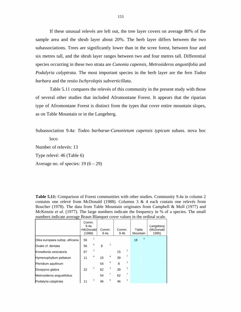
153
If these unusual relevés are left out, the tree layer covers on average 80% of the
sample area and the shrub layer about 20%. The herb layer differs between the two
subassociations. Trees are significantly lower than in the scree forest, between four and
six metres tall, and the shrub layer ranges between two and four metres tall. Differential
species occurring in these two strata are Cunonia capensis, Metrosideros angustifolia and
Podalyria calyptrata. The most important species in the herb layer are the fern Todea
barbara and the restio Ischyrolepis subverticillata.
Table 5.11 compares the relevés of this community in the present study with those
of several other studies that included Afromontane Forest. It appears that the riparian
type of Afromontane Forest is distinct from the types that cover entire mountain slopes,
as on Table Mountain or in the Langeberg.
Subassociation 9.4a: Todeo barbarae-Cunonietum capensis typicum subass. nova hoc
loco
Number of relevés: 13
Type relevé: 46 (Table 6)
Average no. of species: 19 (6 – 29)
Table 5.11: Comparison of Forest communities with other studies. Community 9.4a in column 2 contains one relevé from McDonald (1988). Columns 3 & 4 each contain one relevés from Boucher (1978). The data from Table Mountain originates from Campbell & Moll (1977) and McKenzie et al. (1977). The large numbers indicate the frequency in % of a species. The small numbers indicate average Braun Blanquet cover values in the ordinal scale.
Comm. 9.4a
+McDonald (1988)
Comm. 9.4a
Comm. 9.4b
Table Mountain
Langeberg (McDonald
1995)
Olea europaea subsp. africana 56 3 18 6
Oxalis cf. dentata 56 4 8 3
Knowltonia vesicatoria 67 3 15 2
Hymenophyllum peltatum 11 4 15 4 39 7
Pteridium aquilinum 54 6 8 2
Diospyros glabra 22 3 62 3 39 3
Metrosideros angustifolius 54 7 62 7
Podalyria calyptrata 11 3 46 6 46 5
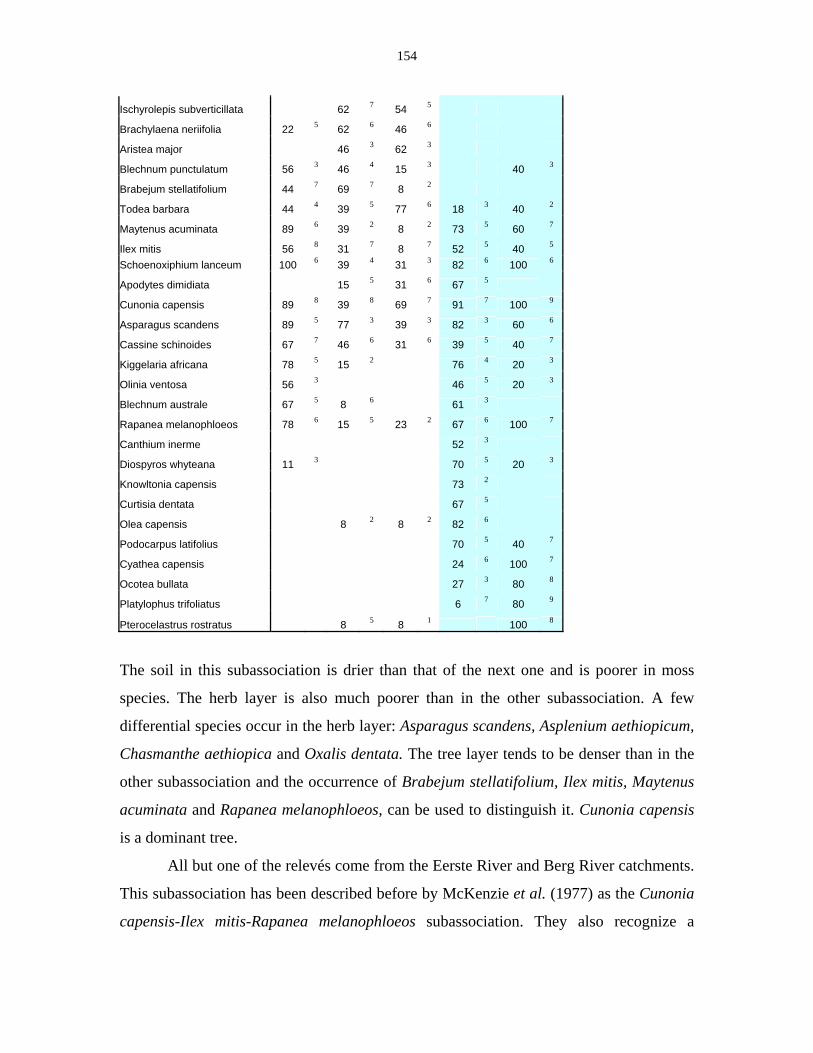
154
Ischyrolepis subverticillata 62 7 54 5
Brachylaena neriifolia 22 5 62 6 46 6
Aristea major 46 3 62 3
Blechnum punctulatum 56 3 46 4 15 3 40 3
Brabejum stellatifolium 44 7 69 7 8 2
Todea barbara 44 4 39 5 77 6 18 3 40 2
Maytenus acuminata 89 6 39 2 8 2 73 5 60 7
Ilex mitis 56 8 31 7 8 7 52 5 40 5 Schoenoxiphium lanceum 100 6 39 4 31 3 82 6 100 6
Apodytes dimidiata 15 5 31 6 67 5
Cunonia capensis 89 8 39 8 69 7 91 7 100 9
Asparagus scandens 89 5 77 3 39 3 82 3 60 6
Cassine schinoides 67 7 46 6 31 6 39 5 40 7
Kiggelaria africana 78 5 15 2 76 4 20 3
Olinia ventosa 56 3 46 5 20 3
Blechnum australe 67 5 8 6 61 3
Rapanea melanophloeos 78 6 15 5 23 2 67 6 100 7
Canthium inerme 52 3
Diospyros whyteana 11 3 70 5 20 3
Knowltonia capensis 73 2
Curtisia dentata 67 5
Olea capensis 8 2 8 2 82 6
Podocarpus latifolius 70 5 40 7
Cyathea capensis 24 6 100 7
Ocotea bullata 27 3 80 8
Platylophus trifoliatus 6 7 80 9
Pterocelastrus rostratus 8 5 8 1 100 8
The soil in this subassociation is drier than that of the next one and is poorer in moss
species. The herb layer is also much poorer than in the other subassociation. A few
differential species occur in the herb layer: Asparagus scandens, Asplenium aethiopicum,
Chasmanthe aethiopica and Oxalis dentata. The tree layer tends to be denser than in the
other subassociation and the occurrence of Brabejum stellatifolium, Ilex mitis, Maytenus
acuminata and Rapanea melanophloeos, can be used to distinguish it. Cunonia capensis
is a dominant tree.
All but one of the relevés come from the Eerste River and Berg River catchments.
This subassociation has been described before by McKenzie et al. (1977) as the Cunonia
capensis-Ilex mitis-Rapanea melanophloeos subassociation. They also recognize a
155
related community without Rapanea melanophloeos that was also recognized by
Campbell & Moll (1977). This Cunonia capensis-Ilex mitis Community will occur in
drier situations than the former. In the Hottentots Holland Mountains this community was
not distinguished. Boucher (1978) found the Cunonia-Alsophila Kloof Forest, which is
definitely different from the type described here.
In this study it was found that the forests in Jonkershoek are often co-dominated
(except for one aberrant sample where it is the dominant species) by Brabejum
stellatifolium. Werger et al. (1972) described this community as Rapanea melanophloeos
Community. This is the same as McDonald’s (1988) Rapanea melanophloeos-Cunonia
capensis High Forest. It is found on mineral soils that contain many boulders. The
substrate can be either granite or sandstone.
Subassociation 9.4b: Todeo barbarae-Cunonietum capensis hymenophylletosum peltatae
subass. nova hoc loco
Number of relevés: 12
Type relevé: 64 (Table 6)
Average no. of species: 18 (6 – 29)
This subassociation is poorer in species than the first one, but has a higher cover of the
herb layer. The soils are wetter and they support more mosses and the fern
Hymenophyllum peltatum, which grows in the moss layer. This species attains a high
cover on wet, vertical slopes. The herb layer covers 40% on average and the moss layer
30%. Differential species in the herb layer are Aristea major, Elaphoglossum angustatum
and Hymenophyllum peltatum. Many of the relevés were sampled from steep slopes in
ravines. The subassociation appears to be a transition between Afromontane Forest and
the riverine Scrub communities of Community Group 10 because it also contains typical
species from that group, such as Brachylaena neriifolia and Metrosideros angustifolia.
The ground layer is dominated by Todea barbara and Ischyrolepis subverticillata.
Compared with the subassociation typicum, it will be closer to Boucher’s (1978)
Cunonia-Alsophila Kloof Forest. However, the tree fern Cyathea capensis, an important
species in his community, was only found in one sample in the Hottentots Holland area.
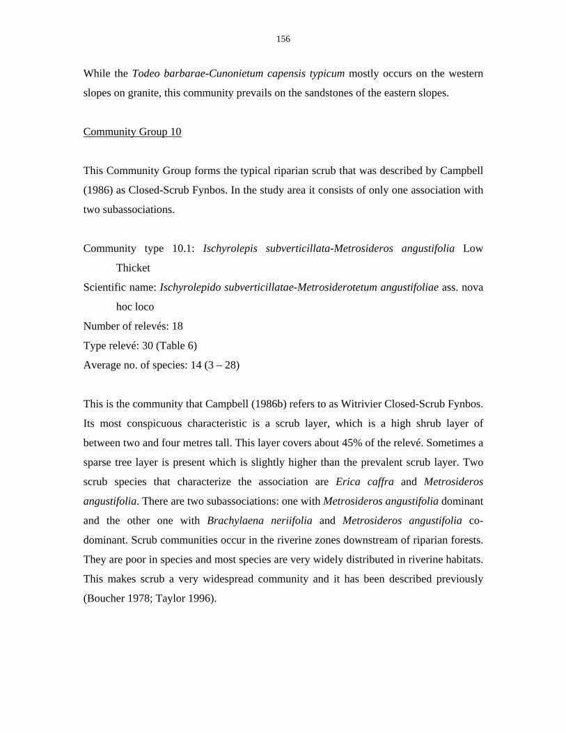
156
While the Todeo barbarae-Cunonietum capensis typicum mostly occurs on the western
slopes on granite, this community prevails on the sandstones of the eastern slopes.
Community Group 10
This Community Group forms the typical riparian scrub that was described by Campbell
(1986) as Closed-Scrub Fynbos. In the study area it consists of only one association with
two subassociations.
Community type 10.1: Ischyrolepis subverticillata-Metrosideros angustifolia Low
Thicket
Scientific name: Ischyrolepido subverticillatae-Metrosiderotetum angustifoliae ass. nova
hoc loco
Number of relevés: 18
Type relevé: 30 (Table 6)
Average no. of species: 14 (3 – 28)
This is the community that Campbell (1986b) refers to as Witrivier Closed-Scrub Fynbos.
Its most conspicuous characteristic is a scrub layer, which is a high shrub layer of
between two and four metres tall. This layer covers about 45% of the relevé. Sometimes a
sparse tree layer is present which is slightly higher than the prevalent scrub layer. Two
scrub species that characterize the association are Erica caffra and Metrosideros
angustifolia. There are two subassociations: one with Metrosideros angustifolia dominant
and the other one with Brachylaena neriifolia and Metrosideros angustifolia co-
dominant. Scrub communities occur in the riverine zones downstream of riparian forests.
They are poor in species and most species are very widely distributed in riverine habitats.
This makes scrub a very widespread community and it has been described previously
(Boucher 1978; Taylor 1996).
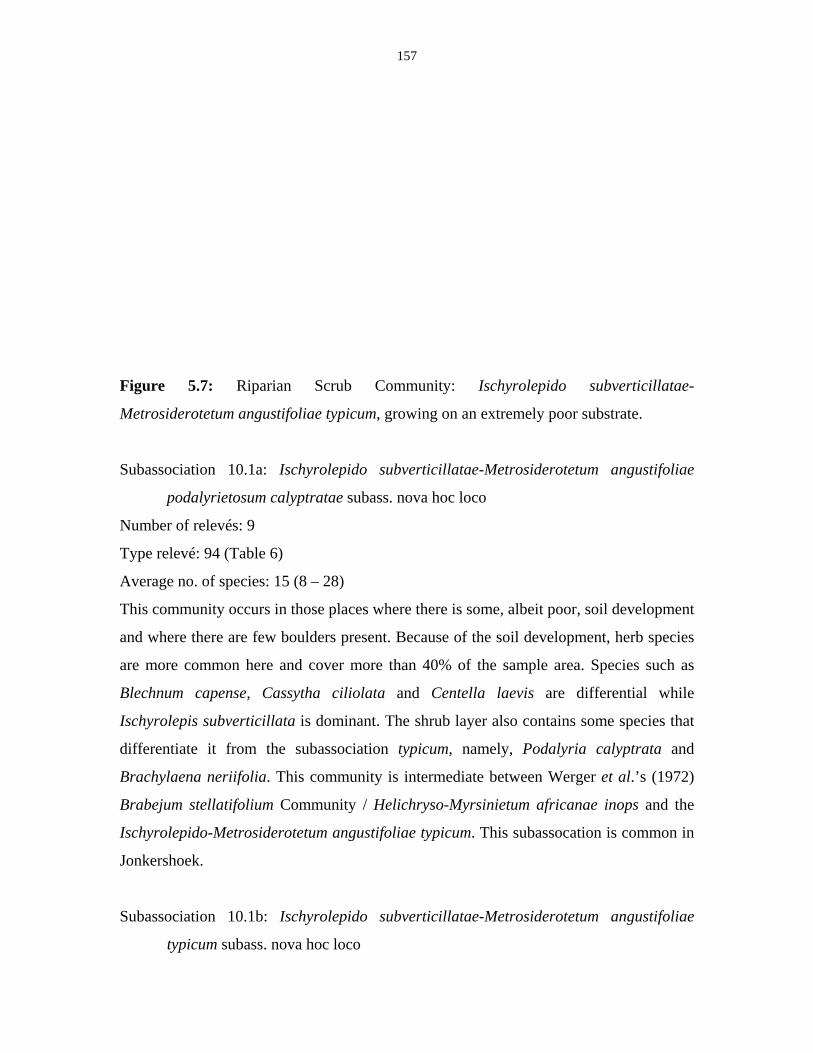
157
Figure 5.7: Riparian Scrub Community: Ischyrolepido subverticillatae-
Metrosiderotetum angustifoliae typicum, growing on an extremely poor substrate.
Subassociation 10.1a: Ischyrolepido subverticillatae-Metrosiderotetum angustifoliae
podalyrietosum calyptratae subass. nova hoc loco
Number of relevés: 9
Type relevé: 94 (Table 6)
Average no. of species: 15 (8 – 28)
This community occurs in those places where there is some, albeit poor, soil development
and where there are few boulders present. Because of the soil development, herb species
are more common here and cover more than 40% of the sample area. Species such as
Blechnum capense, Cassytha ciliolata and Centella laevis are differential while
Ischyrolepis subverticillata is dominant. The shrub layer also contains some species that
differentiate it from the subassociation typicum, namely, Podalyria calyptrata and
Brachylaena neriifolia. This community is intermediate between Werger et al.’s (1972)
Brabejum stellatifolium Community / Helichryso-Myrsinietum africanae inops and the
Ischyrolepido-Metrosiderotetum angustifoliae typicum. This subassocation is common in
Jonkershoek.
Subassociation 10.1b: Ischyrolepido subverticillatae-Metrosiderotetum angustifoliae
typicum subass. nova hoc loco
158
Number of relevés: 9
Type relevé: 30 (Table 6)
Average no. of species: 11 (3 – 19)
This community grows in those situations where the riverbed is very stony and soil
development is extremely poor. Stream power is likely to be very strong during a flood.
Only very few species survive in this habitat and Metrosideros angustifolia is the most
successful among them, which results in a dominance by this species. The herb layer is
mostly occupied by Todea barbara and Ischyrolepis subverticillata, but does not reach a
high cover. This subassociation is particularly common in Assegaaibosch Kloof.
5.9 Discussion
The proposed classification of riverine vegetation is summarized in Table 5.12. Each of
the Community Groups has its own diagnostic species, which have been presented above
in all the descriptions of the Community Groups. There are however also very common
species that occur across the Community Groups. Many of these are typically riparian,
others are just very common Fynbos elements. They can be seen in the last rows
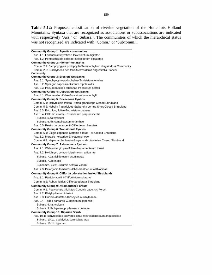
159
Table 5.12: Proposed classification of riverine vegetation of the Hottentots Holland Mountains. Syntaxa that are recognized as associations or subassociations are indicated with respectively ‘Ass.’ or ‘Subass.’. The communities of which the hierarchical status was not recognized are indicated with ‘Comm.’ or ‘Subcomm.’. Community Group 1: Aquatic communities Ass. 1.1: Fontinali antipyreticae-Isolepidetum digitatae Ass. 1.2: Pentaschistido pallidae-Isolepidetum digiatatae Community Group 2: Pioneer Wet Banks Comm. 2.1: Symphyogyna podophylla-Sematophyllum dregei Moss Community Comm. 2.2: Brachylaena neriifolia-Metrosideros angustifolia Pioneer Community Community Group 3: Erosion Wet Banks Ass. 3.1: Symphyogyno podophyllae-Schizietum tenellae Ass. 3.2: Sphagno capensis-Disetum tripetaloidis Ass. 3.3: Pseudobaeckeo africanae-Prionietum serrati Community Group 4: Deposition Wet Banks Ass. 4.1: Wimmerello bifidae-Juncetum lomatophylli Community Group 5: Ericaceous Fynbos Comm. 5.1: Ischyrolepis triflora-Protea grandiceps Closed Shrubland Comm. 5.2: Nebelia fragarioides-Staberoha cernua Short Closed Shrubland Ass. 5.3: Erico longifoliae-Tetrarietum crassae Ass. 5.4: Cliffortio atratae-Restionetum purpurascentis Subass. 5.4a: typicum Subass. 5.4b: centelletosum erianthae Ass. 5.5: Restio purpurascenti-Cliffortietum hirsutae Community Group 6: Transitional Fynbos Comm. 6.1: Elegia capensis-Cliffortia hirsuta Tall Closed Shrubland Ass. 6.2: Muraltio heisteriae-Ericetum pineae Comm. 6.3: Haplocarpha lanata-Euryops abrotanifolius Closed Shrubland Community Group 7: Asteraceous Fynbos Ass. 7.1: Wahlenbergio parvifoliae-Pentameritetum thuarii Ass. 7.2: Helichryso cymosi-Myrsinietum africanae Subass. 7.2a: ficinietosum acuminatae Subass. 7.2b: inops Subcomm. 7.2c: Cullumia setosia Variant Ass. 7.3: Pelargonio tomentosi-Chasmanthetum aethiopicae Community Group 8: Cliffortia odorata dominated Shrublands Ass. 8.1: Pteridio aquilini-Cliffortietum odoratae Comm. 8.2: Rubus rigidus-Cliffortia odorata Shrubland Community Group 9: Afromontane Forests Comm. 9.1: Platylophus trifoliatus-Cunonia capensis Forest Ass. 9.2: Platylophietum trifoliati Ass. 9.3: Curtisio dentatae-Diospyretum whyteanae Ass. 9.4: Todeo barbarae-Cunonietum capensis Subass. 9.4a: typicum Subass. 9.4b: hymenophylletosum peltatae Community Group 10: Riparian Scrub Ass. 10.1: Ischyrolepido subverticillatae-Metrosiderotetum angustifoliae Subass. 10.1a: podalyrietosum calyptratae Subass. 10.1b: typicum
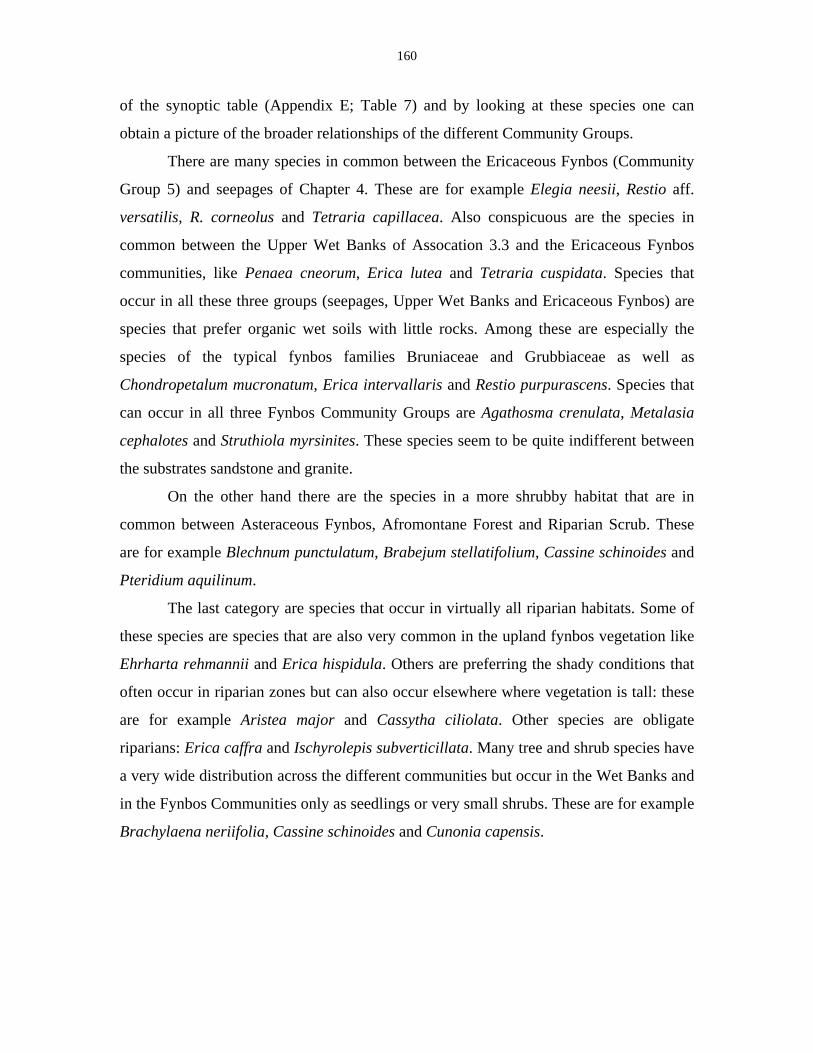
160
of the synoptic table (Appendix E; Table 7) and by looking at these species one can
obtain a picture of the broader relationships of the different Community Groups.
There are many species in common between the Ericaceous Fynbos (Community
Group 5) and seepages of Chapter 4. These are for example Elegia neesii, Restio aff.
versatilis, R. corneolus and Tetraria capillacea. Also conspicuous are the species in
common between the Upper Wet Banks of Assocation 3.3 and the Ericaceous Fynbos
communities, like Penaea cneorum, Erica lutea and Tetraria cuspidata. Species that
occur in all these three groups (seepages, Upper Wet Banks and Ericaceous Fynbos) are
species that prefer organic wet soils with little rocks. Among these are especially the
species of the typical fynbos families Bruniaceae and Grubbiaceae as well as
Chondropetalum mucronatum, Erica intervallaris and Restio purpurascens. Species that
can occur in all three Fynbos Community Groups are Agathosma crenulata, Metalasia
cephalotes and Struthiola myrsinites. These species seem to be quite indifferent between
the substrates sandstone and granite.
On the other hand there are the species in a more shrubby habitat that are in
common between Asteraceous Fynbos, Afromontane Forest and Riparian Scrub. These
are for example Blechnum punctulatum, Brabejum stellatifolium, Cassine schinoides and
Pteridium aquilinum.
The last category are species that occur in virtually all riparian habitats. Some of
these species are species that are also very common in the upland fynbos vegetation like
Ehrharta rehmannii and Erica hispidula. Others are preferring the shady conditions that
often occur in riparian zones but can also occur elsewhere where vegetation is tall: these
are for example Aristea major and Cassytha ciliolata. Other species are obligate
riparians: Erica caffra and Ischyrolepis subverticillata. Many tree and shrub species have
a very wide distribution across the different communities but occur in the Wet Banks and
in the Fynbos Communities only as seedlings or very small shrubs. These are for example
Brachylaena neriifolia, Cassine schinoides and Cunonia capensis.
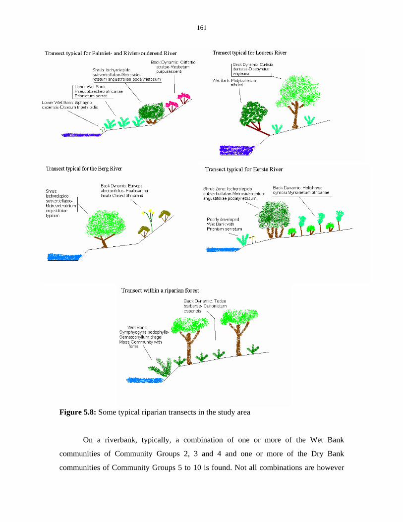
161
Figure 5.8: Some typical riparian transects in the study area
On a riverbank, typically, a combination of one or more of the Wet Bank
communities of Community Groups 2, 3 and 4 and one or more of the Dry Bank
communities of Community Groups 5 to 10 is found. Not all combinations are however
162
likely to occur. Except for a classification of vegetation types, a classification of
riverbanks is possible if one looks at the combination of vegetation types. The river
banks illustrated in Figure 5.9 are the most important of these, but there are many
variations on these and there are also less common types like the river banks on
Malmesbury shale (with communities 7.3 and 8.2 in the Dry Bank and poorly developed
Wet Banks), river banks with seepage from the slopes (with communities 5.5 and 6.1 in
the Dry Bank and communities of Community Group 3 in the Wet Banks) or river banks
where deposition dominates and sand beaches develop (with community 4.1 in the Wet
Bank and community 10.1a in the Dry Bank).
The TWINSPAN analysis, the Correspondence Analysis and the hierarchical
clustering using SYNTAX all showed similar results about the basic clustering of the
data on riparian vegetation collected in this study. It is only when vegetation types are
compared with other studies in the Fynbos Biome that clusters become differently
defined. This is mainly because some aberrant samples fit in better with the other studies.
The best way to improve the present classification is to collect more data, especially from
other areas in the biome. The use of the Community Groups is sufficient at this stage.
In the comparison with the other types it also has become clear which vegetation
types were under- or oversampled. The only well sampled vegetation type in the study
has been the Curtisio dentatae-Diospyretum whyteana, since detailed vegetation data on
this type has already been collected by Campbell & Moll (1977) and by Boucher (1978).
Vegetation sampling in forests is easier than in fynbos, because the species are more
widespread and easily identified. The different Wet Bank types in this study have also
been well sampled and the sufficient amount of data has helped to define them
adequately. From what I have seen outside Hottentots Holland, I do not expect a high
regional variation in these vegetation types either. The vegetation types that need to be
sampled further are the Fynbos communities. These communities have a high regional
diversity and show a completely different species composition in other mountain ranges.
Although there is one Riparian Fynbos type in the Hottentots Holland Mountains that is
clearly dominant (Cliffortio atratae-Restionetum purpurascentis), there are still some
types with narrow distribution ranges (but not necessarily so in other mountain ranges)
that are undersampled.
163
More data from other river catchments within the biome should be collected
before attention should be directed to a comprehensive hierarchical classification. The
distribution of the different riparian vegetation types through the Fynbos Biome must be
determined before any conclusions can be drawn about rarity and uniqueness of the
vegetation types. Some rare vegetation types recorded in the Hottentots Holland
Mountains might be more common in other places in the Fynbos Biome. However,
because the Hottentots Holland Mountain Range is the wettest area of the Biome and
perennial rivers become scarcer further to the north and to the east, this is not very likely
to be the case for most vegetation types. Dominant species in the present study like
Restio purpurascens only have a limited distribution outside the study area. It is quite
probable that rare vegetation types within this study are also rare vegetation types
throughout the Fynbos Biome, such as, for example, the Cliffortia hirsuta dominated
shrublands or the Muraltio heisteriae-Ericetum pineae. Perhaps the most unique
vegetation types found in this study are those from the granites and shales, because these
substrates are relatively rare in the mountains of the Fynbos Biome. The Pelargonio
tomentosi-Chasmathetum aethiopicae was only found in one locality and it is quite
improbable that a similar vegetation type will be found elsewhere, because it is entirely
restricted to the unusual occurrence of shales from the Malmesbury Group in the
mountains.
The vegetation types that are found in this study can be used to identify the river
zonation. All the types are characteristic for a specific zone on the riverbank and
vegetation types can be used to determine the hydrological regime. This also means that
changes will occur in the vegetation after changes occur in the flood regime. This implies
that changes in the flood regime can be assessed by monitoring riparian vegetation types.
The following chapter will deal in detail with the links between vegetation and channel
hydraulics.
The collection of data in the mountains is always more difficult than in the
lowlands because of access difficulties. However, in a river ecosystem, the ecological
processes in the mountain reaches are intricately correlated with those in the lowlands,
because the entire river catchment can be seen as one ecosystem. Riparian vegetation
should be monitored in all the reaches, because only then a complete overview of the

164
state of the river can be achieved. With this survey of twenty-six communities and five
subcommunities of which eighteen were recognized as an association, a contribution
towards this aim has been achieved.
165
6. The influence of floods on the vegetation zonation along mountain
streams in the Western Cape
E.J.J. Sieben, G.R. Basson*, J.G. Malan* & C. Boucher
* Department of Civil Engineering, University of Stellenbosch, Private Bag X1, Matieland 7602
Keywords: Hydrology, hydraulics, riparian vegetation, mountain streams, floods, stream
power, Manning’s n.
6.1 Abstract
In this paper we aim to describe zonation patterns of riparian vegetation in mountain
streams using hydraulic and hydrological parameters. Flow data is not available at the
sites used in the study, because all sites are situated upstream from the existing weirs.
The discharge data at the weirs is extrapolated to the sites upstream by multiplication
with a correction factor that is dependent on the size of the subcatchment. In this way,
recurrence intervals for floods in mountain streams are derived. Discharges at sites are
also calculated using bed roughness or Manning’s n in straight sections with uniform
flow conditions. Stream power is derived from the discharges calculated in this manner.
The combination of stream power and recurrence intervals explains the occurrence of
most vegetation types occurring on the banks, except for one type: Afromontane Forest.
This type is more dependent on other factors, such as protection from fire and the depth
of the groundwater table.
6.2 Introduction Riparian plants are highly influenced by the fluctuations in the water level of the river
and especially by large flood events (Menges & Waller 1983; Hupp 1988). While small
annual floods are important to keep a narrow vegetation zone next to the river wet and to
determine small-scale processes such as germination and seedling survival, larger floods,
that occur less than once a year, have a major impact on the riparian zones higher up the
riverbank. They can uproot trees and shrubs and move boulders in the riverbed and create
166
large habitat structures such as oxbow lakes. Flood events occur in a continuum from
low-power, high frequency floods to high-power, low frequency floods. Inundation
frequency and stream power are often assumed to be inversely proportional (Brinson
1990; Naiman & Décamps 1997). A detailed study of stream power by Bendix (1999)
shows that this assumption is not necessarily correct and that stream power has its own
influence independent of inundation frequency. This impact varies between different
catchments because the effect of stream power is dependent on local geomorphology. In
steep gorges, stream power is generally greater than in wide valleys.
The impact of large floods on vegetation can be seen best by the impact of
impoundments on the downstream riparian vegetation. In the case of impoundment,
large flood events are retarded or reduced and riparian vegetation on floodplains and
higher riverbanks starts to change (Stevens et al. 1995; Trémolières et al. 1998; Dixon &
Johnson 1999). The impact of large dams on downstream biota is best described by Ward
& Stanford (1979).
In South Africa, where nearly every river is impounded in at least one place, and
water shortage is a realistic threat (Davies & Day 1998), a methodology has been
developed to calculate the minimum requirements for environmental flows (King et al.
2000). This is called the Building Block Methodology and it has been successfully
applied, for example, in studies in Lesotho (Metsi Consultants 1999) and on the Palmiet
River in the Western Cape (Brown & Day 1998). For the calculation of the Instream
Flow Requirements of these rivers information about the correlation between flood
regimes and riparian vegetation is fundamental, and to this end the lower reaches of these
rivers have been studied in some detail. A problem arises when studying mountain
streams upstream of the dams because few flow data are available in these reaches. The
flood regime here is still in its original state but the vegetation is different from that
found in the lower reaches of the respective rivers. For a full understanding of the
riverine ecosystem these reaches need further study.
Riverbanks in the higher reaches of rivers are of the stenosaleutic type (Kopecky
1969). This means that the banks are steep, bank zonation is compressed and annual
flood level fluctuations are typically less than one meter. The heights of upstream floods
are correlated to the height of the downstream floods, but it is not known with what
167
factor they are correlated. This depends on the size of the catchment, the rainfall within
the catchment and the runoff from the catchment.
6.3 Aim of study
In this study we aim to describe riparian vegetation patterns by using hydraulic and
hydrological parameters in ungauged mountain catchments. The riparian vegetation in
these mountain streams shows clear zonation patterns and flood influences are clearly
visible in the vegetation. Hydraulic data consists of zone heights above the riverbed,
longitudinal slopes of the river and total input stream power. These data are compared
with the data available from the hydrological approach, which consists of an
extrapolation upstream of the flow discharges, and the frequencies of floods that are
measured at a weir downstream.
6.4 Study area
Two mountain catchments in the Western Cape were chosen to survey the flood events in
riparian vegetation of mountain streams. Both are situated in the Hottentots Holland
Nature Reserve but they have different exposures and different geological substrates. The
data from the weirs in the catchment was kindly placed at our disposal by the Department
of Water Affairs (Department of Water Affairs and Forestry, unpublished data).
The Eerste River Catchment is found in the western section of the Hottentots
Holland Mountain range. The bottom of the valley is underlain by granite, while the
highest reaches of the rivers start on Table Mountain Group sandstone. The weir G2H008
is located immediately upstream of the Kleinplaas Dam and has a 40 year flow record,
from 1961 to 2000. The area of the catchment above this weir is about 25 km2
(Department of Water Affairs and Forestry, unpublished data).
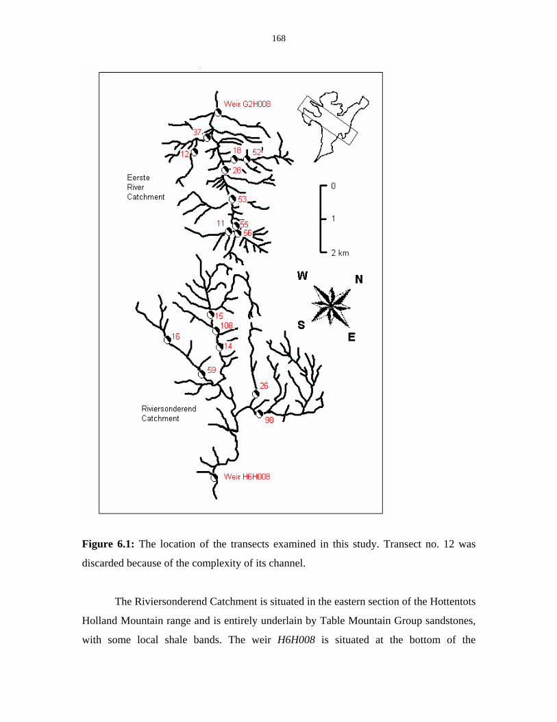
168
Figure 6.1: The location of the transects examined in this study. Transect no. 12 was
discarded because of the complexity of its channel.
The Riviersonderend Catchment is situated in the eastern section of the Hottentots
Holland Mountain range and is entirely underlain by Table Mountain Group sandstones,
with some local shale bands. The weir H6H008 is situated at the bottom of the
169
Riviersonderend Kloof, just before the Riviersonderend River enters the Theewaterskloof
Dam. The weir has a flow record of 29 years, from 1963 to 1992. Above the weir the
river drains an area of about 38 km2 (Department of Water Affairs and Forestry,
unpublished data). 6.5 Methods
Seventeen transects were chosen in both catchments: Two at the weirs H6H008 and
G2H008, eight dispersed through the Eerste River Catchment above the weir and seven
in the Riviersonderend Catchment above the weir. Figure 6.1 indicates the location of the
transects within the catchments.
In every transect a profile through the riverbed was measured using a Vertex
Forestor hypsometer. Vegetation on one bank was sampled (in the transects near the
weirs both banks were sampled) and characterized using the Braun-Blanquet method
(Westhoff & Van der Maarel 1973; Werger 1974). Flood heights that are required to
submerge specific vegetation zones can be derived from these profiles and are then
translated into discharges. This is possible using a discharge table. Only three observed
points are needed in such a discharge table (Gordon et al. 1992) and other data can be
derived through interpolation. The discharges at these points can be calculated in two
different ways (see below).
The realistic flood levels and their frequencies are derived from the flow records
at the downstream weir. Although rainfall is not equally distributed over the whole
catchment, it is assumed that the magnitude of a flood at a certain point is directly
correlated to the square root of the size of the subcatchment that it drains. The
magnitudes of the interannual floods are derived from the record of yearly peak flows at
the weir. In the table below the sizes of the peak flows for the two weirs are shown.
6.6 Analysis
The method of calculating the discharge at a particular transect in the catchment from the
flow depth depends on the local situation. The flows in mountain streams are generally

170
subcritical flows which means that they are controlled by a critical point such as a
cascade immediately downstream. This means that at the critical point the flow goes
through a critical depth, which changes the flow to supercritical. Sub- and supercritical
flows simply represent the two different states of flow possible for a certain net energy
level: subcritical representing the lower velocity, deeper flow state, and supercritical
representing a higher velocity, shallower flow state. If this critical point or cascade is
nearby and forms a simple channel (as in a weir), it can be used as a control section. The
discharge can be calculated from the control section because the discharge here will be
the same as in the original section. Certain unique characteristics are found at the control
section making it possible to calculate the discharge there if the critical depth is known.
This method of deriving the discharge has been used in four transects: Transect 11 and 28
in the Eerste River and Transect 15 and 26 in the Riviersonderend River. However, it
appeared that this method is quite sensitive to certain variables that had to be estimated
and it was abandoned at a later stage.
At the critical point of a cascade the following equation is valid:
13
2
=⋅
⋅
c
top
Ag
BQ (1)
In which Q is the discharge, Btop is the top width of the river at a certain water depth, g is
the acceleration of gravity and Ac is the cross-sectional area of the water (Featherstone &
Nalluri 1995). From this equation the discharge can be calculated if Ac is known. To
relate this to the water depth at the point of sampling slightly upstream, the equal-energy
equation can be used, assuming that the discharge is equal at both points:
22
2
222
2
22 AgQyz
AgQyz
ccc ⋅⋅
++=⋅⋅
++ (2)
where z is the elevation of the riverbed in relation to a fixed level and y the depth of the
water at both points. Equations (1) and (2) can be solved simultaneously through repeated
171
iteration to determine the two unknown variables, discharge Q and water depth y2
(Featherstone & Nalluri 1995). The problem with this method is that the value of z2 has
to be determined very accurately. The hypsometer did not allow this precision so the
value had to be estimated, which left many insecurities in the results. The method was
abandoned at a later stage.
After the first method was abandoned, the second method was applied to all
transects. In this method, the discharge has to be calculated directly from the flow depth
related to a vegetation zone at the spot. One factor complicating this calculation is the
hydraulic roughness of the streambed. The hydraulic roughness of the streambed is
dependent on the shape of the bed sediments that cause resistance to the flow. If
streamflow is low and many boulders stick above the water surface, the flow will have a
lot of resistance and relative roughness will increase as flows get smaller. On the other
hand, if flows get so large that the riparian vegetation is completely submerged, hydraulic
roughness increases as well. In mountain streams, hydraulic roughness is generally much
greater than in the lower reaches because of the coarse bed material, steep slopes and
dense riparian vegetation containing a large woody component. This makes accurate flow
calculations difficult, as most of the available formulae are not scientifically sound under
low-flow or high roughness conditions.
In a situation with relatively straight sections with uniform flow conditions the discharge
Q can be calculated using the Manning’s friction equation:
nSRAQ ⋅⋅
=3
2
(3)
In which R is the hydraulic radius (Area / wetted perimeter), S is the slope and n is
Manning’s n value expressing the hydraulic roughness of the riverbed (Featherstone &
Nalluri 1995). Roughness is a difficult value to determine (Gordon et al. 1992). In this
study the following formula has been used:
172
6139.0
85.0
50
84
46.0
84
11.11 Rsdd
dRg
n ⎪⎭
⎪⎬⎫
⎪⎩
⎪⎨⎧
⋅⎟⎟⎠
⎞⎜⎜⎝
⎛⋅⎟⎟
⎠
⎞⎜⎜⎝
⎛⋅⋅= −
−
(4)
in which d50 is the average boulder size in the river bed and d84 the 84 percentile boulder
size (Simons & Senturk 1992). The roughness is calculated separately for the riverbed
and the banks, because the riparian vegetation has a high impact on the roughness. For
this purpose the river profile has been subdivided into three sections, in which the two
bank sections have a maximum roughness. Application of this formula to the
mountainous reaches of the Eerste and Riviersonderend Rivers shows that Manning’s n
varies between values of 0.15 and 0.25. These are problematic values because they mean
extreme roughness and many of the flow equations do not apply in this situation.
Flood levels at the weirs
The discharge data for the weirs G2H008 and H6H008 were supplied by the Department
of Water Affairs and Forestry. The peak discharges at H6H008 were all above the
maximum of the weir discharge capacity, which is only designed to register small flood
events. These discharges were then calculated from the peak flood levels (h) by
extrapolation of the discharge tables. The equation used for this extrapolation was:
( )BDhAQ +⋅= (5)
in which A was calibrated as 46.8427, B as 0.41448 and D as -1.12.
From the annual peak discharges of the two rivers the discharges for several recurrence
intervals at the weir can be calculated. For this purpose the program STFLOOD
(Alexander 1991) was used. The results of this analysis are shown in Table 6.1.

173
Table 6.1: Floods at the different recurrence intervals at the weirs
Recurrence
Interval (year)
Eerste River
G2H008
Riviersonderend
H6H008
1 yr 30 m3/s 44 m3/s
2 yr 37.5 m3/s 50 m3/s
5 yr 50 m3/s 54 m3/s
10 yr 56.5 m3/s 56 m3/s
20 yr 64 m3/s 58 m3/s
50 yr 73 m3/s 60 m3/s
The discharges of these recurrence intervals occurring at the transects in the higher
reaches are correlated to the discharges at the weir through the proportion of the
catchment that they drain. To calculate the discharges for these same recurrence intervals
at the transects this area-effect can be accounted for by the following formula:
weirttran QAAQ ⋅= 1
sec (6)
where A1 represents the surface area of the subcatchment drained by the transect and A
the surface area of the entire catchment (Alexander 1991).
Surface areas of the subcatchments were calculated with the help of the WaterShed
command of the Geographic Information System IDRISI (Eastman 1997) and a Digital
Elevation Model of the area, which was supplied by the Western Cape Nature
Conservation Board.
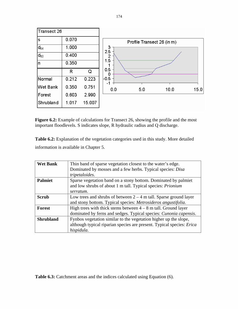
174
Figure 6.2: Example of calculations for Transect 26, showing the profile and the most important floodlevels. S indicates slope, R hydraulic radius and Q discharge.
Table 6.2: Explanation of the vegetation categories used in this study. More detailed
information is available in Chapter 5.
Wet Bank Thin band of sparse vegetation closest to the water’s edge. Dominated by mosses and a few herbs. Typical species: Disa tripetaloides.
Palmiet Sparse vegetation band on a stony bottom. Dominated by palmiet and low shrubs of about 1 m tall. Typical species: Prionium serratum.
Scrub Low trees and shrubs of between 2 – 4 m tall. Sparse ground layer and stony bottom. Typical species: Metrosideros angustifolia.
Forest High trees with thick stems between 4 – 8 m tall. Ground layer dominated by ferns and sedges. Typical species: Cunonia capensis.
Shrubland Fynbos vegetation similar to the vegetation higher up the slope, although typical riparian species are present. Typical species: Erica hispidula.
Table 6.3: Catchment areas and the indices calculated using Equation (6).
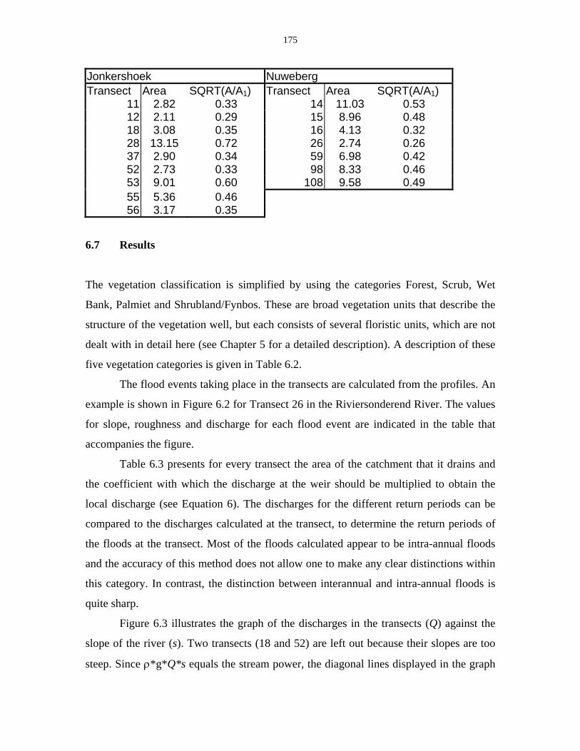
175
Jonkershoek Nuweberg Transect Area SQRT(A/A1) Transect Area SQRT(A/A1)
11 2.82 0.33 14 11.03 0.53 12 2.11 0.29 15 8.96 0.48 18 3.08 0.35 16 4.13 0.32 28 13.15 0.72 26 2.74 0.26 37 2.90 0.34 59 6.98 0.42 52 2.73 0.33 98 8.33 0.46 53 9.01 0.60 108 9.58 0.49 55 5.36 0.46 56 3.17 0.35
6.7 Results
The vegetation classification is simplified by using the categories Forest, Scrub, Wet
Bank, Palmiet and Shrubland/Fynbos. These are broad vegetation units that describe the
structure of the vegetation well, but each consists of several floristic units, which are not
dealt with in detail here (see Chapter 5 for a detailed description). A description of these
five vegetation categories is given in Table 6.2.
The flood events taking place in the transects are calculated from the profiles. An
example is shown in Figure 6.2 for Transect 26 in the Riviersonderend River. The values
for slope, roughness and discharge for each flood event are indicated in the table that
accompanies the figure.
Table 6.3 presents for every transect the area of the catchment that it drains and
the coefficient with which the discharge at the weir should be multiplied to obtain the
local discharge (see Equation 6). The discharges for the different return periods can be
compared to the discharges calculated at the transect, to determine the return periods of
the floods at the transect. Most of the floods calculated appear to be intra-annual floods
and the accuracy of this method does not allow one to make any clear distinctions within
this category. In contrast, the distinction between interannual and intra-annual floods is
quite sharp.
Figure 6.3 illustrates the graph of the discharges in the transects (Q) against the
slope of the river (s). Two transects (18 and 52) are left out because their slopes are too
steep. Since ρ*g*Q*s equals the stream power, the diagonal lines displayed in the graph
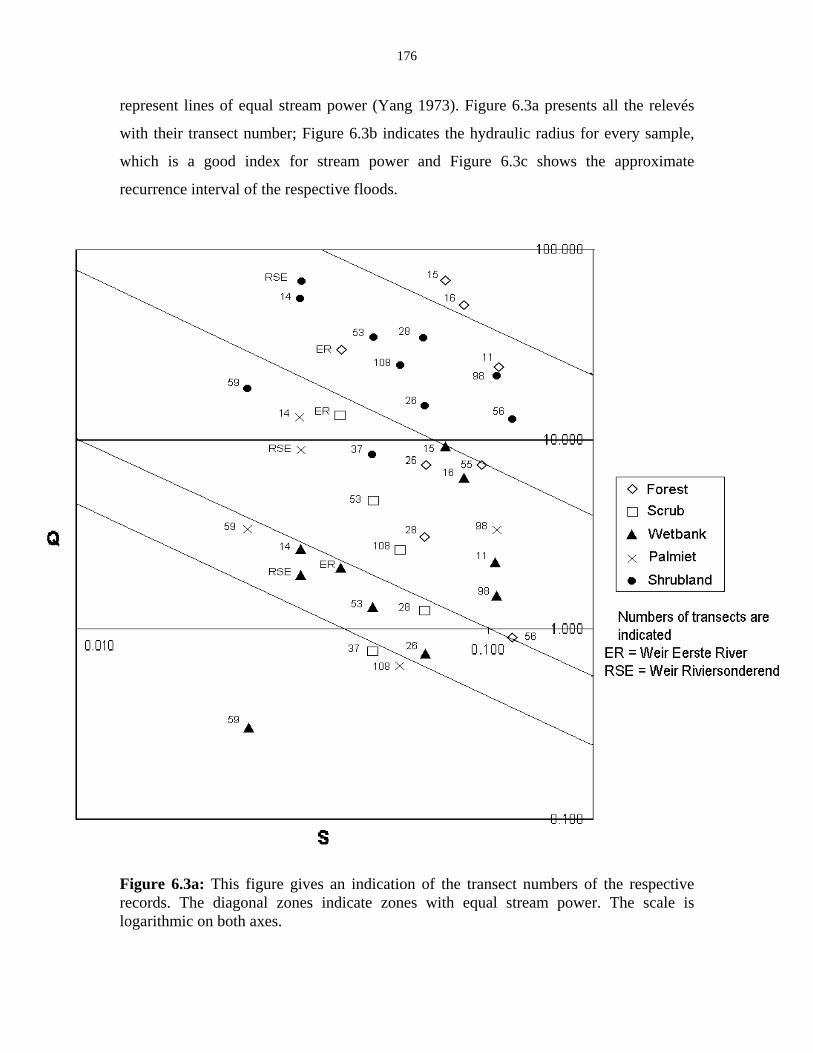
176
represent lines of equal stream power (Yang 1973). Figure 6.3a presents all the relevés
with their transect number; Figure 6.3b indicates the hydraulic radius for every sample,
which is a good index for stream power and Figure 6.3c shows the approximate
recurrence interval of the respective floods.
Figure 6.3a: This figure gives an indication of the transect numbers of the respective records. The diagonal zones indicate zones with equal stream power. The scale is logarithmic on both axes.
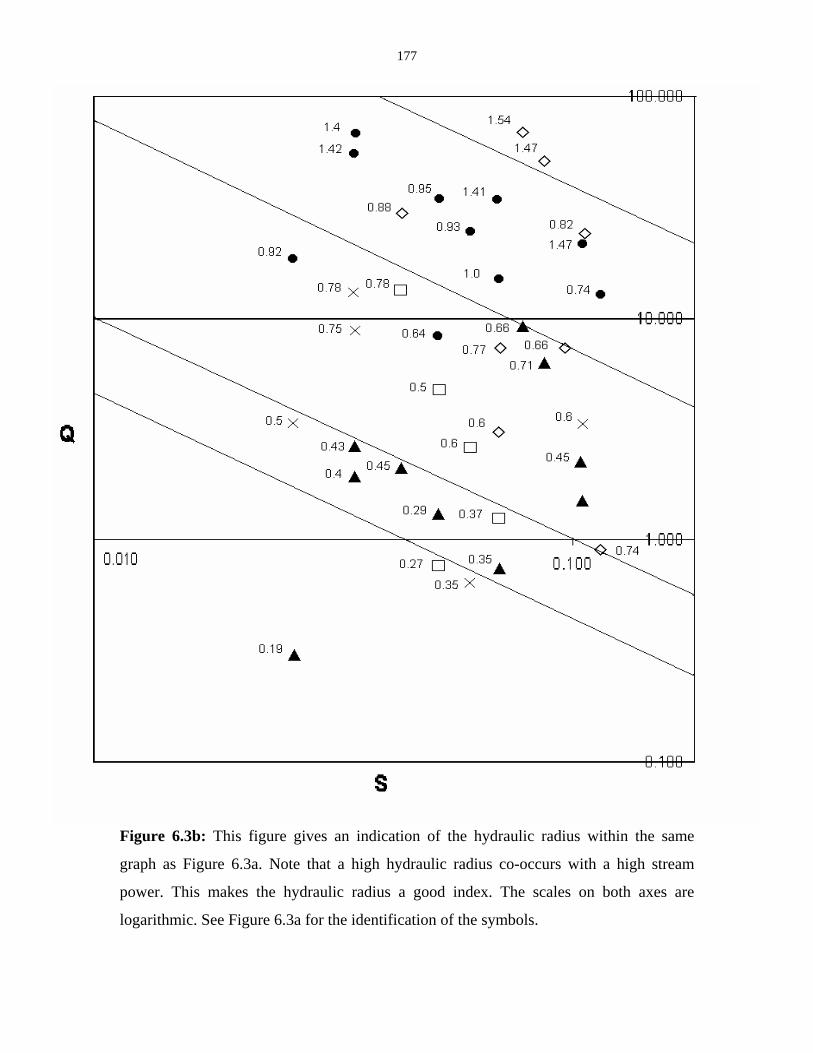
177
Figure 6.3b: This figure gives an indication of the hydraulic radius within the same
graph as Figure 6.3a. Note that a high hydraulic radius co-occurs with a high stream
power. This makes the hydraulic radius a good index. The scales on both axes are
logarithmic. See Figure 6.3a for the identification of the symbols.
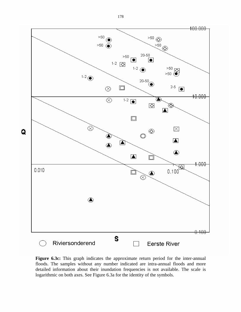
178
Figure 6.3c: This graph indicates the approximate return period for the inter-annual floods. The samples without any number indicated are intra-annual floods and more detailed information about their inundation frequencies is not available. The scale is logarithmic on both axes. See Figure 6.3a for the identity of the symbols.
179
At first sight these results might not seem very satisfactory. Most of the floods in
the graph are intra-annual floods for which the extrapolation method of Equation (6) does
not apply (Alexander 1991). The pattern of the interannual floods is confused. There is
no clear distinction in different bands between the one in two year floods and the one in
fifty year floods. The stream power, however, gives a much clearer picture. There are
well-defined bands for the Fynbos and for the Wet Bank vegetation while the Scrub Zone
and the Palmiet Zone occupy the same band. The only riparian zone that does not form a
clear band in the graph is Forest, which is found scattered over the entire graph. Note that
there are two outliers of Fynbos with lower stream power than the other samples of
Fynbos. Although the stream power is lower, the recurrence intervals of these two
samples are quite similar to those of other fynbos samples.
6.8 Discussion
Vegetation patterns
The vegetation patterns next to a river in the mountains are determined by two factors:
stream power and inundation frequency. It seems that the Wet Bank vegetation and the
Palmiet and Scrub Zone can be distinguished clearly from the stream power of the floods
running over them. Palmiet and Scrub do not occur together and seem to be
interchangable. The Palmiet Zone is mostly found in the Riviersonderend River and the
Scrub Zone mostly in the Eerste River. We assume that Scrub is mostly found in rivers
with steep banks where small floods coincide with large stream power, while Palmiet
thrives on the gentler banks where less damage is done to the vegetation during regular
floods.
Fynbos is found on the outer edges of the riparian zone and structurally it is
similar to the vegetation in the adjacent non-riparian uplands. The riparian fynbos types
are able to withstand high stream powers, but they are flooded only rarely. The
mechanical disturbance of the flood might well be so severe that a certain part of the
vegetation has to regenerate after a high flood, especially in cases of the one in fifty year
floods, where whole lifespans of fynbos plants take place in between floods. Riparian
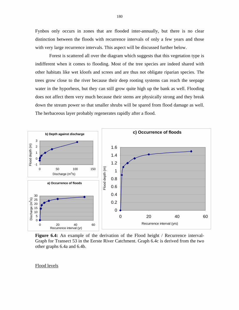
180
Fynbos only occurs in zones that are flooded inter-annually, but there is no clear
distinction between the floods with recurrence intervals of only a few years and those
with very large recurrence intervals. This aspect will be discussed further below.
Forest is scattered all over the diagram which suggests that this vegetation type is
indifferent when it comes to flooding. Most of the tree species are indeed shared with
other habitats like wet kloofs and screes and are thus not obligate riparian species. The
trees grow close to the river because their deep rooting systems can reach the seepage
water in the hyporheos, but they can still grow quite high up the bank as well. Flooding
does not affect them very much because their stems are physically strong and they break
down the stream power so that smaller shrubs will be spared from flood damage as well.
The herbaceous layer probably regenerates rapidly after a flood.
Figure 6.4: An example of the derivation of the Flood height / Recurrence interval-Graph for Transect 53 in the Eerste River Catchment. Graph 6.4c is derived from the two other graphs 6.4a and 6.4b. Flood levels
b) Depth against discharge
-1
0
1
2
3
0 50 100 150Discharge (m3/s)
Floo
d de
pth
(m)
a) Occurrence of floods
05
1015202530
0 20 40 60Recurrence interval (yr)
Dis
char
ge (m
3 /s)
c) Occurrence of floods
0
0.2
0.4
0.6
0.8
1
1.2
1.4
1.6
0 20 40 60Recurrence interval (yrs)
Floo
d de
pth
(m)
181
The main distinction between the floods is between the intra-annual and the inter-annual
floods. In Figures 6.3a to 6.3c the zones affected by the intra-annual floods are further
subdivided into zones affected by different stream power, but there is no clear
subdivision within the zones affected by inter-annual floods, or at least, that has not
become clear with the methods used in this study.
But the methodology need not be the limiting factor. Slight elevations in the water
level coincide with huge additional discharges, especially in the higher zones up the
banks. The difference in the discharges of the one in two year floods and the one in fifty
year floods is relatively small, so the difference in the water level will not be as
substantial as one would expect. Figure 6.4 illustrates an example of the Flood height /
Recurrence Interval-Graph derived from two discharge graphs. The example shows a
transect in the Eerste River. It is clear that the difference in water level is negligible in
the larger recurrence intervals. Since banks are often relatively steep, vegetation bands
reflecting, for example, a one in ten year flood would be very narrow, whereas in the
lower reaches these vegetation patterns would be clear because of the greater bank
widths. In the Riviersonderend the situation is even more extreme, because differences in
discharge are smaller here than in the Eerste River (see Table 6.1). This might be due to
the extrapolation using Equation 5, but it could also be that the Riviersonderend has a
different seasonal water regime.
Methods used
The methodology used in this study can be applied in general to mountain streams where
discharges measured at weirs need to be extrapolated further upstream. This is a positive
outcome, because the more precise measurement of discharges in mountain streams
would involve measurement of rainfall intensity, which is only very rarely available.
There are however a few critical factors in the equations that deserve some further
attention:
Slope: slope needs to be measured very precisely, because a slight difference in slope can
cause a huge difference in discharge. In this study two measurements of slope were used:
one was measured directly in the field with a slope meter and one was derived from
182
orthographic maps. The first measurement, which is the slope on a small scale, produced
the best results, which were used in the rest of the study. When slopes are too steep (>
10%) Equation (4) does not apply any more.
Boulder sizes: The roughness equations require the median and 84% percentile of the
boulder size. Equation (4) is quite sensitive to the values chosen for these percentiles so it
is important to make a good estimate. If there is a large spread in boulder size, in other
words, a large difference between d50 and d84, it results in large values for roughness and
lower discharges. In this respect the situation in the mountain streams in the Western
Cape often poses a problem, because there is indeed a large spread in boulder sizes.
There are mostly two size classes, a class of big rocks with a diameter of about 1 to 1.5
metres and a class of small boulders with a diameter of about 0.2 to 0.4 metres. The
calibration of Equation (4) in the literature (Simons & Senturk 1992) is derived from
situations where d50/d84 is on average 2.18 and maximally 6.0. The boulder sizes in this
study still fall within this range, but high values for d50/d84 often produce extremely high
values for Manning’s n. We suggest that it might be best to estimate d50 and d84
separately for each of the size classes. This will however require further investigation. In
this study only the small rocks have been used, but it would probably be prudent to
concentrate on the bigger rocks when calculating big floods and to use the smaller rocks
when calculating small floods. In a small flood, the big rocks do not have a large
influence on the roughness because they mainly stick out of the water, while in a large
flood the roughness is mainly determined by the large rocks and the influence of the
small ones is negligible.
6.9 Conclusion
The main questions concerning the hydraulics of rivers upstream from the highest weirs
are about understanding the natural ecosystem. The methods used in this study are
reasonably efficient in achieving this aim, and a correlation between the vegetation
zonation patterns and the hydraulics of the channel could be shown in graphs such as
Figure 6.3.

183
However, in comparison to the standards of accuracy attainable in the lower
reaches of the rivers, the methods used are not accurate at all and the calculated
recurrence intervals in particular might easily be out of range by more than 25%.
The only way to get more accurate data is to use weirs or other expensive
instruments in the highest reaches to collect exact measurements at several locations in a
mountain catchment. Since there is no direct need from society’s point of view, it is quite
unlikely that this will happen soon. In the meantime, the methodology described here
provides a cheap and reasonably efficient technique.
184
7. Scaling of environmental factors structuring riparian vegetation in
the species-rich Fynbos Biome
Keywords: Riparian vegetation, Fynbos Biome, Gradient analysis, Hierarchical scaling,
Canonical Correspondence Analysis, Variation Partitioning, South Africa.
Nomenclature: Goldblatt & Manning (2000)
7.1 Abstract
A combination of hierarchical scaling and variation partitioning is used to describe
patterns of riparian vegetation in mountain catchments in the Hottentots Holland
Mountains, Western Cape, South Africa. Three different gradients are defined in order to
describe the complex vegetation patterns found here. The geographical gradient describes
the climatic and topographical changes across the entire mountain range. The
longitudinal gradient describes the changes along the different river reaches. The lateral
gradient describes the processes along the profile of the riverbed. The three gradients
operate on three different hierarchical scales. Partial Canonical Correspondence Analysis
is used to determine the amount of variation that is explained on each of the hierarchical
scales. The geographical gradient accounts for the highest fraction (more than 50%) of
the TVE (total variation explained). This reflects the high gamma diversity in the Fynbos
Biome. The spatial variation that is not explained by the geographical gradient is a very
small fraction, which suggests that the variables used for description of the geographical
gradient are acceptable. The most important among these are geology and the fraction of
annual precipitation that falls in the driest months. The second most important gradient is
the lateral gradient, which reflects stream power and inundation frequencies of the river.
This gradient represents about one third of the explained variation. The longitudinal
gradient is the least important of the gradients and reflects considerable overlap with the
geographical gradient, because climatic changes also occur within the catchment. This
gradient mainly explains the amount of erosion or deposition that takes place in a
particular river reach. This is reflected best in the Wet Banks, the riparian zones that are
inundated on an annual basis.
185
Abbreviations used in this chapter: CCA = Canonical Correspondence Analysis, CA =
Correspondence Analysis, TVE = Total Variation Explained (by all explanatory
variables); TI = Total Inertia.
7.2 Introduction
Riverine ecosystems belong to the most complex ecosystems in the world. Day et al.
(1986) describe them as having four dimensions: the longitudinal axis of the river, the
profile of the riverbed, the elevation of the water level and the time-scale. The riparian
zones next to the river are very dynamic ecosystems, because they are subjected to both
the disturbances coming from the river and to those from the surrounding uplands, such
as fire, herbivory and disease. This creates a very heterogeneous environment where
many different species find their own niche (Gregory et al. 1991). Furthermore, the river
and the riparian zone reflect much of the environmental heterogeneity in the catchment,
because many of the nutrients occurring in the substrate of the catchment find their way
into the river (Rogers & Van der Zel 1989; Naiman & Décamps 1997) and the vegetation
in the riparian zone is dependent on the underlying substrate. From their side, riparian
habitats influence the instream biota by shading and nutrient inputs (King 1981; Stewart
& Davies 1990; Stewart 1992).
Rivers themselves also create heterogeneity on their banks, for example by
depositing sediment on the inner bend of a meander (Gregory et al. 1991). This makes
riparian ecosystems a good showcase for the hierarchical patch dynamics theory of Wu &
Loucks (1996). Van Coller et al. (2000) suggested, in their study of the Sabie River in
South Africa, that riparian ecosystems can best be studied by a combination of patch
dynamics and gradient analysis. The different scales at which environmental influences
operate on riparian vegetation are also shown by Jean & Bouchard (1993), Malanson
(1993), Ward & Wiens (2001) and Decocq (2002).
This study aims to propose a different view on riparian ecosystems by focusing on
the mountain streams in the Fynbos Biome in the Western Cape. Except for the habitat
diversity normally encountered in riparian habitats, this area has an extremely high
species diversity (Taylor 1978; Kruger & Taylor 1979; Cowling et al. 1992), due to a
complex evolutionary history (Goldblatt 1978; Linder et al. 1992) and to sharp ecological
186
gradients (Campbell 1983; Cowling et al. 1992; McDonald et al. 1996). The complex
vegetation patterns that are a result of these two superimposed ecosystems will be
revealed by an approach that theoretically resembles the hierarchical scaling used by Van
Coller et al. (2000) and methodologically makes use of variation partitioning described
by Borcard et al. (1992) and Økland & Eilertsen (1994).
The study area that is chosen to reveal these vegetation patterns is the Hottentots
Holland Mountain range in the southwestern Cape, South Africa.
7.3 Study area
The Hottentots Holland Mountains are situated between the towns of Stellenbosch,
Franschhoek and Grabouw in the Southwestern Cape. A map of the study area is
presented in Chapter 2, Figure 2.1. Five different rivers originate in this extremely wet
environment: the Berg River (a major river that flows north through the coastal forelands
to the Atlantic Ocean), the Riviersonderend River (another major river that flows east
through the Overberg Region to join the Breede River near Swellendam), the Palmiet
River (an intermediate sized river that flows south to the Atlantic Ocean), the Eerste
River (a small river that flows west through Stellenbosch towards the False Bay coast)
and the Lourens River (a small river that flows into False Bay near Somerset West).
Oliver et al. (1983) and Cowling et al. (1992) identify this area, together with the
Kogelberg located immediately south of the Hottentots Holland Mountains, as the core
area of the Fynbos Biome. The species and habitat diversity in this area are very high
(Campbell 1983; Deacon et al. 1992) which makes the area an attractive subject for
gradient analysis.
7.4 Climate
The Hottentots Holland Mountains enjoy a climate classified as Csb in the Köppen
(1931) system, which is a mediterranean climate with hot dry summers and mild wet
winters. The climate at high altitudes is slightly different from the climate in the valleys,
because rainfall increases and temperature decreases with altitude (Versfeld et al. 1992).
Sixty per cent of the precipitation falls in the wettest four months - from June to
September. This precipitation is mostly in the form of rain but snow can also occur on the
187
mountain peaks in winter (Fuggle & Ashton 1979). Schulze (1965) mentions a total
precipitation on the tops of the Hottentots Holland Mountains in excess of 3000 mm per
annum. The high precipitation in the mountains is caused by orographic rain precipitating
during both winter and summer months (Deacon et al. 1992). Rainfall patterns in the
mountains are extremely complex and the only detailed study in the area, so far, is by
Wicht et al. (1969). Solar radiation on the mountaintops is high, but temperatures drop
0.5° C for every 100 metres. Temperature records from the higher altitudes are sparse to
non-existent in many areas (Fuggle & Ashton 1979).
7.5 Geology and pedogenesis
Sandstones of the Table Mountain Group dominate the geology of the Hottentots Holland
Mountains. Within the sandstones there are two shale bands that can be accompanied by
tillite, one at high altitude and one at low altitude (De Villiers et al. 1964). On the
western slopes much older deposits of the Cape Granite Suite cover the valley bottoms,
most extensively in Jonkershoek, but also in Banghoek Kloof and at Lourensford. In
Assegaaibosch Kloof granite is also found at the edge of the Hottentots Holland Nature
Reserve. The Jonkershoek Valley has many faultlines along the axis of the valley. In a
small area on the southwestern slopes of Stellenbosch Mountain shales of the
Malmesbury Group are found (South African Committee for Stratigraphy 1980).
Most soils developing on quartzite are very shallow and poorly developed.
Podzolization is the most important soil-forming process (Fry 1987; Deacon et al. 1992).
Next to the river, soils are even more poorly developed because the finer particles and the
nutrients are washed away regularly. The substrates in riparian habitats mainly consist of
rocks but further away from the river deeper soils can be encountered. The soils under
riparian forest are mainly of the Magwa and the Oakleaf Forms, and on granites and
shales the Glenrosa Form can be encountered (Soil Classification Working Group 1991).
In mires at high altitudes the Champagne Form is most common while the Fernwood
Form is found on the edges of the mires (see Chapter 4).
188
7.6 Environmental gradients
Mountain streams have even higher habitat diversity than the lower reaches of these
rivers. Pools and riffles, cascades, waterfalls, large boulders and fallen logs all create a
complicated mosaic of different microhabitats. The patch hierarchy described by Van
Coller et al. (2000) for riparian ecosystems also applies to mountain streams, but because
the channels are in general much narrower, it is not a very suitable way to observe
mountain streams. Instead, longitudinal gradients are much steeper in mountain streams,
and consequently an approach of composite gradients was chosen.
Vegetation in the riparian zones in the study area is subject to very complex
environmental patterns, due to the many gradients that are found there. To unravel this
pattern we take a closer look at each of these gradients and the individual scales at which
each operates, separately. A direct gradient analysis is undertaken at each of these scales
(Whittaker 1967, 1973b). Therefore we start at the largest scale:
1. On the first hierarchical scale there is a climatic gradient across the mountains.
The Western Cape contains very sharp climatic gradients from the mesic climate on the
coast to the arid climate in the interior (Campbell 1983; Deacon et al. 1992). The amount
and the seasonality of the rainfall can change across a single mountain range. As a result,
gamma diversity is extremely high (Kruger & Taylor 1979; Cowling et al. 1992), even
for azonal vegetation types like riparian habitats (see Chapter 8). Each river catchment
experiences its own climatic regime. This gradient is referred to as the geographical
gradient and is described in detail by Campbell (1983), Deacon et al. (1992), Malanson
(1993) and McDonald et al. (1996). The gradient is very dependent on the topography
and on the locality of the sampling site. For this reason, Borcard et al. (1992) suggest that
all the geographical coordinates of each relevé and its quadratic and cubic products
should be recorded.
2. On the second hierarchical scale there is the gradient along the longitudinal
axis of the river. Here, not only the altitude changes, but also the nature of the river
reach. Altitude has a major impact on the climate and zonal vegetation also changes with
altitude (Campbell 1983). In general, rainfall is higher at high altitudes while
temperatures are lower. Because the gradient of the river decreases, river reaches at lower
altitudes have less erosive power than those at higher altitudes. This gradient is referred
189
to as the longitudinal gradient and is described by Vannote et al. (1980), Minshall et al.
(1983), Day et al. (1986), Fetherston et al. (1995) and Davies & Day (1998).
3. On the third hierarchical scale, a very clear gradient occurs across the riverbed,
representing zones of different inundation frequency. This gradient is most obvious in a
floodplain, as was described by Illichevsky (1933) for rivers in Eastern Europe. The
study by Glavaç et al. (1992) confirms that vegetation units are very conspicuous and
vegetation borders are generally very sharp in riparian zones. In a mountain stream the
vegetation zones are more compressed than in the lower reaches but differences in
vegetation are just as conspicuous. Close to the river, inundation frequency is high,
erosive power is large and stream power is low. Further away, inundation is less frequent,
deposition is more common and stream power can be very high. The gradient described
here is referred to as the lateral gradient and is described by Kopecky (1969), Menges &
Waller (1983), Hupp & Osterkamp (1985), Gregory et al. (1991), Glavaç et al. (1992),
Dixon & Johnson (1999), Boucher & Tlale (1999) and Bendix (1999).
Superimposed on these gradients are environmental characteristics of a ‘patchy’
nature. These operate mainly at a larger scale, like geology and soil types. These
variables are recorded as nominal variables. Some other soil variables, which are not
nominal, are dependent on the substrate and the climatic conditions and are also included
in the geographical gradient, like contents of organic material and pH.
This description clearly demonstrates that there are three hierarchical scales in
which an environmental gradient can be described. These gradients are referred to as
nested environmental gradients. In the study area, vegetation surveys have been done in
five different catchments, which are subject to a climatic gradient. Within each catchment
there is an altitudinal gradient and at every sample site there is a gradient in inundation
frequency. On top of these three ‘nested environmental gradients’ there are different
geological substrates that also have a profound influence on the riparian vegetation. A
schematic review of these three gradients is illustrated in Figure 7.1.
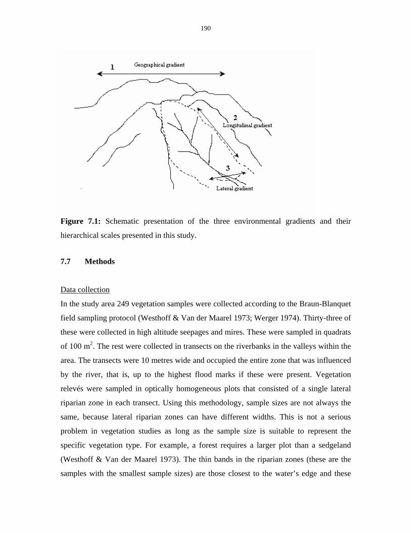
190
Figure 7.1: Schematic presentation of the three environmental gradients and their
hierarchical scales presented in this study.
7.7 Methods
Data collection
In the study area 249 vegetation samples were collected according to the Braun-Blanquet
field sampling protocol (Westhoff & Van der Maarel 1973; Werger 1974). Thirty-three of
these were collected in high altitude seepages and mires. These were sampled in quadrats
of 100 m2. The rest were collected in transects on the riverbanks in the valleys within the
area. The transects were 10 metres wide and occupied the entire zone that was influenced
by the river, that is, up to the highest flood marks if these were present. Vegetation
relevés were sampled in optically homogeneous plots that consisted of a single lateral
riparian zone in each transect. Using this methodology, sample sizes are not always the
same, because lateral riparian zones can have different widths. This is not a serious
problem in vegetation studies as long as the sample size is suitable to represent the
specific vegetation type. For example, a forest requires a larger plot than a sedgeland
(Westhoff & Van der Maarel 1973). The thin bands in the riparian zones (these are the
samples with the smallest sample sizes) are those closest to the water’s edge and these
191
mainly consist of sedge vegetation. They are sampled in areas of about 2 to 5 m2. The
vegetation further from the water’s edge consists of forest, scrub or fynbos and these are
sampled in areas of about 50 to 100 m2.
The vegetation types present in the plots are classified into 26 vegetation units at
the association-level (see Chapter 5).
Environmental variables describing the lateral, longitudinal and geographical
gradients have been determined for the majority of these relevés. The relevés from which
the environmental data is incomplete (mainly the aquatic vegetation) or that were
outliers, have been left out of further analysis, leaving a data set of 182 relevés with 182
species (the species with less than five occurrences were left out). In the majority of
analyses the seepages were left out because they were the cause of considerable
heterogeneity in the data set. This resulted in a data set of 150 relevés and 161 species. It
must be noted, however, that in the highest reaches of the rivers many vegetation
elements of the seepages occur in the riparian zone, making the distinction between the
two ecosystems somewhat fuzzy (see Chapter 4).
Environmental variables
The environmental variables recorded along each transect included slope, aspect, geology
and the gradient of the river reach at the site (coded as GRAD1, Tab. 1). Other variables
were recorded in every sample within each transect; these included rockiness and several
soil variables. Electrical resistance and pH were recorded for the soil samples and the
organic matter contents were determined using the Walkley-Black method (Walkley
1935). Particle size distribution was determined by sieving (sieve sizes 2 mm, 250 μm,
106 μm, 63 μm) to separate Coarse sand, Medium sand, Fine sand and Silt respectively.
Soil types were determined using the limited data that were available, namely soil depth,
texture, organic matter contents, pH, habitat and the colour of the topsoil. Soils were
compared with the soils found in Fry’s (1987) study of fynbos soils in Swartboschkloof,
Jonkershoek, and then soil types were attributed on the grounds of this comparison.
However, most riparian soils are very poorly developed because of the dynamic
environment near rivers: soils are often washed away during floods and it is mainly the
boulders that remain. Distance and elevation from the water’s edge were recorded for
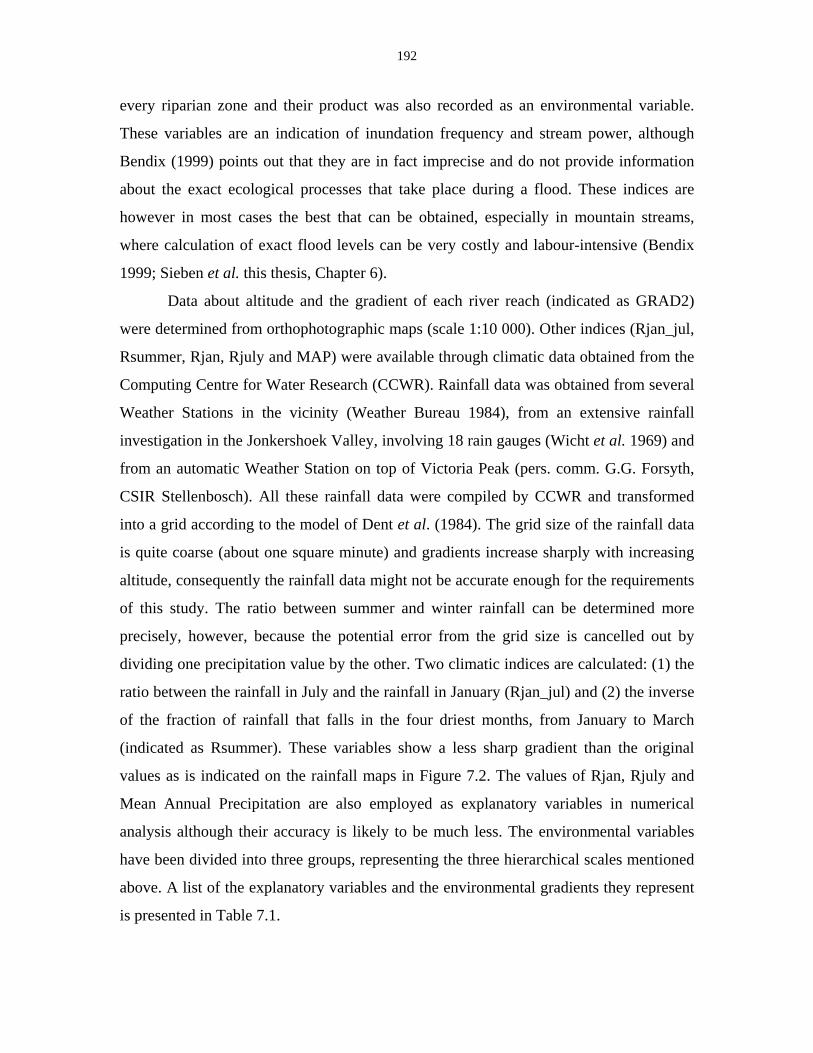
192
every riparian zone and their product was also recorded as an environmental variable.
These variables are an indication of inundation frequency and stream power, although
Bendix (1999) points out that they are in fact imprecise and do not provide information
about the exact ecological processes that take place during a flood. These indices are
however in most cases the best that can be obtained, especially in mountain streams,
where calculation of exact flood levels can be very costly and labour-intensive (Bendix
1999; Sieben et al. this thesis, Chapter 6).
Data about altitude and the gradient of each river reach (indicated as GRAD2)
were determined from orthophotographic maps (scale 1:10 000). Other indices (Rjan_jul,
Rsummer, Rjan, Rjuly and MAP) were available through climatic data obtained from the
Computing Centre for Water Research (CCWR). Rainfall data was obtained from several
Weather Stations in the vicinity (Weather Bureau 1984), from an extensive rainfall
investigation in the Jonkershoek Valley, involving 18 rain gauges (Wicht et al. 1969) and
from an automatic Weather Station on top of Victoria Peak (pers. comm. G.G. Forsyth,
CSIR Stellenbosch). All these rainfall data were compiled by CCWR and transformed
into a grid according to the model of Dent et al. (1984). The grid size of the rainfall data
is quite coarse (about one square minute) and gradients increase sharply with increasing
altitude, consequently the rainfall data might not be accurate enough for the requirements
of this study. The ratio between summer and winter rainfall can be determined more
precisely, however, because the potential error from the grid size is cancelled out by
dividing one precipitation value by the other. Two climatic indices are calculated: (1) the
ratio between the rainfall in July and the rainfall in January (Rjan_jul) and (2) the inverse
of the fraction of rainfall that falls in the four driest months, from January to March
(indicated as Rsummer). These variables show a less sharp gradient than the original
values as is indicated on the rainfall maps in Figure 7.2. The values of Rjan, Rjuly and
Mean Annual Precipitation are also employed as explanatory variables in numerical
analysis although their accuracy is likely to be much less. The environmental variables
have been divided into three groups, representing the three hierarchical scales mentioned
above. A list of the explanatory variables and the environmental gradients they represent
is presented in Table 7.1.
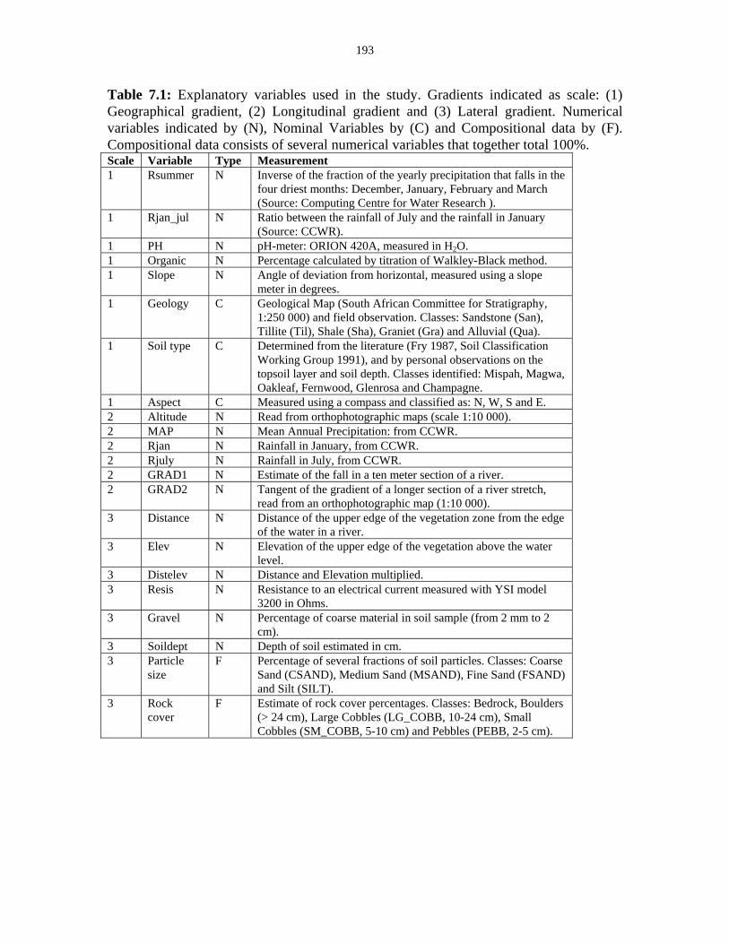
193
Table 7.1: Explanatory variables used in the study. Gradients indicated as scale: (1) Geographical gradient, (2) Longitudinal gradient and (3) Lateral gradient. Numerical variables indicated by (N), Nominal Variables by (C) and Compositional data by (F). Compositional data consists of several numerical variables that together total 100%. Scale Variable Type Measurement 1 Rsummer N Inverse of the fraction of the yearly precipitation that falls in the
four driest months: December, January, February and March (Source: Computing Centre for Water Research ).
1 Rjan_jul N Ratio between the rainfall of July and the rainfall in January (Source: CCWR).
1 PH N pH-meter: ORION 420A, measured in H2O. 1 Organic N Percentage calculated by titration of Walkley-Black method. 1 Slope N Angle of deviation from horizontal, measured using a slope
meter in degrees. 1 Geology C Geological Map (South African Committee for Stratigraphy,
1:250 000) and field observation. Classes: Sandstone (San), Tillite (Til), Shale (Sha), Graniet (Gra) and Alluvial (Qua).
1 Soil type C Determined from the literature (Fry 1987, Soil Classification Working Group 1991), and by personal observations on the topsoil layer and soil depth. Classes identified: Mispah, Magwa, Oakleaf, Fernwood, Glenrosa and Champagne.
1 Aspect C Measured using a compass and classified as: N, W, S and E. 2 Altitude N Read from orthophotographic maps (scale 1:10 000). 2 MAP N Mean Annual Precipitation: from CCWR. 2 Rjan N Rainfall in January, from CCWR. 2 Rjuly N Rainfall in July, from CCWR. 2 GRAD1 N Estimate of the fall in a ten meter section of a river. 2 GRAD2 N Tangent of the gradient of a longer section of a river stretch,
read from an orthophotographic map (1:10 000). 3 Distance N Distance of the upper edge of the vegetation zone from the edge
of the water in a river. 3 Elev N Elevation of the upper edge of the vegetation above the water
level. 3 Distelev N Distance and Elevation multiplied. 3 Resis N Resistance to an electrical current measured with YSI model
3200 in Ohms. 3 Gravel N Percentage of coarse material in soil sample (from 2 mm to 2
cm). 3 Soildept N Depth of soil estimated in cm. 3 Particle
size F Percentage of several fractions of soil particles. Classes: Coarse
Sand (CSAND), Medium Sand (MSAND), Fine Sand (FSAND) and Silt (SILT).
3 Rock cover
F Estimate of rock cover percentages. Classes: Bedrock, Boulders (> 24 cm), Large Cobbles (LG_COBB, 10-24 cm), Small Cobbles (SM_COBB, 5-10 cm) and Pebbles (PEBB, 2-5 cm).
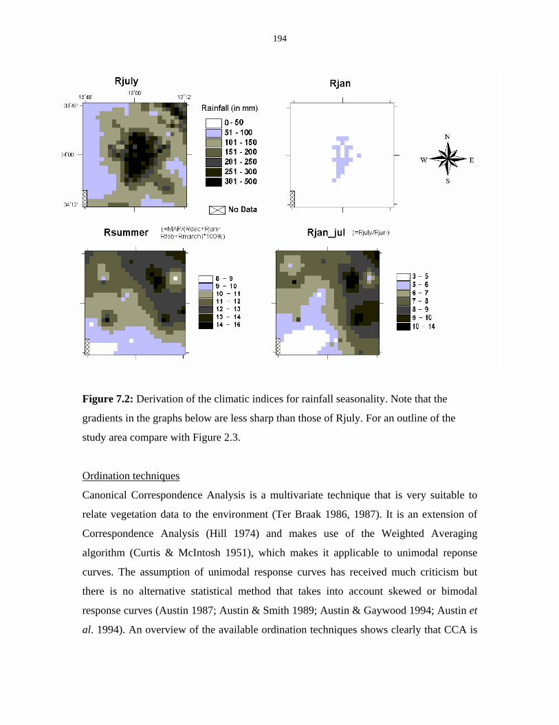
194
Figure 7.2: Derivation of the climatic indices for rainfall seasonality. Note that the
gradients in the graphs below are less sharp than those of Rjuly. For an outline of the
study area compare with Figure 2.3.
Ordination techniques
Canonical Correspondence Analysis is a multivariate technique that is very suitable to
relate vegetation data to the environment (Ter Braak 1986, 1987). It is an extension of
Correspondence Analysis (Hill 1974) and makes use of the Weighted Averaging
algorithm (Curtis & McIntosh 1951), which makes it applicable to unimodal reponse
curves. The assumption of unimodal response curves has received much criticism but
there is no alternative statistical method that takes into account skewed or bimodal
response curves (Austin 1987; Austin & Smith 1989; Austin & Gaywood 1994; Austin et
al. 1994). An overview of the available ordination techniques shows clearly that CCA is
195
the most suitable method for direct gradient analysis that is currently available (Jongman
et al. 1987; Legendre & Legendre 1999).
The Canonical Correspondence Analysis technique correlates the variation found
in the vegetation data to explanatory variables, which are supplied by the researcher. In
this way, it divides the variance into an explained and an unexplained part. The sum of all
the unconstrained eigenvalues, that is the result of a Correspondence Analysis, is a
measure of the total variation found in the data set and is referred to as the total inertia
(TI). The sum of the canonical eigenvalues (TVE) gives an indication of the fraction of
the variation that can be explained by the explanatory variables supplied (Økland 1994).
The unexplained part of the variation can be split into several portions, which are
clarified by Økland (1999). A part of it is ‘potentially explainable’, but for the greatest
part it consists of stochastic variation due to noise in the data set and to lack of fit to the
unimodal model. There is also a part of the unexplained variation that is due to the choice
of the explanatory variables. The best explanatory variables to use are those that quantify
directly the physiological processes that influence plant life, but these data are often very
difficult to obtain and so the methodology of data collection also has an impact on the
fraction of variation that is explained (Austin et al. 1984). To give an example relevant to
this study: if the inundation frequency of a river bank and the field capacity of the soils
are known, it would be a good quantification of the physiological stresses that riparian
plants experience, namely, anaerobic conditions in the root zone, followed by quicker or
slower drainage resulting in more arid conditions (Hewlett 1982). However, hydrological
data in the mountains is often lacking and it is impossible to collect undisturbed soil
samples from areas that are only accessible by foot. Explanatory variables that can be
used as an alternative are the distance from and the elevation to the water’s edge, and the
particle size distribution of the soils, which are easier to determine. These variables are
correlated to the ‘direct physiological’ variables, but are less accurate and will leave a
part of the variance unexplained.
In order to subdivide the explained variation further into several categories, Ter
Braak (1988) proposed an extension to CCA: Partial Canonical Correspondence
Analysis. With this method, the canonical axes of variance can be found after the
variance explained by certain variables (called covariables) has been removed. The
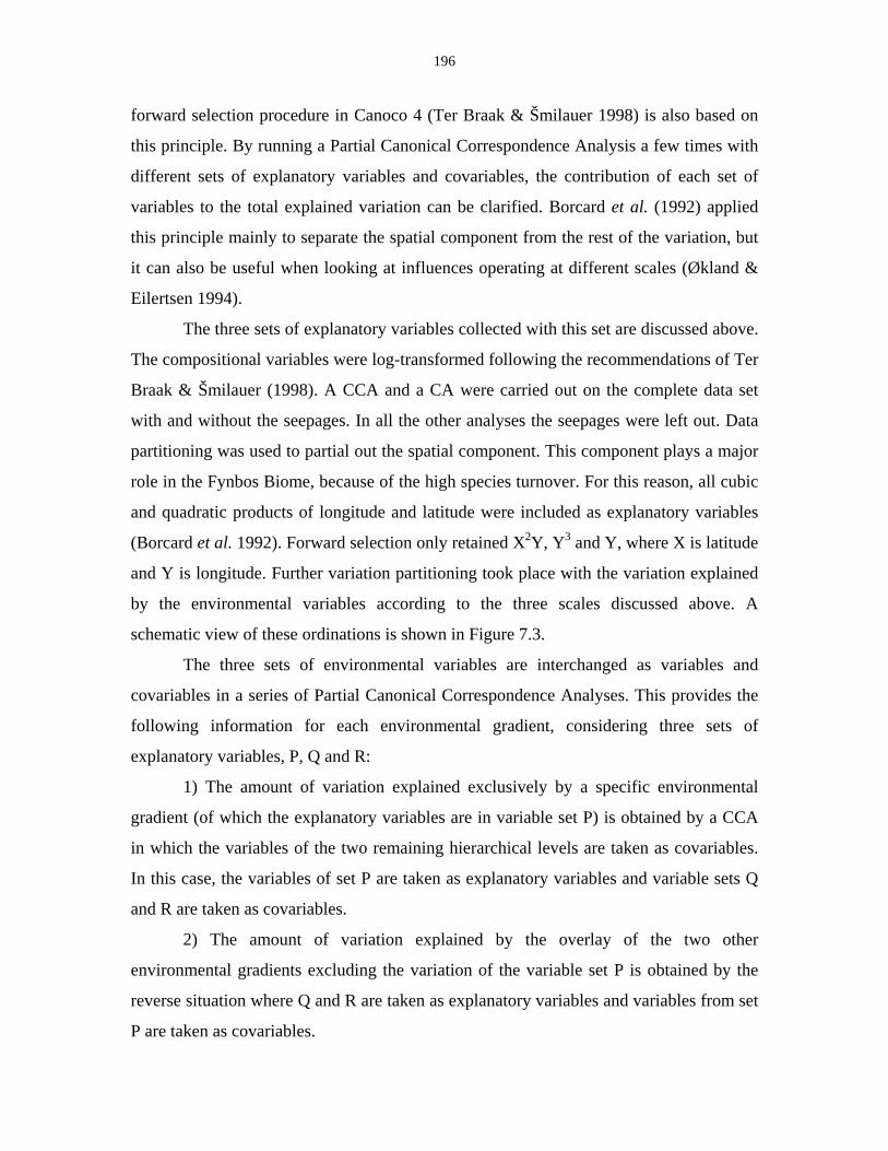
196
forward selection procedure in Canoco 4 (Ter Braak & Šmilauer 1998) is also based on
this principle. By running a Partial Canonical Correspondence Analysis a few times with
different sets of explanatory variables and covariables, the contribution of each set of
variables to the total explained variation can be clarified. Borcard et al. (1992) applied
this principle mainly to separate the spatial component from the rest of the variation, but
it can also be useful when looking at influences operating at different scales (Økland &
Eilertsen 1994).
The three sets of explanatory variables collected with this set are discussed above.
The compositional variables were log-transformed following the recommendations of Ter
Braak & Šmilauer (1998). A CCA and a CA were carried out on the complete data set
with and without the seepages. In all the other analyses the seepages were left out. Data
partitioning was used to partial out the spatial component. This component plays a major
role in the Fynbos Biome, because of the high species turnover. For this reason, all cubic
and quadratic products of longitude and latitude were included as explanatory variables
(Borcard et al. 1992). Forward selection only retained X2Y, Y3 and Y, where X is latitude
and Y is longitude. Further variation partitioning took place with the variation explained
by the environmental variables according to the three scales discussed above. A
schematic view of these ordinations is shown in Figure 7.3.
The three sets of environmental variables are interchanged as variables and
covariables in a series of Partial Canonical Correspondence Analyses. This provides the
following information for each environmental gradient, considering three sets of
explanatory variables, P, Q and R:
1) The amount of variation explained exclusively by a specific environmental
gradient (of which the explanatory variables are in variable set P) is obtained by a CCA
in which the variables of the two remaining hierarchical levels are taken as covariables.
In this case, the variables of set P are taken as explanatory variables and variable sets Q
and R are taken as covariables.
2) The amount of variation explained by the overlay of the two other
environmental gradients excluding the variation of the variable set P is obtained by the
reverse situation where Q and R are taken as explanatory variables and variables from set
P are taken as covariables.
197
Figure 7.3: Schedule with the ordinations done in this study to achieve variation
partitioning for three environmental gradients at three different scales.
In order to illustrate the variation on each hierarchical scale in detail, three other
Canonical Correspondence Analyses were carried out without variation partitioning
(These are not illustrated in Figure 7.3). They deal with one hierarchical scale at a time
and indicate which explanatory variables are most important at that specific scale. The
results of these ordinations are then illustrated in ordination diagrams showing the first
two canonical axes.
For the ordination of the first hierarchical scale (the geographic gradient), the
complete data set was used, but for the two other hierarchical scales the data set was split
into two. The actual purpose was to do the ordination on the second hierarchical scale
(the longitudinal gradient) within a single catchment, but then the data set would have to
be split into five, which would result in a very restricted data set. Instead, it was decided
to divide the data set into two groups of two similar catchments and to leave the fifth, the
Lourens River catchment out of further analyses, because of its aberrant vegetation types
(mainly Scree Forests, see Figure 7.5). After this split, the species occurring in less than
198
four relevés were left out. The Eerste and Berg Rivers are taken together to create a data
set of 74 relevés and 88 species. These catchments are similar in their total species
composition (see also Chapter 8), their geology (granite and shales in the valley bottoms
and sandstones at the higher altitudes), exposure (western and northern slopes) and
geomorphology (rivers originating on steep mountain headwalls). Data collected from the
Riviersonderend and Palmiet Rivers, combined together, result in a database of 91
relevés and 119 species. They can be grouped for the same reasons as the Eerste and Berg
Rivers, both being situated on the eastern and southern slopes, which are gentler and
underlain by sandstones and occasional shale bands. The resulting data sets are used for
Canonical Correspondence Analysis on the longitudinal and lateral gradients.
7.8 Results The classification of the vegetation samples resulted in 26 clusters of riparian vegetation
and nine clusters of seepages. These vegetation units are described in detail in Chapters 4
and 5. In order to illustrate these clusters in ordination diagrams the 26 original clusters
of riparian vegetation are combined to form 14 larger clusters, while the bogs and mire
types are regarded as one category. This subdivision is presented below together with the
most typical species that occur in them. The abbreviations of species used in the
ordination diagrams are indicated in brackets after the scientific names.
Wet Banks: These are the vegetation types found closest to the river’s edge. They
are subdivided into Pioneer Wet Banks (with mosses and juveniles of
trees and shrubs, forming Community Group 2), Erosion Wet Banks
(with species like Schizaea tenella (Schitene), Disa tripetaloides
(Disatrip), Drosera capensis (Droscape) and Prionium serratum
(Prioserr), forming Community Group 3) and Deposition Wet Banks
(with species like Juncus lomatophyllus (Juncloma) and Isolepis
prolifer, forming Community Group 4).
Ericaceous Fynbos: These are the most common fynbos types of the eastern slopes.
The most important species are Restio purpurascens (Restpurp), Erica
hispidula (Erichisp), Berzelia squarrosa (Berzsqua) and Leucadendron
199
xanthoconus. Five categories are recognized in the ordination diagrams.
The common type (Comm. 5.1 and 5.4) contains species like
Carpacoce spermacocea (Carpsper) and Restio burchelli. The high
altitude type (Comm. 5.3) also contains these species in combination
with Restio bifidus (Restbifi) and Tetraria crassa. A southern type
(Comm. 5.2) contains species like Tetraria capillacea (Tetrcapi) and
Erica intervallaris (Ericinte). There is one type (Comm. 5.5 and 6.1)
with seepage that is dominated by Cliffortia hirsuta (Clifhirs). The final
type (Comm. 6.2 and 6.3) is transitional to Asteraceous Fynbos and is
characterized by species like Muraltia heisteria and Stoebe cinerea.
Asteraceous Fynbos: These fynbos types are typical of the fine-grained soils on the
western slopes of the mountains. The most important species are
Myrsine africana (Myrsafri), Pteridium aquilinum (Pteraqui),
Helichrysum cymosum (Helicymo) and Cliffortia cuneata (Clifcune).
Three categories are recognized here. The common type (Comm. 7.1
and 7.2) contains the shrub Brabejum stellatifolium (Brabstel) and the
sedge Ficinia acuminata (Ficiacum). The type found on shale (Comm.
7.3) is characterized by Chasmanthe aethiopica (Chasaeth) and
Calopsis paniculata (Calopani). Then there is one type (Community
Group 8) that is dominated by Cliffortia odorata (Clifodor).
Forest and Scrub: These are the tallest non-fynbos riparian vegetation types. They are
subdivided into three categories. Afromontane Forest (Comm. 9.4)
contains species like Cunonia capensis (Cunocape), Maytenus
acuminata (Maytacum) and Todea barbara. Scree Forest (Comm. 9.2
and 9.3) contains these species together with Platylophus trifoliatus
(Plattrif) and Diospyros whyteana (Dioswhyt). Riparian Scrub
(Community Group 10) is very poor in species. The most important
species are Metrosideros angustifolia (Metrangu), Brachylaena
neriifolia (Bracneri) and Ischyrolepis subverticillata (Ischsubv).
Seepage Fynbos: Seepage Fynbos occurs at the sources of the rivers at high altitudes but
is left out of most analyses here because it is very different from the
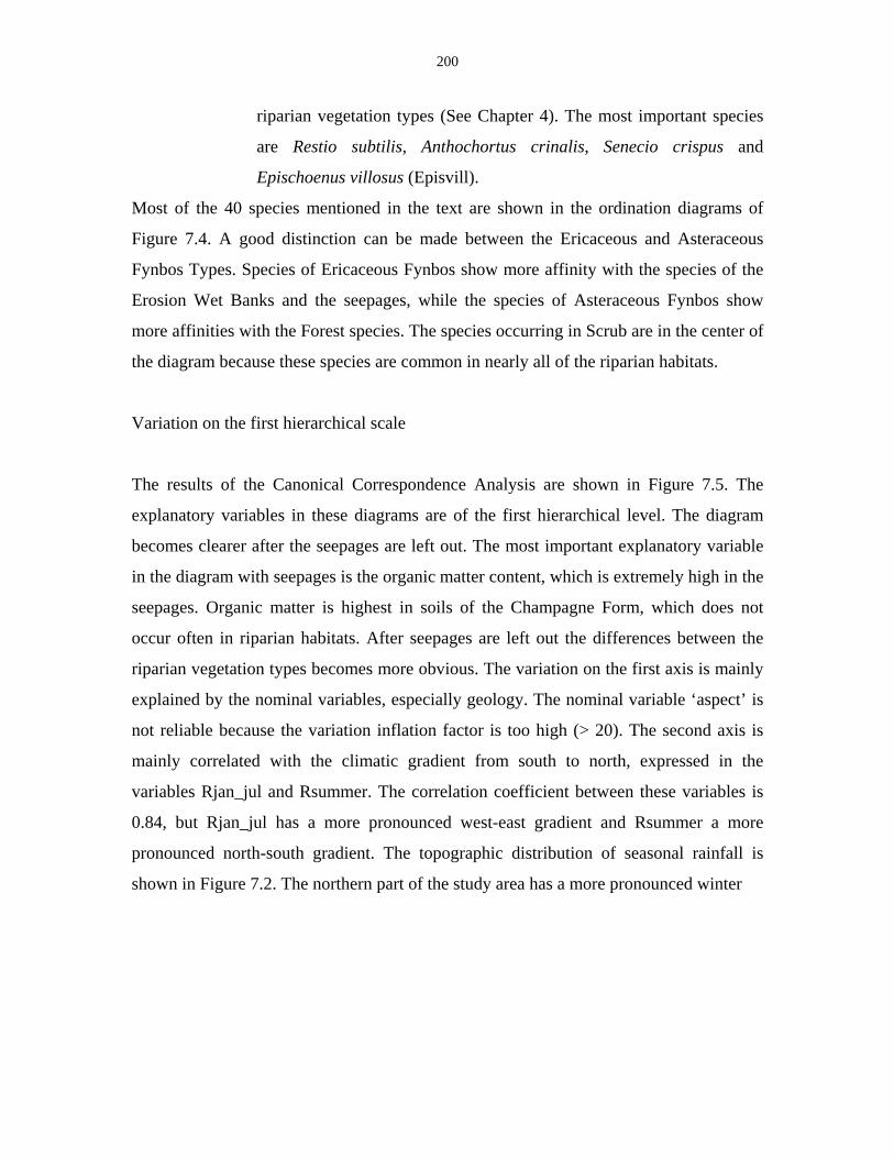
200
riparian vegetation types (See Chapter 4). The most important species
are Restio subtilis, Anthochortus crinalis, Senecio crispus and
Epischoenus villosus (Episvill).
Most of the 40 species mentioned in the text are shown in the ordination diagrams of
Figure 7.4. A good distinction can be made between the Ericaceous and Asteraceous
Fynbos Types. Species of Ericaceous Fynbos show more affinity with the species of the
Erosion Wet Banks and the seepages, while the species of Asteraceous Fynbos show
more affinities with the Forest species. The species occurring in Scrub are in the center of
the diagram because these species are common in nearly all of the riparian habitats.
Variation on the first hierarchical scale
The results of the Canonical Correspondence Analysis are shown in Figure 7.5. The
explanatory variables in these diagrams are of the first hierarchical level. The diagram
becomes clearer after the seepages are left out. The most important explanatory variable
in the diagram with seepages is the organic matter content, which is extremely high in the
seepages. Organic matter is highest in soils of the Champagne Form, which does not
occur often in riparian habitats. After seepages are left out the differences between the
riparian vegetation types becomes more obvious. The variation on the first axis is mainly
explained by the nominal variables, especially geology. The nominal variable ‘aspect’ is
not reliable because the variation inflation factor is too high (> 20). The second axis is
mainly correlated with the climatic gradient from south to north, expressed in the
variables Rjan_jul and Rsummer. The correlation coefficient between these variables is
0.84, but Rjan_jul has a more pronounced west-east gradient and Rsummer a more
pronounced north-south gradient. The topographic distribution of seasonal rainfall is
shown in Figure 7.2. The northern part of the study area has a more pronounced winter
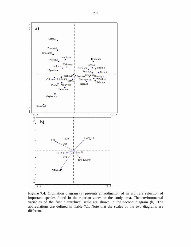
201
Figure 7.4: Ordination diagram (a) presents an ordination of an arbitrary selection of important species found in the riparian zones in the study area. The environmental variables of the first hierarchical scale are shown in the second diagram (b). The abbreviations are defined in Table 7.1. Note that the scales of the two diagrams are different.
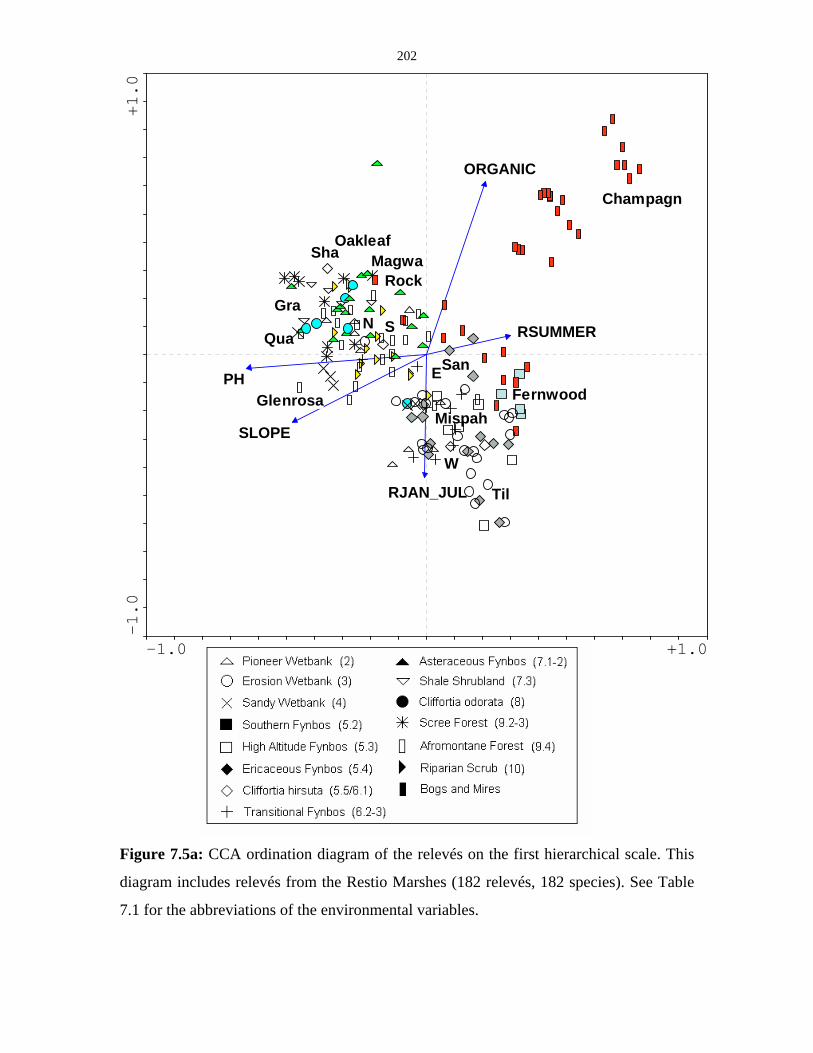
202
Figure 7.5a: CCA ordination diagram of the relevés on the first hierarchical scale. This
diagram includes relevés from the Restio Marshes (182 relevés, 182 species). See Table
7.1 for the abbreviations of the environmental variables.
-1.0 +1.0
-1
.0
+1
.0
PH
Champagn
SLOPE
GraRSUMMERQua
Sha
ORGANIC
Glenrosa Fernwood
Til
N
San
Rock
Oakleaf
S
W
Mispah
E
RJAN_JUL
Magwa
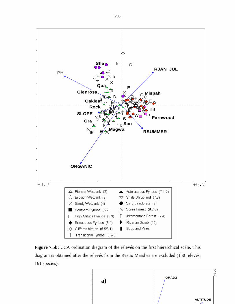
203
Figure 7.5b: CCA ordination diagram of the relevés on the first hierarchical scale. This
diagram is obtained after the relevés from the Restio Marshes are excluded (150 relevés,
161 species).
-0.7 +0.7
PH
ORGANIC
RJAN_JUL
SLOPETil
RSUMMER
Gra
Sha
Fernwood
Qua
W
Rock
Magwa
Mispah
Oakleaf
Glenrosa
San
N
S
E
ALTITUDE
GRAD2
+1.0
a)
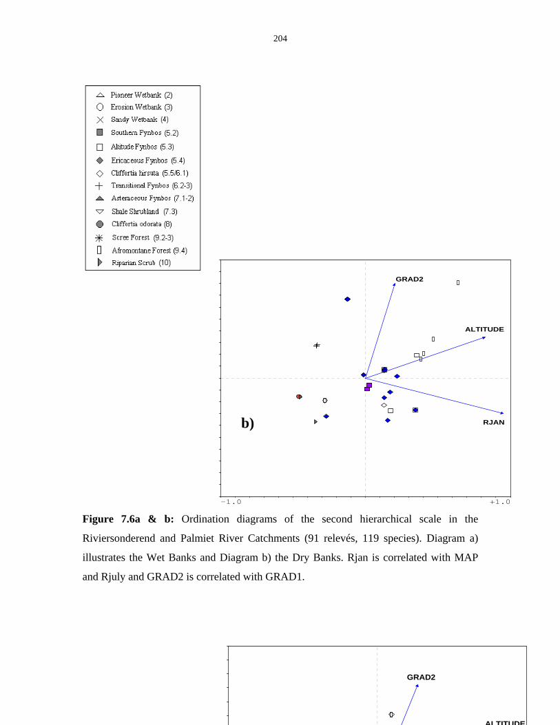
204
Figure 7.6a & b: Ordination diagrams of the second hierarchical scale in the
Riviersonderend and Palmiet River Catchments (91 relevés, 119 species). Diagram a)
illustrates the Wet Banks and Diagram b) the Dry Banks. Rjan is correlated with MAP
and Rjuly and GRAD2 is correlated with GRAD1.
-1.0 +1.0
RJAN
ALTITUDE
GRAD2
b)
ALTITUDE
GRAD2
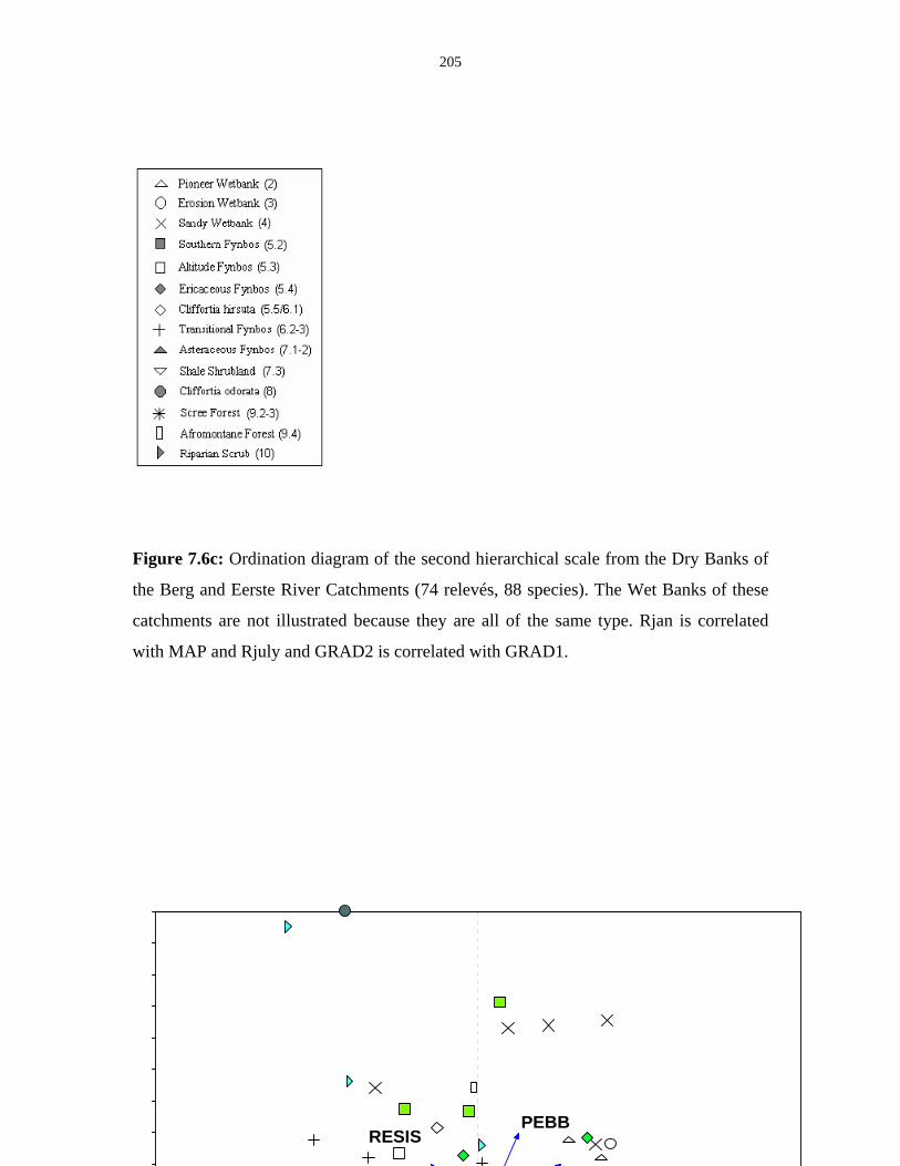
205
Figure 7.6c: Ordination diagram of the second hierarchical scale from the Dry Banks of
the Berg and Eerste River Catchments (74 relevés, 88 species). The Wet Banks of these
catchments are not illustrated because they are all of the same type. Rjan is correlated
with MAP and Rjuly and GRAD2 is correlated with GRAD1.
RESISPEBB
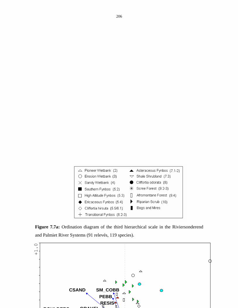
206
Figure 7.7a: Ordination diagram of the third hierarchical scale in the Riviersonderend
and Palmiet River Systems (91 relevés, 119 species).
+1
.0
BOULDERS
CSAND
GRAVELRESISPEBB
SM_COBB
207
Figure 7.7b: Ordination diagram of the third hierarchical scale in the Eerste and Berg
River Systems (74 relevés, 88 species).
rainfall aspect than the southern part. This means that water stress in summer is more
likely in the northern areas.
Variation on the second hierarchical scale
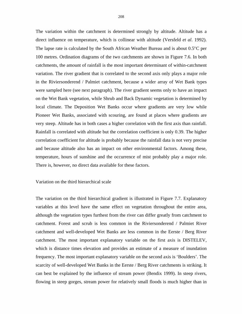
208
The variation within the catchment is determined strongly by altitude. Altitude has a
direct influence on temperature, which is collinear with altitude (Versfeld et al. 1992).
The lapse rate is calculated by the South African Weather Bureau and is about 0.5°C per
100 metres. Ordination diagrams of the two catchments are shown in Figure 7.6. In both
catchments, the amount of rainfall is the most important determinant of within-catchment
variation. The river gradient that is correlated to the second axis only plays a major role
in the Riviersonderend / Palmiet catchment, because a wider array of Wet Bank types
were sampled here (see next paragraph). The river gradient seems only to have an impact
on the Wet Bank vegetation, while Shrub and Back Dynamic vegetation is determined by
local climate. The Deposition Wet Banks occur where gradients are very low while
Pioneer Wet Banks, associated with scouring, are found at places where gradients are
very steep. Altitude has in both cases a higher correlation with the first axis than rainfall.
Rainfall is correlated with altitude but the correlation coefficient is only 0.39. The higher
correlation coefficient for altitude is probably because the rainfall data is not very precise
and because altitude also has an impact on other environmental factors. Among these,
temperature, hours of sunshine and the occurrence of mist probably play a major role.
There is, however, no direct data available for these factors.
Variation on the third hierarchical scale
The variation on the third hierarchical gradient is illustrated in Figure 7.7. Explanatory
variables at this level have the same effect on vegetation throughout the entire area,
although the vegetation types furthest from the river can differ greatly from catchment to
catchment. Forest and scrub is less common in the Riviersonderend / Palmiet River
catchment and well-developed Wet Banks are less common in the Eerste / Berg River
catchment. The most important explanatory variable on the first axis is DISTELEV,
which is distance times elevation and provides an estimate of a measure of inundation
frequency. The most important explanatory variable on the second axis is ‘Boulders’. The
scarcity of well-developed Wet Banks in the Eerste / Berg River catchments is striking. It
can best be explained by the influence of stream power (Bendix 1999). In steep rivers,
flowing in steep gorges, stream power for relatively small floods is much higher than in
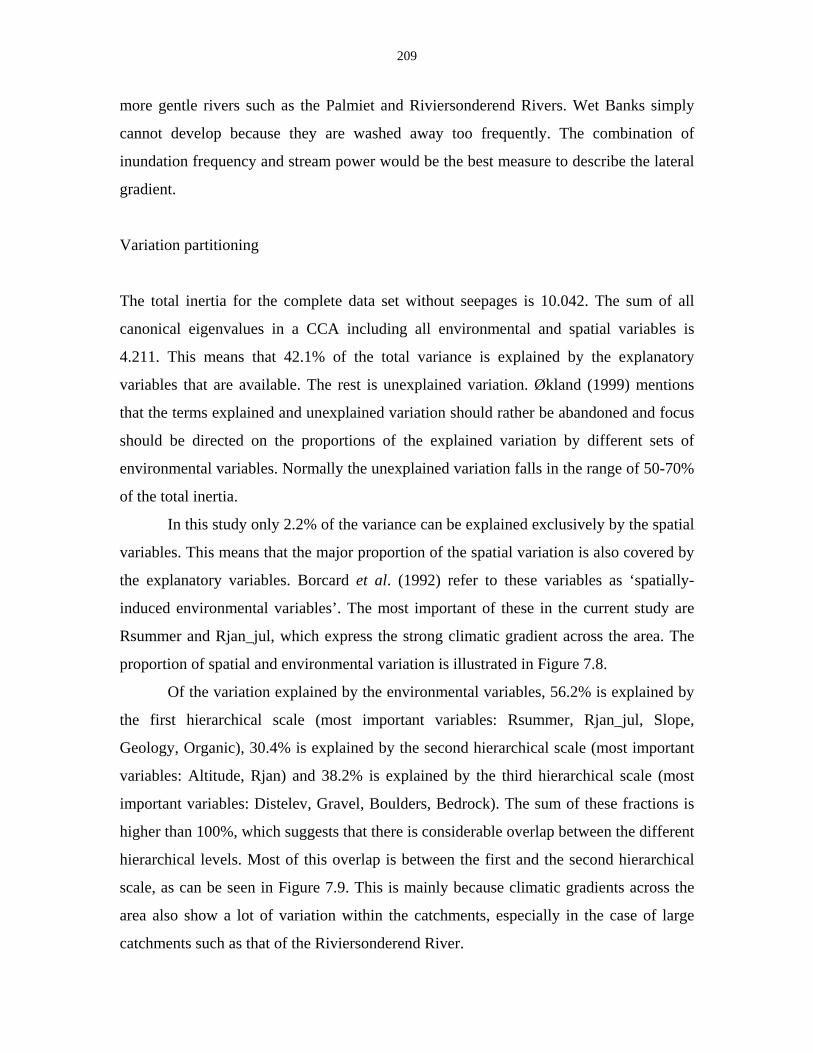
209
more gentle rivers such as the Palmiet and Riviersonderend Rivers. Wet Banks simply
cannot develop because they are washed away too frequently. The combination of
inundation frequency and stream power would be the best measure to describe the lateral
gradient.
Variation partitioning
The total inertia for the complete data set without seepages is 10.042. The sum of all
canonical eigenvalues in a CCA including all environmental and spatial variables is
4.211. This means that 42.1% of the total variance is explained by the explanatory
variables that are available. The rest is unexplained variation. Økland (1999) mentions
that the terms explained and unexplained variation should rather be abandoned and focus
should be directed on the proportions of the explained variation by different sets of
environmental variables. Normally the unexplained variation falls in the range of 50-70%
of the total inertia.
In this study only 2.2% of the variance can be explained exclusively by the spatial
variables. This means that the major proportion of the spatial variation is also covered by
the explanatory variables. Borcard et al. (1992) refer to these variables as ‘spatially-
induced environmental variables’. The most important of these in the current study are
Rsummer and Rjan_jul, which express the strong climatic gradient across the area. The
proportion of spatial and environmental variation is illustrated in Figure 7.8.
Of the variation explained by the environmental variables, 56.2% is explained by
the first hierarchical scale (most important variables: Rsummer, Rjan_jul, Slope,
Geology, Organic), 30.4% is explained by the second hierarchical scale (most important
variables: Altitude, Rjan) and 38.2% is explained by the third hierarchical scale (most
important variables: Distelev, Gravel, Boulders, Bedrock). The sum of these fractions is
higher than 100%, which suggests that there is considerable overlap between the different
hierarchical levels. Most of this overlap is between the first and the second hierarchical
scale, as can be seen in Figure 7.9. This is mainly because climatic gradients across the
area also show a lot of variation within the catchments, especially in the case of large
catchments such as that of the Riviersonderend River.
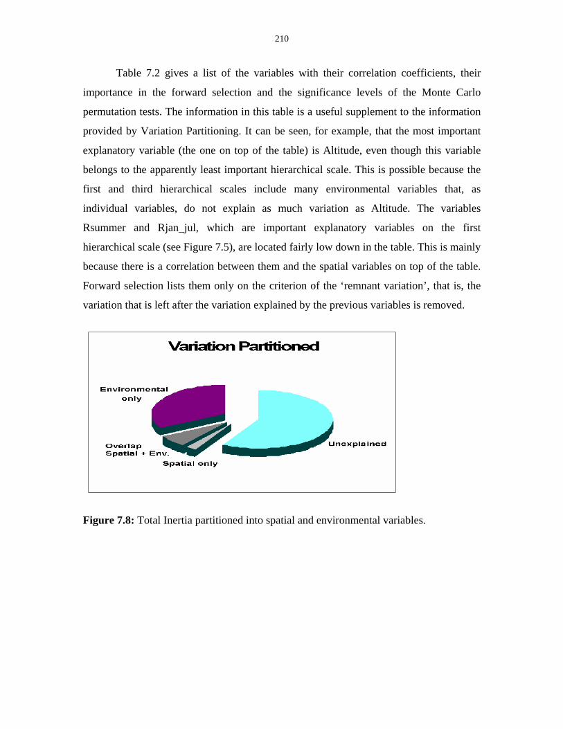
210
Table 7.2 gives a list of the variables with their correlation coefficients, their
importance in the forward selection and the significance levels of the Monte Carlo
permutation tests. The information in this table is a useful supplement to the information
provided by Variation Partitioning. It can be seen, for example, that the most important
explanatory variable (the one on top of the table) is Altitude, even though this variable
belongs to the apparently least important hierarchical scale. This is possible because the
first and third hierarchical scales include many environmental variables that, as
individual variables, do not explain as much variation as Altitude. The variables
Rsummer and Rjan_jul, which are important explanatory variables on the first
hierarchical scale (see Figure 7.5), are located fairly low down in the table. This is mainly
because there is a correlation between them and the spatial variables on top of the table.
Forward selection lists them only on the criterion of the ‘remnant variation’, that is, the
variation that is left after the variation explained by the previous variables is removed.
Figure 7.8: Total Inertia partitioned into spatial and environmental variables.
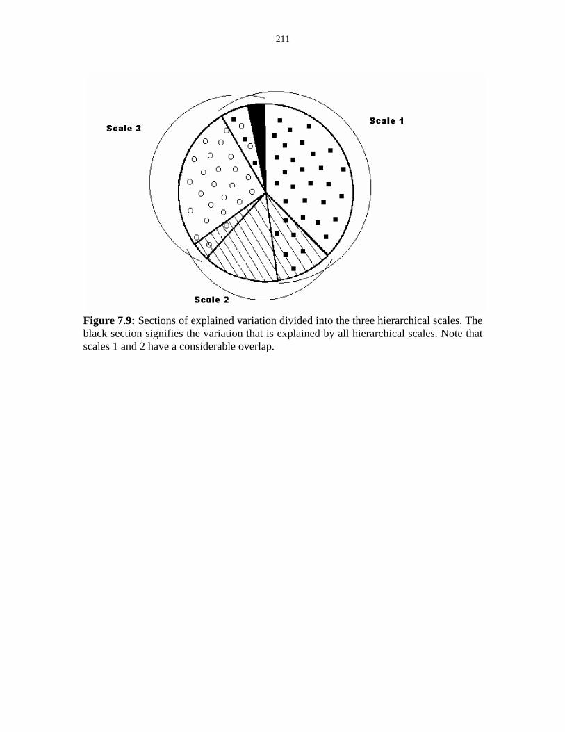
211
Figure 7.9: Sections of explained variation divided into the three hierarchical scales. The black section signifies the variation that is explained by all hierarchical scales. Note that scales 1 and 2 have a considerable overlap.
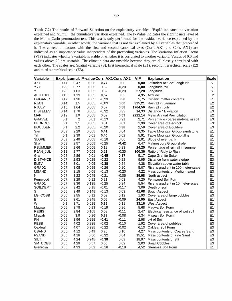
212
Table 7.2: The results of Forward Selection on the explanatory variables. ‘Expl.’ indicates the variation explained and ‘cumul.’ the cumulative variation explained. The P-Value indicates the significance level of the Monte Carlo permutation test. This test is only performed for the residual variance explained by the explanatory variable, in other words, the variance that is not yet explained by all variables that preceeded it. The correlation factors with the first and second canonical axes (Corr. AX1 and Corr. AX2) are indicated as an importance value independent of the preceeding variables. The Variation Inflation Factor (VIF) indicates whether a variable is stable or whether it is correlated to another variable. Values of 0.0 and values above 20 are unstable. The climatic data are unstable because they are all closely correlated with each other. The scales are: Spatial variable (S), first hierarchical scale (E1), second hierarchical scale (E2) and third hierarchical scale (E3).
Variable Expl. cumul. P-valueCorr. AX1Corr. AX2 VIF Explanation ScaleXXY 0,47 0,47 0,005 0,77 0,00 0,00 Latitude*Latitude*Longitude S YYY 0,29 0,77 0,005 0,32 -0,20 0,00 Longitude **3 S Y 0,26 1,03 0,005 0,32 -0,20 27,28 Longitude S ALTITUDE 0,16 1,19 0,005 0,57 0,33 4,95 Altitude E2 ORGANIC 0,17 1,36 0,005 -0,29 0,38 5,75 Organic matter contents E1 RJAN 0,14 1,5 0,005 -0,03 0,60 325,21 Rainfall in January E2 RJULY 0,15 1,64 0,005 0,07 0,58 1764,50 Rainfall in July E2 DISTELEV 0,14 1,78 0,005 -0,32 0,33 14,33 Distance * Elevation E3 MAP 0,12 1,9 0,005 0,02 0,59 2221,14 Mean Annual Precipitation E2 GRAVEL 0,1 2 0,01 -0,13 0,21 2,71 Percentage coarse material in soil E3 BEDROCK 0,1 2,1 0,005 0,01 0,01 1,99 Cover area of Bedrock E3 BOULDER 0,1 2,2 0,005 -0,20 0,38 2,58 Cover area of Boulders E3 San 0,09 2,29 0,005 0,41 0,04 9,35 Table Mountain Group sandstone E1 Til 0,1 2,39 0,01 0,40 0,02 5,91 Table Mountain Group tillite E1 SLOPE 0,09 2,48 0,005 -0,18 0,06 2,81 Slope of river bank E1 Sha 0,09 2,57 0,005 -0,25 -0,42 6,47 Malmesbury Group shale E1 RSUMMER 0,09 2,66 0,005 0,19 0,23 24,25 Percentage of rainfall in summer E1 RJAN_JUL 0,11 2,77 0,005 0,21 -0,30 100,36 Ratio of Rjuly to Rjan E1 Gra 0,08 2,86 0,01 -0,45 0,37 5,17 Cape Granite Suite E1 DISTANCE 0,07 2,93 0,025 -0,22 0,22 9,95 Distance from water's edge E3 ELEV 0,08 3,01 0,05 -0,38 0,24 4,38 Elevation above water table E3 GRAD2 0,07 3,08 0,065 -0,26 0,20 5,07 River's gradient in 100 meter-scale E2 MSAND 0,07 3,15 0,05 -0,13 -0,20 4,22 Mass contents of Medium sand E3 N 0,07 3,22 0,045 -0,21 -0,05 39,98 North aspect E1 Fernwood 0,07 3,29 0,12 0,21 0,03 4,20 Fernwood Soil Form E1 GRAD1 0,07 3,36 0,135 -0,25 0,24 5,54 River's gradient in 10 meter-scale E2 SOILDEPT 0,07 3,42 0,15 -0,01 -0,17 3,06 Depth of soil E3 S 0,06 3,49 0,145 -0,13 0,03 41,08 South Aspect E1 LG_COBB 0,06 3,55 0,12 0,02 0,12 1,93 Cover area of large cobbles E3 E 0,06 3,61 0,245 0,05 -0,09 24,95 East Aspect E1 W 0,1 3,71 0,015 0,35 0,11 33,16 West Aspect E1 Magwa 0,06 3,78 0,13 -0,19 0,26 5,68 Magwa Soil Form E1 RESIS 0,06 3,84 0,165 0,09 -0,11 2,47 Electrical resistance of wet soil E3 Mispah 0,06 3,9 0,26 0,38 -0,08 6,34 Mispah Soil Form E1 PH 0,06 3,96 0,255 -0,41 -0,11 2,98 pH of Soil E1 PEBB 0,06 4,02 0,285 -0,02 -0,10 1,92 Cover area of pebbles E3 Oakleaf 0,06 4,07 0,385 -0,22 -0,02 6,13 Oakleaf Soil Form E3 CSAND 0,05 4,12 0,49 0,25 0,10 4,27 Mass contents of Coarse Sand E3 FSAND 0,05 4,18 0,56 -0,32 0,04 15,51 Mass contents of Fine Sand E3 SILT 0,06 4,24 0,245 -0,38 0,09 18,97 Mass contents of Silt E3 SM_COBB 0,05 4,29 0,57 0,06 0,02 2,03 Small Cobbles E3 Glenrosa 0,05 4,33 0,63 -0,18 -0,18 4,52 Glenrosa Soil Form E1
213
7.9 Discussion The geographical gradient operating at the first hierarchical scale explains most variation
and is the most important gradient in this study. This is probably because of the
extremely high species turnover in the Fynbos Biome. The results of this study show
clearly that this even accounts for azonal vegetation like riparian vegetation. This is also
confirmed by A.B. Low, who compared river floras across the region, and found
significant differences between those floras. Although many riparian species have a wide
distribution and occur in many catchments, the total species composition of a specific
river is often very different from the river next to it (pers. comm. A.B. Low). As the
results of this study suggest, this can be mostly explained by differences in climate
regime and geology but also the river itself will probably play a role: the seeds of some
species are dispersed by water and for those species it will be easy to be dispersed
downstream in the same catchment, while it will be difficult to cross inhospitable habitats
to access another catchment. All in all, the geographical variation within the riparian
vegetation in the Fynbos Biome stands out. In other biomes and in areas with less strong
climatic gradients, the proportion of the variation explained by the geographical gradient
would probably be much less. This study only investigates a relatively small area, so it
would still be interesting to obtain data from other catchments throughout the Western
Cape to get a total picture. The importance of the geographical gradient in a river
ecosystem is also discussed by Malanson (1993).
The comparison of local floras is not the same as the comparison of diversity in
vegetation types but it does give an indication of what one can expect. Cowling &
Holmes (1992) give an indication of gamma diversity of non-riparian vegetation by
comparing six local floras throughout the Fynbos Biome. They clearly show that the
Southwestern part of the biome is the most diverse in species. It is likely that the
variation in (riparian) vegetation would show a similar picture, but this is not necessarily
so.
The lateral gradient is the next most important gradient. This gradient has been
studied in many vegetation studies before (Kopecky 1969; Hupp & Osterkamp 1985;
Glavaç et al. 1992; Boucher & Tlale 1999) and accounts for a high proportion of the
214
variation because the environmental stresses next to a river are very specific (Gregory et
al. 1991; Bendix 1999). It seems, however, that this variation is more obvious in the
lower reaches of the rivers, where riparian zones are more clearly developed. In the
highest reaches the riparian zones are often so much intertwined that they cannot be
distinguished from each other. Also, discharges are often not very high in these reaches,
so that different flood levels do not result in broad vegetation zones. Mountain streams
return to base levels more rapidly than rivers on the flats, hence inundation periods are
less determinative on the vegetation.
The longitudinal gradient, operating at the second hierarchical scale, is the least
important and shows a large overlap with the geographical gradient, because, within a
catchment, the variation in climate can still be quite large. The longitudinal gradient itself
has a small influence. The reach differences within the mountains do not have a direct
influence on the vegetation. The only aspect that is important about the reach is the
degree of erosion and deposition and this influence is best visible in the vegetation zones
closest to the river. It should be noted, however, that, within this study, only limited
stretches of river have been studied and that if rivers would be studied in their entirety,
including the lower reaches, the longitudinal gradient would play a major role, especially
since, in the Western Cape, the geology often changes to shales and calcareous sands in
the lower reaches of the rivers.
The type of analysis that was done in this study is a good way to get a total
overview of the river ecosystem and to map complex gradients across the landscape. To
recognize the three different scales in this study is important for the management of a
river ecosystem (Ward & Wiens 2001). Disturbances can affect either of the nested
gradients, for example channelization and alien shrubs affect the lateral gradient, and
dams and weirs affect the longitudinal gradient. The geographical gradient can be
distorted by climate change, but there is very little an individual manager can do about
this. The nested gradient approach is also a good way to model the original vegetation in
case of river rehabilitation after removal of severe infestations of aliens.
Except for a slight overlap between the longitudinal and geographical gradients,
there is very little overlap in the explained variation of each of the three gradients. This
demonstrates that the nested gradient approach is valid and that Variation Partitioning is
215
a good method to describe it. Variation partitioning possibly also minimizes the ‘arch
effect’ that occurs in CCA ordination diagrams, because this artefact is mainly caused by
hierarchical complexity (Allen 1987).
The weakness of the method is that the different variables operating at the
different scales have to be defined prior to the analysis. In general this is easy, but for
some variables the relation to the spatial scale is unclear or they operate at different
scales. For example, organic matter content is influenced by climate, so it operates at the
level of the geographical gradient. On the other hand, the river washes organic matter out
of the soil, so the lateral gradient also has an impact. In these cases it is best to choose the
largest scale. The results of this study show that these variables, in general, do not
explain a large part of the variation, with the notable exception of organic matter. This
will also reflect in the overlap between different scales as illustrated in Figure 7.9.
The approach used in this study is in sharp contrast to that by Van Coller et al.
(2000) who defined more nominal ‘patchy’ variables in riparian vegetation and set up a
hierarchy of these nominal variables. This main difference lies in the simple fact that Van
Coller et al. (2000) studied the lower reaches of the Sabie River, while this study aims at
describing the mountain stream habitat. The morphological units as they are defined by
Van Coller et al. (2000) are present in mountain streams but on a much smaller scale and
are mostly not vegetated at all, because of the poor substrate. The gradients are however
much sharper so the ‘nested gradient’ approach is more suitable for mountain streams,
while the ‘nested patches’ approach is more suitable for the lower reaches. But in this
case it is still possible to apply Variation Partitioning to lower river vegetation.
The methodology applied in Van Coller et al. (2000) and in this study revolves
around an old question in vegetation science: Is it scientifically allowable to have
preconceived ideas in order to describe the vegetation? In vegetation classification one is
allowed to undertake a reconnaisance survey prior to the actual fieldwork, and broad
vegetation and habitat units can be defined beforehand. This broad classification assists
in the assessment of the number of samples to be done and it can offer useful guidelines
for the final classification (Werger 1974; Westhoff & Van der Maarel 1973). The
assumption of random sampling promoted mainly by followers of the American tradition
has long been rejected (Whittaker 1973a; Shimwell 1971; Mueller-Dombois & Ellenberg
216
1974). This principle can be applied to gradient analysis as well. Just as it is useful for
classification to make an assessment beforehand, it will offer gradient analysis useful
guidelines if the existence of certain gradients is acknowledged beforehand, especially in
cases where it is already obvious that there is a pattern of nested gradients. ‘Random
gradient analysis’ would be an impossible prerequisite because the selection of
environmental variables already shows that the researcher has preconceived assumptions.
It should not be forgotten that gradient analysis is only a descriptive scientific method
and that causal relationships should not be derived from this method anyway.
7.10 Conclusions
A combination of hierarchical scaling and variation partitioning according to these scales
is a suitable method to describe a complex ecosystem with nested gradients. Riverine
ecosystems fall into this category, especially in the mountain reaches where there are
steep ecological gradients. In the lower reaches the geographical and longitudinal
gradients are in general less steep, except in the case of very large stretches of river. To
describe the more complex lateral gradients in the lower reaches the method of
hierarchical patch dynamics is very suitable.
Within an entire river ecosystem, gradient analysis would be possible when
combining the mountain reaches and the lower reaches. There will, however, be several
systems within the riverine ecosystem that are physically connected to the river but are
distinct systems of their own. The stagnant water conditions in the mires at the sources of
rivers and the saline conditions in the estuaries makes these parts of the river somewhat
different from the rest of the system and they should be studied separately. It would be
interesting to apply the nested gradient approach also to other river systems, different
reaches, larger stretches etc., so that general hypotheses about river ecosystems can be
derived from the results of these studies.
This study shows clearly that gradients in the Fynbos Biome are very sharp and
that this even reflects in the azonal vegetation types like the rivers. It is clear that azonal
vegetation is not only determined by small-scale ‘azonal’ processes, but is also an
expression of the large-scale climatic processes. Small fluctuations in climate, and the
217
anticipated global warming, will have a profound effect on this vegetation, because the
vegetation is very sensitive to the seasonal variation and amount of rainfall. In many
cases, large-scale processes also have their influence on small-scale processes, for
example rainfall determines the flow regime of the rivers (Hewlett 1982).
In the Fynbos Biome, not all riparian habitats are similar and to conserve the
maximal diversity in riparian habitats as many rivers as possible should be included in
conservation. In order to obtain this maximal variation, the three nested gradients in this
study and the most important explanatory variables can be used as guidelines. Most
mountain stream habitats are well conserved in South Africa because they are situated in
mountain catchments and they fall under the Water Conservation Act. Conservation
practices consist mainly of maintaining a natural flow regime and removing alien
vegetation. But perhaps the most important factor is that the prevailing climate in an area
remains unchanged. Global warming is an important threat to the Fynbos Biome and it
should be monitored to determine the extent in which the climate in these particular
catchments is affected by it. The wet habitats of the region will be the first ones to suffer
from changes in climate. This study should be followed by others in the biome in order to
monitor the effects of climate changes on the wet habitats of the biome.
218
8. Gamma diversity in an azonal vegetation type in the Fynbos Biome of
South Africa
Keywords: Gamma diversity, Fynbos Biome, riparian vegetation, similarity indices,
mountain catchment.
Nomenclature: Goldblatt & Manning (2000)
8.1 Abstract Similarity indices are used to examine the gamma diversity relationships in the riparian
floras of different catchment areas in the Hottentots Holland Mountain range in the
Fynbos Biome. The catchments are all part of the same mountain range. Two similarity
indices are used: the Jaccard Similarity Index and the Russell-Rao Similarity Index.
Comparisons are made between the catchments, the different altitudinal zones and the
different habitat types. Similarities are quite low, mainly because of the many rare
species. The most common species have a wide distributional range, but there are some
exceptions. There are only five species that were found in all the catchments, in all
altitudinal zones and in all habitat types. The riparian vegetation, like the other vegetation
types in the Fynbos Biome, has a high gamma diversity.
8.2 Introduction The Fynbos Biome is known as one of the most species-rich floras in the world
(Takhtajan 1969; Good 1974). The alpha and beta diversities are comparable to other
mediterranean-type climates, but it is the gamma diversity that stands out particularly
(Cowling et al. 1992). Kruger & Taylor (1979) mention areas that are only 25 km apart
and show a species turnover of more than 50%. This species diversity in the Fynbos
Biome can be explained partially by the origins of the fynbos species (Taylor 1978) but
also by the extreme radiation that took place in the wide array of environmental
conditions that can be found in the Western Cape (Campbell 1983; Deacon et al. 1992).
Climatic gradients are quite strong and the amount of precipitation at the higher altitudes

219
is many times that of the valleys (Wicht et al. 1969; Deacon et al. 1992). The species
radiation has occurred more strongly in certain taxonomic groups than in others and the
typical ‘fynbos taxa’ like Ericaceae, Restionaceae and Proteaceae have an extremely high
turnover of species, while cosmopolitan families like Poaceae and Orchidaceae are
under-represented when it comes to endemic species (Cowling et al. 1992).
Azonal vegetation, such as riparian vegetation, is rich in typical fynbos elements,
but it is mostly not as species-rich as the vegetation in the uplands (Kruger 1978b; Taylor
1978). In this respect, the situation in the Cape is quite different from Australia (Hancock
et al. 1996) or North America (Gregory et al. 1991). This situation is mostly due to the
huge species richness of the fynbos itself. The question addressed here is whether the
riparian vegetation elements reflect gamma diversity to the same degree as the adjacent
fynbos. For this purpose a comparison is made between the riparian vegetation of five
different catchments in the Hottentots Holland Mountains in the southwestern Cape (see
Figure 2.1).
8.3 Study area
The five catchments that were chosen for this study are all situated in the Hottentots
Holland Mountains. This Mountain Range is situated between the towns of Stellenbosch,
Franschhoek, Somerset West and Grabouw. It receives the highest rainfall in South
Africa with precipitations in excess of 3000 mm per annum recorded on the top of
Victoria Peak (Schulze 1965; Deacon et al. 1992). There is a climatic gradient across the
range from north to south, with a higher proportion of summer rainfall occurring in the
south (see Chapter 7). The substrate consists mostly of sandstones of the Table Mountain
Group, but granites occur on some of the lower slopes in the western part of the mountain
range. The Eerste River has its main catchment in the mountains surrounding the
Jonkershoek Valley. It has the greatest diversity of geological units of the five
catchments studied here, with granite occurring on the valley bottom, Malmesbury Group
shale on the southern slopes of Stellenbosch Mountain and sandstone dominant on all the
higher slopes. The Lourens River drains the western slopes of the Hottentots Holland
Mountains, near Somerset West. This river has a very small catchment and a very steep
220
gradient. Its origin is in sandstone on the highest slopes of Somerset Sneeukop while it
flows over Cape granites on the lower slopes of the range. The Berg River catchment is
situated in the north and also contains some granite in its middle reaches especially in the
Banghoek River tributary in the northwest. The Berg River is a very steep river that
originates in sandstones in the steep gorges of Assegaaibosch Kloof. The
Riviersonderend River flows over sandstones draining the eastern slopes of the
Hottentots Holland Mountain range. It has the biggest catchment in the Hottentots
Holland Mountains and has many subcatchments. The eastern slopes are gentler than the
western and northern slopes so this river and the Palmiet River have less steep gradients.
The Palmiet River, situated in the south, has extensive mires in its headwaters and flows,
in its upper reaches, like the Riviersonderend River, entirely over Table Mountain Group
sandstones.
8.4 Methodology
A phytosociological analysis of the riparian vegetation in the Hottentots Holland
Mountains was undertaken (see Chapter 5). From this study complete lists of species
occurring in riparian habitats in the different catchments were compiled. The species lists
for each catchment were compared with one another by means of the Jaccard’s Similarity
Indices (Podani 1994). The Russel-Rao Similarity Index was also calculated and the
values obtained from the two indices were compared for interpretive purposes. The
comparison between the different catchments is central to this analysis of biodiversity,
although comparisons were also made between the different altitudinal zones and
between the different broad habitat units. The following altitudinal zones were defined:
the foothill zone (< 400 m), the mountain stream zone (400 – 900 m) and the headwall /
seepage zone (> 900 m). The following broad habitat types are defined: The Wet Bank
Zone for the riparian types that are inundated at least once every year, the Dry Bank for
the riparian types that are inundated less frequently than once a year, the Forests for the
vegetation types in which the tree layer dominates, irrespective of their inundation
frequency and the Seepages for the Restionaceae-dominated headwaters of the rivers.
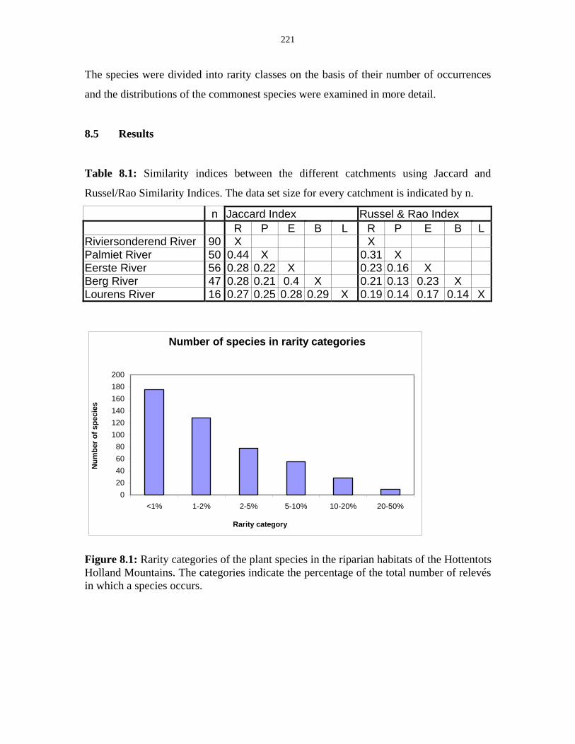
221
The species were divided into rarity classes on the basis of their number of occurrences
and the distributions of the commonest species were examined in more detail.
8.5 Results
Table 8.1: Similarity indices between the different catchments using Jaccard and
Russel/Rao Similarity Indices. The data set size for every catchment is indicated by n.
n Jaccard Index Russel & Rao Index R P E B L R P E B L
Riviersonderend River 90 X X Palmiet River 50 0.44 X 0.31 X Eerste River 56 0.28 0.22 X 0.23 0.16 X Berg River 47 0.28 0.21 0.4 X 0.21 0.13 0.23 X Lourens River 16 0.27 0.25 0.28 0.29 X 0.19 0.14 0.17 0.14 X
Number of species in rarity categories
020406080
100120140160180200
<1% 1-2% 2-5% 5-10% 10-20% 20-50%
Rarity category
Num
ber o
f spe
cies
Figure 8.1: Rarity categories of the plant species in the riparian habitats of the Hottentots Holland Mountains. The categories indicate the percentage of the total number of relevés in which a species occurs.
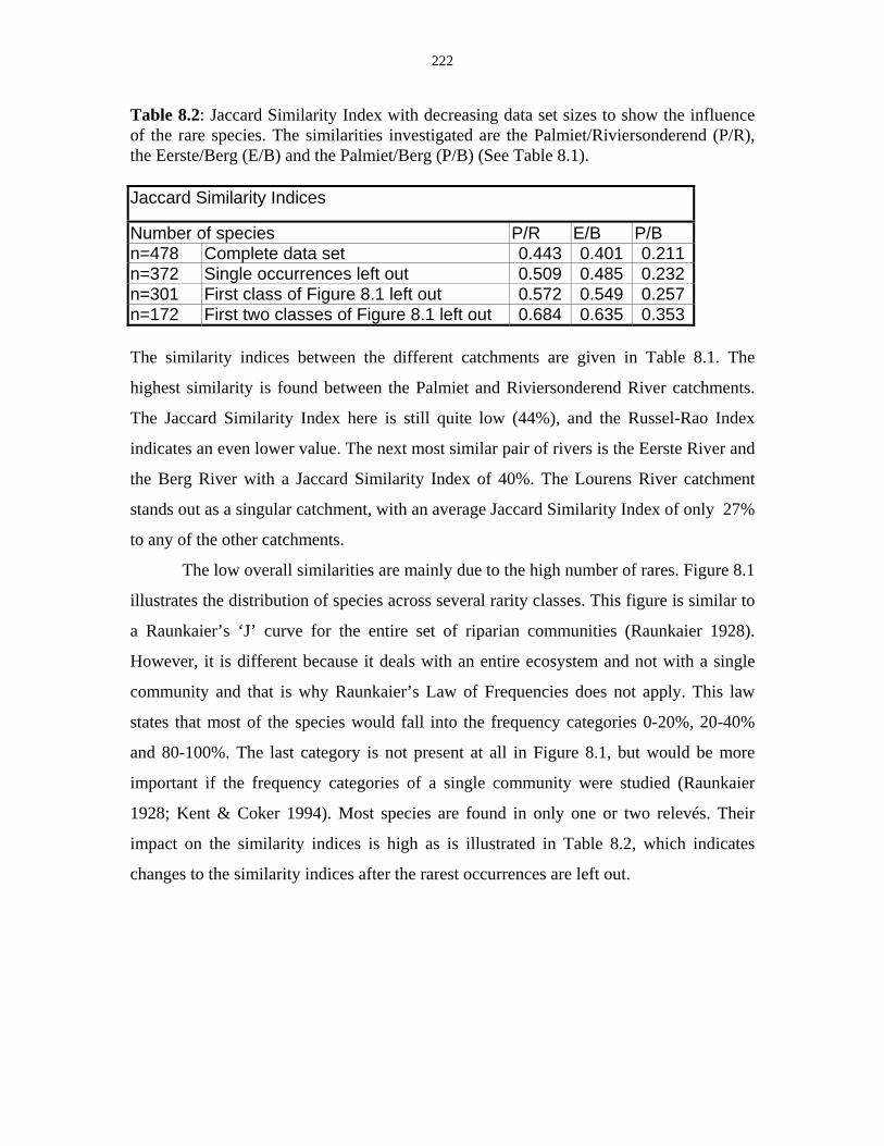
222
Table 8.2: Jaccard Similarity Index with decreasing data set sizes to show the influence of the rare species. The similarities investigated are the Palmiet/Riviersonderend (P/R), the Eerste/Berg (E/B) and the Palmiet/Berg (P/B) (See Table 8.1). Jaccard Similarity Indices
Number of species P/R E/B P/B n=478 Complete data set 0.443 0.401 0.211 n=372 Single occurrences left out 0.509 0.485 0.232 n=301 First class of Figure 8.1 left out 0.572 0.549 0.257 n=172 First two classes of Figure 8.1 left out 0.684 0.635 0.353 The similarity indices between the different catchments are given in Table 8.1. The
highest similarity is found between the Palmiet and Riviersonderend River catchments.
The Jaccard Similarity Index here is still quite low (44%), and the Russel-Rao Index
indicates an even lower value. The next most similar pair of rivers is the Eerste River and
the Berg River with a Jaccard Similarity Index of 40%. The Lourens River catchment
stands out as a singular catchment, with an average Jaccard Similarity Index of only 27%
to any of the other catchments.
The low overall similarities are mainly due to the high number of rares. Figure 8.1
illustrates the distribution of species across several rarity classes. This figure is similar to
a Raunkaier’s ‘J’ curve for the entire set of riparian communities (Raunkaier 1928).
However, it is different because it deals with an entire ecosystem and not with a single
community and that is why Raunkaier’s Law of Frequencies does not apply. This law
states that most of the species would fall into the frequency categories 0-20%, 20-40%
and 80-100%. The last category is not present at all in Figure 8.1, but would be more
important if the frequency categories of a single community were studied (Raunkaier
1928; Kent & Coker 1994). Most species are found in only one or two relevés. Their
impact on the similarity indices is high as is illustrated in Table 8.2, which indicates
changes to the similarity indices after the rarest occurrences are left out.
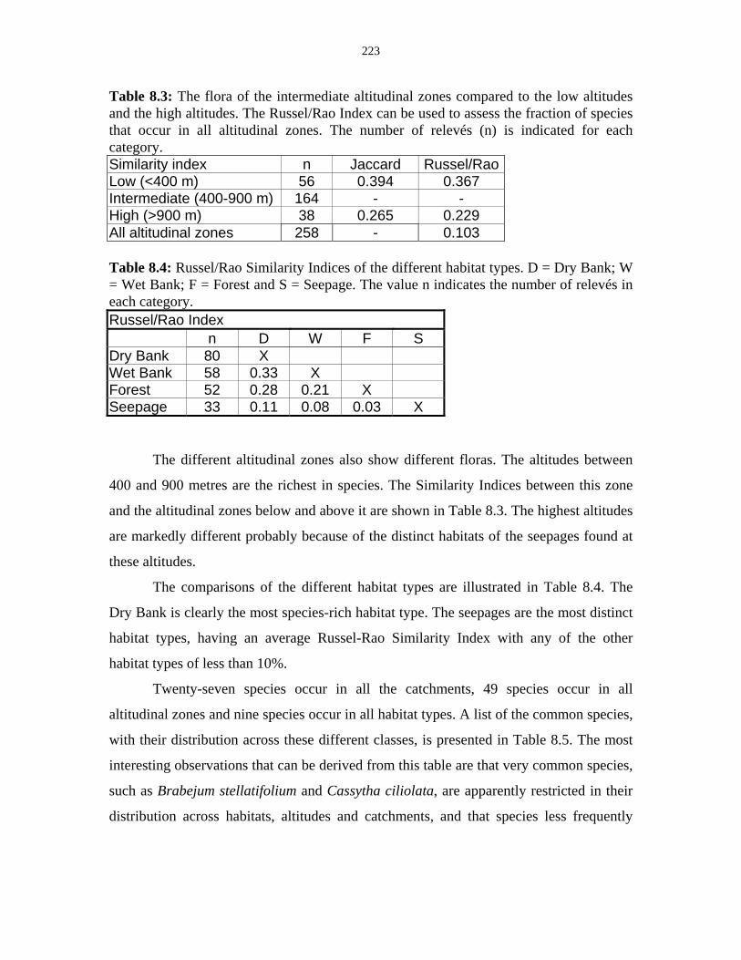
223
Table 8.3: The flora of the intermediate altitudinal zones compared to the low altitudes and the high altitudes. The Russel/Rao Index can be used to assess the fraction of species that occur in all altitudinal zones. The number of relevés (n) is indicated for each category. Similarity index n Jaccard Russel/RaoLow (<400 m) 56 0.394 0.367 Intermediate (400-900 m) 164 - - High (>900 m) 38 0.265 0.229 All altitudinal zones 258 - 0.103 Table 8.4: Russel/Rao Similarity Indices of the different habitat types. D = Dry Bank; W = Wet Bank; F = Forest and S = Seepage. The value n indicates the number of relevés in each category. Russel/Rao Index
n D W F S Dry Bank 80 X Wet Bank 58 0.33 X Forest 52 0.28 0.21 X Seepage 33 0.11 0.08 0.03 X
The different altitudinal zones also show different floras. The altitudes between
400 and 900 metres are the richest in species. The Similarity Indices between this zone
and the altitudinal zones below and above it are shown in Table 8.3. The highest altitudes
are markedly different probably because of the distinct habitats of the seepages found at
these altitudes.
The comparisons of the different habitat types are illustrated in Table 8.4. The
Dry Bank is clearly the most species-rich habitat type. The seepages are the most distinct
habitat types, having an average Russel-Rao Similarity Index with any of the other
habitat types of less than 10%.
Twenty-seven species occur in all the catchments, 49 species occur in all
altitudinal zones and nine species occur in all habitat types. A list of the common species,
with their distribution across these different classes, is presented in Table 8.5. The most
interesting observations that can be derived from this table are that very common species,
such as Brabejum stellatifolium and Cassytha ciliolata, are apparently restricted in their
distribution across habitats, altitudes and catchments, and that species less frequently
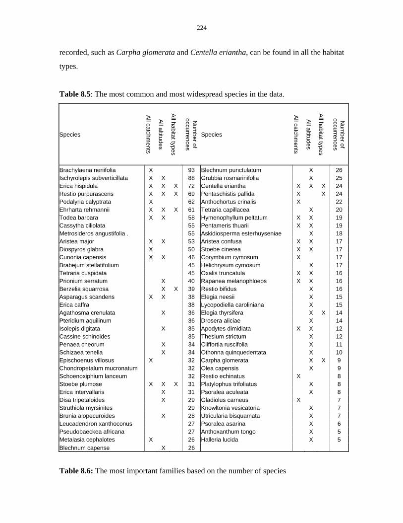
224
recorded, such as Carpha glomerata and Centella eriantha, can be found in all the habitat
types.
Table 8.5: The most common and most widespread species in the data.
Species
All catchm
ents
All altitudes
All habitat types
Num
ber of occurrences
Species
All catchm
ents
All altitudes
All habitat types
Num
ber of occurrences
Brachylaena neriifolia X 93 Blechnum punctulatum X 26 Ischyrolepis subverticillata X X 88 Grubbia rosmarinifolia X 25 Erica hispidula X X X 72 Centella eriantha X X X 24 Restio purpurascens X X X 69 Pentaschistis pallida X X 24 Podalyria calyptrata X 62 Anthochortus crinalis X 22 Ehrharta rehmannii X X X 61 Tetraria capillacea X 20 Todea barbara X X 58 Hymenophyllum peltatum X X 19 Cassytha ciliolata 55 Pentameris thuarii X X 19 Metrosideros angustifolia . 55 Askidiosperma esterhuyseniae X 18 Aristea major X X 53 Aristea confusa X X 17 Diospyros glabra X 50 Stoebe cinerea X X 17 Cunonia capensis X X 46 Corymbium cymosum X 17 Brabejum stellatifolium 45 Helichrysum cymosum X 17 Tetraria cuspidata 45 Oxalis truncatula X X 16 Prionium serratum X 40 Rapanea melanophloeos X X 16 Berzelia squarrosa X X 39 Restio bifidus X 16 Asparagus scandens X X 38 Elegia neesii X 15 Erica caffra 38 Lycopodiella caroliniana X 15 Agathosma crenulata X 36 Elegia thyrsifera X X 14 Pteridium aquilinum 36 Drosera aliciae X 14 Isolepis digitata X 35 Apodytes dimidiata X X 12 Cassine schinoides 35 Thesium strictum X 12 Penaea cneorum X 34 Cliffortia ruscifolia X 11 Schizaea tenella X 34 Othonna quinquedentata X 10 Epischoenus villosus X 32 Carpha glomerata X X 9 Chondropetalum mucronatum 32 Olea capensis X 9 Schoenoxiphium lanceum 32 Restio echinatus X 8 Stoebe plumose X X X 31 Platylophus trifoliatus X 8 Erica intervallaris X 31 Psoralea aculeata X 8 Disa tripetaloides X 29 Gladiolus carneus X 7 Struthiola myrsinites 29 Knowltonia vesicatoria X 7 Brunia alopecuroides X 28 Utricularia bisquamata X 7 Leucadendron xanthoconus 27 Psoralea asarina X 6 Pseudobaeckea africana 27 Anthoxanthum tongo X 5 Metalasia cephalotes X 26 Halleria lucida X 5 Blechnum capense X 26
Table 8.6: The most important families based on the number of species
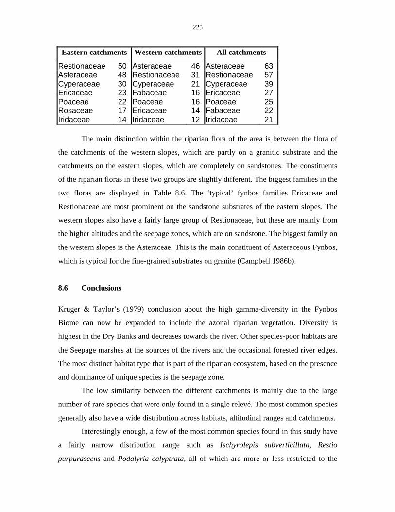
225
Eastern catchments Western catchments All catchments
Restionaceae 50 Asteraceae 46 Asteraceae 63 Asteraceae 48 Restionaceae 31 Restionaceae 57 Cyperaceae 30 Cyperaceae 21 Cyperaceae 39 Ericaceae 23 Fabaceae 16 Ericaceae 27 Poaceae 22 Poaceae 16 Poaceae 25 Rosaceae 17 Ericaceae 14 Fabaceae 22 Iridaceae 14 Iridaceae 12 Iridaceae 21
The main distinction within the riparian flora of the area is between the flora of
the catchments of the western slopes, which are partly on a granitic substrate and the
catchments on the eastern slopes, which are completely on sandstones. The constituents
of the riparian floras in these two groups are slightly different. The biggest families in the
two floras are displayed in Table 8.6. The ‘typical’ fynbos families Ericaceae and
Restionaceae are most prominent on the sandstone substrates of the eastern slopes. The
western slopes also have a fairly large group of Restionaceae, but these are mainly from
the higher altitudes and the seepage zones, which are on sandstone. The biggest family on
the western slopes is the Asteraceae. This is the main constituent of Asteraceous Fynbos,
which is typical for the fine-grained substrates on granite (Campbell 1986b).
8.6 Conclusions Kruger & Taylor’s (1979) conclusion about the high gamma-diversity in the Fynbos
Biome can now be expanded to include the azonal riparian vegetation. Diversity is
highest in the Dry Banks and decreases towards the river. Other species-poor habitats are
the Seepage marshes at the sources of the rivers and the occasional forested river edges.
The most distinct habitat type that is part of the riparian ecosystem, based on the presence
and dominance of unique species is the seepage zone.
The low similarity between the different catchments is mainly due to the large
number of rare species that were only found in a single relevé. The most common species
generally also have a wide distribution across habitats, altitudinal ranges and catchments.
Interestingly enough, a few of the most common species found in this study have
a fairly narrow distribution range such as Ischyrolepis subverticillata, Restio
purpurascens and Podalyria calyptrata, all of which are more or less restricted to the

226
extreme southwestern Cape (Goldblatt & Manning 2000). Other species are specific to
the Fynbos Biome riparian habitats, e.g. Brachylaena neriifolia, Prionium serratum and
Metrosideros angustifolia. Generalist plant species are a rare phenomenon in the Western
Cape.
227
9 Conclusions
9.1 Environmental aspects of riparian vegetation patterns in the Hottentots
Holland Mountains
The previous chapters dealt with several aspects about the riparian vegetation of the
Hottentots Holland Mountains. They dealt subsequently with the classification of
vegetation types, the impact of floods on the riparian zone, the environmental gradients
in the study area and biodiversity patterns along mountain streams. The situation in the
area reflects a nearly natural condition with minimal disturbance, so the vegetation types
resulting from classification can be used as reference types for bio-monitoring. The
seepage types described in Chapter 4 are probably very vulnerable to climatic change and
the riparian vegetation and the seepages can change due to water abstraction. It is
assumed that the vegetation will gradually change if the natural flood regime is
abandoned. This has been recorded in the lower reaches of rivers on many occasions
(Stevens et al. 1995; Tremolières et al. 1998). It is probably unique to the Fynbos Biome
that large-scale environmental gradients like climatic variation have the highest impact
on riparian vegetation. It can be questioned whether this impact would be similar in other
parts of the biome. But it is quite obvious that climatic aspects play a major role in the
maintenance of vegetation in the biome, even in vegetation types that seem to be
determined largely by other processes.
Although the vegetation patterns in the mountains are not as obvious as in the
lower reaches, the riparian zones identified by Boucher & Tlale (1999) can be maintained
in the highest reaches. The only riparian zone that is virtually non-existent in the
mountains is the Lower Dynamic Zone and if it is present it certainly does not support a
distinct vegetation type.
228
The riparian zonation can also be described as a continuum, as was done in
Chapter 7, but the results of this study support the notion of Glavaç et al. (1992) that
vegetation borders in riparian zones are generally very sharp. The hydrological and
hydraulic processes in rivers are very diverse, particularly in mountain streams where big
boulders, bedrock, woody debris, numerous bends, cascades and pools all have their
impact on local habitats. The local geomorphology determines whether the banks of a
river during a flood are mainly inundation-determined or stream power determined. If
inundation plays an important role, the vegetation will have to be adapted to a wet habitat
and to anaerobic conditions in the soil. If stream power plays an important role, the plants
growing on the river bank have to be adapted to mechanical disturbance and have a
strong rooting system. Because of all these influences, riparian zones are never really
extensive along the longitudinal axis and are broken up in many places, except in
stretches that are straight and without obvious changes in gradient. To summarize, one
can say that the dynamic nature of a river ecosystem is most obvious in a mountain
stream.
The riparian vegetation is part of the surrounding landscape and the
characteristics of a river are determined by processes in the catchment. In the Fynbos
Biome, where virtually every single mountain catchment forms a unique habitat with
endemic species, climatic and other large-scale processes play a major role. Every
catchment has its own riparian vegetation and this makes classification quite difficult at
this stage. Gradient analysis, as was done in Chapter 7, lends support to the classification
of the vegetation units.
Some concluding remarks will be derived here in order to deal with management
questions for riparian habitats in the mountains. At first it seems, that riparian habitats in
the mountains do not have many threats. After all, they are all safe within the borders of a
Nature Reserve or a Mountain Catchment Area and as long as the rest of the area is
managed well, the riparian zones will not experience many problems. On the other hand
there are some specific threats to riparian habitats that are dealt with here.
229
Alien vegetation
Rivers are quite susceptible to alien vegetation, because it is a habitat that is often
disturbed naturally and some of the Australian Acacia species are very common invaders
of riparian habitats. Alien vegetation also has its impact on the flow regime by
abstracting more water than the natural vegetation (Boucher & Marais 1995; Dye 1996).
The Working for Water Programme is a countrywide government programme that deals
with this threat by employing low-skilled workers to remove the alien vegetation
manually. This results in gains for water conservation, nature management and social
welfare. The Programme is also beneficial for education and skills development.
Handicraft products made from alien vegetation are sold locally and people are educated
to contribute to eco-tourism (pers. comm. D. Magadlela, Working for Water Programme).
There is potential to expand the Working for Water Programme with restoration projects
to bring the natural vegetation back in places where the alien Acacia’s have invaded the
entire riparian zone. The vegetation units described in this study and other riparian
studies (e.g. Brown & Day 1998; Boucher 1996) can be used as guidelines for such a
project.
It should be mentioned that within the study area, alien vegetation encroaching
into riparian zones is quite rare. The worst affected areas are Boesmans Kloof and
Banghoek Kloof. Alien vegetation consisting of pines is not specifically riparian but it is
a real threat on Franschhoek Peak and in Wesselsgat. The riparian vegetation just outside
the borders of the Nature Reserve is in a much worse condition. Here the rivers often
flow through pine plantations and the riverbanks are mostly vegetated by alien species. If
present management practices aimed at the control of alien vegetation are not continued,
the present relatively pristine nature of the mountain riparian vegetation could change
quite dramatically for the worse.
Flood regime
Based on arguments presented in Chapter 6 it is clear that inter-annual floods have an
important effect on riparian vegetation of mountain streams although they do not lead to
the same degree of diversification of habitats as they do in the lower reaches. The results
of Chapter 8 show however that the Dry Bank is the most species-rich riparian zone so
230
the inter-annual floods are very important to maintain species diversity in the riparian
zone. Riparian forests are poorer in species but form a distinct habitat especially for birds
but also for other animals. They are found in places that are sheltered from fire (Manders
et al. 1992) and they serve as a refuge for animals after a fire. The results of this study
suggest that they are not affected to any degree by the flood regime. However, it is likely
that they are mainly impacted upon by ground water level changes. Close to the river, the
ground water level is generally higher and this is probably one of the factors that enable
Afromontane Forests to grow here. The soil water regime is probably still the most
important factor that maintains a natural riparian ecosystem in the mountains. Water
abstraction in the mountains should be prohibited as far as possible to protect these
systems in a natural state.
The floods in the higher reaches will always have impact in the lower reaches, so
in a catchment-based management plan it is important to leave the upper reaches mostly
intact. Alterations to the original flow regime can only be partially corrected by other
tributaries that join the main stem downstream of the point of impoundment. More
information about the role of floods can be found in Ward & Stanford (1979).
Climatic regime
The above-mentioned management problems are easily controlled, because they mainly
operate at a small scale, within the borders of the nature reserve. In Chapter 7 it can be
seen that large-scale environmental factors have an impact on vegetation that is just as
high or even higher than small-scale environmental factors. Conservationists within a
nature reserve are mostly concerned with small-scale processes that can be controlled
within the reserve, but in the case of fynbos and its sharp environmental gradients,
sufficient attention must also be paid to the large-scale processes that the reserve is
subjected to. It is difficult for managers to make a positive impact on the large-scale
environmental processes, although other people, mainly in the cities, do not have many
problems in affecting them negatively. Only an awareness campaign about the
environmental problems aimed at changing the behaviour of people and their use of
water, energy and waste can influence things in this respect. Global warming and the
resulting desertification will have a high impact on the Fynbos Biome and all its
231
vegetation types (Rutherford et al. 1999). Monitoring programmes should be set up in
order to follow the changes and assess their severity. The wet habitats, that are the most
vulnerable, should be monitored carefully and more weather stations should be set up on
the tops of the mountains. These wet habitats contain many endemic species and are the
sources of our drinking water so they are of great importance.
The mountain stream in a fynbos environment
In all other respects, riverine vegetation should be managed as a part of the entire
mountain catchment. It is situated within the Mountain Fynbos, which implies that it
occurs in a fire-prone environment. Most riparian species do not have specific fire
responses like serotiny or fire-induced flowering. However, if one has a look at the
riparian vegetation after a fire, it appears that this vegetation does not burn readily. Only
the Back Dynamic Zone is really fire-prone, but the other zones are mostly protected
because of the wet habitat, the seemingly low flammability levels of the vegetation or the
low density of the vegetation in the Wet Banks. After a fire, the runoff in rivers increases
with rains (Bosch & Versfeld 1982) and the rivers are then prone to flooding, which
enlarges the wet habitat. Dense stands of exotic Acacia plants can change the situation
and increase the fuel load, the fire temperatures and the fire intensity on the river bank
and thus increase the probability that naturally protected areas will burn as well (Versfeld
& Van Wilgen 1986). Many riparian habitats are also naturally sheltered from fires, for
example when they are located in steep gorges. In some cases, riparian habitats act as
‘natural fire-breaks’ protecting large pieces of fynbos from fire. In the 1999 fire in the
Hottentots Holland Mountains, a part of the Boegoekloof did not burn, because it was
enclosed between two gorges, a steep slope of Victoria Peak, and the Riviersonderend
River. Such areas serve as refuges for animals and plants during and after the fire, in
addition to the riparian habitats themselves.
A problem starts when man-made fires are ignited in the riparian vegetation,
when the fuel load is larger such as after felling alien plants. This should never be done,
because the riparian vegetation is not adapted to survive hot fires.
For the rest, fire management does not have to take riparian vegetation into
account. Riparian vegetation seems to be able to protect itself against fires and the
232
vegetation is only affected by very intense fires. In managed fires, the riparian zones
should be avoided, particularly if very intense fires could result.
9.2 The future of phytosociological research in the Fynbos Biome
The VEGMAP project (McDonald 1997; Mucina et al. 2000) has for the first time
compiled all the vegetation data that is available in the Fynbos Biome into a single
database. One of the clear messages that has come out of this compilation is that the
Fynbos Biome is seriously undersampled. The consequences of the VEGMAP project for
the documentation of vegetation types in the Fynbos Biome have been assessed by
McDonald & Boucher (1999). The completion of this study of riverine vegetation offers
a good opportunity to evaluate the directions that phytosociological research in the
Fynbos Biome has to take. The times have changed since Taylor (1969), Boucher (1972)
and Werger et al. (1972) made the first efforts to apply the Braun-Blanquet method in the
Fynbos Biome, but it has now been proven beyond doubt that this method can be used
successfully in the Fynbos Biome.
What is even more, the method has been applied to nearly all species-rich
vegetation types in the tropics and subtropics and it is nowadays, in combination with
gradient analysis, generally accepted as a scientific standard for studying vegetation
(Kent & Coker 1992). And yet, in most parts of the world, except in Europe where the
Braun-Blanquet method originated, the final steps of creating a hierarchical system are
still largely non-existent. This is in many cases due to a shortage of data and this applies
particularly to the Fynbos Biome.
Since Campbell (1985, 1986a, 1986b) wrote his elaborate report on the structural
subdivision of Mountain Fynbos, an ongoing discussion about the feasibility of applying
the Braun-Blanquet method on a wide scale in the Fynbos Biome has been started
(Boucher 1987; McDonald & Boucher 1999). It is a pity that this discussion has in
certain ways blocked the ongoing collection of phytosociological data, while Campbell’s
(1986b) structural classification itself is very useful as a first comprehensive draft to
tackle this very complex vegetation. I think that by now, the focus in this discussion
should be shifted. Theoretically, a phytosociological classification of the Fynbos Biome

233
is very feasible, but it will not happen overnight. The discussion should focus now on
which vegetation types are undersampled and should have preference to be surveyed.
Before I continue my demonstration, I want to look at the reasons why the Braun-
Blanquet method was so successful in Europe and comment on the differences from the
situation in Africa. As in other disciplines of science that Europeans introduced to Africa
it is important to find ‘an African solution for African problems’, without disregarding
scientific standards.
A complete survey of all vegetation types did not happen overnight in Europe,
just as it will not happen rapidly in South Africa. By the time Europe started to study its
vegetation, a large portion of land had already been transformed. The processes of
exploitation of the vegetation and the description of it went hand in hand. The ‘islands’ of
natural areas that are left behind, are also ‘exploited’ for recreational purposes, nature
conservation and nature study. One must not forget that a vegetation association, like its
taxonomic equivalent the species, is basically a human construct. For a large portion of
the European population it was easy to visit the ‘remnant’ natural areas and see the
vegetation types that were described, so a ‘concept’ of these vegetation types developed
in the minds of not only the scientists but also of other people who were concerned about
the survival of natural vegetation. As a result, syntaxonomic description and
classification of the vegetation found a broad support base among the whole society.
These are some of the considerations I would like to take to the South African
context. What one must bear in mind is that phytosociology, like all natural sciences does
not necessarily say as much about its subject, vegetation, as it does about ourselves. It has
always been the elements in nature that live in a close relationship with the human
species that receive the most attention. However much we try to be objective in science,
we always come back to these same species, ecosystems or processes, while others, that
are ‘scientifically’ just as interesting, seem to escape our devotion forever.
When it comes to the classification of Mountain Fynbos, we must consider that
there is no way that we can claim a special ‘scientific’ importance in descriptive sciences
like vegetation science. This importance is determined by ourselves and the relation that
we as a society have with the object of our study. Fynbos itself does not care about how it
is classified, so as long as there is no base of interest among a significant part of the
234
population, Mountain Fynbos will just remain Mountain Fynbos and nothing more. Even
if there is a more detailed subdivision that is used by a small group of scientists, if the
concept of this vegetation type does not ‘come alive’ among a broader base, like nature
conservationists, amateurs, and scientists of other disciplines, like geologists,
agriculturalists and plant taxonomists, it is questionable whether the classification has
achieved its aim. The CAPE project (Cape Action Plan for the Environment), currently
launched in the Western Cape (World Wildlife Fund – South Africa 2000), will provide a
good opportunity not only to do more research in the field, but also to carry the
phytosociological knowledge out to other disciplines.
The way we look at our vegetation is also mostly determined by our direct
environment. Someone living in a desert will develop a completely different
understanding of the concept of vegetation from someone else living in a tropical
rainforest. The concept of classification originated in Europe, while in America the
approach of gradient analysis was preferred (Whittaker 1967). Also in Australia, much
attention was paid to environmental gradients (for example Austin 1987). Westhoff & De
Smidt (1995) point out that this is a logical outcome of the local situation. In America,
vast stretches of natural vegetation were still present at the time when the vegetation
research started, which made the natural gradients that occurred much more obvious. The
reason why the approach of classification found more appeal in Europe is because the
vegetation there was already present in remnant pieces that could be classified with more
ease. It should be noted that the original form of ordination was developed by a Russian
vegetation scientist, Ramenski, who also lived in a country where large areas of natural
vegetation remained as in America (Sobolov & Utekhin 1973).
South Africa, considering its vast stretches of unaffected vegetation, its strong
gradients and the complexity of its vegetation, actually chose the wrong approach. Most
of the focus has been on the classification of vegetation, mainly because of the stronger
cultural links with Europe and the influence of Dutch phytosociologists like M.J.A
Werger, E.M. van Zinderen Bakker and F. van der Meulen. However, the vegetation
itself is more suitable to use approaches of ordination, but multivariate techniques have
so far received relatively little attention in the country. Canonical Correspondence
Analysis is still rarely used, while it is a very good technique to reveal the complex
235
processes underlying most of the country’s vegetation gradients. The combination of
constrained and unconstrained ordination the way Økland (1994) proposes is only used
very rarely.
It does not mean that multivariate techniques are the one and only answer for the
vegetation in South Africa. Since the seventies it is common practice to use both
classification and ordination in vegetation studies, because both of them reveal certain
characteristics in the vegetation (Whittaker 1972; Van der Maarel 1975). Because of the
complexity of the vegetation, however, it is likely that ordination will provide more
information in the initial stages that might prove more useful for conservation as well.
The underlying structure of a hierarchical classification only becomes apparent if the data
set becomes significantly large. Data collection in the Fynbos Biome should continue to
happen, even though the long-term goal of a hierarchical classification is not yet
achievable. On the other hand, the short-term goal is to get an overview and an
understanding of the ecological processes affecting the fynbos vegetation. The collection
of phytosociological data is part of this process, because relevé data can be used in many
analyses afterwards and it forms the most efficient way of data collection. The focus
should be with the environmental aspects and not just with the description of the
vegetation.
In my view, the vegetation types that should be given priority in sampling are
mainly those which have a special relationship with human society or those that are most
threatened. Of both types I will mention some specific examples:
- Riparian vegetation: this vegetation has a specific relationship with human
society, because it plays a major role in the exploitation of our drinking water
and it can be affected by the way we abstract that water. And on top of that
there are thousands of South Africans who have their daily work in the
riparian vegetation and would like to monitor the results of their efforts: the
participants in the Working for Water Project.
- The coastal vegetation: this vegetation suffers a great impact from the
populace because of mass recreation and it has specific threats because of
coastal development.
236
- Ecotourism areas: for example the area of the Kogelberg Biosphere Reserve
and the proposed West Coast Biosphere Reserve. There should be sufficient
understanding of the ecological processes in areas that expect high numbers of
tourists, because of the conservation priorities. Much interest in the vegetation
can be expected from the tourists themselves and the people who make their
living out of ecotourism.
- The habitats of economically important species: These habitats should be
conserved as a gene pool for the economically important species such as
rooibos (Aspalathus linearis), boegoe (Agathosma betulina / A. crenulata) and
proteas (Protea ssp. and Leucospermum ssp.).
- Lowland Renosterveld and Sandplain Fynbos: these are the most threatened
habitats because they have mostly been transformed for agriculture or
urbanization. For effective conservation of these habitats, virtually every
remnant patch of these vegetation types should get some conservation status.
For eventual restoration purposes, it would be advisable to collect as much
information about these habitats as possible.
- Wet habitats in the mountains and in the lowlands: these are quite susceptible
to climate change, which might play a bigger role in the Fynbos Biome in the
future.
The CAPE project, launched in September 2000 in Cape Town, promotes research into
the biodiversity of the Fynbos Biome in combination with the sustainable use of
resources and strengthening of institutions (World Wildlife Fund – South Africa 2000).
Phytosociology will play a major role in this new stimulation of fynbos research. In
combination with synecology it can provide many answers to questions about ecological
processes and the autecology of single species. The vegetation data itself can be used as a
reference in monitoring or restoration projects. The Braun-Blanquet method offers the
most efficient way to collect and store vegetation data and can offer the CAPE Project a
great service.
The phytosociological work to be done in the Fynbos Biome before a hierarchical
classification is feasible, seems immense. If work is focused on a few priority areas an

237
overview of the task will be achievable. The work presented in this thesis does not mean
an end to the research on riparian vegetation in the Fynbos Biome: it is just the
beginning. However, it offers a good basis for riparian vegetation classification and the
ecological processes that operate on riparian communities. One day, an overview of all
riparian vegetation types in the Biome will be feasible.

238
References
239
Acocks, J.P.H., 1953. Veld types of South Africa. Mem. Bot. Surv. S. Afr. No. 28.
Acocks, J.P.H., 1975. Veld types of South Africa. 2nd ed. Mem. Bot. Surv. S. Afr. No.
40.
Acocks, J.P.H., 1988. Veld types of South Africa. 3rd ed. Mem. Bot. Surv. S. Afr. No.
57.
Adamson, R.S., 1938. The vegetation of South Africa. British Empire Vegetation
Committee, London.
Adamson, R.S., 1958. The Cape as an ancient African flora. Advmnt. Sci. 58: 1-10.
Alexander, W.J.R., 1991. Flood hydrology for Southern Africa. South African National
Committee on large dams, Pretoria.
Allen, T.F.H., 1987. Hierarchical complexity in ecology: a non-euclidian conception of
the data space. Vegetatio 69: 17-25.
Anonymous, 1990. Handbook of standard soil testing methods for advisory purposes.
Soil Science Society of South Africa, Pretoria.
Anonymous, 1999. The Working for Water Programme. 1998/99 Annual Report.
Austin, M.P., 1987. Models for the analysis of species’ reponse to environmental
gradients. Vegetatio 69: 35-45.
Austin, M.P., Cunningham, R.B. & Fleming, P.M., 1984. New approaches to direct
gradient analysis using environmental scalars and statistical curve-fitting
procedures. Vegetatio 55: 11-27.
Austin, M.P. & Gaywood, M.J., 1994. Current problems of environmental gradients and
species response curves in relation to continuum theory. J. Veg. Sci. 5: 473-482.
Austin, M.P., Nicholls, A.O., Doherty, M.P. & Meyers, J.A., 1994. Determining
species response functions to an environmental gradient by means of a ß-function.
J. Veg. Sci. 5: 215-228.
Austin, M.P. & Smith, T.M., 1989. A new model for the continuum concept. Vegetatio
83: 35-47.
Ball, D.F., 1986. Site and soils. In: Moore, P.D. & Chapman, S.B. (eds.) Methods in
Plant Ecology, 2nd ed., Blackwell Scientific Publications, Osney Mead, Oxford.
Barkman, J.J., 1989. A critical evaluation of minimal area concepts. Vegetatio 85: 89-
104
240
Barkman, J.J., Doing, H. & Segal, S., 1964. Kritische Bemerkungen und Vorschläge
zur qualitativen Vegetationskunde. Acta Bot. Neerl. 13: 394-419.
Beekhuis, J., Bekker, C.T., Joubert, S.J. & Marwick, C.W., 1944. Some geomorphic
aspects of the Eerste River system. Ann. Univ. Stellenbosch 22. Section. A: 239-
248.
Bendix, J., 1999. Stream power influence on southern Californian riparian vegetation. J.
Veg. Sci. 10, 2: 243-252.
Bews, J.W., 1916. An account of the chief types of vegetation in South Africa, with
notes on the plant succession. J. Ecol. 4: 129-159.
Birkhead, A.L., Olbrich, B.W., James, C.S. & Rogers, K.H., 1996. Developing an
integrated approach to predicting water use of riparian vegetation. Report No.
474/1/96. Water Research Commission, Pretoria.
Bolus, H., 1886. Sketch of the flora of South Africa. In: Official Handbook of the Cape
of Good Hope. Richards, Cape Town.
Bolus, H., 1905. Sketch of the floral regions of South Africa. In: Flint,W. & Gilchrist,
J.D.F. (eds.) Science in South Africa pp. 199-240. Maskew Miller, Cape Town.
Bond, W.J., 1981. Vegetation gradients in Southern Cape Mountains. M.Sc. thesis,
Univ. Cape Town, Rondebosch.
Bond, W.J., 1997. Fire. In: Cowling, R.M., Richardson, D.M. & Pierce, S.M. (eds.),
Vegetation of Southern Africa, Cambridge University Press, Cambridge.
Bond, P. & Goldblatt, P., 1984. Plants of the Cape Flora, A descriptive catalogue. J. S.
Afr. Bot., Supplement No. 13.
Borcard, D., Legendre, P. & Drapeau, P., 1992. Partialling out the spatial component
of ecological variation. Ecol. 73, 3: 1045-1055.
Bosch, J.M. & Versfeld, D.B., 1982. Forestry and the management of riparian zones.
Unpublished Report. Jonkershoek Forestry Research Centre, Department of
Environment Affairs.
Bosch, J.M., Alletson, D.J., Jacot Guillarmod, A.F.M.G., King, J.M. & Moore, C.A.,
1986. River response to catchment conditions. In: O’Keeffe, J.H. (ed.): the
conservation of South African rivers. S. Afr. Nat. Sci. Prog. Rep. No. 131.
241
Boucher, C., 1972. The vegetation of the Cape Hangklip area. M.Sc. thesis, Univ. Cape
Town, Rondebosch.
Boucher, C., 1978. Cape Hangklip area. II. The vegetation. Bothalia 12, 3: 455-497.
Boucher, C., 1987. A phytosociological study of transects through the Western Cape
Coastal Foreland, South Africa. Ph.D. Thesis, Univ. Stellenbosch, Stellenbosch.
Boucher, C. 1996. The vegetation of the Berg River with particular reference to the
DWAF IFR sites. Unpublished Report to the Skuifraam Feasibility Study,
Department of Water Affairs and Forestry.
Boucher, C. & Moll, E.J., 1981. South African mediterranean shrublands. In: Di Castri,
F., Goodall, D.W. & Specht, R.L.(eds.). Ecosystems of the World 11,
Mediterranean-type shrublands. Elsevier, Amsterdam.
Boucher, C. & Marais, C. (eds.), 1995. Managing Fynbos Catchments for Water,
Proceedings of a workshop held on 30 November 1993 at Stellenbosch, South
Africa. Foundation for Research & Development Report Series No. 24.
Boucher, C. & Tlale, S., 1999. Riparian and instream vegetation study. Unpublished
Report prepared for Lesotho Highlands Development Authority, Lesotho Highlands
Water Project. Metsi Consultants, Maseru.
Bowman, D.M.J.S. & McDonough L., 1991. Tree species distribution across a
seasonally flooded elevation gradient in the Australian monsoon tropics. J.
Biogeogr. 18: 203-212.
Bragazza, L. & Gerdol, R., 1999. Hydrology, groundwater chemistry and peat
chemistry in relation to habitat conditions in a mire on the South-eastern Alps of
Italy. Plant Ecol. 144: 243-256.
Bray, J.R. & Curtis, J.T., 1957. An ordination of the upland forest communities of
southern Wisconsin. Ecol. Monogr. 27: 325-349.
Braun-Blanquet, J., 1921. Prinzipien einer Systematik der Pflanzengesellschaften auf
floristischer Grundlage. Jahrb. St. Gallen Naturw. Ges. 57: 305-351.
Braun-Blanquet, J., 1928. Pflanzensoziologie. Grundzüge der Vegetationskunde.
Biologischer Studienbücher 7. 1. Ed. Berlin.
242
Brinson, M.M., 1990. Riverine forests. In: Lugo, A.E., Brinson, M.M. & Brown, S.
(eds.). Ecosystems of the World No. 16. Forested Wetlands. Elsevier, Amsterdam.
Brown, A., Birks, H.J.B. & Thompson, D.B.A., 1993. A new biogeographical
classification of the Scottish uplands. II. Vegetation-environment relationships. J.
Ecol. 81: 231-251.
Brown, C.A. & Dallas, H.F., 1995. Eerste River, Western Cape, Situation assessment of
the riverine ecosystem. Unpublished report prepared for Southern Waters, Cape
Town.
Brown, C.A. & Day, E., 1998. IFR Starter Document, Assessment of the Instream Flow
Requirements for the Palmiet River and the Freshwater Requirements for the
Palmiet Estuary. Unpublished report prepared for Southern Waters, Cape Town.
Burgers, C.J., 1992. The conservation status of the riverine vegetation and habitats of
the Berg River between Franschhoek and Zonquasdrift. Unpublished report
prepared for the Dept. of Water Affairs worksession on the Instream Flow
Requirements of the Upper Berg River, held at Noordhoek on 12 / 13 November
1992.
Campbell, B.M., 1983. Montane plant environments in the Fynbos Biome, Bothalia 14,
2: 283-298.
Campbell, B.M., 1985. Montane vegetation structure in the Fynbos Biome. Doctoral
thesis, Rijks University Utrecht, Utrecht.
Campbell, B.M., 1986a. Vegetation classification in a floristically complex zone: the
Cape Floristic Region. S. Afr. J. Bot. 52, 2: 129-140.
Campbell, B.M., 1986b. A classification of the mountain vegetation of the Fynbos
Biome. Mem. Bot. Surv. S. Afr. 50.
Campbell, B.M. & Moll, E.J., 1977. The forest communities of Table Mountain, South
Africa. Vegetatio 34, 2: 105-115.
Cape Nature Conservation, 1994. Boland Hiking Trail, Hottentots Holland Section, 3rd
edition. Cape Nature Conservation, Jonkershoek.
Clements, F.E., 1916. Plant succession. An analysis of the development of vegetation.
Carnegie Institute, Publication 242, Washington D.C.
Clements, F.E., 1928. Plant succession and indicators. Wilson, New York.
243
Cowling, R.M., 1984. A syntaxonomic and synecological study in the Humansdorp
Region of the Fynbos Biome. Bothalia 15: 175-227.
Cowling, R.M. & Hilton-Taylor, C., 1997. Phytogeography, flora and endemism. In:
Cowling, R.M., Richardson, D.M. & Pierce, S.M. (eds.), Vegetation of Southern
Africa, Cambridge University Press, Cambridge.
Cowling, R.M. & Holmes, P.M., 1992. Flora and vegetation. In: Cowling, R.M. (ed.),
The ecology of fynbos; nutrients, fire and diversity. Oxford University Press, Cape
Town.
Cowling, R.M., Holmes, P.M. & Rebelo, A.G., 1992. Plant diversity and endemism. In:
Cowling, R.M. (ed.), The ecology of fynbos; nutrients, fire and diversity. Oxford
University Press, Cape Town.
Cowling, R.M., Richardson, D.M. & Mustart, P.J., 1997. Fynbos. In: Cowling, R.M.,
Richardson, D.M. & Pierce, S.M. (eds.), Vegetation of Southern Africa, Cambridge
University Press, Cambridge.
Crabtree, N.M. & Trudgill, S.T., 1985. Hillslope hydrochemistry and stream response
on a wooded permeable bedrock: the role of stemflow. J. Hydrol. 80: 161-178.
Curtis, J.T. & McIntosh, R.P., 1951. An upland forest continuum in the prairie-forest
border region of Wisconsin. Ecol. 32: 476-496.
Davies, B.R. & Day, J.A., 1989. Physical and chemical attributes important in the
biological functioning of river ecosystems. In: Ferrar, A.A. (ed.), Ecological flow
requirements for South African rivers. S. Afr. Nat. Sci. Prog. Rep. No. 162.
Davies, B.R. & Day, J.A., 1998. Vanishing waters. University of Cape Town Press,
Rondebosch.
Davies, B.R., O’Keeffe, J.H. & Snaddon, C.D., 1993. A synthesis of the ecological
functioning, conservation and management of South African river ecosystems.
Water Reseach Commission Report no. TT 62/93.
Day, J.H. (ed.), 1981. Estuarine ecology with particular reference to Southern Africa.
A.A. Balkema, Cape Town.
Day, J.A., Davies, B.R. & King, J.M., 1986. Riverine ecosystems. In: O’Keeffe, J.H.
(ed.), The conservation of South African rivers. S. Afr. Nat. Sci. Prog. Rep. No.
131.
244
Deacon, H.J., Jury, M.R. & Ellis, F., 1992. Selective regime and time. In: Cowling,
R.M. (ed.), The ecology of fynbos; nutrients, fire and diversity. Oxford University
Press, Cape Town.
Deacon, H.J., 1992. Human settlement. In: Cowling, R.M. (ed.), The ecology of fynbos;
nutrients, fire and diversity. Oxford University Press, Cape Town.
Decocq, G., 2002. Patterns of plant species and community diversity at different
organization levels in a forested riparian landscape. J. Veg. Sci. 13: 91-106.
De Lange, C., 1992. Floristic analysis of the Vogelgat Nature Reserve, Cape Province,
South Africa. M.Sc. Thesis, University of Cape Town, Rondebosch.
Dent, M.C., Lynch, S.D. & Schulze, R.E., 1987. Mapping mean annual precipitation
and other rainfall statistics over Southern Africa. Agricultural Catchments Research
Unit Report No. 27. Water Research Commission Report No. 109/1/89.
Department of Water Affairs & Forestry, 1994. In-stream Flow Requirements of the
Berg River from Skuifraam Dam Site to Zonquasdrift. Volume I: Proceedings of
Worksessions. Western Cape System Analysis, Ninham Shand, Cape Town.
Department of Water Affairs & Forestry, 1996. Skuifraam Feasibility Study. Berg
River IFR Refinement Worksession. Unpublished Report.
De Villiers, J., Jansen, H. & Mulder, M.P., 1964. Die geologie van die gebied tussen
Worcester en Hermanus. Geological Survey, Pretoria.
Dixon, M.D. & Johnson, W.C., 1999. Riparian vegetation along the middle Snake
River, Idaho: zonation, geographical trends and historical changes. Great Basin
Naturalist 59, 1: 18-34.
Du Toit, A., 1998. Verspreiding en digtheid van Prionium serratum (L.f.) Drege ex E.
Mey. langs die Eerste Rivier. Hons. Project, Univ. Stellenbosch, Stellenbosch.
Dye, P.J., 1996. Climate, forest and streamflow relationships in South African afforested
catchments. Commonwealth For. Rev. 75, 1: 31-38.
Eastman, J.R., 1997. IDRISI for Windows, User’s Guide, Version 2.0, IDRISI
production, Clark University, MA, USA.
Edwards, D., 1983. A broad-scale structural classification of vegetation for practical
purposes. Bothalia 14, 3 & 4: 705-712.
245
Emberger, L., 1955. Projet d’une classification biogeographque des climats. In: Les
divisions écologiques du monde, C.N.R.S., Paris. 5-11.
Featherstone, R.E. & Nalluri, C., 1995. Civil engineering hydraulics. Blackwell
Science Ltd., Oxford, United Kingdom.
Feoli, E. & Orloci, L., 1985. Analysis of concentration and detection of underlying
factors in structured tables. Vegetatio 40, 1: 49-54.
Ferrar, A.A., O’Keeffe, J.H. & Davies, B.R., 1988. The River Research Programme, S.
Afr. Nat. Sci. Prog. Rep. No. 146.
Fetherston, L.F., Naiman, R.J. & Bilby, R.E., 1995. Large woody debris, physical
process, and riparian forest development in montane river networks of the Pacific
Northwest. Geomorph. 13: 133-144.
Franz, E.H. & Bazzaz, F.A., 1977. Simulation of vegetation response to modified
hydrologic regimes: A probalistic model based on niche differentiation in a
floodplain forest. Ecol. 58: 176-183.
Fry, M. St. L., 1987. A detailed characterization of soils under different fynbos-climate-
geology combinations in the south-western Cape. M.Sc. thesis, University of
Stellenbosch, Stellenbosch.
Fuggle, R.F., & Ashton, E.R., 1979. Climate. In: Day, J., Siegfried, W.R., Louw, G.N.
& Jarman, M.L. (eds.), Fynbos ecology: a preliminary synthesis. S. Afr. Nat. Sci.
Prog. Rep. No. 40.
Furness, H.D. & Breen, C.M., 1980. The vegetation of seasonally flooded areas of the
Pongolo River Floodplain. Bothalia 13, 1 & 2: 217-231.
Gauch, H.G. Jr., 1982. Multivariate analysis in community ecology. Cambridge
University Press, Cambridge.
Geldenhuys, C.J., 1997. Composition and biography of forest patches on the inland
mountains of the Southern Cape. Bothalia 27, 1: 57-74.
Glavaç, V., Grillenberger, C., Hakes, W. & Ziezold, H., 1992. On the nature of
vegetation boundaries, undisturbed flood plain forest communities as an example -
a contribution to the continuum/discontinuum controversy. Vegetatio 101: 123-144.
Gleason, H.A., 1917. The structure and development of the plant association. Bull.
Torrey Bot. Club 43: 463-481.
246
Gleason, H.A., 1926. The individualistic concept of the plant association. Bull. Torrey
Bot. Club 52: 1-20.
Gleason, H.A., 1939. The individualistic concept of the plant association. Amer. Midl.
Nat. 21: 92-110.
Glyphis, J., Moll, E.J. & Campbell, B.M., 1978. Phytosociological studies on Table
Mountain, South Africa. 1. The Back Table. J. S. Afr. Bot. 44, 3: 281-289.
Goldblatt, P., 1978. An analysis of the flora of Southern Africa: its characteristics,
relationships and origins. Ann. Missouri Bot. Gard. 65: 369-436.
Goldblatt, P. & Manning, J., 2000. Cape plants. A conspectus of the Cape flora of
South Africa. Strelitzia 9.
Good, R., 1974. The geography of the flowering plants. 4th ed. Longman, London.
Goodall, D.W., 1973. Numerical classification. In: Whittaker, R.H. (ed.), Ordination and
classification of communities. Manual of Vegetation Science 6. Junk, The Hague.
Gordon, N.D., McMahon, T.A. & Finlayson, B.I., 1992. Stream hydrology. An
introduction for ecologists. John Wiley & Sons, New York.
Gore, A.J.P., 1983. Introduction. In: Gore, A.J.P. (ed.) Ecosystems of the world 4A:
Mires: Swamp, Bog, Fen and Moor, General Studies. Elsevier, Amsterdam.
Gregory, S.V., Swanson, F.J., McKee, W.A. & Cummins, K.W., 1991. An ecosystem
perspective of Riparian zones. Focus on links between land and water. Bioscience
41: 540-551.
Hancock, C.N., Ladd, P.G. & Froend, R.H., 1996. Biodiversity and management of
riparian vegetation in Western Australia. For. Ecol. & Manag. 85: 239-250.
Heap, P., 1993. The story of Hottentots Holland. 3rd edition. Peggy Heap, Somerset
West.
Hennekens, S.M., 1996. MEGATAB - a visual editor for phytosociological tables.
Version 1.0, October 1996. Giesen & Geurts, Ulft.
Hennekens, S.M., 1998. Turboveg for Windows 1.93e. International single user version.
1998-2000. Stefan Hennekens.
Hewlett, J.D., 1961. Soil moisture as a source of base flow from steep mountain
watersheds. S.E. Expt. Stat., USDA Forest Service Paper 132.
247
Hewlett, J.D., 1982. Principles of forest hydrology. University of Georgia Press, Athens,
Georgia, USA.
Hewlett, J.D. & Hibbert, A.R., 1967. Factors affecting the response of small watersheds
to precipitation in humid areas. In: Sopper, W.E. & Lull, H.W. (eds.) International
Symposium on Forest Hydrology, pp. 275-290. Pergamon Press, Oxford.
Hill, M.O., 1973. Reciprocal averaging: an eigenvector method of ordination. J. Ecol. 61:
237-249.
Hill, M.O., 1974. Correspondence analysis: a neglected multivariate method. Appl. Stat.
23: 340-354.
Hill, M.O., 1979. TWINSPAN - a FORTRAN Program for arranging multivariate data in
an ordered two way table for classification of the individuals and the attributes.
Cornell University, Department of Ecology and Systematics, Ithaca, New York.
Hill, M.O. & Gauch, H.G., 1980. Detrended correspondence analysis: an improved
ordination technique. Vegetatio 42: 47-58.
Huntley, B.J., 1992. The Fynbos Biome Project. In: Cowling, R.M. (ed.), The ecology of
fynbos; nutrients, fire and diversity. Oxford University Press, Cape Town.
Hupp, C.R., 1988. Plant ecological aspects of flood geomorphology and paleoflood
history. In: Baker, R., Kochel, R.C. & Patton, P.C. (eds.) Flood geomorphology,
pp. 335-356. John Wiley & Sons, New York.
Hupp, C.R. & Osterkamp, W.R., 1985. Bottomland vegetation distribution along
Passage Creek, Virginia, in relation to fluvial landforms. Ecol. 66, 3: 670-681.
Hynes, H.B.N., 1963. The biology of polluted waters. Liverpool University Press,
Liverpool.
Hynes, H.B.N., 1970. The ecology of running waters. Liverpool University Press,
Liverpool.
Illichevsky, S., 1933. The river as a factor of plant distribution. J. Ecol. 21. 436-441.
Jean, M. & Bouchard, A., 1993. Riverine wetland vegetation: importance of small-scale
and large-scale environmental variation. J. Veg. Sci. 4: 609-620.
Johnson, L.A.S. & Briggs, B.G., 1975. On the Proteaceae – The evolution and
classification of a southern family. Bot. J. Linn. Soc. 70: 83-182.
248
Johnson, W.C., Dixon, M.D., Simons, R., Jenson, S. & Larson, K., 1995. Mapping the
response of riparian vegetation to possible flow reductions in the Snake River,
Idaho. Geomorph. 13: 159-173.
Jongman, R.H.G., Ter Braak, C.J.F. & Van Tongeren, O.F.R., 1987. Data analysis in
community and landscape ecology. Pudoc, Wageningen.
Kenkel, N.C. & Podani, J., 1991. Plot size and estimation efficiency in plant community
studies. J. Veg. Sci. 2: 539-544.
Kent, M. & Coker, P., 1992. Vegetation description and analysis, A practical approach.
John Wiley & Sons, New York.
Kerfoot, O., 1968. Mist precipitation on vegetation. For. Abstr. 29, 1: 8-20.
King, J.M., 1979. Hydrology and hydrobiology in the Fynbos Biome, Foundation for
Research Development, Ecosystem Programmes. Occasional Report No. 26.
King, J.M., 1981. The distribution of invertebrate communities in a small South African
River. Hydrobiol. 83: 43-65.
King. J.M., 1982. An ecological study of the macro-invertebrate fauna of the Eerste
River, Western Cape Province, South Africa.
King, J.M., & Day, J.A., 1979. Hydrology and hydrobiology. In: Day, J., Siegfried,
W.R., Louw, G.N. & Jarman, M.L. (eds), Fynbos ecology: a preliminary synthesis,
S. Afr. Nat. Sci. Prog. Rep. No. 40.
King, J.M., Tharme, R.E. & De Villiers, M.S. (eds.), 2000. Environmental flow
assessments for rivers: manual for the Building Block Methodology. Water
Research Commission Report No.TT 131 / 00, Pretoria.
King, L.C., 1962. The morphology of the earth. Oliver & Boyd, Edinburgh.
King, L.C., 1967. South African scenery. Oliver & Boyd, Edinburgh.
King, L.C., 1978. The geomorphology of Central and Southern Africa. In: Werger,
M.J.A., (ed.) Biogeography and ecology of Southern Africa. Junk, The Hague.
Kleynhans, C.J., Engelbrecht, J.S. & Van Loggerenberg, N.P, 1988. Die bepaling van
die bewaringstatus en belangrikheid van riviere en lotiese vleilande van die
Transvaal. Metodes en riglyne vir opnames en verslae. Hoofdirektoraat Natuur- en
Omgewingsbewaring. Internal Report, Pretoria.
249
Kopecky, K., 1963. Einfluss der Ufer- und Wassermakrophyten-Vegetation auf die
Morphologie des Flussbettes einiger tschechoslowakischer Flüsse. Arch.
Hydrobiol. 61: 137-160.
Kopecky, K., 1969. Klassifikationsvorschlag der Vegetationsstandorte an den Ufern der
tschechoslowakischen Wasserläufe unter hydrologischen Gesichtspunkten. Arch.
Hydrobiol. 66: 326-347.
Köppen, W., 1931. Grundriss der Klimakunde. De Gruyter, Berlin.
Kruger, F.J., 1974. The physiography and plant communities of the Jakkalsrivier
catchment. M.Sc. thesis, Univ. Stellenbosch, Stellenbosch.
Kruger, F.J., 1978a. A description of the Fynbos Biome Project. S. Afr. Nat. Sci. Prog.
Rep. No. 28.
Kruger, F.J., 1978b. South African heathlands. In: Specht, R.L. (ed.) Ecosystems of the
World. Heathlands and related shrublands, pp. 19-80. Elsevier, Amsterdam.
Kruger, F.J. & Taylor, H.C., 1979. Plant diversity in Cape Fynbos: gamma and delta
diversity. Vegetatio 41, 2: 85-93.
Kruger, F.J., Richardson, D.M. & Van Wilgen, B.W., 1986. Processes of invasion by
alien plants. In: Macdonald, I.A.W., Kruger, F.J. & Ferrar, A.A. (eds.), The ecology
and management of biological invasions in southern Africa. Oxford University
Press, Cape Town.
Laidler, D., Moll, E.J., Campbell, B.M. & Glyphis, J., 1978. Phytosociological studies
on Table Mountain, South Africa. 2. The Front Table. J. S. Afr. Bot. 44, 3: 291-
295.
Lambrechts, J.J.N., 1979. Geology, geomorphology and soils. In: Day, J., Siegfried,
W.R., Louw, G.N. & Jarman, M.L. (eds), Fynbos ecology: a preliminary synthesis,
S. Afr. Nat. Sci. Prog. Rep. No. 40.
Legendre, P. & Legendre, L., 1999. Numerical ecology. Elsevier, Amsterdam.
Le Maitre, D.C. & Midgley, J.J., 1992. Plant reproductive ecology. In: Cowling, R.M.
(ed.), The ecology of fynbos; nutrients, fire and diversity. Oxford University Press,
Cape Town.
Linder, H.P., 1985. Conspectus of the African species of Restionaceae. Bothalia 15, 3 &
4: 387-503.
250
Linder, H.P., 1987. The evolutionary history of the Poales / Restionales – a hypothesis.
Kew Bulletin 42: 297-318.
Linder, H.P., Meadows, M.E. & Cowling, R.M., 1992. History of the Cape Flora. In:
Cowling, R.M. (ed.), The ecology of fynbos; nutrients, fire and diversity. Oxford
University Press, Cape Town.
MacDonald, I.A.W. & Richardson, D.M., 1986. Alien species in terrestrial ecosystems
of the Fynbos Biome. In: Macdonald, I.A.W., Kruger, F.J. & Ferrar, A.A. (eds.),
The ecology and management of biological invasions in Southern Africa. Oxford
University Press, Cape Town.
MacKenzie, J.A., Van Coller, A.V. & Rogers, K.H., 1999. Rule based modeling for
management of riparian systems. Water Research Commission Report No.
813/1/99, Pretoria.
Malanson, G.P., 1993. Riparian landscapes. Cambridge University Press, Cambridge.
Manders, P.T., Richardson, D.M. & Masson P.H., 1992. Is Fynbos a stage in
succession to Forest ? Analysis of the perceived ecological distinction between two
communities. In: Van Wilgen, B.W., Richardson, D.M., Kruger, F.J. & Van
Hensbergen, H.J. (eds.) Fire in South African Mountain Fynbos; Ecosystem,
community and species response at Swartboskloof. Springer-Verlag, Berlin.
Marloth, R., 1908. Das Kapland. Fischer, Jena.
Marston, R.M., Girel, J., Pautou, G., Piegay, H., Bravard, J. & Arneson, C., 1995.
Channel metamorphosis, floodplain disturbance and vegetation development: Ain
River, France. Geomorph. 13: 121-131.
McDonald, D.J.,1983. The vegetation of Swartboschkloof, Jonkershoek, Cape Province,
South Africa, M.Sc. Thesis. University of Cape Town, Rondebosch.
McDonald, D.J., 1985. The Plant communities of Swartboschkloof, Jonkershoek, S. Afr.
Nat. Sci. Prog. Rep. No. 104. CSIR, Pretoria.
McDonald, D.J., 1988. A synopsis of the plant communities of Swartboschkloof,
Jonkershoek, Cape Province, Bothalia 18, 2: 233-260.
McDonald, D.J., 1993a. The vegetation of the Southern Langeberg, Cape Province 1.
The plant communities of the Boosmansbos Wilderness Area. Bothalia 23: 129-
151.
251
McDonald, D.J., 1993b. The vegetation of the Southern Langeberg, Cape Province 2.
The plant communities of the Marloth Nature Reserve. Bothalia 23: 153-174.
McDonald, D.J., 1993c. The vegetation of the Southern Langeberg, Cape Province 1.
The plant communities of the Bergfontein, Rooiwaterspruit and Phesantefontein
areas. Bothalia 23: 239-263.
McDonald, D.J., 1997. VEGMAP: a collaborative project for a new vegetation map of
Southern Africa. S. Afr. J. Sci. 93: 424-426.
McDonald, D.J. & Boucher, C., 1999. Towards mapping the fynbos for the revised
vegetation map of South Africa. In: Timberlake, J. & Kativu, S. (eds.), African
plants; biodiversity, taxonomy and uses. Royal Botanical Gardens, Kew.
McDonald, D.J., Cowling, R.M. & Boucher, C., 1996. Vegetation-environment
relationships on a species-rich coastal mountain range in the Fynbos Biome (South
Africa). Vegetatio 123: 165-182.
McKenney, R., Jacobson, R.B. & Wertheimer, R.C., 1995. Woody vegetation and
channel morphogenesis in low-gradient, gravel-bed streams in the Ozark Plateaus,
Missouri and Arkansas. Geomorphol. 13: 175-198.
McKenzie, B., Moll, E.J. & Campbell, B.M., 1977. A phytosociological study of
Orange Kloof, Table Mountain, South Africa. Vegetatio 34, 1: 41-53.
McQueen, A.M. & Wilson, J.B., 2000. Vegetation and environment of a New Zealand
raised bog. J. Veg. Sci. 11: 547-554.
Menges, E.S. & Waller, D.M., 1983. Plant strategies in relation to elevation and light in
floodplain herbs. American Naturalist 122: 454-473.
Metsi Consultants, 1999, Task 1 Report, IFR Methodology and parameters.
Unpublished Report for Lesotho Highlands Water Project. Lesotho Highlands
Development Authority, Maseru.
Minchin, P.R., 1987. An evaluation of the relative robustness of techniques for
ecological ordination. Vegetatio 69: 89-107.
Minshall, G.W., Peterson, R.C., Cummins, K.W., Bott, T.L., Sedell, J.R., Cushing,
C.E. & Vannote R.L., 1983. Interbiome comparison of stream ecosystem
dynamics. Ecol. Monogr. 53: 1-25.
252
Moran, V.C., Neser, S. & Hoffmann, J.H., 1986. The potential of insect herbivores for
the biological control of invasive plants in South Africa. In: Macdonald, I.A.W.,
Kruger, F.J. & Ferrar, A.A. (eds.), The ecology and management of biological
invasions in Southern Africa. Oxford University Press, Cape Town.
Mucina, L., 1997. Classification of vegetation: Past, present and future. J. Veg. Sci. 8:
751-760.
Mucina, L., Bredenkamp, G.J., Hoare, D.B. & McDonald, D.J., 2000. A national
vegetation database for South Africa. S. Afr. J. Sci 96:
Mueller-Dombois, D. & Ellenberg, H., 1974. Aims and methods of vegetation ecology.
John Wiley & Sons, New York.
Naiman, R.J. & Décamps, H., 1997. The ecology of interfaces: Riparian zones. Ann.
Rev. Ecol. Syst. 28: 621-658.
Nel, P.L., 1995. The vegetation and flora of the Veldwachters River, Stellenbosch. B.Sc.
(Hons.) Project, University of Stellenbosch, Stellenbosch.
O’Callaghan, 1993. Salt marshes of the Cape (South Africa): Vegetation dynamics and
interactions. Ph.D. thesis, University of Stellenbosch, Stellenbosch.
O’Keeffe, J.H., King, J.M., Day, J.A., Rossouw, O., Van der Zel, D.W. &
Skoroszewski, R., 1989. General concepts and approaches to instream flow
assessment. In: Ferrar, A.A. (ed.) Ecological flow requirements for South African
rivers. S. Afr. Nat. Sci. Prog. Rep. No. 162.
Økland, R.H., 1996. Are ordination and constrained ordination alternative or
complementary strategies in general studies ? J. Veg. Sci. 7: 289-292.
Økland, R.H., 1999. On the variation explained by ordination and constrained ordination
axes. J. Veg. Sci. 10: 131-136.
Økland, R.H. & Eilertsen, O., 1994. Canonical Correspondence Analysis with variation
partitioning: some comments and an application. J. Veg. Sci. 5: 117-126.
Oliver, E.G.H., Linder, H.P. & Rourke, J.P., 1983. Geographical distribution of
present-day Cape taxa and their phytogeographical significance. Bothalia 14, 3 &
4: 427-440.
253
Partridge, T.C., 1997. Evolution of landscapes. In: Cowling, R.M., Richardson, D.M. &
Pierce, S.M. (eds.), Vegetation of Southern Africa, Cambridge University Press,
Cambridge.
Petitjean, M.O.G., 1987. Eerste River Catchment Management Report. Unpublished
Report for the Freshwater Research Unit, Department of Zoology, University of
Cape Town, Rondebosch.
Pezeshki, S.R., 1994. Plant response to Flooding. In: Wilkinson, R.E. (ed.) Plant-
environment interactions. Marcel Dekker, New York.
Pielou, E.C., 1984. The interpretation of Ecological Data. A primer on Classification and
Ordination. Wiley-Interscience, New York.
Podani, J., 1994. Multivariate data analysis in ecology and systematics. – A
methodological guide to the SYN-TAX 5.0 package. Ecological Computations
Series Vol. 6. SPB Academic Publishing, The Hague.
Pole Evans, I.B., 1936. A vegetation map of South Africa. Mem. Bot. Surv. S. Afr. 15.
Poynton, R.J., 1971. A silvicultural map of Southern Africa. S. Afr. J. Sci. 67:58-60.
Prewitt, C.G. & Carlson, C.A., 1980. Evaluation of four instream flow methodologies
used on the Yampa and White Rivers, Colorado. Bureau of land management,
Biological Sciences series No. 2, Denver, Colorado.
Price, E.A.C. & Marshall, C., 1999. Clonal plants and environmental heterogeneity.
Plant Ecol. 141: 3-7.
Ractliffe, G., Snaddon, K. & Brown, C., 1996. The Riviersonderend River: Situation
assessment, with specific reference to the effects of Theewaterskloof Dam on the
riverine ecosystem. Unpublished report by Southern Waters, Freshwater Research
Unit, University of Cape Town.
Rebelo, A.G., 1998. Fynbos Biome. In: Rebelo, A.G. & Low, A.B. (eds.), Vegetation of
South Africa, Lesotho and Swaziland. Dept. Envir. Aff. & Tourism, Pretoria.
Richardson, D.M. & Van Wilgen, B.W., 1992. Ecosystem, Community and Species
Response to Fire in Mountain Fynbos: Conclusions from the Swartboskloof
Experiment. In: Van Wilgen, B.W., Richardson, D.M., Kruger, F.J. & Van
Hensbergen, H.J. (eds.) Fire in South African Mountain Fynbos; ecosystem,
community and species response at Swartboskloof, Springer-Verlag, Berlin.
254
Richardson, D.M., McDonald, I.A.W., Holmes, P.M. & Cowling, R.M., 1992. Plant
and animal invasions. In: Cowling, R.M. (ed.), The ecology of fynbos; nutrients,
fire and diversity. Oxford University Press, Cape Town.
Rode, E., 1994. Die plantegroei van die plaas Solva in die Elgin-kom, Suidwes-Kaap.
B.Sc. (Hons.) Project, University of Stellenbosch, Stellenbosch.
Rogers, K.H., 1997. Freshwater wetlands. In: Cowling, R.M., Richardson, D.M. &
Pierce, S.M. (eds.): Vegetation of Southern Africa. Cambridge University Press,
Cambridge.
Rogers, K.H. & Van der Zel, D.W., 1989. Water quantity requirements of riparian
vegetation and floodplains. In: Ferrar, A.A. (ed.) Ecological flow requirements for
South African rivers. S. Afr. Nat. Sci. Prog. Rep. No. 162.
Rutherford, M.C., Powrie, L.W. & Schulze, R.E., 1999. Climate change in
conservation areas of South Africa and its potential impact on floristic composition:
a first assessment. Diversity and Distribution 5: 253-262.
Schulze, B.R., 1965. Climate of South Africa. Part 8. General survey. Government
Printer, Pretoria.
Schulze, R.E., 1997. Climate. In: Cowling, R.M., Richardson, D.M. & Pierce, S.M.
(eds.): Vegetation of Southern Africa, Cambridge University Press, Cambridge.
Schulze, R.E. & McGee, O.S., 1978. Climatic indices and classifications in relation to
the biogeography of southern Africa. In: Werger, M.J.A. (ed.), Biogeography and
ecology of southern Africa. Junk, The Hague.
Scott, D.F. & Van Wyk, D.B., 1992. The effects of fire on soil water repellency,
catchment sediment yield and streamflow. In: Van Wilgen, B.W., Richardson,
D.M., Kruger, F.J. & Van Hensbergen, H.J. (eds.), Fire in South African Mountain
Fynbos; ecosystem, community and species response at Swartboskloof. Springer-
Verlag, Berlin.
Shimwell, D.W., 1971. The description and classification of vegetation. Sidgwick &
Jackson. London.
Simons, D.B. & Senturk, F., 1992. Sediment transport technology, water and sediment
dynamics. Water Resources Publications. Denver, Colorado.
255
Sjörs, H., 1983. Mires of Sweden. In: Gore, A.J.P. (ed.), Ecosystems of the world 4B.
Mires: Swamp, Bog, Fen and Moor, pp. 69-94. Elsevier, Amsterdam.
Sobolov, L.N. & Utekhin, V.D., 1973. Russian (Ramensky) approaches to community
systematization. In: Whittaker, R.H. (ed.), Ordination and classification of
communities. Manual of Vegetation Science 6. Junk. The Hague.
Söhnge, A.P.G., 1981. Alluvial history of the Eerste River, Stellenbosch. S. Afr. J. Geol.
94, 4: 299-312.
Soil Classification Working Group, 1991. Grondklassifikasie. Een taksonomiese
sisteem vir Suid-Afrika. Dept. Agr. Aff., Pretoria.
Soukupova, L., 1994. Allocation plasticity and modular structure in clonal graminoids in
response to waterlogging. Folia Geobot. Phytotax. Praha. 29: 227-236.
South African Committee for Stratigraphy (SACS), 1980. Stratigraphy of South
Africa. Part 1 (Comp. L.E. Kent), Lithostratigraphy of the Republic of South
Africa, South West Africa / Namibia and the Republics of Bophuthatswana,
Transkei and Venda. Handb. Geol. Surv. S.Afr. 8.
Specht, R.L., 1981. The water relations of heathlands: seasonal waterlogging. In: Specht,
R.L.(ed.), Heathlands and related shrublands. Analytical studies. Ecosystems of the
world 9B. Elsevier, Amsterdam.
Stevens, L.E., Schmidt, J.C., Ayers, T.J. & Brown, B.T., 1995. Flow regulation,
geomorphology and Colorado river marsh development in the Grand Canyon,
Arizona. Ecol. Appl. 5, 4: 1025-1039.
Stewart, B.A., 1992. The effect of invertebrates on leaf decomposition rates in two small
woodland streams in southern Africa. Arch. Hydrobiol. 124, 1: 19-33.
Stewart, B.A. & Davies, B.R., 1990. Allochtonous input and retention in a small
mountain stream, South Africa. Hydrobiol. 202: 135-146.
Stott, P., 1981. Historical plant geography. George Allen & Unwin, London.
Takhtajan, A., 1969. Flowering plants: origin and dispersal. Oliver & Boyd. Edinburgh.
Tansley, A.G., 1939. The British Islands and their vegetation. Cambridge University,
Cambridge.
Taylor, H.C., 1969. A vegetation survey of the Cape of Good Hope Nature Reserve.
M.Sc. Thesis, University of Cape Town, Rondebosch.
256
Taylor, H.C., 1978. Capensis. In: Werger, M.J.A. (ed.), Biogeography and ecology of
southern Africa. Junk, The Hague.
Taylor, H.C., 1996. Cederberg vegetation and flora. Strelitzia 3.
Ter Braak, C.J.F., 1986. Canonical Correspondence Analysis: a new eigenvector
technique for multivariate direct gradient analysis, Ecol. 67, 5: 1167-1179.
Ter Braak, C.J.F., 1987. The analysis of vegetation-environment relationships by
Canonical Correspondence Analysis. Vegetatio 69: 69-77.
Ter Braak, C.J.F., 1988. Partial Canonical Correspondence Analysis. In: Block, H.H.
(ed.), Classification and related methods of data analysis. North Holland Press,
Amsterdam.
Ter Braak, C.J.F. & Prentice, I.C., 1988. A theory of Gradient analysis. Adv. Ecol.
Res. Vol. 18: 272-317.
Ter Braak, C.J.F. & Šmilauer, P., 1998. Canoco 4, Canoco Reference Manual and
User’s Guide to Canoco for Windows. Centre for Biometry Wageningen, CPRO-
DLO, Wageningen.
Tharme, R., Ractliffe, G. & Day, E., 1996. An assessment of the present ecological
condition of the Lourens River, Western Cape, with particular reference to
proposals for stormwater management. Unpublished Report by the Freshwater
Research Unit, Univ. Cape Town, Rondebosch.
Thompson, K. & Hamilton, A.C., 1983. Peatlands and swamps of the African
continent. In: Gore, A.J.P. (ed.), Ecosystems of the world 4B. Mires: Swamp, Bog,
Fen and Moor, pp. 331-373. Elsevier, Amsterdam.
Thornthwaite, C.W., 1948. An approach towards a rational classification of climate.
Geog. Rev. 38: 55-94.
Tremolières, M., Sánchez-Pérez, J.M., Schnitzler, A. & Schmitt, D., 1998. Impact of
river management history on the community structure, species composition and
nutrient status in the Rhine alluvial hardwood forest. Plant Ecol. 135: 59-78.
Tüxen, R., 1970. Einige Bestandes- und Typenmerkmale in der Struktur der
Pflanzengesellschaften. In: Tüxen, R. (ed.) Gesellschaftsmorphologie. Ber. Symp.
int. Ver. Vegetationskunde, Rinteln 1966: 76-98. Junk, The Hague.
257
Tyson, P.D., 1978. Rainfall changes over South Africa during the period of
meteorological record. In: Werger, M.J.A. (ed.), Biogeography and ecology of
Southern Africa. Junk. The Hague.
U.S. Department of Agriculture, 1951. Soil survey manual. USDA, Washington.
U.S. Department of Agriculture, 1975. Soil classification - a comprehensive system.
USDA, Washington.
Van Coller, A.L., Rogers, K.H. & Heritage, G.L., 2000. The complimentary use of
gradient and patch hierarchy perspectives to describe riparian vegetation-
environment relationships. J. Veg. Sci. 11: 337-350.
Van Daalen, J.C., 1981. The dynamics of the indigenous forest-fynbos ecotone in the
southern Cape. S. Afr. For. J. 119: 14-23.
Van der Maarel, E., 1975. The Braun-Blanquet approach in perspective. Vegetatio 30:
213-219.
Van der Maarel, E., 1979. Transformation of cover-abundance values in phytosociology
and its effects on community similarity. Vegetatio 39: 97-114.
Van der Maarel, E., 1996. Vegetation dynamics and dynamic vegetation science. Acta
Bot. Neerl. 45: 421-442.
Van der Merwe, P., 1962. Floristiese opname van Swartboskloof, Stellenbosch en die
herstel van die flora na ‘n brand. M.Sc. Thesis, University of Stellenbosch,
Stellenbosch.
Van der Merwe, P., 1966. Die flora van Swartboskloof, Stellenbosch en die herstel van
die soorte na ‘n brand. Annals Univ. Stellenbosch. Volume 41 Serie A, No. 14:
691-736.
Vannote, R.L., Minshall, G.W., Cummins, K.W., Sedell, J.R. & Cushing, C.E., 1980.
The river continuum concept. Canadian Journal of Fisheries and Aquatic Science.
37: 130-137.
Van Wilgen, B.W., 1981. Some effects of fire frequency on fynbos plant community
composition and structure at Jonkershoek, Stellenbosch. S. Afr. For.J. 188: 42-55.
Van Wilgen, B.W. & McDonald, D.J., 1992. The Swartboskloof study site. In: Van
Wilgen, B.W., Richardson, D.M., Kruger, F.J. & Van Hensbergen, H.J. (eds.), Fire
258
in South African Mountain Fynbos; ecosystem, community and species response at
Swartboskloof. Springer-Verlag, Berlin.
Van Wilgen, B.W., Bond, W.J. & Richardson, D.M., 1992. Ecosystem management.
In: Cowling, R.M. (ed.), The ecology of fynbos; nutrients, fire and diversity.
Oxford University Press, Cape Town.
Van Wyk, B.-E., 1990. A synopsis of the genus Lotononis (Fabaceae-Crotalarieae).
Contributions from the Bolus Herbarium 13: 1-292.
Van Zinderen Bakker, E.M. & Werger, M.J.A., 1974. Environment, vegetation and
phytogeography of the high-altitude bogs of Lesotho. Vegetatio 29: 37-49.
Versfeld, D.B. & Van Wilgen, B.W., 1986. Impact of woody aliens on ecosystem
properties. In: Macdonald, I.A.W., Kruger, F.J. & Ferrar, A.A. (eds.), The ecology
and management of biological invasions in Southern Africa. Oxford University
Press, Cape Town.
Versfeld, D.B., Richardson, D.M., Van Wilgen, B.W., Chapman, R.A. & Forsyth,
G.G., 1992. The Climate of Swartboskloof. In: Van Wilgen, B.W., Richardson,
D.M., Kruger, F.J. & Van Hensbergen, H.J. (eds.), Fire in South African Mountain
Fynbos; ecosystem, community and species response at Swartboskloof. Springer-
Verlag, Berlin.
Walkley, A., 1935. An examination of methods for determining organic carbon and
nitrogen in soils. J. Agr. Sci. 25: 598-609.
Walter, H., 1973. Allgemeine Geobotanik. Ulmer, Stuttgart.
Walter, H. & Leith, H., 1967. Klimadiagrammen- Weltatlas. VEB Gustav Fisher
Verlag, Jena.
Ward, J.V. & Davies, B.R., 1984. Stream regulation. In: Allanson, B.R. & Hart, R.C.,
(eds.) Limnological criteria for management of water quality in the southern
hemisphere. S. Afr. Nat. Sci. Prog. Rep. No. 93.
Ward, J.V. & Stanford, J.A., 1979. The ecology of regulated streams. Plenum Press,
New York.
Ward, J.V. & Stanford, J.A., 1983. The serial discontinuity concept of lotic
ecosystems. In: Fontaine, T.D. & Bartell, S.M. (eds.), Dynamics of Lotic
Ecosystems. Ann Arbor Science Publishers, Michigan, USA.
259
Ward, J.V. & Wiens, J.A., 2001. Ecotones of riverine ecosystems: Role and typology,
spatio-temporal dynamics, and river regulation. Ecohydrol. & Hydrobiol. 1: 25-36.
Weather Bureau, 1960. Climate of South Africa, Surface Winds. Part 6. Government
Printer, Pretoria.
Weather Bureau, 1988. Climate of South Africa. Climate statistics up to 1984.
Government Printer, Pretoria.
Weber, H.E., Moravec, J. & Theurillat, J.-P., 2000. International Code of
Phytosociological Nomenclature. 3rd edition. J. Veg. Sci. 11: 739-768.
Weimarck, H., 1941. Phytogeographical groups, centres and intervals within the Cape
flora. Acta University Lund 37: 5-143.
Wellington, J.H., 1955. Southern Africa. A geographical study. Volume 1. Physical
geography. Cambridge University Press, Cambridge.
Werger, M.J.A., 1974. On concepts and techniques applied in the Zürich-Montpellier
method of vegetation survey. Bothalia 11: 309-323.
Werger, M.J.A. & Sprangers, J.T.C., 1982. Comparison of floristic and structural
classification of vegetation. Vegetatio 50: 175-183.
Werger, M.J.A, Kruger, F.J. & Taylor, H.C., 1972. A phytosociological study of the
Cape fynbos and other vegetation at Jonkershoek, Stellenbosch. Bothalia 10: 599-
614.
Westfall, R.H., Van Staden, J.M. & Panagos, M.D., 1987. Predictive species-area
relations and determination of subsample size for vegetation sampling in the
Transvaal Waterberg, S. Afr. J. Bot. 53, 1: 44-48.
Westhoff, V. & De Smidt, J.T., 1994. De Frans-Zwitserse school en andere scholen. In:
Schaminée, J.H.J., Stortelder, A.H.F. & Westhoff, V. (eds.), De vegetatie van
Nederland 1. Opulus Press, Uppsala.
Westhoff, V. & Van der Maarel, E., 1973. The Braun-Blanquet Approach. In:
Whittaker, R.H. (ed.), Ordination and classification of communities. Manual of
Vegetation Science 6. Junk, The Hague.
Wheeler, B.D. & Proctor, C.F., 2000. Ecological gradients, subdivisions and
terminology of north-west European mires. Ecol. 88: 187-203.
260
Wheeler, B.D., Shaw, S.C., Fojt, W. & Robertson, R.A., 1995. Restoration of
Temperate Wetlands. John Wiley & Sons, Chichester.
White, F., 1978. The Afromontane Region. In: Werger, M.J.A. (ed.), Biogeography and
ecology of Southern Africa. Junk, The Hague.
Whittaker, R.H., 1962. Classification of natural communities. Bot. Rev. 28: 1-239.
Whittaker, R.H., 1967. Gradient analysis of vegetation. Biol. Rev. 49: 207-264.
Whittaker, R.H., 1972. Convergences of ordination and classification. In: Van der
Maarel, E. & Tüxen, R. (eds.), Grundfragen und Methoden in der
Pflanzensoziologie. Junk, The Hague.
Whittaker, R.H., 1973a. Approaches to classifying vegetation. In: Whittaker, R.H. (ed.),
Ordination and classification of communities. Manual of Vegetation Science 6.
Junk, The Hague.
Whittaker, R.H., 1973b. Direct gradient analysis: techniques. In: Whittaker, R.H. (ed.),
Ordination and classification of communities. Manual of Vegetation Science 6.
Junk, The Hague.
Wicht, C.L., Meyburgh, J.C. & Boustead, P.G., 1969. Rainfall at the Jonkershoek
Forest Hydrological Research Station. Ann. Univ. Stellenbosch 44, Series A, No. 1.
Wilson, J.B. & Chiarucci, A., 2000. Do plant communities exist? Evidence from
scaling-up local species-area relations to the regional level. J. Veg. Sci. 11: 773-
775.
Withers, M. & Boucher, C., 2000. An assessment of the influence of fires in the
Silvermine area, Cape Peninsula on Prionium serratum (L.f.) Dregé ex E. Mey. and
its distribution along the Silvermine River. Unpublished B.Sc. (Hons.) Poster
Paper, Botany Department, University of Stellenbosch, Stellenbosch.
Wu, J. & Loucks, O.L., 1995. From balance of nature to hierarchical patch dynamics: a
paradigm shift in ecology. Q. Rev. Biol. 70, 4: 439-466.
World Wildlife Fund - South Africa, 2000. Cape Action Plan for the Environment. A
biodiversity strategy and action plan for the Cape Floral Kingdom. Conference
Paper September 2000, Rondebosch.
Yang, C.T., 1973. Incipient motion and sediment transport. Proc. Am. Soc. Civ. Engrs.
99 (HY10).

261
Zalewski, M., Bis, B., Frankiewicz, P., Lapinska, M. & Puchalski, W., 2001. Riparian
ecotone as a key factor for stream restoration. Ecohydrol. & Hydrobiol. 1: 245-251.
Zechmeister, H. & Mucina, L., 1994. Vegetation of European springs: high-rank
syntaxa of the Montio-Cardaminetea. J. Veg. Sci. 5: 385-399.
262
Appendices
Appendix A: Climate stations around Hottentots Holland
Appendix B: Water quality variables
Appendix C: Species list
Appendix D: Location of sample sites
Appendix E: Vegetation tables
Appendix F: Environmental variables at sample sites
Appendix G: Calculation of hydraulic parameters
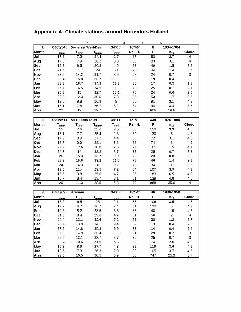
Appendix A: Climate stations around Hottentots Holland
1 2 3 4 5 6
1 0005/545 Somerset West-Dyn 34°05' 18°49' 8 1934-1984Month Tdmax Tdmin Tmmax Tmmin Rel. H. P n10 Cloud.Jul 17.3 7.2 24.4 2.7 87 83 2.7 4Aug 17.6 7.9 26.2 3.3 85 83 3.1 4Sep 19.3 9.5 26.8 4.5 82 49 1.5 3.8Oct 21.4 11.7 29 6.1 76 44 1.4 3.7Nov 23.9 14.2 31.7 8.6 68 24 0.7 3Dec 25.4 15.8 33.7 10.5 66 19 0.4 2.5Jan 26.5 16.7 34.8 11.5 69 17 0.3 1.6Feb 26.7 16.5 34.5 11.9 73 25 0.7 2.1Mar 25.3 15 32.7 10.1 78 24 0.6 2.8Apr 22.5 12.3 30.5 7.3 85 53 1.7 3.6May 19.6 9.8 26.9 5 85 91 3.1 4.3Jun 18.1 7.8 25.7 3.2 84 94 3.4 3.5Ann 22 12 29.7 7 78 606 19.6 3.2
2 0005/611 Steenbras Dam 34°11' 18°51' 339 1926-1960Month Tdmax Tdmin Tmmax Tmmin Rel. H. P n10 Cloud.Jul 15 7.6 22.6 2.5 83 118 3.9 4.6Aug 15.1 7.7 25.4 2.8 82 130 5 4.7Sep 17.2 8.9 27.2 4.4 80 72 3.1 4.6Oct 18.7 9.9 28.1 5.3 78 74 3 4.2Nov 22.2 12.6 30.8 7.5 74 37 1.5 4.1Dec 24.7 14 32.2 8.7 72 25 0.7 3.2Jan 26 15.3 33.7 9.9 72 23 0.8 2.6Feb 25.8 15.6 33.2 11.2 75 46 1.4 3.1Mar 24 14.3 31 9.2 79 34 1 3.3Apr 19.5 11.4 29.5 7.2 84 107 3.9 4.2May 16.5 9.8 25.6 4.7 85 183 6.5 4.8Jun 15.7 8.4 23.7 3.1 81 139 4.8 4.6Ann 20 11.3 28.5 6.3 79 988 35.6 4
3 0005/635 Bizweni 34°05' 18°52' 46 1930-1959Month Tdmax Tdmin Tmmax Tmmin Rel. H. P n10 Cloud.Jul 17.2 6.5 25 2.1 87 106 3.5 4.3Aug 17.7 6.7 26.7 2.4 81 120 5 4.3Sep 19.6 8.2 28.5 3.6 83 48 1.5 4.3Oct 21.3 9.4 29.6 4.7 81 56 2 4Nov 24.4 12.1 32.6 7.2 73 38 1.2 3.7Dec 26.4 13.9 34.1 9.4 69 13 0.4 2.6Jan 27.9 14.8 35.3 9.9 73 14 0.4 2.4Feb 27.9 14.9 35.4 10.3 81 29 0.7 3Mar 26.6 13.1 33.7 8.7 76 25 0.7 3Apr 22.4 10.4 31.5 6.3 89 74 2.6 4.2May 19.8 8.9 27.7 4.3 85 119 3.6 4.6Jun 18.5 7.3 26.3 2.9 83 105 3.7 4.5Ann 22.5 10.5 30.5 5.9 80 747 25.3 3.7
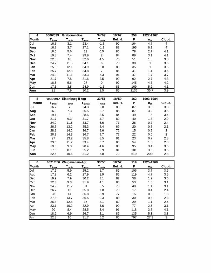
4 0006/039 Grabouw-Bos 34°09' 19°02' 258 1927-1967Month Tdmax Tdmin Tmmax Tmmin Rel. H. P n10 Cloud.Jul 16.5 3.1 23.4 -1.3 90 164 4.7 4Aug 16.8 3.7 27.1 -1.1 88 195 6.1 4Sep 18.6 5.6 29 0.5 86 78 2.7 4.1Oct 19.8 7.4 29.9 2 84 89 3.1 4.1Nov 22.8 10 32.6 4.5 76 51 1.6 3.8Dec 24.7 11.5 34.1 6 78 30 1 3.6Jan 25.8 12.1 34.9 6.8 80 35 1 3.5Feb 25.7 12.8 34.8 7 86 41 1.4 3.6Mar 24.3 11.1 33.3 5.3 91 47 1.7 3.7Apr 21.7 7.8 31.6 2.5 90 92 2.7 4.3May 18.8 5.6 27 0 90 145 4.5 4.2Jun 17.3 3.8 24.9 -1.5 85 169 5.2 4.1Ann 21 7.9 30.2 2.5 85 1136 35.7 3.9
5 0021/591A Elsenburg II Agr 33°51' 18°50' 162 1903-1984Month Tdmax Tdmin Tmmax Tmmin Rel. H. P n10 Cloud.
Jul 16.7 7 24.3 2.8 83 87 3.3 3.3Aug 16.9 7.3 25.5 2.7 85 87 3.2 3.5Sep 19.1 8 28.6 3.5 84 49 1.5 3.4Oct 21.7 9.3 31.7 4.7 80 40 1.3 2.9Nov 24.9 11.6 33.7 6.6 71 26 0.7 2.4Dec 26.6 13.2 35.3 8.4 69 20 0.5 2.1Jan 28.1 14.2 36.7 9.6 72 15 0.2 2Feb 28.3 14.3 36.7 9.7 77 22 0.6 2Mar 27 13.2 35.8 8.5 81 23 0.7 2.3Apr 23.6 11.2 33.4 6.7 83 54 1.8 2.8May 19.5 9.3 28.4 4.6 83 95 3.4 3.5Jun 17.6 8.1 25.2 2.9 81 101 3.6 3.5Ann 22.5 10.6 31.2 5.8 79 619 20.8 2.8
6 0021/656 Welgevallen-Agr 33°56' 18°52' 119 1925-1968Month Tdmax Tdmin Tmmax Tmmin Rel. H. P n10 Cloud.Jul 17.5 5.9 25.2 1.7 89 106 3.7 3.6Aug 17.9 6.2 27.9 1.9 86 119 4.7 3.5Sep 19.9 7.9 30.2 3.1 87 58 1.9 3.6Oct 22.3 9.3 31.9 4.1 85 53 1.8 3.1Nov 24.9 11.7 34 6.5 78 40 1.1 3.1Dec 26.7 13 35.8 7.8 73 17 0.4 2.4Jan 28 14 36.8 8.9 77 15 0.3 1.8Feb 27.8 13.7 36.5 9.3 83 30 0.6 2.3Mar 26.8 12.8 35 8.1 89 29 1.1 2.5Apr 23.1 10.2 32.9 5.6 90 77 2.6 3.1May 20 8.4 28.5 3.4 91 118 3.8 4.1Jun 18.2 6.9 26.7 2.1 87 135 5.3 3.3Ann 22.8 10 31.7 5.2 85 797 27.3 3
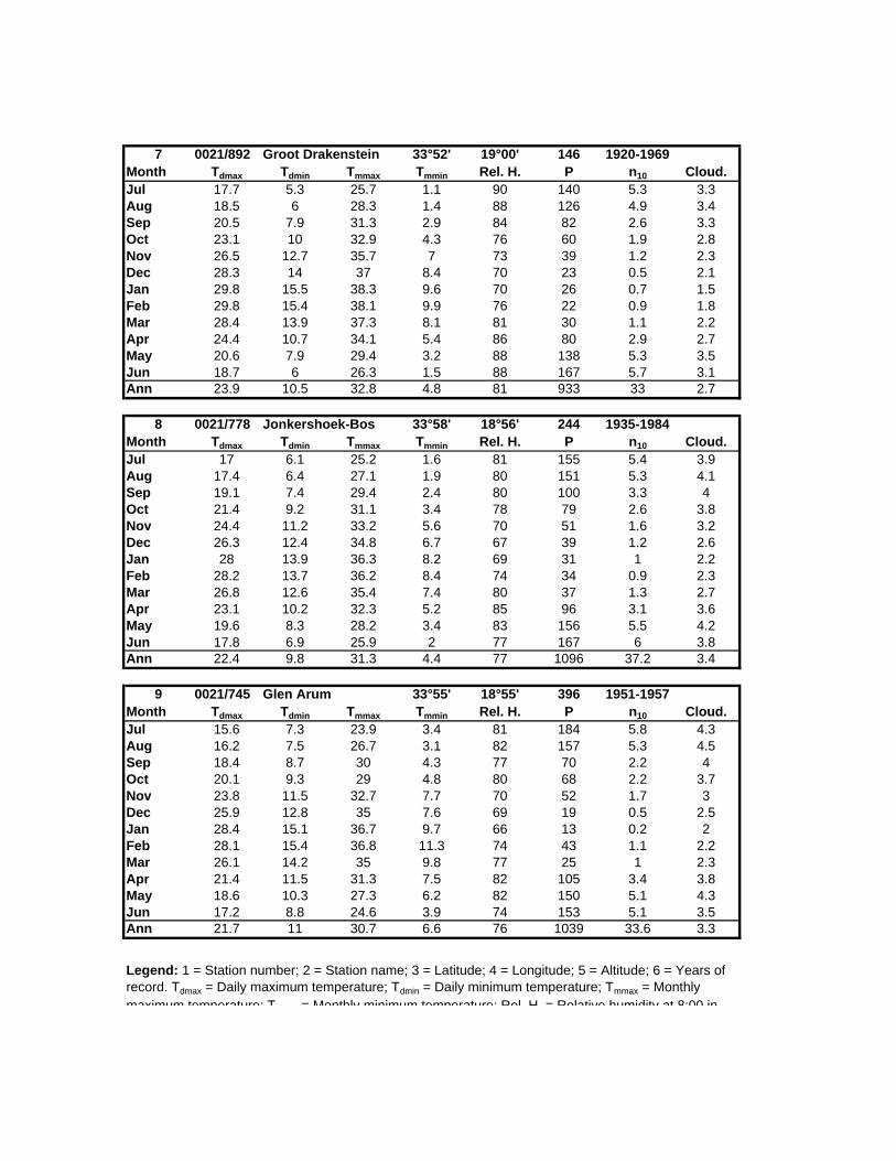
7 0021/892 Groot Drakenstein 33°52' 19°00' 146 1920-1969Month Tdmax Tdmin Tmmax Tmmin Rel. H. P n10 Cloud.Jul 17.7 5.3 25.7 1.1 90 140 5.3 3.3Aug 18.5 6 28.3 1.4 88 126 4.9 3.4Sep 20.5 7.9 31.3 2.9 84 82 2.6 3.3Oct 23.1 10 32.9 4.3 76 60 1.9 2.8Nov 26.5 12.7 35.7 7 73 39 1.2 2.3Dec 28.3 14 37 8.4 70 23 0.5 2.1Jan 29.8 15.5 38.3 9.6 70 26 0.7 1.5Feb 29.8 15.4 38.1 9.9 76 22 0.9 1.8Mar 28.4 13.9 37.3 8.1 81 30 1.1 2.2Apr 24.4 10.7 34.1 5.4 86 80 2.9 2.7May 20.6 7.9 29.4 3.2 88 138 5.3 3.5Jun 18.7 6 26.3 1.5 88 167 5.7 3.1Ann 23.9 10.5 32.8 4.8 81 933 33 2.7
8 0021/778 Jonkershoek-Bos 33°58' 18°56' 244 1935-1984Month Tdmax Tdmin Tmmax Tmmin Rel. H. P n10 Cloud.Jul 17 6.1 25.2 1.6 81 155 5.4 3.9Aug 17.4 6.4 27.1 1.9 80 151 5.3 4.1Sep 19.1 7.4 29.4 2.4 80 100 3.3 4Oct 21.4 9.2 31.1 3.4 78 79 2.6 3.8Nov 24.4 11.2 33.2 5.6 70 51 1.6 3.2Dec 26.3 12.4 34.8 6.7 67 39 1.2 2.6Jan 28 13.9 36.3 8.2 69 31 1 2.2Feb 28.2 13.7 36.2 8.4 74 34 0.9 2.3Mar 26.8 12.6 35.4 7.4 80 37 1.3 2.7Apr 23.1 10.2 32.3 5.2 85 96 3.1 3.6May 19.6 8.3 28.2 3.4 83 156 5.5 4.2Jun 17.8 6.9 25.9 2 77 167 6 3.8Ann 22.4 9.8 31.3 4.4 77 1096 37.2 3.4
9 0021/745 Glen Arum 33°55' 18°55' 396 1951-1957Month Tdmax Tdmin Tmmax Tmmin Rel. H. P n10 Cloud.Jul 15.6 7.3 23.9 3.4 81 184 5.8 4.3Aug 16.2 7.5 26.7 3.1 82 157 5.3 4.5Sep 18.4 8.7 30 4.3 77 70 2.2 4Oct 20.1 9.3 29 4.8 80 68 2.2 3.7Nov 23.8 11.5 32.7 7.7 70 52 1.7 3Dec 25.9 12.8 35 7.6 69 19 0.5 2.5Jan 28.4 15.1 36.7 9.7 66 13 0.2 2Feb 28.1 15.4 36.8 11.3 74 43 1.1 2.2Mar 26.1 14.2 35 9.8 77 25 1 2.3Apr 21.4 11.5 31.3 7.5 82 105 3.4 3.8May 18.6 10.3 27.3 6.2 82 150 5.1 4.3Jun 17.2 8.8 24.6 3.9 74 153 5.1 3.5Ann 21.7 11 30.7 6.6 76 1039 33.6 3.3
Legend: 1 = Station number; 2 = Station name; 3 = Latitude; 4 = Longitude; 5 = Altitude; 6 = Years of record. Tdmax = Daily maximum temperature; Tdmin = Daily minimum temperature; Tmmax = Monthly maximum temperature; T = Monthly minimum temperature; Rel H = Relative humidity at 8:00 in

maximum temperature; Tmmin = Monthly minimum temperature; Rel. H. = Relative humidity at 8:00 in the morning; P = average precipitation; n10 = average number of days with more than 10 mm of rainfall; Cloud. = Cloudiness measured in a scale from 1-8 at 8:00 in the morning
Appendix B: water quality variables Temperature: Temperature is a system variable that regulates many processes such as spawning and migration.
The organisms in the river are adapted to the natural variations in water temperature that occur in diel and seasonal cycles. Disruptions of these natural temperature cycles may have severe impacts on ecosystem functioning and may be caused by thermal pollution, discharge of water from impoundments and removal of riparian vegetation cover.
Dissolved oxygen: The concentrations of dissolved oxygen (DO) are critical for the survival of aquatic organisms
because all organisms use oxygen for their respiration. There is a natural diel cycle in DO-concentrations because of photosynthesis by aquatic plants during the day. In the natural situation, DO-concentrations are often close to saturation. Organic wastes and suspended material will decrease the DO-concentration. This may also increase the effect of toxic waste if present.
pH: pH is a steering variable for many physical and chemical processes. For example, acidification
will mobilize aluminium, which is potentially lethal to aquatic organisms. Natural variations in pH occur in response to diel and seasonal cycles. In the Western Cape pH is likely to be lowest in winter, highest in summer and most variable in autumn. pH can fluctuate as much as one pH unit during a day. In rivers flowing through Mountain Fynbos, the water tends to be acidic because of humic substances that are present in the plant material.
Conductivity and Total Dissolved Solids: Conductivity (EC) refers to the ability of water to conduct an electrical current. This ability is the
result of ions present in the water such as carbonate, sulphate, chloride, sodium etc., all of which carry an electrical charge. TDS (Total Dissolved Solids) is a measure of all dissolved salts in the water. EC and TDS are often positively correlated, although TDS also includes organic compounds that do not carry an electrical charge. Both EC and TDS are dependent on the geological formations, that the water flows through and vary regionally. In the Western Cape EC and TDS tend to be lowest in winter, highest in summer and most variable in autumn.
Turbidity and Total Suspended Solids: Turbidity is a measure of the clarity of the water and TSS (Total Suspended Solids) concentration
is a measure of the amount of material suspended in the water. They are positively correlated. TSS concentrations increase when there is a high sediment load in the river. Anthropogenic factors that influence TSS are agriculture, removal of riparian vegetation and afforestation.
Nutrients: Nutrients such as nitrate, nitrite, ammonia and phosphate are required for plant growth. They
normally occur in low concentrations in the river. Some of them, like nitrite and ammonia, are toxic when they occur in higher concentrations. Toxicity of ammonia will increase with temperature and pH. In South Africa, the principle nutrient controlling eutrophication of aquatic ecosystems is phosphorus. This nutrient, together with inorganic nitrogen has a stimulatory effect on the growth of algae. Eutrophication can occur as a point-source, such as industrial and domestic effluents, or as a diffuse source, such as agricultural runoff (Dallas 1998).
Species name Herbarium codes Notes Synonym (Bond & Goldblatt 1984)LYCOPODIACEAELycopodiella caroliniana (L.) Pic. Serm ES 54 Lycopodium carolinianum L.Lycopodium clavatum L. ES 888
OSMUNDACEAETodea barbara (L.) T.Moore ES 121, ES 378
ANEMIACEAEMohria caffrorum (L.) Desv. ES 301
SCHIZAEACEAESchizaea pectinata (L.) Sw. ES 104Schizaea tenella Kaulf. ES 29
GLEICHENIACEAEGleichenia polypodioides (L.) Sm. ES 222
HYMENOPHYLLACEAESphaerocionium aeruginosum (Poir.) Pic.Serm.
ES 650 Hymenophyllum marlothii Brause
Hymenophyllum peltatum (Poir.) Desv. ES 275
CYATHEACEAECyathea capensis (L.f.) Sm. ES 653, ES 655
DENNSTAEDTIACEAEHistiopteris incisa (Thunb.) J.Sm. ES 566Hypolepis sparsisora (Schrad.) Kuhn ES 563Pteridium aquilinum (L.) Kuhn ES 126
PTERIDACEAEPellaea pteroides (L.) Prantl ES 188
ASPLENIACEAEAsplenium aethiopicum (Burm.f.) Bech. ES 278, ES 391, ES 196
THELYPTERIDACEAEThelypteris confluens (Thunb.) Morton ES 733
LOMARIOPSIDACEAEElaphoglossum angustatum (Schrad.) Hieron.
ES 541
Elaphoglossum conforme (Sw.) J.Sm. ES 342
BLECHNACEAEBlechnum capense Burm.f. ES 129, ES 238Blechnum punctulatum Sw. ES 270, ES 298, ES 347,
ES 572Blechnum punctulatum Sw. ES 651, ES 663 Blechnum attenuatum (Sw.) Mett.Blechnum tabulare (Thunb.) Kuhn ES 633
PODOCARPACEAEPodocarpus cf. elongatus (Aiton) L'Her. ex Pers.
ES 816
(Notes: * = exotic species, O = only recorded outside Hottentots Holland Mountains, -- = only recorded in discarded releve)
Appendix C: Species list
Podocarpus latifolius (Thunb.) R.Br. ex Mirb.
ES 666, ES 816A
PINACEAEPinus cf. pinaster Aiton ES 738 *
CUPRESSACEAEWiddringtonia nodiflora (L.) Powrie ES 77
LAURACEAECassytha ciliolata Nees ES 25
CYPERACEAECarpha glomerata (Thunb.) Nees ES 147, ES 472, ES 252Cyperus denudatus L.f. ES 588Cyperus fastigiatus Rottb. ES 818Ficinia acuminata (Nees) Nees ES 310, ES 467, ES 528,
ES 677Ficinia cf. acuminata (Nees) Nees ES 897 O Ficinia involuta NeesFicinia argyropa Nees ES 867, ES 869Ficinia brevifolia Nees ex Kunth ES 186, ES 700, ES 756Ficinia distans C.B.Clarke ES 561, ES 577, ES 669Ficinia oligantha (Steud.) J.Raynal ES 312, ES 439 Ficinia filiformis (Lam.) Schrad. (ES
439)Ficinia nigrescens (Schrad.) J.Raynal ES 424, ES 478, ES 507Ficinia ramosissima Kunth ES 459Ficinia trichodes (Schrad.) Benth. & Hook.f.
ES 137, ES 235, ES 490
Ficinia species 1 ES 366Ficinia species 2 ES 872Isolepis digitata Schrad. ES 711Isolepis fluitans (L.) R.Br. ES 691, ES 854Isolepis prolifer R.Br. ES 679Epischoenus complanatus Levyns ES 632Epischoenus quadrangularis (Boeck.) C.B.Clarke
ES 775
Epischoenus villosus Levyns ES 451, ES 866, ES 868Epischoenus gracilis Levyns ES 910 OCyathocoma hexandrum (Nees) J. Browning
ES 919 O Macrochaetium hexandrum (Nees) Pfeiffer
Capeobolus brevicaulis (C.B.Clarke) J.Browning
ES 90 Tetraria brevicaulis C.B.Clarke
Tetraria bolusii C.B.Clarke ES 217Tetraria bromoides (Lam.) Pfeiff. ES 477Tetraria capillacea (Thunb.) C.B.Clarke ES 395, ES 434Tetraria crassa Levyns ES 612Tetraria cuspidata (Rottb.) C.B.Clarke ES 102Tetraria fasciata (Rottb.) C.B.Clarke ES 849Tetraria pillansii Levyns ES 611, ES 828Tetraria thermalis (L.) C.B.Clarke ES 609Neesenbeckia punctoria (Vahl) Levyns ES 45Chrysithrix capensis L. ES 108Chrysithrix dodii C.B.Clarke ES 453Chrysithrix junciformis Nees ES 457Schoenoxiphium lanceum (Thunb.) Kük. ES 253, ES 273, ES 285,
ES 383, ES 508Cyperaceae species 1 ES 175, ES 210, ES 846Cyperaceae species 2 ES 534Cyperaceae species 3 ES 669
ARACEAE
Zantedeschia aethiopica (L.) Spreng. ES 499
RESTIONACEAEStaberoha cernua (L.f.) T.Durand & Schinz
ES 397
Staberoha cf. vaginata (Thunb.) Pillans ES 610, ES 614Ischyrolepis cincinnata (Mast.) H.P.Linder ES 158Ischyrolepis curviramis (Kunth) H.P.Linder ES 863Ischyrolepis gaudichaudiana (Kunth) H.P.Linder
ES 23, ES 359, ES 486, ES 877
Ischyrolepis helenae (Mast.) H.P.Linder ES 793Ischyrolepis subverticillata Steud. ES 41, ES 861Ischyrolepis triflora (Rottb.) H.P.Linder ES 69, ES 791Elegia asperiflora (Nees) Kunth ES 236Elegia capensis (Burm.f.) Schelpe ES 127Elegia grandis (Nees) Kunth ES 830Elegia intermedia (Steud.) Pillans ES 21, ES 543, ES 550,
ES 645Elegia neesii Mast. ES 60Elegia persistens Mast. ES 156Elegia racemosa (Poir.) Pers. ES 630, ES 638, ES 642Elegia spathacea Mast. ES 178, ES 402, ES 706,
ES 792Chondropetalum deustum Rottb. ES 165A, ES 332Chondropetalum ebracteatum (Kunth) Pillans
ES 796
Chondropetalum mucronatum (Nees) Pillans
ES 14, ES 115, ES 163, ES 393
Askidiosperma cf. chartaceum (Pillans) H.P.Linder
ES 319
Askidiosperma esterhuyseniae (Pillans) H.P.Linder
ES 7, ES 9, ES 60A, ES 62, ES 98, ES 160
Platycaulos callistachyus (Kunth) H.P.Linder
ES 135, ES 859
Platycaulos cascadensis (Pillans) H.P.Linder
ES 785
Platycaulos depauperatus (Kunth) H.P.Linder
ES 644, ES 742
Restio ambiguus Mast. ES 926 O Restio bifarius Mast. ES 320Restio bifidus Thunb. ES 52, ES 874 Restio bifurcus Nees ex Mast. ES 827Restio burchellii Pillans ES 161, ES 790, ES 848Restio brachiatus (Mast.) Pillans ES 909 O Restio corneolus Esterh. ES 322, ES 400Restio debilis Nees ES 420 Restio intermedius (Pillans) H.P.Linder ES 326, ES 463, ES 548,
ES 780Restio degenerans Pillans
Restio dispar Mast. ES 843Restio echinatus Kunth ES 165Restio egregius Hochst. ES 850, ES 851Restio ejuncidus Mast. ES 604Restio filiformis Poir. ES 533Restio nuwebergensis Esterh. ES 431Restio obscurus Pillans ES 916 O Restio occultus (Mast.) Pillans ES 154Restio cf. pedicellatus Mast. ES 902, ES 912 O Restio cf. perplexus Kunth ES 66, ES 724, ES 881Restio purpurascens Nees ex Mast. ES 22, ES 101Restio quadratus Mast. ES 247Restio stokoei Pillans ES 799
Restio subtilis Nees ex Mast. ES 450Restio af. versatilis H.P.Linder ES 456, ES 605, ES 615Calopsis paniculata (Rottb.) Desv. ES 357Calopsis hyalina (Mast.) H.P.Linder ES 934 O Thamnochortus fruticosus P.J.Bergius ES 436, ES 489Thamnochortus lucens (Poir.) H.P.Linder ES 428, ES 804Ceratocaryum argenteum Nees ex Kunth ES 115A, ES 323Cannomois virgata (Rottb.) Steud. ES 140, ES 209Nevillea obtusissima (Steud.) H.P.Linder ES 42Anthochortus crinalis (Mast.) H.P.Linder ES 452, ES 637, ES 826,
ES 865Anthochortus ecklonii Nees ES 864Anthochortus cf. graminifolius (Kunth) H.P.Linder
ES 832
Anthochortus laxiflorus (Nees) H.P.Linder ES 30, ES 784Mastersiella digitata (Thunb.) Gilg-Ben. ES 852Hypodiscus aristatus (Thunb.) Krauss ES 620Willdenowia sulcata Mast. ES 789
PRIONIACEAEPrionium serratum (L.f.) Drege ex E.Mey. ES 152, ES 875
JUNCACEAEJuncus capensis Thunb. ES 681Juncus cephalotes Thunb. ES 684Juncus effusus L. ES 701Juncus lomatophyllus Spreng. ES 245, ES 340
POACEAECymbopogon cf. marginatus (Steud.) Stapf ex Burtt Davy
ES 502
Themeda triandra Forssk. ES 491, ES 765Paspalum urvillei Steud. ES 687, ES 730, ES 823 *Panicum maximum Jacq. ES 723Ehrharta erecta Lam. ES 132, ES 388, ES 597Ehrharta rehmannii Stapf ES 74, ES 597 Ehrharta setacea Nees subsp. setacea ES 454Ehrharta setacea Nees subsp. uniflora (Burch. ex Stapf) Gibbs-Russ.
ES 465, ES 547, ES 551
Ehrharta ramosa ES 906 OAnthoxanthum tongo (Trin.) Stapf ES 524, ES 559, ES 702Pennisetum macrourum Trin. ES 679Pentaschistis ampla (Nees) McClean ES 240, ES 761Pentaschistis curvifolia (Schrad.) Stapf ES 112Pentaschistis densifolia (Nees) Stapf ES 688Pentaschistis holciformis (Nees) H.P.Linder
ES 430, ES 853
Pentaschistis malouinensis (Steud.) Clayton
ES 88, ES 720, ES 885
Pentaschistis pallida (Thunb.) H.P.Linder ES 333, ES 337, ES 530, ES 668, ES 716
Pentameris distichophylla (Lehm.) Nees ES 734Pentameris hirtiglumis N.P.Barker ES 628, ES 629Pentameris macrocalycina (Steud.) Schweick.
ES 416
Pentameris thuarii P.Beauv. ES 206, ES 464, ES 479Pseudopentameris obtusifolia (Hochst.) N.P. Barker
ES 857 Pentameris obtusifolia (Hochst.) Schweick.
Agrostis cf. avenacea C.C.Gmel. ES 735 *Eragrostis curvula (Schrad.) Nees ES 300
Tribolium cf. brachystachyum (Nees) Renvoize
ES 241, ES 699
Merxmuellera stricta (Schrad.) Conert ES 933 OBriza maxima L. ES 696 *
HYACINTHACEAEAlbuca echinosperma U. Mull.-Doblies ES 891
HEMEROCALLIDACEAECaesia contorta (L.f.) T.Durand & Schinz ES 578
ASPHODELACEAEBulbine cepacea (Burm.f.) Wijnands ES 671 Bulbine tuberosa (Mill.) Oberm.Bulbine species ES 503Bulbinella nutans (Thunb.) T.Durand & Schinz
ES 907 O
Trachyandra hirsuta (Thunb.) Kunth ES 511Trachyandra tabularis (Baker) Oberm. ES 678Kniphofia tabularis Marloth ES 552Aloe mitriformis Mill. ES 380Aloe plicatilis (L.) Mill. ES 510Asphodelaceae species ES 355
ASPARAGACEAEAsparagus retrofractus L. ES 469 Protasparagus retrofractus (L.)
Oberm.Asparagus rubicundus P.J. Bergius ES 486 Protasparagus rubicundus
(P.J.Bergius) Oberm.Asparagus scandens Thunb. ES 518 Myrsiphyllum scandens (Thunb.)
Oberm.Asparagus volubilis Thunb. ES 570 Myrsiphyllum volubile (Thunb.)
Oberm.
TECOPHILAEACEAECyanella species ES 501
HAEMODORACEAEDilatris viscosa L.f. ES 800Wachendorfia brachyandra W.F.Barker ES 665Wachendorfia thyrsiflora Burm. ES 725
IRIDACEAEMoraea collina Thunb. ES 476 Homeria collina (Thunb.) Salisb.Bobartia gladiata (L.f.) Ker Gawl. ES 174Bobartia indica L. ES 216Aristea cf. africana (L.) Hoffmanns. ES 177Aristea bakeri Klatt ES 133, ES 190, ES 414,
ES 488Aristea confusa Goldblatt
Aristea latifolia G.J.Lewis ES 652Aristea major Andrews ES 68, ES 110, ES 233,
ES 352Geissorhiza ovalifolia R.C.Foster ES 522 Geissorhiza umbrosa G.J.Lewis ES 617 Geissorhiza species 1 ES 656Geissorhiza species 2 ES 795Chasmanthe aethiopica (L.) N.E.Br. ES 354Gladiolus carneus D.Delaroche ES 667, ES 787, ES 795Gladiolus species ES 93Tritoniopsis dodii (G.J.Lewis) G.J.Lewis ES 421Tritoniopsis lata (L.Bolus) G.J.Lewis ES 78Watsonia borbonica (Pourr.) Goldblatt ES 664
Watsonia schlechteri L.Bolus ES 855Iridaceae species1 ES 151Iridaceae species 2 ES 466Iridaceae species 3 ES 659
ORCHIDACEAE Holothrix villosa Lindl. ES 427, ES 538 Disa tripetaloides (L.f.) N.E.Br. ES 717 Orchidaceae species 1 ES 345Orchidaceae species 2 ES 515Orchidaceae species 3 ES 782
MYRICACEAEMorella serrata (Lam.) Killick ES 686 Myrica serrata Lam.
PROTEACEAEBrabejum stellatifolium L. ES 50, ES 141Protea amplexicaulis (Salisb.) R.Br. ES 884Protea cynaroides (L.) L. ES 65Protea grandiceps Tratt. ES 810Protea repens (L.) L. ES 423Protea lacticolor Salisb. ES 422Protea neriifolia R.Br. ES 704Protea nitida Mill. ES 767Leucadendron cf. gandogeri Schinz ex Gand.
ES 412
Leucadendron cf. laureolum (Lam.) Fourc. ES 46, ES 886
Leucadendron microcephalum (Gand.) Gand. & Schinz
ES 809
Leucadendron xanthoconus (Kuntze) K.Schum.
ES 122
Hakea sericea Schrad. ES 847 *
VISCACEAEViscum pauciflorum L.f. ES 381
SANTALACEAEThesium cf. capituliflorum Sond. ES 858Thesium carinatum DC. ES 736Thesium paniculatum L. ES 287Thesium scabrum L. ES 766Thesium cf. spicatum L. ES 751Thesium strictum P.J.Bergius ES 207, ES 309, ES 537Thesium viridifolium Levyns ES 807
GRUBBIACEAEGrubbia rosmarinifolia P.J.Bergius ES 39, ES 448, ES 709
FUMARIACEAEFumaria muralis Sond. ex W.D.J.Koch ES 581 *RANUNCULACEAEKnowltonia capensis (L.) Huth ES 825Knowltonia vesicatoria (L.f.) Sims ES 509
DROSERACEAEDrosera aliciae Raym.-Hamet ES 40Drosera capensis L. ES 707Drosera glabripes (Harv.) Stein ES 719
CRASSULACEAE
Crassula capensis (L.) Baill. ES 519, ES 521 -- Crassula dejecta Jacq. ES 193, ES 758, ES 824Crassula muscosa L. ES 514Crassula nudicaulis L. ES 532Crassula species ES 579
MONTINIACEAEMontinia caryophyllacea Thunb. ES 494
PITTOSPORACEAEPittosporum undulatum Vent. ES 386 *
CUNONIACEAEPlatylophus trifoliatus (L.f.) D.Don ES 148Cunonia capensis L. ES 142
BRUNIACEAERaspalia microphylla (Thunb.) Brongn. ES 783Raspalia virgata (Brongn.) Pillans ES 649Nebelia fragarioides (Willd.) Kuntze ES 401Pseudobaeckea africana (Burm.f.) Pillans ES 4, ES 408Brunia alopecuroides Thunb. ES 12, ES 37A, ES 97Berzelia lanuginosa (L.) Brongn. ES 12A, ES 37Berzelia squarrosa (Thunb.) Sond. ES 11, ES 330, ES 398
ROSACEAERubus cf. pinnatus Willd. ES 361Rubus cf. rigidus Sm. ES 680Cliffortia apiculata Weim. ES 329Cliffortia atrata Weim. ES 70, ES 159, ES 324,
ES 417, ES 441, ES 516Cliffortia complanata E.Mey. ES 520, ES 718, ES 747Cliffortia cuneata Aiton ES 244Cliffortia dodecandra Weim. ES 214, ES 435Cliffortia dregeana C.Presl ES 936 OCliffortia eriocephalina Cham. ES 555 Cliffortia graminea L.f. ES 744Cliffortia grandifolia Eckl. & Zeyh. ES 213Cliffortia hirsuta Eckl. & Zeyh. ES 16Cliffortia integerrima Weim. ES 808Cliffortia odorata L.f. ES 583Cliffortia ovalis Weim. ES 625, ES 802Cliffortia pedunculata Schltr. ES 51Cliffortia polygonifolia L. ES 243, ES 726Cliffortia ruscifolia L. ES 184Cliffortia cf. sericea Eckl. & Zeyh. ES 70ACliffortia strobilifera Murray ES 697Cliffortia tricuspidata Harv. ES 643
FABACEAEAcacia longifolia (Andrews) Willd. ES 737 *Acacia mearnsii De Wild. ES 695 *Acacia saligna (Labill.) H.L.Wendl. ES 146 *Virgilia oroboides (P.J.Bergius) Salter ES 890Cyclopia maculata (Andrews) Kies ES 672, ES 675Podalyria calyptrata (Retz.) Willd. ES 99Podalyria species ES 616 Podalyria montana Hutch.Liparia capitata Thunb. ES 845 Priestleya capitata (Thunb.) DC.Aspalathus ciliaris L. ES 753Aspalathus laricifolia P.J.Bergius ES 497
Argyrolobium lunare (L.) Druce ES 481 Argyrolobium lanceolatum Eckl. & Zeyh.
Hypocalyptus sophoroides (P.J.Bergius) Baill.
ES 560
Psoralea aphylla L. ES 440Psoralea asarina (P.J.Bergius) Salter ES 574Psoralea pinnata L. ES 575Psoralea aculeata L. ES 94Psoralea af. fleta C. H. Stirton ined. ES 134, ES 471Otholobium obliquum (E.Mey.) C.H.Stirt. ES 492, ES 674Tephrosia capensis (Jacq.) Pers. ES 769Bolusafra bituminosa (L.) Kuntze ES 589Dipogon lignosus (L.) Verdc. ES 304Dolichos decumbens Thunb. ES 535
GERANIACEAEPelargonium columbinum Jacq. ES 587Pelargonium cucullatum (L.) L'Hér. ES 284Pelargonium elongatum (Cav.) Salisb. ES 576Pelargonium hermanniifolium (P.J.Bergius) Jacq.
ES 250
Pelargonium patulum Jacq. ES 306, ES 506, ES 844Pelargonium tomentosum Jacq. ES 349
OXALIDACEAEOxalis cf. corniculata L. ES 531 *Oxalis livida Jacq. var. altior ES 272, ES 661 Oxalis dentata Jacq.Oxalis livida Jacq. ES 364Oxalis lanata L.f. ES 365Oxalis cf. nidulans Eckl. & Zeyh. ES 219, ES 317Oxalis purpurea L. ES 363, ES 513Oxalis truncatula Jacq. ES 444, ES 485Oxalis cf. versicolor L. ES 495Oxalis species 1 ES 523Oxalis species 2 ES 882Oxalis species 3 ES 898 O
RUTACEAEAgathosma capensis (L.) Dummer ES 254 Agathosma crenulata (L.) Pillans ES 76, ES 100Agathosma pentachotoma E. Mey. ex Sond.
ES 911 O
Adenandra acuta Schltr. ES 606Coleonema juniperinum Sond. ES 432Diosma cf. hirsuta L. ES 752Diosma thyrsophora Eckl. & Zeyh. ES 806Euchaetis glabra I.Williams ES 829Empleurum unicapsulare (L.f.) Skeels ES 264
POLYGALACEAEPolygala cf. nematocaulis Levyns ES 85, ES 929Muraltia alba Levyns ES 367Muraltia heisteria (L.) DC. ES 205, ES 230Muraltia vulpina Chodat ES 498
EUPHORBIACEAEClutia alaternoides L. ES 586, ES 596Clutia alaternoides L. ES 673, ES 759 Clutia rubricaulis Eckl. ex Sond.Clutia laxa Eckl. ex Sond. ES 316Clutia polygonoides L. ES 237A, ES 607, ES Euphorbia epicyparissias E.Mey. ex Boiss. ES 314
ANACARDIACEAEHeeria argentea (Thunb.) Meisn. ES 764Rhus angustifolia L. ES 251Rhus tomentosa L. ES 351
AQUIFOLIACEAEIlex mitis (L.) Radlk. ES 124, ES 276
CELASTRACEAEMaytenus acuminata (L.f.) Loes. ES 387Maytenus oleoides (Lam.) Loes. ES 390Pterocelastrus rostratus Walp. ES 569Cassine schinoides (Spreng.) R.H. Archer ES 189, ES 255 Hartogiella schinoides (Spreng.)
ICACINACEAEApodytes dimidiata E.Mey. ex Arn. ES 338, ES 343, ES 539
RHAMNACEAEPhylica callosa L.f. ES 836Phylica ericoides L. ES 425, ES 860Phylica gracilis (Eckl. & Zeyh.) D.Dietr. ES 237Phylica imberbis P.J.Bergius ES 760, ES 862Phylica plumosa L. ES 705 Phylica pubescens Aiton ES 286, ES 288Phylica strigulosa Sond. ES 880
MALVACEAEHibiscus trionum L. ES 595 *Hermannia alnifolia L. ES 585
KIGGELARIACEAEKiggelaria africana L. ES 277, ES 382, ES 389,
ES 564
PENAEACEAEPenaea cneorum Meerb. ES 712Penaea mucronata L. ES 221
OLINIACEAEOlinia ventosa (L.) Cufod. ES 814
THYMELAEACEAEGnidia cf. anomala Meisn. ES 229Gnidia galpinii C.H.Wright ES 608, ES 774, ES 803Gnidia oppositifolia L. ES 413Struthiola ciliata (L.) Lam. ES 212Struthiola martiana Meisn. ES 721, ES 797Struthiola myrsinites Lam. ES 394Passerina vulgaris Thoday ES 728
MYRTACEAEMetrosideros angustifolia (L.) Sm. ES 125
HALORAGACEAELaurembergia repens P.J.Bergius subsp. brachypoda (Hiern) Oberm.
ES 727
ARALIACEAECentella caespitosa Adamson ES 618
Centella difformis (Eckl. & Zeyh.) Adamson
ES 776
Centella eriantha (A.Rich.) Drude ES 73, ES 249, ES 292 Centella af. laevis AdamsonCentella macrocarpa (Rich.) Adamson ES 438Centella montana (Cham. & Schltdl.) Domin
ES 291, ES 487
APIACEAELichtensteinia lacera Cham. & Schltdl. ES 493Glia prolifera (Burm.f.) B.L.Burtt ES 376, ES 839Hermas species ES 805Peucedanum galbaniopse H.Wolff ES 703Peucedanum galbanum (L.) Drude ES 182Peucedanum cf. strictum (Spreng.) B.L.Burtt
ES 475
CORNACEAECurtisia dentata (Burm.f.) C.A.Sm. ES 811
ERICACEAEErica autumnalis L.Bolus ES 613, ES 631, ES 647 Erica caffra L. ES 470Erica calycina L. ES 602Erica coccinea L. ES 600Erica corifolia L. ES 859Erica curviflora L. ES 741Erica curvirostris Salisb. ES 80, ES 106, ES 187Erica fastigiata L. ES 601Erica hispidula L. ES 59, ES 82, ES 407,
ES 545Erica imbricata L. ES 437Erica intervallaris Salisb. ES 409, ES 449, ES 621Erica longifolia Aiton ES 418Erica lucida Salisb. ES 473Erica lutea P.J.Bergius ES 117Erica nudiflora L. ES 223Erica equisetifolia Salisb. ES 48, ES 81, ES 399,
ES 777Blaeria equisetifolia (Salisb.) G.Don.
Erica pinea Thunb. ES 842Erica plukenetii L. ES 621AErica sessiliflora L.f. ES 107Erica sitiens Klotzsch ES 603, ES 773Erica hirta Thunb. ES 295 Erica sphaeroidea DulferErica strigosa Sol. ES 750Erica tegulifolia Salisb. ES 181Erica triflora L. ES 259, ES 646Erica labialis Salisb. ES 31 Sympieza labialis (Salisb.) DruceErica artemisioides (Klotzsch) E.G.H. Oliv. ES 749, ES 879 Scyphogyne micrantha (Benth.)
N.E.Br.Erica species ES 265
MYRSINACEAEMyrsine africana L. ES 303, ES 512Rapanea melanophloeos (L.) Mez ES 540
EBENACEAEDiospyros glabra (L.) De Winter ES 200, ES 263, ES 296Diospyros whyteana (Hiern) F.White ES 813
OLEACEAEOlea capensis L. ES 544, ES 812
Olea europaea L. subsp. africana (Mill.) P.S.Green
ES 662
GENTIANACEAEChironia baccifera L. ES 368, ES 755Chironia jasminoides L. ES 109 Chironia decumbens ES 923
MENYANTHACEAEVillarsia capensis (Houtt.) Merr. ES 33
APOCYNACEAESecamone alpini Schult. ES 754
CONVOLVULACEAECuscuta nitida E. Mey. ex Choisy ES 713
STILBACEAEKogelbergia verticillata (Eckl. & Zeyh.) Rourke
ES 339 Stilbe mucronata N.E.Br.
LAMIACEAELeonotis leonurus (L.) R.Br. ES 591Stachys aethiopica L. ES 593Salvia chamelaeagnea P.J.Bergius ES 350
SOLANACEAESolanum retroflexum Dunal ES 567
SCROPHULARIACEAEHemimeris racemosa (Houtt.) Merrill ES 584 Hemimeris montana L.f.Halleria elliptica Thunb. ES 282Halleria lucida L. ES 546Oftia africana (L.) Bocq. ES 474Sutera hispida (Thunb.) Druce ES 358Pseudoselago serrata (P.J. Bergius) ES 290, ES 370, ES 817 Selago serrata P.J.BergiusMicrodon dubius (L.) Hilliard ES 771 Agathelpis dubia (L.) Hutch.
RUBIACEAEAnthospermum cf. aethiopicum L. ES 729Anthospermum galioides Rchb.f. ES 232, ES 429Anthospermum cf. spathulatum Spreng. ES 748Galium tomentosum Thunb. ES 462Carpacoce spermacocea (Rchb.f.) Sond. ES 75, ES 403
LENTIBULARIACEAEUtricularia bisquamata Schrank ES 622, ES 710
CAMPANULACEAERoella dregeana A.DC. ES 779Wahlenbergia procumbens (Thunb.) A.DC.
ES 798, ES 831
Wahlenbergia parvifolia (P.J. Bergius) Lammers
ES 283 Lightfootia parvifolia (P.J.Bergius) Adamson
Cyphia volubilis (Burm.f.) Willd. ES 372, ES 484, ES 590Lobelia erinus L. ES 580Lobelia jasionoides (A.DC.) E.Wimm. ES 639Monopsis lutea (L.) Urb. ES 683Wimmerella bifida (Thunb.) L. Serra, M.B. Crespo & Lammers
ES 682 Laurentia arabidea (C.Presl) A.DC.
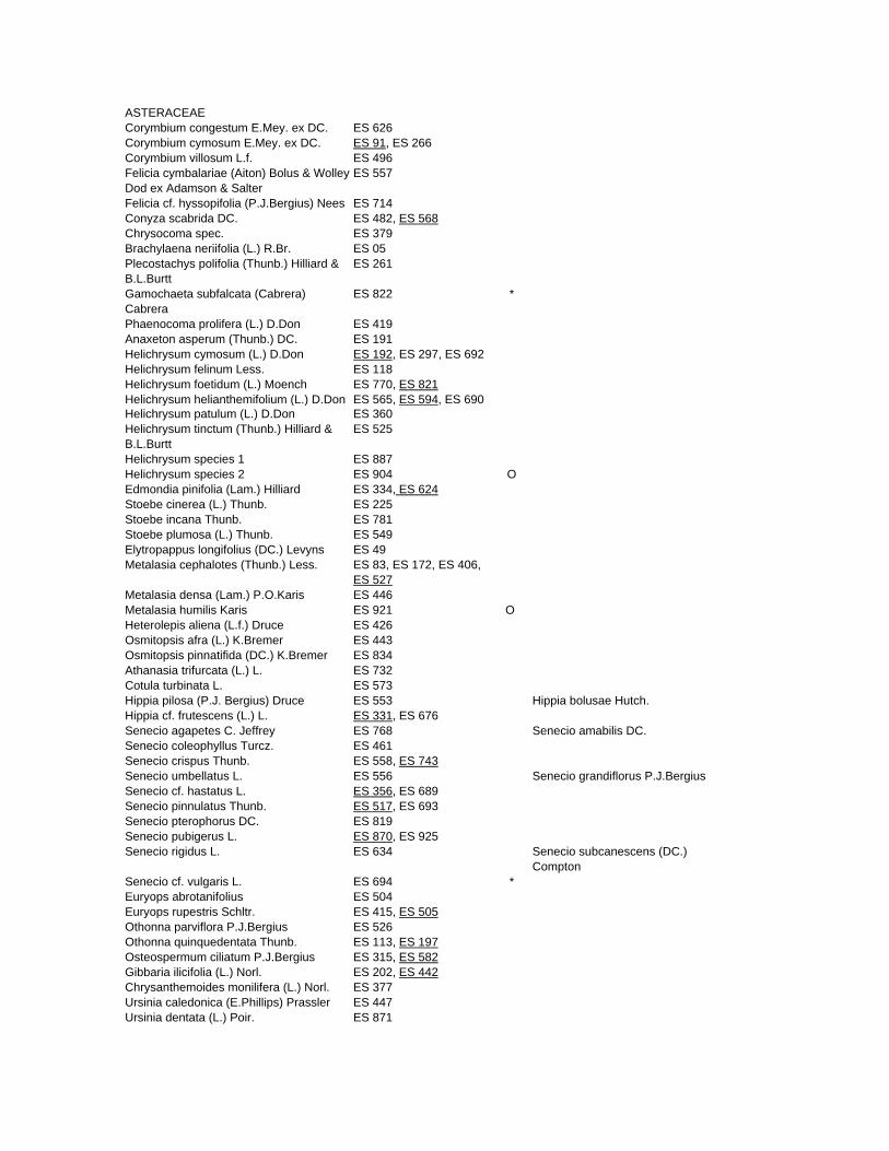
ASTERACEAECorymbium congestum E.Mey. ex DC. ES 626Corymbium cymosum E.Mey. ex DC. ES 91, ES 266Corymbium villosum L.f. ES 496Felicia cymbalariae (Aiton) Bolus & Wolley-Dod ex Adamson & Salter
ES 557
Felicia cf. hyssopifolia (P.J.Bergius) Nees ES 714Conyza scabrida DC. ES 482, ES 568Chrysocoma spec. ES 379Brachylaena neriifolia (L.) R.Br. ES 05Plecostachys polifolia (Thunb.) Hilliard & B.L.Burtt
ES 261
Gamochaeta subfalcata (Cabrera) Cabrera
ES 822 *
Phaenocoma prolifera (L.) D.Don ES 419Anaxeton asperum (Thunb.) DC. ES 191Helichrysum cymosum (L.) D.Don ES 192, ES 297, ES 692Helichrysum felinum Less. ES 118 Helichrysum foetidum (L.) Moench ES 770, ES 821Helichrysum helianthemifolium (L.) D.Don ES 565, ES 594, ES 690Helichrysum patulum (L.) D.Don ES 360Helichrysum tinctum (Thunb.) Hilliard & B.L.Burtt
ES 525
Helichrysum species 1 ES 887Helichrysum species 2 ES 904 OEdmondia pinifolia (Lam.) Hilliard ES 334, ES 624Stoebe cinerea (L.) Thunb. ES 225 Stoebe incana Thunb. ES 781Stoebe plumosa (L.) Thunb. ES 549Elytropappus longifolius (DC.) Levyns ES 49Metalasia cephalotes (Thunb.) Less. ES 83, ES 172, ES 406,
ES 527Metalasia densa (Lam.) P.O.Karis ES 446Metalasia humilis Karis ES 921 O Heterolepis aliena (L.f.) Druce ES 426Osmitopsis afra (L.) K.Bremer ES 443Osmitopsis pinnatifida (DC.) K.Bremer ES 834Athanasia trifurcata (L.) L. ES 732Cotula turbinata L. ES 573Hippia pilosa (P.J. Bergius) Druce ES 553 Hippia bolusae Hutch.Hippia cf. frutescens (L.) L. ES 331, ES 676Senecio agapetes C. Jeffrey ES 768 Senecio amabilis DC.Senecio coleophyllus Turcz. ES 461Senecio crispus Thunb. ES 558, ES 743Senecio umbellatus L. ES 556 Senecio grandiflorus P.J.BergiusSenecio cf. hastatus L. ES 356, ES 689Senecio pinnulatus Thunb. ES 517, ES 693Senecio pterophorus DC. ES 819Senecio pubigerus L. ES 870, ES 925Senecio rigidus L. ES 634 Senecio subcanescens (DC.)
ComptonSenecio cf. vulgaris L. ES 694 *Euryops abrotanifolius ES 504Euryops rupestris Schltr. ES 415, ES 505Othonna parviflora P.J.Bergius ES 526Othonna quinquedentata Thunb. ES 113, ES 197Osteospermum ciliatum P.J.Bergius ES 315, ES 582Gibbaria ilicifolia (L.) Norl. ES 202, ES 442Chrysanthemoides monilifera (L.) Norl. ES 377Ursinia caledonica (E.Phillips) Prassler ES 447Ursinia dentata (L.) Poir. ES 871
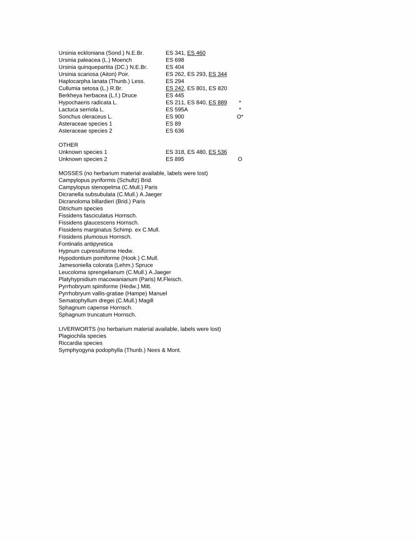
Ursinia eckloniana (Sond.) N.E.Br. ES 341, ES 460Ursinia paleacea (L.) Moench ES 698Ursinia quinquepartita (DC.) N.E.Br. ES 404Ursinia scariosa (Aiton) Poir. ES 262, ES 293, ES 344Haplocarpha lanata (Thunb.) Less. ES 294Cullumia setosa (L.) R.Br. ES 242, ES 801, ES 820Berkheya herbacea (L.f.) Druce ES 445Hypochaeris radicata L. ES 211, ES 840, ES 889 *Lactuca serriola L. ES 595A * Sonchus oleraceus L. ES 900 O*Asteraceae species 1 ES 89 Asteraceae species 2 ES 636
OTHERUnknown species 1 ES 318, ES 480, ES 536Unknown species 2 ES 895 O
Campylopus pyriformis (Schultz) Brid.Campylopus stenopelma (C.Mull.) ParisDicranella subsubulata (C.Mull.) A.JaegerDicranoloma billardieri (Brid.) ParisDitrichum speciesFissidens fasciculatus Hornsch.Fissidens glaucescens Hornsch.Fissidens marginatus Schimp. ex C.Mull.Fissidens plumosus Hornsch.Fontinalis antipyreticaHypnum cupressiforme Hedw.Hypodontium pomiforme (Hook.) C.Mull.Jamesoniella colorata (Lehm.) SpruceLeucoloma sprengelianum (C.Mull.) A.JaegerPlatyhypnidium macowanianum (Paris) M.Fleisch.Pyrrhobryum spiniforme (Hedw.) Mitt.Pyrrhobryum vallis-gratiae (Hampe) ManuelSematophyllum dregei (C.Mull.) MagillSphagnum capense Hornsch.Sphagnum truncatum Hornsch.
Plagiochila speciesRiccardia speciesSymphyogyna podophylla (Thunb.) Nees & Mont.
MOSSES (no herbarium material available, labels were lost)
LIVERWORTS (no herbarium material available, labels were lost)
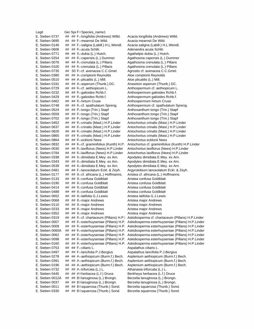
Legit GenSpeF GSpecies_name1 E. Sieben 0737 ## ## F Alongifolia (Andrews) Willd. Acacia longifolia (Andrews) Willd.E. Sieben 0695 ## ## F Amearnsii De Wild. Acacia mearnsii De Wild.E. Sieben 0146 ## ## F Asaligna (Labill.) H.L.Wendl. Acacia saligna (Labill.) H.L.Wendl.E. Sieben 0606 ## ## RAacuta Schltr. Adenandra acuta Schltr.E. Sieben 0771 ## ## SAdubia (L.) Hutch. Agathelpis dubia (L.) Hutch.E. Sieben 0254 ## ## RAcapensis (L.) Dummer Agathosma capensis (L.) DummerE. Sieben 0076 ## ## RAcrenulata (L.) Pillans Agathosma crenulata (L.) PillansE. Sieben 0100 ## ## RAcrenulata (L.) Pillans Agathosma crenulata (L.) PillansE. Sieben 0735 ## 50 PAcf. avenacea C.C.Gmel. Agrostis cf. avenacea C.C.Gmel.E. Sieben 0380 ## ## AAcomptonii Reynolds Aloe comptonii ReynoldsE. Sieben 0510 ## ## AAplicatilis (L.) Mill. Aloe plicatilis (L.) Mill.E. Sieben 0191 ## ## AAasperum (Thunb.) DC. Anaxeton asperum (Thunb.) DC.E. Sieben 0729 ## ## RAcf. aethiopicum L. Anthospermum cf. aethiopicum L.E. Sieben 0232 ## ## RAgalioides Rchb.f. Anthospermum galioides Rchb.f.E. Sieben 0429 ## ## RAgalioides Rchb.f. Anthospermum galioides Rchb.f.E. Sieben 0462 ## ## RAhirtum Cruse Anthospermum hirtum CruseE. Sieben 0748 ## ## RAcf. spathulatum Spreng. Anthospermum cf. spathulatum Spreng.E. Sieben 0524 ## ## PAtongo (Trin.) Stapf Anthoxanthum tongo (Trin.) StapfE. Sieben 0559 ## ## PAtongo (Trin.) Stapf Anthoxanthum tongo (Trin.) StapfE. Sieben 0702 ## ## PAtongo (Trin.) Stapf Anthoxanthum tongo (Trin.) StapfE. Sieben 0452 ## ## RAcrinalis (Mast.) H.P.Linder Antochortus crinalis (Mast.) H.P.LinderE. Sieben 0637 ## ## RAcrinalis (Mast.) H.P.Linder Antochortus crinalis (Mast.) H.P.LinderE. Sieben 0826 ## ## RAcrinalis (Mast.) H.P.Linder Antochortus crinalis (Mast.) H.P.LinderE. Sieben 0865 ## ## RAcrinalis (Mast.) H.P.Linder Antochortus crinalis (Mast.) H.P.LinderE. Sieben 0864 ## ## RAecklonii Nees Antochortus ecklonii NeesE. Sieben 0832 ## ## RAcf. graminifolius (Kunth) H.P.L Antochortus cf. graminifolius (Kunth) H.P.LinderE. Sieben 0030 ## ## RAlaxiflorus (Nees) H.P.Linder Antochortus laxiflorus (Nees) H.P.LinderE. Sieben 0784 ## ## RAlaxiflorus (Nees) H.P.Linder Antochortus laxiflorus (Nees) H.P.LinderE. Sieben 0338 ## ## ICAdimidiata E.Mey. ex Arn. Apodytes dimidiata E.Mey. ex Arn.E. Sieben 0343 ## ## ICAdimidiata E.Mey. ex Arn. Apodytes dimidiata E.Mey. ex Arn.E. Sieben 0539 ## ## ICAdimidiata E.Mey. ex Arn. Apodytes dimidiata E.Mey. ex Arn.E. Sieben 0481 ## ## F Alanceolatum Eckl. & Zeyh. Argyrolobium lanceolatum Eckl. & Zeyh.E. Sieben 0177 ## ## IRAcf. africana (L.) Hoffmanns. Aristea cf. africana (L.) Hoffmanns.E. Sieben 0133 ## ## IRAconfusa Goldblatt Aristea confusa GoldblattE. Sieben 0190 ## ## IRAconfusa Goldblatt Aristea confusa GoldblattE. Sieben 0414 ## ## IRAconfusa Goldblatt Aristea confusa GoldblattE. Sieben 0488 ## ## IRAconfusa Goldblatt Aristea confusa GoldblattE. Sieben 0652 ## ## IRAlatifolia G.J.Lewis Aristea latifolia G.J.LewisE. Sieben 0068 ## ## IRAmajor Andrews Aristea major AndrewsE. Sieben 0110 ## ## IRAmajor Andrews Aristea major AndrewsE. Sieben 0233 ## ## IRAmajor Andrews Aristea major AndrewsE. Sieben 0352 ## ## IRAmajor Andrews Aristea major AndrewsE. Sieben 0319 ## ## RAcf. chartaceum (Pillans) H.P.L Askidiosperma cf. chartaceum (Pillans) H.P.LinderE. Sieben 0007 ## ## RAesterhuyseniae (Pillans) H.P. Askidiosperma esterhuyseniae (Pillans) H.P.LinderE. Sieben 0009 ## ## RAesterhuyseniae (Pillans) H.P. Askidiosperma esterhuyseniae (Pillans) H.P.LinderE. Sieben 0060A ## ## RAesterhuyseniae (Pillans) H.P. Askidiosperma esterhuyseniae (Pillans) H.P.LinderE. Sieben 0062 ## ## RAesterhuyseniae (Pillans) H.P. Askidiosperma esterhuyseniae (Pillans) H.P.LinderE. Sieben 0098 ## ## RAesterhuyseniae (Pillans) H.P. Askidiosperma esterhuyseniae (Pillans) H.P.LinderE. Sieben 0160 ## ## RAesterhuyseniae (Pillans) H.P. Askidiosperma esterhuyseniae (Pillans) H.P.LinderE. Sieben 0753 ## ## F Aciliaris L. Aspalathus ciliaris L.E. Sieben 0497 ## ## F Alaricifolia P.J.Bergius Aspalathus laricifolia P.J.BergiusE. Sieben 0278 ## ## AAaethiopicum (Burm.f.) Bech. Asplenium aethiopicum (Burm.f.) Bech.E. Sieben 0391 ## ## AAaethiopicum (Burm.f.) Bech. Asplenium aethiopicum (Burm.f.) Bech.E. Sieben 0196 ## ## AAaethiopicum (Burm.f.) Bech. Asplenium aethiopicum (Burm.f.) Bech.E. Sieben 0732 ## ## AAtrifurcata (L.) L. Athanasia trifurcata (L.) L.E. Sieben 0445 ## ## ABherbacea (L.f.) Druce Berkheya herbacea (L.f.) DruceE. Sieben 0012A ## ## BBlanuginosa (L.) Brongn. Berzelia lanuginosa (L.) Brongn.E. Sieben 0037 ## ## BBlanuginosa (L.) Brongn. Berzelia lanuginosa (L.) Brongn.E. Sieben 0011 ## ## BBsquarrosa (Thunb.) Sond. Berzelia squarrosa (Thunb.) Sond.E. Sieben 0330 ## ## BBsquarrosa (Thunb.) Sond. Berzelia squarrosa (Thunb.) Sond.
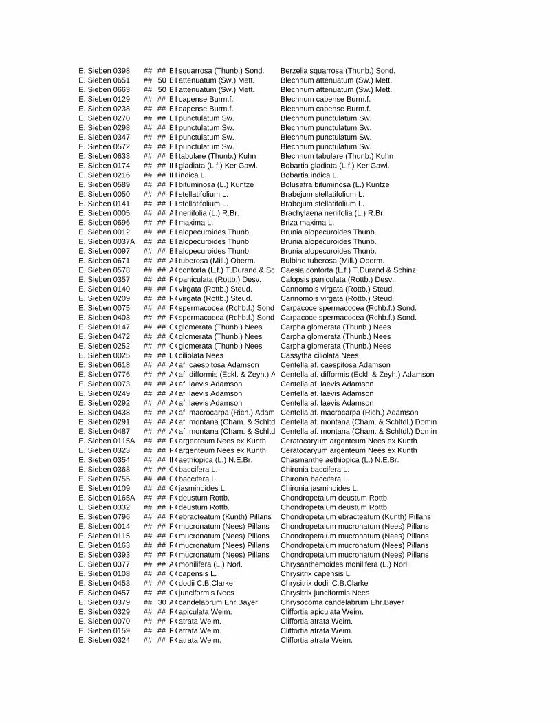
E. Sieben 0398 ## ## BBsquarrosa (Thunb.) Sond. Berzelia squarrosa (Thunb.) Sond.E. Sieben 0651 ## 50 BBattenuatum (Sw.) Mett. Blechnum attenuatum (Sw.) Mett.E. Sieben 0663 ## 50 BBattenuatum (Sw.) Mett. Blechnum attenuatum (Sw.) Mett.E. Sieben 0129 ## ## BBcapense Burm.f. Blechnum capense Burm.f.E. Sieben 0238 ## ## BBcapense Burm.f. Blechnum capense Burm.f.E. Sieben 0270 ## ## BBpunctulatum Sw. Blechnum punctulatum Sw.E. Sieben 0298 ## ## BBpunctulatum Sw. Blechnum punctulatum Sw.E. Sieben 0347 ## ## BBpunctulatum Sw. Blechnum punctulatum Sw.E. Sieben 0572 ## ## BBpunctulatum Sw. Blechnum punctulatum Sw.E. Sieben 0633 ## ## BBtabulare (Thunb.) Kuhn Blechnum tabulare (Thunb.) KuhnE. Sieben 0174 ## ## IRBgladiata (L.f.) Ker Gawl. Bobartia gladiata (L.f.) Ker Gawl.E. Sieben 0216 ## ## IRBindica L. Bobartia indica L.E. Sieben 0589 ## ## F Bbituminosa (L.) Kuntze Bolusafra bituminosa (L.) KuntzeE. Sieben 0050 ## ## PBstellatifolium L. Brabejum stellatifolium L.E. Sieben 0141 ## ## PBstellatifolium L. Brabejum stellatifolium L.E. Sieben 0005 ## ## ABneriifolia (L.) R.Br. Brachylaena neriifolia (L.) R.Br.E. Sieben 0696 ## ## PBmaxima L. Briza maxima L.E. Sieben 0012 ## ## BBalopecuroides Thunb. Brunia alopecuroides Thunb.E. Sieben 0037A ## ## BBalopecuroides Thunb. Brunia alopecuroides Thunb.E. Sieben 0097 ## ## BBalopecuroides Thunb. Brunia alopecuroides Thunb.E. Sieben 0671 ## ## ABtuberosa (Mill.) Oberm. Bulbine tuberosa (Mill.) Oberm.E. Sieben 0578 ## ## ACcontorta (L.f.) T.Durand & Sc Caesia contorta (L.f.) T.Durand & SchinzE. Sieben 0357 ## ## RCpaniculata (Rottb.) Desv. Calopsis paniculata (Rottb.) Desv.E. Sieben 0140 ## ## RCvirgata (Rottb.) Steud. Cannomois virgata (Rottb.) Steud.E. Sieben 0209 ## ## RCvirgata (Rottb.) Steud. Cannomois virgata (Rottb.) Steud.E. Sieben 0075 ## ## RCspermacocea (Rchb.f.) Sond. Carpacoce spermacocea (Rchb.f.) Sond.E. Sieben 0403 ## ## RCspermacocea (Rchb.f.) Sond. Carpacoce spermacocea (Rchb.f.) Sond.E. Sieben 0147 ## ## CCglomerata (Thunb.) Nees Carpha glomerata (Thunb.) NeesE. Sieben 0472 ## ## CCglomerata (Thunb.) Nees Carpha glomerata (Thunb.) NeesE. Sieben 0252 ## ## CCglomerata (Thunb.) Nees Carpha glomerata (Thunb.) NeesE. Sieben 0025 ## ## L Cciliolata Nees Cassytha ciliolata NeesE. Sieben 0618 ## ## ACaf. caespitosa Adamson Centella af. caespitosa AdamsonE. Sieben 0776 ## ## ACaf. difformis (Eckl. & Zeyh.) A Centella af. difformis (Eckl. & Zeyh.) AdamsonE. Sieben 0073 ## ## ACaf. laevis Adamson Centella af. laevis AdamsonE. Sieben 0249 ## ## ACaf. laevis Adamson Centella af. laevis AdamsonE. Sieben 0292 ## ## ACaf. laevis Adamson Centella af. laevis AdamsonE. Sieben 0438 ## ## ACaf. macrocarpa (Rich.) Adams Centella af. macrocarpa (Rich.) AdamsonE. Sieben 0291 ## ## ACaf. montana (Cham. & Schltd Centella af. montana (Cham. & Schltdl.) DominE. Sieben 0487 ## ## ACaf. montana (Cham. & Schltd Centella af. montana (Cham. & Schltdl.) DominE. Sieben 0115A ## ## RCargenteum Nees ex Kunth Ceratocaryum argenteum Nees ex KunthE. Sieben 0323 ## ## RCargenteum Nees ex Kunth Ceratocaryum argenteum Nees ex KunthE. Sieben 0354 ## ## IRCaethiopica (L.) N.E.Br. Chasmanthe aethiopica (L.) N.E.Br.E. Sieben 0368 ## ## GCbaccifera L. Chironia baccifera L.E. Sieben 0755 ## ## GCbaccifera L. Chironia baccifera L.E. Sieben 0109 ## ## GCjasminoides L. Chironia jasminoides L.E. Sieben 0165A ## ## RCdeustum Rottb. Chondropetalum deustum Rottb.E. Sieben 0332 ## ## RCdeustum Rottb. Chondropetalum deustum Rottb.E. Sieben 0796 ## ## RCebracteatum (Kunth) Pillans Chondropetalum ebracteatum (Kunth) PillansE. Sieben 0014 ## ## RCmucronatum (Nees) Pillans Chondropetalum mucronatum (Nees) PillansE. Sieben 0115 ## ## RCmucronatum (Nees) Pillans Chondropetalum mucronatum (Nees) PillansE. Sieben 0163 ## ## RCmucronatum (Nees) Pillans Chondropetalum mucronatum (Nees) PillansE. Sieben 0393 ## ## RCmucronatum (Nees) Pillans Chondropetalum mucronatum (Nees) PillansE. Sieben 0377 ## ## ACmonilifera (L.) Norl. Chrysanthemoides monilifera (L.) Norl.E. Sieben 0108 ## ## CCcapensis L. Chrysitrix capensis L.E. Sieben 0453 ## ## CCdodii C.B.Clarke Chrysitrix dodii C.B.ClarkeE. Sieben 0457 ## ## CCjunciformis Nees Chrysitrix junciformis NeesE. Sieben 0379 ## 30 ACcandelabrum Ehr.Bayer Chrysocoma candelabrum Ehr.BayerE. Sieben 0329 ## ## RCapiculata Weim. Cliffortia apiculata Weim.E. Sieben 0070 ## ## RCatrata Weim. Cliffortia atrata Weim.E. Sieben 0159 ## ## RCatrata Weim. Cliffortia atrata Weim.E. Sieben 0324 ## ## RCatrata Weim. Cliffortia atrata Weim.
E. Sieben 0417 ## ## RCatrata Weim. Cliffortia atrata Weim.E. Sieben 0441 ## ## RCatrata Weim. Cliffortia atrata Weim.E. Sieben 0516 ## ## RCatrata Weim. Cliffortia atrata Weim.E. Sieben 0520 ## ## RCcomplanata E.Mey. Cliffortia complanata E.Mey.E. Sieben 0718 ## ## RCcomplanata E.Mey. Cliffortia complanata E.Mey.E. Sieben 0747 ## ## RCcomplanata E.Mey. Cliffortia complanata E.Mey.E. Sieben 0244 ## ## RCcuneata Aiton Cliffortia cuneata AitonE. Sieben 0214 ## ## RCdodecandra Weim. Cliffortia dodecandra Weim.E. Sieben 0435 ## ## RCdodecandra Weim. Cliffortia dodecandra Weim.E. Sieben 0555 ## ## RCeriocephalina Cham. Cliffortia eriocephalina Cham.E. Sieben 0744 ## ## RCgraminea L.f. Cliffortia graminea L.f.E. Sieben 0213 ## ## RCgrandifolia Eckl. & Zeyh. Cliffortia grandifolia Eckl. & Zeyh.E. Sieben 0016 ## ## RChirsuta Eckl. & Zeyh. Cliffortia hirsuta Eckl. & Zeyh.E. Sieben 0808 ## ## RCintegerrima Weim. Cliffortia integerrima Weim.E. Sieben 0583 ## ## RCodorata L.f. Cliffortia odorata L.f.E. Sieben 0802 ## ## RCovalis Weim. Cliffortia ovalis Weim.E. Sieben 0625 ## ## RCovalis Weim. Cliffortia ovalis Weim.E. Sieben 0051 ## ## RCpedunculata Schltr. Cliffortia pedunculata Schltr.E. Sieben 0243 ## ## RCpolygonifolia L. Cliffortia polygonifolia L.E. Sieben 0726 ## ## RCpolygonifolia L. Cliffortia polygonifolia L.E. Sieben 0184 ## ## RCruscifolia L. Cliffortia ruscifolia L.E. Sieben 0070A ## ## RCcf. sericea Eckl. & Zeyh. Cliffortia cf. sericea Eckl. & Zeyh.E. Sieben 0697 ## ## RCstrobilifera Murray Cliffortia strobilifera MurrayE. Sieben 0643 ## ## RCtricuspidata Harv. Cliffortia tricuspidata Harv.E. Sieben 0586 ## ## ECalaternoides L. Clutia alaternoides L.E. Sieben 0596 ## ## ECalaternoides L. Clutia alaternoides L.E. Sieben 0316 ## ## EClaxa Eckl. ex Sond. Clutia laxa Eckl. ex Sond.E. Sieben 0237A ## ## ECpolygonoides L. Clutia polygonoides L.E. Sieben 0607 ## ## ECpolygonoides L. Clutia polygonoides L.E. Sieben 0794 ## ## ECpolygonoides L. Clutia polygonoides L.E. Sieben 0673 ## ## ECrubricaulis Eckl. ex Sond. Clutia rubricaulis Eckl. ex Sond.E. Sieben 0759 ## ## ECrubricaulis Eckl. ex Sond. Clutia rubricaulis Eckl. ex Sond.E. Sieben 0432 ## ## RCjuniperinum Sond. Coleonema juniperinum Sond.E. Sieben 0482 ## ## ACscabrida DC. Conyza scabrida DC.E. Sieben 0568 ## ## ACscabrida DC. Conyza scabrida DC.E. Sieben 0626 ## ## ACcongestum E.Mey. ex DC. Corymbium congestum E.Mey. ex DC.E. Sieben 0091 ## ## ACcymosum E.Mey. ex DC. Corymbium cymosum E.Mey. ex DC.E. Sieben 0266 ## ## ACcymosum E.Mey. ex DC. Corymbium cymosum E.Mey. ex DC.E. Sieben 0496 ## ## ACvillosum L.f. Corymbium villosum L.f.E. Sieben 0573 ## ACturbinata L. Cotula turbinata L.E. Sieben 0519 ## ## CCcapensis (L.) Baill. Crassula capensis (L.) Baill.E. Sieben 0521 ## ## CCcapensis (L.) Baill. Crassula capensis (L.) Baill.E. Sieben 0193 ## ## CCdejecta Jacq. Crassula dejecta Jacq.E. Sieben 0758 ## ## CCdejecta Jacq. Crassula dejecta Jacq.E. Sieben 0824 ## ## CCdejecta Jacq. Crassula dejecta Jacq.E. Sieben 0514 ## ## CCmuscosa L. Crassula muscosa L.E. Sieben 0532 ## ## CCnudicaulis L. Crassula nudicaulis L.E. Sieben 0242 ## ## ACsetosa (L.) R.Br. Cullumia setosa (L.) R.Br.E. Sieben 0801 ## ## ACsetosa (L.) R.Br. Cullumia setosa (L.) R.Br.E. Sieben 0820 ## ## ACsetosa (L.) R.Br. Cullumia setosa (L.) R.Br.E. Sieben 0142 ## ## CCcapensis L. Cunonia capensis L.E. Sieben 0811 ## ## CCdentata (Burm.f.) C.A.Sm. Curtisia dentata (Burm.f.) C.A.Sm.E. Sieben 0713 ## ## CCnitida E. Mey. ex Choisy Cuscuta nitida E. Mey. ex ChoisyE. Sieben 0653 ## ## CCcapensis (L.f.) Sm. Cyathea capensis (L.f.) Sm.E. Sieben 0655 ## ## CCcapensis (L.f.) Sm. Cyathea capensis (L.f.) Sm.E. Sieben 0672 ## ## F Cmaculata (Andrews) Kies Cyclopia maculata (Andrews) KiesE. Sieben 0675 ## ## F Cmaculata (Andrews) Kies Cyclopia maculata (Andrews) KiesE. Sieben 0502 ## ## PCcf. marginatus (Steud.) Stapf Cymbopogon cf. marginatus (Steud.) Stapf ex Burtt DavyE. Sieben 0588 ## ## CCdenudatus L.f. Cyperus denudatus L.f.E. Sieben 0818 ## ## CCfastigiatus Rottb. Cyperus fastigiatus Rottb.E. Sieben 0372 ## ## L Cvolubilis (Burm.f.) Willd. Cyphia volubilis (Burm.f.) Willd.
E. Sieben 0484 ## ## L Cvolubilis (Burm.f.) Willd. Cyphia volubilis (Burm.f.) Willd.E. Sieben 0590 ## ## L Cvolubilis (Burm.f.) Willd. Cyphia volubilis (Burm.f.) Willd.E. Sieben 0800 ## ## HDviscosa L.f. Dilatris viscosa L.f.E. Sieben 0752 ## ## RDcf. hirsuta L. Diosma cf. hirsuta L.E. Sieben 0806 ## ## RDthyrsophora Eckl. & Zeyh. Diosma thyrsophora Eckl. & Zeyh.E. Sieben 0263 ## ## EDglabra (L.) De Winter Diospyros glabra (L.) De WinterE. Sieben 0296 ## ## EDglabra (L.) De Winter Diospyros glabra (L.) De WinterE. Sieben 0200 ## ## EDglabra (L.) De Winter Diospyros glabra (L.) De WinterE. Sieben 0813 ## ## EDwhyteana (Hiern) F.White Diospyros whyteana (Hiern) F.WhiteE. Sieben 0304 ## ## F Dlignosus (L.) Verdc. Dipogon lignosus (L.) Verdc.E. Sieben 0717 ## ## ODtripetaloides (L.f.) N.E.Br. Disa tripetaloides (L.f.) N.E.Br.E. Sieben 0535 ## ## F Ddecumbens Thunb. Dolichos decumbens Thunb.E. Sieben 0040 ## ## DDaliciae Raym.-Hamet Drosera aliciae Raym.-HametE. Sieben 0707 ## ## DDcapensis L. Drosera capensis L.E. Sieben 0719 ## ## DDglabripes (Harv.) Stein Drosera glabripes (Harv.) SteinE. Sieben 0334 ## ## AEpinifolia (Lam.) Hilliard Edmondia pinifolia (Lam.) HilliardE. Sieben 0624 ## ## AEpinifolia (Lam.) Hilliard Edmondia pinifolia (Lam.) HilliardE. Sieben 0132 ## ## PEerecta Lam. Ehrharta erecta Lam.E. Sieben 0388 ## ## PEerecta Lam. Ehrharta erecta Lam.E. Sieben 0597 ## ## PEerecta Lam. Ehrharta erecta Lam.E. Sieben 0074 ## ## PErehmannii Stapf Ehrharta rehmannii StapfE. Sieben 0597 ## ## PErehmannii Stapf Ehrharta rehmannii StapfE. Sieben 0454 ## ## PEsetacea Nees subsp. setacea Ehrharta setacea Nees subsp. setaceaE. Sieben 0465 ## ## PEsetacea Nees subsp. uniflora Ehrharta setacea Nees subsp. uniflora (Burch. ex Stapf) GE. Sieben 0547 ## ## PEsetacea Nees subsp. uniflora Ehrharta setacea Nees subsp. uniflora (Burch. ex Stapf) GE. Sieben 0551 ## ## PEsetacea Nees subsp. uniflora Ehrharta setacea Nees subsp. uniflora (Burch. ex Stapf) GE. Sieben 0541 ## ## L Eangustatum (Schrad.) Hieron Elaphoglossum angustatum (Schrad.) Hieron.E. Sieben 0342 ## ## L Econforme (Sw.) J.Sm. Elaphoglossum conforme (Sw.) J.Sm.E. Sieben 0236 ## ## REasperiflora (Nees) Kunth Elegia asperiflora (Nees) KunthE. Sieben 0127 ## ## REcapensis (Burm.f.) Schelpe Elegia capensis (Burm.f.) SchelpeE. Sieben 0830 ## ## REgrandis (Nees) Kunth Elegia grandis (Nees) KunthE. Sieben 0021 ## ## REintermedia (Steud.) Pillans Elegia intermedia (Steud.) PillansE. Sieben 0543 ## ## REintermedia (Steud.) Pillans Elegia intermedia (Steud.) PillansE. Sieben 0550 ## ## REintermedia (Steud.) Pillans Elegia intermedia (Steud.) PillansE. Sieben 0645 ## ## REintermedia (Steud.) Pillans Elegia intermedia (Steud.) PillansE. Sieben 0060 ## ## REneesii Mast. Elegia neesii Mast.E. Sieben 0156 ## ## REpersistens Mast. Elegia persistens Mast.E. Sieben 0630 ## ## REracemosa (Poir.) Pers. Elegia racemosa (Poir.) Pers.E. Sieben 0638 ## ## REracemosa (Poir.) Pers. Elegia racemosa (Poir.) Pers.E. Sieben 0642 ## ## REracemosa (Poir.) Pers. Elegia racemosa (Poir.) Pers.E. Sieben 0178 ## ## REspathacea Mast. Elegia spathacea Mast.E. Sieben 0402 ## ## REspathacea Mast. Elegia spathacea Mast.E. Sieben 0706 ## ## REspathacea Mast. Elegia spathacea Mast.E. Sieben 0792 ## ## REspathacea Mast. Elegia spathacea Mast.E. Sieben 0049 ## ## AElongifolius (DC.) Levyns Elytropappus longifolius (DC.) LevynsE. Sieben 0264 ## ## REunicapsulare (L.f.) Skeels Empleurum unicapsulare (L.f.) SkeelsE. Sieben 0632 ## ## CEcomplanatus Levyns Epischoenus complanatus LevynsE. Sieben 0775 ## ## CEquadrangularis (Boeck.) C.B. Epischoenus quadrangularis (Boeck.) C.B.ClarkeE. Sieben 0451 ## ## CEvillosus Levyns Epischoenus villosus LevynsE. Sieben 0866 ## ## CEvillosus Levyns Epischoenus villosus LevynsE. Sieben 0868 ## ## CEvillosus Levyns Epischoenus villosus LevynsE. Sieben 0300 ## ## PEcurvula (Schrad.) Nees Eragrostis curvula (Schrad.) NeesE. Sieben 0613 ## ## EEautumnalis L.Bolus Erica autumnalis L.BolusE. Sieben 0631 ## ## EEautumnalis L.Bolus Erica autumnalis L.BolusE. Sieben 0647 ## ## EEautumnalis L.Bolus Erica autumnalis L.BolusE. Sieben 0470 ## ## EEcaffra L. Erica caffra L.E. Sieben 0602 ## ## EEcalycina L. Erica calycina L.E. Sieben 0600 ## ## EEcoccinea L. Erica coccinea L.E. Sieben 0859 ## ## EEcorifolia L. Erica corifolia L.E. Sieben 0741 ## ## EEcurviflora L. Erica curviflora L.E. Sieben 0080 ## ## EEcurvirostris Salisb. Erica curvirostris Salisb.
E. Sieben 0106 ## ## EEcurvirostris Salisb. Erica curvirostris Salisb.E. Sieben 0187 ## ## EEcurvirostris Salisb. Erica curvirostris Salisb.E. Sieben 0601 ## ## EEfastigiata L. Erica fastigiata L.E. Sieben 0059 ## ## EEhispidula L. Erica hispidula L.E. Sieben 0082 ## ## EEhispidula L. Erica hispidula L.E. Sieben 0407 ## ## EEhispidula L. Erica hispidula L.E. Sieben 0545 ## ## EEhispidula L. Erica hispidula L.E. Sieben 0437 ## ## EEimbricata L. Erica imbricata L.E. Sieben 0409 ## ## EEintervallaris Salisb. Erica intervallaris Salisb.E. Sieben 0449 ## ## EEintervallaris Salisb. Erica intervallaris Salisb.E. Sieben 0621 ## ## EEintervallaris Salisb. Erica intervallaris Salisb.E. Sieben 0418 ## ## EElongifolia Aiton Erica longifolia AitonE. Sieben 0473 ## ## EElucida Salisb. Erica lucida Salisb.E. Sieben 0117 ## ## EElutea P.J.Bergius Erica lutea P.J.BergiusE. Sieben 0223 ## ## EEnudiflora L. Erica nudiflora L.E. Sieben 0048 ## ## EEequisetifolia Erica equisetifoliaE. Sieben 0081 ## ## EEequisetifolia Erica equisetifoliaE. Sieben 0399 ## ## EEequisetifolia Erica equisetifoliaE. Sieben 0777 ## ## EEequisetifolia Erica equisetifoliaE. Sieben 0842 ## ## EEpinea Thunb. Erica pinea Thunb.E. Sieben 0621A ## ## EEplukenetii L. Erica plukenetii L.E. Sieben 0107 ## ## EEsessiliflora L.f. Erica sessiliflora L.f.E. Sieben 0603 ## ## EEsitiens Klotzsch Erica sitiens KlotzschE. Sieben 0773 ## ## EEsitiens Klotzsch Erica sitiens KlotzschE. Sieben 0295 ## ## EEsphaeroidea Dulfer Erica sphaeroidea DulferE. Sieben 0750 ## ## EEstrigosa Sol. Erica strigosa Sol.E. Sieben 0181 ## ## EEtegulifolia Salisb. Erica tegulifolia Salisb.E. Sieben 0259 ## ## EEtriflora L. Erica triflora L.E. Sieben 0646 ## ## EEtriflora L. Erica triflora L.E. Sieben 0829 ## ## REglabra I.Williams Euchaetis glabra I.WilliamsE. Sieben 0314 ## ## EEepicyparissias E.Mey. ex Bois Euphorbia epicyparissias E.Mey. ex Boiss.E. Sieben 0504 ## ## AEabrotanifolius Euryops abrotanifoliusE. Sieben 0415 ## ## AErupestris Schltr. Euryops rupestris Schltr.E. Sieben 0505 ## ## AErupestris Schltr. Euryops rupestris Schltr.E. Sieben 0557 ## ## AFcymbalariae (Aiton) Bolus & WFelicia cymbalariae (Aiton) Bolus & Wolley-Dod ex AdamsE. Sieben 0714 ## ## AFcf. hyssopifolia (P.J.Bergius) Felicia cf. hyssopifolia (P.J.Bergius) NeesE. Sieben 0310 ## ## CFacuminata (Nees) Nees Ficinia acuminata (Nees) NeesE. Sieben 0467 ## ## CFacuminata (Nees) Nees Ficinia acuminata (Nees) NeesE. Sieben 0528 ## ## CFacuminata (Nees) Nees Ficinia acuminata (Nees) NeesE. Sieben 0677 ## ## CFacuminata (Nees) Nees Ficinia acuminata (Nees) NeesE. Sieben 0867 ## ## CFargyropa Nees Ficinia argyropa NeesE. Sieben 0869 ## ## CFargyropa Nees Ficinia argyropa NeesE. Sieben 0700 ## ## CFbrevifolia Nees ex Kunth Ficinia brevifolia Nees ex KunthE. Sieben 0756 ## ## CFbrevifolia Nees ex Kunth Ficinia brevifolia Nees ex KunthE. Sieben 0561 ## ## CFdistans C.B.Clarke Ficinia distans C.B.ClarkeE. Sieben 0577 ## ## CFdistans C.B.Clarke Ficinia distans C.B.ClarkeE. Sieben 0669 ## ## CFdistans C.B.Clarke Ficinia distans C.B.ClarkeE. Sieben 0439 ## ## CFfiliformis (Lam.) Schrad. Ficinia filiformis (Lam.) Schrad.E. Sieben 0424 ## ## CFnigrescens (Schrad.) J.Rayna Ficinia nigrescens (Schrad.) J.RaynalE. Sieben 0478 ## ## CFnigrescens (Schrad.) J.Rayna Ficinia nigrescens (Schrad.) J.RaynalE. Sieben 0507 ## ## CFnigrescens (Schrad.) J.Rayna Ficinia nigrescens (Schrad.) J.RaynalE. Sieben 0312 ## ## CFoligantha (Steud.) J.Raynal Ficinia oligantha (Steud.) J.RaynalE. Sieben 0459 ## ## CFramosissima Kunth Ficinia ramosissima KunthE. Sieben 0137 ## ## CFtrichodes (Schrad.) Benth. & Ficinia trichodes (Schrad.) Benth. & Hook.f.E. Sieben 0235 ## ## CFtrichodes (Schrad.) Benth. & Ficinia trichodes (Schrad.) Benth. & Hook.f.E. Sieben 0490 ## ## CFtrichodes (Schrad.) Benth. & Ficinia trichodes (Schrad.) Benth. & Hook.f.E. Sieben 0581 ## ## F Fmuralis Sond. ex W.D.J.Koch Fumaria muralis Sond. ex W.D.J.KochE. Sieben 0822 ## ## AGsubfalcata (Cabrera) Cabrera Gamochaeta subfalcata (Cabrera) CabreraE. Sieben 0522 ## ## IRGovalifolia R.C.Foster Geissorhiza ovalifolia R.C.FosterE. Sieben 0617 ## ## IRGumbrosa G.J.Lewis Geissorhiza umbrosa G.J.LewisE. Sieben 0202 ## ## AGilicifolia (L.) Norl. Gibbaria ilicifolia (L.) Norl.
E. Sieben 0442 ## ## AGilicifolia (L.) Norl. Gibbaria ilicifolia (L.) Norl.E. Sieben 0667 ## ## IRGcarneus D.Delaroche Gladiolus carneus D.DelarocheE. Sieben 0787 ## ## IRGcarneus D.Delaroche Gladiolus carneus D.DelarocheE. Sieben 0795 ## ## IRGcarneus D.Delaroche Gladiolus carneus D.DelarocheE. Sieben 0222 ## ## GGpolypodioides (L.) Sm. Gleichenia polypodioides (L.) Sm.E. Sieben 0376 ## ## AGprolifera (Burm.f.) B.L.Burtt Glia prolifera (Burm.f.) B.L.BurttE. Sieben 0839 ## ## AGprolifera (Burm.f.) B.L.Burtt Glia prolifera (Burm.f.) B.L.BurttE. Sieben 0229 ## ## T Gcf. anomala Meisn. Gnidia cf. anomala Meisn.E. Sieben 0608 ## ## T Ggalpinii C.H.Wright Gnidia galpinii C.H.WrightE. Sieben 0774 ## ## T Ggalpinii C.H.Wright Gnidia galpinii C.H.WrightE. Sieben 0803 ## ## T Ggalpinii C.H.Wright Gnidia galpinii C.H.WrightE. Sieben 0413 ## ## T Goppositifolia L. Gnidia oppositifolia L.E. Sieben 0039 ## ## GGrosmarinifolia P.J.Bergius Grubbia rosmarinifolia P.J.BergiusE. Sieben 0448 ## ## GGrosmarinifolia P.J.Bergius Grubbia rosmarinifolia P.J.BergiusE. Sieben 0709 ## ## GGrosmarinifolia P.J.Bergius Grubbia rosmarinifolia P.J.BergiusE. Sieben 0847 ## ## PHsericea Schrad. Hakea sericea Schrad.E. Sieben 0282 ## ## SHelliptica Thunb. Halleria elliptica Thunb.E. Sieben 0546 ## ## SHlucida L. Halleria lucida L.E. Sieben 0294 ## ## AHlanata (Thunb.) Less. Haplocarpha lanata (Thunb.) Less.E. Sieben 0189 ## ## CHschinoides (Spreng.) Codd Hartogiella schinoides (Spreng.) CoddE. Sieben 0255 ## ## CHschinoides (Spreng.) Codd Hartogiella schinoides (Spreng.) CoddE. Sieben 0764 ## ## AHargentea (Thunb.) Meisn. Heeria argentea (Thunb.) Meisn.E. Sieben 0192 ## ## AHcymosum (L.) D.Don Helichrysum cymosum (L.) D.DonE. Sieben 0297 ## ## AHcymosum (L.) D.Don Helichrysum cymosum (L.) D.DonE. Sieben 0692 ## ## AHcymosum (L.) D.Don Helichrysum cymosum (L.) D.DonE. Sieben 0118 ## ## AHfelinum Less. Helichrysum felinum Less.E. Sieben 0770 ## ## AHfoetidum (L.) Moench Helichrysum foetidum (L.) MoenchE. Sieben 0821 ## ## AHfoetidum (L.) Moench Helichrysum foetidum (L.) MoenchE. Sieben 0565 ## ## AHhelianthemifolium (L.) D.Don Helichrysum helianthemifolium (L.) D.DonE. Sieben 0594 ## ## AHhelianthemifolium (L.) D.Don Helichrysum helianthemifolium (L.) D.DonE. Sieben 0690 ## ## AHhelianthemifolium (L.) D.Don Helichrysum helianthemifolium (L.) D.DonE. Sieben 0360 ## ## AHpatulum (L.) D.Don Helichrysum patulum (L.) D.DonE. Sieben 0525 ## ## AHtinctum (Thunb.) Hilliard & B. Helichrysum tinctum (Thunb.) Hilliard & B.L.BurttE. Sieben 0584 ## ## SHmontana L.f. Hemimeris montana L.f.E. Sieben 0585 ## ## SHalnifolia L. Hermannia alnifolia L.E. Sieben 0426 ## ## AHaliena (L.f.) Druce Heterolepis aliena (L.f.) DruceE. Sieben 0595 ## ## MHtrionum L. Hibiscus trionum L.E. Sieben 0553 ## ## AHbolusae Hutch. Hippia bolusae Hutch.E. Sieben 0331 ## ## AHcf. frutescens (L.) L. Hippia cf. frutescens (L.) L.E. Sieben 0676 ## ## AHcf. frutescens (L.) L. Hippia cf. frutescens (L.) L.E. Sieben 0566 ## ## DHincisa (Thunb.) J.Sm. Histiopteris incisa (Thunb.) J.Sm.E. Sieben 0427 ## ## OHvillosa Lindl. Holothrix villosa Lindl.E. Sieben 0538 ## ## OHvillosa Lindl. Holothrix villosa Lindl.E. Sieben 0476 ## ## IRHcollina (Thunb.) Salisb. Homeria collina (Thunb.) Salisb.E. Sieben 0529 ## ## IRHcollina (Thunb.) Salisb. Homeria collina (Thunb.) Salisb.E. Sieben 0650 ## ## HHmarlothii Brause Hymenophyllum marlothii BrauseE. Sieben 0275 ## ## HHpeltatum (Poir.) Desv. Hymenophyllum peltatum (Poir.) Desv.E. Sieben 0560 ## ## F Hsophoroides (P.J.Bergius) Ba Hypocalyptus sophoroides (P.J.Bergius) Baill.E. Sieben 0211 ## ## AHradicata L. Hypochoeris radicata L.E. Sieben 0840 ## ## AHradicata L. Hypochoeris radicata L.E. Sieben 0889 ## ## AHradicata L. Hypochoeris radicata L.E. Sieben 0620 ## ## RHaristatus (Thunb.) Krauss Hypodiscus aristatus (Thunb.) KraussE. Sieben 0563 ## ## DHsparsisora (Schrad.) Kuhn Hypolepis sparsisora (Schrad.) KuhnE. Sieben 0124 ## ## AI mitis (L.) Radlk. Ilex mitis (L.) Radlk.E. Sieben 0276 ## ## AI mitis (L.) Radlk. Ilex mitis (L.) Radlk.E. Sieben 0158 ## ## RI cincinnata (Mast.) H.P.Linder Ischyrolepis cincinnata (Mast.) H.P.LinderE. Sieben 0863 ## ## RI curviramis (Kunth) H.P.Linde Ischyrolepis curviramis (Kunth) H.P.LinderE. Sieben 0359 ## ## RI gaudichaudiana (Kunth) H.P. Ischyrolepis gaudichaudiana (Kunth) H.P.LinderE. Sieben 0486 ## ## RI gaudichaudiana (Kunth) H.P. Ischyrolepis gaudichaudiana (Kunth) H.P.LinderE. Sieben 0877 ## ## RI gaudichaudiana (Kunth) H.P. Ischyrolepis gaudichaudiana (Kunth) H.P.LinderE. Sieben 0023 ## ## RI gaudichaudiana (Kunth) H.P. Ischyrolepis gaudichaudiana (Kunth) H.P.Linder
E. Sieben 0793 ## ## RI helenae (Mast.) H.P.Linder Ischyrolepis helenae (Mast.) H.P.LinderE. Sieben 0041 ## ## RI subverticillata Steud. Ischyrolepis subverticillata Steud.E. Sieben 0861 ## ## RI subverticillata Steud. Ischyrolepis subverticillata Steud.E. Sieben 0069 ## ## RI triflora (Rottb.) H.P.Linder Ischyrolepis triflora (Rottb.) H.P.LinderE. Sieben 0791 ## ## RI triflora (Rottb.) H.P.Linder Ischyrolepis triflora (Rottb.) H.P.LinderE. Sieben 0711 ## ## CI digitata Schrad. Isolepis digitata Schrad.E. Sieben 0691 ## ## CI fluitans (L.) R.Br. Isolepis fluitans (L.) R.Br.E. Sieben 0854 ## ## CI fluitans (L.) R.Br. Isolepis fluitans (L.) R.Br.E. Sieben 0679 ## ## CI prolifer R.Br. Isolepis prolifer R.Br.E. Sieben 0681 ## ## J Jcapensis Thunb. Juncus capensis Thunb.E. Sieben 0684 ## ## J Jcephalotes Thunb. Juncus cephalotes Thunb.E. Sieben 0701 ## ## J Jeffusus L. Juncus effusus L.E. Sieben 0245 ## ## J Jlomatophyllus Spreng. Juncus lomatophyllus Spreng.E. Sieben 0340 ## ## J Jlomatophyllus Spreng. Juncus lomatophyllus Spreng.E. Sieben 0277 ## ## F Kafricana L. Kiggelaria africana L.E. Sieben 0382 ## ## F Kafricana L. Kiggelaria africana L.E. Sieben 0389 ## ## F Kafricana L. Kiggelaria africana L.E. Sieben 0564 ## ## F Kafricana L. Kiggelaria africana L.E. Sieben 0552 ## ## AKtabularis Marloth Kniphofia tabularis MarlothE. Sieben 0825 ## ## RKcapensis (L.) Huth Knowltonia capensis (L.) HuthE. Sieben 0509 ## ## RKvesicatoria (L.f.) Sims Knowltonia vesicatoria (L.f.) SimsE. Sieben 0595A ## ## ALserriola L. Lactuca serriola L.E. Sieben 0727 ## ## HLrepens P.J.Bergius subsp. br Laurembergia repens P.J.Bergius subsp. brachypoda (HieE. Sieben 0682 ## ## L Larabidea (C.Presl) A.DC. Laurentia arabidea (C.Presl) A.DC.E. Sieben 0591 ## ## L Lleonurus (L.) R.Br. Leonotis leonurus (L.) R.Br.E. Sieben 0412 ## ## PLcf. gandogeri Schinz ex Gand Leucadendron cf. gandogeri Schinz ex Gand.E. Sieben 0046 ## ## PLcf. laureolum (Lam.) Fourc. Leucadendron cf. laureolum (Lam.) Fourc.E. Sieben 0886 ## ## PLcf. laureolum (Lam.) Fourc. Leucadendron cf. laureolum (Lam.) Fourc.E. Sieben 0809 ## ## PLmicrocephalum (Gand.) Gand Leucadendron microcephalum (Gand.) Gand. & SchinzE. Sieben 0122 ## ## PLxanthoconus (Kuntze) K.Schu Leucadendron xanthoconus (Kuntze) K.Schum.E. Sieben 0493 ## ## ALlacera Cham. & Schltdl. Lichtensteinia lacera Cham. & Schltdl.E. Sieben 0283 ## ## CLparvifolia (P.J.Bergius) Adam Lightfootia parvifolia (P.J.Bergius) AdamsonE. Sieben 0580 ## ## L Lerinus L. Lobelia erinus L.E. Sieben 0639 ## ## L Ljasionoides (A.DC.) E.Wimm. Lobelia jasionoides (A.DC.) E.Wimm.E. Sieben 0054 20 ## L Lcarolinianum L. Lycopodium carolinianum L.E. Sieben 0888 20 ## L Lclavatum L. Lycopodium clavatum L.E. Sieben 0852 ## ## RMdigitata (Thunb.) Gilg-Ben. Mastersiella digitata (Thunb.) Gilg-Ben.E. Sieben 0387 ## ## CMacuminata (L.f.) Loes. Maytenus acuminata (L.f.) Loes.E. Sieben 0390 ## ## CMoleoides (Lam.) Loes. Maytenus oleoides (Lam.) Loes.E. Sieben 0679 ## ## PMcincta (Nees) Conert Merxmuellera cincta (Nees) ConertE. Sieben 0083 ## ## AMcephalotes (Thunb.) Less. Metalasia cephalotes (Thunb.) Less.E. Sieben 0172 ## ## AMcephalotes (Thunb.) Less. Metalasia cephalotes (Thunb.) Less.E. Sieben 0406 ## ## AMcephalotes (Thunb.) Less. Metalasia cephalotes (Thunb.) Less.E. Sieben 0527 ## ## AMcephalotes (Thunb.) Less. Metalasia cephalotes (Thunb.) Less.E. Sieben 0446 ## ## AMdensa (Lam.) P.O.Karis Metalasia densa (Lam.) P.O.KarisE. Sieben 0125 ## ## MMangustifolia (L.) Sm. Metrosideros angustifolia (L.) Sm.E. Sieben 0301 ## ## SMcaffrorum (L.) Desv. Mohria caffrorum (L.) Desv.E. Sieben 0683 ## ## L Mlutea (L.) Urb. Monopsis lutea (L.) Urb.E. Sieben 0494 ## ## MMcaryophyllacea Thunb. Montinia caryophyllacea Thunb.E. Sieben 0367 ## ## PMalba Levyns Muraltia alba LevynsE. Sieben 0230 ## ## PMheisteria (L.) DC. Muraltia heisteria (L.) DC.E. Sieben 0205 ## ## PMheisteria (L.) DC. Muraltia heisteria (L.) DC.E. Sieben 0498 ## ## PMvulpina Chodat Muraltia vulpina ChodatE. Sieben 0686 ## ## MMserrata Lam. Myrica serrata Lam.E. Sieben 0303 ## ## MMafricana L. Myrsine africana L.E. Sieben 0512 ## ## MMafricana L. Myrsine africana L.E. Sieben 0518 ## ## AMscandens (Thunb.) Oberm. Myrsiphyllum scandens (Thunb.) Oberm.E. Sieben 0570 ## ## AMvolubile (Thunb.) Oberm. Myrsiphyllum volubile (Thunb.) Oberm.E. Sieben 0571 ## ## AMvolubile (Thunb.) Oberm. Myrsiphyllum volubile (Thunb.) Oberm.E. Sieben 0401 ## ## BNfragarioides (Willd.) Kuntze Nebelia fragarioides (Willd.) KuntzeE. Sieben 0045 ## ## CNpunctoria (Vahl) Levyns Neesenbeckia punctoria (Vahl) Levyns
E. Sieben 0042 ## ## RNobtusissima (Steud.) H.P.Lind Nevillea obtusissima (Steud.) H.P.LinderE. Sieben 0474 ## ## SOafricana (L.) Bocq. Oftia africana (L.) Bocq.E. Sieben 0544 ## ## OOcapensis L. Olea capensis L.E. Sieben 0812 ## ## OOcapensis L. Olea capensis L.E. Sieben 0662 ## ## OOeuropaea L. subsp. africana ( Olea europaea L. subsp. africana (Mill.) P.S.GreenE. Sieben 0814 ## ## OOventosa (L.) Cufod. Olinia ventosa (L.) Cufod.E. Sieben 0443 ## ## AOafra (L.) K.Bremer Osmitopsis afra (L.) K.BremerE. Sieben 0834 ## ## AOpinnatifida (DC.) K.Bremer Osmitopsis pinnatifida (DC.) K.BremerE. Sieben 0315 ## ## AOciliatum P.J.Bergius Osteospermum ciliatum P.J.BergiusE. Sieben 0582 ## ## AOciliatum P.J.Bergius Osteospermum ciliatum P.J.BergiusE. Sieben 0492 ## ## F Oobliquum (E.Mey.) C.H.Stirt. Otholobium obliquum (E.Mey.) C.H.Stirt.E. Sieben 0674 ## ## F Oobliquum (E.Mey.) C.H.Stirt. Otholobium obliquum (E.Mey.) C.H.Stirt.E. Sieben 0526 ## ## AOparviflora P.J.Bergius Othonna parviflora P.J.BergiusE. Sieben 0113 ## ## AOquinquedentata Thunb. Othonna quinquedentata Thunb.E. Sieben 0197 ## ## AOquinquedentata Thunb. Othonna quinquedentata Thunb.E. Sieben 0531 ## ## OOcf. corniculata L. Oxalis cf. corniculata L.E. Sieben 0272 ## ## OOcf. dentata Jacq. Oxalis cf. dentata Jacq.E. Sieben 0365 ## ## OOlanata L.f. Oxalis lanata L.f.E. Sieben 0364 ## ## OOlivida Jacq. Oxalis livida Jacq.E. Sieben 0219 ## ## OOcf. nidulans Eckl. & Zeyh. Oxalis cf. nidulans Eckl. & Zeyh.E. Sieben 0317 ## ## OOcf. nidulans Eckl. & Zeyh. Oxalis cf. nidulans Eckl. & Zeyh.E. Sieben 0363 ## ## OOpurpurea L. Oxalis purpurea L.E. Sieben 0513 ## ## OOpurpurea L. Oxalis purpurea L.E. Sieben 0444 ## ## OOtruncatula Jacq. Oxalis truncatula Jacq.E. Sieben 0485 ## ## OOtruncatula Jacq. Oxalis truncatula Jacq.E. Sieben 0495 ## ## OOcf. versicolor L. Oxalis cf. versicolor L.E. Sieben 0723 ## ## PPmaximum Jacq. Panicum maximum Jacq.E. Sieben 0730 ## ## PPurvillei Steud. Paspalum urvillei Steud.E. Sieben 0823 ## ## PPurvillei Steud. Paspalum urvillei Steud.E. Sieben 0728 ## ## T Pvulgaris Thoday Passerina vulgaris ThodayE. Sieben 0587 ## ## GPcolumbinum Jacq. Pelargonium columbinum Jacq.E. Sieben 0284 ## ## GPcucullatum (L.) L'Hér. Pelargonium cucullatum (L.) L'Hér.E. Sieben 0576 ## ## GPelongatum (Cav.) Salisb. Pelargonium elongatum (Cav.) Salisb.E. Sieben 0250 ## ## GPhermanniifolium (P.J.Bergius Pelargonium hermanniifolium (P.J.Bergius) Jacq.E. Sieben 0306 ## ## GPpatulum Jacq. Pelargonium patulum Jacq.E. Sieben 0506 ## ## GPpatulum Jacq. Pelargonium patulum Jacq.E. Sieben 0844 ## ## GPpatulum Jacq. Pelargonium patulum Jacq.E. Sieben 0349 ## ## GPtomentosum Jacq. Pelargonium tomentosum Jacq.E. Sieben 0188 ## ## APpteroides (L.) Prantl Pellaea pteroides (L.) PrantlE. Sieben 0712 ## ## PPcneorum Meerb. Penaea cneorum Meerb.E. Sieben 0221 ## ## PPmucronata L. Penaea mucronata L.E. Sieben 0687 ## ## PPmacrourum Trin. Pennisetum macrourum Trin.E. Sieben 0734 ## 50 PPdistichophylla (Lehm.) Nees Pentameris distichophylla (Lehm.) NeesE. Sieben 0628 ## ## PPhirtiglumis N.P.Barker Pentameris hirtiglumis N.P.BarkerE. Sieben 0629 ## ## PPhirtiglumis N.P.Barker Pentameris hirtiglumis N.P.BarkerE. Sieben 0416 ## ## PPmacrocalycina (Steud.) Schw Pentameris macrocalycina (Steud.) Schweick.E. Sieben 0857 ## ## PPobtusifolia (Hochst.) Schweic Pentameris obtusifolia (Hochst.) Schweick.E. Sieben 0206 ## ## PPthuarii P.Beauv. Pentameris thuarii P.Beauv.E. Sieben 0464 ## ## PPthuarii P.Beauv. Pentameris thuarii P.Beauv.E. Sieben 0479 ## ## PPthuarii P.Beauv. Pentameris thuarii P.Beauv.E. Sieben 0240 ## ## PPampla (Nees) McClean Pentaschistis ampla (Nees) McCleanE. Sieben 0761 ## ## PPampla (Nees) McClean Pentaschistis ampla (Nees) McCleanE. Sieben 0112 ## ## PPcurvifolia (Schrad.) Stapf Pentaschistis curvifolia (Schrad.) StapfE. Sieben 0688 ## ## PPdensifolia (Nees) Stapf Pentaschistis densifolia (Nees) StapfE. Sieben 0430 ## ## PPholciformis (Nees) H.P.Linder Pentaschistis holciformis (Nees) H.P.LinderE. Sieben 0853 ## ## PPholciformis (Nees) H.P.Linder Pentaschistis holciformis (Nees) H.P.LinderE. Sieben 0088 ## ## PPmalouinensis (Steud.) Clayto Pentaschistis malouinensis (Steud.) ClaytonE. Sieben 0720 ## ## PPmalouinensis (Steud.) Clayto Pentaschistis malouinensis (Steud.) ClaytonE. Sieben 0885 ## ## PPmalouinensis (Steud.) Clayto Pentaschistis malouinensis (Steud.) ClaytonE. Sieben 0333 ## ## PPpallida (Thunb.) H.P.Linder Pentaschistis pallida (Thunb.) H.P.LinderE. Sieben 0337 ## ## PPpallida (Thunb.) H.P.Linder Pentaschistis pallida (Thunb.) H.P.Linder
E. Sieben 0530 ## ## PPpallida (Thunb.) H.P.Linder Pentaschistis pallida (Thunb.) H.P.LinderE. Sieben 0668 ## ## PPpallida (Thunb.) H.P.Linder Pentaschistis pallida (Thunb.) H.P.LinderE. Sieben 0716 ## ## PPpallida (Thunb.) H.P.Linder Pentaschistis pallida (Thunb.) H.P.LinderE. Sieben 0703 ## ## APgalbaniopse H.Wolff Peucedanum galbaniopse H.WolffE. Sieben 0182 ## ## APgalbanum (L.) Drude Peucedanum galbanum (L.) DrudeE. Sieben 0475 ## ## APcf. strictum (Spreng.) B.L.Bur Peucedanum cf. strictum (Spreng.) B.L.BurttE. Sieben 0419 ## ## APprolifera (L.) D.Don Phaenocoma prolifera (L.) D.DonE. Sieben 0836 ## ## RPcallosa L.f. Phylica callosa L.f.E. Sieben 0425 ## ## RPericoides L. Phylica ericoides L.E. Sieben 0860 ## ## RPericoides L. Phylica ericoides L.E. Sieben 0237 ## ## RPgracilis (Eckl. & Zeyh.) D.Diet Phylica gracilis (Eckl. & Zeyh.) D.Dietr.E. Sieben 0760 ## ## RPimberbis P.J.Bergius Phylica imberbis P.J.BergiusE. Sieben 0862 ## ## RPimberbis P.J.Bergius Phylica imberbis P.J.BergiusE. Sieben 0705 ## ## RPplumosa L. Phylica plumosa L.E. Sieben 0738 ## ## PPcf. pinaster Aiton Pinus cf. pinaster AitonE. Sieben 0386 ## ## PPundulatum Vent. Pittosporum undulatum Vent.E. Sieben 0135 ## ## RPcallistachyus (Kunth) H.P.Lind Platycaulos callistachyus (Kunth) H.P.LinderE. Sieben 0859 ## ## RPcallistachyus (Kunth) H.P.Lind Platycaulos callistachyus (Kunth) H.P.LinderE. Sieben 0785 ## ## RPcascadensis (Pillans) H.P.Lin Platycaulos cascadensis (Pillans) H.P.LinderE. Sieben 0644 ## ## RPdepauperatus (Kunth) H.P.Lin Platycaulos depauperatus (Kunth) H.P.LinderE. Sieben 0742 ## ## RPdepauperatus (Kunth) H.P.Lin Platycaulos depauperatus (Kunth) H.P.LinderE. Sieben 0148 ## ## CPtrifoliatus (L.f.) D.Don Platylophus trifoliatus (L.f.) D.DonE. Sieben 0261 ## ## APpolifolia (Thunb.) Hilliard & B. Plecostachys polifolia (Thunb.) Hilliard & B.L.BurttE. Sieben 0099 ## ## F Pcalyptrata (Retz.) Willd. Podalyria calyptrata (Retz.) Willd.E. Sieben 0616 ## ## F Pmontana Hutch. Podalyria montana Hutch.E. Sieben 0816 ## ## PPcf. elongatus (Aiton) L'H‚r. ex Podocarpus cf. elongatus (Aiton) L'H‚r. ex Pers.E. Sieben 0666 ## ## PPlatifolius (Thunb.) R.Br. ex Mi Podocarpus latifolius (Thunb.) R.Br. ex Mirb.E. Sieben 0816A ## ## PPlatifolius (Thunb.) R.Br. ex Mi Podocarpus latifolius (Thunb.) R.Br. ex Mirb.E. Sieben 0085 ## ## PPcf. nematocaulis Levyns Polygala cf. nematocaulis LevynsE. Sieben 0845 ## ## F Pcapitata DC. Priestleya capitata DC.E. Sieben 0152 ## ## J Pserratum (L.f.) DrŠge ex E.Me Prionium serratum (L.f.) DrŠge ex E.Mey.E. Sieben 0875 ## ## J Pserratum (L.f.) DrŠge ex E.Me Prionium serratum (L.f.) DrŠge ex E.Mey.E. Sieben 0469 ## ## APretrofractus (L.) Oberm. Protasparagus retrofractus (L.) Oberm.E. Sieben 0486 ## ## APrubicundus (P.J.Bergius) Obe Protasparagus rubicundus (P.J.Bergius) Oberm.E. Sieben 0884 ## ## PPamplexicaulis (Salisb.) R.Br. Protea amplexicaulis (Salisb.) R.Br.E. Sieben 0065 ## ## PPcynaroides (L.) L. Protea cynaroides (L.) L.E. Sieben 0810 ## ## PPgrandiceps Tratt. Protea grandiceps Tratt.E. Sieben 0423 ## ## PPlongifolia Andrews Protea longifolia AndrewsE. Sieben 0422 ## ## PPmundii Klotzsch Protea mundii KlotzschE. Sieben 0704 ## ## PPneriifolia R.Br. Protea neriifolia R.Br.E. Sieben 0767 ## ## PPnitida Mill. Protea nitida Mill.E. Sieben 0004 ## ## BPafricana (Burm.f.) Pillans Pseudobaeckea africana (Burm.f.) PillansE. Sieben 0408 ## ## BPafricana (Burm.f.) Pillans Pseudobaeckea africana (Burm.f.) PillansE. Sieben 0094 ## F Paculeata Psoralea aculeataE. Sieben 0440 ## ## F Paphylla L. Psoralea aphylla L.E. Sieben 0574 ## ## F Pasarina (P.J.Bergius) Salter Psoralea asarina (P.J.Bergius) SalterE. Sieben 0134 ## F Paf. fleta C. H. Stirton Psoralea af. fleta C. H. StirtonE. Sieben 0471 ## F Paf. fleta C. H. Stirton Psoralea af. fleta C. H. StirtonE. Sieben 0575 ## ## F Ppinnata L. Psoralea pinnata L.E. Sieben 0126 ## ## DPaquilinum (L.) Kuhn Pteridium aquilinum (L.) KuhnE. Sieben 0569 ## ## CProstratus Walp. Pterocelastrus rostratus Walp.E. Sieben 0540 ## ## MRmelanophloeos (L.) Mez Rapanea melanophloeos (L.) MezE. Sieben 0783 ## ## BRmicrophylla (Thunb.) Brongn. Raspalia microphylla (Thunb.) Brongn.E. Sieben 0649 ## ## BRvirgata (Brongn.) Pillans Raspalia virgata (Brongn.) PillansE. Sieben 0320 ## ## RRbifarius Mast. Restio bifarius Mast.E. Sieben 0874 ## ## RRbifidus Thunb. Restio bifidus Thunb.E. Sieben 0827 ## ## RRbifurcus Nees ex Mast. Restio bifurcus Nees ex Mast.E. Sieben 0790 ## ## RRburchellii Pillans Restio burchellii PillansE. Sieben 0848 ## ## RRburchellii Pillans Restio burchellii PillansE. Sieben 0400 ## ## RRcorneolus Esterh. Restio corneolus Esterh.E. Sieben 0322 ## ## RRcorneolus Esterh. Restio corneolus Esterh.
E. Sieben 0420 ## ## RRdebilis Nees Restio debilis NeesE. Sieben 0326 ## ## RRdegenerans Pillans Restio degenerans PillansE. Sieben 0463 ## ## RRdegenerans Pillans Restio degenerans PillansE. Sieben 0548 ## ## RRdegenerans Pillans Restio degenerans PillansE. Sieben 0780 ## ## RRdegenerans Pillans Restio degenerans PillansE. Sieben 0843 ## ## RRdispar Mast. Restio dispar Mast.E. Sieben 0165 ## ## RRechinatus Kunth Restio echinatus KunthE. Sieben 0850 ## ## RRegregius Hochst. Restio egregius Hochst.E. Sieben 0851 ## ## RRegregius Hochst. Restio egregius Hochst.E. Sieben 0604 ## ## RRejuncidus Mast. Restio ejuncidus Mast.E. Sieben 0533 ## ## RRfiliformis Poir. Restio filiformis Poir.E. Sieben 0431 ## ## RRnuwebergensis Esterh. Restio nuwebergensis Esterh.E. Sieben 0154 ## ## RRoccultus (Mast.) Pillans Restio occultus (Mast.) PillansE. Sieben 0066 ## ## RRcf. perplexus Kunth Restio cf. perplexus KunthE. Sieben 0724 ## ## RRcf. perplexus Kunth Restio cf. perplexus KunthE. Sieben 0881 ## ## RRcf. perplexus Kunth Restio cf. perplexus KunthE. Sieben 0022 ## ## RRpurpurascens Nees ex Mast. Restio purpurascens Nees ex Mast.E. Sieben 0247 ## ## RRquadratus Mast. Restio quadratus Mast.E. Sieben 0799 ## ## RRstokoei Pillans Restio stokoei PillansE. Sieben 0450 ## ## RRsubtilis Nees ex Mast. Restio subtilis Nees ex Mast.E. Sieben 0456 ## ## RRaf. versatilis H.P.Linder Restio af. versatilis H.P.LinderE. Sieben 0605 ## ## RRaf. versatilis H.P.Linder Restio af. versatilis H.P.LinderE. Sieben 0615 ## ## RRaf. versatilis H.P.Linder Restio af. versatilis H.P.LinderE. Sieben 0251 ## ## ARangustifolia L. Rhus angustifolia L.E. Sieben 0351 ## ## ARtomentosa L. Rhus tomentosa L.E. Sieben 0779 ## ## CRdregeana A.DC. Roella dregeana A.DC.E. Sieben 0361 ## ## RRcf. pinnatus Willd. Rubus cf. pinnatus Willd.E. Sieben 0680 ## ## RRcf. rigidus Sm. Rubus cf. rigidus Sm.E. Sieben 0350 ## ## L Schamelaeagnea P.J.Bergius Salvia chamelaeagnea P.J.BergiusE. Sieben 0104 ## ## SSpectinata (L.) Sw. Schizaea pectinata (L.) Sw.E. Sieben 0029 ## ## SStenella Kaulf. Schizaea tenella Kaulf.E. Sieben 0253 ## ## CSlanceum (Thunb.) Kük. Schoenoxiphium lanceum (Thunb.) Kük.E. Sieben 0273 ## ## CSlanceum (Thunb.) Kük. Schoenoxiphium lanceum (Thunb.) Kük.E. Sieben 0285 ## ## CSlanceum (Thunb.) Kük. Schoenoxiphium lanceum (Thunb.) Kük.E. Sieben 0383 ## ## CSlanceum (Thunb.) Kük. Schoenoxiphium lanceum (Thunb.) Kük.E. Sieben 0508 ## ## CSlanceum (Thunb.) Kük. Schoenoxiphium lanceum (Thunb.) Kük.E. Sieben 0749 ## ## ESmicrantha (Benth.) N.E.Br. Scyphogyne micrantha (Benth.) N.E.Br.E. Sieben 0879 ## ## ESmicrantha (Benth.) N.E.Br. Scyphogyne micrantha (Benth.) N.E.Br.E. Sieben 0754 ## ## ASalpini Schult. Secamone alpini Schult.E. Sieben 0290 ## ## SSserrata P.J.Bergius Selago serrata P.J.BergiusE. Sieben 0370 ## ## SSserrata P.J.Bergius Selago serrata P.J.BergiusE. Sieben 0817 ## ## SSserrata P.J.Bergius Selago serrata P.J.BergiusE. Sieben 0768 ## ## ASamabilis DC. Senecio amabilis DC.E. Sieben 0461 ## ## AScoleophyllus Turcz. Senecio coleophyllus Turcz.E. Sieben 0558 ## ## AScrispus Thunb. Senecio crispus Thunb.E. Sieben 0743 ## ## AScrispus Thunb. Senecio crispus Thunb.E. Sieben 0556 ## ## ASgrandiflorus P.J.Bergius Senecio grandiflorus P.J.BergiusE. Sieben 0356 ## ## AScf. hastatus L. Senecio cf. hastatus L.E. Sieben 0689 ## ## AScf. hastatus L. Senecio cf. hastatus L.E. Sieben 0517 ## ## ASpinnulatus Thunb. Senecio pinnulatus Thunb.E. Sieben 0693 ## ## ASpinnulatus Thunb. Senecio pinnulatus Thunb.E. Sieben 0819 ## ## ASpterophorus DC. Senecio pterophorus DC.E. Sieben 0870 ## ## ASpubigerus L. Senecio pubigerus L.E. Sieben 0634 ## ## ASsubcanescens (DC.) Compto Senecio subcanescens (DC.) ComptonE. Sieben 0694 ## ## AScf. vulgaris L. Senecio cf. vulgaris L.E. Sieben 0567 ## ## SSretroflexum Dunal Solanum retroflexum DunalE. Sieben 0397 ## ## RScernua (L.f.) T.Durand & Sch Staberoha cernua (L.f.) T.Durand & SchinzE. Sieben 0610 ## ## RScf. vaginata (Thunb.) Pillans Staberoha cf. vaginata (Thunb.) PillansE. Sieben 0614 ## ## RScf. vaginata (Thunb.) Pillans Staberoha cf. vaginata (Thunb.) PillansE. Sieben 0593 ## ## L Saethiopica L. Stachys aethiopica L.E. Sieben 0339 ## ## SSmucronata N.E.Br. Stilbe mucronata N.E.Br.
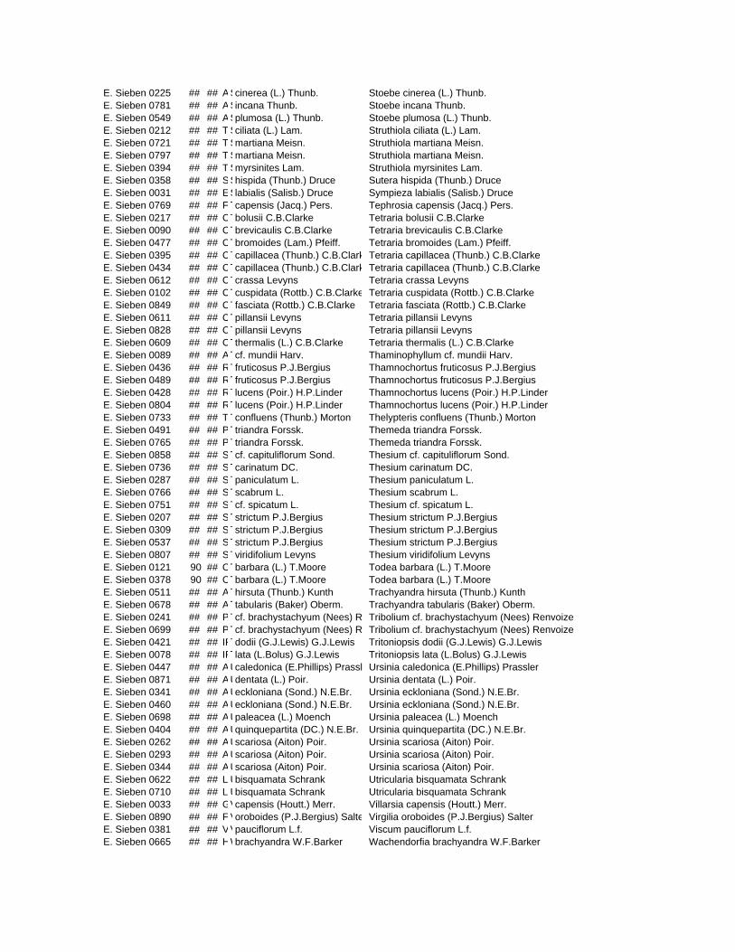
E. Sieben 0225 ## ## AScinerea (L.) Thunb. Stoebe cinerea (L.) Thunb.E. Sieben 0781 ## ## ASincana Thunb. Stoebe incana Thunb.E. Sieben 0549 ## ## ASplumosa (L.) Thunb. Stoebe plumosa (L.) Thunb.E. Sieben 0212 ## ## T Sciliata (L.) Lam. Struthiola ciliata (L.) Lam.E. Sieben 0721 ## ## T Smartiana Meisn. Struthiola martiana Meisn.E. Sieben 0797 ## ## T Smartiana Meisn. Struthiola martiana Meisn.E. Sieben 0394 ## ## T Smyrsinites Lam. Struthiola myrsinites Lam.E. Sieben 0358 ## ## SShispida (Thunb.) Druce Sutera hispida (Thunb.) DruceE. Sieben 0031 ## ## ESlabialis (Salisb.) Druce Sympieza labialis (Salisb.) DruceE. Sieben 0769 ## ## F Tcapensis (Jacq.) Pers. Tephrosia capensis (Jacq.) Pers.E. Sieben 0217 ## ## CTbolusii C.B.Clarke Tetraria bolusii C.B.ClarkeE. Sieben 0090 ## ## CTbrevicaulis C.B.Clarke Tetraria brevicaulis C.B.ClarkeE. Sieben 0477 ## ## CTbromoides (Lam.) Pfeiff. Tetraria bromoides (Lam.) Pfeiff.E. Sieben 0395 ## ## CTcapillacea (Thunb.) C.B.Clark Tetraria capillacea (Thunb.) C.B.ClarkeE. Sieben 0434 ## ## CTcapillacea (Thunb.) C.B.Clark Tetraria capillacea (Thunb.) C.B.ClarkeE. Sieben 0612 ## ## CTcrassa Levyns Tetraria crassa LevynsE. Sieben 0102 ## ## CTcuspidata (Rottb.) C.B.Clarke Tetraria cuspidata (Rottb.) C.B.ClarkeE. Sieben 0849 ## ## CTfasciata (Rottb.) C.B.Clarke Tetraria fasciata (Rottb.) C.B.ClarkeE. Sieben 0611 ## ## CTpillansii Levyns Tetraria pillansii LevynsE. Sieben 0828 ## ## CTpillansii Levyns Tetraria pillansii LevynsE. Sieben 0609 ## ## CTthermalis (L.) C.B.Clarke Tetraria thermalis (L.) C.B.ClarkeE. Sieben 0089 ## ## ATcf. mundii Harv. Thaminophyllum cf. mundii Harv.E. Sieben 0436 ## ## RTfruticosus P.J.Bergius Thamnochortus fruticosus P.J.BergiusE. Sieben 0489 ## ## RTfruticosus P.J.Bergius Thamnochortus fruticosus P.J.BergiusE. Sieben 0428 ## ## RTlucens (Poir.) H.P.Linder Thamnochortus lucens (Poir.) H.P.LinderE. Sieben 0804 ## ## RTlucens (Poir.) H.P.Linder Thamnochortus lucens (Poir.) H.P.LinderE. Sieben 0733 ## ## T Tconfluens (Thunb.) Morton Thelypteris confluens (Thunb.) MortonE. Sieben 0491 ## ## PTtriandra Forssk. Themeda triandra Forssk.E. Sieben 0765 ## ## PTtriandra Forssk. Themeda triandra Forssk.E. Sieben 0858 ## ## STcf. capituliflorum Sond. Thesium cf. capituliflorum Sond.E. Sieben 0736 ## ## STcarinatum DC. Thesium carinatum DC.E. Sieben 0287 ## ## STpaniculatum L. Thesium paniculatum L.E. Sieben 0766 ## ## STscabrum L. Thesium scabrum L.E. Sieben 0751 ## ## STcf. spicatum L. Thesium cf. spicatum L.E. Sieben 0207 ## ## STstrictum P.J.Bergius Thesium strictum P.J.BergiusE. Sieben 0309 ## ## STstrictum P.J.Bergius Thesium strictum P.J.BergiusE. Sieben 0537 ## ## STstrictum P.J.Bergius Thesium strictum P.J.BergiusE. Sieben 0807 ## ## STviridifolium Levyns Thesium viridifolium LevynsE. Sieben 0121 90 ## OTbarbara (L.) T.Moore Todea barbara (L.) T.MooreE. Sieben 0378 90 ## OTbarbara (L.) T.Moore Todea barbara (L.) T.MooreE. Sieben 0511 ## ## AThirsuta (Thunb.) Kunth Trachyandra hirsuta (Thunb.) KunthE. Sieben 0678 ## ## ATtabularis (Baker) Oberm. Trachyandra tabularis (Baker) Oberm.E. Sieben 0241 ## ## PTcf. brachystachyum (Nees) R Tribolium cf. brachystachyum (Nees) RenvoizeE. Sieben 0699 ## ## PTcf. brachystachyum (Nees) R Tribolium cf. brachystachyum (Nees) RenvoizeE. Sieben 0421 ## ## IRTdodii (G.J.Lewis) G.J.Lewis Tritoniopsis dodii (G.J.Lewis) G.J.LewisE. Sieben 0078 ## ## IRTlata (L.Bolus) G.J.Lewis Tritoniopsis lata (L.Bolus) G.J.LewisE. Sieben 0447 ## ## AUcaledonica (E.Phillips) Prassl Ursinia caledonica (E.Phillips) PrasslerE. Sieben 0871 ## ## AUdentata (L.) Poir. Ursinia dentata (L.) Poir.E. Sieben 0341 ## ## AUeckloniana (Sond.) N.E.Br. Ursinia eckloniana (Sond.) N.E.Br.E. Sieben 0460 ## ## AUeckloniana (Sond.) N.E.Br. Ursinia eckloniana (Sond.) N.E.Br.E. Sieben 0698 ## ## AUpaleacea (L.) Moench Ursinia paleacea (L.) MoenchE. Sieben 0404 ## ## AUquinquepartita (DC.) N.E.Br. Ursinia quinquepartita (DC.) N.E.Br.E. Sieben 0262 ## ## AUscariosa (Aiton) Poir. Ursinia scariosa (Aiton) Poir.E. Sieben 0293 ## ## AUscariosa (Aiton) Poir. Ursinia scariosa (Aiton) Poir.E. Sieben 0344 ## ## AUscariosa (Aiton) Poir. Ursinia scariosa (Aiton) Poir.E. Sieben 0622 ## ## L Ubisquamata Schrank Utricularia bisquamata SchrankE. Sieben 0710 ## ## L Ubisquamata Schrank Utricularia bisquamata SchrankE. Sieben 0033 ## ## GVcapensis (Houtt.) Merr. Villarsia capensis (Houtt.) Merr.E. Sieben 0890 ## ## F Voroboides (P.J.Bergius) Salte Virgilia oroboides (P.J.Bergius) SalterE. Sieben 0381 ## ## VVpauciflorum L.f. Viscum pauciflorum L.f.E. Sieben 0665 ## ## HWbrachyandra W.F.Barker Wachendorfia brachyandra W.F.Barker

E. Sieben 0725 ## ## HWthyrsiflora Burm. Wachendorfia thyrsiflora Burm.E. Sieben 0798 ## ## CWprocumbens (Thunb.) A.DC. Wahlenbergia procumbens (Thunb.) A.DC.E. Sieben 0831 ## ## CWprocumbens (Thunb.) A.DC. Wahlenbergia procumbens (Thunb.) A.DC.E. Sieben 0664 ## ## IRWborbonica (Pourr.) Goldblatt Watsonia borbonica (Pourr.) GoldblattE. Sieben 0855 ## ## IRWschlechteri L.Bolus Watsonia schlechteri L.BolusE. Sieben 0077 ## ## CWnodiflora (L.) Powrie Widdringtonia nodiflora (L.) PowrieE. Sieben 0789 ## ## RWsulcata Mast. Willdenowia sulcata Mast.E. Sieben 0499 ## ## AZaethiopica (L.) Spreng. Zantedeschia aethiopica (L.) Spreng.
Appendix D The transects 1 to 123 were collected in the Hottentots Holland Mountains. Each of them contains between 1 and 7 vegetation samples. The last transects, numbers 125 to 133, each with a single vegetation sample (numbers 259 to 267), were collected in several areas. Transects 125 to 128 were collected in the upper reaches of the Wit River catchment in the Dutoitskloof Mountains. Transects 129 and 130 were collected in the Groenland Mountains, nowadays also part of the Hottentots Holland Nature Reserve. Transects 131 and 132 were collected in Bains Kloof in the upper reaches of the Breede River. Transect 133 was collected on the Akkedisberg near Stanford.
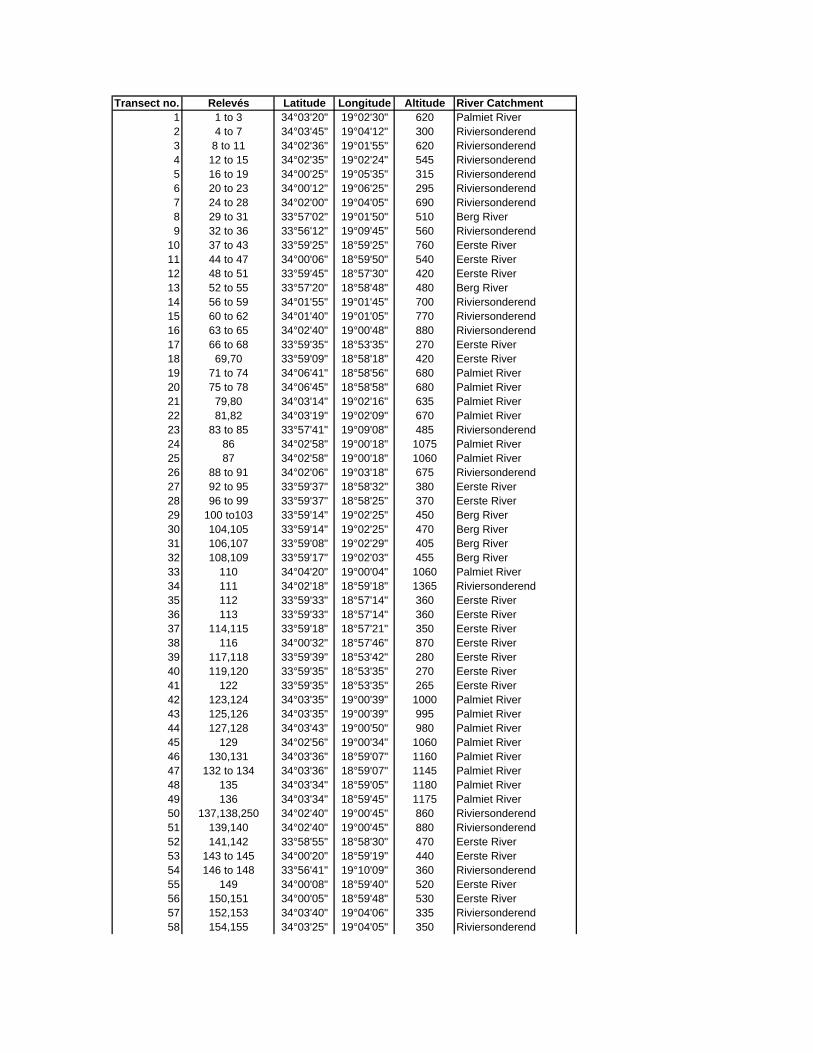
Transect no. Relevés Latitude Longitude Altitude River Catchment1 1 to 3 34°03'20" 19°02'30" 620 Palmiet River2 4 to 7 34°03'45" 19°04'12" 300 Riviersonderend3 8 to 11 34°02'36" 19°01'55" 620 Riviersonderend4 12 to 15 34°02'35" 19°02'24" 545 Riviersonderend5 16 to 19 34°00'25" 19°05'35" 315 Riviersonderend6 20 to 23 34°00'12" 19°06'25" 295 Riviersonderend7 24 to 28 34°02'00" 19°04'05" 690 Riviersonderend8 29 to 31 33°57'02" 19°01'50" 510 Berg River9 32 to 36 33°56'12" 19°09'45" 560 Riviersonderend
10 37 to 43 33°59'25" 18°59'25" 760 Eerste River11 44 to 47 34°00'06" 18°59'50" 540 Eerste River12 48 to 51 33°59'45" 18°57'30" 420 Eerste River13 52 to 55 33°57'20" 18°58'48" 480 Berg River14 56 to 59 34°01'55" 19°01'45" 700 Riviersonderend15 60 to 62 34°01'40" 19°01'05" 770 Riviersonderend16 63 to 65 34°02'40" 19°00'48" 880 Riviersonderend17 66 to 68 33°59'35" 18°53'35" 270 Eerste River18 69,70 33°59'09" 18°58'18" 420 Eerste River19 71 to 74 34°06'41" 18°58'56" 680 Palmiet River20 75 to 78 34°06'45" 18°58'58" 680 Palmiet River21 79,80 34°03'14" 19°02'16" 635 Palmiet River22 81,82 34°03'19" 19°02'09" 670 Palmiet River23 83 to 85 33°57'41" 19°09'08" 485 Riviersonderend24 86 34°02'58" 19°00'18" 1075 Palmiet River25 87 34°02'58" 19°00'18" 1060 Palmiet River26 88 to 91 34°02'06" 19°03'18" 675 Riviersonderend27 92 to 95 33°59'37" 18°58'32" 380 Eerste River28 96 to 99 33°59'37" 18°58'25" 370 Eerste River29 100 to103 33°59'14" 19°02'25" 450 Berg River30 104,105 33°59'14" 19°02'25" 470 Berg River31 106,107 33°59'08" 19°02'29" 405 Berg River32 108,109 33°59'17" 19°02'03" 455 Berg River33 110 34°04'20" 19°00'04" 1060 Palmiet River34 111 34°02'18" 18°59'18" 1365 Riviersonderend35 112 33°59'33" 18°57'14" 360 Eerste River36 113 33°59'33" 18°57'14" 360 Eerste River37 114,115 33°59'18" 18°57'21" 350 Eerste River38 116 34°00'32" 18°57'46" 870 Eerste River39 117,118 33°59'39" 18°53'42" 280 Eerste River40 119,120 33°59'35" 18°53'35" 270 Eerste River41 122 33°59'35" 18°53'35" 265 Eerste River42 123,124 34°03'35" 19°00'39" 1000 Palmiet River43 125,126 34°03'35" 19°00'39" 995 Palmiet River44 127,128 34°03'43" 19°00'50" 980 Palmiet River45 129 34°02'56" 19°00'34" 1060 Palmiet River46 130,131 34°03'36" 18°59'07" 1160 Palmiet River47 132 to 134 34°03'36" 18°59'07" 1145 Palmiet River48 135 34°03'34" 18°59'05" 1180 Palmiet River49 136 34°03'34" 18°59'45" 1175 Palmiet River50 137,138,250 34°02'40" 19°00'45" 860 Riviersonderend51 139,140 34°02'40" 19°00'45" 880 Riviersonderend52 141,142 33°58'55" 18°58'30" 470 Eerste River53 143 to 145 34°00'20" 18°59'19" 440 Eerste River54 146 to 148 33°56'41" 19°10'09" 360 Riviersonderend55 149 34°00'08" 18°59'40" 520 Eerste River56 150,151 34°00'05" 18°59'48" 530 Eerste River57 152,153 34°03'40" 19°04'06" 335 Riviersonderend58 154,155 34°03'25" 19°04'05" 350 Riviersonderend
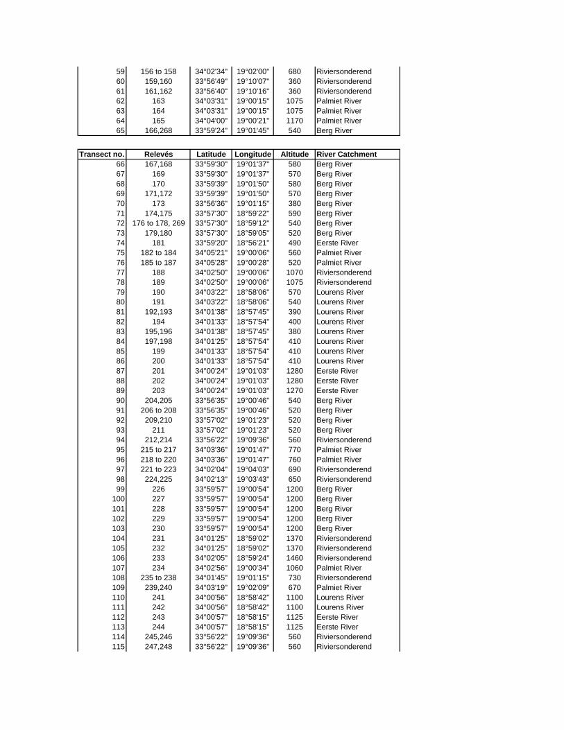
59 156 to 158 34°02'34" 19°02'00" 680 Riviersonderend60 159,160 33°56'49" 19°10'07" 360 Riviersonderend61 161,162 33°56'40" 19°10'16" 360 Riviersonderend62 163 34°03'31" 19°00'15" 1075 Palmiet River63 164 34°03'31" 19°00'15" 1075 Palmiet River64 165 34°04'00" 19°00'21" 1170 Palmiet River65 166,268 33°59'24" 19°01'45" 540 Berg River
Transect no. Relevés Latitude Longitude Altitude River Catchment66 167,168 33°59'30" 19°01'37" 580 Berg River67 169 33°59'30" 19°01'37" 570 Berg River68 170 33°59'39" 19°01'50" 580 Berg River69 171,172 33°59'39" 19°01'50" 570 Berg River70 173 33°56'36" 19°01'15" 380 Berg River71 174,175 33°57'30" 18°59'22" 590 Berg River72 176 to 178, 269 33°57'30" 18°59'12" 540 Berg River73 179,180 33°57'30" 18°59'05" 520 Berg River74 181 33°59'20" 18°56'21" 490 Eerste River75 182 to 184 34°05'21" 19°00'06" 560 Palmiet River76 185 to 187 34°05'28" 19°00'28" 520 Palmiet River77 188 34°02'50" 19°00'06" 1070 Riviersonderend78 189 34°02'50" 19°00'06" 1075 Riviersonderend79 190 34°03'22" 18°58'06" 570 Lourens River80 191 34°03'22" 18°58'06" 540 Lourens River81 192,193 34°01'38" 18°57'45" 390 Lourens River82 194 34°01'33" 18°57'54" 400 Lourens River83 195,196 34°01'38" 18°57'45" 380 Lourens River84 197,198 34°01'25" 18°57'54" 410 Lourens River85 199 34°01'33" 18°57'54" 410 Lourens River86 200 34°01'33" 18°57'54" 410 Lourens River87 201 34°00'24" 19°01'03" 1280 Eerste River88 202 34°00'24" 19°01'03" 1280 Eerste River89 203 34°00'24" 19°01'03" 1270 Eerste River90 204,205 33°56'35" 19°00'46" 540 Berg River91 206 to 208 33°56'35" 19°00'46" 520 Berg River92 209,210 33°57'02" 19°01'23" 520 Berg River93 211 33°57'02" 19°01'23" 520 Berg River94 212,214 33°56'22" 19°09'36" 560 Riviersonderend95 215 to 217 34°03'36" 19°01'47" 770 Palmiet River96 218 to 220 34°03'36" 19°01'47" 760 Palmiet River97 221 to 223 34°02'04" 19°04'03" 690 Riviersonderend98 224,225 34°02'13" 19°03'43" 650 Riviersonderend99 226 33°59'57" 19°00'54" 1200 Berg River
100 227 33°59'57" 19°00'54" 1200 Berg River101 228 33°59'57" 19°00'54" 1200 Berg River102 229 33°59'57" 19°00'54" 1200 Berg River103 230 33°59'57" 19°00'54" 1200 Berg River104 231 34°01'25" 18°59'02" 1370 Riviersonderend105 232 34°01'25" 18°59'02" 1370 Riviersonderend106 233 34°02'05" 18°59'24" 1460 Riviersonderend107 234 34°02'56" 19°00'34" 1060 Palmiet River108 235 to 238 34°01'45" 19°01'15" 730 Riviersonderend109 239,240 34°03'19" 19°02'09" 670 Palmiet River110 241 34°00'56" 18°58'42" 1100 Lourens River111 242 34°00'56" 18°58'42" 1100 Lourens River112 243 34°00'57" 18°58'15" 1125 Eerste River113 244 34°00'57" 18°58'15" 1125 Eerste River114 245,246 33°56'22" 19°09'36" 560 Riviersonderend115 247,248 33°56'22" 19°09'36" 560 Riviersonderend
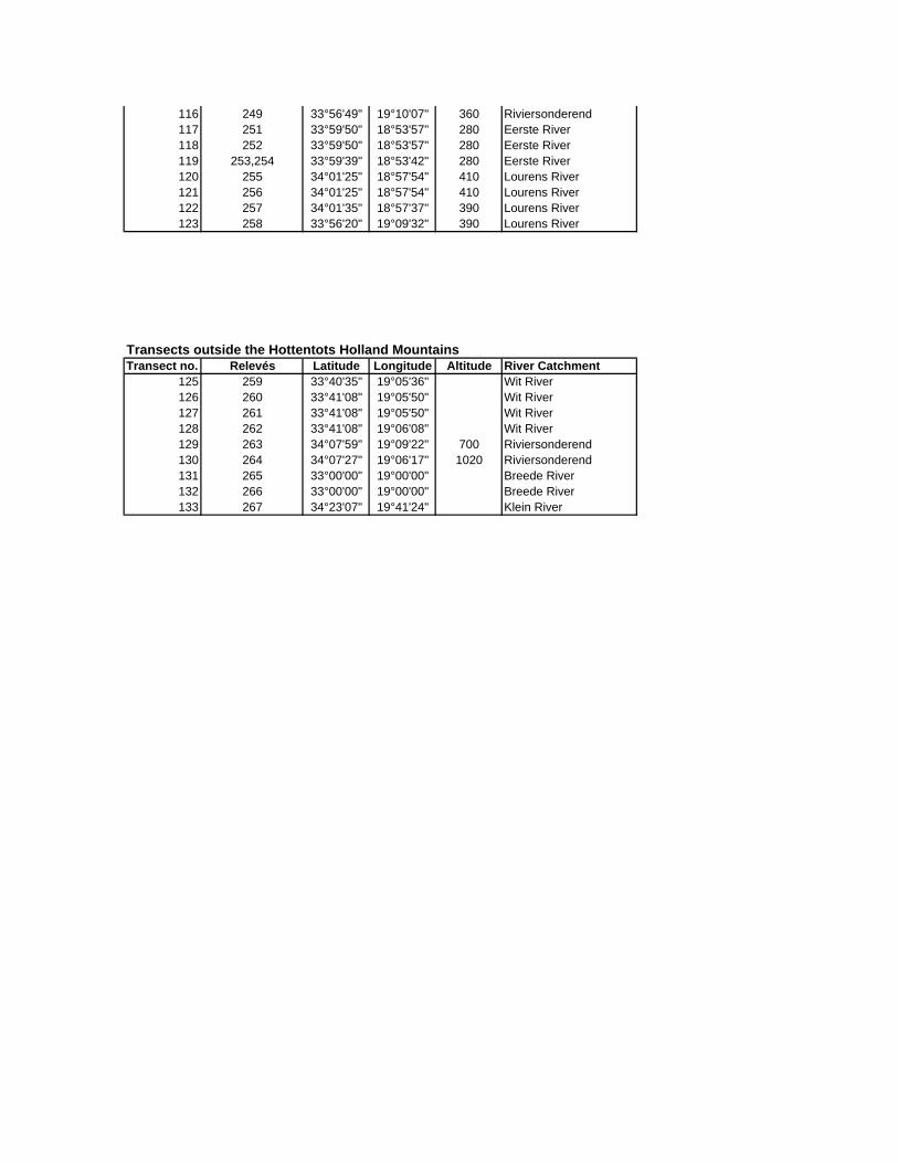
116 249 33°56'49" 19°10'07" 360 Riviersonderend117 251 33°59'50" 18°53'57" 280 Eerste River118 252 33°59'50" 18°53'57" 280 Eerste River119 253,254 33°59'39" 18°53'42" 280 Eerste River120 255 34°01'25" 18°57'54" 410 Lourens River121 256 34°01'25" 18°57'54" 410 Lourens River122 257 34°01'35" 18°57'37" 390 Lourens River123 258 33°56'20" 19°09'32" 390 Lourens River
Transects outside the Hottentots Holland MountainsTransect no. Relevés Latitude Longitude Altitude River Catchment
125 259 33°40'35" 19°05'36" Wit River126 260 33°41'08" 19°05'50" Wit River127 261 33°41'08" 19°05'50" Wit River128 262 33°41'08" 19°06'08" Wit River129 263 34°07'59" 19°09'22" 700 Riviersonderend130 264 34°07'27" 19°06'17" 1020 Riviersonderend131 265 33°00'00" 19°00'00" Breede River132 266 33°00'00" 19°00'00" Breede River133 267 34°23'07" 19°41'24" Klein River

Appendix E: Vegetation Tables Table 1: Seepage communities
Table 2: Aquatic communities
Table 3: Wet Bank communities
Table 4: Ericaceous Fynbos communities
Table 5: Asteraceous Fynbos communities
Table 6: Forest and Scrub communities
Table 7: Synoptic table
Legend: Codes for River name L: Lourens River
B: Berg River
R: Riviersonderend River
E: Eerste River
P: Palmiet River
W: Wit River
Br: tributaries of Breede River
The plant name is followed by two codes. The first of these indicates the vegetation types for which a
species is differential.
d1.2 differential for community 1.2
d1.2-4 differential for communities 1.2 to 1.4
d1 differential for community group 1
The second code indicates the stratum in which it is found. Sometimes more than one stratum is
indicated.
t3 tree layer
s1 tall shrub layer (2 – 6 m)
s2 low shrub layer (0.5 – 2 m)
hl herb layer
ml moss layer
jl juveniles
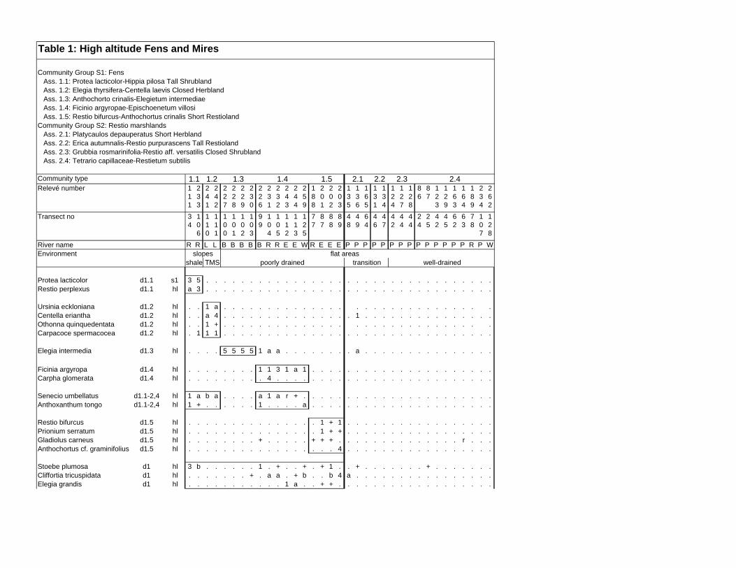
Community Group S1: Fens Ass. 1.1: Protea lacticolor-Hippia pilosa Tall Shrubland Ass. 1.2: Elegia thyrsifera-Centella laevis Closed Herbland Ass. 1.3: Anthochorto crinalis-Elegietum intermediae Ass. 1.4: Ficinio argyropae-Epischoenetum villosi Ass. 1.5: Restio bifurcus-Anthochortus crinalis Short RestiolandCommunity Group S2: Restio marshlands Ass. 2.1: Platycaulos depauperatus Short Herbland Ass. 2.2: Erica autumnalis-Restio purpurascens Tall Restioland Ass. 2.3: Grubbia rosmarinifolia-Restio aff. versatilis Closed Shrubland Ass. 2.4: Tetrario capillaceae-Restietum subtilis
Community typeRelevé number 1
11
233
241
242
227
228
229
230
226
231
232
243
244
259
188
201
202
203
135
136
165
131
134
124
127
128
86
87
123
129
163
164
189
234
262
Transect no 34
106
110
111
100
101
102
103
99
104
105
112
113
125
77
87
88
89
48
49
64
46
47
42
44
44
24
25
42
45
62
63
78
107
128
River name R R L L B B B B B R R E E W R E E E P P P P P P P P P P P P P P R P W
Protea lacticolor d1.1 s1 3 5 . . . . . . . . . . . . . . . . . . . . . . . . . . . . . . . . .Restio perplexus d1.1 hl a 3 . . . . . . . . . . . . . . . . . . . . . . . . . . . . . . . . .
Ursinia eckloniana d1.2 hl . . 1 a . . . . . . . . . . . . . . . . . . . . . . . . . . . . .Centella eriantha d1.2 hl . . a 4 . . . . . . . . . . . . . . . 1 . . . . . . . . . . . . . . .Othonna quinquedentata d1.2 hl . . 1 + . . . . . . . . . . . . . . . . . . . . . . . . . . . . .Carpacoce spermacocea d1.2 hl . 1 1 1 . . . . . . . . . . . . . . . . . . . . . . . . . . . . . . .
Elegia intermedia d1.3 hl . . . . 5 5 5 5 1 a a . . . . . . . . a . . . . . . . . . . . . . . .
Ficinia argyropa d1.4 hl . . . . . . . . 1 1 3 1 a 1 . . . . . . . . . . . . . . . . . . . . .Carpha glomerata d1.4 hl . . . . . . . . . 4 . . . . . . . . . . . . . . . . . . . . . . . . .
Senecio umbellatus d1.1-2,4 hl 1 a b a . . . . a 1 a r + . . . . . . . . . . . . . . . . . . . . . .Anthoxanthum tongo d1.1-2,4 hl 1 + . . . . . . 1 . . . . a . . . . . . . . . . . . . . . . . . . . .
Restio bifurcus d1.5 hl . . . . . . . . . . . . . . . 1 + 1 . . . . . . . . . . . . . . . . .Prionium serratum d1.5 hl . . . . . . . . . . . . . . . 1 + + . . . . . . . . . . . . . . . . .Gladiolus carneus d1.5 hl . . . . . . . . + . . . . . + + + . . . . . . . . . . . . . . r . . .Anthochortus cf. graminifolius d1.5 hl . . . . . . . . . . . . . . . . . 4 . . . . . . . . . . . . . . . . .
Stoebe plumosa d1 hl 3 b . . . . . . 1 . + . . + . + 1 . . + . . . . . . . + . . . . . . .Cliffortia tricuspidata d1 hl . . . . . . . + . a a . + b . . b 4 a . . . . . . . . . . . . . . . .Elegia grandis d1 hl . . . . . . . . . . . 1 a . . + + . . . . . . . . . . . . . . . . . .
1.2
Table 1: High altitude Fens and Mires
Environment
1.1
TMS
1.3
transition
1.4 1.5 2.1
poorly drained well-drained
2.4
slopes flat areas shale
2.2 2.3
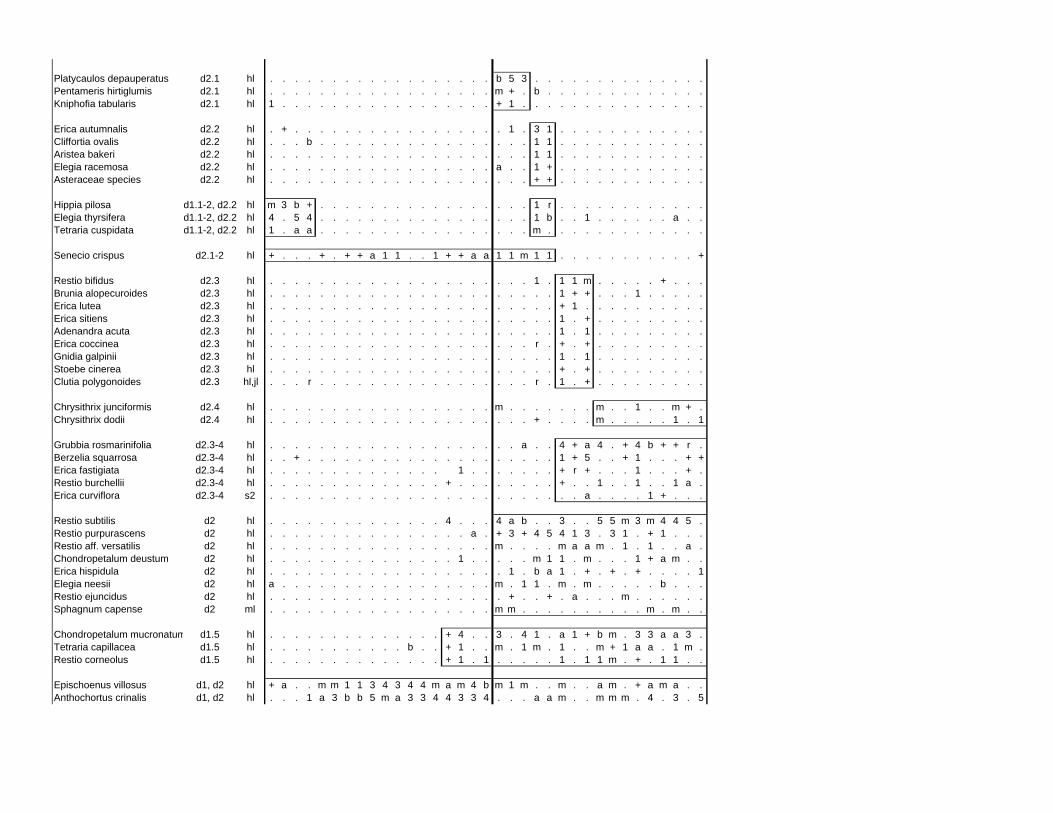
Platycaulos depauperatus d2.1 hl . . . . . . . . . . . . . . . . . . b 5 3 . . . . . . . . . . . . . .Pentameris hirtiglumis d2.1 hl . . . . . . . . . . . . . . . . . . m + . b . . . . . . . . . . . . .Kniphofia tabularis d2.1 hl 1 . . . . . . . . . . . . . . . . . + 1 . . . . . . . . . . . . . . .
Erica autumnalis d2.2 hl . + . . . . . . . . . . . . . . . . . 1 . 3 1 . . . . . . . . . . . .Cliffortia ovalis d2.2 hl . . . b . . . . . . . . . . . . . . . . . 1 1 . . . . . . . . . . . .Aristea bakeri d2.2 hl . . . . . . . . . . . . . . . . . . . . . 1 1 . . . . . . . . . . . .Elegia racemosa d2.2 hl . . . . . . . . . . . . . . . . . . a . . 1 + . . . . . . . . . . . .Asteraceae species d2.2 hl . . . . . . . . . . . . . . . . . . . . . + + . . . . . . . . . . . .
Hippia pilosa d1.1-2, d2.2 hl m 3 b + . . . . . . . . . . . . . . . . . 1 r . . . . . . . . . . . .Elegia thyrsifera d1.1-2, d2.2 hl 4 . 5 4 . . . . . . . . . . . . . . . . . 1 b . . 1 . . . . . . a . .Tetraria cuspidata d1.1-2, d2.2 hl 1 . a a . . . . . . . . . . . . . . . . . m . . . . . . . . . . . . .
Senecio crispus d2.1-2 hl + . . . + . + + a 1 1 . . 1 + + a a 1 1 m 1 1 . . . . . . . . . . . +
Restio bifidus d2.3 hl . . . . . . . . . . . . . . . . . . . . . 1 . 1 1 m . . . . . + . . .Brunia alopecuroides d2.3 hl . . . . . . . . . . . . . . . . . . . . . . . 1 + + . . . 1 . . . . .Erica lutea d2.3 hl . . . . . . . . . . . . . . . . . . . . . . . + 1 . . . . . . . . . .Erica sitiens d2.3 hl . . . . . . . . . . . . . . . . . . . . . . . 1 . + . . . . . . . . .Adenandra acuta d2.3 hl . . . . . . . . . . . . . . . . . . . . . . . 1 . 1 . . . . . . . . .Erica coccinea d2.3 hl . . . . . . . . . . . . . . . . . . . . . r . + . + . . . . . . . . .Gnidia galpinii d2.3 hl . . . . . . . . . . . . . . . . . . . . . . . 1 . 1 . . . . . . . . .Stoebe cinerea d2.3 hl . . . . . . . . . . . . . . . . . . . . . . . + . + . . . . . . . . .Clutia polygonoides d2.3 hl,jl . . . r . . . . . . . . . . . . . . . . . r . 1 . + . . . . . . . . .
Chrysithrix junciformis d2.4 hl . . . . . . . . . . . . . . . . . . m . . . . . . . m . . 1 . . m + .Chrysithrix dodii d2.4 hl . . . . . . . . . . . . . . . . . . . . . + . . . . m . . . . . 1 . 1
Grubbia rosmarinifolia d2.3-4 hl . . . . . . . . . . . . . . . . . . . . a . . 4 + a 4 . + 4 b + + r .Berzelia squarrosa d2.3-4 hl . . + . . . . . . . . . . . . . . . . . . . . 1 + 5 . . + 1 . . . + +Erica fastigiata d2.3-4 hl . . . . . . . . . . . . . . 1 . . . . . . . + r + . . . 1 . . . + .Restio burchellii d2.3-4 hl . . . . . . . . . . . . . . + . . . . . . . . + . . 1 . . 1 . . 1 a .Erica curviflora d2.3-4 s2 . . . . . . . . . . . . . . . . . . . . . . . . . a . . . . 1 + . . .
Restio subtilis d2 hl . . . . . . . . . . . . . . 4 . . . 4 a b . . 3 . . 5 5 m 3 m 4 4 5 .Restio purpurascens d2 hl . . . . . . . . . . . . . . . . a . + 3 + 4 5 4 1 3 . 3 1 . + 1 . . .Restio aff. versatilis d2 hl . . . . . . . . . . . . . . . . . . m . . . . m a a m . 1 . 1 . . a .Chondropetalum deustum d2 hl . . . . . . . . . . . . . . . 1 . . . . . m 1 1 . m . . . 1 + a m . .Erica hispidula d2 hl . . . . . . . . . . . . . . . . . . . 1 . b a 1 . + . + . + . . . . 1Elegia neesii d2 hl a . . . . . . . . . . . . . . . . . m . 1 1 . m . m . . . . . b . . .Restio ejuncidus d2 hl . . . . . . . . . . . . . . . . . . . + . . + . a . . . m . . . . . .Sphagnum capense d2 ml . . . . . . . . . . . . . . . . . . m m . . . . . . . . . . m . m . .
Chondropetalum mucronatum d1.5 hl . . . . . . . . . . . . . . + 4 . . 3 . 4 1 . a 1 + b m . 3 3 a a 3 .Tetraria capillacea d1.5 hl . . . . . . . . . . . b . . + 1 . . m . 1 m . 1 . . m + 1 a a . 1 m .Restio corneolus d1.5 hl . . . . . . . . . . . . . . + 1 . 1 . . . . . 1 . 1 1 m . + . 1 1 . .
Epischoenus villosus d1, d2 hl + a . . m m 1 1 3 4 3 4 4 m a m 4 b m 1 m . . m . . a m . + a m a . .Anthochortus crinalis d1, d2 hl . . . 1 a 3 b b 5 m a 3 3 4 4 3 3 4 . . . a a m . . m m m . 4 . 3 . 5
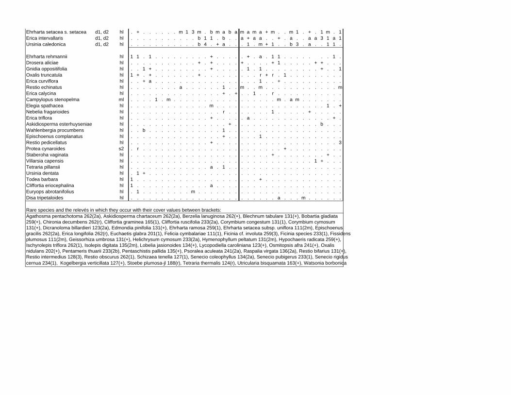
Ehrharta setacea s. setacea d1, d2 hl . + . . . . . . m 1 3 m . b m a b a m a m a + m . . m 1 . + . 1 m . 1Erica intervallaris d1, d2 hl . . . . . . . . . . . b 1 1 . b . . a + a a . . + . a . . a a 3 1 a 1Ursinia caledonica d1, d2 hl . . . . . . . . . . . b 4 . + a . . . 1 . m + 1 . . b 3 . a . . 1 1 .
Ehrharta rehmannii hl 1 1 . 1 . . . . . . . . . + . . . . . + . a . 1 1 . . . . . . . 1 .Drosera aliciae hl . . . . . . . . . . . + . + . . . . + . . . . + 1 . . . . . + + . . .Gnidia oppositifolia hl . . 1 + . . . . . . . . . + . . . . . 1 . 1 . . . . . . . . . + . . 1Oxalis truncatula hl 1 + . + . . . . . . . + . . . . . . . . . r + r . 1 . . . . . . . . .Erica curviflora hl . . + a . . . . . . . . . . . . . . . . . 1 . . + . . . . . . . . . .Restio echinatus hl . . . . . . . . a . . . . . . 1 . . m . . m . . . . . . . . . . . . mErica calycina hl . . . . . . . . . . . . . . . + . + . . 1 . . r . . . . . . . . . . .Campylopus stenopelma ml . . . . 1 . m . . . . . . . . . . . . . . . . . m . a m . . . . . . .Elegia spathacea hl . . . . . . . . . . . . . m . . . . . . . . . . . . . . . . . . 1 . +Nebelia fragarioides hl . . . . . . . . . . . . . . . r . . . . . . . 1 . . . . . + . . . . .Erica triflora hl . . . . . . . . . . . . . + . . . . . a . . . . . . . . . . . . . + .Askidiosperma esterhuyseniae hl . . . . . . . . . . . . . . . . + . . . . . . . . . . . . . . b . . .Wahlenbergia procumbens hl . . b . . . . . . . . . . . . 1 . . . . . . . . . . . . . . . . . . .Epischoenus complanatus hl . . . . . . . . . . . . . . . + . . . . . 1 . . . . . . . . . . . . .Restio pedicellatus hl . . . . . . . . . . . . . + . . . . . . . . . . . . . . . . . . . . 3Protea cynaroides s2 . r . . . . . . . . . . . . . . . . . . . . . . . + . . . . . . . . .Staberoha vaginata hl . . . . . . . . . . . . . . . . . . . . . . . + . . . . . . . . + . .Villarsia capensis hl . . . . . . . . . . . . . . . . . . . . . . . . . . . . . . 1 + . . .Tetraria pillansii hl . . . . . . . . . . . . . a . 1 . . . . . . . . . . . . . . . . . . .Ursinia dentata hl . 1 + . . . . . . . . . . . . . . . . . . . . . . . . . . . . . . . .Todea barbara hl 1 . . . . . . . . . . . . . . . . . . . . + . . . . . . . . . . . . .Cliffortia eriocephalina hl 1 . . . . . . . . . . . . a . . . . . . . . . . . . . . . . . . . . .Euryops abrotanifolius hl . 1 . . . . . . . . m . . . . . . . . . . . . . . . . . . . . . . . .Disa tripetaloides hl . . . . . . . . . . . . . . . . . . . . . . . . a . . . m . . . . . .
cernua 234(1), Kogelbergia verticillata 127(+), Stoebe plumosa-jl 188(r), Tetraria thermalis 124(r), Utricularia bisquamata 163(+), Watsonia borbonica
Agathosma pentachotoma 262(2a), Askidiosperma chartaceum 262(2a), Berzelia lanuginosa 262(+), Blechnum tabulare 131(+), Bobartia gladiata 259(+), Chironia decumbens 262(r), Cliffortia graminea 165(1), Cliffortia ruscifolia 233(2a), Corymbium congestum 131(1), Corymbium cymosum 131(+), Dicranoloma billardieri 123(2a), Edmondia pinifolia 131(+), Ehrharta ramosa 259(1), Ehrharta setacea subsp. uniflora 111(2m), Epischoenus gracilis 262(2a), Erica longifolia 262(r), Euchaetis glabra 201(1), Felicia cymbalariae 111(1), Ficinia cf. involuta 259(3), Ficinia species 233(1), Fissidens plumosus 111(2m), Geissorhiza umbrosa 131(+), Helichrysum cymosum 233(2a), Hymenophyllum peltatum 131(2m), Hypochaeris radicata 259(+), Ischyrolepis triflora 262(1), Isolepis digitata 135(2m), Lobelia jasionoides 134(+), Lycopodiella caroliniana 123(+), Osmitopsis afra 241(+), Oxalis nidulans 202(+), Pentameris thuarii 233(2b), Pentaschistis pallida 135(+), Psoralea aculeata 241(2a), Raspalia virgata 136(2a), Restio bifarius 131(+), Restio intermedius 128(3), Restio obscurus 262(1), Schizaea tenella 127(1), Senecio coleophyllus 134(2a), Senecio pubigerus 233(1), Senecio rigidus
Rare species and the relevés in which they occur with their cover values between brackets:
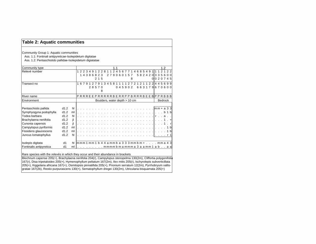
Community Group 1: Aquatic communities Ass. 1.1: Fontinali antipyreticae-Isolepidetum digitatae Ass. 1.2: Pentaschistido pallidae-Isolepidetum digiatatae
Community typeRelevé number 1 2
124
33
48
96
182
221
235
8 12
17
29
40
56
60
71
75
178
4 65
88
52
44
92
100
130
132
250
167
204
205
Transect no 1 6 7 9 12
28
75
97
108
3 4 5 8 10
14
15
19
20
72
2 16
26
13
11
27
29
46
47
50
66
90
90
River name P R R R E E P R R R R R B E R R P P B R R R B E E B P P R B B BEnvironment
Pentaschistis pallida d1.2 hl . . . . . . . . . . . . . . . . . . . . . . . . . . m m + a 3 3Symphyogyna podophylla d1.2 ml . . . . . . . . . . . . . . . . . . . . . . . . . . . . . b 1 bTodea barbara d1.2 hl . . . . . . . . . . . . . . . . . . . . . . . . . . r . . a . .Brachylaena neriifolia d1.2 jl . . . . . . . . . . . . . . . . . . . . . . . . . . . . . 1 . +Cunonia capensis d1.2 jl . . . . . . . . . . . . . . . . . . . . . . . . . . . . . 1 . rCampylopus pyriformis d1.2 ml . . . . . . . . . . . . . . . . . . . . . . . . . . . . . . 1 bFissidens glaucescens d1.2 ml . . . . . . . . . . . . . . . . . . . . . . . . . . . . . . 1 bJuncus lomatophyllus d1.2 hl . . . . . . . . . . . . . . . . . . . . . . . . . . . . . . r 1
Isolepis digitata d1 hl m m m 1 m m 1 b 4 4 a m m b a 3 3 3 m m b m + . . . . m m a 4 3Fontinalis antipyretica d1 ml . . . . . . . . . m m m m b m a m m m a 3 a a m m 1 a b . . a a
Table 2: Aquatic communities
Rare species with the relevés in which they occur and their abundance in bracketsBlechnum capense 205(+), Brachylaena neriifolia 204(r), Campylopus stenopelma 130(2m), Cliffortia polygonifolia 167(r), Disa tripetaloides 205(+), Hymenophyllum peltatum 167(2m), Ilex mitis 205(r), Ischyrolepis subverticillata 205(+), Kiggelaria africana 167(+), Osmitopsis pinnatifida 205(+), Prionium serratum 12(2m), Pyrrhobryum vallis-gratae 167(2b), Restio purpurascens 130(+), Sematophyllum dregei 130(2m), Utricularia bisquamata 205(+)
1.1 1.2
Boulders, water depth > 10 cm Bedrock

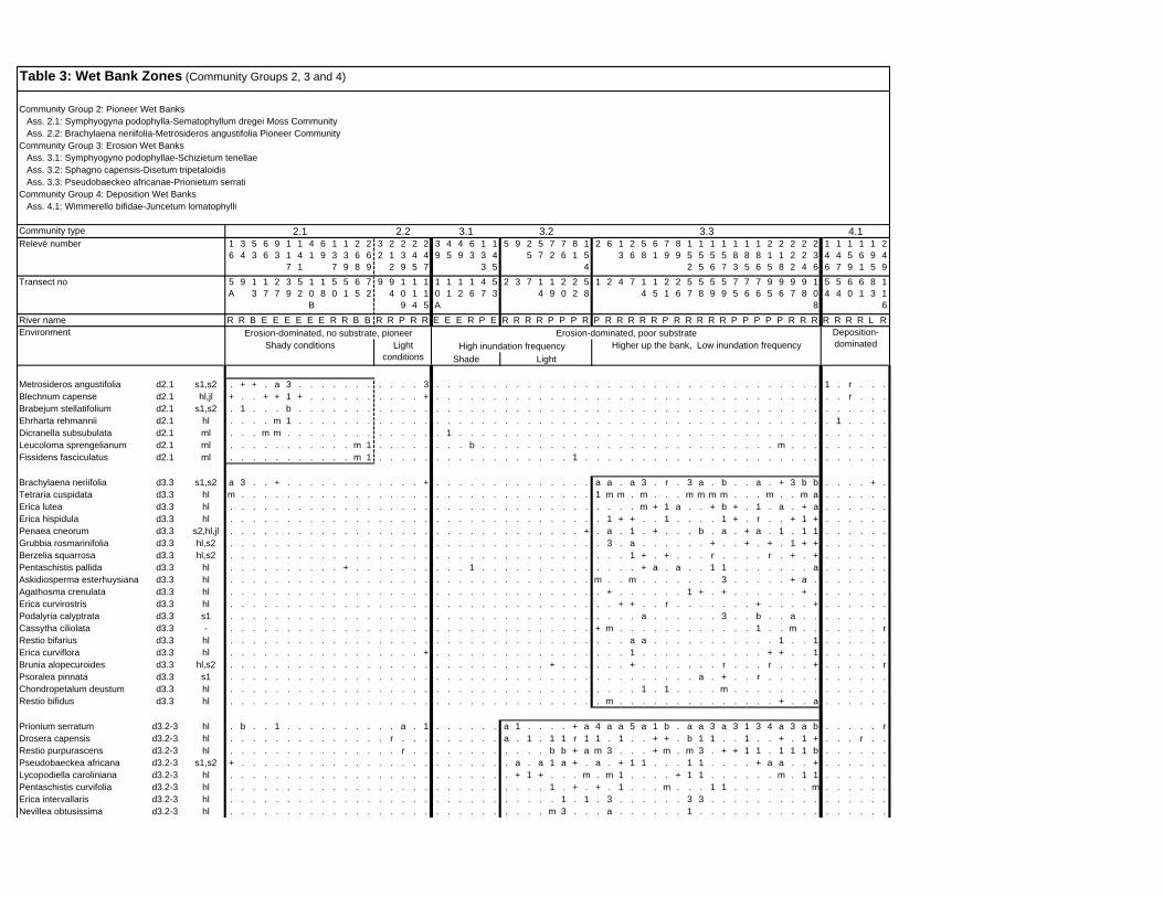
Community Group 2: Pioneer Wet Banks Ass. 2.1: Symphyogyna podophylla-Sematophyllum dregei Moss Community Ass. 2.2: Brachylaena neriifolia-Metrosideros angustifolia Pioneer CommunityCommunity Group 3: Erosion Wet Banks Ass. 3.1: Symphyogyno podophyllae-Schizietum tenellae Ass. 3.2: Sphagno capensis-Disetum tripetaloidis Ass. 3.3: Pseudobaeckeo africanae-Prionietum serratiCommunity Group 4: Deposition Wet Banks Ass. 4.1: Wimmerello bifidae-Juncetum lomatophylli
Community typeRelevé number 1
634
53
66
93
117
141
41
69
137
139
268
269
32
212
239
245
247
39
45
49
63
133
145
5 9 25
57
72
76
81
154
2 6 13
26
58
61
79
89
152
155
156
157
183
185
186
215
218
222
224
236
146
147
159
161
195
249
Transect no 5A
9 13
17
27
39
52
10B
18
50
51
65
72
9 94
109
114
115
10A
11
12
16
47
53
2 3 7 14
19
20
22
58
1 2 4 7 14
15
21
26
57
58
59
59
75
76
76
95
96
97
98
108
54
54
60
61
83
116
River name R R B E E E E E E R R B B R R P R R E E E R P E R R R R P P P R P R R R R R P R R R R R P P P P P R R R R R R R L R
Metrosideros angustifolia d2.1 s1,s2 . + + . a 3 . . . . . . . . . . . 3 . . . . . . . . . . . . . . . . . . . . . . . . . . . . . . . . . . 1 . r . . .Blechnum capense d2.1 hl,jl + . . + + 1 + . . . . . . . . . . + . . . . . . . . . . . . . . . . . . . . . . . . . . . . . . . . . . . . r . . .Brabejum stellatifolium d2.1 s1,s2 . 1 . . . b . . . . . . . . . . . . . . . . . . . . . . . . . . . . . . . . . . . . . . . . . . . . . . . . . . . .Ehrharta rehmannii d2.1 hl . . . . m 1 . . . . . . . . . . . . . . . . . . . . . . . . . . . . . . . . . . . . . . . . . . . . . . . 1 . . . .Dicranella subsubulata d2.1 ml . . . m m . . . . . . . . . . . . . . 1 . . . . . . . . . . . . . . . . . . . . . . . . . . . . . . . . . . . . . .Leucoloma sprengelianum d2.1 ml . . . . . . . . . . . m 1 . . . . . . . . b . . . . . . . . . . . . . . . . . . . . . . . . . . m . . . . . . . . .Fissidens fasciculatus d2.1 ml . . . . . . . . . . . m 1 . . . . . . . . . . . . . . . . . 1 . . . . . . . . . . . . . . . . . . . . . . . . . . .
Brachylaena neriifolia d3.3 s1,s2 a 3 . . + . . . . . . . . . . . . + . . . . . . . . . . . . . . a a . a 3 . r . 3 a . b . . a . + 3 b b . . . . + .Tetraria cuspidata d3.3 hl m . . . . . . . . . . . . . . . . . . . . . . . . . . . . . . . 1 m m . m . . . m m m m . . . m . . m a . . . . . .Erica lutea d3.3 hl . . . . . . . . . . . . . . . . . . . . . . . . . . . . . . . . . . . . m + 1 a . . + b + . 1 . a . + a . . . . . .Erica hispidula d3.3 hl . . . . . . . . . . . . . . . . . . . . . . . . . . . . . . . . . 1 + + . . 1 . . . . 1 + . r . . + 1 + . . . . . .Penaea cneorum d3.3 s2,hl,jl . . . . . . . . . . . . . . . . . . . . . . . . . . . . . . . + . a . 1 . + . . . b . a . + a . 1 . 1 1 . . . . . .Grubbia rosmarinifolia d3.3 hl,s2 . . . . . . . . . . . . . . . . . . . . . . . . . . . . . . . . . 3 . a . . . . . . + . . + . + . 1 + + . . . . . .Berzelia squarrosa d3.3 hl,s2 . . . . . . . . . . . . . . . . . . . . . . . . . . . . . . . . . . . 1 + . + . . . r . . . . r . + . + . . . . . .Pentaschistis pallida d3.3 hl . . . . . . . . . . + . . . . . . . . . . 1 . . . . . . . . . . . . . . + a . a . . 1 1 . . . . . . . a . . . . . .Askidiosperma esterhuysiana d3.3 hl . . . . . . . . . . . . . . . . . . . . . . . . . . . . . . . . m . . m . . . . . . . 3 . . . . . + a . . . . . . .Agathosma crenulata d3.3 hl . . . . . . . . . . . . . . . . . . . . . . . . . . . . . . . . . + . . . . . . 1 + . + . . . . . . + . . . . . . .Erica curvirostris d3.3 hl . . . . . . . . . . . . . . . . . . . . . . . . . . . . . . . . . . + + . . r . . . . . . . + . . . . + . . . . . .Podalyria calyptrata d3.3 s1 . . . . . . . . . . . . . . . . . . . . . . . . . . . . . . . . . . . . a . . . . . . 3 . . b . . a . . . . . . . .Cassytha ciliolata d3.3 - . . . . . . . . . . . . . . . . . . . . . . . . . . . . . . . . + m . . . . . . . . . . . . 1 . . m . . . . . . . rRestio bifarius d3.3 hl . . . . . . . . . . . . . . . . . . . . . . . . . . . . . . . . . . . a a . . . . . . . . . . . 1 . . 1 . . . . . .Erica curviflora d3.3 hl . . . . . . . . . . . . . . . . . + . . . . . . . . . . . . . . . . . 1 . . . . . . . . . . . + + . . 1 . . . . . .Brunia alopecuroides d3.3 hl,s2 . . . . . . . . . . . . . . . . . . . . . . . . . . . . + . . . . . . + . . . . . . . r . . . r . . . + . . . . . rPsoralea pinnata d3.3 s1 . . . . . . . . . . . . . . . . . . . . . . . . . . . . . . . . . . . . . . . . . a . + . . r . . . . . . . . . . .Chondropetalum deustum d3.3 hl . . . . . . . . . . . . . . . . . . . . . . . . . . . . . . . . . . . . 1 . 1 . . . . m . . . . . . . . . . . . . .Restio bifidus d3.3 hl . . . . . . . . . . . . . . . . . . . . . . . . . . . . . . . . . m . . . . . . . . . . . . . . + . . a . . . . . .
Prionium serratum d3.2-3 hl . b . . 1 . . . . . . . . . . a . 1 . . . . . . a 1 . . . . + a 4 a a 5 a 1 b . a a 3 a 3 1 3 4 a 3 a b . . . . . rDrosera capensis d3.2-3 hl . . . . . . . . . . . . . . r . . . . . . . . . a . 1 . 1 1 r 1 1 . 1 . . + + . b 1 1 . . 1 . . + . 1 + . . . r . .Restio purpurascens d3.2-3 hl . . . . . . . . . . . . . . . r . . . . . . . . . . . . b b + a m 3 . . . + m . m 3 . + + 1 1 . 1 1 1 b . . . . . .Pseudobaeckea africana d3.2-3 s1,s2 + . . . . . . . . . . . . . . . . . . . . . . . . a . a 1 a + . a . + 1 1 . . . 1 1 . . . . + a a . . + . . . . . .Lycopodiella caroliniana d3.2-3 hl . . . . . . . . . . . . . . . . . . . . . . . . . + 1 + . . . m . m 1 . . . . + 1 1 . . . . . . m . 1 1 . . . . . .Pentaschistis curvifolia d3.2-3 hl . . . . . . . . . . . . . . . . . . . . . . . . . . . . 1 . + . + . 1 . . . m . . . 1 1 . . . . . . . m . . . . . .Erica intervallaris d3.2-3 hl . . . . . . . . . . . . . . . . . . . . . . . . . . . . . 1 . 1 . 3 . . . . . . 3 3 . . . . . . . . . . . . . . . .Nevillea obtusissima d3.2-3 hl . . . . . . . . . . . . . . . . . . . . . . . . . . . . m 3 . . . a . . . . . . 1 . . . . . . . . . . . . . . . . .
4.13.3
Shade Light
Erosion-dominated, poor substrateHigh inundation frequency
3.2
Shady conditions
2.1 2.2 3.1
Environment
Table 3: Wet Bank Zones (Community Groups 2, 3 and 4)
Light conditions
Deposition-dominatedHigher up the bank, Low inundation frequency
Erosion-dominated, no substrate, pioneer
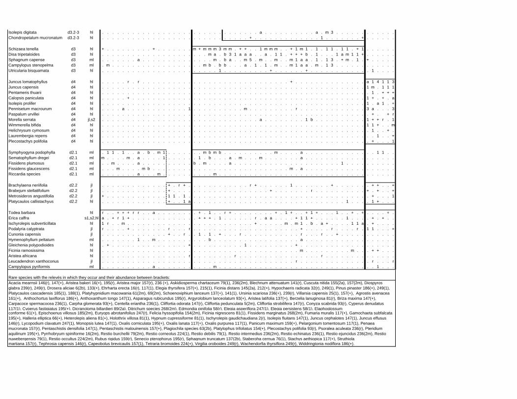
Isolepis digitata d3.2-3 hl . . . . . . . . . . . . . . . . . . . . . . . . . . . . . . . a . . . . . . . . . . a . m 3 . . . . . . . . . . . .Chondropetalum mucronatum d3.2-3 hl . . . . . . . . . . . . . . . . . . . . . . . . . . . . . + . . . . . . . . . . . . . 1 . . . . . . . + . . . . . .
Schizaea tenella d3 hl + . . . . . . . . . + . . . . . . . m + m m m 3 m m . + + . . 1 m m m . . + 1 m 1 . 1 . 1 1 . 1 1 . + 1 . . . . . .Disa tripetaloides d3 hl . . . . . . . . . . . . . . . . . . . . . m a . b 3 1 a a a . . a . 1 1 . + + + b . 1 . . . 1 a m 1 1 + . . . . . .Sphagnum capense d3 ml . . . . . . . a . . . . . . . . . . . . . . m . b a . . m 5 . m . . m . . m 1 a a . 1 . 1 3 . + m . 1 . + . . . . .Campylopus stenopelma d3 ml . m . . . . . . . . . . . . . . . . . . m b . b b . . . a . 1 . 1 . m . . m 1 a a . m . 1 3 . . . . . . . . . . . .Utricularia bisquamata d3 hl . . . . . . . . . . . . . . . . . . . . . . . 1 . . . . . . . . . + . . . . . . + . . . . . . . . . . . . 1 . . . .
Juncus lomatophyllus d4 hl . . . . . r . r . . . . . . . . . . . . . . . . . . . . . . . . . . . . . + . . . . . . . . . . . . . . a 1 4 1 1 3Juncus capensis d4 hl . . . . . . . . . . . . . . . . . . . . . . . . . . . . . . . . . . . . . . . . . . . . . . . . . . . . 1 m . 1 1 1Pentameris thuarii d4 hl . . . . . . . . . . . . . . . . . . . . . . . . . . . . . . . . . . . . . . . . . . . . . . . . . . . . . 1 . + + +Calopsis paniculata d4 hl . . . . . + . . . . . . . . . . . . . . . . . . . . . . . . . . . . . . . . . . . . . . . . . . . . . . 1 + . + . aIsolepis prolifer d4 hl . . . . . . . . . . . . . . . . . . . . . . . . . . . . . . . . . . . . . . . . . . . . . . . . . . . . 1 . a 1 . +Pennisetum macrourum d4 hl . . . . a . . . . . . . . . . . . 1 . . . . . . . . . . m . . . . . . . . . r . . . . . . . . . . . . . 3 a . . . 3Paspalum urvillei d4 hl . . . . . . . . . . . . . . . . . . . . . . . . . . . . . . . . . . . . . . . . . . . . . . . . . . . . . + . + rMorella serrata d4 jl,s2 . . . . . . . . . . . . . . . . . . . . . . . . . . . . . . . a . . . . . . . . 1 b . . . . . . . . . . 1 + + r . 1Wimmerella bifida d4 hl . . . . . . . . . . . . . . . . . . . . . . . . . . . . . . . . . . . . . . . . . . . . . . . . . . . . 1 1 + . . mHelichrysum cymosum d4 hl . . . . . . . . . . . . . . . . . . . . . . . . . . . . . . . . . . . . . . . . . . . . . . . . . . . . . 1 . . + .Laurembergia repens d4 hl . . . . . . . . . . . . . . . . . . . . . . . . . . . . . . . . . . . . . . . . . . . . . . . . . . . . . . 1 . . +Plecostachys polifolia d4 hl . . . . . . . . . . . . . . . . . . . . . . . . . . . . . . . . . . . . . . . . . . . . . . . . . . . . . + . . . 1
Symphyogyna podophylla d2.1 ml . 1 1 . 1 . . a . b . m 1 . . . . . . . m b m b . . . . . . . . . . m . . . . a . . . . . . . . . . . . . . 1 1 . .Sematophyllum dregei d2.1 ml m . . . . m . a . . . . 1 . . . . . . 1 . b . . . a . m . . . m . . . . . . . a . . . . . . . . . . . . . . . . . .Fissidens plumosus d2.1 ml . . m . . . . a . . . . . . . . . . b . m . . . . a . . . . . . . . . . . . . . . . . . . . . 1 . . . . . . . . . .Fissidens glaucescens d2.1 ml . . . m . . . . m b . . . . . . . . . . . . . . . . . . . . . . . . . . . m . a . . . . . . . . . . . . . . . . . .Riccardia species d2.1 ml . . . . . . . a . . . m . . . . . . . . . . m . . . . . . . . . . . . . . . . . . . . . . . . . . . . . . . . . . .
Brachylaena neriifolia d2.2 jl . . . . . . . . . . . . . + . r + . . . . . . . . . . . . r + . . . . . . 1 . . . . . . . + . . . . . . . + + . . +Brabejum stellatifolium d2.2 jl . . . . . . . . . . . . . + . . . . . . . . . . . . . . . . . . . + . . . . . . . r . . . . . . . . . . + . + . . +Metrosideros angustifolia d2.2 jl + . . . . . . . . . . . . 1 1 . 1 . . . . . . . . . . . . . . . . . . . . . . . . . . . . . . . . . . . . + . . . 1Platycaulos callistachyus d2.2 hl . . . . . . . . . . . . . + . . 1 a . . . . . . . . . . . . . . . . . . . . . . . . . . . . . . 1 . . . . 1 + . . .
Todea barbara hl r . . + + + r r . . a . . . . . . . . + . 1 . . r + . . . . . . . . + . 1 + . . + 1 + . . . 1 . . + . + . . . . + .Erica caffra s1,s2,hl a . + r 1 + . . . . . . . . . . . . . + + + . 1 . . . . . . r . a a . . . . + 1 1 + . . . . . . 1 . . . . + . + . .Ischyrolepis subverticillata hl 1 r . . m . . . . . . . . . . . . . . . . . . . . . . . . . + . . . . . m . m 1 . b . a + . . . . 1 1 a . + . . . .Podalyria calyptrata jl r . . . . + . . . . . . . r . . . r . . . . . . . . . . . . . . . . . . . . . + . . . . . r . . . . r . 1 1 . . . +Cunonia capensis jl . . . . . . . . . . . . . + . . r . . 1 . 1 . + . . . r . . . . . . . . . . . r . . . r . . + . . . . . . . . . . .Hymenophyllum peltatum ml . . . . . . . 1 . . m . . . . . . . . . . b . . . . . . . . . . . . . . . . . a . . . . . . . . . . . . . . . . . .Gleichenia polypodioides hl . + . . . . . . . . . . . . . . . + . . . . . . . . . . 1 . . . . . . . . . + . . . . . . . . . . . . . . . . . . .Ficinia ramosissima hl . . . . . . . . . . . . . . . . . . . . . . . . . . . . . . . . . . . . . . . m . . . . . . . . . m . . . + + . . .Aristea africana hl . . . . . . . . . . . . . . . . . r . . . . . . . . r . . . . . . . . . . . . . . . . r . . . . . . . . . . . . . .Leucadendron xanthoconus jl . . . . . . . . . . . . . . . . . . . . . . . . . . . . . . . . . . . . . . r . . . . . . . . . . . . . . r . . . rCampylopus pyriformis ml . . . . . . . . . . a . . . . . . . . . . . m . . . . . . . . . . . . . . . . . . . . . . . . . . . . . . . 1 . . .
martiana 157(r), Tephrosia capensis 146(r), Capeobolus brevicaulis 157(1), Tetraria bromoides 224(+), Virgilia oroboides 249(r), Wachendorfia thyrsiflora 249(r), Widdringtonia nodiflora 186(+).
Rare species with the relevés in which they occur and their abundance between brackets:Acacia mearnsii 146(r), 147(+), Aristea bakeri 16(+), 195(r), Aristea major 157(r), 236 (+), Askidiosperma chartaceum 79(1), 236(2m), Blechnum attenuatum 141(r), Cuscuta nitida 155(2a), 157(2m), Diospyros glabra 239(r), 249(r), Drosera aliciae 6(2b), 133(+), Ehrharta erecta 16(r), 117(1), Elegia thyrsifera 157(+), 215(1), Ficinia distans 145(2a), 212(+), Hypochaeris radicata 32(r), 249(1), Pinus pinaster 186(+), 249(1), Platycaulos cascadensis 185(1), 188(1), Platyhypnidium macowania 61(2m), 69(2m), Schoenoxiphium lanceum 137(+), 141(1), Ursinia scariosa 236(+), 239(r), Villarsia capensis 25(1), 157(+), Agrostis avenacea 161(+), Anthochortus laxiflorus 186(+), Anthoxanthum tongo 147(1), Asparagus rubicundus 195(r), Argyrolobium lanceolatum 93(+), Aristea latifolia 137(+), Berzelia lanuginosa 81(r), Briza maxima 147(+), Carpacoce spermacocea 236(1), Carpha glomerata 93(+), Centella eriantha 236(1), Cliffortia odorata 147(r), Cliffortia pedunculata 5(2m), Cliffortia strobilifera 147(r), Conyza scabrida 93(r), Cyperus denudatus 117(1), Cyperus fastigiatus 195(+), Dicranoloma billardieri 89(2a), Ditrichum species 268(2m), Edmondia pinifolia 58(r), Elegia asperiflora 247(1), Elegia persistens 58(1), Elaphoglossum conforme 61(+), Epischoenus villosus 185(2m), Euryops abrotanifolius 247(r), Felicia hyssopifolia 154(2m), Ficinia nigrescens 81(1), Fissidens marginatus 268(2m), Fumaria muralis 117(+), Gamochaeta subfalcata 195(+), Halleria elliptica 66(+), Heterolepis aliena 81(+), Holothrix villosa 81(1), Hypnum cupressiforme 81(1), Ischyrolepis gaudichaudiana 2(r), Isolepis fluitans 147(1), Juncus cephalotes 147(1), Juncus effusus 146(r), Lycopodium clavatum 247(1), Monopsis lutea 147(1), Oxalis corniculata 195(+), Oxalis lanata 117(+), Oxalis purpurea 117(1), Panicum maximum 159(+), Pelargonium tomentosum 117(1), Penaea mucronata 157(r), Pentaschistis densifolia 147(1), Pentaschistis malouinensis 157(+), Plagiochila species 63(2b), Platylophus trifoliatus 154(+), Plecostachys polifolia 93(r), Psoralea aculeata 236(r), Pteridium aquilinum 195(+), Pyrrhobryum spiniforme 16(2m), Restio burchellii 79(2m), Restio corneolus 224(1), Restio debilis 79(1), Restio intermedius 236(2m), Restio echinatus 236(1), Restio ejuncidus 236(2m), Restio nuwebergensis 79(1), Restio occultus 224(2m), Rubus rigidus 159(r), Senecio pterophorus 195(r), Sphagnum truncatum 137(2b), Staberoha cernua 76(1), Stachys aethiopica 117(+), Struthiola
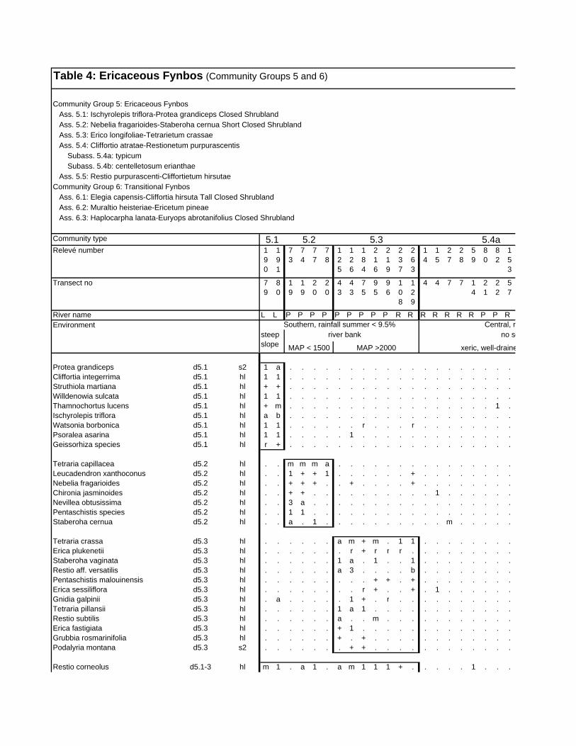
Community Group 5: Ericaceous Fynbos Ass. 5.1: Ischyrolepis triflora-Protea grandiceps Closed Shrubland Ass. 5.2: Nebelia fragarioides-Staberoha cernua Short Closed Shrubland Ass. 5.3: Erico longifoliae-Tetrarietum crassae Ass. 5.4: Cliffortio atratae-Restionetum purpurascentis Subass. 5.4a: typicum Subass. 5.4b: centelletosum erianthae Ass. 5.5: Restio purpurascenti-Cliffortietum hirsutaeCommunity Group 6: Transitional Fynbos Ass. 6.1: Elegia capensis-Cliffortia hirsuta Tall Closed Shrubland Ass. 6.2: Muraltio heisteriae-Ericetum pineae Ass. 6.3: Haplocarpha lanata-Euryops abrotanifolius Closed Shrubland
Community typeRelevé number 1
90
191
73
74
77
78
125
126
184
216
219
237
263
14
15
27
28
59
80
82
153
Transect no 79
80
19
19
20
20
43
43
75
95
96
108
129
4 4 7 7 14
21
22
57
River name L L P P P P P P P P P R R R R R R R P P R
Protea grandiceps d5.1 s2 1 a . . . . . . . . . . . . . . . . . . .Cliffortia integerrima d5.1 hl 1 1 . . . . . . . . . . . . . . . . . . .Struthiola martiana d5.1 hl + + . . . . . . . . . . . . . . . . . . .Willdenowia sulcata d5.1 hl 1 1 . . . . . . . . . . . . . . . . . . .Thamnochortus lucens d5.1 hl + m . . . . . . . . . . . . . . . . . 1 .Ischyrolepis triflora d5.1 hl a b . . . . . . . . . . . . . . . . . . .Watsonia borbonica d5.1 hl 1 1 . . . . . . r . . . r . . . . . . . .Psoralea asarina d5.1 hl 1 1 . . . . . 1 . . . . . . . . . . . . .Geissorhiza species d5.1 hl r + . . . . . . . . . . . . . . . . . . .
Tetraria capillacea d5.2 hl . . m m m a . . . . . . . . . . . . . . .Leucadendron xanthoconus d5.2 hl . . 1 + + 1 . . . . . . + . . . . . . . .Nebelia fragarioides d5.2 hl . . + + + . . + . . . . + . . . . . . . .Chironia jasminoides d5.2 hl . . + + . . . . . . . . . . 1 . . . . . .Nevillea obtusissima d5.2 hl . . 3 a . . . . . . . . . . . . . . . . .Pentaschistis species d5.2 hl . . 1 1 . . . . . . . . . . . . . . . . .Staberoha cernua d5.2 hl . . a . 1 . . . . . . . . . . m . . . . .
Tetraria crassa d5.3 hl . . . . . . a m + m . 1 1 . . . . . . . .Erica plukenetii d5.3 hl . . . . . . . r + r r r . . . . . . . . .Staberoha vaginata d5.3 hl . . . . . . 1 a . 1 . . 1 . . . . . . . .Restio aff. versatilis d5.3 hl . . . . . . a 3 . . . . b . . . . . . . .Pentaschistis malouinensis d5.3 hl . . . . . . . . . + + . + . . . . . . . .Erica sessiliflora d5.3 hl . . . . . . . . r + . . + . 1 . . . . . .Gnidia galpinii d5.3 hl . a . . . . . 1 + . r . . . . . . . . . .Tetraria pillansii d5.3 hl . . . . . . 1 a 1 . . . . . . . . . . . .Restio subtilis d5.3 hl . . . . . . a . . m . . . . . . . . . . .Erica fastigiata d5.3 hl . . . . . . + 1 . . . . . . . . . . . . .Grubbia rosmarinifolia d5.3 hl . . . . . . + . + . . . . . . . . . . . .Podalyria montana d5.3 s2 . . . . . . . + + . . . . . . . . . . . .
Restio corneolus d5.1-3 hl m 1 . a 1 . a m 1 1 1 + . . . . . 1 . . .
Table 4: Ericaceous Fynbos (Community Groups 5 and 6)
5.1 5.2 5.3 5.4a
Environment Southern, rainfall summer < 9.5% Central, rsteep slope
river bank no se
MAP < 1500 MAP >2000 xeric, well-draine
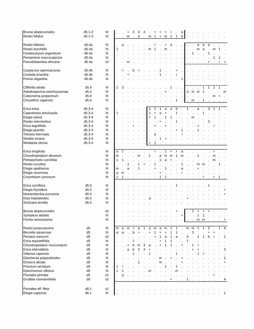
Brunia alopecuroides d5.1-3 hl . . + 3 4 4 . + + + r . a . . . . . . . .Restio bifidus d5.1-3 hl . . m . a . m 1 + m 1 1 b . . . . . . . .
Restio bifarius d5.4a hl . a . . . . . r . r a . . . . a a a . . .Restio burchellii d5.4a hl 1 . . . . . m 1 . m . . . . . m a . m 1 .Ceratocaryum argenteum d5.4a hl . . . . . . . . . . . . . . 1 . . 1 . . .Pentameris macrocalycina d5.4a hl . . . . . . . . . . . . . . . . . . 1 1 .Pseudobaeckea africana d5.4a s2 . . m . . . . . . . . . . . . . . + . r +
Carpacoce spermacocea d5.4b hl . + . b + . . . 1 . . + . . . . . . . . .Centella eriantha d5.4b hl . . + . . . . . 1 . . r . . . . . . . . .Ficinia oligantha d5.4b hl . . . . . . . . . . . . 1 . . . . . . . .
Cliffortia atrata d5.4 hl 1 3 . . . . . . . . 1 . . . . . 1 1 1 1 .Askidiosperma esterhuyseniae d5.4 hl . . . . . . . . . + . . . 3 m m 1 . . . mColeonema juniperinum d5.4 hl . . . . . . . . . . . . . . . . . . m + .Chrysithrix capensis d5.4 hl . . . . . . . . . . . 1 . . m . 1 . . . .
Erica lutea d5.3-4 hl . . . . . . 1 1 1 a a b . 1 . a . 3 1 1 .Capeobolus brevicaulis d5.3-4 hl 1 . . . . . 1 + a + . 1 . . . . 1 . . . .Elegia neesii d5.3-4 hl . . . . . . + 1 . 1 1 . . . m . . . . . .Restio intermedius d5.3-4 hl . . . . . . . . + . . 1 . . . . . 3 . . .Erica tegulifolia d5.3-4 hl . . . r . . . + . + . . . . . + . . r . .Elegia grandis d5.3-4 hl . . . . . . . . . . . + 1 . . 1 . . . . .Tetraria thermalis d5.3-4 hl . . . . . . . a . . . . r . . . . . . . .Stoebe incana d5.3-4 hl . . . . . . . . 1 + . . . . . . . . . . .Metalasia densa d5.3-4 hl . . . . . . + 1 . . . . . . . . . . . . .
Erica longifolia hl a 1 . . . . . r . 1 + r a . . . . . r . .Chondropetalum deustum hl m . . . m . 1 . a m m 1 m . . 1 . . m . .Pentaschistis curvifolia hl 1 1 . . . . . . 1 a + . . . . . . . m . .Restio occultus hl . . 1 . 1 + . 1 . . . . 1 . . m m . . 1 .Elegia spathacea hl m . a . 1 . . + . 1 . . a . . + . . . . .Elegia racemosa hl a m . . . . . . + . . . r . . . . . . . .Corymbium cymosum hl 1 1 . . . . . . 1 1 . . . . . . r . r 1 .
Erica curviflora d5.5 hl . . . . . . . . . . . 1 . . . . . 1 . . .Elegia thyrsifera d5.5 hl . . . . . . . . . . . . . . . . . . . . +Neesenbeckia punctoria d5.5 hl . . . . . . . . . . . . . . . . . . . . +Disa tripetaloides d5.5 hl . . . . . . a . . . . . . + . . . . . . .Schizaea tenella d5.5 hl . . . . . . . . . . . . . . . . . . . . .
Brunia alopecuroides s2 . . . . . . . . . . . + . . 1 + + + . . .Sympieza labialis hl . . . . . . . . . . . . + . . 1 1 . . . .Ficinia ramosissima hl . . . . . . . . . . . . . . . m m . . . +
Restio purpurascens d5 hl m a m + a 1 a m a m 1 1 . m m 1 1 3 . 1 4Berzelia squarrosa d5 hl a a . b + . + 1 + + 1 1 . . 3 . . + + . .Penaea cneorum d5 s2 . . . . . . . + 1 a 1 a . 4 . 1 1 b r . 1Erica equisetifolia d5 hl . . . 1 . . . . + 1 1 . . 1 . . . . . . .Chondropetalum mucronatum d5 hl . . + b m 3 a . + 1 1 . + . 1 + . . . . .Erica intervallaris d5 hl . . a b 3 3 + . . . . . . . + + . . . . 3Villarsia capensis d5 hl . . . 1 . . 1 . . . . 1 . . . 1 + . . . .Gleichenia polypodioides d5 hl . . . . . . . . m . + . + . . . . . . . 1Drosera aliciae d5 hl . . . . 1 . . . m . . . + . . . . . . . +Prionium serratum d5 hl 1 + . . . . . . . 1 . 1 . . . . . . . . .Epischoenus villosus d5 hl 1 1 . . . . m . . . . m . . . . . . . . .Psoralea pinnata d5 s1 . a . . . . . . . . . . . . . . . . r . .Grubbia rosmarinifolia d5 s2 . . . . . . . . . . + . . 1 . . . . . . 4
Psoralea aff. fleta d6.1 s1 . . . . . . . . . . . . . . . . . . . . .Elegia capensis d6.1 hl . . . . . . . . . . . . . . . . . . . . 1
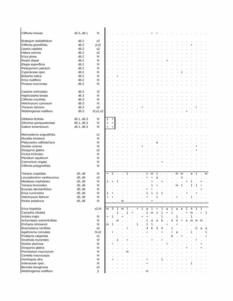
Cliffortia hirsuta d5.5, d6.1 hl . . . . . . . . . r r . . . . . . . . . .
Brabejum stellatifolium d6.2 s2 . . . . . . . . . . . . . . . . . . . . .Cliffortia grandifolia d6.2 jl,s2 . . . . . . . . . . . . . . . . . + . . .Liparia capitata d6.2 s2 . . . . . . . . . . . . . . . . . . . . .Hakea sericea d6.2 s2 . . . . . . . . . . . . . . . . . . . . .Erica pinea d6.2 hl . . . . . . . . . . . . . . . . . . . . .Restio dispar d6.2 hl . . . . . . . . . . . . + . . . . . . . .Elegia asperiflora d6.2 hl . . . . . . . . . . . . . . . . . . . . .Pelargonium patulum d6.2 hl . . . . . . . . . . . . . . . . . . . . .Cyperaceae spec. d6.2 hl . . . . . . . . . . . . . . . 1 . . . . .Bobartia indica d6.2 hl . . + . . . . . . . . . . . . . . . . . .Erica nudiflora d6.2 hl . . . . . . . . . . . . . . . . . . . . .Penaea mucronata d6.2 hl . . . . . . . . . . . . . . . . . . . . .
Cassine schinoides d6.3 t3 . . . . . . . . . . . . . . . . . . . . .Haplocarpha lanata d6.3 hl . . . . . . . . . . . . . . . . . . . . .Cliffortia ruscifolia d6.3 hl . . . . . . . . . . . . . . . . . . . . .Helichrysum cymosum d6.3 hl . . . . . . . . . . . . . . . . . . . . .Thesium strictum d6.3 s2 . . . . . . . r . . . . . . . . . . r . .Widdringtonia nodiflora d6.3 t3,s1,s2 . . . . . . . . . . . . . . . . + . . . .
Gibbaria ilicifolia d5.1, d6.3 hl 1 + . . . . . . . . . . . . . . . . . . .Othonna quinquedentata d5.1, d6.3 hl + + . . . . . . . . . . . . . . . . . . .Galium tomentosum d5.1, d6.3 hl + + . . . . . . . . . . . . . . . . . . .
Metrosideros angustifolia s1 . . . . . . . . . . . . . . . . . . . . .Muraltia heisteria hl . . . . . . . . . . . . . . . . . . . . .Platycaulos callistachyus hl . . . . . . . . . . a . . . . . . . . . .Stoebe cinerea hl . . . . . . . + . . . . . . . . . . + . .Diospyros glabra s2 . . . . . . . . . . . . . . . . . . + . .Ficinia trichodes hl . . . . . . . . . . . . . . . . . . . . .Pteridium aquilinum hl . . . . . . . . . . . . . . . . . . . . .Cannomois virgata hl . . . . . . . . . . . + . . . . . . . . .Cliffortia polygonifolia hl . . . . . . . . . . . . . . . . . . . . .
Tetraria cuspidata d5, d6 hl + 1 . . 1 . . . 1 m 1 . . . m m . a 1 . mLeucadendron xanthoconus d5, d6 s2 . . . . . . . . + + a . . . . 4 . . . . .Metalasia cephalotes d5, d6 hl 1 + 1 . . . . . . + . + . . . . + 1 . + .Tetraria bromoides d5, d6 hl . . . . . . . . . 1 + . . . m 1 . 1 1 r .Euryops abrotanifolius d5, d6 hl . . . . . . . . + r . . . . . . . . . + .Erica curvirostris d5, d6 hl 1 + . . . . . . 1 1 1 1 . . . . + . + . .Helichrysum felinum d5, d6 hl + r . . . . . . + . 1 . . . + . . 1 . . .Restio perplexus d5, d6 hl . . . m . . . . . + . . . . . . . . . . .
Erica hispidula s2,hl m 3 1 m 1 . + 1 a 1 + 1 a 1 a a 1 4 1 1 .Cassytha ciliolata - . . 1 . 1 + . . 1 m 1 1 + 1 . . + m . r 1Aristea major hl + 1 . + . . . + + . . 1 . . 1 . . 1 . . .Ischyrolepis subverticillata hl . . m . . . . . 1 a a b . 4 4 + a m m m .Ehrharta rehmannii hl m 1 . . . . 1 . 1 1 . . + . + . . . . . .Brachylaena neriifolia s2 . . . . + . . . 4 b 3 4 . 1 . . . . b a aAgathosma crenulata hl,s2 . + . . . . . . r . . + . + a . . 1 . . 1Podalyria calyptrata s1 . . . . . . . . . . . . . b . + . . . . rStruthiola myrsinites hl . . 1 . + . . . . + . r . . . . . . r . .Stoebe plumosa hl . + . . . . . . . . . . + . . . . . . + .Diospyros glabra hl . . . . . . . . . . . . . . . . + . . + .Pennisetum macrourum hl . . . . m . . . . . . . . . . . . . . . .Centella macrocarpa hl . . . . . . . . . . . . . . . . . . . . .Osmitopsis afra hl . + . . . . . . + . . 1 . . . . . . . . .Asteraceae spec. hl . . . . . . . . + . . . . . . . . 1 . . .Berzelia lanuginosa s2 . . . . . . . . . . . . . . . . . . . . .Widdringtonia nodiflora jl . . . . . . . . m . . . . . . . . . . . .
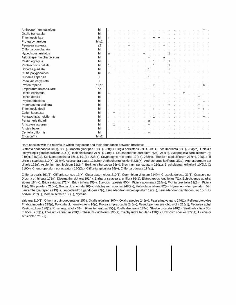
Anthospermum galioides hl . . . . . . . . . . . . . . . . . . . + .Oxalis truncatula hl . . . . . . . . . . . r . . . . . . . . .Tritoniopsis lata hl r . . . . . . . . + + . . . . . . . . . .Protea cynaroides hl,s2 . . . . . . . . . . . . . . . . . . . . .Psoralea aculeata s2 . . . . + . . . . . . + . . . . . . . . .Cliffortia complanata hl . . . . . . . . r . . . . . . . . . . .Hypodiscus aristatus hl a . . . . . . + . . . . 1 . . . . . . . .Askidiosperma chartaceum hl . . . . . . . . + . . a . . . . . . . . .Restio egregius hl . . . . . . . . . 1 . . 1 . . . . . . . .Pentaschistis pallida hl 1 . . . . . . . . 1 . . 1 . . . . . . . .Bobartia gladiata hl . + . . . . . . 1 . . . + . . + . . . . .Clutia polygonoides hl r . . . . . . . . . . . + . . + . . . . .Cunonia capensis jl . . . . . . . . 1 . r . . . . . . . . . .Podalyria calyptrata jl . . . . . . . . . . . + . . + . . . . . .Protea repens h1,s2 . . . . . . . . . r . . . . . . . . . a .Empleurum unicapsulare s2 . . . . . . . . + . . . . . . . . . . . .Restio echinatus hl 1 . . . . . . . . . . 1 . . . m . . . . .Restio debilis hl . . . . . . . . . + . . . . . . . . m . .Phylica ericoides hl . . . . . . . . . . . . . . . . . . 1 .Phaenocoma prolifera hl . . . . . . . . . . . . + . . . . . + . .Tritoniopsis dodii hl . . . . . . . . . r . . . . . . . . + r .Cullumia setosa hl . + . . . . . . . . . . . . . . . . . . .Pentaschistis holciformis hl . . . . . . . . . 1 . . . . . . . . . + .Pentameris thuarii hl . . . . . . . . a . . . . . . . . . . . .Anaxeton asperum hl . 1 . . . . . . + . . . . . . . . . . . .Aristea bakeri hl . . . . 1 . . . . . . . r . . . . . . . .Centella difformis hl . . . . . . . . + . . . . . . . . . . . .Erica caffra hl,s2 . . . . . . . . . . . . . . . . . . . . .
Cliffortia ovalis 191(1), Cliffortia sericea 11(+), Clutia alaternoides 210(1), Corymbium villosum 214(+), Crassula dejecta 31(1), Crassula nudDiosma cf. hirsuta 172(r), Diosma thyrsiphora 191(r), Ehrharta setacea s. uniflora 91(1), Elytropappus longifolius 7(1), Epischoenus quadransitiens 184(+), Erica strigosa 172(+), Erica triflora 85(+), Euryops rupestris 80(+), Ficinia acuminata 214(+), Ficinia brevifolia 31(2m), Ficinia 11(r), Glia prolifera 210(+), Gnidia cf. anomala 36(+), Helichrysum species 248(2a), Heterolepis aliena 82(+), Hymenophyllum peltatum 59(2Laurembergia repens 213(+), Leucadendron gandogeri 77(r), Leucadendron microcephalum 190(+), Leucadendron xanthoconus-jl 15(r), Lobodkinii 263(+), Morella serrata 153(+), Myrsine
africana 210(1), Othonna quinquedentatus 15(r), Oxalis nidulans 36(+), Oxalis species 246(+), Passerina vulgaris 246(1), Pellaea pteroides Phylica imberbis 225(r), Polygala cf. nematocaulis 10(r), Protea amplexicaulis 246(+), Pseudopentameris obtusifolia 216(1), Psoralea aphylRestio stokoei 190(1), Rhus angustifolia 31(r), Rhus tomentosa 35(r), Roella dregeana 184(r), Stoebe prostata 246(1), Struthiola ciliata 36(+fruticosus 85(1), Thesium carinatum 238(1), Thesium viridifolium 190(+), Trachyandra tabularis 190(+), Unknown species 172(1), Ursinia quschlechteri 216(+).
Rare species with the relevés in which they occur and their abundance between brackets:Cliffortia dodecandra 84(1), 85(+), Drosera glabripes 158(+), 220(+), Elegia persistens 27(1), 28(1), Erica imbricata 85(+), 263(2a), Gnidia oIschyrolepis gaudichaudiana 214(+), Isolepis fluitans 217(+), 240(+), Leucadendron laureolum 7(2a), 246(+), Lycopodiella carolinianum 7(+240(r), 246(2a), Schizaea pectinata 15(1), 191(1), 238(+), Scyphogyne micrantha 172(+), 238(4), Thesium capituliflorum 217(+), 220(1), ThUrsinia scariosa 210(+), 237(+), Adenandra acuta 126(2m), Anthochortus ecklonii 225(+), Anthochortus laxiflorus 3(2a), Anthospermum aetciliaris 172(r), Asplenium aethiopicum 31(2m), Berkheya herbacea 36(+), Blechnum punctulatum 210(1), Brachylaena neriifolia-jl 10(2b), Ca210(+), Chondropetalum ebracteatum 190(2a), Cliffortia apiculata 59(+), Cliffortia odorata 184(1),
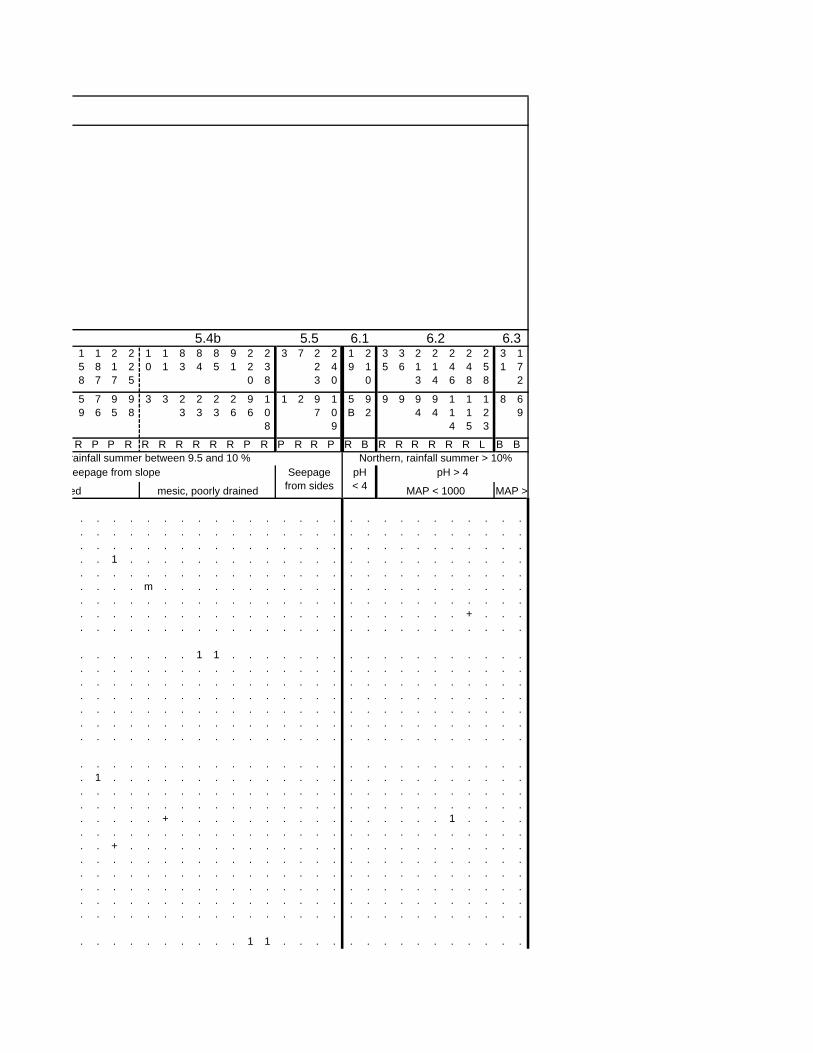
158
187
217
225
10
11
83
84
85
91
220
238
3 7 223
240
19
210
35
36
213
214
246
248
258
31
172
59
76
95
98
3 3 23
23
23
26
96
108
1 2 97
109
5B
92
9 9 94
94
114
115
123
8 69
R P P R R R R R R R P R P R R P R B R R R R R R L B B
. . . . . . . . . . . . . . . . . . . . . . . . . . .
. . . . . . . . . . . . . . . . . . . . . . . . . . .
. . . . . . . . . . . . . . . . . . . . . . . . . . .
. . 1 . . . . . . . . . . . . . . . . . . . . . . . .
. . . . . . . . . . . . . . . . . . . . . . . . . . .
. . . . m . . . . . . . . . . . . . . . . . . . . . .
. . . . . . . . . . . . . . . . . . . . . . . . . . .
. . . . . . . . . . . . . . . . . . . . . . . + . . .
. . . . . . . . . . . . . . . . . . . . . . . . . . .
. . . . . . . 1 1 . . . . . . . . . . . . . . . . . .
. . . . . . . . . . . . . . . . . . . . . . . . . . .
. . . . . . . . . . . . . . . . . . . . . . . . . . .
. . . . . . . . . . . . . . . . . . . . . . . . . . .
. . . . . . . . . . . . . . . . . . . . . . . . . . .
. . . . . . . . . . . . . . . . . . . . . . . . . . .
. . . . . . . . . . . . . . . . . . . . . . . . . . .
. . . . . . . . . . . . . . . . . . . . . . . . . . .
. 1 . . . . . . . . . . . . . . . . . . . . . . . . .
. . . . . . . . . . . . . . . . . . . . . . . . . . .
. . . . . . . . . . . . . . . . . . . . . . . . . . .
. . . . . + . . . . . . . . . . . . . . . . 1 . . . .
. . . . . . . . . . . . . . . . . . . . . . . . . . .
. . + . . . . . . . . . . . . . . . . . . . . . . . .
. . . . . . . . . . . . . . . . . . . . . . . . . . .
. . . . . . . . . . . . . . . . . . . . . . . . . . .
. . . . . . . . . . . . . . . . . . . . . . . . . . .
. . . . . . . . . . . . . . . . . . . . . . . . . . .
. . . . . . . . . . . . . . . . . . . . . . . . . . .
. . . . . . . . . . 1 1 . . . . . . . . . . . . . . .
5.4b 5.5 6.1 6.2 6.3
rainfall summer between 9.5 and 10 % Northern, rainfall summer > 10%eepage from slope Seepage
from sidespH < 4
pH > 4
MAP < 1000 MAP >ed mesic, poorly drained
. . . . . . . . . . . . . . . . . . . . . . . . . . .
. . . . . . . . . . . . . . . . . . . . . . . . . . .
b . . b . . . 1 . . . 1 . . . . . . . . 1 . 1 . . . .. . . 1 . . . . . . + . . . . . . . . . . . . . . . .. a 1 . . . . . . . . . . . . . . . . . . . . . . . .. . a + . . . . . . . . . . . . . . . . . . . . . . .. 1 . . . . . . . . . . . . a . . . . . . . . . . . .
. . . . . 1 r 1 + m 1 . . . . . . . . . . . . . . . .
. . . . m . + 3 a 1 . . . . . . . . . . . . . . . . 1
. . . . . . m 1 m . 1 . . . . . . . . . . . . . . . .
+ . 1 1 . + . r . 1 1 . . . . a . . . . . 1 1 . . . .1 . . . m a . . . . 1 . a . . . . . . . . . . . . . .. . a . . . . . . 1 . . . . . . . . . . . . . . . . .. . . . . . . + . . . 1 . . . . . . . . . . . . . . .
1 b . 1 . . . . . . 1 . + . . b . . . . . . . . . . .. . . r . 1 . . a . 1 . . . . . . . . . . . . . . . .1 . . . . . . . . . m . . 1 . . . . . . . . . . . . .. . . . a . . . . m . a . . . 1 . . . . . . . . . . .. . . . . . . . . . 1 . . . . . . . . . . . . . . . .. . . + . . . . . . . 1 . . . . . . . . . . . . . . .r . . + . . . . . . . . . . . . . . . . . . . . . . .. . . . . . . . . . . r . . . . . . . . . . . . . . .. . . . . . . . + . . . . . . . . . . . . . . . . . .
. . a . . . . . . . + . . . . + . . . . . . . . . . .1 . . 1 . . . . . . m . . . . . . . . . . . . . . . .. . . . . 1 . 1 . . . . . . . . . . . . . . . . . . .. . 1 . . . . . . . a . . . . . . . . . . . . . . . .. . . . . . . . . . + . . . . . . . . . . . . . . . .. + . . . . . . . . 1 1 . . . . . . . . . . . . . . .. . . + . r . + + . 1 . . . . r . . . . . + . . . . 1
. . . . . . . . . . . 1 1 . + r . . . . . . . . . . .
. . . . . . . . . m . . b . . 1 . . . . . . . . . . .
. . . . . . . . . . . . . a a . . . . . . . . . . . .
. . . . . . . . . . . . . . b + . . . . . . . . . . .
. . . . . . . . . . . . m . m . . . . . . . . . . . .
. . + . . . . . . . + . + + 1 . . . . . . . . . . . .
. . 3 + . . . . . . 1 . 1 . . 1 . . . . . . . + . . .
. . . . . . . . . 3 . . . . 4 . . . . . . . . . . . .
. . a 3 a a 1 4 b a . . b a a a . . m . . . . . a . .1 . r + b + . . . + . + a + 1 a . . . . . . . . . . .a . a a . 1 . + . + + . 1 1 1 a . . . . . . . . . . .. 3 . . . 1 . + . . a . . 1 . + . . . . . . . . . . .1 . . . . . . . . . . 1 m . 1 . . . . . . . . . . . .. . . . . . . 1 1 . . 1 . m . . . . . . . . . . . . .. . . 1 + . . . . . a . + . 1 . . . . . . . . . . . .a + . . . . + . 1 . . . . . 1 1 . . . . . . . . . . .. . . . . . . + . . . . . 1 + . . . . . . . . . . . .. . . . . . . . . . . . b 1 . . . . . . . . . . . . .. . . . . . . . . . . 1 . . . 1 . . . . . . . . . . .r . . . a . . . . . . . r . . . . . . . . . . . . . .. . . . . . . . . . . . . . b . . . . . . . . . . . .
. . . . . . . . . . . . . . . . a b . . . . . . . . .
. . . . . . . . . . . . . . . . 1 b . . . . . . . . .
. . . . . . . . . . . . 3 a b a 5 5 . . . . . . . . .
. . . . . . . . . . . . . . . . . . . . . a a b 1 . .
. . . . . . . . . . . r . . . . . . a . . . a 1 1 . .
. . . . . . . . . . . . . . . . . . . . . a + + . . .
. . . . . . . . . . . . . . . . . . . . . + r + . . .
. . . . . . . . . . . . . . . . . . . . . 4 a b 1 . .
. . . . . . . . . . . . . . . . . . . . 1 1 1 b . . .
. . . . . . . . . . . . . . . . . . 1 . + . + . + . .
. . . . . . . . . . . . . . . . . . . . . + 1 + . . .
. . . . . . . . . . . . . . . . . . . + . 1 + . . . .
. . . . . . . . . . . . . . . . . . 1 . . + . + . . .
. . . . . . . . . . . . . . . . . . . a . . . 1 . . .
. . . . . . . . . . . . . . . . . . . a . . . 1 . . .
. . . . . . . . . . . . . . . . . . . . . . . . . a r
. . . . . . . . . . . . . . . . . . . . . . . . . 1 +
. . . . . . . . . . . . . . . . . . . . . . . . . 1 +
. . . . . . . . . . . . . . . . . . . . . . . . . 1 1
. . . . . . . . . r . . . . . . . . . . . . 1 . . + +a . . . . + . . . . . . . . . . . . . . . . . . . r +
. . . . . . . + . 1 . . . . . . . . . . . . . . . 1 +
. . . . . . . . . . . . . . . . . . . . . . . . . 1 r
. . . . . . . . . 1 . . . . . . . 1 . . . . . . . . +
. . . . . . . . . . . . . . . . . b b . 3 a . . b a +
. . . . . . . . . + . . . . . . . . + 1 . + + + . r +
. . . . . . . . . . . . . . . . b . . . 3 . a a 3 . .
. . . . . . . . . . . . . . . . . + + 1 . + . . r . .
. . . . . . . . . . . . . . . . . . . . 1 + + . . a .
. . . . . 1 . . . . . . . . . . a m m . . . . . . . m
. . . . . . . . . . . . . . . . 1 . . . + a a . . . .
. . . . . . . . . . . 1 . . . . . . b b . . . a . . r
. . . . . . . . . . . . . . . . . . . . + . + . . . +
. . m . m . 1 m m m 1 . . m a m m . m . . 1 . . . . .
. . . + + . . a . . + . + a + 3 1 . 3 . . a + 3 b . .
. + 1 r . r . . . a 1 1 . . + . . . . . . 1 . . r 3 b
. . . . . . . 1 . . 1 a . . . . . . a a . a 1 1 . . .
. . . . . . . . r 1 + . r . . . . . 1 1 . 1 . 1 . a a
. . . . . + . . . . 1 + . . . r . . . . + . . . . + +
. . . . . . . . . . r . r . . . . . 1 . . + . + . . .
. . . . 3 3 . . . . . 5 . . . m . . . . . . a 1 . . .
1 . . 1 b b + 3 3 3 a 4 . m 1 1 . + 1 1 1 1 1 1 m . b. 1 . 1 m m + m m 1 . 1 . m m 1 m 1 m m . 1 1 m m . 1+ . . + 1 1 . r + r . . . . . . . 1 . r + + + 1 1 . 11 a . 1 1 b 1 1 . . b . . m . . + . m 3 . a b . 1 a a. . . + 1 . + . . m + . . . 1 . . . 1 . 1 m . . 1 + a+ + . a . . . a + . . . . . . 3 . . . . a . . a 3 . .a . . . m . . . . 1 r . . + . + . . . . r . + . . m 1. . . . r a . . . 1 . . . . + . . . . a + + a + . r r. . . . + . . . . . 1 . r + . 1 . . 1 . . 1 1 . 1 1 1. . . . . . . . . . r + . . . + . r . . . . . 1 . 3 1. 1 . . . . . r . . . . . . . + . . . + . . . . + . .. . . . . . m a + . . . . . . . . . r . 1 . . . a . .. . . + . . . r + . . . . . . . . . . . . 1 1 . 1 . .. . . . . . . 1 1 . . . . . . . . . . . . . . 1 . . .+ . . . . 1 . . . . . . . . . . . . . 1 . 1 . . . . .. . . . . . . . . . . . + a . . . . 1 . . . r 1 . . .. . . . . . . . . . . a . . r . . . . . . + . . . . .
. . 1 . . . . . . . . . . . . . . . . 1 . . r . . . .
. . . . . . . + + . . . . . . . . . . 1 . . . + . . .
. . . . r . . . . . . . . . . . . . . . . . . . . . .r . . . . 1 . . . . . . . . + . . . . . . . . . . . .
. . . . . . . . . . 1 . . . r . . . . . . . . . . .+ . . . . . . . . . 1 . . . . 1 . . . . . . . . . . .. . . . . . . . . . . . . . . . . . . . . . . . 1 . .. . . . . . . . . . . a . . . 1 . . . . . . . . . . .. . 1 . . . . . . . . . . . . + . . . . . . . . . . .. . . . . . . . . . . . . . . 1 . . . . . . . . . . .. . . . . . . . . . . . . . . . . . . . . . . . . . .. . . . . . . . . . . . . . . . . . . r . . . . . . .. . . . . . . r . . . . . . . . . . . . + . . . . . .. . . . . . . r . . . . . . . . . . . . . . . . + . .. . . . . . . . . . . . . . r . . . . . . . . . . .. . . . . . . . . a r . . . . . . . . . . . . . . .. . . . . . . . . . . . . . . . . . . . . . . . . . .. . . + . . . . . . . . . . . . . . . . . . . . . . .. . . b . . . . . . . . . . . + . . . . . . . . . . .. . r . . . . . . . . . . . . . . . . . . . . . . . .. . . . . . . . . . . . . . . . . . . . . . . . . . .. . . . . . . . . . . . . . . . . a . . . . . . . . +. . . . . . . . . . . . . . . . . . . . . . . 1 . . .. . . . . . . . . 1 . . . . . . . . . . . . . . . m .. . . . . . . . . . . . . . . . . . . . . . . . . 1 .. . . . . . . . . . . . . . . . . . . . . . . . . + .. . + . . . . . . . . . . . . . . . . . . + . . . . .. . . . . . . . . . . . . . . b . . . . + . . . . . r
dicaulis 172(+), Cuscuta nitida 158(2m), Cyathocoma hexandra 263(1), Dilatris viscosa 190(r), ngularis 184(1), Erica autumnalis 126(r), Erica coccinea 238(1), Erica corifolia 220(+), Erica nigrescens 82(+), Geissorhiza umbrosa 125(r), Gladiolus carneus 191(+), Gladiolus species 2a), Hypochaeris radicata 213(r), Ischyrolepis curviramis 225(1), Ischyrolepis helenae 190(1), obelia jasionoides 225(+), Mastersiella digitata 216(+), Maytenus oleoides 172(r), Metalasia
s 31(1), Peucedanum galbanum 31(r), Peucedanum cf. strictum 31(1), Phylica gracilis 36(1), la 84(2a), Raspalia microphylla 187(1), Restio nuwebergensis 80(+), Restio quadratus 210(2a), +), Struthiola myrsinites 91(2m), Tetraria bolusii 35(1), Tetraria fasciata 217(2a), Thamnochortus uinquedentata 77(r), Utricularia bisquamata 125(1), Wahlenbergia procumbens 190(1), Watsonia
oppositifolia 77(+), 84(1), Hippia frutescens 59(+), 84(+), Ischyrolepis cincinnata 27(2a), 28(2b), +), 77(+), Phylica strigulosa 246(2a), 258(+), Protea lacticolor 80(+), 216(r), Protea neriifolia hesium spicatum 172(+), 214(+), Todea barbara 184(+), 263(r), Ursinia eckloniana 91(r), 238(+), thiopicum 214(+), Anthospermum spathulatum 172(+), Arctopus species 191(r), Aspalathus alopsis hyalina 263(1), Carpha glomerata 59(r), Centella caespitosa 125(+), Chironia baccifera
Community Group 9: Afromontane Forests Ass. 9.1: Platylophus trifoliatus-Cunonia capensis Forest Ass. 9.2: Platylophietum trifoliati Ass. 9.3: Curtisio dentatae-Diospyretum whyteanae Ass. 9.4: Todeo barbarae-Cunonietum capensis Subass. 9.4a: typicum Subass. 9.4b: hymenophylletosum peltataeCommunity Group 10: Riparian Scrub Ass. 10.1: Ischyrolepido subverticillatae-Metrosiderotetum angustifoliae Subass. 10.1a: podalyrietosum calyptratae Subass. 10.1b: typicum
Community type 9.1
Relevé number 20
192
197
255
256
193
194
198
199
200
18
46
70
108
109
112
142
149
150
168
170
174
179
62
64
102
104
110
116
138
140
143
173
209
211
38
42
50
54
90
94
114
148
162
22
30
97
166
169
171
176
206
265
Transect no 6 81
84
120
121
81
82
84
85
86
5B
11
18
32
32
35
52
55
56
66
68
71
73
15
16
29
30
33
38
50
51
53
70
92
93
10A
10B
12
13
26
27
37
54
61
6 8 28
65
67
69
72
91
131
River name R L L L L L L L L L R E E B B E E E E B B B B R R B B P E R R E B B B E E E B R E E R R R B E B B B B B Br
Tree layer:Platylophus trifoliatus d9.1-2 t3 3 4 4 5 4 . + . . . . . . . . . . . . . . . . . . . . . . . . . r . . . . . . . . . . . . . . . . . . . .
Diospyros whyteana d9.3 t3 . . . . . 3 1 + 3 b . . . . . . . . . . . . . . . . . . . . . . . . . . . . . . . . . . . . . . . . . . .Curtisia dentata d9.3 t3 . . . . . a . a 3 a . . . . . . . . . . . . . . . . . . . . . . . . . . . . . . . . . . . . . . . . . . .Podocarpus latifolius d9.3 t3 . . . . . . . a . 3 . . . . . . . . . . . . . . . . . . . . . . . . . . . . . . . . . . . . . . . . . . .Olinia ventosa d9.3 t3 . . . . . . . . . 3 . . . . . . . . . . . . . . . . . . . . . . . . . . . . . . . . . . . . . . . . . . .
Olea capensis d9.2-3 t3,s1,s2 . . . + a b + 3 . . . . . . . . + . . . . . . . . . . + . . . + . . . . . . . . . . . . . . . . . . . . .
Brabejum stellatifolium d9.1, d9.4a t3 3 . . . . . . . . . . . b . . 4 . 3 3 b . . . . . . . . . . . . . . . . . . . . 4 . . . . . . . 3 . . . .
Ilex mitis d9.2-4a t3 . . . . . . + b b . 4 a . . . . . a a . . 3 . . . . . . . . . . . . . . . . . . . . . . . . . . . . . . .Maytenus acuminata d9.2-4a t3 . a b . . . 3 3 b 4 . a 3 . . r . a . . . . 3 . . . . . . . . r . . . . . . . . . . . . . . . . . . . . .Rapanea melanophloeos d9.2-4a t3 . + . . . 1 a a b b . a . + a . . a . a . . . . + . . r . . . . . . . . . . . . . . . . . . . . . . . . .
Cunonia capensis d9 t3 4 . a . . . a . b b . 3 4 . 4 . 5 a 4 a . . . 4 4 . b 4 5 a . . a 3 3 1 . a . . . . . . . . . . . a . . .Cassine schinoides d9 t3 . . . r a . b . a a . 3 . . 3 . . . . . . . 3 . 1 b b . a . 4 + m . . + . + . . . . . . . . . . . . . . .Brachylaena neriifolia d9 t3 a . . . . . a . . . a a . . . . . . . 3 . . . . 3 . . . b b 3 . . . . . . . . . . . . . . . . . a . . . .Metrosideros angustifolia d9 t3 . . . . . . . . . . . . . . . . . . + . . 4 . . . . . . . . . . 3 . 3 . . . . . . . . . . . . . 3 3 . . .Kiggelaria africana d9 t3 . . . . . . a . a . . a b . . . . . . . . . . . . . . . . . . . . . . . . . . . . . . . . . . . . . . . .
Shrub layer:Apodytes dimidiata d9 s1 . . . . . . + r . + . . . . a . . . . . r . . 1 1 . + 3 . 3 1 . . . . . . . . . . . . . . . . . . . . . .Cassine schinoides d9 s2,s1 . . . . . 1 . . . . . . . . . . . b 1 1 1 . . . . . . . . . . . . . . . . . . . . . . . . . . . . . . . aIlex mitis d9 s1 . r . . . . . . . b . . . + + . . . . . . . . . . . . . . . . . . . . . . . . . . . . . . . . . . . . . .Rapanea melanophloeos d9 s2 . . . . . . . . . . . . . . . . . . . . r . . . . . 1 . . . . . . . . . . . . . . . . . . . . . . . . . .
Erica caffra d10 s1 . . . . . . . . . . . . . . . . . + . . . . + . . . . . . . . + . . . b b . b . . . . 1 + . b . . . b . aAcacia saligna d10 s1 . . . . . . . . . . . . . . . . . . . . . . . . . . . . . . . . . . . . . . + . . . a . b . . . . . . . .
Podalyria calyptrata d10.1a s1 . . . . . . . . . . . . . . a . . a + . . + . b b . . . . . . . . . . 4 3 + . a a + a + . . . . 1 . . . .Brabejum stellatifolium d10.1a s1 . . . . . . . . . . . . . + + . a . . . . + . . . . . . . . . + . . . . . . a . . a 3 + . . . . . . . . a
Metrosideros angustifolius s1 . . . . . . . . . . 4 . . b + . . . . . . . b . . 3 4 . . . . 3 . + . . . . 3 . a 3 4 5 5 3 3 4 . . b 4 3Brachylaena neriifolia s1 . . . . . . . . . a . . . + a . + a . . . 1 b + . b . . . . . b 3 3 . b 5 4 4 3 b b . a . a + . . . a . bDiospyros glabra s1,s2 . . . . . . . . + . . + . a . . . 1 + r + + . . . . 1 . + . . + . . . . . . . . + . . r . . . + r . . . aRhus angustifolia s1,s2 . . . . . . . . . . . . . . . . . . . . . . . . . + . . . . . r . . . . . . + . . . . a . . . . r . . . .Rhus tomentosa hl,s2,s1 . . . . . . . . . . . . . . . . . . r . . . . . . . . . . . . . . . . . . . . . + . r . . . . . . . . . .
? Scree Low stream power, well-developed substrate
9.4a 9.4b
High stream power, poor substrateWet Bank Back Dynamic Dry soils Moist soils Very rocky substratePoor soil development
Table 6: Forest and Scrub (Community groups 9 and 10)
Environment
10.1a 10.1b9.2 9.3
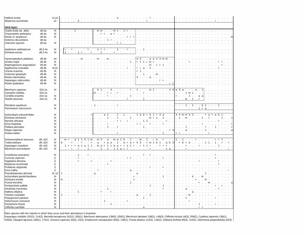
Halleria lucida s1,s2 . . . . . . . . . . . . . . . . . a . . . . . . . . . + . . . . . . . . . . . . . . . . . . . . . . . . .Maytenus acuminata s2 . . . . . 4 . . . . . . . . . . . . . . . . . . . . + . . . . . . . . . . . . . . . . . . . . r . . . . .
Herb layer:Oxalis livida var. altior d9.4a hl . . . . 1 . . . . . . m m . . . m 1 . 1 + . . . . . . . . . . . . . . . . . . . . . . . . . . . . . . . .Chasmanthe aethiopica d9.4a hl . . . . . . . . . . . . + + . a + . . . . . . . . . . . . . . . . . . . . . . . . . . . . . . . . . . . .Restio cf. perplexus d9.4a hl . . . . . . . . . . . . . . . . . . . . + r + . . . . . . . . . . . . . . . . . . . . . . . . . . . . . mDolichos decumbens d9.4a - . . . . . . . . . . . . . . 1 + . . . . . . . . . . . . . . . . . . . . . . . . . . . . . . . . . . . . .Unknown species d9.4a hl . . . . . . . . . . . . . . . . . + + . . . . . . . . . . . . . . . . . . . . . . . . . . . . . . . . . .
Asplenium aethiopicum d9.2-4a hl . + . + . . . . + . . 1 + + . . . 1 . . + . . . . 1 . . . . . . . . . . . . . . . . . . . . . . . . . . .Ehrharta erecta d9.2-4a hl . 1 . . . 1 + . . + . . 1 . . . + . . . . . . . . . . . . . . . . . . . . . . . . . . . . . . . . . . . .
Hymenophyllum peltatum d9.4b ml . . . . . . m . . . . m . . m . . . . . . . . a 4 . . a a 4 3 m m . . . . . . . . . . . . . . . . . . . .Aristea major d9.4b hl . . . . . . . . . . . . . . . . . . . . . 1 . + 1 1 r m + . . . . . . . . . . + . . . . . . . . + r . . .Elaphoglossum angustatum d9.4b hl . . . . . . . . . . . . . . . . . . . . . . . . . . . m . + + 1 . . . . . . . . . . . . . . . . . + . . .Agathosma crenulata d9.4b hl,s2 . . . . . . . . . . . . . . . . . . . . r . . r r a . 1 . . . . . . . . . . . . . . . . . . . . + . . . .Ursinia scariosa d9.4b hl . . . . . . . . . . . . . . . . . . . . . . . + 1 . . . . . . . . . . . . . . . . . . . . . . . . . . . .Unknown geophyte d9.4b hl . . . . . . . . . . . . . . . . . . . . . . . . . 1 . . . m . . . . . . . . . . . . . . . . . . . . . . .Restio intermedius d9.4b hl . . . . . . . . . . . . . . . . . . . . . . . 3 . . . a . . . . . . . . . . . . . . . . . . . . . . . . .Asparagus rubicundus d9.4b hl . . . . . . . . . . . . . . . . . . . . . . . . . . . . . . r + . . . . . . . . . . . . . . . . . . . . .Restio quadratus d9.4b hl . . . . . . . . . . . . . . . . . . . . . . . . . . . . . . . . . + 1 . . . . . . . . . . . . . . . . . .
Blechnum capense d10.1a hl . . . . . . . . . . . b 1 . . 4 . . . . . + . 1 . . . m 1 . . . . 4 4 a 5 a . . . a . 1 . . . . . . . . .Cassytha ciliolata d10.1a - . . . . . . . . . . m . . . r r . + . . . . . . . + . . . . . . . . . . . . 1 m 1 . . . . . . . . . . . .Centella eriantha d10.1a hl . . . . . . . . . . . . . . + . . . . . . 1 . . . . . . . . . . . . . r . . . 1 . . a a . . . . . . . . .Stoebe plumosa d10.1a hl . . . . . . . . . . . . . . . . . . . . + . . . . 1 . . . . . . . . . . . . m . 1 . + . . . . . . . . . .
Pteridium aquilinum hl . . . . . . . . . . 1 . . . . . . + . . . . . . . . . . . . . . . . . . . . 1 . 1 . . b 1 . . . 1 . . . .Pennisetum macrourum hl . . . . . . . . . . . . . . . . . . . . . . . . . . . . . . . . . . . . . . . . . . 1 + a . . . . . . . .
Ischyrolepis subverticillata hl . . . . . . . . . + . . . a 1 . . 1 . 1 . . . 1 a b + b 1 + 3 a . . . 3 4 m m 4 3 . . . + a + a b 1 . . .Ehrharta rehmannii hl . . . . . . . . . . . . . . 1 . . 1 . . . 1 . . . . . m + 1 . 1 . . . . 1 . m . . . . 1 . + . . . 1 . . 1Myrsine africana hl . . . . . . . . . . . . . . . . . + r . r . . . . 1 1 . . . . . + . . . . . . . . . . . . . . . + . . . .Erica hispidula hl . . . . . . . . . . . . . . r . . . . . . . . r + . . + . . . + . . . . . . . . . . . + . . . . . . . . +Pellaea pteroides hl . . . . . . . . . . . . . . 1 . . + . . . . . . . 1 . . . . . . . . . . . . 1 . . . . . + . . 1 . . . . +Elegia capensis hl . . . . . . . . . . . . . . . . . . . . . . . . . . . . . . . . . + 3 . . . a . . . . . 1 . . . . . . . aAristea bakeri hl . . . . . . . . . . . . . . . . . + . . . . . . . . . . . . . 1 . . . + + . . . . . . . . + . . . . . . .
Schoenoxiphium lanceum d9, d10 hl . m + . a 1 1 4 1 m . m 3 . a . m a 1 b . 1 . . m . 1 . r a . + . . . 1 . 1 . . . + . . . . . + + 1 . . .Todea barbara d9, d10 hl b . . + . . + . . + . a . + a a . 1 . a + a + 4 3 . + m 1 b 1 . a b 3 . + b + a . . . . 1 1 . 1 . + . + .Asparagus scandens d9, d10 hl . 1 + + + a 1 a 1 1 . m a + 1 1 b a + + 1 1 + . + 1 1 + . . + + + . . . . . + . . . r . . . . . 1 . . . .Blechnum punctulatum d9, d10 hl . . . + . + . . 1 . . . 1 . 1 . 1 1 a + r . . . . . . + . . . . 1 a . . . . + . . . . . . . . . . . . r .
Knowltonia vesicatoria hl . . . . . 1 . . r . . . . . . . . . . . . . . . . + . + . . . . . . . . . . . . . . . . . . . + . . . . .Cunonia capensis jl . . . . . + . . . . . . . . . . . . . . r + . . . . . . . . . + . . . . . . . . . . . . . . . + . . . . .Kiggelaria africana jl . . . . . + . . . + . . . . . + . . . . . . . . . . . . . . . . . . . . . . . . . . r . . . . . r . . . .Maytenus acuminata jl . . . . . . . . . . . . . . + . . . . . . . . . . . . . . . . . . . . . . . . . . . . . . . . . + . . . .Podalyria calyptrata jl . . . . . . . . . . . . . . . . . . . . . . . . . . . r . . . + . . . . . . . . . . . . . . . . . . . . .Erica caffra jl . . . . . . . . . . . + . . . . . . . . . a . . . . . . . . . . . . . . . . . . . . . . . . . . . . . r .Pseudobaeckea africana hl, s2 1 . . . . . . . . . a . . . . . . . . . . . . a . . . . . . . . . . . . . . . . . . . . 1 . . . . . . . .Ischyrolepis gaudichaudiana hl . . . . . . . . . . . . . . . . . . . . . . + . . . . . . . . 1 . . . . . . . . b . . m . . . . . . . . .Schizaea tenella hl m . . . . . . . . . . . . . . . . . . . . . 1 . . . . . . . . . . . . . . . . . . + . . m . . . . . . . .Ficinia brevifolia hl . . . . . . . . . . . . . . . . . . . . . 1 . . . . . . . . . . . . . . . . . . . . + . . m . . . . . . aPentaschistis pallida hl . . . . . . . . . . . . . . . . . . . . . . . . . . . 1 . . . 1 . . . . . . . . . . . . . . . + . + . . .Struthiola myrsinites hl . . . . . . . . . . . . . . 1 . . . . . . . . . . . . . . . . + . . . . . . a . . . . . . . . . + . . . .Halleria elliptica hl . . . . . 1 . . . . . . + . . r . . . . . . . . . . . . . . . . . . . . . . . . a . . . . . . . . . . . .Tetraria cuspidata hl 1 . . . . . . . . . . . . . . . . . . . . . . a . . . 1 . . . . . . . . . . . m . . . . . . . . . . . . .Pelargonium patulum hl . . . . . . . . . . . . . . . . . . . . . . . . . 1 . . . . . . . . . . . . 1 . . . . . . . . r . . . . .Helichrysum cymosum hl . . . . . . . . . . . . . 1 . . . . . . + . . . . . . . . . . . . . . . . . . + . . . . . . . . . . . . .Pentameris thuarii hl . . . . . . . . . . . . . . . 1 . . . . . . . . . . . . . . . . . . . . . . . . . . 1 . . . . r . . . . .Cliffortia ruscifolia hl . . . . . . . . . . . . . . . . . . . . . . . . . a . . . . . . . . . . . . . . . . r + . . . . . . . . .
Rare species with the relevés in which they occur and their abundance in brackets:Asparagus volubilis 102(2), 114(2), Berzelia lanuginosa 162(1), 265(1), Blechnum attenuatum 138(5), 200(2), Blechnum tabulare 138(2), 149(3), Cliffortia hirsuta 18(3), 209(2), Cyathea capensis 138(1), 194(5), Dipogon lignosus 169(1), 170(1), Drosera capensis 20(3), 22(2), Empleurum unicapsulare 90(5), 148(1), Ficinia distans 112(4), 116(2), Gibbaria ilicifolia 90(3), 110(2), Gleichenia polypodioides 62(3)
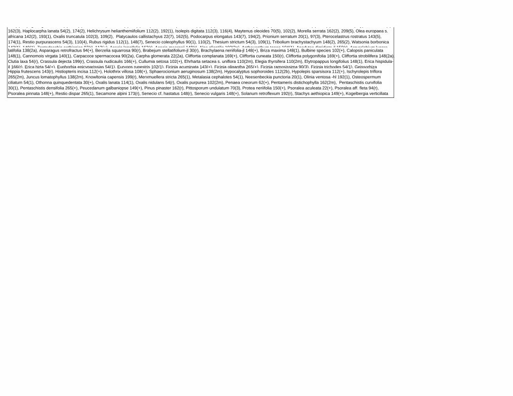
latifolia 138(2a), Asparagus retrofractus 94(+), Berzelia squarrosa 90(r), Brabejum stellatifolium-jl 30(r), Brachylaena neriifolia-jl 148(+), Briza maxima 148(1), Bulbine species 102(+), Calopsis paniculata 148(1), Cannomois virgata 140(1), Carpacoce spermacocea 90(2a), Carpha glomerata 22(2a), Cliffortia complanata 169(+), Cliffortia cuneata 150(r), Cliffortia polygonifolia 169(+), Cliffortia strobilifera 148(2a), Clutia laxa 54(r), Crassula dejecta 199(r), Crassula nudicaulis 166(+), Cullumia setosa 102(+), Ehrharta setacea s. uniflora 110(2m), Elegia thyrsifera 110(2m), Elytropappus longifolius 148(1), Erica hispidula-jl 166(r), Erica hirta 54(+), Euphorbia epicyparissias 54(1), Euryops rupestris 102(1), Ficinia acuminata 143(+), Ficinia oligantha 265(+), Ficinia ramosissima 90(3), Ficinia trichodes 54(1), Geissorhiza Hippia frutescens 143(r), Histiopteris incisa 112(+), Holothrix villosa 108(+), Sphaerocionium aeruginosum 138(2m), Hypocalyptus sophoroides 112(2b), Hypolepis sparsisora 112(+), Ischyrolepis triflora 265(2m), Juncus lomatophyllus 138(2m), Knowltonia capensis 199(r), Merxmuellera stricta 265(1), Metalasia cephalotes 54(1), Neesenbeckia punctoria 20(1), Olinia ventosa -hl 192(1), Osteospermum ciliatum 54(1), Othonna quinquedentata 30(+), Oxalis lanata 114(1), Oxalis nidulans 54(r), Oxalis purpurea 102(2m), Penaea cneorum 62(+), Pentameris distichophylla 162(2m), Pentaschistis curvifolia 30(1), Pentaschistis densifolia 265(+), Peucedanum galbaniopse 149(+), Pinus pinaster 162(r), Pittosporum undulatum 70(3), Protea neriifolia 150(+), Psoralea aculeata 22(+), Psoralea aff. fleta 94(r), Psoralea pinnata 148(+), Restio dispar 265(1), Secamone alpini 173(r), Senecio cf. hastatus 148(r), Senecio vulgaris 148(+), Solanum retroflexum 192(r), Stachys aethiopica 149(+), Kogelbergia verticillata 62( ) St b i 209( ) St b l 265( ) Th i i t 162(1) T h d t b l i 143( ) U i i kl i 90( ) U i i l 148( )
( ) p g g ( ) ( ) p ( ) ( ) p p ( ) ( ) ( ) ( ) ( ) ( ) p yp ( )162(3), Haplocarpha lanata 54(2), 174(2), Helichrysum helianthemiifolium 112(2), 192(1), Isolepis digitata 112(3), 116(4), Maytenus oleoides 70(5), 102(2), Morella serrata 162(2), 209(5), Olea europaea s. africana 142(2), 193(1), Oxalis truncatula 102(3), 109(2), Platycaulos callistachyus 22(7), 162(5), Podocarpus elongatus 143(7), 194(2), Prionium serratum 20(1), 97(3), Pterocelastrus rostratus 143(5), 174(1), Restio purpurascens 54(3), 110(4), Rubus rigidus 112(1), 148(7), Senecio coleophyllus 90(1), 110(2), Thesium strictum 54(3), 109(1), Tribolium brachystachyum 148(2), 265(2), Watsonia borbonica 143(1) 149(1) Zantedeschia aethiopica 97(r) 112(+) Acacia longifolia 162(r) Acacia mearnsii 148(r) Aloe plicatilis 102(2a) Anthoxanthum tongo 104(1) Apodytes dimidiata jl 150(r) Argyrolobium lunare
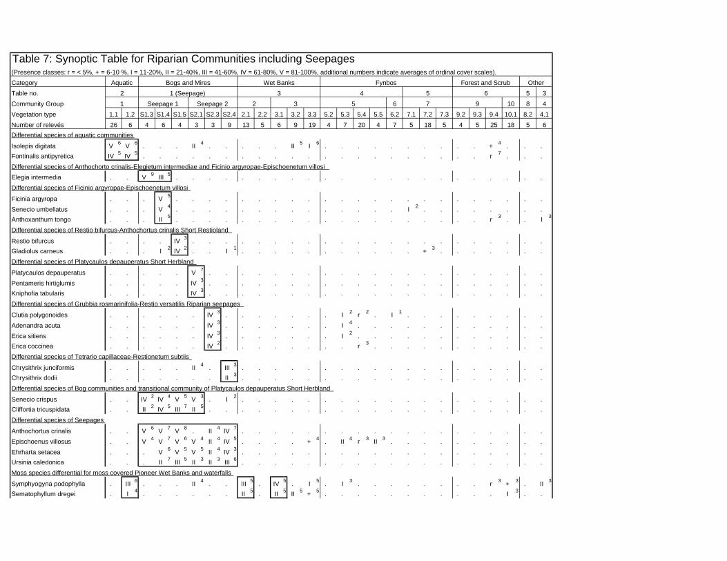
CategoryTable no.Community GroupVegetation typeNumber of relevés
Isolepis digitata V 6 V 6 . . . II 4 . . . . . II 5 I 6 . . . . . . . . . . + 4 . . .Fontinalis antipyretica IV 5 IV 5 . . . . . . . . . . . . . . . . . . . . . r 7 . . .Differential species of Anthochorto crinalis-Elegietum intermediae and Ficinio argyropae-Epischoenetum villosiElegia intermedia . . V 9 III 5 . . . . . . . . . . . . . . . . . . . . . .
Ficinia argyropa . . . V 5 . . . . . . . . . . . . . . . . . . . . . . .Senecio umbellatus . . . V 4 . . . . . . . . . . . . . . I 2 . . . . . . . .Anthoxanthum tongo . . . II 5 . . . . . . . . . . . . . . . . . . . r 3 . . I 3
Restio bifurcus . . . . IV 3 . . . . . . . . . . . . . . . . . . . . . .Gladiolus carneus . . . I 2 IV 2 . . I 1 . . . . . . . . . . . + 3 . . . . . . .
Platycaulos depauperatus . . . . . V 7 . . . . . . . . . . . . . . . . . . . . .Pentameris hirtiglumis . . . . . IV 3 . . . . . . . . . . . . . . . . . . . . .Kniphofia tabularis . . . . . IV 3 . . . . . . . . . . . . . . . . . . . . .
Clutia polygonoides . . . . . . IV 3 . . . . . . . I 2 r 2 . I 1 . . . . . . . . .Adenandra acuta . . . . . . IV 3 . . . . . . . I 4 . . . . . . . . . . . .Erica sitiens . . . . . . IV 3 . . . . . . . I 2 . . . . . . . . . . . .Erica coccinea . . . . . . IV 2 . . . . . . . . r 3 . . . . . . . . . . .
Chrysithrix junciformis . . . . . II 4 . III 3 . . . . . . . . . . . . . . . . . . .Chrysithrix dodii . . . . . . . II 3 . . . . . . . . . . . . . . . . . . .
Senecio crispus . . IV 2 IV 4 V 5 V 3 . I 2 . . . . . . . . . . . . . . . . . . .Cliffortia tricuspidata . . II 2 IV 5 III 7 II 5 . . . . . . . . . . . . . . . . . . . . .
Anthochortus crinalis . . V 6 V 7 V 8 . II 4 IV 7 . . . . . . . . . . . . . . . . . . .Epischoenus villosus . . V 4 V 7 V 6 V 4 II 4 IV 5 . . . . + 4 . II 4 r 3 II 3 . . . . . . . . . .Ehrharta setacea . . . V 6 V 5 V 5 II 4 IV 3 . . . . . . . . . . . . . . . . . . .Ursinia caledonica . . . II 7 III 5 II 3 II 3 III 6 . . . . . . . . . . . . . . . . . . .
Symphyogyna podophylla . III 6 . . . II 4 . . III 5 . IV 5 . I 5 . I 3 . . . . . . . . r 3 + 3 . II 3
Sematophyllum dregei . I 4 . . . . . . II 5 . II 5 II 5 + 5 . . . . . . . . . . . I 3 . .
(Presence classes: r = < 5%, + = 6-10 %, I = 11-20%, II = 21-40%, III = 41-60%, IV = 61-80%, V = 81-100%, additional numbers indicate averages of ordinal cover scales).
Table 7: Synoptic Table for Riparian Communities including Seepages
2 1 (Seepage) 3 4 5 6 5 3
25 18 5 618 5 4 520 4 7 59 19 4 79 13 5 66 4 3 39.4 10.1 8.2 4.17.2 7.3 9.2 9.35.4 5.5 6.2 7.13.2 3.3 5.2 5.3S2.4 2.1 2.2 3.1S1.4 S1.5 S2.1 S2.31.1 1.2 S1.3
26 6 4
9 10 8 43 5 6 71 Seepage 1 Seepage 2 2
Forest and ScrubFynbos OtherAquatic Bogs and Mires Wet Banks
Moss species differential for moss covered Pioneer Wet Banks and waterfalls
Differential species of aquatic communities
Differential species of Ficinio argyropae-Epischoenetum villosi
Differential species of Restio bifurcus-Anthochortus crinalis Short Restioland
Differential species of Platycaulos depauperatus Short Herbland
Differential species of Grubbia rosmarinifolia-Restio versatilis Riparian seepages
Differential species of Tetrario capillaceae-Restionetum subtiis
Differential species of Bog communities and transitional community of Platycaulos depauperatus Short Herbland
Differential species of Seepages
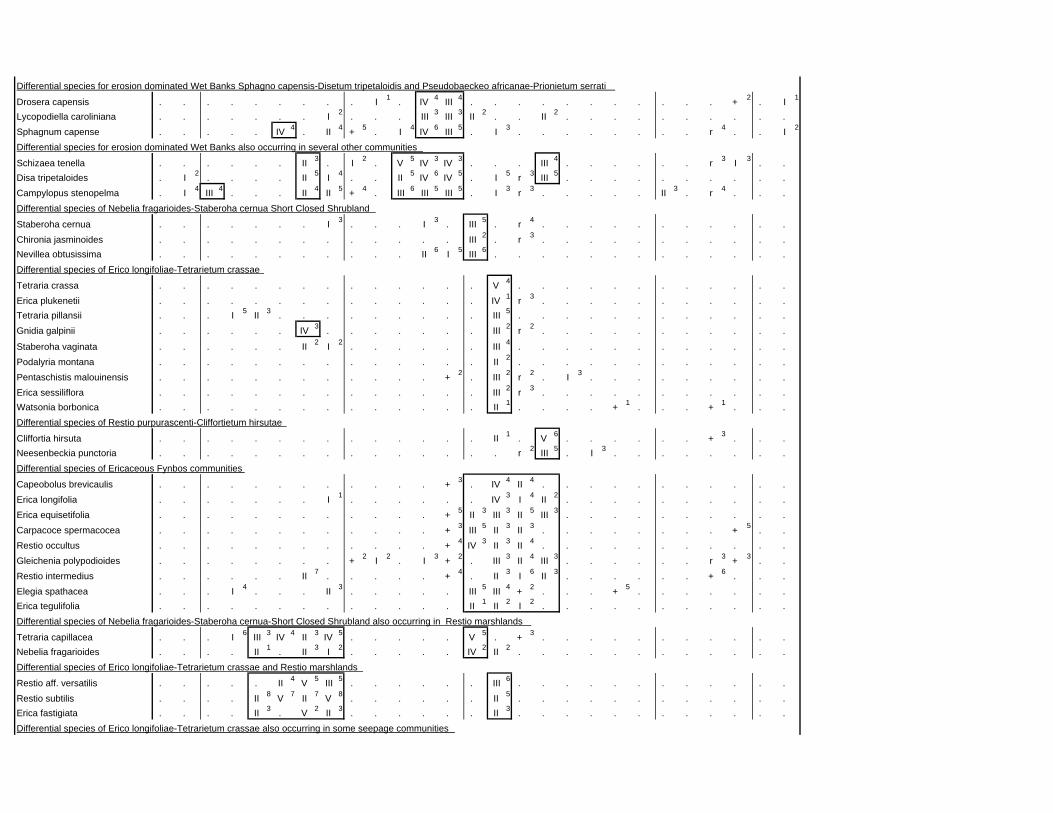
Drosera capensis . . . . . . . . . I 1 . IV 4 III 4 . . . . . . . . . . . + 2 . I 1
Lycopodiella caroliniana . . . . . . . I 2 . . . III 3 III 3 II 2 . . II 2 . . . . . . . . . .Sphagnum capense . . . . . IV 4 . II 4 + 5 . I 4 IV 6 III 5 . I 3 . . . . . . . . r 4 . . I 2
Schizaea tenella . . . . . . II 3 . I 2 . V 5 IV 3 IV 3 . . . III 4 . . . . . . r 3 I 3 . .Disa tripetaloides . I 2 . . . . II 5 I 4 . . II 5 IV 6 IV 5 . I 5 r 3 III 5 . . . . . . . . . .Campylopus stenopelma . I 4 III 4 . . . II 4 II 5 + 4 . III 6 III 5 III 5 . I 3 r 3 . . . . . II 3 . r 4 . . .
Staberoha cernua . . . . . . . I 3 . . . I 3 . III 5 . r 4 . . . . . . . . . . .Chironia jasminoides . . . . . . . . . . . . . III 2 . r 3 . . . . . . . . . . .Nevillea obtusissima . . . . . . . . . . . II 6 I 5 III 6 . . . . . . . . . . . . .
Tetraria crassa . . . . . . . . . . . . . . V 4 . . . . . . . . . . . .Erica plukenetii . . . . . . . . . . . . . . IV 1 r 3 . . . . . . . . . . .Tetraria pillansii . . . I 5 II 3 . . . . . . . . . III 5 . . . . . . . . . . . .Gnidia galpinii . . . . . . IV 3 . . . . . . . III 2 r 2 . . . . . . . . . . .
Staberoha vaginata . . . . . . II 2 I 2 . . . . . . III 4 . . . . . . . . . . . .Podalyria montana . . . . . . . . . . . . . . II 2 . . . . . . . . . . . .Pentaschistis malouinensis . . . . . . . . . . . . + 2 . III 2 r 2 . I 3 . . . . . . . . .Erica sessiliflora . . . . . . . . . . . . . . III 2 r 3 . . . . . . . . . . .Watsonia borbonica . . . . . . . . . . . . . . II 1 . . . . + 1 . . . + 1 . . .
Cliffortia hirsuta . . . . . . . . . . . . . . II 1 . V 6 . . . . . . + 3 . . .Neesenbeckia punctoria . . . . . . . . . . . . . . . r 2 III 5 . I 3 . . . . . . . .
Capeobolus brevicaulis . . . . . . . . . . . . + 3 . IV 4 II 4 . . . . . . . . . . .Erica longifolia . . . . . . . I 1 . . . . . . IV 3 I 4 II 2 . . . . . . . . . .Erica equisetifolia . . . . . . . . . . . . + 5 II 3 III 3 II 5 III 3 . . . . . . . . . .Carpacoce spermacocea . . . . . . . . . . . . + 3 III 5 II 3 II 3 . . . . . . . . + 5 . .Restio occultus . . . . . . . . . . . . + 4 IV 3 II 3 II 4 . . . . . . . . . . .Gleichenia polypodioides . . . . . . . . + 2 I 2 . I 3 + 2 . III 3 II 4 III 3 . . . . . . r 3 + 3 . .Restio intermedius . . . . . . II 7 . . . . . + 4 . II 3 I 6 II 3 . . . . . . + 6 . . .Elegia spathacea . . . I 4 . . . II 3 . . . . . III 5 III 4 + 2 . . . + 5 . . . . . . .Erica tegulifolia . . . . . . . . . . . . . II 1 II 2 I 2 . . . . . . . . . . .
Tetraria capillacea . . . I 6 III 3 IV 4 II 3 IV 5 . . . . . V 5 . + 3 . . . . . . . . . . .Nebelia fragarioides . . . . II 1 . II 3 I 2 . . . . . IV 2 II 2 . . . . . . . . . . . .
Restio aff. versatilis . . . . . II 4 V 5 III 5 . . . . . . III 6 . . . . . . . . . . . .Restio subtilis . . . . II 8 V 7 II 7 V 8 . . . . . . II 5 . . . . . . . . . . . .Erica fastigiata . . . . II 3 . V 2 II 3 . . . . . . II 3 . . . . . . . . . . . .
Differential species of Ericaceous Fynbos communities
Differential species of Nebelia fragarioides-Staberoha cernua-Short Closed Shrubland also occurring in Restio marshlands
Differential species of Erico longifoliae-Tetrarietum crassae and Restio marshlands
Differential species of Erico longifoliae-Tetrarietum crassae also occurring in some seepage communities
Differential species of Nebelia fragarioides-Staberoha cernua Short Closed Shrubland
Differential species of Erico longifoliae-Tetrarietum crassae
Differential species of Restio purpurascenti-Cliffortietum hirsutae
Differential species for erosion dominated Wet Banks Sphagno capensis-Disetum tripetaloidis and Pseudobaeckeo africanae-Prionietum serrati
Differential species for erosion dominated Wet Banks also occurring in several other communities
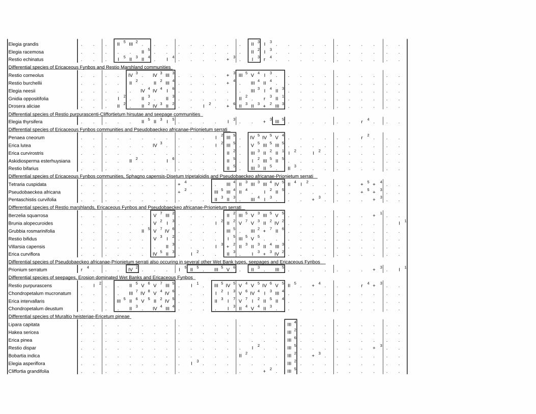
Elegia grandis . . . II 5 III 2 . . . . . . . . . II 3 I 3 . . . . . . . . . . .Elegia racemosa . . . . . II 5 . . . . . . . . II 2 I 3 . . . . . . . . . . .Restio echinatus . . . I 5 II 3 II 4 . I 4 . . . . + 3 . I 3 r 4 . . . . . . . . . . .
Restio corneolus . . . . IV 3 . IV 3 III 3 . . . . + 3 III 5 V 4 I 3 . . . . . . . . . . .Restio burchellii . . . . II 2 . II 2 III 4 . . . . + 4 . III 4 II 4 . . . . . . . . . . .Elegia neesii . . . . . IV 4 IV 4 I 6 . . . . . . III 3 I 4 II 3 . . . . . . . . . .Gnidia oppositifolia . . . I 2 . II 3 . II 3 . . . . . II 2 . r 3 II 1 . . . . . . . . . .Drosera aliciae . . . II 2 . II 2 IV 3 II 2 . . I 2 . + 6 II 3 II 3 + 2 III 3 . . . . . . . . . .
Elegia thyrsifera . . . . . II 5 II 3 I 5 . . . . I 3 . . + 3 III 5 . . . . . . r 4 . . .
Penaea cneorum . . . . . . . . . . . I 2 III 5 . IV 5 IV 5 V 4 . . . . . . r 2 . . .Erica lutea . . . . . . IV 3 . . . . I 2 III 5 . V 5 III 5 III 5 . . . . . . . . . .Erica curvirostris . . . . . . . . . . . . II 2 . III 3 II 2 II 1 I 2 . I 2 . . . . . . .Askidiosperma esterhuysiana . . . . II 2 . . I 6 . . . . II 5 . I 2 III 5 II 5 . . . . . . . . . .Restio bifarius . . . . . . . . . . . . II 5 . III 3 II 5 . II 3 . . . . . . . . .
Tetraria cuspidata . . . . . . . . + 4 . . . III 4 II 3 III 3 III 4 IV 5 II 4 I 2 . . . . + 5 + 4 . .Pseudobaeckea africana . . . . . . . . + 2 . . III 5 III 4 II 4 . I 2 II 5 . . . . . . + 5 + 3 . .Pentaschistis curvifolia . . . . . . . . . . . II 3 II 3 . III 4 I 3 . . . + 3 . . . . + 3 . .
Berzelia squarrosa . . . . . . V 7 III 2 . . . . II 2 III 5 V 3 III 5 V 5 . . . . . . . + 1 . .Brunia alopecuroides . . . . . . V 2 I 3 . . . I 2 II 2 V 7 V 3 II 2 IV 2 . . . . . . . . . I 1
Grubbia rosmarinifolia . . . . . II 5 V 7 IV 6 . . . . III 5 . III 2 + 7 II 6 . . . . . . . . . .Restio bifidus . . . . . . V 3 I 2 . . . . I 5 III 5 V 5 . . . . . . . . . . . .Villarsia capensis . . . . . . . II 3 . . . I 3 + 2 II 3 II 3 II 4 III 3 . . . . . . . . . .Erica curviflora . . . . . . IV 5 II 3 . I 2 . . II 3 . I 3 + 3 IV 2 . . . . . . . . . .
Prionium serratum r 4 . . . IV 2 . . . I 5 II 5 . III 5 V 6 . II 3 . III 5 . . . . . . . + 3 . I 1
Restio purpurascens . I 2 . . II 5 V 6 V 7 III 5 . I 1 . III 5 IV 5 V 4 V 5 IV 6 V 5 II 5 . + 4 . . . r 4 + 3 . .Chondropetalum mucronatum . . . . III 7 IV 8 V 4 IV 6 . . . I 2 I 3 V 6 IV 4 I 3 III 4 . . . . . . . . . .Erica intervallaris . . . III 5 II 6 V 5 II 2 IV 5 . . . II 3 I 7 V 7 I 2 II 5 II 4 . . . . . . . . . .Chondropetalum deustum . . . . II 3 . IV 4 III 4 . . . . I 3 II 4 V 4 II 3 . . . . . . . . . . .
Lipara capitata . . . . . . . . . . . . . . . . . III 4 . . . . . . . . .Hakea sericea . . . . . . . . . . . . . . . . . III 2 . . . . . . . . .Erica pinea . . . . . . . . . . . . . . . . . III 6 . . . . . . . . .Restio dispar . . . . . . . . . . . . . . I 2 . . III 5 . . . . . . + 3 . .Bobartia indica . . . . . . . . . . . . . II 2 . . . III 2 . + 3 . . . . . . .Elegia asperiflora . . . . . . . . . I 3 . . . . . . . III 2 . . . . . . . . .Cliffortia grandifolia . . . . . . . . . . . . . . . + 2 . III 5 . . . . . . . . .
Differential species of Restio marshlands, Ericaceous Fynbos and Pseudobaeckeo africanae-Prionietum serrati
Differential species of Pseudobaeckeo africanae-Prionietum serrati also occuring in several other Wet Bank types, seepages and Ericaceous Fynbos
Differential species of seepages, Erosion dominated Wet Banks and Ericaceous Fynbos
Differential species of Muraltio heisteriae-Ericetum pineae
Differential species of Ericaceous Fynbos and Restio Marshland communities
Differential species of Restio purpurascenti-Cliffortietum hirsutae and seepage communities
Differential species of Ericaceous Fynbos communities and Pseudobaeckeo africanae-Prionietum serrati
Differential species of Ericaceous Fynbos communities, Sphagno capensis-Disetum tripetaloidis and Pseudobaeckeo africanae-Prionietum serrati
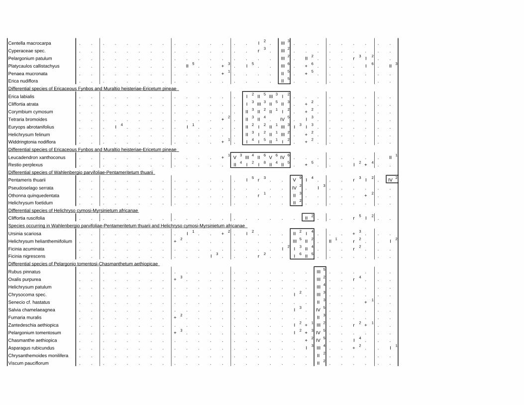
Centella macrocarpa . . . . . . . . . . . . . . . I 2 . III 3 . . . . . . . . .Cyperaceae spec. . . . . . . . . . . . . . . . r 3 . III 2 . . . . . . . . .Pelargonium patulum . . . . . . . . . . . . . . . . . III 2 . II 2 . . . r 3 I 2 . .Platycaulos callistachyus . . . . . . . . . II 5 . . + 3 . I 5 . . III 6 . + 6 . . . . I 6 . II 3
Penaea mucronata . . . . . . . . . . . . + 1 . . . . II 5 . + 5 . . . . . . .Erica nudiflora . . . . . . . . . . . . . . . . . II 5 . . . . . . . . .
Erica labialis . . . . . . . . . . . . . . I 2 II 5 III 3 I 2 . . . . . . . . .Cliffortia atrata . . . . . . . . . . . . . . I 3 III 3 II 5 II 3 . + 2 . . . . . . .Corymbium cymosum . . . . . . . . . . . . . . II 3 II 2 II 1 I 2 . + 2 . . . . . . .Tetraria bromoides . . . . . . . . . . . . + 2 . II 3 II 4 . IV 5 . I 3 . . . . . . .Euryops abrotanifolius . . . I 4 . . . . . I 1 . . . . II 2 I 2 II 1 III 3 I 3 I 3 . . . . . . .Helichrysum felinum . . . . . . . . . . . . . . II 3 I 2 II 1 III 2 . + 2 . . . . . . .Widdringtonia nodiflora . . . . . . . . . . . . + 1 . I 4 I 5 II 1 I 2 . + 2 . . . . . . .
Leucadendron xanthoconus . . . . . . . . . . . . + 1 V 3 III 4 II 6 V 6 IV 6 . . . . . . . . II 1
Restio perplexus . . . . . . . . . . . . . II 4 I 2 I 8 II 4 II 5 . + 5 . . . I 2 + 4 . .
Pentameris thuarii . . . . . . . . . . . . . . I 5 r 3 . . V 9 I 4 . . . r 3 I 2 . IV 2
Pseudoselago serrata . . . . . . . . . . . . . . . . . . IV 2 . I 3 . . . . . .Othonna quinquedentata . . . . . . . . . . . . . . . r 1 . . II 3 . . . . . + 2 . .Helichrysum foetidum . . . . . . . . . . . . . . . . . . II 2 . . . . . . . .
Cliffortia ruscifolia . . . . . . . . . . . . . . . . . . . II 2 . . . r 5 I 2 . .
Ursinia scariosa . . . . . . . . . I 1 . . + 2 . I 2 . . . II 2 I 4 . . . + 3 . . .Helichrysum helianthemiifolium . . . . . . . . + 2 . . . . . . . . . III 5 II 2 . II 1 . r 2 . . I 2
Ficinia acuminata . . . . . . . . . . . . . . . . . I 2 I 3 II 4 . . . r 2 . . .Ficinia nigrescens . . . . . . . . . . . I 3 . . . r 2 . . I 6 II 5 . . . . . . .
Rubus pinnatus . . . . . . . . . . . . . . . . . . . . III 5 . . . . . .Oxalis purpurea . . . . . . . . + 3 . . . . . . . . . . . III 2 . . r 4 . . .Helichrysum patulum . . . . . . . . . . . . . . . . . . . . III 4 . . . . . .Chrysocoma spec. . . . . . . . . . . . . . . . . . . I 2 . III 3 . . . . . .Senecio cf. hastatus . . . . . . . . . . . . . . . . . . . . II 3 . . . + 1 . .Salvia chamelaeagnea . . . . . . . . . . . . . . . . . . I 3 . IV 5 . . . . . .Fumaria muralis . . . . . . . . + 2 . . . . . . . . . . . II 3 . . . . . .Zantedeschia aethiopica . . . . . . . . . . . . . . . . . . I 2 + 1 III 2 . . r 2 + 1 . .Pelargonium tomentosum . . . . . . . . + 3 . . . . . . . . . I 2 + 3 IV 5 . . . . . .Chasmanthe aethiopica . . . . . . . . . . . . . . . . . . . + 2 IV 5 . . I 4 . . .Asparagus rubicundus . . . . . . . . . . . . . . . . . . . I 3 III 4 . . + 2 . . I 1
Chrysanthemoides monilifera . . . . . . . . . . . . . . . . . . . . II 2 . . . . . .Viscum pauciflorum . . . . . . . . . . . . . . . . . . . . II 2 . . . . . .
Species occurring in Wahlenbergio parvifoliae-Pentameritetum thuarii and Helichryso cymosi-Myrsinietum africanae
Differential species of Pelargonio tomentosi-Chasmanthetum aethiopicae
Differential species of Ericaceous Fynbos and Muraltio heisteriae-Ericetum pineae
Differential species of Ericaceous Fynbos and Muraltio heisteriae-Ericetum pineae
Differential species of Wahlenbergio parvifoliae-Pentameritetum thuarii
Differential species of Helichryso cymosi-Myrsinietum africanae
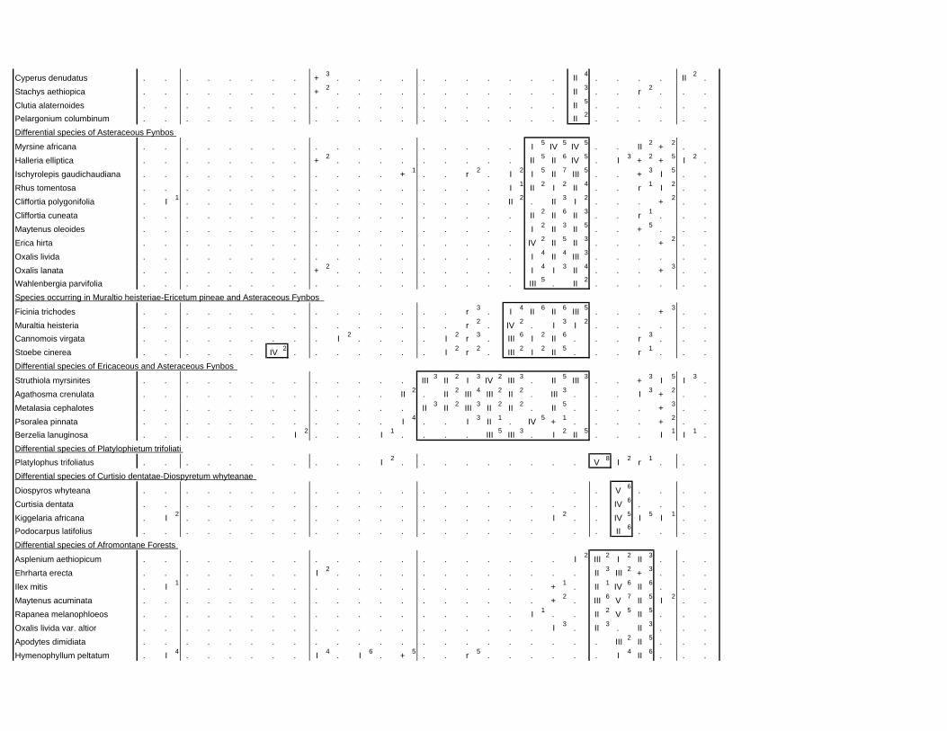
Cyperus denudatus . . . . . . . . + 3 . . . . . . . . . . . II 4 . . . . II 2 .Stachys aethiopica . . . . . . . . + 2 . . . . . . . . . . . II 3 . . r 2 . . .Clutia alaternoides . . . . . . . . . . . . . . . . . . . . II 5 . . . . . .Pelargonium columbinum . . . . . . . . . . . . . . . . . . . . II 2 . . . . . .
Myrsine africana . . . . . . . . . . . . . . . . . . I 5 IV 5 IV 5 . . II 2 + 2 . .Halleria elliptica . . . . . . . . + 2 . . . . . . . . . II 5 II 6 IV 5 . I 3 + 2 + 5 I 2 .Ischyrolepis gaudichaudiana . . . . . . . . . . . . + 1 . . r 2 . I 2 I 5 II 7 III 5 . . + 3 I 5 . .Rhus tomentosa . . . . . . . . . . . . . . . . . I 1 II 2 I 2 II 4 . . r 1 I 2 . .Cliffortia polygonifolia . I 1 . . . . . . . . . . . . . . . II 2 . II 3 I 2 . . . + 2 . .Cliffortia cuneata . . . . . . . . . . . . . . . . . . II 2 II 6 II 3 . . r 1 . . .Maytenus oleoides . . . . . . . . . . . . . . . . . . I 2 II 3 II 5 . . + 5 . . .Erica hirta . . . . . . . . . . . . . . . . . . IV 2 II 5 II 3 . . . + 2 . .Oxalis livida . . . . . . . . . . . . . . . . . . I 4 II 4 III 3 . . . . . .Oxalis lanata . . . . . . . . + 2 . . . . . . . . . I 4 I 3 II 4 . . . + 3 . .Wahlenbergia parvifolia . . . . . . . . . . . . . . . . . . III 5 . II 2 . . . . . .
Ficinia trichodes . . . . . . . . . . . . . . . r 3 . I 4 II 6 II 6 III 5 . . . + 3 . .Muraltia heisteria . . . . . . . . . . . . . . . r 2 . IV 2 . I 3 I 2 . . . . . .Cannomois virgata . . . . . . . . . I 2 . . . . I 2 r 3 . III 6 I 2 II 6 . . . r 3 . . .Stoebe cinerea . . . . . . IV 2 . . . . . . . I 2 r 2 . III 2 I 2 II 5 . . . r 1 . . .
Struthiola myrsinites . . . . . . . . . . . . . III 3 II 2 I 3 IV 2 III 3 . II 5 III 3 . . + 3 I 5 I 3 .Agathosma crenulata . . . . . . . . . . . . II 2 . II 2 III 4 III 2 II 2 . III 3 . . . I 3 + 2 . .Metalasia cephalotes . . . . . . . . . . . . . II 3 II 2 III 3 II 2 II 2 . II 5 . . . . + 3 . .Psoralea pinnata . . . . . . . . . . . . I 4 . . I 3 II 1 . IV 5 + 1 . . . . + 2 . .Berzelia lanuginosa . . . . . . . I 2 . . . I 1 . . . . III 5 III 3 . I 2 II 5 . . . I 1 I 1 .
Platylophus trifoliatus . . . . . . . . . . . I 2 . . . . . . . . . V 8 I 2 r 1 . . .
Diospyros whyteana . . . . . . . . . . . . . . . . . . . . . . V 6 . . . .Curtisia dentata . . . . . . . . . . . . . . . . . . . . . . IV 6 . . . .Kiggelaria africana . I 2 . . . . . . . . . . . . . . . . . I 2 . . IV 5 I 5 I 1 . .Podocarpus latifolius . . . . . . . . . . . . . . . . . . . . . . II 6 . . . .
Asplenium aethiopicum . . . . . . . . . . . . . . . . . . . . I 2 III 2 I 2 II 3 . . .Ehrharta erecta . . . . . . . . I 2 . . . . . . . . . . . . II 3 III 2 + 3 . . .Ilex mitis . I 1 . . . . . . . . . . . . . . . . . + 1 . II 1 IV 6 II 6 . . .Maytenus acuminata . . . . . . . . . . . . . . . . . . . + 2 . III 6 V 7 II 5 I 2 . .Rapanea melanophloeos . . . . . . . . . . . . . . . . . . I 1 . . II 2 V 5 II 5 . . .Oxalis livida var. altior . . . . . . . . . . . . . . . . . . . I 3 . II 3 . II 3 . . .Apodytes dimidiata . . . . . . . . . . . . . . . . . . . . . . III 2 II 5 . . .Hymenophyllum peltatum . I 4 . . . . . . I 4 . I 6 . + 5 . . r 5 . . . . . . I 4 II 6 . . .
Differential species of Ericaceous and Asteraceous Fynbos
Differential species of Platylophietum trifoliati
Differential species of Curtisio dentatae-Diospyretum whyteanae
Differential species of Afromontane Forests
Differential species of Asteraceous Fynbos
Species occurring in Muraltio heisteriae-Ericetum pineae and Asteraceous Fynbos
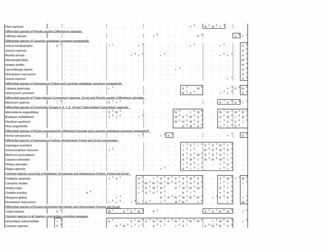
Olea capensis . . . . . . . . . . . . . . . . . . . + 5 . III 5 III 6 I 2 . . .
Cliffortia odorata . . . . . . . . . . . . . . I 3 . . . . . II 3 . . . . V 8 I 1
Juncus lomatophyllus . II 2 . . . . . . I 1 . . . + 2 . . . . . . + 2 . . . r 4 . . V 6
Juncus capensis . . . . . . . . . . . . . . . . . . . . . . . . . . V 3
Morella serrata . . . . . . . . . . . I 5 I 5 . . r 2 . . . . . . . r 5 + 2 . V 2
Wimmerella bifida . . . . . . . . . . . . . . . . . . . . . . . . . . IV 3
Isolepis prolifer . . . . . . . . . . . . . . . . . . . . . . . . . . IV 4
Laurembergia repens . . . . . . . . . . . . . . . . . I 2 . . . . . . . . II 3
Pennisetum macrourum . . . . . . . . . . . . . . . . . . . . . . . . . . II 2
Acacia mearnsii . . . . . . . . . . . . . . . . . . . . . . . . + 1 . II 2
Calopsis paniculata . . . . . . . . + 2 . . . . . . . . . II 3 . III 5 . . . + 3 II 3 IV 4
Helichrysum cymosum . . . . . . . . . . . . . . . . . . II 5 II 3 . . . + 3 + 2 . II 3
Blechnum capense . I 2 . . . . . . II 2 I 2 . . . . . . . . . . . . . II 7 II 6 II 6 I 1
Metrosideros angustifolius . . . . . . . . II 5 IV 5 . . . . . . . IV 6 . I 6 III 5 . . III 7 IV 7 III 4 IV 2
Brabejum stellatifolium . . . . . . . . I 5 I 2 . . I 2 . . . . III 5 II 2 III 6 II 5 . . II 6 III 6 I 8 III 2
Pteridium aquilinum . . . . . . . . . . . . . . . . . III 5 IV 6 III 5 V 7 . . + 3 II 5 V 6 I 2
Rhus angustifolia . . . . . . . . . . . . . . . . . . II 6 III 4 V 6 . . + 2 I 4 II 6 .
Ficinia ramosissima . . . . . . . . . . . . I 4 . . I 5 II 7 . . . . . . . + 7 . II 2
Asparagus scandens . . . . . . . . . . . . . . . . . . I 3 II 4 I 2 V 2 V 5 IV 4 I 2 . .Schoenoxiphium lanceum . . . . . . . . I 3 . . . . . . . . . I 2 I 3 . IV 5 V 6 III 5 II 3 . .Blechnum punctulatum . . . . . . . . . . . . . . . . . . II 3 II 4 III 3 II 2 II 3 II 4 I 2 . .Cassine schinoides . . . . . . . . . . . . . . . . . . II 2 III 5 I 2 III 5 IV 5 III 6 I 4 . .Pellaea pteroides . . . . . . . . . . . . . . . . . . I 4 II 6 I 3 . . I 3 II 3 . .Elegia capensis . . . . . . . . . . . . . . . r 3 . . II 6 I 3 I 5 . . + 6 I 5 . .
Podalyria calyptrata . . . . . . . . I 2 II 1 . . II 5 . I 2 II 5 II 2 V 4 II 5 III 6 II 5 . . II 5 III 6 I 1 III 3
Cassytha ciliolata . . . . . . . . . . . . II 3 IV 3 IV 3 IV 3 IV 4 V 4 II 2 II 3 II 5 . . I 2 I 3 . I 1
Aristea major . . . . . . . . . . . . I 2 II 2 III 2 III 2 . V 2 III 2 IV 4 III 2 . . II 3 I 2 . .Centella eriantha . . . . . II 3 . . . . . . + 3 II 2 II 2 II 5 . . II 2 I 5 . . . + 3 II 5 . .Diospyros glabra . . . . . . . . . I 1 . . . . . II 2 II 2 IV 2 III 2 IV 4 IV 2 . I 2 II 3 II 3 . I 1
Pennisetum macrourum . . . . . . . . + 5 I 3 . I 4 + 1 II 4 . I 5 . III 4 IV 4 . I 4 . . . I 4 . III 7
Todea barbara . II 5 . . . . . . III 2 . II 3 II 2 III 2 . II 2 . . . . . . II 2 II 2 IV 6 III 5 . I 2
Ischyrolepis subverticillata . I 2 . . . . . . II 3 . . II 2 III 5 II 4 III 5 IV 6 II 4 IV 6 II 3 IV 6 III 5 . I 2 III 5 IV 6 . I 2
Cunonia capensis . II 2 . . . . . . . II 2 III 3 I 1 I 1 . II 2 r 1 . I 2 II 1 . . II 5 IV 5 IV 7 II 5 . .
Differential species of Erosion-dominated Wet Banks and Afromontane Forests and Scrub
Common species to all riparian communities excluding seepages
Differential species of Community Groups 4, 6, 7, 8, 10 and Todeo barbari-Cunonietum capensis
Differential species of Restio purpurascenti-Cliffortietum hirsutae and Laurentio arabideae-Juncetum lomatophylli
Differential species of Asteraceous Fynbos, Afromontane Forest and Scrub communities
Common species occurring in Wetbanks, Ericaceous and Asteraceous Fynbos, Forest and Scrub
Differential species of Pteridio aquilini-Cliffortietum odoratae
Differential species of Laurentio arabideae-Juncetum lomatophylli
Differential species of Asteraceous Fynbos and Laurentio arabideae-Juncetum lomatophylli
Differential species of Todeo barbari-Cunonietum capensis, Scrub and Pteridio aquilini-Cliffortietum odoratae
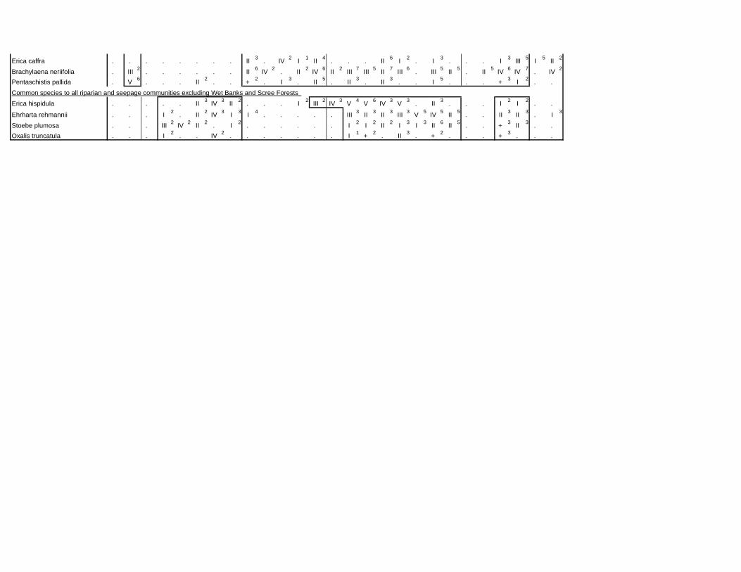
Erica caffra . . . . . . . . II 3 . IV 2 I 1 II 4 . . . II 6 I 2 . I 3 . . . I 3 III 5 I 5 II 2
Brachylaena neriifolia . III 2 . . . . . . II 6 IV 2 . II 2 IV 6 II 2 III 7 III 5 II 7 III 6 . III 5 II 5 . II 5 IV 6 IV 7 . IV 2
Pentaschistis pallida . V 6 . . . II 2 . . + 2 . I 3 . II 5 . II 3 . II 3 . . I 5 . . . + 3 I 2 . .
Erica hispidula . . . . . II 3 IV 3 II 2 . . . I 2 III 2 IV 3 V 4 V 6 IV 3 V 3 . II 3 . . . I 2 I 2 . .
Ehrharta rehmannii . . . I 2 . II 2 IV 3 I 3 I 4 . . . . . III 3 II 3 II 3 III 3 V 5 IV 5 II 5 . . II 3 II 3 . I 3
Stoebe plumosa . . . III 2 IV 2 II 2 . I 2 . . . . . . I 2 I 2 II 2 I 3 I 3 II 6 II 5 . . + 3 II 3 . .Oxalis truncatula . . . I 2 . . IV 2 . . . . . . . I 1 + 2 . II 3 . + 2 . . . + 3 . . .
Common species to all riparian and seepage communities excluding Wet Banks and Scree Forests
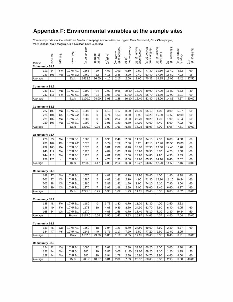
Appendix F: Environmental variables at the sample sitesCommunity codes indicated with an S refer to seepage communities; soil types: Fw = Fernwood, Ch = Champagne,Ms = Mispah, Ma = Magwa, Oa = Oakleaf, Gs = Glenrosa
Releve
Transect
Soil type
Soil colour
Altitude (in m
)
Slope (in
degrees)
pH (H
2 O)
Resistance (in
kilo-Ohm
s)
Gravel fraction
(in %)
Coarse sand
fraction (in %)
Medium
sand fraction (in %
)
Fine sand fraction (in %
)
Silt fraction (in
%)
Organic
matter (in %
)
Soil depth (in
cm)
Community S1.1111 34 Fw 10YR 4/1 1365 20 4.09 1.91 0.10 0.80 77.30 10.50 11.40 3.82 60233 106 Ma 10YR 3/2 1460 32 4.11 2.35 3.90 2.40 63.40 17.80 16.50 7.02 15
Average Dark 1412.5 26.00 4.10 2.13 2.00 1.60 70.35 14.15 13.95 5.42 37.50
Community S1.2241 110 Ma 10YR 3/1 1100 24 3.90 0.65 20.30 15.90 49.90 17.30 16.80 6.53 40242 111 Fw 10YR 4/1 1100 24 3.96 1.91 11.90 16.90 55.70 14.50 12.90 2.81 60
Average Dark 1100.0 24.00 3.93 1.28 16.10 16.40 52.80 15.90 14.85 4.67 50.00
Community S1.3227 100 Ma 10YR 3/1 1200 0 4.13 1.17 8.30 27.90 65.10 4.00 3.00 5.97 60228 101 Ch 10YR 2/2 1200 0 3.74 1.53 8.60 6.90 64.20 15.50 13.50 12.09 60229 102 Ma 10YR 3/1 1200 0 3.90 2.52 3.50 23.20 70.20 4.70 1.90 5.34 60230 103 Ma 10YR 3/1 1200 0 3.91 1.21 6.30 14.10 72.60 7.40 5.90 7.02 60
Average Dark 1200.0 0.00 3.92 1.61 6.68 18.03 68.03 7.90 6.08 7.61 60.00
Community S1.4226 99 Ma 10YR 3/1 1200 0 3.90 2.46 2.50 11.90 74.10 7.10 6.80 4.68 60231 104 Ch 10YR 2/2 1370 0 3.74 1.52 2.60 0.20 47.10 22.20 30.50 19.89 60232 105 Oa 10YR 3/1 1370 0 3.81 2.06 0.40 13.90 57.90 13.90 14.40 2.40 60243 112 Ma 10YR 3/1 1125 0 4.04 1.83 3.70 10.20 76.90 8.70 4.20 5.58 60244 113 Ma 10YR 3/1 1125 0 4.01 2.87 2.60 13.20 74.80 7.20 4.90 3.39 60259 125 - 10YR 3/1 - 7 4.78 1.95 8.50 12.20 65.30 14.10 8.40 7.02 60
Average Dark 1238.0 1.17 4.05 2.12 3.38 10.27 66.02 12.20 11.53 7.16 60.00
Community S1.5188 77 Ma 10YR 3/1 1070 6 4.08 1.37 0.70 23.80 70.40 4.00 1.80 4.88 60201 87 Ch 10YR 3/1 1280 7 4.02 1.61 2.10 4.90 71.30 12.70 11.10 10.34 60202 88 Ch 10YR 3/1 1280 7 3.85 1.82 1.50 8.90 74.10 9.10 7.90 8.00 60203 89 Ch 10YR 3/1 1270 7 3.96 1.96 2.60 7.00 78.00 8.40 6.60 8.87 60
Average Dark 1225.0 6.75 3.98 1.69 1.73 11.15 73.45 8.55 6.85 8.02 60.00
Community S2.1135 48 Fw 10YR 5/1 1180 0 3.73 1.82 0.70 11.20 81.30 4.00 3.50 2.63 -136 49 Fw 10YR 3/3 1175 10 4.05 0.89 8.60 24.30 62.70 6.60 6.40 9.95 60165 64 Ch 10YR 3/1 1170 - 4.08 1.58 0.70 15.40 78.10 3.10 3.30 10.34 50
Average Brown 1175.0 5.00 3.95 1.43 3.33 16.97 74.03 4.57 4.40 7.64 55.00
Community S2.2131 46 Oa 10YR 4/1 1160 18 3.94 1.21 5.80 24.50 69.60 3.60 2.30 5.77 60134 47 Ms 10YR 4/1 1145 40 3.76 1.17 7.90 9.80 77.20 2.50 10.50 2.05 -
Average Grey 1152.5 29.00 3.85 1.19 6.85 17.15 73.40 3.05 6.40 3.91 60.00
Community S2.3124 42 Oa 10YR 3/1 1000 12 3.63 1.16 7.90 33.80 60.20 3.00 3.00 3.90 40127 44 Ms 10YR 5/1 980 10 3.86 3.05 11.60 27.60 69.20 2.10 1.20 1.35 20128 44 Ma 10YR 3/1 980 10 3.94 1.78 2.50 16.80 74.70 3.90 4.60 4.00 60
Average Dark 986.7 10.67 3.81 2.00 7.33 26.07 68.03 3.00 2.93 3.08 40.00
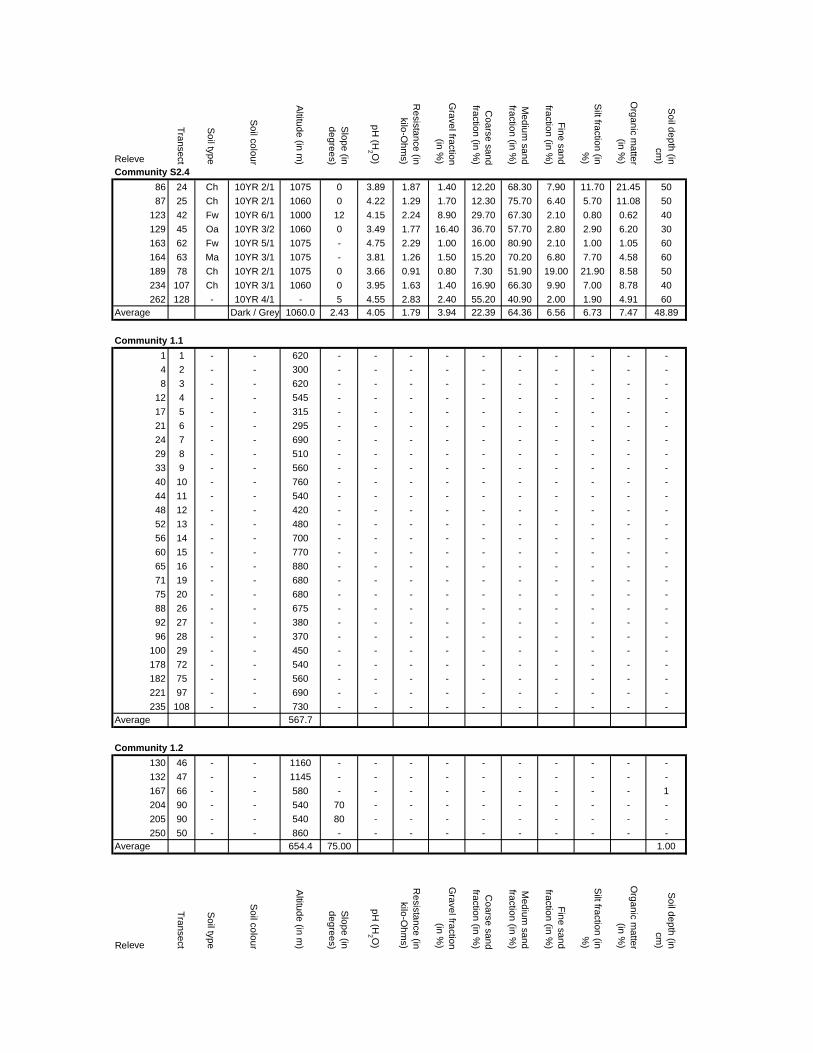
Releve
Transect
Soil type
Soil colour
Altitude (in m
)
Slope (in
degrees)
pH (H
2 O)
Resistance (in
kilo-Ohm
s)
Gravel fraction
(in %)
Coarse sand
fraction (in %)
Medium
sand fraction (in %
)
Fine sand fraction (in %
)
Silt fraction (in
%)
Organic m
atter (in %
)
Soil depth (in
cm)
Community S2.486 24 Ch 10YR 2/1 1075 0 3.89 1.87 1.40 12.20 68.30 7.90 11.70 21.45 5087 25 Ch 10YR 2/1 1060 0 4.22 1.29 1.70 12.30 75.70 6.40 5.70 11.08 50
123 42 Fw 10YR 6/1 1000 12 4.15 2.24 8.90 29.70 67.30 2.10 0.80 0.62 40129 45 Oa 10YR 3/2 1060 0 3.49 1.77 16.40 36.70 57.70 2.80 2.90 6.20 30163 62 Fw 10YR 5/1 1075 - 4.75 2.29 1.00 16.00 80.90 2.10 1.00 1.05 60164 63 Ma 10YR 3/1 1075 - 3.81 1.26 1.50 15.20 70.20 6.80 7.70 4.58 60189 78 Ch 10YR 2/1 1075 0 3.66 0.91 0.80 7.30 51.90 19.00 21.90 8.58 50234 107 Ch 10YR 3/1 1060 0 3.95 1.63 1.40 16.90 66.30 9.90 7.00 8.78 40262 128 - 10YR 4/1 - 5 4.55 2.83 2.40 55.20 40.90 2.00 1.90 4.91 60
Average Dark / Grey 1060.0 2.43 4.05 1.79 3.94 22.39 64.36 6.56 6.73 7.47 48.89
Community 1.11 1 - - 620 - - - - - - - - - -4 2 - - 300 - - - - - - - - - -8 3 - - 620 - - - - - - - - - -
12 4 - - 545 - - - - - - - - - -17 5 - - 315 - - - - - - - - - -21 6 - - 295 - - - - - - - - - -24 7 - - 690 - - - - - - - - - -29 8 - - 510 - - - - - - - - - -33 9 - - 560 - - - - - - - - - -40 10 - - 760 - - - - - - - - - -44 11 - - 540 - - - - - - - - - -48 12 - - 420 - - - - - - - - - -52 13 - - 480 - - - - - - - - - -56 14 - - 700 - - - - - - - - - -60 15 - - 770 - - - - - - - - - -65 16 - - 880 - - - - - - - - - -71 19 - - 680 - - - - - - - - - -75 20 - - 680 - - - - - - - - - -88 26 - - 675 - - - - - - - - - -92 27 - - 380 - - - - - - - - - -96 28 - - 370 - - - - - - - - - -
100 29 - - 450 - - - - - - - - - -178 72 - - 540 - - - - - - - - - -182 75 - - 560 - - - - - - - - - -221 97 - - 690 - - - - - - - - - -235 108 - - 730 - - - - - - - - - -
Average 567.7
Community 1.2130 46 - - 1160 - - - - - - - - - -132 47 - - 1145 - - - - - - - - - -167 66 - - 580 - - - - - - - - - 1204 90 - - 540 70 - - - - - - - - -205 90 - - 540 80 - - - - - - - - -250 50 - - 860 - - - - - - - - - -
Average 654.4 75.00 1.00
Releve
Transect
Soil type
Soil colour
Altitude (in m
)
Slope (in
degrees)
pH (H
2 O)
Resistance (in
kilo-Ohm
s)
Gravel fraction
(in %)
Coarse sand
fraction (in %)
Medium
sand fraction (in %
)
Fine sand fraction (in %
)
Silt fraction (in
%)
Organic m
atter (in %
)
Soil depth (in
cm)
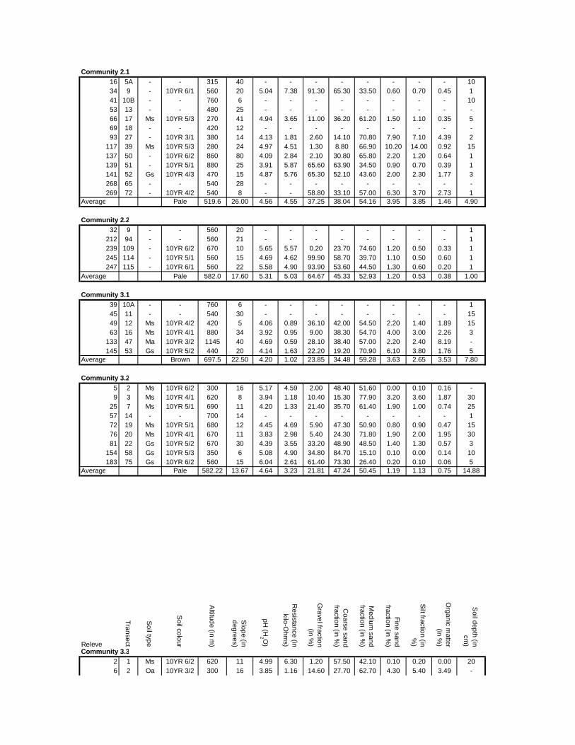
Community 2.116 5A - - 315 40 - - - - - - - - 1034 9 - 10YR 6/1 560 20 5.04 7.38 91.30 65.30 33.50 0.60 0.70 0.45 141 10B - - 760 6 - - - - - - - - 1053 13 - - 480 25 - - - - - - - - -66 17 Ms 10YR 5/3 270 41 4.94 3.65 11.00 36.20 61.20 1.50 1.10 0.35 569 18 - - 420 12 - - - - - - - - -93 27 - 10YR 3/1 380 14 4.13 1.81 2.60 14.10 70.80 7.90 7.10 4.39 2
117 39 Ms 10YR 5/3 280 24 4.97 4.51 1.30 8.80 66.90 10.20 14.00 0.92 15137 50 - 10YR 6/2 860 80 4.09 2.84 2.10 30.80 65.80 2.20 1.20 0.64 1139 51 - 10YR 5/1 880 25 3.91 5.87 65.60 63.90 34.50 0.90 0.70 0.39 1141 52 Gs 10YR 4/3 470 15 4.87 5.76 65.30 52.10 43.60 2.00 2.30 1.77 3268 65 - - 540 28 - - - - - - - - -269 72 - 10YR 4/2 540 8 - - 58.80 33.10 57.00 6.30 3.70 2.73 1
Average Pale 519.6 26.00 4.56 4.55 37.25 38.04 54.16 3.95 3.85 1.46 4.90
Community 2.232 9 - - 560 20 - - - - - - - - 1
212 94 - - 560 21 - - - - - - - - 1239 109 - 10YR 6/2 670 10 5.65 5.57 0.20 23.70 74.60 1.20 0.50 0.33 1245 114 - 10YR 5/1 560 15 4.69 4.62 99.90 58.70 39.70 1.10 0.50 0.60 1247 115 - 10YR 6/1 560 22 5.58 4.90 93.90 53.60 44.50 1.30 0.60 0.20 1
Average Pale 582.0 17.60 5.31 5.03 64.67 45.33 52.93 1.20 0.53 0.38 1.00
Community 3.139 10A - - 760 6 - - - - - - - - 145 11 - - 540 30 - - - - - - - - 1549 12 Ms 10YR 4/2 420 5 4.06 0.89 36.10 42.00 54.50 2.20 1.40 1.89 1563 16 Ms 10YR 4/1 880 34 3.92 0.95 9.00 38.30 54.70 4.00 3.00 2.26 3
133 47 Ma 10YR 3/2 1145 40 4.69 0.59 28.10 38.40 57.00 2.20 2.40 8.19 -145 53 Gs 10YR 5/2 440 20 4.14 1.63 22.20 19.20 70.90 6.10 3.80 1.76 5
Average Brown 697.5 22.50 4.20 1.02 23.85 34.48 59.28 3.63 2.65 3.53 7.80
Community 3.25 2 Ms 10YR 6/2 300 16 5.17 4.59 2.00 48.40 51.60 0.00 0.10 0.16 -9 3 Ms 10YR 4/1 620 8 3.94 1.18 10.40 15.30 77.90 3.20 3.60 1.87 30
25 7 Ms 10YR 5/1 690 11 4.20 1.33 21.40 35.70 61.40 1.90 1.00 0.74 2557 14 - - 700 14 - - - - - - - - 172 19 Ms 10YR 5/1 680 12 4.45 4.69 5.90 47.30 50.90 0.80 0.90 0.47 1576 20 Ms 10YR 4/1 670 11 3.83 2.98 5.40 24.30 71.80 1.90 2.00 1.95 3081 22 Gs 10YR 5/2 670 30 4.39 3.55 33.20 48.90 48.50 1.40 1.30 0.57 3
154 58 Gs 10YR 5/3 350 6 5.08 4.90 34.80 84.70 15.10 0.10 0.00 0.14 10183 75 Gs 10YR 6/2 560 15 6.04 2.61 61.40 73.30 26.40 0.20 0.10 0.06 5
Average Pale 582.22 13.67 4.64 3.23 21.81 47.24 50.45 1.19 1.13 0.75 14.88
Releve
Transect
Soil type
Soil colour
Altitude (in m
)
Slope (in
degrees)
pH (H
2 O)
Resistance (in
kilo-Ohm
s)
Gravel fraction
(in %)
Coarse sand
fraction (in %)
Medium
sand fraction (in %
)
Fine sand fraction (in %
)
Silt fraction (in
%)
Organic m
atter (in %
)
Soil depth (in
cm)
Community 3.32 1 Ms 10YR 6/2 620 11 4.99 6.30 1.20 57.50 42.10 0.10 0.20 0.00 206 2 Oa 10YR 3/2 300 16 3.85 1.16 14.60 27.70 62.70 4.30 5.40 3.49 -
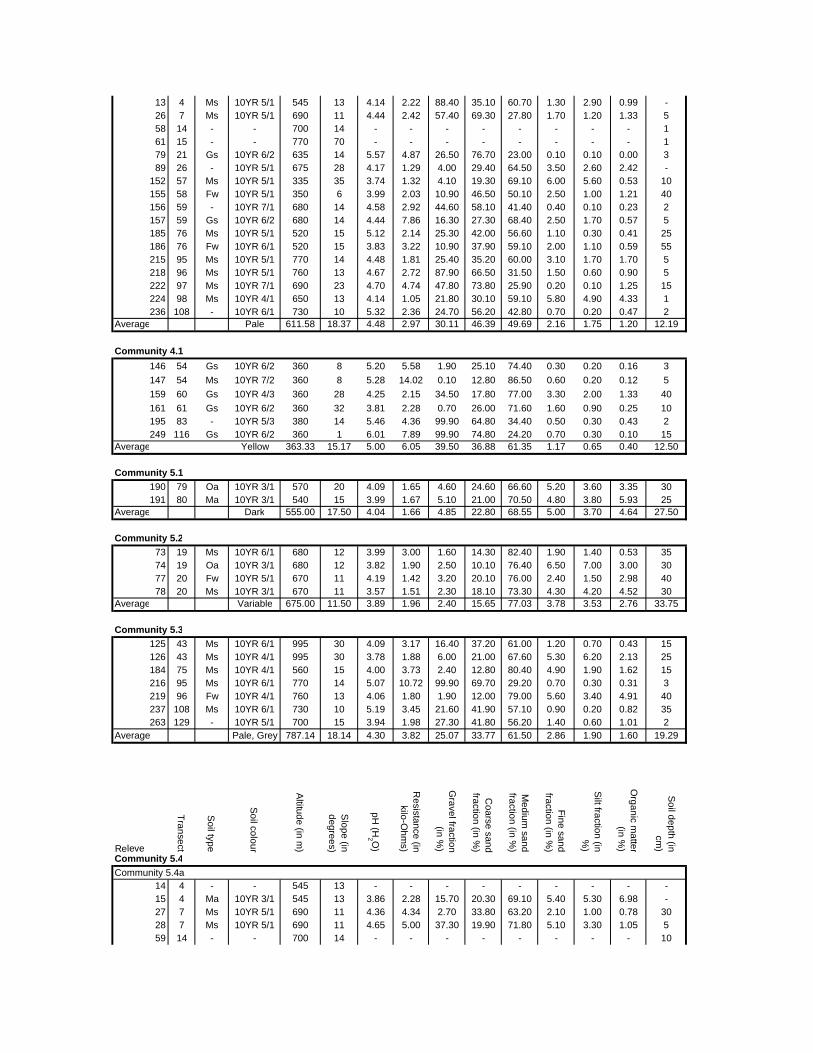
13 4 Ms 10YR 5/1 545 13 4.14 2.22 88.40 35.10 60.70 1.30 2.90 0.99 -26 7 Ms 10YR 5/1 690 11 4.44 2.42 57.40 69.30 27.80 1.70 1.20 1.33 558 14 - - 700 14 - - - - - - - - 161 15 - - 770 70 - - - - - - - - 179 21 Gs 10YR 6/2 635 14 5.57 4.87 26.50 76.70 23.00 0.10 0.10 0.00 389 26 - 10YR 5/1 675 28 4.17 1.29 4.00 29.40 64.50 3.50 2.60 2.42 -
152 57 Ms 10YR 5/1 335 35 3.74 1.32 4.10 19.30 69.10 6.00 5.60 0.53 10155 58 Fw 10YR 5/1 350 6 3.99 2.03 10.90 46.50 50.10 2.50 1.00 1.21 40156 59 - 10YR 7/1 680 14 4.58 2.92 44.60 58.10 41.40 0.40 0.10 0.23 2157 59 Gs 10YR 6/2 680 14 4.44 7.86 16.30 27.30 68.40 2.50 1.70 0.57 5185 76 Ms 10YR 5/1 520 15 5.12 2.14 25.30 42.00 56.60 1.10 0.30 0.41 25186 76 Fw 10YR 6/1 520 15 3.83 3.22 10.90 37.90 59.10 2.00 1.10 0.59 55215 95 Ms 10YR 5/1 770 14 4.48 1.81 25.40 35.20 60.00 3.10 1.70 1.70 5218 96 Ms 10YR 5/1 760 13 4.67 2.72 87.90 66.50 31.50 1.50 0.60 0.90 5222 97 Ms 10YR 7/1 690 23 4.70 4.74 47.80 73.80 25.90 0.20 0.10 1.25 15224 98 Ms 10YR 4/1 650 13 4.14 1.05 21.80 30.10 59.10 5.80 4.90 4.33 1236 108 - 10YR 6/1 730 10 5.32 2.36 24.70 56.20 42.80 0.70 0.20 0.47 2
Average Pale 611.58 18.37 4.48 2.97 30.11 46.39 49.69 2.16 1.75 1.20 12.19
Community 4.1146 54 Gs 10YR 6/2 360 8 5.20 5.58 1.90 25.10 74.40 0.30 0.20 0.16 3147 54 Ms 10YR 7/2 360 8 5.28 14.02 0.10 12.80 86.50 0.60 0.20 0.12 5159 60 Gs 10YR 4/3 360 28 4.25 2.15 34.50 17.80 77.00 3.30 2.00 1.33 40161 61 Gs 10YR 6/2 360 32 3.81 2.28 0.70 26.00 71.60 1.60 0.90 0.25 10195 83 - 10YR 5/3 380 14 5.46 4.36 99.90 64.80 34.40 0.50 0.30 0.43 2249 116 Gs 10YR 6/2 360 1 6.01 7.89 99.90 74.80 24.20 0.70 0.30 0.10 15
Average Yellow 363.33 15.17 5.00 6.05 39.50 36.88 61.35 1.17 0.65 0.40 12.50
Community 5.1190 79 Oa 10YR 3/1 570 20 4.09 1.65 4.60 24.60 66.60 5.20 3.60 3.35 30191 80 Ma 10YR 3/1 540 15 3.99 1.67 5.10 21.00 70.50 4.80 3.80 5.93 25
Average Dark 555.00 17.50 4.04 1.66 4.85 22.80 68.55 5.00 3.70 4.64 27.50
Community 5.273 19 Ms 10YR 6/1 680 12 3.99 3.00 1.60 14.30 82.40 1.90 1.40 0.53 3574 19 Oa 10YR 3/1 680 12 3.82 1.90 2.50 10.10 76.40 6.50 7.00 3.00 3077 20 Fw 10YR 5/1 670 11 4.19 1.42 3.20 20.10 76.00 2.40 1.50 2.98 4078 20 Ms 10YR 3/1 670 11 3.57 1.51 2.30 18.10 73.30 4.30 4.20 4.52 30
Average Variable 675.00 11.50 3.89 1.96 2.40 15.65 77.03 3.78 3.53 2.76 33.75
Community 5.3125 43 Ms 10YR 6/1 995 30 4.09 3.17 16.40 37.20 61.00 1.20 0.70 0.43 15126 43 Ms 10YR 4/1 995 30 3.78 1.88 6.00 21.00 67.60 5.30 6.20 2.13 25184 75 Ms 10YR 4/1 560 15 4.00 3.73 2.40 12.80 80.40 4.90 1.90 1.62 15216 95 Ms 10YR 6/1 770 14 5.07 10.72 99.90 69.70 29.20 0.70 0.30 0.31 3219 96 Fw 10YR 4/1 760 13 4.06 1.80 1.90 12.00 79.00 5.60 3.40 4.91 40237 108 Ms 10YR 6/1 730 10 5.19 3.45 21.60 41.90 57.10 0.90 0.20 0.82 35263 129 - 10YR 5/1 700 15 3.94 1.98 27.30 41.80 56.20 1.40 0.60 1.01 2
Average Pale, Grey 787.14 18.14 4.30 3.82 25.07 33.77 61.50 2.86 1.90 1.60 19.29
Releve
Transect
Soil type
Soil colour
Altitude (in m
)
Slope (in
degrees)
pH (H
2 O)
Resistance (in
kilo-Ohm
s)
Gravel fraction
(in %)
Coarse sand
fraction (in %)
Medium
sand fraction (in %
)
Fine sand fraction (in %
)
Silt fraction (in
%)
Organic m
atter (in %
)
Soil depth (in
cm)
Community 5.4Community 5.4a
14 4 - - 545 13 - - - - - - - - -15 4 Ma 10YR 3/1 545 13 3.86 2.28 15.70 20.30 69.10 5.40 5.30 6.98 -27 7 Ms 10YR 5/1 690 11 4.36 4.34 2.70 33.80 63.20 2.10 1.00 0.78 3028 7 Ms 10YR 5/1 690 11 4.65 5.00 37.30 19.90 71.80 5.10 3.30 1.05 559 14 - - 700 14 - - - - - - - - 10
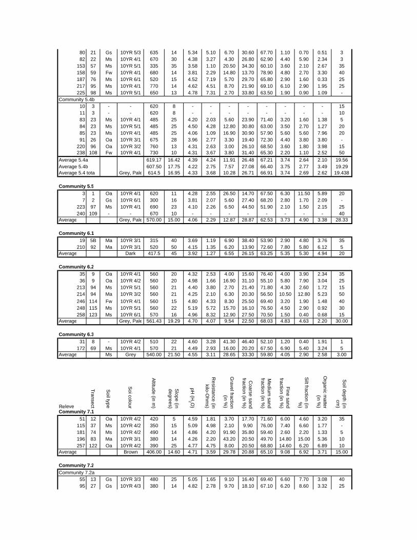
80 21 Gs 10YR 5/3 635 14 5.34 5.10 6.70 30.60 67.70 1.10 0.70 0.51 382 22 Ms 10YR 4/1 670 30 4.38 3.27 4.30 26.80 62.90 4.40 5.90 2.34 3
153 57 Ms 10YR 5/1 335 35 3.58 1.10 20.50 34.30 60.10 3.60 2.10 2.67 35158 59 Fw 10YR 4/1 680 14 3.81 2.29 14.80 13.70 78.90 4.80 2.70 3.30 40187 76 Ms 10YR 6/1 520 15 4.52 7.19 5.70 29.70 65.80 2.90 1.60 0.33 25217 95 Ms 10YR 4/1 770 14 4.62 4.51 8.70 21.90 69.10 6.10 2.90 1.95 25225 98 Ms 10YR 5/1 650 13 4.78 7.31 2.70 33.80 63.50 1.90 0.90 1.09 -
Community 5.4b10 3 - - 620 8 - - - - - - - - 1511 3 - - 620 8 - - - - - - - - 1083 23 Ms 10YR 4/1 485 25 4.20 2.03 5.60 23.90 71.40 3.20 1.60 1.38 584 23 Ms 10YR 5/1 485 25 4.50 4.28 12.80 30.80 63.00 3.50 2.70 1.27 2085 23 Ms 10YR 4/1 485 25 4.06 1.09 16.90 30.90 57.90 5.60 5.60 7.96 2091 26 Oa 10YR 3/1 675 28 3.96 2.77 3.30 19.40 72.30 4.40 3.80 3.80 -
220 96 Oa 10YR 3/2 760 13 4.31 2.63 3.00 26.10 68.50 3.60 1.80 3.98 15238 108 Fw 10YR 4/1 730 10 4.31 3.67 3.80 31.40 65.30 2.20 1.10 2.52 50
Average 5.4a 619.17 16.42 4.39 4.24 11.91 26.48 67.21 3.74 2.64 2.10 19.56Average 5.4b 607.50 17.75 4.22 2.75 7.57 27.08 66.40 3.75 2.77 3.49 19.29Average 5.4 tota Grey, Pale 614.5 16.95 4.33 3.68 10.28 26.71 66.91 3.74 2.69 2.62 19.438
Community 5.53 1 Oa 10YR 4/1 620 11 4.28 2.55 26.50 14.70 67.50 6.30 11.50 5.89 207 2 Gs 10YR 6/1 300 16 3.81 2.07 5.60 27.40 68.20 2.80 1.70 2.09 -
223 97 Ms 10YR 4/1 690 23 4.10 2.26 6.50 44.50 51.90 2.10 1.50 2.15 25240 109 - - 670 10 - - - - - - - - 40
Average Grey, Pale 570.00 15.00 4.06 2.29 12.87 28.87 62.53 3.73 4.90 3.38 28.33
Community 6.119 5B Ma 10YR 3/1 315 40 3.69 1.19 6.90 38.40 53.90 2.90 4.80 3.76 35
210 92 Ma 10YR 3/1 520 50 4.15 1.35 6.20 13.90 72.60 7.80 5.80 6.12 5Average Dark 417.5 45 3.92 1.27 6.55 26.15 63.25 5.35 5.30 4.94 20
Community 6.235 9 Oa 10YR 4/1 560 20 4.32 2.53 4.00 15.60 76.40 4.00 3.90 2.34 3536 9 Oa 10YR 4/2 560 20 4.98 1.66 16.90 31.10 55.10 5.80 7.90 3.04 25
213 94 Ms 10YR 5/1 560 21 4.40 3.80 2.70 21.40 71.80 4.30 2.60 1.72 15214 94 Ma 10YR 3/2 560 21 4.25 2.10 6.30 20.30 56.50 10.50 12.80 5.23 50246 114 Fw 10YR 4/1 560 15 4.80 4.33 8.30 25.50 69.40 3.20 1.90 1.48 40248 115 Ms 10YR 5/1 560 22 5.19 5.72 15.70 16.10 76.50 4.50 2.90 0.92 30258 123 Ms 10YR 6/1 570 16 4.96 8.32 12.90 27.50 70.50 1.50 0.40 0.68 15
Average Grey, Pale 561.43 19.29 4.70 4.07 9.54 22.50 68.03 4.83 4.63 2.20 30.00
Community 6.331 8 - 10YR 4/2 510 22 4.60 3.28 41.30 46.40 52.10 1.20 0.40 1.91 1
172 69 Ms 10YR 4/1 570 21 4.49 2.93 16.00 20.20 67.50 6.90 5.40 3.24 5Average Ms Grey 540.00 21.50 4.55 3.11 28.65 33.30 59.80 4.05 2.90 2.58 3.00
Releve
Transect
Soil type
Soi colour
Altitude (in m
)
Slope (in
degrees)
pH (H
2 O)
Resistance (in
kilo-Ohm
s)
Gravel fraction
(in %)
Coarse sand
fraction (in %)
Medium
sand fraction (in %
)
Fine sand fraction (in %
)
Silt fraction (in
%)
Organic m
atter (in %
)
Soil depth (in
cm)
Community 7.151 12 Oa 10YR 4/2 420 5 4.59 1.81 3.70 17.70 71.60 6.00 4.60 3.20 35
115 37 Ms 10YR 4/2 350 15 5.09 4.98 2.10 9.90 76.00 7.40 6.60 1.77 -181 74 Ms 10YR 4/2 490 14 4.86 4.20 91.90 35.80 59.40 2.60 2.20 1.33 5196 83 Ma 10YR 3/1 380 14 4.26 2.20 43.20 20.50 49.70 14.80 15.00 5.36 10257 122 Oa 10YR 4/2 390 25 4.77 4.75 8.00 20.50 68.80 14.60 6.20 6.89 10
Average Brown 406.00 14.60 4.71 3.59 29.78 20.88 65.10 9.08 6.92 3.71 15.00
Community 7.2Community 7.2a
55 13 Gs 10YR 3/3 480 25 5.05 1.65 9.10 16.40 69.40 6.60 7.70 3.08 4095 27 Gs 10YR 4/3 380 14 4.82 2.78 9.70 18.10 67.10 6.20 8.60 3.32 25
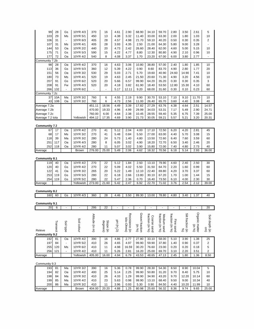
99 28 Gs 10YR 4/3 370 16 4.61 2.90 68.90 34.10 59.70 2.80 3.50 2.61 5103 29 Ms 10YR 5/1 450 13 4.38 3.32 11.40 33.00 63.30 2.00 1.80 1.03 10106 31 - 10YR 6/3 405 28 4.57 4.98 21.70 59.10 40.20 0.50 0.30 0.35 2107 31 Ms 10YR 4/1 405 28 3.93 4.35 2.50 21.00 64.30 5.80 9.00 3.28 -144 53 Oa 10YR 2/2 440 20 4.73 2.42 26.60 28.40 62.00 4.60 5.00 5.15 10175 71 Gs 10YR 5/3 590 15 4.22 4.77 8.80 12.30 80.80 4.90 2.10 0.96 10177 72 Oa 10YR 4/2 540 8 4.08 3.37 1.70 23.20 67.00 6.00 3.80 2.77 -
Community 7.2b98 28 Oa 10YR 4/2 370 16 4.63 3.06 10.80 38.80 57.00 2.40 1.80 1.85 10
113 36 Gs 10YR 5/3 360 12 5.39 4.22 0.90 8.60 83.70 4.90 2.80 1.77 20151 56 Oa 10YR 3/2 530 29 5.03 2.71 5.70 19.60 40.90 24.60 14.90 7.41 10180 73 Ms 10YR 4/1 520 19 4.63 2.45 21.50 20.60 71.30 4.90 3.20 4.56 10207 91 Gs 10YR 6/2 520 20 5.66 6.57 99.90 64.20 35.20 0.30 0.30 0.35 3208 91 Fw 10YR 4/3 520 20 4.18 3.82 61.90 18.40 53.50 12.80 15.30 4.10 60266 132 - 10YR 6/2 - - 5.17 12.11 9.20 68.00 31.60 0.30 0.10 0.23 60
Community 7.2c37 10A Ma 10YR 3/2 760 6 4.55 2.19 9.90 30.70 53.10 7.10 9.10 11.70 1043 10B Oa 10YR 3/2 760 6 4.73 2.56 11.00 26.40 65.70 3.60 4.40 3.08 40
Average 7.2a 451.11 18.56 4.49 3.39 17.82 27.29 63.76 4.38 4.64 2.51 14.57Average 7.2b 470.00 19.33 4.96 4.99 29.99 34.03 53.31 7.17 5.49 2.90 24.71Average 7.2c 760.00 6.00 4.64 2.38 10.45 28.55 59.40 5.35 6.75 7.39 25.00Average 7.2 tota Yellowish 494.12 17.35 4.69 3.90 21.73 30.05 59.21 5.57 5.21 3.20 20.31
Community 7.367 17 Oa 10YR 4/2 270 41 5.12 2.04 4.00 17.10 72.50 6.20 4.20 2.81 4568 17 Ms 10YR 3/2 270 41 5.48 0.84 5.50 27.00 63.00 4.40 5.70 3.08 15
118 39 Ma 10YR 3/2 280 24 5.73 1.40 4.80 13.50 72.60 6.40 7.60 3.59 60251 117 Oa 10YR 4/3 280 8 6.05 3.02 4.90 18.20 72.70 6.50 3.40 2.46 20252 118 Oa 10YR 4/2 280 11 5.07 3.02 3.90 15.80 72.00 7.40 4.80 2.73 40
Average Brown 276.00 25.00 5.49 2.06 4.62 18.32 70.56 6.18 5.14 2.93 36.00
Community 8.1119 40 Oa 10YR 4/2 270 22 5.12 1.84 2.50 13.10 79.90 4.60 2.40 2.50 30120 40 Gs 10YR 4/2 270 22 5.09 4.02 5.50 31.50 64.70 2.20 1.60 0.99 60122 41 Oa 10YR 3/2 265 20 5.22 1.49 12.10 22.40 69.80 4.20 3.70 3.37 60253 119 Gs 10YR 5/3 280 22 6.18 2.66 13.80 30.10 67.20 1.70 1.00 1.44 15254 119 Gs 10YR 5/2 280 22 5.47 2.36 0.70 16.40 73.50 6.10 4.00 2.30 30
Average Yellowish 273.00 21.60 5.42 2.47 6.92 22.70 71.02 3.76 2.54 2.12 39.00
Community 8.2160 60 Gs 10YR 4/3 360 28 4.46 3.50 89.30 13.00 78.80 4.80 3.40 1.37 40
Community 9.120 6 - - 295 22 - - - - - - - - 20
Releve
Transect
Soil type
Soil colour
Altitude (in m
)
Slope (in
degrees)
pH (H
2 O)
Resistance (in
kilo-Ohm
s)
Gravel fraction
(in %)
Coarse sand
fraction (in %)
Medium
sand fraction (in %
)
Fine sand fraction (in %
)
Silt fraction (in
%)
Organic m
atter (in %
)
Soil depth (in
cm)
Community 9.2192 81 Oa 10YR 4/2 390 16 4.86 2.77 27.80 33.10 58.00 5.10 3.90 1.38 25197 84 - 10YR 5/2 410 26 4.65 4.97 99.90 59.90 37.80 1.40 0.90 0.37 2255 120 Ms 10YR 6/2 410 11 4.98 16.59 30.20 76.60 23.00 0.20 0.20 0.18 5256 121 - 10YR 4/2 410 11 5.26 2.81 16.20 25.00 69.70 3.10 2.20 3.51 2
Average Yellowish 405.00 16.00 4.94 6.79 43.53 48.65 47.13 2.45 1.80 1.36 8.50
Community 9.3193 81 Ma 10YR 3/2 390 16 5.36 0.78 99.90 28.30 54.30 8.50 8.90 10.04 5194 82 Oa 10YR 4/2 400 25 5.14 2.25 99.90 50.80 31.20 9.70 8.40 5.75 10198 84 Ma 10YR 3/2 410 26 4.33 1.29 99.90 34.90 43.20 9.70 12.20 10.14 60199 85 Ma 10YR 4/2 410 23 5.63 0.98 99.90 13.10 68.40 9.50 9.00 10.34 40200 86 Ma 10YR 3/2 410 11 3.96 0.93 5.30 0.90 84.50 4.40 10.20 11.99 10
Average Brown 404.00 20.20 4.88 1.25 80.98 25.60 56.32 8.36 9.74 9.65 25.00
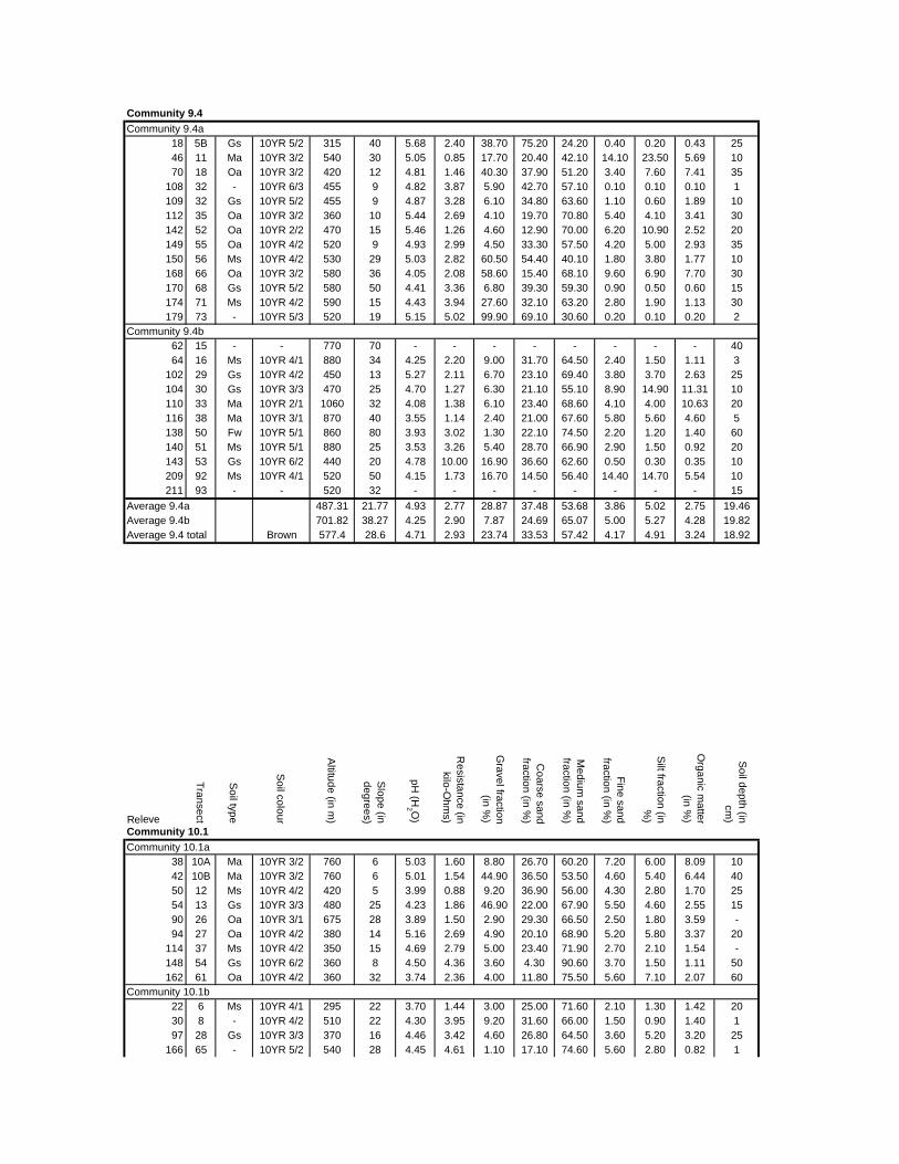
Community 9.4Community 9.4a
18 5B Gs 10YR 5/2 315 40 5.68 2.40 38.70 75.20 24.20 0.40 0.20 0.43 2546 11 Ma 10YR 3/2 540 30 5.05 0.85 17.70 20.40 42.10 14.10 23.50 5.69 1070 18 Oa 10YR 3/2 420 12 4.81 1.46 40.30 37.90 51.20 3.40 7.60 7.41 35
108 32 - 10YR 6/3 455 9 4.82 3.87 5.90 42.70 57.10 0.10 0.10 0.10 1109 32 Gs 10YR 5/2 455 9 4.87 3.28 6.10 34.80 63.60 1.10 0.60 1.89 10112 35 Oa 10YR 3/2 360 10 5.44 2.69 4.10 19.70 70.80 5.40 4.10 3.41 30142 52 Oa 10YR 2/2 470 15 5.46 1.26 4.60 12.90 70.00 6.20 10.90 2.52 20149 55 Oa 10YR 4/2 520 9 4.93 2.99 4.50 33.30 57.50 4.20 5.00 2.93 35150 56 Ms 10YR 4/2 530 29 5.03 2.82 60.50 54.40 40.10 1.80 3.80 1.77 10168 66 Oa 10YR 3/2 580 36 4.05 2.08 58.60 15.40 68.10 9.60 6.90 7.70 30170 68 Gs 10YR 5/2 580 50 4.41 3.36 6.80 39.30 59.30 0.90 0.50 0.60 15174 71 Ms 10YR 4/2 590 15 4.43 3.94 27.60 32.10 63.20 2.80 1.90 1.13 30179 73 - 10YR 5/3 520 19 5.15 5.02 99.90 69.10 30.60 0.20 0.10 0.20 2
Community 9.4b62 15 - - 770 70 - - - - - - - - 4064 16 Ms 10YR 4/1 880 34 4.25 2.20 9.00 31.70 64.50 2.40 1.50 1.11 3
102 29 Gs 10YR 4/2 450 13 5.27 2.11 6.70 23.10 69.40 3.80 3.70 2.63 25104 30 Gs 10YR 3/3 470 25 4.70 1.27 6.30 21.10 55.10 8.90 14.90 11.31 10110 33 Ma 10YR 2/1 1060 32 4.08 1.38 6.10 23.40 68.60 4.10 4.00 10.63 20116 38 Ma 10YR 3/1 870 40 3.55 1.14 2.40 21.00 67.60 5.80 5.60 4.60 5138 50 Fw 10YR 5/1 860 80 3.93 3.02 1.30 22.10 74.50 2.20 1.20 1.40 60140 51 Ms 10YR 5/1 880 25 3.53 3.26 5.40 28.70 66.90 2.90 1.50 0.92 20143 53 Gs 10YR 6/2 440 20 4.78 10.00 16.90 36.60 62.60 0.50 0.30 0.35 10209 92 Ms 10YR 4/1 520 50 4.15 1.73 16.70 14.50 56.40 14.40 14.70 5.54 10211 93 - - 520 32 - - - - - - - - 15
Average 9.4a 487.31 21.77 4.93 2.77 28.87 37.48 53.68 3.86 5.02 2.75 19.46Average 9.4b 701.82 38.27 4.25 2.90 7.87 24.69 65.07 5.00 5.27 4.28 19.82Average 9.4 total Brown 577.4 28.6 4.71 2.93 23.74 33.53 57.42 4.17 4.91 3.24 18.92
Releve
Transect
Soil type
Soil colour
Altitude (in m
)
Slope (in
degrees)
pH (H
2 O)
Resistance (in
kilo-Ohm
s)
Gravel fraction
(in %)
Coarse sand
fraction (in %)
Medium
sand fraction (in %
)
Fine sand fraction (in %
)
Silt fraction (in
%)
Organic m
atter (in %
)
Soil depth (in
cm)
Community 10.1Community 10.1a
38 10A Ma 10YR 3/2 760 6 5.03 1.60 8.80 26.70 60.20 7.20 6.00 8.09 1042 10B Ma 10YR 3/2 760 6 5.01 1.54 44.90 36.50 53.50 4.60 5.40 6.44 4050 12 Ms 10YR 4/2 420 5 3.99 0.88 9.20 36.90 56.00 4.30 2.80 1.70 2554 13 Gs 10YR 3/3 480 25 4.23 1.86 46.90 22.00 67.90 5.50 4.60 2.55 1590 26 Oa 10YR 3/1 675 28 3.89 1.50 2.90 29.30 66.50 2.50 1.80 3.59 -94 27 Oa 10YR 4/2 380 14 5.16 2.69 4.90 20.10 68.90 5.20 5.80 3.37 20
114 37 Ms 10YR 4/2 350 15 4.69 2.79 5.00 23.40 71.90 2.70 2.10 1.54 -148 54 Gs 10YR 6/2 360 8 4.50 4.36 3.60 4.30 90.60 3.70 1.50 1.11 50162 61 Oa 10YR 4/2 360 32 3.74 2.36 4.00 11.80 75.50 5.60 7.10 2.07 60
Community 10.1b22 6 Ms 10YR 4/1 295 22 3.70 1.44 3.00 25.00 71.60 2.10 1.30 1.42 2030 8 - 10YR 4/2 510 22 4.30 3.95 9.20 31.60 66.00 1.50 0.90 1.40 197 28 Gs 10YR 3/3 370 16 4.46 3.42 4.60 26.80 64.50 3.60 5.20 3.20 25
166 65 - 10YR 5/2 540 28 4.45 4.61 1.10 17.10 74.60 5.60 2.80 0.82 1

169 67 - 10YR 4/2 570 18 4.96 2.50 99.90 51.10 47.60 0.80 0.40 0.72 1171 69 - 10YR 4/2 570 21 4.15 4.07 99.90 48.70 48.10 1.80 1.50 1.03 1176 72 - 10YR 4/2 540 8 4.12 2.97 58.80 33.10 57.00 6.30 3.70 2.73 1206 91 Gs 10YR 6/3 520 20 4.51 2.63 7.30 36.30 60.60 2.20 0.90 0.29 3265 131 - 10YR 6/2 - - 4.48 5.02 14.20 28.30 65.20 4.80 1.70 1.60 2
Average 10.1a 505.00 15.44 4.47 2.18 14.47 23.44 67.89 4.59 4.12 3.38 31.43Average 10.1b 489.38 19.38 4.35 3.40 33.11 33.11 61.69 3.19 2.04 1.47 6.11Average 10.1 tot. Brown 497.65 17.29 4.41 2.79 23.79 28.28 64.79 3.89 3.08 2.43 17.19
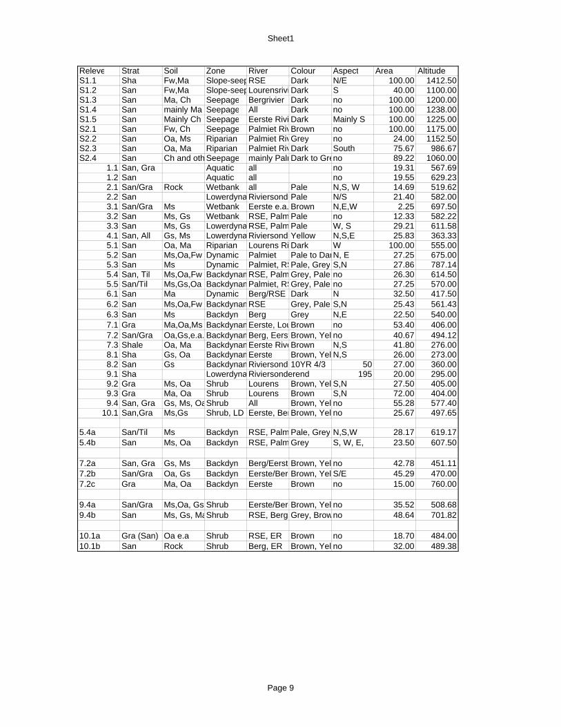
Sheet1
Releve Strat Soil Zone River Colour Aspect Area AltitudeS1.1 Sha Fw,Ma Slope-seepRSE Dark N/E 100.00 1412.50S1.2 San Fw,Ma Slope-seepLourensrivi Dark S 40.00 1100.00S1.3 San Ma, Ch Seepage Bergrivier Dark no 100.00 1200.00S1.4 San mainly Ma Seepage All Dark no 100.00 1238.00S1.5 San Mainly Ch Seepage Eerste Rivi Dark Mainly S 100.00 1225.00S2.1 San Fw, Ch Seepage Palmiet RivBrown no 100.00 1175.00S2.2 San Oa, Ms Riparian Palmiet RivGrey no 24.00 1152.50S2.3 San Oa, Ma Riparian Palmiet RivDark South 75.67 986.67S2.4 San Ch and oth Seepage mainly PalmDark to Greno 89.22 1060.00
1.1 San, Gra Aquatic all no 19.31 567.691.2 San Aquatic all no 19.55 629.232.1 San/Gra Rock Wetbank all Pale N,S, W 14.69 519.622.2 San Lowerdyna RiviersondePale N/S 21.40 582.003.1 San/Gra Ms Wetbank Eerste e.a. Brown N,E,W 2.25 697.503.2 San Ms, Gs Wetbank RSE, Palm Pale no 12.33 582.223.3 San Ms, Gs Lowerdyna RSE, Palm Pale W, S 29.21 611.584.1 San, All Gs, Ms Lowerdyna RiviersondeYellow N,S,E 25.83 363.335.1 San Oa, Ma Riparian Lourens Ri Dark W 100.00 555.005.2 San Ms,Oa,Fw Dynamic Palmiet Pale to DarN, E 27.25 675.005.3 San Ms Dynamic Palmiet, RSPale, Grey S,N 27.86 787.145.4 San, Til Ms,Oa,Fw BackdynamRSE, Palm Grey, Pale no 26.30 614.505.5 San/Til Ms,Gs,Oa BackdynamPalmiet, RSGrey, Pale no 27.25 570.006.1 San Ma Dynamic Berg/RSE Dark N 32.50 417.506.2 San Ms,Oa,Fw BackdynamRSE Grey, Pale S,N 25.43 561.436.3 San Ms Backdyn Berg Grey N,E 22.50 540.007.1 Gra Ma,Oa,Ms BackdynamEerste, LouBrown no 53.40 406.007.2 San/Gra Oa,Gs,e.a. BackdynamBerg, EerstBrown, Yel no 40.67 494.127.3 Shale Oa, Ma BackdynamEerste RiveBrown N,S 41.80 276.008.1 Sha Gs, Oa BackdynamEerste Brown, Yel N,S 26.00 273.008.2 San Gs BackdynamRiviersonde10YR 4/3 50 27.00 360.009.1 Sha Lowerdyna Riviersonderend 195 20.00 295.009.2 Gra Ms, Oa Shrub Lourens Brown, Yel S,N 27.50 405.009.3 Gra Ma, Oa Shrub Lourens Brown S,N 72.00 404.009.4 San, Gra Gs, Ms, OaShrub All Brown, Yel no 55.28 577.40
10.1 San,Gra Ms,Gs Shrub, LD Eerste, BerBrown, Yel no 25.67 497.65
5.4a San/Til Ms Backdyn RSE, Palm Pale, Grey N,S,W 28.17 619.175.4b San Ms, Oa Backdyn RSE, Palm Grey S, W, E, 23.50 607.50
7.2a San, Gra Gs, Ms Backdyn Berg/EersteBrown, Yel no 42.78 451.117.2b San/Gra Oa, Gs Backdyn Eerste/BergBrown, Yel S/E 45.29 470.007.2c Gra Ma, Oa Backdyn Eerste Brown no 15.00 760.00
9.4a San/Gra Ms,Oa, Gs Shrub Eerste/BergBrown, Yel no 35.52 508.689.4b San Ms, Gs, MaShrub RSE, Berg Grey, Browno 48.64 701.82
10.1a Gra (San) Oa e.a Shrub RSE, ER Brown no 18.70 484.0010.1b San Rock Shrub Berg, ER Brown, Yel no 32.00 489.38
Page 9
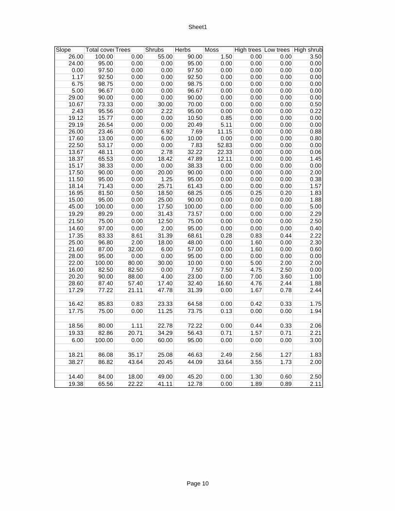
Sheet1
Slope Total coverTrees Shrubs Herbs Moss High trees Low trees High shrub26.00 100.00 0.00 55.00 90.00 1.50 0.00 0.00 3.5024.00 95.00 0.00 0.00 95.00 0.00 0.00 0.00 0.000.00 97.50 0.00 0.00 97.50 0.00 0.00 0.00 0.001.17 92.50 0.00 0.00 92.50 0.00 0.00 0.00 0.006.75 98.75 0.00 0.00 98.75 0.00 0.00 0.00 0.005.00 96.67 0.00 0.00 96.67 0.00 0.00 0.00 0.00
29.00 90.00 0.00 0.00 90.00 0.00 0.00 0.00 0.0010.67 73.33 0.00 30.00 70.00 0.00 0.00 0.00 0.502.43 95.56 0.00 2.22 95.00 0.00 0.00 0.00 0.22
19.12 15.77 0.00 0.00 10.50 0.85 0.00 0.00 0.0029.19 26.54 0.00 0.00 20.49 5.11 0.00 0.00 0.0026.00 23.46 0.00 6.92 7.69 11.15 0.00 0.00 0.8817.60 13.00 0.00 6.00 10.00 0.00 0.00 0.00 0.8022.50 53.17 0.00 0.00 7.83 52.83 0.00 0.00 0.0013.67 48.11 0.00 2.78 32.22 22.33 0.00 0.00 0.0618.37 65.53 0.00 18.42 47.89 12.11 0.00 0.00 1.4515.17 38.33 0.00 0.00 38.33 0.00 0.00 0.00 0.0017.50 90.00 0.00 20.00 90.00 0.00 0.00 0.00 2.0011.50 95.00 0.00 1.25 95.00 0.00 0.00 0.00 0.3818.14 71.43 0.00 25.71 61.43 0.00 0.00 0.00 1.5716.95 81.50 0.50 18.50 68.25 0.05 0.25 0.20 1.8315.00 95.00 0.00 25.00 90.00 0.00 0.00 0.00 1.8845.00 100.00 0.00 17.50 100.00 0.00 0.00 0.00 5.0019.29 89.29 0.00 31.43 73.57 0.00 0.00 0.00 2.2921.50 75.00 0.00 12.50 75.00 0.00 0.00 0.00 2.5014.60 97.00 0.00 2.00 95.00 0.00 0.00 0.00 0.4017.35 83.33 8.61 31.39 68.61 0.28 0.83 0.44 2.2225.00 96.80 2.00 18.00 48.00 0.00 1.60 0.00 2.3021.60 87.00 32.00 6.00 57.00 0.00 1.60 0.00 0.6028.00 95.00 0.00 0.00 95.00 0.00 0.00 0.00 0.0022.00 100.00 80.00 30.00 10.00 0.00 5.00 2.00 2.0016.00 82.50 82.50 0.00 7.50 7.50 4.75 2.50 0.0020.20 90.00 88.00 4.00 23.00 0.00 7.00 3.60 1.0028.60 87.40 57.40 17.40 32.40 16.60 4.76 2.44 1.8817.29 77.22 21.11 47.78 31.39 0.00 1.67 0.78 2.44
16.42 85.83 0.83 23.33 64.58 0.00 0.42 0.33 1.7517.75 75.00 0.00 11.25 73.75 0.13 0.00 0.00 1.94
18.56 80.00 1.11 22.78 72.22 0.00 0.44 0.33 2.0619.33 82.86 20.71 34.29 56.43 0.71 1.57 0.71 2.216.00 100.00 0.00 60.00 95.00 0.00 0.00 0.00 3.00
18.21 86.08 35.17 25.08 46.63 2.49 2.56 1.27 1.8338.27 86.82 43.64 20.45 44.09 33.64 3.55 1.73 2.00
14.40 84.00 18.00 49.00 45.20 0.00 1.30 0.60 2.5019.38 65.56 22.22 41.11 12.78 0.00 1.89 0.89 2.11
Page 10
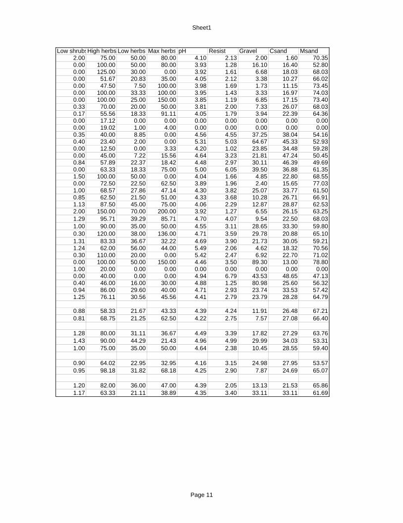
Sheet1
Low shrubsHigh herbs Low herbs Max herbs pH Resist Gravel Csand Msand2.00 75.00 50.00 80.00 4.10 2.13 2.00 1.60 70.350.00 100.00 50.00 80.00 3.93 1.28 16.10 16.40 52.800.00 125.00 30.00 0.00 3.92 1.61 6.68 18.03 68.030.00 51.67 20.83 35.00 4.05 2.12 3.38 10.27 66.020.00 47.50 7.50 100.00 3.98 1.69 1.73 11.15 73.450.00 100.00 33.33 100.00 3.95 1.43 3.33 16.97 74.030.00 100.00 25.00 150.00 3.85 1.19 6.85 17.15 73.400.33 70.00 20.00 50.00 3.81 2.00 7.33 26.07 68.030.17 55.56 18.33 91.11 4.05 1.79 3.94 22.39 64.360.00 17.12 0.00 0.00 0.00 0.00 0.00 0.00 0.000.00 19.02 1.00 4.00 0.00 0.00 0.00 0.00 0.000.35 40.00 8.85 0.00 4.56 4.55 37.25 38.04 54.160.40 23.40 2.00 0.00 5.31 5.03 64.67 45.33 52.930.00 12.50 0.00 3.33 4.20 1.02 23.85 34.48 59.280.00 45.00 7.22 15.56 4.64 3.23 21.81 47.24 50.450.84 57.89 22.37 18.42 4.48 2.97 30.11 46.39 49.690.00 63.33 18.33 75.00 5.00 6.05 39.50 36.88 61.351.50 100.00 50.00 0.00 4.04 1.66 4.85 22.80 68.550.00 72.50 22.50 62.50 3.89 1.96 2.40 15.65 77.031.00 68.57 27.86 47.14 4.30 3.82 25.07 33.77 61.500.85 62.50 21.50 51.00 4.33 3.68 10.28 26.71 66.911.13 87.50 45.00 75.00 4.06 2.29 12.87 28.87 62.532.00 150.00 70.00 200.00 3.92 1.27 6.55 26.15 63.251.29 95.71 39.29 85.71 4.70 4.07 9.54 22.50 68.031.00 90.00 35.00 50.00 4.55 3.11 28.65 33.30 59.800.30 120.00 38.00 136.00 4.71 3.59 29.78 20.88 65.101.31 83.33 36.67 32.22 4.69 3.90 21.73 30.05 59.211.24 62.00 56.00 44.00 5.49 2.06 4.62 18.32 70.560.30 110.00 20.00 0.00 5.42 2.47 6.92 22.70 71.020.00 100.00 50.00 150.00 4.46 3.50 89.30 13.00 78.801.00 20.00 0.00 0.00 0.00 0.00 0.00 0.00 0.000.00 40.00 0.00 0.00 4.94 6.79 43.53 48.65 47.130.40 46.00 16.00 30.00 4.88 1.25 80.98 25.60 56.320.94 86.00 29.60 40.00 4.71 2.93 23.74 33.53 57.421.25 76.11 30.56 45.56 4.41 2.79 23.79 28.28 64.79
0.88 58.33 21.67 43.33 4.39 4.24 11.91 26.48 67.210.81 68.75 21.25 62.50 4.22 2.75 7.57 27.08 66.40
1.28 80.00 31.11 36.67 4.49 3.39 17.82 27.29 63.761.43 90.00 44.29 21.43 4.96 4.99 29.99 34.03 53.311.00 75.00 35.00 50.00 4.64 2.38 10.45 28.55 59.40
0.90 64.02 22.95 32.95 4.16 3.15 24.98 27.95 53.570.95 98.18 31.82 68.18 4.25 2.90 7.87 24.69 65.07
1.20 82.00 36.00 47.00 4.39 2.05 13.13 21.53 65.861.17 63.33 21.11 38.89 4.35 3.40 33.11 33.11 61.69
Page 11
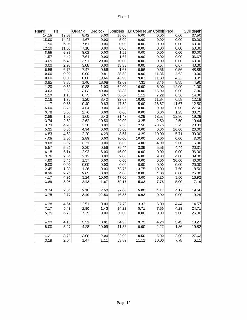
Sheet1
Fsand silt Organic Bedrock Boulders Lg CobblesSm CobblePebb SOil depth14.15 13.95 5.42 5.00 15.00 5.00 0.00 0.00 37.5015.90 14.85 4.67 0.00 5.00 0.00 0.00 0.00 50.007.90 6.08 7.61 0.00 0.00 0.00 0.00 0.00 60.00
12.20 11.53 7.16 0.00 0.00 0.00 0.00 0.00 60.008.55 6.85 8.02 0.00 1.25 0.00 0.00 0.00 60.004.57 4.40 7.64 0.00 1.67 0.00 0.00 0.00 36.673.05 6.40 3.91 20.00 10.00 0.00 0.00 0.00 60.003.00 2.93 3.08 0.00 13.33 0.00 6.67 6.67 40.006.56 6.73 7.47 0.56 1.67 0.56 0.56 0.56 48.890.00 0.00 0.00 9.81 55.58 10.00 11.35 4.62 0.000.00 0.00 0.00 19.66 43.93 9.03 11.80 4.22 0.053.95 3.85 1.46 18.08 42.69 7.31 3.46 8.85 4.901.20 0.53 0.38 1.00 62.00 16.00 6.00 12.00 1.003.63 2.65 3.53 40.00 28.33 0.00 15.00 0.00 7.801.19 1.13 0.75 6.67 36.67 1.11 7.22 0.56 14.882.16 1.75 1.20 8.42 32.63 10.00 11.84 6.58 12.191.17 0.65 0.40 0.83 17.50 5.00 16.67 11.67 12.505.00 3.70 4.64 0.00 45.00 0.00 0.00 0.00 27.503.78 3.53 2.76 0.00 0.00 0.00 0.00 1.25 33.752.86 1.90 1.60 6.43 31.43 4.29 13.57 12.86 19.293.74 2.69 2.62 10.50 29.00 3.25 2.50 2.50 19.443.73 4.90 3.38 0.00 2.50 2.50 23.75 3.75 28.335.35 5.30 4.94 0.00 15.00 0.00 0.00 10.00 20.004.83 4.63 2.20 4.29 8.57 4.29 10.00 5.71 30.004.05 2.90 2.58 0.00 80.00 10.00 0.00 0.00 3.009.08 6.92 3.71 0.00 28.00 4.00 4.00 2.00 15.005.57 5.21 3.20 0.56 29.44 3.89 5.56 4.44 20.316.18 5.14 2.93 6.00 16.00 0.00 0.00 0.00 36.003.76 2.54 2.12 0.00 9.00 6.00 9.00 4.00 39.004.80 3.40 1.37 0.00 0.00 0.00 0.00 30.00 40.000.00 0.00 0.00 0.00 0.00 0.00 0.00 0.00 20.002.45 1.80 1.36 0.00 73.75 3.75 10.00 7.50 8.508.36 9.74 9.65 0.00 54.00 10.00 4.00 0.00 25.004.17 4.91 3.24 10.00 47.00 3.00 3.20 3.80 18.923.89 3.08 2.43 1.67 39.17 5.83 7.78 5.00 17.19
3.74 2.64 2.10 2.50 37.08 5.00 4.17 4.17 19.563.75 2.77 3.49 22.50 16.88 0.63 0.00 0.00 19.29
4.38 4.64 2.51 0.00 27.78 3.33 5.00 4.44 14.577.17 5.49 2.90 1.43 34.29 5.71 7.86 4.29 24.715.35 6.75 7.39 0.00 20.00 0.00 0.00 5.00 25.00
4.33 4.18 3.51 3.81 34.99 3.73 4.20 3.42 19.275.00 5.27 4.28 19.09 41.36 0.00 2.27 1.36 19.82
4.21 3.75 3.08 2.00 22.00 0.50 5.00 2.00 27.633.19 2.04 1.47 1.11 53.89 11.11 10.00 7.78 6.11
Page 12
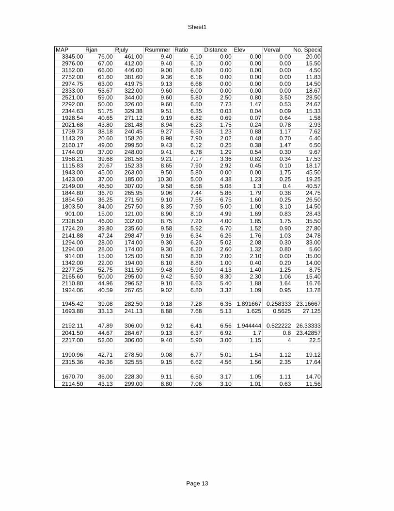
Sheet1
MAP Rjan Rjuly Rsummer Ratio Distance Elev Verval No. Specie3345.00 76.00 461.00 9.40 6.10 0.00 0.00 0.00 20.002976.00 67.00 412.00 9.40 6.10 0.00 0.00 0.00 15.503152.00 66.00 446.00 9.00 6.80 0.00 0.00 0.00 4.502752.00 61.60 381.60 9.36 6.16 0.00 0.00 0.00 11.832974.75 63.00 419.75 9.13 6.68 0.00 0.00 0.00 14.502333.00 53.67 322.00 9.60 6.00 0.00 0.00 0.00 18.672521.00 59.00 344.00 9.60 5.80 2.50 0.80 3.50 28.502292.00 50.00 326.00 9.60 6.50 7.73 1.47 0.53 24.672344.63 51.75 329.38 9.51 6.35 0.03 0.04 0.09 15.331928.54 40.65 271.12 9.19 6.82 0.69 0.07 0.64 1.582021.68 43.80 281.48 8.94 6.23 1.75 0.24 0.78 2.931739.73 38.18 240.45 9.27 6.50 1.23 0.88 1.17 7.621143.20 20.60 158.20 8.98 7.90 2.02 0.48 0.70 6.402160.17 49.00 299.50 9.43 6.12 0.25 0.38 1.47 6.501744.00 37.00 248.00 9.41 6.78 1.29 0.54 0.30 9.671958.21 39.68 281.58 9.21 7.17 3.36 0.82 0.34 17.531115.83 20.67 152.33 8.65 7.90 2.92 0.45 0.10 18.171943.00 45.00 263.00 9.50 5.80 0.00 0.00 1.75 45.501423.00 37.00 185.00 10.30 5.00 4.38 1.23 0.25 19.252149.00 46.50 307.00 9.58 6.58 5.08 1.3 0.4 40.571844.80 36.70 265.95 9.06 7.44 5.86 1.79 0.38 24.751854.50 36.25 271.50 9.10 7.55 6.75 1.60 0.25 26.501803.50 34.00 257.50 8.35 7.90 5.00 1.00 3.10 14.50901.00 15.00 121.00 8.90 8.10 4.99 1.69 0.83 28.43
2328.50 46.00 332.00 8.75 7.20 4.00 1.85 1.75 35.501724.20 39.80 235.60 9.58 5.92 6.70 1.52 0.90 27.802141.88 47.24 298.47 9.16 6.34 6.26 1.76 1.03 24.781294.00 28.00 174.00 9.30 6.20 5.02 2.08 0.30 33.001294.00 28.00 174.00 9.30 6.20 2.60 1.32 0.80 5.60914.00 15.00 125.00 8.50 8.30 2.00 2.10 0.00 35.00
1342.00 22.00 194.00 8.10 8.80 1.00 0.40 0.20 14.002277.25 52.75 311.50 9.48 5.90 4.13 1.40 1.25 8.752165.60 50.00 295.00 9.42 5.90 8.30 2.30 1.06 15.402110.80 44.96 296.52 9.10 6.63 5.40 1.88 1.64 16.761924.06 40.59 267.65 9.02 6.80 3.32 1.09 0.95 13.78
1945.42 39.08 282.50 9.18 7.28 6.35 1.891667 0.258333 23.166671693.88 33.13 241.13 8.88 7.68 5.13 1.625 0.5625 27.125
2192.11 47.89 306.00 9.12 6.41 6.56 1.944444 0.522222 26.333332041.50 44.67 284.67 9.13 6.37 6.92 1.7 0.8 23.428572217.00 52.00 306.00 9.40 5.90 3.00 1.15 4 22.5
1990.96 42.71 278.50 9.08 6.77 5.01 1.54 1.12 19.122315.36 49.36 325.55 9.15 6.62 4.56 1.56 2.35 17.64
1670.70 36.00 228.30 9.11 6.50 3.17 1.05 1.11 14.702114.50 43.13 299.00 8.80 7.06 3.10 1.01 0.63 11.56
Page 13

Sheet1
s
Page 14
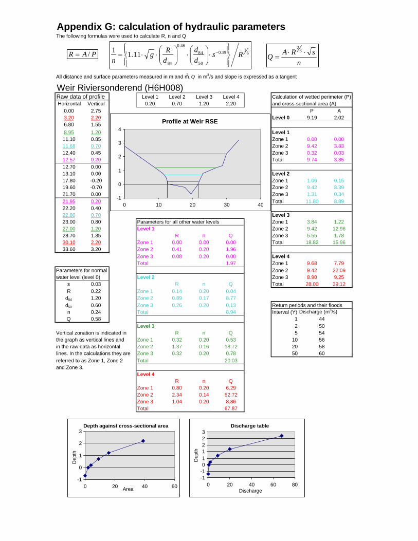
The following formulas were used to calculate R, n and Q
All distance and surface parameters measured in m and m2, Q in m3/s and slope is expressed as a tangent
Weir Riviersonderend (H6H008)Raw data of profile Level 1 Level 2 Level 3 Level 4 Calculation of wetted perimeter (P) Horizontal Vertical 0.20 0.70 1.20 2.20 and cross-sectional area (A)
0.00 2.75 P A3.20 2.20 Level 0 9.19 2.026.80 1.558.95 1.20 Level 111.10 0.85 Zone 1 0.00 0.0011.68 0.70 Zone 2 9.42 3.8312.40 0.45 Zone 3 0.32 0.0312.57 0.20 Total 9.74 3.8512.70 0.0013.10 0.00 Level 2 17.80 -0.20 Zone 1 1.06 0.1519.60 -0.70 Zone 2 9.42 8.3921.70 0.00 Zone 3 1.31 0.3421.95 0.20 Total 11.80 8.8922.20 0.4022.80 0.70 Level 3 23.00 0.80 Parameters for all other water levels Zone 1 3.84 1.2227.00 1.20 Level 1 Zone 2 9.42 12.9628.70 1.35 R n Q Zone 3 5.55 1.7830.10 2.20 Zone 1 0.00 0.00 0.00 Total 18.82 15.9633.60 3.20 Zone 2 0.41 0.20 1.96
Zone 3 0.08 0.20 0.00 Level 4 Total 1.97 Zone 1 9.68 7.79
Parameters for normal Zone 2 9.42 22.09water level (level 0) Level 2 Zone 3 8.90 9.25
s 0.03 R n Q Total 28.00 39.12R 0.22 Zone 1 0.14 0.20 0.04
d84 1.20 Zone 2 0.89 0.17 8.77d50 0.60 Zone 3 0.26 0.20 0.13 Return periods and their floodsn 0.24 Total 8.94 Interval (Y) Discharge (m3/s)Q 0.58 1 44
Level 3 2 50Vertical zonation is indicated in R n Q 5 54the graph as vertical lines and Zone 1 0.32 0.20 0.53 10 56in the raw data as horizontal Zone 2 1.37 0.16 18.72 20 58lines. In the calculations they are Zone 3 0.32 0.20 0.78 50 60referred to as Zone 1, Zone 2 Total 20.03and Zone 3.
Level 4 R n QZone 1 0.80 0.20 6.29Zone 2 2.34 0.14 52.72Zone 3 1.04 0.20 8.86Total 67.87
Appendix G: calculation of hydraulic parameters
Profile at Weir RSE
-1
0
1
2
3
4
0 10 20 30 40
Depth against cross-sectional area
-1
0
1
2
3
0 20 40 60Area
Dep
th
Discharge table
-1-1011223
0 20 40 60 80Discharge
Dep
th
PAR /= 6139.0
50
84
46.0
84
11.11 Rsdd
dRg
n ⎪⎭
⎪⎬⎫
⎪⎩
⎪⎨⎧
⋅⎟⎟⎠
⎞⎜⎜⎝
⎛⋅⎟⎟
⎠
⎞⎜⎜⎝
⎛⋅⋅= −
nsRAQ ⋅⋅
=3
2
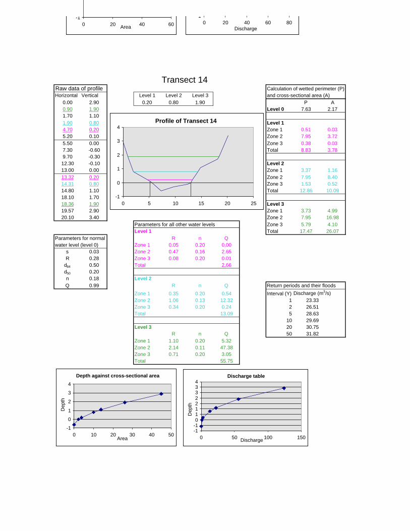
Transect 14Raw data of profile Calculation of wetted perimeter (P) Horizontal Vertical Level 1 Level 2 Level 3 and cross-sectional area (A)
0.00 2.90 0.20 0.80 1.90 P A0.90 1.90 Level 0 7.63 2.171.70 1.101.90 0.80 Level 1 4.70 0.20 Zone 1 0.51 0.035.20 0.10 Zone 2 7.95 3.725.50 0.00 Zone 3 0.38 0.037.30 -0.60 Total 8.83 3.789.70 -0.3012.30 -0.10 Level 2 13.00 0.00 Zone 1 3.37 1.1613.32 0.20 Zone 2 7.95 8.4014.31 0.80 Zone 3 1.53 0.5214.80 1.10 Total 12.86 10.0918.10 1.7018.36 1.90 Level 3 19.57 2.90 Zone 1 3.73 4.9920.10 3.40 Zone 2 7.95 16.98
Parameters for all other water levels Zone 3 5.79 4.10Level 1 Total 17.47 26.07
Parameters for normal R n Qwater level (level 0) Zone 1 0.05 0.20 0.00
s 0.03 Zone 2 0.47 0.16 2.65R 0.28 Zone 3 0.08 0.20 0.01
d84 0.50 Total 2.66d50 0.20n 0.18 Level 2Q 0.99 R n Q Return periods and their floods
Zone 1 0.35 0.20 0.54 Interval (Y) Discharge (m3/s)Zone 2 1.06 0.13 12.32 1 23.33Zone 3 0.34 0.20 0.24 2 26.51Total 13.09 5 28.63
10 29.69Level 3 20 30.75 R n Q 50 31.82Zone 1 1.10 0.20 5.32Zone 2 2.14 0.11 47.38Zone 3 0.71 0.20 3.05Total 55.75
Profile of Transect 14
-1
0
1
2
3
4
0 5 10 15 20 25
Depth against cross-sectional area
-1
0
1
2
3
4
0 10 20 30 40 50Area
Dep
th
Discharge table
-1-101122334
0 50 100 150Discharge
Dep
th
-10 20 40 60Area
10 20 40 60 80
Discharge
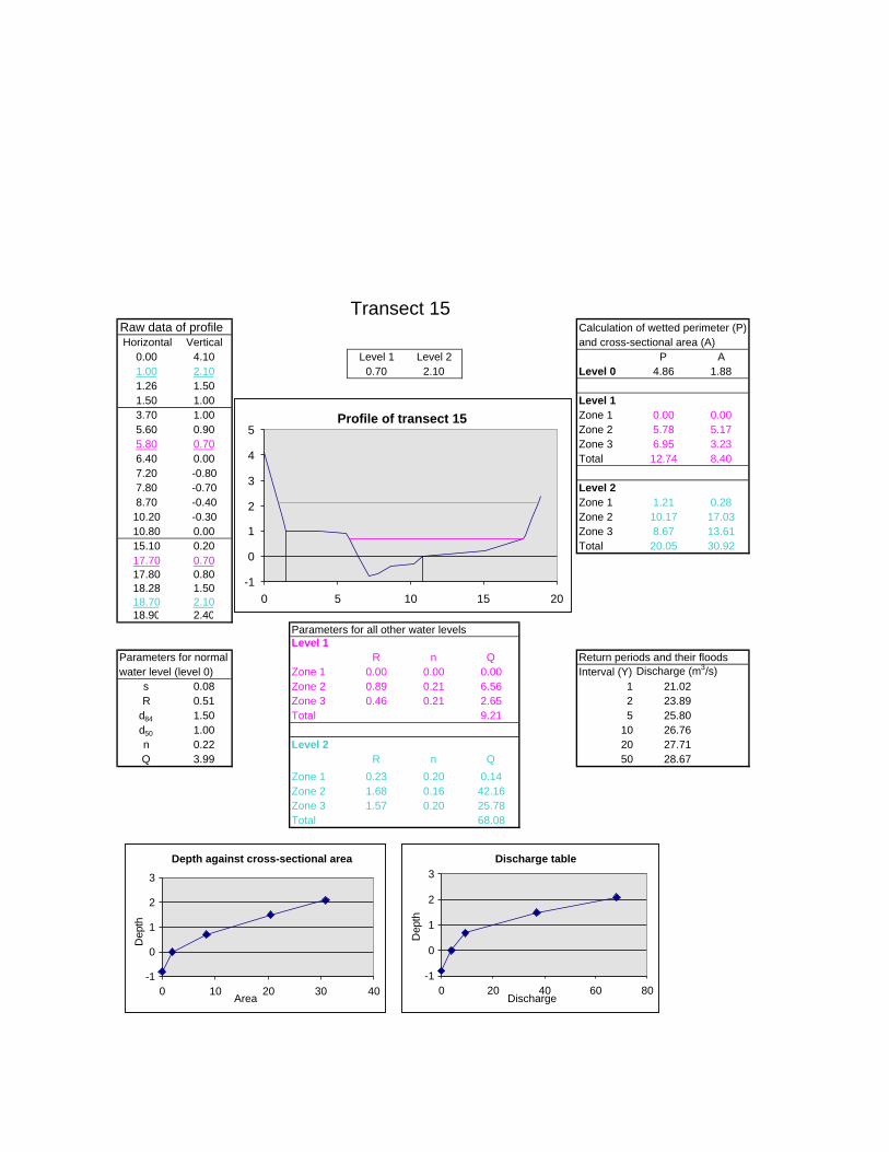
Transect 15Raw data of profile Calculation of wetted perimeter (P) Horizontal Vertical and cross-sectional area (A)
0.00 4.10 Level 1 Level 2 P A1.00 2.10 0.70 2.10 Level 0 4.86 1.881.26 1.501.50 1.00 Level 1 3.70 1.00 Zone 1 0.00 0.005.60 0.90 Zone 2 5.78 5.175.80 0.70 Zone 3 6.95 3.236.40 0.00 Total 12.74 8.407.20 -0.807.80 -0.70 Level 2 8.70 -0.40 Zone 1 1.21 0.2810.20 -0.30 Zone 2 10.17 17.0310.80 0.00 Zone 3 8.67 13.6115.10 0.20 Total 20.05 30.9217.70 0.7017.80 0.8018.28 1.5018.70 2.1018.90 2.40
Parameters for all other water levels Level 1Parameters for normal R n Q Return periods and their floodswater level (level 0) Zone 1 0.00 0.00 0.00 Interval (Y) Discharge (m3/s)
s 0.08 Zone 2 0.89 0.21 6.56 1 21.02R 0.51 Zone 3 0.46 0.21 2.65 2 23.89
d84 1.50 Total 9.21 5 25.80d50 1.00 10 26.76n 0.22 Level 2 20 27.71Q 3.99 R n Q 50 28.67
Zone 1 0.23 0.20 0.14Zone 2 1.68 0.16 42.16Zone 3 1.57 0.20 25.78Total 68.08
-0.80 0.00 0.00 0.000.00 1.88 4.40 3.990.70 8.40 11.90 9.211.50 20.51 17.02 37.122.10 30.92 17.70 68.08
Profile of transect 15
-1
0
1
2
3
4
5
0 5 10 15 20
Depth against cross-sectional area
-1
0
1
2
3
0 10 20 30 40Area
Dep
th
Discharge table
-1
0
1
2
3
0 20 40 60 80Discharge
Dep
th
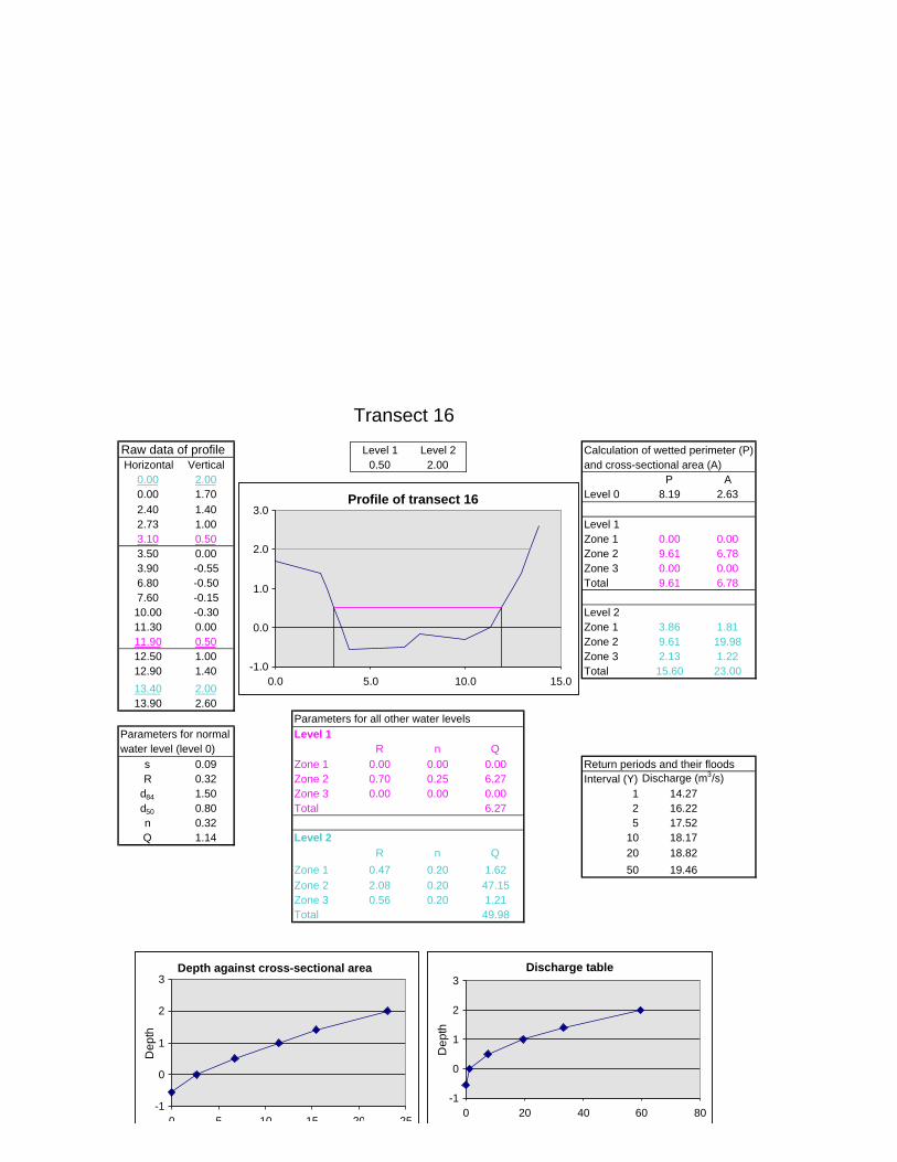
Transect 16
Raw data of profile Level 1 Level 2 Calculation of wetted perimeter (P) Horizontal Vertical 0.50 2.00 and cross-sectional area (A)
0.00 2.00 P A0.00 1.70 Level 0 8.19 2.632.40 1.402.73 1.00 Level 1 3.10 0.50 Zone 1 0.00 0.003.50 0.00 Zone 2 9.61 6.783.90 -0.55 Zone 3 0.00 0.006.80 -0.50 Total 9.61 6.787.60 -0.1510.00 -0.30 Level 2 11.30 0.00 Zone 1 3.86 1.8111.90 0.50 Zone 2 9.61 19.9812.50 1.00 Zone 3 2.13 1.2212.90 1.40 Total 15.60 23.0013.40 2.0013.90 2.60
Parameters for all other water levelsParameters for normal Level 1water level (level 0) R n Q
s 0.09 Zone 1 0.00 0.00 0.00 Return periods and their floodsR 0.32 Zone 2 0.70 0.25 6.27 Interval (Y) Discharge (m3/s)
d84 1.50 Zone 3 0.00 0.00 0.00 1 14.27d50 0.80 Total 6.27 2 16.22n 0.32 5 17.52Q 1.14 Level 2 10 18.17
R n Q 20 18.82Zone 1 0.47 0.20 1.62 50 19.46Zone 2 2.08 0.20 47.15Zone 3 0.56 0.20 1.21Total 49.98
Profile of transect 16
-1.0
0.0
1.0
2.0
3.0
0.0 5.0 10.0 15.0
Depth against cross-sectional area
-1
0
1
2
3
0 5 10 15 20 25
Dep
th
Discharge table
-1
0
1
2
3
0 20 40 60 80
Dep
th
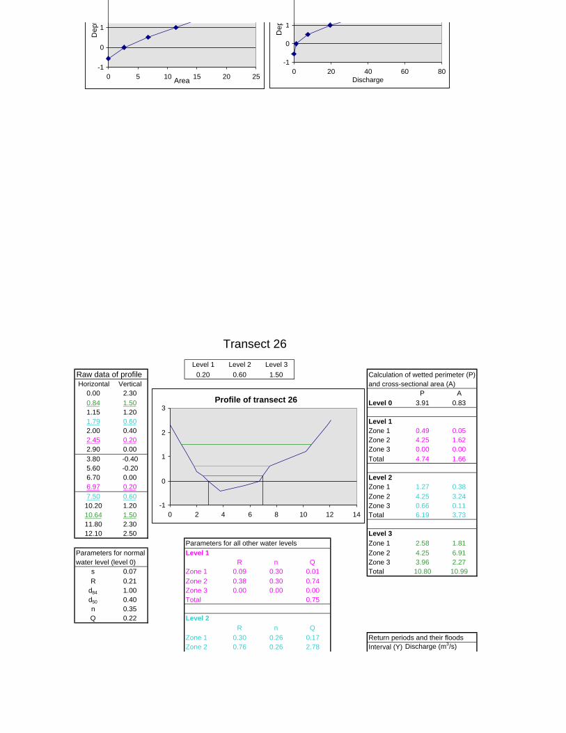
Transect 26Level 1 Level 2 Level 3
Raw data of profile 0.20 0.60 1.50 Calculation of wetted perimeter (P) Horizontal Vertical and cross-sectional area (A)
0.00 2.30 P A0.84 1.50 Level 0 3.91 0.831.15 1.20 1.79 0.60 Level 12.00 0.40 Zone 1 0.49 0.052.45 0.20 Zone 2 4.25 1.622.90 0.00 Zone 3 0.00 0.003.80 -0.40 Total 4.74 1.665.60 -0.206.70 0.00 Level 2 6.97 0.20 Zone 1 1.27 0.387.50 0.60 Zone 2 4.25 3.2410.20 1.20 Zone 3 0.66 0.1110.64 1.50 Total 6.19 3.7311.80 2.3012.10 2.50 Level 3
Parameters for all other water levels Zone 1 2.58 1.81Parameters for normal Level 1 Zone 2 4.25 6.91water level (level 0) R n Q Zone 3 3.96 2.27
s 0.07 Zone 1 0.09 0.30 0.01 Total 10.80 10.99R 0.21 Zone 2 0.38 0.30 0.74
d84 1.00 Zone 3 0.00 0.00 0.00d50 0.40 Total 0.75n 0.35Q 0.22 Level 2
R n Q Zone 1 0.30 0.26 0.17 Return periods and their floods
Zone 2 0.76 0.26 2.78 Interval (Y) Discharge (m3/s)
-1
0
1
0 5 10 15 20 25Area
Dep
t
-1
0
1
0 20 40 60 80Discharge
Dep
Profile of transect 26
-1
0
1
2
3
0 2 4 6 8 10 12 14
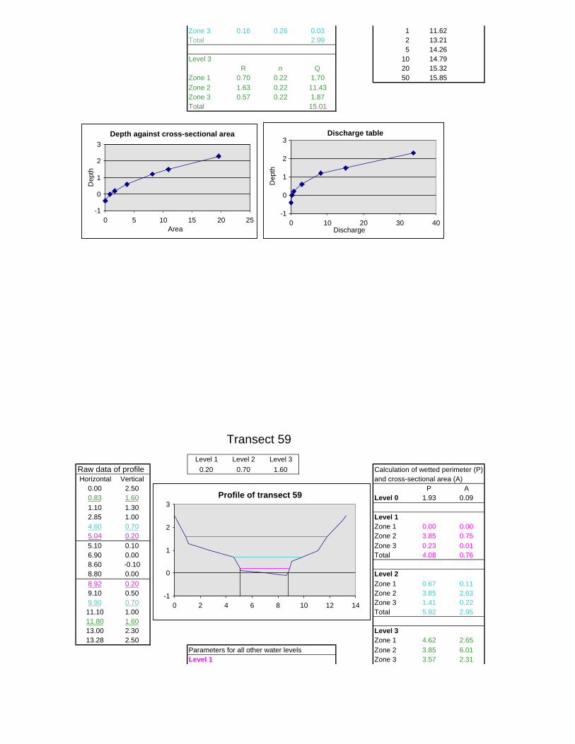
Zone 3 0.16 0.26 0.03 1 11.62Total 2.99 2 13.21
5 14.26Level 3 10 14.79 R n Q 20 15.32Zone 1 0.70 0.22 1.70 50 15.85Zone 2 1.63 0.22 11.43Zone 3 0.57 0.22 1.87Total 15.01
Transect 59Level 1 Level 2 Level 3
Raw data of profile 0.20 0.70 1.60 Calculation of wetted perimeter (P) Horizontal Vertical and cross-sectional area (A)
0.00 2.50 P A0.83 1.60 Level 0 1.93 0.091.10 1.302.85 1.00 Level 14.60 0.70 Zone 1 0.00 0.005.04 0.20 Zone 2 3.85 0.755.10 0.10 Zone 3 0.23 0.016.90 0.00 Total 4.08 0.768.60 -0.108.80 0.00 Level 28.92 0.20 Zone 1 0.67 0.119.10 0.50 Zone 2 3.85 2.639.90 0.70 Zone 3 1.41 0.2211.10 1.00 Total 5.92 2.9511.80 1.6013.00 2.30 Level 313.28 2.50 Zone 1 4.62 2.65
Parameters for all other water levels Zone 2 3.85 6.01Level 1 Zone 3 3.57 2.31
Depth against cross-sectional area
-1
0
1
2
3
0 5 10 15 20 25Area
Dep
th
Discharge table
-1
0
1
2
3
0 10 20 30 40Discharge
Dep
th
Profile of transect 59
-1
0
1
2
3
0 2 4 6 8 10 12 14
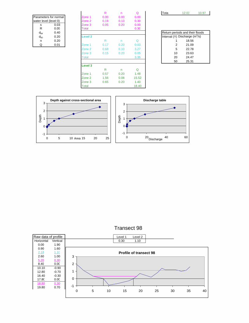
R n Q Total 12.03 10.97Parameters for normal Zone 1 0.00 0.00 0.00water level (level 0) Zone 2 0.19 0.13 0.30
s 0.03 Zone 3 0.05 0.20 0.00R 0.05 Total 0.30
d84 0.40 Return periods and their floodsd50 0.20 Level 2 Interval (Y) Discharge (m3/s)n 0.20 R n Q 1 18.56Q 0.01 Zone 1 0.17 0.20 0.03 2 21.09
Zone 2 0.68 0.10 3.27 5 22.78Zone 3 0.15 0.20 0.05 10 23.63Total 3.35 20 24.47
50 25.31Level 3 R n QZone 1 0.57 0.20 1.48Zone 2 1.56 0.08 15.52Zone 3 0.65 0.20 1.40Total 18.40
Transect 98Raw data of profile Level 1 Level 2Horizontal Vertical 0.30 1.10
0.00 1.900.90 1.602.18 1.102.60 1.005.20 0.308.40 0.0010.10 -0.9012.80 -0.7016.40 -0.3017.80 0.0018.80 0.3019.80 0.70
Profile of transect 98
-1
0
1
2
3
0 5 10 15 20 25 30 35 40
Depth against cross-sectional area
-1
0
1
2
3
0 5 10 15 20 25Area
Dep
th
Discharge table
-1
0
1
2
3
0 20 40 60Discharge
Dep
th
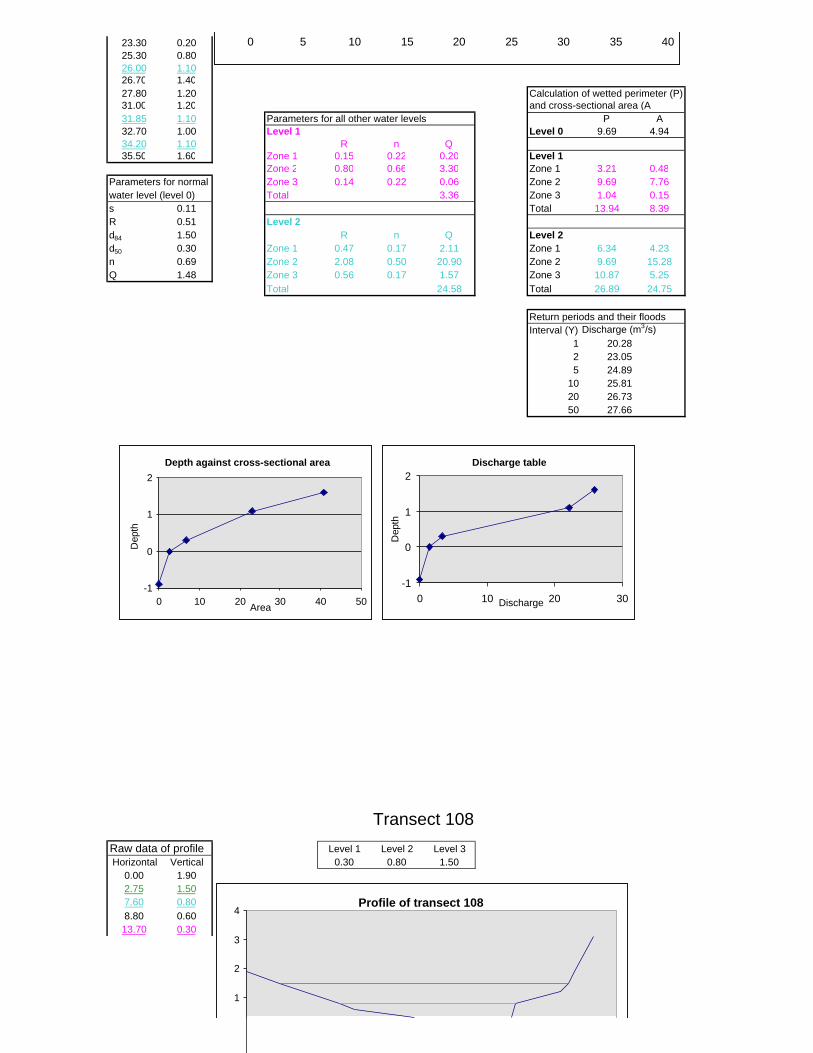
23.30 0.2025.30 0.8026.00 1.1026.70 1.4027.80 1.20 Calculation of wetted perimeter (P) 31.00 1.20 and cross-sectional area (A)31.85 1.10 Parameters for all other water levels P A32.70 1.00 Level 1 Level 0 9.69 4.9434.20 1.10 R n Q35.50 1.60 Zone 1 0.15 0.22 0.20 Level 1
Zone 2 0.80 0.66 3.30 Zone 1 3.21 0.48Parameters for normal Zone 3 0.14 0.22 0.06 Zone 2 9.69 7.76water level (level 0) Total 3.36 Zone 3 1.04 0.15s 0.11 Total 13.94 8.39R 0.51 Level 2d84 1.50 R n Q Level 2 d50 0.30 Zone 1 0.47 0.17 2.11 Zone 1 6.34 4.23n 0.69 Zone 2 2.08 0.50 20.90 Zone 2 9.69 15.28Q 1.48 Zone 3 0.56 0.17 1.57 Zone 3 10.87 5.25
Total 24.58 Total 26.89 24.75
Return periods and their floodsInterval (Y) Discharge (m3/s)
1 20.282 23.055 24.89
10 25.8120 26.7350 27.66
Transect 108Raw data of profile Level 1 Level 2 Level 3Horizontal Vertical 0.30 0.80 1.50
0.00 1.902.75 1.507.60 0.808.80 0.6013.70 0.30
0 5 10 15 20 25 30 35 40
Depth against cross-sectional area
-1
0
1
2
0 10 20 30 40 50Area
Dep
th
Discharge table
-1
0
1
2
0 10 20 30Discharge
Dep
th
Profile of transect 108
1
2
3
4
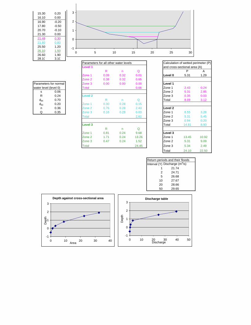
15.30 0.2016.10 0.0016.90 -0.2017.80 -0.5020.70 -0.1021.30 0.0021.48 0.3021.80 0.8025.50 1.2026.10 1.5026.60 1.9028.10 3.10
Parameters for all other water levels Calculation of wetted perimeter (P) Level 1 and cross-sectional area (A) R n Q P AZone 1 0.09 0.32 0.01 Level 0 5.31 1.29Zone 2 0.38 0.32 0.65
Parameters for normal Zone 3 0.00 0.00 0.00 Level 1 water level (level 0) Total 0.66 Zone 1 2.43 0.24
s 0.06 Zone 2 5.31 2.85R 0.24 Level 2 Zone 3 0.35 0.03
d84 0.70 R n Q Total 8.09 3.12d50 0.20 Zone 1 0.30 0.28 0.15n 0.36 Zone 2 0.76 0.28 2.43 Level 2 Q 0.35 Zone 3 0.16 0.28 0.03 Zone 1 8.55 3.28
Total 2.61 Zone 2 5.31 5.45Zone 3 0.94 0.20
Level 3 Total 14.81 8.93 R n QZone 1 0.81 0.24 9.68 Level 3 Zone 2 1.71 0.24 13.26 Zone 1 13.45 10.92Zone 3 0.47 0.24 1.52 Zone 2 5.31 9.09Total 24.45 Zone 3 5.34 2.49
Total 24.10 22.50
Return periods and their floodsInterval (Y) Discharge (m3/s)
1 21.742 24.715 26.68
10 27.6720 28.6650 29.65
-1
0
1
2
3
0 5 10 15 20 25 30
Depth against cross-sectional area
-1
0
1
2
3
0 10 20 30 40Area
Dep
th
Discharge table
-1
0
1
2
3
0 10 20 30 40 50Discharge
Dep
th
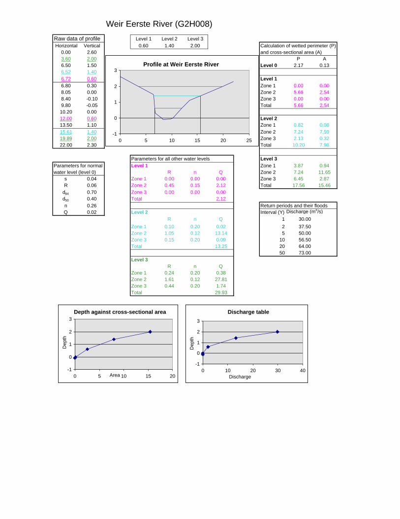
Weir Eerste River (G2H008)Raw data of profile Level 1 Level 2 Level 3Horizontal Vertical 0.60 1.40 2.00 Calculation of wetted perimeter (P)
0.00 2.60 and cross-sectional area (A)3.60 2.00 P A6.50 1.50 Level 0 2.17 0.136.52 1.406.72 0.60 Level 1 6.80 0.30 Zone 1 0.00 0.008.05 0.00 Zone 2 5.66 2.548.40 -0.10 Zone 3 0.00 0.009.80 -0.05 Total 5.66 2.5410.20 0.0012.00 0.60 Level 2 13.50 1.10 Zone 1 0.82 0.0815.61 1.40 Zone 2 7.24 7.5919.89 2.00 Zone 3 2.13 0.3222.00 2.30 Total 10.20 7.98
Parameters for all other water levels Level 3 Parameters for normal Level 1 Zone 1 3.87 0.94water level (level 0) R n Q Zone 2 7.24 11.65
s 0.04 Zone 1 0.00 0.00 0.00 Zone 3 6.45 2.87R 0.06 Zone 2 0.45 0.15 2.12 Total 17.56 15.46
d84 0.70 Zone 3 0.00 0.00 0.00d50 0.40 Total 2.12n 0.26 Return periods and their floodsQ 0.02 Level 2 Interval (Y) Discharge (m3/s)
R n Q 1 30.00Zone 1 0.10 0.20 0.02 2 37.50Zone 2 1.05 0.12 13.14 5 50.00Zone 3 0.15 0.20 0.09 10 56.50Total 13.25 20 64.00
50 73.00Level 3 R n QZone 1 0.24 0.20 0.38Zone 2 1.61 0.12 27.81Zone 3 0.44 0.20 1.74Total 29.93
Profile at Weir Eerste River
-1
0
1
2
3
0 5 10 15 20 25
Depth against cross-sectional area
-1
0
1
2
3
0 5 10 15 20Area
Dep
th
Discharge table
-1
0
1
2
3
0 10 20 30 40Discharge
Dep
th
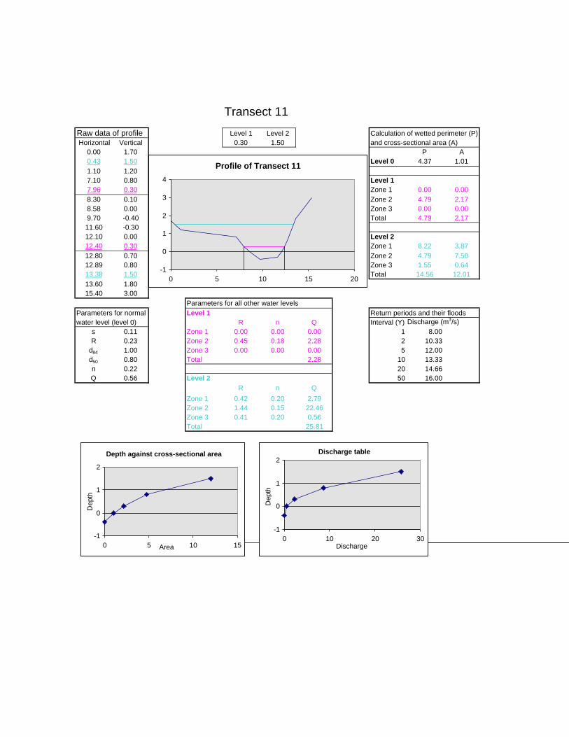
Transect 11Raw data of profile Level 1 Level 2 Calculation of wetted perimeter (P) Horizontal Vertical 0.30 1.50 and cross-sectional area (A)
0.00 1.70 P A0.43 1.50 Level 0 4.37 1.011.10 1.207.10 0.80 Level 1 7.96 0.30 Zone 1 0.00 0.008.30 0.10 Zone 2 4.79 2.178.58 0.00 Zone 3 0.00 0.009.70 -0.40 Total 4.79 2.1711.60 -0.3012.10 0.00 Level 2 12.40 0.30 Zone 1 8.22 3.8712.80 0.70 Zone 2 4.79 7.5012.89 0.80 Zone 3 1.55 0.6413.38 1.50 Total 14.56 12.0113.60 1.8015.40 3.00
Parameters for all other water levelsParameters for normal Level 1 Return periods and their floodswater level (level 0) R n Q Interval (Y) Discharge (m3/s)
s 0.11 Zone 1 0.00 0.00 0.00 1 8.00R 0.23 Zone 2 0.45 0.18 2.28 2 10.33
d84 1.00 Zone 3 0.00 0.00 0.00 5 12.00d50 0.80 Total 2.28 10 13.33n 0.22 20 14.66Q 0.56 Level 2 50 16.00
R n QZone 1 0.42 0.20 2.79Zone 2 1.44 0.15 22.46Zone 3 0.41 0.20 0.56Total 25.81
Profile of Transect 11
-1
0
1
2
3
4
0 5 10 15 20
Depth against cross-sectional area
-1
0
1
2
0 5 10 15Area
Dep
th
Discharge table
-1
0
1
2
0 10 20 30Discharge
Dep
th
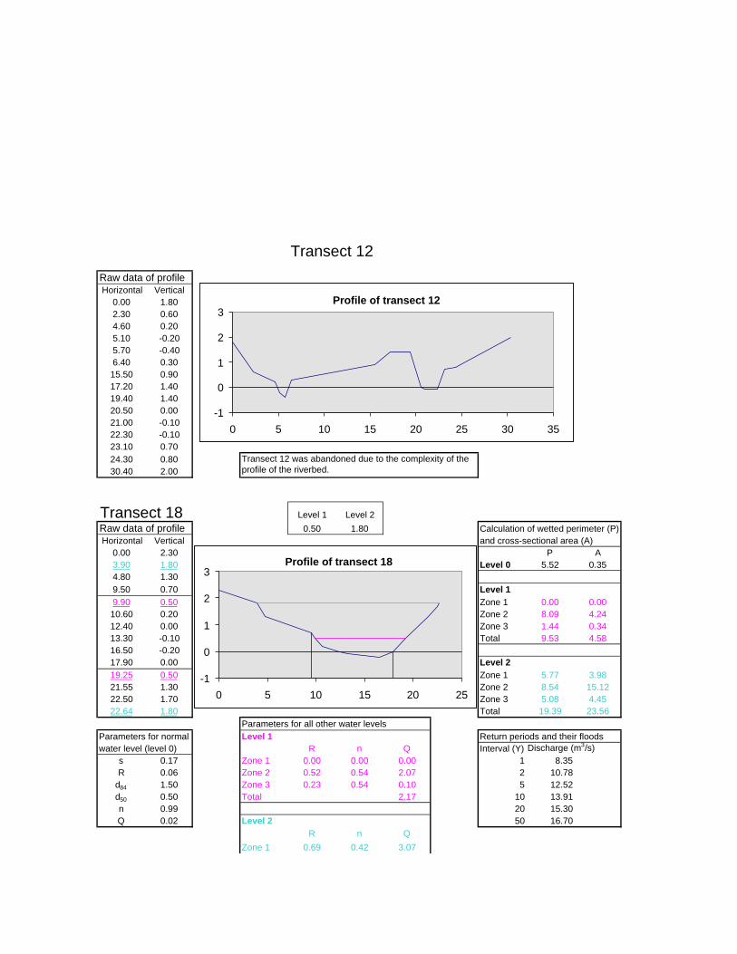
Transect 12Raw data of profileHorizontal Vertical
0.00 1.802.30 0.604.60 0.205.10 -0.205.70 -0.406.40 0.3015.50 0.9017.20 1.4019.40 1.4020.50 0.0021.00 -0.1022.30 -0.1023.10 0.7024.30 0.8030.40 2.00
Transect 18 Level 1 Level 2Raw data of profile 0.50 1.80 Calculation of wetted perimeter (P) Horizontal Vertical and cross-sectional area (A)
0.00 2.30 P A3.90 1.80 Level 0 5.52 0.354.80 1.309.50 0.70 Level 19.90 0.50 Zone 1 0.00 0.0010.60 0.20 Zone 2 8.09 4.2412.40 0.00 Zone 3 1.44 0.3413.30 -0.10 Total 9.53 4.5816.50 -0.2017.90 0.00 Level 219.25 0.50 Zone 1 5.77 3.9821.55 1.30 Zone 2 8.54 15.1222.50 1.70 Zone 3 5.08 4.4522.64 1.80 Total 19.39 23.56
Parameters for all other water levelsParameters for normal Level 1 Return periods and their floodswater level (level 0) R n Q Interval (Y) Discharge (m3/s)
s 0.17 Zone 1 0.00 0.00 0.00 1 8.35R 0.06 Zone 2 0.52 0.54 2.07 2 10.78
d84 1.50 Zone 3 0.23 0.54 0.10 5 12.52d50 0.50 Total 2.17 10 13.91n 0.99 20 15.30Q 0.02 Level 2 50 16.70
R n QZone 1 0.69 0.42 3.07
Transect 12 was abandoned due to the complexity of the profile of the riverbed.
Profile of transect 18
-1
0
1
2
3
0 5 10 15 20 25
Profile of transect 12
-1
0
1
2
3
0 5 10 15 20 25 30 35
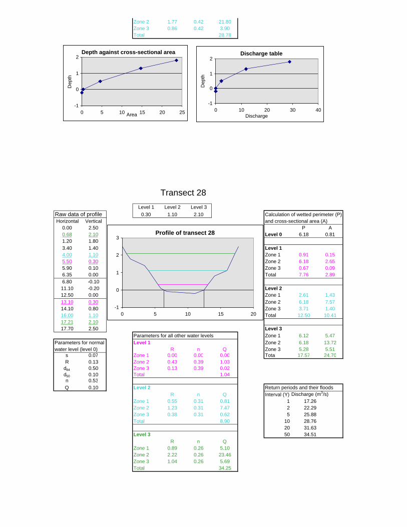
Zone 2 1.77 0.42 21.80Zone 3 0.86 0.42 3.90Total 28.78
-0.200.000.501.301.80
Transect 28Level 1 Level 2 Level 3
Raw data of profile 0.30 1.10 2.10 Calculation of wetted perimeter (P) Horizontal Vertical and cross-sectional area (A)
0.00 2.50 P A0.68 2.10 Level 0 6.18 0.811.20 1.803.40 1.40 Level 1 4.00 1.10 Zone 1 0.91 0.155.50 0.30 Zone 2 6.18 2.655.90 0.10 Zone 3 0.67 0.096.35 0.00 Total 7.76 2.896.80 -0.1011.10 -0.20 Level 2 12.50 0.00 Zone 1 2.61 1.4313.10 0.30 Zone 2 6.18 7.5714.10 0.80 Zone 3 3.71 1.4016.00 1.10 Total 12.50 10.4117.21 2.1017.70 2.50 Level 3
Parameters for all other water levels Zone 1 6.12 5.47Parameters for normal Level 1 Zone 2 6.18 13.72water level (level 0) R n Q Zone 3 5.28 5.51
s 0.07 Zone 1 0.00 0.00 0.00 Total 17.57 24.70R 0.13 Zone 2 0.43 0.39 1.03
d84 0.50 Zone 3 0.13 0.39 0.02d50 0.10 Total 1.04n 0.53Q 0.10 Level 2 Return periods and their floods
R n Q Interval (Y) Discharge (m3/s) Zone 1 0.55 0.31 0.81 1 17.26
Zone 2 1.23 0.31 7.47 2 22.29Zone 3 0.38 0.31 0.62 5 25.88Total 8.90 10 28.76
20 31.63Level 3 50 34.51 R n QZone 1 0.89 0.26 5.10Zone 2 2.22 0.26 23.46Zone 3 1.04 0.26 5.69Total 34.25
Depth against cross-sectional area
-1
0
1
2
0 5 10 15 20 25Area
Dep
th
Discharge table
-1
0
1
2
0 10 20 30 40Discharge
Dep
th
Profile of transect 28
-1
0
1
2
3
0 5 10 15 20
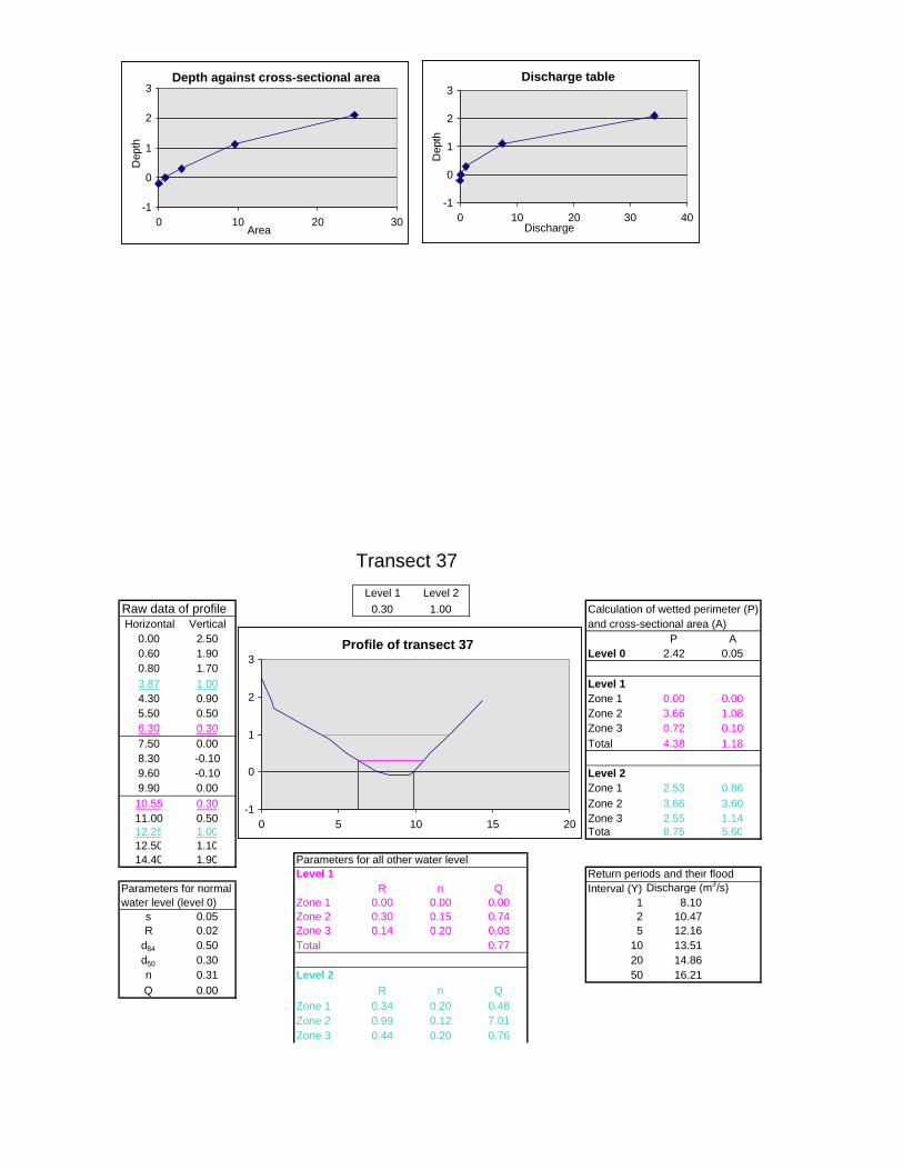
Transect 37 Level 1 Level 2
Raw data of profile 0.30 1.00 Calculation of wetted perimeter (P) Horizontal Vertical and cross-sectional area (A)
0.00 2.50 P A0.60 1.90 Level 0 2.42 0.050.80 1.703.87 1.00 Level 1 4.30 0.90 Zone 1 0.00 0.005.50 0.50 Zone 2 3.66 1.086.30 0.30 Zone 3 0.72 0.107.50 0.00 Total 4.38 1.188.30 -0.109.60 -0.10 Level 2 9.90 0.00 Zone 1 2.53 0.8610.55 0.30 Zone 2 3.66 3.6011.00 0.50 Zone 3 2.55 1.1412.25 1.00 Total 8.75 5.6012.50 1.1014.40 1.90 Parameters for all other water levels
Level 1 Return periods and their floodsParameters for normal R n Q Interval (Y) Discharge (m3/s)water level (level 0) Zone 1 0.00 0.00 0.00 1 8.10
s 0.05 Zone 2 0.30 0.15 0.74 2 10.47R 0.02 Zone 3 0.14 0.20 0.03 5 12.16
d84 0.50 Total 0.77 10 13.51d50 0.30 20 14.86n 0.31 Level 2 50 16.21Q 0.00 R n Q
Zone 1 0.34 0.20 0.48 Zone 2 0.99 0.12 7.01
Zone 3 0.44 0.20 0.76
Profile of transect 37
-1
0
1
2
3
0 5 10 15 20
Depth against cross-sectional area
-1
0
1
2
3
0 10 20 30Area
Dep
th
Discharge table
-1
0
1
2
3
0 10 20 30 40Discharge
Dep
th
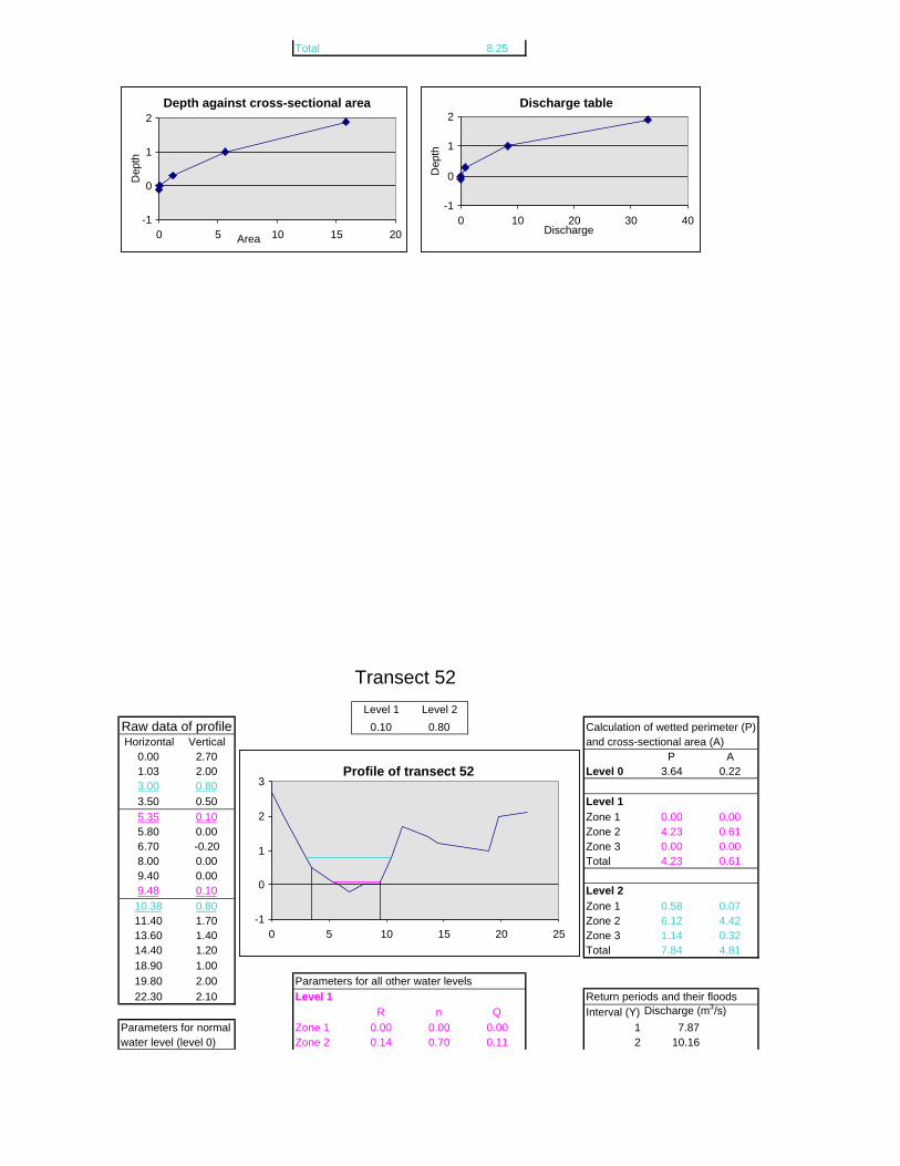
Total 8.25
Transect 52Level 1 Level 2
Raw data of profile 0.10 0.80 Calculation of wetted perimeter (P) Horizontal Vertical and cross-sectional area (A)
0.00 2.70 P A1.03 2.00 Level 0 3.64 0.223.00 0.803.50 0.50 Level 1 5.35 0.10 Zone 1 0.00 0.005.80 0.00 Zone 2 4.23 0.616.70 -0.20 Zone 3 0.00 0.008.00 0.00 Total 4.23 0.619.40 0.009.48 0.10 Level 2 10.38 0.80 Zone 1 0.58 0.0711.40 1.70 Zone 2 6.12 4.4213.60 1.40 Zone 3 1.14 0.3214.40 1.20 Total 7.84 4.8118.90 1.0019.80 2.00 Parameters for all other water levels22.30 2.10 Level 1 Return periods and their floods
R n Q Interval (Y) Discharge (m3/s)Parameters for normal Zone 1 0.00 0.00 0.00 1 7.87water level (level 0) Zone 2 0.14 0.70 0.11 2 10.16
Profile of transect 52
-1
0
1
2
3
0 5 10 15 20 25
Depth against cross-sectional area
-1
0
1
2
0 5 10 15 20Area
Dep
th
Discharge table
-1
0
1
2
0 10 20 30 40Discharge
Dep
th
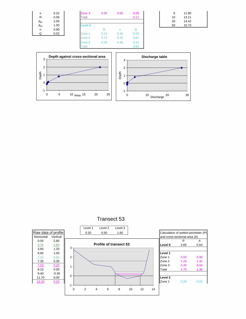
s 0.22 Zone 3 0.00 0.00 0.00 5 11.80R 0.06 Total 0.11 10 13.11
d84 2.00 20 14.42d50 1.00 Level 2 50 15.73n 0.90 R n QQ 0.02 Zone 1 0.13 0.46 0.02
Zone 2 0.72 0.46 3.67Zone 3 0.28 0.46 0.14Total 3.82
Transect 53Level 1 Level 2 Level 3
Raw data of profile 0.20 0.50 1.60 Calculation of wetted perimeter (P) Horizontal Vertical and cross-sectional area (A)
0.00 2.80 P A2.70 1.60 Level 0 3.65 0.543.60 1.206.60 1.00 Level 1 7.10 0.50 Zone 1 0.00 0.007.30 0.30 Zone 2 4.26 1.327.53 0.20 Zone 3 0.45 0.048.10 0.00 Total 4.70 1.369.40 -0.3011.70 0.00 Level 2 12.10 0.20 Zone 1 0.28 0.02
Profile of transect 53
-1
0
1
2
3
0 2 4 6 8 10 12 14
Depth against cross-sectional area
-1
0
1
2
3
0 5 10 15 20 25Area
Dep
th
Discharge table
-1
0
1
2
3
0 10 20 30Discharge
Dep
th
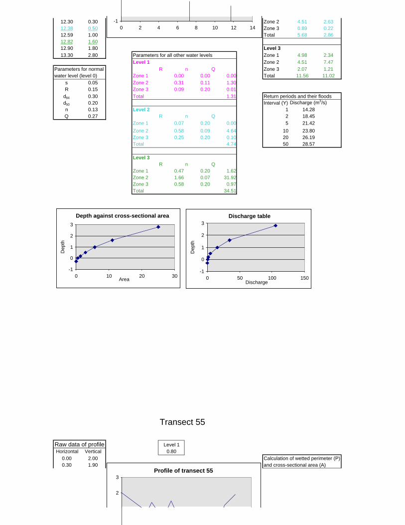
12.30 0.30 Zone 2 4.51 2.6312.38 0.50 Zone 3 0.89 0.2212.59 1.00 Total 5.68 2.8612.82 1.6012.90 1.80 Level 3 13.30 2.80 Parameters for all other water levels Zone 1 4.98 2.34
Level 1 Zone 2 4.51 7.47Parameters for normal R n Q Zone 3 2.07 1.21water level (level 0) Zone 1 0.00 0.00 0.00 Total 11.56 11.02
s 0.05 Zone 2 0.31 0.11 1.30R 0.15 Zone 3 0.09 0.20 0.01
d84 0.30 Total 1.31 Return periods and their floodsd50 0.20 Interval (Y) Discharge (m3/s)n 0.13 Level 2 1 14.28Q 0.27 R n Q 2 18.45
Zone 1 0.07 0.20 0.00 5 21.42Zone 2 0.58 0.09 4.64 10 23.80Zone 3 0.25 0.20 0.10 20 26.19Total 4.74 50 28.57
Level 3 R n QZone 1 0.47 0.20 1.62Zone 2 1.66 0.07 31.92Zone 3 0.58 0.20 0.97Total 34.51
Transect 55
Raw data of profile Level 1Horizontal Vertical 0.80
0.00 2.00 Calculation of wetted perimeter (P) 0.30 1.90 and cross-sectional area (A)
Profile of transect 55
2
3
-10 2 4 6 8 10 12 14
Depth against cross-sectional area
-1
0
1
2
3
0 10 20 30Area
Dep
th
Discharge table
-1
0
1
2
3
0 50 100 150Discharge
Dep
th
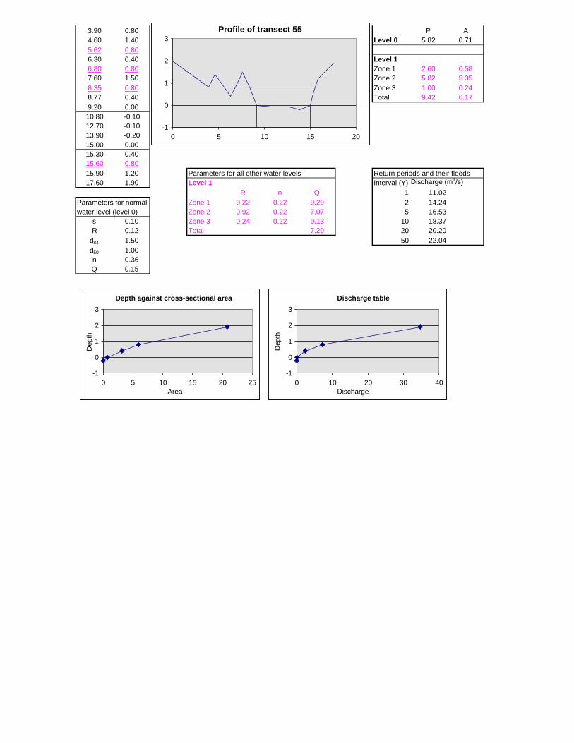
3.90 0.80 P A4.60 1.40 Level 0 5.82 0.715.62 0.806.30 0.40 Level 1 6.80 0.80 Zone 1 2.60 0.587.60 1.50 Zone 2 5.82 5.358.35 0.80 Zone 3 1.00 0.248.77 0.40 Total 9.42 6.179.20 0.0010.80 -0.1012.70 -0.1013.90 -0.2015.00 0.0015.30 0.4015.60 0.8015.90 1.20 Parameters for all other water levels Return periods and their floods17.60 1.90 Level 1 Interval (Y) Discharge (m3/s)
R n Q 1 11.02Parameters for normal Zone 1 0.22 0.22 0.29 2 14.24water level (level 0) Zone 2 0.92 0.22 7.07 5 16.53
s 0.10 Zone 3 0.24 0.22 0.13 10 18.37R 0.12 Total 7.20 20 20.20
d84 1.50 50 22.04d50 1.00n 0.36Q 0.15
Profile of transect 55
-1
0
1
2
3
0 5 10 15 20
Depth against cross-sectional area
-1
0
1
2
3
0 5 10 15 20 25Area
Dep
th
Discharge table
-1
0
1
2
3
0 10 20 30 40Discharge
Dep
th
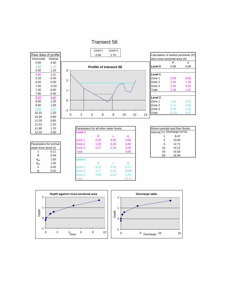
Transect 56Level 1 Level 2
Raw data of profile 0.60 1.70 Calculation of wetted perimeter (P) Horizontal Vertical and cross-sectional area (A)
0.00 2.60 P A1.60 1.70 Level 0 0.99 0.092.50 1.204.45 0.60 Level 1 5.10 0.40 Zone 1 0.00 0.006.40 0.00 Zone 2 2.99 1.357.00 -0.20 Zone 3 0.28 0.027.30 0.00 Total 3.28 1.377.80 0.408.00 0.60 Level 2 8.60 1.20 Zone 1 1.03 0.238.90 1.50 Zone 2 5.71 6.669.90 1.70 Zone 3 5.55 2.1910.15 1.20 Total 12.29 9.0710.30 0.9011.20 0.8011.53 1.2011.95 1.70 Parameters for all other water levels Return periods and their floods12.20 2.00 Level 1 Interval (Y) Discharge (m3/s)
R n Q 1 8.47Zone 1 0.00 0.00 0.00 2 10.94
Parameters for normal Zone 2 0.39 0.28 0.90 5 12.71water level (level 0) Zone 3 0.07 0.28 0.00 10 14.12
s 0.11 Total 0.90 20 15.53R 0.09 50 16.94
d84 1.50 Level 2d50 1.00 R n Qn 0.42 Zone 1 0.22 0.23 0.12Q 0.01 Zone 2 1.17 0.23 10.86
Zone 3 0.39 0.23 1.73Total 12.71
Profile of transect 56
-1
0
1
2
3
0 2 4 6 8 10 12 14
Depth against cross-sectional area
-1
0
1
2
0 2 4 6 8 10Area
Dep
th
Discharge table
-1
0
1
2
0 5 10 15Discharge
Dep
th
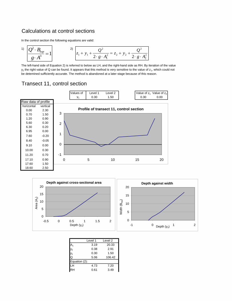
Calculations at control sectionsIn the control section the following equations are valid:
1) 2)
The left-hand side of Equation 2) is referred to below as LH, and the right-hand side as RH. By iteration of the value y2 the right value of Q can be found. It appears that this method is very sensitive to the value of z1, which could not be detemined sufficiently accurate. The method is abandoned at a later stage because of this reason.
Transect 11, control sectionValues of Level 1 Level 2 Value of z1 Value of z2
y1 0.30 1.50 0.30 0.00Raw data of profilehorizontal vertical
0.00 2.300.70 1.50 1.20 0.90 5.60 0.306.30 0.206.95 0.007.60 -0.208.40 -0.059.10 0.00
10.00 0.3011.20 0.7017.10 0.9017.60 1.5018.60 2.50
Level 1 Level 2A1 3.19 20.33y2 0.38 2.91y1 0.30 1.50Q 5.06 106.42Equation (2):LH 4.73 7.20RH 0.61 3.49
Profile of transect 11, control section
-1
0
1
2
3
0 5 10 15 20
Depth against cross-sectional area
0
5
10
15
20
-0.5 0 0.5 1 1.5 2Depth (y2)
Are
a (A
2)
Depth against width
0
5
10
15
20
-1 0 1 2Depth (y2)
Wid
th (B
top)
13
2
=⋅⋅AgBQ top
22
2
2221
2
11 22 AgQyz
AgQyz
⋅⋅++=
⋅⋅++
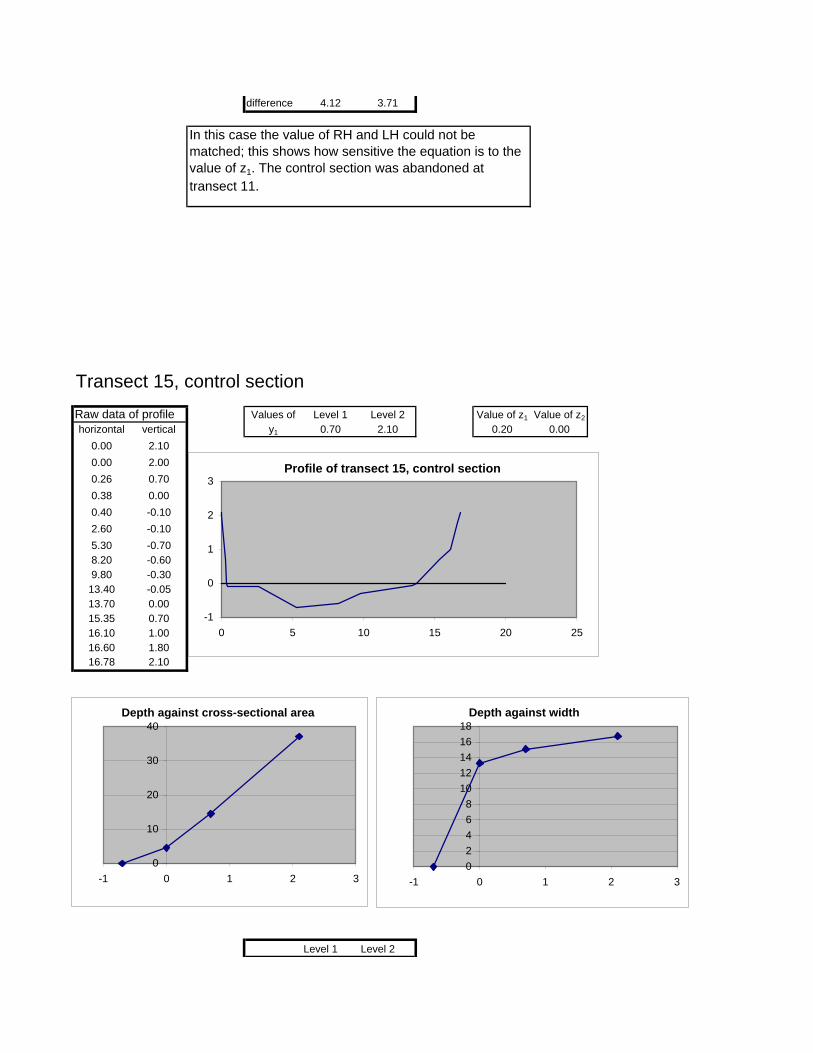
difference 4.12 3.71
Transect 15, control sectionRaw data of profile Values of Level 1 Level 2 Value of z1 Value of z2
horizontal vertical y1 0.70 2.10 0.20 0.000.00 2.100.00 2.000.26 0.700.38 0.000.40 -0.102.60 -0.105.30 -0.708.20 -0.609.80 -0.30
13.40 -0.0513.70 0.0015.35 0.7016.10 1.0016.60 1.8016.78 2.10
Level 1 Level 2
In this case the value of RH and LH could not be matched; this shows how sensitive the equation is to the value of z1. The control section was abandoned at transect 11.
Profile of transect 15, control section
-1
0
1
2
3
0 5 10 15 20 25
Depth against cross-sectional area
0
10
20
30
40
-1 0 1 2 3
Depth against width
02468
1012141618
-1 0 1 2 3
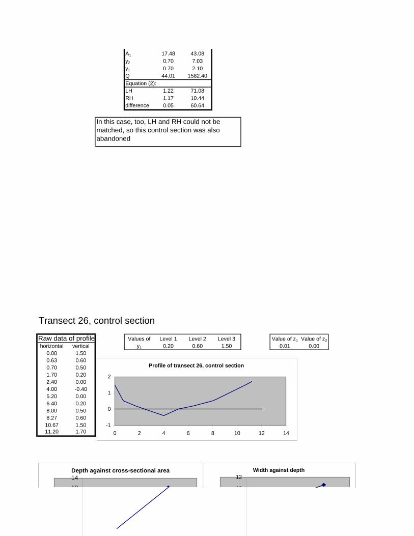
A1 17.48 43.08y2 0.70 7.03y1 0.70 2.10Q 44.01 1582.40Equation (2):LH 1.22 71.08RH 1.17 10.44difference 0.05 60.64
Transect 26, control section
Raw data of profile Values of Level 1 Level 2 Level 3 Value of z1 Value of z2
horizontal vertical y1 0.20 0.60 1.50 0.01 0.000.00 1.500.63 0.600.70 0.501.70 0.202.40 0.004.00 -0.405.20 0.006.40 0.208.00 0.508.27 0.60
10.67 1.5011.20 1.70
In this case, too, LH and RH could not be matched, so this control section was also abandoned
Profile of transect 26, control section
-1
0
1
2
0 2 4 6 8 10 12 14
Depth against cross-sectional area
1214
Width against depth
10
12
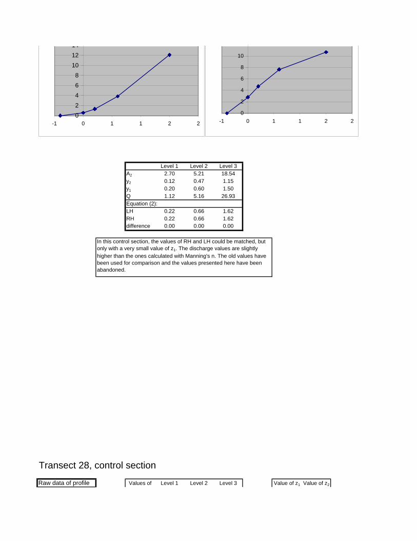
Level 1 Level 2 Level 3A2 2.70 5.21 18.54y2 0.12 0.47 1.15y1 0.20 0.60 1.50
Q 1.12 5.16 26.93 Equation (2): LH 0.22 0.66 1.62 RH 0.22 0.66 1.62 difference 0.00 0.00 0.00
Transect 28, control section
Raw data of profile Values of Level 1 Level 2 Level 3 Value of z1 Value of z2
In this control section, the values of RH and LH could be matched, but only with a very small value of z1. The discharge values are slightly higher than the ones calculated with Manning's n. The old values have been used for comparison and the values presented here have been abandoned.
02468
101214
-1 0 1 1 2 2
0
2
4
6
8
10
-1 0 1 1 2 2
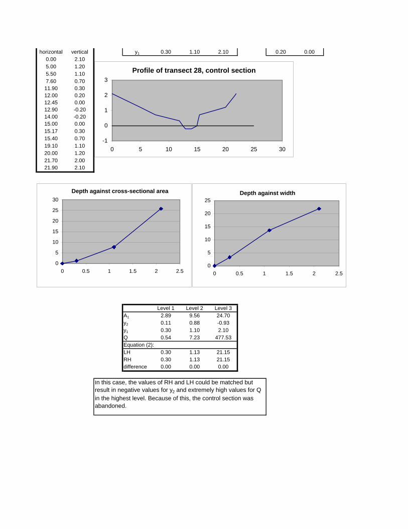
horizontal vertical y1 0.30 1.10 2.10 0.20 0.000.00 2.10 5.00 1.205.50 1.107.60 0.70
11.90 0.3012.00 0.2012.45 0.0012.90 -0.2014.00 -0.2015.00 0.0015.17 0.3015.40 0.7019.10 1.1020.00 1.2021.70 2.0021.90 2.10
Level 1 Level 2 Level 3A1 2.89 9.56 24.70y2 0.11 0.88 -0.93y1 0.30 1.10 2.10Q 0.54 7.23 477.53Equation (2):LH 0.30 1.13 21.15RH 0.30 1.13 21.15difference 0.00 0.00 0.00
In this case, the values of RH and LH could be matched but result in negative values for y2 and extremely high values for Q in the highest level. Because of this, the control section was abandoned.
Profile of transect 28, control section
-1
0
1
2
3
0 5 10 15 20 25 30
Depth against cross-sectional area
0
5
10
15
20
25
30
0 0.5 1 1.5 2 2.5
Depth against width
0
5
10
15
20
25
0 0.5 1 1.5 2 2.5