Embed Size (px)
Citation preview

Page 0 of 123
The Ribbon Microphone Multi‑Physics Educational Aid
by Marius van Wyk
Thesis presented in fulfilment of the requirements for the degree of Master of Engineering (Electronics) at the Stellenbosch University
Supervisor: Prof. Petrie Meyer
December 2017

DECLARATION
i
DECLARATION
By submitting this thesis electronically, I declare that the entirety of the work contained therein is
my own, original work, that I am the authorship owner thereof (unless to the extent explicitly
otherwise stated) and that I have not previously in its entirety or in part submitted it for obtaining
any qualification.
Date: December 2017 Su
Copyright © 2017 Stellenbosch University
All rights reserved
Stellenbosch University https://scholar.sun.ac.za
ABSTRACT
ii
ABSTRACT
Engineering education has historically been mostly mathematics based, with advanced
mathematics used to derive simple models for physics phenomena and then using these models to
study basic behaviour. However, recent years have seen a proliferation in numerical multi-physics
analysis software that performs finite element and finite volume analysis to provide high accuracy
solutions to problems. It provides visualisation of solutions that were not possible earlier, thereby
giving engineers new insight into problems and solutions. Only using analysis software can
however easily cause dissociation from real-world physics and prevent early identification of flawed
solutions. To correctly interpret simulation results it is important to first understand how the
practical model behaves.
The ribbon microphone is a real-life example that can serve as a laboratory tool for students to
make the link between theory, computer simulation and the physical world. Simulation of this
seemingly simple device is not trivial. The ribbon microphone is an all-in-one example for
simulations in acoustics, mechanics, magnetics and electromagnetics – and the interaction
between these disciplines. The value of the ribbon microphone as a teaching aid can be extended
by adding transformers and electronic amplifiers to the model. The complete model can be used to
illustrate the importance of impedance matching and noise suppression.
The thesis argues a case for the ribbon microphone as a laboratory aid in engineering education.
The case for good laboratory examples is supported by related information from engineering
education publications. The thesis is structured around a selection of experiments to illustrate how
students can learn different aspects of four physics domains through exercises concerned with the
ribbon microphone. The experiments consist of computer simulations and real-world exercises.
Theory is provided for each physics domain as an introduction to the experiments.
Stellenbosch University https://scholar.sun.ac.za

OPSOMMING
iii
OPSOMMING
Geskiedkundig was ingenieursonderrig hoofsaaklik wiskundig geskoei, met gevorderde wiskunde
wat gebruik word om eenvoudige modelle van natuurlike verskynsels af te lei en dan hierdie
modelle te gebruik om die basiese gedrag daarvan te bestudeer. Die afgelope tyd is daar egter „n
klemverskuiwing na die gebruik van numeriese veelvuldige-fisika analisesagteware wat eindige-
element en eindige-volume analise uitvoer om hoogs akkurate oplossings vir probleme te verskaf.
Dit voorsien die gebruiker met visuele terugvoer wat voorheen nie moontlik was nie. Dit gee
ingenieurs dieper insig in probleme en oplossings. Deur slegs analisesagteware te gebruik, kan die
gebruiker egter maklik van die werklikheid vervreem word en word foutiewe oplossings nie betyds
geïdentifiseer nie. Dit is belangrik om eers die gedrag van die praktiese model te verstaan voordat
gesimuleerde oplossings met die nodige insig vertolk kan word.
Die lintmikrofoon is „n praktiese voorbeeld wat studente in die laboratorium kan gebruik om die
skakel tussen teorie, rekenaarsimulasie en die fisiese wêreld duidelik te verstaan. Simulasie van
hierdie oënskynlik eenvoudige toestel is alles behalwe eenvoudig. Die lintmikrofoon is „n
samevattende voorbeeld van akoestiek, meganika, magnetika, elektromagnetika en die interaksie
tussen hierdie dissiplines. Die waarde van die lintmikrofoon as onderrigshulpmiddel kan uitgebrei
word deur „n tranformator en elektroniese versterker by die model te voeg. Die volledige model kan
aangewend word om die belangrikheid van impedansiepassing en ruisbeheer te beklemtoon.
Die tesis stel „n saak vir die lintmikrofoon as laboratoriumhulpmiddel vir ingenieursonderrig.
Publikasies oor ingenieursonderrig ondersteun die saak vir goeie hulpmiddels. Die tesis is
gestruktureer na aanleiding van „n aantal eksperimente om aan te toon hoe studente vier
verskillende fisika dissiplines kan bestudeer deur middel van die lintmikrofoon. Die eksperimente
bestaan uit rekenaarsimulasies en praktiese oefeninge. Die nodige teorie word vir elke dissipline
verskaf as inleiding tot die betrokke eksperimente.
Stellenbosch University https://scholar.sun.ac.za
ACKNOWLEDGEMENTS
iv
ACKNOWLEDGEMENTS
I would like to express my gratitude towards the following persons:
My wife Cornel and my children Marlo, Timo and Lilo for continual encouragement and prayers.
Thank you for the days and nights that you allowed me to work on my research when you rather
would have spent personal time with me.
Petrie Meyer at SUN for guidance and inspiration. It is surely uplifting and a privilege to have
someone with so much insight appreciating my efforts.
Gerhard Roux at SUN for suggesting the research topic and your enthusiasm all along the way.
Willie Perold at SUN for the use of the vapour deposition machine and Frédéric Isingizwe
Nturambirwe for helping me to operate the machine. Also for your help to get me up and running
with COMSOL®.
Johan van der Spuy at SUN for introducing me to ANSYS®.
Niël, Derrick and Chris at the CSIR “wat my gelei het om hierdie mal perd op te saal”.
Inus at the CSIR for convincing me to write my first conference paper and shedding so much light
on various aspects of life.
Alan at the CSIR for the manufacturing of the mechanical parts of the microphone.
Louisa at the CSIR for assisting me with library loans and finding valuable articles that I would
have missed otherwise.
The rest of my relatives, friends and colleagues who kept cheering me on (and checking me up)
along the road.
And most of all – my heavenly Father, Maker of the universe, for letting me discover even more
about the intricate wonders of Your creation and Your grace throughout the journey of this thesis.
Stellenbosch University https://scholar.sun.ac.za

CONTENTS
v
TABLE OF CONTENTS
Declaration 1
Abstract 2
Opsomming 3
Acknowledgements 4
Table of Contents 5
Figures 6
Tables 8
Abbreviations 9
1 INTRODUCTION 1 1.1 Content Overview 2
2 ENGINEERING EDUCATION 3 2.1 Engineering and Science 3 2.2 History of Engineering Education 3 2.3 Experimentation 5 2.4 Consequences of Inadequate Laboratories 6 2.5 Purposeful Laboratory Experiences 6 2.6 Portable Laboratory Hardware 8 2.7 A Generation with Limited Technical Childhood Exposure 9 2.8 Physics Education 10 2.9 The Ribbon Microphone as Laboratory Aid 11
3 THE MICROPHONE 12 3.1 General Information 12 3.2 The Ribbon Microphone 12
4 TECHNICAL DEVELOPMENT OF THE RIBBON MICROPHONE 14 4.1 Patents 14 4.2 Other Publications 25 4.3 Educational Benefit of Technical Histories 26
5 MODELLING AND TESTING 27 5.1 Modelling and Simulation 27 5.2 Test Equipment 30
6 ACOUSTICS 37 6.1 Theory 38 6.2 Modelling and Simulation 43 6.3 Testing 58 6.4 Conclusion 58
7 MECHANICS 59 7.1 Theory 59 7.2 Modelling and Simulation 64 7.3 Testing 70 7.4 Conclusion 72
8 MAGNETICS 73 8.1 Theory 73 8.2 Modelling and Simulation 79 8.3 Testing 81 8.4 Conclusion 84
9 ELECTROMAGNETICS 85 9.1 Theory 85 9.2 Modelling and Simulation 90 9.3 Testing 99
Stellenbosch University https://scholar.sun.ac.za

CONTENTS
vi
9.4 Conclusion 111
10 A FINAL WORD 113
11 REFERENCES 114
12 PERMISSIONS 120
FIGURES
Figure 1: RCA 44A ribbon microphone circa 1931 [24] (Silvia Classics) 13
Figure 2: Sketches of two ribbon microphone models [28] 14
Figure 3: Frequency response vs. baffle size [28] 15
Figure 4: Path length around the baffle [28] 16
Figure 5: Bostwick‟s teleconference solution [32] 18
Figure 6: Royer‟s modern version of the ribbon microphone [26] 22
Figure 7: MEMS ribbon [49] 25
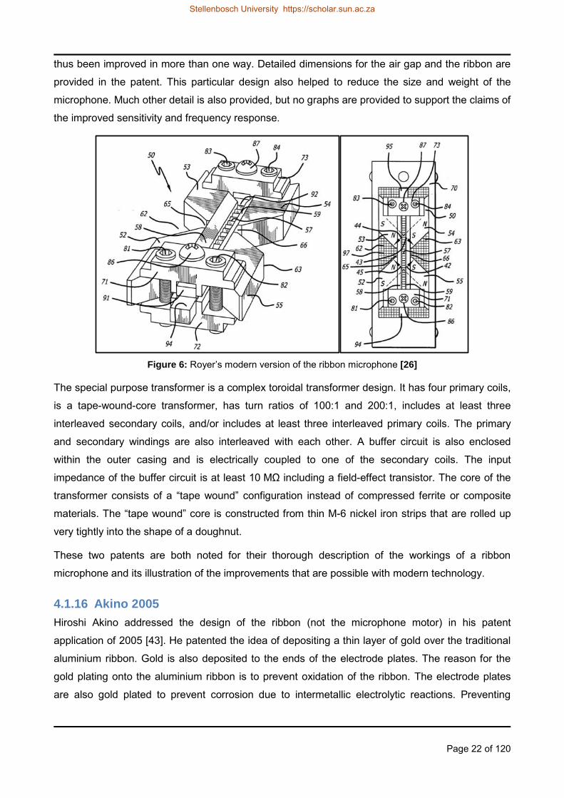
Figure 8: Marketing view of the future [52] 27
Figure 9: DIY ribbon microphone 32
Figure 10: Vapour deposition of aluminium onto PET (left), Mylar™ (centre) and Polypropylene (right) 34
Figure 11: Vapour deposition equipment setup 35
Figure 12: Transverse wave representation of a longitudinal sound wave 38
Figure 13: Relationship between particle displacement, velocity and acceleration [22] 39
Figure 14: Model of free floating disk inside a sphere (the modelling domain) 44
Figure 15: Free floating disk with narrow faces, 500 Hz - 1 kHz 45
Figure 16: Free floating disk without narrow faces, 500 Hz - 1 kHz 46
Figure 17: Free floating disk with narrow faces, 3 kHz - 4 kHz 46
Figure 18: Free floating disk without narrow faces, 3 kHz - 4 kHz 47
Figure 19: Disk resonance illustrated at 3.5 kHz (simulated with narrow faces) 47
Figure 20: Mesh illustration (grid dimensions in mm) 48
Figure 21: Free floating disk, simulated with poor mesh 48
Figure 22: Free floating disk, modelling sphere radius halved 49
Figure 23: Simulation with denser mesh (left) and less dense mesh (right) 49
Figure 24: Free floating disk with twice the weight 50
Figure 25: Free floating disk, 10 times the weight 51
Figure 26: Free floating disk twice as thick, original density 51
Figure 27: Free floating disk twice as thick, original weight 52
Figure 28: Free floating disk, less elastic 52
Figure 29: Free floating disk, more elastic 53
Figure 30: Free floating disk of double the radius, original density 54
Figure 31: Free floating disk of double the radius, original weight 54
Figure 32: Free floating disk, 2 µm aluminium, modelling sphere radius 10 mm 55
Figure 33: Free floating disk, 2 µm thin, modelling sphere radius 40 mm 55
Stellenbosch University https://scholar.sun.ac.za

CONTENTS
vii
Figure 34: Ribbon microphone in a 20 kHz sound wave [1] © 2016 IEEE 56
Figure 35: Total acoustic pressure field on the y-z plane (left) and the x-y plane (right) 57
Figure 36: Sound pressure level with 10x10 mm magnets (left) and 5x5 mm magnets (right) 57
Figure 37: Pressure gradient across the ribbon: 10x10 mm magnets (left) and 5x5 mm magnets (right) 58
Figure 38: Ribbon geometry for numeric model [65] 61
Figure 39: Spring-mass-damper model of a ribbon [65] 61
Figure 40: Numerical model of ribbon vs. experimental results [65] 63
Figure 41: Ribbon action in 300 Hz and 3 kHz sound waves 65
Figure 42: Action of ribbon with two corrugations in 300 Hz and 3 kHz sound waves 66
Figure 43: Action of ribbon with one corrugation in 300 Hz and 3 kHz sound waves 66
Figure 44: Action of ribbon with no corrugation in 300 Hz and 3 kHz sound waves 66
Figure 45: Displacement vs. frequency for ribbon with ten corrugations 68
Figure 46: Displacement vs. frequency for ribbon with zero corrugations 68
Figure 47: Velocity amplitude vs. frequency for ribbon with ten corrugations 69
Figure 48: Frequency response of corrugated ribbon (blue) and straight ribbon (red) 71
Figure 49: Stanley‟s frequency response tests for a hammered ribbon [67] 72
Figure 50: Magnetisation hysteresis loop 76
Figure 51: Magnetic field lines – perspective view and top view of slice on x-y plane 79
Figure 52: Magnetic flux density on z-x plane (left) and y-z plane (right) 79
Figure 53: Influence of pole piece design on magnetic flux density and field lines [1] © 2016 IEEE 80
Figure 54: Magnetic field strength without yoke (left) and with iron yoke (right) on the z-x plane 80
Figure 55: Magnetic field strength with mild steel yoke 81
Figure 56: Magnetic search pole 81
Figure 57: Magnetic field lines indicated by search pole 82
Figure 58: Magnetic field lines indicated by magnetic compass 82
Figure 59: SS49E field line direction 83
Figure 60: DIY Gauss meter with SS49E hall sensor 84
Figure 61: Magnetic field strength measurements outside and inside yoke 84
Figure 62: Maxwell® coil design toolkit – parameter entry 92
Figure 63: Maxwell® coil design toolkit – coil geometry 92
Figure 64: Mesh of RMX-1 model (geometry in mm) and magnetic flux density (Tesla) 93
Figure 65: Number of turns on primary winding vs. output voltage (2kΩ load) 94
Figure 66: Number of turns on primary winding vs. output voltage (3kΩ load) 94
Figure 67: Influence of source impedance on output voltage (2 kΩ load) 95
Figure 68: Influence of source impedance on output voltage (3 kΩ load) 95
Figure 69: RMX-1 results with mu-metal core and soft iron core (2 kΩ & 3 kΩ loads) 96
Figure 70: Frequency response of RMX-1 according to its competitor of the T25 97
Figure 71: Cross section of Triad SP-13 transformer 97
Figure 72: SP-48 simulation results vs. RMX-1 simulation results 98
Figure 73: RMX-1 and SP-48 transformers 99
Stellenbosch University https://scholar.sun.ac.za

CONTENTS
viii
Figure 74: Test setup for manual transformer measurements 100
Figure 75: RMX-1 simulated results (sim) vs. measured results (meas) 101
Figure 76: SP-48 simulated results (sim) vs. measured results (meas) 101
Figure 77: Test setup for automated transformer measurements 102
Figure 78: RMX-1 frequency response (automated test) 102
Figure 79: SP-48 frequency response (automated test) 103
Figure 80: AD8231 amplifier schematic 105
Figure 81: INA103 amplifier schematic 105
Figure 82: AD8231 amplifier gain test 106
Figure 83: AD8231 amplifier gain test with high pass filter 107
Figure 84: INA103 vs. AD8231 frequency response at gain of 128 107
Figure 85: Test setup with ribbon microphone and RMX-1 transformer 108
Figure 86: Ribbon microphone and SP-48 transformer 109
Figure 87: Microphone frequency response with RMX-1 (blue) and SP-48 (red) 109
Figure 88: Microphone frequency response with RMX-1 (blue) and AD8321 (green) 110
Figure 89: Microphone with AD8231 amplifier at gains of 32 and 128 110
Figure 90: Microphone with AD8231 (green) and INA103 (purple) 111
Figure 91: Ribbon microphone and AD8231 amplifier running from two AA cells 112
TABLES
Table 1: Modelling and simulation products 28
Table 2: CGS vs. SI units and its conversion factors 75
Table 3: Faraday‟s law 86
Table 4: Symbols used in Faraday‟s law 86
Table 5: RMX-1 transformer parameters 91
Table 6: SP-48 and RMX-1 transformer parameters 98
Table 7: RMX-1 measurements 100
Table 8: SP-48 measurements 100
Table 9: Impedances of secondary transformer winding at different frequencies 104
Table 10: RMX-1 power transfer (µW) to different loads 104
Table 11: SP-48 power transfer (µW) to different loads 104
Table 12: Gain multiplication factor to gain in dB 108
Stellenbosch University https://scholar.sun.ac.za
ABBREVIATIONS
ix
ABBREVIATIONS
ANSYS Registered trade mark – not an abbreviation
AC Alternating Current
ASIC Application-Specific Integrated Circuit
ACTEA Advances in Computational Tools for Engineering Applications
AWG American Wire Gauge
CAD Computer-Aided Design
CAE Computer-Aided Engineering
CFD Computational Fluid Dynamics
CGS Centimetre-Gram-Second
COMSOL Registered trade mark – not an abbreviation
CSIR Council for Scientific and Industrial Research
DC Direct Current
DIY Do-It-Yourself
ECSA Engineering Council of South Africa
emf electromotive force (measured in Volt)
ETK Electronic Transformer Kit
FEA Finite Element Analysis
FEM Finite Element Method
GPIB General Purpose Interface Bus
IC Integrated Circuit
IEEE Institute of Electrical and Electronics Engineers
JFET Junction Field Effect Transistor
MEMS Micro Electro-Mechanical Systems
MIL-SPEC Military Specification
MKSA Metre-Kilogram-Second-Ampere
PC Personal Computer
PET Polyethylene Terephthalate
RC Resistance Capacitance (filter network)
REW Room EQ Wizard
RMS Root-Mean-Square
SI Système International
SPL Sound Pressure Level
STEM Science, Technology, Engineering and Mathematics
SUN Stellenbosch University
URE Undergraduate Research Experience
US United States
USA United States of America
VA Volt-Ampere (power)
Stellenbosch University https://scholar.sun.ac.za

Page 1 of 120
1 INTRODUCTION
“I hear and I forget, I see and I remember, I do and I understand”
(Confucius)
“Tell me and I forget, teach me and I may remember, involve me and I learn.”
(Benjamin Franklin)
The more involved students become with the practical implementation of the theory that they are
taught, the more they will learn. Engineering education has historically been mostly mathematics
based, with advanced mathematics used to derive simple models for physics phenomena and then
using these models to study basic behaviour. However, recent years have seen a proliferation in
numerical multi-physics analysis software that performs finite element and finite volume analysis to
provide high accuracy solutions to problems. It provides visualisation of the solution that was not
possible earlier, thereby giving engineers new insight into problems and solutions. Only using
analysis software can however easily cause dissociation from real-world physics and prevent early
identification of flawed solutions. To correctly interpret simulation results it is important to first
understand how the practical model behaves.
The aim of this thesis is to show that one device, the ribbon microphone, can be used as a
laboratory tool for students to make the link between theory, computer simulation and the physical
world over a wide range of physics areas. This is attempted through the proposal of a number of
experiments and simulations, all centred around the ribbon microphone, which can be performed to
visualize a specific or combinations of physics areas. Four physics domains are covered in the
thesis through a selection of simulated and real-world experiments concerning the ribbon
microphone. The physics domains are:
Acoustics
Mechanics
Magnetics
Low frequency, low energy electromagnetics
The acoustics domain is addressed by a simulation experiment to illustrate how an object with
limited size and mass will behave compared to the theoretical displacement of an infinitely large
object with zero mass. The experiment is also used to illustrate the challenges of extreme ratios
and the importance of meshing during simulation.
The mechanics domain is addressed by a modelling and simulation experiment to illustrate how
different ribbon designs will influence the deflection and resonance of the ribbon in a sound wave.
Stellenbosch University https://scholar.sun.ac.za

Page 2 of 120
The experiment is concluded with an acoustic test with the ribbon microphone that validates the
simulation results, showing that a ribbon with more corrugations has a better low frequency
response.
The magnetics domain is addressed by a modelling and simulation experiment to illustrate the
direction of magnetic field lines and the magnetic field strength inside and around the microphone.
It also includes an experiment to illustrate how the magnetic field strength can be manipulated with
an iron yoke. Two real-world experiments are used to confirm the validity of the simulated results.
The electromagnetics domain is addressed by adding transformers to the microphone system and
conducting both simulation and physical experiments with the transformers to illustrate the concept
of impedance matching. To conclude the chapter an experiment with an electronic amplifier is
performed to illustrate the advantages and disadvantages of transformers vs. electronic amplifiers.
A paper based on chapters 6 to 8 of the thesis has been delivered at a conference [1] and a
follow-up paper based on chapter 9 is currently scheduled for presentation.
1.1 Content Overview
The aim of this thesis is to present a selection of experiments to illustrate how students can learn
about the aspects of four different physics domains through exercises that are concerned with the
ribbon microphone. The experiments consist of computer simulations and real-world exercises.
Theory is provided for each physics domain as an introduction to the experiments. The outline of
the thesis therefore, departs from the typical research layout. The thesis is organised by physics
topic, with each chapter showing how the ribbon microphone can be used to introduce a particular
physics topic.
Chapter one is a short introduction to the thesis.
Chapter two supports the thesis with literature about engineering education and the importance of
laboratory experiences in education.
Chapter three provides a brief history and background information on microphones in general and
an introduction to the ribbon microphone in particular.
Chapter four expands on the history of the ribbon microphone with a series of patents to illustrate
the progression of the ribbon microphone over eighty years.
Chapter five is used to describe the simulation software and hardware used in later chapters.
Chapter six to nine explores in detail the four physics domains of the ribbon microphone with
theory of the physics, software modelling and simulation, laboratory tests and conclusions.
Stellenbosch University https://scholar.sun.ac.za
Page 3 of 120
2 ENGINEERING EDUCATION
2.1 Engineering and Science
The connection between engineering, science and mathematics is described in [2].
The word engineer originates from the Latin verb ingeniare that means to design or devise.
Ingeniare originates from another word ingenium (the Latin word for engine) that means clever
invention. Engineering can therefore be summarised as the process of designing the human-made
elements of our world.
The word science originates from the Latin noun scientia that means knowledge. Science can be
seen as the study of the natural world.
While scientists are finding out how things work in the natural world around us, engineers are
conceiving ways to modify the world according to people‟s needs and wants. Engineering and
science do not work in isolation however, but complement each other. What scientists discover
about the laws of nature is used by engineers to create new inventions. In turn, the tools that
engineers design are used by scientists to make new discoveries that were not possible before.
Science is such an integral part of engineering that engineering can be seen as the process of
putting science to work.
Most systems are more than the sum of its parts. To fully understand a system it is not only
necessary to understand each part, but also to understand the interaction amongst the parts.
Engineering takes care of the finest details in addition to satisfying the bigger picture. Some
engineers will prefer to work on the detail, while others will prefer to design the larger system. It still
remains important however for engineers to be trained in grasping and appreciating the work on
both sides of the picture.
Engineers use modelling to test concepts and better understand the functioning of a process or
design. The model can take on the form of a drawing, mathematical equation, computer simulated
representation or scaled physical model. By using these models engineers can predict the
behaviour of different solutions before building it and testing it experimentally. This process of
predictive analysis is an important aspect of engineering design. The importance of mathematical
modelling and predictive analysis makes also mathematics an integral part of engineering.
The close relation between engineering, science and mathematics emphasises the importance of
science, technology, engineering and mathematics (STEM) education at all student levels.
2.2 History of Engineering Education
The history of engineering education in the USA can be found in the background information to [3].
The chronicles of graduate engineering education belongs mostly to the post-World War II era. In
Stellenbosch University https://scholar.sun.ac.za

Page 4 of 120
the USA for example, the number of graduate engineers before the war quadrupled by 1949 and
by the 1970s master‟s degrees increased 15-fold and doctoral degrees 30-fold.
The technology explosion during World War II was the first event to have a major impact on
graduate engineering education in the USA. Jet planes and atomic energy were developed during
the war and prior problems with radar were overcome. Most of the problem solvers on radar were
physicists and mathematicians. This fact and a realisation that solutions to post-war problems
would increasingly depend on scientific knowledge led to the inclusion of more science and
mathematics in the engineering curricula. Research at universities was largely supported by the
armed services. This helped to stimulate a constant supply of new graduate engineers until the
establishment of the National Science Foundation in 1950.
The academic move to include more science in the engineering curriculum was formalised in 1955
by the Report on Evaluation of Engineering Education, also known as the Grinter Report (named
after the chairman of the steering committee). The Grinter Report recommended the integrated
study of analysis, design and engineering systems to improve background knowledge of
professionals. It also included recommendations on curricular flexibility, the strengthening of
humanities and social sciences, and skills in written, graphical and verbal communication.
Furthermore, it encouraged experimental engineering. A steady increase in the number of
graduate engineering programs and graduating engineers was seen after this report. This was
good news after a decline between 1950 and 1955.
Engineering education in the USA received another incentive in 1962 with the publication of the
President's Science Advisory Committee‟s report entitled Meeting Manpower Needs in Science
and Technology. This report emphasised the urgency of graduate training (especially at doctoral
level) in engineering, sciences and mathematics in order to prevent a shortage of these skills in the
American economy. This was of course in reaction the Russian success with the Sputnik satellite.
The space-race, in part, ensured an increasing number of graduate engineers until late in the
sixties.
The engineering profession experienced a number of economic setbacks after the aerospace
cutback in 1969. By that time the swing towards science and maths was taken so far that even the
engineers who advocated it started to protest. To worsen matters, the popularity of television
around the same time caused children (potential future engineers) to stop tinkering and rather sit
glued to their television sets. The pendulum swung so far towards science that hands-on skills had
dropped tremendously by the eighties. The number of engineering graduates only started to
increase again after frustration with the lack of skills encouraged a shift back to more laboratory
time and design skills. By the nineties universities listened more to industry concerns and moved to
less science with more hands-on and applied work.
Stellenbosch University https://scholar.sun.ac.za
Page 5 of 120
In the past two decades hands-on experience was taken to a new level with the introduction of
undergraduate research experiences (UREs) by many educational institutions. Many of the
benefits of UREs are aligned with the three most important learning outcomes of the American
Association of Colleges and Universities, namely (1) intellectual and practical skills, (2) personal
and social responsibility, and (3) integrative and applied learning. Undergraduate research
encourages the experiences that transform students‟ perceptions and understanding of what they
are learning and how it is applied in real-world situations. It has personal benefits by increasing the
self-confidence and independence of students while preparing them for the next level of challenges
with an ability to tolerate obstacles. It also has professional benefits by enhancing critical thinking
and providing experiences that can be beneficial to career opportunities. UREs provide
opportunities for students to develop intellectual tools that continue building on their education by
encouraging them to ask questions as they seek to understand [4].
Modelling, aided by increasingly more powerful computers, create new possibilities to solve
problems and make discoveries that were not possible just a decade before because of the
complexities or nonlinearities of those problems. Massive system problems that could not be
solved before because of the large amounts of data to be processed are now computed daily, often
in real time. Application-specific integrated circuits (ASICs) perform computational tasks orders of
magnitude faster now than standard computer processors. The methods that are used for
laboratory experimentation are changing because data processing happens while the experiment
is run. Design and manufacturing processes are changing as more activities are automated. The
way that business is conducted is also changed by technology as the pace of electronic
communication is advancing. The advances in computer capabilities stimulated experimental
research and in some cases the ability to model natural phenomena outpaced the scientists‟
knowledge of nature itself. Increasing computer power and experimental research move in parallel,
one stimulated by the other. The technological challenge affects every field of engineering and
raises the requirements for improved education models. The accelerating pace of technological
developments is constantly posing new challenges to engineering education, even more so today
in the twenty first century. To quote Klaus Schwab, founder of the World Economic Forum: “In the
new world, it is not the big fish which eats the small fish; it‟s the fast fish which eats the slow fish.”
2.3 Experimentation
The concept that undergraduate students should be experimenters is fundamental to engineering
education. Undergraduate experimentation in the laboratory should provide students with the
fundamental tools to perform experiments as practicing engineers just as the engineering sciences
provide them with the basic tools for analysis. Like clinical training being essential to medical
practitioners, engineers should apply their knowledge of science and mathematics in an interactive
cycle of analysis, design and experimentation [5].
Stellenbosch University https://scholar.sun.ac.za
Page 6 of 120
Ferri, at al. argues that real hands-on laboratory experiences are also very effective to improve
learning and retention of knowledge [6]. The long-term memory effect of sight combined with touch
is one of the components in learning that is underestimated. Memory improves when multiple
senses (vision, touch, hearing and smell) are utilised. Each of the senses has its own processing
channel in the brain. Multi-sensory input helps to reduce the cognitive load on the brain during a
learning exercise. The tactile sensory channel for example, can transfer similar information than
the visual or the auditory channels to lighten the load on a single channel, or it can transfer
different but complementary information to construct more complete concepts in the brain. This
may explain why concepts that are reinforced through hands-on experiments are retained much
more effectively than concepts learned through non-practical learning methods. Consciously
adding checks and balances between the different channels in the brain will further enhance
understanding and recall. Hands-on experimentation provides a way to incorporate multi-sensory
modes and it can be designed to trigger deeper mental processing by means of exploratory and
reflective activities.
2.4 Consequences of Inadequate Laboratories
The lack of proper laboratory facilities in schools makes it difficult for schools to attract good
science teachers and forces teachers to teach science based on the memorisation of facts rather
than developing a fundamental understanding of scientific principles through hands-on
experiments. This approach leads to learners losing interest in science courses. Consequently the
enrolment numbers for engineering could drop and the students that do pursue an engineering
degree start with a skills disadvantage [7].
Student opinions about the motivational factors that have an effect on higher education were
captured in a study by Savage et al. at the University of Portsmouth. All of the students that were
interviewed noted that reading from PowerPoint slides is not very motivating. The novelty of new
technology had worn off in 2011 already. All but one student was of the opinion that practical work
was one of the best ways to learn, especially when the lecturer uses examples from his own
experience, i.e. explaining the theory in context with real world examples, and discussing how the
students may use that knowledge in future when working in their field. One of the students phrased
their experience as follow: “I think I get motivated by something more if I think that it is going to be
meaningful and used in real life rather than something that is just there and you are just going to
learn it for the sake of it and you are never going to use it in real life.” [8]
2.5 Purposeful Laboratory Experiences
For undergraduates to study and experience science and engineering as if they were working
scientists and engineers, they will need access to laboratories at non-prescribed times to complete
their research projects, instead of completing it in predetermined blocks of time. When large
Stellenbosch University https://scholar.sun.ac.za
Page 7 of 120
groups of students are required to perform laboratory work in predetermined time blocks, it often
happens that the laboratory experience evolves into the rote following of prescribed activities to
arrive at some conclusion to a list of predetermined questions. There is no opportunity for
discovery and deeper analysis in this method. Students that are taught in this way and do not
progress beyond undergraduate studies, will never experience or fully appreciate how scientific
investigations are conducted or how the concepts that they study were formulated [9].
Laboratories that are designed with the primary role to reinforce lecture material, do not always
deepen the student‟s understanding of the concepts in the lecture. Traditional laboratory manuals
do not reflect the scientific process to develop hypotheses, design experiments, conduct
experiments, take into account the errors induced by the measurement equipment‟s sensitivity or
its influences on the experiment, reach conclusions, and write a report on their findings.
Curricula that include laboratory experiences that are well aligned with professional practices allow
students to develop explanations for their observations, test their explanations, then refine existing
models or build their own models through experimentation. This kind of laboratory experience is
more effective than traditional laboratories for development of student‟s abilities to design
experiments, collect and analyse data and partake in meaningful scientific communication.
With deductive experiments students first learn about a concept and then perform experiments.
With inductive experiments students first perform the experiments and then cover the applicable
material afterwards in lectures. Students initially prefer deductive experiments, but later on they
value inductive experiments more because it provides them with knowledge for deeper
understanding of the subsequent lecture material. Carefully designed inductive experiments may
also be used to uncover common misconceptions in a certain area before explaining the theory
and the reasoning behind these concepts [10].
Experimentation and purposeful laboratory experiences should be designed to promote a process
of higher order thinking to keep students engaged. There is no simple definition for higher order
thinking, but it can be clearly recognised when the following qualities are present:
Non-algorithmic, i.e. the path of thought or action is not specified in advance.
Complex, i.e. the correct path is not visible from a single angle.
Multiple solutions exist, i.e. there is more than one correct path, each with its own pro‟s and
con‟s, rather than a single unique solution.
It requires judgment and interpretation of subtle variations.
It contains the application of multiple criteria that could be in conflict with each other.
It involves a measure of uncertainty.
Stellenbosch University https://scholar.sun.ac.za
Page 8 of 120
Requires self-regulation (closing the feedback loop) in the thinking process.
Imposes meaning, i.e. finding a form of structure in seemingly disorder or chaos.
Effortful, i.e. there is a considerable amount of mental work required.
These qualities are in line with the Washington Accord exit-level-outcomes for engineers. The
Washington Accord was signed in 1989 and the Engineering Council of South Africa (ECSA)
became a signatory to the Accord in 1999. Therefore, these qualities also reflect the formal
education requirements for South African universities to be accredited by ECSA. Engineers can
earn qualifications with international recognition at accredited universities.
Experimentation and laboratory time should involve a fair amount of metacognitive behaviour, for
example checking one‟s own understanding, trying to relate new material to prior knowledge and
fundamental principles, monitoring for consistency, checking for common-sense, and making use
of alternative resources [11].
Advances in technology have opened up new opportunities to enhance the science teaching
experience. These “virtual” experiences however, can never be a substitute for direct laboratory
exercises. The “virtual” activities and the hands-on laboratory interactions offer different
experiences that should complement each other [12]. This statement is supported by evidence
from Feisel and Rosa showing the important role that hands-on experimentation has in engineering
education, and how performing computer simulation can never replace the experience gained
through real experimentation [13].
In a study by Liu it was shown that computer modelling combined with hands-on laboratory work is
more effective than any one of the two in isolation [14].
2.6 Portable Laboratory Hardware
The ratio of student numbers to the amount of laboratory equipment is usually high because of the
high cost and physical size of the hardware. As a result, students have to use this equipment in
groups and for a limited time only. Students do not get the opportunity to fully explore the
equipment or understand the experiment in depth. While many universities relied completely on
simulation-based activities and provided no hands-on laboratory teaching, one institution in
particular showed dramatic improvement in student engagement when simulation-only exercises
were replaced with laboratory kits that student could take home for further experimentation. Not
only did the students‟ interest improve dramatically, but their test scores also improved. It was
observed that many students doing the computer simulations without hands-on exercises lost
interest and submitted partially completed projects. The students with hands-on laboratory
experience on the other hand, strived to see the project through until it worked completely to their
satisfaction [15].
Stellenbosch University https://scholar.sun.ac.za

Page 9 of 120
Motivated by these studies, Taylor et al. developed a low-cost, hardware platform to improve the
teaching experience for systems engineering students. The hardware was affordable enough for
each student to loan the hardware for the duration of the course and to take it home or elsewhere
on campus for further work. This encouraged students to explore the system in their own time,
allowed them to take control of their own learning to best match their individual learning styles, and
hence to promote independent learning. Use of the hardware as an educational aid was so
successful in its purpose that the authors believed it could be used even as a marketing tool to
attract future students into the department. The hardware was originally developed for an MSc
course, but the experience was received so well by the MSc students that it was planned to extend
its usefulness into a final year undergraduate course [16].
In contrast to complex, high cost laboratory equipment, Ferri et al. invented small experimental
platforms to study the effect of hands-on laboratories on large enrolment classes. These platforms
are portable and affordable enough for students to own. This hardware opened up new possibilities
to teach students in non-traditional settings such as standard classrooms that have no laboratory
infrastructure and asynchronous distance education. The requirements for their portable laboratory
were to
• address concepts that are difficult to grasp by theory alone
• integrate with the theory that is taught in class
• require a low learning curve
• provide a skeleton for students who are new to the equipment
• necessitate students to draw relations between the theory and experiments
• include design, building, testing, troubleshooting, analysing, and exploration activities.
The study from Ferri et al. revealed that hands-on experimentation has a positive impact on both
learning and the confidence of students. They found that student performance in the laboratory
was also a good indicator of what could be expected in written tests later on. It was noticeable that
the improvements in performance and in confidence level were only seen with middle and high
achievers. The low achievers‟ test scores did not benefit from the laboratories. Unsurprisingly, their
laboratory scores were also low. This phenomenon was ascribed to the fact that the lowest
achievers skipped laboratories and only did the bare minimum to complete the measurements.
They never engaged in the higher level thinking activities [6].
2.7 A Generation with Limited Technical Childhood Exposure
Practical demonstrations are important - especially now in South Africa where many new
engineering students come from a background with limited technology exposure. They hardly ever
Stellenbosch University https://scholar.sun.ac.za

Page 10 of 120
saw their parents working with new technology or repairing anything technical. On the other hand
are students who grew up in a high-tech environment but whose only interaction with technology
remains a screen and (maybe) a keyboard. Not only in South Africa but the world over institutions
are witnessing an increasing lack of mechanics knowledge – so much that in 2006 already the
Engineering Education journal published an article on the limited mechanics knowledge of students
entering higher education in the United Kingdom [17].
2.8 Physics Education
All engineering disciplines should start with a broad selection of fundamental physics before
specialising into specific domains during later years of study. Physics is an empirical study.
Everything that we know about the principles that govern the behaviour of the physical world has
been learned through observations of events in nature. The ultimate test for theory lays in its
agreement with observations and measurements of the physical phenomena. Physics is therefore
inherently a science of measurement. Lord Kelvin (1824-1907) said that “when you can measure
what you are speaking about, and express it in numbers, you know something about it; but when
you cannot express it in numbers, your knowledge is of a meagre and unsatisfactory kind; it may
be the beginning of knowledge, but you have scarcely, in your thoughts, advanced to the stage of
science, whatever the matter may be.” [18].
Physics is introduced at school in the order of most tangible to least tangible concepts. The simpler
it is to measure something; the easier it is to explain the physics concerning it. The tuition of more
difficult concepts can build on prior knowledge of simpler concepts. It is important however, that
students understand the complexities that are added when moving to domains that are more
difficult to measure. By the time that students start with undergraduate studies they should have
been exposed at school level to a broad range of physics, but not necessarily with enough depth.
Their knowledge should include, but not be limited to, the following:
Physical and mechanical properties of matter
Motion (including conservation of momentum)
Waves (electromagnetic spectrum and sound)
Work, energy and power (including conservation of energy)
Fluid statics and fluid dynamics
Electrostatics and electrodynamics
Magnetism
Electronics
Stellenbosch University https://scholar.sun.ac.za

Page 11 of 120
Electromagnetics
Students will understand some of the physics well because of personal interaction at school with
tangible objects to test the theory. The rest however, they will only know in theory. More advanced
laboratory experiences are required during undergraduate studies to give students a better
understanding of the physics they could not test at school and, more importantly, the higher level of
physics they will be taught at undergraduate level.
2.9 The Ribbon Microphone as Laboratory Aid
Many of the physics concepts listed in 2.8 can be addressed in one way or another with the ribbon
microphone as a laboratory aid. Through simulation and/or physical experimentation it can be
applied as follow:
The construction of the ribbon can be used to demonstrate the physical and mechanical
properties of thin metal and polymer foils.
The movement of the ribbon demonstrates motion and inertia of an object in a sound wave.
Sound waves in air can be modelled with the principles of fluid dynamics.
The magnetics of the microphone is useful for many experiments with magnetism.
The electromotive force (emf) generated by the microphone is a classic example of
electrodynamics and because the emf is so small, it provides a good challenge to harness
very low levels of power and energy.
The inclusion of a transformer in the system provides a good illustration of low frequency
electromagnetics.
The inclusion of an electronic amplifier in the system provides exposure to electronics in
more than one way.
While the physics in 2.8 can be shown through numerous other examples, having one
experimental vehicle which allows experiments on acoustics, mechanics, electromagnetism and
electrical circuits and noise, is invaluable. Also, because of the extreme bandwidth (20 -
20 000 Hz) required, the large dynamic range (≈ 90 dB), and the very small signal levels
developed, the microphone can illustrate a wide range of non-ideal effects. The ribbon microphone
provides students with a simple signal source in the microwatt/nanowatt range to learn about the
challenges of small signal processing.
The ribbon microphone is practical as a laboratory aid for working both in the laboratory and away
from campus. Most of the experiments in this thesis can be conducted in a study room with only
the aid of a personal computer with sound card, a multimeter and a piece of breadboard. Only a
limited number of tests require professional test equipment in a conventional electronics laboratory.
Stellenbosch University https://scholar.sun.ac.za

Page 12 of 120
3 THE MICROPHONE
3.1 General Information
The carbon microphone was developed by Thomas Edison as early as 1877. Low-cost variations
of this type of microphone can still be found in the handsets of older telephones. After the carbon
microphone, the greatest step forward was the invention of the condenser (capacitor) microphone
by Edward Wente in 1917 [19]. Condenser microphones have no magnetics. Movement of the
diaphragm causes a change in capacitance. It was the beginning of what would become a great
instrument for many decades. The human ear can perceive a multitude of sounds, ranging in
intensity (or rather sound pressure level) from 20 µPa to more than 1 Pa and ranging in frequency
from 20 Hz up to 20 kHz. For more than a century, various inventors have attempted to design a
microphone that possesses the same characteristics as the human ear. Yet, no single microphone
exists that matches all the qualities of the human ear. Various microphones are available today,
each with advantages and limitations. They can be grouped either by their construction (dynamic,
condenser or ribbon) or by their sound pattern characteristics (unidirectional (or cardioid),
bidirectional (or figure-of-eight) or omnidirectional) or by the physics behind the design (pressure or
velocity) [20] [21] [22].
The diaphragm of a pressure microphone is exposed to sound waves on one side of the
transducer only. Its output changes in accordance to the instantaneous pressure of a sound wave.
Dynamic and condenser microphones are examples of pressure microphones. A dynamic
microphone resembles the moving coil construction of a speaker; it is only much smaller and
operates in reverse. Velocity microphones are exposed to sound waves on all sides. The
difference in sound pressure (the gradient of the sound wave) between the front and the rear of the
diaphragm causes the displacement of the diaphragm. They are also known as pressure gradient
microphones. Its electrical output changes according to the instantaneous velocity of the air
particles in the sound wave. The ribbon microphone is an example of a velocity type microphone.
3.2 The Ribbon Microphone
The ribbon microphone was patented in 1932 by Harry F. Olson [23]. It consists of an extremely
thin aluminium foil ribbon suspended in a magnetic field. Pressure gradients in the air cause the
ribbon to move. The movement of the ribbon in the magnetic field generates a small electromotive
force (emf) which can be amplified and recorded. The ribbon microphone quickly gained popularity
with audio engineers for its uniform frequency response and figure-8 directivity pattern.
Stellenbosch University https://scholar.sun.ac.za

Page 13 of 120
Figure 1: RCA 44A ribbon microphone circa 1931 [24] (Silvia Classics)
When magnetic tape became the dominant recording media, ribbon microphones became less
popular and condenser microphones took over. With recordings and sound mixing processes
making use of magnetic media there is always a slight loss of high frequencies. This problem could
be remedied by large capsule condenser microphones. These microphones have a number of
resonances in the 8 kHz to 12 kHz range that enhances the high frequencies before recording. The
capsules of condenser microphones are tensioned tightly, causing the high-frequency resonances
[25].
The aluminium foil element of the ribbon microphone is only lightly tensioned, causing resonance
at very low frequencies. When digital recording became the order of the day, ribbon microphones
made a major comeback because high-frequency transfer loss was no longer an issue. Its ability to
record fast transients accurately without adding upper-range resonances became again a very
positive attribute [25]. See [26] and [27] for more detail about the fall and the rise of the ribbon
microphone throughout history.
Stellenbosch University https://scholar.sun.ac.za

Page 14 of 120
4 TECHNICAL DEVELOPMENT OF THE RIBBON MICROPHONE
Articles about the ribbon microphone dates back as far as 1931. Most of the early publications
were authored by Harry F. Olson who patented the ribbon microphone. Few publications besides
those by Olson can be found about the ribbon microphone, but plenty of patents relating to the
ribbon microphone are freely available. A selection of those patents is discussed in the paragraphs
to follow.
4.1 Patents
4.1.1 Olson 1932
Harry Olson filed the first patent for the ribbon microphone in 1931 and the patent was awarded on
25 October 1932 with the title “Apparatus for converting sound vibrations into electrical variations”
[28]. The patent illustrations are of very sturdy mechanical designs as illustrated in Figure 2.
Figure 2: Sketches of two ribbon microphone models [28]
It describes the ribbon as a relatively small item that is supported in such a way that it resembles
the motion of a particle in free air. A device of this nature is classified as a velocity microphone.
The combination of mechanical parts surrounding the ribbon is called a baffle. The size of the
baffle around the ribbon is calculated according to the highest frequency that the microphone is
designed for. The baffle should be designed so that the path length from the front of the ribbon to
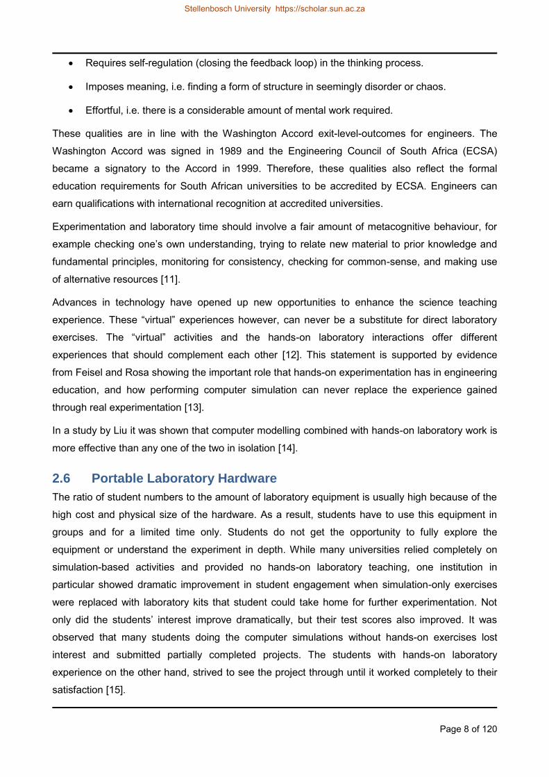
the rear of the ribbon is half the wavelength of the required frequency. Figure 3 provides a graph
from the patent to illustrate the effect of the baffle size on the frequency response of the
microphone.
Stellenbosch University https://scholar.sun.ac.za
Page 15 of 120
Figure 3: Frequency response vs. baffle size [28]
The ribbon is made of conducting material that is light in weight and that has low elasticity, for
example aluminium foil. The ribbon must not be stretched tightly between its supports. It is crimped
in order to suspend it rather loosely between its supports to promote flexibility along its whole
length. The supports are made of non-ferro-magnetic conducting material, but it is electrically
isolated from the ribbon by non-conductive material. The two signal wire leads are electrically
connected to the two ends of the ribbon. The light weight and small restoring force of the ribbon
causes its natural vibration frequency to be below the audible range. Tests that were done before
the patent submission had shown that a natural vibration frequency of approximately 10Hz
produced the most desirable results. The patent states that “When a diaphragm of small mass is
suspended in this manner its mechanical reactance is small compared to the impedance of the air.
In other words its mass reactance is negligible over a large frequency range compared to the
acoustic resistance of the air which it displaces.”
The ribbon is suspended in the air gap between two poles of a magnet in such an orientation that
its surfaces are parallel with the magnetic force lines. The magnet can be a permanent magnet or
an electromagnet. The gap between the ribbon and the magnet poles are kept to a minimum to
prevent the leakage of air around the ribbon, but the gaps must still be sufficient to prevent
frictional contact between the ribbon and the magnet. The patent suggests an air gap of 5.6mm
with the ribbon slightly narrower. The ribbon cuts the magnetic field lines while moving in the air
gap between the poles because of the sound pressure variations across it. This causes an
Stellenbosch University https://scholar.sun.ac.za

Page 16 of 120
electromotive force that is proportional to its movement. The electromotive force can be amplified
with suitable electronic equipment.
The magnetic pole pieces with its supporting structure forms the baffle. The baffle increases the
path length from the front to the back of the ribbon. The length of this path has an influence on the
response of the microphone. The paths around the top and bottom supports of the ribbon are
shorter than the paths around the baffle, but its effect is relatively small because it influences only
a small part of the ribbon. The clamping structure that secures each end of the ribbon is made of
non-magnetic material (ex. copper or brass if it is made from metal). Although it is desirable to
make the ribbon as light as possible, it is sometimes necessary to vary its thickness in order to
increase its efficiency within the particular baffle setup. The movement of the ribbon is caused by
the phase difference of the sound wave between the front and back of the ribbon. The phase
difference is determined by the distance that the sound wave has to travel around the baffle from
the front to the back of the ribbon. The greatest phase difference occurs when the path length
around the baffle is half a wavelength of the sound wave under question. Olson provides a helpful
visual representation of this effect in his patent. Figure 4 shows a horizontal cut through the
microphone and a sinusoidal representation of a sound wave. If the path length A-B around the
baffle is plotted as E-F on the axis of the sound wave, then the pressure difference between points
A and B on the ribbon will be equal to the sum of C-E plus D-F.
Figure 4: Path length around the baffle [28]
The sound intensity at the opposite sides of the baffle is virtually the same for all wavelengths that
are longer than twice the distance around the baffle. At wavelengths shorter than this, the intensity
on the approaching side of the ribbon increases and the intensity at the retreating side decreases.
The reasoning follows that the pressure difference across the ribbon is proportional to the
frequency as long as the distance around the baffle is less than half the wave length. Due to the
nature of the design the ribbon microphone exhibits very directional characteristics. Sound waves
Stellenbosch University https://scholar.sun.ac.za

Page 17 of 120
coming from an angle will produce less of a pressure difference across the ribbon. A sound wave
directly from the side will produce virtually zero pressure difference. The pressure difference can
be calculated with simple trigonometry rules.
An alternative design is also provided in the patent. The alternative design does not make use of a
ribbon, but of a lightweight diaphragm. This design is however overly complicated and will not be
discussed further.
4.1.2 Olson & Weinberger 1933
In 1933 Olson, in cooperation with Julius Weinberger, filed a patent that made use of a
combination of the pressure gradient (velocity) ribbon microphone and a pressure component
microphone to achieve unidirectional operation [29]. Unidirectional operation is desirable in order to
improve the ratio of the sound source relative to the sound reflections in the room. The patent
achieved its purpose through the use of a normal ribbon (as in the 1931 patent) assembled in
series with a modified ribbon. The modified ribbon was adapted to act as a pressure microphone
by enclosing the back of the ribbon. The normal and modified ribbons are working in phase for
sounds generated in front of the microphone, but are out of phase for sounds originating from the
rear side of the microphone. This patent illustrates the influence of the baffle in the extreme case of
making the baffle infinitely large by enclosing the rear side of the ribbon completely.
4.1.3 Anderson 1937
Leslie Anderson added electronics to Olson and Weinberger‟s unidirectional microphone to file a
patent in 1937 [30]. The electronics made it possible to adjust the phase differences between the
two ribbons, thereby making it possible to adjust the directionality of the microphone from the
mixing desk.
4.1.4 Ruttenberg 1938
In 1938 Samuel Ruttenberg filed a patent to address one of the imperfections of the ribbon
microphone [31]. When speaking close to the microphone, the low frequencies are over
emphasised because the higher frequencies are attenuated. The high frequency attenuation
happens because different sections of the ribbon move out of phase. Thus one section cancels out
the electrical current that is generated during vibration of another section. The sections move out of
phase due to the fact that the ribbon is longer than the wavelength of the higher frequency sound
waves. Ruttenberg addressed this problem by designing a special housing for the microphone
which closes up the rear of the microphone with an adjustable shutter. When closing up the rear of
the microphone, its characteristics are changed from that of a velocity microphone to that of a
pressure microphone because the sound wave does not have access to the rear of the ribbon. This
idea clearly borrows from the same principles than Olson and Weinberger‟s patent on the
Stellenbosch University https://scholar.sun.ac.za

Page 18 of 120
unidirectional microphone. The microphone‟s operation in pressure mode tends to minimise the
effect of high frequencies being attenuated. This patent clearly illustrates that tampering with the
physical surroundings of the ribbon microphone, does have a distinct influence on its operation.
4.1.5 Bostwick 1938
Telephone conferencing has been around for longer than one would expect. In 1938 Lee Bostwick
already addressed the problem of feedback between speaker and microphone during
teleconferencing. He filed a patent for a device making use of two ribbon microphones and a
loudspeaker [32]. The device is constructed with a loudspeaker facing downwards onto a deflector
underneath that reflects the sound waves in a horizontal direction toward the conference
attendees. Two ribbon microphones are fitted perpendicular on top of each other, both on top of
the loudspeaker. Because of its directionality, the ribbon microphones are insensitive to the sound
waves emanating from below it, but are sensitive to the voices of the conference attendees around
the table.
Figure 5: Bostwick‟s teleconference solution [32]
4.1.6 Olson 1940
In 1940, Harry Olson filed a patent for an improved version of the 1933 unidirectional microphone
[33]. Olson discovered that he can design a unidirectional microphone with a single ribbon instead
of the dual-ribbon method used previously. Furthermore, this microphone could be easily changed
from unidirectional to bidirectional, to non-directional operation. The method of achieving this was
to place a pipe structure (resemblance of a smoking pipe) behind a single ribbon. The pipe ends in
a labyrinth that is filled with a soft fabric acting as acoustic resistance. The pipe has shutters that
Stellenbosch University https://scholar.sun.ac.za

Page 19 of 120
can be opened or closed to achieve the desired results, i.e. shutters open allows bidirectional
operation, shutters partly closed enables unidirectional operation and shutters completely closed
constrains it to non-directional operation. This patent illustrates once again the influence of the
surroundings of the ribbon on its operation.
4.1.7 Anderson 1942
Leslie Anderson built upon Olson‟s 1933 patent by filing a patent in 1942 about the magnetic
equalization of sensitivity in a unidirectional microphone [34]. It is fundamentally an improvement
on Olson and Weinberger‟s design by adding a mechanism to adjust the magnetic fields for the two
ribbons and by changing the shape of the pole pieces in such a way that it is possible to vary the
flux density of one air gap relative to the other. This patent indicates support for Olson and
Weinberger‟s idea of modifying the baffle in order to change the operation of the microphone for a
specific purpose.
4.1.8 Rogers 1942
Ernest Rogers filed a patent in 1942 for a microphone with selective discrimination between sound
sources [35]. He claimed that the microphone can be used to determine the direction of a sound
source. The microphone receives sound waves approaching the microphone straight-on, but
attenuates sound waves approaching the microphone from an angular displaced direction. The
construction of the microphone is basically four ribbon microphones assembled in an X-pattern.
The ribbons are connected to a mixing circuit in such a way that the phase relationship between
the ribbons can be adjusted. By adjusting the phase relationship, the microphone can be tuned so
that the phases of sound waves from a certain direction cancel each other out, while the phases of
sounds waves from another direction will add to each other.
4.1.9 Olson 1946
The ribbon microphone inherently has a figure-8 directivity pattern. Olson filed a patent in 1946 to
combine two ribbon microphones in a perpendicularly fashion in order to get a microphone that has
a 360° pattern on the horizontal plane [36]. This microphone would be ideal for use in orchestras
for example, recording all the instruments around it, but attenuating sound waves reflecting from
the ceiling and from the floor. Part of the idea is borrowed from Bostwick‟s teleconferencing
microphone discussed earlier [32].
4.1.10 Anderson 1947
Anderson‟s patent application in 1947 was filed as an improvement on Olson‟s 1931 design [37].
According to Anderson, Olson‟s design displayed a considerable drop in output when the distance
around baffle approaches one fourth of the sound wave‟s wavelength. Anderson‟s design claimed
to have a more uniform response over the operating range of the microphone and also to have an
Stellenbosch University https://scholar.sun.ac.za

Page 20 of 120
enhanced high frequency response compared to the conventional design. This was accomplished
by mounting one or more semi-circular bands behind the ribbon. The bands provide cavities that
are resonant at the frequencies where the enhancements are deemed necessary.
4.1.11 Olson 1950
Olson and Preston applied for a patent in 1950 that introduced a new magnet design for the ribbon
microphone [38]. The new design brought the magnet closer to the ribbon by doing away with the
pole pieces and using a magnet structure consisting of two large magnets, one on each side of the
ribbon, with an oval hole in each magnet. The holes in the magnets are there to reduce the path
length from the front to the back of the ribbon, thereby extending its upper frequency response.
Olson‟s motivation for the design is that the efficiency of the magnetic structure increases as the
magnetic source is placed closer to the air gap because the amount of leakage flux decreases. It is
also an attempt to minimise the effect of the pole pieces on the difference in sound pressure
between the front and the back of the ribbon.
4.1.12 Anderson 1954
In 1954 Anderson filed a patent concerning the magnetic circuit of the ribbon microphone [39]. This
patent addressed the problem of the air gap between the ribbon and the magnetic structure. If the
gap is too small, the ribbon might touch the structure as it moves. If the gap is made larger, then
the sensitivity of the microphone is adversely affected. Therefore the gap must be adjusted to a
very specific distance. The patent provides no recommendations about the optimum size of the air
gap or anything about the magnetics itself. It is purely an assembly method to mount the magnetic
yoke pieces accurately and reliably in a repeatable manner.
4.1.13 Fisher 1965
Charles Fisher addressed the upper frequency limit of the ribbon microphone in his 1965 patent
[40]. The patent illustrates the design of a ribbon microphone with an exceptionally large
horseshoe magnet at the base with conical pole pieces attached to the magnet. The conical pole
pieces are constructed such that it does not only taper off to the top, but also makes the opening
for the ribbon narrower as it protrudes away from the magnet. The pole pieces and the ribbon are
thus broad at the end closest to the magnet and narrow at the end furthest from the magnet. The
front to rear path around the baffle at the furthest end is thus much shorter than that of the
conventional design. The patent claims good response and directivity up to 20 kHz, but no
frequency response graphs are provided to support the claim.
4.1.14 Royer 1999
For three and a half decades (mainly the period that the condenser microphone dominated) the US
patent office did not receive any submissions concerning the ribbon microphone. David Royer and
Stellenbosch University https://scholar.sun.ac.za

Page 21 of 120
Richard Perrotta broke the silence in 1999 with their patent to modify the original ribbon
microphone [41]. The digital conversion of sound recordings was the motivation behind their
invention. Non-ribbon microphones produce large frequency dips and phase distortions that get
falsely interpreted by the digital equipment as valid data. Ribbon microphones do not have this
problem. Royer and Perrotta deemed it necessary to modify the ribbon microphone so that it could
be used at higher volume levels. To achieve the desired effect they designed a ribbon microphone
with magnetic pole pieces which are much wider from front to back and with the ribbon positioned
not in the centre, but one quarter of the pole width from the front of the microphone. In the original
ribbon microphone the pole pieces are tapered to become narrower towards the ribbon. In Royer
and Perrotta‟s design the pole pieces are purposely not tapered. The frequency response graph in
the patent application shows a very flat response from 40 Hz up to 15 kHz. Frequencies lower than
40 Hz are attenuated by as much as 5 dB (at 20 Hz) and frequencies above 15 kHz are attenuated
by as much as 7 dB (at 19 kHz). No graph is provided to compare the volume levels of the original
(prior art) with the new design. This design increases the baffle size slightly with the increased
thickness of the magnetic poles. Olson‟s 1931 patent only shows the frequency response between
100 Hz and 7 kHz, so no direct comparison can be made between the original and the new
designs concerning the effect of the baffle size on the frequency response.
4.1.15 Royer 2004
In 2004 Royer and Perrotta filed two more patents [26] [42]. They filed two patents for the same
microphone on the same day, but each application emphasised a different aspect of their
invention; thereby slightly changing the classification of each patent. One patent emphasises an
angled magnet structure to improve the sensitivity and frequency response of the microphone.
The other patent emphasises the specially designed transformer for said microphone. The
applicants incorporated some of the principals of their previous patent, but this microphone was
designed with pole pieces that taper narrower towards the ribbon (unlike the thicker magnetic poles
of the 1999 patent). The angled magnet design effectively reduces the front-to-rear distance
around the baffle. This is in accordance with Olson‟s rule that a shorter distance around the baffle
will produce a higher frequency range. The angled magnet design aids in the sensitivity of the
microphone because it maximises the amount of magnetic flux lines running perpendicular to the
ribbon. Totally perpendicular magnets would have the highest impact on the sensitivity, but that
would increase the path length around the baffle. The patent‟s design with magnets at an angle
less than 80º, provides a good compromise between the baffle length and flux direction in order to
get good sensitivity while also improving the frequency response. Royer and Perrotta made use of
Neodymium magnets in this design. The Neodymium magnets are much more powerful than the
magnets used in previous designs. The alloy for the pole pieces in this patent is Permendur or
Hyperco 90 which has a much higher magnetic permeability than iron. The magnetic structure has
Stellenbosch University https://scholar.sun.ac.za
Page 22 of 120
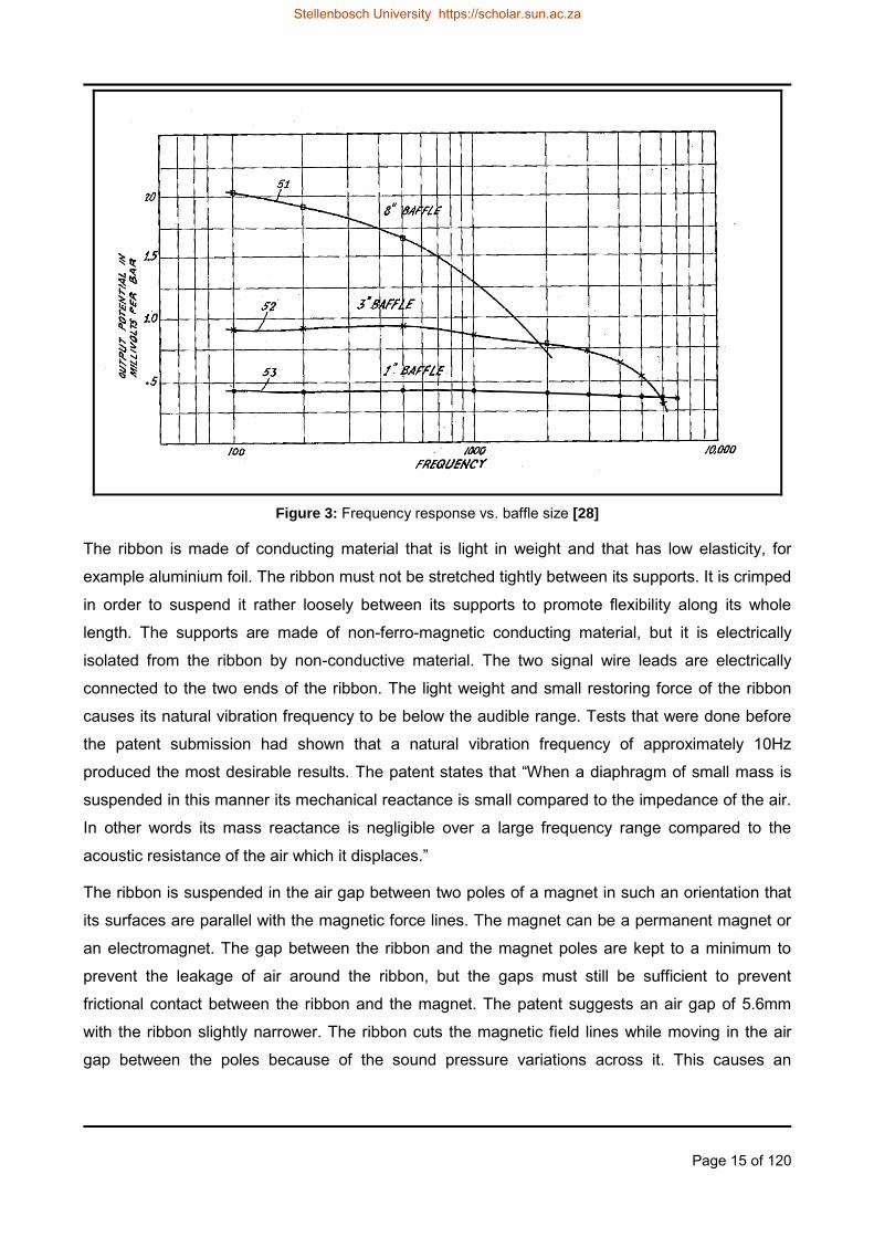
thus been improved in more than one way. Detailed dimensions for the air gap and the ribbon are
provided in the patent. This particular design also helped to reduce the size and weight of the
microphone. Much other detail is also provided, but no graphs are provided to support the claims of
the improved sensitivity and frequency response.
Figure 6: Royer‟s modern version of the ribbon microphone [26]
The special purpose transformer is a complex toroidal transformer design. It has four primary coils,
is a tape-wound-core transformer, has turn ratios of 100:1 and 200:1, includes at least three
interleaved secondary coils, and/or includes at least three interleaved primary coils. The primary
and secondary windings are also interleaved with each other. A buffer circuit is also enclosed
within the outer casing and is electrically coupled to one of the secondary coils. The input
impedance of the buffer circuit is at least 10 MΩ including a field-effect transistor. The core of the
transformer consists of a “tape wound” configuration instead of compressed ferrite or composite
materials. The “tape wound” core is constructed from thin M-6 nickel iron strips that are rolled up
very tightly into the shape of a doughnut.
These two patents are both noted for their thorough description of the workings of a ribbon
microphone and its illustration of the improvements that are possible with modern technology.
4.1.16 Akino 2005
Hiroshi Akino addressed the design of the ribbon (not the microphone motor) in his patent
application of 2005 [43]. He patented the idea of depositing a thin layer of gold over the traditional
aluminium ribbon. Gold is also deposited to the ends of the electrode plates. The reason for the
gold plating onto the aluminium ribbon is to prevent oxidation of the ribbon. The electrode plates
are also gold plated to prevent corrosion due to intermetallic electrolytic reactions. Preventing
Stellenbosch University https://scholar.sun.ac.za

Page 23 of 120
corrosion at the ribbon-electrode-junction ensures that the impedance of the junction remains as
low as possible, thereby preventing the loss in sensitivity that would usually occur over time.
4.1.17 Crowley 2005
During the same year Robert Crowley filed a lengthy patent with twenty different claims [44]. The
patent aims to enhance quality and repeatability during the manufacturing process of the ribbon
microphone. Crowley stresses the importance of the ribbon in his patent. He addresses the trade-
off between mass and resistance of the ribbon by using composite materials. The ribbon in this
patent is claimed to consist of carbon fibre nanotube filaments attached to a layer of conductive
material.
4.1.18 Tripp 2007
With the main focus still on the ribbon, Tripp and Crowley filed a patent in 2007 for the invention of
a polymer ribbon [45]. Their patent makes us of a polymer ribbon that exhibits high toughness, high
conductivity and good shape-memory. The ribbon‟s corrugated structure is formed by compressing
the ribbon between two dies and then heating and cooling it to set it permanently into this shape.
The polymer ribbon is coated with a conductive coating. The polyethylene terephthalate (PET) that
it consists of does not become brittle with age because it contains no plasticisers. The invention
claims that the ribbon will not be damaged by phantom power (48VDC applied by mixing boards)
because the PET that is used is about eight times stronger than a normal aluminium ribbon.
Another advantage of the high strength of the PET is the fact that the ribbon can be made much
thinner and thus lighter, making it more responsive to low intensity sound waves.
4.1.19 Akino 2009
In 2009 Akino patented another ribbon design [46]. In any ribbon microphone design the ribbon
must be set to a resonance frequency that is below the lowest frequency to be recorded. To
achieve this, the tension on the ribbon must be very low. The corrugated form of the ribbon helps
to realise this low tension. The corrugated ribbon is manufactured by feeding the ribbon through a
set of spur gears. According to the patent the flat areas between the corrugations cause a high
mechanical resonance within the required frequency range to be recorded. To solve this problem a
ribbon was invented onto which a special pattern is transferred by means of a roller with a transfer
mould. The selective embossing of the ribbon produces a more rigid ribbon that suppresses the
sharp resonances. On the frequency response graphs in the patent it can be seen that the
specially formed ribbon suffers less from high frequency resonances (noticeably in the region
above 10 kHz), but it suffers from lower sensitivity above 5kHz.
Stellenbosch University https://scholar.sun.ac.za

Page 24 of 120
4.1.20 Horng 2009
The National Chung-Hsing University in Taiwan recognised an opportunity to address the design of
the ribbon with the aid of micro electro-mechanical systems (MEMS) technology [47]. The patent
claims that the frequency response of the microphone will be better if its sensitivity is improved and
that the sensitivity can be improved by using a lighter ribbon. The weight and the size of the ribbon
are however restricted by conventional manufacturing processes. According to this patent it is the
size and weight restrictions of the ribbon that causes the attenuation of low and high frequencies.
By applying the techniques that are used in semiconductor fabrication and in MEMS, the patent
describes the manufacturing of a smaller diaphragm and voice coil. No dimensions are provided in
the patent to judge the reduction in size and no frequency response characteristics are given to
illustrate any improvements.
4.1.21 Cloud 2010
With new designs for the ribbon itself being thoroughly covered since 2005, Cloud and Sank‟s
patent focussed on other aspects of the ribbon microphone, namely the magnet motor assembly, a
back-wave chamber and electronics [27]. The patent introduces round magnet poles to the design.
The rounded poles cause sound waves to reflect of it in a diverging pattern, thereby diffusing the
reflected sound waves. Therefore the ribbon reacts to the sound with minimal interference from
sound waves reflecting off the pole pieces. The result is a flatter frequency response compared to
conventional flat magnets. No frequency response graphs are provided in the patent to support this
claim. Another part of the patent illustrates a different design with a horizontal ribbon and a blast
filter in front of the ribbon to protect it against high pressure sound waves. The same configuration
also has a chamber at the back of the ribbon which prevents reflected sounds from entering the
microphone from the rear. This design is completely different form the normal upright configuration
of the ribbon microphone, looking more like the ice-cream cone design of an ordinary condenser
microphone. The design is complemented by the addition of a differential cascade JFET amplifier
that is powered by phantom power from the recording desk. The patent claims a signal boost of
+20 dB with its JFET amplifier.
4.1.22 Akino 2012
In his 2012 patent, Akino claims that the ribbon can be protected against impact by short-circuiting
the ribbon‟s electric circuit when it is not in use [48]. He claims that the back-emf generated in the
ribbon will suppress its movement significantly due to electromagnetic damping. No calculations or
data is provided to quantify his claim. Although the back-emf effect is a scientific fact, the author is
of the opinion that the electromagnetic damping will not be significant enough to qualify the patent
as anything more than a marketing exercise. This patent presents a good simulation challenge for
students to determine how substantial Akino‟s claim is.
Stellenbosch University https://scholar.sun.ac.za

Page 25 of 120
4.2 Other Publications
Most literature that can be found on the ribbon microphone is merely concerned with patents and
advertising. The few publications that could be found with academic content on the ribbon
microphone are summarised below.
4.2.1 Ke 2009
Ke, et al. designed a symmetrical voice coil using MEMS technology [49]. The aim of the MEMS
design was to increase the effective length of the coil while reducing its physical dimensions. They
succeeded to manufacture a voice coil with a 77.5 mm effective length while limiting the overall
length of the ribbon to 17 mm. Compared to a standard 50 mm ribbon, it is a gain of 55% in
effective length with a 66% size reduction. Figure 7 provides a drawing from Ke‟s paper to illustrate
the design. The voice coil is designed in such a way that half of the windings run through the
magnetic field (all in the same direction) while the returning half of the windings run outside of the
magnetic field (in the opposite direction). If the returning conductors were also inside the magnetic
field, they would have generated an emf in the opposite direction. By having the return path outside
of the magnetic field, the total length of the electric conductor in the magnetic field is increased
without the returning conductors cancelling the emf. The paper includes an overview of the design
and a COMSOL® simulation of the magnetic flux density between the magnets. No frequency
response information is provided. The frequency repose of this novel design would provide
valuable information since the voice coil is fixed to the magnets and not allowed to move freely in
the magnetic field like a conventional ribbon.
Figure 7: MEMS ribbon [49]
Stellenbosch University https://scholar.sun.ac.za

Page 26 of 120
4.2.2 Horng 2011
Horng presented a conference paper in 2011 after further study on the miniature ribbon
microphone design that Ke published in 2009 under Horng‟s guidance [50]. The conference paper
expands on the previous publication by illustrating more detail on the MEMS manufacturing
process and providing test results on the displacement of the voice coil, the velocity of the
diaphragm, and the microphone‟s frequency response. It was shown that the displacement of the
bare diaphragm (without coil) is slightly larger than the displacement of the diaphragm after printing
of the coil. The reason is the additional weight of the coil. The displacement of the voice coil is
almost linear with increasing sound pressure over the measurement range of 10 Pa to 100 Pa. It is
not clear what equipment was used for the displacement measurements. The velocity
measurements were done with a laser Doppler vibration system. Although the displacement tests
showed a minor difference, the velocity tests showed a more prominent difference between the
bare diaphragm and the diaphragm with coil. The measurement results of displacement and
velocity cannot be directly compared since the displacement measurements were performed from
10 Pa upwards and the velocity measurements were done at a sound pressure level of 1 Pa. A
displacement of 0.5 µm was measured for the diaphragm (including coil) at 10 Pa. At a pressure of
100 Pa a displacement of 6.0 um was measured. The velocity at 1 kHz with a sound pressure of
1 Pa is only 1.3 µm/s. This provides the reader with an understanding of just how small these
measurements are (and thus prone to measurement errors). Horng‟s frequency response
measurements show an increasing sensitivity from 100 Hz (-64 dBV/Pa) up to 20 kHz (-
50 dBV/Pa). It is worth noting that the microphone‟s sensitivity is not dropping at high frequencies
(> 10 kHz) as one would expect from a closed baffle design.
4.2.3 Kwon 2016
Kwon and Honorato performed out of the ordinary tests with a ribbon microphone at the Naval
Postgraduate School in Monterey, California. They tested the ribbon microphone as an underwater
transducer. They observed that its directional characteristics approach that of an ideal dipole with
its two lobes becoming narrower with increasing frequency [51].
4.3 Educational Benefit of Technical Histories
From an educational perspective, the progress of patents and history itself is a powerful learning
tool, showing progress from the original basic idea to an advanced model. It also illustrates how
faults and shortcomings are identified; how opportunities for improvement are discovered and how
new technology can be applied to solve old problems.
This thesis does not explore any improvements to the ribbon microphone. It rather illustrates how
different fields of physics can be explored by students with the aid of a ribbon microphone as a
multi-physics laboratory aid.
Stellenbosch University https://scholar.sun.ac.za
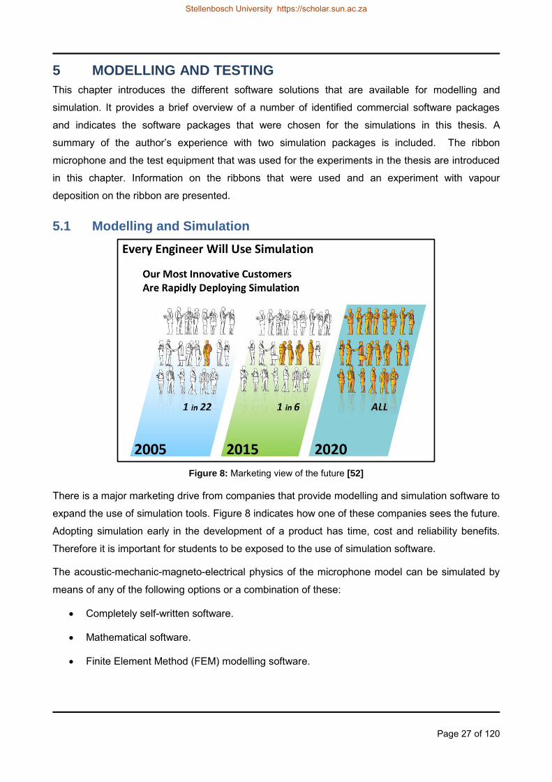
Page 27 of 120
5 MODELLING AND TESTING
This chapter introduces the different software solutions that are available for modelling and
simulation. It provides a brief overview of a number of identified commercial software packages
and indicates the software packages that were chosen for the simulations in this thesis. A
summary of the author‟s experience with two simulation packages is included. The ribbon
microphone and the test equipment that was used for the experiments in the thesis are introduced
in this chapter. Information on the ribbons that were used and an experiment with vapour
deposition on the ribbon are presented.
5.1 Modelling and Simulation
Figure 8: Marketing view of the future [52]
There is a major marketing drive from companies that provide modelling and simulation software to
expand the use of simulation tools. Figure 8 indicates how one of these companies sees the future.
Adopting simulation early in the development of a product has time, cost and reliability benefits.
Therefore it is important for students to be exposed to the use of simulation software.
The acoustic-mechanic-magneto-electrical physics of the microphone model can be simulated by
means of any of the following options or a combination of these:
Completely self-written software.
Mathematical software.
Finite Element Method (FEM) modelling software.
Stellenbosch University https://scholar.sun.ac.za

Page 28 of 120
Writing one‟s own software requires extensive programming experience that falls beyond the
scope of this thesis. Therefore only mathematical and modelling software were considered.
Creating a model with mathematical software still requires a good measure of programming on the
user‟s side though.
In each of these categories both open source and commercial software are available. There is a
myriad of software packages available to choose from. Only a few of the more familiar ones or
those stumbled upon during the work on this thesis are covered here. The following table lists a
few available products that were considered for the simulation of the microphone models.
Table 1: Modelling and simulation products
Open Source Commercial
Mathematical GNU Octave
(www.gnu.org)
Scilab
(www.scilab.org)
MathWorks MATLAB®
(www.mathworks.com)
WOLFRAM Mathematica®
(www.wolfram.com/mathematica)
FEM Clawpack
(www.clawpack.org)
Finite Element Method Magnetics
(www.femm.info)
Altair HyperWorks®
(www.altairhyperworks.com)
COMSOL Multiphysics®
(www.comsol.com)
QuickField
(www.quickfield.com)
ANSYS®
(www.ansys.com)
The open source software requires a much steeper learning curve than the commercial software
and was therefore put aside. The commercial software is discussed below.
5.1.1 Website Calculators
To calculate the force between two magnets or between a magnet and a steel plate the following
online calculator can be used: http://www.kjmagnetics.com/calculator.asp
5.1.2 MathWorks MATLAB® & Simulink®
MATLAB® is the abbreviation for MATrix LABoratory. It is a high-level language used for numeric
computations and visualisation of the results. MATLAB® can be used either to analyse data or to
create models and develop algorithms.
Stellenbosch University https://scholar.sun.ac.za

Page 29 of 120
Simulink® is an environment using block diagrams to create multi-domain simulations and model-
based designs. It also provides automatic generation of software code for embedded systems.
Simulink® is integrated with MATLAB® so that the algorithms in MATLAB® can be imported into
Simulink® models and the simulation results can be exported back to MATLAB® for analysis.
5.1.3 WOLFRAM Mathematica®
Mathematica® uses the Wolfram symbolic language for programming. Equations, code, graphics
and data are all represented as symbolic expressions. It can be used for mathematical
computation, numerical analysis, visualisation of results, algebraic manipulation, number theory,
data analysis, graph computation, image computation, geometric computation and interactive
computation.
5.1.4 Altair Hyperworks®
Altair HyperWorks® is a computer-aided engineering (CAE) and simulation platform used for
modelling and analysis of mostly mechanical designs. It addresses computational fluid dynamics
(CFD) problems in particular, but also offers multi-physics and multi-disciplinary analysis.
HyperWorks® is mainly geared towards the transportation industry for simulation, analysis and
optimization of structural designs, the aerodynamics thereof and impact tests, to name a few.
Since 2014 the South African developed FEKO® electromagnetic analysis software suite is also
falling under the umbrella of Altair®.
5.1.5 COMSOL Multiphysics®
COMSOL Multiphysics® uses finite element analysis (FEA) for physics-based modelling and
simulation. It is a general purpose platform for modelling and simulation of various disciplines,
including electrical, mechanical, chemical and fluid flow for example. COMSOL‟s capability to
model magnetism and electromagnetism with its AC/DC module together with the dedicated
acoustics module makes it the first choice for the topic of a ribbon microphone. COMSOL® makes
it possible to couple the phenomena in these physics domains with one another. COMSOL‟s
LiveLink application interfaces seamlessly with Microsoft Excel, Inventor and MATLAB®. The
interface with Microsoft Excel is handy for loading variables and parameters from lists that can be
generated outside of COMSOL®. The interface with MATLAB® is useful for further analysis of
simulation results. 2D and 3D models can be constructed within COMSOL® with its own geometry
tools. The interface with Inventor is essential for mechanical models that are difficult or impossible
to construct with COMSOL‟s own design module. The application builder feature of COMSOL®
makes it possible to create a user friendly application that hides the complexity of the model while
providing access to selected parameters. These parameters can be manipulated by a user at
another location who needs to observe the model‟s behaviour without necessarily understanding
Stellenbosch University https://scholar.sun.ac.za

Page 30 of 120
the underlying complexities of the model. Horng and Ke [47] [49] used COMSOL® during their work
on the miniaturisation of the ribbon microphone.
5.1.6 ANSYS®
ANSYS® offers engineering simulation software for a wide range of physics including fluids,
structures, electronics, semiconductors, embedded software, and even short duration severe
loadings due to explosions. The ANSYS® simulation software is extremely powerful, but the
drawing tool in ANSYS® is very limited. For best results models have to be created in a CAD
package outside of ANSYS® and then be imported for simulation. ANSYS® is the other simulation
software package that was used for simulations in this thesis.
5.1.7 Software choice
The author identified COMSOL® and ANSYS® as preferred simulation packages because of the
fact that it provides modules for all aspects of the ribbon microphone, i.e. acoustics, mechanics,
magnetics and electromagnetics.
The author‟s experience with these two simulation packages throughout the work for this thesis is
summarised as follow:
COMSOL® is a relatively new product with all the physics modules seamlessly integrated
into a single user interface. Excellent examples for each physics domain are easily found
on the COMSOL® website. The user interface is very intuitive and can be mastered in a
short time by following the step-by-step tutorials and the videos that are freely available
from the COMSOL® website. Local support for the product is very limited however.
ANSYS® consists of a wide suite of mature products that are well integrated to share
information and results amongst each other, but each product still has its own unique user
interface. ANSYS® is in the process of creating a central user interface, but at the time of
this thesis it still had a long way to go. Tutorials are freely available from the ANSYS®
website, but needs a lot of searching to find it inside the huge amount of user support data.
It is difficult to master the ANSYS® user interface if one needs to learn more than one of the
products to perform a multi-physics simulation. This package is for well-seasoned
simulation experts and does not come intuitively. The local support for ANSYS® is however
outstanding. With regular hands-on workshops ANSYS® more than compensates for the
learning barriers.
5.2 Test Equipment
The following hardware and the software were used to perform the experiments described in the
rest of the thesis.
Stellenbosch University https://scholar.sun.ac.za
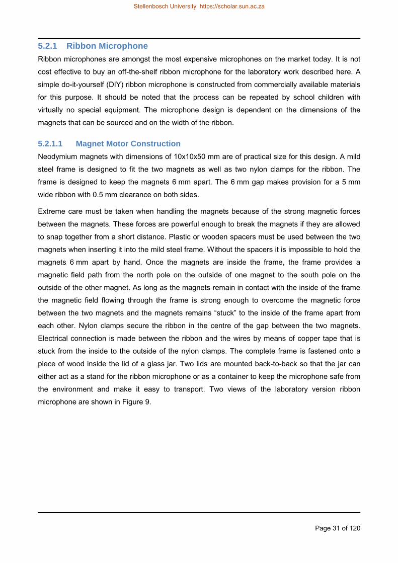
Page 31 of 120
5.2.1 Ribbon Microphone
Ribbon microphones are amongst the most expensive microphones on the market today. It is not
cost effective to buy an off-the-shelf ribbon microphone for the laboratory work described here. A
simple do-it-yourself (DIY) ribbon microphone is constructed from commercially available materials
for this purpose. It should be noted that the process can be repeated by school children with
virtually no special equipment. The microphone design is dependent on the dimensions of the
magnets that can be sourced and on the width of the ribbon.
5.2.1.1 Magnet Motor Construction
Neodymium magnets with dimensions of 10x10x50 mm are of practical size for this design. A mild
steel frame is designed to fit the two magnets as well as two nylon clamps for the ribbon. The
frame is designed to keep the magnets 6 mm apart. The 6 mm gap makes provision for a 5 mm
wide ribbon with 0.5 mm clearance on both sides.
Extreme care must be taken when handling the magnets because of the strong magnetic forces
between the magnets. These forces are powerful enough to break the magnets if they are allowed
to snap together from a short distance. Plastic or wooden spacers must be used between the two
magnets when inserting it into the mild steel frame. Without the spacers it is impossible to hold the
magnets 6 mm apart by hand. Once the magnets are inside the frame, the frame provides a
magnetic field path from the north pole on the outside of one magnet to the south pole on the
outside of the other magnet. As long as the magnets remain in contact with the inside of the frame
the magnetic field flowing through the frame is strong enough to overcome the magnetic force
between the two magnets and the magnets remains “stuck” to the inside of the frame apart from
each other. Nylon clamps secure the ribbon in the centre of the gap between the two magnets.
Electrical connection is made between the ribbon and the wires by means of copper tape that is
stuck from the inside to the outside of the nylon clamps. The complete frame is fastened onto a
piece of wood inside the lid of a glass jar. Two lids are mounted back-to-back so that the jar can
either act as a stand for the ribbon microphone or as a container to keep the microphone safe from
the environment and make it easy to transport. Two views of the laboratory version ribbon
microphone are shown in Figure 9.
Stellenbosch University https://scholar.sun.ac.za

Page 32 of 120
Figure 9: DIY ribbon microphone
5.2.1.2 The Ribbon
Information on a commercial ribbon (Shure Roswellite™) that is the ideal ribbon for laboratory tests
because of its durability is discussed in this paragraph. An attempt to reproduce a similar ribbon in
the laboratory is documented. All the experiments can be performed however, with DIY ribbons
manufactured at home or in the laboratory from inexpensive materials.
The first DIY ribbon is made from light aluminium foil commonly found in a kitchen. Heavy-duty foil
is 20 µm thick and light-duty foil is 10 µm thick. Even the light-duty foil is 5 times thicker than the
ideal ribbon thickness of 2 µm, but for the purposes of this thesis 10 µm is adequate. To obtain a
60 mm long by 5 mm wide ribbon, a 90 mm strip of 5 mm wide aluminium foil can be cut and then
corrugated with the gears from a Lego set.
The second DIY ribbon is manufactured from a piece of thermal space blanket. The thermal
blanket consists of a Polyethylene Terephthalate (PET) film with a thin aluminium deposit on one
side. It is the ability of the aluminium layer to reflect radiated heat that gives the blanket its thermal
properties. Strips of the thermal blanket cannot be corrugated with the Lego gears because it
immediately returns to its original flat form after going through the gears. The only way to corrugate
the PET strips is to form it in a jig and then bake it in the jig at 90º C for an hour. In this process
Stellenbosch University https://scholar.sun.ac.za

Page 33 of 120
special care must be taken not to damage the thin aluminium coating. The product of the baking
process is a corrugated ribbon with the ability to return to its corrugated form after being stretched
out to its original length.
Shure Incorporated owns the intellectual property for a shape-memory ribbon material called
Roswellite™. It was developed by Soundwave Research but Shure got the rights to it when they
acquired Crowley and Tripp Ribbon Microphones from Soundwave Research Laboratories in 2009
[53]. Roswellite™ is a replacement for the aluminium foils that are normally used in ribbon
microphones. Shure claims it to be a “nano-enabled ribbon material” that is much more durable
than metal foils [54]. The claim that it is more durable is true, but it has nothing to do with nanotube
technology. Unless Shure has deviated substantially from their patent application [45], these
ribbons are simply made from a thin polymer (e.g. 2.5 µm PET) that is coated with a layer of
conductive material like aluminium or gold.
The ribbon of a ribbon microphone can be easily damaged during experimentation. To replace a
2 µm aluminium foil ribbon is a very delicate process that would rather be avoided. Therefore it is
desirable to conduct all experiments by using a custom made ribbon that has similar properties to
Roswellite™. An attempt was made to manufacture a Roswellite™-like ribbon by depositing 1 µm
(10 000 Ångstrom) of aluminium onto pieces of Mylar™, Polypropylene and PET film. Mylar™
would make an excellent ribbon. It is used in certain dynamic microphones for its unique qualities.
Mylar™ is a polyester film manufactured by DuPont. It is extremely durable, has high tensile
strength, can withstand extreme temperatures (-40ºC to +170ºC) and has half the weight of
aluminium [22]. It also has a long lasting flex life. When formed under high temperature and
pressure its molecular structure changes permanently. The shape memory will cause it to return to
its shaped form even after large temporary deformations. Mylar™ will therefore produce a gust
proof ribbon. It only has to be coated with a thin layer of conductive material to add the required
electromagnetic properties.
The engineering department of the university has vapour deposition equipment that can be used to
deposit various metals onto other substrates. Aluminium was deposited at an evaporation rate of
5 Å/s for a duration of 33 minutes to deposit a 10 kÅ thin layer. The Mylar™ and Polypropylene
were visibly affected by the heat of the vapour deposition process. The PET showed little adverse
effects to the heat (Figure 10). The resistance of the ribbon can be calculated as:
(1)
where is the resistance in ohm, the resistivity constant of the material in Ω/m, the length
in m and the cross-sectional area in m2. The resistivity of aluminium is 2.82 x 10⁻⁸ Ω/m.
The resistance of this ribbon should be 0.325 Ω for a ribbon length of 50 mm, width of 4 mm and
thickness of 1.0 µm. After the vapour deposition however, the resistance of the aluminium layers
Stellenbosch University https://scholar.sun.ac.za

Page 34 of 120
on all the polymers were measured to be in the kilo-ohm range, which is much too high for 1 µm of
aluminium. The colour of the aluminium layer was not bright and shiny like a mirror, but brownish.
The aluminium layer also allowed much light through. The high resistance, brownish colour and
transparency of the aluminium led the author to believe that impurities were present in the
evaporation chamber during the evaporation process. The impurities will lead to poor cohesion of
the aluminium molecules and poor adhesion to the substrate. The impurity molecules that are also
deposited along with the aluminium will cause electrical insulation between the aluminium
molecules. On close inspection an oily substance was found on the sensor arm of the vapour
deposition system. This oily substance may explain the impurities that were present in the
chamber. After further investigation it turned out that the vapour deposition equipment was faulty
and it would take a considerable amount of time before the equipment would be repaired. No
further attempts were made at vapour deposition. Photos of the vapour deposition equipment are
shown in Figure 11.
Figure 10: Vapour deposition of aluminium onto PET (left), Mylar™ (centre) and Polypropylene (right)
The upper frequency range of the ribbon microphone is limited by the length of the path from the
front to the back of the ribbon and not by the ribbon thickness (up to a reasonable point). According
to Artur Fisher the reason why thinner ribbons tends to sound better is because of the transient
response of the ribbon [55]. In musical definition it affects the attack of the sound. In other words, it
produces a brighter sound. These transients are especially important in the reproduction of the
sounds of percussion instruments, symbols and acoustic guitars. In this thesis the subtleties of
these transients are not investigated. Therefore the 10 µm aluminium and the space blanket
ribbons are sufficient.
Stellenbosch University https://scholar.sun.ac.za
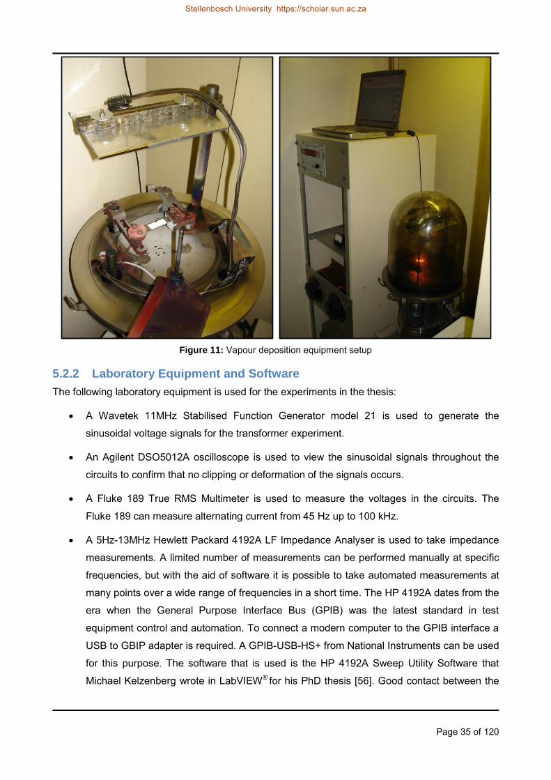
Page 35 of 120
Figure 11: Vapour deposition equipment setup
5.2.2 Laboratory Equipment and Software
The following laboratory equipment is used for the experiments in the thesis:
A Wavetek 11MHz Stabilised Function Generator model 21 is used to generate the
sinusoidal voltage signals for the transformer experiment.
An Agilent DSO5012A oscilloscope is used to view the sinusoidal signals throughout the
circuits to confirm that no clipping or deformation of the signals occurs.
A Fluke 189 True RMS Multimeter is used to measure the voltages in the circuits. The
Fluke 189 can measure alternating current from 45 Hz up to 100 kHz.
A 5Hz-13MHz Hewlett Packard 4192A LF Impedance Analyser is used to take impedance
measurements. A limited number of measurements can be performed manually at specific
frequencies, but with the aid of software it is possible to take automated measurements at
many points over a wide range of frequencies in a short time. The HP 4192A dates from the
era when the General Purpose Interface Bus (GPIB) was the latest standard in test
equipment control and automation. To connect a modern computer to the GPIB interface a
USB to GBIP adapter is required. A GPIB-USB-HS+ from National Instruments can be used
for this purpose. The software that is used is the HP 4192A Sweep Utility Software that
Michael Kelzenberg wrote in LabVIEW® for his PhD thesis [56]. Good contact between the
Stellenbosch University https://scholar.sun.ac.za

Page 36 of 120
analyser adapter and the item under test is very important. To obtain the best possible
contact, short pieces of silver wire is soldered onto the transformer wires before performing
the measurements.
A set of low cost Logitech S-220 speakers is used for the acoustic tests. The set consists of
an active subwoofer with built-in amplifier and a pair of stereo speakers.
Many of the tests are performed with the aid of John Mulcahy‟s Room EQ Wizard (REW).
The software is intended for acoustic analysis of room and loudspeaker response, but it
works equally well for turning a personal computer (PC) or laptop with soundcard into a
laboratory tool. REW may be downloaded free of charge from www.roomeqwizard.com to
be used within the (very lenient) restrictions of its licensing agreement.
5.2.3 Acoustic Environment
Ideally all acoustic tests should be performed in a room with sound absorbing and damping
material that prevents reflected sound waves from influencing the test results. For the thesis
however no special arrangements were made to the acoustic environment. The idea is to have an
acoustic environment that students can quite easily arrange themselves. All acoustic tests were
performed with a speaker relatively close to the microphone so that any reflected sound waves
would be small compared to the intensity of the sound waves from the speaker itself.
Stellenbosch University https://scholar.sun.ac.za

Page 37 of 120
6 ACOUSTICS
The first of the physics areas for which the ribbon microphone can be used eminently as
demonstration tool, is that of acoustics. The propagation of a wave in space, phenomena such as
reflection and interference caused by the physical structure of the microphone, the behaviour of the
wave as a function of frequency, and concepts like phase differences in space can be coupled
seamlessly with the working and properties of the microphone, especially when using modelling
software for complex analysis and graphical visualization. While a sound wave in an
obstructionless, ideal environment can be modelled by a simple mathematical formula, the
movement of an object due to such a wave is much more sophisticated, as size, weight, elasticity
and orientation all play a role. As this problem is at the heart of the ribbon microphone operation,
analysis of such a structure serves well to illustrate behaviour of acoustic waves in the vicinity of
obstacles, and its effect on a small obstacle. This is normally far beyond what can be illustrated
with simple mathematical models, and provides significant additional insight.
In addition, modelling aspects such as meshing, computer limitations, etc. is well illustrated by this
problem. This area of engineering education (i.e. use of modelling software) has become extremely
important, and the extreme ranges required for the analysis of microphones forms a perfect vehicle
for illustrating this.
This chapter presents 8 experiments which can be performed using a basic ribbon microphone as
simulation model.
A set of simulation experiments modelling objects of varying size, weight and elasticity in an
acoustic wave. Here the focus is on the movement and deformation of the object, with the
object constituting a small section of a ribbon. The aim here is to illustrate mainly the
dynamic movement of solids in waves.
Experiments showing the effects of meshing on solutions. These are of a more advanced
nature, and it is presented here since computer simulation is currently introduced into
engineering courses from a very early stage, and problems with meshing can create
completely false results.
Experiments showing the influence of a solid object on an acoustic wave. Here, the focus is
on the wave, and how it is affected by obstacles over the very wide frequency range
of 1:1000.
No physical experiments are done in this chapter since its main purpose is to demonstrate the
power of modelling and simulation and to highlight a number of challenges in simulation.
Stellenbosch University https://scholar.sun.ac.za

Page 38 of 120
6.1 Theory
Sound waves are longitudinal waves, but for illustration purposes it is often drawn as transverse
waves as illustrated in Figure 12. The crests on the transverse wave represent the high pressure
sections of the longitudinal wave (dense, compression of particles) and the troughs represent the
low pressure sections (sparse, rarefaction of particles).
Figure 12: Transverse wave representation of a longitudinal sound wave
A simple periodic sound wave in an elastic medium can be described by the wave function
(2)
where is the displacement from equilibrium of a particle in position at a moment in time.
is the maximum displacement and the propagation constant. The angular frequency equals
(where is the frequency). The value of may be large when illustrating wave motion by
means of a string or a coil, but for a sound wave in air the value of is in the nanometre range.
The theoretical maximum distance ( ) that a weightless particle will be displaced in a sound
wave can be calculated as
(3)
where is the density of the medium, the speed of sound, the angular frequency
and
√ (4)
with the intensity level of the sound wave in W/m2 [57].
Stellenbosch University https://scholar.sun.ac.za

Page 39 of 120
From (3) it can be seen that the particle‟s displacement is directly proportional to the pressure
difference and inversely proportional to the frequency.
Combining (3) and (4) into one equation gives
√
(5)
To illustrate the tiny magnitudes that are involved when air particles are displaced in a sound wave,
the displacement is calculated for two extreme scenarios:
The threshold of hearing (1x10-12 W/m2, i.e. 20 µPa or 0 dB), i.e. the intensity of the faintest 1 kHz pure tone that can be detected by the human ear, and
The threshold of pain (1 W/m2, i.e. 20 Pa or 120 dB), i.e. the upper limit for human hearing.
With the speed of sound equal to 343 m/s in air (at 20ºC), the density of air equal to 1.2 kg/m3 and
a frequency of 1 kHz, (5) yields a displacement of at the threshold of hearing and a
displacement of at the threshold of pain.
Comprehending that the displacement of an air particle at 120dB is one million times larger than
the displacement at the lower threshold of hearing, it is no wonder that sound this loud hurts the
inner ear regardless of all the damping mechanisms inside the ear.
The relationship between the displacement, velocity and acceleration of a particle in a sound wave
is shown in Figure 13 [22].
Figure 13: Relationship between particle displacement, velocity and acceleration [22]
Stellenbosch University https://scholar.sun.ac.za

Page 40 of 120
From Figure 13 it is notable that the electrical output of the ribbon microphone is at its peak
amplitude when the movement of the ribbon is at its highest velocity. It can thus be seen that the
electrical signal lags the displacement of the air particles by 90 degrees.
6.1.1 Magnitude of a Sound Wave
The magnitude of a sound wave is expressed in various terms throughout literature. One way to
express it is in terms of its energy and it is called sound intensity or acoustic intensity. Otherwise
the term sound pressure is used to express it as a function of its force.
Sound Intensity
Sound intensity is the energy transmitted per unit of time (i.e. power), in a specific direction,
through a unit area that is positioned perpendicular to the direction of propagation [58].
Sound intensity is expressed in watts per square metre (W/m2) [59].
Sound Pressure
Sound pressure is the force that a sound wave exerts per unit area. Although force is a vector,
pressure is a scalar quantity.
Pressure is expressed either in Newton per square metre (N/m2), or in Pascal (Pa) [57].
Due to the fact that the dynamic range of human hearing stretches over such a wide range
(typically 1x10-12 W/m2 to 1 W/m2), sound pressure and sound intensity are not commonly
expressed in W/m2 or N/m2, but rather as a ratio relative to a certain reference level. The reference
level that has been chosen in both cases is the lower threshold of human hearing, i.e. the faintest
sound of a 1 kHz pure tone that can be distinguished by a healthy young adult. In terms of intensity
this level is 1x10-12 W/m2 and in terms of pressure it is 20x10-6 Pa. Because the ratios are so large,
it is expressed on a logarithmic scale. The unit that is used is the decibel (dB). The decibel is not a
measuring unit in a physical sense but only a reference to the logarithmic ratio definition.
The sound intensity level in dB is defined as
(
) (6)
where = 1x10-12 W/m2.
The sound pressure level in dB is defined as
(
) (7)
where is the root mean square pressure and equals 20 µPa [60].
Stellenbosch University https://scholar.sun.ac.za

Page 41 of 120
The sound pressure level is defined differently from sound intensity because the pressure ratio
equals the square root of its corresponding power ratio [58].
The outputs of microphones produce voltage outputs that are proportional to the pressure of the
sound waves. Therefore in practice, sound pressure levels (SPL) are more widely used than sound
intensity levels [59].
6.1.2 Mathematical Models for Acoustic Analysis
In this paragraph an overview is provided of the acoustic theory that is required for the simulation
of acoustic models. This information was obtained from [61].
6.1.2.1 Frequency Domain Studies
In standard acoustic problems the small variations in the acoustic pressure on top of a stationary
background pressure must be solved. The following two equations form the basis for a lossless
(i.e. no thermal conduction and no viscosity) compressible fluid flow problem:
1. The momentum equation (Euler):
(8)
2. The continuation equation:
(9)
where is the total density, total pressure, velocity field.
The thermodynamic processes are assumed to be adiabatic and reversible, i.e. isentropic
processes. The small parameter expansion is performed at a pressure (in Pascal) on a
stationary fluid with density of (in kilogram per cubic metre) in a way that the following apply:
where and (the primed variables indicate the small acoustic variations).
Inserting these expressions into the base equations and keeping only the terms that are linear in
the primed variables lead to the following:
(10)
(11)
Stellenbosch University https://scholar.sun.ac.za

Page 42 of 120
Density is a dependent variable and can therefore be eliminated by expressing it through
linearization (1st order Taylor expansion):
(12)
where is the speed of sound at constant entropy .
Rearranging the equations and dropping the primes lead to the following equation for sound waves
in a lossless medium:
(
) (13)
where is the bulk modulus (N/m2) of the medium, the dipole source (N/m3) and the
monopole source (1/s2), showing that the speed of sound in a fluid is related to its compressibility.
A wave for which the pressure changes over time (time-harmonic wave) can be expressed as:
(14)
where (rad/s) with the frequency in Hertz.
Taking this time-harmonic wave and assuming the same time dependence for its source, the wave
equation can be reduced to an inhomogeneous Helmholtz equation:
(
)
(15)
This is the equation that COMSOL® solves for frequency domain studies of 3D geometries.
6.1.2.2 Eigen Frequency Study
The solutions of the wave equation will be limited to a series of discrete functions (Eigen functions)
when boundary conditions are applied to the system. Eigen functions are also known as the
normal modes of the system. A unique frequency is associated with the solution of each mode.
This frequency is known as the Eigen frequency or natural frequency. The normal mode with the
lowest Eigen frequency is known as the fundamental mode. The frequency associated with this
mode is called the fundamental (first) harmonic. The rest of the Eigen frequencies (second, third,
fourth, etc. harmonics) are called overtones [59].
One or more of the following boundary conditions may be applied to the wave equation or the
Helmholtz equation:
Sound hard boundary or wall, where the acceleration of the normal component is zero
Stellenbosch University https://scholar.sun.ac.za

Page 43 of 120
(
) (16)
Sound soft boundary, where the acoustic pressure disappears ( ).
Impedance boundary, where represents the impedance somewhere between a hard
boundary ( ) and a soft boundary ( )
(
)
(17)
Radiation boundary or perfectly matched layer, with minimal reflections to the model (an
unbounded open domain).
The attenuation of sound waves in a medium where losses occur is modelled by adding a first
order time derivative with a damping coefficient
(
) (18)
(15) can be used to solve the Eigen modes and Eigen frequencies of the acoustic problem by
removing the two source terms, yielding the equation:
(
)
(19)
where . In other words, the eigenvalue is related to the Eigen frequency
and the angular frequency .
6.2 Modelling and Simulation
Sound waves are useful for an introduction to wave theory, as points of low and high pressure can
be heard by the human ear. Also, the behaviour of sound wave particles is easier to visualise than
for instance electromagnetic waves.
To get an idea of the maximum distance a ribbon may travel in sound waves of different
frequencies and to see how it compares to the theoretical displacement of a weightless particle, a
small element of extremely low mass is placed freely inside a modelling sphere.
The model consists of a small flat disk (10 µm thin, with 25 mm radius) suspended freely in the
path of a sound wave. The modelling domain is enclosed in a sphere with 40 mm radius. The disk
is positioned on the x-z plane with its thickness in the direction of the y-axis. The model is shown in
Figure 14.
Stellenbosch University https://scholar.sun.ac.za

Page 44 of 120
Figure 14: Model of free floating disk inside a sphere (the modelling domain)
During the simulation a number of obstacles and challenges were encountered that will be
discussed in the paragraphs to follow.
6.2.1 Selecting the Sound Level
The incident sound wave is modelled as a plane wave travelling in the positive y-direction. The
pressure of the sound wave is 1 Pa (≈ 94 dB).
(
) (20)
where is the sound pressure level in dB, is the pressure of the sound in Pascal and is
the reference pressure equal to 20 µPa.
A sound level of 94 dB is very loud, but realistic compared to the voice intensity of an opera singer
at a distance of 30 cm from the microphone [62]. Although the dynamic range of a singer‟s voice at
this level is only between 300 Hz and 1.2 kHz, the same pressure will be used for modelling all
frequencies up to 20 kHz. At lower intensities the dynamic range of a singer‟s voice is much wider.
Human perception of frequency is dominated by hearing. To put audible frequencies into
perspective: The frequency of middle-C on a piano is tuned to 261.63 Hz and the frequency of the
C-key two octaves higher is 1 046.52 Hz. The fundamental frequency of the notes on a standard
88-key piano ranges from 27.5 Hz on the low end to 4 186 Hz on the high end [63].
Stellenbosch University https://scholar.sun.ac.za

Page 45 of 120
6.2.2 Narrow Faces
This experiment illustrates the importance of handling extreme ratios in simulations.
Generating a mesh for the model becomes troublesome when extreme differences in dimensions
exist within the model. A particle of only 2 um thick in a sphere with a 40 mm radius presents such
a dilemma with its one-to-twenty-thousand ratio between small and large dimensions. A method is
provided to deal with these extremities by deleting narrow faces from the model. To test the effect
of deleting the narrow faces, a model that is on the edge of the large ratio dilemma is chosen and
simulated with narrow faces and without narrow faces. The model chosen consists of a 10 um thick
disk, with a radius of 2.5 mm, hit by a plane wave with a sound pressure level of 1 Pa (94dB). The
simulation is performed over a frequency range of 500 Hz to 1 kHz. Figure 15 and Figure 16
provide a comparison between the two simulations. The coloured lines in the figures represent a
cut along the z-axis through the centre of the free floating disk in Figure 14, showing the
displacement of the disk at different frequencies.
Figure 15: Free floating disk with narrow faces, 500 Hz to 1 kHz
From the displacement plots in the two figures it is clear that there is a considerable difference
between the simulation results of the two models (30% at 700 Hz). The model without narrow faces
gives a mean displacement value of 52x10-9 m at 700 Hz and the model that includes the narrow
faces is only displaced by 40x10-9 m. The equation in (5) yields a displacement value of
794x10-9 m at 700 Hz for a weightless particle in a 94 dB sound wave (i.e. sound intensity of
2.512x10⁻³ W/m2). The results from both simulations are so far below the theoretical maximum
displacement that the theoretical value cannot be used to deduce which of the two simulation
models is the better. The large difference between the theoretical and the simulated values can be
ascribed to the inertia of the disk. The influence of the disk‟s weight is further analysed in 6.2.4.
Stellenbosch University https://scholar.sun.ac.za
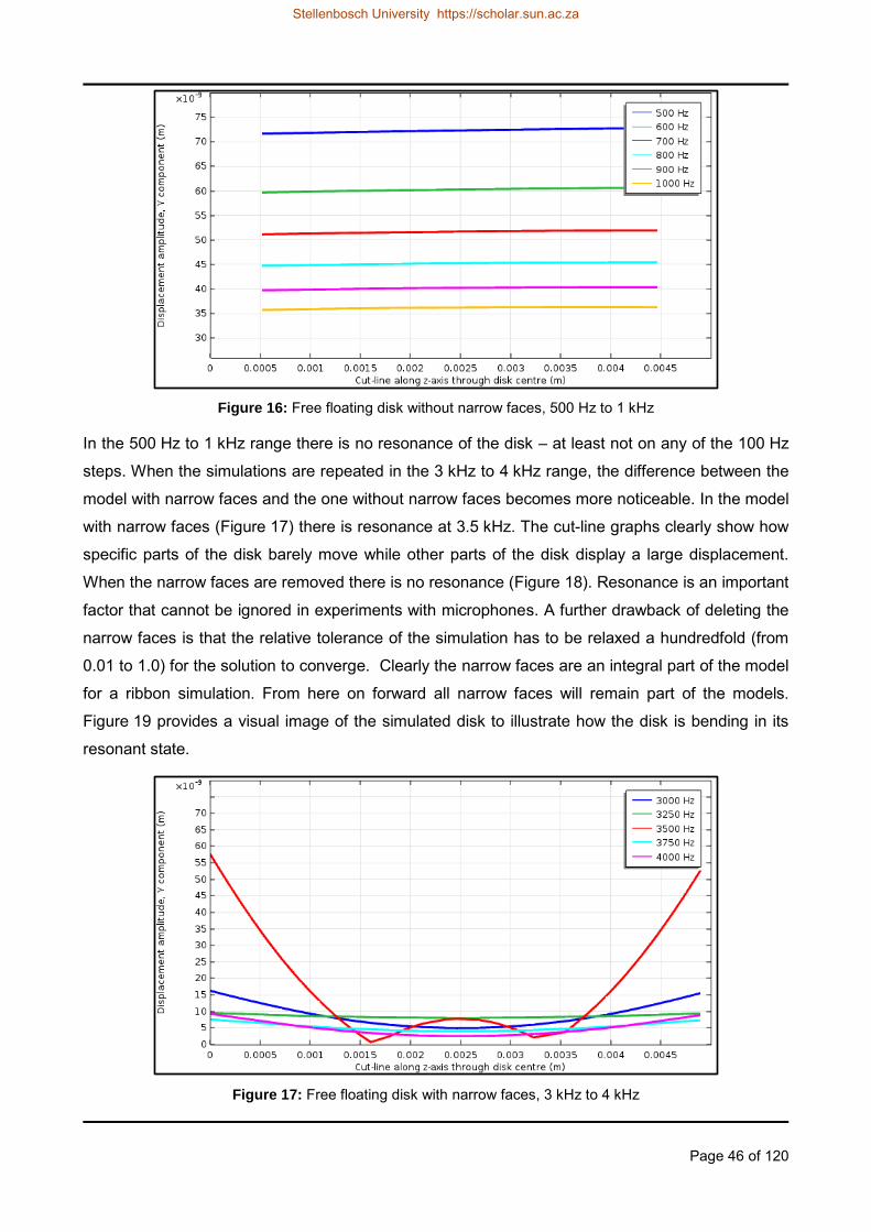
Page 46 of 120
Figure 16: Free floating disk without narrow faces, 500 Hz to 1 kHz
In the 500 Hz to 1 kHz range there is no resonance of the disk – at least not on any of the 100 Hz
steps. When the simulations are repeated in the 3 kHz to 4 kHz range, the difference between the
model with narrow faces and the one without narrow faces becomes more noticeable. In the model
with narrow faces (Figure 17) there is resonance at 3.5 kHz. The cut-line graphs clearly show how
specific parts of the disk barely move while other parts of the disk display a large displacement.
When the narrow faces are removed there is no resonance (Figure 18). Resonance is an important
factor that cannot be ignored in experiments with microphones. A further drawback of deleting the
narrow faces is that the relative tolerance of the simulation has to be relaxed a hundredfold (from
0.01 to 1.0) for the solution to converge. Clearly the narrow faces are an integral part of the model
for a ribbon simulation. From here on forward all narrow faces will remain part of the models.
Figure 19 provides a visual image of the simulated disk to illustrate how the disk is bending in its
resonant state.
Figure 17: Free floating disk with narrow faces, 3 kHz to 4 kHz
Stellenbosch University https://scholar.sun.ac.za

Page 47 of 120
Figure 18: Free floating disk without narrow faces, 3 kHz to 4 kHz
Figure 19: Disk resonance illustrated at 3.5 kHz (simulated with narrow faces)
6.2.3 Mesh Density
This experiment illustrates the importance of choosing the best mesh in simulations.
For this experiment the model of Figure 17 is used and the mesh density is halved in the
y-direction. See Figure 20 for a visual comparison of the two meshes and Figure 21 for the
displacement results of the simulation. It is noticeable that the resonant frequency becomes less
dominant. The mesh resolution and the element quality are important considerations. When the
mesh resolution is low in comparison to variations in the geometry or the solution, it will lead to
inaccurate results. A low mesh element quality may lead to inverted mesh elements with
misleading results. It may also prevent the solution from converging. Thus, the mesh must be as
fine as reasonably possible, subject to the processing capabilities of the computer that is used to
run the simulation and also time permitting since the simulation with a finer mesh takes much
longer to compute. See Figure 23 in the next experiment for an additional example of the influence
that different mesh settings have on the simulation results.
Stellenbosch University https://scholar.sun.ac.za
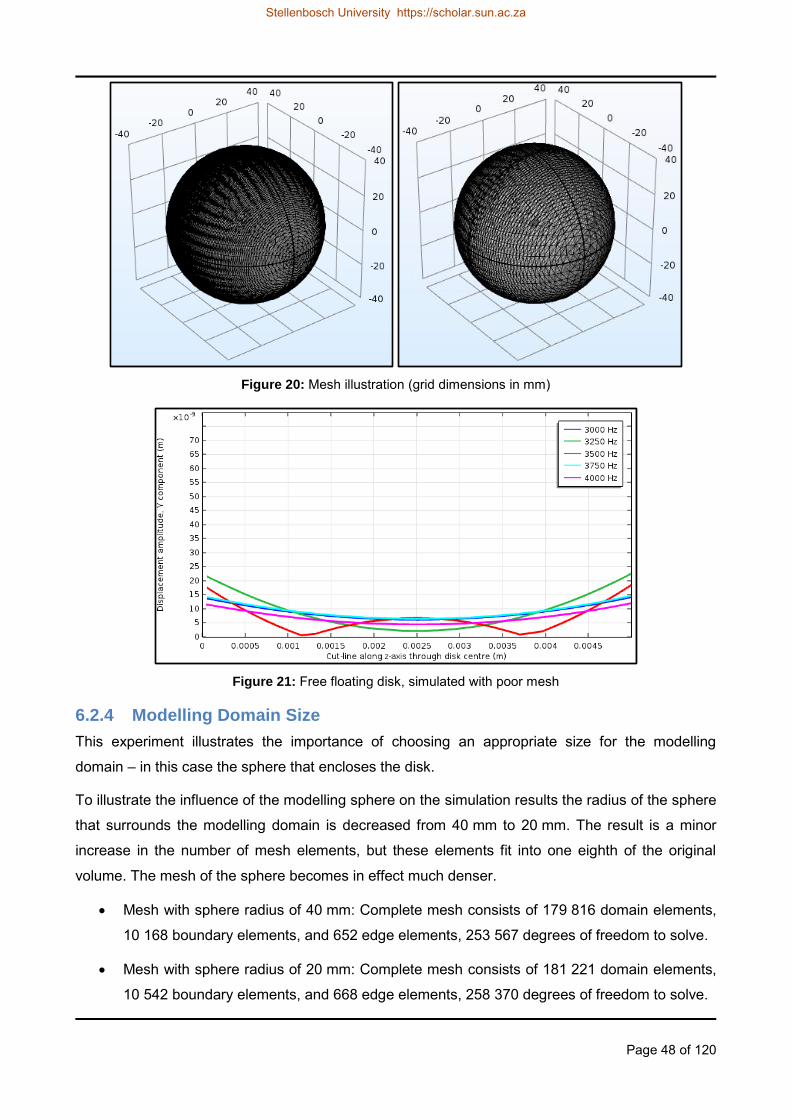
Page 48 of 120
Figure 20: Mesh illustration (grid dimensions in mm)
Figure 21: Free floating disk, simulated with poor mesh
6.2.4 Modelling Domain Size
This experiment illustrates the importance of choosing an appropriate size for the modelling
domain – in this case the sphere that encloses the disk.
To illustrate the influence of the modelling sphere on the simulation results the radius of the sphere
that surrounds the modelling domain is decreased from 40 mm to 20 mm. The result is a minor
increase in the number of mesh elements, but these elements fit into one eighth of the original
volume. The mesh of the sphere becomes in effect much denser.
Mesh with sphere radius of 40 mm: Complete mesh consists of 179 816 domain elements,
10 168 boundary elements, and 652 edge elements, 253 567 degrees of freedom to solve.
Mesh with sphere radius of 20 mm: Complete mesh consists of 181 221 domain elements,
10 542 boundary elements, and 668 edge elements, 258 370 degrees of freedom to solve.
Stellenbosch University https://scholar.sun.ac.za
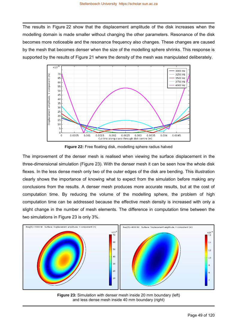
Page 49 of 120
The results in Figure 22 show that the displacement amplitude of the disk increases when the
modelling domain is made smaller without changing the other parameters. Resonance of the disk
becomes more noticeable and the resonance frequency also changes. These changes are caused
by the mesh that becomes denser when the size of the modelling sphere shrinks. This response is
supported by the results of Figure 21 where the density of the mesh was manipulated deliberately.
Figure 22: Free floating disk, modelling sphere radius halved
The improvement of the denser mesh is realised when viewing the surface displacement in the
three-dimensional simulation (Figure 23). With the denser mesh it can be seen how the whole disk
flexes. In the less dense mesh only two of the outer edges of the disk are bending. This illustration
clearly shows the importance of knowing what to expect from the simulation before making any
conclusions from the results. A denser mesh produces more accurate results, but at the cost of
computation time. By reducing the volume of the modelling sphere, the problem of high
computation time can be addressed because the effective mesh density is increased with only a
slight change in the number of mesh elements. The difference in computation time between the
two simulations in Figure 23 is only 3%.
Figure 23: Simulation with denser mesh inside 20 mm boundary (left) and less dense mesh inside 40 mm boundary (right)
Stellenbosch University https://scholar.sun.ac.za
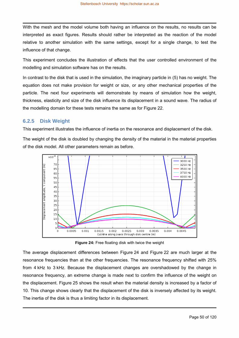
Page 50 of 120
With the mesh and the model volume both having an influence on the results, no results can be
interpreted as exact figures. Results should rather be interpreted as the reaction of the model
relative to another simulation with the same settings, except for a single change, to test the
influence of that change.
This experiment concludes the illustration of effects that the user controlled environment of the
modelling and simulation software has on the results.
In contrast to the disk that is used in the simulation, the imaginary particle in (5) has no weight. The
equation does not make provision for weight or size, or any other mechanical properties of the
particle. The next four experiments will demonstrate by means of simulation how the weight,
thickness, elasticity and size of the disk influence its displacement in a sound wave. The radius of
the modelling domain for these tests remains the same as for Figure 22.
6.2.5 Disk Weight
This experiment illustrates the influence of inertia on the resonance and displacement of the disk.
The weight of the disk is doubled by changing the density of the material in the material properties
of the disk model. All other parameters remain as before.
Figure 24: Free floating disk with twice the weight
The average displacement differences between Figure 24 and Figure 22 are much larger at the
resonance frequencies than at the other frequencies. The resonance frequency shifted with 25%
from 4 kHz to 3 kHz. Because the displacement changes are overshadowed by the change in
resonance frequency, an extreme change is made next to confirm the influence of the weight on
the displacement. Figure 25 shows the result when the material density is increased by a factor of
10. This change shows clearly that the displacement of the disk is inversely affected by its weight.
The inertia of the disk is thus a limiting factor in its displacement.
Stellenbosch University https://scholar.sun.ac.za

Page 51 of 120
Figure 25: Free floating disk, 10 times the weight
6.2.6 Disk Thickness
This experiment illustrates the influence of geometry on the resonance and displacement of the
disk.
Figure 26 shows the simulation results for a disk that is double as thick as the original disk. A
comparison with Figure 22 indicates that the displacement is now less than half of what it was. The
reason is two-fold: the thicker disk is heavier and it is also more rigid. Although the thicker disk is
the same weight than the disk that was used in Figure 24, the displacement is not the same. The
thicker disk displays no resonance in this frequency band because it is more rigid than the original
disk. It illustrates that the displacement of an object is much lower when it does not resonate.
Figure 26: Free floating disk twice as thick, original density
To isolate the disk thickness as the only change in the model, the weight of the disk is reduced to
its original weight by halving the material density. The result of a thicker disk with the same weight
than the original disk is shown in Figure 27. This result confirms that the thicker disk does not
Stellenbosch University https://scholar.sun.ac.za

Page 52 of 120
resonate in the frequency band between 3 kHz and 4 kHz. The displacement of the disk in
Figure 27 is double the displacement of the disk in Figure 26. This supports the conclusion of the
previous experiment about the inertia of the disk.
Figure 27: Free floating disk twice as thick, original weight
6.2.7 Disk Elasticity
This experiment illustrates the influence of elasticity on the resonance frequency and the
displacement of the disk. The disk is not perfectly rigid and can therefore be used to illustrate how
an object deforms when subjected to stimuli at its natural resonance modes.
The elasticity of the disk can be manipulated by changing the Young‟s modulus of the material that
the disk is made of. When the Young‟s modulus of the disk is doubled, the disk becomes more
rigid and the model behaves as in Figure 28.
Figure 28: Free floating disk, less elastic
Comparing to Figure 27 the mean magnitude of the displacement is the same, but the disk is
bending slightly more. The disk is not as rigid as a disk that is twice the thickness, but it is rigid
Stellenbosch University https://scholar.sun.ac.za

Page 53 of 120
enough to shift the resonance frequency out of this band. Making the disk more elastic, has the
opposite effect, as illustrated in Figure 29. The material properties that influence a material‟s
resistance to deformation are listed here for reference [57]:
Young‟s modulus: A measure of a material‟s resistance to change in its length.
Shear modulus: A measure of a material‟s resistance to movement of parallel planes within
the material.
Bulk modulus: A measure of a material‟s resistance to change in its volume when a force
of uniform magnitude is applied perpendicular over the total surface of the object.
Figure 29: Free floating disk, more elastic
6.2.8 Disk Radius
This experiment illustrates the influence that the total area of the disk has on its resonance
frequency and the displacement of the disk.
For Figure 30 the disk‟s radius is increased to double the original radius. The result with the larger
radius is higher displacement amplitude – double the mean amplitude compared to Figure 22. The
reason for this behaviour is that the wave front now has an impact on a surface area that is four
times larger. The larger surface area of the disk has a greater positive impact on its response than
the negative effect of the increased inertia.
To isolate the disk radius as the only change in the model, the weight of the disk is reduced to its
original weight. Figure 31 clearly illustrates how the displacement of the disk increases with the
increased area. The overall rigidity of the disk is lower because of the increased area. Therefore
the disk is bending much more in the sound wave.
Stellenbosch University https://scholar.sun.ac.za

Page 54 of 120
Figure 30: Free floating disk of double the radius, original density
Figure 31: Free floating disk of double the radius, original weight
6.2.9 Final Model for the Free Floating Disk
For the final disc illustration a model is created with a disk that is the thickness of the ideal ribbon.
The radius is kept at 2.5 mm because a diameter of 5 mm corresponds to the width of most
commercial ribbons. The ideal thickness of a microphone ribbon is 2 µm according to literature.
This is only 20% of the thickness of the disk in the preceding simulations. So there has to be a
change in the model to get the mesh right and to get the simulation to converge to a solution.
Reducing the radius of the modelling sphere to 10 mm provides a mesh that accommodates the
2 µm thin disk. The simulation result is presented in Figure 32.
Stellenbosch University https://scholar.sun.ac.za

Page 55 of 120
Figure 32: Free floating disk, 2 µm aluminium, modelling sphere radius 10 mm
The final assembly of the microphone will however not fit in a sphere this small, so another solution
needs to be found to accommodate a 2 µm ribbon. The mesh densities of the disk and the
modelling sphere can be manipulated individually. The disk is positioned with its thickness in the
direction of the y-axis. Consequently, the mesh density is increased in the y-direction only. By
increasing the y-direction mesh scale of the disk from 10 to 50 and the mesh scale of the sphere
from 10 to 20 a combination is found that produces a mesh without errors for the 40 mm sphere.
The result of the 40 mm sphere with 2 µm disk that is simulated with this mesh combination is
presented in Figure 33. The consequence of the compromise that is made with the mesh can be
seen in the surface plot along the cut-line of the disk. It is clear in the 3D representation of
Figure 32 that the displacement of the disk is perfectly concentric as would be expected, but the
3D displacement in Figure 33 is not perfect. Because of the denser mesh in such a large volume
the simulation has to be solved for more degrees of freedom. In this example it takes 50% longer
to compute the results for the model in Figure 33 than to solve the model for Figure 32.
Figure 33: Free floating disk, 2 µm thin, modelling sphere radius 40 mm
Stellenbosch University https://scholar.sun.ac.za

Page 56 of 120
6.2.10 Impact of the Microphone Baffle on a Sound Wave
The microphone magnets are modelled by two rectangular bars inside a sphere. The purpose of
the sphere is to limit the size of the model to the area of interest. The simulation software makes
use of artificial boundaries to mimic an open field within the limited size model. In this case a
Spherical Wave Radiation node is used to add a radiation boundary condition which allows
outgoing spherical waves to leave the model with minimal reflections. Therefore the microphone
baffle (mechanical structure and magnets) is modelled as if it exists in an open field with almost no
reflection from any surroundings. The magnets are completely solid compared to the density of air.
Therefore the baffle parts are modelled as Interior Sound Hard Boundary (Wall) entities. No
deformation of the baffle is taken into account.
Olson stated that the upper frequency of the ribbon microphone is limited by the path length
around the baffle of the microphone [28]. In the simulation model, the neodymium magnets
themselves are forming the baffle. To visualise the influence of the baffle on an incoming sound
wave, the microphone with ribbon is modelled and a simulation is done to illustrate the sound
pressure on the x-y plane through the centre of the microphone. A frequency of 20 kHz is chosen
for the simulation because it is the upper frequency of human hearing and the wavelength
(17.15 mm) fits well inside the modelling sphere for visualisation purposes. In Figure 34 it is clearly
shown how the sound wave bends around the magnets and that the path length around the
magnets are longer than the wavelength of the 20 kHz sound wave. The displacement of the
ribbon is also visible and will be covered in more detail in paragraph 7. Figure 35 provides more
views for the same model. In this model the sound wave is travelling in the positive x-direction.
Figure 34: Ribbon microphone in a 20 kHz sound wave [1] © 2016 IEEE
Stellenbosch University https://scholar.sun.ac.za
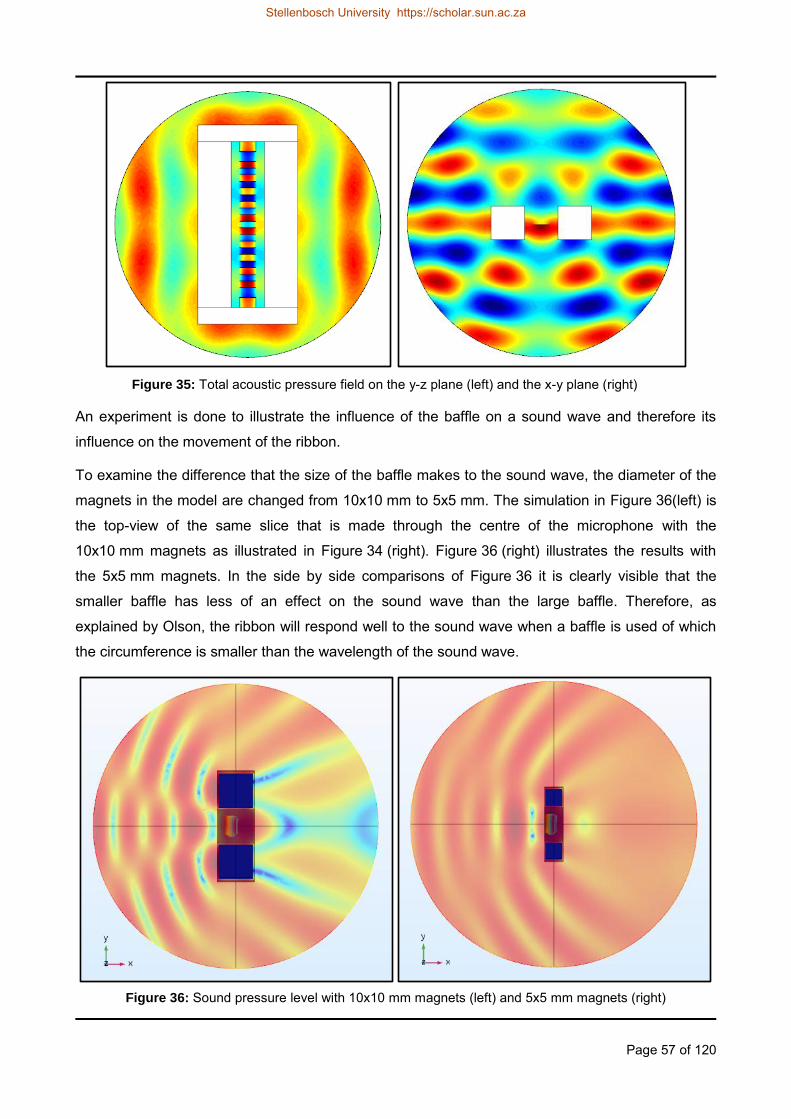
Page 57 of 120
Figure 35: Total acoustic pressure field on the y-z plane (left) and the x-y plane (right)
An experiment is done to illustrate the influence of the baffle on a sound wave and therefore its
influence on the movement of the ribbon.
To examine the difference that the size of the baffle makes to the sound wave, the diameter of the
magnets in the model are changed from 10x10 mm to 5x5 mm. The simulation in Figure 36(left) is
the top-view of the same slice that is made through the centre of the microphone with the
10x10 mm magnets as illustrated in Figure 34 (right). Figure 36 (right) illustrates the results with
the 5x5 mm magnets. In the side by side comparisons of Figure 36 it is clearly visible that the
smaller baffle has less of an effect on the sound wave than the large baffle. Therefore, as
explained by Olson, the ribbon will respond well to the sound wave when a baffle is used of which
the circumference is smaller than the wavelength of the sound wave.
Figure 36: Sound pressure level with 10x10 mm magnets (left) and 5x5 mm magnets (right)
Stellenbosch University https://scholar.sun.ac.za

Page 58 of 120
6.2.11 Impact of the Microphone Baffle on the Pressure Gradient
The ribbon microphone is a sound velocity microphone, also commonly known as pressure
gradient microphone. Figure 37 illustrates the pressure gradient across the ribbon of a microphone
on the x-z plane through the centre of the ribbon. It can be seen that the pressure gradient across
the ribbon of the microphone with 10x10 mm magnets is different from the pressure gradient
across the ribbon of the microphone with 5x5 mm magnets. This confirms once more that the size
of the baffle plays an important role at the upper frequencies where the wavelength of the sound
becomes comparable with the path length around the baffle.
Figure 37: Pressure gradient across the ribbon: 10x10 mm magnets (left) and 5x5 mm magnets (right)
6.3 Testing
No tests were conducted to illustrate the effects that are discussed in the modelling and simulation
paragraphs of the acoustics section, but the following test is advised for students that wish to put
the simulations into practice: Perform a test with the exact same setup (same sound equipment,
same acoustic environment, same microphone), but with two different thickness ribbons - 10um
and 20um. The test results will verify that the thicker (heavier) ribbon will have a lower amplitude
output signal and that resonance of the thicker ribbon is at a lower frequency.
6.4 Conclusion
Through modelling and simulation of the ribbon microphone and its acoustic environment, it can be
illustrated how physics concepts that are not included in the simple mathematical form will
influence its behaviour. Modelling and simulation can give students much more insight about
physics problems and its solutions than what can be accomplished by numerical methods alone.
Through simulation, the experiments in this section illustrate physics concepts like inertia,
mechanical structure, elasticity, pressure and waves. It also illustrates how statements in literature
can be verified through simulation; for instance that the path length around the microphone baffle
plays an important role in the frequency response of the microphone, as stated by Olson in his
patent for the first ribbon microphone.
Stellenbosch University https://scholar.sun.ac.za

Page 59 of 120
7 MECHANICS
The second physics area for which the ribbon microphone can be used as demonstration tool, is
that of mechanics. The mechanical response of a ribbon that is subjected to the effects of a sound
wave effectively illustrates the concept of resonance and deformation of mechanical structures.
The model may even be scaled to simulate the destructive results of resonance on large
mechanical structures like bridges.
This chapter presents 2 experiments which can be performed using a basic ribbon microphone.
A set of simulation experiments modelling different ribbon designs. The focus is on the
movement and deformation of the ribbon itself, with the object constituting the whole ribbon
in isolation from the microphone structure. The aim here is to illustrate how mechanical
design affects the dynamic movement and deformation of a thin foil in a wave and the
design impact on natural resonance.
A microphone experiment showing the effect of two ribbon designs. This real-world
experiment is presented here to demonstrate the credibility of simulations, but at the same
time to show the variances that can be expected when simulation models are incomplete.
7.1 Theory
Deformation of a ribbon in a sound wave will be illustrated by experiments in this chapter.
A random particle that is initially located at coordinate will follow a path during deformation that
can be described by
(21)
where is the spatial coordinate, is the material coordinate, and is the displacement.
The gradient of the displacement in a 3D system is
[
]
(22)
An infinitesimal line, can be mapped against its corresponding deformed line to give the
deformation gradient tensor
(23)
can be written in terms of the displacement gradient as
Stellenbosch University https://scholar.sun.ac.za
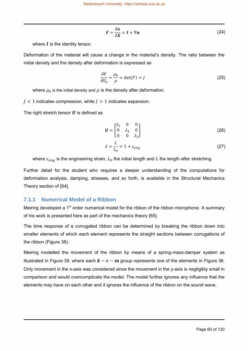
Page 60 of 120
(24)
where is the identity tensor.
Deformation of the material will cause a change in the material‟s density. The ratio between the
initial density and the density after deformation is expressed as
(25)
where is the initial density and is the density after deformation.
indicates compression, while indicates expansion.
The right stretch tensor is defined as
[
] (26)
(27)
where is the engineering strain, the initial length and the length after stretching.
Further detail for the student who requires a deeper understanding of the computations for
deformation analysis, damping, stresses, and so forth, is available in the Structural Mechanics
Theory section of [64].
7.1.1 Numerical Model of a Ribbon
Meiring developed a 1st order numerical model for the ribbon of the ribbon microphone. A summary
of his work is presented here as part of the mechanics theory [65].
The time response of a corrugated ribbon can be determined by breaking the ribbon down into
smaller elements of which each element represents the straight sections between corrugations of
the ribbon (Figure 38).
Meiring modelled the movement of the ribbon by means of a spring-mass-damper system as
illustrated in Figure 39, where each group represents one of the elements in Figure 38.
Only movement in the x-axis was considered since the movement in the y-axis is negligibly small in
comparison and would overcomplicate the model. The model further ignores any influence that the
elements may have on each other and it ignores the influence of the ribbon on the sound wave.
Stellenbosch University https://scholar.sun.ac.za

Page 61 of 120
Figure 38: Ribbon geometry for numeric model [65]
Figure 39: Spring-mass-damper model of a ribbon [65]
The basic form of a linear damped system is
(28)
where is the mass matrix, the damping matrix, the stiffness matrix and the vector of
displacement. is the matrix that contains the amplitude of the input force and the vector that
contains the trigonometric part of the input force as a function of time in seconds.
If and then (28) can be rewritten in terms of its displacement vector
( ) and velocity vector ( ) as
(29)
(30)
Stellenbosch University https://scholar.sun.ac.za

Page 62 of 120
Rewriting it as a single first-order equation yields
(31)
where *
+ (32)
*
+ (33)
*
+ (34)
with an identity matrix and an matrix of zeros.
The mass, damping and stiffness matrices in (28) represents
[
]
(35)
[
]
(36)
[
]
(37)
Stellenbosch University https://scholar.sun.ac.za
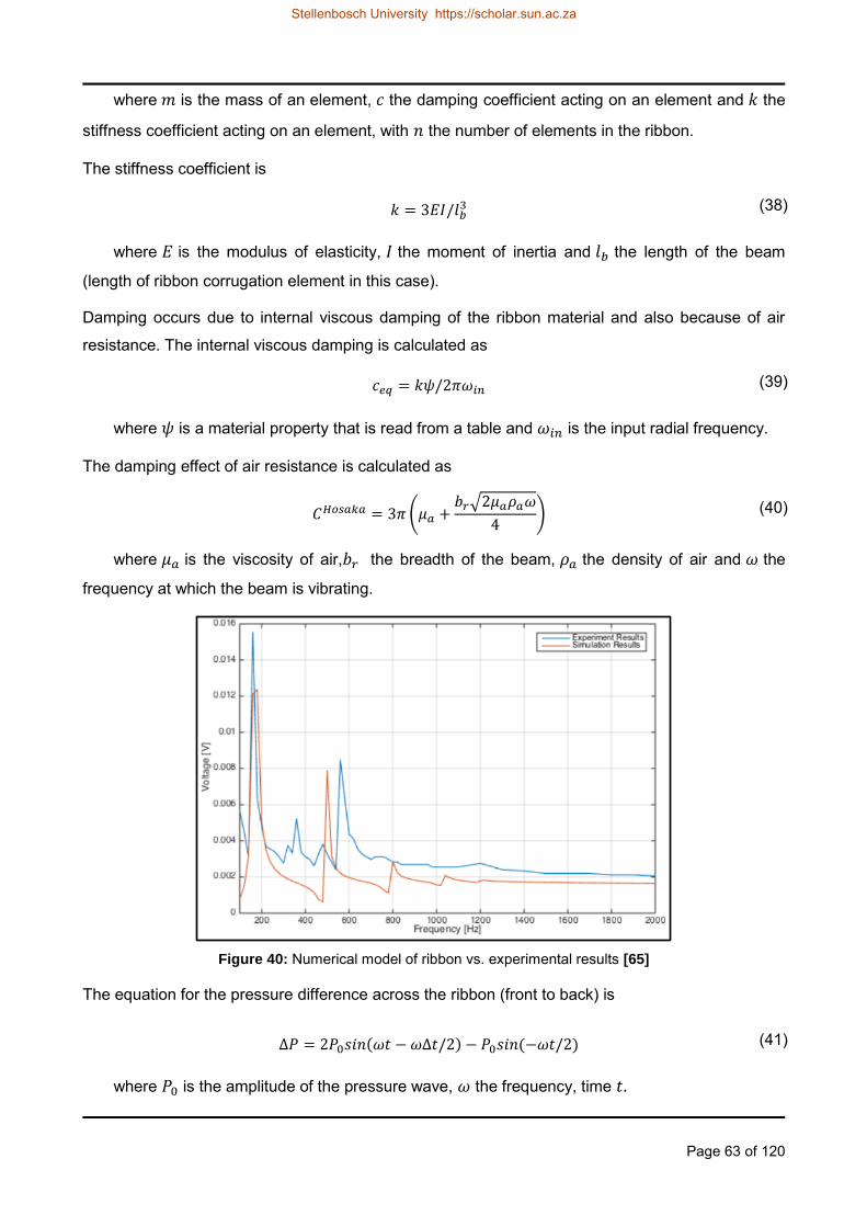
Page 63 of 120
where is the mass of an element, the damping coefficient acting on an element and the
stiffness coefficient acting on an element, with the number of elements in the ribbon.
The stiffness coefficient is
(38)
where is the modulus of elasticity, the moment of inertia and the length of the beam
(length of ribbon corrugation element in this case).
Damping occurs due to internal viscous damping of the ribbon material and also because of air
resistance. The internal viscous damping is calculated as
(39)
where is a material property that is read from a table and is the input radial frequency.
The damping effect of air resistance is calculated as
( √
) (40)
where is the viscosity of air, the breadth of the beam, the density of air and the
frequency at which the beam is vibrating.
Figure 40: Numerical model of ribbon vs. experimental results [65]
The equation for the pressure difference across the ribbon (front to back) is
(41)
where is the amplitude of the pressure wave, the frequency, time
Stellenbosch University https://scholar.sun.ac.za
Page 64 of 120
The phase lag between the front and the back of the ribbon is determined by
(42)
where is the path length around the microphone poles and is the speed of sound.
Meiring implemented all the equations in MATLAB® and determined the time response of the
system with the aid of the Runge-Kutta integration functions in MATLAB®.
From the velocity Meiring calculated the emf that is generated by the ribbon by means of Faraday‟s
law.
(43)
(44)
where is the emf, the change in magnetic flux, the magnetic flux density, the length
of the ribbon, the displacement and the time in which the displacement occurs.
The calculated emf was then verified experimentally. The results of the numerical model and the
experimental results by Meiring are shown in Figure 40.
7.2 Modelling and Simulation
After investigating the behaviour of a free floating disk in chapter 6 the model can now be
expanded to experiment with the ribbon itself. The next step is to simulate a ribbon without the
surrounding structure of the microphone baffle.
The ribbon model consists of a 40 mm long corrugated aluminium ribbon with a thickness of
10 µm, suspended in a three-dimensional volume. The ends of the ribbon are kept stationary by
adding a small element with extremely high mass at each end. The ribbon is placed inside a
sphere of limited dimension to keep the volume of the model small enough to compute a solution
within a reasonable time. The boundaries of the sphere are modelled in such a way that the sound
source outside of the sphere will enter the sphere without any reflections. Similarly, all sound
waves travelling inside the sphere are allowed to leave the sphere with minimal reflections from the
inside boundary of the sphere. The incident sound wave is modelled as a plane wave striking the
ribbon face-on, straight from the front.
7.2.1 Deformation and Resonance of the Ribbon
This experiment illustrates through simulation how the ribbon‟s mechanical structure influences its
resonance and how the ribbon deforms.
Stellenbosch University https://scholar.sun.ac.za

Page 65 of 120
Figure 41 illustrates the action of a fully corrugated ribbon in sound fields of 300 Hz and 3 kHz. At
3 kHz the largest section of the ribbon moves in unison, but at 300 Hz a standing wave is formed
along the ribbon. From the units on the colour scale it can be seen that the displacement of the
ribbon at 300 Hz is 100 times higher than the displacement at 3 kHz. Purely based on the
wavelengths of the two sound waves, the difference in displacement should be a factor of 10 only.
The difference by a factor of 100 indicates that the fully corrugated ribbon has a resonant
frequency at 300Hz.
Figure 41: Ribbon action in 300 Hz and 3 kHz sound waves
The displacement of a zigzag ribbon can be clearly displayed in a 3D model, but the displacement
amplitude cannot be easily plotted on a y-z graph for further analysis. It is possible to draw a cut-
line through the centre of the ribbon along the z-axis and plot various properties along the cut-line
on a graph. With the corrugations however, a straight line intersects the ribbon only at the points
where it pierces the ribbon. Therefore only a few dots are displayed on the graph. A projection of
the zigzag ribbon onto a flat surface will be a good option but such a solution is not available with
the simulation software. The displacement of the ribbon at 3 kHz is only a few hundred
nanometres, so there is no need for the ribbon to be corrugated along its whole length to provide
sufficient flexibility for this experiment. In an effort to circumvent the graphing problem the ribbon
design is changed from a completely corrugated ribbon to a flat ribbon with only two sections of
corrugation (one on each end) to give the ribbon enough flexibility, but with a long flat section that
can be plotted on a graph.
Stellenbosch University https://scholar.sun.ac.za

Page 66 of 120
Figure 42: Action of ribbon with two corrugations in 300 Hz and 3 kHz sound waves
Figure 43: Action of ribbon with one corrugation in 300 Hz and 3 kHz sound waves
Figure 44: Action of ribbon with no corrugation in 300 Hz and 3 kHz sound waves
Stellenbosch University https://scholar.sun.ac.za
Page 67 of 120
To evaluate the influence of the change in ribbon design, two other models are also introduced:
one with a single corrugation in the middle of the ribbon and another with no corrugations at all.
Figure 42 to Figure 44 illustrate how the shape of the ribbon influences its behaviour under the
stresses of sound waves at 300 Hz and 3 kHz. The graphs of the displacement along the cut-lines
are placed alongside the 3D results. The empty space that can be seen in the middle of the x-y
graph of Figure 43 is the corrugated piece of ribbon that does not fall on the cut-line. In Figure 42
the empty sections are not as noticeable because the corrugations are at the ends of the ribbon.
Only the ribbon with no corrugations (Figure 44) shows the displacement of the ribbon along its
total length.
It can be seen from the displacement differences between 300 Hz and 3 kHz that the ribbon with
two corrugations displays a large resonance at 300 Hz. The ribbon with one corrugation has a low
resonance at 300 Hz and the ribbon with no corrugation is not resonating at all. The ribbon with no
corrugation displays a standing wave in a similar fashion to that of a vibrating string. The ribbon
with one corrugation displays similar behaviour, but with slight twisting of the ribbon. The ribbon
with two corrugations twists and turns even more along its long straight section. The ribbons do not
twist at the corrugations, but only along the flat pieces. Although the ribbon without corrugation has
the longest straight section, it is too tightly strung to twist at these frequencies. With the movement
of Figure 41 in mind, it can be deduced that the corrugations along the length of the ribbon adds
mechanical stabilisation to the ribbon to prevent it from twisting and turning in the sound wave;
thereby preventing unwanted harmonics in the sound recording. The mean displacement along the
complete surface area of the ribbon is calculated by the simulation software. The displacement
results of the four ribbons at 3 kHz are 13.98 nm, 14.18 nm, 13.56 nm and 13.79 nm for the
ribbons with 10, 2, 1 and zero corrugations respectively. Although the physical behaviour of the
four ribbons is very different, the standard deviation for their displacement amplitudes is only
0.23 nm (i.e. less than 1.7% of the amplitudes) at 3 kHz. The calculated displacement results at
300 Hz (where two ribbons resonate) are 1.60 µm, 0.77 µm, 0.17 µm and 0.14 µm respectively.
It is clear that the corrugations in the ribbon play an important role in the stability of the ribbon.
Without regular corrugations the ribbon twists and turns (on a micro-scale) instead of moving in
parallel lines between the two magnets. It does not play much of a role in the displacement of the
ribbon at non-resonant frequencies however. Logarithmic plots of the displacement (averaged over
the total surface area of the ribbon) vs. frequency are shown in Figure 45 and Figure 46 for the
ribbons with ten corrugations and zero corrugations. The resolution of the graph is 20 Hz. The
resonance frequencies of the ribbons differ significantly, but the displacement values over the
60 Hz to 20 kHz range are of the same magnitude at the non-resonating frequencies. It could be
expected that the ribbon with ten corrugations will have a larger displacement value at lower
frequencies than the ribbon with no corrugations. However, the displacement is not governed by
Stellenbosch University https://scholar.sun.ac.za

Page 68 of 120
the flexibility of the ribbon alone, but also by the weight of the ribbon. More corrugations equal
more flexibility, but also more weight. Displacement that is gained by flexibility is lost again
because of additional weight. The ribbon may be compared to a vibrating string - the lighter the
string, the higher its natural frequency. The ribbon with many corrugations resembles a heavier,
more loosely strung string and the ribbon with no corrugations resembles a lighter, more tightly
strung string. Figure 45 and Figure 46 are good illustrations to demonstrate how the lower resonant
frequencies are more predominant with the corrugated ribbon (Figure 45) while the higher resonant
frequencies are more dominant with the non-corrugated ribbon (Figure 46).
Figure 45: Displacement vs. frequency for ribbon with ten corrugations
Figure 46: Displacement vs. frequency for ribbon with zero corrugations
This behaviour is in accord with Akino‟s statement in his gold plated ribbon patent that the ribbon is
folded in a zigzag form to lower the resonance frequency of the diaphragm [43]. The 300 Hz
frequency at which the ribbon in Figure 41 resonates can also be seen distinctly in the
Stellenbosch University https://scholar.sun.ac.za

Page 69 of 120
displacement graph of Figure 45. The ribbon with no corrugations shows no peak at 300 Hz. This
agrees with the results of the 3D visualization of the ribbon in Figure 44.
7.2.2 Velocity of the Ribbon
The amplitude of the emf that is generated by the ribbon is not determined by the extent of its
displacement, but rather by the velocity of the ribbon. Besides the length of the ribbon and the
intensity of the magnetic field, the velocity of the ribbon is the only other determining factor in the
magnitude of the generated emf in the following version of Faraday‟s law:
(45)
where is the emf, the velocity, the magnetic field, and the length of the conductor [66].
Figure 47 shows the velocity amplitude of the ribbon in the y-axis (averaged over the whole area of
the ribbon) plotted against frequency for the ribbon with ten corrugations. At 300 Hz the velocity is
3.67x10⁻³ m/s and at 3 kHz it is 0.32x10⁻³ m/s. For a magnetic field of 1 T and a ribbon length of
40 mm, the generated emf at 300 Hz is therefore 147 µV and at 3 kHz it is 13 µV. The emf
generated by the ribbon at its resonant frequencies is much higher than the emf at non-resonant
frequencies. This can cause unwanted harmonics in the sound recording.
Figure 47: Velocity amplitude vs. frequency for ribbon with ten corrugations
It can be seen in Figure 47 that the velocity of the ribbon increases slightly towards the higher
frequencies except for the self-resonance frequencies where there are large increases. The
difference in velocity at 100 Hz and 1 kHz is 5%. Between 1 kHz and 10 kHz the difference
increases to 17%. At the resonant frequencies the ribbon travels longer distances in the same time
period - therefore it travels at higher velocities.
Stellenbosch University https://scholar.sun.ac.za

Page 70 of 120
7.3 Testing
Simulations show that there is a difference in frequency response between a corrugated ribbon
and a straight ribbon. To support this finding a comparative test is conducted to determine whether
the differences are similar in a real-world setup.
7.3.1 Ribbon Corrugation
To perform the experiment for comparing different ribbons, a simple test setup is constructed with
the aid of a personal computer (PC). The test setup consists of the following:
A speaker set connected to the output of a PC‟s built-in sound card.
Ribbon microphone connected to the input of the PC‟s sound card.
REW software installed on the PC.
To perform the experiment, frequency scans are performed with two different ribbons – a
corrugated ribbon and a straight ribbon. Both ribbons are manufactured from 10 µm aluminium foil.
Although the test setup is not ideal, it is sufficient for this experiment because it is used for a
comparative test where only one of the variables is changed (the ribbon in this case) while the rest
of the variables remain fixed. Any deficiencies in the system that are visible with the corrugated
ribbon will have the exact same effect on the straight ribbon. The test is performed a few times with
the corrugated ribbon to confirm that the test results are consistently repeatable. Then the
corrugated ribbon is replaced with a straight ribbon and the same tests are repeated.
The result of the frequency scans of the two ribbons is shown in Figure 48. The dB scale in the
figure indicates the sound pressure level relative to the threshold of hearing. Smoothing of 1/12
octave is applied to the measurements to match the smoothing of Stanley‟s graph for the
hammered ribbon (Figure 49). The human ear perceives loudness with a smoothing effect between
1/3 and 1/6 octave. Due to its corrugations the corrugated ribbon is in effect longer, heavier and
more flexible than the straight ribbon. Therefore is has a lower resonance frequency. The result of
the real-world ribbon tests in Figure 48 confirms that the ribbon with corrugations has a better low
frequency response than the straight ribbon. The amplitude that falls towards the higher
frequencies in Figure 48 is the opposite of what is seen in the simulation results of Figure 47. The
difference in behaviour is attributed to the fact that the microphone baffle is not included in the
simulations. The influence of the baffle is demonstrated in paragraph 6.2.10. The simulated ribbons
in paragraph 7.2 are treated in isolation from the rest of the microphone and not all the effects of
the microphone design are taken into consideration. Furthermore, the physical ribbons are not
exact replicas of the simulated ribbons due to tooling and skill constraints when manufacturing the
DIY ribbons. Therefore resonance of the real-world ribbon will not be at the same frequency than
the simulated ribbon. The aim of the experiment is however to compare a corrugated ribbon to a
Stellenbosch University https://scholar.sun.ac.za

Page 71 of 120
straight ribbon to illustrate that the same effects that are observed with the simulated ribbons are
also seen with the laboratory tests. There is no indication in the REW documentation what the
reference level of dB-scale on the sound pressure level graph is. It is however not important for
comparative tests.
Figure 48: Frequency response of corrugated ribbon (blue) and straight ribbon (red)
7.3.2 Cold Working of an Aluminium Ribbon
No other tests were conducted to illustrate how the mechanical properties of the ribbon influence
the microphone‟s frequency response, but during the literature study a test by Stanley was found
that fits this category [67]. These tests were performed from a materials science point of view.
Stanley first looked at the use of alternative materials for the ribbon of the microphone. Nitinol, a
Nickel-Titanium alloy with excellent shape memory and super-elasticity properties would make the
ideal ribbon, but it is not available in micrometre range foils and its electrical resistivity is 30 times
higher than that of aluminium. Magnesium is lighter than aluminium, but a small piece of
magnesium foil is more expensive than a top-of-the-range ribbon microphone.
The next option was to treat the aluminium ribbon to change its physical properties. Stanley
conducted tests to determine whether cold working (hammering) of the ribbon would influence the
microphone‟s acoustic performance. Cold working changes the crystalline lattice structure of the
ribbon. He conducted the tests with an Apex 205 ribbon microphone. Only minor changes were
observed in the acoustic performance of the microphone when treating the ribbon by cold working
Stellenbosch University https://scholar.sun.ac.za
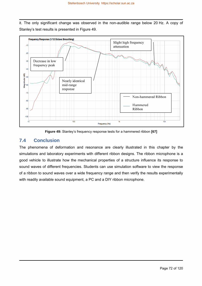
Page 72 of 120
it. The only significant change was observed in the non-audible range below 20 Hz. A copy of
Stanley‟s test results is presented in Figure 49.
Figure 49: Stanley‟s frequency response tests for a hammered ribbon [67]
7.4 Conclusion
The phenomena of deformation and resonance are clearly illustrated in this chapter by the
simulations and laboratory experiments with different ribbon designs. The ribbon microphone is a
good vehicle to illustrate how the mechanical properties of a structure influence its response to
sound waves of different frequencies. Students can use simulation software to view the response
of a ribbon to sound waves over a wide frequency range and then verify the results experimentally
with readily available sound equipment, a PC and a DIY ribbon microphone.
Stellenbosch University https://scholar.sun.ac.za

Page 73 of 120
8 MAGNETICS
The next physics area for which the ribbon microphone can be used as demonstration tool, is that
of magnetics. The propagation of a magnetic field in space and through obstacles, manipulation of
the magnetic field to meet the microphone‟s requirements and the effect of the physical structure of
the microphone, is visualised effectively through modelling and simulation.
The microphone requires high magnetic field strength inside the microphone, but low field strength
outside of the microphone. Modelling and simulation can be used to check new designs and design
parameters that are difficult to measure otherwise. A magnetic design can be characterised for
example, by taking hundreds of measurements with a Gauss meter and mapping it painstakingly
on a graph. For each new design all the measurements have to be performed all over again. A
more elegant solution is to create a simulation model and verify the simulation results with a limited
number of laboratory measurements.
This chapter presents 4 experiments which can be performed using the ribbon microphone.
Two simulation experiments modelling magnetic field lines and magnetic field strength.
Here the focus is on the magnetic aspect of the microphone assembly. The aim is to
illustrate mainly the impact of magnetic field manipulation.
Two laboratory experiments showing the magnetic field lines in the vicinity of the
microphone and the magnetic field strength in and around the microphone baffle. These are
of a modest nature and presented here to highlight the value of computer simulation when
expensive test equipment is not readily available, or experiments require cumbersome test
procedures.
8.1 Theory
8.1.1 Background
The term magnetic field describes the influence of two similar forces on its surroundings. The one
force is that of a magnet and the other, that of charges in motion. A magnetic field can be created
by a permanent magnet and it can also be created by an electric current.
The magnetic field is formed by force lines running from the north-pole to the south-pole of a
magnet. These force lines are called magnetic flux. It is denoted by the symbol and is measured
in the Système International d‟Unités (SI unit) weber (Wb). The term magnetic flux density refers to
the amount of flux per unit area perpendicular to the magnetic field.
(46)
where is the magnetic flux density, the magnetic flux and the area.
Stellenbosch University https://scholar.sun.ac.za
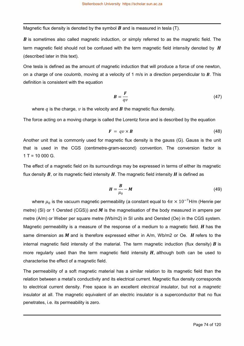
Page 74 of 120
Magnetic flux density is denoted by the symbol and is measured in tesla (T).
is sometimes also called magnetic induction, or simply referred to as the magnetic field. The
term magnetic field should not be confused with the term magnetic field intensity denoted by
(described later in this text).
One tesla is defined as the amount of magnetic induction that will produce a force of one newton,
on a charge of one coulomb, moving at a velocity of 1 m/s in a direction perpendicular to . This
definition is consistent with the equation
(47)
where is the charge, is the velocity and the magnetic flux density.
The force acting on a moving charge is called the Lorentz force and is described by the equation
(48)
Another unit that is commonly used for magnetic flux density is the gauss (G). Gauss is the unit
that is used in the CGS (centimetre-gram-second) convention. The conversion factor is
1 T = 10 000 G.
The effect of a magnetic field on its surroundings may be expressed in terms of either its magnetic
flux density , or its magnetic field intensity . The magnetic field intensity is defined as
(49)
where is the vacuum magnetic permeability (a constant equal to H/m (Henrie per
metre) (SI) or 1 Oersted (CGS)) and is the magnetisation of the body measured in ampere per
metre (A/m) or Weber per square metre (Wb/m2) in SI units and Oersted (Oe) in the CGS system.
Magnetic permeability is a measure of the response of a medium to a magnetic field. has the
same dimension as and is therefore expressed either in A/m, Wb/m2 or Oe. refers to the
internal magnetic field intensity of the material. The term magnetic induction (flux density) is
more regularly used than the term magnetic field intensity although both can be used to
characterise the effect of a magnetic field.
The permeability of a soft magnetic material has a similar relation to its magnetic field than the
relation between a metal‟s conductivity and its electrical current. Magnetic flux density corresponds
to electrical current density. Free space is an excellent electrical insulator, but not a magnetic
insulator at all. The magnetic equivalent of an electric insulator is a superconductor that no flux
penetrates, i.e. its permeability is zero.
Stellenbosch University https://scholar.sun.ac.za

Page 75 of 120
Magnetic materials may also be characterised by their polarisation (intensity of magnetisation),
which is defined as
(50)
The different measuring units in SI and CGS become quite confusing. Table 2 summarises the
different units and their conversion factors [68]. Literature dating back to the nineteen-sixties [69]
and earlier refer to the MKSA system instead of the SI system. MKSA stands for metre-kilogram-
second-ampere. For the remainder of this text only SI units will be used.
Table 2: CGS vs. SI units and its conversion factors
Unit Symbol CGS SI Conversion
Magnetic flux Gauss (G) Tesla (T) 10-4
Magnetic field intensity Oersted (Oe) A/m 103/4π
Magnetisation (magnetic dipole moment per unit volume)
erg/G/cm3 A/m 103
Magnetic permeability G/Oe H/m 4π x 10-7
Magnetic polarisation none Tesla None
8.1.2 Ferromagnetic Hysteresis Loop (Magnetisation Curve)
The ferromagnetic hysteresis loop is well described in [70] and [68]. A condensed version is
provided below.
The characteristics of a ferromagnetic material are determined by placing the material in an applied
external magnetic field and observing how the material‟s own magnetism changes as the external
field is increased, decreased or reversed. The results are plotted on a graph with the external
magnetic field on the x-axis and the material‟s own magnetic field on the y-axis. The
hysteresis loop is therefore also referred to as the M-H loop of the material (Figure 50).
and are both measured in ampere per metre (A/m). The unit of A/m is a relatively small unit
considering that the earth‟s magnetic field is approximately 50 A/m. The magnetic field of natural
magnetite (Fe3O4) is 480kA/m.
The four ideal types of magnetic material will behave as follow:
The ideal nonmagnetic material is not magnetic at all and it will not be magnetised by an
external field, no matter how large the external field. Its hysteresis curve is a straight
horizontal line on the x-axis ( ).
Stellenbosch University https://scholar.sun.ac.za

Page 76 of 120
The ideal hard magnetic material is permanently magnetised and its own magnetism will
not increase or decrease in the presence of an external field. Its hysteresis curve is a
straight horizontal line at a certain value of . No matter how large or how small that value
of is, it will not be changed by an external magnetic field of any magnitude.
The ideal soft magnetic material will be magnetised instantaneously by an external
magnetic field. Its hysteresis curve is a vertical line along the y-axis ( ).
The ideal diamagnetic material will be magnetised by an amount that changes linearly with
the external magnetic field. Its hysteresis curve is a straight line at a 45° angle.
Figure 50: Magnetisation hysteresis loop
The magnetisation of a sample that has never been magnetised before will follow the curve along
the red line (the virgin curve) in Figure 50 while is increased. If is increased only until reaching
point A on the curve and then decreased to zero again, the material will retain an amount of
magnetism of B. To demagnetise the sample again, an external field needs to be applied
with magnitude C in the opposite direction. If is increased beyond point A the sample will reach
magnetic saturation near point D. Beyond point D the magnetism of the sample will no longer
increase. As the external field is decreased, the magnetism of the sample will follow the green
curve. When the external field is removed ( ) a magnetisation strength of Mr will remain
in the sample. If a reverse field of increasing magnitude is applied externally, the sample‟s
magnetism will decrease along the green curve until reaches the value -HC. At this point the
sample will be demagnetised ( ). If the magnitude of the reverse field is further increased (
becomes more negative), the sample will become magnetised with opposite polarity. When point E
is reached the sample is saturated in the opposite direction. When the external field is increased
again, the sample‟s magnetism will follow the blue curve from point E to point D.
Stellenbosch University https://scholar.sun.ac.za

Page 77 of 120
Three points of particular interest are noted on the M-H curve:
MS – saturation or spontaneous magnetisation. This is the value of beyond which the
magnetisation of the material does not increase any further with an increase in the
externally applied .
Mr – remanence or retentivity. The amount of magnetisation that remains in the material
after the external magnetic field has been removed, i.e. the amount of magnetisation that
the material retains.
HC – coercivity. The intensity of an external field that is required to change the direction of
magnetisation of a material.
These parameters are used in calculations and simulation models for magnetic material. Another
quantity that is regularly used is the energy product of a magnet. is equal to the
area of the largest rectangle that can fit inside the second quadrant of the B-H curve. The B-H
curve is similar to the M-H curve, but the material‟s induction instead of its magnetisation is
plotted against .
Soft magnetic materials have narrow loops and lose their magnetisation as soon as the external
field is removed. The H-field penetrates soft magnetic materials only partially. Magnetic dipoles at
the surface of the sample are arranged in such a way that they shield the internal structure from
any external fields. Soft magnetic materials are fit for use as magnetic shields. Soft magnetic
materials have high permeability, low coercivity and small hysteresis losses and are therefore also
ideal for transformer cores and cores for motors and generators. Iron-cobalt-vanadium alloy
(Fe-C-V), iron-nickel alloy (Fe-Ni), amorphous alloy, silicon steel and ferrites are examples of soft
magnetic materials.
Hard magnetic materials have wide, square M-H curves. Once magnetised by applying an external
field, these materials will keep their magnetised state after the H-field has been removed. The
H-field penetrates hard magnetic materials completely. They are fit for use as permanent magnets.
Their high coercivity, high remanence and large hysteresis losses are the characteristics that make
these materials good permanent magnets. Neodymium-iron-boron alloy (NdFeB), samarium-cobalt
alloy (SmCo) and aluminium-nickel-cobalt alloy (AlNiCo) are examples of hard magnetic materials.
Permanent magnets gets demagnetised by vibration, opposing fields and high temperatures. The
temperature above which a magnet completely loses its magnetism is known as its Curie
temperature. At 1388 Kelvin, cobalt is the material with the highest Curie temperature. The
extremely strong NdFeB magnets that are most commonly in use today (N33 grade for example)
have a relatively low Curie temperature of 353 K (80°C). Special grades of these magnets (N33AH
for instance) may have Curie temperatures up to 513 K (240°C).
Stellenbosch University https://scholar.sun.ac.za

Page 78 of 120
The spontaneous magnetisation, remanence and coercivity of magnetic materials depend on many
factors. The rate at which is swept, its thermal history, the shape of the material, surface
roughness and microscopic defects are just a few of these factors. Physicists are trying to explain
the hysteresis loop. Materials scientists are figuring out how to improve it. Engineers are working
together to make the best use of it.
8.1.3 Ribbon Corrugation
Horng et al. states in their patent [47] that the ribbon is corrugated to lengthen the ribbon in order
for a larger part of the ribbon to cut the magnetic field, thereby enhancing the sensitivity. This is not
the case however. The emf is generated perpendicular to the movement of the ribbon and the
magnetic field. The corrugation changes the angle of the ribbon relative to the magnetic field lines
– thereby reducing the magnitude of the emf. The greatest electrical excitation is achieved when
the movement of the ribbon cuts the field lines perpendicularly. Any change in angle reduces the
amplitude of the generated emf, thereby counteracting the gain in ribbon length. The simplified
equation for the generated emf is
(51)
where is the emf, the velocity, the magnetic field, and the length of the conductor [66].
This equation is however only true for perpendicular movement. The complete equation for other
angles of movement is
(52)
where is the angle between the direction of movement and the magnetic field.
For a straight ribbon that is 50 mm long, vibrating at an average speed of 1.25 um/s, in a magnetic
field of 1.2 T, the generated emf will be
If the ribbon is fully corrugated with corrugations at 45° to the length of the ribbon, then the ribbon
length will increase to 70.710678 mm. The generated emf will be
The calculations show that no sensitivity is gained by corrugating the ribbon. Calculations for
corrugations at other angles produce the same results.
The ribbon is in fact corrugated because the corrugations add flexibility to the ribbon for its forward-
backward movement while simultaneously providing mechanical stability to the ribbon in the other
directions. The corrugations have a large influence on the frequency response of the microphone
and the resonant frequencies of the ribbon as shown earlier in paragraph 7.
Stellenbosch University https://scholar.sun.ac.za

Page 79 of 120
8.2 Modelling and Simulation
Simulation results of the magnetic field lines in (and around) the ribbon microphone of 5.2.1.1 are
illustrated here and manipulation of the field lines with yokes of different metals is demonstrated.
8.2.1 Direction of Field Lines
The magnetic field needs to cut the ribbon perpendicular to its direction of motion to generate the
highest emf. Figure 51 illustrates the magnetic field lines between the two magnets of the
microphone and also in the area surrounding the magnets. It can be seen from the size of the
arrows that the flux density is at its highest between the two magnets and inside the magnets
themselves. Figure 52 provides a graph of the magnetic flux density along the x-axis (cutting
through the centre of both magnets) and a graph of the flux density along the y-axis (cutting
through the open space between the two magnets where the ribbon will move). Figure 53
illustrates with a different visualisation effect how the pole piece design influences the flux density
and the flow of the magnetic field lines by comparing a design with square-bar magnets to a design
with round-bar magnets. The slice is made on the x-y plane in the same position as for Figure 51.
Figure 51: Magnetic field lines – perspective view and top view of slice on x-y plane
Figure 52: Magnetic flux density on z-x plane (left) and y-z plane (right)
Stellenbosch University https://scholar.sun.ac.za
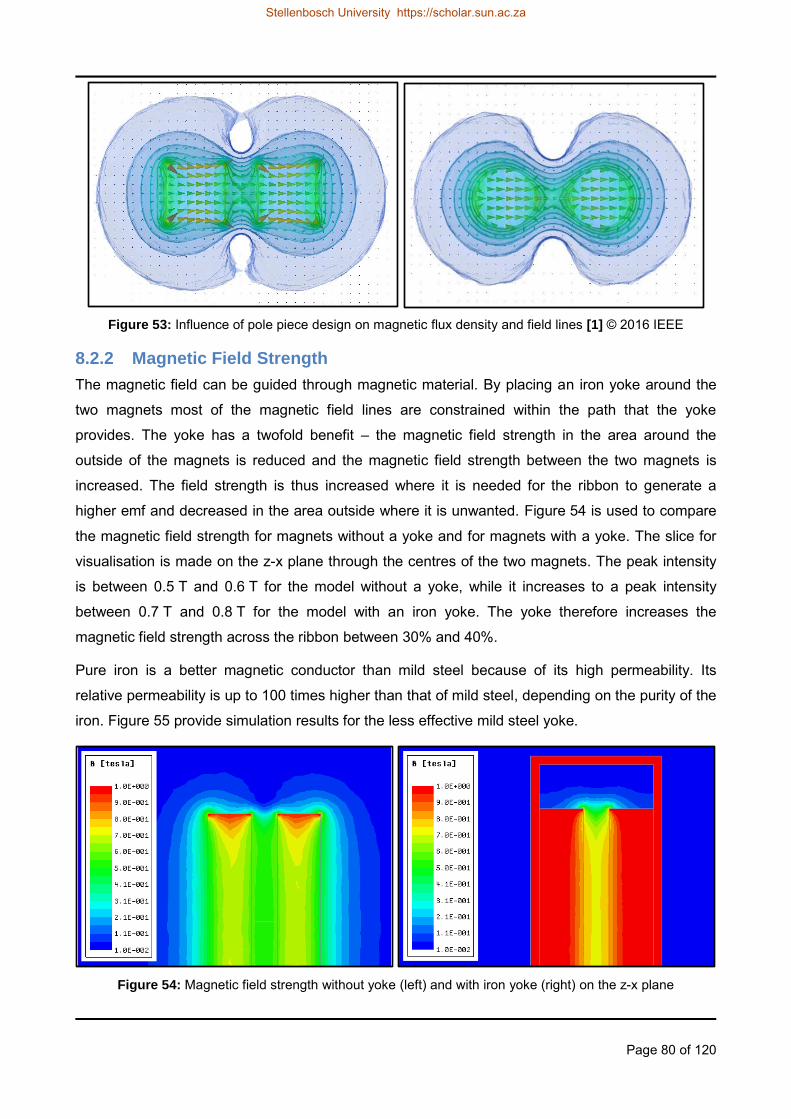
Page 80 of 120
Figure 53: Influence of pole piece design on magnetic flux density and field lines [1] © 2016 IEEE
8.2.2 Magnetic Field Strength
The magnetic field can be guided through magnetic material. By placing an iron yoke around the
two magnets most of the magnetic field lines are constrained within the path that the yoke
provides. The yoke has a twofold benefit – the magnetic field strength in the area around the
outside of the magnets is reduced and the magnetic field strength between the two magnets is
increased. The field strength is thus increased where it is needed for the ribbon to generate a
higher emf and decreased in the area outside where it is unwanted. Figure 54 is used to compare
the magnetic field strength for magnets without a yoke and for magnets with a yoke. The slice for
visualisation is made on the z-x plane through the centres of the two magnets. The peak intensity
is between 0.5 T and 0.6 T for the model without a yoke, while it increases to a peak intensity
between 0.7 T and 0.8 T for the model with an iron yoke. The yoke therefore increases the
magnetic field strength across the ribbon between 30% and 40%.
Pure iron is a better magnetic conductor than mild steel because of its high permeability. Its
relative permeability is up to 100 times higher than that of mild steel, depending on the purity of the
iron. Figure 55 provide simulation results for the less effective mild steel yoke.
Figure 54: Magnetic field strength without yoke (left) and with iron yoke (right) on the z-x plane
Stellenbosch University https://scholar.sun.ac.za

Page 81 of 120
Figure 55: Magnetic field strength with mild steel yoke
The yoke is not only beneficial for the magnetic field strength, but it also serves as a convenient
structure to hold the magnets in place. Because the magnets are so much closer to the yoke than
to each other, the magnets are attracted more to the yoke then to each other and remains stuck to
the yoke instead of snapping together.
8.3 Testing
Two experiments are performed to illustrate the magnetic effects of the microphone assembly. One
of the tests is used to demonstrate the direction of the magnetic field lines, and the other test is
used to measure the strength of the magnetic field.
8.3.1 Magnetic Field Lines
The magnetic field lines are checked with a handheld magnetic search pole consisting of a small
bar magnet on a gimbal (Figure 56). The gimbal allows the bar magnet to swivel freely in any
direction in order to align itself with the magnetic field lines.
Figure 56: Magnetic search pole
A simple check with this device (Figure 57) confirms that the magnetic field lines run in the same
pattern that the simulation shows in Figure 51. The red coloured side of the search pole is its north
pole and the blue side is its south pole.
A magnetic compass (Figure 58) can also be used, but the movement of the compass is restricted
to a single plane. Although most compass needles have a red north pole, there is not a clear
standard in this regard. The north pole of the compass in Figure 58 is the white side of the needle.
Stellenbosch University https://scholar.sun.ac.za

Page 82 of 120
Figure 57: Magnetic field lines indicated by search pole
Figure 58: Magnetic field lines indicated by magnetic compass
Stellenbosch University https://scholar.sun.ac.za

Page 83 of 120
8.3.2 Magnetic Field Strength
Gauss meters that measure magnetic field strength are not only expensive, but are also difficult to
find. Only a limited number of laboratories are equipped with a Gauss meter.
A simple custom made device is constructed in order to measure the field strength. The device
consists of a Honeywell SS49E linear hall-effect sensor IC wired to a battery and a multimeter
(Figure 60). The output from the SS49E varies linearly in proportion to the magnetic field strength
According to its datasheet the typical output is 1.4 mV per Gauss. Using the conversion factor in
Table 2 gives 1.4 mV per 1x10⁻⁴ Tesla, or 14 V per Tesla. The SS49E‟s limited supply voltage only
allows a magnetic range of ±1 000 Gauss (±0.1 T). Its range is well below the maximum field
strength of the simulation, but it is still useful in the areas of weaker magnetic field strength.
The output of the SS49E for zero Gauss is a voltage halfway between its supply lines. For a 3 V
supply the zero Gauss reading will be 1.5 V and for a 6 V supply it will be 3 V for example. The
device is also sensitive to the direction of the field lines. When the field lines are running perfectly
parallel to the device then it measures no magnetic field strength. When the field lines run
perpendicular to the device as indicated in Figure 59 the output voltage will increase or decrease
depending on the direction of the magnetic field. The voltage will increase for field lines running
south to north through the device and decrease for field lines running north to south through the
device.
A couple of spot-checks with this measuring device, as shown in Figure 61, confirms that the
magnetic field on the outside of the soft-iron yoke is weaker than the magnetic field between the
two magnets inside the yoke. These checks agree with the simulation results of Figure 55.
Figure 59: SS49E field line direction
Stellenbosch University https://scholar.sun.ac.za
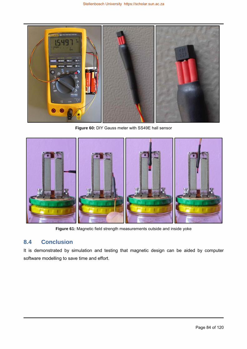
Page 84 of 120
Figure 60: DIY Gauss meter with SS49E hall sensor
Figure 61: Magnetic field strength measurements outside and inside yoke
8.4 Conclusion
It is demonstrated by simulation and testing that magnetic design can be aided by computer
software modelling to save time and effort.
Stellenbosch University https://scholar.sun.ac.za

Page 85 of 120
9 ELECTROMAGNETICS
The last of the physics areas for which the ribbon microphone is used as demonstration tool, is that
of electromagnetics.
The complete microphone system can be used to include circuit and system concepts in the
teaching model. The two techniques by which useful signal levels can be obtained from a ribbon
microphone, namely via a transformer or an amplifier, both offer excellent opportunities for
teaching circuit concepts through experimentation and simulation. In the case of the transformer,
concepts like transformation ratios, impedance matching and the frequency dependence of real-
world transformers can be illustrated, while for amplifiers concepts like noise, input impedance and
bandwidth can be shown.
This chapter presents 4 experiments which can be performed using transformers and electronic
amplifiers with the ribbon microphone.
A simulation experiment modelling two audio transformers of differing size, winding ratio
and impedance. Here the focus is on the components that complete the microphone
system. The aim of the simulation is to illustrate the impact that winding turns and core
material have on transformer frequency response and to show transformer behaviour under
various loads.
Laboratory experiment with transformers showing the effects of impedance matching. The
aim of this practical experiment is to illustrate the importance of impedance matching.
Laboratory experiment with electronic amplifiers. The aim of this experiment is to
demonstrate the effect of an RC filter and noise handling with electronic amplifiers.
Laboratory experiment with the microphone. The aim of this experiment is to provide a test
environment consisting of a complete microphone system, to compare the performance of
transformers and electronic amplifiers on a system level.
9.1 Theory
The ribbon microphone is a classic example of electromagnetic induction. By means of a micro-
meter-thin aluminium ribbon that is suspended in a magnetic field, it converts sound energy into
electric energy. The audio transformer that is used with the microphone is an excellent example of
low frequency electromagnetic coupling.
9.1.1 Faraday’s Law
Electromagnetic analysis is handled on a macroscopic level during simulation by solving Maxwell‟s
equations within a set of boundary conditions. The four Maxwell equations that form the basis for
fundamental electromagnetism calculations are Ampère‟s law, Faraday‟s law, Gauss‟ law for
Stellenbosch University https://scholar.sun.ac.za

Page 86 of 120
electric fields and Gauss‟ law for magnetic fields. For the purpose of this chapter, only Faraday‟s
law is required. The differential form and the integral form of the equation are provided in Table 3.
Table 3: Faraday‟s law
Differential Form Integral Form
∮
∮
∮
∫
Faraday‟s law describes the relationship between an electric field and a changing magnetic field.
Changing magnetic flux through a conducting surface induces an emf across the conductor. The
symbols that are used in Faraday‟s law are listed in Table 4. For further reading and a concise
introduction to Maxwell‟s equations see [71].
Table 4: Symbols used in Faraday‟s law
Symbol SI unit Quantity name or description SI unit, non-abbreviated
V/m
N/C Electric Field Intensity
Volt per metre
Newton per Coulomb
T
Magnetic Flux Density
Magnetic Induction
Magnetic Field
Tesla
9.1.2 Transformers
The amplitude of the emf generated in the vibrating ribbon of the microphone is too low for
transmission through a long cable without being drowned by ambient electromagnetic interference.
The signal-to-noise-ratio of the microphone output can be improved by amplifying its voltage by
means of a step-up transformer close to the microphone ribbon. The transformer is also vital for
impedance matching with amplifiers and recording equipment on the other end of the cable.
The ideal transformer is a device that will step an AC voltage up or down in the same ratio over all
frequencies and independent of any source or load impedance. With practical transformers there
are however many factors that influence the performance of the transformer. These influences are
so severe that transformers have to be designed specifically for different applications. A summary
of the factors that influence the characteristics of a transformer is provided in this paragraph [72].
Stellenbosch University https://scholar.sun.ac.za

Page 87 of 120
9.1.2.1 Turns-ratio
The turns-ratio of a transformer causes the following transformations in an ideal transformer:
Voltage transformation is directly proportional to the turns-ratio.
Current transformation is inversely proportional to the turns-ratio.
Impedance transformation is proportional to the square of the turns-ratio.
The turns-ratio of a transformer is the most basic part of its function, but it can also be the most
misleading parameter on the transformer‟s datasheet. The immediate thought of a transformer with
a 1:2 turns-ratio is that it will double the voltage. It is however only true for a limited frequency
range and is also dependent on the impedances of the circuits that are connected to the windings.
9.1.2.2 Magnetising Current and Core Loss
The current in the primary winding of the transformer sets up the mutual flux in the core and it
balances the demagnetising effect of the load current in the secondary winding. The net
magnetomotive force is related to the reluctance in the transformer core according to the equation
(53)
where is the number of turns in the primary and secondary windings, is the current in
these windings, is the magnetic flux in the core and is the reluctance of the core.
There is a magnetising inductance associated with the reluctance of the core and the core has
finite permeability. The flux in the core is established by the instantaneous magnetising current
which is determined by the magnetic properties of the core. When the core goes into saturation the
distorted magnetising current contains odd harmonics. The magnetising current increases rapidly
as the transformer go further into saturation. Hysteresis is a cause of power loss in the core at high
frequencies. Eddy current losses add to the hysteresis loss in high power applications.
9.1.2.3 Winding Resistance
Besides the DC resistances of the wires that are used for the transformer windings, there is also an
AC resistance component due to the internal flux of the wires (conductors). The AC resistance can
by approximated as
[ ( )
( ) ]
(54)
where is the skin depth of the conductor and is the radius of the conductor.
AC losses in the form of skin effect and proximity effects have to be taken into account for high-
frequency operation of transformers.
Stellenbosch University https://scholar.sun.ac.za

Page 88 of 120
9.1.2.4 Magnetic Leakage
Ideally the same magnetic flux will link the primary and secondary windings of the transformer
(mutual flux). In reality however, there is always an amount of flux limited to one winding that does
not link all the windings (leakage flux). Because of leaking flux there is not 100% power transfer
between windings and power is wasted.
9.1.2.5 General Transformer Equations
High-frequency loss in transformers is not of much concern in the audible frequency range.
Therefore the equations to follow are more than adequate for the purpose of the thesis.
Voltage Equation: The impressed voltage ( ) on a winding is related to the rate of change of flux
density according to Faraday‟s law.
(55)
where is the number of winding turns, the effective cross-sectional area of the magnetic
core and the flux density.
Power Equation: The total VA rating of a transformer can be related to its physical, electrical and
magnetic properties according to the equation
∑ (56)
where is the voltage waveform factor, the frequency, the maximum flux density,
the current density, the core stacking factor, the window utilisation factor and the product
of the window winding area and cross-sectional area.
Winding Loss: The total resistive loss in the windings of the transformer is
(57)
where is the electrical resistivity and the winding volume.
Core Loss: The total core loss under sinusoidal excitation can be calculated with the general
Steinmetz equation
(58)
where is the time-average core loss per unit volume and the peak value of the flux
density at a sinusoidal frequency . , and are constants that can be found in the
manufacturer‟s datasheet.
Stellenbosch University https://scholar.sun.ac.za

Page 89 of 120
9.1.3 Resistance of the Ribbon
The resistance of the ribbon does not feature in Faraday‟s law (45) because emf is the potential
difference when no current is flowing from the source [73]. The resistance of the ribbon only
becomes a factor when an external path is created for a current to flow. When an external current
path exists, the current in the circuit will be limited by the combined resistance of the load and the
ribbon. The current flowing in the circuit can be calculated as:
(59)
where is the current, the emf, the resistance of the external circuit (load), and the
resistance of the ribbon itself.
The amplitude of the signal across the load is:
(60)
where is the voltage across the load, the current, and the resistance of the load.
Substituting with (59) yields:
(61)
The amplitude of the emf that is seen across a load will therefore increase when lowering the
resistance of the ribbon. The material that the ribbon is made of as well as its thickness and width,
will determine the resistance of the ribbon. The following trade-offs have to be considered for the
design of the ribbon:
A thicker ribbon will have lower electrical resistance but it will present higher mechanical
resistance to the sound wave because of the additional weight.
A wider ribbon will have lower resistance and will present a larger area for the sound wave
to impose on, but once again it will be heavier.
Lower resistance of the ribbon will result in higher amplitudes, but also in higher currents
that will increase the effect of Eddy currents on the ribbon. The Eddy currents act like a
magnetic brake on the ribbon and adversely affect its velocity, thereby limiting the
generated emf.
There is only a limited amount of energy present in a sound wave that has to overcome both the
mechanical inertia of the ribbon and the effect of the Eddy currents. The design of the ribbon is
therefore a balancing act between electrical resistance, physical area and weight. If the external
load has relatively low impedance, like a transformer for instance, the resistance of the ribbon
plays an important role, but if the external circuit has very high impedance (like an instrumentation
amplifier) then the resistance of the ribbon has very little effect on the signal amplitude.
Stellenbosch University https://scholar.sun.ac.za
Page 90 of 120
9.2 Modelling and Simulation
9.2.1 Transformer
Transformers that are used to step up the voltage of a ribbon microphone are good examples of
low frequency electromagnetic coupling. The transformer is not only used to step up the output
voltage of the microphone, but also for impedance matching with the audio equipment that is
connected to the microphone.
Two transformers from different manufacturers are chosen for simulation and testing.
The RMX-1 transformer from EDCOR is chosen because it is a transformer that is
specifically designed for ribbon microphones.
The SP-48 transformer is chosen because it is a miniature MIL-SPEC audio transformer
that will fit neatly inside a microphone enclosure.
Little of the information that is necessary for modelling these transformers is available from the
datasheets. Some of the unknown parameters can be measured on the physical RMX-1 model
without any damage, but the SP-48 transformer is completely encapsulated in epoxy. The same
parameters can therefore not be measured on the SP-48.
COMSOL® provides a physics interface that gives the user full control over the core and coil
geometries and the materials of the transformer model. ANSYS® PEmag on the other hand
provides the user with comprehensive lists of commercial parts (cores, bobbins, wires and winding
topologies) that can be used to design a transformer from standardised commercially available
components. The RMX-1 and SP-48 are specialised transformers that do not contain the standard
parts found in PEmag. ANSYS® also has an Electronic Transformer Kit (ETK) for Maxwell, but the
ETK is intended for ferrite core transformers in the 100 kHz range and not for the low frequency
range of the audio band. The coil design toolkit for Maxwell can be used to calculate coil resistance
and number of turns that fit on a bobbin. The toolkit accepts coil dimensions in millimetre, but the
wire thickness must be entered in American Wire Gauge (AWG). Many conversion tables are
available on the internet, but most of these tables have the thinnest wire size of 30 AWG or
32 AWG. Only a few tables indicate wire sizes as thin as 40 AWG. For thinner wires a conversion
calculation is necessary. The equation to convert from metric wire diameter to AWG is
(
) (62)
where is the AWG number and the wire diameter in millimetre [74].
Stellenbosch University https://scholar.sun.ac.za

Page 91 of 120
9.2.1.1 Simulation models
The simulation models for the transformers in the experiments here are based on the E-core
transformer example that is supplied by COMSOL® as a tutorial. The basic example is taken as a
starting point and then customised to suit the RMX-1 and SP-48 transformers.
The following factors have a distinct influence on the simulation models and will be discussed in
more detail later in this section:
Number of turns on the primary winding
Source impedance
Load
Core material
9.2.1.2 EDCOR RMX-1 transformer
The parameters that are used to model the RMX-1 transformer are listed in Table 5.
Table 5: RMX-1 transformer parameters
Parameter Magnitude Source
Turns-ratio 1:37 Datasheet
DC Resistance Primary : 0.4 Ohm
Secondary : 87 Ohm Datasheet
Core material Super Q 80 Nickel (80%) Datasheet
E-core dimensions
Outer : 25.5 mm x 19.0 mm x 6.65 mm
Inner : 18.5 mm x 12.5 mm
Centre : 7.0 mm x 12.5 mm
Measured
Wire diameter
Primary : 380 µm, double wound.
Secondary : 120 µm, single wound.
Wire thickness includes insulation. Heavy insulation on
primary, light insulation on secondary.
Measured
Bobbin
Outer diameter (including shielding foil) : 17.2 mm
Inner diameter : 9.8 mm
Winding height : 11 mm
Measured
Number of turns Primary : 38
Secondary : 1395 Calculated
Stellenbosch University https://scholar.sun.ac.za

Page 92 of 120
The Maxwell® 3D Coil Design Toolkit from ANSYS® is used to calculate the number of turns on the
RMX-1 coil windings. The RMX-1 does not consist of a simple inner and outer winding. The
primary winding has two wires - one wire winding around the outside of the coil and the other wire
somewhere in-between the windings of the secondary coil. The parameters for the inner diameter
of the bobbin, the coil height and the wire thickness for the secondary coil are first entered in the
toolkit. Then the outer diameter of the coil is adjusted until the coil resistance equals the datasheet
value. This method yields an answer of 1395 turns on the secondary winding. There are then 38
turns on the primary winding according to the turns-ratio of the transformer.
The parameter entry window of Maxwell® is shown in Figure 62 and the geometry of the coil is
illustrated in Figure 63.
Figure 62: Maxwell® coil design toolkit – parameter entry
Figure 63: Maxwell® coil design toolkit – coil geometry
Stellenbosch University https://scholar.sun.ac.za

Page 93 of 120
Once the necessary parameters of the transformer are determined with the aid of ANSYS®
Maxwell®, a model for the transformer is created in COMSOL®. The mesh of the transformer
model and a simulation of the magnetic flux density are illustrated in Figure 64. Students can
create animations with the simulation software to visualise how the flux density and the current
changes as a function of time, to gain an even better understanding of the functioning of
transformers.
Figure 64: Mesh of RMX-1 model (geometry in mm) and magnetic flux density (Tesla)
To demonstrate the influence that the number of turns of the primary winding has on the
transformer‟s performance, a set of simulations is run with different numbers of turns. Simulations
are done for frequencies ranging from 10 Hz to 30 kHz and for the number of turns on the primary
winding ranging from 5 turns to 140 turns. The simulation results are exported from COMSOL® and
then processed in Microsoft Excel for display in graphical format. The results for a 10 mV (RMS)
sinusoidal excitation of the primary winding with 2kΩ and 3 kΩ loads are presented in Figure 65
and Figure 66. The load on the output of the transformer also plays a role in the outcome of the
simulations.
It is clear from the simulations that a low number of turns have a negative effect on the output of
the transformer. A higher number of turns causes the output voltage to increase but if the number
of turns is increased beyond a certain point, then the output voltage starts to decrease at higher
frequencies. The reason is that the inductance increases with the increasing number of turns. The
point where the graphs of all the frequencies intersect is a good choice for the number of turns to
use. For the simulations that are presented here the ideal number of turns is somewhere between
35 and 41, depending on the load conditions. The earlier calculation of 38 turns fits well within this
range.
Stellenbosch University https://scholar.sun.ac.za

Page 94 of 120
Figure 65: Number of turns on primary winding vs. output voltage (2kΩ load)
Figure 66: Number of turns on primary winding vs. output voltage (3kΩ load)
In COMSOL® the source of the test signal has zero impedance and there are no resistive losses
between the source and the transformer. In a laboratory test setup however, the source has a fixed
impedance and there is considerable resistance between the source and the transformer due to
the connections and wires to the test equipment. A series resistance of 0.3 Ω between the signal
source and the transformer is added for this reason during simulation. To illustrate the influence
that the source impedance has on the results, a set of simulations are run where the source
impedance is changed from 0.1 Ω to 6.4 Ω. The results for a 2 kΩ load are shown in Figure 67 and
for a simulation with a 3 kΩ load in Figure 68. With a source impedance somewhere between
0.2 Ω to 0.4 Ω the transformer should have a relatively flat frequency response depending on the
load. The selection of a 0.3 Ω series resistance for the simulation is therefore an acceptable
choice.
Stellenbosch University https://scholar.sun.ac.za

Page 95 of 120
Figure 67: Influence of source impedance on output voltage (2 kΩ load)
Figure 68: Influence of source impedance on output voltage (3 kΩ load)
These results are for simulations that are performed with a mu-metal transformer core. Nickel
alloys that contain high percentages of nickel (around 79%) have high initial permeability and high
maximum permeability, with very low hysteresis losses. The addition of molybdenum or copper
further promotes specific magnetic properties. MolyPermalloys (typical 80% Ni, 4 to 5% Mo,
balance Fe) and mu-metals (typical 77% Ni, 5% Cu, 2% Cr, balance Fe) are popular high
permeability alloys [75]. The magnetic characteristics of these alloys make them ideal for
transformer cores. The RMX-1 datasheet specifies Super Q 80 Nickel (80%) as the core material.
The closest match in the simulation software‟s materials library is “Nickel Steel Mumetal 80% Ni”.
The HB curve for this material is included in the library. Figure 69 shows a comparison between
the simulation results with a mu-metal core and a soft iron core. This comparison illustrates that the
magnetic characteristic (given by the HB curve) is an important factor in the transformer design. Of
Stellenbosch University https://scholar.sun.ac.za
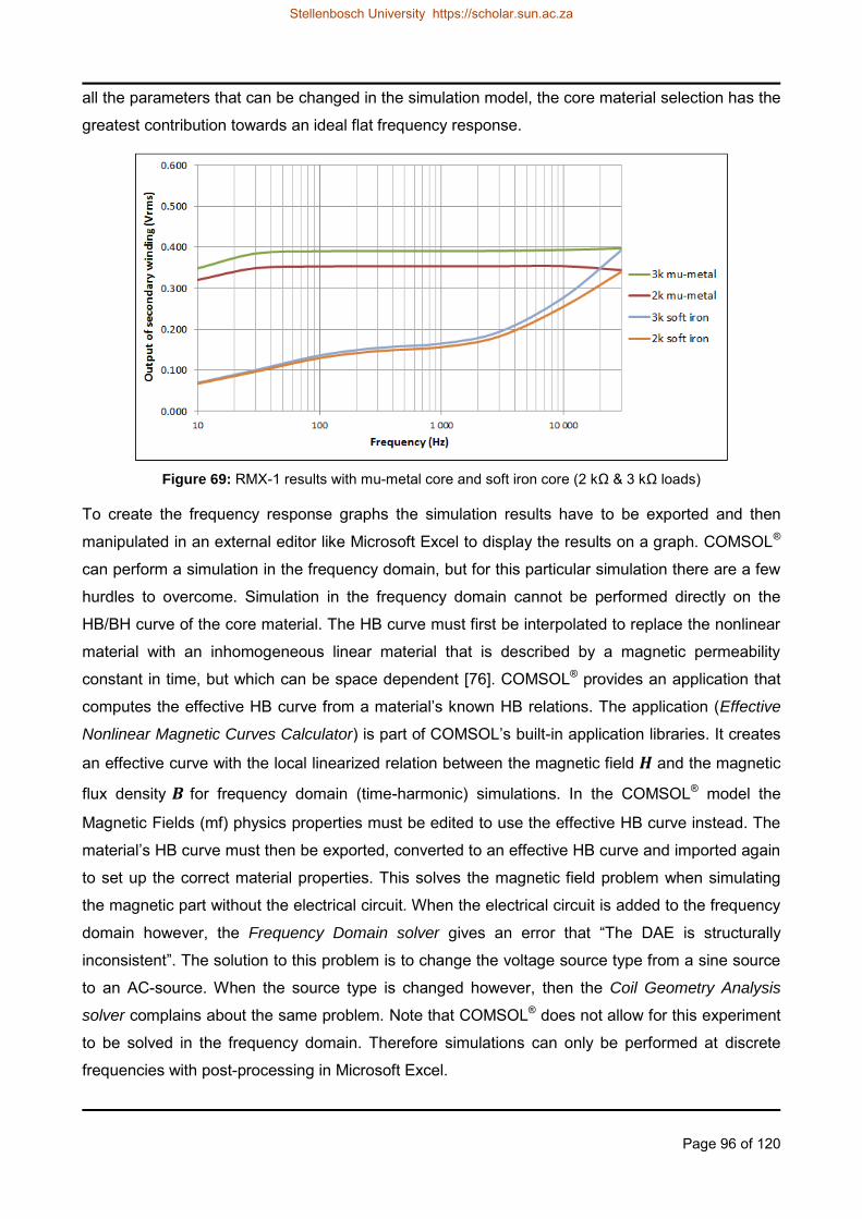
Page 96 of 120
all the parameters that can be changed in the simulation model, the core material selection has the
greatest contribution towards an ideal flat frequency response.
Figure 69: RMX-1 results with mu-metal core and soft iron core (2 kΩ & 3 kΩ loads)
To create the frequency response graphs the simulation results have to be exported and then
manipulated in an external editor like Microsoft Excel to display the results on a graph. COMSOL®
can perform a simulation in the frequency domain, but for this particular simulation there are a few
hurdles to overcome. Simulation in the frequency domain cannot be performed directly on the
HB/BH curve of the core material. The HB curve must first be interpolated to replace the nonlinear
material with an inhomogeneous linear material that is described by a magnetic permeability
constant in time, but which can be space dependent [76]. COMSOL® provides an application that
computes the effective HB curve from a material‟s known HB relations. The application (Effective
Nonlinear Magnetic Curves Calculator) is part of COMSOL‟s built-in application libraries. It creates
an effective curve with the local linearized relation between the magnetic field and the magnetic
flux density for frequency domain (time-harmonic) simulations. In the COMSOL® model the
Magnetic Fields (mf) physics properties must be edited to use the effective HB curve instead. The
material‟s HB curve must then be exported, converted to an effective HB curve and imported again
to set up the correct material properties. This solves the magnetic field problem when simulating
the magnetic part without the electrical circuit. When the electrical circuit is added to the frequency
domain however, the Frequency Domain solver gives an error that “The DAE is structurally
inconsistent”. The solution to this problem is to change the voltage source type from a sine source
to an AC-source. When the source type is changed however, then the Coil Geometry Analysis
solver complains about the same problem. Note that COMSOL® does not allow for this experiment
to be solved in the frequency domain. Therefore simulations can only be performed at discrete
frequencies with post-processing in Microsoft Excel.
Stellenbosch University https://scholar.sun.ac.za

Page 97 of 120
A cheaper Shinhom T25 transformer is available from China as a replacement for the more
expensive RMX-1 from America. According to the T25 specification sheet, the RMX-1‟s frequency
response is as depicted in Figure 70. This graph is for an unknown load.
Figure 70: Frequency response of RMX-1 according to its competitor of the T25
9.2.1.3 Triad SP-48 transformer
The SP-48 transformer is not analysed and simulated in as much detail as the RMX-1 transformer.
The SP-48 is completely encapsulated in epoxy and it is therefore not possible to measure the wire
thicknesses of the windings. The construction of a Triad SP-13 transformer that is similar to the
SP-48 is shown in Figure 71. The core dimensions of the SP-13 are the same as the SP-48, but
the wire thickness is different.
Figure 71: Cross section of Triad SP-13 transformer
A simulation model of the SP-48 is created with the same number of primary windings and core
material than the RMX-1, but with different turns-ratio, smaller core and higher winding resistance.
The parameters of the SP-48 transformer are listed in Table 6 alongside the parameters of the
RMX-1 transformer. Figure 72 shows a comparison between the simulation results of the SP-48
and RMX-1 transformers.
Stellenbosch University https://scholar.sun.ac.za

Page 98 of 120
Table 6: SP-48 and RMX-1 transformer parameters
Parameter SP-48 RMX-1
Turns-ratio 1:25 1:37
DC Resistance Primary : 2.9 Ohm
Secondary : 796 Ohm
Primary : 0.4 Ohm
Secondary : 87 Ohm
Core material Unknown Super Q 80 Nickel (80%)
E-core dimensions
Outer : 9.6 mm x 6.4 mm x 4.0 mm
Inner : 7.4 mm x 4.2 mm
Centre : 2.4 mm x 4.2 mm
Outer : 25.5 mm x 19 mm x 6.65 mm
Inner : 18.5 mm x 12.5 mm
Centre : 7.0 mm x 12.5 mm
Wire diameter Primary : Unknown
Secondary : Unknown
Primary : 380 µm, double wound.
Secondary : 120 µm, single wound.
Bobbin
Outer diameter : 4.6 mm
Inner diameter : 3.0 mm
Winding height : 3.4 mm
Outer diameter : 17.2 mm
Inner diameter : 9.8 mm
Winding height : 11 mm
Number of turns Primary : 38
Secondary : 950
Primary : 38
Secondary : 1395
Figure 72: SP-48 simulation results vs. RMX-1 simulation results (2 kΩ & 3 kΩ loads)
9.2.2 Microphone
No simulations demonstrating the emf generated by the microphone are provided here. Simulation
of the induced emf in the ribbon is not simple. The ribbon can be simulated by using the single-turn
coil model and the Magnetic Fields (mf) Study in COMSOL®. To compute the emf of the ribbon, the
Stellenbosch University https://scholar.sun.ac.za

Page 99 of 120
two ends of the ribbon must touch the external walls of the air domain surrounding the conductor.
When the geometry of the model is changed so that the ribbon touches the boundary walls
however, multiple other problems arise and the model causes mutually conflicting conditions.
9.3 Testing
9.3.1 Transformer
The emf generated by the ribbon microphone is extremely low – in the order of a few hundred
microvolt and less. To work at voltages this low is extremely difficult because of ambient
electromagnetic noise and the sensitivity of the test equipment that is required. Therefore the
laboratory tests are performed with signals in the millivolt range rather than the microvolt range.
The RMX-1 and SP-48 transformers Figure 73 are used in the experiments.
Figure 73: RMX-1 and SP-48 transformers
9.3.1.1 Manual Measurements
To verify the simulated results in section 9.2.1 a selection of discrete measurements are taken with
a simple test setup. The Wavetek function generator and the Fluke multimeter are used for this
experiment. The minimum output voltage of the function generator is 650 mV AC. To reduce the
test voltage into the millivolt range a resistor divider network is used to reduce the output voltage of
the function generator. A diagram of the test setup is provided in Figure 74. The output of the
function generator is adjusted until 10 mV (RMS) is measured across the 1.1 ohm resistor while a
10 kΩ load is connected to the secondary side of the transformer. The voltages are then measured
across the load on the secondary winding of the transformer for different loads and frequencies.
The test results are provided in Table 7 for the RMX-1 transformer and in Table 8 for the SP-48
transformer. See Figure 75 and Figure 76 for graphical representations of these measurements
and comparisons of measured versus simulated results.
Stellenbosch University https://scholar.sun.ac.za

Page 100 of 120
Figure 74: Test setup for manual transformer measurements
Table 7: RMX-1 measurements
Freq RMX-1 output (mV RMS) at loads of
(Hz) 1k2 2k 3k 10k Open circuit
10 128 162 188 240 268
30 140 184 217 290 338
100 144 189 224 305 360
300 145 191 227 310 368
1 000 146 192 229 314 372
3 000 147 194 231 318 378
10 000 148 195 234 322 383
30 000 145 193 232 324 386
Table 8: SP-48 measurements
Freq SP-48 output (mV RMS) at loads of
(Hz) 1k2 2k 3k 10k Open circuit
10 50 65 77 103 118
30 65 89 110 161 200
100 70 97 121 185 238
300 71 98 123 190 248
1 000 71 99 124 192 250
3 000 71 99 125 194 253
10 000 69 98 124 195 257
30 000 55 83 109 194 269
Stellenbosch University https://scholar.sun.ac.za

Page 101 of 120
Figure 75: RMX-1 simulated results (sim) vs. measured results (meas)
Figure 76: SP-48 simulated results (sim) vs. measured results (meas)
9.3.1.2 Automated Measurements
The number of measurements done by hand is limited to a few discrete frequencies. A wide range
of frequencies can be covered in a short period of time by automated testing. Every student that
owns a personal computer (PC) with a sound card can perform automated tests with little effort.
With a similar resistor divider network as used in 9.3.1.1 an automated test is set up with the aid of
a PC and software. John Mulcahy‟s REW software is used for this purpose. The test setup is
shown in Figure 77.
First an automated loop-back calibration test is performed to compensate for the sound card‟s own
non-linearity. The output of the sound card is connected directly to the input of the sound card for
calibration. Thereafter, the divider network and transformer with 10 kΩ load are connected. The
output level of the sound card is adjusted until 10 mV (RMS) is measured with a multimeter across
Stellenbosch University https://scholar.sun.ac.za
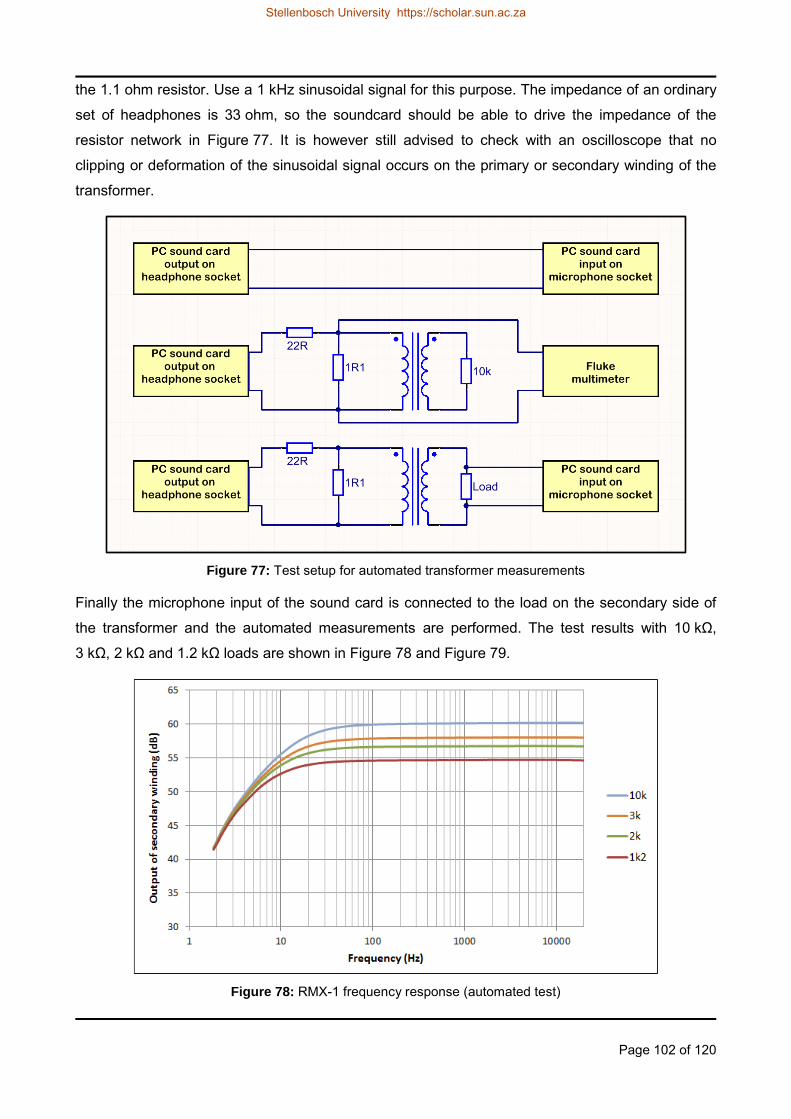
Page 102 of 120
the 1.1 ohm resistor. Use a 1 kHz sinusoidal signal for this purpose. The impedance of an ordinary
set of headphones is 33 ohm, so the soundcard should be able to drive the impedance of the
resistor network in Figure 77. It is however still advised to check with an oscilloscope that no
clipping or deformation of the sinusoidal signal occurs on the primary or secondary winding of the
transformer.
Figure 77: Test setup for automated transformer measurements
Finally the microphone input of the sound card is connected to the load on the secondary side of
the transformer and the automated measurements are performed. The test results with 10 kΩ,
3 kΩ, 2 kΩ and 1.2 kΩ loads are shown in Figure 78 and Figure 79.
Figure 78: RMX-1 frequency response (automated test)
Stellenbosch University https://scholar.sun.ac.za

Page 103 of 120
Figure 79: SP-48 frequency response (automated test)
With the soundcard‟s input connected to the 1.1 ohm resistor in the same position as the
multimeter, in order to check the signal level on the primary winding of the transformer, the
soundcard reads 33.4 dB while a 10 kΩ load is connected. The RMX-1 provides therefore a
26.6 dB gain (i.e. 21 times gain factor) instead of the ideal 37 times gain (31.4 dB) as per it turns-
ratio. The SP-48 provides a gain of 21.1 dB (i.e. 11 times gain factor). It can be seen that even with
a high impedance load such as 10 kΩ, the voltage gain provided by a transformer is substantially
less than the ideal gain based on its turns-ratio.
9.3.1.3 Impedance Matching
The output impedance of a ribbon microphone is typically less than one ohm and the input
impedance of an amplifier can range anywhere between 1 kΩ and 10 kΩ depending on the model.
A transformer may be used to match the impedance between the microphone and the amplifier of
a sound system. With the wide range of amplifiers that are available a single transformer will
unfortunately not always match the impedance of the amplifier. The laboratory test results and the
simulated results discussed earlier illustrate how source and load impedances have an influence
on the signal transfer from source to load. The loads that are chosen represent two selectable
impedances of the Focusrite Scarlett 2i2 computer audio interface and two selectable impedances
of the Buzzaudio MA-2.2 professional microphone amplifier.
A complete table of impedances versus frequencies for the RMX-1 and SP-48 secondary windings
is provided in Table 9. The impedances on the secondary winding are measured while a 1.1 Ω
resistor remains connected to the primary winding.
Stellenbosch University https://scholar.sun.ac.za

Page 104 of 120
Table 9: Impedances of secondary transformer winding at different frequencies
Freq (Hz) DC 10 30 100 300 1 000 3 000 10 000 30 000
RMX-1 impedance (Ω)
88 1 620 1 758 1 826 1 858 1 889 1 945 2 065 2 249
SP-48 impedance (Ω)
787 1 898 2 825 2 994 3 058 3 096 3 215 3 802 7 463
The maximum power transfer theorem states that maximum power is transferred from a source to
a load when the impedances of the source and the load are equal [72]. A transformer may be used
to match the impedance between a source and its load. Reflected impedance is commonly used in
electronic circuits to achieve maximum power transfer. To test the validity of this theorem in the
current test setup the test results in Table 7 and Table 8 are used to calculate the power transfer to
each load. The results of the power calculations that are presented in Table 10 and Table 11
support the maximum power theorem. These results are good illustrations that most power is
transferred to the load that match the output impedance of the transformer. The same can be
illustrated for the input of the transformer, but it is more difficult to perform measurements on the
low voltage signals of the primary winding. This experiment illustrates how the electromagnetic
properties of a transformer can be utilized to minimize energy losses when transferring energy
from a low impedance source to a high impedance load.
Table 10: RMX-1 power transfer (µW) to different loads
Freq (Hz) 10 30 100 300 1 000 3 000 10 000 30 000
1.2 kΩ load 13.65 16.33 17.28 17.52 17.76 18.01 18.25 17.52
2 kΩ load 13.12 16.93 17.86 18.24 18.43 18.82 19.01 18.62
3 kΩ load 11.78 15.70 16.73 17.18 17.48 17.79 18.25 17.94
10 kΩ load 5.76 8.41 9.30 9.61 9.86 10.11 10.37 10.50
Table 11: SP-48 power transfer (µW) to different loads
Freq (Hz) 10 30 100 300 1 000 3 000 10 000 30 000
1.2 kΩ load 2.08 3.52 4.08 4.20 4.20 4.20 3.97 2.52
2 kΩ load 2.11 3.96 4.70 4.80 4.90 4.90 4.80 3.44
3 kΩ load 1.98 4.03 4.88 5.04 5.13 5.21 5.13 3.96
10 kΩ load 1.06 2.59 3.42 3.61 3.69 3.76 3.80 3.76
9.3.2 Electronic Amplifier
The same tests that are performed with the two transformers are also performed with two
electronic amplifiers.
Stellenbosch University https://scholar.sun.ac.za

Page 105 of 120
The first amplifier is the AD8231 instrumentation amplifier from Analog Devices. An instrumentation
amplifier is chosen because of its high common mode rejection ratio (100-120 dB). The AD8231 in
particular is chosen for its low voltage operation (±1.5V to ±2.5V), low input offset (4-15 µV) and
the fact that it has binary selectable gains of 1 to 128.The schematic for the AD8231 electronic
amplifier circuit is provided in Figure 80.
The second amplifier is the INA103 instrumentation amplifier from Texas Instruments. The INA103
is chosen because it is a high fidelity amplifier, specifically designed for low noise operation. The
schematic for the INA103 electronic amplifier circuit is shown in Figure 81. The gain resistor (47 Ω)
on the INA103 is selected to match the highest gain (128) of the AD8231.
Figure 80: AD8231 amplifier schematic
Figure 81: INA103 amplifier schematic
Stellenbosch University https://scholar.sun.ac.za

Page 106 of 120
The same automated test setup (Figure 77) that is used for the transformers is also used with the
amplifiers.
The AD8231 is tested at different gains, since the gain can be easily changed with just a few
switches. The test results are displayed in Figure 82. The gain of the AD8231 is independent of the
load. Load tests that are done with loads ranging from 1.2 kΩ to 10 kΩ all give identical results
than Figure 82 across all gains. With a gain of one on the AD8231, the sound card reads 29.6 dB
for a 1 kHz sine wave. The detailed data of Figure 82 shows a level of 59.9 dB at 1 kHz for a gain
selection of 32 on the AD8231. The effective gain is then 30.3 dB. This is very close to the
theoretical gain of 30 dB. See Table 12 for a quick conversion between gain as a multiplication
factor and gain in dB.
Figure 82: AD8231 amplifier gain test
To illustrate the influence of the RC-filter on the input of the amplifier the 100 kΩ resistors on the
AD8231‟s inputs are changed to 10 kΩ. The result is a filter that suppresses the lower frequencies.
This is clearly illustrated in Figure 83.
An electronic amplifier has the advantage that it adds energy to the signal during amplification.
That energy is taken from the circuit‟s power supply.
Stellenbosch University https://scholar.sun.ac.za

Page 107 of 120
Figure 83: AD8231 amplifier gain test with high pass filter
The electronic amplifier does not only add energy to the signal, but it also adds noise in the
process. Each of the components in the amplifier adds noise into the circuit and this noise is
amplified together with the microphone signal through all the consecutive stages of the amplifier.
The noise is clearly audible as a “hiss” when the signal is further amplified by the final stage
amplifier. For this reason there are high fidelity amplifiers available that are specifically designed
for low noise operation. The INA103 instrumentation amplifier is one example of such an amplifier.
Listening tests conducted with the INA103 confirm that the noise level of this low noise amplifier is
orders of magnitude lower than the AD8231. The noise level of the INA103 is comparable with that
of a transformer. The frequency response of the IN103 versus the AD8231 at a gain of 128 is given
in Figure 84.
Figure 84: INA103 vs. AD8231 frequency response at gain of 128
Stellenbosch University https://scholar.sun.ac.za

Page 108 of 120
Table 12: Voltage gain multiplication factor to voltage gain in dB
Gain multiplier Gain in dB
128 42
100 40
64 36
37 31
32 30
25 28
16 24
8 18
9.3.3 Microphone
To conclude the hardware tests the ribbon microphone is connected to each transformer and
amplifier for a frequency sweep.
The test setup consists of the following:
Ribbon microphone
RMX-1 and SP-48 transformers
AD8231 and INA103 amplifier circuits
Dell Optiplex 9020 PC
Logitech S-220 speaker set
REW software
Figure 85: Test setup with ribbon microphone and RMX-1 transformer
Stellenbosch University https://scholar.sun.ac.za

Page 109 of 120
Figure 86: Ribbon microphone and SP-48 transformer
The frequency sweeps with the two transformers are shown in Figure 87. The frequency responses
are very similar, only with the RMX-1 providing a higher gain than the SP-48.
The frequency dip between 50 Hz and 90 Hz is not a function of the transformers or the
microphone. It is a problem with the transition between the subwoofer and the main speakers of
the S-220 set. This is a frequency band that is poorly covered by both speakers.
Figure 87: Microphone frequency response with RMX-1 (blue) and SP-48 (red)
The RMX-1 is compared to the AD8231 amplifier with a gain setting of 32 in Figure 88. Once again
the frequency responses are very similar. Although the gain of the AD8231 is lower than the 1:37
turns-ratio of the RMX-1, the AD8231 provides a higher gain because it is not influenced like the
transformer by the load impedance.
Stellenbosch University https://scholar.sun.ac.za

Page 110 of 120
Figure 88: Microphone frequency response with RMX-1 (blue) and AD8321 (green)
In Figure 89 the AD8231 results are shown for gains of 32 and of 128. In the last illustration
(Figure 90) the results of the AD8231 and INA103 are illustrated with gains of 128. Although it
cannot be seen on the frequency response graphs, the INA103 has much less background noise
than the AD8231 when listening to the microphone. The noise level of the INA103 is almost as low
as the two transformers, but its gain is much higher, making it ideal as a ribbon microphone
amplifier.
Figure 89: Microphone with AD8231 amplifier at gains of 32 and 128
Stellenbosch University https://scholar.sun.ac.za

Page 111 of 120
Figure 90: Microphone with AD8231 (green) and INA103 (purple)
9.4 Conclusion
One of the benefits of simulations is that parameters can be changed that are not always possible
with the hardware at hand. The core material of the transformer is such an example. Although it
cannot be verified with an experiment, the simulation exercises show that the choice of material for
the transformer core plays a more important role in its performance than any of the other
parameters that can be changed.
The following comparisons can be drawn between transformers and electronic amplifiers according
to the tests results in 9.3:
• Transformers work well for impedance matching, but the output signal amplitude is load
dependent. It is however a passive component that requires no external power.
• Electronic amplifiers work well for impedance matching and the amplitude of the output
signal is not load dependent. It is however an active component that requires external
power.
• A properly shielded transformer adds almost no audible noise to the signal, but most
electronic amplifiers, even when properly shielded from ambient electrostatic noise, adds a
substantial amount of audible noise to the signal. Only specially designed low noise
amplifiers can match the noise levels of a transformer.
The impedance difference of a transformer between a DC signal and an AC signal clearly
illustrates the importance of frequency when it comes to impedance matching. DC tests are much
simpler to perform and the mathematics is less complicated than AC tests, but it can be totally
Stellenbosch University https://scholar.sun.ac.za
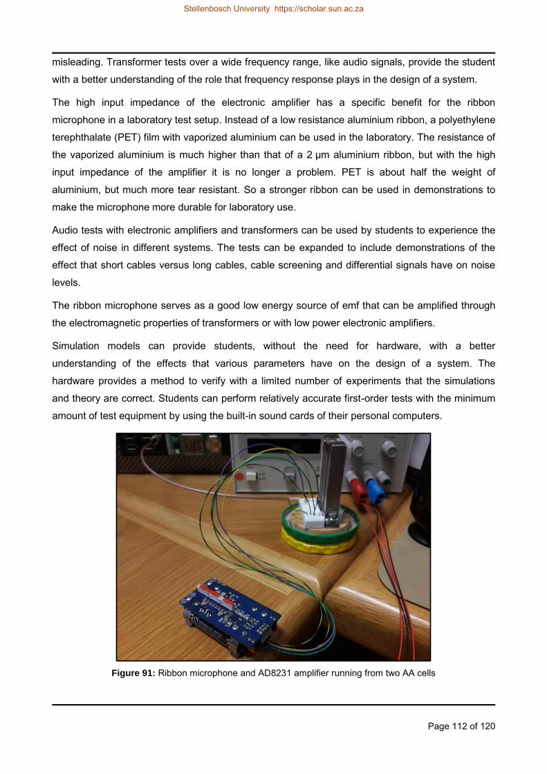
Page 112 of 120
misleading. Transformer tests over a wide frequency range, like audio signals, provide the student
with a better understanding of the role that frequency response plays in the design of a system.
The high input impedance of the electronic amplifier has a specific benefit for the ribbon
microphone in a laboratory test setup. Instead of a low resistance aluminium ribbon, a polyethylene
terephthalate (PET) film with vaporized aluminium can be used in the laboratory. The resistance of
the vaporized aluminium is much higher than that of a 2 µm aluminium ribbon, but with the high
input impedance of the amplifier it is no longer a problem. PET is about half the weight of
aluminium, but much more tear resistant. So a stronger ribbon can be used in demonstrations to
make the microphone more durable for laboratory use.
Audio tests with electronic amplifiers and transformers can be used by students to experience the
effect of noise in different systems. The tests can be expanded to include demonstrations of the
effect that short cables versus long cables, cable screening and differential signals have on noise
levels.
The ribbon microphone serves as a good low energy source of emf that can be amplified through
the electromagnetic properties of transformers or with low power electronic amplifiers.
Simulation models can provide students, without the need for hardware, with a better
understanding of the effects that various parameters have on the design of a system. The
hardware provides a method to verify with a limited number of experiments that the simulations
and theory are correct. Students can perform relatively accurate first-order tests with the minimum
amount of test equipment by using the built-in sound cards of their personal computers.
Figure 91: Ribbon microphone and AD8231 amplifier running from two AA cells
Stellenbosch University https://scholar.sun.ac.za

Page 113 of 120
10 A FINAL WORD
Considering the minute movement of an aluminium ribbon in a sound wave, it is a truly amazing
accomplishment that someone could, more than eighty years ago, detect and amplify the voltage
generated by this tiny movement in a magnetic field.
Of all the theory that was mastered and the discoveries that were made during the work for this
thesis, none was as valuable as witnessing first-hand how many consistent, seemingly insignificant
efforts, over a long period of time, come together to accomplish a task that seemed so
insurmountable at times.
Stellenbosch University https://scholar.sun.ac.za

Page 114 of 120
11 REFERENCES
[1] M. van Wyk and P. Meyer, “The Ribbon Microphone - An Educational Aid,” in 3rd International
Conference on Advances in Computational Tools for Engineering Applications (ACTEA), Zouk
Mosbeh, Lebanon, 2016.
[2] National Academy of Engineering, “Engineering in K-12 Education,” National Academic Press,
Washington D.C., 2009.
[3] National Research Council, “Engineering Graduate Education and Research,” NATIONAL
ACADEMY PRESS, Washington, D.C., 1985.
[4] National Academies of Science, Engineering & Medicine, “Undergraduate Research
Experiences for STEM Students: Successes, Challenges and Opportunities,” National
Academies Press, Washington, D.C., 2017.
[5] National Research Council, “Engineering Undergraduate Education,” National Academy Press,
Washington, D.C, 1986.
[6] B. H. Ferri, A. A. Ferri, D. M. Majerich and A. G. Madden, “Effects of In-class Hands-On
Laboratories in a Large Enrollment, Multiple Section Blended Linear Circuits Course,”
Advances in Eingineerin Education, pp. 1-27, 2016.
[7] National Research Council, “Improving Indicators of the Quality of Science and Mathematics
Education in Grades K-12,” National Academy press, Washington, D.C., 1988.
[8] N. Savage, R. Birch and E. Noussi, “Motivation of engineering students in higher education,”
Engineering Education, pp. 39-46, 2011.
[9] National Research Council, “Transforming Undergraduate Education in Science, Mathematics,
Engineering, and Technology,” National Academy Press, Washington, D.C., 1999.
[10] National Research Council, “Discipline-Based Education Research,” National Academies
Press, Washington, D.C., 2012.
[11] National Research Council, “Education and learning to think,” Nationl Academy Press,
Washington, D.C, 1987.
Stellenbosch University https://scholar.sun.ac.za

Page 115 of 120
[12] National Research Council, “From Analysis to Action: Undergraduate Education in Science,
Mathematics, Engineering and Technology,” National Academy Press, Washington, D.C.,
1996.
[13] L. D. Feisel and A. J. Rosa, “The Role of the Laboratory in Undergraduate Engineering
Education,” Journal of Engineering Education, pp. 121-130, 2005.
[14] X. Liu, “Effects of Combined Hands-on Laboratory and Computer Modeling on Student
Learning of Gas Laws: A Quasi-Experimental Study,” Journal of Science Education and
Technology, pp. 89-100, 2006.
[15] D. Heise, “Asserting the inherent benefits of hands-on laboratory projects vs. computer
simulations,” in Consortium for Computing Sciences in Colleges (CCSC), Central Plains
Conference, 2006.
[16] B. Taylor, P. Eastwood and B. Jones, “Development of a Low-cost, Portable Hardware
Platform to Support Hands-on Learning in the Teaching of Control and Systems Theory,”
Engineering Education, pp. 62-73, 2014.
[17] S. Lee, M. C. Harrison and C. L. Robinson, “Engineering students‟ knowledge of mechanics
upon arrival: Expectation and reality,” Engineering Education, pp. 32-38, 2006.
[18] F. W. Sears, M. W. Zemansky and H. D. Young, University Physics, USA: Addison-Wesley,
1982.
[19] R. T. Beyer, Sounds of Our Times, New York: Springer, 1999.
[20] P. White, Basic Microphones, London: Sanctuary Publishing Limited, 1999.
[21] J. Eargle, The Microphone Book, Burlington: Focal Press, 2005.
[22] G. Ballou, J. Ciaudelli and V. Schmitt, Handbook for Sound Engineers, Burlington: Focal
Press, 2008.
[23] H. F. Olson, “Apparatus for converting sound vibrations into electrical variations”. US Patent
1885001, 31 March 1931.
[24] J. F. Schneider, Bay Area Radio (Images of America), Charleston: Arcadia Publishing, 2012.
Stellenbosch University https://scholar.sun.ac.za

Page 116 of 120
[25] W. Dooley, “Evolution of an icon,” Technology, pp. 58-60, September 2008.
[26] D. E. Royer and R. T. Perrotta, “Ribbon-microphone transducer”. US Patent 2006/0078135, 8
October 2004.
[27] R. Cloud and S. Sank, “Ribbon microphone with rounded magnet motor assembly, backwave
chamber, and phantom powered JFET circuit”. US Patent 8433090, 9 October 2010.
[28] H. F. Olson, “Apparatus for converting sound vibrations into electrical variations”. United
States Patent 1885001, 25 October 1932.
[29] H. F. Olson and J. Weinberger, “Sound Pick-up Device”. US Patent 19115, 4 April 1933.
[30] L. J. Anderson, “Electroacoustical apparatus”. US Patent 2173219, 29 May 1937.
[31] S. Ruttenberg, “Acoustic Compensator”. US Patent 2196342, 15 January 1938.
[32] L. G. Bostwick, “Acoustic device”. US Patent 2230104, 20 December 1938.
[33] H. F. Olson, “Sound Translating Apparatus”. US Patent 2301638, 2 January 1940.
[34] L. J. Anderson, “Magnetic Equalization of Sensitivity in Ribbon Microphoen Assemblies”. US
Patent 2476396, 29 April 1942.
[35] E. W. Rogers, “Microphone device”. US Patent 2361656, 9 February 1942.
[36] H. F. Olson, “Directional microphone”. US Patent 2539671, 28 February 1946.
[37] L. J. Anderson, “Pressure gradient responsive microphone”. US Patent 2527344, 30 January
1947.
[38] H. F. Olson and J. Preston, “Velocity microphone”. US Patent 2699474, 29 December 1950.
[39] L. J. Anderson, “Magnetic structure”. US Patent 2963557, 1 June 1954.
[40] C. P. Fisher, “Ribbon microphone”. US Patent 3435143, 2 August 1965.
[41] E. D. Royer and T. R. Perrotta, “Ribbon Microphone”. US Patent 6434252, 20 September
1999.
Stellenbosch University https://scholar.sun.ac.za

Page 117 of 120
[42] D. E. Royer and R. T. Perrotta, “Ribbon microphoe incorporating a special-purpose
transformer and/or other randsucer-output circuitry”. US Patent 2006/0078152, 8 October
2004.
[43] H. Akino, “Moving ribbon microphone”. US Patent 7430297, 1 March 2005.
[44] R. J. Crowley, “Acoustic ribbon transducer arrangements”. US Patent 7894619, 3 October
2005.
[45] H. A. Tripp and R. J. Crowley, “methods for forming and usin thin film ribbon microphone
elements and the like”. US Patent 8218795, 16 March 2007.
[46] H. Akino, “Ribbon for ribbon microphone, manufacturing method of the same, and ribbon
microphone”. US Patent 2009/0208038, 12 February 2009.
[47] R.-H. Horng, C.-C. Chang, M.-L. Ke, G.-W. Chen and Y.-C. Tsai, “Acoustoelectric
transformation chip for ribbon microphone”. US Patent 2009/0245544, 24 March 2009.
[48] H. Akino, “Ribbon Microphone”. US Patent 8744090, 30 March 2012.
[49] M.-L. Ke, R.-H. Horng, Y.-C. Tsai, G.-W. Chen and C.-C. Chang, “Design and simulation of
miniature ribbon microphones,” J. Micro/Nanolinth MEMS MOEMS, vol. 8, no. 2, pp. 021160-1
to 021160-5, Apr-Jun 2009.
[50] R.-H. Horng, “Study on Miniature Ribbon Microphone,” in 6th IEEE International Conference
on Nano/Micro Engineered and Molecular Systems, Kaohsiung, Taiwan, 2011.
[51] Y. W. Kwon and J. Honorato, “AN INVESTIGATION OF THE PERFORMANCE OF A RIBBON
AND SMALL PLANAR MAGNETIC TRANSDUCER, MADE FOR USE IN AIR, AS AN
UNDERWATER ACOUSTIC VELOCITY SENSOR,” Naval Postgraduate School, Monterey,
California, 2016.
[52] ANSYS, ANSYS AIM, ANSYS 2015, 2017.
[53] Shure Incorporated, 6 April 2009. [Online]. Available: http://www.shure.com/americas/news-
events/press-releases/crowley-and-tripp-acquisition. [Accessed 15 October 2016].
[54] D. Rochman, “Roswellite – What Is This Stuff?,” 29 April 2010. [Online]. Available:
Stellenbosch University https://scholar.sun.ac.za
Page 118 of 120
http://blog.shure.com/what-is-this-stuff/. [Accessed 15 October 2016].
[55] A. Fisher, “Bumblebee diy pro audio,” 22 November 2015. [Online]. Available:
http://www.bumblebeepro.com/ribbon-microphone/ribbon-microphone-foil-thickness/.
[Accessed 14 May 2017].
[56] M. D. Kelzenberg, “Software: 4192A Sweep Utility,” 2015. [Online]. Available:
http://mkelzenb.caltech.edu/software/4192A/. [Accessed 27 June 2016].
[57] R. A. Serway and J. W. Jewett, Physics for Scientists and Engineers with modern Physics,
Belmont: Brooks/Cole - Thomson Learning, 2004.
[58] H. F. Olson, Acoustical Engineering, Princeton: D. van Nostrand Company, 1957.
[59] L. E. Kinsler, A. R. Frey, A. B. Coppens and J. V. Sanders, Fundamentals of Acoustics, New
York: John Wiley & Sons, 1982.
[60] H. Kuttruff, Room Acousics, London: Applied Science Publishers, 1979.
[61] COMSOL, COMSOL Multiphysics Reference Manual 5.0, COMSOL, 2014.
[62] A. M.-J. Lamarche, “Putting the Singing Voice on the Map,” KTH School of Computer Science
and Communication, Stockholm, 2009.
[63] H. F. Olson, Music, Physics and Engineering, New York: Dover Publications, 1967.
[64] COMSOL, Structural Mechanics Module User's Guide 5.2, COMSOL, 2015.
[65] A. Meiring, “Design of a Ribbon Microphone,” Department of Mechanical and Mechatronic
Engineering, Stellenbosch University, Stellenbosch, 2015.
[66] H. Q. Fuller, R. M. Fuller and R. G. Fuller, Physics, Including Human Applications, New York:
Harper & Row, 1978.
[67] A. Stanley, “An Exploratory Investigation into How Cold Working Can Affect the Acoustic
Performance of Thin Aluminum Foil in a Ribbon Microphone,” California Polytechnic State
University, San Luis Obispo, 2012.
[68] A. Guimaraes, Magnetism and Magnetic Resonance in Solids, Rio de Janeiro: John Wiley &
Stellenbosch University https://scholar.sun.ac.za

Page 119 of 120
Sons, Inc., 1998.
[69] S. Chikazumi, Physics of Magnetism, New York: John Wiley & Sons, 1964.
[70] J. M. D. Coey, Magnetism and Magnetic Materials, Cambridge: Cambridge University Press,
2010.
[71] D. A. Fleisch, A Student's Guide to Maxwell's Equations, Cambridge: Cambridge University
Press, 2008.
[72] W. G. Hurley and W. H. Wölfle, Transformers and Inductors for Power Electronics, John Wiley
& Sons, 2013.
[73] Boundless, “ "EMF and Terminal Voltage." Boundless Physics,” Boundless Physics, 8 August
2016. [Online]. Available: https://www.boundless.com/physics/textbooks/boundless-physics-
textbook/circuits-and-direct-currents-20/resistors-in-series-and-parallel-151/emf-and-terminal-
voltage-537-1104/. [Accessed 29 March 2017].
[74] Wikipedia, “Wikipedia,” 29 May 2017. [Online]. Available:
https://en.wikipedia.org/wiki/American_wire_gauge. [Accessed 17 June 2017].
[75] ASM International, “ASM Specialty Handbook: Nickel, Cobalt, and Their Alloys (#06178G),”
2017.
[76] COMSOL, AC/DC Module User's Guide version 5.2a, COMSOL, 2016.
Stellenbosch University https://scholar.sun.ac.za

Page 120 of 120
12 PERMISSIONS
Stellenbosch University https://scholar.sun.ac.za