Embed Size (px)
Citation preview

t
t
DJH
BE
B
D
0
The RF Modulefor High Frequency Electromagnetics Modeling

Electromagnetics in COMSOL Multiphysics is extended by add-on Modules
1) Start Here
2) Add Modules based upon your needs
3) Additional Modules extendthe physics you can address
4) Interface with your CAD data and MATLAB

Types of Electromagnetics Modeling
RF Module
Static Low Frequency Transient High Frequency
0
tE tsinE tE tsinE
Electric and magnetic fields do not vary in time.
Fields vary sinusoidally in time, but there is negligible radiation.
Fields vary arbitrarily in time, radiation may or may not be significant. Objects can be moving.
Fields vary sinusoidally in time, energy transfer is via radiation.

High Frequency Modeling
• Electromagnetic Waves formulation solves for the electric and magnetic fields with Frequency domain and Eigenfrequency (resonant mode) analysis
Rat‐race CouplerMicrostrip Patch Antenna ArraySubstrate Integrated Waveguide

Transient Modeling
Second Harmonic Generation, Electromagnetic Waves, Transient
Coaxial Cable, Electromagnetic Waves, Transient
• Transient electromagnetics solves for nonlinear wave phenomena• For transient phenomena such as signal propagation as a function of time

Specialized user interfaces and solvers address the two‐way coupled frequency‐domain electromagnetic and time‐domain thermal problems
Whenever there are electromagnetic losses, there is a rise in temperature
Microwave Heating

Additional Formulations
Electric Circuits Transmission Line Equations
The Electric Circuits formulation can model a lumped system of circuit elements and couple this
to the finite element model
The Transmission Line Equation formulation solves for the electric potential along
transmission lines

Formulations per Module
COMSOL Multiphysics1 AC/DC Module RF Module
Static Electric CurrentsStatic Joule HeatingElectrostaticsMagnetic Fields2
Electric Currents in SolidsElectric Currents in ShellsJoule HeatingElectrostaticsMagnetic FieldsInduction HeatingMagnetic and Electric FieldsRotating MachineryElectric Circuits
Electromagnetic Waves- Frequency Domain- Time Explicit- Transient
Microwave HeatingTransmission Line EquationsElectrical Circuits
1) Core package contains a reduced set of boundary conditions for these formulations 2) 2D and 2D-axisymmetric geometries and static and low frequency formulations only
Wave Optics Module
Electromagnetic Waves- Frequency Domain- Time Explicit- Transient- Beam Envelopes
Laser Heating

Material Models
rr
r
DEDPED
ED
0
0
0
rr
r
BHBMHB
HB
0
00
0
EJ
• All material properties can be:– Constant or nonlinearly dependent upon the fields– Isotropic, Diagonal, or Fully Anisotropic– Defined via Rule-of-Mixtures models– Bi-directionally coupled to any other physics, e.g. Temperature, Strain– Fully User-Definable
• RF Module supports loss tangents and dispersion models– Drude-Lorentz, and Debye dispersion

Data Extraction
• Impedance, Admittance, and S-parameters• Touchstone file export• Far-field plots for radiation
Far‐Field Radiation Pattern
2221
1211
SSSS
Lumped Parameters Touchstone file export

Additional Modules for ElectromagneticsPlasma Module1 MEMS Module2 Particle Tracing Module3
Tunable Cavity FilterMicrowave Plasma Multipactor
Solves DC Discharge, Capacitively Coupled Plasmas, Inductively Coupled Plasmas, and Microwave Plasmas.
Couples structural mechanics and electrostatics for the modeling of electroactuation, as well as piezoelectric devices.
Computes paths of charged particles through electric and magnetic fields as well as fluid fields.
1) Depending upon the type of plasma being modeled, the AC/DC or the RF Module may also be needed2) Contains the same 3D electrostatic, electric currents in solids, and electric circuits capabilities as the AC/DC Module3) Does not require any other Modules

Additional Modules for Electromagnetics (cont’d)Semiconductor Module1 Wave Optics Module1
MOSFET Mach‐Zehnder Modulator
Solves for the electric potential and electron and hole concentrations in semiconductor materials.
1) Does not require any other Modules
Computes electric and magnetic fields for optical systems where the wavelength is comparable to or much smaller than the studied device or system.

The Optimization Module
• Gradient-Free optimization allows for optimization of geometric parameters, and allows for remeshing of the geometry.
- Nelder-Mead, Coordinate Search, and Monte Carlo algorithms.- Optimize one or more geometric dimensions for a CAD model created directly in COMSOL
Multiphysics or via the LiveLink™ products
• Gradient-Based optimization requires more user interaction to set up a differentiable objective function and a moving mesh, but can handle many more design variables, and can solve much faster.
- Adjoint method is used to compute exact sensitivities
Bowtie Antenna Optimization

Example Models, RF Module
Antennas
Waveguides & Transmission Lines
Scattering Problems
Periodic Problems
Electromagnetic Heating
Resonant Structures
Ferrimagnetic Problems
Passive Devices (Couplers & Filters)
Non-linear Material Modeling
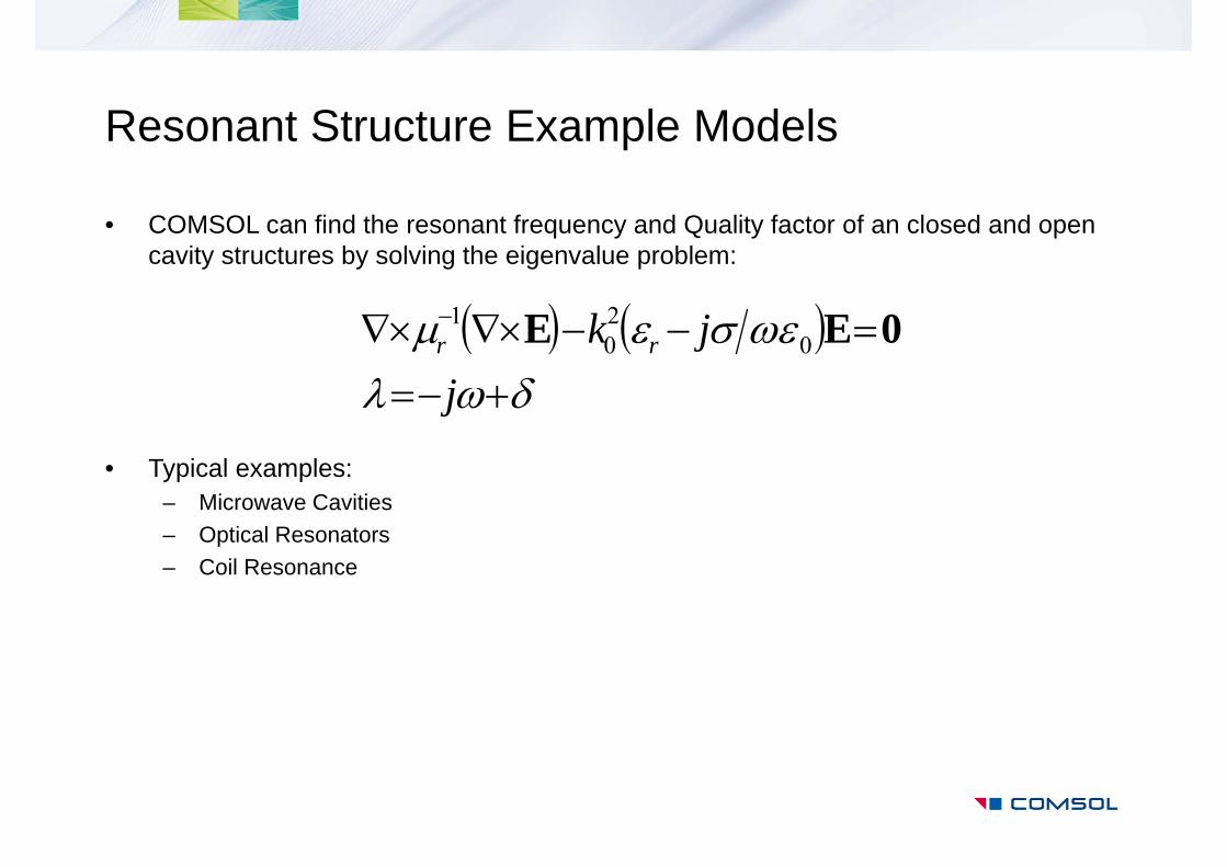
Resonant Structure Example Models
• COMSOL can find the resonant frequency and Quality factor of an closed and open cavity structures by solving the eigenvalue problem:
• Typical examples:– Microwave Cavities– Optical Resonators– Coil Resonance
jjk rr 0EE 0
20
1
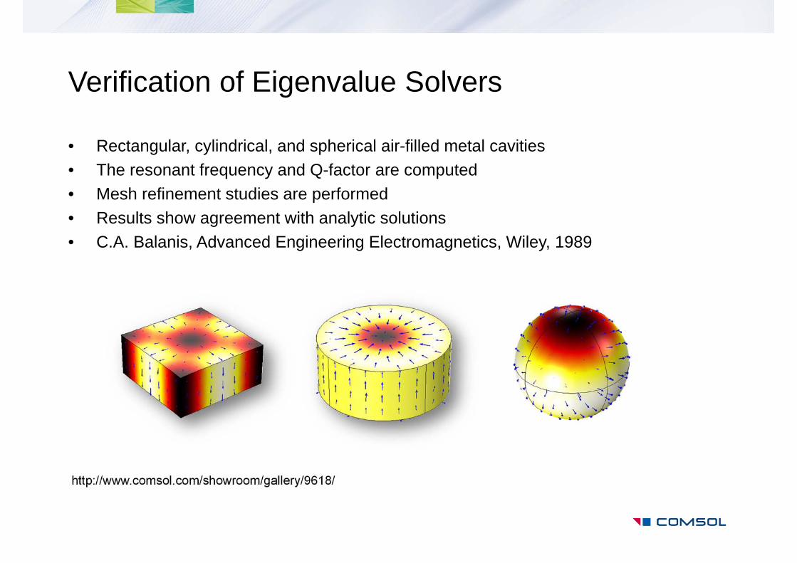
Verification of Eigenvalue Solvers
http://www.comsol.com/showroom/gallery/9618/
• Rectangular, cylindrical, and spherical air-filled metal cavities• The resonant frequency and Q-factor are computed• Mesh refinement studies are performed• Results show agreement with analytic solutions• C.A. Balanis, Advanced Engineering Electromagnetics, Wiley, 1989

Waveguides and Transmission Lines
• Any structure that guides electromagnetic waves along its structure can be considered a waveguide. COMSOL can compute propagation constants, impedance, S-parameters by solving:
• COMSOL also solves the time-harmonic transmission line equation for the electric potential for electromagnetic wave propagation along one-dimensional transmission lines :
• Typical examples:– Coaxial cable– Waveguides
z
rr
jyx
jk
z)exp( ,0
20
1
EE0EE
01
VCiG
xV
LiRx

Connecting a 3D RF Model to a Circuit Model
http://www.comsol.com/showroom/gallery/10833/
• A 3D model of a coaxial cable is connected to a circuit model• The source, and source impedance is modeled by the circuit model, as is the load
on the cable

Coaxial Cable to Waveguide Coupling
http://www.comsol.com/showroom/gallery/1863/
• A model of a coaxial cable feed that excites a propagating wave inside a rectangular waveguide
• S-parameters for transmission and reflection are computed
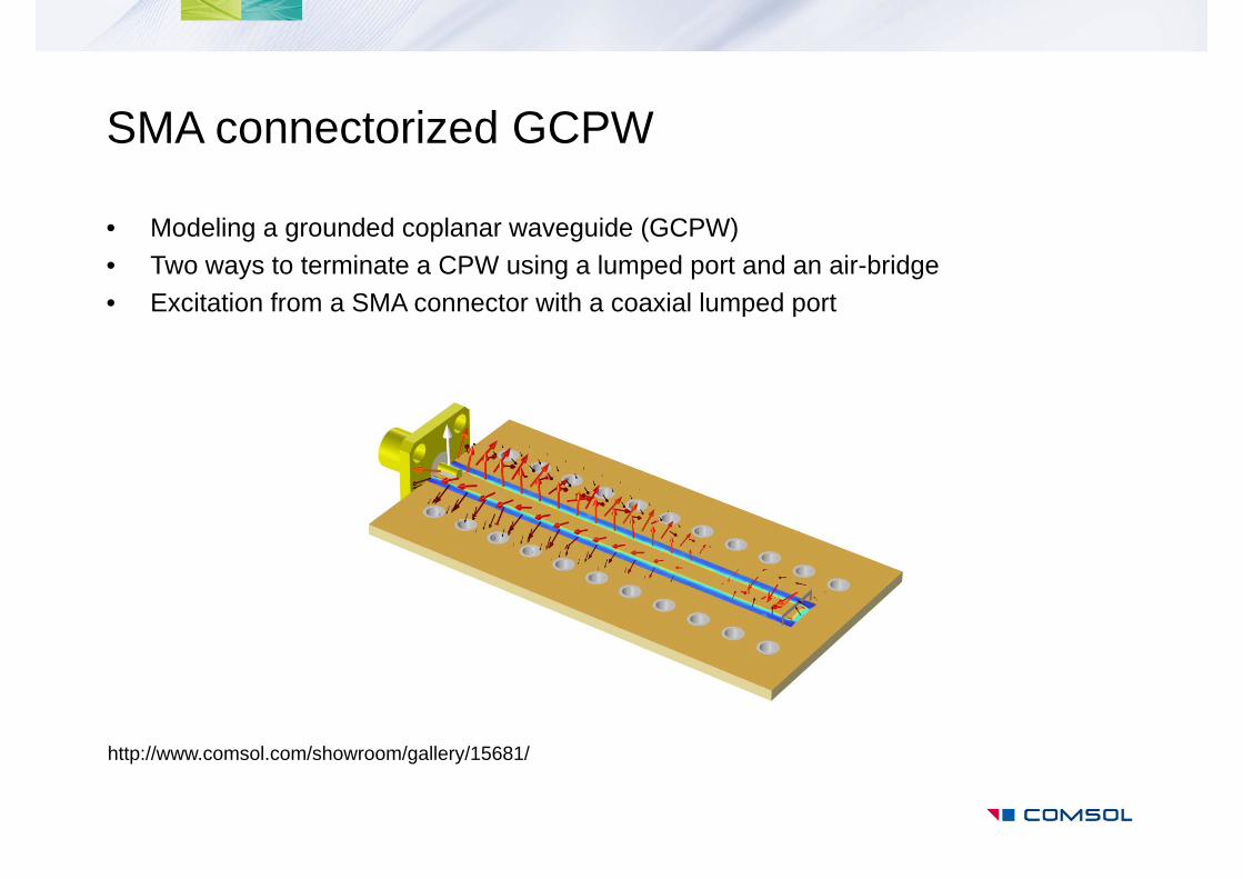
SMA connectorized GCPW
http://www.comsol.com/showroom/gallery/15681/
• Modeling a grounded coplanar waveguide (GCPW)• Two ways to terminate a CPW using a lumped port and an air-bridge• Excitation from a SMA connector with a coaxial lumped port

Dielectrophoresis (DEP) with an RF circuit
• Analyzing forces on dielectric particles under a non-uniform E-field• Electromagnetic Waves + Laminar Flow + Particle Tracing• E-field on CPW + Pressure and velocity in a microfluidic channel +
Newtonian particle motion due to drag, gravity and dielectrophoreticforces
Grounded coplanar waveguide (CPW) circuit excited at 100 MHz via an SMA connector and terminated with 50 ohm SMD resistor
Collecting particles due to dielectrophoretic forces

Passive Devices Example Models
• Passive devices like couplers, power dividers, and filters can be realized by combining resonant structures and transmission lines. COMSOL calculates the fields distribution, impedance, and S-parameters:
• Typical examples:– 3dB Couplers and Power Dividers– Band-pass Filters
nnn
n
rr
SS
SSSSS
S
jk
...:::::...
..
1
2221
11211
020
1 0EE

Frequency Selective Surface, CSRR
http://www.comsol.com/showroom/gallery/15711/
• One unit cell of the complementary split ring resonator (CSRR) with periodic boundary conditions to simulate an infinite 2D array
• Interior port boundaries combined with perfectly matched layer absorbing higher order modes

• Tunable the capacitance inside the cavity by the piezoelectric device • The resonant frequency is controlled by the capacitance • Higher voltage, thinner gap, more reactance, and lower frequency resonance
Tunable Evanescent Mode Cavity Filter Using a Piezoelectric Device
http://www.comsol.com/showroom/gallery/12619/

Antenna Example Models
• Antennas transmit and/or receive radiated electromagnetic energy. COMSOL can compute the radiated energy, far field patterns, losses, gain, directivity, impedance and S-parameters by solving the linear problem for the E-field:
• Typical examples:– Microstrip Patch Antenna– Vivaldi Antenna– Dipole Antenna
dSjkjkjk
far
rr
)exp(η4 000
020
1
rrHnrEnrE
0EE

Vivaldi Antenna
http://www.comsol.com/showroom/gallery/12093/
• A tapered slot antenna, also known as a Vivaldi antenna• Useful for wide band applications• An exponential function is used for the taper profile

Corrugated Circular Horn Antenna
http://www.comsol.com/showroom/gallery/15677/
• Designed using a 2D axisymmetric model• Low cross-polarization at the antenna aperture by combining TE mode excited at the
circular waveguide feed and TM mode generated from the corrugated inner surface

Examples of Scattering Problems
• An background electromagnetic field of known shape, such as a plane wave, interacts with various materials and structures. The objective is to find the total field and scattered fields by solving:
• Typical examples:– Mie Scattering– Radar Cross Section (RCS) calculations
scatteredbackgroundtotal
totalrtotalr jkEEE
0EE
0
20
1

Mie Scattering, Radar Cross Section of a Metal Sphere
http://www.comsol.com/showroom/gallery/10332/
• A sphere of metal is treated as a perfect electric conductor• Plane wave irradiates the sphere• Symmetry reduces the problem size• Second order elements represent the sphere shape to high accuracy• A Perfectly Matched Layer (PML) truncates the modeling domain• Far-field calculation computes the backscattered field• Results agree with analytic solution

User-defined Electric Displacement Example
• COMSOL can generate harmonics via a transient wave simulation, using nonlinear material properties:
rr
rrr tttDED
0DAAA
0
0001
Remanent electric displacement
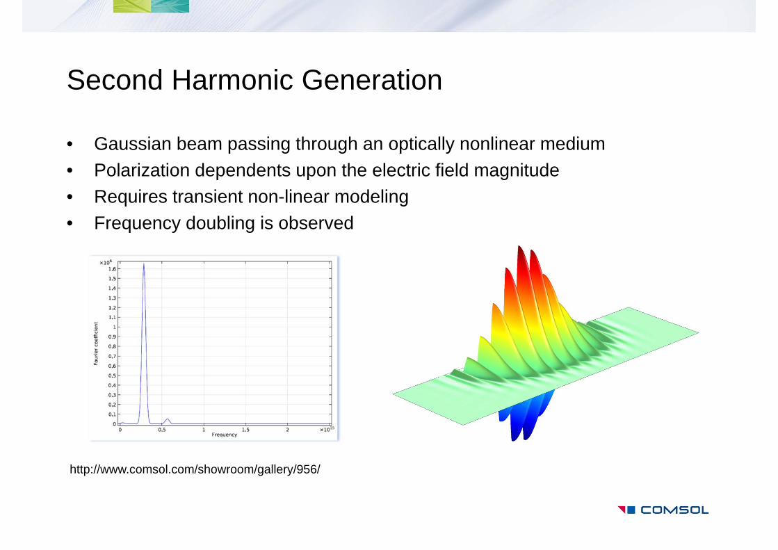
Second Harmonic Generation
http://www.comsol.com/showroom/gallery/956/
• Gaussian beam passing through an optically nonlinear medium• Polarization dependents upon the electric field magnitude• Requires transient non-linear modeling • Frequency doubling is observed

Examples of Periodic Problems
• Any structure that repeats in one, two, or all three dimensions can be treated as periodic, which allows for the analysis of a single unit cell, with Floquet Periodic boundary conditions:
• Typical examples:– Optical Gratings– Frequency Selective Surfaces– Electromagnetic Band Gap Structures
))(exp( sdFsd j rrkEE

• A 2D array of silver cylinders patterned on a substrate is modeled with one unit cell using Floquetperiodicity
• Higher-order diffraction is captured
Plasmonic Wire Grating
http://www.comsol.com/showroom/gallery/10032/
• The 2D model can be easily expanded to 3D using periodic port.

Electromagnetic Heating Examples
• An electromagnetic wave interacting with any materials will have some loss that leads to rise in temperature over time. Any losses computed from solving the electromagnetic problem can be bi-directionally coupled to the thermal equation:
• Typical examples: – Thermal Drift in a Microwave Filter Cavity– Microwave Ovens– Absorbed Radiation in Living Tissue– Tumor Ablation
Losses
neticElectromagQTktTCp
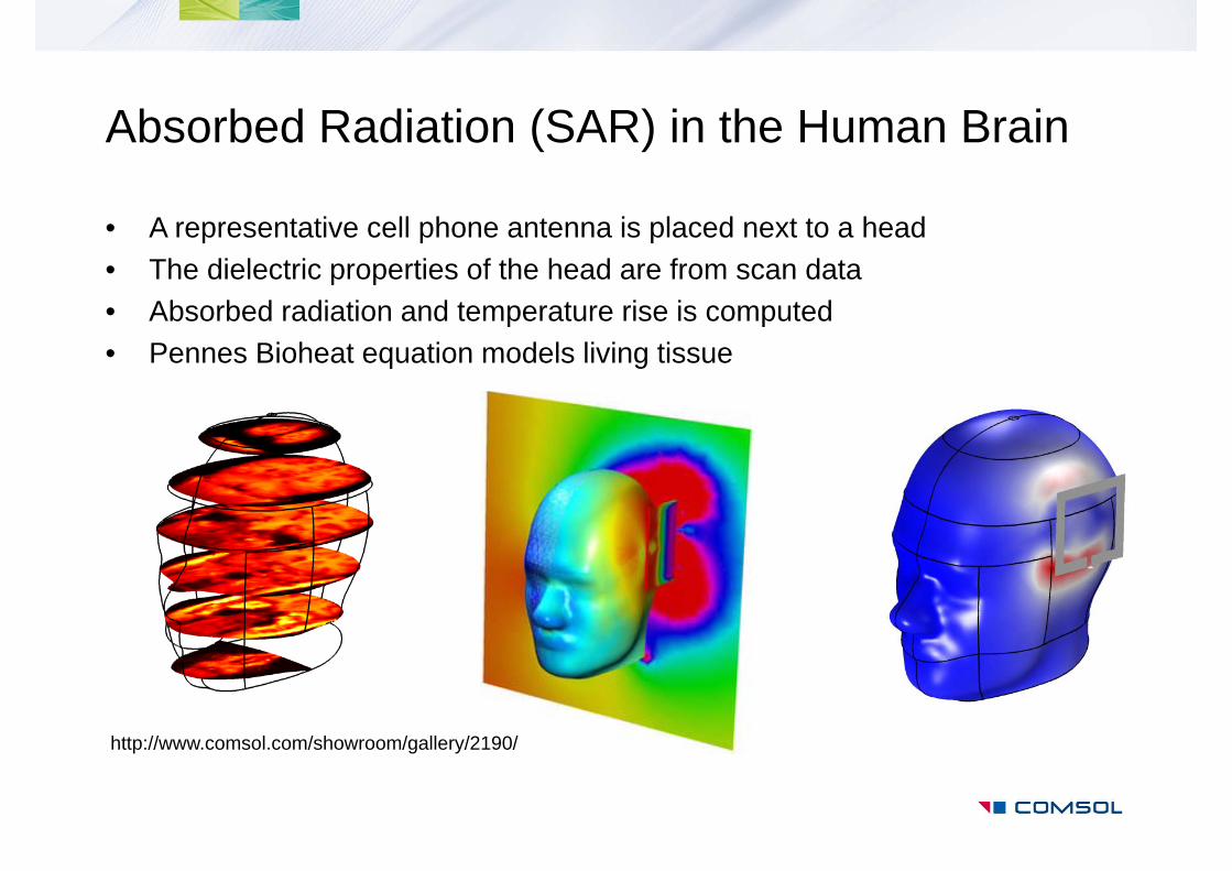
Absorbed Radiation (SAR) in the Human Brain
http://www.comsol.com/showroom/gallery/2190/
• A representative cell phone antenna is placed next to a head• The dielectric properties of the head are from scan data• Absorbed radiation and temperature rise is computed• Pennes Bioheat equation models living tissue