The retrospective iterated analysis scheme

RIC A RD o To D LIN G T Data Assimilation Ofice, N A SA/GSFC, Green belt, Mary land

July 11, 2002

Atmospheric data assimilation is the name scientists give to the techniques of blending atmospheric observations with atmospheric model results to obtain an accurate idea of what the atmosphere looks like at any given. time. Because two pieces of information are used, observations and model results, the outcomes of data assimilation procedure should be better than what one would get by using one of these two pieces of information alone. There is a number of different mathematical techniques that fall under the data assimilation jargon. In theory most these techniques accomplish about the same thing. In practice, however, slight differences in the approaches amount to faster algorithms in some cases, more economical algorithms in other cases, and even give better overall results in yet some other cases because of practical uncertainties not accounted for by theory. Therefore, the key is to find the most adequate data assimilation procedure for the problem in hand.

In our Data Assimilation group we have been doing extensive research to try and find just such data assimilation procedure. One promising possibility is what we call retro- spective iterated analysis (RIA) scheme. This procedure has recently been implemented and studied in the context of a very large data assimilation system built to help predict and study weather and climate. Although the results from that study suggest that the RIA scheme produces quite reasonable results, a complete evaluation of the scheme is very difficult due to the complexity of that problem. The present work steps back a little bit and studies the behavior of the RIA scheme in the context of a small problem. The problem is small enough to allow full assessment of the quality of the RIA scheme, but it still has some of the complexity found in nature, namely, its chaotic-type behavior. We find that the RIA performs very well for this small but still complex problem which is a result that seconds the results of our early studies.

'Additional affiliation: Science Applications International Corporation, Beltsville, Maryland.

1

https://ntrs.nasa.gov/search.jsp?R=20030034728 2018-06-26T15:47:11+00:00Z

,

The retrospective iterated analysis scheme for nonlinear chaotic dynamics*

RICARDO TODLING~ Data Assimilation Ofice, NASA/GSFC, Greenbelt, Maryland

To be submitted as a Note to the Monthly Weather Review

Abstract

Forecasts from lag-1 retrospective analyses are naturally better skilled than regular forecasts when verified one-lag ahead in time. This is not too surprising since these so called lag-1 retrospective forecasts have made use of the observations at the verification time. Because of their better quality one could conceive using these retrospective forecasts as background fields to recalculate previously calculated analyses. When this is done sequentially and intermittently it gives rise to a filtering procedure referred to as the retrospective iterated analysis (RIA) scheme. Implementation of this analysis strategy in the Goddard Earth Observing System (GEOS) Data Assimilation System (DAS) has recently been shown to improve the overall quality of the assimilation products. In the present short article we evaluate the performance of the RIA scheme for Lorenz (1963) dynamics. In this context, Monte Carlo simulations can be used to properly evaluate the performance of the scheme. The results show that for this type of dynamics the benefits from the RIA scheme are non-negligible in comparison to more standard procedures, such as the extended Kalman filter. These results are a second confirmation of the benefits from the RIA scheme observed in the GEOS DAS implementation.

1. INTRODUCTION

The fixed-lag Kalman smoother was introduced by Cohn et al. (1994) as a means to perform retro- spective data assimilation. This procedure presents a way of extracting information from the observations beyond what is usually extracted by filtering techniques such as three-dimensional variational analysis or four-dimensional schemes such as the extended Kalman filter (EKF). Smoothing in general operates not only by using observations in the past and present time of the estimate, as in filtering, but also by using observations a t future times. In particular, a fixed-lag smoother of lag e estimates the state at time tk by combining a filter estimate obtained using observations before and a t time tk with observations past time tk up to time tk+& for e 2 1. The fixed-lag Kalman smoother is an extension of the Kalman filter providing this type of enhanced correction to the filter estimates (e.g., see Chapter 7 of Anderson and Moore 1979, for more details). In the context of sequential estimation the fixed-lag smoother technique (an extension of the fixed-point smoother) is a natural extension of the underlying sequential filtering strategy.

In its original formulation, fixed-lag analyses are produced as a replacement of the usual filter analyses. Because fixed-lag analyses are expected to be of superior quality than the filter analyses it is conceivable to design iterative procedures in which the fixed-lag analyses feed back into the filter to try and enhance the quality of the overall filter. Todling (2000) proposed a feedback-type procedure in which, at a each analysis time, the analysis from a lag-1 smoother is used to recalculate the background field used in the filtering procedure. Therefore, a revised filter analysis can be produced using the retrospective (lag-1)

MD 20771, USA. e-mail: todling@dao.gsfc.nasa.gov. *Corresponding author address: Dr. Ricardo Todling, Data Assimilation Office, NASA/GSFC, Code 910.3, Greenbelt,

t Additional affiliation: Science Applications International Corporation, Beltsville, Maryland.

forecast as background instead of the original background. In linear optimal filtering and smoothing it can be shown that these retrospective forecasts are no more accurate than the original filter analyses and therefore an iterative procedure such as this does not result in any enhancement of the filtering results. However, in suboptimal situations, including the case of filters developed for nonlinear dynamics, this retrospective iterated analysis (RIA) scheme may prove useful. Indeed, Zhu et al. (2002) have recently implemented the RIA scheme in the Goddard Earth Observing System (GEOS) Data Assimilation System (DAS) and have found it to yield an overall improvement in the quality of the assimilated fields.

The purpose of this short communication is to show that the RIA scheme provides significant improve- ments also when applied to strongly nonlinear dynamics. In what follows we introduce in section 2 the RIA scheme in the context of the EKF, and show in section 3 how the results of the EKF compare with those of the RIA scheme when applied to the Lorenz (1963) dynamics. Conclusions appear in section 4.

2. BACKGROUND

Introductions to the EKF can be found elsewhere in the literature (e.g., Jazwinski 1970, Theorem 8.1). In the case of autonomous nonlinear dynamics and linear observation system these equations can be written as

WLlk-1 = M ( W i - I l k - 1 ) 7 (14

(1b)

( IC)

(14

(le)

f P k l k - 1 = M k ,k - 1 (wi- 1 lk - 1 )Pi - 1 lk - iM;f,k - 1 (wi- 1 - 1) + Qk 7

Wtlk = w,flk-l + Kklk (Yi - HkWLlk-l) ,

Kklk = PLlk-1HT(HkPil&-1HT + Rk)-l 9

p;lk = (I - KkJkHk)P:lk-l(I - Kk(kHkIT + KklkRkK;Slk ,

where the dynamical propagation expressions ( la) and (lb) obtain the n-dimensional forecast state and n x n-dimensional forecast error covariance, respectively, with the n x n matrix M k , k - l ( w ~ - l l k - l ) being the Jacobian of the nonlinear dynamical operator M,

This Jacobian is more commonly referred to as the tangent linear model, since it represents a series of consecutive linearizations around a reference trajectory initialized from wi- I , k - 1. The expressions (IC) and (Id) give the analysis state and analysis error covariance, respectively, when the pk-vector y i of observations become available at time t k . In the EKF the correction due to the observations is made through the Kalman gain matrix (le). The subscript notation follows that of Cohn et al. (1994), and briefly means that the n-vector wklj refers to an estimate valid at time t k obtained using observations up to and including observations at time t j .

In the corresponding nonlinear extension of the linear fixed-lag Kalman smoother of Cohn et al. (1994; e.g., see Todling and Cohn 1996) a correction to the analysis ~ z - ~ ~ ~ - ~ a t t k - 1 can be obtained for any lag L and is naturally denoted by ~ i - ~ ~ ~ + ~ . In the present article only the lag L = 1 case is of interest. The lag-1 correction to the filter analysis a t time t k - 1 , accounting for the observations a t time t k , can be obtained through the expressions

W i - l l k = W i - 1 J k - l + Kk-llk (Yi - HkW:lk-l) ,

P i - l l k = (I - Kk-llkHkMk,k-l(Wi-l~k-l)) T

(3a)

(3b) P i - l l k - 1 ,

where the second equation expresses the retrospective analysis error covariance matrix. Both wg- P,"-llk depend on the n x p k retrospective weight matrix Kk-llk,

and

K ~ - ~ ~ ~ = ~ i - l l k ~ l ~ ~ , k - l ( ~ ~ ~ l l k ~ l ) ~ ~ ( ~ k ~ ~ l k ~ l ~ ~ + ~ ~ 1 - l . (4)

In its original formulation the fixed-lag (retrospective) analyses ~ i - ~ ~ ~ are created at each time t k and left as a second sequence of estimates (the first being the sequence of filter analyses). If the smoothing procedure is working properly this second sequence of (retrospective) analyses should be of better quality than the sequence of filter analyses. In particular, we can forecast from the lag-1 analyses for a time interval corresponding to a single lag = 1, that is,

and build a sequence of retrospective forecasts + i l k . In the linear optimal case, it can be shown that this sequence of forecasts is better skilled than the sequence of forecasts w ~ l k - l . This is not surprising since these retrospective forecasts use the observations a t the times they are valid for. Indeed, it can also be shown that these retrospective forecasts are no more skillful than the filter analyses w i l k . This is also not surprising since in the linear optimal case, the Kalman filter provides the best linear unbiased estimate and therefore no other estimate can exceed its quality when the same observations are used.

However, in the nonlinear case these statements are not necessarily true. As a matter of fact, it is indeed possible that the retrospective forecasts may be of better quality than the original filter analyses. The experiments of Zhu et a1 (2002) with a lag-1 retrospective analysis system built for GEOS DAS show that this is indeed the case in that system. This motivates using the retrospective forecasts to recalculate the filter estimates as the filter goes along in time. For instance, in the EKF case, once the lag-1 retrospective analysis has been calculated a t time t k - 1 , say, we can calculate the retrospective forecast (5) and recalculate the filter analysis (IC) by replacing the background field wLlkWl with G - L l k .

This leads to an iterative procedure that can be repeated further for each time t k , that is, the newly recalculated analysis can be further corrected through another lag-1 smoother calculation, and so on. The resulting procedure is referred to as the retrospective iterated analysis (RIA) scheme. Notice that in the EKF context to recalculate the filter analysis properly the entire filter should be recalculated, that is, we should calculate (1) again starting from the retrospective analysis (3a) and retrospective forecast (5). Specifically, the second pass of the filter becomes

e i 1 k = Mk,k-l(WkO-lJk)Pi-lJkMT,k-l(WkO-llk) + Q k ,

% i l k = + i l k + K k l k ( y i - H k G i l k )

* i l k = ( I - k l k H k ) * { ( k ( I - K k ~ k H k ) ~ -t K k l k R k K r p , (6c)

K k l k = P i l k H ; f ( H k I ’ [ l k H T + R k ) - ’ .

( 6 4

(6b)

(6d)

Just as when the observation operator H k is nonlinear and an iterated extended Kalman filter (Jazwin- ski 1970, Theorem 8.2) can be developed, essentially based on Newton-type methods for solving nonlinear equations, here too, we can think of the re-feeding of the lag-1 retrospective analyses as a Newton-type iteration. Indeed one finds an iterated filter-smoother procedure in Jazwinski (1970; Theorem 8.3) that much resembles the RIA procedures above and is equally aimed at providing incremental corrections due to nonlinear dynamics, the difference being the RIA is based on a fixed-lag smoother where the iterated filter-smoother procedure is based on a fixed-interval smoother. Just as suggested in Todling (2000), and implemented in Zhu et al. (2002), here we are only interested in recalculating the filter analyses once per observation time, that is, we are interested in a single iteration only. In practice, analysis schemes are already computationally demanding and it may be difficult to justify more than a single iteration of the RIA scheme.

An obvious consequence of the RIA scheme is the introduction of correlation between errors of the (revised) background, that is, the retrospective forecasts, and the observations at each time. Indeed when showing that retrospective forecasts are no better than filter analyses in the linear optimal case these correlations need to be taken in to account. This means that, a t least in principle, equations (6) used to recalculate the filter analysis should be modified accordingly. Precisely, it is the weighting matrix K k l k

in (6d) and the corresponding analysis error covariance matrix @ilk in (6c) that should be modified. These modifications follow standard filter modifications when the the background and observations are

correlated (e.@;., Jazwinski 1970, Example 7.5). However, in general there is no guarantee that taking these correlations into account is beneficial in the nonlinear case. As a matter of fact, experiments performed for the dynamical system of the following section indicate deterioration of the results in some cases when accounting for this correlation (results not shown). Ignoring the correlation in the second pass filter (6) is similar to ignoring equivalent correlations existing in the iterated EKF procedure use to handle nonlinear observation operators.

3. RESULTS

In this section we use the Lorenz (1963) equations to investigate the behavior of the RIA scheme. We refer to reader to Miller et al. (1999) and Verlaan and Heemink (2001) and references therein for a variety of data assimilation studies conducted using this set of equations. The Lorenz (1963) equations

i = 4 Y - $1 1 ( 7 4

are applied here using the common set of parameters resulting in chaotic behavior: u = 10, p = 28, and ,B = 8/3. As in Miller et al. (1994) the true state evolution is simulated from a deterministic integration of these equations starting from the initial condition (2, y, z) (O) = (1.508870, -1.531271,25.46091). A fourth-order Runge-Kutta scheme is used to integrate (7) and to generate the true state trajectory. To make the problem somewhat more challenging we follow Evensen and Fario (1997) in choosing a different finite-difference scheme to integrate the equations when using them as the forecast model M in (la) and (5). For this purpose we use a second-order predictor-corrector scheme. Its corresponding Jacobian necessary for the EKF and RIA schemes is calculated following Miller et al. (1994). With different discretizations for the evolution of the truth and the prediction model the experiments conducted here are not quite of the identical twin-type. All experiments are taken up to 20 (dimensionless) time units. Both finite difference schemes use At = 0.00625 and observations are taken a t time intervals Atobs = 40At, that is, the true state is sampled every 0.25 time units. The observation errors are uncorrelated and drawn from a mean-zero Gaussian distribution with variance 4. [Fig. 1 near here, please.]

Miller et al. (1994) have shown that the EKF can be turned into a useful assimilation scheme for highly nonlinear dynamical systems such as (7) if, for example, a reasonable specification of model error is provided. Since, in this idealized exercise, we have access to the true state, we estimate the model error covariance matrix Q k needed in ( lb) through a Monte Carlo simulation using 10,000 Gaussian-distributed initial conditions with mean zero and variance 2 in each variable. Each initial condition is integrated from t = 0 to t = Atobs and a t the end of the 10,000 integrations the error covariance with respect to the true state is calculated a t t = Atobs. The resulting model error covariance

0.1628 0.2649 -0.0443 0.2649 0.4322 -0.0678

-0.0443 -0.0678 0.0566

is applied at each time step during the EKF forecast error covariance evolution calculation. This model error covariance expresses both the effect of the distinct initial conditions used in the Monte Carlo simulation as well as the distinction in the finite-difference schemes used to generate the true and forecast states. This specification of the model error covariance is distinct from that of Miller et al. (1994) which is an attempt to capture the error due to linearization (2) necessary in the EKF. Though a more accurate description of model error can be devised in our case, the prescription here is simple and good enough to turn the EKF in our experiments into a reliable assimilation scheme for the dynamics in hand. [Fig. 2 near here, please.]

We evaluate the performance of all assimilation experiments through Monte Carlo simulations taking 10,000 samples from a similar distribution as that used to obtain the specification of the model error

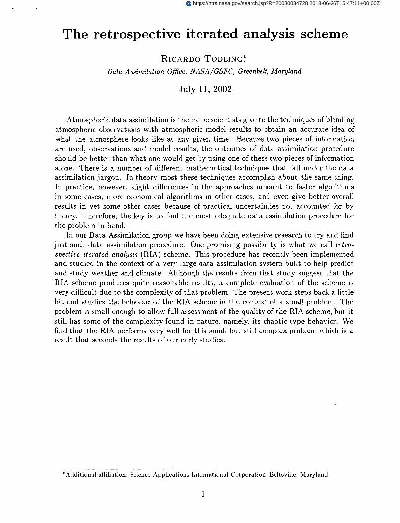
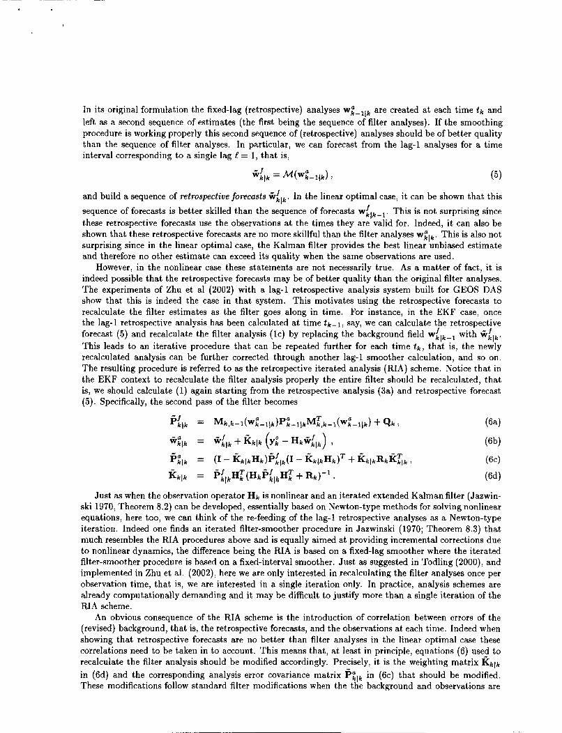
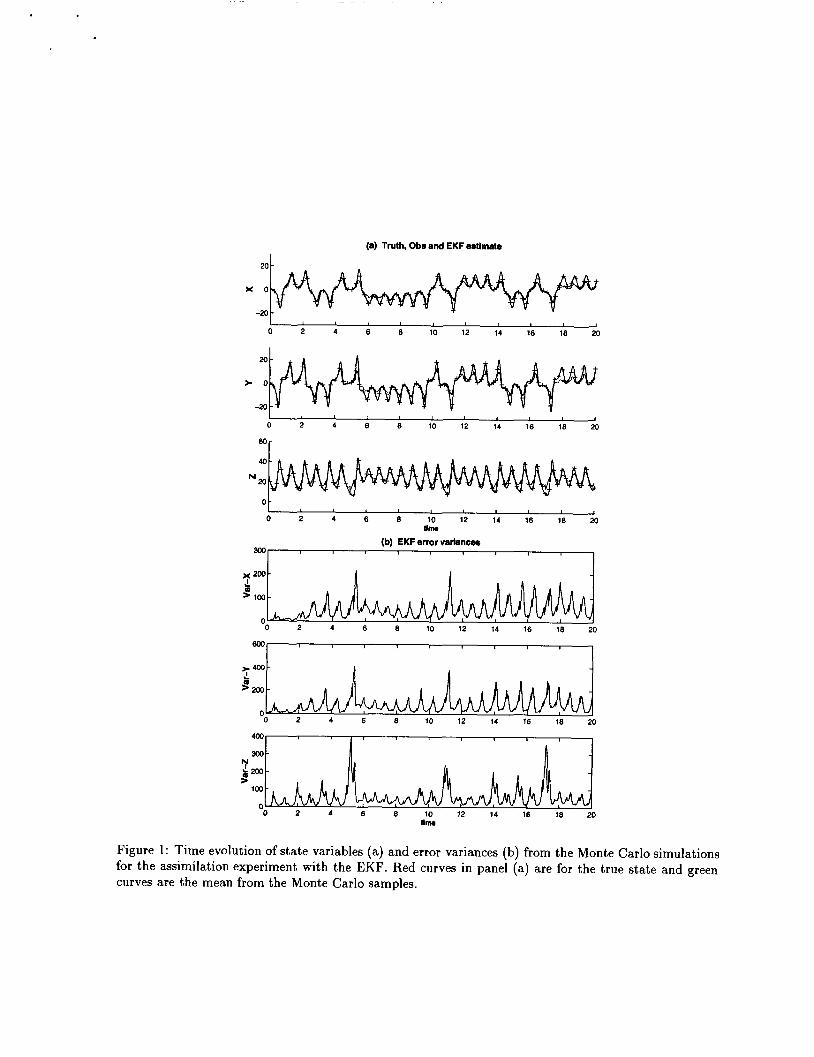
covariance matrix. This means in this case that we run 10,000 EKF experiments started from the 10,000 initial conditions and each experiment takes a different sequence of observational errors drawn from a normal distribution with mean zero and error variance 4 in each observed variable (e.g., see Maybeck 1982, section 9.5). Results from the Monte Carlo experiments for the EKF with the model error covariance matrix Q in (8) and when all three variables are observed are displayed in Fig. 1. The three plots in panel (a) show the true state evolution (red curves) and the mean state evolution from the Monte Carlo simulations (green curves); the three plots in panel (b) show the error variances calculated from the Monte Carlo samples for each variable. We see that the prescribed model error covariance Q in (8) is enough to keep the EKF from diverging most of the time. However, the EKF does not remain completely on track. This can certainly be blamed on the specification of model error covariance matrix used here. However, the point here is not to correct the EKF deficiencies directly but rather to show that the RIA scheme can be used to do so indirectly. The peaks of the error variances (panel b) indicate when the estimates from the EKF lose accuracy. These times are usually associated with regime transition times as Miller et al. (1994) have shown (compare peaks of large error variance about, say, t M 5.5, or t M 11, for example, with the state evolution around these times seen in panel a). [Fig. 3 near here, please.]

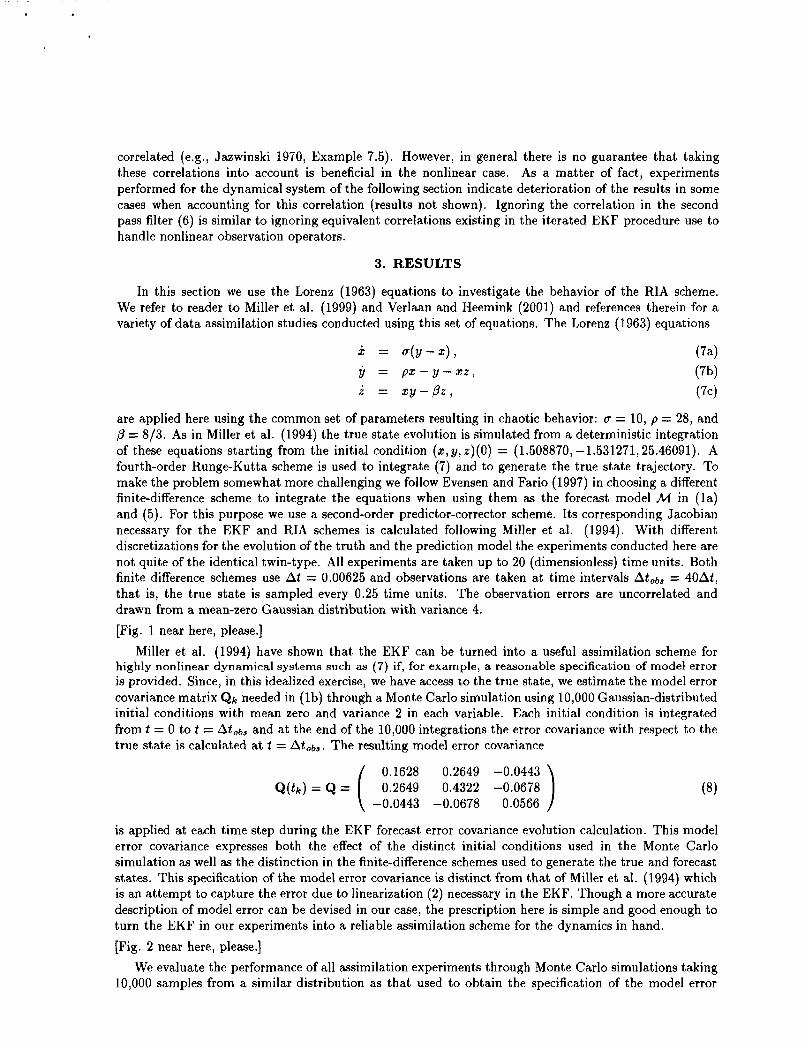
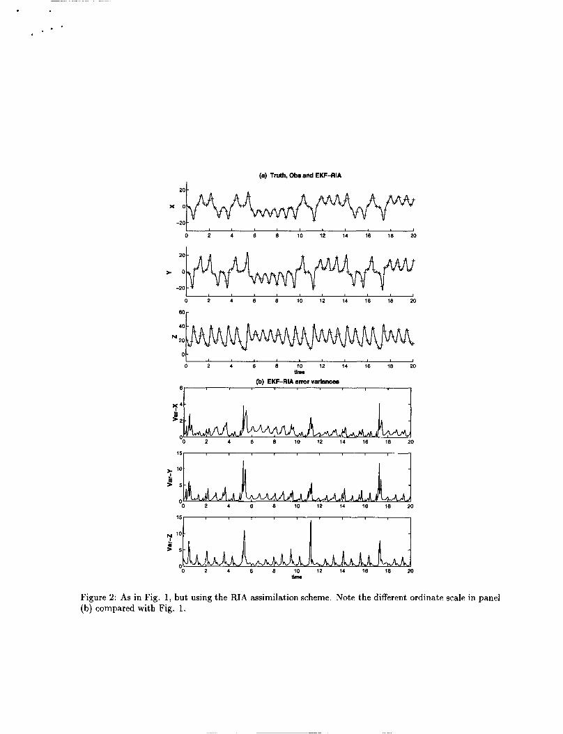
Again, a Monte Carlo simulation similar to that performed to evaluate the EKF was carried out to evaluate the RIA scheme. Results are displayed in Fig. 2. We see now directly from the mean state evolution of the RIA estimates (green curves in panel a) a much closer agreement with the truth than seen for the mean state evolution estimate from the EKF of Fig. 1. The error variance plots for the RIA (panel b of Fig. 2) show a dramatic error reduction when compared with the corresponding EKF plots of Fig. 1. The peaks of large errors are again near times of regime transitions due to the chaotic nature of the dynamics, but their magnitudes are now much smaller than the magnitude of the errors obtained when the EKF is used alone [notice scale difference in panels (b) of Figs. 1 and 21.

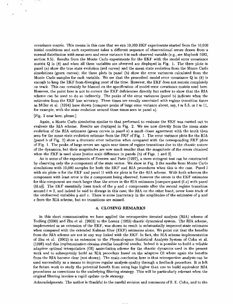
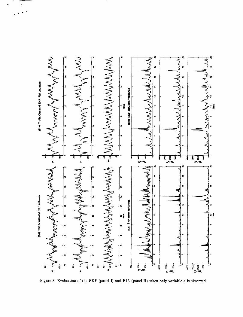
As in some of the experiments of Evensen and Fario (1997), a more stringent test can be constructed by observing only the z-component of the state vector. We show in Fig. 3 the results from Monte Carlo simulations with 10,000 samples for both the EKF and RIA procedures when this is the case. Panel I with six plots is for the EKF and panel I1 with six plots is for the RIA scheme. With both schemes the component with least error is the z component being observed, however the errors in the EKF estimates for this component are much larger than the errors in the RIA estimates [compare panel (La) with panel (II.a)]. The EKF essentially loses track of the y and E components after the second regime transition around t = 2, and indeed be said to diverge in this case; the RIA on the other hand, never loses track of the unobserved variables y and E . There is some inaccuracy in the amplitudes of the estimates of y and z from the RIA scheme, but no transitions are missed.

4. CLOSING REMARKS

In this short communication we have applied the retrospective iterated analysis (RIA) scheme of Todling (2000) and Zhu et a]. (2002) to the Lorenz (1963) chaotic dynamical system. The RIA scheme, implemented as an extension of the EKF, was shown to result in substantially improved state estimates when compared with the extended Kalman filter (EKF) estimates alone. We point out that the benefits from the RIA scheme are not in any way linked with the EKF. In fact, the RIA scheme implementation of Zhu et al. (2002) is an extension to the Physical-space Statistical Analysis System of Cohn et al. (1998) and this implementation obtains similar beneficial results. Indeed it is possible to build a reliable adaptive optimal interpolation (01) assimilation scheme for the chaotic dynamics used in the present work and to subsequently build an RIA procedure based on the adaptive 0 1 where again the benefits from the RIA become clear (not shown). The main conclusion here is that retrospective analysis can be used successfully as a means to improve regular analysis quality through a feedback procedure. It is left for future work to study the potential benefit from using lags higher than one to build equivalent RIA procedures as corrections to the underlying filtering strategy. This will be particularly relevant when the original filtering invokes a rapid update cycle strategy. Acknowledgments. The author is thankful to the careful revision and comments of S. E. Cohn, and to the

comments of Y. Zhu. This research was partially supported by the NASA EOS Interdisciplinary Project on Data Assimilation.

References Anderson, B. D. O., and J. B. Moore, 1979: Optimal Faltering. Prentice-Hall, 357 pp. Cohn, S. E., N. S. Sivakumaran, and R. Todling, 1994: A fixed-lag Kalman smoother for retrospective

data assimilation. Mon. Wea. Rev., 122, 2838-2867. Cohn, S. E., A. da Silva, J . Guo, M. Sienkiewicz, and D. Lamich, 1998: Assessing the effects of data

selection with the DAO physical-space statistical analysis system. Mon. Wea. Rev. , 126, 2913-2926. Evensen, G., and N. Fario, 1997: Solving for the generalized inverse of the Lorenz model. J. Meteorol.

Soc. Japan, 75 , 229-243. Jazwinski, A.H., 1970: Stochastic Processes and Filtering Theory. Academic Press, 376 pp. Lorenz, E. , 1963: Deterministic non-periodic flow. J . Atmos. Sci., 20, 130-141. Maybeck, P. S . , 1982: Stochastic models, estimation, and control. Vol. 2, Academic Press, 291 pp. Miller, R. N., M. Ghil, and F. Gauthiez, 1994: Advanced data assimilation in strongly nonlinear dynamical

systems. J. Atmos. Sci., 58, 1037-1056. Miller, R. N., E. F. Carter Jr., and S. T . Blue, 1999: Data assimilation into nonlinear stochastic models.

Tellus, 51A, 167-194. Todling, R., 2000: Retrospective data assimilation schemes: fixed-lag smoothing. Proc. Second Zntl.

Symp. Frontiers of Time Series Modeling: Nonpammetric approach to knowledge discovery, Nara, Japan , December , 155- 173.

Todling, R. and S. E. Cohn, 1996: Some strategies for Kalman filtering and smoothing. Proc. ECMWF Seminar on Data Assimilation, 91-111.

Verlaan, M., and A. Heemink, 2001: Nonlinearity in data assimilation applications: a practical method for analysis. Mon. Wea. Rev., 129, 1578-1589.

Zhu, Y., R. Todling, J . Guo, S. E. Cohn, I. M. Navon, and Y. Yang., 2002: The GEOS retrospective data assimilation system: the 6-hour lag case. Mon. Wea. Rev., submitted.

Figure Captions Fig. 1: Time evolution of state variables (a) and error variances (b) from the Monte Carlo simulations

for the assimilation experiment with the EKF. Red curves in panel (a) are for the true state and green curves are the mean from the Monte Carlo samples.

Fig. 2: As in Fig. 1, but using the RIA assimilation scheme. Note the different ordinate scale in panel (b) compared with Fig. 1.

Fig. 3: Evaluation of the EKF (panel I) and RIA (panel 11) when only variable X is observed.

(a) Truth, Obs and EKF estlrnata

20

x o

-20 I I

0 2 4 6 8 10 12 14 16 18 20

20

* o

-20 I

0 2 4 6 8 10 12 14 16 18 20

40

N20

0 I

0 2 4 6 8 10 12 14 16 18 20 UnW

(b) EKF emf varbncmJ 1

X 2oJ L 3 loo

0 0 2 4 6 8 10 12 14 16 18 20

I L.

p m

' 0 2 4 8 8 10 12 14 16 18 20

300- N

0 2 4 6 8 10 12 14 16 18 20

Figure 1: Time evolution of state variables (a) and error variances (b) from the Monte Carlo simulations for the assimilation experiment with the EKF. Red curves in panel (a) are for the true state and green curves are the mean from the Monte Carlo samples.

((I) Truth, Ob8 end EW-RIA

20

x o

-20 I I I 0 2 4 6 8 10 12 14 16 16 20

20

-20

0 2 4 6 8 10 12 14 16 18 20

40

20

0 I

0 2 4 6 8 10 12 14 16 16 20 Urn.

@) EKF-RIA emr varlnncea 6

x 4 I ..

0 2 4 6 8 10 12 14 16 16 20

> lo L 2 5

0 0 2 4 6 8 10 12 14 16 16

"0 2 4 8 8 10 12 14 16 18 20 UIlU

Figure 2: As in Fig. 1, but using the RIA assimilation scheme. Note the different ordinate scale in panel (b) compared with Fig. 1.

d : Y 8 E 6 i s c' 4 1

c

8 0 8 X

R

e

F

f

-4 r

?

D

0

c

v

>

R

e

c

f

P

P

m

10

*

N

0

R

e

P

f

N

P

m

W

U

N

0

R

PD

F

f

b

P

D

c)

*

v

a

8 8 8 0 Z

% 8 R 0 Z

I 5

R

I

'0

f

N,

P

m

10

U

N

R

e

0

f

N

P

m

D

c

-4

a

8

I

P

f

N

P

m

10

U

N

Figure 3: Evaluation of the EKF (panel I) and RIA (panel 11) when only variable z is observed.