Embed Size (px)
Citation preview

JOURNAL OF FINANCIAL AND QUANTITATIVE ANALYSIS Vol. 45, No. 3, June 2010, pp. 555–587COPYRIGHT 2010, MICHAEL G. FOSTER SCHOOL OF BUSINESS, UNIVERSITY OF WASHINGTON, SEATTLE, WA 98195doi:10.1017/S0022109010000256
The Response of Corporate Financing andInvestment to Changes in the Supply of Credit
Michael Lemmon and Michael R. Roberts∗
Abstract
We examine how shocks to the supply of credit impact corporate financing and investmentusing the collapse of Drexel Burnham Lambert, Inc.; the passage of the Financial Insti-tutions Reform, Recovery, and Enforcement Act of 1989; and regulatory changes in theinsurance industry as an exogenous contraction in the supply of below-investment-gradecredit after 1989. A difference-in-differences empirical strategy reveals that substitution tobank debt and alternative sources of capital (e.g., equity, cash balances, and trade credit)was limited, leading to an almost one-for-one decline in net investment with the declinein net debt issuances. Despite this sharp change in behavior, corporate leverage ratios re-mained relatively stable, a result of the contemporaneous decline in debt issuances and in-vestment. Overall, our findings highlight how even large firms with access to public creditmarkets are susceptible to fluctuations in the supply of capital.
I. Introduction
Fluctuations in the supply of financial capital flowing to different sectors ofthe market can be extreme.1 Coupled with the presence of financing frictions,
∗Lemmon, [email protected], Eccles School of Business, University of Utah, 1645 E.Campus Center Dr., Rm. 109, Salt Lake City, UT 84112; Roberts, [email protected],Wharton School, University of Pennsylvania, 3620 Locust Walk, Ste. 2300, Philadelphia, PA 19104.We are especially grateful for helpful comments from an anonymous referee, Paul Malatesta (the ed-itor), and Mitchell Petersen. We also thank Andy Abel, Marshall Blume, David Chapman, DarrellDuffie, Itay Goldstein, Joao Gomes, Wei Jiang, Arvind Krishnamurthy, Augustin Landier, DavidMatsa, Andrew Metrick, Toby Moskowitz, Stewart Myers, Vinay Nair, Josh Rauh, Andreea Roman,Nick Souleles, Phil Strahan, Amir Sufi, Petra Todd, Greg Udell, Toni Whited, Julie Xu, andRebecca Zarutskie; seminar participants at Boston College, Massachusetts Institute of Technology,Northwestern University, Norwegian School of Management (BI), Stanford University, University ofArizona, University of Chicago, University of Indiana, University of Pennsylvania, and University ofWisconsin-Madison; and conference participants at the 2006 University of British Columbia SummerFinance Conference and 2007 Princeton/New York Federal Reserve Conference on Liquidity. Robertsgratefully acknowledges financial support from a Rodney L. White Grant and an NYSE ResearchFellowship.
1As recently noted in BusinessWeek (January 29, 2007): “Foreign investors are shipping gobsof cash into the U.S. At the same time, there has been an explosion of hedge funds, distressed debttraders, and others eager to buy junk-rated debt for the higher yields it offers. . . . Together, these factorshave combined to create unheard-of pools of liquidity [that have] made funding readily available [to]companies.”
555

556 Journal of Financial and Quantitative Analysis
such as adverse selection (e.g., Stiglitz and Weiss (1981)) or moral hazard (e.g.,Holmstrom and Tirole (1997)), these fluctuations can impact financing and in-vestment. In this paper we study how changes in the supply of capital affect firmfinancing and investment by focusing on the sharp decline of capital flows to thespeculative-grade debt market that occurred in 1989.
Understanding whether the supply of capital corresponds to a separate chan-nel, independent of demand, through which market imperfections influence cor-porate behavior, is important for several reasons. First, the supply of capital mayplay an important role in the transmission of monetary policy (Bernanke andGertler (1989), Kashyap, Lamont, and Stein (1994)). Second, fluctuations in thesupply of capital may play an important role, more generally, in determiningthe financial and investment policies of firms, outside of monetary policy regimechanges (Faulkender and Petersen (2006), Leary (2007), and Sufi (2009)). Finally,surveys of corporate managers and financial intermediaries suggest a dichotomyin how academics and practitioners tend to view financing decisions: The formerperceive decisions as governed by the demands of the users of capital; the lat-ter perceive decisions as governed by the preferences of the suppliers of capital(Titman (2001), Graham and Harvey (2001)).
However, identifying a linkage between the supply of capital and corporatebehavior is difficult because of the fundamental simultaneity occurring betweensupply and demand. This task is further complicated by an inability to preciselymeasure investment opportunities or productivity shocks. The goal of this paperis to address these issues and to identify the extent to which variations in the sup-ply of capital influence corporate financial and investment policies. To do so, weuse three near-concurrent events as an exogenous shock to the supply of creditto below-investment-grade firms after 1989: i) the collapse of Drexel BurnhamLambert, Inc. (Drexel); ii) the passage of the Financial Institutions Reform, Re-covery, and Enforcement Act of 1989 (FIRREA); and iii) a change in the NationalAssociation of Insurance Companies (NAIC) credit rating guidelines.
The disappearance of Drexel led to a significant reduction in capital availableto non-investment-grade firms by investors whose participation relied on Drexel’spresence as both an originator and intermediary (Benveniste, Singh, and Wilhelm(1993)). Likewise, the passage of FIRREA led to an immediate cessation of the$12 billion annual flow of capital to speculative-grade firms from savings andloans (S&Ls), while simultaneously forcing a sell-off of all junk bond holdingsby S&Ls. Finally, commitments by life insurance companies to purchase below-investment-grade debt fell by 60% in 1990 and continued to fall over the next 2years, after the NAIC changed its ratings of corporate debt to mimic those used bynationally recognized statistical rating organizations (NRSROs) (e.g., Moody’s,Standard & Poor’s (S&P)). Importantly, we show that the primary impetus foreach of the three events is largely removed from nonfinancial firms’ demandsfor financing and investment; that is, the shocks are exogenous with respect tofirm demand. In concert, these three events led to the near disappearance of themarket for below-investment-grade debt—both public and private placements—after 1989.
The specificity of these events to the speculative-grade debt market enablesus to employ a difference-in-differences empirical approach that helps to identify
Lemmon and Roberts 557
both the direction and magnitude of the supply shock’s impact on firm behavior.Our findings reveal that the supply shock had significant implications for the fi-nancing and investment behavior of below-investment-grade firms after 1989. Asa whole, below-investment-grade firms decreased their total net security issuances(debt plus equity) by approximately 5% of assets relative to a propensity-score-matched control group of unrated firms. Economically, this decline correspondsto a near halving of net security issuances relative to pre-1990 levels and is drivenentirely by a decline in net debt issuing activity, which fell by approximately 66%relative to pre-1990 levels. Additionally, we observe almost no substitution bybelow-investment-grade firms to alternative sources of financing such as equity,trade credit, or internal funds, and no change in dividend policy. The ultimateconsequence of this reduction in debt issuing activity and lack of substitution is aone-for-one decline in net investment of 5% of assets, a 33% decline relative topre-1990 levels.
We also investigate cross-sectional variation in the impact of the supplyshock by identifying variation in the costs of switching to alternative sourcesof funds. For example, bank lending contracted relatively more sharply in theNortheast part of the U.S. during 1990 and 1991—a consequence of eroding bankcapital driven by declining real estate prices (Bernanke and Lown (1991), Peekand Rosengren (1995)). This geographic heterogeneity in the availability of bankcredit and the fact that firms tend to borrow from local banks (Bharath, Dahiya,Saunders, and Srinivasan (2007)) enables us to use the location of firms’ head-quarters as an instrument to identify the impact of the contraction in intermediarycapital on firm behavior.
We show that below-investment-grade firms with headquarters located in theNortheast experienced a decline in net security issuing activity equal to 6% ofassets relative to the change experienced by below-investment-grade firms withheadquarters in other parts of the country. Again, this decline is concentrated al-most entirely in net debt issuing activity, with little or no substitution to alternativesources of finance. Consequently, net investment declined one-for-one (6%) withdecreased financing activity. Importantly, we show that these effects are foundonly among below-investment-grade firms; neither investment-grade nor unratedfirms reveal any significant changes in financing or investment behavior as a func-tion of geography, thereby ensuring that our findings are not a consequence ofgeographic heterogeneity in aggregate productivity shocks or the severity of the1990–1991 recession. Thus, for firms facing higher borrowing costs because ofless intermediary capital, we see a more pronounced response to the credit con-traction in the speculative debt market.
In addition to geographic heterogeneity, we also find that riskier below-investment-grade firms (those rated B+ or lower) had a different response to thecredit contraction relative to less risky below-investment-grade firms (those ratedBB– to BB+). Specifically, riskier firms experienced a sharper decline in net secu-rity issuances and net investment relative to their less risky counterparts. Riskierfirms also experienced a more protracted decline in net security issuances and netinvestment, lasting for 4 years after the shock. The more highly rated firms, on theother hand, experienced a meaningful change in financing and investment behav-ior for only the first 2 years following the shock. Thus, for riskier firms requiring

558 Journal of Financial and Quantitative Analysis
more monitoring or facing greater incentive problems, we also see a more pro-nounced response to the credit contraction.
Overall, our findings support the view that shifts in the supply of capitalcan have significant consequences for the financial and investment policies offirms, while our study makes three contributions. First, our examination of thespeculative-grade market is particularly revealing in that even firms with accessto public debt markets can be significantly affected by fluctuations in the supplyof credit.2 This result is somewhat surprising for several reasons. First, previousstudies that investigate how the supply of credit affects firm behavior have oftenused firms with access to public debt markets as a comparison or control group,implicitly assuming that these firms are relatively immune to credit supply fluctu-ations (e.g., Kashyap et al. (1994), Faulkender and Petersen (2006)).
A second reason is that speculative-grade firms are 4 times larger and 4 timesmore profitable than unrated, bank-dependent firms, on average. This character-istic also contrasts with results from previous work relying on large firms as acomparison group that is relatively immune to credit supply fluctuations (e.g.,Gertler and Gilchrist (1994), Leary (2007)). Finally, despite using relatively moredebt, speculative-grade firms are significantly financially healthier than unratedfirms, as indicated by higher Altman Z-scores. That is, counter to their colloquialname, “junk firms” are anything but marginal, excessively risky firms, on aver-age, when compared to the bank-dependent firms studied throughout much of theprevious literature. Thus, our results complement previous studies by showingthat the real effects of shocks to the supply of capital are not limited to small,bank-dependent firms.
Finally, our study also reveals that shocks to capital market sectors otherthan the banking sector can impact corporate behavior. Most previous studies fo-cus exclusively on shocks to bank capital or on the role of bank lending in influ-encing corporate behavior. For example, Gertler and Gilchrist (1994), Kashyap,Stein, and Wilcox (1993), and Kashyap et al. (1994) examine the impact of tightermonetary policy on corporate behavior. Sufi (2009) examines the introduction ofsyndicated loan ratings in 1995, while Leary (2007) examines the introduction ofthe certificate of deposit and binding interest rate ceilings that occurred during the1960s.3
The second contribution is that some of our results provide a contrast withrecent evidence suggesting an important role for the supply of credit in determin-ing leverage ratios. Interestingly, though net debt issuing activity contracted quitesharply in our sample, we find that the combined effect of reduced debt issuancesand investment results in relatively stable leverage ratios for below-investment-grade firms during this period. This finding differs from those of Faulkender and
2New junk bond issuances have averaged $127 billion per year since 2002, when new issuanceswere $62 billion, according to Moody’s. Leveraged loan (i.e., high-yield credit agreements) issuanceshave tripled since 2002, increasing to $480 billion last year, according to S&P’s Leveraged Commen-tary and Data (LCD) unit.
3Other studies examining the effect of shocks to the banking sector on firm behavior include Chavaand Purnanandam (2006), who examine the short-run impact of the Russian crisis on bank-dependentborrowers’ equity returns, and Zarutskie (2006), who examines the impact of the Riegle-Neal Act onnewly formed firms.

Lemmon and Roberts 559
Petersen (2006), Sufi (2009), and Leary (2007), all of whom suggest that supplyshifts significantly impact corporate leverage. Thus, the role played by supply-side factors in determining variation in leverage ratios is, perhaps, limited to par-ticular instances.
While our study falls short of a controlled experiment, we believe that ittakes an important step forward relative to previous studies in terms of addressingthe basic identification problem of disentangling supply-side and demand-sideforces. Indeed, Oliner and Rudebusch ((1996), p. 308) emphasize this identifi-cation problem by arguing that it is the “shortcoming of most previous empir-ical work on the bank lending channel.” Our study investigates a local supplyshock affecting a well-defined segment of the corporate population, which pro-vides for a more natural treatment-control delineation relative to previous stud-ies that investigate broader shocks affecting all firms (or all public firms). Wealso explicitly examine the identifying assumption (i.e., the “parallel trends” as-sumption) behind the difference-in-differences framework. Finally, by investigat-ing cross-sectional variation in the corporate response to the supply shock, weare able to point to a specific source of exogenous variation (i.e., the geographiclocation of firms’ headquarters) that we use to identify the impact of the creditcontraction.
The remainder of the paper proceeds as follows. Section II describes theevents generating the supply shock and the economic environment surroundingthe shock. Section III discusses various theories of why fluctuations in the supplyof capital might affect corporate behavior. Section IV introduces the data and thebasic empirical strategy. Section V presents the results of our analysis. Section VIconcludes.
II. Background and Macroeconomic Environment
The goal of this section is threefold. First, we establish a link between thethree events and the supply of capital to below-investment-grade firms. Second,we argue that these three events are largely exogenous with respect to nonfi-nancial corporate demand for debt financing and investment. Finally, we discussthe macroeconomic environment surrounding our time period of interest, payingclose attention to the recession occurring in 1990 and 1991. References to theliterature surrounding these issues are provided for further details.
A. The Rise and Fall of Speculative-Grade Credit
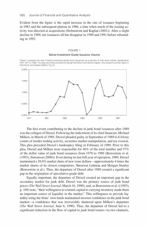
Prior to 1977, junk bonds consisted primarily of bonds originally issuedas investment-grade securities that were subsequently downgraded to specula-tive grade, so-called “fallen angels” (Simonson (2000)). Shortly after 1977, firmsbegan issuing a nonnegligible amount of speculative-grade securities (Asquith,Mullins, and Wolff (1989)). Figure 1 presents the rate of issuance for speculative-grade bonds, expressed as a percentage of total stock market capitalization.4
4We are grateful to Bengt Holmstrom and Steve Kaplan for allowing us to reproduce this figurefrom Holmstrom and Kaplan ((2001), Fig. 5).
560 Journal of Financial and Quantitative Analysis
Evident from the figure is the rapid increase in the rate of issuance beginningin 1983 and the subsequent plateau in 1986, a time when much of the issuing ac-tivity was directed at acquisitions (Holmstrom and Kaplan (2001)). After a slightdecline in 1989, net issuances all but disappear in 1990 and 1991 before rebound-ing in 1992.
FIGURE 1
Below-Investment-Grade Issuance Volume
Figure 1 presents the rate of below-investment-grade bond issuances as a percent of total stock market capitalizationfrom 1977 to 1999. The data are kindly provided by Bengt Holmstrom and Steven Kaplan, who present a similar figure inHolmstrom and Kaplan ((2001), Fig. 5).
The first event contributing to the decline in junk bond issuances after 1989was the collapse of Drexel. Following the indictment of its chief financier, MichaelMilken, in March of 1989, Drexel pleaded guilty in September of 1989 to 6 felonycounts of insider trading activity, securities market manipulation, and tax evasion.This plea preceded Drexel’s bankruptcy filing in February of 1990. Prior to thisplea, Drexel and Milken were responsible for 46% of the total number and 57%of the dollar value of junk bond issuances from 1978 to 1989 (Benveniste et al.(1993), Simonson (2000)). Even during its last full year of operation, 1989, Drexelmaintained a 38.6% market share of new issue dollars—approximately 4 times themarket shares of its closest competitors, Shearson Lehman and Morgan Stanley(Benveniste et al.). Thus, the departure of Drexel after 1989 created a significantgap in the origination of speculative-grade debt.
Equally important, the departure of Drexel created an important gap in thesecondary market for junk debt. Drexel was the primary source of junk bondprices (The Wall Street Journal, March 16, 1990), and, as Benveniste et al. ((1993),p. 109) note, “their willingness to commit capital to carrying inventory made theman important source of liquidity in the market.” This willingness to provide liq-uidity using the firms’ own funds maintained investor confidence in the junk bondmarket—a confidence that was irreversibly shattered upon Milken’s departure(The Wall Street Journal, June 6, 1990). Thus, the departure of Drexel led to asignificant reduction in the flow of capital to junk bond issuers via two channels,
Lemmon and Roberts 561
in addition to origination services: a direct and an indirect channel. The directchannel was the removal of Drexel funds from the market. The indirect channelwas the removal of funds from investors whose participation relied on Drexel’spresence.
The second event contributing to the decline in junk bond issuances was thepassage of FIRREA in 1989.5 A response to the S&L crisis that emerged in the1980s, FIRREA required financial thrifts regulated by the Federal Deposit Insur-ance Corporation (FDIC) to liquidate their holdings of below-investment-gradedebt by 1994 and prevented future investments in similar securities after 1989.6
This regulation had a large impact on the supply of capital to below-investment-grade firms because S&Ls were responsible for purchasing a significant fractionof junk bond issuances.
Panel A of Table 1 presents the total junk bond holdings by S&Ls from 1985to 1989 and is taken from the data in Table 1 of Brewer and Mondschean (1994).Also presented in Panel A is the aggregate principal amount of new issues over thesame time period obtained from the Securities Data Company (SDC) new issuesdatabase. All values are deflated by the gross domestic product (GDP) deflatorto year-end 1989 dollars. A casual comparison of the holdings by S&Ls and theflow of new funds suggests that S&Ls held a significant fraction of the outstand-ing speculative-grade debt, though we caution against a literal interpretation ofthe ratio of total holdings (a stock) to principal amount of new issues (a flow).7
Nonetheless, the exclusion of S&Ls from this market by FIRREA coincided witha meaningful decrease in the supply of capital to speculative-grade borrowers.Thus, as Brewer and Mondschean simply note, “The FIRREA restrictions haveadversely affected the low-grade-bond market by eliminating a potential sourceof demand [by investors] for these securities” (p. 146).
Contemporaneous with the decline in speculative-grade public debt was asimilar decline in funds channeled to speculative-grade private debt. Prior to 1990,life insurance companies were “the major investors in private placements . . .purchasing substantial quantities of below-investment-grade private bonds”(Carey, Prowse, Rea, and Udell (1993), p. 81). Additionally, the size of the pri-vate placement debt market during the late 1980s and early 1990s wassubstantial—approximately 75% that of the public debt market. Thus, privatelyplaced debt funded by life insurance companies represented a significant sourceof financing for below-investment-grade firms.
By 1990, this source of funding would dry up as well because of a com-bination of regulatory action and weakening insurer balance sheets. The NAICchanged its ratings of corporate debt, including private placements, to more closelymimic the ratings used by NRSROs (e.g., Moody’s, S&P, etc.). This change re-sulted in the reclassification of many securities on insurers’ balance sheets from
5For more details on FIRREA, see FIRREA (1989), Pulles, Whitlock, and Hogg (1991), andBrewer and Mondschean (1994).
6For a more detailed treatment of the S&L crisis see, for example, White (1991) and Brewer andMondschean (1994).
7The estimates of new issuances from SDC exclude mortgage- and asset-backed issues from thecomputation.

562 Journal of Financial and Quantitative Analysis
TABLE 1
Thrift and Insurance Below-Investment-Grade Debt Participation
The data in Panel A of Table 1 are based on the Quarterly Reports of Condition filed with the Office of Thrift Supervision andare obtained from Brewer and Mondschean (1994) and the SDC. The panel presents the total holdings of junk bonds bysavings and loans and the total principal amount of new issuances in millions of dollars from 1985 to 1989. All values aredeflated by the GDP deflator to year-end 1989 dollars. The data in Panel B are from the American Council of Life Insuranceand are obtained from Carey et al. (1993).
Panel A. Thrift Junk Bond Holdings and Total New Issuances
Total Total PrincipalYear Holdings ($mil) Amount ($mil)
1985 6,356 17,8431986 8,394 36,8811987 12,853 32,8911988 15,164 32,2151989 10,457 28,753
Panel B. Life Insurance Company Below-Investment-Grade Commitments
Fraction of Total Commitments to PurchaseYear Below-Investment-Grade Private Placements
1990 (1st half) 15.0%1990 (2nd half) 6.0%
1991 (1st half) 5.5%1991 (2nd half) 2.5%
1992 (1st half) 3.0%1992 (2nd half) 2.0%
investment-grade to below-investment-grade status; and, as a result, the holdingsof life insurance companies that were classified as below-investment-grade in-creased by almost 40% from 1989 to 1990. At the same time, poorly performingcommercial mortgages and increased public scrutiny of the quality of insurancecompanies’ assets led most insurance companies to restrict further purchases ofbelow-investment-grade private placements for fear of losing customers. PanelB of Table 1 reproduces the data from Figure 5 of Carey et al. (1993) and il-lustrates the sharp decline in new commitments to purchase below-investment-grade private placements after June of 1990. Thus, as Carey et al. ultimately note,“Although the demand for funds surely declined with the falloff in general eco-nomic activity during the period, the increase in spreads in this market segmentindicates that a much greater reduction occurred in the supply of funds”(p. 85).
Ultimately, the net effect of these three events is, perhaps, best summarizedby Jensen ((1991), p. 16): “However genuine and justified their concern . . . thereactions of Congress, the courts, and regulators to losses (which, again, are pre-dominantly the results of real estate, not highly leveraged loans) have . . . sharplyrestricted the availability of capital to non-investment grade companies.”
B. Were These Events Exogenous with Respect to Demand?
An important question to address at this stage concerns the exogeneity ofthese three events with respect to demand-side forces. The potential concern isthat these three events were a response to an anticipated decline in investment op-portunities and the demand for debt by nonfinancial firms. If so, then these events

Lemmon and Roberts 563
are a manifestation of the expected change in demand, as opposed to catalysts fora contraction in the supply of capital. We discuss each event in turn, identifyingthe primary forces behind each.
WhydidDrexelcollapse? ConcernsoverDrexel’sbehaviorbeganinNovember1986 with a formal SEC investigation of Ivan Boesky’s ties to Drexel’s junk bondoperations. The investigation culminated in an SEC recommendation issued onJanuary 25, 1988 that civil charges be filed against both Drexel and MichaelMilken for major securities-law violations. This was followed by the eventualindictment of Milken for, among other things, stock parking schemes, and thebankruptcy of Drexel. There is little question that the primary reason for Drexel’sfailure was the illicit activities of its employees and, in particular, Michael Milken.Further, these activities appear to have begun (and ended) well before any down-turn in the economy. Thus, we believe that it is unlikely that Drexel’s demise orthe impetus for its illegal activities was in anticipation of a faltering economy anda contraction in the demand for its product.
What inspired the passage of FIRREA? The events leading to the passageof FIRREA in 1989 can be categorized as two distinct but closely related crises(Benston and Kaufman (1997)). The first crisis occurred after an unexpectedlarge and abrupt increase in interest rates in the late 1970s. Because RegulationQ capped the interest rates available to S&L depositors, deposits flowed out ofS&Ls and into financial institutions offering higher rates of return, while, simul-taneously, the higher interest rates shrank the value of fixed-rate mortgages, theprincipal assets of S&Ls. Despite the removal of interest rate restrictions in theearly 1980s, “most S&Ls were close to or actually economically insolvent by1982” (Benston and Kaufman, p. 140).
The second crisis was a result of the moral hazard problem created by theFederal Savings and Loan Insurance Corporation’s (FSLIC’s) deposit insuranceand the Federal Home Loan Bank Board’s (FHLBB’s) policy of regulatory for-bearance that permitted financially weak institutions to continue in business.Coupled with a softening of real estate prices, many S&Ls faced an asset sub-stitution problem, which led managers to gamble for resurrection. The disarray inthe S&L industry eventually led to a sharp increase in fraud. Indeed, Pontell andCalavita ((1993), p. 203) note that “crime and fraud were the central factors in thesavings and loan crisis . . . [brought on by] thrift deregulation in the early 1980s,in conjunction with federal insurance on thrift deposits.”
The ultimate response to these crises was the enactment of FIRREA, whichreplaced the existing regulatory structure (FHLBB and FSLIC) with the Office ofThrift Supervision, while giving insurance functions to the FDIC. Thus, the pri-mary forces behind the passage of FIRREA were a declining real estate marketand a fundamentally flawed regulatory system that provided perverse incentives toS&Ls. In fact, Jensen ((1991), p. 28) argues that rather than FIRREA being a re-sponse to an expected decline in economic activity, the direction of causality runsthe other way: “Unfortunately, however, the flurry of legislative and regulatoryinitiatives provoked by real estate losses overrode such normal market correctivesand created a ‘downward spiral’ in prices (and business activity generally).”
Finally, what caused the regulatory change and ultimate retreat of life in-surance companies from the below-investment-grade debt market? The primary

564 Journal of Financial and Quantitative Analysis
impetus for the ratings classification change stemmed from a desire for consis-tency with NRSROs. As Carey et al. ((1993), p. 86) note:
The sudden appearance of a much increased percentage of below-investment-grade securities on the balance sheets of life insurance companies focusedthe attention of policyholders and other holders of insurance company liabil-ities on the composition of insurers’ bond holdings. . . . The public’s greatersensitivity to the quality of life insurance companies’ assets discouragedmany insurers from purchasing lower-quality private placements out of fearthat they might lose insurance business to competitors with lower propor-tions of below-investment-grade bonds in their portfolios.
Thus, the public pressure subsequent to the ratings change appears to be drivenprimarily by competitive concerns, as opposed to anticipated declines in economicactivity.
In sum, while the three events contributing to the supply shock were notrandom, the existing evidence suggests that these events were largely exogenouswith respect to the investment and financing demands of nonfinancial firms. Infact, Jensen ((1991), p. 16) argues that it was these events, and in particular thecollapse of Drexel and reregulation of the S&Ls, that have “contributed to thecurrent weakness of the economy.”
C. The Macroeconomic Environment
While the events discussed above were largely independent of the demandfor capital, demand was not constant during this period. In July of 1990, the econ-omy moved into a recession that lasted through March of 1991. As with mostrecessions, it is normal for the demand for credit to fall, reflecting declines in de-mand for producers’ goods. Additionally, many borrowers significantly increasedtheir leverage during the early and mid-1980s (Bernanke, Campbell, and Whited(1990)), suggesting that firms may have been “overlevered” entering 1990. Cou-pled with the downward pressure placed on cash flows by the recession and de-clining asset values, credit and investment demand would naturally be expectedto fall after 1989.
In addition to weakening balance sheets, the 1990–1991 recession wasmarked by a significant decline in bank lending (Bernanke and Lown (1991),Peek and Rosengren (1995), and Hancock and Wilcox (1998)). According to datafrom the Flow of Funds Accounts of the United States, total loan growth declinedby 3.6% per annum during this period. This is in contrast to previous recessions,in which loan growth merely slowed to an average of 6.6% per annum.8 Despitethis distinction in credit supply, credit terms for bank loans during the 1990–1991recession behaved similarly to those in previous recessions. Nominal loan ratesfell only slightly during the first 2 quarters of the recession before dropping moresharply in the first quarter of 1991.
8The previous recessions, defined by the year of cyclical peak (and loan growth), are 1960 (7.5%),1969 (4.4%), 1973 (12.2%), 1980 (3.5%), and 1981 (5.4%).

Lemmon and Roberts 565
The implication of the recession and the pre-recessionary behavior of firmsis that the demand for credit and investment after 1989 was likely slowing. There-fore, particular care must be taken in the empirical analysis to ensure that the im-pact of the supply contraction is disentangled from any contemporaneous changesin demand (i.e., the impact of the supply contraction is identified). While compli-cating the identification strategy, addressing changes in the business cycle in thecontext of studying supply shocks is by no means unique to our setting. Reces-sionary (expansionary) periods often go hand in hand with supply contractions(expansions) (Kashyap et al. (1994)), and, therefore, our experimental designmust grapple with issues similar to those confronting previous studies mentionedat the outset of the paper. Before turning to this task, we first discuss why thecredit supply contraction might impact corporate behavior.
III. Theoretical Framework
In the absence of market imperfections, the supply of capital is perfectly elas-tic and has no effect on firms’ investment policy (Modigliani and Miller (1958)).This section presents the theoretical motivation for our study by discussing howimperfections in the capital markets coupled with changes in the supply of capitalcan impact corporate behavior.
One way in which the supply of capital may influence the behavior of firmsis via capital rationing. Jaffee and Russell (1976) and Stiglitz and Weiss (1981)provide early examples of how information asymmetry between borrowers andlenders creates an adverse selection problem that leads lenders to withdraw fromthe market. Consequently, low-risk (in terms of second-order stochastic dom-inance) firms that are unable to separate from high-risk firms may be unableto borrow at any price. Likewise, the presence of information asymmetry maygive rise to institutions that address this problem (e.g., Diamond (1984), (1991),Fama (1985)). Financial intermediaries are viewed as having an advantage overarm’s length lenders, such as bond holders, in relaxing ex ante financing con-straints (e.g., Berger and Udell (1995), Petersen and Rajan (1995)) via more ef-ficient monitoring and restructuring capacities (e.g., Rajan (1992), Bolton andScharfstein (1996)).
Holmstrom and Tirole (1997) also construct a model of credit rationing basedon a moral hazard problem. Specifically, firms face a moral hazard problem in thatmanagers can extract private benefits through an appropriate choice of projects.Intermediaries alleviate the moral hazard problem through costly monitoring,which in turn creates a moral hazard problem for the intermediaries. The moralhazard problem faced by the intermediaries requires them to inject their own capi-tal into the firms they monitor. Limitations on the amount of intermediary capital,therefore, act as a potential constraint on the financing and investment of firms.9
More recently, Bolton and Freixas (2000) propose a model of financial mar-kets in which firm financing is segmented across equity, bank debt, and bonds.Specifically, the riskiest firms are either unable to obtain financing or are forced
9He and Krishnamurthy (2006) examine the implications of credit rationing on asset prices in aframework similar to that of Holmstrom and Tirole (1997).

566 Journal of Financial and Quantitative Analysis
to turn to the equity markets because of information asymmetry between firmsand investors. As a result, these firms bear an informational dilution cost, similarto that in Myers and Majluf (1984). Safer firms are able to obtain bank loans,which avoid the informational dilution cost but carry the intermediation costs as-sociated with debt that is relatively easy to renegotiate (Diamond (1994), Hartand Moore (1995)). Finally, the safest firms tap the public debt markets in orderto avoid internalizing the intermediation costs, which are less relevant because ofthe relatively low likelihood of experiencing financial distress.
Finally, regulation is another potential source of market segmentation. A hostof government and institutional regulations explicitly or implicitly limit capitalmobility. For example, capital requirements limit the amount and type of invest-ments made by banks. Similarly, money market mutual funds are often requiredto limit their exposure to subprime commercial paper. Indeed, one of the eventsunder study here, FIRREA, explicitly prohibited S&Ls from participating in thebelow-investment-grade market.
While the mechanisms vary, the theories suggest the following two empiricalimplications of the supply shock for below-investment-grade firms:
Hypothesis 1. Switching to alternative sources of funds will be limited, and theextent of this limited substitution is a reflection of the relative costs of capital.Further, the inability to costlessly substitute across sources of capital will translateinto a reduction in investment.
Hypothesis 2. The impact of the supply shock will vary cross-sectionally withvariations in the cost of switching to alternative sources of funds.
The goal of the empirical analysis is to test these hypotheses in a manner thatisolates the impact of the supply shock. Before doing so, we first discuss the dataand our empirical strategy aimed at identifying these supply effects.
IV. Data and Empirical Strategy
A. Data
The starting point for our sample begins with all nonfinancial firm-year ob-servations in the annual Compustat database between 1986 and 1993. We choosethis particular sample horizon in order to have a balanced time frame around theevent date and avoid artificially skewing the degrees of freedom in the pre-supply-shock (1986–1989) and post-supply-shock (1990–1993) eras. We also requirethat all firm-year observations have nonmissing data for book assets, net debtissuances, net equity issuances, investment, and the market-to-book ratio. Finally,we trim all ratios at the upper and lower 1 percentiles to mitigate the effect ofoutliers and eradicate errors in the data. The definition and construction of eachvariable used in this study is detailed in the Appendix.
For presentation purposes, we focus on results obtained from using financ-ing and investment measures from the statement of cash flows. This enables us tofollow the impact of the supply shock through the accounting sources and usesidentity. It also enables greater resolution in terms of which financing and invest-ment channels are affected by the supply shock. However, in unreported results

Lemmon and Roberts 567
we find that alternative measures based on balance sheet information producequalitatively similar results.
We use S&P’s long-term domestic issuer credit rating to categorize firms.This rating represents the “current opinion on an issuer’s overall capacity to pay itsfinancial obligations” (S&P (2001)). While other issue-specific ratings are avail-able (e.g., subordinated debt), Kisgen (2006) notes that most other ratings havea strict correspondence with the issuer rating, and, therefore, little information islost by focusing attention on this particular rating. As defined by S&P, firms ratedBBB– or higher are “investment-grade”; firms rated BB+ or lower are “below-investment-grade” (or “speculative-grade” or “junk”); and firms without an S&Prating are referred to as “unrated.”
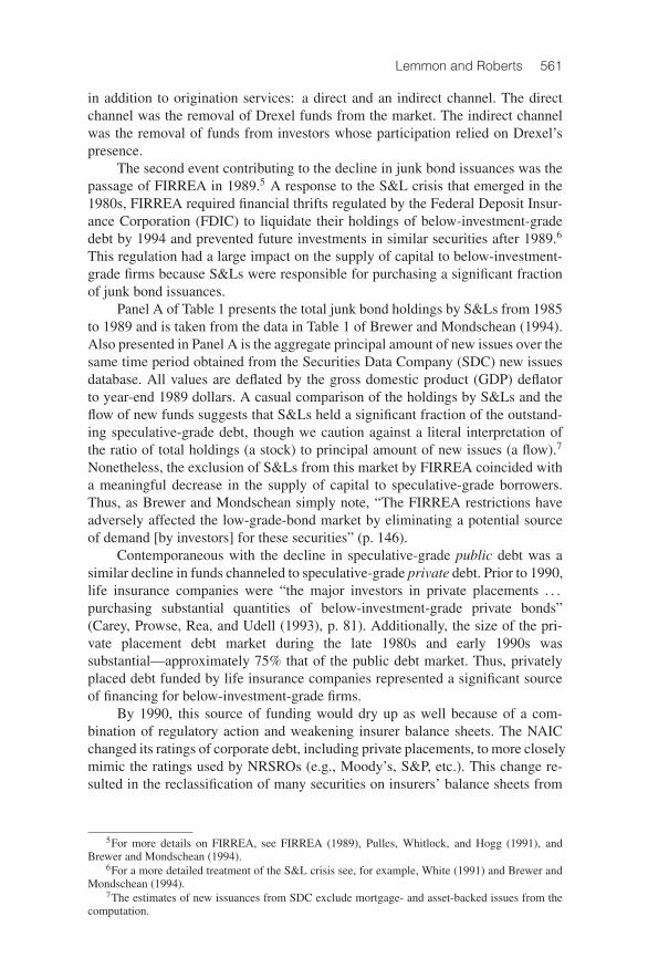
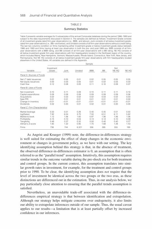
Table 2 presents summary statistics for several groups of firms differentiatedby their rating status during the period 1986–1993. In addition to revealing thegeneral characteristics of our sample of firms, Table 2 is also helpful in identifyingalong which dimensions these groups of firms differ and by how much, albeit ata coarse, aggregate level. Several useful facts emerge. Below-investment-grade(Junk) firms issue relatively more debt (5% of assets) and have a higher leverageratio (50%) than both investment-grade (2% and 30%) and unrated (1% and 26%)firms. Compared to unrated firms, junk firms are 4 times as large and more thantwice as profitable.10 Thus, the greater usage of debt by junk firms is not terriblysurprising given their greater debt capacity, but, more importantly, the use of thisextra debt does not appear to have hampered the financial soundness of junk firmsrelative to their unrated counterparts. A comparison of Altman’s Z-scores showsthat the average junk firm’s Z-score is significantly larger than the average unratedfirm’s Z-score, suggesting that junk firms are, on average, more financially healthythan unrated firms.11
B. Empirical Strategy
As noted above, because the supply shock to the junk bond market was fol-lowed by a recession and changes in the demand for capital, particular care mustbe taken to disentangle the supply and demand effects on corporate behavior. Forexample, a change in the behavior of firms accessing speculative-grade debt after1989 may simply reflect unobserved shifts in these firms’ demand for capital com-mensurate with the change in economic environment. Similarly, a comparison ofjunk bond issuers and, for example, investment-grade bond issuers after 1989 maymerely reflect unmeasured differences between the two groups’ demand for cap-ital. To control for these factors, we employ a difference-in-differences empiricalapproach.
10We focus on market leverage in the presentation of our results. However, in unreported anal-ysis, replacing market leverage with book leverage results in qualitatively similar findings (see theAppendix for the definitions of these variables).
11Altman’s Z-score is a linear combination of sales, income, retained earnings, working capital, andleverage that proxies for the likelihood of financial distress (Altman (1968)). In unreported analysis,we also compare the cash flow volatilities of the three groups, which reveal that junk firms haverelatively lower volatility than unrated firms.
568 Journal of Financial and Quantitative Analysis
TABLE 2
Summary Statistics
Table 2 presents variable averages for 5 subsamples of the annual Compustat database during the period 1986–1993 andsubject to the data requirements discussed in Section II. The samples are defined as follows: Investment Grade consistsof all investment-grade-rated firm-year observations (i.e., BBB– and above), Junk consists of all below-investment-grade-rated firm-year observations (i.e., BB+ and below), and Unrated consists of all firm-year observations without a credit rating.The last two columns condition on firms maintaining either investment-grade or below-investment-grade status between1986 and 1993 and firms having at least one observation in both the pre- and post-1989 era. BBB consists of all firm-year observations with a BBB rating, and BB consists of all firm-year observations with a BB rating. NE HQ consists ofall below-investment-grade firm-year observations with firm headquarters located in the Northeast region of the country,which includes Maine, New Hampshire, Vermont, Massachusetts, Rhode Island, Connecticut, New York, New Jersey, andPennsylvania. Not NE HQ consists of all below-investment-grade firm-year observations with firm headquarters locatedelsewhere in the United States. All variables are defined in the Appendix.
Sample
Investment NotVariable Grade Junk Unrated BBB BB NE HQ NE HQ
Panel A. Sources of Funds
Net LT debt issuances 0.02 0.05 0.01 0.02 0.05 0.05 0.05Net equity issuances 0.00 0.03 0.05 0.01 0.02 0.03 0.03Cash flow 0.12 0.08 0.05 0.11 0.10 0.09 0.07
Panel B. Uses of Funds
Net investment 0.10 0.11 0.09 0.10 0.11 0.11 0.10Capital expenditures 0.08 0.08 0.08 0.09 0.09 0.09 0.06Acquisitions 0.02 0.03 0.02 0.02 0.03 0.02 0.03Sale PPE 0.01 0.01 0.01 0.01 0.01 0.01 0.00Change in inventory –0.01 –0.01 –0.01 –0.01 –0.01 –0.01 –0.01Dividends 0.02 0.00 0.01 0.02 0.01 0.00 0.00
Panel C. Firm Characteristics
Market leverage 0.33 0.51 0.26 0.40 0.45 0.51 0.50log(Sales) 7.82 6.04 3.70 7.50 6.51 6.11 5.82Market-to-book 1.12 1.06 1.60 0.97 1.06 1.06 1.06Profitability 0.15 0.10 0.04 0.13 0.12 0.10 0.09Tangibility 0.48 0.37 0.32 0.50 0.40 0.40 0.27Altman’s Z-score 1.85 1.32 0.95 1.70 1.68 1.28 1.43
Firms 738 744 6,321 356 395 555 189
As Angrist and Krueger (1999) note, the difference-in-differences strategyis well suited for estimating the effect of sharp changes in the economic envi-ronment or changes in government policy, as we have with our setting. The keyidentifying assumption behind this strategy is that, in the absence of treatment,the observed difference-in-differences estimator is 0, an assumption that is oftenreferred to as the “parallel trend” assumption. Intuitively, this assumption requiressimilar trends in the outcome variable during the pre-shock era for both treatmentand control groups. In the current context, this assumption translates into simi-lar growth rates in investment, for example, for the treatment and control groupsprior to 1990. To be clear, the identifying assumption does not require that thelevel of investment be identical across the two groups or the two eras, as thesedistinctions are differenced out in the estimation. Thus, in our analysis below, wepay particularly close attention to ensuring that the parallel trends assumption issatisfied.
Nevertheless, an unavoidable trade-off associated with the difference-in-differences empirical strategy is that between identification and extrapolation.Although our strategy helps mitigate concerns over endogeneity, it also limitsour ability to extrapolate inferences outside of our sample. Thus, the usual caveatapplies to our results—a limitation that is at least partially offset by increasedconfidence in our inferences.

Lemmon and Roberts 569
While our primary interest lies in identifying the effect of the supply shock onnet financing and net investment, we also decompose the financing and investmentvariables into their components. For example, we break out net security issuancesinto long-term debt, short-term debt, and equity. Similarly, net investment is bro-ken out into capital expenditures, acquisitions, and the sale of property, plant, andequipment (PPE).12 Examining each component individually serves three pur-poses. First, it enables us to better understand the precise channels through whichthe supply shock travels. Second, it enables us to quantify the extent of substitu-tion across financing sources. Finally, in conjunction with the aggregate measures,it enables us to examine cross-sectional heterogeneity in financing and investmentbehavior.
V. Results
A. The Impact of the Shock on Below-Investment-Grade Firms
Previous studies examining the supply-side effects on firms’ behaviors haveused a variety of implicit treatment-control comparisons, including: large versussmall firms (Gertler and Gilchrist (1994), Leary (2007)), the presence of a creditrating (Kashyap et al. (1994), Faulkender and Petersen (2006)), and investment-grade versus speculative-grade firms (Sufi (2009)). In this paper, we take a some-what different approach by comparing the behavior of below-investment-gradefirms (the treatment group) with that of a propensity-score-matched sample ofunrated firms (the control group).13
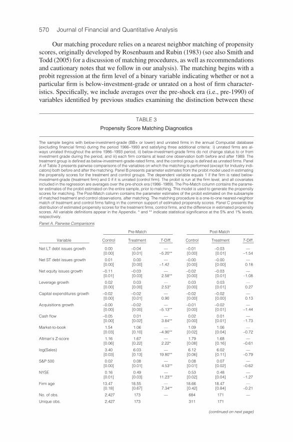
The first 3 columns (Pre-Match) in Panel A of Table 3 illustrate why weundertake a matching approach when comparing these two groups. The columnspresent means, standard errors (in brackets), and t-statistics of the differencesacross the treatment and control groups. As expected, the firms without bondratings are substantially different from firms accessing the speculative-grade debtmarket along a number of dimensions. On average, the firms without bond ratingsare significantly smaller, have higher market-to-book ratios, are less profitable,and are less financially healthy when compared to firms with speculative-gradedebt. In addition, the parallel trends assumption is violated for all of the financingand investment measures with the exception of the growth rates of short-term debtissues and capital expenditures. Thus, a comparison of below-investment-gradefirms to unrated firms as a whole is unlikely to provide an accurate estimate of theimpact of the supply shock on corporate behavior.
12We also examine changes in cash and trade credit; however, unreported results reveal statisti-cally and economically negligible effects of the supply shock on these funding sources in all of ouranalyses. That is, firms are not substituting toward these funds. Similarly, we also examine alterna-tive definitions of net investment incorporating inventory investment, advertising expenditures, andresearch and development (R&D), as well as investment in unconsolidated subsidiaries. The resultsare qualitatively similar to those presented and, therefore, are not reported.
13For an appropriate interpretation of the difference-in-differences estimator, we restrict attentionto firms not transitioning in and out of the treatment and control groups. Thus, we exclude from thepotential control group any firms that were ever rated between 1986 and 1993. Similarly, we excludefrom the treatment group any firms that transition between investment-grade and below-investment-grade between 1986 and 1993. We also require that each firm have at least one observation in thepre-1990 and post-1989 eras in order to compute the within-firm difference.
570 Journal of Financial and Quantitative Analysis
Our matching procedure relies on a nearest neighbor matching of propensityscores, originally developed by Rosenbaum and Rubin (1983) (see also Smith andTodd (2005) for a discussion of matching procedures, as well as recommendationsand cautionary notes that we follow in our analysis). The matching begins with aprobit regression at the firm level of a binary variable indicating whether or not aparticular firm is below-investment-grade or unrated on a host of firm character-istics. Specifically, we include averages over the pre-shock era (i.e., pre-1990) ofvariables identified by previous studies examining the distinction between these
TABLE 3
Propensity Score Matching Diagnostics
The sample begins with below-investment-grade (BB+ or lower) and unrated firms in the annual Compustat database(excluding financial firms) during the period 1986–1993 and satisfying three additional criteria: i) unrated firms are al-ways unrated throughout the entire 1986–1993 period, ii) below-investment-grade firms do not change status to or frominvestment grade during the period, and iii) each firm contains at least one observation both before and after 1989. Thetreatment group is defined as below-investment-grade-rated firms, and the control group is defined as unrated firms. PanelA of Table 3 presents pairwise comparisons of the variables on which the matching is performed (except for Industry indi-cators) both before and after the matching. Panel B presents parameter estimates from the probit model used in estimatingthe propensity scores for the treatment and control groups. The dependent variable equals 1 if the firm is rated below-investment-grade (treatment firm) and 0 if it is unrated (control firm). The probit is run at the firm level, and all covariatesincluded in the regression are averages over the pre-shock era (1986–1989). The Pre-Match column contains the parame-ter estimates of the probit estimated on the entire sample, prior to matching. This model is used to generate the propensityscores for matching. The Post-Match column contains the parameter estimates of the probit estimated on the subsampleof matched treatment and control observations, after matching. The matching procedure is a one-to-one nearest-neighbormatch of treatment and control firms falling in the common support of estimated propensity scores. Panel C presents thedistribution of estimated propensity scores for the treatment firms, control firms, and the difference in estimated propensityscores. All variable definitions appear in the Appendix. * and ** indicate statistical significance at the 5% and 1% levels,respectively.
Panel A. Pairwise Comparisons
Pre-Match Post-Match
Variable Control Treatment T-Diff. Control Treatment T-Diff.
Net LT debt issues growth 0.00 –0.04 — –0.01 –0.03 —[0.00] [0.01] –5.20** [0.00] [0.01] –1.54
Net ST debt issues growth 0.01 0.00 — –0.00 –0.00 —[0.00] [0.00] –1.42 [0.00] [0.00] 0.18
Net equity issues growth –0.11 –0.03 — –0.02 –0.03 —[0.01] [0.03] 2.58** [0.00] [0.01] –1.08
Leverage growth 0.02 0.03 — 0.03 0.03 —[0.00] [0.00] 2.53* [0.00] [0.01] 0.27
Capital expenditures growth –0.02 –0.02 — –0.02 –0.02 —[0.00] [0.01] 0.90 [0.00] [0.00] 0.13
Acquisitions growth –0.00 –0.02 — –0.01 –0.02 —[0.00] [0.00] –5.13** [0.00] [0.01] –1.44
Cash flow –0.05 0.01 — 0.02 0.01 —[0.00] [0.02] 3.84** [0.00] [0.01] –1.73
Market-to-book 1.54 1.06 — 1.09 1.06 —[0.03] [0.10] –4.90** [0.02] [0.04] –0.72
Altman’s Z-score 1.16 1.67 — 1.79 1.68 —[0.06] [0.22] 2.22* [0.08] [0.16] –0.61
log(Sales) 3.40 6.03 — 6.12 6.02 —[0.03] [0.13] 19.80** [0.06] [0.11] –0.79
S&P 500 0.02 0.08 — 0.08 0.07 —[0.00] [0.01] 4.53** [0.01] [0.02] –0.62
NYSE 0.16 0.49 — 0.53 0.48 —[0.01] [0.03] 11.23** [0.02] [0.04] –1.27
Firm age 13.47 18.55 — 18.66 18.47 —[0.18] [0.67] 7.34** [0.42] [0.84] –0.21
No. of obs. 2,427 173 — 684 171 —
Unique obs. 2,427 173 311 171
(continued on next page)

Lemmon and Roberts 571
TABLE 3 (continued)
Propensity Score Matching Diagnostics
Panel B. Probit Regression Results
Pre- Post-Variable Match Match
Intercept –8.85** –0.78*(33.07) (2.40)
Net LT debt issues growth –0.66 –0.21(1.40) (0.45)
Net ST debt issues growth –1.98 0.93(1.30) (0.51)
Net equity issues growth 0.18 –0.20(0.43) (0.31)
Leverage growth 3.60** –0.22(4.54) (0.26)
Capital expenditures growth 0.68 0.42(0.66) (0.39)
Acquisitions growth –1.64* –0.92(2.21) (1.23)
Cash flow 1.06 –1.68(1.51) (1.66)
Market-to-book –0.23** 0.00(2.60) (0.01)
Altman’s Z-score –0.17** 0.02(4.86) (0.49)
log(Sales) 0.51** –0.00(13.08) (0.05)
S&P 500 –0.00 –0.04(0.01) (0.21)
NYSE 0.32** –0.08(2.72) (0.66)
Firm age –0.00 –0.00(0.71) (0.05)
Industry fixed effects Yes Yes
Control 2,427 684Control (unique obs.) 2,427 311Treatment 173 171No. of obs. 2,600 855Pseudo R2 0.37 0.02χ2 p-value 0.00 0.37
Panel C. Estimated Propensity Score Distributions
No. of UniqueObs. Obs. Mean SD Sum Min P5 Median P95 Max
Match Number 1Difference 171 — 0.00 0.00 0.28 0.00 0.00 0.00 0.01 0.02Treatment 171 171 0.30 0.20 51.95 0.00 0.05 0.25 0.72 0.88Control 171 120 0.30 0.20 51.88 0.00 0.05 0.25 0.71 0.87
Match Number 2Difference 171 — 0.00 0.01 0.63 0.00 0.00 0.00 0.02 0.03Treatment 171 171 0.30 0.20 51.95 0.00 0.05 0.25 0.72 0.88Control 171 121 0.30 0.21 51.96 0.00 0.05 0.26 0.74 0.90
Match Number 3Difference 171 — 0.01 0.01 0.93 0.00 0.00 0.00 0.02 0.03Treatment 171 171 0.30 0.20 51.95 0.00 0.05 0.25 0.72 0.88Control 171 128 0.30 0.21 52.05 0.00 0.05 0.26 0.74 0.91
Match Number 4Difference 171 — 0.01 0.01 1.25 0.00 0.00 0.00 0.03 0.05Treatment 171 171 0.30 0.20 51.95 0.00 0.05 0.25 0.72 0.88Control 171 125 0.30 0.20 51.89 0.00 0.05 0.25 0.71 0.84

572 Journal of Financial and Quantitative Analysis
two groups, such as Faulkender and Petersen (2006), as well as other studiesinvestigating the determinants of financing and investment choices (e.g., Titmanand Wessels (1988), Rajan and Zingales (1995), and Eberly, Rebelo, and Vincent(2007)). We incorporate industry indicator variables in an effort to absorb anytime-invariant differences not captured by the firm characteristics.14
We also include several additional controls into the specification to addresstwo concerns. First, we want to ensure that the parallel trends assumption is sat-isfied and, therefore, incorporate growth measures of financing and investmentvariables during the pre-shock era. Second, to address selection concerns overfirms’ decisions to obtain a credit rating, we incorporate the instruments iden-tified by Faulkender and Petersen (2006), who argue that index and exchangelistings, as well as firm age, are valid instruments for identifying financing differ-ences between rated and unrated firms (see Faulkender and Petersen for a detaileddiscussion of this issue).
The probit model is estimated on a cross section of 173 below-investment-grade (treatment) firms and 2,427 unrated (control) firms containing nonmissingdata for all of the variables included in the specification. The estimation resultsare presented in the first column of Panel B in Table 3, labeled “Pre-Match,”and reveal differences that are largely in line with those found in the pairwisecomparison in Panel A. The results also reveal that the specification captures asignificant amount of variation in the choice variable, as indicated by a pseudo-R2
of 37% with a corresponding p-value well below 1%.We then use the predicted probabilities, or propensity scores, from this probit
estimation and perform a nearest-neighbor match with replacement. That is, eachfirm in the treatment group is paired with the firm in the control group whosepropensity score is closest, in an L1-norm sense.15 Because the number of unratedfirms is so large relative to the number of speculative-grade firms (approximately14 times as large), we choose to find 4 control firm matches for each treatmentfirm. We choose 4 matches because it seems to offer the benefit of not relying ontoo little information without incorporating observations that are not sufficientlysimilar. However, we note that changing the number of matches to any numberbetween 1 and 5 has little effect on our results.
Panel C of Table 3 illustrates the accuracy of the matching process by reveal-ing that the majority of differences in the estimated propensity scores betweenthe firms in the treatment group and their corresponding matches from the con-trol group are inconsequential. For the first-best matches (Match Number 1), themaximal difference between the matched propensity scores is 2%, while the 95thpercentile is 1%. Even for the last, or worst, set of matches (Match Number 4), themaximal difference between the treatment and control groups reveals only a 5%difference in propensity scores. The result of the matching process is a treatment
14In estimating the probit, we restrict attention to variables known prior to the supply shock to avoidintroducing any forward-looking bias into the matching process. This ensures that firms are matchedon characteristics that are known prior to the occurrence of the supply shock.
15Following Smith and Todd (2005), we match with replacement to improve the accuracy of thematch, at the cost of lower power. We also require that successful matches fall in the common sup-port of estimated propensity scores. This requirement results in two below-investment-grade firms forwhich we are unable to find a corresponding match.

Lemmon and Roberts 573
group consisting of 171 below-investment-grade firms and a control group con-sisting of the 684 control firms, 311 of which are unique.
The accuracy of the matching process is also shown in the columns denoted“Post-Match” in Panels A and B of Table 3. Specifically, Panel A reveals no sta-tistically significant differences across any of the firm characteristics after thematching process. Similarly, Panel B reveals that none of the determinants arestatistically significant in a probit regression restricted to the matched sample.Further, we note that the magnitudes of the coefficient estimates decline signifi-cantly from the Pre-Match estimation to the Post-Match estimation, ensuring thatour findings are not simply an artifact of a decline in degrees of freedom. (Noneof the industry indicators are statistically significant in the Post-Match probit,though we withhold these findings to ease the presentation of results.) Finally, thepseudo-R2 has fallen from 37% prior to the matching to a statistically insignifi-cant 2% (p-value = 37%) after the matching. In sum, the matching process hasremoved any meaningful differences along observables from the two groups offirms and, in the process, ensured that the parallel trends assumption is satisfied.
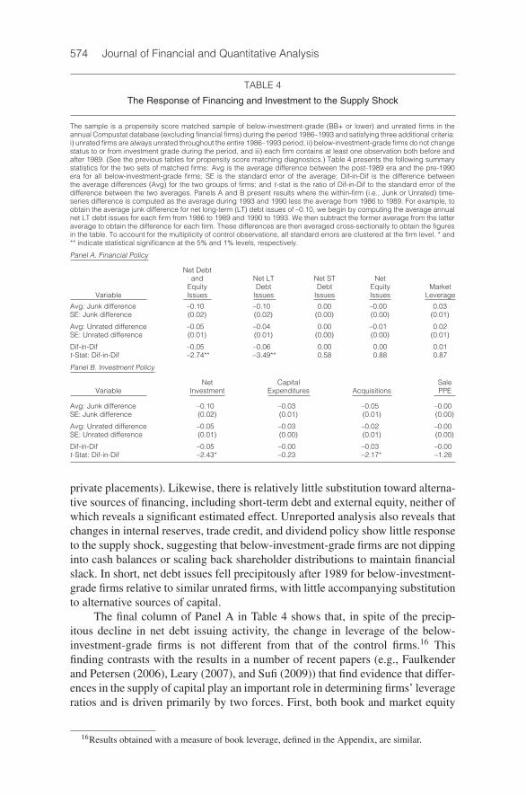
Table 4 presents the results of the difference-in-differences estimation usingthe matched sample. Financial policy variables are presented in Panel A and in-vestment policy variables in Panel B. Each panel presents several summary mea-sures beginning with the average difference between the post-1989 period and thepre-1990 period for the treatment (i.e., Junk) and control (i.e., Matched Unrated)groups. For example, Panel A shows that the average change in net long-term debtissues for below-investment-grade firms is –10% of total assets. This estimate iscomputed by first calculating the average net long-term debt issues from 1990to 1993 and then subtracting the average net long-term debt issues from 1986 to1989 for each firm. This difference is then averaged over below-investment-gradefirms. A similar procedure is performed for the matched unrated firms.
We also present the standard error for each average, suitably adjusted forthe multiple control observations (in parentheses). At the bottom of each panelare the difference-in-differences estimate (Dif-in-Dif) and the corresponding t-statistic of the null hypothesis that this estimate is 0 (t-stat). Note that there isno need for additional control variables since the treatment and control firms arealready matched, nonparametrically, on all of the relevant observable character-istics. We also note that, in unreported analysis, we examine the correspondingmedian values for the treatment and control groups. The results are qualitativelysimilar.
Focusing first on Panel A of Table 4, we see that total net security issuances(net debt plus net equity) by below-investment-grade firms decreased by 5% ofassets relative to the change experienced by similar unrated firms. The averagetotal net security issuances by below-investment-grade firms in our matched sam-ple from 1986 to 1989 is 11%, implying a decline of 45% relative to pre-shocklevels. Thus, aggregate external financing activity contracted sharply for below-investment-grade firms in response to the supply shock.
Columns 2–5 of Panel A in Table 4 reveal that the contraction is concen-trated almost entirely in net long-term debt issuances, indicating that substitutiontoward other forms of debt capital is limited, since this measure encompasses allforms of credit in excess of 1 year in maturity (e.g., public debt, bank debt, and
574 Journal of Financial and Quantitative Analysis
TABLE 4
The Response of Financing and Investment to the Supply Shock
The sample is a propensity score matched sample of below-investment-grade (BB+ or lower) and unrated firms in theannual Compustat database (excluding financial firms) during the period 1986–1993 and satisfying three additional criteria:i) unrated firms are always unrated throughout the entire 1986–1993 period, ii) below-investment-grade firms do not changestatus to or from investment grade during the period, and iii) each firm contains at least one observation both before andafter 1989. (See the previous tables for propensity score matching diagnostics.) Table 4 presents the following summarystatistics for the two sets of matched firms: Avg is the average difference between the post-1989 era and the pre-1990era for all below-investment-grade firms; SE is the standard error of the average; Dif-in-Dif is the difference betweenthe average differences (Avg) for the two groups of firms; and t-stat is the ratio of Dif-in-Dif to the standard error of thedifference between the two averages. Panels A and B present results where the within-firm (i.e., Junk or Unrated) time-series difference is computed as the average during 1993 and 1990 less the average from 1986 to 1989. For example, toobtain the average junk difference for net long-term (LT) debt issues of –0.10, we begin by computing the average annualnet LT debt issues for each firm from 1986 to 1989 and 1990 to 1993. We then subtract the former average from the latteraverage to obtain the difference for each firm. These differences are then averaged cross-sectionally to obtain the figuresin the table. To account for the multiplicity of control observations, all standard errors are clustered at the firm level. * and** indicate statistical significance at the 5% and 1% levels, respectively.
Panel A. Financial Policy
Net Debtand Net LT Net ST Net
Equity Debt Debt Equity MarketVariable Issues Issues Issues Issues Leverage
Avg: Junk difference –0.10 –0.10 0.00 –0.00 0.03SE: Junk difference (0.02) (0.02) (0.00) (0.00) (0.01)
Avg: Unrated difference –0.05 –0.04 0.00 –0.01 0.02SE: Unrated difference (0.01) (0.01) (0.00) (0.00) (0.01)
Dif-in-Dif –0.05 –0.06 0.00 0.00 0.01t-Stat: Dif-in-Dif –2.74** –3.49** 0.58 0.88 0.87
Panel B. Investment Policy
Net Capital SaleVariable Investment Expenditures Acquisitions PPE
Avg: Junk difference –0.10 –0.03 –0.05 –0.00SE: Junk difference (0.02) (0.01) (0.01) (0.00)
Avg: Unrated difference –0.05 –0.03 –0.02 –0.00SE: Unrated difference (0.01) (0.00) (0.01) (0.00)
Dif-in-Dif –0.05 –0.00 –0.03 –0.00t-Stat: Dif-in-Dif –2.43* –0.23 –2.17* –1.28
private placements). Likewise, there is relatively little substitution toward alterna-tive sources of financing, including short-term debt and external equity, neither ofwhich reveals a significant estimated effect. Unreported analysis also reveals thatchanges in internal reserves, trade credit, and dividend policy show little responseto the supply shock, suggesting that below-investment-grade firms are not dippinginto cash balances or scaling back shareholder distributions to maintain financialslack. In short, net debt issues fell precipitously after 1989 for below-investment-grade firms relative to similar unrated firms, with little accompanying substitutionto alternative sources of capital.
The final column of Panel A in Table 4 shows that, in spite of the precip-itous decline in net debt issuing activity, the change in leverage of the below-investment-grade firms is not different from that of the control firms.16 Thisfinding contrasts with the results in a number of recent papers (e.g., Faulkenderand Petersen (2006), Leary (2007), and Sufi (2009)) that find evidence that differ-ences in the supply of capital play an important role in determining firms’ leverageratios and is driven primarily by two forces. First, both book and market equity
16Results obtained with a measure of book leverage, defined in the Appendix, are similar.

Lemmon and Roberts 575
values declined after 1989. Indeed, the decline in equity values was so severethat market leverage actually exhibits a slight increase for both below-investment-grade and unrated firms, separately. Second, as discussed next, investment expe-rienced a contemporaneous contraction limiting asset growth.
Turning to Panel B of Table 4, we see that net investment declined almostone for one with the decline in net debt issuing activity. Net investment by below-investment-grade firms decreased by 5% of assets relative to the change expe-rienced by unrated firms and by approximately 40% relative to the rate of netinvestment prior to the shock. The remaining columns identify the compositionof the investment decline, which is concentrated in slowing acquisition activity(rounding error is the cause of any discrepancy between the aggregate measures,net issuances and net investment, and the sum of their components).17
In sum, our results suggest that the supply contraction in the below-investment-grade debt market had a significant effect on the financing and invest-ment behavior of corresponding firms, though the impact on corporate leverageratios was negligible. These findings illustrate the susceptibility to variations inthe supply of capital of even relatively large firms with access to public debt mar-kets. The following section attempts to buttress this conclusion with additionalevidence from tests of Hypothesis 2, predicting cross-sectional variation in thefinancing and investment response to the supply shock.
B. Cross-Sectional Variation in the Response to the Supply Shock
1. Geographic Heterogeneity in the Cost of Bank Debt
As discussed earlier, the 1990–1991 recession was accompanied by a sharpcontraction in bank lending that was concentrated in the Northeast region of thecountry (Bernanke and Lown (1991), Peek and Rosengren (1995), and Hancockand Wilcox (1998)).18 This localized contraction is primarily attributed to an ero-sion of bank capital driven by declining real estate prices, and therefore this eventis sometimes referred to as a “capital crunch” (Wojnilower (1980), Bernanke andLown, and Peek and Rosengren).
We hypothesize that bank debt is the natural substitute for speculative-gradebonds and assume that the geographic heterogeneity associated with the capi-tal crunch is associated with localized differences in the costs of accessing bankcredit. Below-investment-grade borrowers during this period were effectively re-quired to reintermediate their debt in the absence of below-investment-grade pub-lic debt and private placement investors. Insofar as the geographic location ofcorporate headquarters within the United States is exogenous to the financing de-mand and investment opportunities of firms, we can use location as an instrumentto identify the impact of the loan-supply shock on firm behavior. The assumptionimplicit in this strategy is that firms, on average, tend to borrow from local banks.
17In unreported analysis, we also show that our results are largely immune to concerns of mea-surement error in our proxy for q (Erickson and Whited (2000)), using the reverse regression boundsapproach of Erickson and Whited (2005) to show a sufficiently low correlation between the treatmenteffect variable and our proxy.
18The Northeast region of the United States is comprised of Maine, New Hampshire, Vermont,Massachusetts, Rhode Island, Connecticut, New York, New Jersey, and Pennsylvania.

576 Journal of Financial and Quantitative Analysis
Bharath et al. (2007) confirm this assumption by showing a strong propensity ofpublic firms to borrow from local lenders; however, any deviation from this ten-dency, or noise in this delineation, will tend to attenuate our results.
We define the treatment group as consisting of all below-investment-gradefirms with headquarters located in the Northeast, and the control group as allbelow-investment-grade firms with headquarters located elsewhere in the coun-try. We refer to this sample as the Geography sample. If the availability of substi-tute financing in the form of bank credit was more constrained in the Northeast,then we should observe that below-investment-grade firms located in this regionresponded more severely to the collapse of the junk bond market than did below-investment-grade firms located in other parts of the country.
Table 5 presents results from tests of the parallel trends assumption betweenthe treatment and control groups in the pre-shock period (1986–1989). As seenin the table, the growth in security issuance, both for debt and equity, is statisti-cally identical across the treatment and control groups. Similarly, net investmentgrowth and the growth in market leverage are statistically identical across the twogroups.19 We also note that the magnitudes of the differences, all approximately1% or less, are economically small. Thus, across all of the outcome variables, thetreatment and control groups appear to satisfy the parallel trends assumption.
Estimation of the effects of the supply shock on firm behavior is carried outwith the traditional difference-in-differences regression:
(1) Yit = β0Iit (Post-1989)+β1Iit (NE)+β2Iit(Post-1989)Iit (NE)+γ′Xit−1 +εit,
where i indexes firms, t indexes years, Y is the response variable (e.g., net securityissuances and net investment), I(Post-1989) is an indicator variable equal to 1if the observation occurs after 1989, I(NE) is an indicator variable equal to 1if the firm’s headquarters are located in the Northeast region of the country, Xis a vector of control variables, and ε is the firm-year-specific effect assumedto be correlated within firms and possibly heteroskedastic (Bertrand, Duflo, andMullainathan (2004), Petersen (2009)). The coefficient of interest is β2, whichcorresponds to, approximately, the average change in Y from pre-1989 to post-1989 for the treatment group minus the change in Y from pre-1989 to post-1989for the control group.20
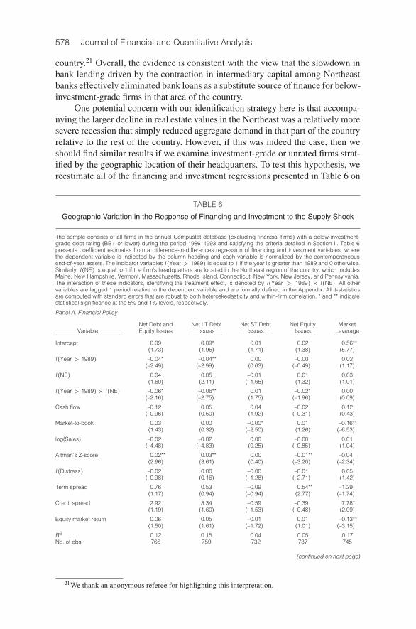
The results from estimating equation (1) are presented in Table 6. While weexamine several variations of the specification in unreported results, we presentonly those results found in the “kitchen-sink” specification incorporating all of
19The growth rate in asset sales reveals a statistically significant difference across the two groups;however, the economic magnitudes are tiny when compared to the other components of net investment.To ensure that our results are not driven by this difference, we examined gross investment, net of theeffect of asset sales. The results are virtually identical to those presented and, consequently, are notreported.
20The relation is only approximate because of possible correlation between the interaction termand X. We also note that the difference-in-differences empirical framework requires us to impose twoadditional data requirements, similar to those found in the propensity score analysis above. First, eachfirm must contain at least one observation in both the pre- and post-1989 periods. Second, we excludethe few firms that change their rating status from below-investment-grade to investment-grade, or viceversa.

Lemmon and Roberts 577
TABLE 5
Tests of Parallel Trends (geography sample)
The sample consists of all firms in the annual Compustat database (excluding financial firms) with a below-investment-grade debt rating (BB+ or lower) during the period 1986–1993 and satisfying three additional criteria: i) each observationssatisfies the data requirements discussed in Section II, ii) the firm does not change status to or from investment grade duringthe period, and iii) the firm contains at least one observation both before and after 1989. Table 5 presents results from testsof the identifying assumption (i.e., parallel trends) behind the difference-in-differences framework by comparing mean (andmedian) annual growth rates (relative to total assets) for each outcome variable during the pre-shock era (1986–1989). Thetreatment group consists of all below-investment-grade-rated firms whose headquarters are located in the Northeast regionof the country, which includes Maine, New Hampshire, Vermont, Massachusetts, Rhode Island, Connecticut, New York,New Jersey, and Pennsylvania. The control groups consists of all below-investment-grade-rated firms whose headquartersare located elsewhere in the United States. The Wilcoxon p-value is the probability value of the two-sample Wilcoxon testof the hypothesis that the two samples are taken from populations with the same median. The t-statistics of the differencein means is presented in parentheses. * and ** indicate statistical significance at the 5% and 1% levels, respectively.
Mean Growth Mean GrowthNot NE HQ NE HQ Wilcoxon
Variable (Control) (Treatment) Difference p-Value
Net debt and equity issues growth –0.05 –0.05 –0.00 0.87(–0.11)
Net LT debt issues growth –0.04 –0.04 0.00 0.97(0.06)
Net ST debt issues growth 0.00 0.00 –0.00 0.40(–0.80)
Net equity issues growth –0.01 –0.01 –0.00 0.65(–0.29)
Net investment growth –0.04 –0.05 0.01 0.70(0.46)
Capital expenditure growth –0.02 –0.01 –0.01 0.66(–1.68)
Acquisition growth –0.02 –0.04 0.01 0.12(1.07)
Sales of assets growth –0.00 0.00 –0.00* 0.36(–2.04)
Market leverage growth 0.04 0.05 –0.01 0.54(–0.52)
the relevant control variables. These estimates are the most conservative in termsof magnitude and statistical significance. Panel A reveals that the net securityissuance activity of below-investment-grade firms in the Northeast part of thecountry experienced a significant decline relative to the change experienced bybelow-investment-grade firms in other parts of the country. Specifically, net secu-rity issuances of firms in the Northeast region fell by 6% of assets relative to firmslocated in other regions. The reduction in security issues is concentrated in long-term debt, and there is no evidence that speculative-grade firms in the Northeastfill the decline in debt issuances with other forms of financing (e.g., short-termdebt, equity, or, in unreported results, changes in cash and trade credit). Interest-ingly, we again find no evidence that the precipitous decline in net debt issuingactivity was accompanied by a significant change in corporate leverage ratios, asrevealed by the last column.
Turning to Panel B of Table 6, we see that net investment fell by 6%, a de-cline concentrated primarily in acquisition activity (4%), as opposed to capitalexpenditures, which fell only modestly (1%). Closer inspection of the coeffi-cients also suggests that the level of debt usage and investment among Northeastfirms in the pre-shock era was slightly higher than among firms elsewhere inthe country. This suggests that one possible interpretation is that the credit con-traction accelerated a return of Northeast firm behavior to that of the rest of the
578 Journal of Financial and Quantitative Analysis
country.21 Overall, the evidence is consistent with the view that the slowdown inbank lending driven by the contraction in intermediary capital among Northeastbanks effectively eliminated bank loans as a substitute source of finance for below-investment-grade firms in that area of the country.
One potential concern with our identification strategy here is that accompa-nying the larger decline in real estate values in the Northeast was a relatively moresevere recession that simply reduced aggregate demand in that part of the countryrelative to the rest of the country. However, if this was indeed the case, then weshould find similar results if we examine investment-grade or unrated firms strat-ified by the geographic location of their headquarters. To test this hypothesis, wereestimate all of the financing and investment regressions presented in Table 6 on
TABLE 6
Geographic Variation in the Response of Financing and Investment to the Supply Shock
The sample consists of all firms in the annual Compustat database (excluding financial firms) with a below-investment-grade debt rating (BB+ or lower) during the period 1986–1993 and satisfying the criteria detailed in Section II. Table 6presents coefficient estimates from a difference-in-differences regression of financing and investment variables, wherethe dependent variable is indicated by the column heading and each variable is normalized by the contemporaneousend-of-year assets. The indicator variables I(Year > 1989) is equal to 1 if the year is greater than 1989 and 0 otherwise.Similarly, I(NE) is equal to 1 if the firm’s headquarters are located in the Northeast region of the country, which includesMaine, New Hampshire, Vermont, Massachusetts, Rhode Island, Connecticut, New York, New Jersey, and Pennsylvania.The interaction of these indicators, identifying the treatment effect, is denoted by I(Year > 1989) × I(NE). All othervariables are lagged 1 period relative to the dependent variable and are formally defined in the Appendix. All t-statisticsare computed with standard errors that are robust to both heteroskedasticity and within-firm correlation. * and ** indicatestatistical significance at the 5% and 1% levels, respectively.
Panel A. Financial Policy
Net Debt and Net LT Debt Net ST Debt Net Equity MarketVariable Equity Issues Issues Issues Issues Leverage
Intercept 0.09 0.09* 0.01 0.02 0.56**(1.73) (1.96) (1.71) (1.38) (5.77)
I(Year > 1989) –0.04* –0.04** 0.00 –0.00 0.02(–2.49) (–2.99) (0.63) (–0.49) (1.17)
I(NE) 0.04 0.05 –0.01 0.01 0.03(1.60) (2.11) (–1.65) (1.32) (1.01)
I(Year > 1989)× I(NE) –0.06* –0.06** 0.01 –0.02* 0.00(–2.16) (–2.75) (1.75) (–1.96) (0.09)
Cash flow –0.12 0.05 0.04 –0.02 0.12(–0.96) (0.50) (1.92) (–0.31) (0.43)
Market-to-book 0.03 0.00 –0.00* 0.01 –0.16**(1.43) (0.32) (–2.50) (1.26) (–6.53)
log(Sales) –0.02 –0.02 0.00 –0.00 0.01(–4.48) (–4.83) (0.25) (–0.85) (1.04)
Altman’s Z-score 0.02** 0.03** 0.00 –0.01** –0.04(2.96) (3.61) (0.40) (–3.20) (–2.34)
I(Distress) –0.02 0.00 –0.00 –0.01 0.05(–0.98) (0.16) (–1.28) (–2.71) (1.42)
Term spread 0.76 0.53 –0.09 0.54** –1.29(1.17) (0.94) (–0.94) (2.77) (–1.74)
Credit spread 2.92 3.34 –0.59 –0.39 7.78*(1.19) (1.60) (–1.53) (–0.48) (2.09)
Equity market return 0.06 0.05 –0.01 0.01 –0.13**(1.50) (1.61) (–1.72) (1.01) (–3.15)
R2 0.12 0.15 0.04 0.05 0.17No. of obs. 766 759 732 737 745
(continued on next page)
21We thank an anonymous referee for highlighting this interpretation.
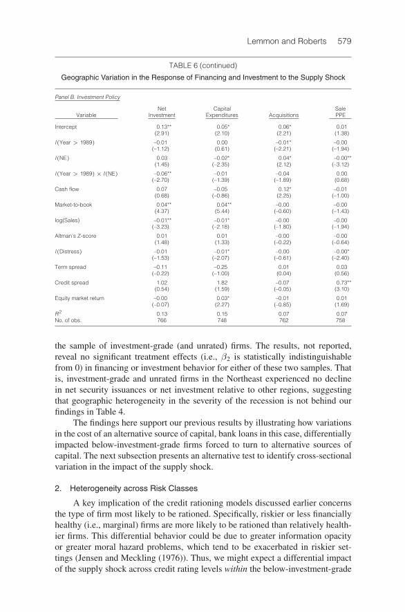
Lemmon and Roberts 579
TABLE 6 (continued)
Geographic Variation in the Response of Financing and Investment to the Supply Shock
Panel B. Investment Policy
Net Capital SaleVariable Investment Expenditures Acquisitions PPE
Intercept 0.13** 0.05* 0.06* 0.01(2.91) (2.10) (2.21) (1.38)
I(Year > 1989) –0.01 0.00 –0.01* –0.00(–1.12) (0.61) (–2.21) (–1.94)
I(NE) 0.03 –0.02* 0.04* –0.00**(1.45) (–2.35) (2.12) (–3.12)
I(Year > 1989)× I(NE) –0.06** –0.01 –0.04 0.00(–2.70) (–1.39) (–1.89) (0.68)
Cash flow 0.07 –0.05 0.12* –0.01(0.68) (–0.86) (2.25) (–1.00)
Market-to-book 0.04** 0.04** –0.00 –0.00(4.37) (5.44) (–0.60) (–1.43)
log(Sales) –0.01** –0.01* –0.00 –0.00(–3.23) (–2.18) (–1.80) (–1.94)
Altman’s Z-score 0.01 0.01 –0.00 –0.00(1.48) (1.33) (–0.22) (–0.64)
I(Distress) –0.01 –0.01* –0.00 –0.00*(–1.53) (–2.07) (–0.61) (–2.40)
Term spread –0.11 –0.25 0.01 0.03(–0.22) (–1.00) (0.04) (0.56)
Credit spread 1.02 1.82 –0.07 0.73**(0.54) (1.59) (–0.05) (3.10)
Equity market return –0.00 0.03* –0.01 0.01(–0.07) (2.27) (–0.85) (1.69)
R2 0.13 0.15 0.07 0.07No. of obs. 766 748 762 758
the sample of investment-grade (and unrated) firms. The results, not reported,reveal no significant treatment effects (i.e., β2 is statistically indistinguishablefrom 0) in financing or investment behavior for either of these two samples. Thatis, investment-grade and unrated firms in the Northeast experienced no declinein net security issuances or net investment relative to other regions, suggestingthat geographic heterogeneity in the severity of the recession is not behind ourfindings in Table 4.
The findings here support our previous results by illustrating how variationsin the cost of an alternative source of capital, bank loans in this case, differentiallyimpacted below-investment-grade firms forced to turn to alternative sources ofcapital. The next subsection presents an alternative test to identify cross-sectionalvariation in the impact of the supply shock.
2. Heterogeneity across Risk Classes
A key implication of the credit rationing models discussed earlier concernsthe type of firm most likely to be rationed. Specifically, riskier or less financiallyhealthy (i.e., marginal) firms are more likely to be rationed than relatively health-ier firms. This differential behavior could be due to greater information opacityor greater moral hazard problems, which tend to be exacerbated in riskier set-tings (Jensen and Meckling (1976)). Thus, we might expect a differential impactof the supply shock across credit rating levels within the below-investment-grade
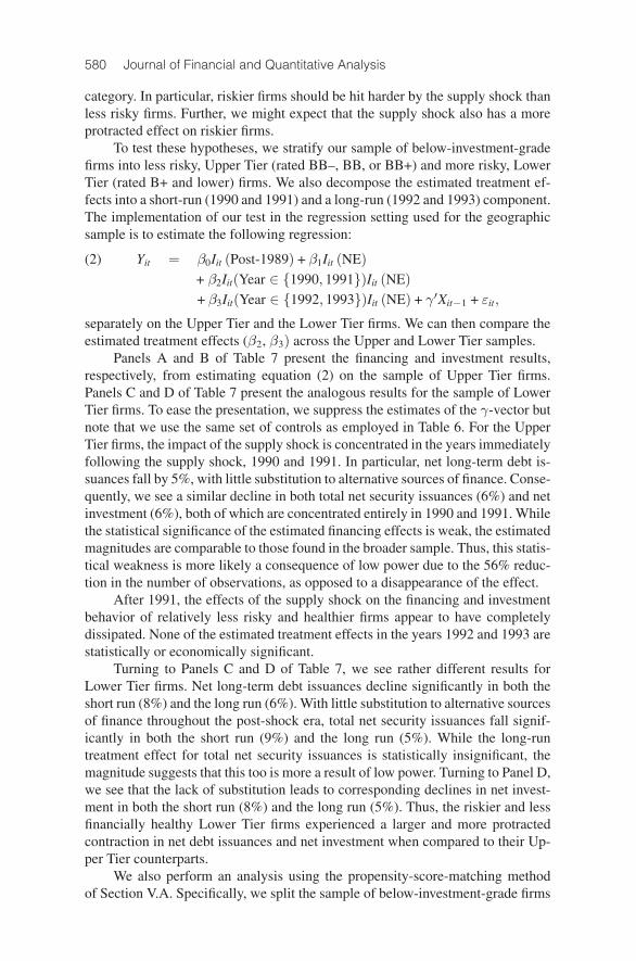
580 Journal of Financial and Quantitative Analysis
category. In particular, riskier firms should be hit harder by the supply shock thanless risky firms. Further, we might expect that the supply shock also has a moreprotracted effect on riskier firms.
To test these hypotheses, we stratify our sample of below-investment-gradefirms into less risky, Upper Tier (rated BB–, BB, or BB+) and more risky, LowerTier (rated B+ and lower) firms. We also decompose the estimated treatment ef-fects into a short-run (1990 and 1991) and a long-run (1992 and 1993) component.The implementation of our test in the regression setting used for the geographicsample is to estimate the following regression:
(2) Yit = β0Iit (Post-1989) + β1Iit (NE)
+ β2Iit(Year ∈ {1990, 1991})Iit (NE)
+ β3Iit(Year ∈ {1992, 1993})Iit (NE) + γ′Xit−1 + εit,
separately on the Upper Tier and the Lower Tier firms. We can then compare theestimated treatment effects (β2, β3) across the Upper and Lower Tier samples.
Panels A and B of Table 7 present the financing and investment results,respectively, from estimating equation (2) on the sample of Upper Tier firms.Panels C and D of Table 7 present the analogous results for the sample of LowerTier firms. To ease the presentation, we suppress the estimates of the γ-vector butnote that we use the same set of controls as employed in Table 6. For the UpperTier firms, the impact of the supply shock is concentrated in the years immediatelyfollowing the supply shock, 1990 and 1991. In particular, net long-term debt is-suances fall by 5%, with little substitution to alternative sources of finance. Conse-quently, we see a similar decline in both total net security issuances (6%) and netinvestment (6%), both of which are concentrated entirely in 1990 and 1991. Whilethe statistical significance of the estimated financing effects is weak, the estimatedmagnitudes are comparable to those found in the broader sample. Thus, this statis-tical weakness is more likely a consequence of low power due to the 56% reduc-tion in the number of observations, as opposed to a disappearance of the effect.
After 1991, the effects of the supply shock on the financing and investmentbehavior of relatively less risky and healthier firms appear to have completelydissipated. None of the estimated treatment effects in the years 1992 and 1993 arestatistically or economically significant.
Turning to Panels C and D of Table 7, we see rather different results forLower Tier firms. Net long-term debt issuances decline significantly in both theshort run (8%) and the long run (6%). With little substitution to alternative sourcesof finance throughout the post-shock era, total net security issuances fall signif-icantly in both the short run (9%) and the long run (5%). While the long-runtreatment effect for total net security issuances is statistically insignificant, themagnitude suggests that this too is more a result of low power. Turning to Panel D,we see that the lack of substitution leads to corresponding declines in net invest-ment in both the short run (8%) and the long run (5%). Thus, the riskier and lessfinancially healthy Lower Tier firms experienced a larger and more protractedcontraction in net debt issuances and net investment when compared to their Up-per Tier counterparts.
We also perform an analysis using the propensity-score-matching methodof Section V.A. Specifically, we split the sample of below-investment-grade firms

Lemmon and Roberts 581
into Upper and Lower Tiers, as defined above, and match each subsample separatelyto unrated firms following the procedure discussed earlier. We then compute twodifference-in-differences estimators corresponding to a short-run (1990–1991)and long-run (1992–1993) effect, as was done with the Geography sample. Be-cause of similar results and space considerations, we merely summarize our find-ings with this analysis, all of which are available from the authors. Specifically,
TABLE 7
Variation in the Response of Financing and Investment to the Supply Shockacross Risk Classes
The sample consists of all firms in the annual Compustat database (excluding financial firms) with a below-investment-grade debt rating (BB+ or lower) during the period 1986–1993 and satisfying the criteria detailed in Section II. Table 7presents coefficient estimates from a difference-in-differences regression of financing and investment variables, where thedependent variable is indicated by the column heading and each variable is normalized by the contemporaneous end-of-year assets. The indicator variable I(Year ∈ {1990, 1991} is equal to 1 if the year is equal to 1990 or 1991 and 0 otherwise(likewise for I(Year ∈ {1992, 1993}). Similarly, I(NE) is equal to 1 if the firm’s headquarters are located in the Northeastregion of the country, which includes Maine, New Hampshire, Vermont, Massachusetts, Rhode Island, Connecticut, NewYork, New Jersey, and Pennsylvania. The interaction of these indicators, identifying the treatment effect, is identified bythe multiplicative term. Other variables included in the regression, but not reported, are: cash flow, market-to-book ratio,log(sales), Altman’s Z-score, a financial distress indicator, a measure of the term spread, a measure of the credit spread,and the firms’ annual equity return. All of these variables are lagged 1 period relative to the dependent variable and areformally defined in the Appendix. Panels A and B present the financing and investment results for Upper Tier firms, ratedBB–, BB, or BB+, respectively. Panels C and D present the financing and investment results for Lower Tier firms, ratedB+ or lower, respectively. All t-statistics are computed with standard errors that are robust to both heteroskedasticity andwithin-firm correlation. * and ** indicate statistical significance at the 5% and 1% levels, respectively.
Panel A. Financial Policy—Upper Tier Firms (rated BB–, BB, or BB+)
NetDebt Net Netand LT ST Net
Equity Debt Debt Equity MarketVariable Issues Issues Issues Issues Leverage
Intercept 0.06 –0.00 0.02 0.03 0.25*(0.55) (–0.04) (1.83) (0.92) (2.19)
I(Year > 1989) –0.05* –0.06** 0.00 –0.00 –0.01(–2.52) (–2.85) (0.56) (–0.18) (–0.27)
I(NE) 0.02 0.01 –0.00 0.02 0.03(0.65) (0.42) (–0.25) (1.73) (–0.70)
I(Year ∈ {1990, 1991})× I(NE) –0.06 –0.05 0.00 –0.02 –0.00(–1.61) (–1.40) (0.44) (–0.95) (–0.04)
I(Year ∈ {1992, 1993})× I(NE) 0.01 –0.00 0.01 –0.00 0.00(0.26) (–0.11) (1.10) (–0.06) (0.04)
Additional control variables Yes Yes Yes Yes Yes
R2 0.14 0.18 0.05 0.11 0.23No. of obs. 334 332 321 321 333
Panel B. Investment Policy—Upper Tier Firms (rated BB–, BB, or BB+)
Net Capital SaleVariable Investment Expenditures Acquisitions PPE
Intercept 0.05 0.03 0.03 –0.00(0.89) (0.93) (0.75) (–0.61)
I(Year > 1989) –0.01 –0.00 –0.01 –0.00(–0.70) (–0.22) (–0.73) (–0.95)
I(NE) 0.01 –0.02* 0.03 –0.00*(0.49) (–2.31) (1.37) (–1.99)
I(Year ∈ {1990, 1991})× I(NE) –0.06** –0.01 –0.05* 0.00(–2.73) (–0.95) (–2.17) (0.42)
I(Year ∈ {1992, 1993})× I(NE) 0.01 –0.02 0.02 0.00(0.13) (–1.21) (0.48) (0.58)
Additional control variables Yes Yes Yes Yes
R2 0.17 0.18 0.10 0.04No. of obs. 334 326 332 329
(continued on next page)
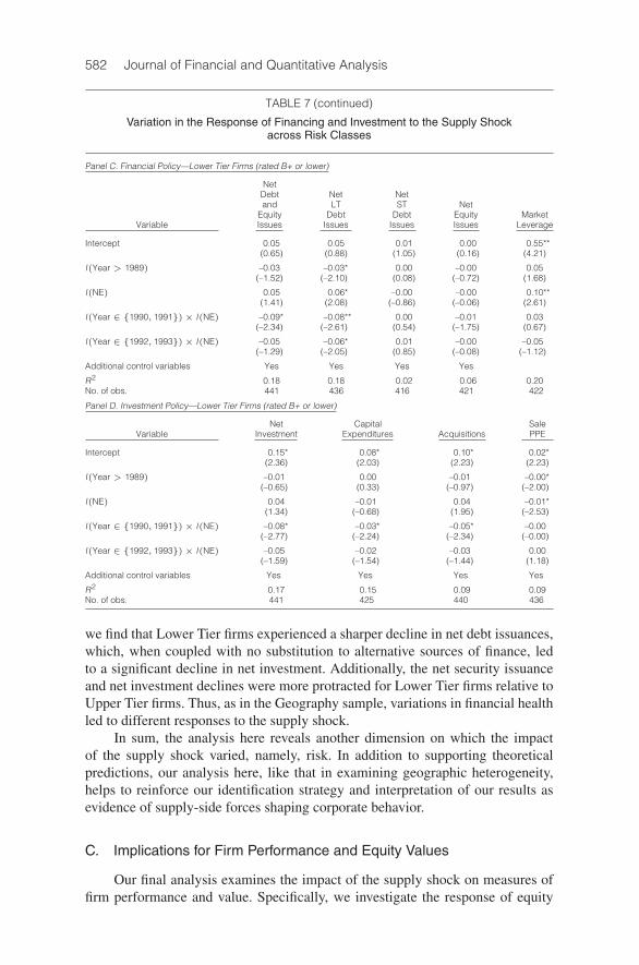
582 Journal of Financial and Quantitative Analysis
TABLE 7 (continued)
Variation in the Response of Financing and Investment to the Supply Shockacross Risk Classes
Panel C. Financial Policy—Lower Tier Firms (rated B+ or lower)
NetDebt Net Netand LT ST Net
Equity Debt Debt Equity MarketVariable Issues Issues Issues Issues Leverage
Intercept 0.05 0.05 0.01 0.00 0.55**(0.65) (0.88) (1.05) (0.16) (4.21)
I(Year > 1989) –0.03 –0.03* 0.00 –0.00 0.05(–1.52) (–2.10) (0.08) (–0.72) (1.68)
I(NE) 0.05 0.06* –0.00 –0.00 0.10**(1.41) (2.08) (–0.86) (–0.06) (2.61)
I(Year ∈ {1990, 1991})× I(NE) –0.09* –0.08** 0.00 –0.01 0.03(–2.34) (–2.61) (0.54) (–1.75) (0.67)
I(Year ∈ {1992, 1993})× I(NE) –0.05 –0.06* 0.01 –0.00 –0.05(–1.29) (–2.05) (0.85) (–0.08) (–1.12)
Additional control variables Yes Yes Yes Yes
R2 0.18 0.18 0.02 0.06 0.20No. of obs. 441 436 416 421 422
Panel D. Investment Policy—Lower Tier Firms (rated B+ or lower)
Net Capital SaleVariable Investment Expenditures Acquisitions PPE
Intercept 0.15* 0.08* 0.10* 0.02*(2.36) (2.03) (2.23) (2.23)
I(Year > 1989) –0.01 0.00 –0.01 –0.00*(–0.65) (0.33) (–0.97) (–2.00)
I(NE) 0.04 –0.01 0.04 –0.01*(1.34) (–0.68) (1.95) (–2.53)
I(Year ∈ {1990, 1991})× I(NE) –0.08* –0.03* –0.05* –0.00(–2.77) (–2.24) (–2.34) (–0.00)
I(Year ∈ {1992, 1993})× I(NE) –0.05 –0.02 –0.03 0.00(–1.59) (–1.54) (–1.44) (1.18)
Additional control variables Yes Yes Yes Yes
R2 0.17 0.15 0.09 0.09No. of obs. 441 425 440 436
we find that Lower Tier firms experienced a sharper decline in net debt issuances,which, when coupled with no substitution to alternative sources of finance, ledto a significant decline in net investment. Additionally, the net security issuanceand net investment declines were more protracted for Lower Tier firms relative toUpper Tier firms. Thus, as in the Geography sample, variations in financial healthled to different responses to the supply shock.
In sum, the analysis here reveals another dimension on which the impactof the supply shock varied, namely, risk. In addition to supporting theoreticalpredictions, our analysis here, like that in examining geographic heterogeneity,helps to reinforce our identification strategy and interpretation of our results asevidence of supply-side forces shaping corporate behavior.
C. Implications for Firm Performance and Equity Values
Our final analysis examines the impact of the supply shock on measures offirm performance and value. Specifically, we investigate the response of equity
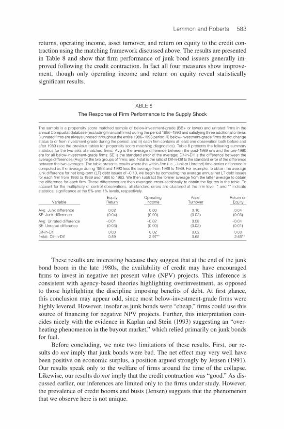
Lemmon and Roberts 583
returns, operating income, asset turnover, and return on equity to the credit con-traction using the matching framework discussed above. The results are presentedin Table 8 and show that firm performance of junk bond issuers generally im-proved following the credit contraction. In fact all four measures show improve-ment, though only operating income and return on equity reveal statisticallysignificant results.
TABLE 8
The Response of Firm Performance to the Supply Shock
The sample is a propensity score matched sample of below-investment-grade (BB+ or lower) and unrated firms in theannual Compustat database (excluding financial firms) during the period 1986–1993 and satisfying three additional criteria:i) unrated firms are always unrated throughout the entire 1986–1993 period, ii) below-investment-grade firms do not changestatus to or from investment grade during the period, and iii) each firm contains at least one observation both before andafter 1989 (see the previous tables for propensity score matching diagnostics). Table 8 presents the following summarystatistics for the two sets of matched firms: Avg is the average difference between the post-1989 era and the pre-1990era for all below-investment-grade firms; SE is the standard error of the average; Dif-in-Dif is the difference between theaverage differences (Avg) for the two groups of firms; and t-stat is the ratio of Dif-in-Dif to the standard error of the differencebetween the two averages. The table presents results where the within-firm (i.e., Junk or Unrated) time-series difference iscomputed as the average during 1993 and 1990 less the average from 1986 to 1989. For example, to obtain the averagejunk difference for net long-term (LT) debt issues of –0.10, we begin by computing the average annual net LT debt issuesfor each firm from 1986 to 1989 and 1990 to 1993. We then subtract the former average from the latter average to obtainthe difference for each firm. These differences are then averaged cross-sectionally to obtain the figures in the table. Toaccount for the multiplicity of control observations, all standard errors are clustered at the firm level. * and ** indicatestatistical significance at the 5% and 1% levels, respectively.
Equity Operating Asset Return onVariable Return Income Turnover Equity
Avg: Junk difference 0.02 0.00 0.10 0.04SE: Junk difference (0.04) (0.00) (0.02) (0.03)
Avg: Unrated difference –0.01 –0.02 0.08 –0.04SE: Unrated difference (0.03) (0.00) (0.02) (0.01)
Dif-in-Dif 0.03 0.02 0.02 0.08t-stat: Dif-in-Dif 0.59 2.97** 0.68 2.65**
These results are interesting because they suggest that at the end of the junkbond boom in the late 1980s, the availability of credit may have encouragedfirms to invest in negative net present value (NPV) projects. This inference isconsistent with agency-based theories highlighting overinvestment, as opposedto those highlighting the discipline imposing benefits of debt. At first glance,this conclusion may appear odd, since most below-investment-grade firms werehighly levered. However, insofar as junk bonds were “cheap,” firms could use thissource of financing for negative NPV projects. Further, this interpretation coin-cides nicely with the evidence in Kaplan and Stein (1993) suggesting an “over-heating phenomenon in the buyout market,” which relied primarily on junk bondsfor fuel.
Before concluding, we note two limitations of these results. First, our re-sults do not imply that junk bonds were bad. The net effect may very well havebeen positive on economic surplus, a position argued strongly by Jensen (1991).Our results speak only to the welfare of firms around the time of the collapse.Likewise, our results do not imply that the credit contraction was “good.” As dis-cussed earlier, our inferences are limited only to the firms under study. However,the prevalence of credit booms and busts (Jensen) suggests that the phenomenonthat we observe here is not unique.

584 Journal of Financial and Quantitative Analysis
VI. Conclusion
We use the shock to the supply of below-investment-grade debt precipitatedby the fall of Drexel, the enactment of FIRREA, and changes in the insurance in-dustry in late 1989 to early 1990 to examine the impact of fluctuations in the sup-ply of capital on the distribution of financing and investment. The specificity andexogenous nature of these events enable us to employ a difference-in-differencesresearch design aimed at disentangling supply-side from demand-side forces.
Our results show that the contraction in the supply of credit to below-investment-grade firms significantly altered their financing and investment behav-ior. Net debt issuances were nearly halved relative to what they were prior to thesupply shock. This contraction was accompanied by almost no substitution to al-ternative sources of finance, such as bank debt, equity, retained earnings, or tradecredit. Consequently, net investment declined almost one for one with the declinein net debt issuances. The contemporaneous decline in debt and investment hadoffsetting effects on corporate leverage ratios, which were largely unaffected bythe supply shock.
While the events contributing to the contraction in credit supply after 1989were unique—enabling identification of the supply effect—one cannot help butdraw parallels between the influx of money into the high-yield market in the 1980sand the influx of money into venture capital in the late 1990s and, especially, thehigh-yield market today. Whether today’s speculative-grade firms will experienceoutcomes similar to those of their predecessors remains to be seen. As such, welook forward to future research that examines the impact of this and other sup-ply effects on corporate behavior, as well as research aimed at uncovering theunderlying mechanisms linking supply-side forces to corporate behavior.
Appendix. Variable Definitions
All numbers in parentheses refer to annual Compustat item numbers.
Credit Rating = senior long-term debt rating (280).
Net Investment = (capital expenditures (128) + acquisitions (129) – sale PPE (107) + in-crease in investments (219) – sale of investments (109)) ÷ start-of-period assets (6).
Net LT Debt Issues = long-term debt issues (111) – long-term debt reduction (114) ÷start-of-period assets.
Net ST Debt Issues = change in current debt (301) ÷ start-of-period assets.
Net Equity Issues = sale of common and preferred stock (108) – purchase of common andpreferred stock (115) ÷ start-of-period assets.
Net Issues of Secured Debt and Mortgages = change in secured debt and mortgages (241)÷ start-of-period assets.
Change in Trade Credit = change in accounts payable (304) + change in accounts receivable(302) ÷ start-of-period assets.
Change in Cash = change in cash equivalents (274) ÷ start-of-period assets.
Total Debt = long-term debt (9) + short-term debt (34).
Book Leverage = total debt ÷ book assets (6).

Lemmon and Roberts 585
Market Value of Assets = stock Price (199) × shares outstanding (25) + short-term debt +long-term debt + preferred stock liquidation value (10) – deferred taxes and investment taxcredits (35).
Market Leverage = total debt ÷ market value of assets.
Firm Size = log(sales), where sales (12) are deflated by the GDP deflator.
Market-to-Book = (market equity + total debt + preferred stock liquidating value – deferredtaxes and investment tax credits) ÷ book assets.
Z-Score = 3.3 × pre-tax income (170) + sales (12) + 1.4 × retained earnings (36) + 1.2 ×(current assets (4) – current liabilities (5)) ÷ book assets.
Cash Flow = income before extraordinary items (123) ÷ lagged book assets.
Net Equity Issues (Alternative) = the split-adjusted change in shares outstanding (data25t−data25t−1 × (data27t−1 ÷ data27t) × the split-adjusted average stock price (data199t +data199t−1 × (data27t ÷ data27t−1)÷ the end-of-year t − 1 total assets.
Financially Distressed = indicator variable equal to 1 if either i) the firm’s earnings beforeinterest, taxes, depreciation, and amortization (EBITDA) is less than its reported interestexpense for the previous 2 years or, ii) EBITDA is less than 80% of its interest expense inthe previous year.
Term Spread = the yield spread between the 1- and 10-year Treasury bonds.
Credit Spread = the yield spread between BB– and BBB-rated corporate bonds.
Equity Market Return = CRSP annual value-weighted return.
S&P 500 = indicator equal to 1 if the firm is in the S&P 500 index.
NYSE = indicator equal to 1 if the firm is listed on the NYSE.
Firm Age = the age of the firm computed as the number of years in which the firm has beenlisted on Compustat and has a nonmissing value for total assets.
Operating Income = operating income (data13) before depreciation ÷ total assets.
Asset Turnover = total sales (data12) ÷ total assets.
Return on Equity = operating income before depreciation ÷ book equity (data60).
ReferencesAltman, E. I. “Financial Ratios, Discriminant Analysis, and the Prediction of Corporate Bankruptcy.”
Journal of Finance, 23 (1968), 589–609.Angrist, J. D., and A. B. Krueger. “Empirical Strategies in Labor Economics.” Handbook of Labor
Economics, Vol. 3A, O. Ashenfelter and D. Card, eds. Amsterdam, The Netherlands: ElsevierScience (1999).
Asquith, P.; D. W. Mullins; and E. D. Wolff. “Original Issue High Yield Bonds: Aging Analyses ofDefaults, Exchanges, and Calls.” Journal of Finance, 44 (1989), 923–952.
Benston, G. J., and G. G. Kaufman. “FDICIA after Five Years.” Journal of Economic Perspectives, 11(1997), 139–158.
Benveniste, L. M.; M. Singh; and W. J. Wilhelm, Jr. “The Failure of Drexel Burnham Lambert: Evi-dence on the Implications for Commercial Banks.” Journal of Financial Intermediation, 3 (1993),104–137.
Berger, A. N., and G. F. Udell. “Relationship Lending and Lines of Credit Small Firm Finance.”Journal of Business, 68 (1995), 351–381.
Bernanke, B. S.; J. Y. Campbell; and T. M. Whited. “U.S. Corporate Leverage: Developments in 1987and 1988.” Brookings Papers on Economic Activity (1990), 255–278.
Bernanke, B. S., and M. Gertler. “Agency Costs, Net Worth and Business Fluctuations.” AmericanEconomic Review, 79 (1989), 14–31.

586 Journal of Financial and Quantitative Analysis
Bernanke, B. S., and C. S. Lown. “The Credit Crunch.” Brookings Papers on Economic Activity (1991),205–247.
Bertrand, M.; E. Duflo; and S. Mullainathan. “How Much Should We Trust Differences-in-DifferencesEstimates?” Quarterly Journal of Economics, 119 (2004), 249–275.
Bharath, S.; S. Dahiya; A. Saunders; and A. Srinivasan. “So What Do I Get? The Bank’s View ofLending Relationships.” Journal of Financial Economics, 85 (2007) 368–419.
Bolton, P., and X. Freixas. “Equity, Bonds, and Bank Debt: Capital Structure and Financial MarketEquilibrium under Asymmetric Information.” Journal of Political Economy, 108 (2000), 324–351.
Bolton, P., and D. Scharfstein. “Optimal Debt Structure with Multiple Creditors.” Journal of PoliticalEconomy, 104 (1996), 1–26.
Brewer, E., and T. H. Mondschean. “An Empirical Test of the Incentive Effects of Deposit Insur-ance: The Case of Junk Bonds at Savings and Loan Associations.” Journal of Money, Credit, andBanking, 26 (1994), 146–164.
Carey, M. S.; S. D. Prowse; J. D. Rea; and G. F. Udell. “Recent Developments in the Market forPrivately Placed Debt.” Federal Reserve Bulletin, 79 (1993), 77–92.
Chava, S., and A. K. Purnanandam. “The Effect of Banking Crisis on Bank-Dependent Borrowers.”Working Paper, University of Michigan (2006).
Diamond, D. W. “Financial Intermediation and Delegated Monitoring.” Review of Economic Studies,51 (1984), 393–414.
Diamond, D. W. “Monitoring and Reputation: The Choice between Bank Loans and Directly PlacedDebt.” Journal of Political Economy, 99 (1991), 688–721.
Diamond, D. W. “Corporate Capital Structure: The Control Roles of Bank and Public Debt with Taxesand Costly Bankruptcy.” Economic Quarterly—Federal Reserve Bank of Richmond, 80 (1994),11–37.
Eberly, J. C.; S. T. Rebelo; and N. Vincent. “Investment and Value: A Neoclassical Benchmark.”Working Paper, Northwestern University (2007).
Erickson, T., and T. M. Whited. “Measurement Error and the Relationship between Investment and‘q’.” Journal of Political Economy, 108 (2000), 1027–1057.
Erickson, T., and T. M. Whited. “Proxy-Quality Thresholds: Theory and Applications.” Finance Re-search Letters, 2 (2005), 131–151.
Fama, E. F. “What’s Different about Banks?” Journal of Monetary Economics, 15 (1985), 29–39.Faulkender, M., and M. A. Petersen. “Does the Source of Capital Affect Capital Structure?” Review
of Financial Studies, 19 (2006), 45–79.Financial Institutions Reform, Recovery & Enforcement Act of 1989 (9 vols.). Chicago, IL: United
States League of Savings Institutions (1989).Gertler, M., and S. Gilchrist. “Monetary Policy, Business Cycles, and the Behavior of Small Manu-
facturing Firms.” Quarterly Journal of Economics, 109 (1994), 309–340.Graham, J. R., and C. R. Harvey. “The Theory and Practice of Corporate Finance: Evidence from the
Field.” Journal of Financial Economics, 60 (2001), 187–243.Hancock, D., and J. A. Wilcox. “The ‘Credit Crunch’ and the Availability of Credit to Small Business.”
Journal of Banking and Finance, 22 (1998), 983–1014.Hart, O., and J. Moore. “Debt and Seniority: An Analysis of the Role of Hard Claims in Constraining
Management.” American Economic Review, 85 (1995), 567–585.He, Z., and A. Krishnamurthy. “Intermediation, Capital Immobility, and Asset Prices.” Working Paper,
Northwestern University (2006).Holmstrom, B., and S. N. Kaplan. “Corporate Governance and Merger Activity in the United States:
Making Sense of the 1980s and 1990s.” Journal of Economic Perspectives, 15 (2001), 121–144.Holmstrom, B., and J. Tirole. “Financial Intermediation, Loanable Funds, and the Real Sector.” Quar-
terly Journal of Economics, 112 (1997), 663–691.Jaffee, D. M., and T. Russell. “Imperfect Information, Uncertainty, and Credit Rationing.” Quarterly
Journal of Economics, 90 (1976), 651–666.Jensen, M. C. “Corporate Control and the Politics of Finance.” Journal of Applied Corporate Finance,
4 (1991), 13–33.Jensen, M. C., and W. H. Meckling. “Theory of the Firm: Managerial Behavior, Agency Costs and
Ownership Structure.” Journal of Financial Economics, 3 (1976), 305–360.Kaplan, S. N., and J. C. Stein. “The Evolution of Buyout Pricing and Financial Structure in the 1980s.”
Quarterly Journal of Economics, 108 (1993), 313–357.Kashyap, A. K.; O. A. Lamont; and J. C. Stein. “Credit Conditions and the Cyclical Behavior of
Inventories.” Quarterly Journal of Economics, 109 (1994), 565–592.Kashyap, A. K.; J. C. Stein; and D. W. Wilcox. “Monetary Policy and Credit Conditions: Evidence
from the Composition of External Finance.” American Economic Review, 83 (1993), 78–98.Kisgen, D. J. “Credit Ratings and Capital Structure.” Journal of Finance, 61 (2006), 1035–1072.

Lemmon and Roberts 587
Leary, M. T. “Bank Loan Supply, Lender Choice, and Corporate Capital Structure.” Working Paper,Cornell University (2007).
Modigliani, F., and M. H. Miller. “The Cost of Capital, Corporation Finance and the Theory of Invest-ment.” American Economic Review, 48 (1958), 261–297.
Myers, S. C., and N. S. Majluf. “Corporate Financing and Investment Decisions When Firms HaveInformation That Investors Do Not Have.” Journal of Financial Economics, 13 (1984), 187–221.
Oliner, S. D., and G. D. Rudebusch. “Monetary Policy and Credit Conditions: Evidence from theComposition of External Finance: Comment.” American Economic Review, 86 (1996), 300–309.
Peek, J., and E. Rosengren. “The Capital Crunch: Neither a Borrower nor a Lender Be.” Journal ofMoney, Credit, and Banking, 27 (1995), 625–638.
Petersen, M. A. “Estimating Standard Errors in Finance Panel Data Sets: Comparing Approaches.”Review of Financial Studies, 22 (2009), 435–480.
Petersen, M. A., and R. G. Rajan. “The Effect of Credit Market Competition on Lending Relation-ships.” Quarterly Journal of Economics, 110 (1995), 407–443.
Pontell, H. N., and K. Calavita. “The Savings and Loan Industry.” Crime and Justice, 18 (1993),203–246.
Pulles, G.; R. Whitlock; and J. Hogg. “FIRREA: A Legislative History and Section-by-Section Anal-ysis of the Financial Institutions Recovery, Reform, and Enforcement Act.” Colorado Springs, CO:Shepard’s/McGraw-Hill, Inc. (1991).
Rajan, R. G. “Insiders and Outsiders: The Choice between Informed and Arm’s-Length Debt.” Journalof Finance, 47 (1992), 1367–1400.
Rajan, R. G., and L. Zingales. “What Do We Know about Capital Structure? Some Evidence fromInternational Data.” Journal of Finance, 50 (1995), 1421–1460.
Rosenbaum, P. R., and D. B. Rubin. “The Central Role of the Propensity Score in ObservationalStudies for Causal Effects.” Biometrika, 70 (1983), 41–55.
Simonson, M. “The Fall of Drexel Burnham Lambert and the Value of Its Junk Bond-Issuing Clients.”Working Paper, Arizona State University (2000).
Smith, J. A., and P. E. Todd. “Does Matching Overcome LaLonde’s Critique of NonexperimentalEstimators?” Journal of Econometrics, 125 (2005), 305–353.
Standard & Poor’s. Corporate Ratings Criteria. New York, NY: McGraw-Hill (2001).Stiglitz, J. E., and A. Weiss. “Credit Rationing in Markets with Imperfect Information.” American
Economic Review, 71 (1981), 393–410.Sufi, A. “The Real Effects of Debt Certification: Evidence from the Introduction of Bank Loan Rat-
ings.” Review of Financial Studies, 22 (2009), 1659–1691.Titman, S. “The Modigliani and Miller Theorem and Market Efficiency.” NBER Working Paper 8641
(2001).Titman, S., and R. Wessels. “The Determinants of Capital Structure Choice.” Journal of Finance, 43
(1988) 1–19.White, L. J. The S&L Debacle: Public Policy Lessons for Bank and Thrift Regulation. New York, NY:
Oxford University Press (1991).Wojnilower, A. M. “The Central Role of Credit Crunches in Recent Financial History.” Brookings
Papers on Economic Activity (1980), 277–326.Zarutskie, R. “Evidence on the Effects of Bank Competition on Firm Borrowing and Investment.”
Journal of Financial Economics, 81 (2006), 503–537.