THE REMEZ ALGORITHM - NYU Tandon School of …eeweb.poly.edu/iselesni/EL713/remez/remez.pdf · the value is taken as a variable in this interpolation problem, so ... is not always

THE REMEZ ALGORITHM

This section describes how to design linear-phase FIR filters based

on the Chebyshev (or minimax) error criterion. The minimization

of the Chebyshev norm is useful because it permits the user to ex-

plicitly specify band-edges and relative error sizes in each band. We

will see that linear-phase FIR filters that minimize a Chebyshev er-

ror criterion can be found with the Remez algorithm or by linear

programming techniques. Both these methods are iterative numer-

ical algorithms and can be used for very general functions D(ω)

and W (ω) (although many implementations work only for piece-

wise linear functions). The Remez algorithm is not as general as

the linear programming approach, but it is very robust, converges

very rapidly to the optimal solution, and is widely used.

I. Selesnick EL 713 Lecture Notes 1

THE PARKS-McCLELLAN ALGORITHM

Parks and McClellan proposed the use of the Remez algorithm for

FIR filter design and made programs available [5, 6, 9, 15]. Many

texts describe the Parks-McClellan (PM) algorithm in detail [7, 8,

11, 14].

The Remez algorithm can be use to design all four types of linear-

phase filters (I,II,III,IV), but for convenience only the design of type

I filters will be described here. Note that the weighted error function

is given by

E(ω) = W (ω) (A(ω)−D(ω)). (1)

The amplitude response of a type I FIR filter is given by

A(ω) =M∑n=0

a(n) cos(nω). (2)


PROBLEM FORMULATION

The Chebyshev design problem can formulated as follows. Given:

N : filter length

D(ω) : desired (real-valued) amplitude function

W (ω) : nonnegative weighting function,

find the linear-phase filter that minimizes the weighted Chebyshev

error, defined by

||E(ω)||∞ = maxω∈[0,π]

|W (ω) (A(ω)−D(ω))|. (3)

The solution to this problem is called the best weighted Chebyshev

approximation to D(ω). Because it minimizes the maximum value

of the error, it is also called the minimax solution.

The Remez algorithm for computing the best Chebyshev solution

uses the alternation theorem. This theorem characterizes the best

Chebyshev solution.


LOW-PASS CHEBYSHEV FILTERS

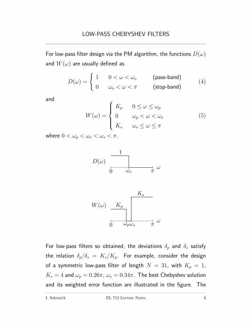
For low-pass filter design via the PM algorithm, the functions D(ω)

and W (ω) are usually defined as

D(ω) =

{1 0 < ω < ωo (pass-band)

0 ωo < ω < π (stop-band)(4)

and

W (ω) =

Kp 0 ≤ ω ≤ ωp

0 ωp < ω < ωs

Ks ωs ≤ ω ≤ π

(5)

where 0 < ωp < ωo < ωs < π.

ωD(ω)

0 ωo π

1

ω

W (ω)

0 ωpωs π

Kp

Ks

For low-pass filters so obtained, the deviations δp and δs satisfy

the relation δp/δs = Ks/Kp. For example, consider the design

of a symmetric low-pass filter of length N = 31, with Kp = 1,

Ks = 4 and ωp = 0.26π, ωs = 0.34π. The best Chebyshev solution

and its weighted error function are illustrated in the figure. The


maximum errors in the pass-band and stop-band are δp = 0.0892

and δs = 0.0223 respectively. The circular marks in the figure

indicate the extremal points of the alternation theorem.

0 0.2 0.4 0.6 0.8 1−0.2

0

0.2

0.4

0.6

0.8

1

ω/π

A(ω

)

0 0.2 0.4 0.6 0.8 1−0.1

−0.05

0

0.05

0.1

ω/π

W(ω

) (A

(ω)−

D(ω

))

0 0.2 0.4 0.6 0.8 1−60

−50

−40

−30

−20

−10

0

10

ω/π

|A(ω

)|,

in d

B

0 10 20 30−0.1

0

0.1

0.2

0.3

n

h(n

)


ALTERNATION THEOREM

The alternation theorem states that |E(ω)| attains its maximum

value at a minimum of M + 2 points — and that the weighted

error function alternates sign on at least M + 2 of those points.

For convenience, we will define R to be M + 2.

R := M + 2 (6)

The alternation can be stated specifically as follows.

If A(ω) is given by (2), then a necessary and sufficient condition

that A(ω) be the unique minimizer of (3) is that there exist at least

R := M + 2 extremal points ω1, . . . , ωR (in order: 0 ≤ ω1 < ω2 <

· · · < ωR ≤ π), such that

E(ωi) = c · (−1)i ||E(ω)||∞ for i = 1, . . . , R (7)

where c is either 1 or −1.

Consequently, the weighted error functions of best Chebyshev solu-

tions exhibit an equiripple behavior.


REMEZ ALGORITHM

To understand the Remez exchange algorithm, first note that (7)

can be written as follows. Let δ represents c · ||E(ω)||∞. Then (7)

becomes

W (ωi) (A(ωi)−D(ωi)) = (−1)i δ (8)

A(ωi)−D(ωi) =(−1)i δ

W (ωi)(9)

orM∑k=0

a(k) cos (kωi)−(−1)iδ

W (ωi)= D(ωi) for i = 1, . . . , R. (10)

If the set of extremal points in the alternation theorem were known

in advance, then the solution could be found by solving the system

of equations (10). The system (10) represents an interpolation

problem, which in matrix form becomes

1 cosω1 · · · cosMω1 1/W (ω1)

1 cosω2 · · · cosMω2 −1/W (ω2)...

...

1 cosωR · · · cosMωR −(−1)R/W (ωR)

a(0)

a(1)...

a(M)

δ

=

D(ω1)

D(ω2)...

D(ωR)

(11)

This is not a typical interpolation problem. There are M +1 coeffi-

cients a(n), but there are R = M+2 interpolation points. However,

the value δ is taken as a variable in this interpolation problem, so

that there are in fact a total R variables and R equations. Provided

the points ωk are distinct, there will be a unique solution to this

linear system of equations.


The problem of obtaining the filter that minimizes the Chebyshev

criteria then becomes one of finding the correct set of points over

which to solve the interpolation problem (10). In the process, one

obtains δ.

The Remez exchange algorithm proceeds by iteratively

1. solving the interpolation problem (11) over a specified set of

R points (the reference set), and

2. updating the reference set (by an exchange procedure).

The initial reference set can be taken to be R points uniformly

spaced in [0, π] (excluding regions where W (ω) is zero). Conver-

gence is achieved when

||Ek(ω)||∞ − |δk|||Ek(ω)||∞

< ε, (12)

where ε is a small number (like 10−6) indicating the numerical ac-

curacy desired.

In practice, the algorithm is implemented by discretizing the fre-

quency variable ω. Typically a uniform array of points

ωk =π

Lk 0 ≤ k ≤ L (13)

is used.


STEPS OF THE REMEZ ALGORITHM

The initialization step

The algorithm can be initialized by selecting any R frequency points

between 0 and π for which the weighting function W (ω) is not zero.

For example, one can choose the initial frequencies to be uniformly

spaced over the region where W (ω) > 0.

The interpolation step

The interpolation step requires solving the linear system (11). It

can be treated as a general linear system, however, there do exist

fast algorithms for solving the system (11).

Updating the reference set

After the interpolation step is performed, the weighted error func-

tion is computed, and a new reference set ω1, . . . , ωR is found such

that the satisfy the following update criteria.


UPDATE CRITERIA

1. The current weighted error function E(ω) alternates sign on

the new reference set.

2. |E(ωi)| ≥ |δ| for each point ωi of the new reference set.

3. |E(ωi)| > |δ| for at least one point ωi of the new reference

set.

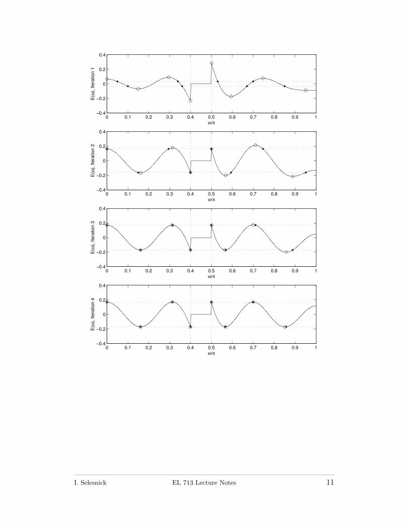
Generally, the new reference set is found by taking the set of local

minima and maxima of E(ω) that exceed the current value of δ,

and taking a subset of this set that satisfies the alternation property.

The procedure to update the set of interpolation points (the refer-

ence set) is best illustrated by an example. In the following figures,

the design of a type I FIR filter of length 13 is shown, with the

pass-band and stop-band edges at ωp = 0.4π and ωs = 0.5π, and

weights Kp = 1, Ks = 2.

The solid circular marks indicate the reference set for iteration k.

The open circular marks indicate the new reference set. They are

the local minima and maxima of the current error function, chosen

so that (1) the sign of the error alternates from point to point,

and (2) the error function at the new points is not lower than the

current value of |δ|. Note that the value of |δ| is shown by a dotted

line.


0 0.1 0.2 0.3 0.4 0.5 0.6 0.7 0.8 0.9 1−0.4

−0.2

0

0.2

0.4

E(ω

), I

tera

tio

n 1

ω/π

0 0.1 0.2 0.3 0.4 0.5 0.6 0.7 0.8 0.9 1−0.4

−0.2

0

0.2

0.4

E(ω

), Ite

ration

2

ω/π

0 0.1 0.2 0.3 0.4 0.5 0.6 0.7 0.8 0.9 1−0.4

−0.2

0

0.2

0.4

E(ω

), Ite

ratio

n 3

ω/π

0 0.1 0.2 0.3 0.4 0.5 0.6 0.7 0.8 0.9 1−0.4

−0.2

0

0.2

0.4

E(ω

), Ite

ration

4

ω/π


0 0.1 0.2 0.3 0.4 0.5 0.6 0.7 0.8 0.9 1−0.5

0

0.5

1

1.5

A(ω

), I

tera

tio

n 1

ω/π

0 0.1 0.2 0.3 0.4 0.5 0.6 0.7 0.8 0.9 1−0.5

0

0.5

1

1.5

A(ω

), Ite

ration

2

ω/π

0 0.1 0.2 0.3 0.4 0.5 0.6 0.7 0.8 0.9 1−0.5

0

0.5

1

1.5

A(ω

), Ite

ratio

n 3

ω/π

0 0.1 0.2 0.3 0.4 0.5 0.6 0.7 0.8 0.9 1−0.5

0

0.5

1

1.5

A(ω

), Ite

ration

4

ω/π

The value of |δ| and the value of the maximum value of the weighted

error ||E(ω)||∞ are given in the table for each iteration k. It can

be seen in the table that |δ| increases from iteration to iteration.

In fact, it is always the case that |δ| is monotonically increasing

(until convergence is achieved). The table also shows that for this

example, ||Ek(ω)||∞ decreases from iteration to iteration, but this


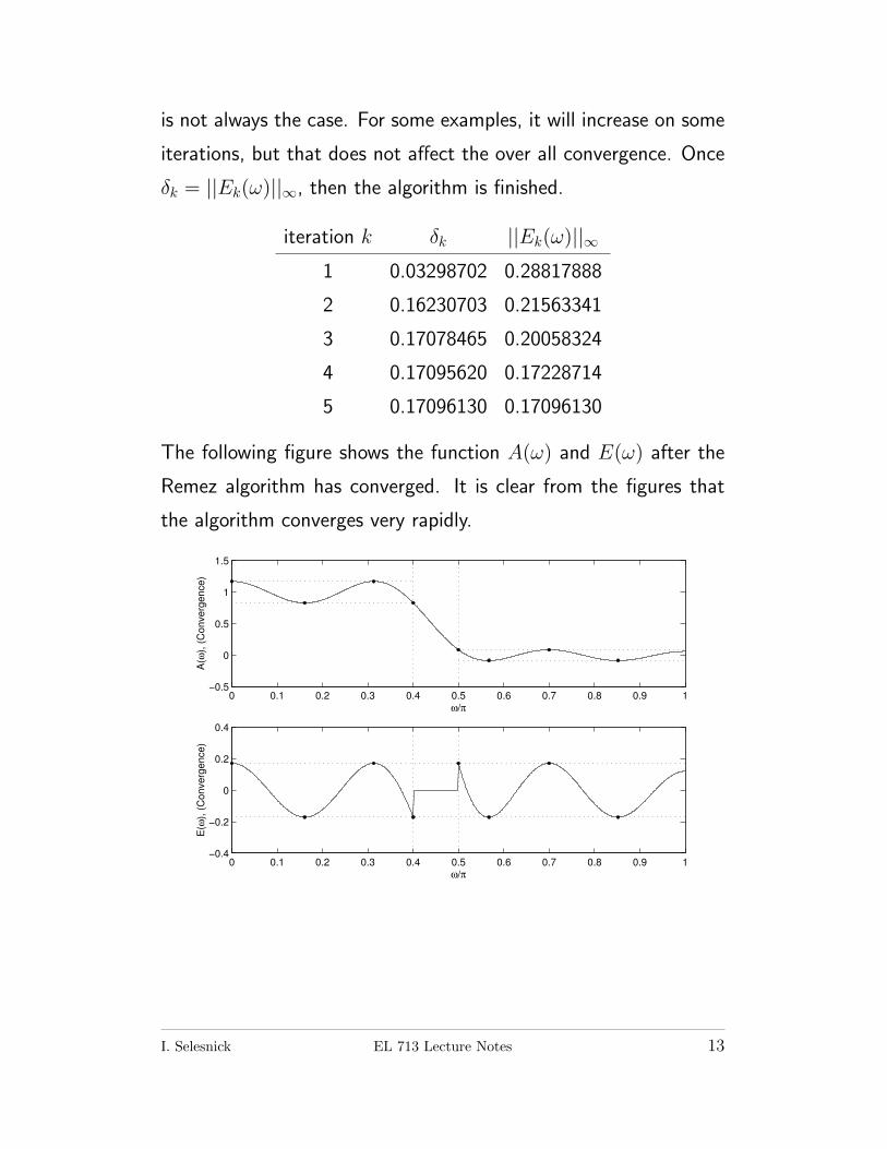
is not always the case. For some examples, it will increase on some

iterations, but that does not affect the over all convergence. Once

δk = ||Ek(ω)||∞, then the algorithm is finished.

iteration k δk ||Ek(ω)||∞1 0.03298702 0.28817888

2 0.16230703 0.21563341

3 0.17078465 0.20058324

4 0.17095620 0.17228714

5 0.17096130 0.17096130

The following figure shows the function A(ω) and E(ω) after the

Remez algorithm has converged. It is clear from the figures that

the algorithm converges very rapidly.

0 0.1 0.2 0.3 0.4 0.5 0.6 0.7 0.8 0.9 1−0.5

0

0.5

1

1.5

A(ω

), (

Converg

ence)

ω/π

0 0.1 0.2 0.3 0.4 0.5 0.6 0.7 0.8 0.9 1−0.4

−0.2

0

0.2

0.4

E(ω

), (

Converg

ence)

ω/π


IMPLEMENTING THE REMEZ ALGORITHM

To make the Remez algorithm clear, we show how it can be imple-

mented in Matlab, using the length 13 filter as an example, with

ωp = 0.4π and ωs = 0.5π and weights Kp = 1, Ks = 2.

Before the program can begin, we must define the filter specifica-

tions and set up the discretized versions of ω, W (ω) and D(ω).

The result of the comparison command yields a vector of ones and

zeros, so W and D can be built using them.

N = 13; % filter length

Kp = 1; % pass-band weight

Ks = 2; % stop-band weight

wp = 0.4*pi; % pass-band edge

ws = 0.5*pi; % stop-band edge

wo = (wp+ws)/2; % cut-off freq.

L = 1000; % grid size

w = [0:L]’*pi/L; % frequency

W = Kp*(w<=wp) + Ks*(w>=ws); % weight function

D = (w<=wo); % desired function

The first part of the program defines M , R. For this example,

M = 6, R = 8.

M = (N-1)/2;

R = M + 2; % R = size of reference set

Next, we initialize the reference set. We can do this by specifying

the indices k in the vector w. They can be chosen randomly, with

the stipulation that W (ω) is not zero at any of the points. For

example:

% initialize reference set

k = [51 101 341 361 531 671 701 851];

The actual 8 frequency values can be obtained by w(k)/pi,


>> w(k)’/pi

0.0500 0.1000 0.3400 0.3600 0.5300 0.6700 0.7000 0.8500

Iteration 1: Iteration 1 can now begin, by solving the interpolation

problem to obtain a(n) and δ.

m = 0:M;

s = (-1).^(1:R)’;

x = [cos(w(k)*m), s./W(k)] \ D(k);

a = x(1:M+1);

del = x(M+2);

The value of δ is:

>> del

0.0330

We can compute the frequency response amplitude A(ω) on the

uniformly discretized frequency ωk using the previously developed

Matlab function firamp.

h = [a(M+1:-1:2); 2*a(1); a(2:M+1)]/2;

A = firamp(h,1,L)’;

err = (A-D).*W;

We can verify that for the interpolation points, the error function

E(ω) has a constant value but alternates sign:

>> [w(k)/pi err(k)]

0.0500 0.0330

0.1000 -0.0330

0.3400 0.0330

0.3600 -0.0330

0.5300 0.0330

0.6700 -0.0330

0.7000 0.0330

0.8500 -0.0330

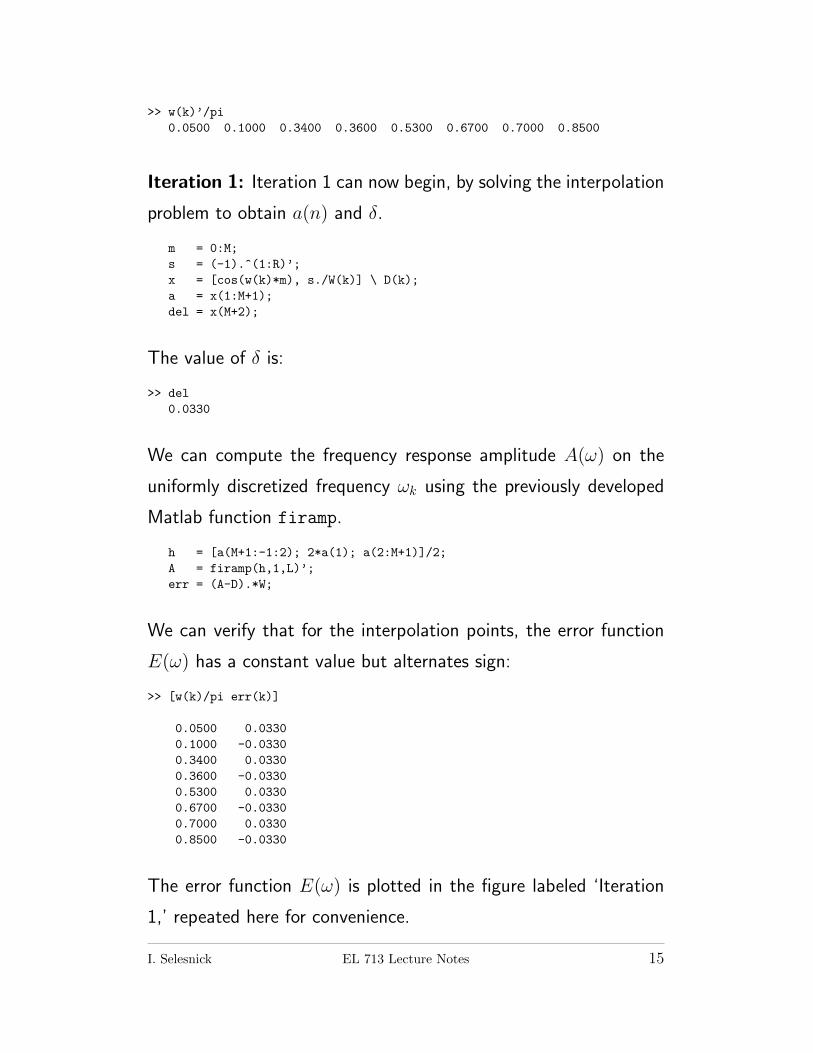
The error function E(ω) is plotted in the figure labeled ‘Iteration

1,’ repeated here for convenience.


0 0.1 0.2 0.3 0.4 0.5 0.6 0.7 0.8 0.9 1−0.4

−0.2

0

0.2

0.4

E(ω

), I

tera

tio

n 1

ω/π

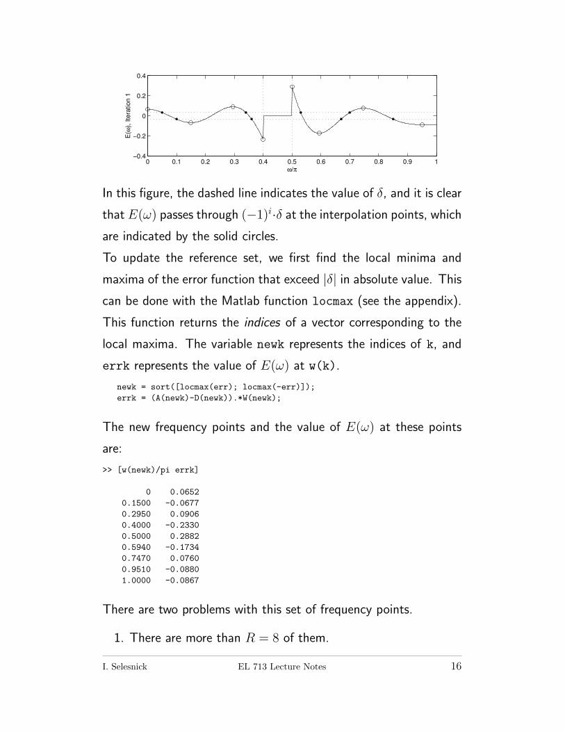
In this figure, the dashed line indicates the value of δ, and it is clear

that E(ω) passes through (−1)i·δ at the interpolation points, which

are indicated by the solid circles.

To update the reference set, we first find the local minima and

maxima of the error function that exceed |δ| in absolute value. This

can be done with the Matlab function locmax (see the appendix).

This function returns the indices of a vector corresponding to the

local maxima. The variable newk represents the indices of k, and

errk represents the value of E(ω) at w(k).

newk = sort([locmax(err); locmax(-err)]);

errk = (A(newk)-D(newk)).*W(newk);

The new frequency points and the value of E(ω) at these points

are:

>> [w(newk)/pi errk]

0 0.0652

0.1500 -0.0677

0.2950 0.0906

0.4000 -0.2330

0.5000 0.2882

0.5940 -0.1734

0.7470 0.0760

0.9510 -0.0880

1.0000 -0.0867

There are two problems with this set of frequency points.

1. There are more than R = 8 of them.


2. The function E(ω) does not alternate sign on them. (The last

two points have the same sign.)

Therefore, one of these frequencies must be dropped from this set.

This is done with a sub-program called etap which returns a set of

indices. (See the appendix.)

v = etap(errk); % ensure the alternation property

newk = newk(v);

errk = errk(v);

The new newk and errk are:


0 0.0652

0.1500 -0.0677

0.2950 0.0906

0.4000 -0.2330

0.5000 0.2882

0.5940 -0.1734

0.7470 0.0760

0.9510 -0.0880

They are indicated in the figure by open circles. Now there are the

correct number of points (R = 8), they alternate in sign, and the

are all greater than the current value of |δ| = 0.0330. So we can

replace the reference set by the new one

k = newk;

and go on to the second iteration.

Iteration 2: Iteration 2 begins by solving the interpolation problem

with the updated reference points and finding the local minima and

maxima of the resulting function E(ω). This is done with the same

commands used for iteration 1:


x = [cos(w(k)*m), s./W(k)] \ D(k);

a = x(1:M+1);

del = x(M+2);

h = [a(M+1:-1:2); 2*a(1); a(2:M+1)]/2;


err = (A-D).*W;



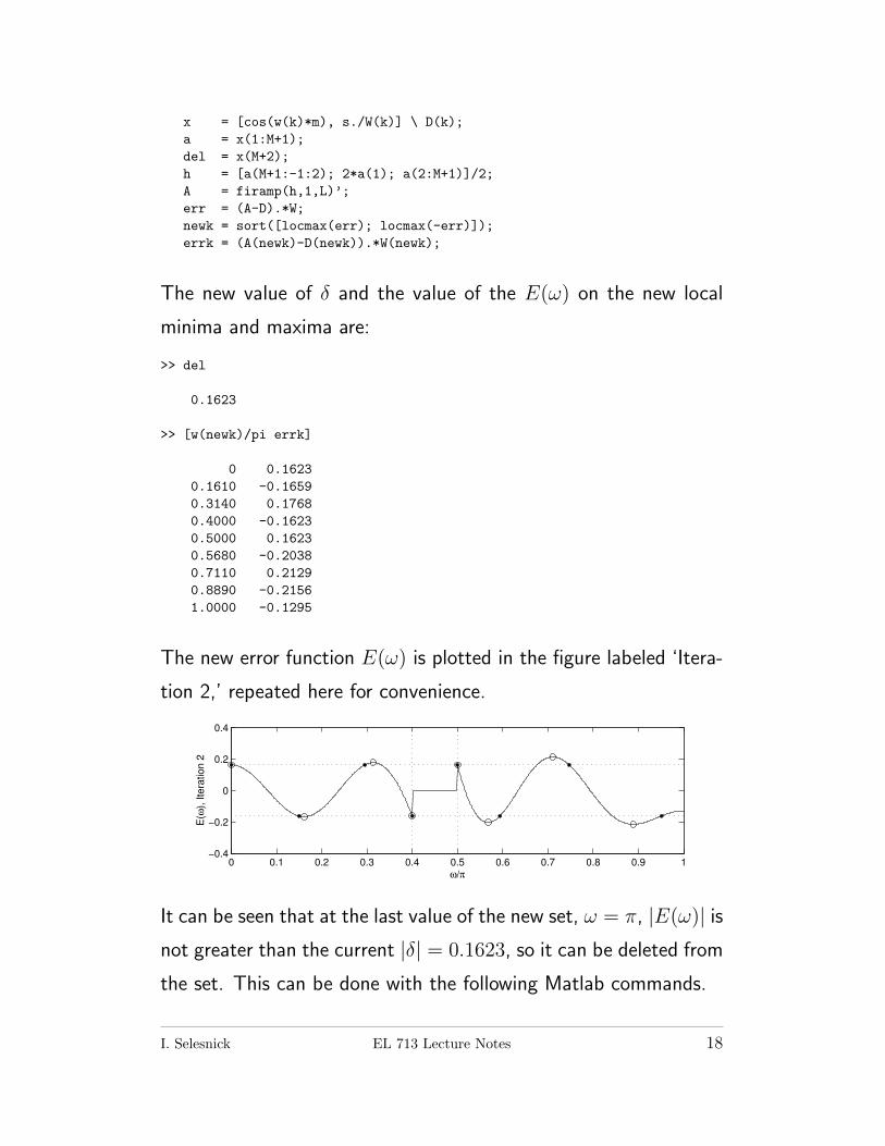
The new value of δ and the value of the E(ω) on the new local

minima and maxima are:

>> del

0.1623


0 0.1623

0.1610 -0.1659

0.3140 0.1768

0.4000 -0.1623

0.5000 0.1623

0.5680 -0.2038

0.7110 0.2129

0.8890 -0.2156

1.0000 -0.1295

The new error function E(ω) is plotted in the figure labeled ‘Itera-

tion 2,’ repeated here for convenience.

0 0.1 0.2 0.3 0.4 0.5 0.6 0.7 0.8 0.9 1−0.4

−0.2

0

0.2

0.4

E(ω

), Ite

ration

2

ω/π

It can be seen that at the last value of the new set, ω = π, |E(ω)| isnot greater than the current |δ| = 0.1623, so it can be deleted from

the set. This can be done with the following Matlab commands.


SN = 1e-8;

v = abs(errk) >= (abs(del)-SN);

newk = newk(v);

errk = errk(v);

The vector v are those indices corresponding to points where |E(ωk)|is equal to or greater than the current value of |δ|. It is necessary to

subtract a small number (SN) from |δ| to address the comparison

of two equal numbers in finite precision arithmetic. The corrected

set of points is


0 0.1623

0.1610 -0.1659

0.3140 0.1768

0.4000 -0.1623

0.5000 0.1623

0.5680 -0.2038

0.7110 0.2129

0.8890 -0.2156

They are shown as open circles in the figure. This set of points

satisfy the conditions for the update of the reference set, so we can

replace the reference set by the new one

k = newk;

and go on to the next iteration.

Putting these commands together we get a program for designing

type 1 FIR filters that minimize the Chebyshev criterion.

function [h,del] = fircheb(N,D,W)

% h = fircheb(N,D,W)

% weighted Chebyshev design of Type I FIR filters

%

% h : length-N impulse response

% N : length of filter (odd)

% D : ideal response (uniform grid)

% W : weight function (uniform grid)

% need: length(D) == length(W)


%

% % Example

% N = 31; Kp = 1; Ks = 4;

% wp = 0.26*pi; ws = 0.34*pi; wo = 0.3*pi;

% L = 1000;

% w = [0:L]*pi/L;

% W = Kp*(w<=wp) + Ks*(w>=ws);

% D = (w<=wo);

% h = fircheb(N,D,W);

% subprograms: locmax.m, etap.m

W = W(:);

D = D(:);

L = length(W)-1;

SN = 1e-8; % small number for stopping criteria, etc

M = (N-1)/2;

R = M + 2; % R = size of reference set

% initialize reference set (approx equally spaced where W>0)

f = find(W>SN);

k = f(round(linspace(1,length(f),R)));

w = [0:L]’*pi/L;

m = 0:M;

s = (-1).^(1:R)’; % signs

while 1

% --------------- Solve Interpolation Problem ---------------------

x = [cos(w(k)*m), s./W(k)] \ D(k);

a = x(1:M+1); % cosine coefficients

del = x(M+2); % delta

h = [a(M+1:-1:2); 2*a(1); a(2:M+1)]/2;


err = (A-D).*W; % weighted error

% --------------- Update Reference Set ----------------------------



% remove frequencies where the weighted error is less than delta

v = abs(errk) >= (abs(del)-SN);

newk = newk(v);

errk = errk(v);

% ensure the alternation property

v = etap(errk);

newk = newk(v);

errk = errk(v);


% if newk is too large, remove points until size is correct

while length(newk) > R

if abs(errk(1)) < abs(errk(length(newk)))

newk(1) = [];

else

newk(length(newk)) = [];

end

end

% --------------- Check Convergence -------------------------------

if (max(errk)-abs(del))/abs(del) < SN

disp(’I have converged.’)

break

end

k = newk;

end

del = abs(del);

h = [a(M+1:-1:2); 2*a(1); a(2:M+1)]/2;

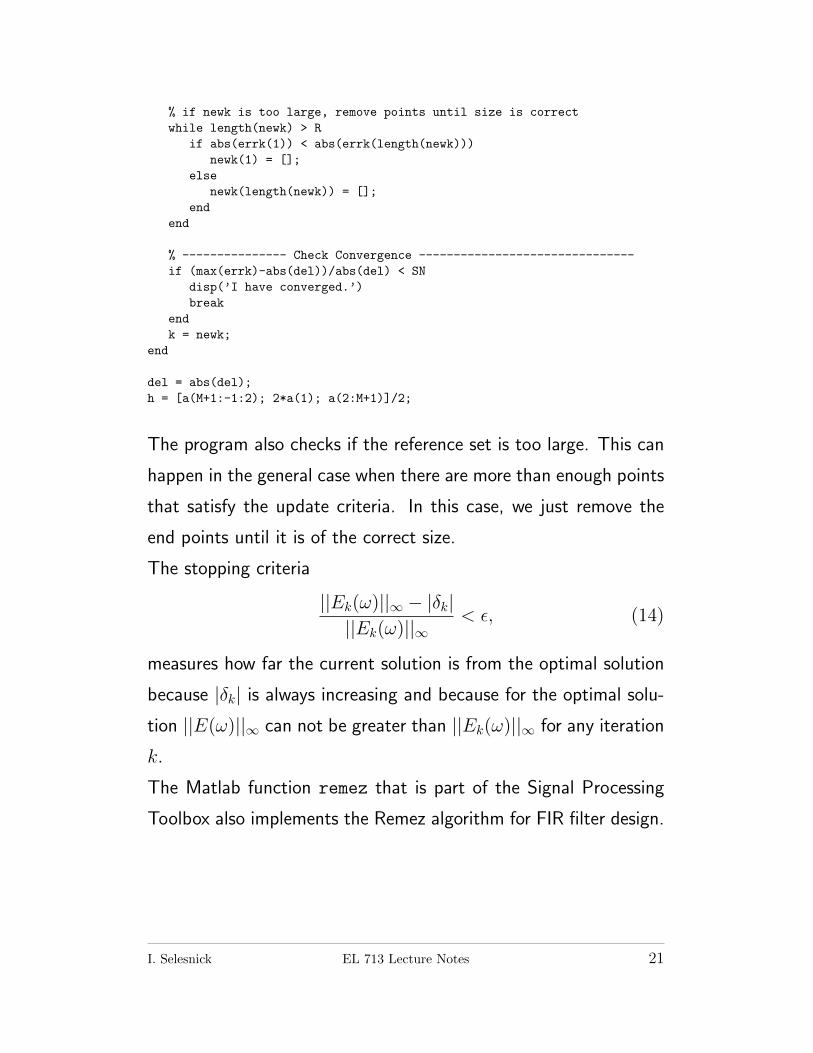
The program also checks if the reference set is too large. This can

happen in the general case when there are more than enough points

that satisfy the update criteria. In this case, we just remove the

end points until it is of the correct size.

The stopping criteria

||Ek(ω)||∞ − |δk|||Ek(ω)||∞

< ε, (14)

measures how far the current solution is from the optimal solution

because |δk| is always increasing and because for the optimal solu-

tion ||E(ω)||∞ can not be greater than ||Ek(ω)||∞ for any iteration

k.

The Matlab function remez that is part of the Signal Processing

Toolbox also implements the Remez algorithm for FIR filter design.


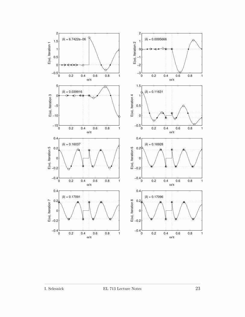
Robust Convergence of the Remez Algorithm

The Remez algorithm has very robust convergence properties. Even

if the initial interpolation points are very different from the ex-

tremal points of the optimal solution, the Remez algorithm con-

verges rapidly. In the following example, the design of the length

13 filter in the previous example is repeated, but with initial interpo-

lation points that are more different from the final extremal points.

In particular, the number of interpolation points in the pass-band

and stop-band respectively is 6 and 2 at iteration 1, but the Remez

algorithm ends up with 4 in each band which is correct for this

example.


0 0.2 0.4 0.6 0.8 1−0.5

0

0.5

1

1.5

2

E(ω

), I

tera

tion 1

ω/π

|δ| = 6.7422e−06

0 0.2 0.4 0.6 0.8 1−3

−2

−1

0

1

2

E(ω

), I

tera

tion 2

ω/π

|δ| = 0.0095666

0 0.2 0.4 0.6 0.8 1−15

−10

−5

0

5

E(ω

), Ite

ration 3

ω/π

|δ| = 0.039916

0 0.2 0.4 0.6 0.8 1−0.5

0

0.5

1

1.5

E(ω

), Ite

ration 4

ω/π

|δ| = 0.11631

0 0.2 0.4 0.6 0.8 1−0.4

−0.2

0

0.2

0.4

E(ω

), Ite

ration 5

ω/π

|δ| = 0.16037

0 0.2 0.4 0.6 0.8 1−0.4

−0.2

0

0.2

0.4

E(ω

), Ite

ration 6

ω/π

|δ| = 0.16928

0 0.2 0.4 0.6 0.8 1−0.4

−0.2

0

0.2

0.4

E(ω

), Ite

ration 7

ω/π

|δ| = 0.17091

0 0.2 0.4 0.6 0.8 1−0.4

−0.2

0

0.2

0.4

E(ω

), Ite

ration 8

ω/π

|δ| = 0.17096


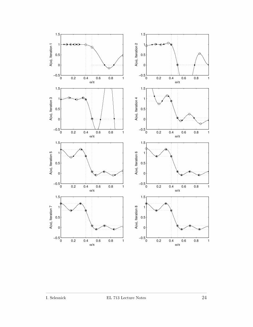
0 0.2 0.4 0.6 0.8 1−0.5

0

0.5

1

1.5

A(ω

), I

tera

tion 1

ω/π

0 0.2 0.4 0.6 0.8 1−0.5

0

0.5

1

1.5

A(ω

), I

tera

tion 2

ω/π

0 0.2 0.4 0.6 0.8 1−0.5

0

0.5

1

1.5

A(ω

), Ite

ration 3

ω/π

0 0.2 0.4 0.6 0.8 1−0.5

0

0.5

1

1.5

A(ω

), Ite

ration 4

ω/π

0 0.2 0.4 0.6 0.8 1−0.5

0

0.5

1

1.5

A(ω

), Ite

ration 5

ω/π

0 0.2 0.4 0.6 0.8 1−0.5

0

0.5

1

1.5

A(ω

), Ite

ration 6

ω/π

0 0.2 0.4 0.6 0.8 1−0.5

0

0.5

1

1.5

A(ω

), Ite

ration 7

ω/π

0 0.2 0.4 0.6 0.8 1−0.5

0

0.5

1

1.5

A(ω

), Ite

ration 8

ω/π


DESIGN RULES FOR LOW-PASS FILTERS

While the PM algorithm is applicable for the approximation of ar-

bitrary responses D(ω), the low-pass case has received particular

attention [3, 4, 10, 13]. In the design of low-pass filters via the PM

algorithm, there are five parameters of interest:

N : filter length

ωp : pass-band edge

ωs : stop-band edge

δp : maximum pass-band error

δs : maximum stop-band error

Their values are not independent — any four determines the fifth.

Formulas for predicting the required filter length for a given set

of specifications make this clear. Kaiser developed the following

approximate relation for estimating the filter length for meeting the

specifications,

N ≈−20 log10(

√δpδs)− 13

14.6∆F+ 1 (15)

where ∆F = (ωs−ωp)/(2π). Herrmann et al. [3] gave a somewhat

more accurate formula

N ≈ D∞(δp, δs)− f(δp, δs)(∆F )2

∆F+ 1 (16)

where

D∞(δp, δs) =(0.005309(log10 δp)2 + 0.07114 log10 δp − 0.4761) log10 δs

− (0.00266(log10 δp)2 + 0.5941 log10 δp + 0.4278),

(17)


f(δp, δs) = 11.01217 + 0.51244(log10 δp − log10 δs). (18)

These formulas assume that δs < δp. If otherwise, then one must

interchange δp and δs. This formula is implemented in the Matlab

function remezord in the Signal Processing Toolbox.

To use the PM algorithm for low-pass filter design, the user spec-

ifies N,ωp, ωs, δp/δs. The PM algorithm can be modified so that

the user specifies other parameters sets however [17]. For exam-

ple, with one modification, the user specifies N,ωp, δp, δs; or sim-

ilarly, N,ωs, δp, δs. With a second modification, the user specifies

N,ωp, ωp, δp; or similarly, N,ωs, ωp, δs. The necessary modifications

are simple.

Note that both (15) and (16) state that the filter length N and the

transition width ∆F are inversely proportional (for (16), as ∆F

goes to 0). This is in contrast to the corresponding relation for

maximally flat symmetric filters (covered in another section). For

equiripple filters with fixed δp and δs, ∆F diminishes like 1/N ; while

for maximally-flat filters, ∆F diminishes like 1/√N .


TRANSITION BAND ANOMALIES

Band-pass filters that minimize the Chebyshev error can be designed

with functions D(ω) and W (ω) that have the following form.

ωD(ω)

0 π

1

ωW (ω)

0 π

Ks1

Kp

Ks2

It should be noted that when a zero weighted transition band is

used (W (ω) = 0 for some interval in (0, π)), then the best Cheby-

shev solution may have undesirable behavior in those bands: large

peaks may occur. Although this does not occur in low-pass filter

design, it is well documented in band-pass filter design, in partic-

ular, when one transition band is much larger than the other. For

example, consider the design of band-pass filter with the following

specifications

−δs1 ≤ A(ω) ≤ δs1, 0 ≤ ω ≤ ωs1

1− δp ≤ A(ω) ≤ 1 + δp, ωp1 ≤ ω ≤ ωp2

−δs2 ≤ A(ω) ≤ δs2, ωs2 ≤ ω ≤ π

(19)

where

δs1 = 0.001, δp = 0.01, δs2 = 0.01, (20)


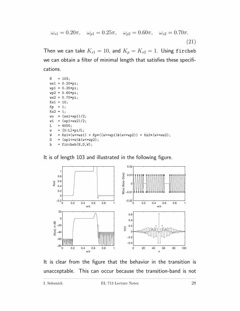
ωs1 = 0.20π, ωp1 = 0.25π, ωp2 = 0.60π, ωs2 = 0.70π.

(21)

Then we can take Ks1 = 10, and Kp = Ks2 = 1. Using fircheb

we can obtain a filter of minimal length that satisfies these specifi-

cations.

N = 103;

ws1 = 0.20*pi;

wp1 = 0.25*pi;

wp2 = 0.60*pi;

ws2 = 0.70*pi;

Ks1 = 10;

Kp = 1;

Ks2 = 1;

wo = (ws1+wp1)/2;

w1 = (wp1+ws2)/2;

L = 4000;

w = [0:L]*pi/L;

W = Ks1*(w<=ws1) + Kp*((w>=wp1)&(w<=wp2)) + Ks2*(w>=ws2);

D = (wp1<=w)&(w<=wp2);

h = fircheb(N,D,W);

It is of length 103 and illustrated in the following figure.

0 0.2 0.4 0.6 0.8 1−0.2

0

0.2

0.4

0.6

0.8

1

ω/π

A(ω

)

0 0.2 0.4 0.6 0.8 1−0.02

−0.01

0

0.01

0.02

ω/π

W(ω

) (A

(ω)−

D(ω

))

0 0.2 0.4 0.6 0.8 1−80

−60

−40

−20

0

20

ω/π

|A(ω

)|, in

dB

0 20 40 60 80 100

−0.4

−0.2

0

0.2

0.4

0.6

n

h(n

)

It is clear from the figure that the behavior in the transition is

unacceptable. This can occur because the transition-band is not


included in the criteria (the weight function W (ω) is zero there).

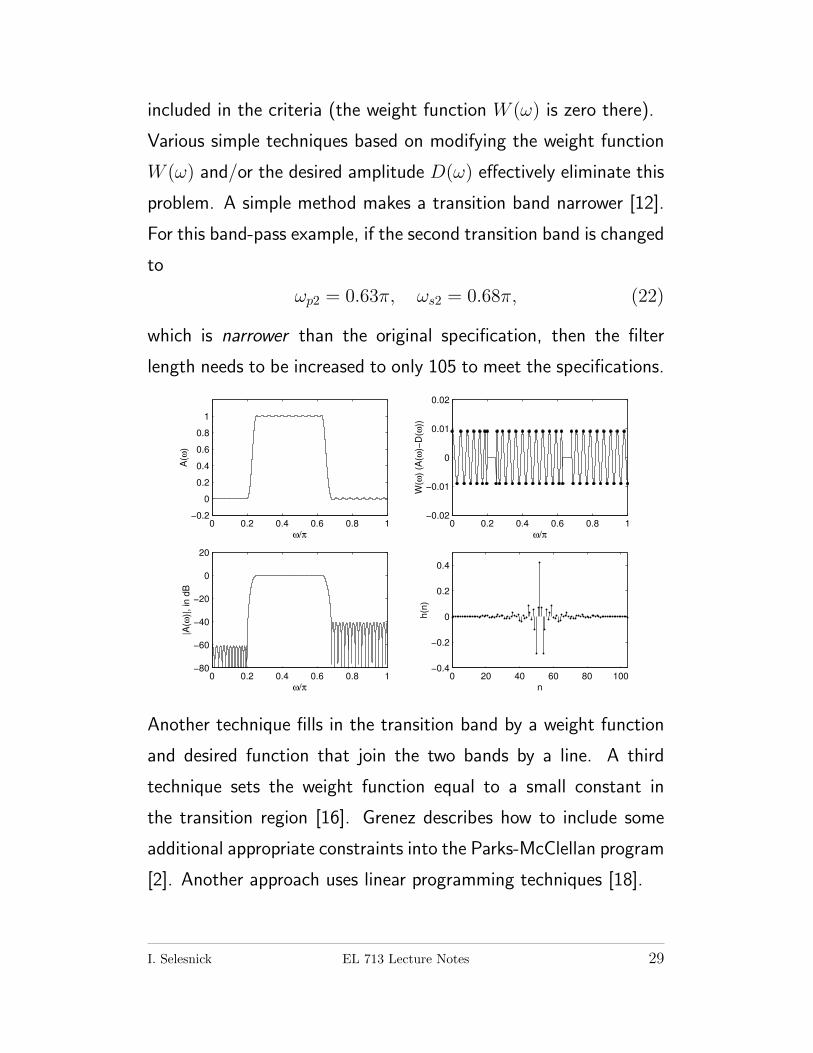
Various simple techniques based on modifying the weight function

W (ω) and/or the desired amplitude D(ω) effectively eliminate this

problem. A simple method makes a transition band narrower [12].

For this band-pass example, if the second transition band is changed

to

ωp2 = 0.63π, ωs2 = 0.68π, (22)

which is narrower than the original specification, then the filter

length needs to be increased to only 105 to meet the specifications.

0 0.2 0.4 0.6 0.8 1−0.2

0

0.2

0.4

0.6

0.8

1

ω/π

A(ω

)

0 0.2 0.4 0.6 0.8 1−0.02

−0.01

0

0.01

0.02

ω/π

W(ω

) (A

(ω)−

D(ω

))

0 0.2 0.4 0.6 0.8 1−80

−60

−40

−20

0

20

ω/π

|A(ω

)|,

in d

B

0 20 40 60 80 100−0.4

−0.2

0

0.2

0.4

n

h(n

)

Another technique fills in the transition band by a weight function

and desired function that join the two bands by a line. A third

technique sets the weight function equal to a small constant in

the transition region [16]. Grenez describes how to include some

additional appropriate constraints into the Parks-McClellan program

[2]. Another approach uses linear programming techniques [18].


CHEBYSHEV DESIGN WITH A SPECIFIED NULL

If it is desired that the filter have a null at a specified frequency, then

the Remez algorithm can still be used, but with modified functions

D(ω) and A(ω).

If the filter h(n) of length N has a null at a specified frequency

ωn,

A(ωn) = 0, (23)

then the transfer function H(z) can be factored as

H(z) = H1(z)H2(z) (24)

where h2(n) is of length N2 = N − 2 and h1(n) is of length 3 and

has the transfer function:

H1(z) = (z−1 − ejωn) (z−1 − e−jωn) (25)

= z−2 − z−1 (ejωn + e−jωn) + 1 (26)

= z−2 − 2z−1 cos(ωn) + 1 (27)

= z−1(z−1 − 2 cos(ωn) + z

)(28)

so the impulse response of is

h1 = [1, −2 cos(ωn), 1] (29)

and the frequency response is

H1(ejω) = e−jω

(ejω − 2 cos(ωn) + e−jω

)(30)

= e−jω (2 cos(ω)− 2 cos(ωn)) (31)

= e−jωA1(ω) (32)


where

A1(ω) = 2 (cos(ω)− cos(ωn)) . (33)

Note that H2(ejω) can be written as

H2(ejω) = e−jM2ω A2(ω) (34)

where M2 = (N2−1)/2. Then the amplitude response of h(n) can

be written as the product

A(ω) = A1(ω)A2(ω). (35)

The weighted error function E(ω) can be written as

E(ω) = W (ω) (A(ω)−D(ω)) (36)

E(ω) = W (ω) (A1(ω)A2(ω)−D(ω)) (37)

E(ω) = W (ω)A1(ω)

(A2(ω)− D(ω)

A1(ω)

)(38)

|E(ω)| = W2(ω) |A2(ω)−D2(ω)| (39)

where

W2(ω) = |W (ω)A1(ω)| (40)

D2(ω) =D(ω)

A1(ω). (41)

Then the sought filter h(n) of length N can be found by first finding

the filter of length N2 = N −2 that minimizes the Chebyshev error

with weight function W2(ω) and desired amplitude response D2(ω),

and by then convolving it with h1(n)

h(n) = h1(n) ∗ h2(n). (42)

This procedure is implemented in the following Matlab code, for

the design of a length 31 type I FIR filter with Kp = 1, Ks = 4

and ωp = 0.26π, ωs = 0.34π.


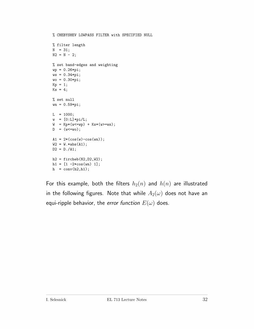
% CHEBYSHEV LOWPASS FILTER with SPECIFIED NULL

% filter length

N = 31;

N2 = N - 2;

% set band-edges and weighting

wp = 0.26*pi;

ws = 0.34*pi;

wo = 0.30*pi;

Kp = 1;

Ks = 4;

% set null

wn = 0.59*pi;

L = 1000;

w = [0:L]*pi/L;

W = Kp*(w<=wp) + Ks*(w>=ws);

D = (w<=wo);

A1 = 2*(cos(w)-cos(wn));

W2 = W.*abs(A1);

D2 = D./A1;

h2 = fircheb(N2,D2,W2);

h1 = [1 -2*cos(wn) 1];

h = conv(h2,h1);

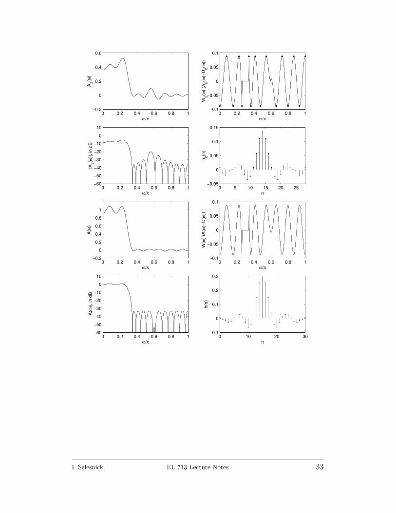
For this example, both the filters h2(n) and h(n) are illustrated

in the following figures. Note that while A2(ω) does not have an

equi-ripple behavior, the error function E(ω) does.


0 0.2 0.4 0.6 0.8 1−0.2

0

0.2

0.4

0.6

ω/π

A2(ω

)

0 0.2 0.4 0.6 0.8 1−0.1

−0.05

0

0.05

0.1

ω/π

W2(ω

) (A

2(ω

)−D

2(ω

))

0 0.2 0.4 0.6 0.8 1−60

−50

−40

−30

−20

−10

0

10

ω/π

|A2(ω

)|, in

dB

0 5 10 15 20 25−0.05

0

0.05

0.1

0.15

n

h2(n

)

0 0.2 0.4 0.6 0.8 1−0.2

0

0.2

0.4

0.6

0.8

1

ω/π

A(ω

)

0 0.2 0.4 0.6 0.8 1−0.1

−0.05

0

0.05

0.1

ω/π

W(ω

) (A

(ω)−

D(ω

))

0 0.2 0.4 0.6 0.8 1−60

−50

−40

−30

−20

−10

0

10

ω/π

|A(ω

)|, in

dB

0 10 20 30−0.1

0

0.1

0.2

0.3

n

h(n

)


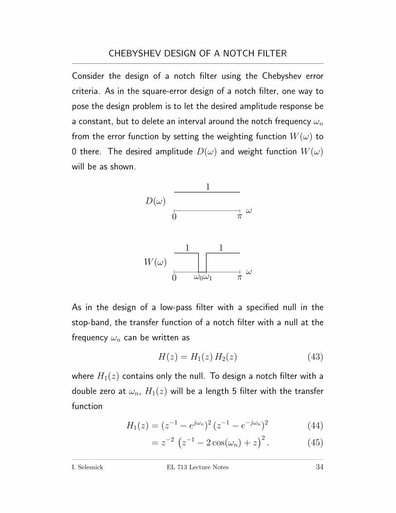
CHEBYSHEV DESIGN OF A NOTCH FILTER

Consider the design of a notch filter using the Chebyshev error

criteria. As in the square-error design of a notch filter, one way to

pose the design problem is to let the desired amplitude response be

a constant, but to delete an interval around the notch frequency ωn

from the error function by setting the weighting function W (ω) to

0 there. The desired amplitude D(ω) and weight function W (ω)

will be as shown.

ωD(ω)

0 π

1

ωW (ω)

0 ω0ω1 π

1 1

As in the design of a low-pass filter with a specified null in the

stop-band, the transfer function of a notch filter with a null at the

frequency ωn can be written as

H(z) = H1(z)H2(z) (43)

where H1(z) contains only the null. To design a notch filter with a

double zero at ωn, H1(z) will be a length 5 filter with the transfer

function

H1(z) = (z−1 − ejωn)2 (z−1 − e−jωn)2 (44)

= z−2(z−1 − 2 cos(ωn) + z

)2. (45)


Then

H1(ejω) = e−2jωA1(ω) (46)

where

A1(ω) = 4 (cos(ω)− cos(ωn))2 . (47)

H2(z) will then be of length N2 = N − 4 and can be written as

H2(z) = e−jM2ω A2(ω) (48)

where M2 = (N2 − 1)/2. The amplitude response of h(n) can be

written as the product

A(ω) = A1(ω)A2(ω). (49)

Then the weighted error function |E(ω)| can be written as

|E(ω)| = W2(ω) |A2(ω)−D2(ω)| (50)

where

W2(ω) = |W (ω)A1(ω)|, D2(ω) =D(ω)

A1(ω). (51)

As in the previous example, we first find the filter h2(n) of length

N2 = N − 4 that minimizes the Chebyshev error with weight func-

tion W2(ω) and desired amplitude response D2(ω), and then con-

volve it with h1(n).

Design example. The following Matlab code designs a length 51

Type 1 FIR notch filter according to the Chebyshev criterion with

notch frequency ωn = 0.6π, and ω0 = 0.55π, ω1 = 0.65π.

% CHEBYSHEV NOTCH FILTER

% filter length


N = 51;

N2 = N - 4;

% set band-edges

w0 = 0.55*pi;

w1 = 0.65*pi;

% set notch frequency

wn = 0.60*pi;

L = 1000;

w = [0:L]*pi/L;

W = (w<=w0) + (w>=w1);

D = ones(size(w));

A1 = 4*(cos(w)-cos(wn)).^2;

W2 = W.*abs(A1);

D2 = D./A1;

h1 = conv([1 -2*cos(wn) 1],[1 -2*cos(wn) 1]);

h2 = fircheb(N2,D2,W2);

h = conv(h2,h1);

The filter h(n) is illustrated in the following figure.


0 0.2 0.4 0.6 0.8 10

5

10

15

20

25

ω/π

A2(ω

)

0 0.2 0.4 0.6 0.8 1−0.06

−0.04

−0.02

0

0.02

0.04

0.06

ω/π

W2(ω

) (A

2(ω

)−D

2(ω

))

0 10 20 30 40−3

−2

−1

0

1

2

3

4

n

h2(n

)

−1 0 1

−1

−0.5

0

0.5

1

Ze

ros o

f H

2(z

)

0 0.2 0.4 0.6 0.8 1−0.2

0

0.2

0.4

0.6

0.8

1

ω/π

A(ω

)

−1 0 1

−1

−0.5

0

0.5

1

Zero

s o

f H

(z)

2

2

0 0.2 0.4 0.6 0.8 1−60

−50

−40

−30

−20

−10

0

10

ω/π

|A(ω

)|, in

dB

0 10 20 30 40 50−0.2

0

0.2

0.4

0.6

0.8

1

n

h(n

)


B ETAP.M

REMEZ ALGORITHM: ADVANTAGES AND DISADVANTAGES

• Produces linear-phase FIR filters that minimize the weighted

Chebyshev error.

• Provides explicit control of band edges and relative ripple sizes.

• Efficient algorithm, always converges.

• Allows the use of a frequency dependent weighting function.

• Suitable for arbitrary D(ω) and W (ω).

• Does not allow arbitrary linear constraints.

A locmax.m

function maxind = locmax(x)

% function maxind = locmax(x)

% finds indices of local maxima of data x

x = x(:);

n = length(x);

maxind = find(x > [x(1)-1;x(1:n-1)] & x > [x(2:n);x(n)-1]);

B etap.m

function v = etap(E)

%

% v = etap(E);

% Ensuring The Alternation Property

% E : error vector

% v : index of original E

if size(E,1) > 1

a = 1;

else

a = 0;


REFERENCES REFERENCES

end

j = 1;

xe = E(1);

xv = 1;

for k = 2:length(E)

if sign(E(k)) == sign(xe)

if abs(E(k)) > abs(xe)

xe = E(k);

xv = k;

end

else

v(j) = xv;

j = j + 1;

xe = E(k);

xv = k;

end

end

v(j) = xv;

if a == 1

v = v(:);

end

References

[1] IEEE DSP Committee, editor. Selected Papers In Digital Signal Processing,II. IEEE Press,

1976.

[2] F. Grenez. Design of linear or minimum-phase FIR filters by constrained Chebyshev

approximation. Signal Processing, 5:325–332, May 1983.

[3] O. Herrmann, L. R. Rabiner, and D. S. K. Chan. Practical design rules for optimum finite

impulse response lowpass digital filters. The Bell System Technical Journal, 52:769–799,

1973.

[4] J. F. Kaiser. Nonrecursive digital filter design using the Io-sinh window function. In

Proc. IEEE Int. Symp. Circuits and Systems (ISCAS), pages 20–23, April 1974. Also in

[1].

[5] J. H. McClellan and T. W. Parks. A unified approach to the design of optimum FIR

linear-phase digital filters. IEEE Trans. on Circuit Theory, 20:697–701, November 1973.

[6] J. H. McClellan, T. W. Parks, and L. R. Rabiner. A computer program for designing

optimum FIR linear phase digital filters. IEEE Trans. Audio Electroacoust., 21:506–526,

December 1973. Also in [1].

[7] A. V. Oppenheim and R. W. Schafer. Discrete-Time Signal Processing. Prentice Hall,

1989.


REFERENCES REFERENCES

[8] T. W. Parks and C. S. Burrus. Digital Filter Design. John Wiley and Sons, 1987.

[9] T. W. Parks and J. H. McClellan. Chebyshev approximation for nonrecursive digital filters

with linear phase. IEEE Trans. on Circuit Theory, 19:189–94, March 1972.

[10] T. W. Parks and J. H. McClellan. On the transition region width of finite impulse-response

digital filters. IEEE Trans. Audio Electroacoust., 21:1–4, February 1973.

[11] M. J. D. Powell. Approximation Theory and Methods. Cambridge University Press, 1981.

[12] L. Rabiner, J. Kaiser, and R. Schafer. Some considerations in the design of multiband

finite-impulse-response digital filters. IEEE Trans. on Acoust., Speech, Signal Proc.,

22(6):462–472, December 1974.

[13] L. R. Rabiner. Approximate design relationships for lowpass FIR digital filters. IEEE

Trans. Audio Electroacoust., 21:456–460, October 1973. Also in [1].

[14] L. R. Rabiner and B. Gold. Theory and Application of Digital Signal Processing. Prentice

Hall, Englewood Cliffs, NJ, 1975.

[15] L. R. Rabiner, J. H. McClellan, and T. W. Parks. FIR digital filter design techniques

using weighted Chebyshev approximation. Proc. IEEE, 63(4):595–610, April 1975. Also

in [1].

[16] T. Saramaki. Finite impulse resonse filter design. In S. K. Mitra and J. F. Kaiser, editors,

Handbook For Digital Signal Processing, chapter 4, pages 155–277. John Wiley and Sons,

1993.

[17] I. W. Selesnick and C. S. Burrus. Exchange algorithms that complement the Parks-

McClellan algorithm for linear phase FIR filter design. IEEE Trans. on Circuits and

Systems II, 44(2):137–142, February 1997.

[18] K. Steiglitz, T. W. Parks, and J. F. Kaiser. METEOR: A constraint-based FIR filter

design program. IEEE Trans. Signal Process., 40(8):1901–1909, August 1992.


Documents

THE REMEZ ALGORITHM - NYU Tandon School of …eeweb.poly.edu/iselesni/EL713/remez/remez.pdf · the value is taken as a variable in this interpolation problem, so ... is not always