Embed Size (px)
Citation preview

Progress In Electromagnetics Research B, Vol. 16, 21–56, 2009
THE RELATIVISTIC HERMITE POLYNOMIALS ANDTHE WAVE EQUATION
A. Torre
ENEA-FIM-FISMAT Tecnologie Fisiche e Nuovi Materialivia E. Fermi 45, Frascati, Rome 00044, Italy
Abstract—Solutions of the homogeneous 2D scalar wave equation ofa type reminiscent of the “splash pulse” waveform are investigated insome detail. In particular, it is shown that the “higher-order” solutionsrelative to a given “fundamental” one, from which they are obtainedthrough a definite “generation scheme”, come to involve the relativisticHermite polynomials. This parallels the results of a previous work,where solutions of the 3D wave equation involving the relativisticLaguerre polynomials have been suggested. Then, exploiting a wellknown rule, the obtained wave functions are used to construct furthersolutions of the 3D wave equation. The link of the resulting wavefunctions with those analyzed in the previous work is clarified, thepertinent generation scheme being indeed inferred. Finally, solutionsof the Klein-Gordon equation which relate to such Lorentzian-likesolutions of the scalar wave equation are deduced.
1. INTRODUCTION
The literature concerned with the homogeneous 3D scalar waveequation, [∇2 − c−2∂2
t
]u (x, y, z, t) = 0, (1)
is rich of transformations which allow us to pass from one solution(or, wave function) to another [1–7]. Needless to say, here u (x, y, z, t)represents the scalar-valued wave field and c is the (constant) speedof propagation; also, (x, y, z) denote Cartesian coordinates, with inparticular z being assumed along the direction of propagation, and, ofcourse, ∇2 = ∂2
x + ∂2y + ∂2
z .In this connection, further hints have been recently suggested in [8]
and [9], on the basis of the method of incomplete separation of variables
Corresponding author: A. Torre ([email protected]).

22 Torre
and the application of the Bateman conformal transformation. Suchapproaches have then been framed in [10] within the context of thebidirectional spectral representation [11], which is shown to allow,when examined in conjuction with Bateman’s transformations, asystematic derivation of extended families of focus wave mode-typelocalized solutions of (1).
In particular, as is well known, one can pass from solutions of the2D wave equation
[∂2
q + ∂2z − c−2∂2
t
]φ (q, z, t) = 0, (2)
where q denotes any one of the two Cartesian coordinate x, y, tosolutions of the 3D wave Equation (1) according to the rule [1–7, 12]
u(x, y, z, t) = (x± iy)−12 φ(r, z, t), r =
√x2 + y2. (3)
In addition, due to the symmetry of both (1) and (2), it ispossible to generate further solutions from a known one by circularpermutations of both the space and the time coordinates, i.e., throughq ↔ z ↔ ±ict for (2) and x ↔ y ↔ z ↔ ±ict for (1). Accordingly, (3)is paralleled by another non trivial rule, obtained by transforming thetime coordinate into a space coordinate to yield
u(x, y, z, t) = (x± ct)−12 φ
(√x2 − c2t2, z,− i
cy
). (4)
Here, we are concerned with the transformation (3), which willbe applied to what can be regarded as the 2D versions of the splashpulses [13–16], that is, to 2D wave functions of the type
φ(q, z, t) =1√
τ − iz0
(σ + ia +
q2
τ − iz0
)−N
(5)
where τ and σ signify the characteristic variables τ = z − ct andσ = z + ct, N is here taken as a real positive parameter, and similarlyz0 and a are positive parameters with dimensions of length.
A renewed interest in the splash pulses
sδ(x, y, z, t) =1
τ − iz0
1(σ + ia + r2
τ−iz0
)δ, (6)
have been stimulated by the recent analysis presented in [16], where theauthors investigated the behavior of the so-called double-exponential(DEX) pulses, obtained as a suitable superposition of progressive

Progress In Electromagnetics Research B, Vol. 16, 2009 23
and regressive splash pulses (6), corresponding to in general differentvalues of the parameter a. Specifically, a detailed analysis of thebehavior of the splash and DEX pulses for values of δ within the range−0.9 ≤ δ ≤ 0.9 is presented in the quoted reference.
Also, in [17] and [18] the expression for s1(x, y, z, t) =1
(σ+ia)(τ−iz0)+r2 has been taken as a Hertz potential, respectivelyoriented parallel and orthogonal to the z-direction, from whichthe components of the corresponding vector electromagnetic fieldshave then been derived. An extensive study of the field solutions,resulting respectively in toroidal, focused doughnut wave packets andoblate wave packets, have been performed in the quoted referencesspecifically in the paraxial regime z0 ¿ a. In particular, in [18] theparaxial solutions there analyzed have been demonstrated to be thenatural spatiotemporal modes of an open electromagnetic cavity andaccordingly their physical realization has been suggested by excitationof a curved mirror resonator or by propagation along the equivalentlens waveguide.
The splash pulses for δ > 12 have been reconsidered in [19],
where the relevant higher-order pulses (there referred to as Laguerre-Lorentzian solutions of (1)), obtained through a definite generationscheme demanding for integer powers of the transverse Laplacian∇2
⊥ =∂2
x + ∂2y acting on the Lorentz-like complex function (6)†, have been
related to the relativistic Laguerre polynomials (RLP). In the samereference, the expressions of the electromagnetic field components,corresponding to the Laguerre-Lorentzian wave functions, have beenderived in particular for the TE modes, and so for a z-directed Hertzvector potential.
Paralleling the analysis developed in [19], we will show here thathigher-order solutions of the 2D wave Equation (2), obtained from thefundamental one (5) acting on it by powers of the derivative operator∂q, relate to the relativistic Hermite polynomials (RHP), which so cometo modulate the Lorentzian-like factor in the same way as the ordinaryHermite polynomials (HP) modulate the Gaussian-like factor in the 2DHermite-Gaussian pulses [20–24]. Indeed, in the solutions discussedin [19], the RLPs enter as modulating factors of suitable Lorentz-like functions in the same way as the ordinary Laguerre polynomials(LP) modulate appropriate Gaussian-like functions in the Laguerre-Gaussian pulses [20–24].† Although it is quite an improper terminology, by Lorentz-like (in general, complex)
functions we mean here functions of the type (1 + ξ2
A)−B , where ξ denotes the coordinate
of concern, A is a complex constant (i.e., independent on ξ) and B > 0. Clearly, whenreferred to a wave function, as in the present context, it will not in general yield a similarLorentz-like behavior (with respect to ξ) for the corresponding wave amplitude.

24 Torre
Then, applying the transformation (3), we will pass from theobtained solutions of the 2D wave equation to wave functions forthe 3D wave equation, which so will have the RHPs as their centralpart. Interestingly we will be successful on deducing among others,a generation scheme for the resulting 3D wave functions, that resortsto the same fundamental form of the solutions considered in [19], butdemands for half-integer powers of the same operators involved in thegeneration scheme pertaining to those solutions. This unequivocallyestablishes a link of the wave functions discussed here with thosesuggested in [19]. It is from this link that, in our opinion, the analysisdeveloped here stems its interest, as it allows us to encompass allthe wave functions of the splash pulse-type (for positive exponents)discussed here and in the previous paper [19] in a single scheme,which basically resorts to the same symmetry operators of the 3Dwave equation. It is in fact evident that what we have referred toas “generation scheme” arises from definite symmetries of the waveequation [5], and hence might comprise and possibly extend alreadyknown transformations.
We will not dwell here on the practical feasibility of the solutionsof concern in the present context, addressing the issue to future work.We note in fact through Bateman’s words ([4], P. 25) that the theory ofwave-functions forms a natural extension of the theory of functions ofcomplex variable and may consequently lead to results of great value forthe general theory of functions. Of course, the possibility of applicationto physical problems would surely increase the interest in the analysishere presented and would motivate further investigations.
Finally, possible solutions of the Klein-Gordon equation, whichstrictly relate to the Lorentzian-like wave functions, will be deducedand properly commented on in relation with pertinent results, alreadyexisting in the literature.
Let us recall now that the RHPs have been introduced less thantwo decades ago within the context of the dynamics of the quantumrelativistic 1D harmonic oscillator [25]; also, they have recently beenre-considered within the context of the paraxial wave propagationin [26], where their relation with the Lorentz beams has been evidenced.Likewise, the RLPs stand out as the relativistic version of the ordinaryLPs, their relation to the latter paralleling that of the RHPs to theordinary HPs as far as the “relativistic” parameter N is concerned [27].
Notably, both the RHPs and the RLPs are not independentpolynomials, being indeed proved to relate to the Jacobi polynomialsof suitable parameters and arguments [27–29]; specifically, the RHPsrelate to the Gegenbauer polynomials. However, since their formalexpressions allow for a direct analogy with the Hermite-Gaussian and

Progress In Electromagnetics Research B, Vol. 16, 2009 25
Laguerre-Gaussian solutions to the wave equations, we prefer to usesuch formal expressions and to refer to them in accord with the originalterminology, which has also the advantage of evoking the “relativistic”context where those expressions naturally frame.
It is worth noting that the presence of the RHPs, which asrecalled relate to the Gegenbauer polynomials, arising in connectionwith the 2D wave equation is in a sense not surprising indeed, sincethe symmetry properties of such an equation naturally relate it to theGegenbauer polynomials [5].
The plan of the paper is as follows. In Section 2, the basicproperties of the RHPs are listed. In Section 3, we relate the RHPsto the solutions of the 2D wave Equation (2). Consequences of thetransformation (3) are then investigated in Section 4, where generationschemes for the introduced Hermite-Lorentzian solutions of the 3Dwave Equation (1) are deduced; in particular, we clarify in Section 5the link of the obtained wave functions with the Laguerre-Lorentziansolutions, considered in [19]. Solutions of the Klein-Gordon equation,which relate to those of the scalar wave equation discussed in theprevious sections, are finally deduced in Section 6. Concluding notesare given in Section 7.
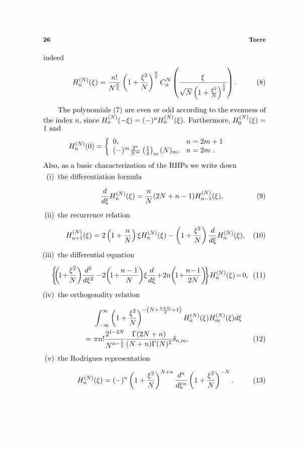
2. THE RELATIVISTIC HERMITE POLYNOMIALS:BASIC PROPERTIES
The RHPs H(N)n (ξ) have been originally introduced in the form [25]
H(N)n (ξ) =
n!2n
Γ(N + 1
2
)
Nn2
Γ(2N + n)Γ(2N)
[n2 ]∑
j=0
(−)j
j!(n−2j)!1
Γ(N+j+ 1
2
)(
2ξ√N
)n−2j
, −∞<ξ<+∞ (7)
for positive real value of the dimensionless parameter N , as thepolynomial component of the quantum relativistic harmonic oscillatorwave function. The parameter N , defined by the ratio of the oscillatorenergy mc2 to the its quantum of energy ~ω0: N = mc2
~ω0, signals the
“relativistic” character of the polynomials (7), which in fact in theasymptotic (non-relativistic) limit, c →∞ (i.e., N →∞) turn into theordinary Hermite polynomials Hn(ξ) (HP).
As mentioned earlier, the RHPs relate to the GPs CNn , being
26 Torre
indeed
H(N)n (ξ) =
n!N
n2
(1 +
ξ2
N
)n2
CNn
ξ√
N(1 + ξ2
N
) 12
. (8)
The polynomials (7) are even or odd according to the evenness ofthe index n, since H
(N)n (−ξ) = (−)nH
(N)n (ξ). Furthermore, H
(N)0 (ξ) =
1 and
H(N)n (0) =
0, n = 2m + 1(−)m 2n
Nm
(12
)m
(N)m, n = 2m .
Also, as a basic characterization of the RHPs we write down
(i) the differentiation formula
d
dξH(N)
n (ξ) =n
N(2N + n− 1)H(N)
n−1(ξ), (9)
(ii) the recurrence relation
H(N)n+1(ξ) = 2
(1 +
n
N
)ξH(N)
n (ξ)−(
1 +ξ2
N
)d
dξH(N)
n (ξ), (10)
(iii) the differential equation(
1+ξ2
N
)d2
dξ2−2
(1+
n− 1N
)ξ
d
dξ+2n
(1+
n−12N
)H(N)
n (ξ)=0, (11)
(iv) the orthogonality relation
∫ ∞
−∞
(1 +
ξ2
N
)−(N+n+m2
+1)H(N)
n (ξ)H(N)m (ξ)dξ
= πn!21−2N
Nn− 12
Γ(2N + n)(N + n)Γ(N)2
δn,m, (12)
(v) the Rodrigues representation
H(N)n (ξ) = (−)n
(1 +
ξ2
N
)N+ndn
dξn
(1 +
ξ2
N
)−N
. (13)

Progress In Electromagnetics Research B, Vol. 16, 2009 27
Then, we resort to the Hermite-Lorentzian functions (HLF)introduced in [26] as
Φ(N)n (ξ) = H(N)
n (ξ)(
1 +ξ2
N
)−(N+n)
, (14)
which, as there noted, due to the limit relation (1+ ξ2
N )−N −−−−→N→∞
e−ξ2,
can be considered as the “relativistic” limit of the elegant Hermite-Gaussian functions (EHGF) Φ(∞)
n (ξ) = Hn(ξ)e−ξ2.
It is worth noting that in [26] the parameter N has been limitedto integer values only, in order to properly refer to the factor (1 +ξ2
N )−(N+n) entering (14) as a Lorentzian (N + n = 1) or a multi-Lorentzian (N + n > 1) function as well as to work out explicitanalytical representations of the propagated beams. Here, we relaxsuch a constraint on N , letting it be an arbitrary positive realnumber, whilst retaining in a rather improper use, as already notedin the footnote on P. 3, the terminology of Lorentz-like function whenreferring to the aforementioned factor.
Figure 1 shows the plots of the HLFs for some values of n and N .To help insight into the behavior of such functions the correspondingEHGFs for each n value — the correspondence being intended in thesense of the above mentioned limit relation — are also plotted in thefigure. Actually, the graphs reproduce the normalized functions [26]
ϕ(N)n (ξ) = N (N)
n H(N)n (ξ)
(1 +
ξ2
N
)−(N+n)
, (15)
with N (N)n = 2NΓ(N)[ Nn− 1
2 Γ(N+n+ 12)
2√
πΓ(N+n)Γ(2N+n− 12)Γ(n+ 1
2)]12 , the corresponding
normalized EHGFs being ϕ(∞)n (ξ) = 1√
2n− 12 Γ(n+ 1
2)Hn(ξ)e−ξ2
.
As to the normalization factor N (N)n entering (15), we see that it
can easily be evaluated by resorting to the Parseval theorem and tothe possibility of representing the Φ(N)
n ’s as [26]
Φ(N)n (ξ) = F−1(−iκ)nF
(1 +
ξ2
N
)−N
as a consequence of the Rodrigues Formula (13); here, F signifiesFourier transform. We note that
F(
1 +ξ2
N
)−N
=√
π
2N− 32
NN− 12
Γ(N)|κ|N−1W0, N− 1
2
(2√
N |κ|)
, (16)

28 Torre
ϕ (ξ)(N)
0ϕ (ξ)(N)
1
ξ ξ
ϕ (ξ)(N)
2ϕ (ξ)(N)
3
ξ ξ
Figure 1. ξ-profiles of the HLFs ϕ(N)n ’s for n = 0, 1, 2, 3 and N = 1
(solid line), N = 5 (dash-dotted line), N = 15 (dashed line). Theprofiles of the corresponding EHGFs ϕ
(∞)n for each value of n are also
plotted, marked by the ♦’s.
where Wν, µ denotes Whittaker’s second function [30].Accordingly, the integral representation of Φ(N)
n (ξ) follows in theform
Φ(N)n (ξ)
=(−i)n
2N−2
NN− 12
Γ(N)
∫ ∞
0
cos(κξ) n eveni sin(κξ) n odd
κN+n−1W0, N− 1
2
(2√
Nκ)dκ.(17)
In this connection, we recall that W0, µ(z) =√
zπKµ( z
2), Kµ being themodified Bessel function of second kind; such a relation may help thecomparison of (17) with the expression of the integral representation of

Progress In Electromagnetics Research B, Vol. 16, 2009 29
the Laguerre-Lorentzian functions discussed in [19] (see Equation (29)there).
Also, the differential equation for the Φ(N)n ’s is easily obtained as
(1+
ξ2
N
)d2
dξ2+(n+1)
(2N+n
N
)ξ
d
dξ+2
(N+n+1
N
)Φ(N)
n (ξ)=0. (18)
Finally, for future use we report the relation between the RHPsand the RLPs, i.e.,
H(N)2m (ξ) = (−)mm!22m (N)m
NmL
(− 12,N)
m (ξ2),
H(N)2m+1(ξ) = (−)mm!22m+1 (N)m+1
Nm+1ξL
( 12,N)
m (ξ2),(19)
which is evidently reminiscent of that holding between the ordinarypolynomials, recovered indeed in the limit N → ∞ [27]. The RLPsL
(α,N)n (x) are defined by [27]
L(α, N)n (x)=Γ
(N+n+
12
) n∑
j=0
(−)j(n+αn−j
) 1j!Γ
(N+n−j+ 1
2
)(x
N
)j, (20)
which in the limit N → ∞ turns into the expression for the ordinaryLaguerre polynomials L
(α)n (x) [30]. We see that L
(α, N)n (0) = 1 and
L(α, N)0 (x) = 1; furthermore, the RLPs relate to the Jacobi polynomials
P(β,α)n , being indeed [27, 29]
L(α, N)n (x) = (−)n
(1 +
x
N
)nP
(N− 12,α)
n
(x−N
x + N
). (21)
Also, in order to facilitate subsequent checks we note that
L(−k, N)n (x) = (−)k (n− k)!
n!
( x
N
)k Γ(N + n + 1
2
)
Γ(N + n− k + 1
2
)L(k, N)n−k (x), (22)
with k integer such that 0 ≤ k ≤ n.
3. THE RELATIVISTIC HERMITE POLYNOMIALS ANDTHE 2D WAVE EQUATION
It is easy to verify that Equation (2) is solved by the function
φ0, N (x, z, t) =1√
τ − iz0
(σ + ia +
x2
τ − iz0
)−N
(23)

30 Torre
where the various parameters are chosen so that N > 0, z0 > 0, anda > 0, the latter being aimed at avoiding singularity at x = 0 andsimilarly at (z = 0, t = 0).
As noted in the Introduction, the above can be regarded as the 1DCartesian versions of the axially symmetric functions discussed in [19]and there related to the splash pulses [13–16] with inherent exponentδ > 1
2 . Then, following the terminology adopted in [19], one may referto (23) as the “fundamental” Hermite-Lorentzian solution of the 2Dwave equation.
As is well known, the paraxial limit of (23) is obtained by replacingσ by 2z [31–33]. Also, a simple interchange of σ and τ in (23) yieldsan alternative solution of (2) as well as, with σ → 2z, of the relevantparaxial limit.
Figure 2 shows the surface plots and the corresponding contourplots of the amplitude of the Lorentzian-like solution (23) for N =0.1, 0.3, 0.5, 1 and z0 = 10−2 cm and a = 2·103 cm. The graphs refer tothe pulse center zc = ct = 0, so that z = τ is just the distance along thedirection of propagation away from the pulse center; in addition, themaximum in each plot is normalized to unity. The plots for N > 1 lookquite similar to that for N = 1, with the central peak being compressedalong the x direction when increasing N ; in other words, the 8-likeshape in the (τ, x) plane displayed by the contour plots relevant toN = 1 comes to squeeze up along the x direction with increasing N .
Evidently the localization of φ0, N along the longitudinal andtransverse directions is controlled by the length parameters z0 anda.
In particular, let us illustrate the behavior of φ0, N at the pulsecenter z = zc = ct. We see that the squared amplitude |φ0, N |2 atz = zc behaves with x and z as
∣∣φ0, N (x, z = ct)∣∣2 =
14Nz0
1[z2 + a2
4
(1 + x2
az0
)2]N
, (24)
which conveys a2 and
√az0 as a sort of characteristic lengths for the
variations of φ0, N (at z = zc) along the z and x directions, respectively.Until z . a
2√
Nthe pulse shape does not vary much with z, being
|φ0,N (x, z = ct . a2√
N)|2 ∼ 1
z0a2N1
(1+ x2
az0)2N
. So, the amplitude decrease
from x = 0 to x .√
az0N mantains roughly within a factor 2. Then,
for z > a2√
Nthe amplitude (at z = zc) decays like z−N . Therefore, for
values of 0 < N < 1, we might observe a missilelike behavior [34, 35]of the corresponding φ0, N (see Fig. 5 below).

Progress In Electromagnetics Research B, Vol. 16, 2009 31
(a) (b)
(c) (d)
| (x, z, 0)|0, 0.1 | (x, z, 0)|0, 0.3
z (cm) x (cm) z (cm)x (cm)
| (x, z, 0)|0, 0.5
z (cm)x (cm)
| (x, z, 0)|0, 1
z (cm)
x (cm)
φφ
φ φ
Figure 2. Amplitude |φ0,N | vs. x and τ at the pulse center zc = ct = 0for z0 = 10−2 cm, a = 2 · 103 cm, and (a) N = 0.1, (b) N = 0.3, (c)N = 0.5, (d) N = 1.
It is well known that “higher-order” solutions of the waveEquation (2) can be generated from a given solution (the“fundamental” one) by applying to the latter the derivative operator
D(m) =∂h
∂xh
∂j
∂σj
∂l
∂τ l, m = h + j + l
for any nonnegative integers (actually also nonnegative real), justbecause the differential operator in Equation (2) commutes with D(m).
In particular, if v(x, σ, τ) solves (2), so does also vh(x, σ, τ) =∂h
∂xh v(x, σ, τ) for any non-negative real value of h. Accordingly,from (23) we may generate further solutions of the 2D wave equation

32 Torre
as
φn, N (x, z, t) =∂n
∂xnφ0, N (x, z, t)
=(−)nN
n2
(τ − iz0)n+1
2 (σ + ia)N+n2
Φ(N)n (XN (x, z, t)) . (25)
Here, Φ(N)n (·) denotes the HLFs discussed in the previous section,
whose argument is
XN (x, z, t) =
√N
(σ + ia)(τ − iz0)x, (26)
where the branches of the square root can be chosen arbitrarily. Onemay refer to the above as Hermite-Lorentzian solutions of order n (andparameter N) of the homogeneous 2D wave Equation (2).
Although we consider here only non-negative integer values of n,any non-negative real value is allowed as well; in that case, one shoulddeal with the expression for the relativistic Hermite polynomials interms of the proper Gauss hypergeometric function, deducible from (8).We might talk of fractional order Hermite-Lorentzian solutions of the2D wave equation. Such a case is beyond the purposes of the presentdiscussion.
The φn, N ’s combine the multi-Lorentzian-like factor 1√τ−iz0
(σ +
ia+ x2
τ−iz0)−N−n = (σ+ia+ x2
τ−iz0)−nφ0, N (x, z, t) with the x-dependent
polynomial component comprising also the σ- and τ -dependent factor,
i.e., (σ+ia)n2
(τ−iz0)n2H
(N)n (XN (x, z, t)). Hence, their behavior results from the
combination of those of both components.Clearly the Lorentzian-like factor behaves as previously discussed,
with the relative characteristic lengths being properly scaled to accountfor the further presence of the integer n in the exponent.
On the other hand, we see that the argument XN (x, z, t) of theRHP in (25) is in general complex, and hence the behavior of thepolynomial component in (25) may significantly differ from that of thesame polynomial with real argument. In particular, XN becomes realat z = ct = 0, being XN (x, z = ct = 0) =
√Naz0
x, whilst in general atthe pulse center z = ct it turns out to be
XN (x, z = ct) =
√iN
z0(2z + ia)x. (27)

Progress In Electromagnetics Research B, Vol. 16, 2009 33
| (x, z, 0)|1, 0.1 | (x, z, 0)|1, 0.5
z (cm)x (cm)
z (cm)
x (cm)
(a) (b)
| (x, z, 0)|1, 1
| (x, z, 0)|1, 8.5
z (cm)x (cm)
z (cm)x (cm)
(c) (d)
φφ
φ φ
Figure 3. Amplitudes |φ1,N | vs. x and τ at the pulse center zc = 0for (a) N = 0.1, (b) N = 0.5, (c) N = 1 and (d) N = 8.5. In all cases,z0 = 10−2 cm and a = 2 · 103 cm.
Then, if z . a2√
N+nthe above comes to be rather well
approximated by the real z-independent expression
XN
(x, z = ct . a
2√
N + n
)'
√N
z0ax. (28)
Likewise, the multiplying factor remains almost constant toi
n2 (2z+ia)
n2
z0n2
∼ (− az0
)n2 . Further, until x .
√az0
N+n , XN < 1, so that onemay approximate the polynomial factor by the relevant lowest-order
34 Torre
| (x, z, 0)|2, 0.3| (x, z, 0)|2, 1.5
z (cm)
x (cm)z (cm)
x (cm)
(a) (b)
| (x, z, 0)|2, 5| (x, z, 0)|
2, 8.5
z (cm)x (cm)
z (cm)
x (cm)
(c) (d)
φφ
φ φ
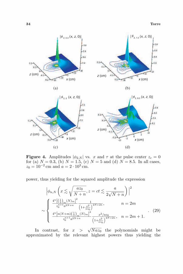
Figure 4. Amplitudes |φ2,N | vs. x and τ at the pulse center zc = 0for (a) N = 0.3, (b) N = 1.5, (c) N = 5 and (d) N = 8.5. In all cases,z0 = 10−2 cm and a = 2 · 103 cm.
power, thus yielding for the squared amplitude the expression
∣∣∣φn,N
(x .
√az0
N + n, z = ct . a
2√
N + n
) ∣∣∣2
∼
4n[( 12)m
(N)m]2
zn+10 a2N+n
1(1+ x2
az0
)2N+2n , n = 2m
4n[n(N+m)( 12)m
(N)m]2
zn+10 a2N+n
x2/az0(1+ x2
az0
)2N+2n , n = 2m + 1.
. (29)
In contrast, for x >√
Naz0 the polynomials might beapproximated by the relevant highest powers thus yielding the

Progress In Electromagnetics Research B, Vol. 16, 2009 35
expression∣∣∣∣φn, N
(x>
√Naz0, z=ct. a
2√
N+n
)∣∣∣∣2
∼ [(2N)n]2
z0a2N+2n
(x/√
az0
)n
(1+ x2
az0
)2N+2n. (30)
where the power xn mitigates the descending trend of the multi-Lorentzian factor (1 + x2
az0)−2N−2n.
Figures 3 and 4 show the surface plots and the correspondingcontour plots of the amplitudes |φn, N | vs. x and τ at the pulse centerzc = 0 respectively for n = 1 and n = 2 and different values of N . Inall cases, z0 = 10−2 cm and a = 2 · 103 cm. Again, the maximum ineach plot is normalized to unity.
We see that the shape of the plots changes rather significantlywith N . In fact, for n = 1 we observe, as expected, two identical lobesat each side of the central nodal line x = 0. For N = 0.1 the contourplot for each lobe exhibits an irregular rhombo-like shape, whereas anoverall 8-like shape in the (x, τ) plane is in contrast obtained for thecontour plot relevant to N = 0.5. Then, a butterfly-like shape pertainsto the case N = 1, which shape is further deformed with increasing N ,two lateral lobes more strongly emerging to each side with increasingN .
Likewise, for n = 2 one gets an almond-shaped contour plot witha predominant central lobe for N ≤ 1. The lateral lobes separatefrom the central one, becoming more evident indeed with increasingN up to N . 2.5. Then, for N > 2.5 they come to be re-absorbed inthe central lobe, which so displays a more complex structure, with anoverall four-petal flower-like appearance of the relevant contour plots.
Similar behaviors are observed for higher values of n, respectivelyodd and even, although the effect of N becomes evident for even higherN with increasing n.
Finally, in Fig. 5, we have plotted the peak amplitudes of theφn,N ’s at the pulse center z = ct vs. z for some values of n and Nwith the parameters z0 and a being set as before to z0 = 10−2 cm anda = 2 · 103 cm. The symbol x∗ appearing in the labels of the verticalaxis in the plots in Parts (c) and (d) denote the value of x, x∗(n, N), atwhich |φn, N (x, z = ct)| is maximum. Such maxima occur at x∗ = 0 foreven n, like n = 0 and n = 2 to which the graphs in Frames (a) and (b)of the figure pertain. In contrast, we found that the x∗’s accomodaterather well according to the relation
x∗(n = 1, N)[cm] ' 4.45(1.5N + 1)0.55
,

36 Torre
101
0.1
0.01
1 10-3
1 10-4
1 10-5
1 10-6
1 10-7
1 10-8
1 10 100 1 103
1 104
1 105
1 106
1 1071 10
8
|
(0,
z =
ct)
|0,
N0.1
0.01
1 10-3
1 10-4
1 10-5
1 10-6
1 10-7
1 10-8
|
(0, z
= c
t)|
2,N
1 10-9
1 10-10
1 10 100 1 103
1 104
1 105
1 106
z (cm) z (cm)
(a) (b)0.1
0.01
1 10-3
1 10-4
1 10-5
1 10-6
1 10-7
1 10-8
|
(x
, z
= c
t)|
1,N
1 10-9
0.10.01
1 10-3
1 10-4
1 10-5
1 10-6
1 10-7
1 10-8
|
(x
, z
= c
t)|
3,N 1 10
-9
1 10-10
1 10-13
1 10-12
1 10-11
z (cm) z (cm)
(c) (d)
1 10 100 1 103
1 104
1 105
1 106
1 10 100 1 103
1 104
1 105
1 106
* *
φ φφφ
.
.
.
.
.
.. . . . . .
.
.
.
.
.
.
.
.. . . .
.
.
.
.
.
.
.. . . .
.
.
.
.
.
.
.
.
.
.
.. . . .
Figure 5. Peak amplitudes |φn,N (x∗, z = ct)| vs. z for N = 0.1(solid line), 0.3 (dotted line), 0.5 (dashed line), 1 (dash-dotted line)and (a) n = 0, (b) n = 2, (c) n = 1 and (d) n = 3 with z0 = 10−2 cm,a = 2 · 103 cm.
for n = 1, and to
x∗(n = 3, N)[cm] ' 4.45(1.5N + 3)0.7
,
for n = 3. We recall that the odd n amplitudes at z = ct exhibit a twomain lobes structure.
The straight line in the plot of Part (a) of the figure (relevantto n = 0) reproduces a z−1-like decay, which as expected rules theamplitude for N = 1 at large values of z : z > 105 cm. Evidently theother plots in the same frames display a decay for large z slower thanz−1. Such a decay, which amounts to a power decay slower than theusual z−2, is reported in the literature as missilelike [34, 35]; it attractedinterest for possible applications in the transmission of information,which so might be very difficult to intercept or jam [34, 35]. As tothe plots in the other frames, we note that for n = 1 and n = 2, wedetect a peak amplitude decay respectively of ∼ z−0.91 and ∼ z−0.95
at N = 0.1, whilst decays roughly as or faster than z−1 pertain to the

Progress In Electromagnetics Research B, Vol. 16, 2009 37
peak amplitudes for N > 0.1. Finally, for n = 3 a decay faster than z−1
is displayed by the peak amplitudes for all the values of N consideredin the figure (for instance, as ∼ z−1.75 at N = 0.1). Evidently, theseconsiderations would gain a further practical interest once the practicallaunchability of the concerned wave functions could be demonstrated,but, as previously stressed, we will not dwell here on such an issue.
Before closing the section, we wish to note that the aboveintroduced solutions of the 2D wave equation frame within the class ofCourant-Hilbert solutions [36], which in general write as
u(x, y, z, t) = hf(θ). (31)
The waveform f is an arbitrary function of a single variable withcontinuous partial derivatives, whilst the phase function θ(x, y, z, t)and the attenuation (or distortion) factor h(x, y, z, t) are fixedfunctions. In particular, θ is any solution of the space-time eikonalequation (θx)2 + (θy)2 + (θz)2 − (θct)2 = 0.
Evidently, in the case of the 2D solutions φn,N ’s, the phase
θ(x, z, t) = σ +x2
τ − iz0, (32)
is just the 2D version of the Bateman-Hillion phase [4, 7], whereasthe relevant waveform f shapes as the power function fn,N (θ) =(θ + ia)−N−n and the attenuation factor is hn,N (x, z, t) ∝
(σ+ia)n2
(τ−iz0)n+1
2H
(N)n (XN (x, z, t)).
4. THE RELATIVISTIC HERMITE POLYNOMIALS ANDTHE 3D WAVE EQUATION
As recalled in Introduction, there are definite rules to constructsolutions of the 3D wave equation from those of the 2D one. Inparticular, we consider here the solutions of the 3D wave equation,un,N (x, y, z, t), obtained from the above introduced φn,N ’s accordingto the transformation (3), which so yields
u(±)n,N (x, y, z, t) = (x± iy)−
12 φn,N (r, z, t) = r−
12 e∓
i2ϕφn,N (r, z, t), (33)
where φn,N is given in Equation (25) and r, ϕ denote polar coordinatesin the x-y plane: r =
√x2 + y2, ϕ = arctan( y
x).Again, the interchange of σ and τ in (33) provide alternative
solutions of (1). Also, as previously recalled, replacing σ → 2z in

38 Torre
the wave functions yields the expressions of the corresponding pulsedbeams [31–33].
Evidently for any n the u(±)n,N ’s are not axisymmetric, even though
their amplitudes are.The u
(±)n,N ’s as well belong to the class (31) of Courant-Hilbert
solutions of the wave equation [36]. The relevant phase θ(x, y, z, t)is just the Bateman-Hillion axisymmetric phase, i.e., (32) with r inplace of x, the waveform shapes as before as fn,N (θ) = (θ + ia)−N−n,whereas the attenuation factor exhibits now the factor (x± iy)−
12 , i.e.,
h(±)n,N (x, y, z, t) ∝ (x± iy)−
12
(σ+ia)n2
(τ−iz0)n+1
2H
(N)n (XN (r, z, t)).
It is just due to such a factor that the u(±)n,N ’s might present
the fixed curve of singularities (x = 0, y = 0). This undeniablyoccurs for even n’s, whilst it is easy to see that for odd n’sh
(±)n,N (x, y, z, t) −−−−−−→
x→0, y→00. To avoid the singularity occurring for even
n’s, one may take ∂∂(x+iy)u
(+)n,N and ∂
∂(x−iy)u(−)n,N when n = 2m. As we
will see in the following, this amounts to consider only the odd-orderforms of (33), i.e., u
(±)2m+1,N .
Then, on account of the above illustrated behavior of theamplitudes |φn,N | at the pulse center (see Equations (29) and (41)),we see that
∣∣∣∣u(±)n,N
(x, y, z = ct . a
2√
N + n
)∣∣∣∣2
∼
4n[( 12)m
(N)m]2
zn+10 a2N+n
1/r(1+ r2
az0
)2N+2n , n = 2m
4n[n(N+m)( 12)m
(N)m]2
zn+3
20 a2N+n+1
2
r/√
az0(1+ r2
az0
)2N+2n , n = 2m + 1(34)
for r .√
az0N+n , whereas for r >
√Naz0
∣∣∣u(±)n,N
(x, y, z = ct . a
2√
N+n
)∣∣∣2∼ [(2N)n]2
z320 a2N+2n+ 1
2
(r/√
az0
)n−1
(1 + r2
az0
)2N+2n. (35)
As an example, Fig. 6 shows the contour plots of the amplitudes|u(±)
n,N | vs. r and z at the pulse center zc = 0 for some values of the

Progress In Electromagnetics Research B, Vol. 16, 2009 39
|u 1, 0.1 (r, z, 0)|+_( ) |u 1, 1.5 (r, z, 0)|
+_( )
z (
cm
)
z (
cm
)
r (cm) r (cm)
(a) (b)
|u 7, 0.1 (r, z, 0)|+_( )
|u 7, 10.5 (r, z, 0)|+_( )
z (
cm
)
r (cm)
z (
cm
)
r (cm)
(c) (d)
Figure 6. Contour plots of the amplitudes |u(±)n,N | vs. r and z at t = 0
for (a) n = 1, N = 0.1, (b) n = 1, N = 1.5, (c) n = 7, N = 0.1 and(d) n = 7, N = 10.5. In all cases, z0 = 10−2 cm and a = 2 · 103 cm.
parameter N and the order n (in particular odd according to the aboveconsiderations).
A numerical analysis of the cases in the figure has shown thatthe relative r-z amplitude distributions remain almost unaltered, apartfrom a sort of breathing (a smooth sequence of broadening and focusingmore evident along the z-direction at a rather irregular rate), up tot ≈ 10−9−10−8 s (basically depending on n and N , for the fixed valuesof z0 and a as in the cases of the figure). Then, such distributions startto change rather rapidly developing two more or less subtle “walls” alsodisplaying a somewhat articulated structure.
Let us note that, as in the previous figures, the values of thefree parameters z0 and a have been set to z0 = 0.01 cm and a =

40 Torre
2 · 103 cm and so z0 ¿ a. Therefore, according to the analysispresented in [17, 18], where the electromagnetic vector fields generatedby the wave function s1(x, y, z, t) = 1
(σ+ia)(τ−iz0)+r2 , taken as a Hertzpotential oriented both parallel [17] and orthogonal [18] to the z-direction have been studied in detail, the frames in the figures pertainto the paraxial regime (z0 ¿ a). So, it may be interesting to comparethe r-z amplitude behavior in the case z0 ¿ a and in the case z0 ≈ a.Fig. 7 shows indeed the r-z contour plots of the amplitudes |u(±)
n,N | forn = 5 and N = 2.1 at t = 0 and t > 0 for two sets of values of z0
and a, i.e., as before, z0 = 0.01 cm and a = 2 · 103 cm (z0 ¿ a) andz0 = 10 cm and a = 20 cm (z0 ≈ a).
|u 5, 2.1 (r, z, 0)|+_( ) |u 5, 2.1 (r, z, 10 )|+_( ) -8
z(c
m)
r (cm)
(a) (b)
z(c
m)
r (cm)
|u 5, 2.1 (r, z, 0)|+_( ) |u 5, 2.1 (r, z, 10 )|+_( ) -9
r (cm)
(c) (d)
r (cm)
z(c
m)
z(c
m)
Figure 7. Contour plots of the amplitudes |u(±)5,2.1| vs. r and z relative
to z0 = 10−2 cm and a = 2 · 103 cm at (a) t = 0 and (b) t = 10−8 s andto z0 = 10 cm and a = 20 cm at (c) t = 0 and (d) t = 10−9 s.

Progress In Electromagnetics Research B, Vol. 16, 2009 41
5. HERMITE-LORENTZIAN WAVE FUNCTIONS:RELATION TO THE LAGUERRE-LORENTZIAN WAVEFUNCTIONS
As mentioned earlier, the splash pulses (6) are solutions of the 3Dwave equation. In particular, considering exponents δ > 0, one couldunderstand the relevant splash pulses as the 3D counterpart of theφ0,N ’s with the cartesian coordinate x replaced by the radial one r,and the further multiplication by the factor 1√
τ−iz0. In symbols, with
δ = N in (6) one has
sN (x, y, z, t) =1√
τ − iz0φ0,N (r, z, t). (36)
Of course, in order that the above could convey a rule to constructsolutions of the 3D wave equation from those of the 2D wave equation,namely,
φ(x, z, t) → v(x, y, z, t) =1√
τ − iz0φ(r, z, t), (37)
the 2D solution φ(x, z, t) must satisfy the equation[
∂
∂x− 2x
τ − iz0
∂
∂σ
]φ(x, z, t) = 0. (38)
The above is evidently satisfied by the φ0,N ’s for any N , and henceby (37) one gets the splash pulses (36).
On passing we may note that Equation (38) is satisfied bythe 2D Gaussian pulse φG(x, z, t) = 1√
τ−iz0eikθ(x,z,t) as well as
by the 2D modified-power-spectrum (MPS) pulse φMPS(x, z, t) =1√
τ−iz0
1(θ+ia)q eikθ(x,z,t), from which indeed through (37) one respec-
tively gets the 3D Gaussian and MPS pulses [24], the latter combiningboth the Gaussian and splash-pulse waveforms.
As previously recalled, the splash pulses have been reconsideredin [19] in the form
v0,N (r, z, t) =1
τ − iz0
(σ + ia +
r2
τ − iz0
)−N− 12
, (39)
i.e., for exponents δ > 12 . This was functional to the possibility of
conveniently relating some higher-order solutions vn,l,N (x, y, z, t) to theRLPs (20). Such solutions are generated by repeatedly acting on (39)

42 Torre
by the operators L±
L±(x, y) =∂
∂x± i
∂
∂y= e±iϕ
(∂
∂r± i
r
∂
∂ϕ
)= 2
∂
∂(x∓ iy). (40)
Since L+L− = L−L+ = ∂2
∂x2 + ∂2
∂y2 and [ ∂∂σ,τ , L±] = 0, it is evident that
vn,l,N (x, y, z, t) = Ln+Ln+l
− v0,N (r, z, t) (41)
is a solution of the 3D wave equation for values of the integers nand l, respectively addressed as radial and angular indices, such thatn ≥ 0 and l ≥ −n. Specifically, in [19] the axisymmetric solutionsgenerated from the scheme (41) with l = 0, in which case: Ln
+Ln− =[∇2
r]n, have been discussed in detail, and there related, as mentioned
earlier, to the RLPs, which in fact act as modulating factors of theaxisymmetric Lorentzian-like wave functions (39), whose exponent isfurther increased to N + 2n + 1
2 .In the same vein, we may ask whether the above introduced
Hermite-Lorentzian solutions of the 3D wave equation u(±)n,N (x, y, z, t),
being obtained through (3) from the higher-order Hermite-Lorentziansolutions φn,N (x, z, t) of the 2D wave equation, might be understoodas higher-order solutions relatively to certain fundamental ones,which could reasonably be guessed to be u
(±)0,N (x, y, z, t) = (x ±
iy)−12 φ0,N (r, z, t). In other words, we may ask whether it is possible
to identify a sort of generation scheme for the u(±)n,N ’s as
u(±)j(m),N (x, y, z, t) = Vm
± u(±)0,N (x, y, z, t),
for some fundamental solutions u(±)0,N (x, y, z, t). The order j of the
resulting functions may in general depend in some way on the powerm (> 0), to which the generation operators V± (practically, symmetryoperators of the wave equation) are rised up.
In this connection, it is easy to verify that
L+u(+)n,N = u
(−)n+1,N , L−u
(−)n,N = u
(+)n+1,N ,
L+L−u(+)n,N = u
(+)n+2,N , L+L−u
(−)n,N = u
(−)n+2,N .
(42)
Then, considering the two sets of functions u(+)n,N and u
(−)n,N we may
say that elements in the same set are connected by steps of 2 in therelative orders by the transverse Laplacian L+L−, whereas elements in

Progress In Electromagnetics Research B, Vol. 16, 2009 43
the two sets are connected by steps of 1 in the relative orders by L+
and L−, respectively bridging the u(+)n,N ’s to the u
(−)n,N ’s and vice versa.
So, as noted earlier, taking the solutions L+u(+)2m,N and L−u
(−)2m,N one
can avoid the singularity associated with the even-order forms of (33)simply because so doing one picks up only the odd-order forms of (33).
According to (42), we may generate elements in each set applyingL+L− to u
(±)0,N and to u
(±)1,N , which so turn respectively into the even and
odd order solutions u(±)2m,N and u
(±)2m+1,N . In other word, the even and
odd order solutions, u(±)2m,N and u
(±)2m+1,N , arise from different paths,
one originating from u(±)0,N the other from u
(±)1,N :
[L+L−
]mu
(±)0,N = u
(±)2m,N ,
[L+L−
]mu
(±)1,N = u
(±)2m+1,N . (43)
Furthermore, a more compact scheme can be identified, whichwill also clarify the link of the u
(±)n,N ’s with the 3D solution (39) and its
higher order versions (41), considered in detail, as already mentioned,in [19].
In fact, taking into account the relations (19) between the RHPsand the RLPs and the formal expressions
Ln+Ln+l
−
(1+
r2
N
)−N− 12
= (−)n+l22n+ln!Γ(N+ 1
2 +n+l)
Γ(N + 1
2
)Nn+l
rle−ilϕL(l,N)n
(r2
)
(1+
r2
N
)−N−2n−l− 1
2 , n ≥ 0, l ≥ −n, (44)
after some algebra we end up with the generation scheme for the u(±)n,N ’s
u(±)n,N (x, y, z, t) = L
n2∓L
n−12± v0,N (r, z, t), (45)
involving the splash pulses (39).Evidently, the above for n = 0 allows one to relate the rule (3) in
the case of the v0,N ’s to the symmetry operators L± (rised to ±12) of
the wave equation.We note that according to whether the order n is even or odd
the power ±12 of the operators L± is involved in (45). The effect of
L±12± can be proved to be in accord with the general relation (44), on
account of the operational rule for negative powers of operators [37]
A−p =1
Γ(p)
∫ ∞
0dssp−1e−sA, p ∈ R+.

44 Torre
The above yields in fact for the operators of our concern the expression
L−12± =
1Γ
(12
)∫ ∞
0dss−
12 e−sL± ,
which explicitly amounts to
L−12± ψ(x, y) =
1√π
∫ ∞
0dss−
12 ψ(x− s, y ∓ is),
and hence to
L12±ψ(x, y)= L±L−
12± ψ(x, y)=
1√π
∫ ∞
0dss−
12
[L±ψ
](x−s, y∓is).
The direct application of the above rules to v0,N (r, z, t) yields therelations (45).
Interestingly, the Hermite-Lorentzian solutions of the 3D waveequation appear to be generated by repeated applications of half-integer powers of the operators L± to the fundamental axisymmetricLorentzian-like solution — or splash pulse — v0,N . In other words, wemay say that the u
(±)n,N ’s can be constructed by the same scheme (41)
through which the Laguerre-Lorentzian solutions are generated, butwith l = ±1
2 , the orders of the involved RHPs in the resulting functionsbeing accordingly odd or even. In a sense, the u
(±)n,N ’s can be regarded
as higher-order Laguerre-Lorentzian solutions of the 3D wave equation(or, higher-order splash pulses) corresponding to fractional azimuthalorders, specifically ±1
2 .Needless to say, relations (45) are in accord with (42).
Furthermore, as conveyed by (42) and (43), applying L+, L− or L+L−yields further solutions of the wave equation. Interestingly, one canget “compact” forms through the schemes
Lm+u
(+)0,N −→ (x + iy)m
(τ − iz0)mu
(+)0,N+m,
Lm−u
(−)0,N −→ (x− iy)m
(τ − iz0)mu
(−)0,N+m,
(46)
which conform to the rule that, if v is a solution of the wave equation,also (x±iy)m
(τ−iz0)m v is a solution [8] (set N −m in (46)), provided that[L± − 2
x + iy
τ − iz0
∂
∂σ
]v = 0,

Progress In Electromagnetics Research B, Vol. 16, 2009 45
the latter appearing as the 2D complexified version of (38).As a final note, let us say that the transformations signified by (4)
may be framed within the same scheme above discussed, resortingof course to symmetry operators that involve both space and timecoordinates, i.e., replacing L± by T± = ∂
∂x ± i ∂∂y with y = ict.
6. LORENTZIAN-LIKE WAVE FUNCTIONS ANDKLEIN-GORDON EQUATION
Strictly related to the question of the solutions to the wave equationhas always been considered that of the solutions to the Klein-Gordonequation. Several approaches have been devised in this connectionyielding both particular, i.e., valid under specific hypotheses and/orapproximations, and general solutions of the latter [10, 11, 13, 24, 38–42]. Here, we simply deduce solutions to the Klein-Gordon equationwhich may be put in relation with the Lorentzian-like wave functions,illustrated in the previous sections.
As observed in [42], we may obtain possible solutions to the 3DKlein-Gordon equation
[∇2 − c−2∂2
t −(mc
~
)2]
u(x, y, z, t) = 0, (47)
through the 1D Fourier transform of those of a 4D homogeneous waveequation, just evaluated at Ω = mc
~ . In symbols, we can write
u(x, y, z, t) =∫ +∞
−∞dζe−iΩζu(x, y, ζ, z, t)
∣∣∣∣Ω=mc
~
, (48)
where u(x, y, z, ζ, t) solves the 4D homogeneous scalar wave equation[∇2 + ∂2
ζ − c−2∂2t
]u(x, y, ζ, z, t) = 0, (49)
or, in terms of the characteristic variables τ = z − ct and σ = z + ct,[∂2
x + ∂2y + ∂2
ζ + 4∂σ∂τ
]u(x, y, ζ, z, t) = 0. (50)
In the sequel we will in general address the constant term enteringthe Klein-Gordon equation, which of course specifies in accord withthe physical context of concern, as Ω2 (in particular, Ω = mc
~ in (47),which in fact describes the dynamics of a relativistic massive particlewith spin zero).
The usefulness of (48) stems evidently from the possibility ofobtaining explicit forms of the Fourier integral for specific expressions

46 Torre
of u(x, y, ζ, z, t). In [42], for instance, it has been applied to suitablesuperpositions of Gaussian pulses in order to obtain what are therereferred to as Gaussian packets for the Klein-Gordon equation in thecase of both two and three space-variables.
Here we retain the axisymmetric Lorentzian-like form of thesolutions to the wave equation, we dealt before, and hence we take
Uδ(x, y, ζ, z, t) =1
(τ − iz0)32
(σ + ia +
x2 + y2 + ζ2
τ − iz0
)−δ
(51)
which evidently solves (50) for any δ.The above conforms to the general rule stated firstly in [21]
and later re-derived in [10], concerning the relatively distortion-freesolutions of the scalar wave equation of arbitrary (space) dimensionm > 1. Accordingly, (51) is the 4D counterpart of sδ in (6), whichsolves the 3D wave equation.
Then, on account of the integral (3.385.9) of [44], we can evaluatethe Fourier integral in (48) in the specific case of (51) (see also (16)),thus obtaining the axisymmetric solution of (48) as
uδ(x, y, z, t) = (τ − iz0)δ− 3
21
βδ(x, y, z, t)W0, 1
2−δ(2Ωβ), (52)
where Wκ,µ denotes Whittaker’s second function [30] and
β(x, y, z, t) =√
(τ − iz0) (σ + ia) + r2. (53)
Note that β =√
s1, s1 being given in (6).According to the condition for the applicability of (3.385.9) of [44],
expression (52), as derived from (48) with (51), should hold underthe conditions that Re(β) > 0 and δ > 1
2 . Actually, a direct checkassures that (52) solves (47) without any constraint on β and/or δ.In particular, (52) holds for δ = 0 as well, which evidently yields therather trivial solutions 1
(τ−iz0)32
and 1
(σ+ia)32
of (49), whose link to the
splash-like wave functions is hardly recognizable.We also note that interchanging τ and σ in (52) will provide
alternative solutions of the Klein-Gordon equation, whose pulsed beamsolutions follow from the known replacement σ → 2z.
We recall here the symmetry properties of Whittaker’s secondfunction with respect to the change of sign of its indices, namely, [30]
Wκ,µ(z) = Wκ,−µ(z), W−κ,µ(−z) = W−κ,−µ(−z),

Progress In Electromagnetics Research B, Vol. 16, 2009 47
as well as its relation to the modified Bessel function of second kindKµ — already recalled in Section 2 — and consequently to the Hankelfunctions H
(1)µ , H
(2)µ :
W0,µ(z) =√
z
πKµ
(z2
)=
i√
πz
2e−iµ π
2 H(1)µ
(iz
2
),
W0,µ(iz) =√
πz
2e−i π
4(1+2µ)H(2)
µ
(z
2
).
It may also be interesting to report the relation of W0,µ(z) to theordinary Laguerre polynomials L
(α)n in correspondence of specific
determinations of the second index µ [45], i.e.,
W0, 12+n(z) = (−)nn!z−ne−
z2 L(−2n−1)
n (z),
which applies to our case when δ = j, with j positive integer.In particular, for δ = 0 and δ = 1 one obtains in (52) W0, 1
2
which simply implies an exponential function since W0, 12(z) = e−
z2 .
Therefore,
u0(x, y, z, t) =1
(τ − iz0)32
e−Ω√
(τ−iz0)(σ+ia)+r2,
u1(x, y, z, t) = s 12(x, y, z, t)e−Ω
√(τ−iz0)(σ+ia)+r2
,
(54)
with s 12
being the splash pulse (6).Figure 8 shows the 3D surface plots of the real and imaginary parts
of u0, u1 and u 32
— apart from unessential multiplicative constants— vs. r and z at ct = 0 and ct = 10, the free parameters beingset to z0 = 10−1 and a = 20. The oversigned symbols denote therespective quantity normalized to 1
Ω . Note that the vertical scales inthe graphs have minor meaning since, in order to show both the realand imaginary parts in the same frame, the surface plots of the formerhave been shifted upward, the flat part of the relative surfaces actuallycorresponding to zero. We may see a certain localization of both thereal and imaginary parts of the uδ’s at a minor extent when increasingδ.
Interestingly, an expression similar to that for u1(x, y, z, t) hasbeen obtained in [40] (see Equation (11) there with a1 = a3) froma suitable weighted superposition over a free parameter of the focuswave mode solution of (47). In a sense, the expression (48) can be seenas a weighted superposition of what can be considered as solutions of

48 Torre
(r, z, 0)_ _
0 (r, z, 10)_ _
0
z_ r
_
z_
r_
(a) (b)
_ _1
_ _1
z_ r
_
z_
r_
(c) (d)_ _ _ _
z_ r
_
z_
r_
(e) (f)
2_3
2_3
u
(r, z, 0)u
u
(r, z, 10)u
(r, z, 10)u (r, z, 0)u
Figure 8. 3D plots of the real (upper surfaces) and imaginary parts(lower surfaces) of (a), (b) u0, (c), (d) u1 and (e), (f) u 3
2vs. r and z at
ct = 0 and ct = 10, the third argument of the u’s being here ct. In allgraphs, z0 = 10−1 and a = 20.

Progress In Electromagnetics Research B, Vol. 16, 2009 49
the 3D wave equation over the free parameter ζ, with the weightingfunction being just the simple harmonic e−iΩζ .
It is evident that the solutions of the 2D scalar wave equationdeduced in Section 3 in the form (25) can be used to obtain solutionsof the 1D Klein-Gordon equation [∂2
z − c−2∂2t ]u(z, t) = 0. According to
the properties of the Fourier integral, we see that the φn,N ’s, apart fromunessential multiplying constants that involve powers of Ω, basicallyyield the same function, which in fact writes
uN (z, t) =(τ − iz0)
N−12
(σ + ia)N2
W0, 12−N
(2Ω
√(τ − iz0) (σ + ia)
). (55)
In Section 3, we limited ourselves to consider N > 0; thiswas functional to the possibility of introducing higher-order solutionsrelated to the RHPs, whose definition implies N > 0. Of course, sucha constraint here has no sense, so we can consider the case N = 0,which, as noted before, yields the trivial solutions 1√
τ−iz0and 1√
σ+iaof
the 2D wave equation. In that case, one obtains W0, 12
in (55) just aswith N = 1. In fact, the solutions corresponding to N = 0 and N = 1differ only for the multiplying factor, involving τ − iz0 in the formercase and σ + ia in the latter case. Explicitly, we have
u0(z, t) =1√
τ − iz0e−Ω
√(τ−iz0)(σ+ia),
u1(z, t) =1√
σ + iae−Ω
√(τ−iz0)(σ+ia),
(56)
in practice obtained one from the other by interchanging the termsτ − iz0 and σ + ia.
In Fig. 9, we show the z-profiles of the real and imaginary partsof u0 and u1 as well as of the relative amplitudes at ct = 0 andct = 10. As in the figures above, the coordinates as well as the variousparameters are normalized to 1
Ω . As it can easily be inferred from therespective expressions, one basic difference between u0 and u1 is thatthe amplitude of u1 decreases more quickly with z than that of u0.
In conclusion, we may say that, in accord with the recipe (48),solutions of a m-dimensional Klein-Gordon equation generated bysplash-like pulses write as (xm ≡ z)
uδ(x1, . . . , xm−1, z, t)
= (τ−iz0)δ−m
21
βδ(x1, . . . , xm−1, z, t)W0, 1
2−δ(2Ωβ), (57)

50 Torre
0
_ (z, 10)
0
_
z_
z_
(a) (b)
(z, 0)1
_
1
_
z_
z_
(c) (d)
u
(z, 0)u u
(z, 10)u
Figure 9. z-profiles of the real parts (solid line), imaginary parts(dot-dashed line) and of the amplitudes (white diamonds) of (a), (b)u0 and (c), (d) u1 at ct = 0 and ct = 10, the third argument of the u’sbeing here ct. In all graphs, z0 = 10−2 and a = 102.
with the m-dimensional version of β being evidently
β(x1, . . . , xm−1, z, t) =
√√√√(τ − iz0) (σ + ia) +m−1∑
j=1
x2j . (58)
More in general, let us say that non-axisymmetric forms for thesplash pulses may be considered, like, for instance, in the case of m+1
Progress In Electromagnetics Research B, Vol. 16, 2009 51
space variables
Uδ(x1, . . . , xm−1, ζ, z, t)=1√
(τ − iz0)(τ − iz1) . . . (τ − izm−1)(
σ+ia+x2
1
τ − iz1+. . .+
x2m−1
τ − izm−1+
ζ2
τ − iz0
)−δ
, (59)
which so yields the (m + 1)-arbitrary constant dependent expression
uδ(x1, . . . , xm−1, z, t)
=(τ − iz0)
δ− 12√
(τ − iz1) . . . (τ − izm−1)1
βδ(x1, . . . , xm−1, z, t)W0, 1
2−δ(2Ωβ), (60)
with
β(x1, · · · , xm−1, z, t) =
√√√√√(τ − iz0)
(σ + ia) +
m−1∑
j=1
x2j
τ − izj
, (61)
as a possible solution to a m-dimensional Klein-Gordon equation.We close the section noting that the expression for u1(z, t) in (56)
has been obtained in [40] as well (see Equation (23) there settinga1 = a3), where it has been used to construct a solution to the3D Klein-Gordon equation, i.e., u1(x, y, z, t) in (54), according tothe method outlined in that reference. Evidently, inspecting therelations (60) and (61) we may recover within the present context therule stated in [40], namely that one can pass from solutions of the 1DKlein-Gordon equation to solutions of the 3D equation, multiplyingthe expression (55) of the 1D solution by the factor 1∏m−1
j=1
√τ−izj
and
replacing in it the characteristic variable σ = z + ct ≡ σ1D by
σ1D = z + ct → σmD = σ1D +m−1∑
j=1
x2j
τ − izj.
It is easy to write down the alternative expressions in which theroles of the characteristic variables τ and σ are interchanged. Thus,for instance, with m = 2 (and σ ↔ τ) in (60) and (61), one mayrecover the expression of the Gaussian packet for the 2D Klein-Gordonequation deduced in [42] (see Equation (14) there, with in particularthe various parameters being set as ν = −δ, σ = 0 and ε1 = ε2.)

52 Torre
7. CONCLUSION
In [19] solutions of the free-space 3D scalar wave equation have beensuggested, which resort to the splash pulses and have the RLPs asmodulating factors of the basic splash-pulse waveform. A definitegeneration scheme for such solutions — referred to as Laguerre-Lorentzian solutions — have been deduced, which parallels thatholding for the Laguerre-Gaussian pulses; both indeed are based onthe same symmetry operators L± of the wave equation.
Paralleling the analysis developed in [19], we have considered heresolutions of the 2D scalar wave equation, which can be regarded as the2D versions of the wave functions investigated in the aforementionedpaper. In fact, these solutions involve the RHPs as modulating factorsof what can be regarded as the 2D version of the basic splash-pulsewaveform.
It has been recalled that the RHPs have been introduced aspolynomial component of the quantum relativistic 1D harmonicoscillator wave function [25]. It has also been recalled that theyhave been recently re-considered within the context of the paraxialwave propagation in [26], where an “optical interpretation” of theHermite-Lorentzian functions Φ(N)
n has been suggested, enlighteningtheir relation with the Lorentz beams, i.e., beams described by fieldsdisplaying a spatial dependence at the plane z = 0 of the type 1
1+x2 .The latter have been introduced in [46] on the basis of the experimentalobservations reported in [47, 48].
Then, applying the rule (3), from the obtained 2D wave functionsfurther solutions of the 3D wave equation — referred to as Hermite-Lorentzian solutions — have been constructed, which finally have beenframed within the same generation scheme, that holds for the Laguerre-Lorentzian solutions, involving in fact the same operators L± althoughthrough fractional, besides integer, powers.
As stressed in the Introduction, in our opinion, the unifyingview — that emerges from the analysis here presented — of the3D wave equation solutions of the splash-pulse type, deduced in thepaper and in the previous quoted reference, is of interest at leastfrom a mathematical viewpoint. As also stressed in the Introduction,in fact, we do not dwell here on the practical feasibility of thesolutions that have been suggested, which evidently demand for furtherinvestigations.
In this regard, however, we simply recall that following theoriginal hint, illustrated in detail in [24], an accurate analysis ofthe correspondence between source-free and aperture-generated MPS,splash and DEX pulses has been carried out in [16]. In particular, as

Progress In Electromagnetics Research B, Vol. 16, 2009 53
a result of such an analysis, the launchability of the splash pulses (atleast for the values of the exponent δ considered in the paper) has beendemonstrated to be possible with a maintenance of the features of thesource-free field over a rather extended z-range between the near- andthe far-field regions. The launching process, as described in [24], isbased on the Huygens construction yielding the scalar field generatedinto z > 0 half-plane by the source aperture from the relevant initialexcitation.
Accordingly, whereas the launchability of the v0,N ’s could bereasonably be assumed on account of the afore mentioned resultsin [16], we should face the issue concerning the launchability of theu
(±)n,N ’s.
It has also been recalled in the Introduction that in [18] theparaxial fields generated by s1(x, y, z, t) = 1
(σ+ia)(τ−iz0)+r2 taken asa Hertz potential oriented transversely to the direction of propagationhave been demonstrated to be the natural spatiotemporal modes of acavity resonator, thus suggesting their production could be achievedby exciting a curved mirror resonator or the equivalent lens waveguide.
Finally, explicit expressions for the solutions of the Klein-Gordonequation, which in a sense can be considered as generated from theLorentzian-like wave functions here discussed, have been deduced, alsoevidencing the relations with pertinent results already existing in theliterature.
ACKNOWLEDGMENT
The author is pleased to acknowledge interesting discussions withProfessor W. A. B. Evans, Dr. O. El Gawhary and Dr. S. Severini.
REFERENCES
1. Volterra, V., “Sur les vibrations des corps elastiques isotropes,”Acta Math., Vol. 18, 161–232, 1894.
2. Bateman, H., “The conformal transformations of a space offour dimensions and their applications to geometrical optics,”Proc. London Math. Soc., Vol. 2, 70–89, 1909.
3. Bateman, H., “The transformations of the electrodynamicalequations,” Proc. London Math. Soc., Vol. 8, 223–264, 1910.
4. Bateman, H., The Mathematical Analysis of Electrical and OpticalWave-motion on the Basis of Maxwell’s Equations, Dover, NewYork, 1955.

54 Torre
5. Miller, W., Symmetry and Separation of Variables, Addison-Wesley, Reading, MA, 1977.
6. Hillion, P., “The Courant-Hilbert solution of the wave equation,”J. Math. Phys., Vol. 33, 2749–2753, 1992.
7. Hillion, P., “Generalized phases and nondispersive waves,” ActaAppl. Math., Vol. 30, 35–45, 1993.
8. Borisov, V. V. and A. B. Utkin, “Generalization of Brittingham’slocalized solutions to the wave equation,” Eur. Phys. J. B, Vol. 21,477–480, 2001.
9. Kiselev, A. P., “Generalization of Bateman-Hillion progressivewave and Bessel-Gauss pulse solutions of the wave equation via aseparation of variables,” J. Phys. A: Math. Gen., Vol. 36, L345–L349, 2003.
10. Besieris, I. M., A. M. Shaarawi, and A. M. Attiya, “Bateman con-formal transformations within the framework of the bidirectionalspectral representation,” Progress In Electromagnetics Research,PIER 48, 201–231, 2004.
11. Besieris, I. M., A. M. Shaarawi, and R. W. Ziolkowski, “Abidirectional traveling plane wave representation of exact solutionsof the wave equation,” J. Math. Phys., Vol. 30, 1254–1269, 1989.
12. Kiselev, A. P., “Relatively undistorted waves. New examples,”J. Math. Sci., Vol. 117, 3945–3946, 2003.
13. Ziolkowski, R. W., “Exact solutions of the wave equation withcomplex source locations,” J. Math. Phys., Vol. 26, 861–863, 1985.
14. Hillion, P., “Splash wave modes in homogeneous Maxwell’sequations,” Journal of Elecromagnetic Waves and Applications,Vol. 2, 725–739, 1988.
15. Besieris, I. M., M. Abdel-Rahman, A. Shaarawi, andA. Chatzipetros, “Two fundamental representations of localizedpulse solutions to the scalar wave equation,” Progress In Electro-magnetics Research, PIER 19, 1–48, 1998.
16. Shaarawi, A. M., M. A. Maged, I. M. Besieris, and E. Hashish,“Localized pulses exhibiting a missilelike slow decay,” JOSA,Vol. 23, 2039–2052, 2006.
17. Hellwarth, R. W. and P. Nouchi, “Focused one-cycle electromag-netic pulses,” Phys. Rev. E, Vol. 58, 889–895, 1996.
18. Feng, S., H. G. Winful, and R. W. Hellwarth, “Spatiotem-poral evolution of focused singlecycle electromagnetic pulses,”Phys. Rev. E, Vol. 59, 4630–4649, 1999.
19. Torre, A., “Relativistic Laguerre polynomials and the splashpulses,” Progress In Electromagnetics Research B, Vol. 13, 329–

Progress In Electromagnetics Research B, Vol. 16, 2009 55
356, 2009.20. Brittingham, J. N., “Packetlike solutions of the homogeneous-
wave equation,” J. Appl. Phys., Vol. 54, 1179–1189, 1983.21. Kiselev, A. P., “Modulated Gaussian beams,” Radiophys. Quan-
tum Electron., Vol. 26, 755–761, 1983.22. Belanger, P. A., “Packetlike solutions of the homogeneous-wave
equation,” JOSA A, Vol. 1, 723–724, 1984.23. Sezginer, A., “A general formulation of focus wave modes,”
J. Appl. Phys., Vol. 57, 678–683, 1985.24. Ziolkowski, R. W., “Localized transmission of electromagnetic
energy,” Phys. Rev. A, Vol. 39, 2005–2033, 1989.25. Aldaya, V., J. Bisquert, and J. Navarro-Salas, “The quantum rel-
ativistic harmonic oscillator: Generalized Hermite polynomials,”Phys. Lett. A, Vol. 156, 381–385, 1991.
26. Torre, A., W. A. B. Evans, O. El Gawhary, and S. Severini,“Relativistic Hermite polynomials and Lorentz beams,” J. Opt. A:Pure Appl. Opt., Vol. 10, 115007, 2008.
27. Natalini, P., “The relativistic Laguerre polynomials,”Rend. Matematica, Ser. VII, Vol. 16, 299–313, 1996.
28. Nagel, B., “The relativistic Hermite polynomial is a Gegenbauerpolynomial,” J. Math. Phys., Vol. 35, 1549–1554, 1994.
29. Ismail, M. E. H., “Relativistic orthogonal polynomials are Jacobipolynomials,” J. Phys. A: Math. Gen., Vol. 29, 3199–3202, 1996.
30. Erdelyi, A., W. Magnus, F. Oberhettinger, and F. G. Tricomi,Higher Transcendental Functions, Vols. 1 and 2, MacGraw-Hill,New York, London and Toronto, 1953.
31. Heyman, E., “Pulsed beam propagation in inhomogeneousmedium,” IEEE Trans. Antennas Prop., Vol. 42, 311–319, 1994.
32. Hillion, P., “A remark on the paraxial equation for scalar wavesin homogeneous media,” Opt. Comm., Vol. 98, 217–219, 1993.
33. Hillion, P., “Paraxial Maxwell’s equation,” Opt. Comm., Vol. 107,327–330, 1994.
34. Wu, T. T., “Electromagnetic missiles,” J. Appl. Phys., Vol. 57,2370–2373, 1985.
35. Shen, H.-M. and T. T. Wu, “The properties of the electromagneticmissile,” J. Appl. Phys., Vol. 66, 4025–4034, 1989.
36. Courant, R. and D. Hilbert, Methods of Mathematical Physics,Vol. 2, Interscience, New York, 1962.
37. Srivastava, H. M. and H. L. Manocha, A Treatise on GeneratingFunctions, John Wiley and Sons, NY, 1984.

56 Torre
38. Shaarawi, A. M., I. M. Besieris, and R. W. Ziolkowski, “A novelapproach to synthesis of nondispersive wave packet solutions tothe Klein-Gordon and Dirac equations,” J. Math. Phys., Vol. 31,2511–2519, 1990.
39. Donnelly, R. and R. Ziolkowski, “A method for constructingsolutions of homogeneous partial differential equations: Localizedwaves,” Proc. R. Soc. London A, Vol. 437, 673–692, 1992.
40. Besieris, I. M., A. M. Shaarawi, and M. P. Ligthart, “A noteon dimension reduction and finite energy localized wave solutionsto the Klein-Gordon and scalar wave equations. I. FWM-type,”Journal of Electromagnetic Waves and Applications, Vol. 14, 593–610, 2000.
41. Besieris, I. M., A. M. Shaarawi, and M. P. Ligthart, “A noteon dimension reduction and finite energy localized wave solutionsto the Klein-Gordon and scalar wave equations. I. X wave-type,”Progress In Electromagnetics Research, PIER 27, 357–365, 2000.
42. Perel, M. V. and I. V. Fialkovsky, “Exponentially localizedsolutions of the Klein-Gordon equation,” J. Math. Sci., Vol. 117,3994–4000, 2003.
43. Kiselev, A. P. and M. V. Perel, “Relatively distortion-free wavesfor the m-dimensional wave equation,” Diff. Eq., Vol. 38, 1206–1207, 2002.
44. Gradshteyn, I. S. and I. M. Ryzhik, Table of Integrals, Series andProducts, 7th Edition, Academic Press, New York, 2007.
45. Buccholz, H., The Confluent Hypergeometric Function, Springer-Verlag, Berlin, 1969.
46. El Gawhary, O. and S. Severini, “Lorentz beams and symmetryproperties in paraxial optics,” J. Opt. A: Pure Appl. Opt., Vol. 8,409–414, 2006.
47. Dumke, W. P., “The angular beam divergence in double-heterojunction lasers with very thin active regions,” IEEEJ. Quantum Electron., Vol. 11, 400–402, 1975.
48. Naqwi, A. and F. Durst, “Focusing of diode laser beams: A simplemathematical model,” Appl. Opt., Vol. 29, 1780–1785, 1990.