PO

LIT

ICA

L E

CO

NO

MY

R

ESEA

RC

H IN

ST

ITU

TE

The Relative Income Theory of Consumption: A Synthetic

Keynes-Duesenberry-Friedman Model

Thomas I. Palley

April 2008

WORKINGPAPER SERIES

Number 170

Gordon Hall

418 North Pleasant Street

Amherst, MA 01002

Phone: 413.545.6355

Fax: 413.577.0261

peri@econs.umass.edu

www.peri.umass.edu

The Relative Income Theory of Consumption: A Synthetic Keynes-Duesenberry-Friedman Model

Abstract This paper presents a theoretical model of consumption behavior that synthesizes the seminal contributions of Keynes (1936), Friedman (1956) and Duesenberry (1948). The model is labeled a “relative permanent income” theory of consumption. The key feature is that the share of permanent income devoted to consumption is a negative function of household relative permanent income. The model generates patterns of consumption spending consistent with both long-run time series data and modern empirical findings that high-income households have a higher propensity to save. It also explains why consumption inequality is less than income inequality. JEL ref.: E3 Keywords: Consumption, permanent income, relative income, Keynes, Duesenberry, Friedman.

December 2007

1

I Introduction After World War II the theory of consumption became a central focus of research in

macroeconomics. With consumption spending making up approximately two-thirds of

peacetime GDP and with economists fearful that the economy would fall back into a

condition of mass unemployment, this focus was natural.

Initially, thinking was dominated by Keynes’ theory of the aggregate

consumption function that he had developed in his General Theory (1936). According to

Keynes’s theory, aggregate consumption was a positive but diminishing function of

aggregate income.

James Duesenberry’s 1949 book, Income, Saving and the Theory of Consumer

Behavior, challenged Keynes’ construction of consumption behavior by introducing

psychological factors associated with habit formation and social interdependencies based

on relative income concerns. This emphasis on the social dimensions of consumption had

a long history in institutional economics (Clark, 1918; Downey, 1910; knight, 1925a,

1925b; Mitchell, 1910; Patten, 1889; Veblen, 1899, 1909) and Duesenberry’s work

therefore promised to link Keynesian and institutional analysis.

However, in the 1950s Duesenberry’s theory of consumption was displaced by

Modigliani and Brumberg’s (1954) lifecycle theory of consumption and Friedman’s

(1957) permanent income hypothesis. These latter theories stripped consumption theory

of social interdependency and restored an atomistic approach that emphasized utility

maximization without regard for social concerns.1

1 Mason (2000) has examined the history of Duesenberry’s theory of consumption within the economics profession.

2

Over the last decade there has been a revival of interest in Duesenberry’s and

Veblen’s ideas on relative consumption and conspicuous consumption. This new research

has been primarily sociological and microeconomic in focus. Schor (2007) criticizes the

conventional model of utility on which conventional consumption theory is based as too

passive and simple in its motivations, and contrasts it with the thinking of Veblen,

Galbraith, and the Frankfurt school. Bagwell and Bernheim (1996) construct a utility

theoretic model of conspicuous consumption in which consumption of conspicuous goods

performs a signaling function that lets others know about individuals’ wealth. Empirical

work by Easterlin (1974, 1995) finds that relative income is the dominant determinant of

happiness. Experimental work by Alpizar et al. (2006) also confirms that relative income

and consumption matter for people. At the policy level, this microeconomic work

provides an efficiency justification for progressive taxation (Boskin and Sheshinski,

1978; Ireland, 2001) and taxation of luxury goods (Bagwell and Bernheim, 1996).

The above research is microeconomic in character. The current paper is

macroeconomic in character and focuses on aggregate consumption, which was the

primary focus of Duesenberry’s (1949) original work. The paper develops a simple

tractable model and diagrammatic framework that synthesizes Keynes’, Duesenberry’s,

and Friedman’s theories of consumption. The model is consistent with all the established

empirical findings regarding aggregate consumption behavior, and is consistent with new

empirical findings about the distribution of consumption and saving across households. It

also provides insights into how changes in income distribution can change aggregate

consumption patterns, and explains why consumption inequality is less than income

inequality. Lastly, the model is sufficiently tractable that it can be taught at the

3

intermediate undergraduate level. That can help fill a void in the teaching of

macroeconomics since Duesenberry’s theory has been eliminated from most leading

macroeconomics textbooks.

II Empirical puzzles and the origins of modern consumption theory

Modern consumption theory begins with Keynes (1936) analysis of the

psychological foundation of consumption behavior in his General Theory.

“The fundamental psychological law, upon which we are entitled to depend with great confidence both a priori and from our knowledge of human nature and from the detailed facts of experience, is that men are disposed, as a rule and on the average, to increase their consumption, as their income increases, but not by as much as the increase in their income (The General Theory, 1936, p.96)”

The main well-known features of Keynes’ analysis are that the marginal propensity to

consume (MPC) falls with income, as does the average propensity to consume (APC).

In the wake of the publication of The General Theory Keynes’ theory of

aggregate consumption spending was quickly adopted, but it was soon confronted by an

empirical puzzle. Using five year moving averages of consumption spending, Kuznets

(1946) showed that long run time series consumption data for the U.S. economy are

characterized by a constant aggregate APC, a finding that is inconsistent with Keynesian

consumption theory. At the same time, short sample aggregate consumption time series

estimates and cross-section individual household consumption regression estimates both

confirm Keynes’ theory of a diminishing APC.2

2 Keynes’ theory of consumption behavior initially appeared to be borne out by linear estimates of the consumption function using short period data. Thus, on the basis of annual U.S. data for the period 1929 - 1941, Ackley (1960, p.225) reported an estimated consumption function of Ct = 26.6 + 0.75Yt where C = aggregate consumption spending and Y = aggregate disposable income. However, using over-lapping decade averages of consumption and GDP, Kuznets (1946) showed that except for the Depression years, the APC in the U.S. over the period 1869 - 1938 fluctuated narrowly between 0.84 and 0.89.

4

In response to these empirical puzzles, Milton Friedman (1956) proposed his

permanent income hypothesis (PIH) that maintains households spend a fixed fraction of

their permanent income on consumption. Permanent income is defined as the annuity

value of lifetime income and wealth. In its simplest form, the PIH gives rise to a

consumption function of the form:

(1) Ct = cY*t

where C = consumption spending, c = MPC, and Y* = permanent income. According to

PI theory the MPC out of permanent income is constant and equal to the APC, which is

consistent with Kuznets’(1946) empirical findings. The MPC is also the same for all

households.

Friedman reconciled the difference between cross-section regression estimates of

consumption and long run aggregate time series regression estimates by appeal to a

statistical “errors-in-variables” argument. The argument is that cross section estimates

use actual household income rather than permanent household income. Owing to the fact

that more households are situated in the middle of the income distribution, the observed

distribution of actual household income (which equals permanent income plus transitory

shocks) tends to be more spread out than permanent income. Consequently, regression

estimates using actual income tend to find a flatter slope, and hence the finding that cross

section consumption function estimates are flatter than time series aggregate per capita

consumption function estimates.

Friedman’s PIH therefore offered a simple explanation of the empirical

consumption puzzle. At the theoretical level, the innovation was the construct of

5

permanent income that introduced income expectations, thereby adding a sensible

forward-looking dimension to consumption theory.

III A relative permanent income (RPI) model

Friedman’s permanent income and Modigliani and Brumberg’s lifecycle

hypotheses have dominated consumption theory for the last fifty years. Another theory

that was initially viewed with promise but then lost traction with economists was

Duesenberry’s (1948, 1949) relative income theory of consumption. Duesenberry’s

theory maintains that consumption decisions are motivated by “relative” consumption

concerns – so-called “keeping up with the Joneses” behaviors

“The strength of any individual’s desire to increase his consumption expenditure is a function of the ratio of his expenditure to some weighted average of the expenditures of others with whom he comes into contact (Duesenberry, 1948).”

A second claim is that consumption patterns are subject to habit and are slow to fall in

face of income reductions

“The fundamental psychological postulate underlying our argument is that it is harder for a family to reduce its expenditure from a higher level than for a family to refrain from making high expenditures in the first place (Duesenberry, 1948).”

Duesenberry’s theory can be amended and restated to generate a Keynes – Friedman –

Duesenberry relative permanent income (RPI) theory of consumption. This can be done

by amending Keynes’ fundamental law as follows (bold italics added):

“The fundamental psychological law, upon which we are entitled to depend with great confidence both a priori and from our knowledge of human nature and from the detailed facts of experience, is that men are disposed, as a rule and on the average, to increase their consumption as their permanent income increases. The share that they spend out of their permanent income depends on their relative permanent income, and the greater their relative income the smaller that share.”

6

The key innovation is making household consumption decisions depend on relative

permanent income.

An RPI theory of consumption can be represented with the following simple

model consisting of two types of households, and in which there is no income uncertainty

so that actual income equals permanent income. Individual household consumption

spending is governed by:

(2) Ci,t = c(Yi,t/Yt)Yi,t 0 < c(.) < 1, c’ < 0, c” >< 0

where Ci,t = consumption of household i in period t, Yi,t = disposable PI of household i in

period t, and Yt = average disposable PI in period t. Equation (2) is household i’s

consumption function and is similar to the standard PI consumption function described

earlier by equation (1). However, now the MPC depends on a household’s disposable

permanent income relative to average disposable permanent income.

The restated fundamental psychological law implies that dCi,t/dYi,t = c(Yi,t/Yt) +

c’(Yi,t/Yt) Yi,t /Yt > 0. Household consumption increases with increases in household

income, but the increase is mitigated if the increase in household income raises a

household’s relative income position. This is because households’ MPC fall as RPI rises.

Microeconomics distinguishes between “income” and “substitution” effects.

Duesenberry’s theory suggests adding another distinction between “absolute” and

“relative” income effects.

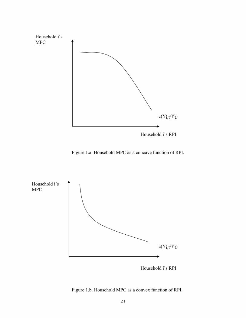
Figures 1.a and 1.b show household MPC as a function of RPI. In Figure 1.a the

MPC is drawn as a quasi-concave function so that the MPC falls rapidly for some range

as RPI rises. In Figure 1.b the MPC is drawn as a convex function so that the decline in

MPC tapers off as RPI rises.

7

The shape of the MPC function has important consequences with regard to the

impact of income distribution on aggregate consumption. This can be seen readily by

considering the case of an economy with two types of household, one with low income

and the other with high income. In this case the economy-wide average MPC is the

weighted average of the individual household MPCs. In terms of Figures 1.a and 1.b it is

a point along a chord connecting the individual household MPCs. The distance between

the economy-wide weighted average MPC and the individual household MPC is

inversely proportional to the weight given to each household type.

Now, consider an increase in income inequality for the case of a strictly concave

MPC. This increases the relative income of the high-income household, decreases the

relative income of the low-income household, and widens the gap between the MPCs of

the households. As a result the chord joining the two households shifts toward the origin,

and the average MPC falls. This will tend to lower aggregate consumption, so that

widened income inequality is bad for consumption. Conversely, if the MPC is a convex

function, widening income inequality will tend to raise the average MPC so that the net

impact of the redistribution is mitigated.

The economic logic for these impacts is easily understood in terms of absolute

and relative income effects. The redistribution of income lowers the absolute income of

low-income households and increases that of high-income households. Since low-income

households have a higher MPC, this lowers aggregate consumption spending. However,

the shift also lowers the relative income of low-income households, which increases their

MPC and positively impacts aggregate consumption. Conversely, it raises the relative

income of high-income households, which lowers their MPC and lowers aggregate

8

spending. If the “keeping up with he Joneses” effect (the relative income effect) is very

strong among low-income households (i.e. the MPC is convex), then it will reduce the

negative effects on consumption from redistributing income from low- to high-income

households. Indeed, it is theoretically possible that the net effect could even be positive if

the net relative income effect dominates the net absolute income effect.

The above microeconomic description of household consumption behavior can be

incorporated in a model of aggregate consumption as follows. There are two types of

household, and their consumption spending is described by:

(3) Ci,t = c(Yi,t/Yt)Yi,t i = 1,2

Relative income is given by (4) Y1,t = aY2,t 0 < a < 1

where a = relative income parameter. Since a < 1, this implies type 1 households are low

income households. The distribution of aggregate income across household types is given

by:

(5) Yt = qY1,t + [1 - q]Y2,t 0 < q < 1

= qaY2,t + [1 - q]Y2,t

where q = household composition parameter, and Yt = exogenous average income.

Aggregate per capita consumption is a weighted average of household consumption

and given by:

(6) Ct = qc(Y1,t/Yt)Y1,t + [1-q] c(Y2,t/Yt)Y2,t

Substitution of equations (3), (4) and (5) into equation (6) then yields the following

reduced form expression for the aggregate consumption function.

(7) Ct = qc(a/[1+qa-q])aYt/[1+qa-q] + [1-q] c(1/[1+qa-q])Yt/[1+qa-q]

9

Disequilibrium lag and habit ratchet effects, which are the second part of

Duesenberry’s theory can be readily incorporated into the model by adding the following

lagged adjustment mechanism:

(8) Ci,t – Ci,t-1 = k1[C*i,t - Ci,t-1] + k2D[C*

i,t - Ci,t-1]

where C = actual consumption, C* = desired consumption = c(Yi,t/Yt)Yi,t, k1 and k2 =

adjustment coefficients, and D = indicator variable that 0 if dY > 0 and 1 if dY < 0. The

theoretical rational for such lagged adjustment effects is that there are psychic costs to

adjusting consumption, and these psychic costs are asymmetric and larger for downward

adjustments.3

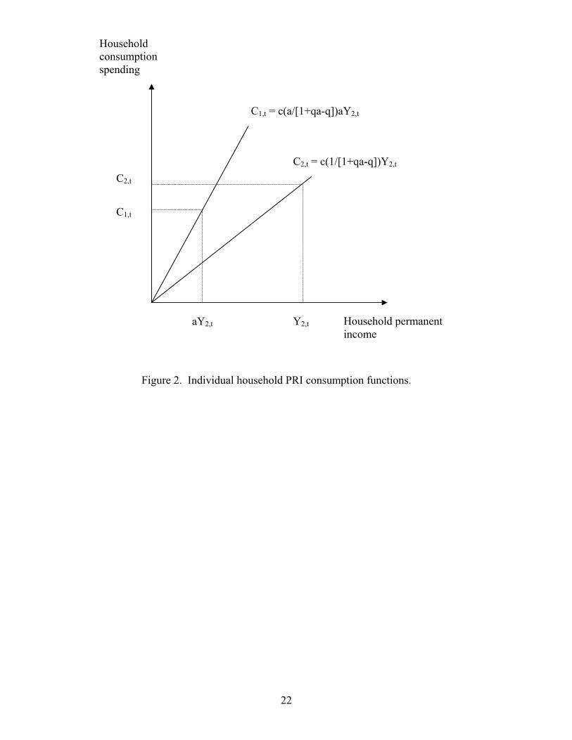
Figure 2 shows the individual household PRI consumption functions described by

equation (3) in the model. The individual household’s consumption function is a ray from

the origin similar to that of permanent income consumption theory. However, the

consumption function of the household with higher relative income lies strictly below

that of the household with lower income.

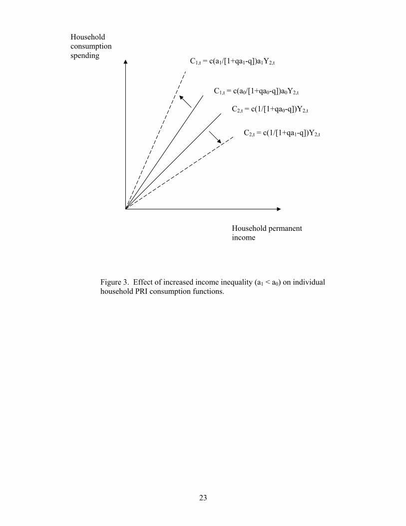
Figure 3 shows the effect of worsened distribution of income (a1 < a0) on the

individual household consumption functions. The low-income household’s consumption

function rotates counter-clockwise reflecting the impact of lower RPI, while the high-

income household’s consumption function rotates clockwise.

IV Analytics of aggregate consumption in an RPI model

There are two exercises to be considered. Exercise one is to derive the aggregate

consumption function and then examine its properties. Exercise two is to derive the cross-

section household consumption function and then examine its properties.

3 Dybvig (1995) provides a formalized utility theoretic model of ratcheting in which agents are subject to consumption addiction effects.

10

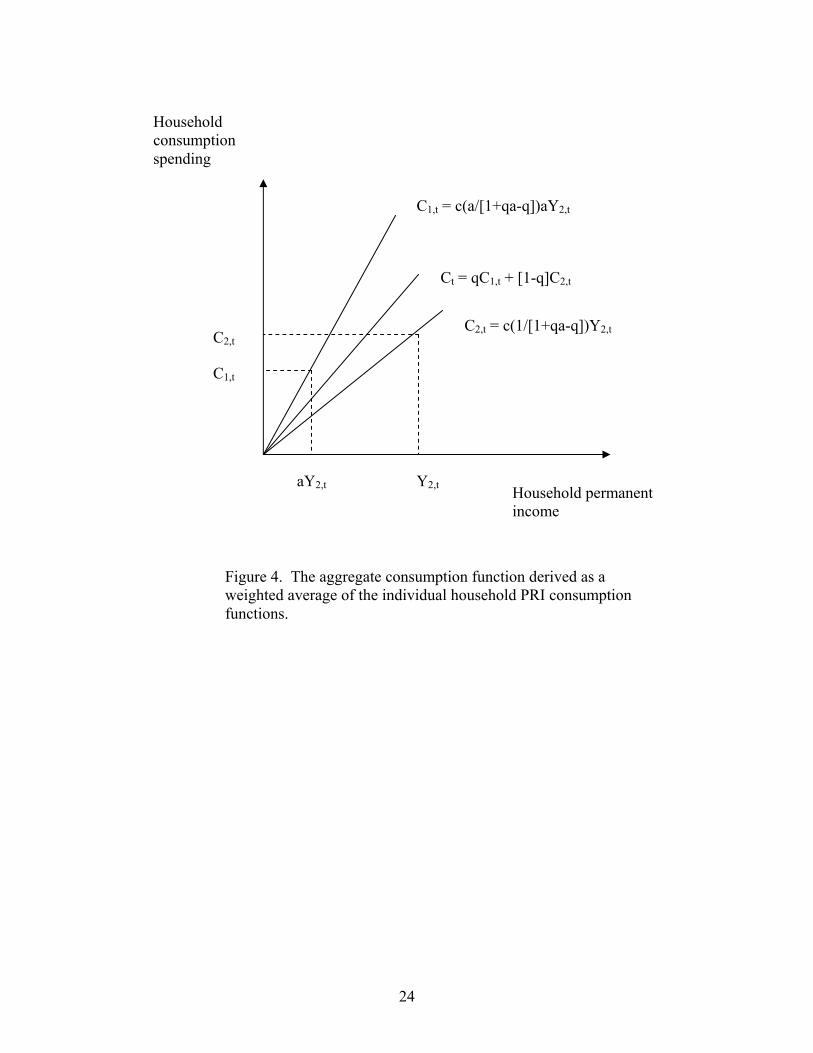
The aggregate per capita RPI consumption function is a weighted average of the

individual household RPI consumption functions and given by

(9) Ct = {qc(a/[1+qa-q]) + [1-q] c(1/[1+qa-q])}[1+a]Yt/[1+qa-q]

This aggregate consumption function is illustrated in Figure 4. It is a ray from the origin

lying between the individual household consumption functions. The aggregate

consumption function is a positive function of weighted average household income.

Assuming the distribution of income and the distribution of household types remains

unchanged, aggregate consumption will move along the aggregate consumption function

over time as income grows.

The aggregate MPC (i.e. slope of the aggregate consumption function) is given by

dCt/dYt = {qc(a/[1+qa-q]) + [1-q] c(1/[1+qa-q])}[1 + a]/[1+qa-q]

The aggregate MPC is therefore constant and independent of the level of income, a

feature that is consistent with Kuznets’ (1946) empirical findings. Inspection of the

expression for the MPC also shows that it is affected by the distribution of income (a) and

the composition of households (q), though the signs are theoretically ambiguous owing to

conflicting absolute and relative income effects

Exercise two concerns the derivation of the cross-section household consumption

function. This derivation is illustrated in Figure 5. At any moment in time households are

consuming according to their individual RPI consumption functions. The cross-section

consumption function corresponds to the linear function obtained by connecting the

household consumption - income points as shown in Figure 5. Simple linear algebra

yields a slope and intercept for the cross-section consumption function given by:

Slope = m = [C2,t – C1,t]/[Y2,t - Y1,t] = [c(1/[1+qa-q]) - c(a/[1+qa-q])a]/[1-a]

11

Intercept = b = [c(1/[1+qa-q])-c(a/[1+qa-q])]aY2,t/[1-a]

The slope and intercept terms are both functions of household income distribution (a) and

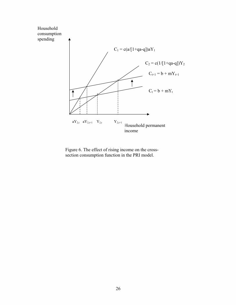
the composition of households types (q). The intercept is a positive function of the level

of income, and the cross-section consumption function therefore shifts up over time as

income rises. This shifting process is illustrated in Figure 6.

V Consistency with evidence on consumption behavior

The test of a theory is its consistency with known facts. The above RPI theory of

consumption is consistent with all the recognized stylized facts about consumption. First,

the theory generates a pattern of aggregate consumption that is consistent with Kuznets’

(1946) finding of a relatively constant long-run aggregate APC. Second, the theory

predicts that higher income households will have a higher average propensity to save and

a lower APC. This finding has been empirically documented by Carroll (2000), Dynan,

Skinner & Zeldes (1996), and Lillard and Karoly (1997).

Lastly, the theory predicts that the distribution of consumption will be more equal

than the distribution of income. This is because “keeping up with the Joneses” behavior

means that lower relative income households spend proportionately more of their income

than higher relative income households. Krueger and Perri (2002) confirm that the

distribution of consumption is indeed more equal than the distribution of income.

In sum, the proposed RPI theory is consistent with all of the major known stylized

facts concerning consumption spending. Contrastingly, other established theories of

consumption behavior – including Keynes’ aggregate consumption function, Modigliani

and Brumberg’s lifecycle model, and Friedman’s permanent income hypothesis – are not.

VI Interpreting the RPI Hypothesis in Terms of Utility Maximization

12

The RPI model of consumption behavior can also be incorporated in a utility

maximization framework that in turn shows how the RPI approach can also accommodate

Modigliani and Brumbergh’s (1954) lifecycle approach. This section presents a simple

description of such a framework.

The RPI consumption function developed earlier can be interpreted as the highly

“stylized” solution of a household lifetime utility maximization program given by:

∞ (10) Max Σ U(ci,t, ci,t/ct, wi,t/wt)/[1 + d]t U1 > 0, U2 > 0, U3 > 0 ci,t t = 0 Subject to (10.a) Σyi,t/[1 + rt]t + wi,0 = Σci,t/[1 + rt]t

(10.b) wi,t = wi,t-1 + yi,t - ci,t

where wi,t = household i wealth in period t, d = household rate of time preference, and rt

= real interest rate in period t. Average consumption (ct) and average wealth (wt)are taken

as given by households each period. Household i maximizes its discounted stream of

lifetime utility by choice of a consumption plan subject to a lifetime budget constraint

and a period wealth constraint. If income is certain and the interest rate and time

preference rate are zero, then households will consume a constant amount each period as

described earlier.

The particular representation given by equation (10) describes the household as

having an infinite horizon. Alternative specifications could have a finite horizon with a

bequest motive or with inter-generational altruism whereby the utility of future

generations is nested as an argument in the current generation’s utility function.

The key features of the utility function are the inclusion of relative consumption

and relative wealth as arguments. The inclusion of relative consumption captures

13

Duesenberry’s “keeping up with the Joneses” effect, which has been emphasized by

Frank (2005) in his work on positional goods. The inclusion of relative wealth is novel,

and represents the accumulation motive (Palley, 1993) that captures the desire for power.

The accumulation motive is an important concept that has not been addressed in the

mainstream microeconomic literature. It is important because it can explain why the rich

have a higher marginal propensity to save.

Consumption is a normal good so that the absolute level of consumption increases

with income. At the same time, if relative wealth is a luxury good (income elasticity > 1)

the accumulation of wealth will increase strongly with income. This configuration means

that consumption does not grow as fast as income, and the marginal propensity to save

increases as households get relatively richer because the accumulation motive kicks in

with greater force.

In principle, given the above specification of the individual household utility

maximization program it is then possible to derive an aggregate consumption function

that has demographic dimensions as is done in the standard life-cycle model. Thus,

household consumption decisions can vary with household age, and the aggregate

consumption function will then also depend on the age distribution of households (Fair

and Dominguez, 1991). Debt and liquidity constraints can also be incorporated by

appropriately modifying the wealth constraint given by equation (10.b).

Such a utility maximizing construction of the RPI model adds additional

psychological richness to the theory of consumption. That utility is inter-dependent

should not be a surprise. Love, altruism, envy, jealousy, power, and status are all sources

14

of utility, and all have elements of inter-dependence. The above specification

incorporates both status and power concerns in the utility function.

The inclusion of relative consumption and wealth as arguments of the utility

function helps explain why publicly reported happiness levels do not appear to have risen

much over the last three decades despite large increases in household income

(Blanchflower and Oswald, 2000; Layard, 2005) If all household incomes rise together,

the only utility gain comes from increased absolute income. If both absolute income and

income inequality are rising, the public could on average report diminished happiness if

the relative income effect dominates the absolute income effect.

VI Some further policy implications

The proposed theory of consumption behavior has both macroeconomic and

microeconomic policy implications. With regard to macroeconomics, the fact that lower

income households have a higher MPC and lower MPS lends the model a traditional

Keynesian tilt. Thus, redistributing income to lower income households is likely to have a

net positive effect on aggregate demand owing to “keeping up with the Joneses”

behavior. Similarly, tax cuts aimed at the bottom of the income distribution are likely to

be more expansionary than tax cuts aimed at the top. However, to the extent that

consumption behavior is still predicated on assessments of relative permanent income,

the impact of tax cuts will be greater the more that they are perceived as permanent or the

more liquidity constrained are households.

At the microeconomic level, the model suggests policy that constrains emulation

behaviors can improve social welfare. In effect, households are partially engaged in a

form of consumption “arms race”. The rich try to increase relative consumption while

15

lower income households try to keep up with the Joneses. That suggests a place for

policies that limit the arms race. Consumption taxes on luxury goods are one possible

tool, being progressive in incidence and discouraging conspicuous consumption by the

rich that imposes a negative externality on lower income households.

Rather than focusing directly on spending behavior, policy might be focused on

income earning behavior since it is income that fuels the arms race. The attempt to earn

income to pay for consumption may cause households to overwork. In effect, the

consumption arms race may get shifted back into labor markets and the workplace. That

in turn can drive down wages because of increased labor supply and result in excessive

hours per worker. This suggests there may be a place for labor market “ceilings”, such as

the forty-hour week, to limit spillovers from the consumption arms race into the labor

market. Economists often focus on the need for labor market “floors” to prevent

exploitation, but problems associated with emulative behavior suggest there is also a

place for labor market ceilings.

VII Why was Duesenberry’s theory discarded?

Duesenberry’s relative consumption approach is socially and psychologically

rich, and seems highly compelling. Why then was Duesenberry’s theory discarded by the

economics profession after the 1950s? One possible reason is that – unlike Keynes,

Modigliani and Brumberg, and Friedman – the relative income approach never developed

a tractable diagrammatic framework suitable for classrooms, and with clear differentiated

predictions and policy implications.4 This may have cost relative income theory dearly

4 In comments made at a conference at which this paper was presented Robert Solow suggested that Duesenberry’s model may have been bypassed for the most trite of reasons, namely that it failed to generate interesting exam questions for students.

16

given the economics profession’s penchant for mathematical and diagrammatic

treatments.

A second possible reason for neglect of Duesenberry’s theory may have been its

failure to frontally address the two major empirical controversies surrounding

consumption. These controversies concern (i) the long run constancy of the aggregate

average propensity to consume and (ii) the flatter slope of the short run consumption

function relative to the long run consumption function with regard to income.

A third reason is that properly representing Duesenberry’s theory in a utility

maximizing framework requires adding arguments to the utility function. That is

something the economics profession has systematically resisted on grounds that this

constitutes “ad hoc” theory – though that itself seems a rather hollow objection because

something has to be placed in the utility function and exclusion is equally ad hoc.5

A fourth reason is that Duesenberry’s ideas were resisted because utility inter-

dependence is highly destructive of neo-classical welfare economics. In effect, it hollows

out the concept of Pareto optimality, which is already fairly narrow. If relative

consumption and wealth matter for individual’s utility, then it is very hard to make all

better off since raising the income of one while leaving the incomes of others unchanged

is not Pareto improving.

Finally, Duesenberry’s ideas may have been by-passed because of the chilling

effects of the politics of the Cold War. Communist societies emphasized egalitarian

concerns, and Duesenberry’s ideas can easily lead in this direction because of their

emphasis on relative income and relative consumption. At a time when the United States

5 There is now growing realization that modifying the utility function is essential for explaining economic behaviors associated with such phenomena as effort, fairness, and identity.

17

was engaged in global geo-political struggle with the Soviet Union, the tendency of

Duesenberry’s arguments to legitimize egalitarian concerns may have provoked

resistance to incorporating relative well-being arguments in neo-classical economics.

After all, economists are also members of society, and they too are impacted by the social

and political controversies of the moment, just as are ordinary people.

18

References Ackley, G., Macroeconomic Theory, New York: Macmillan, 1960. Alpizar, F., Carlsoson, F., and O. Johansson-Stenman, “ How Much Do We Care about Absolute Versus Relative Income and Consumption?” Journal of Economic Behavior and Organization, 56 (2005), 405 – 21. Bagwell, L.S., and B.D.Bernheim, “Veblen Effects in a Theory of Conspicuos Consumption,” American Economic Review, 86 No. 3 (June 1986), 349 – 73. Blanchflower, D.G. and A. Oswald, “Well-being Over Time in Britain and the U.S.A.,” NBER Working Paper No. 7487, January 2000. Carroll, C.D., “Why do the Rich Save so Much?” in Does Atlas Shrug? The Economic Consequences of Taxing the Rich, ed. by Joel Slemrod, forthcoming, 2000. Dybvig, P.H.., “Duesenberry’s Ratcheting of Consumption: Optimal Dynamic Consumption and Investment Given Intolerance for Any Decline in Standard of Living,” The Review of Economic Studies, 62 No.2 (April 1995), 287 – 313. Duesenberry, J.S., “Income - Consumption Relations and Their Implications,” in Lloyd Metzler et al., Income, Employment and Public Policy, New York: W.W.Norton & Company, Inc., 1948. ---------------------, Income, Saving and the Theory of Consumption Behavior, Cambridge, Mass.: Harvard University Press, 1949. Dynan, K.E., Skinner, J., and Zeldes, S.P., “Do the Rich Save More?” Manuscript, Borad of Governors of the Federal Reserve System, 1996. Fair, R.C. and K.M.Dominguez, “Effects of Changing U.S. Age Distribution on Macroeconomic Equations,” American Economic Review, 81(5) December 1991, 1276-1294. Friedman, M., A Theory of the Consumption Function, Princeton: Princeton University Press, 1956. Frank, Robert H., “Positional Externalities Cause Large and Preventable Welfare Losses,” American Economic Review, 95, 2 (May 2005), 137 – 41. Keynes, J.M., The General Theory of Employment, Interest, and Money, London: Macmillan, 1936. Krueger, D., and F. Perri, “Does Income Inequality Lead to Consumption Inequality? Evidence and Theory,” NBER Working Paper No. 9202, September 2002.

19

Kuznets, S., National Product Since 1869 (assisted by L. Epstein and E. Zenks), New York: National Bureau of Economic Research, 1946. Layard, R. Happiness: Lessons from a New Science, London: Allen Lane: 2005. Lillard, L., and Karoly, L., “Income and Wealth Accumulation Over the Life Cycle,” Manuscript, Rand Corporation, 1997. Mason, R., “The Social Significance of Consumption: James Duesenberry’s Contribution to Consumer Theory,” Journal of Economic Issues, XXXIV (September 2000), 553 – 572. Modigliani, F. and R. Brumbergh, “Utility Analysis and the Consumption Function: An Interpretation of Cross-section Data,” in K. Kurihara (ed.), Post Keynesian Economics, London: George Allen and Unwin, 1954. Palley, T.I., "Under-Consumption and the Accumulation Motive," Review of Radical Political Economics, 25 (March 1993), 71-86. Patten, S., The Consumption of Wealth, Philadelphia: University of Pennsylvania Press, 1889. Schor, J.B., “In Defense of Consumer Critique: revisiting the Consumer Debates of the Twentieth Century,” The Annals of the American Academy of Political and Social Science, 611 (May 2007), 16 – 30.

20

Household i’s MPC

c(Yi,t/Yt)

Household i’s RPI

Figure 1.a. Household MPC as a concave function of RPI.

Household i’s MPC

c(Yi,t/Yt)

Household i’s RPI

21

Figure 1.b. Household MPC as a convex function of RPI.

Household consumption spending

C1,t = c(a/[1+qa-q])aY2,t

C2,t = c(1/[1+qa-q])Y2,t C2,t

C1,t

aY2,t Y2,t Household permanent income

Figure 2. Individual household PRI consumption functions.

22

Household consumption spending

C1,t = c(a1/[1+qa1-q])a1Y2,t

C1,t = c(a0/[1+qa0-q])a0Y2,t

C2,t = c(1/[1+qa0-q])Y2,t

C2,t = c(1/[1+qa1-q])Y2,t

Household permanent income

Figure 3. Effect of increased income inequality (a1 < a0) on individual household PRI consumption functions.

23

Household consumption spending

C1,t = c(a/[1+qa-q])aY2,t

Ct = qC1,t + [1-q]C2,t

C2,t = c(1/[1+qa-q])Y2,t C2,t

C1,t

aY2,t Y2,t Household permanent income

Figure 4. The aggregate consumption function derived as a weighted average of the individual household PRI consumption functions.

24

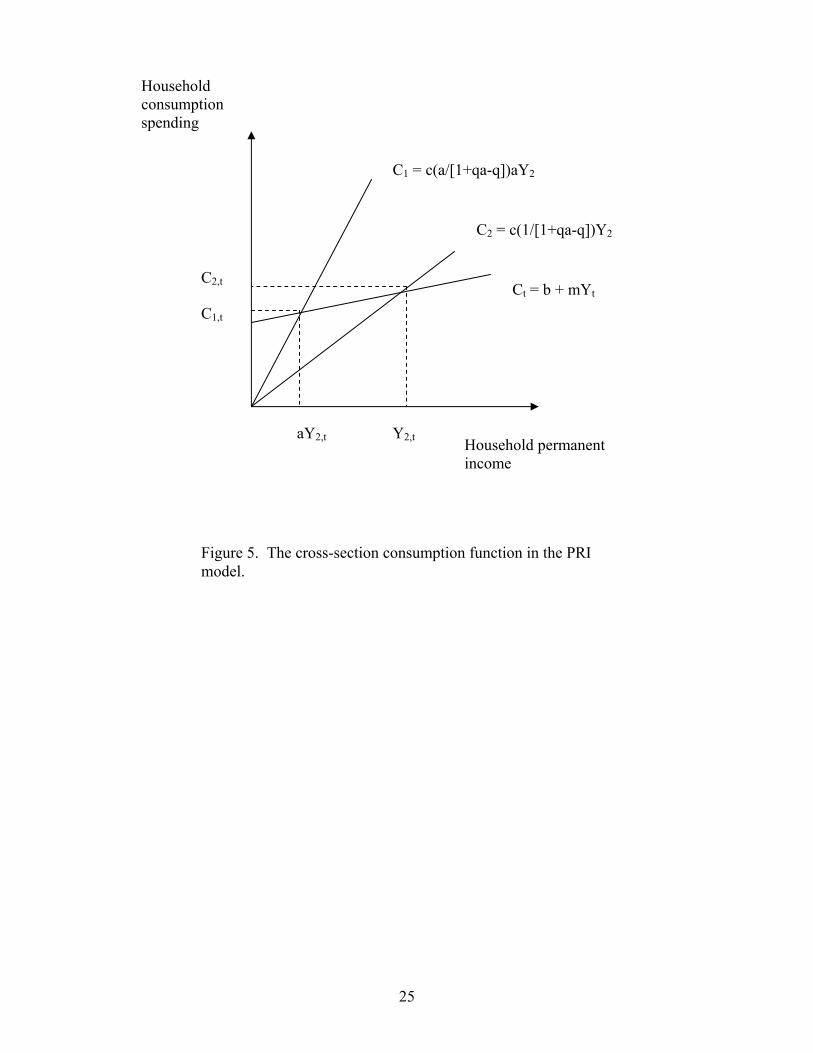
Household consumption spending

C1 = c(a/[1+qa-q])aY2

C2 = c(1/[1+qa-q])Y2

C1,t

C2,t Ct = b + mYt

aY2,t Y2,t Household permanent income

Figure 5. The cross-section consumption function in the PRI model.

25

26

Household consumption spending

C1 = c(a/[1+qa-q])aY1

Household permanent income

Ct = b + mYt

C2 = c(1/[1+qa-q])Y2

Ct+1 = b + mYt+1

Figure 6. The effect of rising income on the cross-section consumption function in the PRI model.

aY2,t aY2,t+1 Y2,t Y2,t+1