Embed Size (px)
Citation preview

ISSN 1518-3548 CGC 00.038.166/0001-05
Working Paper Series Brasília n. 261 Nov. 2011 p. 1-42

Working Paper Series Edited by Research Department (Depep) – E-mail: [email protected] Editor: Benjamin Miranda Tabak – E-mail: [email protected] Editorial Assistant: Jane Sofia Moita – E-mail: [email protected] Head of Research Department: Adriana Soares Sales – E-mail: [email protected] The Banco Central do Brasil Working Papers are all evaluated in double blind referee process. Reproduction is permitted only if source is stated as follows: Working Paper n. 261. Authorized by Carlos Hamilton Vasconcelos Araújo, Deputy Governor for Economic Policy. General Control of Publications Banco Central do Brasil
Secre/Comun/Cogiv
SBS – Quadra 3 – Bloco B – Edifício-Sede – 1º andar
Caixa Postal 8.670
70074-900 Brasília – DF – Brazil
Phones: +55 (61) 3414-3710 and 3414-3565
Fax: +55 (61) 3414-3626
E-mail: [email protected]
The views expressed in this work are those of the authors and do not necessarily reflect those of the Banco Central or its members. Although these Working Papers often represent preliminary work, citation of source is required when used or reproduced. As opiniões expressas neste trabalho são exclusivamente do(s) autor(es) e não refletem, necessariamente, a visão do Banco Central do Brasil. Ainda que este artigo represente trabalho preliminar, é requerida a citação da fonte, mesmo quando reproduzido parcialmente. Consumer Complaints and Public Enquiries Center Banco Central do Brasil
Secre/Surel/Diate
SBS – Quadra 3 – Bloco B – Edifício-Sede – 2º subsolo
70074-900 Brasília – DF – Brazil
Fax: +55 (61) 3414-2553
Internet: <http://www.bcb.gov.br/?english>
The relationship between banking market competitionand risk-taking: Do size and capitalization matter?
Benjamin M. Tabak∗ Dimas M. Fazio† Daniel O. Cajueiro‡
The Working Papers should not be reported as representing the viewsof the Banco Central do Brasil. The views expressed in the papers arethose of the author(s) and not necessarily reflect those of the BancoCentral do Brasil.
Abstract
This paper aims to study the effect of banking competition on LatinAmerican banks’ risk-taking and whether capitalization and size changes thisrelationship. We conclude that: (1) competition affects risk in a non-linearmanner: high/low (average) competition are related to more (less) stability;(2) bank’s size explains the advantage from competition, while capitalizationis only positive for larger banks in this case; (3) capital ratio explains theadvantage from lower competition. These results are of uttermost importancefor bank regulation, specially due to the recent turmoil in worldwide financialmarkets.
Key Words: bank competition, emerging market, financial stability,bank regulation
JEL Classification: D40, G21, G28
∗DEPEP, Banco Central do Brasil and Departament of Economics, Universidade Catolicade Brasılia†Departament of Economics, Universidade de Brasılia‡Departament of Economics, Universidade de Brasılia and National Institute of Science
and Technology for Complex Systems
3
1 Introduction
The analysis of banking competition has been of great concern in the lit-erature, specially due to its effects on the financial stability (Beck et al.,2006; Schaeck et al., 2009; Wagner, 2010). A competitive banking marketmay result in more benefits to the society as a whole, such as lower pricesand higher quality of financial products (Boyd and Nicolo, 2005), but on theother hand its influence on financial stability is not conclusive according tothe literature. There are two main rival theories on this matter. Some papersfind that competition, in fact, enhances bank risk-taking behavior, since itpressures banks to operate with a minimum capital “buffer” (Hellman et al.,2000; Allen and Gale, 2004). Others defend the contrary by stating thatcrises are less likely to happen in competitive banking systems (Beck et al.,2006; Boyd and Nicolo, 2005). Motivated by the process of deregulation andconsolidation that financial sectors around the world have been facing lately,specially on the developing world, our paper proposes to analyze whethercompetition has any effect on Latin American financial stability and if thisrelationship changes with other factors, such as size and capitalization. Ourinterest is to determine whether one of these theories better explain the caseof Latin American banks or even if they are both simultaneously valid.
The studies that support the concentration-stability (or competition-fragility) view state that banks may have a higher profit premium in collusivemarkets, creating a buffer from crises and therefore, reducing their incentivesto take risks (Hellman et al., 2000). In fact, in a competitive market, man-agers may be forced to take more risks on behalf of the shareholders, sincecompetition reduces the profits of managers and shareholders, as well (Kee-ley, 1990). Allen and Gale (2004) also affirm that this increased risk maybe due to a higher bank exposure to contagion in competitive markets. Anadverse shock can cause a bank to go bankrupt and, thus, it may triggera chain reaction where all banks that were exposed to the first bank alsogo bankrupt and so forth. Since under perfect competition these banks areprice-takers, and therefore small compared to the whole market, no bankwill have an incentive to provide liquidity to the troubled bank, causing thecontagion to spread. In addition, there is the matter of adverse selectionis worsened in a competitive market, i.e. in the presence of many banks inthe market (Broecker, 1990; Nakamura, 1993; Shaffer, 1998). The chanceof a poor quality borrower to apply for a loan at any bank is an increasingfunction of the number of banks, decreasing the quality of loan portfolio ofthe entire banking market.
A rival view, the “concentration-fragility” (or competition-stability), statesthat a more collusive banking market increases the financial fragility. Boyd
4
and Nicolo (2005) show that the higher interest rates charged by banks in aless competitive market may enhance the risk-taking behavior of borrowersand, therefore, increase the probability of a systemic risk1. The trade-off be-tween competition and risk ceases to exist in this analysis by assuming thatbanks are solving an optimal contracting problem. In other words, banks aresupposed to be agents in relation to their depositors, but they are also prin-cipal in relation to the borrowers. According to the authors, the literatureignores the bank-borrower relationship and for that reason it does not seecompetition as the social optimum.
Since competition cannot directly be measured, the literature has usedseveral different methods to estimate competitive levels of a specific sector.This paper, in particular, employs an innovative method to measure com-petition, known as the Boone indicator, which was introduced by the workof Boone (2008). This indicator measures the impact of efficiency on per-formance. The stronger this impact is, the higher the degree of competitiona bank is facing. A few works in fact have already used this measure forthe banking sector. For example, Schaeck and Cihak (2010) and Leuven-steijin et al. (2007) employs the Boone indicator for banks from the US andEurope. After that, in order to assess for whether the competition-stabilityor competition-fragility relationship holds for 10 Latin American countriesbetween 2001 and 2008, we regress the Boone indicator on the banks’ risktaking for these countries. This risk-taking measure is the “stability ineffi-ciency” from Fang et al. (2011), whose estimation approach is a StochasticFrontier Analysis (SFA).
Additionally, we are also interested to test how size and capitalizationchanges the relationship between competition and stability. In fact, as notedabove, the proponents of the concentration-stability view, state that largerbanks tend to operate better in collusive markets, even they have not pro-vided an empirical proof of this. Shaffer and DiSalvo (1994) demonstratethat the presence of large banks in relation to the market is not a sufficientcondition to reflect collusion 2. Thus, we would like to test if this assump-
1See Wagner (2010) for a extension of this analysis, where the author contradicts theconclusions of Boyd and Nicolo (2005). If one assumes that banks can choose between dif-ferent types of borrowers, competition can pressure these banks to finance riskier projectsso as to maintain their optimal risk-taking level.
2This matter has been thoroughly discussed in the literature. Claessens and Laeven(2004), for example, that find a positive relation between concentration and competition;Shaffer and DiSalvo (1994) that find a high degree of banking competition in a small Penn-sylvania county, even though the market structure was a duopoly; Maudos and Guevara(2007) that suggest that the effect of market concentration and competition on banks’ ef-ficiency is different. On the other hand, Bikker and Haaf (2002), Deltuvaite et al. (2007),Chan et al. (2007), Turk-Ariss (2009) regress competition indicators on market concen-
5
tion indeed holds by interacting the competition measure with a proxy ofsize. We also include an interaction between competition and equity ratio(capitalization) to test if a bank may be pressured to take more risks whenthey have an higher participation of sharholders’ capital in relation to theirassets given the competitive degree. There are two opposed effects in thiscase. Capital ratio can discipline banks due to the capital at risk effect,or decrease stability through a franchise value effect (Keeley, 1990; Hellmanet al., 2000). The overall effect is, then, ambiguous.
The recent world financial crisis has made bank regulators utterly inter-ested in determining how risk-taking depends on variables of market struc-ture, bank size and leverage (Basel Committee on Banking Supervision,2010). Through the implementation of the Basel III accord, they wouldlike to impose restrictions for banks to utilize a larger fraction of their owncapital in their operations. The objective is to reduce both the exposure tocontagion and the risk-taking behavior. In fact, the main concern of theseregulators regards the too big to fail (TBTF) banks. Because of their sys-temic importance, these banks are likely to incur in risks, believing that theauthorities will assist them if any problem should occur (basically, a moralhazard problem). Not only this creates instability in the banking market,but also TBTF banks are too costly to save (Demirguc-Kunt and Huizinga,2010b). The literature, therefore, must have a vanguard role in investigatingthis field so as to bring forth effective solutions for policy makers, specially onthe eve of the implementation of this accord. As already stated before, thisis our main motivation and, in the end, we intend to contribute relevantly tothis topic.
This paper is structured as follows: in Section 2, we describe our method-ology, defining the variables of interest and the regression approaches taken;in Section 3, we present and summarize the data sources; we demonstrateand discuss the empirical results in Section 4, and finally in Section 5 wemake our the final remarks regarding the outcome of this paper.
2 Methodology
2.1 The estimation of a competition measure: the Booneindicator
The fact that the competition level is not observable has resulted in manydifferent methods of measuring and estimating it. First, we may highlight the
tration and found a negative relationship, supporting the structure-conduct-performance(SCP) paradigm.
6
SCP paradigm, which have used concentration measures as proxy of compe-tition (e.g. Lloyd-Williams et al., 1994; Berger and Hannan, 1998). The ideaof this theory is that structure reflects conduct and, thus, market concentra-tion means collusion. Latter on, the New Economic Industrial Organization(NEIO) paradigm emerged with the idea of estimating parameters that re-flects the competition level of a market. The two most used are the modelsof Bresnahan (1982), and Panzar and Rosse (1987). The first calculates com-petition by estimating simultaneously the supply and demand function of agiven market, thus employing industry-aggregate data. Table 1 provides abrief review of the literature about the Bresnahan approach. The second iswidely utilized in studies about this matter, since it only requires easily avail-able data. This model use a reduced form revenue equation to construct theH-statistic, which is calculated as the sum of the elasticities of total revenuesin respect to factor input prices, i.e. it measures market power by the extentto which a change in factor input prices influences the equilibrium revenuesof a bank. Table 2 also presents a literature review on the papers that haveutilized this method.
Place Tables 1 and 2 About Here
In addition to these already popular measures, Boone (2008) has recentlydeveloped a new method of estimating competition. The Boone indicator(β), as it is called, considers that competition improves the performance ofefficient firms and weaken the performance of inefficient ones. The idea of thisindicator is clearly based on the efficiency structure hypothesis by Demsetz(1973). Thus, it measures the impact of efficiency on performance, in termsof profits and market shares. The stronger this effect is, the larger in absolutevalues β will be. The simplest equation to identify the Boone Indicator forbank i is defined as follows:
ln (MSki) = α + β ln (MCki), (1)
where MSki stands for the market share of bank i in the output k, MC isthe marginal cost, and β denotes the Boone Indicator. In this paper, weare going to focus on the analysis of competition in the loans market, sok = loans.
As an assumption of Boone (2008), competition means that the banks’products are close substitutes and/or entry costs are low. This itself is an ad-vantage of the his indicator over the concentration measures and some othercompetition proxies. Suppose, for example, that bank product substitution
7
increases. Then, efficient banks gain market share and, as the efficiencystructure hypothesis proposes, there is more competition in the market. Ifthese “efficient banks” are those which already have a dominant position inrelation to the others, the HHI would increase, instead of decreasing. Also,measures that imply that competition is inversely proportional to the mag-nitude of the price margin over marginal costs would not capture this effectas well. Efficient banks may charge higher prices because of their efficientlead, which can make them reduce marginal costs quicker than prices.
Among other advantages of the Boone indicator, we highlight the possi-bility of measuring competition for several specific product markets and alsodifferent categories of banks. This positive characteristic may have many in-teresting implications for future research on the competition issue. Not onlyit is possible to know which bank output is subject to more or less compet-itive pressures, but also we can compare different types of banks in termsof competition. As an example, Leuvensteijin et al. (2007) use the Booneindicator and, among other results, they find that commercial banks appearto face more competition than cooperative and saving banks, specially inGermany and the US.
On the other hand, there is also some disadvantages. For instance, be-cause of a efficiency improvement (i.e. a decrease in marginal costs), banksmay choose to decrease the price it charges in order to gain market shareor even to increase its profits and maintain the same share as before. We,therefore, have to suppose that banks pass at least part of its efficiency gainsto consumers. In addition, since we have to estimate this indicator, it isconstrained to the problem of idiosyncratic variation, i.e. uncertainty, as anyother estimated parameter.
Because one cannot observe marginal costs directly, Schaeck and Cihak(2010) approximate a firm’s marginal costs by the ratio of average variablecosts to total income, while Leuvensteijin et al. (2007) calculate the marginalcosts from a translog cost function for each country considered in their data.Our approach is similar to this last one, which is an improvement with respectto the former. Besides being more closely in line with the theory, the use ofa translog function offers the possibility of calculating the marginal costs ofany one of the outputs in the specification, such the loan market, whereastheir costs are also not directly available (Leuvensteijin et al., 2007). Weassume a translog cost function for bank i, and year t and estimate it foreach country in the sample separately. We then derive the marginal costsfrom its estimation and then we use this variable as the independent regressorof market share as in equation (1). Then, our cost translog specification hasthe following form:
8
ln
(C
w2
)it
= δ0 +∑j
δjlnyjit +1
2
∑j
∑k
δjklnyjitlnykit + β1ln
(w1
w2
)it
+1
2β11ln
(w1
w2
)it
ln
(w1
w2
)it
+∑j
θjlnyjitln
(w1
w2
)it
+ Dummiest + εit, (2)
where C stands for the bank’s total cost; y represents four outputs: totalloans, total deposits, other earning assets, and non-interest income, this lastbeing a measure of bank non-traditional activity3; w consists in two inputprices: interest expenses to total deposits (price of funds), non-interest ex-penses to total assets (price of capital)4. The objective of normalizing thedependent variable and one input price (w1) by another input price (w2) isto ensure linear homogeneity.
Thus, we can obtain the marginal costs of loans (l) if we take the firstderivative of the dependent variable in equation 2 in relation to the output
yilt (loans): MCilt = ∂(Cit/w2)∂yilt
=(Cit/w2
yilt
)∂(lnCit/w2)∂ln yilt
, or more detailed:
MCilt =
(Cit/w2
yilt
)(δj=l + 2γllh ln yilt +
∑k=1,...,K;k 6=l
γlkh ln yikt) (3)
Having calculated the marginal costs for loans, we can proceed to esti-mating the Boone indicator as in equation (1), but with small changes. Inthis study, we will calculate the Boone Indicator in two different specifica-tions. First, we evaluate the competitive conditions for each Latin Americanbanking market in the whole period; second, we assess for the changes incompetition through the years in these same countries. The estimation ofthe following equation for each country separately gives us the competitiveconditions in the loans market for the full sample period:
ln (MSilt) = α + β ln (MCilt) +Dummiest + eilt. (4)
3There is a growing acceptance in the incorporation of variables of bank non-traditionalactivities (such as off-balance sheet and non-interest income) in the banking analysis(Lozano-Vivas and Pasiouras, 2010). Ignoring these measures can be misleading, sinceit does not take into account the bank’s balance sheet as a whole. Due to a high num-ber of missing values on Latin American banks’ off-balance sheet, we only employ thenon-interest income as a non-traditional output.
4Total assets is employed instead of fixed assets due to several missing data of thelatter.
9
The equation above represents the relationship between individual marketcosts (MCilt) and market shares (MSilt) in the loans market of bank i at timet. We also add time dummies to control for timely evolution of the marketshare within a country. We expect that banks with low marginal costs gainmarket share, i.e. β < 0. Competition tends to increase this effect, sincemore efficient banks outperform less efficient ones. The more negative is β,the higher is the competition level in a banking market. However, positivevalues for β are also possible as we can see in Leuvensteijin et al. (2007).This means that the more marginal costs a bank has, the more market shareit will earn. We can think of two reasons to explain this phenomena: (i) themarket has an extreme level of collusion or (ii) the banks are competing onquality. This last reason may reflect strong collusion, as well. Banks mayincrease their costs in order to capture additional demand by the qualitychannel as the market as a whole grows, which is a clear obstruction of theentry of competitors in this same market (Dick, 2007).
However, it is not enough to observe how strong competition for theperiod as a whole. We are also interested to observe the time evolution ofthe degree of competition. In order to assess this time development, weconsider the following equation, where we interact the Boone Indicator withtime dummies, making it time dependent:
ln (MSilt) = α +∑
t=2001,...,2008
βt Dummiest ln (MCilT ) +DummiesT + eilt.
(5)The estimation of the Boone indicator for each year t is a result of this
specification. We can, therefore, analyze how competition has changed overtime by considering the intensity banks with low marginal costs in loans gainsmarket share in this market by year.
As in Leuvensteijin et al. (2007) and Schaeck and Cihak (2010), we arealso aware of a possible endogeneity problem in the estimation of equations(4) and (5). Both papers point out that the determination of performanceand cost are determined simultaneously. Our approach is first to test whetherendogeneity is indeed present in our specifications. This tests consists in thedifference of two Sargan-Hansen statistics: one for the equation where wetreat MC as endogenous, and one for the equation where we treat MCas as exogenous. Under conditional homoskedasticity, this endogeneity teststatistic is numerically equal to a Hausman test statistic (see Hayashi, 2000,for more information). Consequently, if we confirm this problem, we utilizea two-step GMM estimator where we use one lag of MCilt as instrument.Otherwise we use a fixed-effects OLS method, more specifically the within
10
estimator, to regress the models. In both cases we perform the kernel-basedheteroscedasticity and autocorrelation consistent (HAC) variance estimationby Newey and West (1987), in order to control for both of these problems.
2.2 Evaluating the impact of competition on risk-taking
In this subsection, we present the empirical analysis of the relationship be-tween competition and risk-taking. For this purpose, we employ a measurethat reflects banks’ risk-taking behavior, the Z-score. Many other studiesevaluating bank risk-taking behavior also use this measure, which confirmsits acceptance in the literature (Mercieca et al., 2007; Laeven and Levine,2009; Houston et al., 2010; Demirguc-Kunt and Huizinga, 2010a). The Z-score measures the number of ROA standard deviations that a bank’s ROAplus its leverage have to decrease in order for the bank to become insolvent(or Z − score = (ROA+Capital Ratio)/σROA). In other words, the Z-scoreis inversely proportional to the bank’s probability of default.
This measure has been often employed in cross-section OLS models, whereone can calculate the mean and standard deviation of ROA for the wholeperiod. We, however, propose to calculate this measure for each three years(present year and the two precedents) so as to maintain the Z-score as anpanel variable. Instead of eliminating the time dimension of the analysis,this approach only reduces the time period we consider by two-years.
In addition, we follow the model that Fang et al. (2011) introduce, toestimate the impact of competition, size and capital on bank’s risk tak-ing. This method consists in estimating a stochastic frontier (Aigner et al.,1977; Meeusen and van den Broeck, 1977) with the Z-score as the dependentvariable of the translog specification, so as to provide a measure of bank’s“stability inefficiency”. The main idea of these authors is that the Z-scoredoes not necessarily reflect the potential stability each bank can achieve.One has also to consider the deviation from banks’ current stability and themaximum stability given the economic and regulatory conditions, which theydenominate as the “stability efficiency” analysis. At the same time, we em-ploy the inefficiency explanatory variables in the specification through themethod of Battese and Coelli (1995). Thus, we use the maximum likelihoodto estimate the Z-score translog specification and the inefficiency correlatessimultaneously.
The equation we consider for estimating this frontier is very similar ofequation (2), but instead of C (costs) we employ the Z-score and the errorterm εit equals νit − υit. The first term (νit) captures the random distur-bances, assumed to be normally distributed, and representing measurement
11
errors and other uncontrollable factors, i.e., νitiid∼ N(0, σ2
ν). The second (υit)captures technical and allocative inefficiency, both under managerial control,and it is assumed to be half-normally distributed, i.e., υit ∼ N+(µit, σ
2υ). The
degree of “stability efficiency”, in this case, represents how close a bank isto the maximum Z-score, i.e. the stochastic frontier. The model to estimatethe frontier is as follows:
ln
(Z-score
w2
)it
= δ0 +∑j
δjlnyjit +1
2
∑j
∑k
δjklnyjitlnykit + β1ln
(w1
w2
)it
+1
2β11ln
(w1
w2
)it
ln
(w1
w2
)it
+∑j
θjlnyjitln
(w1
w2
)it
+ lnNPI
+ α1T + α2T2 + Macroeconomic Variables + νit − υit, (6)
where the output and input variables are the same from equation (2). Weemploy country environment variables in order to control for cross-countryheterogeneity of banking markets. The use of macroeconomic variables in thetranslog functions has been considered very important by the literature inthe correct estimation of cross-country efficiency scores (Dietsch and Lozano-Vivas, 2000; Fries and Taci, 2005). These variables reflect specific character-istics, such as geography, economic condition and financial dynamism, andwe detail them next. First, we employ the density of population, measured bythe ratio of inhabitants per square kilometers, because we believe that banksoperating in a region with a high density of population might have lowerexpenses. We use the density of demand, i.e. the ratio of total deposits tosquare kilometers, so as control for the possible higher bank expenses whenthe density of demand is low. We employ the GDP per capita to assess forthe general development of the economy. The purpose of also employing theratio of equity to assets is to control for the regulatory conditions. In addi-tion, we use the ratio of loans to deposits that consists on the rate in whichdeposits are converted into loans, i.e. the size of intermediation. Finally, wealso use the real GDP growth, as a proxy of economic dynamics.
There is, however, a problem in applying the natural logarithm of the Z-score in equation (6), since this variable can take negative values as well. Inorder to solve this problem we follow Bos and Koetter (2009) who employs anadditional independent variable - the Negative Performance Indicator (NPI)- that takes the value of 1 when Z-score ≥ 0 and it is equal to the absolutevalue of Z-score, when Z-score < 0. We also change the dependent variableto take the value of 1, when it is negative.
As we have already stated, parallel to the estimation of this stabilityfrontier we also introduce the inefficiency correlates in the model. In other
12
words, we define the mean value of the inefficiency term µit for the Z-scorefunction as follows:
µit = δ0 +∑n
δnitznit (7)
where z is a vector of n bank-specific variables that explains efficiency ofbank i at time t. In our case, this vector of variables comprises the followingvariables: (1) the opposite of Boone indicator (i.e. −βt) that we estimatefrom equation (5) and its square value, as well; (2) the equity to assets ratio(Capital Ratio), as a measure of capitalization; (3) liquid assets to totalassets ratio (Liquidity), as a measure of liquidity; (4) the natural logarithmof assets (SIZE); (5) and the loan loss reserves to gross loans (LLR, in%) to control for bank’s loan portfolio risk. Finally, we also add ownershipdummies to assess for differences of stability inefficiency across different bankownership type.
The idea of employing the opposite of the Boone indicator is to makeit directly proportional to competition. Moreover, we also add a quadraticterm of this measure to capture a possible non-linearity of the competition-risk relationship. Although this non-linear analysis can have a crucial im-plication to the financial stability debate, it has been largely overlookedby the literature. Finally, with the purpose of making the results clearer,and also robust, we also add specifications in which we employ competitiondummies instead of the Boone indicator. These dummies are for High (≥Boone+0.5σBoone), Average (< Boone+0.5σBoone and > Boone−0.5σBoone)and Low (≤ Boone − 0.5σBoone) competition. The division of competitioninto three different categories has the purpose of identifying possible non-linearities in the model, as well.
As an additional test, we are also interest to analyze whether the competition-risk relationship changes among different bank size and capitalization. Wetest if larger banks outperform others in collusive markets due to higher prof-its, and/or if the magnitude of shareholders’ capital can in fact force banksto take on more risks. In this regard, Carletti (2010) affirms that fundingand regulation have the same importance as market structure for explaininghow the recent crisis has affected different banking sectors. To achieve thisresult, we add the following specifications to equation (6) by interacting theBoone indicator and its square term with: (i) SIZE; (ii) Capital Ratio; (iii)both Capital Ratio and SIZE. We also estimate these specifications againinteracting all three dummies of competition with SIZE and Capital Ratio.
13
3 Data
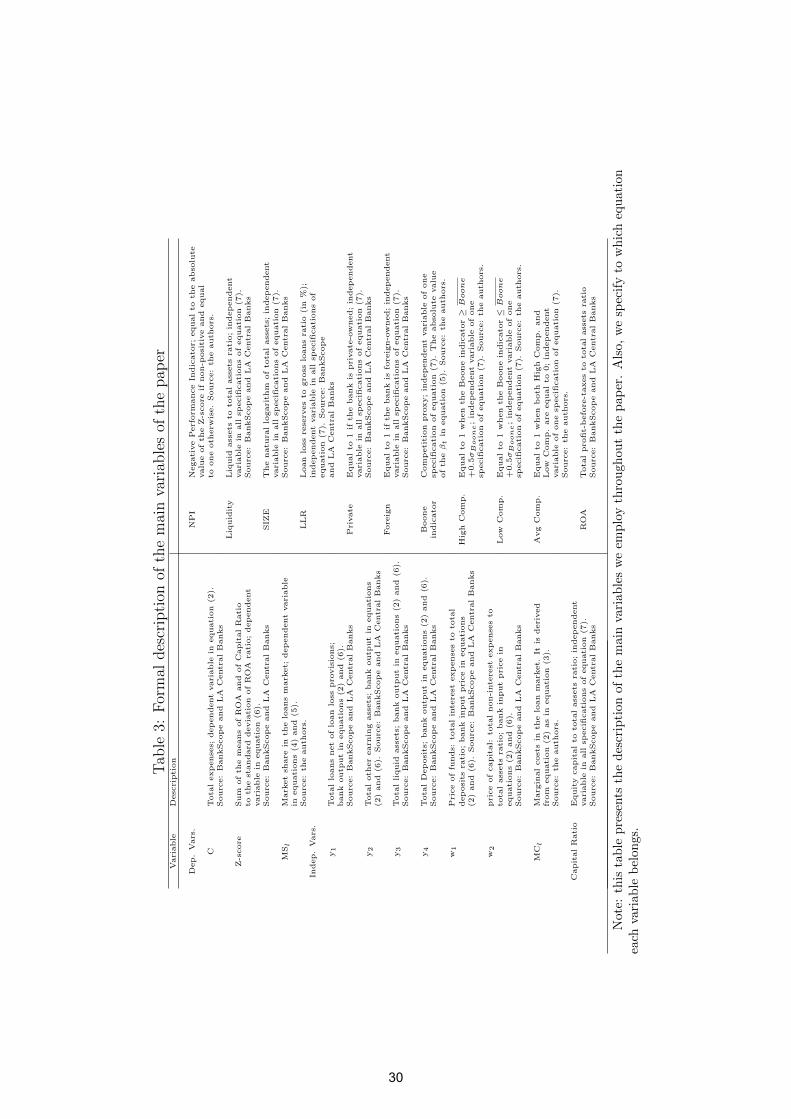
Initially, our data consisted in the population of four bank specializations -commercial, cooperative, real-state and specialized government institutions- that had been operating in 10 Latin American countries from 2001 to2008. We have taken the relevant data from from the BankScope, a finan-cial database distributed by BVD-IBCA and converted to US dollars, whichguarantees accounting uniformity between different countries. We also checkcarefully these data in the respective countries’ central banks. After exclud-ing banks/periods with missing, negative or zero values for inputs and out-puts and other relevant data, our resulting sample for estimating the Booneindicator is an unbalanced panel data of 376 banks, totalizing 2243 observa-tions. Additionally, since we have used two time lags in order to calculate theZ-score our database to estimate the risk-taking correlates reduced to 1491observations from 2003 to 2008. Table 3 shows the names and descriptionsof the variables we use in the models of last section.
Place Table 3 About Here
First of all, Table 4 shows the summary statistics of the bank-level vari-ables used in the translog specifications by country. From this Table, onemay identify that the banks from some of the main economies in the region,such as Mexico, Chile and Brazil, have on average the largest loan and de-posit portfolios. On the other hand, the smallest banking systems in termsof loans and deposits, for example are those from Costa Rica and DominicanRepublic. Nevertheless, the size of the banking market does not seem to re-flect overall stability. In terms of the Z-score, the banking markets of CostaRica, Panama and Chile are the most stable, while those of Argentina andBrazil are the least stable.
Place Table 4 About Here
Second, the summary of the variables we use in the risk-taking modelis available in Table 5. This Table also includes the percentiles to betterunderstand how distributed are these variables. As one can observe from theZ-score and LLR variables, our data encompasses banks that are practicallybankrupt (low Z-score and high LLR), and extremely stable banks (high Z-score and low LLR). Furthermore, the bank’s size variable (SIZE) ranges
14
from 8.941 (bank assets equal to U$ 7.639 millions) to 19.36 (bank assetsequal to U$ 255.823 billions) that reflects a widely dispersed distribution ofthis variable.
Place Table 5 About Here
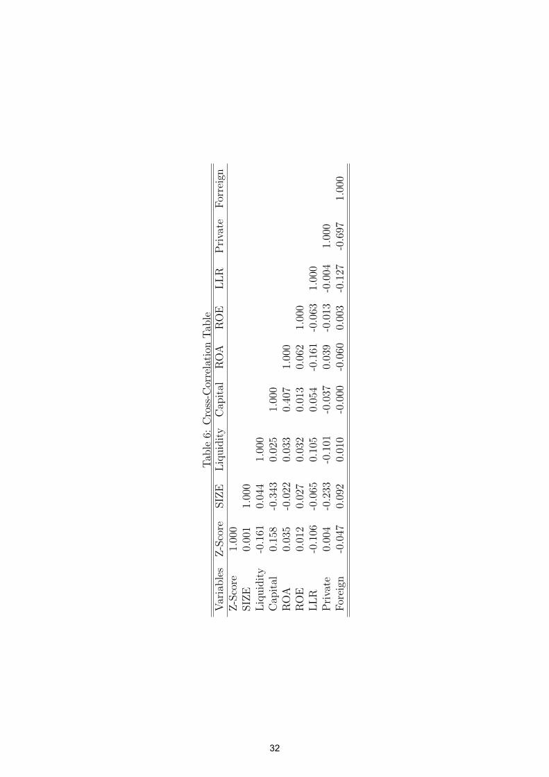
Additionally, in Table 6, we show the cross-correlation between our mainindependent variables of the model. An interesting thing to note is that sizeappear to be negatively correlated with the capital ratio, which means thatlarge banks have a higher propensity to use capital from other entities, i.e.to acquire liabilities. This fact will be important in the following sections,since our goal is to determine whether size and capital ratio changes therelation between competition and risk. Greater capital ratio also seems toreflect higher stability, because of the positive correlations with Z-score andROA. We will confirm this last result latter.
Place Table 6 About Here
Finally, Table 7 presents the means and standard deviations of the country-environment variables that we employ in the Z-score translog specification.They consist in economic and financial sector development indicators in orderto access for cross-country differences in economic and financial conditions.These macroeconomic data were taken from the IMF’s World Economic Out-look, World Bank’s database, and BankScope5. In fact, in Latin America,there are some essential economic differences between countries. While thereare some with a dynamic economy and satisfactory social conditions, othercountries are more vulnerable and present poor social indicators. Thesevariables may have direct influence on the profitability and stability of thecorresponding banking systems.
Place Table 7 About Here
5Bank’s deposits, loans, assets and equity by country have been aggregated using theoriginal database from the central banks to proxy for total financial sector’s deposits,loans, assets and equity.
15
4 Empirical Results
4.1 Boone coefficient scores
In this section, we present the results from the Boone indicator estimation.In order to obtain the marginal costs, we estimate a translog cost functionsfor each country considered. Then, we regress these marginal costs on themarket share in the loans market. The coefficient of this last variable (β) isconsidered to be the Boone indicator. The more negative, this indicator is,the more competitive is a specific banking market.
Place Table 8 About Here
The results of the Boone indicator by country for the whole period con-sidered are presented in Table 8. The endogeneity test has pointed out thatonly for Peru has marginal costs been considered endogenous (at 5% signif-icance level) in the estimation of equation (4). Thus, we employ a GMMestimator for this country and we use an OLS for all the others. The overallresult suggests that Latin American banks are operating in a less competi-tive market than in Europe and in the US, if we compare with the resultsfrom Leuvensteijin et al. (2007). However, we also acknowledge that this sortof comparison should be made carefully, since the estimation of the Booneindicator, depends on how it was modeled. For example, Schaeck and Cihak(2010) have employed in the Boone estimation ROA instead of market shareas the dependent variable and average costs instead of marginal costs as theindependent variable. They found that the Boone indicator for the US andEurope was concentrated between 0 and -0.15. The model of Leuvensteijinet al. (2007), on the other hand, is closer to ours despite some differencesbeing apparent.
Another conclusion is that competition seems to be very heterogeneousacross Latin American countries, with Peru and Colombia being, respectively,the most competitive banking markets, and Chile and Costa Rica being themost collusive ones. In fact, the Boone indicator for Chile is not significantlydifferent from 0 (monopoly) at 10% significance level. Other large economiesof Latin America, like Brazil, Argentina, Mexico and Venezuela, show amoderate level of banking competition in this period. These results shed somelight in the development level of institutional framework of Latin Americancountries.
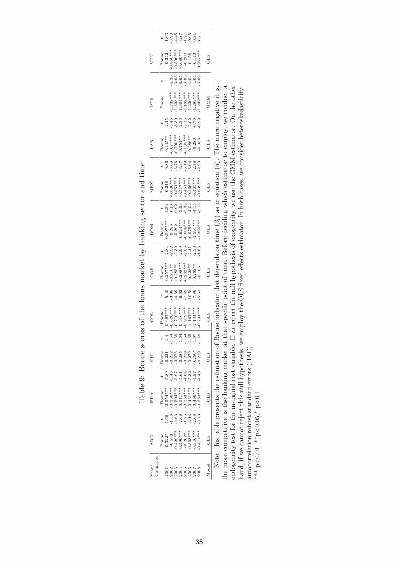
Place Table 9 About Here
16
We can also estimate the Boone indicator by year in order to consider thetime evolution of competition. Table 9 shows these Boone indicators for LatinAmerican countries. Through this analysis, we can observe that competitionhas evolved differently across Latin American countries. While in some coun-tries, competition has increased throughout the years (Argentina, Colombia,Dominican Republic, Mexico), in others competition has decreased (Brazil,Costa Rica, Panama, Venezuela). Competition has not changed significantlythrough time in Peru and Chile.
For some countries there are even years where the Boone indicator isnot statistically different from 0 (zero) or significantly positive. As we havealready stated before, positive values for this measure may mean perfectcollusion or competition in quality. The latter, however, may result in anincrease barriers to entry, i.e. more collusion as well. Consequently, perfectcollusion may be the case of Argentina in the years of 2001-2002 (peak of theeconomic crisis this country has faced); Chile for all the years except 2007;Costa Rica in 2008; Dominican Republic from 2001 to 2003; Mexico in 2001;Panama in 2007 and 2008; and Venezuela in 2001 and in 2005 to 2008.
4.2 Competition-Stability analysis
In this section, we present the results of our main model, whose objectiveis to estimate the relationship between competition and banks’ risk-takingbehavior, and how this competition changes due to the influence of capital-ization and size on risk-taking, as well. For example, Hellman et al. (2000)and Allen and Gale (2000) suggests that larger banks have a higher profitmargin in collusive markets, and this is why these banks are more stable inthese conditions. Competition can also pressure banks to take more risksdepending on size and capitalization of these banks.
Tables 10 to 13 show the estimations of equation (7), where we regress aseries of explanatory variables variables on the “stability inefficiency”. Neg-ative coefficients mean that the corresponding variables are inversely pro-portional to financial fragility, and thus they appear to increase stability.Positive coefficients, on the other hand, means that the variables are directlyproportional to fragility. In the first column of every Table we employ theBoone indicator as the proxy of competition. Since this indicator is inverselyproportional to competition (the more negative is this measure, the morecompetitive is a banking market), in reality we add the opposite of this indi-cator (Boone = −βt) so as to make it directly proportional to competition.In addition, the second to fourth columns of each Table employs dummiesthat represent high, average and low competition, respectively. Each tablehas one different specification as well in which we add interactions between
17
the competition proxies, size, and capitalization variables.
Place Table 10 About Here
We note from column [1] of Table 10 that the relationship between com-petition and risk taking appears to be
⋂-shaped. In other words, banks
operating under low and high competition levels are the less fragile ones,while banks under average competition are those with a more aggressiverisk-taking behavior. The negative and significant coefficients of high andlow competition dummies and the positive coefficient of average competitionin columns [2] to [4] confirm this result. Our findings accept (and at thesame time reject) the “concentration-fragility” and “concentration-stability”theories at the same time for Latin American banks. These results are similarto those of Berger et al. (2009) for 30 developed economies’ banking sectors.These authors state that finding evidence to support one of the theories doesnot necessarily excludes the other. However, we cannot yet affirm what arethe reasons of why banks are better of in both competitive and collusivebanking markets. We expect that the other specifications will clarify thesereasons.
In what regards the other control variables, we may observe that loanloss reserves have a detrimental effect on stability. We have already expectedthis result, since the motive of adding this variable was to control for banks’exposure degree. The capital ratio has a negative and significant coefficient,which confirms the idea that banks are more cautions when the shareholdershave more capital at stake, i.e. the moral hazard hypothesis (see Berger andDeYoung, 1997). The coefficient of liquidity is positive and significant, andthus banks with more liquidity seem be farther from the stability frontier.We also conclude that private and foreign banks appear to be more inefficientin terms of stability in relation to public banks, as well.
Place Table 11 About Here
Table 11 shows the results on the specification in which we interact SIZEand competition variables, in which we want to know whether the impact ofsize varies with competition levels. In column [1], the interactions of SIZE andBoone and its square value show that the effect of SIZE on financial fragilityis⋂
shaped as a function of the Boone indicator. We must take the firstderivative of the first column in respect of SIZE to understand better how this
18
effect varies with the Boone indicator. This effect is as follows: ∂µ/∂SIZE =−9.10∗Boone2+7.75∗Boone−1.65, whose roots are 0.417 and 0.435. In fact,when we interact SIZE and the dummy of high competition in column [2], wefind from the sign of its coefficient that large banks appear to perform betterin less collusive markets. If the variable SIZE is larger than 10.13, i.e. with atleast U$25.2 million assets, the coefficient of the competition dummy becomesnegative 6. In column [3], the interaction between the average competitiondummy and SIZE is insignificant. Finally, column [4] shows that under a lowcompetition, banks are more stable for all values for SIZE, but decreasingin this last variable. At the same time, when Low = 1 the effect of SIZEbecomes slightly positive, but not significant in accordance with a Wald Test(p-value = 0.27). The other control variables have similar coefficients thanthose of the last Table.
The result above implies that we do not have reasons to accept the state-ment of the concentration-stability literature that larger banks in collusivemarkets are more stable, even though we cannot reject this theory per se (orat least half of it as discussed before), i.e. the fact that banks under lowcompetition are more stable. In fact, our findings suggest that larger banksare less risk-takers in a competitive environment. However, we cannot saythat under lower competitive levels, the effect of size is detrimental to overallstability due to the insignificant effects of columns [3] and [4]. There must beother reasons, therefore, for why low competition is also positive for banks’stability, such as the amount of shareholder’s capital, which we will analyzein Table 12.
Place Table 12 About Here
The⋂
-shaped effect on risk-taking as a function of competition also ap-pears to be the case of the Capital Ratio, as we can see by the first columnof Table 12. Column [4] supports these results, due to the negative coef-ficient of the interaction between the low competition dummy and capitalratio. The interaction coefficients in columns [2] and [3] are both insignifi-cant, suggesting that high and average competition levels do not change thenegative effect of capital ratio on stability inefficiency. Additionally, thesefindings also point out under low competition this negative impact of capitalratio is more pronounced. Therefore, collusive banking markets is positivefor overall bank stability, specially for those banks with a high capital ratio.
6A wald test shows that the effect of SIZE on inefficiency under high competitionbecomes significantly negative at approximately SIZE= 11.7.
19
This last statement gives support to Berger et al. (2009) when they affirmthat even if collusion leads to riskier loan portfolios (as in Boyd and Nicolo,2005), banks may increase their equity capital in order to protect maintaintheir overall stability. An effective regulamentary policy to reduce financialfragility would be the imposition of higher capital requirement that implieslower liabilities7.
Consequently, the results above show that capitalization explains why col-lusion reduces risk-taking in the Latin American banking market. Accordingto the definitions of Hellman et al. (2000), the capital-at-risk effect is greaterthan the franchise-value effect in the case of low competition in the LatinAmerican region. That is, there is no indication that capital ratio affectsfranchise values so as to force a bank to take risks. For example, Repullo(2004) affirms that this effect is insignificant if one assumes that the costsof higher capital requirements are fully transferred to the depositors of thatbank.
Although we have tested how size and capital interacts with competitionseparately, there is also the need to understand how is their jointly influenceon risk-taking. In other words, the question we pose is whether large banksbenefits the most from high (or low) capital ratios given the competitivelevel. Table 13 shows these results.
Place Table 13 About Here
Column [2] of this Table shows that, supposing the high competitiondummy equals to one, the interaction between SIZE and Capital Ratio be-comes more negative, and the coefficient of capital ratio alone becomes morepositive as well. The coefficients of “High Comp.” and SIZE, alone, areinsignificant, as well as its interaction. Therefore, the interpretation of theresults in the final column of this Table is as follows: for banks with assetslarger than U$ 222.2 million (SIZE = 12.31) and operating under high com-petition (i.e. High Comp. = 1) , the capital ratio appears to reduce stabilityinefficiency. Regarding column [3], when average competition is equal to one,we can conclude that the coefficient of the interaction of SIZE and capitalratio becomes closer to zero. Thus, there appears to be a positive effect of
7According to Carletti (2010), even within bank’s liabilities, the funding structure canhave an important role in explaining stability. In the recent financial crisis, banks aremore stable when they rely more on depository than on wholesale funding. In otherwords, banks that were more exposed to short-term borrowing, were deeply affected bythe financial crisis (Carletti, 2010)
20
Capital Ratio on the “stability inefficiency” for all banking sizes, but de-creasing in this last variable. Finally, all the interactions with the dummy oflow competition are insignificant in column [4].
5 Conclusion
This paper has the purpose of determining whether competition improves orreduces banking stability for 10 Latin American countries between the years2001 and 2008. Although there have been several articles concerning thisissue, the literature has not yet reached a clear consensus of whether compe-tition stimulates banks to take risks. Since competition cannot be calculateddirectly, we estimate, as a competition measure, the Boone indicator of theloans market, whose value shows how intense is the effect of more efficientbanks earning market share. Then, we regress this indicator on risk-taking soas to identify how financial stability reacts with different competition levels.Finally, we evaluate how this relationship changes with both bank’s size andcapital ratio.
Our results support both theories of concentration-stability and concentration-fragility due to a nonlinearity of the effect of competition on risk-taking.Banks under high and low competition are both, on average, more stablethan banks under average competition. However, the reasons for these re-sults are different. Banks in competitive markets are more stable, speciallyif they are larger in size. Under competition, capitalization only seems be apositive influence for financial stability for banks of higher size as well. Onthe other hand, in collusive markets it is capitalization that matters, sincebanks with a larger capital ratio are more stable. The reasons of why aver-age competition appear to increase financial fragility are not clarified in ourmodel.
Besides addressing to a gap in the literature, this paper contributes tothe current discussion on financial regulation in the light of the Basel IIIimplementation. As one of the proposition of this regulatory standard, aharsher capital requirement might benefit larger Latin American banks op-erating under high competition and banks in general under low competition.Therefore, there are clear indications that Basel III, if implemented, wouldbe advantageous for the region in terms of financial stability.
21
References
D. Aigner, C. A. Lovell, and P. Schmidt. Formulation and estimation ofstochastic frontier production function models. Journal of Econometrics,6(1):21–37, 1977.
S. Al-Muharrami, K. Matthews, and Y. Khabari. Market structure and com-petitive conditions in the Arab GCC banking system. Journal of Banking& Finance, 30:3487–3501, 2006.
F. Allen and D. Gale. Comparing Financial Systems. MIT Press, Cambridge,MA, 2000.
F. Allen and D. Gale. Competition and financial stability. Journal of Money,Credit and Banking, 36(3):453–480, 2004.
O. De Bandt and E. P. Davis. Competition, constestability and marketstructure in European banking sectors on the eve of EMU. Journal ofBanking & Finance, 24:1045, 2000.
Basel Committee on Banking Supervision. Basel III: A global regulatoryframework for more resilient banks and banking systems, December 2010.
G. E. Battese and T. J. Coelli. A model for technical inefficiency effects in astochastic frontier production fucntion models. Empirical Economics, 20:325–332, 1995.
T. Beck, A. Demirguc-Kunt, and R. Levine. Bank concentration, competitionand crisis: First results. Journal of Banking & Finance, 30:1581–1603,2006.
A. Belaisch. Do Brazilian banks compete? IMF Working Paper WP/03/113,International Monetary Fund, 2003.
A. Berger and T. Hannan. The efficiency cost of market power in the bankingindustry: A test of the quiet life and related hypothesis. The Review ofEconomics and Statistics, 80:454–465, 1998.
A. N. Berger and R. DeYoung. Problem loans and cost efficiency in commer-cial banks. Journal of Banking & Finance, 21:849–870, 1997.
A. N. Berger, L. F. Klapper, and R. Turk-Ariss. Bank competition andfinancial stability. Journal of Financial Services Research, 35:99–118, 2009.
22
J. Bikker and K. Haaf. Competition, concentration and their relationship: Anempirical analysis of the banking industry. Jorunal of Banking & Finance,26:2191–2214, 2002.
J. Bikker and L. Spierdijk. How banking competition changed over time.Working Papers 08-04, Utrecht School of Economics, 2008.
J. Bikker, L. Spierdijk, and P. Finnie. Misspecification of the Panzar-Rossemodel: Assessing competition in the banking industry. DNB WorkingPapers 114, Netherlands Central Bank, 2006.
J.A. Bikker and J.M. Groeneveld. Competition and concentration in the EUbanking industry. Research Series Supervision 8, De Nederlandsche Bank,1998.
J. Boone. A new way to measure competition. Economic Journal, 118:1245–1261, 2008.
J. W. B. Bos and M. Koetter. Handling losses in translog profit models.Applied Economics, 41:1466–1483, 2009.
J. H. Boyd and G. De Nicolo. The theory of bank risk taking and competitionrevisited. The Journal of Finance, 60(3):1329–1343, 2005.
T. F. Bresnahan. The oligopoly solution concept is identified. EconomicLetters, 10:87–92, 1982.
T. Broecker. Credit-worthiness tests and interbank competition. Economet-rica, 58:429–452, 1990.
A. Canhoto. Portuguese banking: A structural model of competition in thedeposits market. Review of Financial Economics, 13:41–63, 2004.
E. Carletti. Competition, concentration and stability in the banking sector.In OECD Competition Committee Roundtable, editor, Competition, Con-centration and Stability in the Banking Sector, DAF/COMP(2010)9, pages13–37, Paris, 2010.
D. Chan, C. Shumacher, and D. Tripe. Bank competition in New Zealand andAustralia. 12th Finsia-Melbourne Centre for Financial Studies Bankingand Finance Conference, September 2007.
S. Claessens and L. Laeven. What drives bank competition? Some inter-national evidence. Journal of Money, Credit, and Banking, 36:563–583,2004.
23
P. Coccorese. Banking competition and macroeconomic conditions: A disag-gregate analysis. Journal of International Financial Markets, Institutionsand Money, 14:203–219, 2004.
P. Coccorese. Competition in markets with dominant firms: A note on theevidence from the Italian banking industry. Journal of Banking & Finance,29:1083–1093, 2005.
P. Coccorese. Bank competition and regional differences. Economic Letters,101:13–16, 2008.
V. Deltuvaite, V. Vaskelaitis, and A. Pranckeviciute. The impact of con-centration on competition and efficienct in the Lithuanian banking sector.Economics of Engineering Decisions, 54(4):7–19, 2007.
A. Demirguc-Kunt and H. Huizinga. Bank activity and funding strategies:The impact on risk and returns. Journal of Financial Economics, 98:626–650, 2010a.
A. Demirguc-Kunt and H. Huizinga. Are banks too big to fail or too big tosave? International evidence from equity prices and CDS spreads. Discus-sion Paper 15, European Banking Comission, 2010b.
H. Demsetz. Industry structure, market rivalry, and public policy. Journalof Law and Economics, 16:1–9, 1973.
A. A. Dick. Market size, service quality, and competitionin banking. Journalof Money, Credit and Banking, 39(1):49–81, 2007.
M. Dietsch and A. Lozano-Vivas. How the environment determines bankingefficiency: a comparison between French and Spanish industries. Journalof Banking & Finance, 24:985–1004, 2000.
D. Duncan. Testing for competition in the Jamaican banking sector? Evi-dence from the bank level data. BOJ Papers, Bank of Jamaica, 2003.
Y. Fang, I. Hasan, and K. Marton. How institutions affect bank risk: Evi-dence from a natural experiment in transition economies. Paper sessions,FMA Annual Meeting Program, 2011.
S. Fries and A. Taci. Cost efficiency of banks in transition: Evidence from289 banks in 15 post-communist countries. Journal of Banking & Finance,29:55–81, 2005.
F. Hayashi. Econometrics. Princeton University Press, Princeton, 2000.
24
T. Hellman, K. Mudock, and J. E. Stiglitz. Liberalization, moral hazard inbanking and prudential regulation: Are capital controls enough? AmericanEconomic Review, 90(1):147–165, 2000.
G. Hondroyiannis, S. Lolos, and E. Papapetrou. Assessing competitive con-ditions in the Greek banking system. Journal of International FinancialMarket, Institutions and Money, 9:377–391, 1999.
J. F. Houston, C. Lin, P. Lin, and Y. Ma. Creditor rights, informationsharing, and bank risk taking. Journal of Financial Economics, 96:485–512, 2010.
M. C. Keeley. Deposit insurance, risk and market power in banking. Amer-ican Economic Review, 80:1183–1200, 1990.
L. Laeven and R. Levine. Bank governance, regulation and risk taking.Journal of Financial Economics, 93:259–275, 2009.
M. Van Leuvensteijin, J. Bikker, A. Van Rixtel, and C. K. Sorensen. A newapproach to measure competition in the loan markets of the Euro area.Working Paper Series 768, European Central Bank, 2007.
D.M. Lloyd-Williams, P. Molyneux, and J. Thornton. Market structure andperformance in Spanish banking. Journal of Banking & Finance, 18:433–443, 1994.
A. Lozano-Vivas and F. Pasiouras. The impact of non-traditional activitieson the estimation of bank efficiency: International evidence. Journal ofBanking & Finance, 33:1436–1449, 2010.
E. Mamatzakis, C. Staikouras, and N. Koutsomanoli-Filippaki. Competitionand concentration in the banking sector of the South Eastern Europeanregion. Emerging Markets Review, 6:192–209, 2005.
J. Maudos and J. Guevara. The cost of market power in banking: Socialwelfare loss vs. cost inefficiency. Journal of Banking & Finance, 31:2103–2125, 2007.
J. Maudos and L. Solıs. The evolution of banking competition in Mexico(1993-2005). November 2007.
W. Meeusen and J. van den Broeck. Efficiency estimation from Cobb-Douglasproduction functions with composed error. International Economic Re-view, 18:435–444, 1977.
25
S. Mercieca, K. Schaeck, and S. Wolfe. Small European banks: Benefits fromdiversification? Journal of Banking & Finance, 31(7):1975–1998, 2007.
P. Molyneux, D.M. Lloyd Williams, and J. Thornton. Competitive conditionsin European banking. Journal of Banking & Finance, 18:445–459, 1994.
P. Molyneux, J. Thorton, and D. M. Lloyd-Williams. Competition and mar-ket contestability in Japanese commercial banking. Journal of Economicsand Business, 48:33–45, 1996.
L. I. Nakamura. Loan screening within and ouside of customer relationship.Working Paper Series 93-15, Federal Reserve Bank of Philadelphia, 1993.
A. Nathan and E. H. Neave. Competition and contestability in Canada’sfinancial system: Empirical results. Canadian Journal of Economics, 23(3):576–594, 1989.
W. K. Newey and K. D. West. A simple, positive semi-definite, heteroskedas-ticity and autocorrelation consistent covariance matrix. Econometrica, 5(3):703–708, 1987.
J. C. Panzar and J. N. Rosse. Testing for monopoly equilibrium. The Journalof Industrial Economics, 35:443–456, 1987.
K. Park. Has bank consolidation in Korea lessened competition. The QuaterlyReview of Economics and Finance, 49:651–667, 2009.
R. Repullo. Capital requirements, market power, and risk-taking in banking.Journal of Financial Intermediation, 13:156–182, 2004.
L. G. De Rozas. Testing for competition in the spanish banking industry: ThePanzar-Rosse approach revisited. Documentos de Trabajo 0726, Banco deEspana, 2007.
K. Schaeck and M. Cihak. Competition, efficiency, and soundness in bank-ing: An industrial organization perspective. Discussion Paper 2010-68S,Tilburg University, Center for Economic Research, 2010.
K. Schaeck, M. Cihak, and S. Wolfe. Are more competitive banking systemsmore stable? Journal of Money, Credit and Banking, 41(4):711–734, 2009.
S. Shaffer. Competition in the U.S. banking industry. Economics Letters,29:321–323, 1989.
26
S. Shaffer. A Test of Competition in Canadian Banking. Journal of Money,Credit and Banking, 25:49–60, 1993.
S. Shaffer. Winner’s curse in banking. Journal of Financial Intermediation,7(4):359–392, 1998.
S. Shaffer. Ownership stucture and market conduct among Swiss banks.Applied Economics, 34:1999–2009, 2002.
S. Shaffer and J. DiSalvo. Conduct in a banking duopoly. Journal of Banking& Finance, 18:1063–1082, 1994.
R. Smith and D. Tripe. Competition and contestability in New Zealand’sbanking system. 14th Australasian Finance Banking, University of NewSouth Wales, 2001.
L. A. Toolsema. Competition in the Dutch consumer credit market. Journalof Banking & Finance, 26:2215–2229, 2002.
F. Trivieri. Does cross-ownership affect competition? Evidence from theItalian banking industry. Journal of International Financial Markets, In-stitutions and Money, 17:79–101, 2007.
R. Turk-Ariss. Competitive behavior in Middle East and North Africa bank-ing systems. The Quaterly Review of Economics and Finance, 49:693–710,2009.
H. Uchida and Y. Tsutsui. Has competition in the Japanese banking sectorimproved? Journal of Banking & Finance, 29:419–139, 2005.
W. Wagner. Loan market competition and bank risk-taking. Journal ofFinancial Services Research, 37(1):71–81, 2010.
E. L. Yeyati and A. Micco. Concentration and foreign penetration in LatinAmerican banking sectors: Impact on competition and risk. Journal ofBanking & Finance, 31:1633–1647, 2007.
H. Yildirim and G. Philippatos. Restructuring, consolidation and competi-tion in Latin America banking markets. Journal of Banking & Finance,31:629–639, 2007.
Y. Yuan. The state of competition of the Chinese banking industry. Journalof Asian Economics, 17:519–534, 2006.
27
Table 1: Literature on banking competition - Bresnahan (1982) approach.Author(s) Period Countries ResultsShaffer (1989) 1941-1983 USA Perfect competition
Shaffer (1993) 1965-1989 Canada Perfect competition despite high concentration
Shaffer (2002) 1979-1991 Switzerland Foreign-owned banks have more market power
than the state-owned
Coccorese (2008) 1995-2004 Italy Imperfect competition.
Coccorese (2005) 1988-2000 Italy The eight largest banks are under imperfect competition.
Uchida and Tsutsui (2005) 1974-2000 Japan On average, competition is increasing.
Canhoto (2004) 1990-1995 Portugal Imperfect competition in the deposit market
Toolsema (2002) 1993-1999 The Netherlands Consumer credit market was under perfect competition.
28
Table 2: Literature on banking competition - Panzar and Rosse (1987) ap-proach
Author(s) Period Countries ResultsNathan and Neave (1989) 1982-1984 Canada Perfect competition for 1982 and monopolistic
competition for 1983 and 1984.
Shaffer and DiSalvo (1994) 1970-86 Pennsylvania(USA) Duopoly; high competition.
Hondroyiannis et al. (1999) 1993-95 Greece Monopolistic Competition.
Rozas (2007) 1986-2005 Spain Monopolistic competition; largerbanks are more competitive.
Mamatzakis et al. (2005) 1998-2002 SEE countries Monopolistic competition.
Coccorese (2004) 1997-1999 Italy Monopolistic competition.
Trivieri (2007) 1996-2000 Italy Monopolistic competition; Banks involvedin cross-ownership are less competitive.
Deltuvaite et al. (2007) 2000-2006 Lithuania Monopolistic competition.
Maudos and Solıs (2007) 1993-2005 Mexico Monopolistic Competition
Bikker and Haaf (2002) 1988-1998 23 countries Monopolistic Competition for almostall countries; perfect competitioncannot be rejected in some cases.
Bikker and Groeneveld (1998) 1989-1996 EU-15 countries Monopolistic competition; concentrationimpairs competition
Bikker and Spierdijk (2008) 1986-2004 101 countries Declining competition for developed countries;increasing for emerging economies.
Bikker et al. (2006) 1986-2005 120 countries Monopolistic competition is predominant.
Bandt and Davis (2000) 1992-1996 Germany, USA, France Competition is lower in small banksand Italy and higher in US banks.
Molyneux et al. (1994) 1986-1989 France, UK, Spain, Monopoly for Italy and monopolisticGermany, and Italy competition for the rest.
Chan et al. (2007) 1996-2005 Australia and New Zealand Conjectural variation oligopolyor monopoly for both markets.
Smith and Tripe (2001) 1996-1999 New Zealand Monopolistic competition; in 1997, monopoly.
Yuan (2006) 1996-2000 China Perfect competition.
Yildirim and Philippatos (2007) 1993-2000 11 Latin American countries Monopolistic Competition.
Yeyati and Micco (2007) 1993-2002 8 Latin American countries Monopolistic Competition.
Duncan (2003) 1989-2002 Jamaica Monopolistic competition.
Belaisch (2003) 1997-2000 Brazil Monopolistic competition.
Park (2009) 1992-2004 Korea Monopolistic competition and perfectcompetition during the crisis
Molyneux et al. (1996) 1986;1988 Japan Monopoly for 1986; monopolisticcompetition for 1988.
Turk-Ariss (2009) 2000-2006 12 MENA countries Monopoly for North African countries andmonopolistic competition for the others.
Al-Muharrami et al. (2006) 1993-2002 8 GCC countries Perfect Competition for Kuwait, Saudi Arabiaand UAE; monopolistic competition for Bahrainand Qatar and monopoly for Oman.
1 SEE stands for South Eastern Europe.2 GCC means Gulf Cooperation Council; MENA represents the Middle East and North Africa Region, and UAE is theUnited Arab Emirates.
29
Tab
le3:
For
mal
des
crip
tion
ofth
em
ain
vari
able
sof
the
pap
erV
ari
able
Desc
ripti
on
Dep.
Vars
.N
PI
Negati
ve
Perf
orm
ance
Indic
ato
r;equal
toth
eabso
lute
valu
eof
the
Z-s
core
ifnon-p
osi
tive
and
equal
CT
ota
lexp
ense
s;dep
endent
vari
able
inequati
on
(2).
toone
oth
erw
ise.
Sourc
e:
the
auth
ors
.Sourc
e:
BankScop
eand
LA
Centr
al
Banks
Liq
uid
ity
Liq
uid
ass
ets
toto
tal
ass
ets
rati
o;
indep
endent
Z-s
core
Sum
of
the
means
of
RO
Aand
of
Capit
al
Rati
ovari
able
inall
specifi
cati
ons
of
equati
on
(7).
toth
est
andard
devia
tion
of
RO
Ara
tio;
dep
endent
Sourc
e:
BankScop
eand
LA
Centr
al
Banks
vari
able
inequati
on
(6).
Sourc
e:
BankScop
eand
LA
Centr
al
Banks
SIZ
ET
he
natu
ral
logari
thm
of
tota
lass
ets
;in
dep
endent
vari
able
inall
specifi
cati
ons
of
equati
on
(7).
MSl
Mark
et
share
inth
elo
ans
mark
et;
dep
endent
vari
able
Sourc
e:
BankScop
eand
LA
Centr
al
Banks
inequati
ons
(4)
and
(5).
Sourc
e:
the
auth
ors
.L
LR
Loan
loss
rese
rves
togro
sslo
ans
rati
o(i
n%
);In
dep.
Vars
.in
dep
endent
vari
able
inall
specifi
cati
ons
of
equati
on
(7).
Sourc
e:
BankScop
ey1
Tota
llo
ans
net
of
loan
loss
pro
vis
ions;
and
LA
Centr
al
Banks
bank
outp
ut
inequati
ons
(2)
and
(6).
Sourc
e:
BankScop
eand
LA
Centr
al
Banks
Pri
vate
Equal
to1
ifth
ebank
ispri
vate
-ow
ned;
indep
endent
vari
able
inall
specifi
cati
ons
of
equati
on
(7).
y2
Tota
loth
er
earn
ing
ass
ets
;bank
outp
ut
inequati
ons
Sourc
e:
BankScop
eand
LA
Centr
al
Banks
(2)
and
(6).
Sourc
e:
BankScop
eand
LA
Centr
al
Banks
Fore
ign
Equal
to1
ifth
ebank
isfo
reig
n-o
wned;
indep
endent
y3
Tota
lli
quid
ass
ets
;bank
outp
ut
inequati
ons
(2)
and
(6).
vari
able
inall
specifi
cati
ons
of
equati
on
(7).
Sourc
e:
BankScop
eand
LA
Centr
al
Banks
Sourc
e:
BankScop
eand
LA
Centr
al
Banks
y4
Tota
lD
ep
osi
ts;
bank
outp
ut
inequati
ons
(2)
and
(6).
Boone
Com
peti
tion
pro
xy;
indep
endent
vari
able
of
one
Sourc
e:
BankScop
eand
LA
Centr
al
Banks
indic
ato
rsp
ecifi
cati
on
of
equati
on
(7).
The
abso
lute
valu
eof
theβt
inequati
on
(5).
Sourc
e:
the
auth
ors
.w
1P
rice
of
funds:
tota
lin
tere
stexp
ense
sto
tota
l
dep
osi
tsra
tio;
bank
input
pri
ce
inequati
ons
Hig
hC
om
p.
Equal
to1
when
the
Boone
indic
ato
r≥Boone
(2)
and
(6).
Sourc
e:
BankScop
eand
LA
Centr
al
Banks
+0.5σBoone;
indep
endent
vari
able
of
one
specifi
cati
on
of
equati
on
(7).
Sourc
e:
the
auth
ors
.w
2pri
ce
of
capit
al:
tota
lnon-i
nte
rest
exp
ense
sto
tota
lass
ets
rati
o;
bank
input
pri
ce
inL
ow
Com
p.
Equal
to1
when
the
Boone
indic
ato
r≤Boone
equati
ons
(2)
and
(6).
+0.5σBoone;
indep
endent
vari
able
of
one
Sourc
e:
BankScop
eand
LA
Centr
al
Banks
specifi
cati
on
of
equati
on
(7).
Sourc
e:
the
auth
ors
.
MCl
Marg
inal
cost
sin
the
loan
mark
et.
Itis
deri
ved
Avg
Com
p.
Equal
to1
when
both
Hig
hC
om
p.
and
from
equati
on
(2)
as
inequati
on
(3).
Low
Com
p.
are
equal
to0;
indep
endent
Sourc
e:
the
auth
ors
.vari
able
of
one
specifi
cati
on
of
equati
on
(7).
Sourc
e:
the
auth
ors
.C
apit
al
Rati
oE
quit
ycapit
al
toto
tal
ass
ets
rati
o;
indep
endent
vari
able
inall
specifi
cati
ons
of
equati
on
(7).
RO
AT
ota
lpro
fit-
befo
re-t
axes
toto
tal
ass
ets
rati
oSourc
e:
BankScop
eand
LA
Centr
al
Banks
Sourc
e:
BankScop
eand
LA
Centr
al
Banks
Not
e:th
ista
ble
pre
sents
the
des
crip
tion
of
the
mai
nva
riab
les
we
emp
loy
thro
ugh
out
the
pap
er.
Als
o,w
esp
ecif
yto
wh
ich
equ
atio
nea
chva
riab
leb
elon
gs.
30
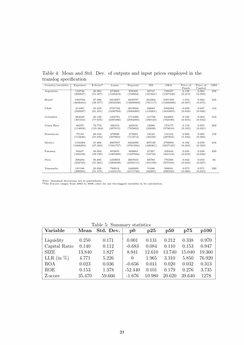
Table 4: Mean and Std. Dev. of outputs and input prices employed in thetranslog specification
Country/variables Expenses Z-Score* Loans Deposits NII OEA Price of Price of OBSFunds Capital
Argentina 152749 20.982 672903 878409 82747 748337 0.109 0.082 338(293837) (51.407) (1348218) (159862) (161821) (1557448) (0.213) (0.059)
Brazil 1383722 27.288 3212067 4230787 252384 5301560 1.074 0.084 535(3636441) (38.477) (9950336) (13000000) (781117) (15400000) (6.507) (0.075)
Chile 411081 55.459 3727192 3619562 82683 1092382 0.059 0.037 154(592297) (61.251) (5240769) (5082460) (110201) (1633905) (0.032) (0.026)
Colombia 262049 35.100 1404781 1714300 121790 644983 0.169 0.064 210(401354) (77.035) (2391686) (2582393) (180123) (762196) (0.816) (0.042)
Costa Rica 66279 72.772 320153 425616 12088 173177 0.110 0.055 202(114858) (121.064) (497015) (765862) (23698) (379610) (0.103) (0.021)
Dominican 75124 29.342 279828 373063 19125 151416 0.680 0.085 159(115846) (31.670) (507883) (714574) (40109) (287855) (5.342) (0.063)
Mexico 1104384 31.868 4967057 6242088 207100 2798891 0.182 0.058 218(1668294) (37.403) (7441757) (9761256) (428361) (5637125) (0.452) (0.050)
Panama 94447 56.002 853835 999884 27397 339442 0.045 0.028 230(160108) (39.730) (1405369) (1527944) (54732) (431514) (0.019) (0.022)
Peru 206494 35.885 1459859 2067655 68783 776308 0.042 0.053 84(232745) (31.361) (1864046) (2533111) (101109) (975164) (0.032) (0.027)
Venezuela 191186 23.928 788014 1440600 51848 506641 0.073 0.071 220(290065) (31.375) (1435133) (2171726) (82265) (686350) (0.066) (0.033)
Note: Standard deviations are in parenthesis.*The Z-score ranges from 2003 to 2008, since we use two-lagged variables in its calculation.
Table 5: Summary statisticsVariable Mean Std. Dev. p0 p25 p50 p75 p100
Liquidity 0.250 0.171 0.001 0.131 0.212 0.338 0.970Capital Ratio 0.140 0.112 -0.683 0.084 0.110 0.153 0.947SIZE 13.840 1.827 8.941 12.610 13.740 15.040 19.360LLR (in %) 4.771 5.226 0 1.965 3.310 5.850 76.920ROA 0.023 0.036 -0.656 0.011 0.020 0.032 0.313ROE 0.153 1.378 -52.440 0.101 0.179 0.276 3.735Z-score 35.470 59.666 -1.676 10.980 20.620 39.640 1278
31
Tab
le6:
Cro
ss-C
orre
lati
onT
able
Var
iable
sZ
-Sco
reSIZ
EL
iquid
ity
Cap
ital
RO
AR
OE
LL
RP
riva
teF
orre
ign
Z-S
core
1.00
0SIZ
E0.
001
1.00
0L
iquid
ity
-0.1
610.
044
1.00
0C
apit
al0.
158
-0.3
430.
025
1.00
0R
OA
0.03
5-0
.022
0.03
30.
407
1.00
0R
OE
0.01
20.
027
0.03
20.
013
0.06
21.
000
LL
R-0
.106
-0.0
650.
105
0.05
4-0
.161
-0.0
631.
000
Pri
vate
0.00
4-0
.233
-0.1
01-0
.037
0.03
9-0
.013
-0.0
041.
000
For
eign
-0.0
470.
092
0.01
0-0
.000
-0.0
600.
003
-0.1
27-0
.697
1.00
0
32
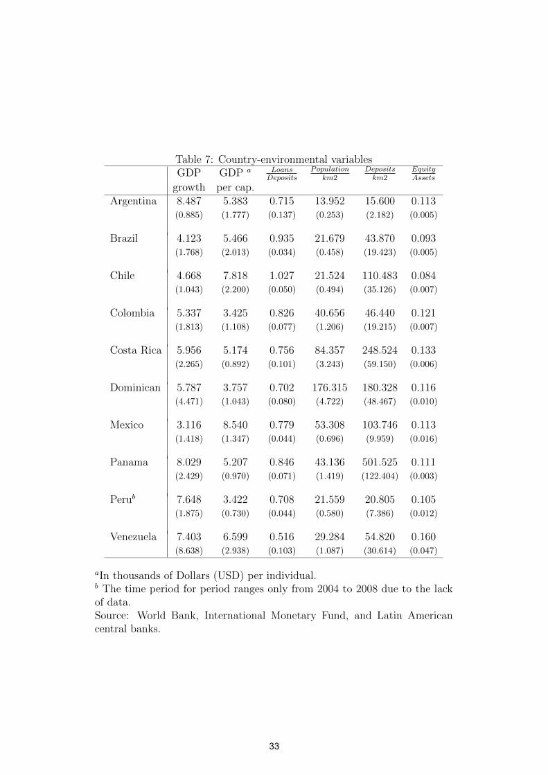
Table 7: Country-environmental variablesGDP GDP a Loans
DepositsPopulation
km2Depositskm2
EquityAssets
growth per cap.Argentina 8.487 5.383 0.715 13.952 15.600 0.113
(0.885) (1.777) (0.137) (0.253) (2.182) (0.005)
Brazil 4.123 5.466 0.935 21.679 43.870 0.093(1.768) (2.013) (0.034) (0.458) (19.423) (0.005)
Chile 4.668 7.818 1.027 21.524 110.483 0.084(1.043) (2.200) (0.050) (0.494) (35.126) (0.007)
Colombia 5.337 3.425 0.826 40.656 46.440 0.121(1.813) (1.108) (0.077) (1.206) (19.215) (0.007)
Costa Rica 5.956 5.174 0.756 84.357 248.524 0.133(2.265) (0.892) (0.101) (3.243) (59.150) (0.006)
Dominican 5.787 3.757 0.702 176.315 180.328 0.116(4.471) (1.043) (0.080) (4.722) (48.467) (0.010)
Mexico 3.116 8.540 0.779 53.308 103.746 0.113(1.418) (1.347) (0.044) (0.696) (9.959) (0.016)
Panama 8.029 5.207 0.846 43.136 501.525 0.111(2.429) (0.970) (0.071) (1.419) (122.404) (0.003)
Perub 7.648 3.422 0.708 21.559 20.805 0.105(1.875) (0.730) (0.044) (0.580) (7.386) (0.012)
Venezuela 7.403 6.599 0.516 29.284 54.820 0.160(8.638) (2.938) (0.103) (1.087) (30.614) (0.047)
aIn thousands of Dollars (USD) per individual.b The time period for period ranges only from 2004 to 2008 due to the lackof data.Source: World Bank, International Monetary Fund, and Latin Americancentral banks.
33
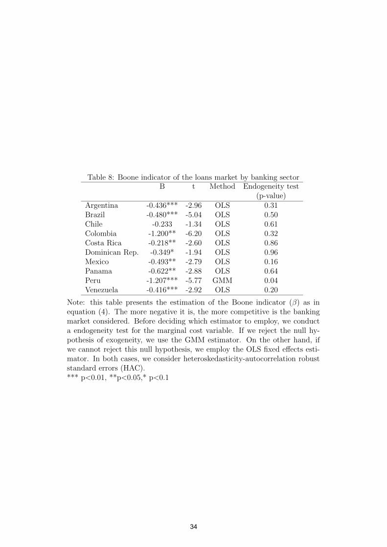
Table 8: Boone indicator of the loans market by banking sectorB t Method Endogeneity test
(p-value)Argentina -0.436*** -2.96 OLS 0.31Brazil -0.480*** -5.04 OLS 0.50Chile -0.233 -1.34 OLS 0.61Colombia -1.200** -6.20 OLS 0.32Costa Rica -0.218** -2.60 OLS 0.86Dominican Rep. -0.349* -1.94 OLS 0.96Mexico -0.493** -2.79 OLS 0.16Panama -0.622** -2.88 OLS 0.64Peru -1.207*** -5.77 GMM 0.04Venezuela -0.416*** -2.92 OLS 0.20
Note: this table presents the estimation of the Boone indicator (β) as inequation (4). The more negative it is, the more competitive is the bankingmarket considered. Before deciding which estimator to employ, we conducta endogeneity test for the marginal cost variable. If we reject the null hy-pothesis of exogeneity, we use the GMM estimator. On the other hand, ifwe cannot reject this null hypothesis, we employ the OLS fixed effects esti-mator. In both cases, we consider heteroskedasticity-autocorrelation robuststandard errors (HAC).*** p<0.01, **p<0.05,* p<0.1
34
Tab
le9:
Boon
esc
ores
ofth
elo
ans
mar
ket
by
ban
kin
gse
ctor
and
tim
eY
ear/
AR
GB
RA
CH
IC
OL
CO
RD
OM
ME
XP
AN
PE
RV
EN
Countr
ies
Boone
tB
oone
tB
oone
tB
oone
tB
oone
tB
oone
tB
oone
tB
oone
tB
oone
tB
oone
t2001
0.3
22*
1.6
8-0
.554***
-5.8
9-0
.221
-1.4
-0.6
97***
-5.4
0-0
.257***
-2.8
40.5
97***
4.3
3-0
.218
-0.8
6-0
.445**
-2.4
5-
--0
.242
-1.6
32002
-0.5
80
-1.5
6-0
.366***
-3.4
5-0
.252
-1.5
4-0
.620***
-3.9
8-0
.216**
-2.5
20.2
86
1.1
3-0
.600***
-3.6
8-0
.677***
-3.4
5-1
.232***
-4.3
8-0
.866***
-3.9
02003
-0.4
29***
-2.6
3-0
.504***
-5.9
7-0
.275
-1.5
9-0
.710***
-4.5
9-0
.285**
-2.3
90.2
92
0.9
2-0
.551***
-3.7
6-0
.700***
-3.3
0-1
.303***
-3.6
3-0
.596***
-4.4
52004
-0.5
90***
-2.6
8-0
.511***
-5.6
1-0
.285
-1.6
4-0
.916***
-6.6
2-0
.298***
-2.9
9-0
.624***
-3.5
3-0
.517***
-3.3
7-0
.751**
-2.3
6-1
.304***
-3.6
5-0
.680***
-4.8
72005
-0.2
62*
-1.7
5-0
.363***
-4.0
4-0
.279
-1.6
4-0
.979***
-7.4
9-0
.282***
-2.8
6-0
.606***
-3.3
8-0
.461***
-3.1
9-0
.585***
-3.1
5-1
.192***
-3.8
3-0
.202
-1.2
72006
-0.3
63***
-3.1
4-0
.461***
-5.3
2-0
.279
-1.6
5-1
.167***
-10.5
9-0
.228**
-2.4
1-0
.975***
-4.0
4-0
.466***
-3.0
4-0
.286**
-2.0
2-1
.230***
-4.0
4-0
.158
-0.9
52007
-0.3
46***
-2.6
8-0
.496***
-4.9
7-0
.250*
-1.6
7-1
.141***
-7.8
6-0
.262**
-2.3
0-1
.591***
-4.1
5-0
.405***
-2.7
8-0
.286
-0.7
6-1
.283***
-4.6
4-0
.140
-0.8
12008
-0.4
71***
-3.7
3-0
.383***
-4.4
8-0
.219
-1.4
9-0
.731***
-5.5
3-0
.166
-1.6
5-1
.366***
-3.1
3-0
.639***
-2.9
3-0
.353
-0.9
9-1
.242***
-5.6
90.9
57***
3.5
1
Model:
OL
SO
LS
OL
SO
LS
OL
SO
LS
OL
SO
LS
GM
MO
LS
Not
e:th
ista
ble
pre
sents
the
esti
mat
ion
ofB
oon
ein
dic
ator
that
dep
end
son
tim
e(β
t)
asin
equ
atio
n(5
).T
he
mor
en
egat
ive
itis
,th
em
ore
com
pet
itiv
eis
the
ban
kin
gm
arke
tat
that
spec
ific
poi
nt
ofti
me.
Bef
ore
dec
idin
gw
hic
hes
tim
ator
toem
plo
y,w
eco
nd
uct
aen
dog
enei
tyte
stfo
rth
em
argi
nal
cost
vari
able
.If
we
reje
ctth
enu
llhyp
oth
esis
ofex
ogen
eity
,w
euse
the
GM
Mes
tim
ator
.O
nth
eot
her
han
d,
ifw
eca
nn
otre
ject
this
nu
llhyp
oth
esis
,w
eem
plo
yth
eO
LS
fixed
effec
tses
tim
ator
.In
bot
hca
ses,
we
con
sider
het
eros
ked
asti
city
-au
toco
rrel
ati
onro
bu
stst
and
ard
erro
rs(H
AC
).**
*p<
0.01
,**
p<
0.05
,*p<
0.1
35
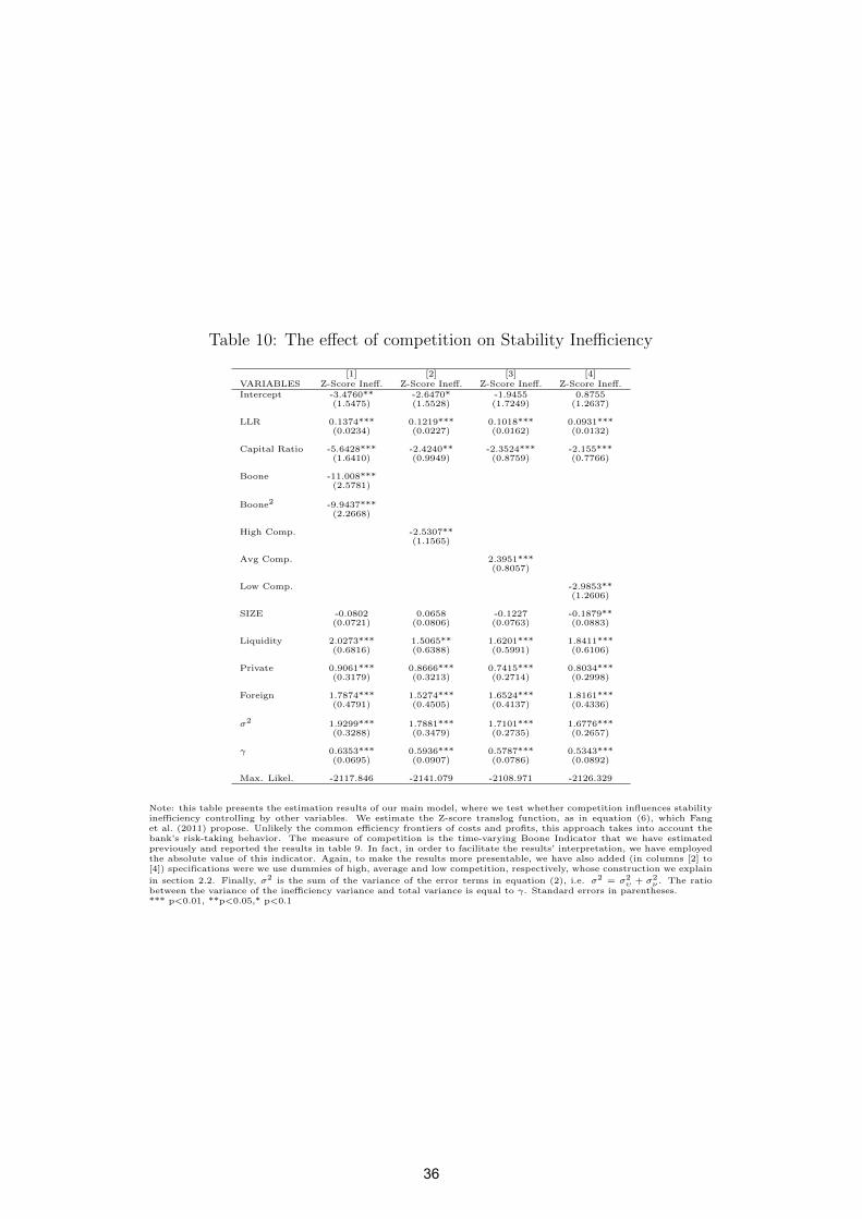
Table 10: The effect of competition on Stability Inefficiency
[1] [2] [3] [4]VARIABLES Z-Score Ineff. Z-Score Ineff. Z-Score Ineff. Z-Score Ineff.Intercept -3.4760** -2.6470* -1.9455 0.8755
(1.5475) (1.5528) (1.7249) (1.2637)
LLR 0.1374*** 0.1219*** 0.1018*** 0.0931***(0.0234) (0.0227) (0.0162) (0.0132)
Capital Ratio -5.6428*** -2.4240** -2.3524*** -2.155***(1.6410) (0.9949) (0.8759) (0.7766)
Boone -11.008***(2.5781)
Boone2 -9.9437***(2.2668)
High Comp. -2.5307**(1.1565)
Avg Comp. 2.3951***(0.8057)
Low Comp. -2.9853**(1.2606)
SIZE -0.0802 0.0658 -0.1227 -0.1879**(0.0721) (0.0806) (0.0763) (0.0883)
Liquidity 2.0273*** 1.5065** 1.6201*** 1.8411***(0.6816) (0.6388) (0.5991) (0.6106)
Private 0.9061*** 0.8666*** 0.7415*** 0.8034***(0.3179) (0.3213) (0.2714) (0.2998)
Foreign 1.7874*** 1.5274*** 1.6524*** 1.8161***(0.4791) (0.4505) (0.4137) (0.4336)
σ2 1.9299*** 1.7881*** 1.7101*** 1.6776***(0.3288) (0.3479) (0.2735) (0.2657)
γ 0.6353*** 0.5936*** 0.5787*** 0.5343***(0.0695) (0.0907) (0.0786) (0.0892)
Max. Likel. -2117.846 -2141.079 -2108.971 -2126.329
Note: this table presents the estimation results of our main model, where we test whether competition influences stabilityinefficiency controlling by other variables. We estimate the Z-score translog function, as in equation (6), which Fanget al. (2011) propose. Unlikely the common efficiency frontiers of costs and profits, this approach takes into account thebank’s risk-taking behavior. The measure of competition is the time-varying Boone Indicator that we have estimatedpreviously and reported the results in table 9. In fact, in order to facilitate the results’ interpretation, we have employedthe absolute value of this indicator. Again, to make the results more presentable, we have also added (in columns [2] to[4]) specifications were we use dummies of high, average and low competition, respectively, whose construction we explain
in section 2.2. Finally, σ2 is the sum of the variance of the error terms in equation (2), i.e. σ2 = σ2υ + σ2
ν . The ratiobetween the variance of the inefficiency variance and total variance is equal to γ. Standard errors in parentheses.*** p<0.01, **p<0.05,* p<0.1
36
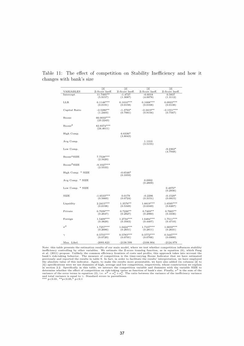
Table 11: The effect of competition on Stability Inefficiency and how itchanges with bank’s size
[2] [2] [2] [2]VARIABLES Z-Score Ineff. Z-Score Ineff. Z-Score Ineff. Z-Score Ineff.Intercept 11.7495** -1.4727 -0.6018 0.5837
(5.9157) (1.3087) (4.0078) (1.3112)
LLR 0.1148*** 0.1010*** 0.1008*** 0.0923***(0.0191) (0.0158) (0.0168) (0.0138)
Capital Ratio -2.5280** -1.3793* -2.2419** -2.1551***(1.2403) (0.7881) (0.9156) (0.7567)
Boone 66.0032***(23.2243)
Boone2 82.9374***(24.4611)
High Comp. 6.6336*(3.8043)
Avg Comp. 1.1310(3.5155)
Low Comp. -9.2362*(4.7948)
Boone*SIZE 7.7528***(2.3420)
Boone2SIZE -9.1027***(2.5533)
High Comp. * SIZE -0.6546*(0.3359)
Avg Comp. * SIZE 0.0992(0.2809)
Low Comp. * SIZE 0.4970*(0.2936)
SIZE -1.6533*** 0.0179 -0.2296 -0.1529*(0.5660) (0.0724) (0.3151) (0.0815)
Liquidity 2.2415*** 1.3576** 1.6619*** 1.6595***(0.6198) (0.5349) (0.6349) (0.6267)
Private 0.7039*** 0.7226** 0.7403** 0.7665**(0.2647) (0.2827) (0.2980) (0.3336)
Foreign 1.5409*** 1.2734*** 1.6484*** 1.7511***(0.3829) (0.3563) (0.4407) (0.4710)
σ2 1.7257*** 1.6424*** 1.7107*** 1.6659***(0.2686) (0.2651) (0.2811) (0.2631)
γ 0.5755*** 0.5783*** 0.5772*** 0.5447***(0.0720) (0.0791) (0.0766) (0.0900)
Max. Likel. -2093.823 -2138.599 -2108.904 -2124.979
Note: this table presents the estimation results of our main model, where we test whether competition influences stabilityinefficiency controlling by other variables. We estimate the Z-score translog function, as in equation (6), which Fanget al. (2011) propose. Unlikely the common efficiency frontiers of costs and profits, this approach takes into account thebank’s risk-taking behavior. The measure of competition is the time-varying Boone Indicator that we have estimatedpreviously and reported the results in table 9. In fact, in order to facilitate the results’ interpretation, we have employedthe absolute value of this indicator. Again, to make the results more presentable, we have also added (in columns [2] to[4]) specifications were we use dummies of high, average and low competition, respectively, whose construction we explainin section 2.2. Specifically in this table, we interact the competition variable and dummies with the variable SIZE todetermine whether the effect of competition on risk-taking varies as function of bank’s size. Finally, σ2 is the sum of thevariance of the error terms in equation (2), i.e. σ2 = σ2
υ + σ2ν . The ratio between the variance of the inefficiency variance
and total variance is equal to γ. Standard errors in parentheses.*** p<0.01, **p<0.05,* p<0.1
37
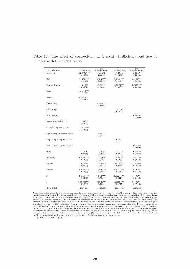
Table 12: The effect of competition on Stability Inefficiency and how itchanges with the capital ratio
[1] [2] [3] [4]VARIABLES Z-Score Ineff. Z-Score Ineff. Z-Score Ineff. Z-Score Ineff.Intercept -14.6270*** -3.0464 -0.7742 0.7067
(3.9837) (2.1282) (1.6239) (1.2264)
LLR 0.1153*** 0.1352*** 0.0848*** 0.0921***(0.0195) (0.0399) (0.0164) (0.0128)
Capital Ratio -10.1520 -3.2417* -3.7974*** -1.9417***(6.5661) (1.9636) (1.3933) (0.7496)
Boone -60.415***(15.736)
Boone2 -62.475***(16.016)
High Comp. -3.1202*(1.8966)
Avg Comp. 1.4375*(0.7501)
Low Comp. 0.8835(1.0209)
Boone*Capital Ratio 52.546**(19.296)
Boone2*Capital Ratio -71.577***(19.455)
High Comp.*Capital Ratio 1.5945(2.5987)
Avg Comp.*Capital Ratio 2.5072(1.736)
Low Comp.*Capital Ratio -29.214**(14.893)
SIZE -0.0670 0.0623 -0.0943 -0.1540**(0.0741) (0.0862) (0.0790) (0.0727)
Liquidity 1.8218*** 1.7446* 1.2260** 1.5313**(0.5407) (0.9361) (0.5357) (0.5654)
Private 0.6354** 0.9799** 0.5780** 0.7519**(0.2732) (0.4246) (0.2744) (0.2948)
Foreign 1.4945*** 1.7388** 1.3014*** 1.6820***(0.3860) (0.6964) (0.4011) (0.4154)
σ2 1.5805*** 1.9437*** 1.5224*** 1.6893***(0.2384) (0.5355) (0.2414) (0.2429)
γ 0.50684*** 0.6223*** 0.5469*** 0.5699***(0.0800) (0.1024) (0.0775) (0.0744)
Max. Likel. -2087.235 -2140.934 -2108.136 -2120.743
Note: this table presents the estimation results of our main model, where we test whether competition influences stabilityinefficiency controlling by other variables. We estimate the Z-score translog function, as in equation (6), which Fanget al. (2011) propose. Unlikely the common efficiency frontiers of costs and profits, this approach takes into account thebank’s risk-taking behavior. The measure of competition is the time-varying Boone Indicator that we have estimatedpreviously and reported the results in table 9. In fact, in order to facilitate the results’ interpretation, we have employedthe absolute value of this indicator. Again, to make the results more presentable, we have also added (in columns [2] to[4]) specifications were we use dummies of high, average and low competition, respectively, whose construction we explainin section 2.2. Specifically in this table, we interact the competition variable and dummies with the variable Capital Ratioto determine whether the effect of competition on risk-taking varies as function of bank’s capital ratio. Finally, σ2 isthe sum of the variance of the error terms in equation (2), i.e. σ2 = σ2
υ + σ2ν . The ratio between the variance of the
inefficiency variance and total variance is equal to γ. Standard errors in parentheses.*** p<0.01, **p<0.05,* p<0.1
38
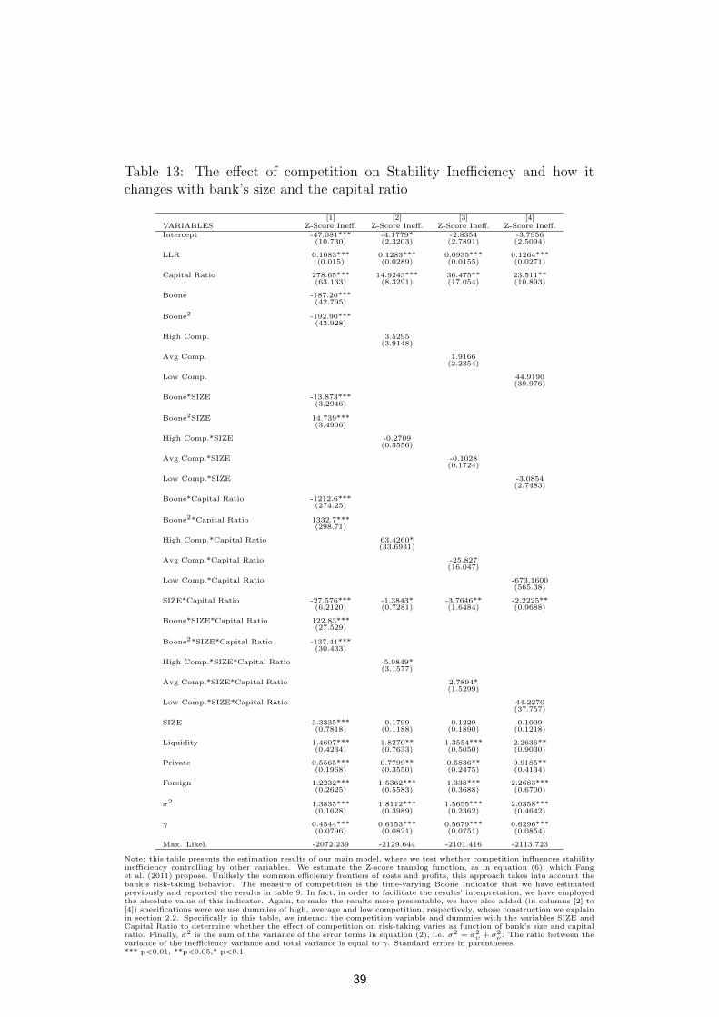
Table 13: The effect of competition on Stability Inefficiency and how itchanges with bank’s size and the capital ratio
[1] [2] [3] [4]VARIABLES Z-Score Ineff. Z-Score Ineff. Z-Score Ineff. Z-Score Ineff.Intercept -47.081*** -4.1779* -2.8354 -3.7956
(10.730) (2.3203) (2.7891) (2.5094)
LLR 0.1083*** 0.1283*** 0.0935*** 0.1264***(0.015) (0.0289) (0.0155) (0.0271)
Capital Ratio 278.65*** 14.9243*** 36.475** 23.511**(63.133) (8.3291) (17.054) (10.893)
Boone -187.20***(42.795)
Boone2 -192.90***(43.928)
High Comp. 3.5295(3.9148)
Avg Comp. 1.9166(2.2354)
Low Comp. 44.9190(39.976)
Boone*SIZE -13.873***(3.2946)
Boone2SIZE 14.739***(3.4906)
High Comp.*SIZE -0.2709(0.3556)
Avg Comp.*SIZE -0.1028(0.1724)
Low Comp.*SIZE -3.0854(2.7483)
Boone*Capital Ratio -1212.6***(274.25)
Boone2*Capital Ratio 1332.7***(298.71)
High Comp.*Capital Ratio 63.4260*(33.6931)
Avg Comp.*Capital Ratio -25.827(16.047)
Low Comp.*Capital Ratio -673.1600(565.38)
SIZE*Capital Ratio -27.576*** -1.3843* -3.7646** -2.2225**(6.2120) (0.7281) (1.6484) (0.9688)
Boone*SIZE*Capital Ratio 122.83***(27.529)
Boone2*SIZE*Capital Ratio -137.41***(30.433)
High Comp.*SIZE*Capital Ratio -5.9849*(3.1577)
Avg Comp.*SIZE*Capital Ratio 2.7894*(1.5299)
Low Comp.*SIZE*Capital Ratio 44.2270(37.757)
SIZE 3.3335*** 0.1799 0.1229 0.1099(0.7818) (0.1188) (0.1890) (0.1218)
Liquidity 1.4607*** 1.8270** 1.3554*** 2.2636**(0.4234) (0.7633) (0.5050) (0.9030)
Private 0.5565*** 0.7799** 0.5836** 0.9185**(0.1968) (0.3550) (0.2475) (0.4134)
Foreign 1.2232*** 1.5362*** 1.338*** 2.2683***(0.2625) (0.5583) (0.3688) (0.6700)
σ2 1.3835*** 1.8112*** 1.5655*** 2.0358***(0.1628) (0.3989) (0.2362) (0.4642)
γ 0.4544*** 0.6153*** 0.5679*** 0.6296***(0.0796) (0.0821) (0.0751) (0.0854)
Max. Likel. -2072.239 -2129.644 -2101.416 -2113.723
Note: this table presents the estimation results of our main model, where we test whether competition influences stabilityinefficiency controlling by other variables. We estimate the Z-score translog function, as in equation (6), which Fanget al. (2011) propose. Unlikely the common efficiency frontiers of costs and profits, this approach takes into account thebank’s risk-taking behavior. The measure of competition is the time-varying Boone Indicator that we have estimatedpreviously and reported the results in table 9. In fact, in order to facilitate the results’ interpretation, we have employedthe absolute value of this indicator. Again, to make the results more presentable, we have also added (in columns [2] to[4]) specifications were we use dummies of high, average and low competition, respectively, whose construction we explainin section 2.2. Specifically in this table, we interact the competition variable and dummies with the variables SIZE andCapital Ratio to determine whether the effect of competition on risk-taking varies as function of bank’s size and capitalratio. Finally, σ2 is the sum of the variance of the error terms in equation (2), i.e. σ2 = σ2
υ + σ2ν . The ratio between the
variance of the inefficiency variance and total variance is equal to γ. Standard errors in parentheses.*** p<0.01, **p<0.05,* p<0.1
39
Banco Central do Brasil
Trabalhos para Discussão Os Trabalhos para Discussão do Banco Central do Brasil estão disponíveis para download no website
http://www.bcb.gov.br/?TRABDISCLISTA
Working Paper Series
The Working Paper Series of the Central Bank of Brazil are available for download at http://www.bcb.gov.br/?WORKINGPAPERS
221 Financial Instability and Credit Constraint: evidence from the cost of
bank financing Bruno S. Martins
Nov/2010
222 O Comportamento Cíclico do Capital dos Bancos Brasileiros R. A. Ferreira, A. C. Noronha, B. M. Tabak e D. O. Cajueiro
Nov/2010
223 Forecasting the Yield Curve with Linear Factor Models Marco Shinobu Matsumura, Ajax Reynaldo Bello Moreira and José Valentim Machado Vicente
Nov/2010
224 Emerging Floaters: pass-throughs and (some) new commodity currencies Emanuel Kohlscheen
Nov/2010
225 Expectativas Inflacionárias e Inflação Implícita no Mercado Brasileiro Flávio de Freitas Val, Claudio Henrique da Silveira Barbedo e Marcelo Verdini Maia
Nov/2010
226 A Macro Stress Test Model of Credit Risk for the Brazilian Banking Sector Francisco Vazquez, Benjamin M.Tabak and Marcos Souto
Nov/2010
227 Uma Nota sobre Erros de Previsão da Inflação de Curto Prazo Emanuel Kohlscheen
Nov/2010
228 Forecasting Brazilian Inflation Using a Large Data Set Francisco Marcos Rodrigues Figueiredo
Dec/2010
229 Financial Fragility in a General Equilibrium Model: the Brazilian case Benjamin M. Tabak, Daniel O. Cajueiro and Dimas M. Fazio
Dec/2010
230 Is Inflation Persistence Over? Fernando N. de Oliveira and Myrian Petrassi
Dec/2010
231 Capital Requirements and Business Cycles with Credit Market Imperfections P. R. Agénor, K. Alper and L. Pereira da Silva
Jan/2011
232 Modeling Default Probabilities: the case of Brazil Benjamin M. Tabak, Daniel O. Cajueiro and A. Luduvice
Jan/2011
40
233 Emerging Floaters: pass-throughs and (some) new commodity currencies Emanuel Kohlscheen
Jan/2011
234 Cyclical Effects of Bank Capital Requirements with Imperfect Credit Markets Pierre-Richard Agénor and Luiz A. Pereira da Silva
Jan/2011
235 Revisiting bank pricing policies in Brazil: Evidence from loan and deposit markets Leonardo S. Alencar
Mar/2011
236 Optimal costs of sovereign default Leonardo Pio Perez
Apr/2011
237 Capital Regulation, Monetary Policy and Financial Stability P.R. Agénor, K. Alper, and L. Pereira da Silva
Apr/2011
238 Choques não Antecipados de Política Monetária e a Estrutura a Termo das Taxas de Juros no Brasil Fernando N. de Oliveira e Leonardo Ramos
Abr/2011
239 SAMBA: Stochastic Analytical Model with a Bayesian Approach Marcos R. de Castro, Solange N. Gouvea, André Minella, Rafael C. Santos and Nelson F. Souza-Sobrinho
Apr/2011
240 Fiscal Policy in Brazil through the Lens of an Estimated DSGE Model Fabia A. de Carvalho and Marcos Valli
Apr/2011
241 Macro Stress Testing of Credit Risk Focused on the Tails Ricardo Schechtman and Wagner Piazza Gaglianone
May/2011
242 Determinantes do Spread Bancário Ex-Post no Mercado Brasileiro José Alves Dantas, Otávio Ribeiro de Medeiros e Lúcio Rodrigues Capelletto
Maio/2011
243 Economic Activity and Financial Institutional Risk: an empirical analysis for the Brazilian banking industry Helder Ferreira de Mendonça, Délio José Cordeiro Galvão and Renato Falci Villela Loures
May/2011
244 Profit, Cost and Scale Eficiency for Latin American Banks: concentration-performance relationship Benjamin M. Tabak, Dimas M. Fazio and Daniel O. Cajueiro
May/2011
245 Pesquisa Trimestral de Condições de Crédito no Brasil Clodoaldo Aparecido Annibal e Sérgio Mikio Koyama
Jun/2011
246 Impacto do Sistema Cooperativo de Crédito na Eficiência do Sistema Financeiro Nacional Michel Alexandre da Silva
Ago/2011
247 Forecasting the Yield Curve for the Euro Region Benjamim M. Tabak, Daniel O. Cajueiro and Alexandre B. Sollaci
Aug/2011
248 Financial regulation and transparency of information: first steps on new land Helder Ferreira de Mendonça, Délio José Cordeiro Galvão and Renato Falci Villela Loures
Aug/2011
41
249 Directed clustering coefficient as a measure of systemic risk in complex banking networks B. M. Tabak, M. Takami, J. M. C. Rocha and D. O. Cajueiro
Aug/2011
250 Recolhimentos Compulsórios e o Crédito Bancário Brasileiro
Paulo Evandro Dawid e Tony Takeda
Ago/2011
251 Um Exame sobre como os Bancos Ajustam seu Índice de Basileia no Brasil Leonardo S. Alencar
Ago/2011
252 Comparação da Eficiência de Custo para BRICs e América Latina Lycia M. G. Araujo, Guilherme M. R. Gomes, Solange M. Guerra e Benjamin M. Tabak
Set/2011
253 Bank Efficiency and Default in Brazil: causality tests Benjamin M. Tabak, Giovana L. Craveiro and Daniel O. Cajueiro
Oct/2011
254 Macroprudential Regulation and the Monetary Transmission Mechanism Pierre-Richard Agénor and Luiz A. Pereira da Silva
Nov/2011
255 An Empirical Analysis of the External Finance Premium of Public Non-Financial Corporations in Brazil Fernando N. de Oliveira and Alberto Ronchi Neto
Nov/2011
256 The Self-insurance Role of International Reserves and the 2008-2010 Crisis Antonio Francisco A. Silva Jr
Nov/2011
257 Cooperativas de Crédito: taxas de juros praticadas e fatores de viabilidade Clodoaldo Aparecido Annibal e Sérgio Mikio Koyama
Nov/2011
258 Bancos Oficiais e Crédito Direcionado – O que diferencia o mercado de crédito brasileiro? Eduardo Luis Lundberg
Nov/2011
259 The impact of monetary policy on the exchange rate: puzzling evidence from three emerging economies Emanuel Kohlscheen
Nov/2011
260 Credit Default and Business Cycles: an empirical investigation of Brazilian retail loans Arnildo da Silva Correa, Jaqueline Terra Moura Marins, Myrian Beatriz Eiras das Neves and Antonio Carlos Magalhães da Silva
Nov/2011
42