Tm

AU

a

ARRA

KAMEC

1

tGi(m(1tt(

sleec(pP

r

0d

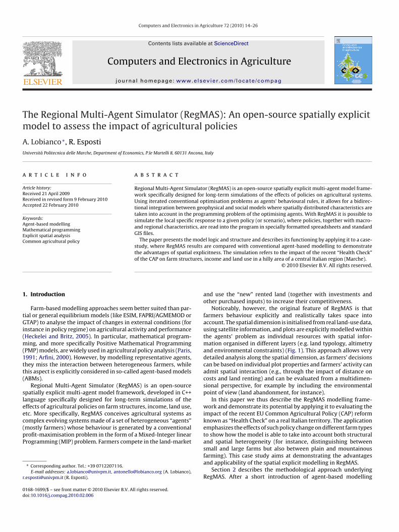
Computers and Electronics in Agriculture 72 (2010) 14–26

Contents lists available at ScienceDirect

Computers and Electronics in Agriculture

journa l homepage: www.e lsev ier .com/ locate /compag

he Regional Multi-Agent Simulator (RegMAS): An open-source spatially explicitodel to assess the impact of agricultural policies

. Lobianco ∗, R. Espostiniversità Politecnica delle Marche, Department of Economics, P.le Martelli 8, 60131 Ancona, Italy

r t i c l e i n f o

rticle history:eceived 21 April 2009eceived in revised form 9 February 2010ccepted 22 February 2010

eywords:

a b s t r a c t

Regional Multi-Agent Simulator (RegMAS) is an open-source spatially explicit multi-agent model frame-work specifically designed for long-term simulations of the effects of policies on agricultural systems.Using iterated conventional optimisation problems as agents’ behavioural rules, it allows for a bidirec-tional integration between geophysical and social models where spatially distributed characteristics aretaken into account in the programming problem of the optimising agents. With RegMAS it is possible to

gent-based modellingathematical programming

xplicit spatial analysisommon agricultural policy

simulate the local specific response to a given policy (or scenario), where policies, together with macro-and regional characteristics, are read into the program in specially formatted spreadsheets and standardGIS files.

The paper presents the model logic and structure and describes its functioning by applying it to a case-study, where RegMAS results are compared with conventional agent-based modelling to demonstratethe advantages of spatial explicitness. The simulation refers to the impact of the recent “Health Check”

ures,

of the CAP on farm struct

. Introduction

Farm-based modelling approaches seem better suited than par-ial or general equilibrium models (like ESIM, FAPRI/AGMEMOD orTAP) to analyse the impact of changes in external conditions (for

nstance in policy regime) on agricultural activity and performanceHeckelei and Britz, 2005). In particular, mathematical program-

ing, and more specifically Positive Mathematical ProgrammingPMP) models, are widely used in agricultural policy analysis (Paris,991; Arfini, 2000). However, by modelling representative agents,hey miss the interaction between heterogeneous farmers, whilehis aspect is explicitly considered in so-called agent-based modelsABMs).

Regional Multi-Agent Simulator (RegMAS) is an open-sourcepatially explicit multi-agent model framework, developed in C++anguage specifically designed for long-term simulations of theffects of agricultural policies on farm structures, income, land use,

tc. More specifically, RegMAS conceives agricultural systems asomplex evolving systems made of a set of heterogeneous “agents”mostly farmers) whose behaviour is generated by a conventionalrofit-maximisation problem in the form of a Mixed-Integer linearrogramming (MIP) problem. Farmers compete in the land-market

∗ Corresponding author. Tel.: +39 0712207116.E-mail addresses: a.lobianco@univpm.it, antonello@lobianco.org (A. Lobianco),

.esposti@univpm.it (R. Esposti).

168-1699/$ – see front matter © 2010 Elsevier B.V. All rights reserved.oi:10.1016/j.compag.2010.02.006

income and land use in a hilly area of a central Italian region (Marche).© 2010 Elsevier B.V. All rights reserved.

and use the “new” rented land (together with investments andother purchased inputs) to increase their competitiveness.

Noticeably, however, the original feature of RegMAS is thatfarmers behaviour explicitly and realistically takes space intoaccount. The spatial dimension is initialised from real land-use data,using satellite information, and plots are explicitly modelled withinthe agents’ problem as individual resources with spatial infor-mation organised in different layers (e.g. land typology, altimetryand environmental constraints) (Fig. 1). This approach allows verydetailed analysis along the spatial dimension, as farmers’ decisionscan be based on individual plot properties and farmers’ activity canadmit spatial interaction (e.g., through the impact of distance oncosts and land renting) and can be evaluated from a multidimen-sional perspective, for example by including the environmentalpoint of view (land abandonment, for instance).

In this paper we thus describe the RegMAS modelling frame-work and demonstrate its potential by applying it to evaluating theimpact of the recent EU Common Agricultural Policy (CAP) reformknown as “Health Check” on a real Italian territory. The applicationemphasizes the effects of such policy change on different farm typesto show how the model is able to take into account both structuraland spatial heterogeneity (for instance, distinguishing between

small and large farms but also between plain and mountainousfarming). This case study aims at demonstrating the advantagesand applicability of the spatial explicit modelling in RegMAS.

Section 2 describes the methodological approach underlyingRegMAS. After a short introduction of agent-based modelling

A. Lobianco, R. Esposti / Computers and Electronics in Agriculture 72 (2010) 14–26 15

case-s

atmsttiffi

2

2

cPnWti(or

lcpmab

the Mediterranean agriculture.

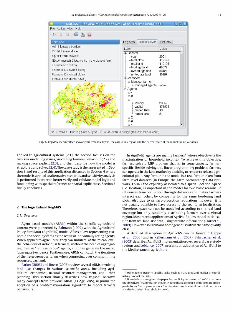
Fig. 1. RegMAS user interface showing the available layers, the

pplied to agricultural systems (2.1), the section focuses on thewo key modelling issues, modelling farmers behaviour (2.2) and

aking space explicit (2.3), and then describe how the model istructured and solved (2.4). The case-study is then presented in Sec-ion 3 and results of this application discussed in Section 4 wherehe model is applied to alternative scenarios and sensitivity analysiss performed in order to better verify and validate model logic andunctioning with special reference to spatial explicitness. Section 5nally concludes.

. The logic behind RegMAS

.1. Overview

Agent-based models (ABMs) within the specific agriculturalontext were pioneered by Balmann (1997) with the Agriculturalolicy Simulator (AgriPoliS) model. ABMs allow representing eco-omic and social systems as the result of individually acting agents.hen applied to agriculture, they can simulate, at the micro-level,

he behaviour of individual farmers, without the need of aggregat-ng them in “representative” agents, and then generate the macroaggregate)-evidence. Furthermore, ABMs can catch the iterationsf the heterogeneous farms when competing over common finiteesources, e.g. land.

Parker (2003) and Boero (2006) review several ABMs involvingand use changes in various scientific areas, including agri-ultural economics, natural resource management, and urbanlanning. This section shortly describes how RegMAS borrowsany concepts from previous ABMs (as AgriPoliS), in primis the

doption of a profit-maximisation algorithm to model farmersehaviours.

tudy region and the current state of the model’s main variables.

In AgriPoliS agents are mainly farmers1 whose objective is themaximisation of household income.2 To achieve this objective,farmers solve a MIP problem that is, in some aspects, farmer-specific. Beside solving this linear programming problem, farmerscan operate in the land market by deciding to rent or to release agri-cultural plots. Any farmer in the model is a real farmer taken fromfarm-level datasets (in Europe, the Farm Accountancy Data Net-work, FADN) and explicitly associated to a spatial location. Space(i.e. location) is important in the model for two basic reasons: itinfluences transport costs (through distance) and makes farmersinteract each other, by competing for the same bordering landplots. Also due to privacy-protection regulations, however, it isnot usually possible to have access to the real farm localisation.Therefore, space can not be modelled according to the real landcoverage but only randomly distributing farmers over a virtualregion. Most recent applications of AgriPoliS allow model initialisa-tion from real land-use data, using satellite information (Piorr et al.,2009). However soil remains homogeneous within the same qualityclass.

A detailed description of AgriPoliS can be found in Happeet al. (2006) and in Kellermann et al. (2007). Sahrbacher et al.(2005) describes AgriPoliS implementation over several case-studyregions and Lobianco (2007) presents an adaptation of AgriPoliS to

1 Other agents perform specific tasks, such as managing land market or coordi-nating product markets.

2 Nonetheless, throughout the paper for simplicity we use term “profit” to expressthe objective of maximisation though in agricultural context it could be more appro-priate to use “farm gross revenue” as objective function or, if household activitiesare also included, “household income”.

1 Elect

2

noptaaair(eoeotosotAptt

h

wmad

tIcaedma

lotemc

ar

tbt

6 A. Lobianco, R. Esposti / Computers and

.2. RegMAS: modelling farmers behaviour

RegMAS uses Mixed Integer linear Programming (MIP) tech-iques to derive farmers behaviours, with profit maximisation asbjective function. There is no real alternative to mathematicalrogramming in modelling farm behaviour over such disaggrega-ion of activities and heterogeneity. Any parametric estimation ofmore flexible technology would be, in fact, unaffordable.3 It is

lso true that, within mathematical programming techniques, validlternative solutions to conventional linear programming do existn modelling individual behaviour: multiple goal programming,ecursive multi-period programming, dynamic programming, etc.Hazell and Norton, 1986; Romero and Rehman, 2003). Here, how-ver, a simple linear profit maximisation problem is adopted notnly because it is the prevalent approach in agricultural policy mod-lling (Ellis et al., 1991; Happe et al., 2008). It also has the advantagef flexibility, as it can account for the whole range of farm activi-ies, from growing specific crops to investing in new machineryr hiring new labour units. Moreover, it is computationally fea-ible within an agent-based contest where each agent has its ownbjective function and further computational effort is demanded byhe spatial-explicit functioning of the model as illustrated below.

final advantage of the MIP is that the introduction of integerarameters allows scale effects to emerge in the model, thus let-ing farmers evolve their response and performance on the basis ofheir economic and physical size included land rental behaviour.4

Any farmer autonomously makes his own decisions by solvingis own MIP problem:

maxxiY =

C+I∑i=1

(GMi ∗ xi)

s.t.C+I∑i=1

ai,j ∗ xi ≤ bj ∀j = 1, . . . , J

xi ≥ 0 ∀i = 1, . . . , C + Ixi ∈ int ∀i = C + 1, . . . , C + I

(1)

here i, activities index; Y, profit; j, resources index; GMi, grossargins; C, continuous activities; bj , capacities (RHS); I, integer

ctivities; ai,j , technical coefficients; J, resource constraints; xi, pro-uction quantities (argument of the maximisation)

The resource and activity sets are open: the RegMAS user is freeo include (or exclude) further individual activities and resources.n the current version, we implement within the model all typi-al activities and resources in running a farm, financial and labourctivities included. While in specialised linear-programming mod-ls these activities can be very detailed, in ABMs the presence ofifferent types of farmers, for any of which a specific program-ing problem has to be solved, makes the analysis limited to more

ggregated activities.Farmers maximise their profit any time they bid to rent a new

and plot (2.3.2) in order to calculate the respective shadow price,r any time they plan a new investment, or decide the produc-

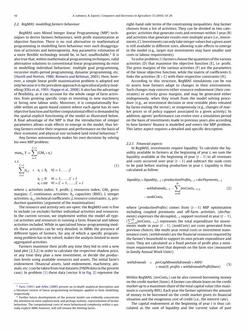
ion levels using available resources and assets. The initial farm’sndowment (financial assets, land endowment, machinery, ani-als, etc.) can be taken from real datasets (FADN data in the present

ase). In problem (1) these data (vector A in Fig. 2) represent the

3 Paris (1991) and Arfini (2000) present an in-depth analytical description andliterature review of linear programming techniques applied to farm modelling,

espectively.4 Further future developments of the present model can evidently concentrate

he attention on more sophisticated, and perhaps realistic, representation of farmerehaviour. The computational costs of more behavioural complexity within a spa-ially explicit ABM, however, will still remain the limiting factor.

ronics in Agriculture 72 (2010) 14–26

right-hand-side terms of the constraining inequalities. Any farmerchooses from a list of activities. They can be divided in two cate-gories: activities that generate costs and revenues within 1 year (B)and activities that generate results over multiple years (i.e., invest-ments, C). Investments can only take integer values but a given assetis still available in different sizes, allowing scale-effects to emergein the model (e.g., larger-size investments may have smaller unitcosts or labour requirements).

To solve problem (1) farmers choose the quantities of the variousactivities (D) that maximise the objective function (E), i.e. profit.The gross margins of the various activities (F) are the parametersof the linear objective function, while the matrix of coefficients Glinks the activities (B + C) with their respective constraints (H).

According to this structure, RegMAS simulations can be runto assess how farmers adapt to changes in their environment.Such changes may concern either resource endowment (their con-straints) or activity gross margins, and may be generated eitherendogenously, when they result from the model solving proce-dure (e.g., an investment decision or new rentable plots releasedby farms exiting the sector), or exogenously (e.g., changes of mar-ket prices or of policy support associated to a given activity). Inaddition, agents’ performance can evolve over a simulation periodon the basis of investments made in previous years also accordingto how farmers’ finance is modelled and enters the MIP problem.This latter aspect requires a detailed and specific description.

2.2.1. Financial aspectsIn RegMAS, investments require liquidity. To calculate the liq-

uidity available to farmers at the beginning of year t, we sum theliquidity available at the beginning of year (t − 1) to all revenuesand costs occurred over year (t − 1) and subtract the sunk coststo be paid before starting production in year t. Liquidity is thuscalculated as follow:

liquidityt= liquidityt−1+productionProfitst−1+decPaymentst−1

− withdrawalst−1 −N∑

n=0

invCostst−1,n

− sunkCostst

(2)

where (productionProfits) comes from (t − 1) MIP optimisationincluding coupled premiums and off-farm activities. (decPay-ments) expresses the decoupledt−1 support received in year (t − 1).(∑N

n=0invCostst−1,n) represents the total expenditure for invest-ments made in year (t − 1). (sunkCosts) are costs generated fromprevious choices, like multi-year rental costs or investment main-tenance costs. (withdrawals) are the financial resources required bythe farmer’s household to support its own private expenditure andcosts. They are calculated as a fixed portion of profit plus a mini-mum requirement level that depends on the farm size (measuredin family Annual Work Units):

withdrawals = perCapMinwithdrawals ∗ AWU+ max(0, profits ∗ withdrawalsProfitShare)

(3)

Within RegMAS, (invCostst) can be also covered borrowing moneyon the credit market (loans). A farmer can obtain loans on the credit

market up to a maximum share of the total capital value (this maxi-mum is currently 80%). Each year the farmer optimises the amountof money to be borrowed on the credit market given its financialsituation and the exogenous cost of credit (i.e., the interest rate).

The capital endowment at the beginning of year t is thus cal-culated as the sum of liquidity and the current value of past

A. Lobianco, R. Esposti / Computers and Electronics in Agriculture 72 (2010) 14–26 17

Integ

i

c

wdcsortn

2

emcthnar

2

micfipmt

d

Fig. 2. Example of the agent’s Mixed

nvestments5:

apitalt = liquidityt +I∑

i=0

investmentCurrentValuei,t (4)

ith I is the number of own capital goods (assets). The realepreciation of different investment objects may depend from theharacteristics of the investment itself, but in the current ver-ion of the model the investment value linearly decreases for allbject types. Therefore, due to the presence of loans, (4) actuallyepresents total capital as combination of debt and equity capi-al under the aforementioned constraint that the debt capital canever exceed 80%.

.3. RegMAS: making space explicit and real

As AgriPoliS, RegMAS has a spatial dimension, that is, it consid-rs the spatial heterogeneity in such a way that, for example, theodel can associate a different rental price to each plot and, thus,

an investigate possible land abandonment even when land cultiva-ion is profitable, on average profitable. Differently from AgriPoliS,owever, this spatial dimension is fully explicit, in the sense that,ot only plots are initialised from real cartographic data, but theyre also explicitly modelled in the decision matrix as individualesources, without the need of aggregating them in soil classes.

.3.1. Region initialisationBefore running the simulation, the model must fix the environ-

ent where the simulation will be generated. This environmentncludes different dimensions: the legislative (subsidies, legalonstraints, etc.), the biophysical (agronomic and technical coef-

cients) and, finally, the economic dimension (factor and productrices). Then, individual farmers can be created, positioned in theodelled space and granted with the tools and resources they need

o operate (e.g. land, machinery and financial resources).

5 Land is not included in this calculation as it is directly read from the farmers’ata file and its endowment never depreciates.

er Programming Problem (excerpt).

Unfortunately, detailed data on all the individual farms (micro-data) within a given region all are often unknown (sometimes forprivacy reasons) while aggregate (macro-) data (for instance, sizedistribution) are usually available (e.g. from Census). Therefore,to re-create the simulation region, the model uses sample farms,for which detailed data are available (in the present case, farmsbelonging to the FADN), then weighed with a scaling coefficientin a such a way that the difference between the aggregate figuresof the simulated region and of the real region is minimised (Eq.(5))6:

minUCn≥0

K∑k=1

⎛⎜⎜⎜⎜⎝

N∑n=1

(FADNn,k ∗ UCn)

REGIOk− 1

⎞⎟⎟⎟⎟⎠

2

(5)

whereIndices Variables

n = {1, . . . , N} individual farms FADNn,k= FADN datak = {1, . . . , K} macro-characteristics REGIOk= regional aggregate data

UCn= “upscaling” coefficient (argumentof the minimisation)

2.3.2. Land allocation, land market and transport costsAfter region initialisation, an obvious problem when dealing

with spatially explicit agent based models concerns the locali-sation of agents and of their spatial objects. As there is alreadyan informative layer, consisting of the real land use (the CorineLand Cover database), we need to make the model consistent withthis layer, by placing farms over it. Firstly, farms are assigned arandom location selecting a plot compatible with their activities,

starting from the less common. The simple idea is that “rare” landuses have the precedence over more common land uses to min-imise distance between such plots and the farmsteads. Hence, ifa farm has, for example, both plots with fruit plantings and plots

6 This procedure is called “upscaling” and it is well documented in Kellermann etal. (2007), while a practical implementation is discussed in Sahrbacher et al. (2005).

1 Elect

wffto

apiplf

tDwadRaafpat

wihppS

isftohvpbftpwittfaahts

bfipo

2

la

Modelling Language (UML) diagram with the main classes and theirrelations.

While this approach allows for rapid development of differentagent types (as only specific characteristics need to be modelled),

7 The Reference Manual has a pseudo-code that details the stepsthe model does to add activities to the MIP problem, available at

8 A. Lobianco, R. Esposti / Computers and

ith arable crops, the farmstead position will correspond to theruit plantings. Subsequently, plots are assigned to the closestarm that has still an un-assigned capacity for that specific soilype, giving precedence to owned plots in comparison to rentednes.

Such land allocation is not, in fact, an optimisation algorithms plots are not assigned to farms in such a way that the totallots X farmsteads distance is minimised. After all, the real worldtself is far from being an optimal land allocation across farms, ashysical boundaries and hereditary rules sometimes split the farm

and endowment in several scattered plots often generating a fairlyragmented allocation.

This initial land allocation across farms, however, is not defini-ive. During model simulation farmers can bid to rent new plots.ifferent assumptions on modelling land market can be madeithin an ABM (Kellermann et al., 2008). In the present case, we

ssume a rental market made up of fixed-term contracts whoseuration is randomly chosen within a fixed interval. In practice,egMAS does not allow direct farmer-to-farmer renting contracts,s farmers can only rent land from an anonymous intermediategent that operates in the land market collecting plots released byarms exiting the business, in addition to the initial pool of rentablelots. This agent makes all these plots available to farmers throughbid where only the farm offering the highest price eventually rents

he plot.Any farmer associates a shadow price to any rentable plot and

hen asked to bid he offers a fraction of this shadow price to takento account both fixed and variable transaction costs and over-eads. The shadow price for any rentable plot is simply calculatederforming two MIP optimisation problems, with and without thelot, and calculating the difference between the two profits (seeection 2.2).

In existing ABMs, like AgriPoliS, land heterogeneity only consistsn different soil types; therefore, plots are homogeneous within theame soil type and farmers are guaranteed to place the highest bidor any certain soil type on the closest plot. This allows these modelso speed up the algorithm code of the land rental market. RegMAS,n the contrary, works with real land-use data therefore plots areeterogeneous also within soil types thus making such algorithmsery computationally demanding (all bid from any farmer on anylots should be collected). To limit the computational complexityut also to add more realism to land market functioning, there-ore, RegMAS offers the option to restrict the bidding process tohe farmers operating within a given distance from the rentablelots; the exact number of bidders (that is, the spatial range overhich any farmer can rent land) is a parameter calibrated accord-

ng to the transport costs: the higher the transport costs, the lowerhe likelihood that a given farm may offer a successful bid (thus,he smaller the range over which he can operate). This is a criticalorm through which space enters the model: distance and costsssociated to it affects the capacity of a farm to rent new landnd, thus, to afford a better economic performance. Symmetrically,eterogeneity of land allows to take into account local plot charac-eristics in forming plot rental prices (and, eventually, in their rentaltatus).

Once the rentable plot is assigned to the farm that won theid a new rental contract is established for a random (and, then,xed) period (the RegMAS user can establish the duration) and thelot, eventually associated to its spatial objects, enters the farmer’sptimisation problem as a new resource.

.3.3. The spatial dimension in the optimisation problemDue to such spatial explicitness, the farmer maximisation prob-

em 1 changes as it takes into account plots as individual resourcesnd each spatial activity is specified for each plot. The optimisation

ronics in Agriculture 72 (2010) 14–26

problem becomes:

maxxiY =

N+S∗P∑i=1

(GMi ∗ xi)

s.t.N+S∗P∑

i=1

ai,j ∗ xi ≤ bj ∀j = 1, . . . , R + P

bj = 1 ∀j = R + 1, . . . , R + Pai,j = 1 ∀i > N ∨ i = N + (j − R)xi ≥ 0 ∀i = 1, . . . , N + S ∗ P

(6)

where i, activities index; Y, profit; j, resources index; GMi, grossmargins; N, non-spatial activities; ai,j , technical coefficients; S, spa-tial activities; bj , capacities (RHS); R, constraining resources; xi,production quantities (argument of the maximisation); P, individ-ual plots.

If the number of plots available to a farmer increases, however,the problem matrices is expected to grow to a size hardly man-ageable even for modern calculators. Therefore, RegMAS followsa sort of “filtering” procedure that, before adding the activities tothe matrix, checks for consistency of any activity with the plot landuse and eventually with the presence of the necessary objects (anexample could be that wine growing activity could be made only onsuitable land with planted vineyards).7 Despite the higher compu-tational costs, using individual plots in the decision problem allowsspatial activities to be evaluated by farmers on the basis of charac-teristics of their associated plot. This means that farmers can takeaccount of transport costs associated to distance of a given plot fromthe farmstead and of plot’s altitude (the hypothesis being that grossmargins declines with altitude). This GIS-alike functionality allowsa full linkage between the economic and the geophysical parts ofthe model.

Similar advantages arise on the output side: when the land useremains implicit in the matrix decision matrix (e.g. farmers are pre-sented with the “agricultural land” total resource rather than witheach individual plots) the spatial location of production remainundefined.8 When, on the contrary, the farm optimises a matrixwith an activity X plot structure, the model can allocate the corre-sponding chosen activity to its associated plot.

2.4. RegMAS: model structure and solving

RegMAS has been designed from the ground up to explicitly con-sider farmers as one specific type among several possible types ofagents. “Farmer” agents are derived from a more general type of“spatial” agents that is, in turn, derived from a “basic” type. Eachagent type has its own “manager” agent that interacts with a “SuperAgent Manager”. The former is a sort of “agent-side” interface whilethe latter implements the same interface on the program “core-side”. In this way, the model core does not need to “know” theagents internal logic. Fig. 3 depicts the organisation of the modelframework at the program level by providing the RegMAS Unified

http://regmas.org/doc/referenceManual/html/classOpt.html.8 Various algorithms could be used (ex-post) to assign production to a particu-

lar plot. One of them is discussed in Brady et al. (2009). It assumes that farmers,given a certain mix of production activities, try to spread them in the smallest pos-sible number of fields, maximising their size. However, land is still considered fullyhomogeneous within the same soil type.

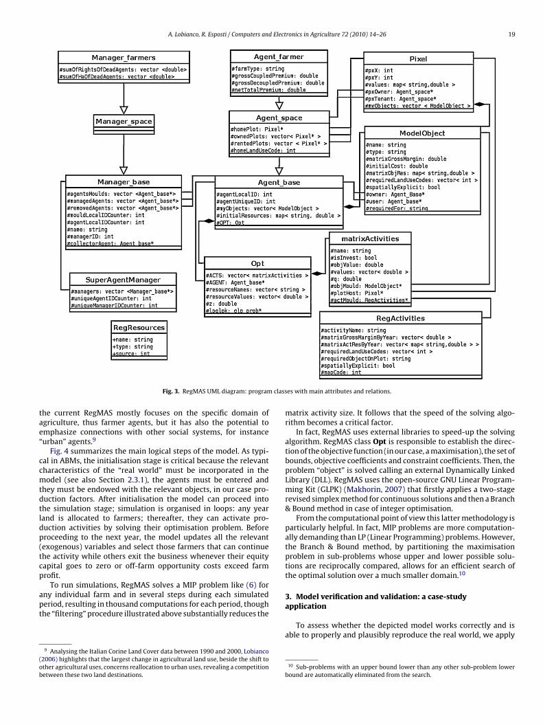
A. Lobianco, R. Esposti / Computers and Electronics in Agriculture 72 (2010) 14–26 19

class

tae“

ccmtdtldp(tcp

apt

(ob

Fig. 3. RegMAS UML diagram: program

he current RegMAS mostly focuses on the specific domain ofgriculture, thus farmer agents, but it has also the potential tomphasize connections with other social systems, for instanceurban” agents.9

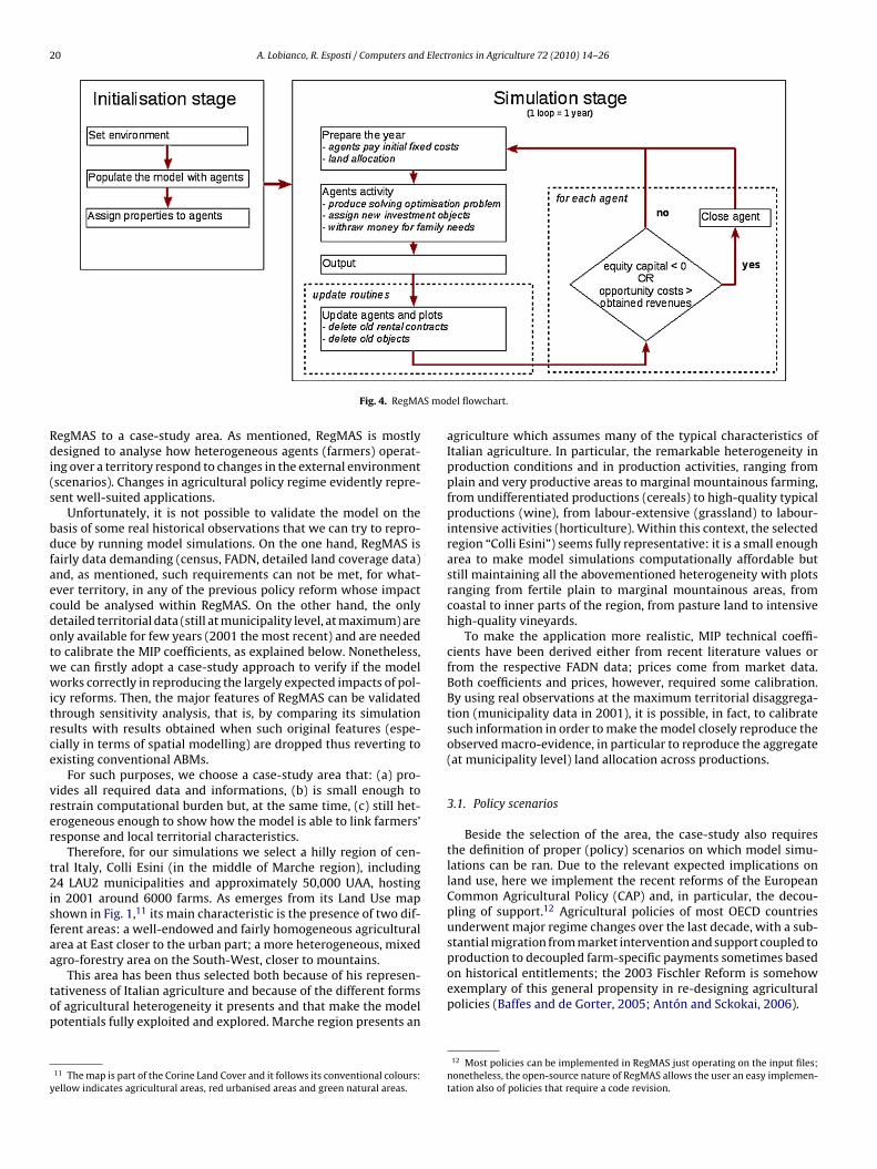
Fig. 4 summarizes the main logical steps of the model. As typi-al in ABMs, the initialisation stage is critical because the relevantharacteristics of the “real world” must be incorporated in theodel (see also Section 2.3.1), the agents must be entered and

hey must be endowed with the relevant objects, in our case pro-uction factors. After initialisation the model can proceed intohe simulation stage; simulation is organised in loops: any yearand is allocated to farmers; thereafter, they can activate pro-uction activities by solving their optimisation problem. Beforeroceeding to the next year, the model updates all the relevantexogenous) variables and select those farmers that can continuehe activity while others exit the business whenever their equityapital goes to zero or off-farm opportunity costs exceed farmrofit.

To run simulations, RegMAS solves a MIP problem like (6) forny individual farm and in several steps during each simulatederiod, resulting in thousand computations for each period, thoughhe “filtering” procedure illustrated above substantially reduces the

9 Analysing the Italian Corine Land Cover data between 1990 and 2000, Lobianco2006) highlights that the largest change in agricultural land use, beside the shift tother agricultural uses, concerns reallocation to urban uses, revealing a competitionetween these two land destinations.

es with main attributes and relations.

matrix activity size. It follows that the speed of the solving algo-rithm becomes a critical factor.

In fact, RegMAS uses external libraries to speed-up the solvingalgorithm. RegMAS class Opt is responsible to establish the direc-tion of the objective function (in our case, a maximisation), the set ofbounds, objective coefficients and constraint coefficients. Then, theproblem “object” is solved calling an external Dynamically LinkedLibrary (DLL). RegMAS uses the open-source GNU Linear Program-ming Kit (GLPK) (Makhorin, 2007) that firstly applies a two-stagerevised simplex method for continuous solutions and then a Branch& Bound method in case of integer optimisation.

From the computational point of view this latter methodology isparticularly helpful. In fact, MIP problems are more computation-ally demanding than LP (Linear Programming) problems. However,the Branch & Bound method, by partitioning the maximisationproblem in sub-problems whose upper and lower possible solu-tions are reciprocally compared, allows for an efficient search ofthe optimal solution over a much smaller domain.10

3. Model verification and validation: a case-study

application

To assess whether the depicted model works correctly and isable to properly and plausibly reproduce the real world, we apply

10 Sub-problems with an upper bound lower than any other sub-problem lowerbound are automatically eliminated from the search.

20 A. Lobianco, R. Esposti / Computers and Electronics in Agriculture 72 (2010) 14–26

S mod

Rdi(s

bdfaecdotwwitrce

vrer

t2isfaa

top

y

production to decoupled farm-specific payments sometimes based

Fig. 4. RegMA

egMAS to a case-study area. As mentioned, RegMAS is mostlyesigned to analyse how heterogeneous agents (farmers) operat-

ng over a territory respond to changes in the external environmentscenarios). Changes in agricultural policy regime evidently repre-ent well-suited applications.

Unfortunately, it is not possible to validate the model on theasis of some real historical observations that we can try to repro-uce by running model simulations. On the one hand, RegMAS isairly data demanding (census, FADN, detailed land coverage data)nd, as mentioned, such requirements can not be met, for what-ver territory, in any of the previous policy reform whose impactould be analysed within RegMAS. On the other hand, the onlyetailed territorial data (still at municipality level, at maximum) arenly available for few years (2001 the most recent) and are neededo calibrate the MIP coefficients, as explained below. Nonetheless,e can firstly adopt a case-study approach to verify if the modelorks correctly in reproducing the largely expected impacts of pol-

cy reforms. Then, the major features of RegMAS can be validatedhrough sensitivity analysis, that is, by comparing its simulationesults with results obtained when such original features (espe-ially in terms of spatial modelling) are dropped thus reverting toxisting conventional ABMs.

For such purposes, we choose a case-study area that: (a) pro-ides all required data and informations, (b) is small enough toestrain computational burden but, at the same time, (c) still het-rogeneous enough to show how the model is able to link farmers’esponse and local territorial characteristics.

Therefore, for our simulations we select a hilly region of cen-ral Italy, Colli Esini (in the middle of Marche region), including4 LAU2 municipalities and approximately 50,000 UAA, hosting

n 2001 around 6000 farms. As emerges from its Land Use maphown in Fig. 1,11 its main characteristic is the presence of two dif-erent areas: a well-endowed and fairly homogeneous agriculturalrea at East closer to the urban part; a more heterogeneous, mixedgro-forestry area on the South-West, closer to mountains.

This area has been thus selected both because of his represen-ativeness of Italian agriculture and because of the different formsf agricultural heterogeneity it presents and that make the modelotentials fully exploited and explored. Marche region presents an

11 The map is part of the Corine Land Cover and it follows its conventional colours:ellow indicates agricultural areas, red urbanised areas and green natural areas.

el flowchart.

agriculture which assumes many of the typical characteristics ofItalian agriculture. In particular, the remarkable heterogeneity inproduction conditions and in production activities, ranging fromplain and very productive areas to marginal mountainous farming,from undifferentiated productions (cereals) to high-quality typicalproductions (wine), from labour-extensive (grassland) to labour-intensive activities (horticulture). Within this context, the selectedregion “Colli Esini”) seems fully representative: it is a small enougharea to make model simulations computationally affordable butstill maintaining all the abovementioned heterogeneity with plotsranging from fertile plain to marginal mountainous areas, fromcoastal to inner parts of the region, from pasture land to intensivehigh-quality vineyards.

To make the application more realistic, MIP technical coeffi-cients have been derived either from recent literature values orfrom the respective FADN data; prices come from market data.Both coefficients and prices, however, required some calibration.By using real observations at the maximum territorial disaggrega-tion (municipality data in 2001), it is possible, in fact, to calibratesuch information in order to make the model closely reproduce theobserved macro-evidence, in particular to reproduce the aggregate(at municipality level) land allocation across productions.

3.1. Policy scenarios

Beside the selection of the area, the case-study also requiresthe definition of proper (policy) scenarios on which model simu-lations can be ran. Due to the relevant expected implications onland use, here we implement the recent reforms of the EuropeanCommon Agricultural Policy (CAP) and, in particular, the decou-pling of support.12 Agricultural policies of most OECD countriesunderwent major regime changes over the last decade, with a sub-stantial migration from market intervention and support coupled to

on historical entitlements; the 2003 Fischler Reform is somehowexemplary of this general propensity in re-designing agriculturalpolicies (Baffes and de Gorter, 2005; Antón and Sckokai, 2006).

12 Most policies can be implemented in RegMAS just operating on the input files;nonetheless, the open-source nature of RegMAS allows the user an easy implemen-tation also of policies that require a code revision.

A. Lobianco, R. Esposti / Computers and Electronics in Agriculture 72 (2010) 14–26 21

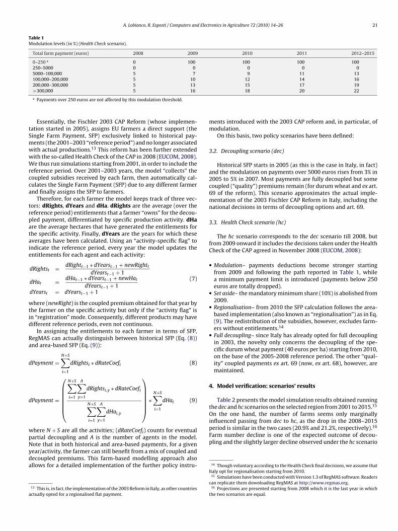
Table 1Modulation levels (in %) (Health Check scenario).

Total farm payment (euros) 2008 2009 2010 2011 2012–2015

0–250 a 0 100 100 100 100250–5000 0 0 0 0 05000–100,000 5 7 9 11 13100,000–200,000 5 10 12 14 16200,000–300,000 5 13 15 17 19

tSmwwWrcca

trpataie

wtid

Ra

d

d

wpNyda

a

On the one hand, the number of farms seems only marginallyinfluenced passing from dec to hc, as the drop in the 2008–2015period is similar in the two cases (20.9% and 21.2%, respectively).16

Farm number decline is one of the expected outcome of decou-

>300,000 5 16

a Payments over 250 euros are not affected by this modulation threshold.

Essentially, the Fischler 2003 CAP Reform (whose implemen-ation started in 2005), assigns EU farmers a direct support (theingle Farm Payment, SFP) exclusively linked to historical pay-ents (the 2001–2003 “reference period”) and no longer associatedith actual productions.13 This reform has been further extendedith the so-called Health Check of the CAP in 2008 (EUCOM, 2008).e thus run simulations starting from 2001, in order to include the

eference period. Over 2001–2003 years, the model “collects” theoupled subsidies received by each farm, then automatically cal-ulates the Single Farm Payment (SFP) due to any different farmernd finally assigns the SFP to farmers.

Therefore, for each farmer the model keeps track of three vec-ors: dRights, dYears and dHa. dRights are the average (over theeference period) entitlements that a farmer “owns” for the decou-led payment, differentiated by specific production activity. dHare the average hectares that have generated the entitlements forhe specific activity. Finally, dYears are the years for which theseverages have been calculated. Using an “activity-specific flag” tondicate the reference period, every year the model updates thentitlements for each agent and each activity:

dRightst = dRightt−1 ∗ dYearst−1 + newRightt

dYearst−1 + 1

dHat = dHat−1 ∗ dYearst−1 + newHat

dYearst−1 + 1dYearst = dYearst−1 + 1

(7)

here (newRight) is the coupled premium obtained for that year byhe farmer on the specific activity but only if the “activity flag” isn “registration” mode. Consequently, different products may haveifferent reference periods, even not continuous.

In assigning the entitlements to each farmer in terms of SFP,egMAS can actually distinguish between historical SFP (Eq. (8))nd area-based SFP (Eq. (9)):

Payment =N+S∑i=1

dRightsi ∗ dRateCoefi (8)

Payment =

⎛⎜⎜⎜⎜⎜⎝

N+S∑i=1

A∑y=1

dRightsi,y ∗ dRateCoefi

N+S∑i=1

A∑y=1

dHai,y

⎞⎟⎟⎟⎟⎟⎠

∗N+S∑i=1

dHai (9)

here N + S are all the activities; (dRateCoefi) counts for eventualartial decoupling and A is the number of agents in the model.

ote that in both historical and area-based payments, for a givenear/activity, the farmer can still benefit from a mix of coupled andecoupled premiums. This farm-based modelling approach alsollows for a detailed implementation of the further policy instru-

13 This is, in fact, the implementation of the 2003 Reform in Italy, as other countriesctually opted for a regionalised flat payment.

18 20 22

ments introduced with the 2003 CAP reform and, in particular, ofmodulation.

On this basis, two policy scenarios have been defined:

3.2. Decoupling scenario (dec)

Historical SFP starts in 2005 (as this is the case in Italy, in fact)and the modulation on payments over 5000 euros rises from 3% in2005 to 5% in 2007. Most payments are fully decoupled but somecoupled (“quality”) premiums remain (for durum wheat and ex art.69 of the reform). This scenario approximates the actual imple-mentation of the 2003 Fischler CAP Reform in Italy, including thenational decisions in terms of decoupling options and art. 69.

3.3. Health Check scenario (hc)

The hc scenario corresponds to the dec scenario till 2008, butfrom 2009 onward it includes the decisions taken under the HealthCheck of the CAP agreed in November 2008 (EUCOM, 2008):

• Modulation– payments deductions become stronger startingfrom 2009 and following the path reported in Table 1, whilea minimum payment limit is introduced (payments below 250euros are totally dropped).

• Set aside– the mandatory minimum share (10%) is abolished from2009.

• Regionalisation– from 2010 the SFP calculation follows the area-based implementation (also known as “regionalisation”) as in Eq.(9). The redistribution of the subsidies, however, excludes farm-ers without entitlements.14

• Full decoupling– since Italy has already opted for full decouplingin 2003, the novelty only concerns the decoupling of the spe-cific durum wheat payment (40 euros per ha) starting from 2010,on the base of the 2005-2008 reference period. The other “qual-ity” coupled payments ex art. 69 (now, ex art. 68), however, aremaintained.

4. Model verification: scenarios’ results

Table 2 presents the model simulation results obtained runningthe dec and hc scenarios on the selected region from 2001 to 2015.15

pling and the slightly larger decline observed under the hc scenario

14 Though voluntary according to the Health Check final decisions, we assume thatItaly opt for regionalisation starting from 2010.

15 Simulations have been conducted with Version 1.3 of RegMAS software. Readerscan replicate them downloading RegMAS at http://www.regmas.org.

16 Projections are presented starting from 2008 which it is the last year in whichthe two scenarios are equal.

22 A. Lobianco, R. Esposti / Computers and Electronics in Agriculture 72 (2010) 14–26

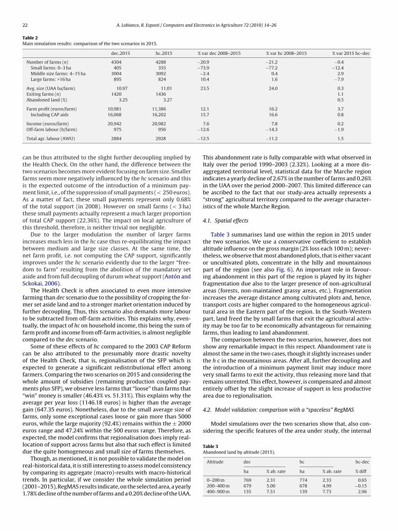
Table 2Main simulation results: comparison of the two scenarios in 2015.

dec 2015 hc 2015 % var dec 2008–2015 % var hc 2008–2015 % var 2015 hc–dec

Number of farms (n) 4304 4288 −20.9 −21.2 −0.4Small farms: 0–3 ha 405 355 −73.9 −77.2 −12.4Middle size farms: 4–15 ha 3004 3092 −2.4 0.4 2.9Large farms: >16 ha 895 824 10.4 1.6 −7.9

Avg. size (UAA ha/farm) 10.97 11.01 23.5 24.0 0.3Exiting farms (n) 1420 1436 1.1Abandoned land (%) 3.25 3.27 0.5

Farm profit (euros/farm) 10,981 11,386 12.1 16.2 3.7Including CAP aids 16,068 16,202 15.7 16.6 0.8

−1

−1

cttfimAotot

ibnidaS

fmfttfc

coefwm“agfeeeld

rbt(1

4.2. Model validation: comparison with a “spaceless” RegMAS

Model simulations over the two scenarios show that, also con-sidering the specific features of the area under study, the internal

Table 3Abandoned land by altitude (2015).

Altitude dec hc hc-dec

Income (euros/farm) 20,942 20,982Off-farm labour (h/farm) 975 956

Total agr. labour (AWU) 2884 2928

an be thus attributed to the slight further decoupling implied byhe Health Check. On the other hand, the difference between thewo scenarios becomes more evident focusing on farm size. Smallerarms seem more negatively influenced by the hc scenario and thiss the expected outcome of the introduction of a minimum pay-

ent limit, i.e., of the suppression of small payments (< 250 euros).s a matter of fact, these small payments represent only 0.68%f the total support (in 2008). However on small farms (< 3 ha)hese small payments actually represent a much larger proportionf total CAP support (22.36%). The impact on local agriculture ofhis threshold, therefore, is neither trivial nor negligible.

Due to the larger modulation the number of larger farmsncreases much less in the hc case thus re-equilibrating the impactetween medium and large size classes. At the same time, theet farm profit, i.e. not computing the CAP support, significantly

mproves under the hc scenario evidently due to the larger “free-om to farm” resulting from the abolition of the mandatory setside and from full decoupling of durum wheat support (Antón andckokai, 2006).

The Health Check is often associated to even more intensivearming than dec scenario due to the possibility of cropping the for-

er set aside land and to a stronger market orientation induced byurther decoupling. Thus, this scenario also demands more labouro be subtracted from off-farm activities. This explains why, even-ually, the impact of hc on household income, this being the sum ofarm profit and income from off-farm activities, is almost negligibleompared to the dec scenario.

Some of these effects of hc compared to the 2003 CAP Reforman be also attributed to the presumably more drastic noveltyf the Health Check, that is, regionalisation of the SFP which isxpected to generate a significant redistributional effect amongarmers. Comparing the two scenarios on 2015 and considering thehole amount of subsidies (remaining production coupled pay-ents plus SFP), we observe less farms that “loose” than farms that

win” money is smaller (46.43% vs. 51.31%). This explains why theverage per year loss (1146.18 euros) is higher than the averageain (647.35 euros). Nonetheless, due to the small average size ofarms, only some exceptional cases loose or gain more than 5000uros, while the large majority (92.4%) remains within the ± 2000uros range and 47.24% within the 500 euros range. Therefore, asxpected, the model confirms that regionalisation does imply real-ocation of support across farms but also that such effect is limitedue the quite homogeneous and small size of farms themselves.

Though, as mentioned, it is not possible to validate the model on

eal-historical data, it is still interesting to assess model consistencyy comparing its aggregate (macro)-results with macro-historicalrends. In particular, if we consider the whole simulation period2001–2015), RegMAS results indicate, on the selected area, a yearly.78% decline of the number of farms and a 0.20% decline of the UAA.

7.6 7.8 0.22.6 −14.3 −1.9

2.5 −11.2 1.5

This abandonment rate is fully comparable with what observed inItaly over the period 1990–2003 (2.32%). Looking at a more dis-aggregated territorial level, statistical data for the Marche regionindicates a yearly decline of 2.67% in the number of farms and 0.26%in the UAA over the period 2000–2007. This limited difference canbe ascribed to the fact that our study-area actually represents a“strong” agricultural territory compared to the average character-istics of the whole Marche Region.

4.1. Spatial effects

Table 3 summarises land use within the region in 2015 underthe two scenarios. We use a conservative coefficient to establishaltitude influence on the gross margin (2% loss each 100 m); never-theless, we observe that most abandoned plots, that is either vacantor uncultivated plots, concentrate in the hilly and mountainouspart of the region (see also Fig. 6). An important role in favour-ing abandonment in this part of the region is played by its higherfragmentation due also to the larger presence of non-agriculturalareas (forests, non-maintained grassy areas, etc.). Fragmentationincreases the average distance among cultivated plots and, hence,transport costs are higher compared to the homogeneous agricul-tural area in the Eastern part of the region. In the South-Westernpart, land freed the by small farms that exit the agricultural activ-ity may be too far to be economically advantageous for remainingfarms, thus leading to land abandonment.

The comparison between the two scenarios, however, does notshow any remarkable impact in this respect. Abandonment rate isalmost the same in the two cases, though it slightly increases underthe h c in the mountainous areas. After all, further decoupling andthe introduction of a minimum payment limit may induce morevery small farms to exit the activity, thus releasing more land thatremains unrented. This effect, however, is compensated and almostentirely offset by the slight increase of support in less productivearea due to regionalisation.

ha % ab. rate ha % ab. rate % diff

0–200 m 769 2.31 774 2.33 0.65200–400 m 679 5.00 678 4.99 −0.15400–900 m 135 7.51 139 7.73 2.96

A. Lobianco, R. Esposti / Computers and Electronics in Agriculture 72 (2010) 14–26 23

Table 4Sensitivity analysis on transport costs and gross margin reduction with altitude (%difference with respect to the hc scenario in 2015).

noTC 2× TC 10× TC noAltC 2× AltC 10× AltC

N farms −6.3 + 1.9 −6.9 + 2.7 −1.5 −16.2Total income + 0.7 −2.3 −34.7 + 2.1 −1.0 −21.0

Rental pricesArable dry + 22.7 −20.1 −90.5 + 4.6 −7.0 −47.9Arable irrigable + 7.9 −1.2 −25.6 + 18.9 −11.2 −82.9Wine + 3.2 −3.4 −19.4 + 11.1 −13.2 −71.1Fruit −1.1 −7.7 −17.9 + 9.0 −11.6 −65.0Olive + 5.6 + 6.1 −10.9 + 6.3 −7.3 −66.5Pasture + 110.6 −49.7 −98.8 + 16.5 + 1.3 −76.2

Abandoned land + 15.3 + 1.4 + 892.4 −8.3 + 3.2 + 134.7

noTC, 2× TC, 10× TC indicate no transport costs, double and 10 times transport costswngr

semtcmtictwd

lwsotfiagdaipcaafbtntkcfvt

eTte

r

Table 5The impact of AltC on abandonment rate in 2015 (%).

Altitude Land abandonment rate

hc scenario noAltC 2× AltC 10× AltC

spatial features are actually attributed to plots on a random basisrather than on the basis of the real land use coverage. Nonetheless,this latter solution would not be able to associate to this macro-evidence the correct impact on land use (the micro-level). To showthis specific feature of RegMAS, a second sensitivity analysis con-

ith respect to the hc scenario, respectively.oAltC, 2× AltC, 3× AltC indicate no variation, double and 10 times variation ofross margin with altitude compared to the original scenario (2% loss any 100 m),espectively.

tructure of RegMAS seems consistent with the real world as it gen-rates those effects that are generally expected, in direction andagnitude, from the introduction of the hc measures. Nonetheless,

hese aggregate results could be obtained by a properly definedonventional ABM, as well. To validate the original features of theodel, that is, in particular, to demonstrate the advantages of spa-

ial explicit modelling, we need to assess which kind of additionalnformation such features (i.e., spatial explicitness) can provideompared to conventional ABMs. To pursue this kind of valida-ion we carry out sensitivity analysis by comparing RegMAS resultsith those obtained by a RegMAS model where spatial features areropped.

Firstly, we run the model without spatial influence on costs andand renting, that is, no transport Costs (TC) and, at the opposite,

ith TC augmented two and ten times, respectively. Moreover,pace influences performance and renting behaviour also in termsf altitude. As mentioned, in RegMAS a simple coefficient simulateshe reduction of gross margin due to altitude (the altitudinal coef-cient, AltC). Therefore, we also perform model simulations underlternative values of the gross margin reduction coefficient: theross margin declines with the altitude at 0%, 4% (double than stan-ard 2%) and 20% (ten times), respectively. Results of this sensitivitynalysis are reported in Table 4.17 When the spatial dimension (thats, distance and TC) is skipped, farms loose their advantage on closelots and enter a greater competition for land renting. Such moreompetitive environment leads to a reduction of the number ofctive farms. The opposite happens when transport costs increasend, thus, space acts as a non-competitive factor: the number ofarms increases. This latter effect disappears, however, when TCecome too high: they negatively affect farmer profit in such a wayhat a larger land abandonment occurs. Therefore, TC have a directegative influence on farm profit and income but, at the same time,his effect may be counterbalanced by the impact on land mar-et. With lower TC farms save costs but have to face the higherompetition for land, resulting in higher rental prices, especiallyor activities with lower gross margin and on which, evidently, TCariations have a larger impact in terms of economic convenienceo continue production (i.e., pasture land).

RegMAS thus seems fully capable of representing this not trivial

ffect of space (through TC) on farm performance and behaviour.his capability is also confirmed by results obtained under alterna-ive responses of gross margin to altitude. As the AltC coefficient isxpressed as a proportion of gross margin, productions with higher

17 Analogous results can be obtained under scenario dec; results are available onequest.

0–200 m 2.33 2.18 2.43 3.33200–400 m 4.99 4.38 5.06 15.19400–900 m 7.73 7.17 7.78 30.31

gross margins (e.g., wine and fruits & vegetable) are expected to be,in absolute terms, more sensitive to AltC while for TC the oppositeholds true. This expectation is confirmed by results if we comparethe impact of AltC variation on arable crops cultivated on dry landand on irrigable land (where gross margin is expected to be higher).

Another difference with TC is that AltC affects farm perfor-mance in a univocal way: if AltC decreases, performance improvesin hilly and mountainous farming; the opposite occurs when AltCincreases. This affects the number of active farms and, as a con-sequence, land abandonment. Table 5 reports the abandonmentrates under the alternative AltC values compared to the baselinehc scenario. Results show that the response of abandonment toAltC variations is relatively inelastic. While abandonment remainsalmost unaffected in plain areas regardless AltC, as obvious, a largeimpact in hilly and mountainous areas can be observed only whenthe reduction of gross margin with altitude becomes very intense(20% loss any 100 meters).

It may be argued that the capacity of RegMAS to take intoaccount space (as distance/TC and altitude) in generating aggregate(macro)-results can be also obtained in conventional ABMs where

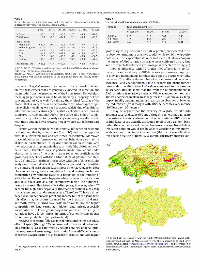
Fig. 5. Land use classes and DTM in the real RegMAS simulation area (a) and in therandomly shuffled case (b). Map colours refer to the standard Corine Land Coverlegend, downloadable from http://dataservice.eea.europa.eu. (For interpretation ofthe references to colour in this figure legend, the reader is referred to the web versionof the article.)

24 A. Lobianco, R. Esposti / Computers and Electronics in Agriculture 72 (2010) 14–26

Table 6Results robustness: results of five simulation repetitions with different random number seed, hc scenario in 2015).

Full region (48,679 ha UAA) Sub-region (931 ha UAA)

avg. st. err. cv avg. st. err. cv

Number of farms (n) 4294 11.9 0.0028 87 2.8 0.0320Avg. size (UAA ha/farm) 10.98 0.0 0.0027 10.7 0.4 0.0410Exiting farms (n) 1430 11.9 0.0083 23 2.8 0.1196Abandoned land (%) 3.31 0.0 0.0139 0.8 0.2 0.2187Farm profit (euros/farm) 11,340 55.3 0.0049 12,834 353.1 0.0275

Including CAP aids (euros/farm) 16,148 53.5 0.0033 17,394 274.7 0.0158

sittmtataucangor

iirm(

Fsit

Income (euros/farm) 20,929 48.3Off-farm labour (h/farm) 956 9.4

Total agr. labour (AWU) 2928 26.4

ists in running the model on the same region but with all spatialnformation (land coverage and DTM, Digital Terrain Model, for alti-ude) randomly shuffled (rand space). Fig. 5 graphically compareshe two cases: Fig. 5(a) shows land coverage and altimetric infor-

ation as they enter RegMAS simulations with plots associated tohe real land use; Fig. 5(b) shows how the area looks like when plotsre assigned randomly. As evident, when the “real” spatial informa-ion is dropped, we miss the link between real local conditions andgents’ behaviours. In particular, randomizing the space, we arenable to take into account those special and somehow extremeonditions of marginality that may induce farms to exit the activitynd, therefore, to release or abandon land. Consequently, it shouldot surprise that the rand space case also reports different aggre-ate (macro)-results: a higher number of active farming at the endf the simulation (+3.73% in 2015) and a lower land abandonmentate (−12.4%).

Moreover, while in RegMAS results indicate a strong differencen land abandonment rate between plain and mountainous areas,

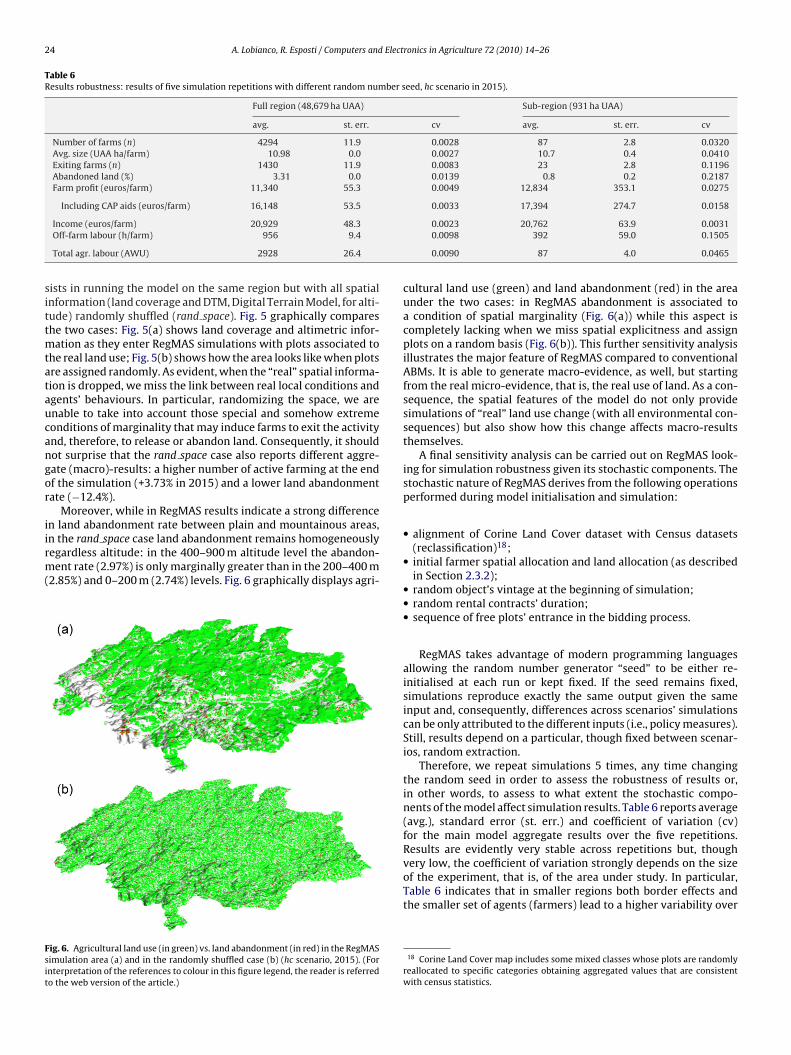
n the rand space case land abandonment remains homogeneouslyegardless altitude: in the 400–900 m altitude level the abandon-ent rate (2.97%) is only marginally greater than in the 200–400 m

2.85%) and 0–200 m (2.74%) levels. Fig. 6 graphically displays agri-

ig. 6. Agricultural land use (in green) vs. land abandonment (in red) in the RegMASimulation area (a) and in the randomly shuffled case (b) (hc scenario, 2015). (Fornterpretation of the references to colour in this figure legend, the reader is referredo the web version of the article.)

0.0023 20,762 63.9 0.00310.0098 392 59.0 0.1505

0.0090 87 4.0 0.0465

cultural land use (green) and land abandonment (red) in the areaunder the two cases: in RegMAS abandonment is associated toa condition of spatial marginality (Fig. 6(a)) while this aspect iscompletely lacking when we miss spatial explicitness and assignplots on a random basis (Fig. 6(b)). This further sensitivity analysisillustrates the major feature of RegMAS compared to conventionalABMs. It is able to generate macro-evidence, as well, but startingfrom the real micro-evidence, that is, the real use of land. As a con-sequence, the spatial features of the model do not only providesimulations of “real” land use change (with all environmental con-sequences) but also show how this change affects macro-resultsthemselves.

A final sensitivity analysis can be carried out on RegMAS look-ing for simulation robustness given its stochastic components. Thestochastic nature of RegMAS derives from the following operationsperformed during model initialisation and simulation:

• alignment of Corine Land Cover dataset with Census datasets(reclassification)18;

• initial farmer spatial allocation and land allocation (as describedin Section 2.3.2);

• random object’s vintage at the beginning of simulation;• random rental contracts’ duration;• sequence of free plots’ entrance in the bidding process.

RegMAS takes advantage of modern programming languagesallowing the random number generator “seed” to be either re-initialised at each run or kept fixed. If the seed remains fixed,simulations reproduce exactly the same output given the sameinput and, consequently, differences across scenarios’ simulationscan be only attributed to the different inputs (i.e., policy measures).Still, results depend on a particular, though fixed between scenar-ios, random extraction.

Therefore, we repeat simulations 5 times, any time changingthe random seed in order to assess the robustness of results or,in other words, to assess to what extent the stochastic compo-nents of the model affect simulation results. Table 6 reports average(avg.), standard error (st. err.) and coefficient of variation (cv)for the main model aggregate results over the five repetitions.

Results are evidently very stable across repetitions but, thoughvery low, the coefficient of variation strongly depends on the sizeof the experiment, that is, of the area under study. In particular,Table 6 indicates that in smaller regions both border effects andthe smaller set of agents (farmers) lead to a higher variability over

18 Corine Land Cover map includes some mixed classes whose plots are randomlyreallocated to specific categories obtaining aggregated values that are consistentwith census statistics.

d Elect

tmmabi(tiabff

5

td(trstrm

rRambepmmma

n(itkna

flsmmttiaaf

tpc

n

A. Lobianco, R. Esposti / Computers an

he stochastic components.19 This evidence represents an argu-ent in favour of applying RegMAS to larger regions as this impliesore robust results in simulation analysis. Larger regions, however,

lso brings about a higher computational burden. This trade-offetween robustness and computational costs is actually minimised

n RegMAS compared to other simulation toolkits. Castella et al.2005), for instance, use the Cormas Toolkit (Bousquet et al., 1998)o perform simulations on a relatively small (50 × 50) grid,20 thusmplying much lower computational burden but lower robustness,s well. Nonetheless, even in RegMAS the optimal compromiseetween these two aspects, and, therefore, the optimal regional sizeor application, is still to be found and deserves further attention inuture research.

. Concluding remarks

This paper presents and tests RegMAS, an open-source, spa-ially explicit agent based modelling framework (and software),esigned to assess the possible impact of alternative scenariosmainly changes in policy regime) on heterogeneous farm struc-ures, income and land use. The main original feature of RegMASests on the fact that it allows agents (farmers) to take into accountpatially explicit information in formulating their behaviours and,hus, it allows assessing the consequent economic (as well as envi-onmental) outcome at both the micro (plot-by-plot)- and theacro (aggregate)-levels.By assessing its functioning on a portion of a central Italian

egion (Marche) and under two alternative CAP scenarios (the 2003eform and the Health Check), our simulation demonstrates thedvantages of such spatial explicitness. Results suggest that theodel behaves as expected in all major aspects and, thus, it can

e used to derive the aggregate response of a complex and het-rogeneous system whenever the external environment (and, inarticular, the policy regime) is exogenously modified. Further-ore, by making the spatial dimension explicit, RegMAS seemsore able, compared to conventional ABMs, to associate theseacro-results to the underlying micro (land use)-behaviours such

s lent renting, land abandonment, and exiting the business.As the major purpose of the paper is to provide an origi-

al contribution on explicit spatial modelling within conventionalspaceless) ABMs, simulation results specifically emphasize thenteresting insights concerning the often disregarded effects ofransport costs and loss of margins due to altitude which allow suchind of models to generate more plausible results on how exter-al changes (policy reform, in the present case) impact agriculturalctivity.

Though here applied to specific policy measures, RegMAS isexible enough to allow adaptation over a large set of differentcenarios (change in agricultural prices, introduction of environ-ental regulations, introduction of new technologies, etc.). Thisore extensive application can be one possible direction of fur-

her research on this modelling tool. Further effort is also neededo assess the optimal geographical size of model application and

n improving its original features especially concerning how spaceffects land market, transport costs, performance and agents’ inter-ction. Eventually, as on open-source software, RegMAS can beurther developed in these or other directions by user themselves.

19 Here “border effects” indicate the effects on agent’s behaviour of being close tohe borders of the simulation area. Spatial simulations can avoid border effects usingeriodic boundary conditions (e.g. running the simulation on a toroidal surface) oran reduce them using a larger region.20 In comparison, the present simulations are ran on a 396 × 301 grid, with 69,143on-zero cells.

ronics in Agriculture 72 (2010) 14–26 25

Acknowledgements

Authorship may be attributed as follows: Sections 2 and 4 toLobianco, Sections 1, 3 and 5 to Esposti. A. Lobianco wish to thankthe IAMO team for their support and training on agent-based mod-elling. The authors also thank two anonymous referees and theEditor for their helpful suggestions and remarks on a previous ver-sion of the paper.

Appendix A. Supplementary data

Supplementary data associated with this article can be found, inthe online version, at doi:10.1016/j.compag.2010.02.006.

References

Antón, J., Sckokai, P., 2006. The challenge of decoupling agricultural support. Euro-Choices 5 (3), 13–19.

Arfini, F., 2000. I modelli di programmazione matematica per l’analisi della politicaagricola comune. In: INEA seminar Valutare gli effetti della Politica Agri-cola Comune, Rome, 24 October 2000. Available from: http://web.archive.org/web/20041024164241/http://www.inea.it/opaue/pac/arfini.PDF.

Baffes, J., de Gorter, H., 2005. Experience with decoupling agricultural support. In:Aksoy, M.A., Beghin, J.C. (Eds.), Global Agricultural Trade and Developing Coun-tries. World Bank Publications, pp. 75–89.

Balmann, A., 1997. Farm-based modelling of regional structural change: A cellu-lar automata approach. European Review of Agricultural Economics 24 (1–2),85–108, doi:10.1093/erae/24.1-2.85.

Boero, R., 2006. The spatial dimension and social simulations: a review of threebooks, JASSS. Journal of Artificial Societies and Social Simulation, Available from:http://jasss.soc.surrey.ac.uk/9/4/reviews/boero.html.

Bousquet, F., Bakam, I., Proton, H., Page, C.L., 1998. CORMAS: common-pool resourcesand multi-agent systems. In: del Pobil, A.P., Mira, J., Ali, M. (Eds.), Tasks and Meth-ods in Applied Artificial Intelligence, vol. 1416 of Lecture Notes in ComputerScience. Springer, pp. 826–837.

Brady, M., Kellermann, K., Sahrbacher, C., Jelinek, L., 2009. Impacts of decou-pled agricultural support on landscape values: an EU-wide assessment.Journal of Agricultural Economics 60 (3), 563–585, doi:10.1111/j.1477-9552.2009.00216.x.

Castella, J., Boissau, S., Trung, T., Quang, D., 2005. Agrarian transition andlowland-upland interactions in mountain areas in northern Vietnam:application of multi-agent simulation model. Agricultural Systems. Avail-able from: http://www.sciencedirect.com/science/article/B6T3W-4F29HSM-1/2/5d018e2f9b940709e3857c26d8d1f86d.

Ellis, J.R., Hughes, D.W., Butcher, W.R., 1991. Economic modeling of farm productionand conservation decisions in response to alternative resource and environmen-tal policies. Northeastern Journal of Agricultural and Resource Economics 20 (1),98–108, Available from: http://econpapers.repec.org/RePEc:ags:nejare:28822.

EUCOM, 2008. Proposal for a council regulation establishing common rulesfor direct support schemes for farmers under the common agriculturalpolicy and establishing certain support schemes for farmers. COM 306.Commission of the European Communities, 20 May 2008. Available from:http://ec.europa.eu/agriculture/healthcheck/prop en.pdf.

Happe, K., Balmann, A., Kellermann, K., Sahrbacher, C., 2008. Does structurematter? the impact of switching the agricultural policy regime on farmstructures. Journal of Economic Behavior & Organization 67 (2), 431–444,doi:10.1016/j.jebo.2006.10.009.

Happe, K., Kellermann, K., Balmann, A., 2006. Agent-based analysis of agricul-tural policies: an illustration of the agricultural policy simulator agripolis,its adaptation, and behavior. Ecology and Society 11 (1), 49, Available from:http://www.ecologyandsociety.org/vol11/iss1/art49/ES-2006–1741.pdf.

Hazell, P.B., Norton, R.D., 1986. Mathematical Programming for Economic Analysisin Agriculture. Macmillan, New York.

Heckelei, T., Britz, W., 2005. Models based on positive mathematical programming:state of the art and further extensions. In: Arfini, F. (Ed.), Modelling AgriculturalPolicies: State of the Art and New Challenges. Proceedings of the 89th Euro-pean Seminar of the European Association of Agricultural Economics. MonteUniversitá Parma, pp. 48–73.

Kellermann, K., Happe, K., Sahrbacher, C., Brady, M., 2007. Agripolis2.0—documentation of the extended model. IDEMA Working Paper 20.Available from: http://www.sli.lu.se/IDEMA/WPs/IDEMA deliverable 20.pdf.

Kellermann, K., Sahrbacher, C., Balmann, A., 2008. Land markets in agentbased models of structural change. In: Modelling Agricultural and RuralDevelopment Policies. 107th EAAE Seminar, Sevilla. Available from:

http://agecon.lib.umn.edu/cgi-bin/pdf view.pl?paperid=29447&ftype=.pdf.

Lobianco, A., 2006. Il sistema agricolo ed alimentare nelle Marche. Rapporto 2005.Edizioni Scientifiche Italiane, pp. 71–81 (Chapter 2.1).

Lobianco, A., 2007. The effects of decoupling on two Italian regions. an agent-based model. Associazione Bartola Ph.D. Studies, p. 2. Available from: http://associazionebartola.univpm.it/pubblicazioni/phdstudies/phdstudies2.pdf.

2 Elect

M

P

P

P

Romero, C., Rehman, T., 2003. Multiple criteria analysis for agricultural decisions.In: Developments in Agricultural Economics, 2nd ed. Elsevier.

6 A. Lobianco, R. Esposti / Computers and

akhorin, A., 2007. Gnu Linear Programming Kit. Reference Manual. Available from:http://www.gnu.org/software/glpk/.

aris, Q., 1991. An Economic Interpretation of Linear Programming. Iowa StateUniversity Press. Also Available in Italian with Title Programmazione lineare.

Un’interpretazione economica.

arker, D.C., 2003. Multi-agent systems for the simulation of land-use and land-cover change: A review. Annals of the Association of American Geographers 93(2), 314–337, doi:10.1111/1467-8306.9302004.

iorr, A., Ungaro, F., Ciancaglini, A., Happe, K., Sahrbacher, A., Sattler, C., Uthes,S., Zander, P., 2009. Integrated assessment of future cap policies: land use

ronics in Agriculture 72 (2010) 14–26

changes, spatial patterns and targeting. Environmental Science and Policy, 12(8), 1122–1136.

Sahrbacher, C., Schnicke, H., Happe, K., Graubner, M., 2005. Adapta-tion of agent-based model agripolis to 11 study regions in theenlarged European union. IDEMA Working Paper 10. Available from:http://www.sli.lu.se/IDEMA/WPs/IDEMA deliverable 10.pdf.